21 Orthogonal Polynomials We can construct a polynomial orthonormal basis of a Hilbert space. They are called orthogonal polynomials, which have a beautiful general theory and many important numerical applications ( ---t 22). Key words: generalized Fourier expansion, generalized Ro- drigues' formula, generating function, three term recursion relation, zeros, Sturm's theorem, Legendre polynomial, Her- mite polynomial, Chebychev polynomial Summary: (1) Recognize that there is a set of relations and formulas common to many (all classical) orthogonal polynomials (21A.3-11). (2) Generating function is a useful tool to derive recursion relations (21B.4, for example). (3) Remember where the representative polynomials - Legendre, Her- mite, and Chebychev - appear (21B). 21.A General Theory 21A.l Existence of general theory. The most important fact about orthonormal polynomials is that there is a general theory shared by all the families of (classical ---t21A.6 Discussion (A) ) orthogonal polyno- mials. The general theory includes generalized Rodrigues' formula, as- sociating (Sturm-Liouville type) eigenvalue problems, generating func- tions, three term recursion formulas, etc. 21A.2 Orthogonal polynomials for L 2 ([a, b]' w) via Gram-Schmidt. {l, x, x 2 , .•• } makes a complete set offunctions for L 2 ([a, b]' w) (---t20.19): notice first that CO([a, b]) (the totality of continuous functions on [a, b]) is dense in this space. Weierstrass' theorem (---t17.3) tells us that any continuous function on a finite interval can be uniformly approxi- mated by a polynomial. Hence, the totality of polynomials is dense in L 2 ((a, b), w). Therefore, the set of kets {In)} such that (xln) = x n308 is 308Por the notational convention see 20.21. 303

Welcome message from author
This document is posted to help you gain knowledge. Please leave a comment to let me know what you think about it! Share it to your friends and learn new things together.
Transcript
21 Orthogonal Polynomials
We can construct a polynomial orthonormal basis of a Hilbertspace. They are called orthogonal polynomials, which havea beautiful general theory and many important numericalapplications (---t 22).
Key words: generalized Fourier expansion, generalized Rodrigues' formula, generating function, three term recursionrelation, zeros, Sturm's theorem, Legendre polynomial, Hermite polynomial, Chebychev polynomial
Summary:(1) Recognize that there is a set of relations and formulas common tomany (all classical) orthogonal polynomials (21A.3-11).(2) Generating function is a useful tool to derive recursion relations(21B.4, for example).(3) Remember where the representative polynomials - Legendre, Hermite, and Chebychev - appear (21B).
21.A General Theory
21A.l Existence of general theory. The most important fact aboutorthonormal polynomials is that there is a general theory shared by allthe families of (classical ---t21A.6 Discussion (A) ) orthogonal polynomials. The general theory includes generalized Rodrigues' formula, associating (Sturm-Liouville type) eigenvalue problems, generating functions, three term recursion formulas, etc.
21A.2 Orthogonal polynomials for L2([a, b]' w) via Gram-Schmidt.{l, x, x2, .•• } makes a complete set offunctions for L2([a, b]' w) (---t20.19):notice first that CO([a, b]) (the totality of continuous functions on [a, b])is dense in this space. Weierstrass' theorem (---t17.3) tells us thatany continuous function on a finite interval can be uniformly approximated by a polynomial. Hence, the totality of polynomials is dense inL2((a, b), w). Therefore, the set of kets {In)} such that (xln) = xn308 is
308Por the notational convention see 20.21.
303
a complete set (-+20.3) of the Hilbert space L2([a, b], w). In this spacethe scalar product (-+20.5) is defined by
(fIg) _lb
f(x)g(x)w(x)dx, (21.1)
and the norm Ilfllw = JUII). We apply the Gram-Schmidt orthonormalization (-+20.16) to {In)} as follows:
(1) We define Ipo) = 10)//(010).(2) Normalizing 11) -IPo)(Poll), we construct Ipl)'(3) More generally, normalizing
n-l
In) - L IPk)(Pkl n ),k=O
(21.2)
we obtain IPn).{IPn)} is an orthonormal basis of L2([a, b], w).
The family of orthogonal polynomials of L2([a, b], w) is defined by(xIPn) times appropriate n-dependent numerical multiplicative factoras seen in 21A.5.
Exercise.Apply the Gram-Schmidt orthonormalization method to {xn}~=o and make an ONbasis for L2 ([O, 1]). Compute the basis up to the third member of the set.
21A.3 Theorem.(1) Pn(x) = (xIPn) is orthogonal to any (n - I)-order polynomial.(2) The orthonormal polynomials for L2 ([a, b], w) are unique, if the coefficients of the highest order terms are chosen to be positive.309
These assertions are obviously true by construction, but practically important.
21AA Least square approximation and generalized Fourier expansion. Let Pn be the totality of the polynomials order less than orequal to n. The polynomial P E Pn which minimizes
Ilf - Pllw (21.3)
for f E L2([a, b), w) is called the n-th order least square approximationof f (-+20.13). The ket IP) satisfying this condition is given by
n
IP) =L Ipj)(pjlj),j=O
(21.4)
309Here, it is not meant that the orthonormal basis in terms of polynomials isunique (of course, not). If we demand that there are no two polynomials of thesame order in the basis, the choice is unique.
304
(21.6)
where IPi) are calculated in 21A.2 with respect to w. That is, IP)is the n- th partial sum of the following generalized Fourier expansion(~20.14) of If)
00
If) = L Ipj)(pjlf)· (21.5)j=O
Notice that all the general properties of the Fourier series 17.5 applyhere as well.
Exercise.(1) Consider the step function (xla) = 0(x - a) on [-1,1] (a E (-1,1». Expandthis in terms of Legendre polynomials (-->21A.5).
(Pnl a) =V2(2n\ 1) (Pn-1(a) - Pn+1(a».
(pO Ia) = (1 - a) / y'2 as easily seen. Hence,
1 1 ex:>
0(x - a) = 2(1 - a) + 2 I)Pn-1(a) - Pn+1(a)]Pn(x). (21.7)n=!
(2) Expand x 5 into the generalized Fourier series in terms of Legendre polynomials.
21A.5 Example: Legendre polynomials. A family of orthogonalpolynomials of £2 ([-1, 1]) called the Legendre polynomials is definedas
Pn(x) = f2(xIPn) (21.8)y~
in terms of orthonormal kets {IPn)} constructed for a = -1, b = 1
and w = 1 in 21A.2. The coefficient J2/(2n + 1) is the multiplicativefactor mentioned in 21A.2. Pn(x) is called the n-th order Legendrepolynomial. According to our notational rule (~20.22)
11 V2n + 1(Pnlf) = -1 dx 2 Pn(x)f(x). (21.9)
Hence, the corresponding generalized Fourier expansion (21.5) in termsof the Legendre polynomials reads
00 2n + 1 [11 ]f(x) =~ 2 Pn(x) -1 dxPn(x)f(x) . (21.10)
21A.6 Generalized Rodrigues' formula. Let Fn(x) be defined on(a, b) eRas
(21.11)
305
(21.12)
where wand s are chosen as
a b w(x) s(x)a b (b - x)Q(x - a)f1 a.f3 > -1 (b-x)(x-a)a +00 e-X(x - a)f3 f3 > -1 x-a-00 +00 e- x2 1
As can easily be seen Fn is an n-th order polynomial (-t2A.l Exercise (D) )'1Fn(x)} is a orthogonal polynomial system for £2((a, b), w)(-t20.17),31 because
lb
dxw(x)Fn(x)Fm(x) = 0 for n =J m.(I
(Demonstrate this.) If the interval (a, b) and the weight function ware given, the orthogonal polynomial set311 is uniquely fixed as seenfrom the Gram-Schmidt construction (up to multiplicative constants)(-t21A.2).
For example, with w = 1 (that is, a = f3 = 0), a = -1 and b = 1,Fn must (-t21A.3) be proportional to the Legendre polynomial PnIndeed, from (21.11)
(21.13)
(21.14)
This is called Rodrigues' formula.With a suitable n-dependent numerical coefficient K n a set of or
thogonal polynomials {fn} is defined by
1 d"fn(x) = K () -dn [w(x)s(xtJ
nW x x
which is called the generalized Rodrigues formula (-t21B.l).312
Discussion.(A) Classical polynomials. The generalized Rodrigues' formula can be introduced in a slightly more abstract fashion as follows:Consider
FIl(x) = w(;r)-Id
dll[w(x)s(x)"],
x n (21.15)
where the following conditions are required:(1) F I (x) is a first order polynomial.
3IOU a and b are finite, then L2 ((a,b),w) = L2 ([a,b],w).311 We assume that the polynomials are ordered according to their order (---+20.19).3l2Not all the orthogonal polynomials can be obtained from the formula; only the
so-called classical polynomials.
306
(2) s(x) is a polynomial in x of degree less than or equal to 2 with real roots.(3) w(x) is real, positive and integrable on [a, b] and satisfies the boundary conditions w(a)s(a) = w(b)s(b) = O.It turns out that (i)-(iii) implies that we can only have the cases in the table in22A.6 (apart from trivial linear transformations, and multiplicative constants).313These polynomials are called classical polynomials.(B) Demonstrate with the aid of Rolle's theorem that all the zeros of Pn(x) are in[-1,1].
21A.7 Relation to the Sturm-Liouville problem. fn(x) definedby (21.14) obeys the following equation generally called the SturmLiouville equation (-+15.4, 35.1)
where A is a pure number given by
\ = _ (K dh(O) n - 1 d2s(x))
/\ n 1 d + d 2 .x 2 x
(21.16)
(21.17)
This can be demonstrated by a tedious but straightforward calculation.See 35.3 Discussion.
21A.8 Generating functions. In general, the following power series of ( is called the generating function of the orthogonal polynomialset {Pn(x)}
00
Q((,x) = L AnPn(x)C,n=O
(21.18)
(21.19)
where An is a numerical constant introduced to streamline the formula.That there is such a function for any orthogonal polynomial family canbe seen from the rewriting of generalized Rodrigues' formula (21.11).Using Cauchy's theorem (-+6.14), we have
1 i n'f n ( z) = K () dt .( ') +1 W ( t )s (t )n ,n W Z aD 21T'l t - Z n
where Dee is a small disk centered at z. We define a new variable( as
1 s(t)--a-(- t - z'
(21.20)
313 See P Dennery and A Krzywicki, Mathematics for Physicists (Harper and Row,1967), Section 10.3.
307
where a is a numerical factor introduced to streamline the final outcome. In terms of this variable (21.19) can be rewritten generally as
ann! i 1inez) = 2'K () d(;-n+l Q((,z),7f'/, nW Z aD' ."
(21.21)
where Q is an appropriate function resulted from the intergrand in(21.19) through the change of variables. This implies
(21.22)
(21.23)
21A.9 Generating function for Legendre polynomials. For example, for the Legendre polynomials, Kn = (-2)nn! and w(x) = 1.(21.19) reads (or directly from (21.13))
1 1 (t2 - 1)n dtPn(z) = 27fi JeD [2(t - z)]n t - z'
which is called Schlafii's integral. We choose a = -1/2 in (21.21) toget
P (z) = _1 1 _1_ d(71 27fi JaD' (n+1 VI - 2z( + (2 '
so that (---t8B.3(i))
1 00
w(z, () = VI _ 2z( + (2 = ; Pn(z)C.
This is the generating function for the Legendre polynomials.
Exercise.Derive (21.24). Use the new variable (following (21.20)) <: as
1 t2 - 1(=2(t-z)'
(21.24)
(21.25)
(21.26)
[Hint. When the reader solves for t, she must choose the correct branch so thatt -+ z corresponds to <: -+ 0.]
21A.I0 Three term recursion formula. Let {IPn)} be a completeset of orthonormal polynomial kets, and kn be the highest order coefficient of the polynomial Pn(x) = (xIPn). Define
(21.27)
308
Then,Pn+l(X) = h'nx - an)Pn(X) - fJnPn-l(X),
this follows easily from (1) of 21A.3.
Discussion.Let us demonstrate the assertion.
(21.28)
(21.29)
is a polynomial of degree at most n - 1. Therefore, it can be expressed as a sum of{Pn-l, ... ,Po}.(1) Demonstrate, because of 21A.3, that only Pn-2 and Pn-l are needed to expressPn - xknPn-I/kn1 · Already we have the form of (21.24). [Hint. What happens ifthere are other remaining terms?](2) Determine the coefficients.
21A.l1 Zeros of orthogonal polynomials. Let {IPn)} be the orthogonal polynomial kets of L2(fa, b], w) (~20.19). Then(1) All the zeros of Pn(x) = (x Pn) are in the interval (a, b). This is~ractically very important (~22A.3). For a proof see 35.3 DiscusSIOn.
(2) All the zeros of Pn(x) are single and the zeros of Pn+l(X) are separated by those of Pn (x).
Discussion.The three term recurrence relation can be written as
xP(x) = AP(x) + q(x), (21.30)
where P = (Po, PI,'" ,Pn-If, A is a symmetric matrix, and q = (0,··· ,0, kn-1Pn/kn).Choose x to be a zero Xi of Pn, then we have
(21.31)
That is, the zeros of Pn must be the eigenvalues of A, so that they must be real.
21A.12 Remark: how to locate real zeros of polynomials. Drawing graphs with the aid of Mathematica and zooming into the relevantportion of the graphs may be the most practical method. Analytically,there is a famousTheorem [Sturm]. Assume that the n-th order polynomial P doesnot have any multiple zero. Let Po =P and P1 =Pl. Using the theorem of division algorithm, construct Pn as follows:
PH1 = Piqi - Pi-1 (i == 1,2"", n - 1). (21.32)
Let V (c) be the number of changes of sign in the sequence Po (c), P1 (c), ... ,Pn(c).314
The number of zeros in the interval [a, b] is given by V(a) - V(b).O
31 4Remove pi(C) if it is zero from the sequence.
309
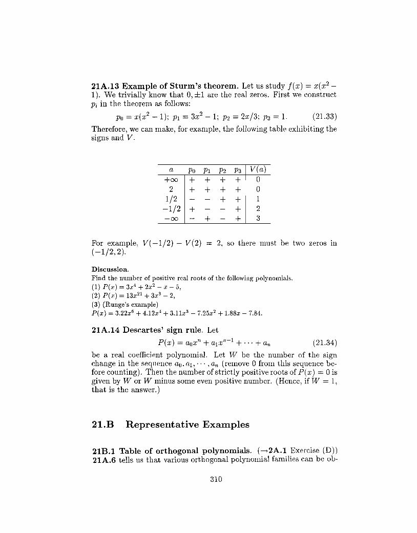
21A.13 Example of Sturm's theorem. Let us study f(x) = x(x21). We trivially know that 0, ±1 are the real zeros. First we constructPi in the theorem as follows:
Po = x(x2 - 1); PI = 3x2 - 1; P2 = 2x/3; P3 = 1. (21.33)
Therefore, we can make, for example, the following table exhibiting thesigns and V.
a Po PI P2 P3 V(a)+00 + + + + 0
2 + + + + 01/2 - - + + 1
-1/2 + - - + 2-00 - + - + 3
For example, V(-1/2) - V(2)(-1/2,2).
2, so there must be two zeros III
Discussion.Find the number of positive real roots of the following polynomials.(1) P(x) = 3x4 + 2x2 - x - 5,(2) P(x) = 13x21 +3x3
- 2,(3) (Runge's example)P(x) = 3.22x6 + 4.12x4 + 3.11x3
- 7.25x2 + 1.88x - 7.84.
21A.14 Descartes' sign rule. Let
P(x) = aoxn + al:Z;n-1 + ... + an (21.34)
be a real coefficient polynomial. Let W be the number of the signchange in the sequence ao, al," . ,an (remove 0 from this sequence before counting). Then the number of strictly positive roots of P(x) = 0 isgiven by War W minus some even positive number. (Hence, if ltV = 1,that is the answer.)
21.B Representative Examples
21B.l Table of orthogonal polynomials. (---t2A.l Exercise (D))21A.6 tells us that various orthogonal polynomial families can be ob-
310
tained by choosing wand s appropriately and also by choosing appropriate multiplicative numerical factors Kn • Some common examplesare given as follows.
name symbol domain w(x) s(x) K -1n
Legendre Pn [-1,1] 1 1 - x"l. (-1)n2nn!Chebychev Tn [-1,1] I/Vl - x2 1- x2 (-I)n(2n - I)!!
Jacobi p(o.f3) [-1,1] (1- x)Q(x + 1)f3 1 -x2 (-1)n2nn!n
Laguerre Ln [0,00) e x x n!Hermite Hn (-00,00) e-X- 1 (_1)n
Note that L n is L~O) of 2A.1.
Exercise. Show Tn = n!..;:rrp~-1/2.1/2) /f(n + 1/2).
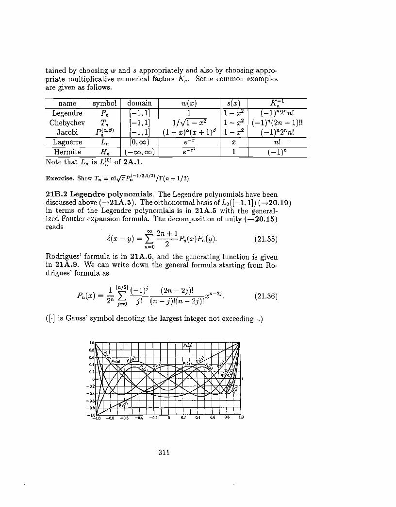
21B.2 Legendre polynomials. The Legendre polynomials have beendiscussed above (~21A.5). The orthonormal basis of L2([-I, 1]) (~20.19)in terms of the Legendre polynomials is in 21A.5 with the generalized Fourier expansion formula. The decomposition of unity (---+-20.15)reads
00 2n + 18(x - y) = L 2 Pn(x)Pn(y).
n=O(21.35)
(21.36)
Rodrigues' formula is in 21A.6, and the generating function is givenin 21A.9. We can write down the general formula starting from Rodrigues' formula as
1 [nJ2] (-I)j (2 - 2 ')'P ( ) = _ '" n J. n-2j
n X 2n f;:o j! (n _ j)!(n _ 2j)!x .
([.] is Gauss' symbol denoting the largest integer not exceeding .. )
LO p.(.) /'
0.8 ~)c~ .1 ....-'" I0.6 .\~p, (.) "?,0-...... ,I, ~'" ;'\ /0.4 I ~l)( /h ~r..........~ '><~b ~q,'t.102" ~)§. 1\ / 'j.\.. < I'-.. .-.?;...' ') ~ q,'" q,~ •
o \ '" v v?' ....... A ./ Ik-0.2 fI X ./ ~;:::::../ -f.--' 'V ........~)<~!l.~-0.4 .....-/ _ .......1--
-0.6 II I.A ,
I ....... '1'.,',\.,~_.1-I-t---4-1--1--l--+-+-l--+--+-+--+-t-t---l-0.8 v -t
10 .......- :"1.0 -0.8 -0.6 -0.4 0.2 0 0.2 0.4 0.6 0.8 1.0
311
Discussion.Let Qn(X) be the n-th order polynomial with its highest order coefficient normalizedto be unity. If its L 2-distance from 0 is the smallest among such polynomials, Qnis proportional to Pn . That is, minimize
(21.37)
with respect to the coefficients. The resultant polynomial is proportional to Pn .
21B.3 Sturm-Liouville equation for Legendre polynomials. Thedifferential equation corresponding to (21.16) reads (---t24C.l)
or
(21.38)
(21.39)
21BA Recursion formulas for Legendre polynomials. The threeterm recursion relation (---t21A.I0) reads
(21.40)
(21.41)
with Po (x) = 1 and P1(x) = x. This can also be obtained easily fromthe generating function (21.25): expand
? aw(1-2x(+(-)O( +(-(+x)w=O.
Similarly, we obtain
? aw(1 - 2x( +(-)- - (w = O.ax
This leads toP~+1 - 2xP~ + P~-l - Pn = O.
If we eliminate P~-l from (21.40) and (21.43), we get
P~+l - xP~ = (n + l)Pn .
If we eliminate P~+1 from (21.40) and (21.43), we get
xP~ - P~-l = nPn •
312
(21.42)
(21.43)
(21.44)
(21.45)
Combining above two formulas, we obtain
(21.46)
21B.5 Legendre polynomials, some properties.(1) Pn(x) is an odd (resp., even) function, if n is odd (resp., even):Pn(x) = (-l)npn(-x), Pn(1) = 1 and Pn(-l) = (_1)n. P2n (O) =(-;(2) (see Exercise below).
(2) IPn(x)1 :::; 1.(3) All the zeros of Pn are simple and in (-1,1) (-+21A.ll).(4) If I1n is an n-th order polynomial satisfying
(21.47)
for all k E {a, 1, ... ,n - I}, then I1n ex: Pn (-+21A.3(2»).[Demo of (2)] This can be proved with the aid of Schliifii's integral (21.23). Wechoose for the intergration path to be
t=z+~ei<l> (21.48)
for ep E [-1r, 1l"). Note that dt/ (t - z) = idep. Changing the integration variable fromt to ep in (21.23), we get the following Laplace's first integral
(21.49)
From this we get
ExerciseP2n(0) can be obtained from Rodrigues' formula (21.11), which reads
() (n r(n + 1/2)
P2n 0 = -1) J1rr(n + 1)'
(21.50)
(21.51)
21B.6 Hermite polynomials. The orthonormal basis {Ihn )} forL 2((-oo,oo),e- X2
) (-+20.19) obtained by the Gram-Schmidt methodapplied to monomials (-+21A.2) is written in terms of the Hermitepolynomials Hn(x) as
(21.52)
313
where
[(n+1)/2] ,Hn(x) = L (_)n . n. (2xt+1-2m.
m=O m!(n + 1 - 2m)!(21.53)
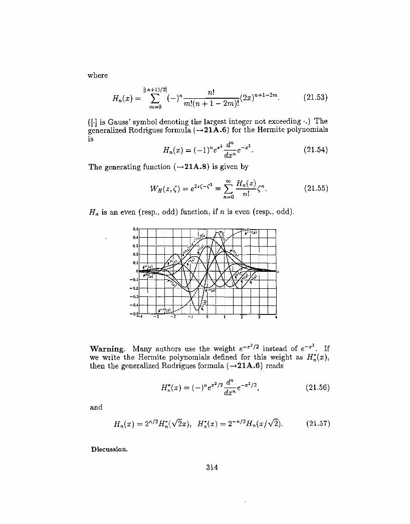
([.] is Gauss' symbol denoting the largest integer not exceeding '.) Thegeneralized Rodrigues formula (-+21A.6) for the Hermite polynomialsis
H ( ) - (_l)n x2 ..!!!:..- _x2
n X - e de.x n
The generating function (-+21A.8) is given by
(21.54)
W ( r) _ 2z(_(2 _ ~ Hn(z) rnHZ,., - e - L...J --,-" •
n=O n.(21.55)
H n is an even (resp., odd) function, if n is even (resp., odd).
3o
1M11~ "'~i-lIlz1r ,
~~,
V~'-.;f {7If... ,~~",
~;;.~!' \"-K
I t'J-j"\~"l(%l / \ X'~
~ \ A / X \ ~~~:J' ~z
;'''(z) \::I(,,)~ JI ~ .) __<..~vt4-.1
~ ...-;,/~
(Zl(x,
'\ h~1-'\%1. "
, \, ~
0.5
0.4
0.3
0.2
O.
o
-0.54
-0.2
-0.3
-0.4
-0.1
Warning. Many authors use the weight e-x2/2 instead of e-x2
• Ifwe write the Hermite polynomials defined for this weight as H~(x),
then the generalized Rodrigues formula (-+21A.6) reads
(21.56)
and
(21.57)
Discussion.
314
To demonstrate the completeness of the Hermite polynomials, Weierstrass' theorem 17.3 is not enough, because the latter is about a finite interval. To show thecompleteness with respect to the L 2-norm we have only to show the completenessof polynomials. This can be demonstrated with the aid of Weierstrass' theorem onincreasingly large intervals.
Exercise.(A) From the generating function show
ex'/2Hn(x) =~Joo eixv-v2/2Hn(y)dy.z V2ir -00
(21.58)
This can be split into real and imaginary part relations (Lebedev).(B) From the generating function we obtain the following generalized Fourier expansion
00 n
eax = ea' /4,""" _a_H (x) (21.59)L..t 2n , n ,o n.
which is good for all x E R.(C) Compute the generalized Fourier expansion of e-ax2 in terms of Hermite polynomials. The expansion coefficients can be written as
1 Joo ,_ -(a+l)x. .C2n - 22n (2n)!y'1r -00 e H2n (x)dx. (21.60)
To compute the integral use (21.69) below. The x-integration can be done and weare left with
( _l)TlaTl 100_ -8 n-l/2d
C2Tl - y'1r(2n)!(1 + a)Tl+l/2 0 e s s.
Use the Gamma function (-+9.6) to obtain the final result (Lebedev)
(_l)nan
(21.61)
(21.62)
21B.7 Sturm-Liouville equation for Hermite polynomials. Theformula corresponding to (21.16) reads
H~ - 2xH~ + 2nHn = 0. (21.63)
21B.8 Recurrence equations for Hermite polynomials. Thethree term recurrence relation (----+21A.I0) reads
Hn+l + 2xHn + 2nHn_1 = 0,
which can be obtained from
8WH8f = -2(z + Ow.
315
(21.64)
(21.65)
From
we obtain
f)WH = 2(wf)z
(21.66)
(21.67)
Exercise.An integral formula for Hermite polynomials can be obtained with the aid of
2 2 (Xi 2
e- X = -.[if Jo e- t cos2xtdt. (21.68)
[Hint. Note that the integrand is an even function.] Putting this into the generalizedRodrigues' formula (calculate the odd and even n cases separately, and unify theresults), we obtain
271( ')71 x
2 JooH ( ) - -z e -t 2+2itx "d
" x - r::::: e t t.y7r -00
(21.69)
21B.9 Chebychev polynomials. These polynomials are best introduced as
Tn(x) = cos(ncos-1 x).
The generalized Rodrigues formula (~21A.6) is given by
(21.70)
(21.71)
This can be transformed into (21.70) with the aid of the binomial theorem: it is easy to demonstrate that this formula yields
(21. 72)
which reduces to cos nO with x = cosO.The orthonormal basis {It n )} of L2([-1, 1], 1/Jl - x 2 )) (~20.19)
obtained by the Gram-Schmidt orthonormalization of monomials (~21A.6)can be written as
(xltn) = ~Tn(X).
The generating function (~21A.8) is
1 - z2 00
----=-2 = To(x) + 2 L: Tn(x)zn.1 - 2xz + Z 71=1
316
(21. 73)
(21.74)
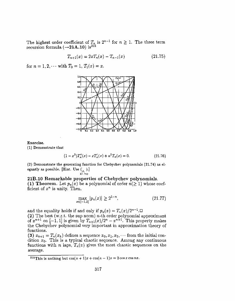
The highest order coefficient of Tn is 2n-
1 for n ~ 1. The three termrecursion formula (.....21A.10) is315
Tn+l(x) = 2xTn(x) - Tn-l(x)
for n = 1,2",' with To = 1, TI(x) = X.
Exercise.(1) Demonstrate that
(21.75)
(21.76)
(2) Demonstrate the generating function for Chebychev polynomials (21.74) as elegantly as possible. [Hint. Use (" ).]
:V.7Q
21B.10 Remarkable properties of Chebychev polynomials.(1) Theorem. Let Pn(x) be a polynomial of order n(~ 1) whose coefficient of xn is unity. Then,
max IPn(x)1 ~ 21-
n,
XE[-l,l](21.77)
and the equality holds if and only if Pn(x) =Tn(x)/2n- I .D(2) The best (w.r.t. the sup norm) n-th order polynomial approximantof xn+l on [-1,1] is given by Tn+l(x)/2n - xn+l. This property makesthe Chebychev polynomial very important in approximation theory offunctions.(3) Xk+l = Tn(Xk) defines a sequence Xo, Xl, X2,' .. from the initial condition xo. This is a typical chaotic sequence. Among any continuousfunctions with n laps, Tn(x) gives the most chaotic sequences on theaverage.
315This is nothing but cos(n + 1)x + cos(n - 1)x = 2 cosx cosnx.
317
Discussion.(A) (1) above implies that if the n-th order polynomial Qn defined on [-1,1] withits highest order coefficient normalized to be unity and if its maximum deviationfrom zero is the smallest among such polynomials, then Qn is proportional to theorder n Chebychev polynomial.(B) Take T2 (x). Demonstrate that there are two intervals I and J in [-1,1.] whichshare at most one point such that T2 (I) n T2 (J) :J I U J. In general, if the readercan find two positive integers and two intervals I and J sharing at most one pointsuch that reI) n fm(J) :J I U J, then f exhibits chaos on the inteval containingboth I and J. That is, there is an invariant set n of fN for some positive integerN such that fN restricted to n is isomorphic to the coin-tossing process.).
318
Related Documents