€¦ ·  · 2017-05-09Entrepreneurial Risk and Diversification through Trade Federico Esposito Tufts University May 2017 Abstract Demand shocks have been shown to be an important

Entrepreneurial Risk and Diversification throughTrade

Federico Esposito∗

Tufts University

May 2017

Abstract

Demand shocks have been shown to be an important determinant of firm sales’ variation across different markets.

In presence of incomplete financial markets or liquidity constraints, entrepreneurs may not be able to perfectly in-

sure against unexpected demand fluctuations. The key insight of this paper is that firms can reduce demand risk

through geographical diversification. I first develop a general equilibrium trade model with monopolistic compe-

tition, characterized by stochastic demand and risk-averse entrepreneurs, who exploit the imperfect correlation of

demand across countries to lower the variance of their total sales, in the spirit of classical portfolio analysis. The

model predicts that both entry and trade flows to a market are affected by its risk-return profile, which in turn de-

pends on the multilateral covariance of the country’s demand with all other markets. Moreover, welfare gains from

trade can be significantly higher than the gains predicted by standard models which neglect firm level risk. After a

trade liberalization, risk-averse firms boost exports to countries that offer better diversification benefits. Hence, in

these markets foreign competition becomes stronger, lowering the price level more. Therefore, countries with better

risk-return profiles gain more from international trade. I then use data on Portuguese firm-level international trade

flows, from 1995 to 2005, to provide evidence that exporters behave in a way consistent with my model’s predictions.

Finally, policy counterfactuals reveal that, for the median country, the risk diversification channel increases welfare

gains from trade by 15% relative to traditional models with risk neutrality.

∗Department of Economics, Tufts University, 8 Upper Campus Road, Medford, 02144, MA, USA. Email: [email protected]. I am extremely grateful to my advisor Costas Arkolakis, and to Lorenzo Caliendo, Samuel Kortum andPeter Schott for their continue guidance as part of my dissertation committee at Yale University. I thank the hospitality of the Eco-nomic and Research Department of Banco de Portugal where part of this research was conducted. I have benefited from discussionswith Treb Allen, Mary Amiti, David Atkin, Andrew Bernard, Kirill Borusyak, Arnaud Costinot, Penny Goldberg, Gene Grossman, TimKehoe, William Kerr, Giovanni Maggi, Monica Morlacco, Peter Neary, Luca Opromolla, Emanuel Ornelas, Michael Peters, TommasoPorzio, Vincent Rebeyrol, Steve Redding, Joe Shapiro, Robert Staiger, James Tybout as well as seminar participants at Yale University,Tufts University, SUNY Albany, Federal Reserve Board, University of Florida, Yale SOM, Bank of Italy, SED Toulouse, World Bank,AEA Meetings 2017, EEA Conference 2017, University of Naples. Finally, I thank Siyuan He and Guangbin Hong for excellent researchassistance. All errors are my own.

1 Introduction

Firms face substantial uncertainty about consumers’ demand. Recent empirical evidencehas shown that demand-side shocks explain a large fraction of the total variation of firmsales (see Fitzgerald et al. (2016), Hottman et al. (2015), Kramarz et al. (2014), Munchand Nguyen (2014), Eaton et al. (2011)).1 The role of demand uncertainty is particularlyimportant when firms must undertake costly irreversible investments, such as producinga new good or selling in a new market. However, in presence of incomplete financialmarkets or credit constraints, firms may not be able to perfectly insure against unexpecteddemand fluctuations.2

The key idea I put forward in this paper is that firms can hedge demand risk throughgeographical diversification. The intuition is that selling to markets with imperfectly cor-related demand can hedge against idiosyncratic shocks hitting sales. Although this sim-ple insight has always been at the core of the financial economics literature, starting fromthe seminal works by Markowitz (1952) and Sharpe (1964), the trade literature has so faroverlooked the risk diversification potential that international trade has for firms.3

In the first tier of my analysis, I develop a general equilibrium trade model with mo-nopolistic competition and heterogeneous firms, as in Melitz (2003) and Chaney (2008).The model is characterized by two novel elements. First, consumers have a ConstantElasticity of Substitution utility over a continuum of varieties, and demand is subjectto country-variety random shocks. In addition, for each variety these demand shocksare imperfectly correlated across countries. Second, firms are owned by risk-averse en-trepreneurs. This assumption reflects the evidence, discussed in Section 2, that most firmsacross several countries are owned by entrepreneurs whose wealth is not perfectly diver-sified and whose main source of income are their firm’s profits, therefore exposing theirincome to demand fluctuations.4 In addition, even for multinational and public listedfirms, whose ownership is not as concentrated as for small firms, stock-based compen-sation exposes their managers to firm-specific risk. Thus, in making economic decisionssuch as investment and production, managers reasonably attempt to minimize their riskexposure (see Ross (2004), Parrino et al. (2005) and Panousi and Papanikolaou (2012)).5

1See Section 2 for a thorough discussion of this evidence.2This may be the case especially in less developed countries (see Jacoby and Skoufias (1997), Greenwood

and Smith (1997) and Knight (1998)), and for small-medium firms (see Gertler and Gilchrist (1994) andHoffmann and Shcherbakova-Stewen (2011)).

3There are some recent exceptions, as Fillat and Garetto (2015) and Riaño (2011). See the discussionbelow.

4See Moskowitz and Vissing-Jorgensen (2002), Lyandres et al. (2013) and Herranz et al. (2015).5I assume that financial markets are absent. This assumption captures in an extreme way the incom-

pleteness of financial markets. Even if there were some financial assets available in the economy, as long as

1

The entrepreneurs’ problem consists of two stages. In the first stage, the entrepreneursknow only the moments of the demand shocks but not their realization. Firms make anirreversible investment: they choose in which countries to operate, and in these marketsperform costly marketing and distributional activities. After the investment in marketingcosts, firms learn the realized demand. Then, after uncertainty is resolved, entrepreneursfinally produce, using a production function linear in labor.6

The fact that demand is correlated across countries implies that, in the first stage, en-trepreneurs face a combinatorial problem. Indeed, both the extensive margin (whether toexport to a market) and the intensive margin (how much to export) decisions are interde-pendent across markets: any decision taken in a market affects the outcome in the others.Then, for a given number of potential countries N, the choice set includes 2N elements,and computing the indirect utility function corresponding to each of its elements wouldbe computationally unfeasible.7

I deal with this computational challenge by assuming that firms send costly ads ineach country where they want to sell. These activities allow firms to reach a fraction n ofthe consumers in each location, as in Arkolakis (2010).8 This implies that the firm’s choicevariable becomes continuous rather than discrete, and thus firms simultaneously choosewhere to sell (depending on whether n is optimally zero or positive) and how much to sell(firms can choose to sell to some or all consumers). In addition, the concavity of the firm’sobjective function, arising from the mean-variance specification, implies that the optimalsolution is unique.9

Therefore, the firm’s extensive and intensive margin decisions are not taken marketby market, but rather performing a global diversification strategy. Entrepreneurs tradeoff the expected global profits with their variance, the exact slope being governed by the

capital markets are incomplete firms would always be subject to a certain degree of demand risk. Shuttingdown financial markets therefore allows to focus only on international trade as a mechanism firms can useto stabilize their sales.

6The fact that companies cannot change the number of consumers reached after observing the shockshas an intuitive explanation. Investing in marketing activities is an irreversible activity, and thus very costlyto adjust after observing the realization of the shocks. An alternative interpretation of this irreversibilityis that firms sign contracts with buyers before the actual demand is known, and the contracts cannot berenegotiated.

7Other works in trade, such as Antras et al. (2014), Blaum et al. (2015), de Gortari et al. (2016) andMorales et al. (2014), deal with similar combinatorial problems, but in different contexts.

8As in Arkolakis (2010), firms incur in per-consumer marketing costs, paid in both domestic and foreignlabor.

9The presence of bounds in the firm’s problem (n cannot be negative and cannot be larger than 1)implies that I cannot solve the problem analytically. However, the concavity of the problem implies that,numerically, the firm’s problem can be solved using standard methods (such as the active set method)employed in quadratic programming problems with bounds. This is way faster than evaluating all thepossible combinations of extensive/intensive margin decisions.

2

risk aversion, along the lines of the “portfolio analysis” pioneered by Markowitz (1952)and Sharpe (1964).10 This stands in sharp contrast to standard trade models, such asMelitz (2003), Chaney (2008) and Helpman et al. (2008), where the decision to sell in onedestination is independent from the export decisions in other markets.

The model implies that both the probability of entering a market and the intensity oftrade flows are increasing in the market’s “Sharpe Ratio”.11 This variable measures thediversification benefits that a market can provide to firms exporting there. If demand ina country is relatively stable and negatively/mildly correlated with the rest of the world,then firms optimally choose, ceteribus paribus, to export more there to hedge their businessrisk. Therefore, my model suggests that neither the demand volatility in a market, northe bilateral covariance of demand with the domestic market, are sufficient to predict thedirection of trade. Instead, what determines trade patterns is the multilateral covariance:how much demand in a market co-varies with demand in other countries.

Furthermore, in a two-country version of the model, I show that the welfare gainsfrom international trade are increasing in the Sharpe Ratio.12 The intuition is simple: ifthe Sharpe Ratio is high, firms can hedge their domestic demand risk by exporting tothe foreign country. This implies tougher competition among firms, which in generalequilibrium leads to lower prices and higher welfare gains.13 Therefore, not only firmsare able to lower the volatility of their profits by diversifying their sales abroad, but theirrisk-hedging behavior has a “pro-competitive” effect on welfare.

In the second tier of my analysis, I rely on a panel dataset of Portuguese manufac-turing firms’ exports, from 1995 to 2005, to test the model’s predictions and to calibratethe model. Portugal is a small and export-intensive country, being at the 72nd percentileworldwide for exports per capita, and therefore can be considered a good laboratory toanalyze the implications of my model. Furthermore, 70% of Portuguese exporters in 2005were small firms, for which the exposure to demand risk is likely to be a first-order con-cern.

I first estimate the cross-country covariance matrix of demand, Σ. Given the staticnature of the model, Σ can be interpreted as a long-run covariance matrix that firms take

10The firms’ problem, however, is more involved than a standard portfolio problem, because it is subjectto bounds: the number of consumers reached in a destination can neither be negative nor greater than thesize of the population.

11Technically, the original Sharpe Ratio proposed by William Sharpe is the ratio between the mean andthe variance of an asset return, without taking into account for the covariance pattern with other assets.

12Given the complexity of the model, I can explicitly derive an expression for the welfare gains only inthe case of two symmetric countries.

13In my model, total welfare is the sum of workers’ welfare, which is simply the real wage, and en-trepreneurs’ welfare, which depends also on the variance of real profits.

3

as given when they choose their risk diversification strategy. Therefore, I estimate it byusing variation in firm-level exports to each destination over the years 1995-2004.14

From the estimated covariance matrix, I easily recover the Sharpe Ratios, the country-level measure of diversification benefits. I then test the prediction that the firms’ prob-ability of entry and trade flows to a market are increasing in the market’s Sharpe Ratio,using the Portuguese firm-level trade data for 2005. The findings confirm that, control-ling for several destination characteristics and “standard” gravity variables, e.g. bilateraldistance and tariffs, firms are more likely to enter in countries with high Sharpe Ratios,i.e. markets that provide good diversification benefits. Moreover, conditional on enteringa destination, firms export more to countries where they can better hedge their demandrisk.

In the second part of the empirical analysis, I calibrate the parameters of the model,which I augment with i) a non-tradeable sector; ii) intermediate inputs and iii) exoge-nous trade deficits, similarly to Caliendo and Parro (2014) and Arkolakis et al. (2015).15 Icalibrate the firms’ risk aversion by matching the observed (positive) gradient of the rela-tionship between the mean and the variance of firms’ profits, as suggested by the firm’sfirst order conditions.16 The reasoning is straightforward: if firms are risk-averse, theywant to be compensated for taking additional risk, and thus higher sales variance mustbe associated with higher expected revenues.17 Interestingly, the results suggest that amodest amount of risk aversion is sufficient to rationalize the magnitudes in the data.18

Lastly, I calibrate the remaining parameters, such as marketing and iceberg trade costs,with the Simulated Method of Moments, as in Eaton et al. (2011).19

Armed with the calibrated model, I quantify the risk diversification benefits of inter-national trade. Specifically, I follow Arkolakis et al. (2012) and Costinot and Rodriguez-Clare (2013) and compute the welfare gains of going from autarky, i.e. a world wheretrade costs are infinitely high, to the observed trade equilibrium in 2005. My results il-lustrate that countries with higher Sharpe Ratios benefit more from opening up to trade,

14There is evidence that, in the short run, firms sequentially enter different markets to learn their demandbehavior (see Albornoz et al. (2012) among others). In the data, this behavior may confound the pure riskdiversification behavior of exporters predicted by my model, affecting the estimation of Σ. Therefore, Iconsider only sales by “established” firm-destination pairs, i.e. exporters selling to a certain market for atleast 5 years. In this way, my estimates capture only the long run covariance of demand, rather than pickingalso some short-run noise due to the firms’ learning process.

15I also assume a Pareto distribution for firms productivity, as in Chaney (2008) and Arkolakis et al.(2008).

16As for the covariance estimation, I use firm-level data between 1995-2004.17Allen and Atkin (2016) use a similar approach to estimate the risk aversion of Indian farmers.18In addition, my estimate is close to the ones found by Allen and Atkin (2016) and Herranz et al. (2015).19In particular, I match the observed i) bilateral manufacturing trade shares; ii) normalized number of

Portuguese exporters to each destination; iii) mean and dispersion of export shares.

4

consistent with the theoretical results. The rationale is that firms exploit the trade liberal-ization not only to expand their sales abroad, but also to diversify their demand risk. Thisimplies that they optimally increase trade flows toward markets that provide better di-versification benefits, i.e. countries with a high Sharpe Ratio. Consequently, the increasein foreign competition is stronger in these countries, thereby lowering more prices.20

In addition, I compare the gains in my model with those predicted by traditional trademodels that neglect risk, as in Arkolakis et al. (2012) (ACR henceforth).21 My results showthat gains from trade are, for the median country, 15% higher than in ACR. Therefore,the “pro-competitive” effect of the firms’ risk diversification behavior is also quantita-tively relevant. However, while safer countries reap higher welfare gains than in ACR,markets with a worse risk-return profile have lower gains than in ACR, because the pro-competitive effect from foreign firms is weaker.

The result that some countries do not gain much from international trade, and couldpotentially lose from trade, is reminiscent of the result in Newbery and Stiglitz (1984). Intheir simple model with two sectors (one safe and one risky) and two countries, whenthere is free trade consumers are insured from the variance but prices go up (becauseproduction shifts toward the safe good), which can make countries worse off rather thanbetter off. A similar mechanism is at play in my model: although the variance of realprofits goes down, which makes firms better off, in risky countries the softer competitionfrom abroad could raise prices, thus lowering welfare.

This paper relates to the growing literature studying the importance of second ordermoments for international trade.22 Allen and Atkin (2015) use a portfolio approach tostudy the crop choice of Indian farmers under uncertainty. They show that greater tradeopenness increases farmers’ revenues volatility, leading farmers to switch to safer crops,which in turn increases their welfare. Similarly, in my model a trade liberalization in-duces firms to export more to less risky countries, which increases welfare gains througha general equilibrium force. Fillat and Garetto (2015) argue that multinational firms, dueto the large sunk costs of accessing foreign markets, are the most exposed to foreign de-mand risk, and therefore are riskier than firms selling domestically, especially in presenceof persistent disaster risk. While they focus on the link between a company’s interna-

20These findings are robust to the specification used for the entrepreneurs’ utility. In particular, I showthat having a decreasing rather than constant absolute risk aversion does not affect substantially the welfareresults.

21The models considered in ACR are characterized by (i) Dixit-Stiglitz preferences; (ii) one factor ofproduction; (iii) linear cost functions; and (iv) perfect or monopolistic competition. Among them, there arethe seminal papers by Eaton and Kortum (2002), Melitz (2003) and Chaney (2008).

22For earlier works, see Helpman and Razin (1978), Kihlstrom and Laffont (1979), Eaton and Grossman(1985) and Maloney and Azevedo (1995).

5

tional status and its stock return, I argue that international trade provides relevant riskdiversification benefits to exporters, especially small and medium ones. De Sousa et al.(2015) use a partial equilibrium model with risk averse firms to rationalize the empiricalfinding that volatility and skewness of demand affect the firms’ exporting decision. Mycontribution relative to these papers is, first, to establish that the multilateral covarianceof demand is a key driver of trade patterns, and then quantify the welfare benefits of riskdiversification, by means of a novel general equilibrium framework.23

This paper contributes to the literature that models exporters’ behavior. Previousmodels of firms’ export decision have studied a binary exporting decision (Roberts andTybout (1997); Das et al. (2007)) or have assumed that exporters make independent entrydecisions for each destination market (Helpman et al. (2008); Arkolakis (2010); Eaton et al.(2011)). In contrast, in my model entry in a given market depends on the global diversi-fication strategy of the firm and, despite the analytical complexity of the firm’s problem,I characterize both the extensive and intensive margin decisions.24 Another trade modelwhere the entry decision is interrelated across markets is Morales et al. (2015), in whichthe firm’s export decision depends on its previous export history.

My paper also complements the strand of literature that studies the connection be-tween openness to trade and macroeconomic volatility. Di Giovanni et al. (2014) inves-tigate how idiosyncratic shocks to large firms directly contribute to aggregate fluctua-tions, through input-output linkages across the economy. Caselli et al. (2012) show thatopenness to international trade can lower GDP volatility by reducing exposure to domes-tic shocks and allowing countries to diversify the sources of demand and supply acrosscountries. My paper, in contrast, investigates the implications of firm-level demand riskfor international trade patterns and aggregate welfare.

Finally, my paper connects to the literature that studies the implications of incompletefinancial markets for entrepreneurial risk and firms’ behavior and performance. Herranzet al. (2015) show, using data on ownership of US small firms, that entrepreneurs arerisk-averse and hedge business risk by adjusting the firm’s capital structure and scale ofproduction. Other notable contributions to this literature are Heaton and Lucas (2000),Roussanov (2010), Luo et al. (2010), Chen et al. (2010) and Hoffmann (2014).

23Other recent works exploring the link between uncertainty and trade are Koren (2003), Rob and Vettas(2003), Di Giovanni and Levchenko (2010), Riaño (2011), Nguyen (2012), Impullitti et al. (2013), Vannooren-berghe (2012), Ramondo et al. (2013), Vannoorenberghe et al. (2014), Novy and Taylor (2014) and Gervais(2016).

24 Heiland (2016) and De Sousa et al. (2015) also feature risk averse exporters, but the extensive margindecision is not modeled.

6

The remainder of the paper is organized as follows. Section 2 presents some stylizedfacts that corroborate the main assumptions of the model, presented in Section 3. In Sec-tion 4, I estimate the model and empirically test its implications. In Section 5, I perform anumber of counterfactual exercises. Section 6 concludes.

2 Motivating evidence

Compared to standard trade models, such as Melitz (2003), the main novelty of my frame-work is that entrepreneurs are risk averse. There is recent evidence supporting this as-sumption. Cucculelli et al. (2012) survey several Italian entrepreneurs in the manufac-turing sector and show that 76.4% of interviewed decision makers are risk averse. In-terestingly, larger firms tend to be managed by decision makers with lower risk aver-sion.25 A survey promoted by the consulting firm Capgemini reveals that, among 300managers/CEO of leading companies across several countries, 40% of them believes thatmarket/demand volatility is the most important challenge for their firm.26 Further ev-idence that entrepreneurs display a risk-averse behavior has been recently provided, indifferent contexts, by Herranz et al. (2015), De Sousa et al. (2015) and Allen and Atkin(2016).

It is important to note that risk aversion is a factor affecting the behavior of largefirms/multinationals as well, not just small-medium enterprises. Indeed, risk aversionarises if corporate management seeks to avoid default risk and the costs of financial dis-tress, where these costs rise with the variability of the net cash flows of the firm (see Frootet al. (1993) and Allayannis et al. (2008)). Moreover, stock-based compensation exposesmanagers to firm-specific risk (see Petersen and Thiagarajan (2000), Ross (2004), Parrinoet al. (2005) and Panousi and Papanikolaou (2012)). Thus, in making economic decisionssuch as investment and production, managers reasonably attempt to minimize their riskexposure.

Two objections could be raised to the risk aversion assumption. The first is that en-trepreneurs could invest their wealth across several assets, diversifying away businessrisk. In reality, however, the majority of firms around the globe are controlled by imper-fectly diversified owners. Using a dataset about ownership of 162,688 firms in 34 European

25I will take into account for these differences in risk aversion in an extension of the model.26This survey was conducted in 2011 among 300 companies from Europe (59%), the US and Canada

(25%), Asia-Pacific (10%) and Latin America (6%). The survey can be found here: https://www.capgemini-consulting.com/resource-file-access/resource/pdf/The_2011_Global_Supply_Chain_Agenda.pdf.

7

countries, Lyandres et al. (2013) show that entrepreneurs’ holdings are far from beingwell-diversified.27 The median entrepreneur in their sample owns shares of only twofirms, and the Herfindhal Index of his holdings is 0.67, a number indicating high con-centration of wealth.28 According to the Survey of Small Business Firms (2003), a largefraction of US small firms’ owners invest substantial personal net-worth in their firms:half of them have 20% or more of their net worth invested in one firm, and 87% of themwork at their company.29 Moreover, Moskowitz and Vissing-Jorgensen (2002) estimatethat US households with entrepreneurial equity invest on average more than 70 percentof their private holdings in a single private company in which they have an active man-agement interest.30

The second objection that could be raised is that firms can hedge demand risk onfinancial and credit markets. However, often small firms (which account for the vast ma-jority of existing firms) have a limited access to capital markets (see Gertler and Gilchrist(1994), Hoffmann and Shcherbakova-Stewen (2011)), and even large firms under-invest infinancial instruments (see Guay and Kothari (2003)) and, when they do, such instrumentsoften do not successfully reduce risks (see Hentschel and Kothari (2001)).31 In addition,notice that financial derivatives can be used to hedge interest rate, exchange rate, andcommodity price risks, rather than demand risk, which is the focus of this paper.

The model also features country-variety demand shocks. Recent empirical evidencehas shown that demand shocks explain a large fraction of the total variation of firm sales.Hottman et al. (2015) have shown that 50-70 percent of the variance in firm sales can beattributed to differences in firm appeal. Eaton et al. (2011) and Kramarz et al. (2014) withFrench data and Munch and Nguyen (2014) with Danish data have instead estimatedthat firm-destination idiosyncratic shocks drive around 40-45% percent of sales varia-

2796% of firms in their sample are privately-held. They use three measures of diversification of en-trepreneurs’ holdings: i) total number of firms in which the owner holds shares, directly or indirectly; ii)Herfindhal index of firm owner’s holdings; iii) the correlation between the mean stock return of publicfirms in the firm’s industry and the shareholder’s overall portfolio return.

28There is a growing body of theoretical literature that explains this concentration of entrepreneurs’portfolios and thus their exceptional role as owners of equity. See Carroll (2002), Roussanov (2010), Luoet al. (2010) and Chen et al. (2010).

29This Survey, administered by Federal Reserve System and the U.S. Small Business Administration,is a cross sectional stratified random sample of about 4,000 non-farm, non-financial, non-real estate smallbusinesses that represent about 5 million firms.

30Similar evidence that companies are controlled by imperfectly diversified owners has been providedby Benartzi and Thaler (2001), Agnew et al. (2003), Heaton and Lucas (2000), Faccio et al. (2011) and Herranzet al. (2013).

31Hentschel and Kothari (2001), using data from financial statements of 425 large US corporations findthat many firms manage their exposures with large derivatives positions. Nonetheless, compared to firmsthat do not use financial derivatives, firms that use derivatives display few, if any, measurable differencesin risk that are associated with the use of derivatives.

8

tion. Recent contributions also include Bricongne et al. (2012), Nguyen (2012), Munch andNguyen (2014), Berman et al. (2015) and Armenter and Koren (2015). Di Giovanni et al.(2014) show that firm-specific components account for the vast majority of the variation insales growth rates across firms, the remaining being sectoral and aggregate shocks. In ad-dition, about half of the variation in the firm-specific component is explained by variationin that component across destinations.

The insight of this paper is that risk averse entrepreneurs optimally hedge these id-iosyncratic demand shocks by exporting to markets with imperfectly correlated shocks. Inthe following section I describe the theoretical framework, where I introduce entrepreneurs’risk aversion and correlated demand shocks in a general equilibrium trade model, andshow their implications trade patterns and welfare gains from trade.

3 A trade model with risk-averse entrepreneurs

I consider a static trade model with N asymmetric countries. The importing market isdenoted by j, and the exporting market by i, where i, j = 1, ..., N. Each country j ispopulated by a continuum of workers of measure Lj, and a continuum of risk-averse en-trepreneurs of measure Mj. Each entrepreneur owns a non-transferable technology toproduce, with productivity z, a differentiated variety under monopolistic competition,as in Melitz (2003) and Chaney (2008). The productivity z is drawn from a known dis-tribution, independently across countries and firms, and its realization is known by theentrepreneurs at the time of production. Since there is a one-to-one mapping from theproductivity z to the variety produced, throughout the rest of the paper I will always usez to identify both. Finally, I assume that financial markets are absent.32

3.1 Consumption side

Both workers and entrepreneurs have access to a potentially different set of goods Ωij.Each agent υ chooses consumption by maximizing a CES aggregator of a continuum num-ber of varieties, indexed with z:

32This assumption captures in an extreme way the incompleteness of financial markets. Even if therewere some financial assets available in the economy, as long as capital markets are incomplete firms wouldalways be subject to a certain degree of demand risk. Shutting down financial markets therefore allows tofocus only on international trade as a mechanism firms can use to stabilize their sales. See also Riaño (2011)and Limão and Maggi (2013).

9

max Uj(υ) =

(∑

i

∫Ωij

αj(z)1σ qj(z, υ)

σ−1σ dz

) σσ−1

(1)

s.to ∑i

∫Ωij

pj(z)qj(z, υ)dz ≤ y(υ) (2)

where y(υ) is agent υ’s income, and σ > 1 is the elasticity of substitution across vari-eties. Although the consumption decision, given income y(υ), is the same for workers andentrepreneurs, their incomes differ. In particular, workers earn labor income by working(inelastically) for the entrepreneurs. I assume that there is perfect and frictionless mobil-ity of workers across firms, and therefore they all earn the same non-stochastic wage w.In contrast, entrepreneurs’ only source of income are the profits they reap from operatingtheir firm. Entrepreneurs, therefore, own a technology to maximize their income, but theyincur in business risk, as it will be clearer in the next subsection.

The term αj(z) reflects an exogenous demand shock specific to good z in market j,similarly to Eaton et al. (2011), Nguyen (2012) and Di Giovanni et al. (2014). This is theonly source of uncertainty in the economy. Define α(z) ≡ α1(z), ...αN(z) to be the vectorof realizations of the demand shock for variety z. I assume that:

Assumption 1. α(z) ∼ G (α, Σ), i.i.d. across z

Assumption 1 states that the demand shocks are drawn, independently across vari-eties, from a multivariate distribution characterized by an N-dimensional vector of meansα and an N × N variance-covariance matrix Σ. Given the interpretation of αj(z) as a con-sumption shifter, I assume that the distribution has support over R+.

Few comments are in order. First, by simply specifying a generic covariance matrixΣ, I am not making any restrictions on the cross-country correlations of demand, whichtherefore can range from -1 to 1. Second, I assume that these shocks are variety specific.Therefore I am ruling out, for the moment, any aggregate shocks that would affect thedemand for all varieties. Third, for simplicity I assume that the moments of the shocksare the same for all varieties, but it would be fairly easy to extend the model to haveG (α, Σ) varying across sectors.

The maximization problem implies that the agent υ’s demand for variety z is:

qj(z, υ) = αj(z)pj(z)−σ

P1−σj

yj(υ), (3)

10

where pj(z) is the price of variety z in j, and Pj is the standard Dixit-Stiglitz price index. Inequation 3, the demand shifter αj(z) can reflect shocks to preferences, climatic conditions,consumers confidence, regulation, firm reputation, etc. (see also De Sousa et al. (2015)).

3.2 Production side

Entrepreneurs are the only owners and managers of their firms, and their only sourceof income are their firm’s profits. Alternatively, we can think of them as the majorityshareholders of their firm, with complete power over the firm’s production choices. Thisassumption captures, in an extreme way, the evidence shown earlier that the majority ofentrepreneurs around the globe do not have a well-diversified wealth. They choose howto operate their firm z in country i by maximizing the following indirect utility in realincome:

max V(

yi(z)Pi

)= E

(yi(z)

Pi

)− γ

2Var

(yi(z)

Pi

)(4)

where yi(z) equals net profits. The mean-variance specification above can be derived as-suming that the entrepreneurs maximize an expected CARA utility in real income (seeEeckhoudt et al. (2005)).33 The CARA utility has been widely used in the portfolio allo-cation literature (see, for example, Markowitz (1952), Sharpe (1964) and Ingersoll (1987)),and has the advantage of having a constant absolute risk aversion, given by the parame-ter γ > 0, which gives a lot of tractability to the model. One shortcoming of the CARAutility is that the absolute risk aversion is independent from wealth. In the Appendix Iconsider a variation of the model where the entrepreneurs have a CRRA utility, and thusa decreasing absolute risk aversion, and show that the overall implications do not changesubstantially.

The production problem consists of two stages. In the first, firms know only the dis-tribution of the demand shocks, G(α), but not their realization. Under uncertainty aboutfuture demand, firms make an irreversible investment: they choose in which countriesto operate, and in these markets perform costly marketing and distributional activities.After the investment in marketing costs, firms learn the realized demand. Then, en-trepreneurs produce using a production function linear in labor, and allocate their real

33If the entrepreneurs have a CARA utility with parameter γ, a second-order Taylor approximation ofthe expected utility leads to the expression in 4 (see Eeckhoudt et al. (2005) and De Sousa et al. (2015) for astandard proof). If the demand shocks are normally distributed, the expression in 4 is exact (see Ingersoll(1987)).

11

income to different consumption goods, according to the sub-utility function in 1.34

I assume that the first stage decision cannot be changed after the demand is observed.This assumption captures the idea that marketing activities present irreversibilities thatmake reallocation costly after the shocks are realized.35 An alternative interpretation ofthis irreversibility is that firms sign contracts with buyers before the actual demand isknown, and the contracts cannot be renegotiated.

The fact that demand is correlated across countries implies that, in the first stage, en-trepreneurs face a combinatorial problem. Indeed, both the extensive margin (whether toexport to a market) and the intensive margin (how much to export) decisions are inter-twined across markets: any decision taken in a market affects the outcome in the others.Then, for a given number of potential countries N, the choice set includes 2N elements,and computing the indirect utility function corresponding to each of its elements wouldbe computationally unfeasible.36

I deal with such computational challenge by assuming that firms send costly ads ineach country where they want to sell. These activities allow firms to reach a fractionnij(z) of consumers in location j, as in Arkolakis (2010).37 This implies that the firm’schoice variable is continuous rather than discrete, and thus firms simultaneously choosewhere to sell (if nij(z) is optimally zero, firm z does not sell in country j) and how much tosell (firms can choose to sell to some or all consumers). In addition, the concavity of thefirm’s objective function, arising from the mean-variance specification, implies that theoptimal solution is unique, as I prove in Proposition 1 below.

The fact that the ads are sent independently across firms and destinations, and theexistence of a continuum number of consumers, imply that the total demand for varietyz in country j is:

qij(z) = αj(z)pij(z)−σ

P1−σj

nij(z)Yj, (5)

where Yj is the total income spent by consumers in j, and Pj is the Dixit-Stiglitz priceindex:

34See Koren (2003) for a similar configuration of the production structure.35For a similar assumption, but in different settings, see Ramondo et al. (2013), Albornoz et al. (2012)

and Conconi et al. (2016).36Other works in trade, such as Antras et al. (2014), Blaum et al. (2015) and Morales et al. (2014), deal

with similar combinatorial problems, but in different contexts.37Estimates of marketing costs (see Barwise and Styler (2003), Butt and Howe (2006) and Arkolakis

(2010)) indicate that the amount of marketing spending in a certain market is between 4 to 7.7% of GDP.

12

P1−σj ≡∑

i

∫Ωij

nij(z)αj(z)(

pij(z))1−σ dz. (6)

Therefore, the first stage problem is to choose nij(z) to maximize the following:

maxnij∑j

E(

πij(z)Pi

)− γ

2 ∑j

∑s

Cov(

πij(z)Pi

,πis(z)

Pi

)(7)

s. to 1 ≥ nij(z) ≥ 0 (8)

where πij(z) are net profits from destination j:

πij(z) = qij(nij(z))pij(z)− qij(nij(z))τijwi

z− fij(z), (9)

and τij ≥ 1 are iceberg trade costs and fij are marketing costs.38 In particular, I assumethat there is a non-stochastic cost, f j > 0, to reach each consumer in country j, and thatthis cost is paid in both domestic and foreign labor, as in Arkolakis (2010).39 Thus, totalmarketing costs are:

fij(z) = wβi w1−β

j f jLjnij(z). (10)

where Lj ≡ Lj + Mj is the total measure of consumers in country j, and β > 0.40

The bounds on nij(z) in equation (8) are a resource constraint: the number of con-sumers reached by a firm cannot be negative and cannot exceed the total size of the pop-ulation. Using finance jargon, a firm cannot “short” consumers (nij(z) < 0) or “borrow”them from other countries (nij(z) > 1). This makes the maximization problem in (7) quitechallenging, because it is subject to 2N inequality constraints. In finance, it is well knownthat there is no closed form solution for a portfolio optimization problem with lower andupper bounds (see Jagannathan and Ma (2002) and Ingersoll (1987)).

Notice that the variance of global real profits is the sum of the variances of the profitsreaped in all potential destinations. In turn, these variances are the sum of the covariancesof the profits from j with all markets, including itself. If the demand shocks were not

38I normalize domestic trade barriers to τii = 1, and I further assume τij ≤ τivτvj for all i, j, v to excludethe possibility of transportation arbitrage.

39Sanford and Maddox (1999) provide evidence that exporters use foreign advertising agencies, andLeonidou et al. (2002) review some direct evidence of the use of domestic labor for foreign advertising.

40In accordance with Arkolakis (2010), I will make specific assumptions on f j in the calibration section.However, the fact that f j does not depend on nij(z) means that the marginal cost of reaching an additionalconsumer is constant, which is a special case of Arkolakis (2010).

13

correlated across countries, then the objective function would simply be the sum of theexpected profits minus the variances.

The assumption that the shocks are independent across a continuum of varieties im-plies that aggregate variables wj and Pj are non-stochastic. Therefore, plugging into πij(z)the optimal consumers’ demand from equation (5), I can write expected profits more com-pactly as:

E(πij(z)

)= αjnij(z)rij(z)−

1Pi

fij(z), (11)

where αj is the expected value of the demand shock in destination j, and

rij(z) ≡1Pi

Yj pij(z)−σ

P1−σj

(pij(z)−

τijwi

z

). (12)

Note that nij(z)rij(z) are real gross profits in j. Similarly, the covariance between πij(z)and πis(z) is simply:

Cov(

πij(z)Pi

,πis(z)

Pi

)= nij(z)rij(z)nis(z)ris(z)Cov(αj, αs), (13)

where Cov(αj, αs) is the covariance between the shock in country j and in country s.41

Although there is no analytical solution to the first stage problem, because of the pres-ence of inequality constraints, we can take a look at the firm’s interior first order condition:

rij(z)αj − γrij(z)∑s

nis(z)ris(z)Cov(αj, αs)︸ ︷︷ ︸marginal benefit

=1Pi

wβi w1−β

j f jLj︸ ︷︷ ︸marginal cost

. (14)

Equation (14) equates the real marginal benefit of adding one consumer to its real marginalcost. While the marginal cost is constant, the marginal benefit is decreasing in nij(z). Inparticular, it is equal to the marginal revenues minus a “penalty” for risk, given by thesum of the covariances that destination j has with all other countries (including itself).The higher the covariance of market j with the rest of the world, the smaller the diversifi-cation benefit the market provides to a firm exporting from country i.

An additional interpretation is that a market with a high covariance with the rest of theworld must have high average real profits to compensate the firm for the additional risk

41The covariance does not depend on the marketing costs because these are non-stochastic.

14

taken: this trade-off between risk and return is determined by the degree of risk aversion.I will indeed use this intuition to calibrate the risk aversion parameter in the data.

Note the difference in the optimality condition with Arkolakis (2010). In his paper,the marginal benefit of reaching an additional consumer is constant, while the marginalpenetration cost is increasing in nij(z). In my setting, instead, the marginal benefit ofadding a consumer is decreasing in nij(z), due to the concavity of the utility function ofthe entrepreneur, while the marginal cost is constant.

To find the general solution for nij and pij, I only need to make the following assump-tion, which I assume will hold throughout the paper:

Assumption 2. det(Σ) > 0

Assumption 2 is a necessary and sufficient condition to have uniqueness of the op-timal solution. Since Σ is a covariance matrix, which by definition always has a non-negative determinant, this assumption simply rules out the knife-edge case of a zero de-terminant.42 In the Appendix, I prove that (dropping the subscripts i and z for simplicity):

Proposition 1. For firm z from country i, the unique vector of optimal n satisfies:

n =1γ

Σ−1 [π − µ + λ] , (15)

where Σ is firm z’s matrix of profits covariances, π is the vector of expected net profits, µ and λ

are the vectors of Lagrange multipliers associated with the bounds.Moreover, the optimal price charged in destination j is a constant markup over the marginal

cost:

pij(z) =σ

σ− 1τijwi

z(16)

Proposition 1 shows that the optimal solution, as expected, resembles the standardmean-variance optimal rule, which dictates that the fraction of wealth allocated to eachasset is proportional to the inverse of the covariance matrix times the vector of expectedexcess returns (see Ingersoll (1987) and Campbell and Viceira (2002)). The novelty of thispaper is that such diversification concept is applied to the problem of the firm. The en-trepreneurs, rather than solving a maximization problem country by country, as in tradi-

42A zero determinant would happen only in the case where all pairwise correlations are exactly 1.

15

tional trade models, perform a global diversification strategy: they trade off the expectedglobal profits with their variance, the exact slope being governed by the absolute degreeof risk aversion γ > 0.

Note that the firm’s entry decision in a market (that is, whether n > 0) does not dependon a market-specific entry cutoff, but rather on the global diversification strategy of thefirm. Therefore, the fact that a firm with productivity z1 enters market j, i.e. nij(z1) > 0,does not necessarily imply that a firm with productivity z2 > z1 will enter j as well. For ex-ample, a small firm may enter market j because it provides a good hedge from risk, whilea larger firm does not enter j since it prefers to diversify risk by selling to other markets,where the small firm is not able to export. This is a novel feature of my model, and itdiffers from traditional trade models with fixed costs, such as Melitz (2003) and Chaney(2008), where the exporting decision is strictly hierarchical. Recent empirical evidence(see Bernard et al. (2003), Eaton et al. (2011) and Armenter and Koren (2015)) suggestsinstead that, although exporters are more productive than non-exporters in general, thereare firms which are more productive than exporters but that still only serve the domesticmarket.

Finally, since the pricing decision is made after the uncertainty is resolved, and for agiven nij(z), the optimal price follows a standard constant markup rule over the marginalcost, shown in equation 16. Therefore, the realization of the shock in market j only shiftsupward or downward the demand curve, without changing its slope.

A limit case. It is worth looking at the optimal solution in the special case of riskneutrality, i.e.γ = 0. In the Appendix I show that, in this case, a firm sells to countryj only if its productivity exceeds an entry cutoff:

(zij)σ−1

=wβ

i w1−βj f jLjP1−σ

j σ

αj(

σσ−1 τijwi

)1−σ Yj, (17)

and that, whenever the firm enters a market, it sells to all consumers, so that nij(z) = 1.This case is isomorphic (with αj = 1) to the firm’s optimal behavior in trade models withrisk-neutrality and fixed entry costs, such as Melitz (2003) and Chaney (2008). In thesemodels, firms enter all profitable locations, i.e. the markets where the revenues are higherthan the fixed costs of production, and upon entry they serve all consumers.43 The caseof γ = 0 constitutes an important benchmark, as I will compare the welfare impact ofcounterfactual policies in my model with a positive risk aversion versus a model with

43Even in models with endogenous marketing costs, such as Arkolakis (2010), firms may not reach allconsumers in a destination, but they enter only if the productivity is larger than an entry cutoff.

16

γ = 0, i.e. the canonical trade models by Melitz (2003), Chaney (2008).

3.2.1 Trade patterns

To gain more intuition from Proposition 1, let us ignore for a moment the inequalityconstraints in the firm problem. Then, equation (15) becomes:

nij(z) =Sj

rij(z)γ−

∑k Cjkwi fk Lkrik(z)

rij(z)γ, (18)

where Sj is the Sharpe Ratio of country j:

Sj ≡∑k

Cjkαj (19)

and Cjk is the j− k cofactor of the covariance matrix of demand Σ.44 The Sharpe Ratio inequation (19) is an (inverse) measure of country risk. For example, with two symmetriccountries, Sj equals:

S =α

σ2(1 + ρ), (20)

where σ2 and α denote the variance and the mean of the demand shocks, respectively, andρ is the cross-country correlation. Equation (20) shows that the Sharpe Ratio is decreasingin the volatility of the shocks, and decreasing in the correlation of demand with the othercountry.45 In the general case of N countries, i.e. equation (19), it is easily verifiable thatSj is decreasing in the variance of demand in market j and in the correlation of demandin j with the rest of the world. The intuition is that the more volatile demand in market j,relative to its mean, or the more demand is correlated with the rest the world, the riskieris country j, and the lower Sj. Therefore the Sharpe Ratio summarizes the diversificationbenefits that a country provides to firms, since it is inversely proportional to the overallriskiness of its demand.

Then, equation (18) implies that both the probability of exporting to a country and thenumber of consumers reached are increasing in the Sharpe Ratio, holding constant wages

44The cofactor is defined as Ckj ≡ (−1)k+j Mkj, where Mkj is the (k, j) minor of Σ. The minor of a matrixis the determinant of the sub-matrix formed by deleting the k-th row and j-th column.

45Recall that the Sharpe Ratio of a stochastic variable is defined as the ratio of its expected mean (orsometimes its “excess” expected return over the risk-free rate) over its standard deviation (or sometimesthe variance).

17

and prices.46 Thus, a firm is more likely to enter a market with a higher Sharpe Ratio,i.e. a market that provides good diversification benefits, conditional on trade barriersand market specific characteristics. In addition, conditional on entering a destination, theamount exported is larger in markets with high Sharpe Ratio. The intuition is that, if amarket is “safe”, then firms optimally choose to be more exposed there to hedge theirbusiness risk, and thus export more intensely to that market.

In the Appendix, I prove that this result holds also in the general case where someinequality constraints are binding, i.e. the firm does not enter all markets:

Proposition 2. Define A a matrix whose i− j element equals Aij = −∑k 6=1 CikCov(αk, αj) fori 6= j, and Aij = 1 for i = j. If A is a M-matrix, then the probability of exporting and the amountexported to a market are increasing in its Sharpe Ratio.

Proposition 2 suggests that neither the demand volatility in a market, nor the bilateralcovariance of demand with the domestic market, are sufficient to predict the directionof trade. Instead, what determines trade patterns is the multilateral covariance, i.e. howmuch the demand in a market co-varies with demand in all other countries. The sufficient,but not necessary, condition to have a positive effect of the Sharpe Ratio on nij(z) is thatthe matrix A is a M-matrix, i.e. all off-diagonal elements are negative. It is easy to verifythat A is a M-matrix whenever some demand correlations are negative.47

Propositions 1 and 2 also suggest how my model can reconcile the positive relation-ship between firm entry and market size with the existence of many small exporters ineach destination, as shown by Eaton et al. (2011) and Arkolakis (2010). On one hand,upon entry firms can extract higher profits in larger markets. Therefore, more companiesenter markets with larger population size. On the other hand, the firms’ global diversifi-cation strategy may induce them to optimally reach only few consumers, and thus exportsmall amounts. In contrast, the standard fixed cost models, such as Melitz (2003) andChaney (2008), require large fixed costs to explain firm entry patterns, which contradictthe existence of many small exporters. In the empirical section, I will use this feature totest the model’s goodness of fit in the data.

Having characterized the exporting behavior of risk averse firms, I now define the

46Note that if the Sharpe Ratio of a country changes because of a shock to the covariance matrix, thatwill have also a general equilibrium effect on wages and prices. In Proposition 2, I focus on the partialequilibrium effect of the Sharpe Ratio on the firm decision. The prediction, however, holds true also ingeneral equilibrium, as I show in the counterfactual analysis in Section 5.

47This can be seen, for example, for the case N = 4, where a typical element of the matrix A looks like:

A21 = ρ12σ31 σ2σ2

3 σ24 (1− ρ2

13 − ρ214 − ρ2

34 + 2ρ13ρ14ρ34).

Then, to have A21 < 0, at least one correlation needs to be negative.

18

world equilibrium and discuss its properties.

3.3 General equilibrium

I now describe the equations that define the trade equilibrium of the model. FollowingHelpman et al. (2004), Chaney (2008) and Arkolakis et al. (2008), I assume that the produc-tivities are drawn, independently across firms and countries, from a Pareto distributionwith density:

g(z) = θz−θ−1, z ≥ z, (21)

where z > 0. The price index is:

P1−σi = ∑

jMj

∫ ∞

zαinji(z)pji(z)1−σg(z)dz, (22)

where nji(z) and pji(z) are given in Proposition 1.48 Since the optimal fraction of con-sumers reached, nij(z), is bounded between 0 and 1, a sufficient condition to have a finiteintegral is that θ > σ− 1. As in Chaney (2008), the number of firms is fixed to Mi, imply-ing that in equilibrium there are profits, which equal:

Πi = Mi ∑j

(1σ

∫ ∞

zαj qij(z)pij(z)g(z)dz−

∫ ∞

zfij(z)g(z)dz

). (23)

where qij(z) is the non-stochastic part of demand.49 I impose a balanced current account,thus the sum of labor income and business profits must equal the total income spent inthe economy:

Yi = wi Li + Πi. (24)

Finally, the labor market clearing condition states that in each country the supply of labormust equal the amount of labor used for production and marketing:

Mi ∑j

∫ ∞

z

τij

zαj qij(z)g(z)dz + Mi ∑

j

∫ ∞

zf jnij(z)Ljg(z)dz = Li, (25)

48The assumptions that the demand shocks are i.i.d. across a continuum of varieties, and that the meanof the shocks is the same for all z, imply that in the expression for the price index there is simply αi =αi(z) ≡

∫ ∞0 αi(z)gi(α)dα, where gi(α) is the marginal density function of the demand shock in destination

i.49Specifically, qij =

pij(z)−σ

P1−σj

nij(z)Yj.

19

Therefore the trade equilibrium in this economy is characterized by a vector of wageswi, price indexes Pi and income Yi that solve the system of equations (22), (24),(25), where nij is given by equation (15).50 It is worth noting that the realization of thedemand shocks does not affect the equilibrium wages and prices, because on aggregatethe idiosyncratic shocks average out by the Law of Large Numbers.51

Proposition 1 implies that the sales of firm z to country j are given by:

xij(z) = pij(z)qij(z) = αj(z)(

σ

σ− 1τijwi

z

)1−σ Yj

P1−σj

nij(z) (26)

where nij(z) satisfies equation (15). From equation (26), aggregate trade flows from i to jare:

Xij = Mi

∫ ∞

zαj

(σ

σ− 1τijwi

z

)1−σ Yj

P1−σj

nij(z)θz−θ−1dz. (27)

Proposition 2 then implies that aggregate trade flows Xij are increasing in Sj, the mea-sure of diversification benefits that destination j provides to exporters. I will test thisprediction in the data.

3.4 Welfare gains from trade

I define welfare in country i as the equally-weighted sum of the welfare of workersand entrepreneurs:

Wi = Uwi Li + Mi

∫ ∞

zUe

i (z) dG(z), (28)

where Uwi is the indirect utility of each worker (which is the same for all workers), while

Ue (z) is the indirect utility of each entrepreneur (which differs depending on the produc-tivity z). Since workers maximize a CES utility, their welfare is simply the real wage wi

Pi, as

in ACR. In contrast, the entrepreneurs maximize a stochastic utility, and thus the correctmoney-metric measure of their welfare is the Certainty Equivalent (see Pratt (1964) andPope et al. (1983)). The Certainty Equivalent is the certain level of wealth for which the

50Given the analytical complexity of the firm problem, and thus of the model, it is very hard to findsufficient conditions that guarantee the uniqueness of the equilibrium. However, when I solve the modelnumerically, I do not find multiple equilibria.

51This happens because shocks are i.i.d. across a continuum number of varieties. Also, labor markets arefrictionless, and thus workers can freely (and instantaneously) reallocate from a firm hit by a bad shock toanother firm. Note that my model is not isomorphic to an economy with country-specific shocks because,in that case, the idiosyncratic shocks would not average out since the number of countries is finite.

20

decision-maker is indifferent with respect to the uncertain alternative. The assumption ofCARA utility implies that the Certainty Equivalent is, for entrepreneur z:52

Uei (z) = E

(πi(z)

Pi

)− γ

2Var

(πi(z)

Pi

). (29)

Then, aggregate welfare equals:

Wi =wi Li

Pi+

Πi

Pi− Ri, (30)

where Ri ≡ Mi∫ ∞

zγ2 Var

(πi(z)

Pi

)dG(z) is the aggregate “risk premium”. Note that when

the risk aversion equals zero, or when there is no uncertainty, total welfare simply equalsreal income, as in canonical trade models (see Chaney (2008), Arkolakis (2010)).

Welfare gains from trade. I now characterize the percentage change in the aggregate cer-tainty equivalent associated with a change in trade costs from τij to τ′ij < τij. As commonin the welfare economics literature, welfare changes are measured with the compensatingvariation CV, defined as:

CVi ≡Wi(τ′ij)−Wi(τij). (31)

Thus, CVi is the ex-ante sum of money which, if paid in the counterfactual equilibrium,makes all consumers indifferent to a change in trade costs. For small changes in tradecosts, the welfare gains are, from equation (30):

dlnWi =wi Li/Pi

Widln(

wi

Pi

)︸ ︷︷ ︸

workers’ gains

+Πi/Pi

Widln(

Πi

Pi

)︸ ︷︷ ︸

profit effect

− Ri

WidlnRi︸ ︷︷ ︸

risk effect︸ ︷︷ ︸entrepreneurs’ gains

. (32)

The first term reflects the gains that are accrued by workers, since their welfare is simplygiven by the real wage. The second term in 32 represents the entrepreneurs’ welfare gains,which are the sum of a profit effect and a risk effect. The first effect is the change in realprofits after the trade shock, weighted by the share of real profits in total welfare. Notethat in models with risk neutrality and Pareto distributed productivities, such as Chaney(2008) and Arkolakis et al. (2008), profits are a constant share of total income. Conse-

52As explained earlier, this is true up to a second-order Taylor approximation.

21

quently, the sum of workers’ gains and the profits effect simply equals −dlnPi (taking thewage as numeraire). In my model, in contrast, profits are no longer a constant share of Yi,as can be gleaned from equation 24.

The third term in 32 is the percentage change in the aggregate risk premium. Notethat, a priori, it is ambiguous whether this term increases or decreases after a trade lib-eralization. Indeed, lower trade barriers imply that firms can better diversify their riskacross markets, and thus the volatility of their profits goes down. However, lower tradecosts imply higher profits and, mechanically, also higher variance. In the case of two sym-metric countries, as well as in empirical analysis, I show that the first effect dominates andthe overall variance decreases after a trade liberalization.

A limit case. As shown earlier, when the risk aversion is zero the firm optimal behavioris the same as in standard monopolistic competition models, as Melitz (2003). It is easy toshow that, in the special case of γ = 0, the welfare gains after a reduction in trade costsare given by:

dlnWi|γ=0 = −dlnPi = −1θ

dlnλii (33)

where λii denotes the domestic trade share in country i and θ equals the trade elasticity.As shown by ACR, several trade models predict the welfare gains from trade to be equalto equation (33). Therefore, in the following section and in the quantitative analysis thecase of γ = 0 will be an important benchmark for the welfare gains from trade in mymodel.

In the following section I analytically solve the model in the special case of two sym-metric countries, and derive an analytical expression for the welfare gains from tradedirectly as a function of the Sharpe Ratio.

3.4.1 Two symmetric countries

To illustrate some properties of the model and to obtain a closed-form expression forthe welfare gains from trade, I study the special case where there are two perfectly sym-metric countries, home and foreign. Define α to be the expected value of the demandshock, Var(α) its variance and ρ the cross-country correlation of shocks. For simplicity, Iassume that α = Var(α) = 1. I consider two opposite equilibria: one in which there isautarky, and one in which there is free trade, so τij = 1 for all i and j.53

Under autarky, the Sharpe Ratio is simply the ratio between the mean and the variance

53Throughout this section, I will set z = 1.

22

of the demand shocks:

SA =α

Var(α)= 1. (34)

Instead, under free trade the Sharpe Ratio is

S =α

Var(α) (1 + ρ)=

11 + ρ

. (35)

Notice that the Sharpe Ratio is decreasing in the cross-country correlation of demand: thelarger this correlation, then the smaller the diversification benefits from selling abroad.

In the Appendix, I show that in both equilibria the firm’s optimal solution is:54

n(z) = 0 if z ≤ z∗

0 < n(z) < 1 if z > z∗

where n(z) is given by:

n(z) =Sγ

(1−

(z∗z

)σ−1)

r(z), (36)

where r(z) are real gross profits, as in equation (12), and the entry cutoff is:

z∗ =

((σ

σ− 1

)σ−1 f P1−σσ

αY

) 1σ−1

. (37)

Notice that the entrepreneur’s optimal decision under free trade is the same as in au-tarky, except that the Sharpe Ratio under free trade reflects the cross-country correlationof demand.55 The more correlated is demand with the foreign country, the “riskier” theworld and thus the lower the number of consumers reached. The existence of a singleentry cutoff means that there is strict sorting of firms into markets, as in Melitz (2003).

54I assume that γ > γ (where γ depends only on parameters), so that n(z) < 1 always for all z. Thisallows me to get rid of the multiplier of the upper bound. The intuition is that the entrepreneurs aresufficiently risk averse so that they always prefer to not reach all consumers. See Appendix for more details.

55The perfect symmetry and the absence of trade costs imply that any firm will choose the same n(z) inboth the domestic and foreign market. This means that either a firm enters in both countries, or in neitherof the two. This feature is the reason why perfect symmetry and free trade is the only case in which Ican derive an analytical expression for n(z). If there were trade costs τij > 1, the optimal n(z) would stilldepend on the Lagrange multiplier of the other destination.

23

However, that happens only because of the perfect symmetry between the two countries,which implies that n(z) is not affected by the Lagrange multipliers of the other location.In the general case of N asymmetric countries, firms do not strictly sort into foreign mar-kets, as explained in the previous section.

I now investigate the welfare impact of going from autarky to free trade, and studyhow the Sharpe Ratio plays a role in determining the welfare gains from trade. Recallfrom the previous section, equation (30), that welfare can be written as total real incomeminus the aggregate risk premium. In the Appendix I prove the following result:

Proposition 3. Welfare gains of going from autarky to free trade are given by:

W =WFT

WA− 1 = S

1θ+1 ξ − 1 (38)

where ξ > 1 is a function of θ and σ. Moreover, welfare gains are higher than ACR only if ρ < ρ,where ρ < 1 is a function of parameters.

Proposition 3 states that the welfare gains of moving from autarky to free trade areincreasing in the Sharpe Ratio, or equivalently, are decreasing in ρ, the cross-country cor-relation of demand.56 The intuition is simple: if the correlation is low, or even negative,firms increase their exports to the foreign country in order to hedge their domestic de-mand risk, by equation (36). This implies tougher competition among firms, which leadsto lower prices, by equation (6). If instead the correlation is high, and closer to 1, demandin the foreign market moves in the same direction as the domestic demand, and thus firmscannot fully hedge risk by exporting abroad. This implies a lower competitive pressure,and a smaller decrease in the price index. It is easy to verify that, as long as θ > σ− 1, theexpression in 32 is always positive, and thus there are always gains from trade.57

Furthermore, my model with risk averse firms predicts larger welfare gains from tradethan standard models with risk neutral firms, as long as the correlation of demand is nottoo high.58 The intuition is that when the correlation is low, or even negative, in mymodel there is more entry of foreign firms, because they want to diversify their demand

56Note that welfare gains do not depend on neither the risk aversion, nor the mean/variance ratio. Thereason is simply that countries are perfectly symmetric, and thus the only variable that affects the gainsfrom trade is the demand correlation, which is a cross-country force.

57It is worth noting that the total number of varieties available does not change between autarky and freetrade, as shown in the Appendix. The (unbounded) Pareto assumption implies that the additional numberof foreign varieties is exactly offset by the lower number of domestic varieties, as discussed also in Melitzand Redding (2014) and Feenstra (2016)

58It is easy to verify that, when the risk aversion is zero, the gains of moving from autarky to free tradeare, using the ACR formula:

24

risk by selling to the other country. This implies tougher competition and lower prices,and this price decrease is stronger than in a model with risk neutral firms, where firmsuse international trade only to increase profits, not to decreases their variance. The ad-ditional gains from the risk diversification strategy of the firms raises aggregate welfaregains compared to ACR. When instead the correlation is too high, firms rely less on in-ternational trade to diversify risk, implying less competition among firms compared to amodel with risk neutral firms, and thus welfare gains from trade are lower.

Decomposition of welfare gains. As suggested by equation (32), I can decompose thewelfare gains from trade in workers’ gains and entrepreneurs’ gains. In the AnalyticalAppendix I show that both workers and entrepreneurs gains are given by:

WL = WM =

(S2

) 1θ+1− 1 (39)

Workers’ and entrepreneurs’ gains are always positive and decreasing in the cross-countrycorrelation of demand. Notice that for the workers the welfare gains are simply the per-centage change in the real wage, and thus they can only gain from trade, since pricesgo down. For some entrepreneurs, instead, gains from trade could be negative: on onehand nominal profits are higher because firms can sell also to the foreign market, but onthe other hand they are lower because of the competition from foreign firms. On aggre-gate, however, these two effects offset each other, due to the Pareto assumption, and thusnominal profits stay constant. Since prices go down with free trade, aggregate real profitsincrease. In addition, aggregate variance of real profits goes up, because prices go downand because, if ρ is sufficiently high, the total variance of nominal profits is higher thanthe variance under autarky. Equation 39 states that the increase in aggregate real profitsdominates over the increase in the variance, and thus aggregate entrepreneurial gains arepositive.

Having characterized the theoretical properties of the general equilibrium model, inthe following section I first test its predictions in the data. Then, I calibrate the parametersof the model to match salient features of the data, which will allow me, in Section 5, toquantify the risk diversification benefits of international trade.

W|γ=0 =

(12

)− 1θ

− 1

25

4 Empirical Analysis

The analysis mostly relies on a panel dataset on international sales of Portuguese firmsto 210 countries, between 1995 and 2005.59 These data come from Statistics Portugal androughly aggregate to the official total exports of Portugal. I merged this dataset with dataon some firm characteristics, such as number of employees, total sales and equity, which Iextracted from a matched employer–employee panel dataset called Quadros de Pessoal.60

I also merge the trade data with another dataset, called Central de Balancos, containingbalance sheet information, such as net profits, for all Portuguese firms from 1995 to 2005.I describe these datasets in more detail in the Appendix. Finally, in the calibration I usedata on manufacturing trade flows in 2005 from the UN Comtrade database as the em-pirical counterpart of aggregate bilateral trade in the model, and data on manufacturingproduction from WIOD and UNIDO.61

From the Portuguese trade dataset, I consider the 10,934 manufacturing firms that,between 1995 to 2005, were selling domestically and exporting to at least one of the top34 destinations served by Portugal.62 Trade flows to these countries accounted for 90.56%of total manufacturing exports from Portugal in 2005. I exclude from the analysis foreignfirms’ affiliates, i.e. firms operating in Portugal but owned by foreign owners, since theirexporting decision is most likely affected by their parent’s optimal strategy. The universeof Portuguese manufacturing exporters is comprised of mostly small firms and fewerlarge players. The median number of destinations served is 3, and the average exportshare is 30%. Other empirical studies have revealed similar statistics using data fromother countries, such as Bernard et al. (2003) and Eaton et al. (2011).

4.1 Testing the model predictions

In this section I test the main predictions of the model. In particular, I first use firm-level data from 1995 and 2004 to estimate the demand covariance matrix Σ, and then testProposition 2 using data for 2005.

59I focus on sales at the firm-level, rather than at the plant-level, both for the domestic and foreign mar-kets. This choice allows me to look at firm statistics on sales across different destinations and is consistentwith the monopolistic competition model shown in the previous section.

60I thank the Economic and Research Department of Banco de Portugal for giving me access to thesedatasets.

61I use data from the INDSTAT 4 2016 dataset. See Dietzenbacher et al. (2013) for details about the WIODdatabase.

62I first select the top 45 destinations from Portugal by value of exports, and then I keep the countries forwhich there is data on manufacturing production, in order to construct bilateral trade flows. See the list ofcountries in Table 1 in the Data Appendix.

26

Estimation of Σ. Given the static nature of the model, Σ is a long-run covariance ma-trix that firms know and take as given when they choose their risk diversification strategy.However, there is evidence that, in the short run, firms sequentially enter different mar-kets to learn their demand behavior (see Albornoz et al. (2012) and Ruhl and Willis (2014)among others). In the data, this behavior may confound the pure risk diversification be-havior of exporters predicted by my model, affecting the estimation of Σ. For this reason,I estimate the covariance matrix considering only “established” firm-destination pairs, i.e.exporters selling to a certain market for at least 5 years. For these exporters, the learningprocess is most likely over, and therefore the estimates of the covariance matrix are lessaffected by the noisy learning process.

I make the following parametric assumption:

Assumption 3. logα(z, t) ∼ N(0, Σ

), i.i.d. across z and across t

where z and t stand for firm and year, respectively. Assumption 3 states that thedemand shocks are drawn from a multivariate log-normal distribution with vector ofmeans 0 and covariance matrix Σ, and that the shocks are drawn independently acrossfirms and time. In other words, the log of demand shocks follow a Standard BrownianMotion.63 This assumption allows to exploit both cross-sectional and time-series variationin trade flows to estimate the country-level covariance matrix.64

The estimation of Σ entails several steps.Step 1. To identify the demand shocks, I assume that the parameters of the model stayconstant during the estimation period. This implies, from equation (26), that any variationover time of xPjz, i.e. the exports of firm z from Portugal to destination j, is due solely tothe demand shock αjz. However, in the estimation I control for other types of shocks aswell. Specifically, I run the following regression (omitting the source subscript):

∆xjzt = f jt + fzt + ε jzt (40)

where ∆xjzt ≡ log(xjzt)− log

(xjzt−1

)is the growth rate of firm z’ s exports to desti-

nation j at time t. f jt is a destination-time fixed effect, which controls for any aggregateshock affecting all products in market j at time t; fzt is a firm-time fixed effect, whichcontrols for any shock, like productivity, affecting sales of firm z to all destinations.65 Theresidual from the above regression, ε jzt, is the change in the log of the demand shock for

63Arkolakis (2016) has a similar assumption for productivity shocks, which can be reinterpreted as de-mand shocks. See discussion in footnote 28 of Arkolakis (2016).

64The data supports this assumption: most of the firm-destinations pairs do not have strongly seriallycorrelated demand shocks, according to Durbin-Watson tests not reported here.

65Controlling for destination, time or firm fixed effects has a marginal impact on the estimates.

27

firm z in market j, ∆αjzt. A similar approach, i.e. using annual sales growth rates to iden-tify firm-specific shocks as deviations from country-specific trends, has been adopted byDi Giovanni et al. (2014), Gabaix (2011) and Castro et al. (2010).66

Step 2. Assumption 3 implies that I can stack the residuals ∆αjzt and compute the NxNunbiased covariance matrix Σ∆of the change of the log shocks, which are normally dis-tributed with mean 0.67

Step 3. From Σ∆, estimated in Step 2, I easily obtain, using Assumption 3, the long runcovariance matrix of the level of the shocks, Σ.68

Results. Using the estimated covariance matrix Σ, I compute the country-level SharpeRatios, using equation (19).69 Table 1 in the Appendix lists the estimated Sharpe Ratiosfor the destinations in the sample, together with their standard errors, computed with abootstrap technique.70 We can see that the standard errors are small relative to the pointestimates, suggesting that the Sharpe Ratios are quite precisely estimated.

Recall that the Sharpe Ratio summarizes the multilateral covariance of a country’sdemand with the rest of the world, and therefore is affected by both its variance and thecorrelation with the other countries. Figure 1 plots the estimated Sharpe Ratios againstthe estimated demand variance (top figure), as well as the average demand correlationwith the other countries (bottom figure). As expected, in both panels there is a negativerelationship: the higher the volatility of demand, or the larger is the average correlationwith the other countries, the smaller the risk diversification benefits and thus the lowerthe Sharpe Ratio.

Interestingly, some countries, e.g. Turkey and Korea, have a high demand variancebut relatively low correlation with the other countries, while other countries, e.g. Chileand Czech Republic, have a low variance but feature a high correlation with the rest ofthe world. Therefore a market can be “risky”, i.e. it has a low Sharpe Ratio, either becauseof a high volatilty or a high average correlation. Generally, more stable countries tend to

66An alternative approach could be to use the observed firm exports and equation (26) to recover theunobservable firm-destination demand shocks αj(z), and then use a Maximum Likelihood procedure toestimate Σ. However, that would entail iterating over the N ∗ (N − 1)/2 = 595 demand covariances,plus all other parameters of the model, and solving the whole general equilibrium model at each iteration.Unfortunately, the excessive computational time needed to implement this approach makes it unfeasible.

67An alternative would be to compute a covariance matrix for each year and take the average Σ∆ =1T ∑t Σt

∆. In the Appendix I prove that, since the mean of ∆αjzt is zero, this leads to exactly the samecovariance matrix.

68See the analytical Appendix for a formal derivation.69For simplicity I set α = 1, as in Eaton et al. (2011).70For the bootstrap, I repeat the estimation process 1,000 times, replacing the original data with a random

sample, drawn with replacement, of the original firms in the dataset. The bootstrapped standard errors arenot centered.

28

display also a lower correlation with the other markets.Extensive margin and risk. Proposition 2 states that the probability of entering a marketis increasing in the market’s Sharpe Ratio.71 I test this prediction in the data with thefollowing regression:

Pr(xjz > 0

)= δ0 + δ1ln

(Sj)+ δ2Γj + κz + ε jz (41)

where xjz are trade flows of Portuguese firm z to market j in 2005, Sj is the Sharpe Ratioof country j, computed using the estimated covariance matrix from the previous section,and Γj is a vector of country-level controls. Specifically, I include standard variables usedin gravity regressions, such as distance from Portugal, dummies for trade agreement withPortugal, contiguity, common language, colonial links, common currency, WTO member-ship. Since I cannot control for destination fixed effects, given the presence of Sj in theregression, I additionally control for the log of GDP, log of openness (trade/GDP), exportand import duties as a fraction of trade, and an index of the remoteness of the countryto further proxy for trade costs (as in Bravo-Ortega and Giovanni (2006) and Frankel andRomer (1999)). Finally, κz controls for firm fixed effects.

Columns 1 and 2 in Table 2 show the results from a linear probability model andfrom a Probit model, respectively.72 As predicted by Proposition 2, the coefficient of Sj ispositive and statistically significant. When the Sharpe Ratio is high, the market providesgood diversification benefits to the firms exporting there, and as a result the probabilitythat a firm enters there is higher, controlling for barriers to trade and to market specificcharacteristics. This result holds also if the dependent variable is the probability to enterfor the first time a destination in 2005, as shown in Table 3.Intensive margin and risk. Proposition 2 states that firm-level trade flows to a market areincreasing in the market’s Sharpe Ratio. I test this prediction with the same specificationas above:

ln(xjz)= δ0 + δ1ln

(Sj)+ δ2Γj + κz + ε jz (42)

where the dependent variable is the log of trade flows of firm z from Portugal to countryj, in 2005. As before, we expect risk averse firms to export more to locations with a higherSharpe Ratio, conditional on entering there. Column 3 in Table 2 shows the result of a least

71The complexity of the firm problem, being subject to 2*N inequality constraints, does not allow toexplicitly write the firm-level trade flows as a log-linear function of the Sharpe Ratio. Therefore, one caninterpret equation (41) as a “reduced-form” test of Proposition 2.

72To control for firm fixed effects, I estimate the entry equation (41) with a linear probability model,which avoids the incidental parameter problem that arises with a Probit regression.

29

square regression, indicating that the effect of the Sharpe Ratio on trade flows is positiveand statistically significant, as predicted by Proposition 2.73 The results are robust alsoto selection bias, as it can be seen from Column 4, where I use a two stages Heckmanprocedure to correct for the selection of firms into exporting, using the entry equation(41).74

Proposition 2 and equation (27) suggest that the Sharpe Ratio positively affect tradealso at the aggregate level. I test this implication of the model using a specification simi-lar to equation (42), using as dependent variable the log of bilateral manufacturing tradeflows in 2005 for the 35 countries in the sample (see Appendix). Table 4 shows that ag-gregate bilateral trade flows are increasing in the Sharpe Ratio of the destination country,controlling for trade barriers and other country characteristics, lending support to themodel prediction.75

Finally, I further investigate the relationship between the Sharpe Ratio and trade pat-terns. Recall that the Sharpe Ratio is a measure that summarizes the multilateral covari-ance of a country’s demand with the rest of the world. Thus, the effect of the Sharpe Ratioon extensive and intensive margins can be decomposed into a variance and a covariancecomponents. Table 5 reports the results of regressions similar to (41) and (42), where Icontrol, rather than for the Sharpe Ratio, for the variance of demand and the simple av-erage covariance with the other countries in the sample. The table suggests that bothcomponents have a significant impact on trade patterns.

Having established that the key predictions of the model are consistent with the data,I now turn to the problem of calibrating the parameters of the model, in order to performcounterfactual analysis in Section 5.

4.2 Parameters estimation

The year in which I calibrate the model is 2005, in which I assume the world equilib-rium reached its steady state. The estimation approach is tightly connected to the model,and consists of two main stages. In the first, I use data on firm profits from 1995 and 2004

73The findings are also robust to heteroskedasticity, as it is revealed by a Poisson Pseudo-Maximum Like-lihood estimation (as in Silva and Tenreyro (2006) and Martin and Pham (2015)). Results are not reportedto save space but are available upon request.

74I follow Helpman et al. (2008) and use the dummy for common language to provide the needed exclu-sion restriction for identification of the second stage trade equation.

75 The results are robust to heteroskedasticity, as shown in Column 2 of Table 4, where I estimate theequation in levels with a Poisson Pseudo-Maximum Likelihood (as in Silva and Tenreyro (2006) and Martinand Pham (2015)).

30

to estimate the risk aversion parameter γ. To implement the first stage, I do not needto solve for the general equilibrium model. In the second stage, taking as given G(α, Σ),estimated in the previous section, and γ, I calibrate the remaining parameters with theSimulated Method of Moments.

4.2.1 Estimation of risk aversion

To estimate the firms’ risk aversion, I follow Allen and Atkin (2016) and directly use thefirms’ first order conditions. For simplicity, I assume that marketing costs are sufficientlyhigh so that there is no Portuguese firm selling to the totality of consumers in any country(given the size of the median Portuguese firm, this seems a reasonable assumption). Thisimplies that µj(z) = 0 for all j and z.76 For each destination j where firm z is selling to,the FOC is (omitting the source subscript, since all firms are from Portugal):

αjrj(z)− wβw1−βj f jLj/P− γ ∑

srj(z)ns(z)rs(z)Cov(αj, αs) = 0

where I set λj(z) = 0 as well, since nj(z) > 0. Multiplying and dividing by nj(z), andsumming over j, the above can be rewritten as:

E[π(z)] = γVar(π(z)) (43)

where E[π(z)] ≡ ∑j E[πj(z)] are expected net profits and Var(π(z)) ≡ ∑j ∑s Cov(πj(z), πs(z))is the variance of total net profits.77 The intuition behind equation (43) is that the risk aver-sion regulates the slope of the relationship between the mean of profits and their variance.The higher γ, the more firms want to be compensated for taking additional risk, and thushigher variance of profits must be associated with higher expected profits.

To estimate equation (43), I use Portuguese data on firms’ total net profits from 1995to 2004, available from Inquérito Anual, and for each firm I compute the average andvariance of profits.78 Table 6 shows that there is a positive and statistically significant re-lationship between the average profits and their variance, with a risk-aversion parameterof 0.0046. The reason for such a small number is that equation (43) is in levels, and thevariance is proportional to the square of the mean. If instead I were to estimate equa-tion (43) in logs, I would obtain a risk aversion of 0.707, very close to the estimate of 1 in

76I verify that this condition holds also when I simulate the model in the counterfactual exercises inSection 5.

77Since marketing costs are non-stochastic, we have that Cov(xj(z), xs(z)) = Cov(πj(z), πs(z)).78Note that I only observe each firm’s total net profits, not firm-destination profits. I consider only

Portuguese firms active for at least 5 years during the sample period.

31

Allen and Atkin (2016), which use the log returns of crops to estimate Indian farmers’ riskaversion.79

It is worth noting that estimating equation (43) may not exactly identify the risk aver-sion parameter, because some firms in the sample may actively hedge profits fluctuationsby means of financial derivatives. If such derivatives hedging was effective, then somefirms could reduce the volatility of their cash-flows, which means that I would overes-timate the true risk aversion. However, this concern is mitigated by the evidence thathedging practices are not widespread among Portuguese firms (see Iyer et al. (2014)), andby the fact that the sample is composed mostly by small firms, whose access to financialmarkets is more limited (see Gertler and Gilchrist (1994), Hoffmann and Shcherbakova-Stewen (2011)).

4.2.2 Simulated Method of Moments

Given the estimated covariance matrix Σ and risk aversion γ, the remaining parametersare calibrated with the Simulated Method of Moments, so that endogenous outcomesfrom the model match salient features of the data.

For the full calibration, I add three elements to the model, following Caliendo andParro (2014) and Arkolakis and Muendler (2010). (i) I introduce a non-tradeable goodproduced, under perfect competition, with labor and unitary productivity. Consumersspend a constant share ξ of their income on the manufacturing tradeable goods, and ashare 1− ξ on the non-tradeable good.80 I set ξ = 0.23, which is the median value, acrossseveral countries, of the consumption shares on manufacturing estimated by Caliendoand Parro (2014). (ii) I introduce intermediate inputs. In particular, I assume that theproduction of each variety uses a Cobb-Douglas aggregate of labor, a composite of allmanufactured tradeable products, and the non-tradeable good. Therefore the total vari-able input cost is:

ci = (wi)γw

i(

PTi

)γTi(

PNi

)γNi

where PTi is the price index of tradeables, PN

i is the price index of non-tradeables, andγw

i + γTi + γN

i = 1. I compute these shares using data from UNIDO and WIOD in 2005.81

(iii) I allow for a manufacturing trade deficit Di. The deficits are assumed to be exogenous

79One additional reason for the risk aversion being lower than in Allen and Atkin (2016) is that they cor-rect for measurement error downward bias by instrumenting the variance of crop returns with the varianceof rainfall-predicted returns. Unfortunately data limitations prevent me to address such downward bias.

80I assume that demand for the non-tradeable is non stochastic.81I exclude agriculture and mining sectors. For countries for which I do not have this information, I set

the shares equal to the median value of the other countries.

32

and set to their observed levels in 2005, using data from UN Comtrade.To reduce the dimensionality of the problem, I assume, similarly to Tintelnot (2016),

that trade costs have the following functional form:

lnτij = κ0 + κ1ln(distij

)+ κ2contij + κ3langij + κ4RTAij, i 6= j, (44)

where distij is the geographical distance between countries i and j, contij is a dummyequal to 1 if the two countries share a border, langij is a dummy equal to 1 if the twocountries share the same language, and RTAij is a dummy equal to 1 if the two countrieshave a regional trade agreement.82

I follow Arkolakis (2010) and assume that per-consumer marketing costs f j are givenby:

f j = f(

Lj)χ−1 (45)

where f > 0. This functional form can be micro-founded as each firm sending costlyads that reach consumers in j, and the number of consumers who see each ad is givenby L1−χ

j .83 Assuming that the labor requirement for each ad is f , the amount of laborrequired to reach a fraction nij(z) of consumers in a market of size Lj is equal to fij =

wβi w1−β

j f jnij(z)Lj.84 I follow Arkolakis (2010) and set β = 0.71. I set the elasticity ofsubstitution to σ = 4, implying a markup of 33 percent.85 I proxy Lj with the total numberof workers in the manufacturing sector, while Mj is the total number of manufacturingfirms, both from UNIDO.86 Finally, I normalize the lower bound of the Pareto distributionto 1.The calibration algorithm works as follows:1) Guess a vector Θ =

θ, κ0, κ1, κ2, κ3, κ4, χ, f

.

2) Solve the trade equilibrium using the system of equations (15), (22), (24) and (25).87

82These “gravity” variables were downloaded from the CEPII website. See Head et al. (2010) and Headand Mayer (2013).

83The parameter χ is expected to be between 0 and 1, given the empirical evidence that the cost to reacha certain number of consumers is lower in markets with a larger population (see Mathewson (1972) andArkolakis (2010)).

84Notice that this formulation corresponds to the special case in Arkolakis (2010) where the marginalcost of reaching an additional consumer is constant.

85This is consistent with estimates for the average mark-up for the manufacturing sector in Domowitzet al. (1988), Bernard et al. (2003) and Christopoulou and Vermeulen (2012).

86See the Data Appendix for details.87Note that the firm problem has to be solved numerically. Therefore, I simulate a discrete number of

firms, each with a given productivity, and compute the optimal nij(z), ∀i, j, z. Since the firm maximizationproblem is a quadratic problem with bounds, it can be quickly solved in Matlab, for example, using thefunction quadprog.m. Finally, to solve for the general equilibrium, I normalize world GDP to a constant, as

33

3) Produce 3 sets of moments:

• Moment 1. Aggregate trade shares, λij ≡Xij

∑k Xkj, for i 6= j, where Xij are total trade

flows from i to j, as shown in equation (27). I stack these trade shares in a N(N− 1)-element vector m(1; Θ) and compute the analogous moment in the data, mdata(1),using manufacturing trade data in 2005.88 This moment is used to calibrate the tradecosts parameters.

• Moment 2. Number of Portuguese exporters MPj to destination j 6= P, normalizedby trade shares λPj.89 Stack all MPj/λPj in a (N − 1)-element vector m(2; Θ), andcompute the analogous moment in the data, mdata(2), using the Portuguese data in2005. This moment is used to calibrate the marketing costs parameters.

• Moment 3. Median and standard deviation of export shares of Portuguese ex-porters, computed as the ratio between total exports and total sales. Compute theanalogous moment in the data, mdata(3), using the Portuguese data in 2005. Thismoment is used to calibrate the technology parameter θ, since it regulates the dis-persion of productivities, and thus export shares, across firms (see Gaubert and It-skhoki (2015)).

4) I stack the differences between observed and simulated moments into a vector of length1,226, y(Θ) ≡ mdata − m(Θ). I iterate over Θ such that the following moment conditionholds:

E[y(Θ0)] = 0

where Θ0 is the true value of Θ. In particular, I seek a Θ that achieves:

Θ = argminΘg(Θ) ≡ y(Θ)′Wy(Θ)

where W is a positive semi-definite weighting matrix. Ideally I would use W = V−1

where V is the variance-covariance matrix of the moments. Since the true matrix is un-known, I follow Eaton et al. (2011) and Arkolakis et al. (2015) and use its empirical ana-logue:

in Allen et al. (2014).88To construct trade shares, I use bilateral trade data from WIOD and Comtrade, and production data

from UNIDO.89I normalize by trade shares to control for distance from Portugal and other “gravity” forces that, be-

sides the marketing costs, may affect the number of exporters to a destination.

34

V =1

Tsample

T

∑t=1

(mdata −msample

t

) (mdata −msample

t

)′where msample

t are the moments from a random sample drawn with replacement of theoriginal firms in the dataset and Tsample = 1, 000 is the number of those draws. To find Θ,I use the derivative-free Nelder-Mead downhill simplex search method.90

Results and model fit. The best fit is achieved with the values shown in Table 7. Thecalibrated parameters are consistent with previous estimates in the trade literature. Inparticular, the technology parameter θ is equal to 5.286, which is in line with the re-sults obtained using different methodologies (see Eaton and Kortum (2002), Bernard et al.(2003), Simonovska and Waugh (2014), Costinot et al. (2012)). Both the elasticity of mar-keting costs with respect to the size of the market, χ, and the cost of each ad, f , roughlycorrespond with the values estimated in Arkolakis (2010). Using equation (24), these esti-mates indicate that, in the median country, marketing costs dissipate around 40% of grossprofits.91

To test the fit of the model, I show how the model matches the distribution of exportsin a given destination. Specifically, Figure 2 plots the simulated and the actual valuesof the 5th and median percentile sales to each market against actual mean Portuguesesales in that market. The model captures quite well both the distance between the twopercentiles in any given market, with few exceptions, and the variation of each percentileacross markets. Interestingly, the model does a good job in capturing the left tail of thedistribution, i.e. the 5th percentile. The reason is that risk-averse firms may optimallychoose to reach a small number of consumers in a certain destination, rather than thewhole market, and therefore export small amounts of their goods. This stands in sharpcontrast with the traditional Melitz-Chaney framework, in which the presence of fixedcosts is not compatible with the existence of small exporters, as discussed in Arkolakis(2010) and Eaton et al. (2011).92

90Numerical simulations suggest that the rank condition needed for identification, OΘg(Θ) = dim(Θ),holds, and therefore the objective function has a unique local minimizer (see Hayashi (2000)).

91Eaton et al. (2011) estimate this fraction to be 59 percent.92The models in Arkolakis (2010) and Eaton et al. (2011) also successfully predict the distribution of

firm-level sales, by assuming that the marketing costs are convex in the number of consumers.

35

5 Counterfactual Analysis

In this section I use the calibrated parameters to conduct a number of counterfactual sim-ulations in order to study the aggregate effects of firms’ risk-hedging behavior.

5.1 Welfare gains from trade

I first focus on an important counterfactual exercise: moving to autarky. Formally, start-ing from the calibrated trade equilibrium in 2005, I assume that variable trade costs in thenew equilibrium are such that τij = +∞ for all pair of countries i 6= j. All other struc-tural parameters are the same as in the initial equilibrium. Once I solve the equilibriumunder autarky, I compute the welfare gains associated with moving from autarky to theobserved equilibrium (similarly to ACR and Costinot and Rodriguez-Clare (2013)).

Figure 3 illustrates the welfare gains for the 35 countries in the sample, as a functionof their measure of risk-return, the Sharpe Ratio. We can see that the total gains are in-creasing in Sj: countries that provide a better risk-return trade-off to foreign firms benefitmore from opening up to trade. Firms exploit a trade liberalization not only to increasetheir profits, but also to diversify their demand risk. This implies that they optimally in-crease trade flows toward markets that provide better diversification benefits, as shownin Proposition 2. This also implies that the increase in foreign competition is stronger inthese countries, additionally lowering the price level, as suggested by Proposition 3.

In addition, I compare the welfare gains in my model with those predicted by modelswithout risk aversion. As shown earlier, if the risk aversion is 0, welfare gains from tradeare the same as the ones predicted by the ACR formula, and therefore can be writtenonly as a function of the change in domestic trade shares and the trade elasticity θ. Sincein autarky domestic trade shares are by construction equal to 1, it suffices to know thedomestic trade shares in the initial calibrated equilibrium to compute the welfare gainsunder risk neutrality (see also Edmond et al. (2015)).

Figure 4 plots the percentage deviations of the welfare gains in my model against thosein ACR, as a function of the Sharpe Ratio. As expected, the gains from trade in countrieswith good risk-return profiles are higher than the gains in risk neutral models, while theopposite happens for “riskier” markets. For the median country, gains from trade in mymodel are 15.4% higher than in risk neutral models, with the differences ranging between+80% in Ireland and -12% in Mexico.

The difference between the gains from trade in my model and in traditional modelswith risk neutrality arises from several channels. The first channel is through prices. The

36

entrepreneurs’ risk aversion implies that the firm’s response to lower trade barriers isdirected more toward countries with higher Sharpe Ratios. In these countries, there istougher competition and lower prices. Therefore we expect the increase in the real wagespredicted by my model to be larger than in ACR. Indeed, for the median country, the realwage increase is 18.9% higher than in ACR.

The second channel is through entrepreneurs’ real profits. There are two effect on realprofits: while prices go down as explained above (although with different magnitudesacross countries), nominal profits can either increase due to the expansion to foreign mar-kets, or decrease due to the stronger competition coming from foreign firms, with thelatter being even stronger in markets with high Sharpe Ratios. The net effect is shown inFigure 5, which suggests that markets with very large decrease in prices also experienceda corresponding increase in real profits. However, for the median country, the profit effectequals -6%.

Finally, the third channel affecting welfare gains is the variance of real profits. Figure5 shows that, as expected, the aggregate variance decreases in all countries after a tradeliberalization. Having access to foreign markets allows firms to hedge demand fluctua-tions and lower the total variability of profits. It is interesting how large countries, suchas China, USA and Russia, experience a smaller decrease in the aggregate variance.

6 Concluding remarks

In this paper, I characterize the link between demand risk, firms’ exporting decisions,and welfare gains from trade. The proposed framework is sufficiently tractable to delivertestable implications and to be calibrated using firm-level data. Overall, an importantmessage emerges from my analysis: welfare gains from trade significantly differ fromstandard trade models that neglect firms’ risk aversion. In addition, I stress the impor-tance of the cross-country multilateral covariance of demand in amplifying the impact ofa change in trade costs through a novel “pro-competitive” effect.

An interesting, and novel, conclusion that can be drawn from the paper is that policymakers should implement policies aiming to stabilize a country’s demand, in order toimprove its risk-return profile and thus stimulate competition among firms.

Interesting avenues for future research emerge from my study. For example, it wouldbe interesting to introduce the possibility of product diversification as a tool to reduceprofits volatility, as opposed to, or together with, geographical diversification ,which hasbeen the focus of this paper. Or, one could study the effect of risk diversification through

37

international trade on labor markets.

38

References

Agnew, J., Balduzzi, P., Sunden, A., 2003. Portfolio choice and trading in a large 401 (k)plan. American Economic Review, 193–215.

Albornoz, F., Pardo, H. F. C., Corcos, G., Ornelas, E., 2012. Sequential exporting. Journalof International Economics 88 (1), 17–31.

Allayannis, G., Rountree, B., Weston, J. P., 2008. Do investors value smooth performance?Journal of Financial Economics 90 (3), 237–251.

Allen, T., Arkolakis, C., Takahashi, Y., 2014. Universal gravity. Tech. rep., Mimeo North-western and Yale University.

Allen, T., Atkin, D., 2015. Volatility, insurance, and the gains from trade. mimeo.

Allen, T., Atkin, D., 2016. Volatility and the gains from trade. Tech. rep., National Bureauof Economic Research.

Antras, P., Fort, T. C., Tintelnot, F., 2014. The margins of global sourcing: theory andevidence from us firms. Tech. rep., National Bureau of Economic Research.

Arkolakis, C., 2010. Market penetration costs and the new consumers margin in interna-tional trade. Journal of Political Economy 118 (6), 1151–1199.

Arkolakis, C., 2016. A unified theory of firm selection and growth. The Quarterly Journalof Economics 131 (1), 89–155.

Arkolakis, C., Costinot, A., Rodríguez-Clare, A., 2012. New trade models, same old gains?American Economic Review 102 (1), 94–130.

Arkolakis, C., Ganapati, S., Muendler, M.-A., 2015. The extensive margin of exportingproducts: A firm-level analysis.

Arkolakis, C., Muendler, M.-A., 2010. The extensive margin of exporting products: Afirm-level analysis. Tech. rep., National Bureau of Economic Research.

Arkolakis, K., Klenow, P., Demidova, S., Rodriguez-Clare, A., 2008. The gains from tradewith endogenous variety. In: American Economic Review Papers and Proceedings.Vol. 98. pp. 444–450.

39

Armenter, R., Koren, M., 2015. Economies of scale and the size of exporters. Journal of theEuropean Economic Association 13 (3), 482–511.

Barwise, P., Styler, A., 2003. The marketing expenditure trends report 2003. London Busi-ness School report.

Benartzi, S., Thaler, R. H., 2001. Naive diversification strategies in defined contributionsaving plans. American economic review, 79–98.

Bento, P., Restuccia, D., 2016. Misallocation, establishment size, and productivity. Tech.rep., National Bureau of Economic Research.

Berman, A., Plemmons, R. J., 1994. Nonnegative matrices in the mathematical sciences.SIAM.

Berman, N., Berthou, A., Héricourt, J., 2015. Export dynamics and sales at home. Journalof International Economics.

Bernard, A. B., Eaton, J., Jensen, J. B., Kortum, S., 2003. Plants and productivity in inter-national trade. American Economic Review 93 (4), 1268–1290.

Blaum, J., Lelarge, C., Peters, M., 2015. The gains from input trade in firm-based modelsof importing.

Bravo-Ortega, C., Giovanni, J. D., 2006. Remoteness and real exchange rate volatility. IMFStaff Papers, 115–132.

Bricongne, J.-C., Fontagné, L., Gaulier, G., Taglioni, D., Vicard, V., 2012. Firms and theglobal crisis: French exports in the turmoil. Journal of international Economics 87 (1),134–146.

Butt, J., Howe, C., 2006. Sizing US marketing 2006. Blackfriar corporation research report.

Caliendo, L., Parro, F., 2014. Estimates of the trade and welfare effects of nafta. The Reviewof Economic Studies, rdu035.

Campbell, J. Y., Viceira, L. M., 2002. Strategic asset allocation: portfolio choice for long-term investors. Oxford University Press.

Cardoso, A. R., Portugal, P., 2005. Contractual wages and the wage cushion under differ-ent bargaining settings. Journal of Labor economics 23 (4), 875–902.

Carroll, C. D., 2002. Portfolios of the rich in household portfo" lios: Theory and evidence.

40

Caselli, F., Koren, M., Lisicky, M., Tenreyro, S., 2012. Diversification through trade. In:Society for Economic Dynamics Meeting Papers. No. 539.

Castro, R., Clementi, G. L., Lee, Y., 2010. Cross–sectoral variation in firm–level idiosyn-cratic risk.

Chaney, T., 2008. Distorted gravity: The intensive and extensive margins of internationaltrade. American Economic Review 98 (4), 1707–1721.

Chen, H., Miao, J., Wang, N., 2010. Entrepreneurial finance and nondiversifiable risk.Review of Financial Studies, hhq122.

Christopoulou, R., Vermeulen, P., 2012. Markups in the euro area and the us over theperiod 1981–2004: a comparison of 50 sectors. Empirical Economics 42 (1), 53–77.

Conconi, P., Sapir, A., Zanardi, M., 2016. The internationalization process of firms: fromexports to fdi. Journal of International Economics 99, 16–30.

Costinot, A., Donaldson, D., Komunjer, I., 2012. What goods do countries trade? a quan-titative exploration of ricardo’s ideas. The Review of Economic Studies 79 (2), 581–608.

Costinot, A., Rodriguez-Clare, A., 2013. Trade theory with numbers: Quantifying theconsequences of globalization. Tech. rep., National Bureau of Economic Research.

Cucculelli, M., Ermini, B., et al., 2012. Individual risk attitude, product innovation andfirm performance. evidence from survey data. Economics Bulletin 32 (4), 3197–3212.

Das, S., Roberts, M. J., Tybout, J. R., 2007. Market entry costs, producer heterogeneity, andexport dynamics. Econometrica 75 (3), 837–873.

de Gortari, A., Antras, P., et al., 2016. On the geography of global value chains. In: 2016Meeting Papers. No. 1252. Society for Economic Dynamics.

De Sousa, J., Disdier, A.-C., Gaigné, C., 2015. Export decision under risk.

Di Giovanni, J., Levchenko, A. A., 2010. The risk content of exports: a portfolio view ofinternational trade. Tech. rep., National Bureau of Economic Research.

Di Giovanni, J., Levchenko, A. A., Méjean, I., 2014. Firms, destinations, and aggregatefluctuations. Econometrica 82 (4), 1303–1340.

41

Dietzenbacher, E., Los, B., Stehrer, R., Timmer, M., de Vries, G., 2013. The constructionof world input–output tables in the wiod project. Economic Systems Research 25 (1),71–98.

Domowitz, I., Hubbard, R. G., Petersen, B. C., 1988. Market structure and cyclical fluctu-ations in us manufacturing. Review of Economics and Statistics 70 (1), 55–66.

Eaton, J., Grossman, G. M., 1985. Tariffs as insurance: Optimal commercial policy whendomestic markets are incomplete. Canadian Journal of Economics, 258–272.

Eaton, J., Kortum, S., 2002. Technology, geography and trade. Econometrica 70 (5), 1741–1779.

Eaton, J., Kortum, S., Kramarz, F., 2011. An anatomy of international trade: Evidence fromfrench firms. Econometrica 79 (5), 1453–1498.

Edmond, C., Midrigan, V., Xu, D. Y., 2015. Competition, markups, and the gains frominternational trade. The American Economic Review 105 (10), 3183–3221.

Eeckhoudt, L., Gollier, C., Schlesinger, H., 2005. Economic and financial decisions underrisk. Princeton University Press.

Faccio, M., Marchica, M.-T., Mura, R., 2011. Large shareholder diversification and corpo-rate risk-taking. Review of Financial Studies, hhr065.

Feenstra, R. C., 2016. Gains from trade under monopolistic competition. Pacific EconomicReview 21 (1), 35–44.

Fernandes, A. M., Freund, C., Pierola, M. D., 2016. Exporter behavior, country size andstage of development: Evidence from the exporter dynamics database. Journal of De-velopment Economics 119, 121–137.

Fillat, J., Garetto, S., 2015. Risk, return and multinational production. The Quarterly Jour-nal Economics 130 (4), 2027–2073.

Fitzgerald, D., Haller, S., Yedid-Levi, Y., 2016. How exporters grow. Tech. rep., NationalBureau of Economic Research.

Frankel, J. A., Romer, D., 1999. Does trade cause growth? American economic review,379–399.

Froot, K. A., Scharfstein, D. S., Stein, J. C., 1993. Risk management: Coordinating corpo-rate investment and financing policies. the Journal of Finance 48 (5), 1629–1658.

42

Gabaix, X., 2011. The granular origins of aggregate fluctuations. Econometrica 79 (3), 733–772.

Gaubert, C., Itskhoki, O., 2015. Granular comparative advantage. Tech. rep., UC Berkeley,mimeo.

Gertler, M., Gilchrist, S., 1994. Monetary policy, business cycles, and the behavior of smallmanufacturing firms. The Quarterly Journal of Economics, 309–340.

Gervais, A., 2016. Uncertainty, risk aversion and international trade. Browser DownloadThis Paper.

Greenwood, J., Smith, B. D., 1997. Financial markets in development, and the develop-ment of financial markets. Journal of Economic Dynamics and Control 21 (1), 145–181.

Guay, W., Kothari, S. P., 2003. How much do firms hedge with derivatives? Journal ofFinancial Economics 70 (3), 423–461.

Hayashi, F., 2000. Econometrics. 2000. Princeton University Press. Section 1, 60–69.

Head, K., Mayer, T., 2013. Gravity equations: Workhorse, toolkit, and cookbook. Centrefor Economic Policy Research.

Head, K., Mayer, T., Ries, J., 2010. The erosion of colonial trade linkages after indepen-dence. Journal of international Economics 81 (1), 1–14.

Heaton, J., Lucas, D., 2000. Portfolio choice and asset prices: The importance of en-trepreneurial risk. The journal of finance 55 (3), 1163–1198.

Heiland, I., 2016. Global risk sharing through trade in goods and assets: Theory andevidence.

Helpman, E., Melitz, M., Rubinstein, Y., 2008. Estimating trade flows: Trading partnersand trading volumes. Quarterly Journal of Economics 2 (5), 441–487.

Helpman, E., Melitz, M. J., Yeaple, S. R., 2004. Export versus FDI with heterogeneousfirms. American Economic Review 94 (1), 300–316.

Helpman, E., Razin, A., 1978. Uncertainty and international trade in the presence of stockmarkets. The Review of Economic Studies, 239–250.

Hentschel, L., Kothari, S. P., 2001. Are corporations reducing or taking risks with deriva-tives? Journal of Financial and Quantitative Analysis 36 (01), 93–118.

43

Herranz, N., Krasa, S., Villamil, A., 2015. Entrepreneurs, risk aversion, and dynamic firms.The Journal of Political Economy 123 (5), 1133–1176.

Herranz, N., Krasa, S., Villamil, A. P., 2013. Entrepreneurs, risk aversion and dynamicfirms. Tech. rep., Economics, The Univeristy of Manchester.

Hoffmann, M., 2014. The consumption–income ratio, entrepreneurial risk, and the usstock market. Journal of Money, Credit and Banking 46 (6), 1259–1292.

Hoffmann, M., Shcherbakova-Stewen, I., 2011. Consumption risk sharing over the busi-ness cycle: the role of small firms’ access to credit markets. Review of Economics andStatistics 93 (4), 1403–1416.

Hottman, C., Redding, S. J., Weinstein, D. E., 2015. Quantifying the sources of firm het-erogeneity. The Quarterly Journal of Economics.

Impullitti, G., Irarrazabal, A. A., Opromolla, L. D., 2013. A theory of entry into and exitfrom export markets. Journal of International Economics 90 (1), 75–90.

Ingersoll, J. E., 1987. Theory of financial decision making. Vol. 3. Rowman & Littlefield.

Iyer, R., Peydró, J.-L., da Rocha-Lopes, S., Schoar, A., 2014. Interbank liquidity crunch andthe firm credit crunch: Evidence from the 2007–2009 crisis. Review of Financial studies27 (1), 347–372.

Jacoby, H. G., Skoufias, E., 1997. Risk, financial markets, and human capital in a develop-ing country. The Review of Economic Studies 64 (3), 311–335.

Jagannathan, R., Ma, T., 2002. Risk reduction in large portfolios: Why imposing the wrongconstraints helps. Tech. rep., National Bureau of Economic Research.

Kihlstrom, R. E., Laffont, J.-J., 1979. A general equilibrium entrepreneurial theory of firmformation based on risk aversion. The Journal of Political Economy, 719–748.

Knight, M., 1998. Developing countries and the globalization of financial markets. WorldDevelopment 26 (7), 1185–1200.

Koren, M., 2003. Financial globalization, portfolio diversification, and the pattern of in-ternational trade. No. 3-233. International Monetary Fund.

Kramarz, F., Martin, J., Mejean, I., 2014. Diversification in the small and in the large:Evidence from trade networks. Tech. rep., working paper, CREST.

44

Leonidou, L. C., Katsikeas, C. S., Samiee, S., 2002. Marketing strategy determinants ofexport performance: A meta analysis. Journal of Business Research 55 (1), 51–67.

Limão, N., Maggi, G., 2013. Uncertainty and trade agreements. Tech. rep., National Bu-reau of Economic Research.

Luo, Y., Gong, L., Zou, H.-f., 2010. A note on entrepreneurial risk, capital market imper-fections, and heterogeneity. Macroeconomic Dynamics 14 (02), 269–284.

Lyandres, E., Marchica, M.-T., Michaely, R., Mura, R., 2013. The effects of owners’ port-folio diversification on firm strategies: Theory and evidence from private and publicfirms. Johnson School Research Paper Series (18-2013).

Maloney, W. F., Azevedo, R. R., 1995. Trade reform, uncertainty, and export promotion:Mexico 1982-88. Journal of Development Economics 48 (1), 67–89.

Markowitz, H., 1952. Portfolio selection*. The journal of finance 7 (1), 77–91.

Martin, W., Pham, C. S., 2015. Estimating the gravity model when zero trade flowsare frequent and economically determined. World Bank Policy Research Working Pa-per (7308).

Mathewson, G., 1972. A note on the price effects of market power in the canadian news-paper industry. The Canadian Journal of Economics/Revue canadienne d’Economique5 (2), 298–301.

Melitz, M. J., 2003. The impact of trade on intra-industry reallocations and aggregate in-dustry productivity. Econometrica 71 (6), 1695–1725.

Melitz, M. J., Redding, S. J., 2014. Missing gains from trade? The American EconomicReview 104 (5), 317–321.

Mion, G., Opromolla, L. D., 2014. Managers’ mobility, trade performance, and wages.Journal of International Economics 94 (1), 85–101.

Morales, E., Sheu, G., Zahler, A., 2014. Gravity and extended gravity: Using moment in-equalities to estimate a model of export entry. Tech. rep., National Bureau of EconomicResearch.

Morales, E., Sheu, G., Zahler, A., 2015. Extended gravity. NBER Working Paper 21351.

Moskowitz, T. J., Vissing-Jorgensen, A., 2002. The returns to entrepreneurial investment:A private equity premium puzzle? Tech. rep., National Bureau of Economic Research.

45

Munch, J. R., Nguyen, D. X., 2014. Decomposing firm-level sales variation. Journal ofEconomic Behavior & Organization 106, 317–334.

Newbery, D. M., Stiglitz, J. E., 1984. Pareto inferior trade. The Review of Economic Stud-ies, 1–12.

Nguyen, D. X., 2012. Demand uncertainty: Exporting delays and exporting failures. Jour-nal of International Economics 86 (2), 336–344.

Novy, D., Taylor, A. M., 2014. Trade and uncertainty. Tech. rep., National Bureau of Eco-nomic Research.

Panousi, V., Papanikolaou, D., 2012. Investment, idiosyncratic risk, and ownership. TheJournal of Finance 67 (3), 1113–1148.

Parrino, R., Poteshman, A. M., Weisbach, M. S., 2005. Measuring investment distortionswhen risk-averse managers decide whether to undertake risky projects. Financial Man-agement 34 (1), 21–60.

Pena, J. M., 1995. M-matrices whose inverses are totally positive. Linear algebra and itsapplications 221, 189–193.

Petersen, M. A., Thiagarajan, S. R., 2000. Risk measurement and hedging: With and with-out derivatives. Financial Management, 5–29.

Pope, R., Chavas, J.-P., Just, R. E., 1983. Economic welfare evaluations for producers underuncertainty. American Journal of Agricultural Economics 65 (1), 98–107.

Pratt, J. W., 1964. Risk aversion in the small and in the large. Econometrica: Journal of theEconometric Society, 122–136.

Ramondo, N., Rappoport, V., Ruhl, K. J., 2013. The proximity-concentration tradeoff un-der uncertainty. The Review of Economic Studies, rdt018.

Riaño, A., 2011. Exports, investment and firm-level sales volatility. Review of World Eco-nomics 147 (4), 643–663.

Rob, R., Vettas, N., 2003. Foreign direct investment and exports with growing demand.The Review of Economic Studies 70 (3), 629–648.

Roberts, M. J., Tybout, J. R., 1997. The decision to export in colombia: An empirical modelof entry with sunk costs. American Economic Review 87 (4), 545–564.

46

Ross, S. A., 2004. Compensation, incentives, and the duality of risk aversion and riskiness.The Journal of Finance 59 (1), 207–225.

Roussanov, N., 2010. Diversification and its discontents: Idiosyncratic and en-trepreneurial risk in the quest for social status. The Journal of Finance 65 (5), 1755–1788.

Ruhl, K. J., Willis, J. L., 2014. New exporter dynamics.

Sanford, D. M., Maddox, L., 1999. Advertising agency management of domestic and in-ternational accounts. International Marketing Review 16 (6), 504–517.

Sharpe, W. F., 1964. Capital asset prices: A theory of market equilibrium under conditionsof risk*. The journal of finance 19 (3), 425–442.

Silva, J. M. C. S., Tenreyro, S., 2006. The log of gravity. Review of Economics and Statistics88 (4), 641–658.

Simonovska, I., Waugh, M. E., 2014. The elasticity of trade: Estimates and evidence. Jour-nal of International Economics 92 (1), 34–50.

Tintelnot, F., 2016. Global production with export platforms. Tech. rep., National Bureauof Economic Research.

Vannoorenberghe, G., 2012. Firm-level volatility and exports. Journal of International Eco-nomics 86 (1), 57–67.

Vannoorenberghe, G., Wang, Z., Yu, Z., 2014. Volatility and diversification of exports:Firm-level theory and evidence.

7 Appendix

7.1 Data Appendix

Trade data. Statistics Portugal collects data on export and import transactions by firmsthat are located in Portugal on a monthly basis. These data include the value and quan-tity of internationally traded goods (i) between Portugal and other Member States of theEU (intra-EU trade) and (ii) by Portugal with non-EU countries (extra-EU trade). Dataon extra-EU trade are collected from customs declarations, while data on intra-EU tradeare collected through the Intrastat system, which, in 1993, replaced customs declarations

47

as the source of trade statistics within the EU. The same information is used for offi-cial statistics and, besides small adjustments, the merchandise trade transactions in ourdataset aggregate to the official total exports and imports of Portugal. Each transactionrecord includes, among other information, the firm’s tax identifier, an eight-digit Com-bined Nomenclature product code, the destination/origin country, the value of the trans-action in euros, the quantity (in kilos and, in some case, additional product-specific mea-suring units) of transacted goods, and the relevant international commercial term (FOB,CIF, FAS, etc.). I use data on export transactions only, aggregated at the firm-destination-year level.Data on firm characteristics. The second main data source, Quadros de Pessoal, is a lon-gitudinal dataset matching virtually all firms and workers based in Portugal. Currently,the data set collects data on about 350,000 firms and 3 million employees. As for the tradedata, I was able to gain access to information from 1995 to 2005. The data is made avail-able by the Ministry of Employment, drawing on a compulsory annual census of all firmsin Portugal that employ at least one worker. Each year, every firm with wage earners islegally obliged to fill in a standardized questionnaire. Reported data cover the firm itself,each of its plants, and each of its workers. Variables available in the dataset include thefirm’s location, industry (at 5 digits of NACE rev. 1), total employment, sales, owner-ship structure (equity breakdown among domestic private, public or foreign), and legalsetting. Each firm entering the database is assigned a unique, time-invariant identifyingnumber which I use to follow it over time.The two datasets are merged by means of the firm identifier. As in Mion and Opromolla(2014) and Cardoso and Portugal (2005), I account for sectoral and geographical speci-ficities of Portugal by restricting the sample to include only firms based in continentalPortugal while excluding agriculture and fishery (Nace rev.1, 2-digit industries 1, 2, and5) as well as minor service activities and extra-territorial activities (Nace rev.1, 2-digit in-dustries 95, 96, 97, and 99). The analysis focuses on manufacturing firms only (Nace rev.1codes 15 to 37) because of the closer relationship between the export of goods and the in-dustrial activity of the firm. The location of the firm is measured according to the NUTS3 regional disaggregation. In the trade dataset, I restrict the sample to transactions reg-istered as sales as opposed to returns, transfers of goods without transfer of ownership,and work done. I I neglect the sales of firms that produce in Portugal but are owned byforeign firms.Data on Lj and M. Lj is the total number of workers in the manufacturing sector in 2005,obtained from UNIDO.93 From UNIDO, I also observe the number of establishments in

93For some countries, I do not observe Lj, and thus I set it proportional to the population in country j. In

48

the manufacturing sector. To compute the number of firms, Mj, I divide the number ofestablishments in each country by the ratio between number of firms and number of es-tablishments in Portugal, which is 0.32. I obtain the number of manufacturing firms inPortugal, MP = 27, 970, from Quadros de Pessoal. For the countries for which I do nothave data on number of establishments, I set Mj = 0.021Lj, where 0.021 is the medianratio of workers to firms in the other countries. Setting the number of firms to be propor-tional to the working population of a country has been shown to be a good approximationof the data (see Bento and Restuccia (2016) and Fernandes et al. (2016)).Data on firms’ profits. I obtain data on firms’ net profits from Central de Balanços, arepository of yearly balance sheet data for non financial firms in Portugal.List of countries. The countries in the sample are the top destinations of Portugueseexporters for which there is available data, from WIOD or UNIDO, to construct manufac-turing trade shares. The final list of destinations is provided in Table 1.

7.2 Robustness

In this section I explore the robustness of the empirical and counterfactual results shownin the main text.

7.2.1 Aggregate trade flows and risk

Proposition 2 and equation (27) suggest that the Sharpe Ratio positively affect trade alsoat the aggregate level. I test this implication of the model using a specification similar toequation (42):

ln(Xij)= δ0 + κi + δ1ln

(Sj)+ δ2Γij + εij

where the dependent variable is the log of bilateral manufacturing trade flows for the 35countries in the sample, for 2005, κi is a source fixed effect, and Γij is a vector of bilateralgravity variables, such as log of bilateral distance, dummies for bilateral trade agreement,contiguity, common language, colonial links, common currency, WTO membership. I alsoinclude, as before, the log of GDP, log of openness (trade/GDP), export and import dutiesas a fraction of trade, and remoteness.

Column 1 in Table 4 shows that aggregate bilateral trade flows are increasing in theSharpe Ratio of the destination country, controlling for trade barriers and other countrycharacteristics, lending support to the model prediction. The results are robust to het-

particular, I compute Lj = Lj/r, where r is the average ratio of population over manufacturing workers inthe other countries.

49

eroskedasticity, as shown in Column 2, where I estimate the equation in levels with aPoisson Pseudo-Maximum Likelihood (as in Silva and Tenreyro (2006) and Martin andPham (2015)).

7.2.2 CRRA Utility

In the baseline model, I assume that entrepreneurs maximize an expected CARA utilityin real income. One shortcoming of the CARA utility is that the absolute risk aversion isindependent from wealth. This implies that large firms display the same risk aversion assmall firms, which may be too restrictive. In this subsection, I consider an extension ofthe model where the entrepreneurs have a CRRA utility, and thus a decreasing absoluterisk aversion. In particular, the owners now maximize the following utility:

max E

[1

1− ρ

(yi(z)

Pi

)1−ρ]

(46)

which, by means of the a Taylor expansion, can be approximated as:94

max1

1− ρ

(E[

yi(z)Pi

])1−ρ

− ρ

2

(E[

yi(z)Pi

])−1−ρ

Var(

yi(z)Pi

). (47)

In this case, ρ is the coefficient of relative risk aversion, while the coefficient of absoluterisk aversion is decreasing in the size of the firm, i.e. E

(yi(z)

Pi

). I calibrate the parameters

of the model with this different specification, and then run the same counterfactual as insection 5.

[...]

94Define z ≡ yi(z)Pi

. Take a second-order expansion of E[

11−ρ z1−ρ

]around z ≡ E

(yi(z)

Pi

):

E[

11− ρ

z1−ρ

]≈ E

[1

1− ρz1−ρ + z−ρ (z− z) +

(−ρ)

2z−ρ−1 (z− z)2

]=

=1

1− ρz1−ρ + z−ρE (z− z)− ρ

2z−ρ−1E (z− z)2 =

=1

1− ρz1−ρ − ρ

2z−ρ−1Var (z)

50

7.3 Analytical appendix

7.3.1 Proof of Proposition 1

Since the firm decides the optimal price after the realization of the shock, in the firststage it chooses the optimal fraction of consumers to reach in each market based on theexpectation of what the price will be in the second stage. I solve the optimal problemof the firm by backward induction, so starting from the second stage. Since at this stagethe shocks are known, any element of uncertainty is eliminated and the firm then canchoose the optimal pricing policy that maximizes profits, given the optimal nij(z, E[pij(z)])decided in the previous stage:

maxpij∑j

αj(z)pij(z)−σ

P1−σj

nij(z, E[pij(z)])Yj

(pij(z)−

τijwi

z

).

It is easy to see that this leads to the standard constant markup over marginal cost:

pij(z) =σ

σ− 1τijwi

z. (48)

Notice that, given the linearity of profits in nij(z, E[pij(z)]) and αj(z), due to the assump-tions of CES demand and constant returns to scale in labor, the optimal price does notdepend on neither nij(z, E[pij(z)]) nor αj. By backward induction, in the first stage thefirm can take as given the pricing rule in (48), independently from the realization of theshock, and thus the optimal quantity produced is:

qij(z) = αj(z)(

σ

σ− 1τijwi

z

)−σ nij(z, pij(z))Yj

P1−σj

.

I now solve the firm problem in the first stage, when there is uncertainty. The maximiza-tion problem of firm z is:

maxnij∑j

αjnij(z)rij(z)−γ

2 ∑j

∑s

nij(z)rij(z)nis(z)ris(z)Cov(αj, αs)−∑j

wβi w1−β

j nij(z) f jLj

s. to 1 ≥ nij(z) ≥ 0

where rij(z) ≡ 1Pi

pij(z)−σYj

P1−σj

(pij(z)−

τijwiz

). Given the optimal price in (48), this simplifies

51

to:

rij(z) =1Pi

(σ

σ− 1τijwi

z

)1−σ Yj

P1−σj σ

The Lagrangian is, omitting the z for simplicity:

L = ∑j

αjnijrij −γ

2 ∑j

∑s

nijrijnisrisCov(αj, αs)−∑j

wβi w1−β

j nij(z) f jLj −∑j

µijg(nij)

where g(nij) = nij − 1. The necessary KT conditions are:

∂L∂nij

=∂U∂nij− µij

∂g(nij)

∂nij≤ 0

∂L∂nij

nij = 0

∂L∂µij≥ 0

∂L∂µj

µij = 0

A more compact way of writing the above conditions is to introduce the auxiliary variableλij, which is such that

∂U∂nij− µij

∂g(nij)

∂nij+ λij = 0

and thus λij = 0 if nij > 0, while λij > 0 if nij = 0. Then the first order condition for nij is:

αjrij − γ ∑s

rijnisrisCov(αj, αs)− wβi w1−β

j f jLj/Pi − µij + λij = 0

I can write the solution for nij(z) in matricial form as:

ni =1γ

(Σi)−1 ri, (49)

where each element of the N−dimensional vector ri equals:

rji ≡ rijαj − wβ

i w1−βj f jLj/Pi − µij + λij, (50)

and Σi is a NxN covariance matrix, whose k, j element is, from equation (13):

Σi,kj = rijrik(z)Cov(αj, αk).

The inverse of Σi is, by the Cramer’s rule:

52

(Σi)−1

= ri1

det(Σ)Ciri, (51)

where ri is the inverse of a diagonal matrix whose j − th element is rij, and Ci is the(symmetric) matrix of cofactors of Σ.95 Since rij > 0 for all i and j, then

det(Σ) 6= 0

is a sufficient condition to have invertibility of ∑i. This is Assumption 2 in the main text.96

Replacing equations (51) and (50) into (49), the optimal nij is:

nij =∑k

Cjkrik

(rikαk − wβ

i w1−βk fkLk/Pk − µik + λik

)γrij

,

where Cjk is the j, k cofactor of Σ, rescaled by det(Σ). Finally, the solution above is a globalmaximum if i) the constraints are quasi convex and ii) the objective function is concave.The constraints are obviously quasi convex since their are linear. The Hessian matrix ofthe objective function is:

H(z) =

∂2U∂2nij

∂2U∂nij∂niN

. .

. .∂2U

∂niN∂nij∂2U

∂2niN

,

where, for all pairs j, k:

∂2U∂nij∂nik

=∂2U

∂nik∂nij= −γδijδikCov(αj, αk) < 0

Given that ∂2U∂2nij

< 0, the Hessian is negative semi-definite if and only if its determinant ispositive. It is easy to see that the determinant of the Hessian can be written as:

det(H) =N

∏j=1

γδij(z)2det(Σ),

95The cofactor is defined as Ckj ≡ (−1)k+j Mkj, where Mkj is the (k, j) minor of Σ. The minor of a matrixis the determinant of the sub-matrix formed by deleting the k-th row and j-th column.

96Since Σ is a covariance matrix, its determinant is always non-negative, but?? rules out the possibilitythat all the correlations are |1|.

53

which is always positive if

det(Σ) > 0.

Therefore the function is concave and the solution is a global maximum, given the priceindex P, income Y and wage w.

7.3.2 Proof of Proposition 2

From Proposition 1, the optimal solution can be written as (again omitting the z to sim-plify notation):

nij =∑k

Cjkrik

(rikαk − wβ

i w1−βk fkLk/Pk − µik + λik

)γrij

=

=Sj

γrij−

∑kCjkrik

(wβ

i w1−βk fkLk/Pk

)γrij

+∑k

Cjkrik

(λik − µik)

γrij(52)

where Sj = ∑k Cjkαk is the Sharpe Ratio of destination j. In the case of an interior solution,we have that:

nij(z) =Sj

γrij−

∑kCjkrik

(wβ

i w1−βk fkLk/Pk

)γrij

(53)

and therefore both the probability of entering j (i.e. the probability that nij(z) > 0) andthe level of exports to j,

xij(z) = αj(z)(

σ

σ− 1τijwi

z

)1−σ Yj

P1−σj

nij(z) (54)

are increasing in Sj.97 When instead there is at least one binding constraint (either thefirm sets nik(z) = 0 or nik(z) = 1 for at least one k), then the corresponding Lagrangemultiplier will be positive. Therefore:

97To obtain the result, I am implicitly assuming that each firm neglects the general equilibrium effect ofSj on aggregate variables, such as wages. Numerical simulations of the calibrated model show that thesepartial equilibrium result holds also when taking into account the GE effects.

54

∂nij(z)∂Sj

=1

γrij︸︷︷︸direct effect

+1

γrij

[∑k 6=j

Cjk

rik

∂λik∂Sj−∑

k 6=j

Cjk

rik

∂µik∂Sj

]︸ ︷︷ ︸

indirect effect

(55)

Note that λik is zero if nik(z) > 0, otherwise it equals:

λik = −αkrik + γrik ∑s 6=j

nisrisCov(αk, αs) + wβi w1−β

k fkLk/Pk

and therefore

∂λik∂Sj

= γrik ∑s 6=j

∂nis(z)∂Sj

risCov(αk, αs) (56)

Similarly for the other Lagrange multiplier:

µik = αkrik − γrik ∑s 6=j

nisrisCov(αk, αs)− γr2ikVar(αk)− wβ

i w1−βk fkLk/Pk

and thus:∂µik∂Sj

= −γrik ∑s 6=j

∂nis(z)∂Sj

risCov(αk, αs) = −∂λik∂Sj

(57)

Now notice that either µik > 0 and λik = 0, or λik > 0 and µik = 0. Combining this factwith equations 56 and 57, equation 55 becomes:

∂nij(z)∂Sj

=1

γrij

[1 + γ ∑

k 6=jCjk ∑

s 6=j

∂nis(z)∂Sj

risCov(αk, αs)

]

Define xj ≡∂nij(z)

∂Sjγrij. Then the above can be written as:

xj = 1 + ∑k 6=j

Cjk ∑s 6=j

xsCov(αk, αs)

This is a linear system of N equations in N unknowns, xj. We can rewrite it as AX = B,where A is a NxN matrix:

55

A =

1 −∑k 6=1 C1kCov(αk, α2) ... −∑k 6=1 C1kCov(αk, αN)

−∑k 6=2 C2kCov(αk, α1) 1 ... −∑k 6=2 C2kCov(αk, αN)

... ... ... ...−∑k 6=N CNkCov(αk, α1) −∑k 6=N C2kCov(αk, α2) ... 1

,

that is

Aij =

−∑k 6=i CikCov(αk, αj) , i 6= j

1 , i = j.

and B is a Nx1 vector of ones. It follows that

X = A−1B.

Since B is a positive vector, in order to have X positive, it is sufficient that A−1 is anon-negative matrix. By Theorem 2.3. in chapter 6 of Berman and Plemmons (1994) (seealso Pena (1995)), a necessary and sufficient condition for A−1 to be non-negative is Abeing a M-matrix, i.e. all off-diagonal elements are negative and the diagonal elementsare positive. Finally, it is easy to verify that A is a M-matrix whenever some, but not all,demand correlations are negative.98

7.3.3 Model with risk neutrality

With risk neutrality, the objective function is:

maxnij∑j

αjnij(z)rij(z)−∑j

wβi w1−β

j nij(z) f jLj/Pj

Notice that the above is simply linear in nij(z), and therefore it is always optimal,upon entry, to set nij(z) = 1. Therefore the firm’s problem boils down to a standard entrydecision, as in Melitz (2003), which implies that the firm enters a market j only if expectedprofits are positive. This in turn implies the existence of an entry cutoff, given by:

98For example, this can be seen for the case N = 4, where a typical element of the matrix A looks like:

A21 = ρ12σ31 σ2σ2

3 σ24 (1− ρ2

13 − ρ214 − ρ2

34 + 2ρ13ρ14ρ34).

56

(zij)σ−1

=wβ

i w1−βj f jLjP1−σ

j σ

αj(

σσ−1 τijwi

)1−σ Yj(58)

To find the welfare gains from trade in the case of γ = 0, I first write the equation fortrade shares

λij =Mi∫ ∞

zijαj pij(z)qij(z)gi(z)dz

wjLj=

Mi∫ ∞

zijαj pij (z)

1−σ gi(z)dz

P1−σj

(59)

Inverting the above:

Miφ(τijwi)1−σ

(zij)σ−θ−1

λij= P1−σ

j . (60)

where φ is a constant. Substituting for the cutoff, and using the fact that when γ = 0profits are a constant share of total income (see ACR), I can write the real wage as afunction of trade shares:

(wj

Pj

)= ϑλ

− 1θ

jj , (61)

where ϑ is a constant. Since the risk aversion is zero, and profits are a constant share oftotal income, the percentage change in welfare is simply:

dlnWj = −dlnPj (62)

where I have also set the wage as the numeraire. Substituting 61 into 62, we get:

dlnWj = −1θ

dlnλjj

Lastly, from the equation for trade share it is to verify that −θ equals the trade elasticity.

7.3.4 Model with autarky

Lemma 1. Assume that γ >(χL) θ+1−σ(1−σ)θ

(αMSAσ

((σ

σ−1

)σ−1 σ fα

) θ1−σ(

σ−1θ+σ−1

))− 1θ (

SAα4 f

) 1+θθ .

Then the optimal solution is:- n(z) = 0 if z ≤ z∗

57

- 0 < n(z) < 1 if z > z∗, where:

n(z) =SA

γ

(1−

(z∗z

)σ−1)

r(z)

and the cutoff is given by:

z∗ =

((σ

σ− 1

)σ−1 f P1−σσ

αY

) 1σ−1

Proof. As in Proposition 1, the optimal price is a constant markup over marginal cost:

p =σ

σ− 11z

and thus total gross profits are:

r(z) =1P

(σ

σ− 11z

)1−σ Yj

P1−σj σ

The Lagrangian is:Li(z) = αn(z)r(z)− γ

2Var(α)n2(z)r2(z)− n(z) f + λn(z) + µ(1− n(z))

and the FOCs are:

αr(z)− f /P− γn(z)r2(z)Var(α) + λ− µ = 0

Thus n(z) becomes:

n(z) =αr(z)− f /P + λ− µ

r2(z)Var(α)γ

To get rid of the upper bound multiplier µ, I now find a restriction on parameters suchthat it is always optimal to choose n(z) < 1. When the optimal solution is n = 0, then thisholds trivially. If instead n > 0, and thus λ = 0, then it must hold that:

n(z) =αr(z)− f /Pr2(z)Var(α)γ

< 1

Rearranging:

γ >αr(z)− f /Pr2(z)Var(α)

(63)

The RHS of the above inequality is a function of the productivity z. For the inequality to

58

hold for any z, it suffices to hold for the productivity z that maximizes the RHS. It is easyto verify that such z is:

zmax =

(2 fαu

) 1σ−1

(64)

where u =(

σσ−1

)1−σ YP1−σσ

. Therefore a sufficient condition to have 63 is:

γ >α u

P2 fαu − f /P(

uP

2 fαu

)2Var(α)

= Pα2

f 4Var(α)(65)

In what follows (see equation (71), I show that if the above inequality holds, the optimalprice index is given by:

P =(χL) θ+1−σ(1−σ)(1+θ) (κ2)

− 1θ+1 (66)

where χ depends only on σ and θ, and where κ2 ≡ αM SAσγ (x)

θ1−σ

(σ−1

θ+σ−1

)and x ≡(

σσ−1

)σ−1 σ fα . Plugging equation (71) into the above inequality implies that:

γ >(χL) θ+1−σ(1−σ)(1+θ)

(αMSAσ

1γ(x)

θ1−σ

(σ− 1

θ + σ− 1

))− 1θ+1 SAα

f 4

Rearranging:

γ >(χL) θ+1−σ(1−σ)θ

(αMSAσ (x)

θ1−σ

(σ− 1

θ + σ− 1

))− 1θ(

SAα

f 4

) 1+θθ

(67)

If 67 holds, then any firm will always choose to set nij(z) < 1. Then, the FOC becomes:αr(z)− f /P− γn(z)r2(z)Var(α) + λ = 0

I now guess and verify that the optimal n(z) is such that: if z > z∗ then n(z) > 0, other-wise n(z) = 0. First I find such cutoff by solving n(z∗) = 0:

z∗ =

((σ

σ− 1

)σ−1 f P1−σσ

αY

) 1σ−1

and the corresponding optimal n(z) is:

n(z) =1γ

α

Var(α)

(1−

(z∗z

)σ−1)

r(z)

If the guess is correct, then it must be that, when z < z∗, the FOC is satisfied with a

59

positive λ and thus n(z) = 0. Indeed, notice that setting n(z) = 0 gives:αr(z)− f + λ = 0

and so the multiplier is:

λ = f − αr(z)

which is positive only if f > αr(z), that is, when z < z∗. Therefore the guess is verified.Lastly, the optimal solution can be written more compactly as:

n(z) =SA

γ

(1−

(z∗z

)σ−1)

r(z)

where SA ≡ αVar(α) is the Sharpe Ratio.

Equilibrium. Assuming that θ > σ − 1, and normalizing the wage to 1, current ac-count balance implies that total income is:

YA = wi Li + Πi = L + κ1P1+θYθ

σ−1A (68)

where κ1 ≡ MSAγ (x)

θ1−σ α

[σ−1−θθ+σ−1 +

θθ+2σ−2

]and where x ≡

(σ

σ−1

)σ−1 σ fα .

The price index equation is:

P1−σi = αM

∫ ∞

z∗nji(z)pji(z)1−σθz−θ−1dz =

= Y−θ−1+σ

1−σ

A P2−σ+θκ2

where κ2 ≡ αM SAσγ (x)

θ1−σ

(σ−1

θ+σ−1

). Rearranging:

Yθ+1−σ

1−σ

A /κ2 = P1+θ (69)

Plug equation 69 into equation 68:

YA = L + κ1P1+θYθ

σ−1A =

= L +κ1

κ2Y

θ+1−σ1−σ

A Yθ

σ−1A = L +

κ1

κ2YA

and therefore total income is:

60

YA = χL (70)

where χ ≡ σ( σ−1θ+σ−1)

σ( σ−1θ+σ−1)−[

σ−1−θθ+σ−1+

θθ+2σ−2 ]

, and the price index is:

PA =(χL) θ+1−σ(1−σ)(1+θ) (κ2)

− 1θ+1 (71)

7.3.5 Model with two symmetric countries and free trade

Lemma 2. Assume countries are perfectly symmetric and there is free trade. Assume that

γ >(χL) θ+1−σ(1−σ)θ

(α2MSFTσ

((σ

σ−1

)σ−1 σ fα

) θ1−σ(

σ−1θ+σ−1

))− 1θ (

Sα4 f

) θ+1θ . Then the optimal so-

lution is:- nij = 0 if z ≤ z∗

- 0 < n(z) < 1 if z > z∗, where:

n(z) =SFT

γ

(1−

(z∗z

)σ−1)

r(z)

and the cutoff is given by:

z∗ =

((σ

σ− 1

)σ−1 f P1−σσ

αY

) 1σ−1

Proof: As in Proposition 1, the optimal price is a constant markup over marginal cost:

p =σ

σ− 11z

and thus total gross profits are:

rij(z) =1P

(σ

σ− 11z

)1−σ Yj

P1−σj σ

In the first stage, the FOCs are:

αrih(z)− f /P− γ(

nihr2ih(z)Var(αh) + rih(z)ni f (z)ri f (z)Cov(αh, α f )

)+ λh − µh = 0

αri f (z)− f /P− γ(

ni f r2i f (z)Var(α f ) + ri f (z)nih(z)rih(z)Cov(αh, α f )

)+ λ f − µ f = 0

From the above we have that:

61

nih =dhri f (z)− d f rih(z)ρ + ri f (z) (λh − µh)− rih(z)ρ

(λ f − µ f

)γVar(α)r2

ih(z)ri f (z) (1− ρ2)

ni f =d f rih(z)− dhri f (z)ρ + rih(z)

(λ f − µ f

)− ri f (z)ρ (λh − µh)

γVar(α)r2i f (z)rih(z) (1− ρ2)

wheredj ≡ αrij(z)− f /P

To get rid of the upper bound multipliers µh and µ f , I now find a restriction on parameterssuch that it is always optimal to choose nij(z) < 1. When the optimal solution is nij = 0,then this holds trivially. If instead nij > 0, and thus λj = 0, then it must hold that:

nij =djrik(z)− dkrij(z)ρ

γVar(α)r2ij(z)rik(z) (1− ρ2)

< 1

for all j, where k 6= j. For the home country, this becomes:

(αrih(z)− f /P) ri f (z)−(αri f (z)− f /P

)rih(z)ρ < γVar(α)r2

ih(z)ri f (z)(

1− ρ2)

Invoking symmetry:

(αuzσ−1 − f /P

)uzσ−1 −

(αuzσ−1 − f /P

)uzσ−1ρ < γVar(α)u2z2(σ−1)uzσ−1

(1− ρ2

)(

αuzσ−1 − f /P)(1− ρ) < γVar(α)u2z2(σ−1)

(1− ρ2

)(

αuzσ−1 − f /P)< γVar(α)u2z2(σ−1) (1 + ρ)

where u = 1P(

σσ−1

)1−σ YP1−σσ

. Rearranging:

γ >1

Var(α)uzσ−1 (1 + ρ)

(α− f /P

zσ−1u

)(72)

The RHS of the above inequality is a function of the productivity z. For the inequality tohold for any z, it suffices to hold for the productivity z that maximizes the RHS. It is easyto verify that such z is:

62

zmax =

(2 fαu

) 1σ−1

(73)

where u =(

σσ−1

)1−σ YP1−σσ

. Therefore a sufficient condition to have 72 is:

γ >1

Var(α)u 2 fαu (1 + ρ)

(α− f

2 fαu u

)= P

α2

Var(α)4 f (1 + ρ)(74)

In what follows, I show that if the above inequality holds, the optimal price index is givenby:

P =(χL) θ+1−σ(1−σ)(1+θ) (κ3)

− 1θ+1 (75)

where χ depends only on σ and θ, and κ3 ≡ α2M Sσγ

((σ

σ−1

)σ−1 σ fα

) θ1−σ(

σ−1θ+σ−1

). There-

fore the risk aversion has to satisfy:

γ >(χL) θ+1−σ(1−σ)(1+θ) (κ3)

− 1θ+1

α2

Var(α)4 f (1 + ρ)

Rearranging:

γ >(χL) θ+1−σ(1−σ)θ

α2MSFTσ

((σ

σ− 1

)σ−1 σ fα

) θ1−σ (

σ− 1θ + σ− 1

)−1θ (

Sα

4 f

) θ+1θ

(76)

where the right hand side is only function of parameters.If 76 holds, then any firm will always choose to set nij(z) < 1. Then, given the sym-

metry of the economy, each firm will either sell to both the domestic and foreign market,or to none. This implies that the FOC becomes:

αr(z)− f /P− γnih(z)r2(z)Var(αh) (1 + ρ) + λh = 0

I now guess and verify that the optimal nih(z) is such that: if z > z∗ then nih(z) > 0,otherwise nih(z) = 0. First I find such cutoff by solving nih(z∗) = 0:

z∗ =

((σ

σ− 1

)σ−1 f P1−σσ

αY

) 1σ−1

and the corresponding optimal n(z) is:

63

n(z) =1γ

α

Var(α) (1 + ρ)

(1−

(z∗z

)σ−1)

r(z)

If the guess is correct, then it must be that, when z < z∗, the FOC is satisfied with apositive λh and thus n(z) = 0. Indeed, notice that setting n(z) = 0 gives:

αr(z)− f + λh = 0

and so the multiplier is:

λh = f − αr(z)

which is positive only if f > αr(z), that is, when z < z∗. Therefore the guess is verified.Lastly, the optimal solution can be written as:

n(z) =SFT

γ

(1−

(z∗z

)σ−1)

r(z)

where SFT ≡ αVar(α)(1+ρ)

is the Sharpe Ratio.The intuition is that the risk aversion must be high enough to avoid the firm choosing

to sell to all consumers in a certain destination. In a sense, the firm always wants todiversify risk by selling a little to multiple countries, rather than being exposed a lot toonly one country. Instead, when γ = 0, as in standard trade models, it is optimal toalways set nij = 1, upon entry. As entrepreneurs become more risk averse, they willchoose a lower nij and diversify their sales across countries.

Equilibrium with free trade. Assuming as before that θ > σ− 1, and normalizing thewage to 1, current account balance implies that total income is:

YFT = wi Li + Πi = L + κ4P1+θFT Y

θσ−1 (77)

where κ4 ≡ 2MSFTγ (x)

θ1−σ α

[σ−1−θθ+σ−1 +

θθ+2σ−2

]and where x ≡

(σ

σ−1

)σ−1 σ fα .

The price index equation is:

P1−σFT = α2M

∫ ∞

z∗nji(z)pji(z)1−σθz−θ−1dz =

= Y−θ−1+σ

1−σFT P2−σ+θ

FT κ5

64

where κ5 ≡ α2M SFTσγ (x)

θ1−σ

(σ−1

θ+σ−1

). Rearranging:

Yθ+1−σ

1−σFT /κ5 = P1+θ

FT (78)

Plug equation 78 into equation 77:

YFT = L + κ4P1+θFT Y

θσ−1FT =

= L +κ4

κ5Y

θ+1−σ1−σ

FT Yθ

σ−1FT = L +

κ4

κ5YFT

and therefore total income is:

YFT = χL (79)

where χ ≡ σ( σ−1θ+σ−1)

σ( σ−1θ+σ−1)−[

σ−1−θθ+σ−1+

θθ+2σ−2 ]

, and the price index is:

PFT =(χL) θ+1−σ(1−σ)(1+θ) (κ5)

− 1θ+1 (80)

7.3.6 Proof of Proposition 3

Welfare under autarky is:

WA =YA

PA−M

∫z∗

γ

2Var

(π(z)PA

)θz−θ−1dz =

=YA

PA−M

∫z∗

γ

2Var(α)n2(z)r2(z)θz−θ−1dz

since marketing costs are non-stochastic. Then

WA =YA

PA− M

2Var(α)

S2

γ

∫z∗

(1−

(z∗

z

)σ−1)2

θz−θ−1dz =

=YA

PA− M

2Var(α)

S2

γ

∫z∗

(1 +

(z∗

z

)2(σ−1)

− 2(

z∗

z

)σ−1)

θz−θ−1dz =

=YA

PA− M

2Var(α)

S2

γ(z∗)−θ

(σ− 1− θ

θ + σ− 1+

θ

θ + 2− 2σ

)=

=YA

PA− Pθ

AYθ

σ−1A

M2γ

Sαxθ

1−σ

(θ

θ − 2 + 2σ+

σ− 1− θ

θ + σ− 1

)=

65

=YA

PA− κ7Pθ

AYθ

σ−1A (81)

where κ7 = M SAα2γ (x)

θ1−σ

[σ−1−θθ+σ−1 +

θθ+2σ−2

]. Let’s further simplify the above:

WA =(χL) σθ(σ−1)(1+θ) (κ2)

1θ+1 − κ7

(χL) θσ(σ−1)(1+θ) (κ2)

− θθ+1 =

=(χL) σθ(σ−1)(1+θ)

[(κ2)

1θ+1 − κ7 (κ2)

− θθ+1

](82)

Note that WA > 0 always, since θ > σ− 1. Welfare under free trade is:

WFT =YP−M

∫ ∞

z∗

γ

2Var

(π(z)

P

)θz−θ−1dz =

=YP−M

∫ ∞

z∗

γ

2

(Var(α)

(πHH(z)

P

)2

+ Var(α)(

πHF(z)P

)2

+ 2πHF(z)

PπHH(z)

PCov (αH, αF)

)θz−θ−1dz

where πijare gross profits (since marketing costs are non-stochastic). By symmetry (andby absence of trade costs):

WFT =YP−M

∫ ∞

z∗

γ

2

(Var(α)

(π(z)

P

)2

+ Var(α)(

π(z)P

)2

+ 2(

π(z)P

)2

Cov (αH, αF)

)θz−θ−1dz =

=YP−MγVar(α) (1 + ρ)

∫ ∞

z∗

(π(z)

P

)2

θz−θ−1dz =

=YP−MVar(α) (1 + ρ)

S2

γ

∫ ∞

z∗

(1−

(z∗

z

)σ−1)2

θz−θ−1dz =

=YP−MVar(α) (1 + ρ)

S2

γ(z∗)−θ

(σ− 1− θ

θ + σ− 1+

θ

θ + 2− 2σ

)=

=YP−MVar(α) (1 + ρ)

S2

γ

((σ

σ− 1

)σ−1 f P1−σσ

αY

)− θσ−1 (

σ− 1− θ

θ + σ− 1+

θ

θ + 2− 2σ

)=

=YP− κ8PθY

θσ−1 (83)

66

where κ8 = M 1γ αSFT (x)

θ1−σ

[σ−1−θθ+σ−1 +

θθ+2σ−2

]. Further simplify:

WFT =(χL)1− θ+1−σ

(1−σ)(1+θ) (κ5)1

θ+1 − κ8PθYθ

σ−1 =

=(χL) σθ(σ−1)(1+θ)

[(κ5)

1θ+1 − κ8 (κ5)

− θθ+1

](84)

Using equations 82 and 84, welfare gains are:

W =WFT

WA− 1 =

=

(χL) σθ(σ−1)(1+θ)

[(κ5)

1θ+1 − κ8 (κ5)

− θθ+1

](χL) σθ(σ−1)(1+θ)

[(κ2)

1θ+1 − κ7 (κ2)

− θθ+1

] − 1 =

=(κ5)

1θ+1 − κ8 (κ5)

− θθ+1

(κ2)1

θ+1 − κ7 (κ2)− θ

θ+1− 1 =

=

(SFT

SA

) 1θ+1

ξ − 1 =

= (SFT)− 1

θ+1 ξ − 1 (85)

since I set Var(α) = α = 1, and where ξ ≡ (2σ( σ−1θ+σ−1))

1θ+1−[ σ−1−θ

θ+σ−1+θ

θ+2σ−2 ](2σ( σ−1θ+σ−1))

− θθ+1

(σ( σ−1θ+σ−1))

1θ+1− 1

2 [σ−1−θθ+σ−1+

θθ+2σ−2 ](σ( σ−1

θ+σ−1))− θ

θ+1>

1.For the second part of the proposition, consider trade shares:

λij =Miα

∫ ∞z∗ qij(z)pij(z)θz−θ−1dz

wL + Π= κ6P1+θ

FT Yθ−σ+1

σ−1FT (86)

where κFT6 = Mα SFT

γ σ σ−1θ+σ−1 (x)

θ1−σ . Note that κA

6 = Mα SAγ σ σ−1

θ+σ−1 (x)θ

1−σ . Substitute for Yand rearrange for j = i:

P =

(λjj

κ9

) 1θ+1

(87)

where κ9 ≡ κ6(χL) θ−σ+1

1−σ . Substitute this equation into welfare:

WFT = χL(

λjj

κ9

)− 1θ+1

− κ8

(λjj

κ9

) θθ+1 (

χL) θ

σ−1 =

67

=(χL)−σθ+2(1+θ−σ)

(1−σ)(1+θ)(λjj)− 1

θ+1 (κ6)1

θ+1 − κ8(λjj) θ

θ+1(χL) 2θ(θ+1)−σθ

(σ−1)(1+θ) (κ6)− θ

θ+1 (88)

Similarly under autarky:

WA =YA

PA− κ7Pθ

AYθ

σ−1A =

= χL(

λjj

κ9

)− 1θ+1

− κ7

(λjj

κ9

) θθ+1 (

χL) θ

σ−1 =

= χL(λjj)− 1

θ+1

(κ6(χL) θ−σ+1

1−σ

) 1θ+1− κ7

(λjj) θ

θ+1

(κ6(χL) θ−σ+1

1−σ

)− θθ+1 (

χL) θ

σ−1 =

=(χL)−σθ+2(1+θ−σ)

(1−σ)(1+θ)(λjj)− 1

θ+1 (κ6)1

θ+1 − κ7(λjj) θ

θ+1 (κ6)− θ

θ+1(χL) 2θ(θ+1)−σθ

(σ−1)(1+θ) (89)

Given the symmetry, with free trade λjj =12 in both models. In autarky instead, λjj = 1.

Therefore the change in trade shares is the same across models, and we can use the ACRformula to compare welfare gains:

WACR =(λjj)− 1

θ − 1 =

(12

)− 1θ

− 1 (90)

In my model instead welfare gains are:

W =

(χL)−σθ+2(1+θ−σ)

(1−σ)(1+θ)

(12

)− 1θ+1

(κ6)1

θ+1 − κ8

(12

) θθ+1 (

χL) 2θ(θ+1)−σθ

(σ−1)(1+θ) (κ6)− θ

θ+1(χL)−σθ+2(1+θ−σ)

(1−σ)(1+θ) (κ6)1

θ+1 − κ7 (κ6)− θ

θ+1(χL) 2θ(θ+1)−σθ

(σ−1)(1+θ)

− 1

The welfare gains are higher in my model than in ACR as long as:

(χL)−σθ+2(1+θ−σ)

(1−σ)(1+θ)

(12

)− 1θ+1 (

κFT6) 1

θ+1 − κ8

(12

) θθ+1 (

χL) 2θ(θ+1)−σθ

(σ−1)(1+θ)(κFT

6)− θ

θ+1(χL)−σθ+2(1+θ−σ)

(1−σ)(1+θ)(κA

6) 1

θ+1 − κ7(κA

6)− θ

θ+1(χL) 2θ(θ+1)−σθ

(σ−1)(1+θ)

>

(12

)− 1θ

φ

[(SFT)

1θ+1

(12

)− 1θ+1− (SA)

1θ+1

(12

)− 1θ

]>

[(SFT)

1θ+1

(12

) θθ+1− (SA)

1θ+1

(12

) θ−1θ

]

68

φ

(1

(1 + ρ)

) 1θ+1(

12

)− 1θ+1− φ

(12

)− 1θ

>

(1

(1 + ρ)

) 1θ+1(

12

) θθ+1−(

12

) θ−1θ

(12

) [φ−

(12

) 1θ

]θ+1

[φ−

(12

)]θ+1 − 1 > ρ (91)

where φ =(χL)

2(

1+ θ(1−σ)

)(σ σ−1

θ+σ−1)[ σ−1−θ

θ+σ−1+θ

θ+2σ−2 ].

7.3.7 Effect of trade liberalization on number of varieties

The number of varieties sold from i to j is:

Vij = MiPr

nij(z) > 0= Mi

∫ ∞

z∗nij(z)θz−θ−1dz

With free trade and two symmetric countries, there exists a unique entry cutoff. Then:

VFT = M∫ ∞

z∗

SFT

γ

(1−

(z∗z

)σ−1)

1P

(σ

σ−11z

)1−σ YP1−σσ

θz−θ−1dz =

= M1γ

SFT1P(

σσ−1

)1−σ YP1−σσ

∫ ∞

z∗

(1−

(z∗

z

)σ−1)

θz−θ−σdz =

= M1γ

SFT1P(

σσ−1

)1−σ YP1−σσ

(z∗)−θ−σ+1(

θ

θ + σ− 1− θ

−2 + θ + 2σ

)=

= M1γ

SFTP1+θ (Y)θ

σ−1

(θ

θ + σ− 1− θ

−2 + θ + 2σ

)(fα

)−θ−σ+1σ−1

((σ

σ− 1

)σ−1

σ

) −θσ−1

Given symmetry, the total number of varieties available in the home country is 2VFT.Under autarky the number of varieties is:

VA = M1γ

SAP1+θA (YA)

θσ−1

(θ

θ + σ− 1− θ

−2 + θ + 2σ

)(fα

)−θ−σ+1σ−1

((σ

σ− 1

)σ−1

σ

) −θσ−1

The change in the number of varieties is:

69

V =2VFT

VA− 1 =

2SFTP1+θ (Y)θ

σ−1

SAP1+θA (YA)

θσ−1− 1 =

=2κA

(1 + ρ)κFT− 1 =

22− 1 = 0

Therefore the total number of varieties available does not change. This happens becausecountries are symmetric and productivities are Pareto distributed.

7.3.8 Decomposition of welfare gains from trade

The welfare gains from trade for workers are simply given by the change in the real wage:

WL =1

PFT1

PA

− 1 =PA

PFT− 1 =

(χL) θ+1−σ(1−σ)(1+θ) (κ2)

− 1θ+1(

χL) θ+1−σ(1−σ)(1+θ) (κ5)

− 1θ+1

− 1 =

=

(αM SAσ

γ (x)θ

1−σ

(σ−1

θ+σ−1

))− 1θ+1

(α2M SFTσ

γ (x)θ

1−σ

(σ−1

θ+σ−1

))− 1θ+1− 1 =

=

(1 + ρ

2

)− 1θ+1− 1

Instead, the welfare gains for the entrepreneurs are:

WM =ΠFT/PFT − RFT

ΠA/PA − RA− 1 =

=

[ σ−1−θθ+σ−1+

θθ+2σ−2 ]

σ( σ−1θ+σ−1)

(κ5)1

θ+1 − κ8 (κ5)− θ

θ+1

[ σ−1−θθ+σ−1+

θθ+2σ−2 ]

σ( σ−1θ+σ−1)

(κ2)1

θ+1 − κ7 (κ2)− θ

θ+1

− 1 =

=

(SFT

SA

) 1θ+1 (

(2)θ+2θ+1 − (2)

1θ+1

)− 1 =

=

(1 + ρ

2

)− 1θ+1− 1

70

7.3.9 Covariance estimation

I first prove that, if the shocks are i.i.d. over time and their mean is zero, computing thecovariance stacking together all observations for products p and time t is equivalent tocomputing a covariance across products for each year t and taking the average across theyears.

To save notation, define X ≡ ∆αx and Y ≡ ∆αy, where x and y are any two destina-tions. The covariance between X and Y, computed stacking together the observed ∆tαxp,is:

Cov(X, Y) =1

T · PT·P∑k=1

(yk − y) (xk − x) (92)

where xk (yk) is the observed change in the log of the shock in destination x (y) for k,where k is a pair of product p and year t. Since x ≡ E[∆αx] = 0 and y ≡ E[∆αp] = 0, theabove becomes:

Cov(X, Y) =1

T · PT·P∑k=1

ykxk (93)

If instead I compute the covariance for each year, this equals:

Cov(Xt, Yt) =1P

P

∑p=1

ytpxt

p (94)

where xtp (yt

p) is the observed change in the log of the shock in destination x (y) in year tand product p. The average across years of this covariance is simply:

1T

T

∑t=1

Cov(Xt, Yt) =1T

T

∑t=1

1P

P

∑p=1

ytpxt

p =

=1

T · PT

∑t=1

P

∑p=1

ytpxt

p =1

T · PT·P∑k=1

ykxk (95)

by the associative property. Therefore, equation 93 is equivalent to equation 95.Given an estimate of the covariance matrix of the log-changes of the shocks, I first re-

71

cover the covariance matrix of the log of the shocks, using the fact that, for all i and j:

Cov(∆αj, ∆αi

)= Cov

(αjt − αjt−1, αit − αit−1

)= Cov

(αjt, αit

)− Cov

(αjt, αit−1

)− Cov

(αjt−1, αit

)+ Cov

(αjt−1, αit−1

)= 2Cov

(αj, αi

)where the last inequality is implied by the i.i.d. assumption, i.e. Cov

(αjt−1, αit

)= 0.

Given a covariance matrix of the log of the shocks, I can recover the covariance matrixof the level of the shocks as follows. For any pair of destinations X ≡ αx and Y ≡ αy, thepairwise covariance is:

Cov (X, Y) = Cov(

eX, eY)= E

[eXeY

]− E[eX]E[eY] =

= E[eZ]− E[eX]E[eY]

where Z = X + Y is the sum of two normally distributed variables, and has mean E[Z] =E[X] + E[Y] = 0 and variance Var(Z) = Var(X) + Var(Y) + 2Cov(X, Y). Note that Ihave already obtained Var(X), Var(Y) and Cov(X, Y) in the previous step. Then, by themoment generating function of the normal distribution:

E[ej]= eE[j]+ 1

2 Var(j)

for j = Z, X, Y. Plugging these back I can derive the covariance of the level of the shocks:

Cov (X, Y) = e12 Var(Z) − e

12 Var(X)+ 1

2 Var(Y) =

= e12(Var(X)+Var(Y)+2Cov(X,Y)) − e

12(Var(X)+Var(Y))

8 Tables and Figures

72

Table 1: List of destinations in the sample

Country Fraction of Port. Number of Port. Sharpeexports in 2005 exporters in 2005 Ratio

Australia .44 % 266 2.04 (0.33)Austria .52 % 367 1.7 (0.19)Belgium-Lux. 2.64 % 949 2.12 (0.2)Brazil .71 % 302 1.59 (0.3)Canada .61 % 533 1.97 (0.24)Chile .27 % 74 1.34 (0.57)China .41 % 184 0.88 (0.24)Czech Republic .18 % 211 1.74 (0.42)Denmark .96 % 572 1.71 (0.18)Finland .68 % 366 1.52 (0.22)France 13.83 % 1971 2.48 (0.18)Germany 7.9 % 1283 2.04 (0.16)Greece .6 % 386 1.61 (0.19)Hungary .25 % 189 0.77 (0.44)Ireland .83 % 436 1.85 (0.31)Israel .3 % 213 1.74 (0.37)Italy 3.83 % 897 1.51 (0.16)Japan .31 % 300 1.57 (0.23)Rep. of Korea .1 % 112 0.87 (0.26)Malaysia .02 % 55 0.86 (0.49)Mexico .21 % 187 0.96 (0.31)Morocco .65 % 286 1.80 (0.4)Netherlands 4.82 % 954 1.82 (0.17)Norway .34 % 370 1.85 (0.28)Poland .48 % 241 1.12 (0.23)Romania .24 % 167 0.58 (0.44)Russia .34 % 164 1.56 (0.7)Singapore .12 % 100 1.12 (0.25)South Africa .4 % 195 1.33 (0.25)Spain 29 % 2420 2.75 (0.21)Sweden 1.19 % 597 1.87 (0.22)Turkey .69 % 221 0.67 (0.18)United Kingdom 9.90 % 1294 1.96 (0.15)United States 6.89 % 931 2.24 (0.23)Total 90.56 % 4,821

Notes: The fourth column reports the estimated Sharpe Ratios, with the standard errors in parenthesis.

73

Table 2: Firm-level trade patterns and risk

(1) (2) (3) (4)Dep. Variable Prob. of entering Prob. of entering Log of trade flows Log of trade flowsMethod Least Squares Probit Least Squares Heckman

Log of Sharpe Ratio 0.102*** 0.563*** 1.130*** 0.892***(0.005) (0.033) (0.139) (0.165)

Log of GDP 0.074*** 0.263*** 0.648*** 0.631***(0.002) (0.010) (0.039) (0.061)

Log of Distance -0.048*** -0.293*** -0.273* -0.285*(0.004) (0.032) (0.143) (0.158)

Firm fixed effects YES NO YES NO# of add. controls 11 11 11 10Observations 125,346 125,346 15,369 15,369R-squared 0.124 0.145 0.103 0.100

Notes: In Columns 1 and 2 the dependent variable is an indicator equals to 1 if a firmfrom Portugal enters market j, and equal 0 otherwise. In Columns 3 and 4 the dependentvariable is the log of sales of a Portuguese firm to market j. All data are for 2005. Addi-tional not reported controls are: dummies for trade agreement with Portugal, contiguity,common language, colonial links, common currency, common legal origins, WTO mem-bership, log of openness (trade/GDP), export and import duties as a fraction of trade, re-moteness. Column 4 reports only the second stage of a Heckman 2SLS procedure, wherethe excluded variable is the dummy for common language. Clustered standard errors areshown in parenthesis ( *** p<0.01, ** p<0.05, * p<0.1).

74

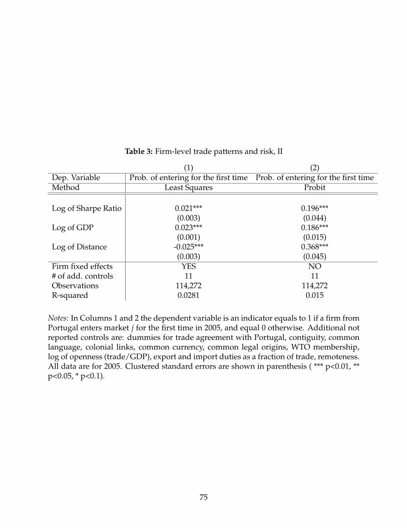
Table 3: Firm-level trade patterns and risk, II

(1) (2)Dep. Variable Prob. of entering for the first time Prob. of entering for the first timeMethod Least Squares Probit

Log of Sharpe Ratio 0.021*** 0.196***(0.003) (0.044)

Log of GDP 0.023*** 0.186***(0.001) (0.015)

Log of Distance -0.025*** 0.368***(0.003) (0.045)

Firm fixed effects YES NO# of add. controls 11 11Observations 114,272 114,272R-squared 0.0281 0.015

Notes: In Columns 1 and 2 the dependent variable is an indicator equals to 1 if a firm fromPortugal enters market j for the first time in 2005, and equal 0 otherwise. Additional notreported controls are: dummies for trade agreement with Portugal, contiguity, commonlanguage, colonial links, common currency, common legal origins, WTO membership,log of openness (trade/GDP), export and import duties as a fraction of trade, remoteness.All data are for 2005. Clustered standard errors are shown in parenthesis ( *** p<0.01, **p<0.05, * p<0.1).

75

Table 4: Aggregate trade patterns and risk

(1) (2)Dep. Variable Log of bilateral trade flows Bilateral trade flowsMethod Least Squares PPML

Log of Sharpe Ratio 0.255** 0.362***(0.093) (0.099)

Log of GDP 1.123*** 1.123***(0.032) (0.038)

Log of Distance -0.964* -0.697***(0.051) (0.065)

Source fixed effects YES YESNumber of add. controls 11 11Observations 1,225 1,225R-squared 0.9039 0.1034

Notes: In Columns 1 and 2 the dependent variable is the log of bilateral sales betweenfrom country i to j. Data is for the 35 countries in the sample, for 2005, from Comtradeand WIOD. Additional not reported controls are: dummies for bilateral trade agreement,contiguity, common language, colonial links, common currency, common legal origins,WTO membership, as well as log of openness (trade/GDP), export and import duties asa fraction of trade, remoteness of destination j. Clustered standard errors are shown inparenthesis ( *** p<0.01, ** p<0.05, * p<0.1).

76

Table 5: Firm-level trade patterns and risk, III

(1) (2) (3) (4)Dep. Variable Prob. of entering Prob. of entering Log of trade flows Log of trade flowsMethod Least Squares Least Squares Heckman Heckman

Variance -0.04*** -0.333***(0.001) (0.059)

Average covariance -0.021*** -0.14***(0.000) (0.029)

Firm fixed effects YES YES NO NONumber of controls 13 13 12 12Observations 125,346 125,346 15,369 15,369R-squared 0.125 0.125 0.11 0.12

Notes: In Columns 1-2 the dependent variable is an indicator equals to 1 if a firm from Por-tugal enters market j, and equal 0 otherwise. In Columns 3-4 the dependent variable is thelog of sales of a Portuguese firm to market j. All data are for 2005. Additional not reportedcontrols are: log of GDP, log of distance from Portugal, dummies for trade agreement withPortugal, contiguity, common language, colonial links, common currency, common legalorigins, WTO membership, log of openness (trade/GDP), export and import duties as afraction of trade, remoteness. Columns 3-4 report only the second stage of a Heckman2SLS procedure, where the excluded variable is the dummy for common language. Clus-tered standard errors are shown in parenthesis ( *** p<0.01, ** p<0.05, * p<0.1).

77

Table 6: Estimation of risk aversion

Dep. Variable Average profits

Variance of profits 0.0046***(0.0001)

Observations 1,316R-squared 0.5468

Notes: The table regresses the the average profits of Portuguese exporters on their vari-ance. Both statistics are computed using yearly data from 1995 to 2004 for firms exportingfor more than 5 years. Robust standard errors are shown in parenthesis ( *** p<0.01, **p<0.05, * p<0.1).

Table 7: Calibrated parameters

Parameter θ χ f κ0 κ1 κ2 κ3 κ4Value 5.286 0.7761 0.0075 0.683 0.187 −0.0016 −0.0630 ≈ 0

Notes: The table shows the parameters calibrated with the Simulated Method of Moments.

78

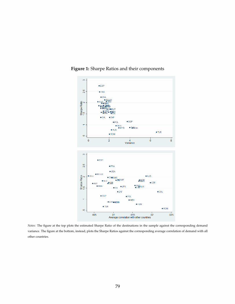
Figure 1: Sharpe Ratios and their components

Notes: The figure at the top plots the estimated Sharpe Ratio of the destinations in the sample against the corresponding demand

variance. The figure at the bottom, instead, plots the Sharpe Ratios against the corresponding average correlation of demand with all

other countries.

79

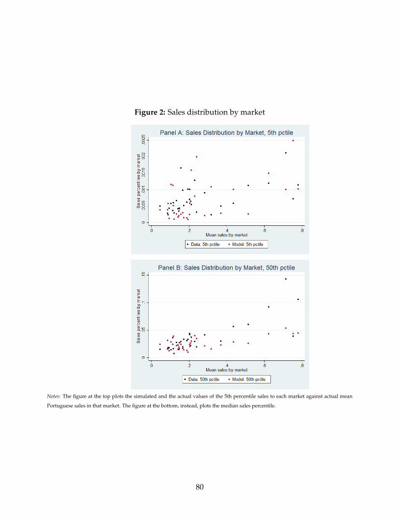
Figure 2: Sales distribution by market

Notes: The figure at the top plots the simulated and the actual values of the 5th percentile sales to each market against actual mean

Portuguese sales in that market. The figure at the bottom, instead, plots the median sales percentile.

80

Figure 3: Welfare gains from trade

Notes: The figure plots the percentage change in welfare after going to autarky. The variable on the x-axis is the Sharpe Ratio, the

country-level measure of risk-return, shown in equation (19).

Figure 4: Welfare gains from trade vs risk neutral models

Notes: The figure plots the difference between the welfare gains predicted by my model and those predicted by ACR, after moving to

autarky. The variable on the x-axis is S, the country-level measure of risk-return, shown in equation (19).

81

Figure 5: Decomposition of entrepreneurs’ welfare gains

Notes: The figure at the top plots the change in real profits after moving from autarky against the Sharpe Ratio. The figure at the

bottom, instead, plots the change in the aggregate variance of real profits against the Sharpe Ratio.

82