2010 Pulp and Paper Environmental Effects Monitoring (EEM) Technical Guidance Document

Welcome message from author
This document is posted to help you gain knowledge. Please leave a comment to let me know what you think about it! Share it to your friends and learn new things together.
Transcript

2010 Pulp and Paper Environmental Effects Monitoring (EEM) Technical Guidance Document

Pulp and Paper EEM Guidance Document Overview of EEM Program 2010
1-II
DISCLAIMER The objective of this document is to provide guidance to pulp and paper mills on how to meet the environmental effects monitoring regulatory requirements under the Pulp and Paper Effluent Regulations (PPER). This is not a legal interpretation of the PPER. For the Regulations, refer to the PPER available at http://laws.justice.gc.ca/en/F-14/SOR-92-269/index.html.
ACKNOWLEDGEMENTS The National Environmental Effects Monitoring (EEM) Office would like to thank the many people who contributed to the updating of this technical guidance document. The content was greatly improved by contributions from the members of the EEM National Team and Science Committee. The quality of the document was vastly improved through the efforts of Environment Canada’s editing team and individual members of the National EEM Office.

1
Environmental Effects Monitoring Technical Guidance Document
List of Acronyms
AETE Program: Aquatic Effects Technology Evaluation Program ANCOVA: analysis of covariance ANOVA: analysis of variance AQUAMIN: Assessment of the Aquatic Effects of Mining in Canada ASPT: average score per taxon ASTM: American Society for Testing and Materials BACI: before/after control-impact BCF: bioconcentration factor B-C Index: Bray-Curtis Index BOD: biological oxygen demand BMWP: biological monitoring working party CABIN: Canadian Aquatic Biomonitoring Network CAEAL: Canadian Association for Environmental Analytical Laboratories CALA: Canadian Association for Laboratory Accreditation CALK: combined alkaline stream CCME: Canadian Council of Ministers of the Environment CES: critical effect size C-I: control-impact C:N ratio: carbon to nitrogen ratio COV: coefficient of variation CPUE: catch per unit effort CRM: certified reference material C-SG: control–simple gradient DDW: double distilled water DIN: dissolved inorganic nitrogen D.L.: detection limit DOC: dissolved organic carbon DQOs: data quality objectives EC25: 25% effect concentration Eh: redox potential EEM: environmental effects monitoring EROD: ethoxyresorufin-O-deethylase FF: far-field FRAP: Fraser River Action Plan GC: gas chromatography MS: mass spectrometry GLP: good laboratory practice GM-IC25: geometric mean of all IC25s. GPS: global positioning system

2
GSI: gonadosomatic index HNO3: nitric acid (may want to exclude) HPLC: high-performance liquid chromatography HSB: hyper-saline brine IC25: 25% inhibition concentration ICS: invertebrate community survey ID: internal diameter IOC: investigation of cause IOS: investigation of solutions kPA: kilopascal (may want to exclude) LC50: median lethal concentration LD50: median lethal dose LCL: lower control limit LIMS: laboratory information management system LPL: lowest practical level LSI: liver somatic index LT25: time to 25% mortality LT50: time to 50% mortality LWL: lower warning limit M: molar MC-I: multiple control-impact MDL: method detection limit mean SE: mean square error MFO: mixed function oxygenase MG: multiple gradient µm: micrometre (may want to exclude) µM: micromolar (may want to exclude) MME: metal mine effluent MSE: municipal sewage effluent MSI: mantle somatic index mV: millivolts (may want to exclude) NABS: North American Benthological Society NDS: nutrient-diffusing substrate NF: near-field NHE: normal hydrogen electrode NOM: natural organic matter NRBS: Northern River Basins Study NSERC: Natural Sciences and Engineering Research Council PAH: polycyclic aromatic hydrocarbon par.: paragraph PCDD: polychlorinated dibenzo-p-dioxin PCDF: polychlorinated dibenzofuran pg/g: picograms per gram PLC: Public Liaison Committee PME: pulp mill effluent PPER: Pulp and Paper Effluent Regulations

3
PVC: polyvinyl chloride QA/QC: quality assurance / quality control RCA: reference condition approach RG: radial gradient s.: section ss.: subsection SAOB: sulphide antioxidant buffer SD: standard deviation SE: standard error SG: simple gradient SIM: selective ion monitoring SOP: standard operating procedure SPE: solid-phase extraction subpar.: sub-paragraph SRM: standard reference material SRP: soluble reactive phosphorus TCDD: tetrachlorodibenzo-p-dioxin TCDF: tetrachlorodibenzofuran TEF: toxic equivalence factor TEQ: toxic equivalent TER: toxicity emission rate TIE: toxicity identification evaluation TMP mill: thermo-mechanical pulp mill TN: total nitrogen TOC: total organic carbon TP: total phosphorus TRE: toxicity reduction evaluation TSRI: Toxic Substances Research Initiative UCL: upper control limit U.S. EPA: United States Environmental Protection Agency UWL: upper warning limit VECs: valued ecosystem components v/v: volume/volume WAWW: whole-animal wet weight WMI: Whitehorse Mining Initiative YOY: young of the year

Pulp and Paper EEM Guidance Document Overview of EEM Program 2010
1-III
TABLE OF CONTENTS
Chapter
1. OVERVIEW OF THE PULP AND PAPER ENVIRONMENTAL EFFECTS MONITORING PROGRAM
2. STUDY DESIGN, SITE CHARACTERIZATION AND GENERAL QUALITY ASSURANCE AND QUALITY CONTROL
3. EFFECTS ON FISH AND FISHERIES RESOURCES
4. EFFECTS ON FISH HABITAT: BENTHIC INVERTEBRATE COMMUNITY SURVEY
5. MEASUREMENT OF SUPPORTING ENVIRONMENTAL VARIABLES
6. SUBLETHAL TOXICITY TESTING
7. DATA ASSESSMENT AND INTERPRETATION
8. ALTERNATIVE MONITORING METHODS
9. INFORMATION MANAGEMENT AND INTERPRETIVE REPORTS
10. PUBLIC INVOLVEMENT IN PULP AND PAPER ENVIRONMENTAL EFFECTS MONITORING
11. INVESTIGATION OF CAUSE AND OF SOLUTIONS

Pulp and Paper EEM Guidance Document Overview of EEM Program 2010
1-IV
Table of Contents
1. Overview of the Pulp and Paper Environmental Effects Monitoring Program ....... 1-1 1.1 Purpose of the Guidance Document ................................................................ 1-1 1.2 The Pulp and Paper Effluent Regulations ....................................................... 1-1 1.3 Description of Environmental Effects Monitoring Studies ............................. 1-2
1.3.1 Sublethal Toxicity Testing........................................................................... 1-3 1.3.2 Biological Monitoring Studies..................................................................... 1-3
1.3.2.1 Defining and Confirming Effects......................................................... 1-3 1.3.2.2 Biological Monitoring Studies to Assess Effects ................................ 1-4
1.3.2.2.1 Fish Population Survey.................................................................... 1-5 1.3.2.2.2 Benthic Invertebrate Community Survey ........................................ 1-5 1.3.2.2.3 Fish Tissue Survey........................................................................... 1-6
1.3.2.3 Biological Monitoring Studies to Investigate Effects.......................... 1-6 1.3.2.3.1 Magnitude and Geographic Extent .................................................. 1-6 1.3.2.3.2 Investigation of Cause ..................................................................... 1-7 1.3.2.3.3 Investigation of Solutions ................................................................ 1-7
1.4 Steps in Conducting and Reporting Environmental Effects Monitoring Studies……………………………………………………………………………… 1-7
1.4.1 Submit Sublethal Toxicity Testing Results ................................................. 1-8 1.4.2 Submit Study Design ................................................................................... 1-8
1.4.2.1 Study Design for Biological Monitoring Studies to Assess Effects .... 1-8 1.4.2.2 Study Design for Investigation of Cause ............................................. 1-9 1.4.2.3 Study Design for Investigation of Solutions........................................ 1-9 1.4.2.4 Study Design for Biological Monitoring Studies to Reassess Effects. 1-9
1.4.3 Conduct Biological Monitoring Study......................................................... 1-9 1.4.4 Conduct Data Assessment............................................................................ 1-9 1.4.5 Submit Interpretive Report .......................................................................... 1-9
1.4.5.1 Interpretive Report for Biological Monitoring Studies to Assess Effects ………………………………………………………………………1-101.4.5.2 Interpretive Report for Investigation of Cause Studies ..................... 1-10 1.4.5.3 Interpretive Report for Investigation of Solutions Studies ................ 1-10
1.5 Identifying a Path through the Environmental Effects Monitoring Program 1-10 1.5.1 Critical Effect Sizes ................................................................................... 1-11 1.5.2 Magnitude of Confirmed Effects ............................................................... 1-11 1.5.3 Prioritized Effects ...................................................................................... 1-12 1.5.4 Decision Process for the Environmental Effects Monitoring Program ..... 1-13
1.5.4.1 Decision Tree 1 – For Mills with Confirmed: Effects or No Effects 1-16 1.5.4.2 Decision Tree 2 – For Mills with Unconfirmed: Effects or No Effects …………………………………………………………....…………1-18
List of Tables
Table 1-1: Fish population survey—effect indicators and endpoints .............................. 1-5 Table 1-2: Benthic invertebrate community survey—effect indicators and endpoints ... 1-6

Pulp and Paper EEM Guidance Document Overview of EEM Program 2010
1-V
Table 1-3: Critical effect sizes for pulp and paper environmental effects monitoring program.................................................................................................................. 1-11
Table 1-4: Criteria for evaluating magnitude of confirmed effects ............................... 1-11 Table 1-5: Prioritized effects ......................................................................................... 1-13
List of Figures
1-1 Decision Tree 1 – For Mills with Confirmed: Effects or No Effects……………...1-14 1-2 Decision Tree 2 – For Mills with Unconfirmed: Effects or No Effects…………...1-15

Pulp and Paper EEM Guidance Document Overview of EEM Program 2010
1-1
1. Overview of the Pulp and Paper Environmental Effects Monitoring Program
1.1 Purpose of the Guidance Document
The Pulp and Paper Effluent Regulations (PPER) under the Fisheries Act direct pulp and paper mills to conduct environmental effects monitoring (EEM) as a condition governing the authority to deposit effluent (PPER paragraph [par.] 7(1)(k)). The purpose of this document is to provide guidance on how to carry out EEM studies. For the regulatory EEM requirements, refer to sections 28 to 31 and Schedule IV.1 of the PPER located on the following website: http://laws.justice.gc.ca/eng/SOR-92-269/index.html. This guidance document replaces the 2005 version.
The recommended methodologies are based on generally accepted standards of good scientific practice and incorporate improvements based on program experience, input from multi-stakeholder working groups, consultations and external research initiatives responding to EEM needs. The current guidance also reflects the changes to EEM requirements established by the 2008 PPER amendments.
It should be emphasized that the methodologies provided in this guidance document are considered the most applicable generic designs available but are not an exhaustive list of the possible means of conducting EEM. It is assumed that each study leader has sufficient knowledge to apply these recommendations using generally accepted standards of good scientific practice and is able to determine if unique conditions exist which would warrant modification of generic study designs, while ensuring regulatory requirements are met. This first chapter provides an overview of the pulp and paper EEM program, including decision trees to assist mills in identifying the right path, based on their respective situation, through the EEM program.
Additional information and documents are available on the EEM website (www.ec.gc.ca/eem).
1.2 The Pulp and Paper Effluent Regulations
The 1992 PPER set discharge limits for total suspended solids and biochemical oxygen demand and set a requirement that all discharged effluents must be non-acutely lethal to Rainbow Trout at a 100% effluent concentration. Although the more stringent discharge limits would improve environmental protection, it was also recognized that these measures alone might not ensure adequate protection of the aquatic ecosystem at every site. In order to assess the adequacy of the effluent regulations for protecting the aquatic environment, the 1992 PPER included the requirement for an EEM program to evaluate the potential effects of effluents on fish, fish habitat and the use of fisheries resources.
In May 2004, the Regulations Amending the Pulp and Paper Effluent Regulations came

Pulp and Paper EEM Guidance Document Overview of EEM Program 2010
1-2
into force and further clarified the requirements of the 1992 PPER. Investigation of cause (IOC) studies were introduced into the EEM requirements for those mills that had observed effects of effluents.
Further amendments to the PPER came into force on August 6, 2008. These amendments improved the effectiveness and efficiency of the EEM requirements but did not change the fundamental basis of the Regulations. The major areas of change to the PPER contained in the 2008 amendments were to:
suspend EEM at mills that have ceased production for at least eight consecutive months;
streamline sublethal toxicity testing by removing the requirement to conduct the test using a fish species;
allow each component (fish or benthos) of the biological monitoring study to be assessed individually;
include an exemption from a benthic invertebrate survey based on a 1% effluent concentration in the area located within 100 metres of the point of deposit;
allow for the description of the magnitude and geographic extent of observed effects using available information, if it exists, and not necessarily requiring a separate cycle for study; and
require the investigation of solutions (IOS) that would eliminate effects.
1.3 Description of Environmental Effects Monitoring Studies EEM studies are designed to detect and measure changes in aquatic ecosystems (i.e., receiving environments). The pulp and paper EEM program is an iterative system of monitoring and interpretation phases that is used to help assess the effectiveness of environmental management measures, by evaluating the effects of effluents on fish, fish habitat and the use of fisheries resources by humans.
EEM goes beyond end-of-pipe measurement of chemicals in effluent to examine the effectiveness of environmental protection measures directly in aquatic ecosystems. Long-term effects are assessed using regular cyclical monitoring and interpretation phases designed to assess and investigate the impacts on the same parameters and locations. In this way, both a spatial characterization of potential effects and a record through time to assess changes in receiving environments are obtained.
EEM studies consist of: sublethal toxicity testing of effluent to monitor effluent quality (PPER section [s.]
29); and biological monitoring studies in the aquatic receiving environment to determine if
mill effluent is having an effect on fish, fish habitat or the use of fisheries resources (PPER s. 30).

Pulp and Paper EEM Guidance Document Overview of EEM Program 2010
1-3
1.3.1 Sublethal Toxicity Testing
Sublethal toxicity testing is conducted on effluent from the outfall structure that has potentially the most adverse environmental impact (PPER subsection [ss.] 29(1)). This testing monitors effluent quality by measuring survival, growth and/or reproduction endpoints in marine or freshwater plant and invertebrate organisms in a controlled laboratory environment. The requirement to also test a fish species was removed in the 2008 PPER amendments as results showed that the survival and growth endpoints were no longer responsive to pulp and paper mill effluents following the imposition, in 1992, of stricter discharge limits. Guidance to determine the appropriate effluent outfall to sample is found in Chapter 2. Guidance on sublethal toxicity testing is found in Chapter 6.
1.3.2 Biological Monitoring Studies
Biological monitoring studies are conducted in three- or six-year cycles. The requirements for each study are dependent on the results of the previous cycle’s results. Biological monitoring studies to assess effects are described in section 1.3.2.2 and biological monitoring studies to investigate effects are described in section 1.3.2.3. To assess effects, biological monitoring studies are conducted for three components (PPER Schedule IV.1, s. 3):
a study respecting the fish population to assess effects on fish health; a study respecting the benthic invertebrate community to assess fish habitat or
fish food; and a study respecting fish tissue dioxins and furans to assess the human usability of
the fisheries resources.
To investigate effects, biological monitoring studies are conducted for the purpose of:
describing the magnitude and geographic extent of effects; determining the causes of effects; and identifying possible solutions to eliminate effects.
The owner or operator of a mill is not required to conduct biological monitoring studies if the mill has not produced pulp or paper products for at least eight consecutive months and has not resumed production (PPER ss. 30(5)). When production of pulp or paper products resumes, biological monitoring studies are to be conducted within three years after the day on which production resumed (PPER par. 30(1)(b)).
1.3.2.1 Defining and Confirming Effects
The studies for the fish population and benthic invertebrate community components are conducted in both exposure and reference areas. The exposure area means all fish habitat and waters frequented by fish that are exposed to effluent, and the reference area means
Pulp and Paper EEM Guidance Document Overview of EEM Program 2010
1-4
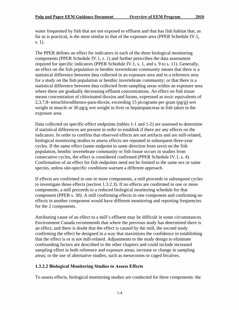
water frequented by fish that are not exposed to effluent and that has fish habitat that, as far as is practical, is the most similar to that of the exposure area (PPER Schedule IV.1, s. 1).
The PPER defines an effect for indicators in each of the three biological monitoring components (PPER Schedule IV.1, s. 1) and further prescribes the data assessment required for specific indicators (PPER Schedule IV.1, s. 1, and s. 9 to s. 11). Generally, an effect on the fish population or benthic invertebrate community means that there is a statistical difference between data collected in an exposure area and in a reference area for a study on the fish population or benthic invertebrate community; or that there is a statistical difference between data collected from sampling areas within an exposure area where there are gradually decreasing effluent concentrations. An effect on fish tissue means concentration of chlorinated dioxins and furans, expressed as toxic equivalents of 2,3,7,8- tetrachlorodibenzo-para-dioxin, exceeding 15 picograms per gram (pg/g) wet weight in muscle or 30 pg/g wet weight in liver or hepatopancreas in fish taken in the exposure area.
Data collected on specific-effect endpoints (tables 1-1 and 1-2) are assessed to determine if statistical differences are present in order to establish if there are any effects on the indicators. In order to confirm that observed effects are not artifacts and are mill-related, biological monitoring studies to assess effects are repeated in subsequent three-year cycles. If the same effect (same endpoint in same direction from zero) on the fish population, benthic invertebrate community or fish tissue occurs in studies from consecutive cycles, the effect is considered confirmed (PPER Schedule IV.1, s. 4). Confirmation of an effect for fish endpoints need not be limited to the same sex or same species, unless site-specific conditions warrant a different approach.
If effects are confirmed in one or more components, a mill proceeds in subsequent cycles to investigate those effects (section 1.3.2.3). If no effects are confirmed in one or more components, a mill proceeds to a reduced biological monitoring schedule for that component (PPER s. 30). A mill confirming effects in one component and confirming no effects in another component would have different monitoring and reporting frequencies for the 2 components.
Attributing cause of an effect to a mill’s effluent may be difficult in some circumstances. Environment Canada recommends that where the previous study has determined there is an effect, and there is doubt that the effect is caused by the mill, the second study confirming the effect be designed in a way that maximizes the confidence in establishing that the effect is or is not mill-related. Adjustments to the study design to eliminate confounding factors are described in the other chapters and could include increased sampling effort in both reference and exposure areas; increase or change in sampling areas; or the use of alternative studies, such as mesocosms or caged bivalves.
1.3.2.2 Biological Monitoring Studies to Assess Effects
To assess effects, biological monitoring studies are conducted for three components: the

Pulp and Paper EEM Guidance Document Overview of EEM Program 2010
1-5
fish population, the benthic invertebrate community and the concentration of dioxins and furans in fish tissue.
1.3.2.2.1 Fish Population Survey
A fish population survey (Chapter 3) measures indicators of fish population health in exposure and reference areas, or along an exposure gradient, to determine if mill effluent has an effect on fish. A study respecting the fish population is required if the concentration of effluent in the exposure area is greater than 1% in the area located within 250 metres of a point of deposit of the effluent in water (PPER Schedule IV.1, s. 3).
The PPER defines the fish population survey effect indicators as growth, reproduction, condition and survival (PPER Schedule IV.1, par. 11(a)(i)). The standard adult fish survey design recommends the collection of adult males and females of 2 sentinel species to determine if there are changes in the effect indicators between the exposure and reference areas, or along an effluent concentration gradient. Data collected on the effect endpoints listed in Table 1-1 are evaluated to determine if statistical differences in the effect indicators are present.
Table 1-1: Fish population survey—effect indicators and endpoints
Effect Indicators Effect Endpoints Survival Age Growth (energy use) Size-at-age (body weight to relative age) Reproduction (energy use) Relative fish gonad size (gonad weight to body weight) Condition (energy storage) Condition (body weight to length)
Relative liver size (liver weight to body weight)
The fish population survey also requires supporting water quality data to aid interpretation (PPER Schedule IV.1, s. 9). Guidance on measuring these environmental variables is presented in Chapter 5. Although the standard fish survey is recommended above other survey designs, modified methods such as a non-lethal fish survey (Chapter 3) or alternative methods (Chapter 8) may be considered under conditions where the standard survey is not effective or practical.
1.3.2.2.2 Benthic Invertebrate Community Survey

Pulp and Paper EEM Guidance Document Overview of EEM Program 2010
1-6
Mills conduct a benthic invertebrate community survey (Chapter 4) to determine if their effluent has an effect on fish habitat. A study respecting the benthic invertebrate community is conducted if the concentration of effluent in the exposure area is greater than 1% in the area located within 100 metres of a point of deposit of the effluent in water (PPER Schedule IV.1, s.3). Benthic invertebrates are collected to determine if there are changes in the effect indicators between exposure and reference areas or along an effluent concentration gradient. Data collected on the effect endpoints listed in Table 1-2 are evaluated to determine if statistical differences in the effect indicators are present.
Table 1-2: Benthic invertebrate community survey—effect indicators and endpoints
Effect Indicators Effect Endpoints Total benthic invertebrate density Number of animals per unit area Taxa richness Number of taxa Evenness index Simpson’s evenness Similarity index Bray-Curtis index
The benthic invertebrate community survey also requires supporting water- and sediment-quality data to aid interpretation (PPER Schedule IV.1, s. 9-10). Guidance on measuring these environmental variables is presented in Chapter 5. If the designs in Chapter 4 are not effective or practical, an alternative survey may be appropriate (Chapter 8).
1.3.2.2.3 Fish Tissue Survey
A fish tissue survey (Chapter 3, section 3.12) is conducted to assess if dioxins and furansaffect the use of the fisheries resources. A survey respecting the fish tissue is required if the effluent contained a measurable concentration of 2,3,7,8-TCDD or 2,3,7,8-TCDF (within the meaning of the Pulp and Paper Mill Effluent Chlorinated Dioxins and Furans Regulations pursuant to the Canadian Environmental Protection Act, 1999) since submission of the most recent interpretive report or if an effect on fish tissue was reported in the most recent interpretive report (PPER Schedule IV.1, s. 3). Fish tissue samples are collected in the exposure area from locally consumed fish or invertebrate species. Mills are also required to include in the interpretive report any complaints regarding fish flavour or odour occurring within the preceding three years (PPER Schedule IV.1, par. 12(1)(i)).
1.3.2.3 Biological Monitoring Studies to Investigate Effects
To investigate effects, mills describe the magnitude and geographical extent of effects, investigate the causes of the effects and identify the possible solutions to eliminate the effects.
1.3.2.3.1 Magnitude and Geographic Extent

Pulp and Paper EEM Guidance Document Overview of EEM Program 2010
1-7
When the 2 most recent interpretive reports indicate the same effect (same endpoint, same direction from zero) on the fish population, the benthic invertebrate community or the fish tissue, a description of the magnitude and geographic extent of the effect is required (PPER Schedule IV.1, par. 4(1)(h)). The assessment of the magnitude and geographic extent may require additional monitoring efforts to extend the sampling area further downstream or the necessary information may already exist as part of previous study results.
1.3.2.3.2 Investigation of Cause
If the most recent interpretive report indicates the magnitude and geographical extent of an effect on the fish population, benthic invertebrate community or fish tissue, or that the cause of the effect has not been identified, an IOC study is required (PPER Schedule IV.1, ss. 4(2)). The goal of an IOC study is to understand the cause of the observed effects and progress to investigate possible solutions. Guidance on IOC studies can be found in Chapter 11.
1.3.2.3.3 Investigation of Solutions
If the most recent interpretive report indicates the cause of the effect on the fish population, benthic invertebrate community or fish tissue, or that the solutions have not been identified, an IOS study is required (PPER Schedule IV.1, ss. 4(3). Guidance on IOS studies can be found in Chapter 11.
1.4 Steps in Conducting and Reporting Environmental Effects Monitoring Studies
Conducting EEM studies, as per the PPER (sublethal toxicity testing and biological monitoring studies) involves the following key steps:
Submit sublethal toxicity testing results Submit study design Conduct biological monitoring study Conduct data assessment Submit interpretive report

Pulp and Paper EEM Guidance Document Overview of EEM Program 2010
1-8
1.4.1 Submit Sublethal Toxicity Testing Results
Sublethal toxicity testing is required twice or once per calendar year depending on whether the mill deposits effluent for more or less than 120 days per year (PPER ss. 29(3)). If a mill has not produced pulp or paper products for at least eight consecutive months and has not resumed production, sublethal toxicity testing is not required (PPER ss. 29(4)).
Mills are required to submit sublethal toxicity testing results within three months after completing the tests (PPER ss. 29(2)). Test results are submitted to an Authorization Officer1 and electronic data results are submitted to Environment Canada using the submission system provided (as per PPER ss. 28(4)) on the EEM website: http://www.ec.gc.ca/esee-eem/.
1.4.2 Submit Study Design
The study design describes how the biological monitoring study will be conducted to meet the regulatory requirements (PPER Schedule IV.1, s. 4). Recommended study designs (Chapters 2, 3, 4, 8 and 11) follow recognized scientific methods and provide flexibility for site-specific conditions without subjecting field crews to unsafe sampling conditions. When more than one mill located in close proximity discharge to the same drainage basin, joint EEM studies are encouraged.
Study designs are submitted to the Authorization Officer at least six months before the commencement of sampling for biological monitoring studies. Study designs include the following:
1.4.2.1 Study Design for Biological Monitoring Studies to Assess Effects
These designs include a site characterization that describes effluent mixing in the exposure area and effluent concentrations at 100 metres and 250 metres; exposure and reference areas; anthropogenic, natural and other factors; and mill and effluent treatment processes (PPER Schedule IV.1, s. 5; guidance in Chapter 2). Also included is the scientific rationale for selecting the fish species; sampling areas; sample size; sampling periods; field and laboratory methodologies; and the methodology for determining whether the effluent has an effect on the fish population, benthic invertebrate community or fish tissue. Descriptions of the quality assurance and quality control measures that will be implemented to ensure validity of the data collected are included along with summaries of results from previous biological monitoring studies. A description of the magnitude and geographical extent of any confirmed effects, if known, is also included.
1 The Authorization Officer for each province is described in Schedule V of the PPER. Contact information for current Authorization Officers is available on the EEM website: http://www.ec.gc.ca/esee-eem/default.asp?lang=En&n=92476010-1 .

Pulp and Paper EEM Guidance Document Overview of EEM Program 2010
1-9
1.4.2.2 Study Design for Investigation of Cause
The study design includes a summary of the results of any previous biological monitoring studies that were conducted and a detailed description of the field and laboratory studies that will be used to determine the cause of the effect.
1.4.2.3 Study Design for Investigation of Solutions
The study design includes a detailed description of the studies that will be used to identify the possible solutions to eliminate the effect.
1.4.2.4 Study Design for Biological Monitoring Studies to Reassess Effects
If the most recent interpretive report indicates the solutions to eliminate the effect, or the 2 most recent interpretive reports indicated no effects, the study design includes the information described in section 1.4.2.1.
1.4.3 Conduct Biological Monitoring Study
The biological monitoring study is conducted according to the submitted study design. If circumstances arise that make it impossible to follow the study design, the owner or operator of the mill must inform the Authorization Officer without delay of the circumstances requiring deviation in the study design and of how the study will be conducted. If any deviation from study design were to occur, the mill’s environment personnel or consultants should also notify the Environment Canada regional EEM coordinator.2
1.4.4 Conduct Data Assessment
After completing the fieldwork, data assessment and interpretation are conducted to determine if mill effluent is causing an effect or effects. Data assessment and interpretation also determine the future monitoring requirements (PPER Schedule IV.1, ss. 12(1)). Specific analyses to determine if there are effects on fish, the benthic invertebrate community or fish tissue are described in Chapter 7. Data assessment for mills that have confirmed effects entails determining magnitude and geographic extent and assessing potential causes and solutions of any observed effects. Guidance on IOC and IOS studies can be found in Chapter 11.
1.4.5 Submit Interpretive Report
An interpretive report is submitted to the Authorization Officer3 within three years after the mill becomes subject to the PPER (s. 30). Subsequent interpretive reports are
2 Contact information for current regional EEM coordinators is available on the EEM website: http://www.ec.gc.ca/esee-eem/default.asp?lang=En&n=92476010-1. 3 The Authorization Officer for each province is described in Schedule V of the PPER. Contact information

Pulp and Paper EEM Guidance Document Overview of EEM Program 2010
1-10
submitted three or six years after the day on which the most recent interpretive report was required to be submitted, dependent on the results of the previous interpretive report.
Supporting data from biological monitoring studies are submitted to Environment Canada in the electronic format provided on the EEM website: http://www.ec.gc.ca/esee-eem.
The PPER outlines the information to be contained in interpretive reports for biological monitoring studies (PPER Schedule IV.1, s. 12). Chapter 9 describes interpretive reports in more detail. Brief descriptions of the different types of interpretive reports required are given below.
1.4.5.1 Interpretive Report for Biological Monitoring Studies to Assess Effects
Interpretive reports for biological monitoring studies to assess effects consist of, among other items, results of monitoring studies, raw data, results of data assessments, identification of any effects, magnitude and extent of information if available, and conclusions of the biological monitoring studies.
1.4.5.2 Interpretive Report for Investigation of Cause Studies
The IOC interpretive report consists of the cause of the effect on fish population, benthic invertebrate community or fish tissue, and any supporting raw data. If the cause was not determined, the interpretive report will also include an explanation of why it was not determined and a description of any steps that need to be taken in the next study to determine that cause.
1.4.5.3 Interpretive Report for Investigation of Solutions Studies
The IOS interpretive report consists of a description of the studies that were used to identify possible solutions to eliminate the effect and the results of those solutions. If no solutions were identified, the interpretive report will also include an explanation of the reasons why they were not identified and a description of any steps that need to be taken in the next study to identify the solutions.
1.5 Identifying a Path through the Environmental Effects Monitoring Program The EEM program involves monitoring to assess effects; monitoring to investigate observed effects (magnitude and extent, cause and solutions) and; after a period of reduced monitoring, monitoring to reassess effects. When effects in one or more components of different types and magnitudes have been observed or when the observation of effects has been inconsistent, it is recommended that mills identify the most efficient path through the EEM program. Decision trees that incorporate the
for current Authorization Officers is available on the EEM website: http://www.ec.gc.ca/esee-eem/default.asp?lang=En&n=92476010-1.

Pulp and Paper EEM Guidance Document Overview of EEM Program 2010
1-11
concepts of critical effect size (CES), prioritized effects and weight of evidence have been developed to assist mills in making this determination for the fish population and the benthic invertebrate community components.
1.5.1 Critical Effect Sizes
CESs were developed for the pulp and paper EEM program after EEM data showed that most mills observed an effect4 in at least one of the effect indicators. A CES is a threshold that indicates which effect may be of high risk. A risk-based approach was developed using CESs to identify the highest risks at this time.
The values for the fish CESs were derived from the magnitude of pulp and paper mill effluent effects, natural variability typically observed and magnitude of effects observed in Cycle 2 of the pulp and paper EEM. The values for benthic invertebrate CESs were derived from the magnitude of effects observed in Cycle 2 and what was considered exceeding the “normal range” of variability in reference areas. The CESs listed in Table 1-3 have been used since Cycle 4 (2004) with the exception of age and weight-at-age, which were added to the list in 2009.
Table 1-3: Critical effect sizes for pulp and paper environmental effects monitoring program
Fish Effect Endpoints CES Benthic Effect Endpoints CES Relative fish gonad size ± 25% Density ± 2SD Relative liver size ± 25% Richness ± 2SD Condition ± 10% Simpson’s Evenness ± 2SD Weight-at-age5 ± 25% Bray-Curtis Index > 2SD Age ± 25%Note: Differences in fish population effect endpoints are expressed as percent (%) of reference mean, while differences in benthic effect endpoints are expressed as multiples of within-reference-area standard deviations (SDs).
1.5.2 Magnitude of Confirmed Effects
The magnitude of each effect observed in the fish or benthic components can be further evaluated to determine if the magnitude of a confirmed effect is above or below the CES. The magnitude of unconfirmed effects can be approximated using a weight-of-evidence approach. Criteria were developed to assist mills in evaluating the magnitude of confirmed effects (Table 1-4).
Table 1-4: Criteria for evaluating magnitude of confirmed effects
Confirmed Effects above or equal to CES Confirmed Effects below CES
4 An effect means a statistical difference. 5 An assessment of any problems associated with aging fish needs to be conducted before an effect on weight-at-age is used to choose a path through the EEM program.

Pulp and Paper EEM Guidance Document Overview of EEM Program 2010
1-12
Same effect above or equal to CES observed in 2 most recent cycles
Same effect below CES observed in 2 most recent cycles
Same effect above or equal to CES observed in the later consecutive cycle but below CES in the earlier cycle
Same effect above or equal to CES observed in the earlier consecutive cycle but below CES in the later cycle, and there are reasons to assume effluent quality improved from the earlier to later cycle
Same effect above or equal to CES observed in the earlier consecutive cycle but below CES in the later cycle, unless there are reasons to assume effluent quality has improved from the earlier to later cycle
1.5.3 Prioritized Effects
In January 2005, the Smart Regulation Initiative Project on Improving the Effectiveness and Efficiency of Pulp and Paper Environmental Effects Monitoring was launched in response to stakeholder feedback on the EEM program. The final report and Government response to the report are available on the EEM website (www.ec.gc.ca/eem). This project brought together a group of policy experts from government, industry, and Aboriginal and environmental communities, who together made a number of recommendations for changes to the structure of the EEM program to improve its efficiency.
One of the recommendations involved strengthening the role of CESs in focusing and accelerating action toward identification of cause and solutions and in improving efficient targeting of resources by identifying mills that could reduce monitoring frequency. The report also prioritized addressing 2 nationally prevalent responses: decreases in fish gonad size and eutrophication. In addition, site-specific knowledge and conditions could lead to the designation of responses other than those prioritized by the Smart Regulation Initiative as highest risk at this time.
To achieve this recommendation, the pulp and paper CESs were reviewed to ensure their adequacy.6 Guidance was developed for using the CESs to better identify mills with effects of highest risk at this time and mills that could reduce monitoring frequency. The effects associated with a mill’s effluent are designated as highest risk when one of the prioritized effects listed in Table 1-5 has been confirmed and the magnitude of the effect was equal to or exceeded the CESs in at least one of the 2 most recent consecutive cycles.
6 Munkittrick KM, Arens CJ, Lowell RB, Kaminski GP. 2009. A review of potential methods of determining critical effects size for designing environmental monitoring programs. Environ Toxicol Chem 28(7):1361–1371.
Pulp and Paper EEM Guidance Document Overview of EEM Program 2010
1-13
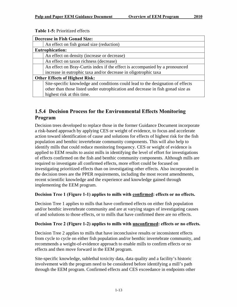
Table 1-5: Prioritized effects
Decrease in Fish Gonad Size: An effect on fish gonad size (reduction)
Eutrophication: An effect on density (increase or decrease) An effect on taxon richness (decrease) An effect on Bray-Curtis index if the effect is accompanied by a pronounced increase in eutrophic taxa and/or decrease in oligotrophic taxa
Other Effects of Highest Risk: Site-specific knowledge and conditions could lead to the designation of effects other than those listed under eutrophication and decrease in fish gonad size as highest risk at this time.
1.5.4 Decision Process for the Environmental Effects Monitoring Program Decision trees developed to replace those in the former Guidance Document incorporate a risk-based approach by applying CES or weight of evidence, to focus and accelerate action toward identification of cause and solutions for effects of highest risk for the fish population and benthic invertebrate community components. This will also help to identify mills that could reduce monitoring frequency. CES or weight of evidence is applied to EEM results to assist mills in identifying the level of effort for investigations of effects confirmed on the fish and benthic community components. Although mills are required to investigate all confirmed effects, more effort could be focused on investigating prioritized effects than on investigating other effects. Also incorporated in the decision trees are the PPER requirements, including the most recent amendments, recent scientific knowledge and the experience and knowledge gained through implementing the EEM program.
Decision Tree 1 (Figure 1-1) applies to mills with confirmed: effects or no effects.
Decision Tree 1 applies to mills that have confirmed effects on either fish population and/or benthic invertebrate community and are at varying stages of investigating causes of and solutions to those effects, or to mills that have confirmed there are no effects.
Decision Tree 2 (Figure 1-2) applies to mills with unconfirmed: effects or no effects.
Decision Tree 2 applies to mills that have inconclusive results or inconsistent effects from cycle to cycle on either fish population and/or benthic invertebrate community, and recommends a weight-of-evidence approach to enable mills to confirm effects or no effects and then move forward in the EEM program.
Site-specific knowledge, sublethal toxicity data, data quality and a facility’s historic involvement with the program need to be considered before identifying a mill’s path through the EEM program. Confirmed effects and CES exceedance in endpoints other

Pulp and Paper EEM Guidance Document Overview of EEM Program 2010
1-14
than gonad reduction, density, taxon richness and Bray-Curtis index are used as part of the site-specific evaluations and to support decisions regarding prioritization at this time.

Pulp and Paper EEM Guidance Document Overview of EEM Program 2010
1-15
Figure 1-1 DECISION TREE 1 – For mills with confirmed: effects or no effects
Have effects or no effects been confirmed?
YES
Confirmed No Effects according to 2 most recent interpretive reports (PPER s.30(3)(a), 30(4)(a))
Confirmed Effects according to 2 most recent interpretive reports (PPER Sch. IV.1 s.4(1)(h))
Are confirmed effects ≥ to CESs (Table 1-4) and prioritized (Table 1-5)?
NO
Use existing information to assess magnitude & geographic extent, describe causes and identify solutions in interpretive report
YES
Assess magnitude & geographic extent if unknown and investigate causes if unknown
Once causes are known, investigate solutions
Identify solutions in interpretive report
Submit next interpretive report in 6 years
NO See DECISION TREE 2
Note: This decision tree is designed for use with the fish population and the benthic invertebrate community components. It is designed to be used to identify a path for each of these 2 components separately. This decision tree is not designed to be used with the fish tissue component.

Pulp and Paper EEM Guidance Document Overview of EEM Program 2010
1-16
Figure 1-2 DECISION TREE 2 – For mills with unconfirmed: effects or no effects
Have effects or no effects been confirmed? See DECISION TREE 1
YES
NO
Have 2 consecutive cycles been completed?
NO
Submit next interpretive report in 3 years
YES
Use available data in a weight-of-evidence approach to interpret results and follow the appropriate path:
No interpretable results
Re-assess study design - improve/change design - use alternative study
Interpretable no effects
Interpretable small or non- prioritized effects
Use existing information to assess magnitude & geographic extent, describe causes and identify solutions in interpretive report
Interpretable large and prioritized effects (Table 1-5)
Assess magnitude & geographic extent if unknown and investigate causes if unknown
Once causes are known, investigate solutions
Identified solutions in interpretive report
Submit next interpretive report in 6 years
Note: This decision tree is designed for use with the fish population and the benthic invertebrate community components. It is designed to be used to identify a path for each of these two components separately. This decision tree is not designed to be used with the fish tissue component.

Pulp and Paper EEM Guidance Document Overview of EEM Program 2010
1-17
1.5.4.1 Decision Tree 1 – For Mills with Confirmed: Effects or No Effects Confirmed No Effects If, according to the 2 most recent interpretive reports, the studies found no effects on the fish population and/or benthic invertebrate community, the next interpretive report relating to fish and/or benthos would be required six years after the day on which the most recent interpretive report was required to be submitted.
In some cases, a mill may confirm effects in one component (fish or benthos) and confirm no effects in another component. For example, a mill in the same cycle confirms no fish effects but confirms benthos effects. In these cases, biological monitoring studies for the 2 components can be de-coupled. The next interpretive report for the component with confirmed no effects would be due six years after the day on which the most recent interpretive report was required to be submitted. The next interpretive report for all other confirmed effects would be due three years after the day on which the most recent interpretive report was required to be submitted.
Confirmed Effects If, according to the 2 most recent interpretive reports, the studies found the same effect or effects on the fish population and/or benthic invertebrate community, the mill then describes the magnitude and geographic extent of the effects, determines the cause of the effects and identifies possible solutions to eliminate the effects.
Mills are required to investigate all confirmed effects. However, for the fish and benthos components, more effort could be focused on prioritized effects of magnitudes greater than or equal to CESs than on other effects.
Prioritized Effects of Magnitudes Greater Than or Equal to CESs Mills with confirmed effects above or equal to CESs (Table 1-4) that are prioritized at this time (Table 1-5) would describe the magnitude and extent of the effects and conduct field and/or laboratory studies to determine the cause of the effects. Once the cause is known, mills would conduct studies to identify the possible solutions to eliminate the effects.
All Other Confirmed Effects Mills with confirmed effects above or equal to CESs that are not prioritized at this time, or mills with confirmed effects below the CESs, would use existing data and information to conduct all investigations, which include describing the magnitude and geographical extent of the effects, investigating the causes and identifying the solutions.
Once the most recent interpretive report has identified the solutions to eliminate all confirmed effects in a component (fish or benthos), the next interpretive report for that component would be required six years after the day on which the most recent interpretive report was required to be submitted.

Pulp and Paper EEM Guidance Document Overview of EEM Program 2010
1-18
1.5.4.2 Decision Tree 2 – For Mills with Unconfirmed: Effects or No Effects Unconfirmed Effects with No Data from Consecutive Cycles An effect is confirmed when the same effect (same endpoint, same direction from zero) is observed in 2 consecutive cycles. A mill continues to conduct biological monitoring studies in the receiving environment in a three-year cycle until at least 2 consecutive cycles of data are available. Exceptions occur when, for example, biological monitoring studies were conducted in one cycle but not the next, and resumed the following cycle. This can result in 2 sets of data that are not from consecutive cycles. If large changes in effluent quality or receiving environment conditions have not taken place, a mill may be able to use these data as if they were from consecutive cycles.
Unconfirmed Effects with Data from Consecutive Cycles Where the same effect has not been observed in 2 consecutive cycles, e.g., an endpoint showed an effect in one cycle but a different endpoint showed an effect in the next cycle, the mill could use a weight-of-evidence approach to interpret results and advance through the EEM program. Mills could re-examine and/or reanalyze the data and information from all previous EEM studies and any relevant data from other studies conducted at the same location, to conclude one of four interpretations:
No Interpretable Results Re-examination of the data does not produce an interpretable result. In this case, the mill would continue biological monitoring studies to assess effects. To improve the potential for interpretable results, the mill could redesign the study or use an alternative study.
Interpretable No Effects Re-examination of the data showed no effects based on the weight of evidence. In this case, the mill would submit the rationale to support the conclusion of no effects, including a summary of the relevant results and the reanalyzed data. The next interpretive report would be required six years after the day on which the most recent interpretive report was required to be submitted.
Interpretable Small or Non-prioritized Effects Re-examination of the data showed small effects and/or large non-prioritized effects based on the weight of evidence. An effect would be considered small if the size of the effect was not considered of highest risk at this time (similar to below CES levels). A large effect would be considered non-prioritized if it was not one of the effects listed in Table 1-5. In this case, the mill would use existing data and information to conduct all investigations, which include describing the magnitude and geographical extent of the effects, investigating the cause and identifying the solutions.
Interpretable Large and Prioritized Effects Re-examination of the data showed large, prioritized effects based on the weight of evidence. An effect would be considered large if the size of the effect was considered

Pulp and Paper EEM Guidance Document Overview of EEM Program 2010
1-19
of highest risk at this time (similar to above CES levels). In this case, the mill would describe the magnitude and extent of the effects and conduct field and/or laboratory studies to determine the cause of the effects. Once the cause of the effects is known, the mill would conduct studies to identify the possible solutions to eliminate the effects.
Once the most recent interpretive report has identified the solutions to eliminate all the effects in a component (fish or benthos), the next interpretive report for that component would be required six years after the day on which the most recent interpretive report was required to be submitted.

Pulp & Paper EEM Guidance Document Study Design, Site Characterization and General QA/QC 2010
2-I
Table of Contents
2. Study Design, Site Characterization and General Quality Assurance / Quality Control .... 2-1
2.1 Overview.......................................................................................................... 2-1
2.2 Study Design and Site Characterization .......................................................... 2-1 2.2.1 Site Characterization.................................................................................... 2-2
2.2.1.1 Plume Delineation................................................................................ 2-3 2.2.1.2 Habitat Mapping and Classification .................................................... 2-4 2.2.1.3 Aquatic Resources Inventory............................................................... 2-6 2.2.1.4 Classification Scheme for Reference Area Selection .......................... 2-6 2.2.1.5 Framework for Rivers ........................................................................ 2-10 2.2.1.6 Framework for Lakes......................................................................... 2-11 2.2.1.7 Mill History and Operations .............................................................. 2-13
2.2.2 Exposure and Reference Areas .................................................................. 2-13 2.2.2.1 Selection of Final Discharge Point for Monitoring ........................... 2-13 2.2.2.2 Selection of Exposure and Reference Areas...................................... 2-14
2.2.2.2.1 Exposure Area................................................................................ 2-14 2.2.2.2.2 Reference Area............................................................................... 2-15
2.2.3 Reporting of Field Station Positions.......................................................... 2-17 2.2.4 Modifying or Confounding Factors ........................................................... 2-17 2.2.5 Tributaries and Other Point- and Nonpoint-Source Discharges ................ 2-18 2.2.6 Natural Variation in Environmental or Habitat Conditions....................... 2-19 2.2.7 Historical Damage ..................................................................................... 2-19
2.3 General Quality Assurance / Quality Control and Standard Operating Procedures. 2-19 2.3.1 Quality Assurance and Quality Control..................................................... 2-20 2.3.2 Standard Operating Procedures ................................................................. 2-21
2.4 References...................................................................................................... 2-22
List of Tables
Table 2-1: Site characterization information for preparing an EEM study design.......... 2-3


Pulp & Paper EEM Guidance Document Study Design, Site Characterization and General QA/QC 2010
2-1
2. Study Design, Site Characterization and General Quality Assurance / Quality Control
2.1 Overview
This chapter includes information on study design, site characterization, and general quality assurance / quality control (QA/QC) information for the pulp and paper environmental effects monitoring (EEM) program. The requirements for the study design and site characterization are listed in the Pulp and Paper Effluent Regulations (PPER) (Schedule IV.1) and Chapter 1. This includes information such as timelines for EEM studies, content of study-design reports, and submission dates. Each chapter of this document contains additional information on recommended methodologies for the study design for fish, fish tissue, benthic invertebrates and alternative method studies. In addition, each chapter provides more detailed information on QA/QC.
2.2 Study Design and Site Characterization
The objective of a study design is to describe how the biological monitoring studies (a fish survey, fish tissue analysis and benthic invertebrate community survey) are to be conducted.
Study designs should describe the following (PPER, Schedule IV.1):
a summary of previous biological monitoring studies; information related to site characterization, including the results of plume
delineation studies; the objectives of the field monitoring program, including overall approach and
rationale for biological monitoring, which may be based on previous monitoring results;
statistical design criteria, hypotheses, statistical methods and data needs; a description of how the biological monitoring studies will be conducted to
determine if there are effects, taking confounding influences into consideration; field sampling plans, including what will be measured, where and when it will be
measured, location of exposure and reference sites, and rationale for selection of final discharge point;
QA/QC measures that will be taken to ensure validity of data; and schedules for field monitoring and submission of the interpretive report.

Pulp & Paper EEM Guidance Document Study Design, Site Characterization and General QA/QC 2010
2-2
2.2.1 Site Characterization
Site characterization information is submitted as part of each EEM study design (PPER Schedule IV.1, paragraph [par.] 4(a)). The requirements for site characterization are described in PPER Schedule IV.1, section (s.) 5. Table 2-1 summarizes site characterization information that should be included in the study design. For subsequent EEM studies the site characterization can be submitted in summary format, but new information (e.g., production rates) should be updated in detail. In most cases, mills will have most site characterization information available from previous assessments and historical studies. If information critical to the design of the EEM study is not available, additional field data may be required to provide adequate background for the first EEM study design, particularly with respect to hydrology and aquatic resources.
Site characterization information is used to identify suitable sampling areas that have similar habitats in the exposure and reference areas, and to obtain information on other discharges and confounding factors that may affect the interpretation of data obtained from those areas. Information on some of the unique environmental characteristics of mill sites that should be taken into consideration during the site characterization can be found in section 2.2.6.
For mills with insufficient historical information to locate reference and exposure areas, exploratory sampling may be useful. Exploratory sampling can also be used to identify habitat characteristics for effective selection of sampling stations.
An experienced field crew should be able to approximate the effluent field based on field measurements of water quality tracers (e.g., specific conductance) or preliminary dye study results, and can often identify likely depositional areas based on observed receiving water flow and circulation patterns. Thus, it is usually possible to choose some appropriate water and sediment sampling stations in the field and to complete exploratory sampling of the receiving environment concurrent with plume and depositional zone studies and critical resource/habitat inventories in a single campaign.
Much of the site characterization information can be effectively reported in map form. Maps should be of sufficient scale (e.g., 1:5000) to show the features of the study area in adequate detail. The actual scale should be reported on any map used. The geographic extent of the study area to be mapped should be determined on a site-specific basis, and should include the discharge point as well as the exposure and reference areas.

Pulp & Paper EEM Guidance Document Study Design, Site Characterization and General QA/QC 2010
2-3
Table 2-1: Site characterization information for preparing an EEM study design Information type Recommended information to be reported (where possible, some of the
information can effectively be reported in map form) General characteristics bedrock and surficial geology
topography soil and vegetation site accessibility climatology
Hydrology watershed(s) description water flow (rivers) or dispersion (lakes, estuaries, marine) characteristics general description of how effluent(s) mix(es) with receiving water bathymetry mapping (including slope in marine environments) gradient (rivers) tides (marine)—mean monthly tide height data stratification patterns (thermal and chemical) natural barriers to fish movement effluent plume delineation
Anthropogenic influences docks, wharves, ferry terminals, marinas, boat launches, public recreational zones
bridges, crossings and fordings water intakes, effluent discharges, storm water discharges, sewer overflows waste disposal sites contaminant source inventory, including point- and nonpoint sources dams, culverts, waterfalls and other barriers to fish movement surrounding land use location of aquaculture facilities
Aquatic resource characteristics
location of exposure and reference areas used in historical studies fish and shellfish species present (resident and migratory) relative abundance of fish and shellfish species use of the exposure and reference areas by fish and shellfish (spawning
grounds, nursery areas, etc.) rare, threatened or endangered fish species (if present) non-commercial fisheries (recreational and subsistence) commercial fisheries zones of macrophyte growth ecologically relevant benthic invertebrate habitat(s) and their relative
proportions, including: delineation of depositional and erosional zones substrate classification
Environmental protection systems and practices
water management effluent treatment residence time
2.2.1.1 Plume Delineation
A description of the manner in which the effluent mixes within the exposure area, including an estimate of the concentration of effluent in water at 100 metres (m) and 250 m, respectively, from each point of deposit of the effluent in water (PPER, 2008

Pulp & Paper EEM Guidance Document Study Design, Site Characterization and General QA/QC 2010
2-4
amendments, Schedule IV.1 par. 5(1)(a)), is to be described in the site characterization. If the site characterization information was submitted in a previous study design, it may be submitted in summary format, but shall include a detailed description of any changes to that information since the submission of the most recent study design (PPER Schedule IV.1, subsection [ss.] 5(2)). This description should include an indication of relative flow of the effluent and receiver, as well as seasonal variations in flow. This will give an indication of dilution rate. The description should also give an indication of the density of the effluent, and where within the water column the effluent is likely to be, prior to complete mixing. This estimate may be based on direct measurements in the field or modelling, but it is recommended that modelling be validated with field measurements.
A fish population study is conducted if the concentration of effluent is greater than 1% in the area located within 250 m of a point of deposit of the effluent in water, and a benthic invertebrate community study is conducted if the concentration of effluent in the exposure area is greater than 1% in the area located within 100 m of a point of deposit of the effluent in water (PPER Schedule IV.1, par. 3(a)(c)). If it is possible that one or both of the studies above may not need to be conducted due to the concentration of effluent being less than 1%, it is recommended that more rigorous plume delineation methods be used to document the effluent concentrations in the exposure area.
It is recommended that the description of the manner in which effluent mixes within the exposure area include the following:
identification of where in the exposure area the effluent is located, prior to mixing with the receiving water;
estimation of where in the exposure area the effluent and receiving water begin mixing, and where mixing is complete;
estimation of the effluent dilution ratio at points downstream of effluent discharge; identification of significant sources of dilution, other than the primary receiver (i.e.,
tributaries or other streams), and how the above vary with the tides and seasons.
For extensive guidance on plume delineation, please consult the Revised Technical Guidance on How to Conduct Effluent Plume Delineation Studies, available from Environment Canada (2003) at www.ec.gc.ca/esee-eem/D450E00E-61E4-4219-B27F-88B4117D19DC/PlumeDelineationEn.pdf.
2.2.1.2 Habitat Mapping and Classification
Some elements of habitat mapping and classification, as well as aquatic resource inventory, are included as part of site characterization. More detailed habitat mapping may be helpful in identifying habitat types present in the exposure and reference areas. This section provides guidance on habitat mapping and classification.

Pulp & Paper EEM Guidance Document Study Design, Site Characterization and General QA/QC 2010
2-5
The recommended method to create a habitat map is to perform a habitat classification. The recommended framework for classifying aquatic features is the classification system developed by the U.S. Fish and Wildlife Service, Classification of Wetlands and Deepwater Habitats of the United States (Cowardin et al. 1979; Busch and Sly 1992). This system allows for classification of a wide range of continental, aquatic and semi-aquatic habitats. Cowardin et al. (1979) also provides guidance on habitat description for coastal and estuarine situations.
Classification systems for marine shorelines to deep coastal areas are included in Frith et al. (1993), Booth et al. (1996), Robinson and Levings (1995), Hay et al. (1996) and Robinson et al. (1996). Specifically, estuarine classification has been reviewed by Matthews (1993), Scott and Jones (1995), Finlayson and van der Valk (1995) and Levings and Thom (1994). In the United States, the most widely used system is that of Cowardin et al. (1979) and Cowardin and Golet (1995), with expansions proposed by other authors.
The following are examples of environment-specific conditions for various habitats:
Rivers: It is recommended that river habitat descriptions include information on elevation gradient; the location of dams, falls and other barriers to fish migration; mean annual discharge and ranges; and general substrate characteristics of each river (preferably in the form of a gradient profile chart). Upstream and downstream inputs (e.g., storm water, sewer overflow, effluent from other industrial sites) should be mapped and described.
Lakes: Important habitat features of lakes include bathymetry, the locations of major inlets and outlets, and general oxygen-temperature conditions (e.g., thermal stratification, occurrences of oxygen depletion in deep water).
Open coastlines: Suggested additional mapping parameters for open coastlines (marine, Great Lakes) include depth contours, nearshore substrate characteristics, shoreline configuration, and the locations of inflowing rivers and other discharges and activities.
Estuaries: Estuaries are best described in terms of their general salinity gradients, flows, bathymetries and general substrate features. A description of tidal cycles is recommended for all marine and estuary locations. Most of the above features can be described from navigational maps, topographic maps, government publications on tides and river discharge records, and through interviews with local government officials and knowledgeable individuals.
It is recommended that bottom substrates be described. Further guidance on aquatic habitat assessment can also be found in the Department of Fisheries and Oceans and the British Columbia Ministry of the Environment and Parks (1987), Orth (1989), the Ontario Ministry of Natural Resources (1989), Plafkin et al. (1989), and the Department of Fisheries and Oceans (1990).

Pulp & Paper EEM Guidance Document Study Design, Site Characterization and General QA/QC 2010
2-6
Depositional zones in the exposure area should be identified and illustrated on the habitat map. Any information on sediment characterization (chemistry, toxicity) should be reported. Depositional zones occur where water velocity decreases, resulting in particles settling out; the finest particles settle out in the slowest current speeds. Historical contaminant or benthic invertebrate community data may be helpful in identifying sampling stations within a depositional exposure area (section 2.6). To compare resident benthic invertebrate communities, similar (but uncontaminated) sediment depositional zones should be located in the reference area. In situations where historical contamination was from a source other than the mill, two reference areas could be used: one with and one without the historically contaminated sediment.
2.2.1.3 Aquatic Resources Inventory
An aquatic resources inventory includes the identification of fish and shellfish (resident and transient) that are presently being fished commercially and non-commercially (both sport [including stocked fish] and subsistence fishing). The inventory should make particular note of fish species that may be present in sufficient numbers to be considered as a sentinel species, and of utilization (e.g., spawning, nursery) of the exposure area by fish species. In addition, any species recognized by federal, provincial or territorial authorities as rare, threatened or endangered should be included. The Committee on the Status of Endangered Wildlife in Canada website (www.cosewic.gc.ca), district fisheries biologists in federal, provincial or territorial regulatory or museum agencies, local conservation officials, and members of the local community (fishermen, Aboriginal people and public interest groups) are all sources for this type of information. Aquaculture installations should also be noted.
The potential success of field programs increases with familiarity of the study area. It is recommended that fieldwork be undertaken to verify historical information if this information is not detailed or recent.
Stocked fish are not appropriate for EEM-type monitoring, as these fish are predominantly sport fish and are not appropriate indicator species because their growth and reproduction may be altered depending on how and when they were stocked and raised. As well, stocked fish generally have no apparent reproductive success, meaning this effect indicator cannot be evaluated.
2.2.1.4 Classification Scheme for Reference Area Selection
Because reference areas will vary among different landscapes, approaches have been developed to classify land through which rivers run or in which lakes reside in order to predict aquatic biotic assemblages (Corkum 1989, 1992; Hughes 1995; Maxwell et al. 1995; Omernik 1995). A classification system is a way of simplifying sampling procedures and management strategies by organizing a variable landscape (Conquest et al. 1994). The assumption is that the classification scheme is hierarchical. The advantage of a hierarchical classification scheme is that it “offers a way to discriminate

Pulp & Paper EEM Guidance Document Study Design, Site Characterization and General QA/QC 2010
2-7
among features of the landscape at several scales of resolution” (Conquest et al. 1994). The classification scheme is based (with modifications) on one developed by the U.S. Department of Agriculture’s Forest Service (Maxwell et al. 1995). The hierarchical classification scheme is presented as a guide in the a priori selection of sampling areas. Habitat-Specific Allocation of Reference and Exposure Areas
The following specific points should be considered during the selection of reference and exposure areas and/or stations:
For Rivers: The size of the drainage basin selected is based on stream order. For example, if a
mill site is located on a second-order stream, the drainage basin area is delineated at the point the stream becomes third-order (i.e., at the junction of two second-order streams).
If there are no upstream inputs or confounding factors, the reference area(s) can be within the drainage basin and upstream of the mill.
If confounding factors, such as nonpoint- or point-source inputs, occur upstream of the effluent, the reference area(s) can be selected in nearby drainage basins with comparable habitat features (Figure 4-4).
If physical disturbance of the river valley is associated with the mill, effluent effects may be confounded by the disturbance. Accordingly, reference areas should be selected to match the physical disturbance, if possible.
The following features should be similar between reference and exposure areas: ecoregion, drainage basin area, stream order, bankfull width, channel gradient, channel pattern, habitat types, water depth, water velocity substratum composition, riparian vegetation, shoreline structure, land use, etc.
For Lakes: In lakes with a single-mill effluent and without nonpoint sources of pollution, the
sphere of influence originating from the effluent should be determined. This is particularly important for lakes in which effluent flow is not unidirectional.
If effluent plume delineation and former studies indicate that mill effects are likely to belocal and restricted, select reference areas within the lake in which the mill discharge occurs. These reference areas should occur in separate but comparable bays or basins of the lake.
If effluent plume delineation indicates that the identified effluent is dispersed throughout the lake, select reference area(s) in the nearest comparable lake within the same or adjacent drainage basin.
If nonpoint- or other point-source inputs occur elsewhere on a lake, select reference area(s) in the nearest comparable lakes within the same or adjacent drainage basin.
If the mill effluent is associated with physical disturbance in the area, effluent effects may be confounded by the disturbance. Accordingly, physically matched reference areas should be selected, if possible.
Pulp & Paper EEM Guidance Document Study Design, Site Characterization and General QA/QC 2010
2-8
The following features should be similar between reference and exposure areas: ecoregion, geological origin, drainage basin area, morphometry, slope from shoreline, habitat types, substratum composition, riparian vegetation, shoreline structure, land use, etc.
For Marine Environments: The reference area should be within the same water body and hydrographic
current or tidal regime as the exposure area. In other words, the closer the reference area is to the exposure area, the better. Benthic invertebrate communities in marine ecosystems are considerably higher in species richness, and have more complex trophic relationships, faunal size ranges and reproductive strategies, than benthic invertebrate communities in freshwater ecosystems. Because of this complexity, and the multitude of interactions between species in marine benthic invertebrates, small shifts in physical or chemical conditions can dramatically alter the overall benthic faunal community. Add to this the effect of increasing variation in chance larval settlement with increasing geographic distance (geographic “drift” in community structure) and physical barriers in complex coastlines, and it is very rare to find similar invertebrate communities from one bay or fjord to the next, and very difficult to predict specific benthic community structure based on sediment factors (for a recent review on marine invertebrate sediment interactions, see Snelgrove and Butman 1994). In order to have some confidence that the “natural” benthic community is similar enough from one coastal area to the next, there should be sufficient water exchange between them. This is more likely in open coastal areas than in isolated bays and fjords.
Reference areas, which are not in the same water body or hydrographic regime, may only be suitable for comparisons of summary characters such as shifts in abundance or species richness. If the habitat conditions are similar enough to the exposure area, it may also be possible to compare larger-scale biotic factors, such as the presence of characteristic, long-lived depth/substrate specific taxa described by Thorson (1957) as “parallel communities.”
Reference and exposure areas should have a very similar habitat type, shoreline structure (steep, mountainous, delta, marsh, etc.), bottom topography (sills, sandbars, exposure to open oceanic influences, etc.), substrate type (particle size, sorting, natural chemistry), depth properties, current regimes, physical water properties, nutrient regimes, confounding inputs and drainage characteristics.
Some special considerations are important for determining the suitability of reference areas for marine and estuarine mills. Physical factors in the estuarine/marine environment that tend to be more complex than in freshwater are salinity (including seasonal freshwater influence), tides (and tidal currents) and sediment sulphides. Other important physical factors include ice-scour or buildup, freezing, water column stagnation due to large summer freshwater runoff, re-suspension due to surface freezing in winter, dams or log booms, extraordinary siltation or clogging from logging, and periodic flooding.
In addition to the above important characteristics, the following specific points

Pulp & Paper EEM Guidance Document Study Design, Site Characterization and General QA/QC 2010
2-9
should be similar between reference and exposure areas: o intertidal areas: shoreline slope, wave exposure, light and tidal exposures,
shoreline vegetation, and encrusting fauna (although the latter may be part of the benthic taxa being monitored for a response to mill effluent)
o sub-tidal areas: seasonal water column stability and bottom oxygen depletion (stagnation).
Ecoregions
The first step in reference site selection is to use terrestrial attributes (ecoregions) with similar features. Ecoregions are defined as “part of an ecoprovince characterized by distinctive ecological responses to climate as expressed by vegetation, soils, water, and fauna” (Wiken 1986; Wickware and Rubec 1989). Ecoregion maps for Canada are available at http://ecozones.ca/english/index.html.
Drainage Basin and Geographic Scale
Catchments or drainage basins have clear hydrographic boundaries. A drainage basin is defined as the area that has a common outlet for its surface runoff. Although inter-basin transfer occurs among biota, the geoclimatic histories of large basins (1:2 000 000) are known to create barriers to dispersal through hydrographic divides and climate (Maxwell et al. 1995). It is essential to establish the geographic scale appropriate to the study design. In large-scale, synoptic surveys in which relationships are sought between landscape features and aquatic biota, the mapping scale for drainage basins is 1:250 000 (Corkum 1989, 1992, 1996; Reynoldson and Rosenberg 1996). These basins are subdivided into progressively smaller sub-basins.
Land/water interactions with respect to sediment and nutrient transport off the land and from upstream sources is integral in developing predictive models that link environmental variables and associated biota. Drainage basins may occur within ecoregions or may cross different ecoregions. Aquatic fauna are more similar to one another in drainages that occupy the same ecoregion than in drainages that occupy different ecoregions (Corkum 1992; Hughes et al. 1994).
Land Use and Vegetative Buffer Strips
Although ecoregions are defined in terms of climate and natural vegetation, natural vegetation is disturbed with human development. Land-use type is a simple measure of disturbance within the drainage basin. If there is a change in land use (e.g., land clearing for agricultural uses or logging, or fire), the biological assemblages in receiving waters will respond to those changes (Corkum 1992, 1996). Accordingly, site selection should be in drainages with comparable land use.
The degree (width and type) of a vegetated buffer strip adjacent to rivers and lakes

Pulp & Paper EEM Guidance Document Study Design, Site Characterization and General QA/QC 2010
2-10
should be recorded at all sampling areas. In reference areas where human disturbance cannot be avoided, the effect of a vegetated buffer strip moderates temperature fluctuations through shading (Budd et al. 1987), removes or reduces sediment from runoff (Young et al. 1980), and regulates nutrients and metals entering the water body (Peterjohn and Correll 1984).
2.2.1.5 Framework for Rivers
The river sampling design provides a framework for characterizing habitats at multiple scales (Meador et al. 1993). The framework for rivers is based on how they are organized in hierarchical space and how they change through time (Frissell et al. 1986). The riverine system has several hierarchical or nested levels: drainage or catchment basin, valley segment, stream reach and channel unit (Conquest et al. 1994).
Valley Segment and Stream Order
Valley segments are distinctive sections of drainage basins that possess geomorphic properties and hydrological transport characteristics that distinguish them from other segments (Cupp 1989). Montgomery and Buffington (1993) identified three valley segment types: colluvial (channelized and non-channelized), alluvial and bedrock. Valley segments can be filled with colluvium (sediment and organic matter from landslides) or alluvium (sediment transported by flow). The third valley segment has little soil and is dominated by bedrock.
Valley segments are distinguished by six criteria (Conquest et al. 1994):
1. Stream order (position in drainage network) 2. Valley slide-slope gradient 3. Ratio of valley bottom width to active channel width 4. Channel gradient 5. Stream-corridor geomorphic surface deposits 6. Channel pattern
Channel segments are assigned stream orders (Strahler 1957) for a particular map scale or aerial photograph (e.g., 1:250 000) (Newbury and Gaboury 1993).
Stream Reach
Stream reaches consist of homogeneous associations of topographic features and channel geomorphic units (Bisson and Montgomery 1996). They can be used to predict local stream response to perturbations (Montgomery and Buffington 1993). Stream reaches are useful in assessing habitat quality, aquatic productivity, fish distributions and stream health (Maxwell et al. 1995). Stream reach classification is determined using map scales of 1:12 000 to 1:24 000. Criteria used to classify stream reaches include:

Pulp & Paper EEM Guidance Document Study Design, Site Characterization and General QA/QC 2010
2-11
channel pattern channel entrenchment channel width hydraulic radius basin area channel material stream gradient bed form riparian vegetation
Simpler approaches have been adopted to identify stream reaches. For example, a straight channel has an undulating bed with alternating riffles and pools spaced at repeating intervals of 5-7 channel widths (Leopold et al. 1964; Leopold 1994). Newbury (1984) defined a stream reach to be equivalent to six times the channel width.
Channel Unit
Channel units are subdivisions of stream reaches that describe uniform microhabitats (depth and flow) and are used to identify factors that limit invertebrate and fish populations within a stream reach. Hawkins et al. (1993) proposed a three-tiered system of channel units in which the first level distinguishes riffles from pools. The second level identifies turbulent and non-turbulent riffles and distinguishes between pools formed by scour or dams. Dammed pools retain more sediment and organic debris and have more cover than scour pools. The third subdivision identifies microhabitats based on hydraulic processes and structure. Channel units are typically 10 m or less and typically cannot be mapped at a scale appropriate for land management.
Criteria for subdivision of riffles include:
gradient or water surface profile percentage of super-critical flow bed roughness mean velocity step development
Criteria for subdivision of pools include:
location (main channel or off-channel) longitudinal and cross-sectional depth profiles substrate characteristics pool-forming constraints
2.2.1.6 Framework for Lakes
The geological origin, hydrology and morphometry (obtained from maps and aerial

Pulp & Paper EEM Guidance Document Study Design, Site Characterization and General QA/QC 2010
2-12
photographs) of lakes are important in identifying sediment-water interactions and productivity of lakes (Wetzel 1975). Although thermal stratification can be predicted from morphological features, field verification is necessary. The mapping scale for lakes is typically 1:24 000 or 1:63 000 (Maxwell et al. 1995).
Origins, Location and Hydrological Linkages
Reference and exposure lakes should have the same origin, location and hydrological linkages. Lake geology ultimately affects the physical, chemical and biological characteristics of water bodies. For example, Hutchinson (1957) identifies 11 types of geomorphic processes (tectonic, volcanic, landslides, glacial activity, solution, fluviatile, wind, shorelines, organic accumulation, anthropogenic and natural dams, and meteorite impact). Surface geology and location (altitude, latitude and longitude) affect lake chemistry and thermal regimes (Winter 1977). These variables, which can be obtained from maps, are used to predict the biological composition and productivity of lakes (Dolman 1990; Winter and Woo 1990). Hydrological linkage refers to the “connection of a lake to surface or ground water” and can forecast information about lake biota (Maxwell et al. 1995). Maxwell et al. (1995) describe three types of hydrological linkages: riverine linkage (outlets and/or inlets or unconnected), groundwater linkage (gaining, losing, neutral or no recharge), and water storage regime (perennial or intermittent).
Morphometry
Lake morphometry has been used historically to predict fish yields (Ryder 1965; Kerr and Ryder 1988) and to determine species diversity (Eadie and Keast 1984; Marshall and Ryan 1987). With the exception of depth (and volume), other features can be obtained from maps. Hypsographic (cumulative depth-area or cumulative depth-volume) graphs are useful for comparing basin shapes of lakes and predicting surface area or volume for water-level control of reservoirs. Common morphological features of lakes include surface area, volume, mean and maximum depth, shoreline development, and hydraulic residence time.
Trophic State
Many lake classification systems are based on a measure of productivity (oligotrophy, mesotrophy, eutrophy). A fourth lake type (dystrophy) is used to describe lakes that receive large amounts of organic matter from external sources; these lakes are heavily stained and are known as brown-water lakes. Productivity of dystrophic lakes is low and so some limnologists group dystrophic lakes as a subclass of oligotrophic lakes. The following variables have been used to describe the trophic status of lakes:
dissolved oxygen thermal mixing (lake stratification) total phosphorus

Pulp & Paper EEM Guidance Document Study Design, Site Characterization and General QA/QC 2010
2-13
soluble reactive phosphorus total nitrogen nitrite + nitrate ammonium chlorophyll a transparency organic matter
Zone
Lakes are subdivided into an open-water pelagic zone, a shoreline or littoral zone inhabited by autotrophic vegetation, and a deeper benthic region free of vegetation (the profundal zone). The reference and exposure areas should always be located in the same zone.
2.2.1.7 Mill History and Operations
Relevant historical data regarding mill history, especially processing, effluent treatment and spills, should be reported, as they may affect interpretation of study design or results. This information is critical for identifying acceptability of historical data, and for selecting study areas. A review of historical and current mill operational data may also enable a mill operator to identify environmental concerns that can be attributed to current or past practices. To provide a better understanding of current operations, a simple schematic diagram of major sewer connections and corresponding flows of a mill could be drafted.
2.2.2 Exposure and Reference Areas
An area is qualitatively defined for sampling purposes and relates to the appropriate geographical scale encompassing one or more fundamental sampling locations (“stations”). A station is a fixed sampling location that can be recognized, re-sampled and defined quantitatively (e.g., latitude/longitude). Within EEM, the overall study area is subdivided into reference and exposure areas (for control-impact designs) or within an exposure area where there are gradually decreasing effluent concentrations (for gradient design). The PPER definition of exposure area is “all fish habitat and waters frequented by fish that are exposed to effluent,” and its definition of reference area is “water frequented by fish that is not exposed to effluent and that has fish habitat that, as far as practical, is most similar to that of the exposure area.” (PPER Schedule IV.1, s. 1).
2.2.2.1 Selection of Final Discharge Point for Monitoring
In cases where the mill has more than one final discharge point, it is recommended that sampling be done in an exposure area where the effluent has the greatest potential to have an adverse effect on the receiving environment. The mass loadings of the deleterious substance, the manner in which the effluent mixes in the exposure area, and the sensitivity of the receiving environment should all be considered when selecting which

Pulp & Paper EEM Guidance Document Study Design, Site Characterization and General QA/QC 2010
2-14
final discharge point should be used for biological monitoring.
2.2.2.2 Selection of Exposure and Reference Areas
The selection of the sampling areas is one of the most critical components of the study design and should be considered carefully to maximize the quality of the information gained from the study. The design of biological surveys is site-specific and various examples of potential study designs are presented in Chapter 4. However, this guidance is not intended to limit the mill’s flexibility to propose other potential study designs that may be suitable to the site.
2.2.2.2.1 Exposure Area
Exposure area sampling should be done in an area proximate to the effluent discharge where effects may be found. Sampling areas should ideally support both appropriate habitat for the benthic invertebrate community and populations of the selected fish species. The study design should also consider the use of the exposure area by fish species (e.g., spawning, nursery). Identification of the exposure area and its habitat features should precede the selection of reference areas, because reference areas will, as far as practicable, match the physical and chemical habitat features of the exposure area (other than the features expected to change due to the effluent).
The exposure area may extend through a number of receiving environments (e.g., different stream orders, lakes or marshes, estuarine to marine, or intertidal to sub-tidal) and contain a variety of habitat types. In most cases, the boundary of the exposure area is defined by the zone of effluent mixing. Within an exposure area, there may be near-field areas (the highest effluent exposure) and far-field areas (to determine magnitude and geographic extent). Near-field areas are outside the initial discharge zone (as described below) and have higher exposure to effluent than far-field areas. The initial discharge zone is the area where the effluent exceeds the velocity of the receiving water and the effluent is buoyant. The initial discharge zone is often characterized by visual turbulence and typically does not extend more than 5-50 m from the outfall. At least one of the near-field stations should be as near as possible to the effluent discharge point but located outside the initial discharge zone. For magnitude and geographic extent, the exposure area extends along the effluent gradient so that additional far-field areas with lower levels of effluent concentration are included. The exposure area extends geographically until a return to reference area conditions (regulatory definitions of exposure and reference areas are provided above). These far-field areas are recommended to be positioned close to the boundary of the zone of effluent mixing. Multiple sampling stations in each defined area should be used to determine spatial variation. In a gradient design, there is no reference area per se, but the response variables are evaluated along the effluent gradient.
In practical use, there will probably always be one or more far-field areas for media other than fish (e.g., water, sediment and benthos). Recommended positioning of far-field areas should be such that each area differs in regard to degree of effluent exposure. If possible, all

Pulp & Paper EEM Guidance Document Study Design, Site Characterization and General QA/QC 2010
2-15
exposure areas should be located so as to minimize or avoid exposure to non-mill discharges.
2.2.2.2.2 Reference Area
Reference areas need not represent pristine (pre-European settlement) conditions, but, rather, can comprise areas in which anthropogenic impacts, unrelated to the mill effluent, are similar to exposure areas (Simon 1991; Omernik 1995). Where feasible, the reference area should be located in the same water body as the effluent discharge, upstream of or beyond any influence from the discharge. The reference area should be suitable physically and biologically, and outside the influence of the mill or other confounding factors. When a mill is located at a headwater, and/or where no suitable reference area on the same water body is available (e.g., dams and reservoirs may be upstream), the reference area should be located in an adjacent water body with similar characteristics or a non-impacted tributary to the receiving water body. Another possibility is sampling a number of exposure areas at increasing distances from the point of discharge, representing an exposure gradient (gradient design). More than one reference area may be used, where appropriate. During magnitude and geographic extent monitoring, it may be necessary to sample more than one reference area if multiple exposure areas with different habitat types in the exposure area are sampled. As well, a more regional approach could be considered, particularly for benthic invertebrate community surveys, such as looking at several non-impacted streams (or lakes) in the area (i.e., reference condition approach).
Where historical monitoring data exist, the mill should consider using the same sampling areas from previous studies, provided they are appropriate for use in the EEM program. This will help ensure that monitoring data collected as part of the EEM program may be compared with historical data.
Baseline data (pre-effluent discharge) and multiple reference areas may assist in data interpretation. It is possible to use historical data as a baseline comparison to determine effects, but it should be treated as data additional to the mill’s data. The mill’s design should therefore include both a reference area and an exposure area (or follow a gradient design). This ensures that reference conditions have not changed and that changes observed are not incorrectly attributed to the mill, because there can be changes in parameters related to changes in environmental conditions (e.g., due to flooding or variability in annual temperatures). A reference area should be used to allow characterization of those changes that are mill-related compared to those that are not.
Where possible, sampling areas for different components (fish, benthic invertebrate community, water) should be co-located. The characteristics of the selected fish species, (e.g., mobility, habitat usage) and the different sampling gear may not always make this practical. The reference areas for benthic invertebrate sampling in some cases can be directly upstream of the exposure area, which may not be the case with fish (due to mobility). In addition, mills are encouraged to conduct benthic invertebrate community and fish monitoring studies concurrently, if justifiable biologically (e.g., if the ideal time for sampling fish reproductive parameters coincides with a suitable time for benthic

Pulp & Paper EEM Guidance Document Study Design, Site Characterization and General QA/QC 2010
2-16
community sampling; see Chapter 3 for additional information on timing for fish reproduction). Where there is more than one mill in close proximity and effluents are discharged to the same drainage basin, joint EEM studies are encouraged. Where studies are proposed jointly, sampling areas may be shared.
Environmental and biological data obtained from reference areas when compared to exposure areas detect impairment of aquatic life (Yoder 1991), diagnose stressors (Hughes et al. 1994), provide data on temporal and spatial trends (Yoder 1989) and provide data for water resource summaries for government agencies (OEPA 1990). The identification of “least impacted” areas will differ across the country. Reference areas in extremely disturbed areas may be impossible to locate. Here, studies should be designed so that reference areas with minimal degradation are located in comparable drainage basins within the same ecoregion (Hughes et al. 1994).
Usually, coastal mills do not have strictly “upstream” areas for reference sampling, because of variable directionality of current due to tidal effects. Estuarine mills may have upstream areas that are too different physically and biologically to be suitable for reference sampling. The reference area is therefore usually at least periodically downstream from the effluent discharge. Accordingly, it is important to understand the current flow patterns in the area in order to determine whether a potential reference area is “outside” mill effluent exposure.
In selecting sampling areas, the mill should take into consideration:
the location of sampling areas in previous surveys; the location of confounding influences; the size of area needed to accommodate the number of samples needed to be
collected; habitat type; site access; and other issues that could affect the mobility of fish.
In general, both sampling areas should be as follows:
As similar as possible except for exposure to effluent. Although the two areas are unlikely to be identical, it is assumed that the differences in natural characteristics (e.g., depth, substrate, flow, and water quality) will, other than mill-related factors, be small relative to the potential effect associated with the presence of effluent. If this is not the case, it should become apparent, and study design changes should be made for subsequent cycles.
Situated as closely as possible to each other (but sufficiently distant to be confident that fish from the reference area are not exposed to effluent).
Accessible, and offer safe sampling during the most appropriate season (i.e., when measurements on fish growth, reproduction, condition and survival can be taken).
Described in as much detail as possible, including the latitude and longitude as

Pulp & Paper EEM Guidance Document Study Design, Site Characterization and General QA/QC 2010
2-17
well as a written description of the area (physical, chemical and biological habitat, including measurements of temperature, depth and flow).
At a minimum, for a control/impact study, sampling should be conducted at no less than 1 reference area and 1 exposure area during the first EEM study and subsequent EEM studies (magnitude and geographic extent). The use of multiple reference areas offers the greatest statistical power to detect a meaningful difference between a reference area and exposure area (Foran and Ferenc 1999). It can also give an indication of variability among reference areas (Munkittrick et al. 2000). Differences found in the exposure area that are outside the range of values seen at a number of reference areas are more likely to be ecologically relevant (Munkittrick et al. 2000). Sampling multiple reference areas is preferred over increasing sample size (e.g., number of fish) at a single area (Environment Canada 1997).
When possible, there are advantages to selecting similar sampling areas for benthic and fish sampling so that the data can be used to help interpret responses. However, optimal benthic sampling areas may be inappropriate for the fish survey because of the characteristics of the fish species selected, the mobility of the fish, different habitat selection, and the type of sampling gear required. The sampling areas may be the same in many circumstances, but this should not be a sufficient criterion in itself for selecting the fish sampling area.
2.2.3 Reporting of Field Station Positions
The interpretive report shall contain the latitude and longitude of sampling areas in degrees, minutes and seconds; a description of the sampling areas sufficient to identify their location is required (PPER Schedule IV.1, par. 12(1)(b)). The latitude and longitude coordinates can be obtained using a variety of methods. Global positioning systems are a common tool for locating position of field stations and are recommended for this purpose. In some instances, the coordinates with stream-wise distances (e.g., river kilometres) may be useful. The recommended positioning accuracy should be determined on a site-specific basis. In some cases, where there are multiple outfalls, industrial sites may decide to collaborate on their studies.
Additional stations may be included to better represent spatial patterns in a large zone of effluent mixing, such as at a location with transects (right, mid, left), major habitats (e.g., pool and riffle), and reference / near-field / far-field sampling areas.
2.2.4 Modifying or Confounding Factors
Modifying or confounding factors can alter the interpretation of the results of biological monitoring. If the sampling areas are fairly similar, effects of modifying factors can be considered negligible. However, when there are significant differences among sampling areas, the survey design becomes confounded. In this case, it may be difficult to differentiate the effects of mill effluent from the effects of the modifying factor(s) on the response variable. For example, if the habitat type (e.g., pool) downstream of the mill was different

Pulp & Paper EEM Guidance Document Study Design, Site Characterization and General QA/QC 2010
2-18
from the habitat found upstream (e.g., riffle), the effects of habitat type on variables would confound any effects related to mill effluent. Both mill effluent and habitat type may be good predictors of any differences in variables observed upstream and downstream of the effluent discharge.
Incorporating multiple reference locations into the study design can aid in designing against spatial confounding factors, and practitioners are encouraged to do so. Design considerations for the detection of anthropogenic disturbances have been presented in the literature (see Green 1993 and references therein; Underwood 1994; Underwood 1997), and practitioners are encouraged to incorporate these considerations into their study designs.
Some examples of potential confounding factors include:
tributaries and other point- and nonpoint-source discharges (e.g., other industrial discharges, agricultural runoff, aquaculture facilities, sewage treatment plants);
natural environmental/habitat variables; and historical damage.
Attention to potential confounding factors identified during site characterization should be considered during the study design. In this way confounding factors can be minimized, or accounted for in the study design so that their influence can be assessed during data interpretation.
2.2.5 Tributaries and Other Point- and Nonpoint-Source Discharges
Tributaries provide dilution water to a main channel, lake, estuary or open ocean. This dilution water may or may not have similar chemical properties to the water body under study. Tributaries also require time and distance to mix with the main channels or receiving water body. Therefore, if there is a tributary between the reference and exposure area, the additional flow from the tributary can potentially confound the interpretation of data.
Other point- and nonpoint-source discharges may make it difficult to distinguish between effects caused by mill effluent and other discharges, particularly if they are found within close proximity to the mill effluent discharge. When other discharges are present immediately above the mill, multiple reference areas should be used. One reference area should be set between the other discharge and the effluent discharge. In this way it may be possible to account for the influence of the other discharge, and to determine the magnitude of variance in parameters due to mill effluent. If no differences between the two reference areas are found, they can be pooled to compare against the exposure area.
If there are other point-source effluent discharges not related to mills in the study area, the study design should attempt to minimize the potential effects of the confounding

Pulp & Paper EEM Guidance Document Study Design, Site Characterization and General QA/QC 2010
2-19
factors. When it is not possible to resolve the confounding factors by modifying the study design, alternative sampling designs and methods should be evaluated.
2.2.6 Natural Variation in Environmental or Habitat Conditions
Natural biological communities can differ temporally and spatially. Particularly if study areas are extensive, it is possible that natural biological communities and characteristics will be different from one location to another. It may be difficult to distinguish the influences of mill effluent, if any, relative to natural variation.
Examples of common, naturally occurring and sometimes confounding factors include:
habitat type (riffle, run, pool); substrate type (organic content, particle size); water depth; water flow rate/discharge; tidal action / currents / wave exposure; salinity; dissolved oxygen/temperature; emergent/submergent vegetation cover; water chemistry (conductivity, hardness, pH, etc.); and biological properties.
Once present in the study design, confounding effects cannot be eliminated. Only by giving careful attention to potential modifying factors identified during the pre-design phase or the previous cycles of the fish survey can the influence of modifying factors be removed or controlled in subsequent cycles. Where it is not possible to eliminate confounding factors, increasing the number of sampling areas or including additional chemical and/or biological parameters may allow the investigator to assess their influence on data interpretation.
When it is not possible to resolve the confounding factors by modifying the study design, alternative sampling designs and methods (Chapter 11) should be considered.
2.2.7 Historical Damage
When the area in which a mill releases its effluent has been subject to damage from previous activities, it may be difficult to determine differences due to current effluent-release practices. The use of an alternative method may have to be used in these situations.
2.3 General Quality Assurance / Quality Control and Standard Operating Procedures

Pulp & Paper EEM Guidance Document Study Design, Site Characterization and General QA/QC 2010
2-20
2.3.1 Quality Assurance and Quality Control
Detailed QA/QC is described in each chapter. QA/QC is a documented system incorporating adequate review, audit and internal quality control. The objective of a QA/QC program is to ensure that all field sampling and laboratory analyses produce technically sound and scientifically defensible results.
QA is a planned system of operations and procedures, the purpose of which is to provide assurance to the client that defined standards of quality are being met. Analytical QA defines the way in which tasks are to be performed in order to ensure that data meet predefined data quality goals. These tasks include not only the analysis itself but all aspects of sample handling and data management.
QA encompasses a wide range of internal and external management and technical practices designed to ensure data of known quality commensurate with the intended use of the data. External QA activities include participation in relevant inter-laboratory comparisons and audits by outside agencies. Outside audits may be based on performance in analysis of standard reference materials, or on general review of practices as indicated by documentation of sampling, analytical and QA/QC procedures, test results, and supporting data. QC is an internal aspect of QA. It includes the techniques used to measure and assess data quality and the remedial actions to be taken when data quality objectives (DQOs) are not realized. Within the context of a particular study, assurance of adequate data quality is only possible when DQOs have been defined. Users of the data should play a lead role in defining DQOs for a study and in ascertaining whether laboratory quality-control limits are consistent with these objectives.
Data quality measures should be defined in the same terms as DQOs, so that the two can be compared in project evaluation. DQOs are normally derived from intended data uses (e.g., hypotheses to be tested, summary statistics involved, and total uncertainty that can be tolerated). Total uncertainty includes imprecision (sampling, analytical, environmental) plus any analytical bias that may occur (Taylor 1987). Objectives can be established for each component and for total uncertainty, and should be incorporated into the QA project plans. The various components of imprecision can be estimated using field replicate data and laboratory replicate data.
QA functions, the personnel responsible for each QA function, and corrective actions when performance limits are exceeded should be identified in the quality management plan.
QC activities define the boundaries of acceptable performance for the measurement system, and include the routine checks (data quality measures) that indicate whether the system is performing to specification. Data reporting generally stops and corrective actions are initiated when the system goes out of control. Range and average-control charting methods have been described elsewhere (OMOE 1984; ASTM 1985, 1986; Dux 1986).
An outline of recommended QA/QC requirements for specific components of the fish survey

Pulp & Paper EEM Guidance Document Study Design, Site Characterization and General QA/QC 2010
2-21
(Chapter 3), benthic invertebrate survey (Chapter 4), effluent and water quality analysis (Chapter 5), and sediment quality analysis (Chapter 5) are presented in each respective chapter. This information focuses on QC in the field, laboratory, data analysis, and reporting.
2.3.2 Standard Operating Procedures
Standard operating procedures (SOPs) are fundamental to any QA/QC program. All field and lab procedures should be conducted according to SOPs in order to ensure quality control. SOPs should describe the following in detail:
the field programs’ requirements for sampling methods and procedures, sample handling, labelling, equipment, preserving, record keeping, and shipping; and
the analytical methods and procedures, sample handling, labelling, equipment, test system implementation, record keeping and so forth of all laboratory analyses.
Each SOP should be a written, detailed method accessible to each analyst. SOPs should be based on procedures developed by a standard-setting organization such as Environment Canada, the U.S. Environmental Protection Agency, the American Society for Testing and Materials, or the American Public Health Association. Where methods are not well validated, it is recommended that the SOP be thoroughly referenced to the relevant literature and contain all the elements outlined in CALA (1991). In-house validation of data should be appended to the SOP and contain the QA/QC procedures, including the types and frequencies of QC samples to be analyzed, the expected levels of precision, accuracy and recovery, and the method detection limits.
While chemical analysis procedures tend to be reasonably well documented, sampling procedures in general, and sampling design in particular, are often overlooked. Sampling error is usually a large component and often the dominant component of uncertainty in environmental measurements. SOPs that include field operations will help to reduce this uncertainty or at least ensure that it is quantified. All field staff should be familiar with the SOPs for any field survey work.
Emphasis should be placed on measures to prevent inadvertent contamination of samples and to ensure sample integrity. In addition, SOPs should specify the proper preparation of all sampling gear and supplies, and the proper calibration of all instrumentation (such as meters).

Pulp & Paper EEM Guidance Document Study Design, Site Characterization and General QA/QC 2010
2-22
2.4 References [ASTM] American Society for Testing and Materials. 1985. Standard practice for establishing conditions for laboratory sensory evaluation of foods and beverages. Philadelphia (PA): American Society for Testing and Materials. ASTM E480-84.
[ASTM] American Society for Testing and Materials. 1986. Physical requirement guidelines for sensory evaluation laboratories. Philadelphia (PA): American Society for Testing and Materials. ASTM STP 913.
Bisson PA, Montgomery DR. 1996. Valley segments, stream reaches, and channel units. In Hauer FR, Lamberti GA, editors. Methods in stream ecology. San Diego (CA): Academic Press. p. 23-52.
Booth J, Hay D, Truscott J. 1996. Standard methods for sampling resources and habitats in coastal subtidal regions of British Columbia: Part I - Review of mapping with preliminary recommendations. (Canadian Technical Report of Fish and Aquatic Sciences. 2118). Nanaimo (BC): Fisheries and Oceans Canada. 53pp.
Budd WW, Cohen PL, Saunders PR, Steiner FR. 1987. Stream corridor management in the Pacific Northwest: 1. Determination of stream-corridor widths. Environ Manag 11:587-597.
Busc, W-DN, Sly PG, editors. 1992. The development of an aquatic habitat classification system for lakes. Boca Raton (FL): CRC Press. 225 p.
[CALA] Canadian Association for Laboratory Accreditation (formerly [CAEAL] Canadian Association of Environmental Analytical Laboratories). 1991. Code of practice and QA manual for laboratory analysis of sewage treatment effluent in support of the MISA Program. Draft report prepared for CAEAL and the Ontario Ministry of the Environment by Zenon Environmental Laboratories.
Conquest LL, Ralph SC, Naiman RJ. 1994. Implementation of large-scale stream monitoring efforts: sampling design and data analysis issues.. In Loeb SL, Spacie A, editors. Biological monitoring of aquatic systems. Boca Raton (FL): Lewis Publ. p. 69-90.
Corkum LD. 1989. Patterns of benthic invertebrate assemblages in rivers of northwestern North America. Freshwat Biol 21:191-205.
Corkum LD. 1992. Spatial distributional patterns of macroinvertebrates along rivers within and among biomes. Hydrobiologia 239:101-114.
Corkum LD. 1996. Responses of chlorophyll a, organic matter and macroinvertebrates to

Pulp & Paper EEM Guidance Document Study Design, Site Characterization and General QA/QC 2010
2-23
nutrient additions in rivers flowing through agricultural and forested land. Arch Hydrobiol 136:391-411.
Cowardin LM, Carter V, Golet FC, LaRoe ET. 1979. Classification of wetlands and deepwater habitats of the United States. Washingtin (DC): U.S. Fish and Wildlife Service. FWS/OBS-79/31.
Cowardin LM, Golet CF. 1995. US Fish and Wildlife Service 1979 wetland classification: a review. Vegetatio 118:139-152.
Cupp CE. 1989. Valley segment type classification for forested lands of Washington. Timber, Fish & Wildlife AM-89-001. Olympia (WA): Washington Forest Protection Association. 42 pp.
Department of Fisheries and Oceans. 1990. Coastal/estuarine habitat description and assessment manual. Part II. Habitat description procedures. Coquitlam (BC): prepared by G.L. Williams and Associates Ltd.
Department of Fisheries and Oceans and British Columbia Ministry of the Environment and Parks. 1987. Fish Habitat Inventory and Information Program: Stream Survey Field Guide. Vicortia (BC): Resources Inventory Committee.
Dolman WB. 1990. Classification of Texas reservoirs in relation to limnology and fish community associations. Trans Am Fish Soc 119:511-520.
Dux JP. 1986. Handbook of quality assurance for analytical chemistry laboratory. New York (NY): Van Nostrand Reinhold Co.
Eadie JM, Keast A. 1984. Resource heterogeneity and fish species diversity in lakes. Can J Zool 62:1689-1695.
Environment Canada. 1997. Fish Survey Expert Working Group report. EEM/1997/6. Ottawa (ON): Environment Canada.
Environment Canada. 2003. Revised technical guidance on how to conduct effluent plume delineation studies. Available from www.ec.gc.ca/esee-eem/D450E00E-61E4-4219-B27F-88B4117D19DC/PlumeDelineationEn.pdf
Finlayson CM, van der Valk AG. 1995. Wetland classification and inventory: a summary. Vegetatio 118(1-2):185-192.
Ferenc SA, Foran JA. Eds. 1999. Multiple stressors in ecological risk and impact assessment. Pensacola (FL): SETAC Press.
Frissell CA, Liss WL, Warren CE, Hurley MD. 1986. A hierarchical framework for stream habitat classification: viewing streams in a watershed context. Environ Manag 10:199-214.

Pulp & Paper EEM Guidance Document Study Design, Site Characterization and General QA/QC 2010
2-24
Frith HR, Seraring G, Wainwright P, Harper H, Emmett B. 1993. Review of habitat classification systems and an assessment of their suitability to coastal B.C. Unpublished report. Prepared for Environmental Emergency Services Branch, Environment Canada by L.G.L. Ltd., Sidney (BC)
Green RH. 1993. Application of repeated measures designs in environmental impact and monitoring studies. Australian J Ecol 18:81-98.
Hay DE, Waters RD, Boxwell TA, editors. 1996. Proceedings marine ecosystem monitoring network workshop, Nanaimo, B.C. March 28-30. 1995. (Canadian Technical Report of Fish and Aquatic Sciences 2108). Nanaimo (BC): Fisheries and Oceans Canada.160 p.
Hawkins CP, Kershner JL, Bisson PA, Bryant MD, Decker LM, Gregory SV, McCullough DA, Overton CK, Reeves GH, et al. 1993. A hierarchical approach to classifying stream habitat features. Fisheries 18:3-12.
Hughes RM. 1995. Defining acceptable biological status by comparing with reference conditions. In Davis WS, Simon TP, editors. Biological assessment and criteria: tools for water resource planning and decision making. Boca Raton (FL): Lewis Publishers. p. 31-47.
Hughes RM, Heiskary SA, Matthews WJ, Yoder CO. 1994. Use of ecoregions in biological monitoring. In Loeb SL, Spacie A, editors. Biological monitoring of aquatic systems. Boca Raton (FL): Lewis Publishers. p. 125-149.
Hutchinson GE. 1957. A treatise on limnology. Vol I. Geology, physics, and chemistry. New York (NY): John Wiley & Sons Inc. 1015 p.
Kerr SR, Ryder RA. 1988. The applicability of fish yield indices in freshwater and marine ecosystems. Limnol Oceanogr 33:973-981.
Leopold LB. 1994. A view of the river. Cambridge (MA): Harvard University Press. 297 p.
Leopold LB, Wolman GM, Miller JP. 1964. Fluvial processes in geomorphology. San Francisco (CA): W.H. Freeman & Co. 522 p.
Levings CD, Thom RM. 1994. Habitat changes in the Georgia Basin: implications for resource management and restoration. In Wilson RCH, Beamish RJ, Aitkens F, Bell, J, editors. Review of the marine environment and biota of Strait of Georgia, Puget Sound and Juan de Fuca Strait: Proceedings of the BC/Washington Symposium on the Marine Environment Jan 13,14 1994. (Canadian Technical Report of Fish and Aquatic Sciences 1948). Ottawa (ON): Fisheries and Oceans Canada. p. 330-351.
Marshall TR, Ryan PA. 1987. Abundance and community attributes of fishes relative to environmental gradients. Can J Fish Aquat Sci 44:196-215.

Pulp & Paper EEM Guidance Document Study Design, Site Characterization and General QA/QC 2010
2-25
Matthews GWT. 1993. The Ramsar Convention; its history and development. Glan (CH): Ramsar Caonvention Bureau.
Maxwell JR, Edwards CJ, Jensen ME, Paustian SJ, Parrott H, Hill DM. 1995. A hierarchical framework of aquatic ecological units in North America (Nearctic Zone). Gen. Tech. Rep. NC-176. St. Paul (MN): U.S. Department of Agriculture, Forest Service, North Central Forest Experimental Station. 72 p.
Meador MR, Hupp CR, Cuffney TF, Gurtz ME. 1993. Methods for characterizing stream habitat as part of the national water-quality assessment program. Raleigh (NC): U.S. Geological Survey. Open-File Report 93-408.
Montgomery DR, Buffington JM. 1993. Channel classification, prediction of channel response, and assessment of channel condition. Washington State Timber/Fish/Wildlife Agreement. Report TFW-SH10-93-002. Olympia (WA): Department of Natural Resources.
Munkittrick KR, McMaster M, Van Der Kraak G, Portt C, Gibbons W, Farwell A, Gray M. 2000. Development of methods for effects-based cumulative effects assessment using fish populations: Moose River Project. Pensacola (FL): SETAC Press. xviii + 236 p.
Newbury RW. 1984. Hydrological determinants of aquatic insect habitats. In Resh VH, Rosenberg DM, editors. The ecology of aquatic insects. New York (NY): Praeger. p. 323-357.
Newbury RW, Gaboury MN. 1993. Stream analysis and fish habitat design. A field manual. Gibsons (BC): Newbury Hydraulics Ltd., The Manitoba Habitat Heritage Corporation, Manitoba Fisheries Branch.
[OEPA] Ohio Environmental Protection Agency. 1990. Ohio Water Resource Inventory. Columbus (OH): Ohio Environmental Protection Agency.
Omernik JM. 1995. Ecoregions: a spatial framework for environmental management. In Davis WS, Simon TP, editors Biological assessment and criteria. Tools for water resource planning and decision making. Boca Raton (FL): Lewis Publishers. p. 49-62
Ontario Ministry of Natural Resources. 1989. Manual of instructions. Aquatic habitat inventory surveys. Toronto (ON): Ontario Ministry of Natural Resources.
[OMOE] Ontario Ministry of the Environment. 1984. Principles of Control Charting. King DE, Ronan RC, editors. Laboratory Services Branch, Data Quality Report Series. Rexdale (ON): Ontario Ministry of the Environment.
Orth DJ. 1989. Aquatic habitat measurements. In Neilson LA, Johnson DL, editors. Fisheries techniques. Bethesda (MD): Am. Fish. Soc. p. 61-84

Pulp & Paper EEM Guidance Document Study Design, Site Characterization and General QA/QC 2010
2-26
Peterjohn WT, Correll DL. 1984. Nutrient dynamics in an agricultural watershed: observation on the role of a riparian forest. Ecology 65:1466-1475.
Plafkin JL, Barbour MT Porter KD Gross SK, Hughs RM. 1989. Rapid bioassessment protocols for use in streams and rivers: benthic macroinvertebrates and fish. Washington (DC): U.S. Environmental Protection Agency. EPA/444/4-89-001.
Reynoldson TD, Rosenberg DM. 1996. Sampling strategies and practical considerations in building reference data bases for the prediction of invertebrate community structure.. In Bailey RC, Norris RH, Reynoldson TB, editors. Study design and data analysis in benthic macroinvertebrate assessments of freshwater ecosystems using a reference site approach. Technical Information Workshop North American Benthological Society, 44th Annual Meeting, Kalispell, Montana. p. 1-31.
Robinson CLK, Levings C.D. 1995. An overview of habitat classification systems, ecological models and geographic information systems applied to shallow foreshore marine habitats. (Canadian Manuscript Report of Fish and Aquatic Sciences 2322). West Vancouver (BC): Fisheries and Oceans Canada. 65 p.
Robinson CLK, Hay DE, Booth J, Truscott J. 1996. Standard methods for sampling resources and habitats in coastal subtidal regions of British Columbia: Part 2 - Review of sampling with preliminary recommendations. (Canadian Technical Report of Fish and Aquatic Sciences 2119). Nanaimo (BC): Fisheries and Ocean Canada. 119 p.
Ryder RA. 1965. A method for estimating the potential fish production of north temperate lakes. Trans Am Fish Soc 94:214-218.
Scott DA, Jones TA. 1995. Classification and inventory of wetlands. Vegetatio 118:1-16.
Simon TP. 1991. Development of biotic integrity expectations for the ecoregions of Indiana. I. Central Corn Belt Plain. Chicago (IL}: U.S. Environmental Protection Agency, Region V, Environmental Sciences Division, Monitoring and Quality Assurance Branch, Ambient Monitoring Section. EPA 905/9-91/025.
Snelgrove RVR, Butman CA. 1994. Animal sediment relationships revisited: cause versus effect. Oceanog Mar Biol Ann Rev 32:111-178.
Strahler AN. 1957. Quantitative analysis of watershed geomorphology. Am Geophys Union Trans. 38:913-920.
Taylor JK. 1987. Quality assurance of chemical measurements. Chelsea (MI): Lewis Publishers Inc.
Thorson G. 1957. Bottom communities(sublitorral or shallow shelf). In Hedgepeth JW, editor. Treatise on marine ecology and paleoecology. Vol 1.Memoirs of the Geological Society of America 67. p. 461-534.

Pulp & Paper EEM Guidance Document Study Design, Site Characterization and General QA/QC 2010
2-27
Underwood AJ. 1994. On beyond BACI: sampling designs that might reliably detect environmental disturbances. Ecol Appl 4(1):3-15.
Underwood AJ. 1997. Experiments in ecology: their logical design and interpretation using analysis of variance. Cambridge (UK): Cambridge University Press. 504 p.
Wetzel RG. 1975. Limnology. Philadelphia (PA):W.B. Saunders Co. 743 p.
Wickware GM, Rubec CDA. 1989. Ecoregions of Ontario. (Ecological Land Classification Series 26). Ottawa (ON): Environment Canada. 37 p.
Wiken E. 1986. Terrestrial ecotones of Canada. (Ecological Land Classification Series 19). Ottawa (ON):Environment Canada.
Winter WT. 1977. Classification of hydrological settings of lakes in the north-central United States. Wat Resources Res 134:753-767.
Winter WT, Woo MK. 1990. Hydrology or lakes and wetlands. In Wolman MG, Riggs HC, editors. Surface water hydrology. Boulder (CO): The Geological Society of America. p. 159-187.
Yoder CO. 1989. The development and use of biological criteria for Ohio surface waters. In Water quality standards for the 21st century. Washington (DC): Office of Water, U.S. Environmental Protection Agency., p. 139-146.
Yoder CO. 1991. Answering some concerns about biological criteria based on experiences in Ohio. In Water quality standards for the 21st century. Washington (DC): Office of Water, U.S. Environmental Protection Agency. p. 95-104.
Young RA, Huntrods T, Anderson W. 1980. Effectiveness of vegetated buffer strips in controlling pollution from feedlot runoff. J Environ Qual 9:483-497.

Pulp and Paper EEM Guidance Document Effects on Fish and Fisheries Resources 2010
3-I
Table of Contents
3. Effects on Fish and Fisheries Resources.................................................................. 3-1
3.1 Overview.......................................................................................................... 3-1
3.2 Study Design Considerations........................................................................... 3-1 3.2.1 Selection of Reference and Exposure Areas................................................ 3-2
3.2.1.1 Sampling of Exposure and Reference Areas ....................................... 3-3 3.2.1.2 Adequacy of the Reference Area ......................................................... 3-4
3.2.2 Confounding Factors.................................................................................... 3-4 3.2.3 Marine Discharges ....................................................................................... 3-4
3.3 Selection of Sentinel Fish Species ................................................................... 3-5 3.3.1 Community Survey ...................................................................................... 3-7 3.3.2 Immature Fish .............................................................................................. 3-7 3.3.3 Small-bodied Fish Species........................................................................... 3-8 3.3.4 Live-bearers ................................................................................................. 3-9
3.4 Effect Indicators............................................................................................... 3-9 3.4.1 Lethal Sampling ......................................................................................... 3-10
3.4.1.1 Survival .............................................................................................. 3-12 3.4.1.2 Energy Use (Growth and Reproduction) ........................................... 3-13 3.4.1.3 Energy Storage (Condition) ............................................................... 3-14 3.4.1.4 Abnormalities..................................................................................... 3-14
3.4.2 Non-lethal Sampling .................................................................................. 3-15 3.4.2.1 Survival (Size Distributions) ............................................................. 3-17 3.4.2.2 Energy Use......................................................................................... 3-17 3.4.2.3 Condition ........................................................................................... 3-18
3.4.3 Wild Molluscs............................................................................................ 3-18
3.5 Timing of Sampling ....................................................................................... 3-19
3.6 Verification of Fish Exposure........................................................................ 3-23
3.7 Power Analysis .............................................................................................. 3-25 3.7.1 Power and Significance Level ................................................................... 3-25 3.7.2 Effect-Size.................................................................................................. 3-25
3.8 Fish Sampling Methods ................................................................................. 3-26 3.8.1 Bycatch ...................................................................................................... 3-27 3.8.2 Remote Sensing ......................................................................................... 3-27 3.8.3 Alternative Methods .................................................................................. 3-27
3.9 Fish Survey Quality Assurance and Quality Control..................................... 3-28 3.9.1 Field Practices to Improve Data Analysis and Interpretation .................... 3-28 3.9.2 Quality Control in the Field ....................................................................... 3-28 3.9.3 Determination of Sampling Effort ............................................................. 3-29

Pulp and Paper EEM Guidance Document Effects on Fish and Fisheries Resources 2010
3-II
3.9.3.1 Examples of Calculations of Sampling Effort ................................... 3-30 3.9.4 Consultation with Regional EEM Coordinators and Implementation in the Field 3-32 3.9.5 Data Entry .................................................................................................. 3-33 3.9.6 Quality Control in the Laboratory ............................................................. 3-33
3.10 Data Analysis ................................................................................................. 3-34 3.10.1 Statistical Analysis................................................................................. 3-34
3.11 Fish Tissue Analysis for Dioxins and Furans ................................................ 3-35 3.11.1 Tissue Sample Collection and Preparation ............................................ 3-36 3.11.2 QA/QC Criteria for Chlorinated Dioxins and Furans Analyses ............ 3-36
3.12 References...................................................................................................... 3-38
List of Tables
Table 3-1: Required fish survey measurements, expected precision and summary statistics.................................................................................................................. 3-11
Table 3-2: Suggested aging structures for Canadian fish species.................................. 3-13 Table 3-3: Fish survey effect indicators and endpoints for various study designs........ 3-15 Table 3-4: Generalizations and suggested optimal sampling times for fish species in EEM
................................................................................................................................ 3-20 Table 3-5: Fish species commonly used in EEM, aspects to consider during study design,
and recommended sampling times (based on Barrett and Munkittrick, 2010) ...... 3-21

Pulp and Paper EEM Guidance Document Effects on Fish and Fisheries Resources 2010
3-1
3. Effects on Fish and Fisheries Resources
3.1 Overview
Fish monitoring for the environmental effects monitoring (EEM) program may consist of a fish population survey and tissue analyses to determine if the mill effluent is having an effect on fish and fisheries resources. Detailed requirements and timelines are found in Chapter 1 and in the Pulp and Paper Effluent Regulations (PPER) (SOR/2008-239).
For the purposes of EEM, fish includes shellfish, crustaceans and marine animals, as per section 2 of the Fisheries Act, but excludes parts of these organisms (PPER Schedule IV. 1, section (s.) 1).
The fish survey provides an assessment of whether there are differences in the growth, reproduction, condition and survival of the fish population between exposed and reference areas or within an exposure area along a gradient of effluent concentrations. Note that a mill is required to conduct a study of the fish population if the concentration of effluent in the exposure area is greater than 1% in the area located within 250 metres (m) of a point of discharge of the effluent in water (PPER Schedule IV.1, paragraph [par.] 3(a)).
In addition to the fish survey, biological monitoring studies may also include a study respecting fish tissue levels of chlorinated dioxin and furan congeners in edible portions of fish. A study respecting fish tissue is conducted if, since the submission of the most recent interpretive report, the effluent contained a measurable concentration of 2,3,7,8-TCDD (tetrachlorodibenzo-p-dioxin) or 2,3,7,8-TCDF (tetrachlorodibenzofuran), or if an effect on fish tissue was reported in the most recent interpretive report (PPER Schedule IV.1, par. 3(b)).
A tainting evaluation may also be conducted to assess the usability of the fisheries resources by determining if any fish contains an abnormal odour or flavour as a result of the discharge of pulp and paper effluents. A tainting evaluation may be recommended following a complaint or if a previous sensory evaluation demonstrated that tainting was an issue. Consult the Authorization Officer for more information on tainting evaluation, if such a survey is necessary.
3.2 Study Design Considerations
General information regarding study designs is discussed in Chapter 2. The study design requirements and the definitions of effect for the fish population survey and fish tissue survey are discussed in Chapter 1.
To evaluate the effect of effluent on fish, the following questions should be answered:

Pulp and Paper EEM Guidance Document Effects on Fish and Fisheries Resources 2010
3-2
Is there an effect? Is the effect mill-related? Is the magnitude and extent of the effect known? Is the mill-related cause of the effect known?
Each mill’s EEM representatives or consultants should consult with the regional EEM authority to review the results of the previous cycle’s site selection, species selection, fishing effort, etc., and to discuss the selection of the most appropriate options for the current cycle. The results of previous cycles, historical data, and local knowledge should be used to assess:
the suitability and capture success of selected sentinel species the adequacy of the reference area the appropriateness of sampling methods and required equipment.
Mills may want to make changes between cycles, including increasing sampling effort; changing sampling methods, equipment or fish species; selecting different exposure or reference areas; or using alternative monitoring techniques. Changes in the study design may need to be made for various reasons, including the following:
The results indicate that power was insufficient in the previous cycle due to collection of a low number of fish or high variability.
The species characteristics were not measurable, not suitable, or there are concerns about the status of fish populations.
It is uncertain if the fish were exposed to effluent. Reference sites were inappropriate.
Concerns raised about EEM studies (and field studies in general) can be separated into concerns about the adequacy of the reference sites, the potential impacts of confounding factors (e.g., potential influences of genetics on the variability of species characteristics), the ecological relevance of effect indicators used, the influences of natural variability, and concerns over statistical design issues. This guidance will attempt to provide input to deal with these issues.
3.2.1 Selection of Reference and Exposure Areas
The two main study designs are control-impact and gradient designs. The choice of reference area is the number one problem with control-impact field studies (Munkittrick et al. 2009). Ideally, a reference site would be located upstream, in similar habitat, and free of confounding influences, with a natural barrier that limits movement between sites. This situation is seldom available. The main issues cited regarding reference areas include whether the reference site is (a) comparable in terms of habitat; (b) free from the issue of concern (i.e., exposure), and from confounding influences (further discussed in Chapter 2); (c) open to movement of fish from the exposure area (fish in an upstream reference area could have been exposed previously; fish in the exposure area could be
Pulp and Paper EEM Guidance Document Effects on Fish and Fisheries Resources 2010
3-3
transient, reducing exposure to potential effects); and (d) whether the exposed fish were exposed to the effluent or stressor of interest.
No reference site is perfect. The ideal situation involves having data from before construction or initiation of the stressor of interest (e.g., before/after control-impact [BACI] design; outlined further in Chapter 4). Study sites that have barriers that prevent fish from moving between sites (e.g., dams, waterfalls, beaver dams) may be a good alternative, providing that the barrier does not alter the habitat. In open-water areas, choosing a species that has limited mobility improves the confidence that fish are not moving, but increases the potential influences of local differences in habitat. One difficult situation to interpret arises when there are no statistical differences in fish measurements between the areas, and there are no barriers restricting movement. In these cases, an indicator of exposure to the effluent is recommended, which can be chemical or physiological (e.g., liver enzyme induction, stable isotope signatures [Galloway et al. 2003; Dubé et al. 2006]).
If there are significant differences in fish characteristics between reference and exposure areas, there can be high confidence that fish are not moving between sites. Although differences are seen, variability in fish parameters (e.g., growth, weight, condition) is a function of a number of factors, not all of which will be related to the discharge of effluent. The selection of appropriate fish species for monitoring, survey timing and sampling gear will also facilitate the interpretation of any differences detected. Nevertheless, other natural and anthropogenic factors may influence effects on the fish and fish tissue and confound interpretation of the data. The requirement to confirm effects was developed to increase the confidence, over two cycles, that effects are mill-related.
3.2.1.1 Sampling of Exposure and Reference Areas
The exposure area should be selected to ensure that the fish collected have been exposed to the effluent. It should be sampled first to determine which fish species are present, and their relative abundance within the area. The reference area can then be selected to provide fish of the same species that are available at the exposed site. Timing of sampling should be as close as possible between sites, to minimize temporal variability. The choice of time period for sampling will depend on factors such as time of year, stage of reproductive development, and potential habitat differences between sites (water temperature differences, etc.), but it is recommended that, if possible, all sampling be done within the same week. If a longer time period is required, reference samples should be collected before and after the collection of exposure samples, to allow comparison.
If fish are found in the reference area, but not in the exposure area where they are expected to occur (e.g., fish were historically found in the sampling area), the absence of fish in the exposure area should be reported as an effect. More information on reference site selection can be found in Chapter 2.

Pulp and Paper EEM Guidance Document Effects on Fish and Fisheries Resources 2010
3-4
3.2.1.2 Adequacy of the Reference Area
It is now common in research programs to use a large number of reference sites. As an example, over the first 3 cycles of monitoring for the pulp and paper EEM program, there has been a trend toward using more reference sites. In Cycle 1, 3% of studies used multiple reference sites; in Cycle 2, 9%; and in Cycle 3, 25%. Including additional reference sites increases the ability to evaluate issues related to natural variability, ecological relevance and confounding factors, and improves the ability to evaluate the adequacy of the chosen reference site. Studies that use a gradient approach and multiple reference sites are statistically stronger than studies that depend only on a single reference site.
Other new approaches include reference condition approaches (Bailey et al. 1998), and using negative reference sites (using the exposed site as your reference). Regardless, the existence of consistent changes over two cycles increases the level of confidence that changes are real. Follow-up studies must evaluate the adequacy of the reference site, especially if consistent results are not found.
3.2.2 Confounding Factors
In Cycle 2 of the pulp and paper EEM program, almost 90% of studies that detected effects also concluded that factors other than pulp mill effluent were responsible for such observations. Potential confounding factors exist at most sites and include other outfalls, habitat changes, historical uses and contamination, tributaries and non-point-source inputs. In highly confounded situations, alternative methods should be considered, but it should be emphasized that it is possible to obtain interpretable field results at most sites with adjustments to the study design. Given the complexity of certain situations, it is recommended that as much data as possible be gathered in order to demonstrate that other discharges or contaminant sources are primarily responsible for observed changes or an absence of observed changes. If changes are seen and determined to be influenced by confounding factors, the objective of subsequent study designs should be to eliminate the confounding factors or determine their significance.
3.2.3 Marine Discharges
Pulp and paper mills discharging into marine or estuarine receiving waters may face a number of problems and confounding factors that should be considered when developing an EEM fish survey study design. These problems may include the following:
Some marine and estuarine areas are difficult to sample (e.g., tides, currents, high flushing rates or unsuitable habitat) and alternative approaches should be considered.
There can be gradients for current, temperature and salinity, which can affect physical processes and the uptake of contaminants as well as have consequences for physiological changes within organisms.

Pulp and Paper EEM Guidance Document Effects on Fish and Fisheries Resources 2010
3-5
Selection of reference areas can be more difficult in marine situations. Different life stages of fish may utilize different habitats at different times of the
year. Species availability can be low in marine environments. In many situations,
small-bodied resident fish species are available and should be investigated. These species may be multiple spawners or live-bearers, or species for which there is little background information. However, this should not restrict or inhibit attempts to use these species, especially if they are abundant. The assumption inherent in an EEM program is that a fish community should be intact, with the normal abundant species present. The second priority, and underlying assumption, is that a fish population which shows a growth rate, reproductive development, and an age distribution indistinguishable from a reference area, is unaffected.
Potential solutions to these difficulties include using alternative species or caged bivalves, or mesocosms for confounded receiving environments. New facilities that will have collected baseline information prior to initiating effluent discharge will be in a better position to assess the effect of their effluent on the receiving environment compared to confounding factors.
3.3 Selection of Sentinel Fish Species
The recommended method for carrying out the fish survey is to monitor adults of two species of relatively sedentary finfish that have been exposed to effluent over a long period of time. Sexually mature finfish are preferred, but where they are not available, it is possible to design a program using shellfish or juvenile fish, although it will not be possible to analyze all the same effect endpoints. If available, at least one of the species selected should be a benthivore. The most important factors when selecting fish species for the EEM program are exposure, abundance, relevance to the study area (Munkittrick et al. 2000; McMaster et al. 2002), and sensitivity to effluent. In selecting the two species, the species used in previous EEM studies at the site (if applicable) should be considered, and preference should be given to:
resident (non-migratory) fish species identified in a site characterization sexually mature female and male fish species that are abundant in both the
exposure and reference areas fish species for which fishing or sampling permits can be obtained fish species that have the highest exposure to effluent
At any given site, there may be limited choices of potential species for monitoring. It will often be necessary to obtain the advice of an experienced fisheries biologist with knowledge of fish species present in the study area. More than 60 species have been used as sentinels in EEM pulp and paper and metal mining programs to date, and mills and their consultants are encouraged to contact regional, federal and provincial government agencies for fisheries information and additional guidance.

Pulp and Paper EEM Guidance Document Effects on Fish and Fisheries Resources 2010
3-6
Some receiving environments do not support adequate numbers of fish for sampling. In situations where it has been determined that fisheries resources may be impacted by a destructive fish survey, non-lethal sampling techniques may be used. In environments that do not support adequate numbers of fish to meet the recommended sample sizes or where there are not two suitable fish species for monitoring, the following options, in order of preference, may be considered:
one sexually mature fish species and one sexually immature fish species two sexually immature fish species one sexually mature fish species one sexually immature fish species.
The mill should consider changing its study design (e.g., species, methods of collection) if the results from the previous cycle suggest that the species is long-lived (> 30 years); that it was not possible to measure all survey parameters on the fish (e.g., age, liver and gonad weight); that an insufficient number of individuals were collected; and that the degree of variability was such that the numbers of fish required by power analysis for subsequent designs are unreasonable, and it is not possible to reduce this by selective sampling methods. If the fish species available at a site are present in the near-field exposure area only during certain times of the year or life-history stages, the life stage and sampling time should be selected to maximize exposure to effluent.
Some of the challenges with species selection may relate to attempts to design a single program for multiple purposes. Concerns about contamination of fishery resources for human consumption would direct the study design to collect a species that is long-lived (so that contaminants accumulate longer), is piscivorous (so that biomagnification is greater), matures late (to increase concentration), preferably focuses on male fish or species that do not spawn every year (so that elimination of contaminants through egg deposition is lessened), and are of importance for local consumption. To improve the sensitivity of detecting environmental impacts, it is preferable that species are benthic (because generally they will move less), are not commercially or recreationally important (because it obscures the determining cause), mature early, contribute much energy to reproduction (so that energy demands are high), and are short-lived (so that impacts are recent)—with a focus on female fish (environmental impacts are often more serious on female egg producers).
A number of other factors need to be considered when selecting a sentinel species (see Munkittrick and McMaster 2000; Munkittrick et al. 2000), including ensuring that the species are active participants in the local aquatic food web. Other life-history characteristics, such as spawning time and migration, need to be evaluated site-specifically, because the interaction between discharge site, spawning habitats, seasonal changes in flow and dilution can all influence results and potentially impact the sensitivity of the monitoring program.
A key consideration when selecting a species is the mobility and residence time of that

Pulp and Paper EEM Guidance Document Effects on Fish and Fisheries Resources 2010
3-7
species, as this determines effluent exposure. Species that are resident in the system for most or all of their life cycle and exhibit territorial behaviour or limited mobility relative to the size of the study area are preferred, because the observed responses of these species reflect their localized environment. Species that are migratory or spend only a small proportion of their life cycle in the system under investigation (e.g., anadromous salmonids, some marine fishes) are not suitable, because exposure to effluent is minimal or transient and difficult to determine. This is also true for species that are highly mobile and are likely to be moving in and out of the effluent exposure area. In some cases, it may be possible to select more mobile species (e.g., Mountain Whitefish) (Swanson 1993), due to physical constraints that limit movement (e.g., dams, natural barriers, changes in habitat). In general, the greater the likelihood that a fish species is exposed to effluent, the greater its value as a monitoring species.
3.3.1 Community Survey
If a mill is new or has no historical survey information available, a fish community survey should be done to aid in the selection of appropriate fish species. Fish community surveys evaluate whether there are differences between areas in the diversity and abundance of fish species present.
A change in fish community has occurred when species that are expected to be abundant from the collections conducted at reference areas are not present in the effluent discharge area. If the exposure areas do not support one or more of the abundant species found at the reference area, it will be necessary to document the geographical extent of this absence. When the fish community composition has changed because of the presence of an effluent, there will also likely be measurable changes in the fish populations that remain. Results from the EEM program should document this, and may help in determining whether other fish species are at risk of disappearing from the exposure area.
Fish communities often include a number of species that are not abundant for a variety of reasons that may be unrelated to the presence of mill effluent. Non-lethal techniques (e.g., electro-fishing) are preferred for the community survey where possible, and field sampling should be designed to limit mortality of the existing species.
3.3.2 Immature Fish
The recommended method for carrying out a fish survey is to monitor adults (sexually mature fish) of two species of relatively sedentary finfish that have been exposed to effluent over a long period. However, there have been situations where no adult fish can be collected in a receiving environment. For example, some areas may not be inhabited by adult finfish, but are nursery areas for their juveniles. If sexually mature fish do not reside in an effluent exposure area, the suitability of juvenile fish may be considered. When sexually immature species are used, there is no direct measurement of reproductive development. However, the relative abundance of young of the year (YOY) can be used as a measurement of reproductive success.
Pulp and Paper EEM Guidance Document Effects on Fish and Fisheries Resources 2010
3-8
Relevant measures for juvenile fish would be similar to those of mature fish, but without gonad measurements: growth (length, weight, or weight-at-age, if possible); condition (length-at-body-weight relationships); liver-weight to body-weight ratio; abundance (YOY survival, percent composition of age classes); deformities associated with exposure to effluents, such as vertebral fusions and compressions, spinal curvatures including lordosis and scoliosis, and fin erosion; and growth in juveniles exposed to effluent compared to juveniles in the reference area. Methods for the collection of juvenile fish are well established and many juvenile fishes can be aged (e.g., Secor et al. 1995).
3.3.3 Small-bodied Fish Species
The trend toward the increasing use of small-bodied forage-fish species (Munkittrick et al. 2002) has continued, rising from their use in 10% of surveys in the pulp and paper Cycle 1, to 26% in Cycle 2 and 34% in Cycle 3. A small-bodied fish can be considered a fish species that has a maximum size of 150 mm or less. Their use has several advantages and disadvantages. On a practical level, small-bodied fish species are usually more abundant, easy to capture, and more sedentary than larger-bodied fish species. Small-bodied fish have also been shown to be more sensitive to environmental changes, such as pH (Shuter 1990). Their home-range size has been positively correlated with body size (Minns 1995), and many small-bodied species integrate local conditions very well.
On the other hand, small-bodied fish require more sensitive analytical balances and more careful measurements. They are more sensitive to microhabitat differences because they integrate the local habitat so well. They are also more sensitive to differences in timing of sampling (see section 3.5).
In addition, small-bodied fish often have a shorter life span, so if they are chosen as one or both of the fish species, an additional 20 sexually immature fish (0+ and 1+) should be collected to aid in size-at-age (growth) analysis. Also, because a small-bodied fish species may only have a life expectancy of 3 to 4 years, the 0+ and 1+ will constitute a significant portion of the population (e.g., the 0+ and 1+ Slimy Sculpin [Cottus cognatus] are up to 50–70% of the population). This measurement of the proportion of a sample composed of YOY fish does add another surrogate measurement for reproductive performance (Gray et al. 2002).
There are other considerations as well. The life history, biology, and reproductive characteristics of some small-bodied species are unknown, making it difficult to determine the best sample areas, times and methods. Some are multiple spawners, which means reproductive effort in these species is difficult to estimate from a single sample because the reproductive tissue can be turned over almost completely between clutches (i.e., most of the mass of ova in the ovary will be spawned, and then a new clutch of mature ova will be developed). The ovary will generally contain two or more class sizes

Pulp and Paper EEM Guidance Document Effects on Fish and Fisheries Resources 2010
3-9
of ova and the spawning season may last from several weeks to more than a month. The number of clutches produced during the spawning season becomes the important reproductive variable and is difficult to estimate for an individual female in the field, even with frequent sampling. It will be difficult to evaluate the significance of changes in egg production in multiple spawners if they show normal reproduction in the first clutches.
Species identification of small-bodied fish should be verified, especially for cyprinids, which can appear very similar without careful examination. Useful references for this purpose include Scott (1967), Scott and Crossman (1973), Roberts (1988), Nelson and Paetz (1992), Jenkins and Burkhead (1993) and Coad et al. (1995). The smaller organ size of these fish requires a more sensitive balance. Dissecting microscopes may be necessary for removing the organs properly and avoiding extraneous tissue or moisture, which could affect results. Dissection on recently collected, fresh fish is recommended. Differentiation among tissues and separation of the liver and gonads from intestinal tissue is easiest when the tissue is fresh. Dissection of frozen specimens of small fish can be difficult and lead to errors in organ measurements. Preservation in a formalin solution may give adequate results, but care must be taken to treat exposure and reference fish the same (e.g., duration of storage) in order to minimize preservation distortion.
Measurement of fecundity and egg weight requires special consideration. Many small species have few, large eggs. Gonadal estimates will be easier closer to spawning. The timing of sampling will also be affected by residency, and the two factors have to be optimized. The entire gonad should be preserved and fecundity counts conducted with the aid of a dissecting microscope.
3.3.4 Live-bearers
Live-bearers are not common in Canadian freshwater receiving environments, but if used, require special attention regarding measurement of reproductive variables. Live-bearing species have been used successfully for detecting responses in exposures to Swedish pulp mills (Larsson et al. 2000, 2002; Larsson and Forlin 2002). To estimate fecundity, the gonad must be preserved and the number of live and dead embryos counted. Proper sampling requires some preliminary data on spawning time and gonadal development so that sampling procedures can be optimized.
3.4 Effect Indicators
The effect indicators for the various types of study designs for the fish survey are listed in Table 3-3. For a much more detailed discussion on these topics, consult Munkittrick et al. (2009), where the authors re-emphasize the original purpose of the EEM program and discuss why the current EEM effect indicators are used in place of other levels of monitoring. Additional issues raised and addressed by Munkittrick et al. (2009) include the influence of natural variability (i.e., the tendency for parameter values to change from year to year, or potentially from site to site), genetic adaptation, and four important

Pulp and Paper EEM Guidance Document Effects on Fish and Fisheries Resources 2010
3-10
statistical design issues (site selection, pseudo-replication, power analysis, and concern over the number of comparisons made).
The EEM program focuses on parameters measurable in groups of individuals, for several reasons:
The approach offers a compromise between the sensitivity and reversibility of biochemical approaches, and the relevance of community-level parameters.
Monitoring at the community level will miss reversible, important effects at the population level.
Changes to fish growth, reproduction, condition or survival puts fish at risk, and therefore, focusing on these population level parameters addresses the overall objective of the Fisheries Act which is to protect fisheries resources.
Knowing this level of risk is important to the management of ecosystems.
3.4.1 Lethal Sampling
In answer to the question “have fish been modified by the effluent?” effects on growth, reproduction, condition and survival of the fish population are examined. The program recommendation for the fish survey is that key indicators be measured in both sexes of adults of two species of fish. The precision for the measurements is listed in Table 3-1. The intention is to obtain estimates of age or size distribution, how well fish are using available energy for growth and reproduction, and the storage of energy as reserves. The required numbers of samples can be calculated from a statistical equation using the standard deviation (SD) of gonad sizes for the species and site (from previous samples), and a critical effect size (CES) of 25% (see section 3.7.1). The minimum sample size recommended for a lethal fish survey when there are insufficient data to calculate sample size by power analysis is 20 sexually mature males and 20 sexually mature females of 2 fish species, in each sampling area. The rationale for using 20 fish of each sex for lethal sampling is that there is little change in the 95% confidence limits with increasing sample size beyond 20 fish. For example, Munkittrick (1992) found that there was little improvement in White Sucker variance estimates with a sample size above 16.
When there is background information available, it should be used to calculate adequate sample-size requirements prior to conducting the fish survey. It is important that sample size and variability be examined early in the study design phase so that the study can be redesigned if the variability estimates are sufficiently high for the survey not to achieve adequate power. Fish surveys benefit most by decreasing variability. When variability is so high that sample sizes are not justifiable or cost-effective, the first consideration should be to redesign the study to a) reduce variability, b) select alternative species that may be less variable, or c) consider an alternative method.
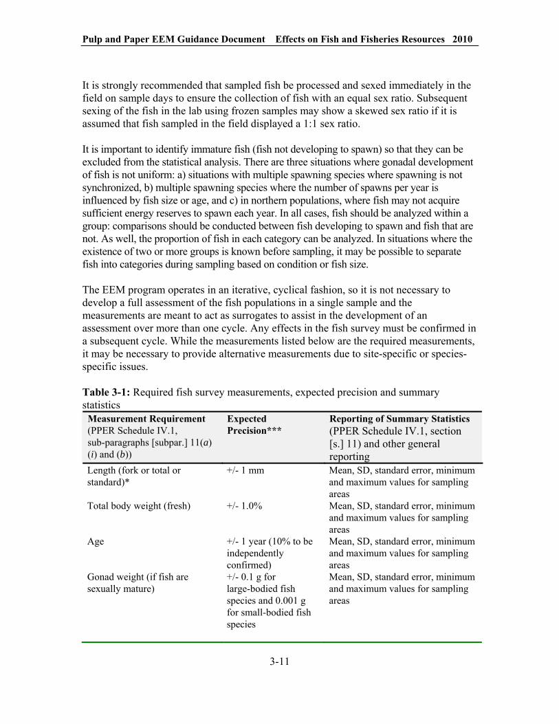
Pulp and Paper EEM Guidance Document Effects on Fish and Fisheries Resources 2010
3-11
It is strongly recommended that sampled fish be processed and sexed immediately in the field on sample days to ensure the collection of fish with an equal sex ratio. Subsequent sexing of the fish in the lab using frozen samples may show a skewed sex ratio if it is assumed that fish sampled in the field displayed a 1:1 sex ratio.
It is important to identify immature fish (fish not developing to spawn) so that they can be excluded from the statistical analysis. There are three situations where gonadal development of fish is not uniform: a) situations with multiple spawning species where spawning is not synchronized, b) multiple spawning species where the number of spawns per year is influenced by fish size or age, and c) in northern populations, where fish may not acquire sufficient energy reserves to spawn each year. In all cases, fish should be analyzed within a group: comparisons should be conducted between fish developing to spawn and fish that are not. As well, the proportion of fish in each category can be analyzed. In situations where the existence of two or more groups is known before sampling, it may be possible to separate fish into categories during sampling based on condition or fish size.
The EEM program operates in an iterative, cyclical fashion, so it is not necessary to develop a full assessment of the fish populations in a single sample and the measurements are meant to act as surrogates to assist in the development of an assessment over more than one cycle. Any effects in the fish survey must be confirmed in a subsequent cycle. While the measurements listed below are the required measurements, it may be necessary to provide alternative measurements due to site-specific or species-specific issues.
Table 3-1: Required fish survey measurements, expected precision and summary statistics
Measurement Requirement (PPER Schedule IV.1, sub-paragraphs [subpar.] 11(a) (i) and (b))
Expected Precision***
Reporting of Summary Statistics (PPER Schedule IV.1, section [s.] 11) and other general reporting
Length (fork or total or standard)*
+/- 1 mm Mean, SD, standard error, minimum and maximum values for sampling areas
Total body weight (fresh) +/- 1.0% Mean, SD, standard error, minimum and maximum values for sampling areas
Age +/- 1 year (10% to be independently confirmed)
Mean, SD, standard error, minimum and maximum values for sampling areas
Gonad weight (if fish are sexually mature)
+/- 0.1 g for large-bodied fish species and 0.001 g for small-bodied fish species
Mean, SD, standard error, minimum and maximum values for sampling areas

Pulp and Paper EEM Guidance Document Effects on Fish and Fisheries Resources 2010
3-12
Egg size (if fish are sexually mature)
+/- 0.001 g Weight, (recommended minimum sub-sample sizes of 100 eggs), mean, standard error, minimum and maximum values for sampling areas
Fecundity** (if fish are sexually mature)
+/- 1.0% Total number of eggs per female, standard error, minimum and maximum values for sampling areas
Weight of liver or hepatopancreas
+/- 0.1 g for large-bodied fish species and 0.001 g for small-bodied fish species
Mean, SD, standard error, minimum and maximum values for sampling areas
Abnormalities N/A Presence of any lesions, tumours, parasites, or other abnormalities
Sex N/A
* If caudal fin is forked, use fork length (from the anterior-most part to the fork of the tail). Otherwise, use total length, and report type of length measurement conducted for each species. In cases where fin erosion is prevalent, standard length should be used.
** Fecundity can be calculated by dividing total ovary weight by weight of individual eggs. Individual egg weight can be estimated by counting the number of eggs in a sub-sample. The sub-sample should contain at least 100 eggs.
*** For small-size fish weights, use at least a 3-decimal scale.
3.4.1.1 Survival
Mean age is meant to give an assessment of the relative ages of the reference and exposed populations. If size-selective gear such as gillnets are used, and there is a significant difference in mean ages of fish sampled at both sites with identical gear, the difference indicates a need to further investigate the population and the reason for the difference in subsequent cycles. More detailed information can be obtained through age distributions (or size distributions if aging is not possible), if adequate sample sizes are available or if aging is not possible. Furthermore, since many fish species have short life spans (< 4 years), it may be necessary to obtain immature fish and juveniles in order to conduct an appropriate assessment of this effect indicator. It is also very difficult to obtain a 25% difference in age when species are short-lived, and it may be possible to substitute a difference in average size (length) of 25% as a surrogate for age when species are short-lived.
A list of appropriate aging structures for a variety of potential sentinel species is provided in Table 3-2. In addition, there are many references that can be referred to for aging methods (e.g., Mackay et al. 1990). Methods of aging should be consistent at each sampling area and among cycles, and appropriate quality assurance / quality control (QA/QC) procedures followed (e.g., independent confirmation). It is recommended that all aging structures be archived for future reference. If fish cannot be aged reliably or if it

Pulp and Paper EEM Guidance Document Effects on Fish and Fisheries Resources 2010
3-13
is not cost- or time-effective, the age can be determined by using size-frequency distributions. This may be especially useful when sampling small-bodied fish species or when conducting non-lethal sampling. It may also be possible to confirm the size-frequency distributions by aging representative sub-samples from each size class. For more information on size-frequency distributions, consult Nielsen and Johnson (1983).
3.4.1.2 Energy Use (Growth and Reproduction)
Growth and reproduction measures give an assessment of the ability of fish to use the food available to them. Growth is the change in size (weight or length) with time or age. In the case of growth, it may be helpful to collect information on other age classes, such as whether there are changes in growth of early life stages. This will assist in determining the magnitude of the effect. Subsequent cycles should focus on confirming responses detected and examining the relevance of the changes to other size classes and species.
Reproduction is expressed as reproductive effort, fecundity, egg weight or gonad weight relative to body size. Reproduction may be the most sensitive measurement in resident fish. Changes in reproductive investment can be evident within a year, because the reproductive tissue is generally turned over annually. Fecundity and gonad weight are easy to measure if an appropriate sampling time is chosen. Confirmed changes in gonad size could lead to additional work related to magnitude, such as determining whether the change occurs at other times of the year (for multiple spawners) or whether the changes are present in other species in the same area.
Table 3-2: Suggested aging structures for Canadian fish species Structure Family (common name/species) Comments Dorsal spine Squalidae (Dogfish Shark)
Dorsal spines or scales Percidae (Yellow Perch) Spines more precise for older fish
Otoliths Anguillidae (freshwater eel), Atherinidae (silverside), Batrachoididae (toadfish), Carangidae (jacks), Clupeidae (herring), Haemulidae (grunt) Gasterosteidae (stickleback), Percopsidae (Trout-perch), Cottidae (sculpin) Gadidae (codfish, Burbot) Preferred; pectoral fin rays
are difficult to age Otoliths, fin ray Scombridae (mackerel)
Otoliths, first four marginal pectoral fin rays, scales
Coregoninae (whitefish)
Otoliths, pectoral fin ray
Acipenseridae (sturgeon)
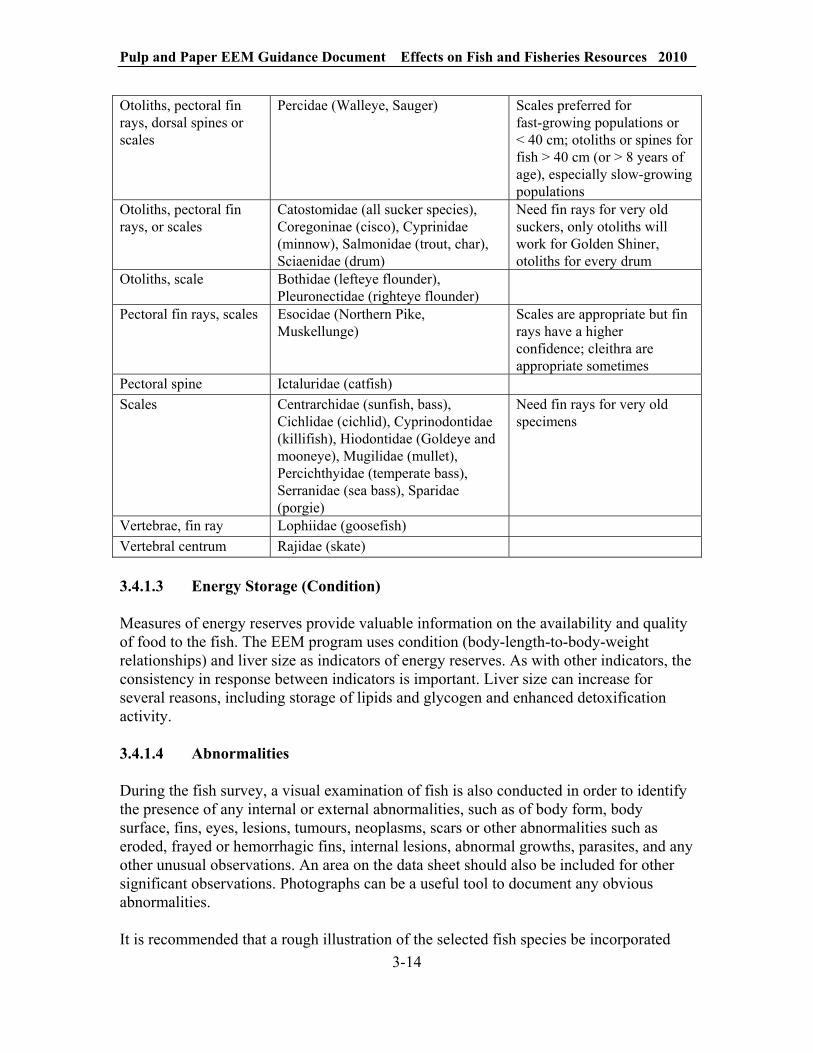
Pulp and Paper EEM Guidance Document Effects on Fish and Fisheries Resources 2010
3-14
Otoliths, pectoral fin rays, dorsal spines or scales
Percidae (Walleye, Sauger) Scales preferred for fast-growing populations or < 40 cm; otoliths or spines for fish > 40 cm (or > 8 years of age), especially slow-growing populations
Otoliths, pectoral fin rays, or scales
Catostomidae (all sucker species), Coregoninae (cisco), Cyprinidae (minnow), Salmonidae (trout, char), Sciaenidae (drum)
Need fin rays for very old suckers, only otoliths will work for Golden Shiner, otoliths for every drum
Otoliths, scale Bothidae (lefteye flounder), Pleuronectidae (righteye flounder)
Pectoral fin rays, scales Esocidae (Northern Pike, Muskellunge)
Scales are appropriate but fin rays have a higher confidence; cleithra are appropriate sometimes
Pectoral spine Ictaluridae (catfish)
Scales Centrarchidae (sunfish, bass), Cichlidae (cichlid), Cyprinodontidae (killifish), Hiodontidae (Goldeye and mooneye), Mugilidae (mullet), Percichthyidae (temperate bass), Serranidae (sea bass), Sparidae (porgie)
Need fin rays for very old specimens
Vertebrae, fin ray Lophiidae (goosefish)
Vertebral centrum Rajidae (skate)
3.4.1.3 Energy Storage (Condition)
Measures of energy reserves provide valuable information on the availability and quality of food to the fish. The EEM program uses condition (body-length-to-body-weight relationships) and liver size as indicators of energy reserves. As with other indicators, the consistency in response between indicators is important. Liver size can increase for several reasons, including storage of lipids and glycogen and enhanced detoxification activity.
3.4.1.4 Abnormalities
During the fish survey, a visual examination of fish is also conducted in order to identify the presence of any internal or external abnormalities, such as of body form, body surface, fins, eyes, lesions, tumours, neoplasms, scars or other abnormalities such as eroded, frayed or hemorrhagic fins, internal lesions, abnormal growths, parasites, and any other unusual observations. An area on the data sheet should also be included for other significant observations. Photographs can be a useful tool to document any obvious abnormalities.
It is recommended that a rough illustration of the selected fish species be incorporated

Pulp and Paper EEM Guidance Document Effects on Fish and Fisheries Resources 2010
3-15
into the data collection sheet for the recording of abnormalities in the external appearance. This information can then be used by others at a later date if significant differences exist between reference and exposure areas.
More information on fish anatomy can be found in general fish biology textbooks. Instructions on tumour descriptions are available in Gross Signs of Tumors in Great Lakes Fish: A Manual for Field Biologists (www.glfc.org/tumor/tumor1.htm).
Table 3-3: Fish survey effect indicators and endpoints for various study designs Effect Indicators
Lethal Effect and Supporting Endpoints
Non-lethal Effect and Supporting Endpoints
Sentinel Mollusc Effect and Supporting Endpoints
Survival *Age*Age-frequency distribution Length-frequency distribution
*Length-frequency distribution Age-frequency distribution (if possible)
*Length-frequency analysis
Growth *Size at age (body weight at age) Length at age
*Length of YOY (age 0) at end of growth period *Weight of YOY (age 0) at end of growth period Size of the 1+ fish Size at age (if possible)
Whole animal wet weight Shell length and width Soft tissue fresh weight
Reproduc-tion
*Gonad weight at body weight Gonad weight at length Fecundity (number of eggs/female at body weight, length, and/or age)
*Relative abundance of YOY (% composition of YOY) YOY survival
*Gonad weight at body weight (gonadosomatic index [GSI]) (bivalves only)
Condition *Body weight at length *Liver size at body weight Liver weight at length Egg weight at body weight and/or age (mature females only)
*Body weight at length *Weight (whole animal dry weight, dry shell or soft tissue weight) related to shell length Soft tissue weight related to shell weight Soft tissue weight related to shell volume
*Fish survey effect endpoints used for determining effects as designated by statistically significant differences between exposure and reference streams. Other supporting endpoints can be used to support analyses.
3.4.2 Non-lethal Sampling
Non-lethal sampling should only be used in situations where it is warranted, i.e., where there is a concern about the potential impacts of sampling on small fish populations. Lethal sampling of adults is preferred where possible, although information on non-lethal samples can be valuable when large numbers of fish are collected during the sampling procedures. The indicators used for non-lethal sampling are contained in Table 3-3, and additional information on statistical analysis for the non-lethal sampling is contained in

Pulp and Paper EEM Guidance Document Effects on Fish and Fisheries Resources 2010
3-16
Chapter 7.
If the only option for a facility is to do a non-lethal sampling of fish in order to evaluate the effects of effluents on the fish population at a facility, a minimum of 100 fish older than YOY is recommended from each study site. The YOY acquired during the collection for the 100 non-YOY fish should also be retained and sampled (measured). YOY can usually be separated from older age-classes by size distributions; however, this may not be possible for species with extended spawning periods. The proportion of fish that are YOY should be estimated from the first 100 fish collected. If YOY abundance is extremely high (> 80-90%), sampling should then continue until 100 non-YOY are captured to calculate size-distributions of older fish. The collection of the additional non-YOY fish allows for a higher discrimination of the older fish classes to be achieved. The fish older than YOY that are collected should represent the whole range of fish sizes and be representative of the population (mature and immature). The recommended sample sizes in each area will give a good idea of the population distribution when plotting parameters such as the length or weight frequency. As well, when examining differences between the relative abundance of young versus mature fish, fairly good resolution is achieved (Gray et al. 2002).
When possible, sampling should be conducted when YOY are a catchable size in the gear being used. The same sampling gear should be used in both the exposure and reference areas; if it is not possible to use the same gear, or multiple gears must be used, the size-distributions within a site should be compared between gears. If there are differences in the sizes of fish collected with different gear, comparisons between sites should be restricted within gear type. The sampling techniques and relative effort should be the same in all sampling areas. Pooling of data from different fish-sampling techniques should be avoided, and all methods used should be reported. If more than one gear type is used, the records of fish caught by each method should be reported, and any pooling of data clearly described. Fish should be measured for length (±1 mm), weight (± 0.01 g) (Gray and Munkittrick 2005), assessed for the presence of abnormalities, and external sex determination should be made, if possible. All fish should then be released. If possible, a small number of larger fish should be sacrificed to verify ages of older individuals. If only adults are used, the priority should be to sample prior to or at the start of the spawning season (see guidance on preferred sampling times in Table 3-5). However, if YOY are to be collected, the timing should move to the late fall, when it will be easier to measure YOY for most species. Fall sampling of YOY will be much more difficult if the fish are not single, synchronous spring spawners, as the size distributions of YOY fish will be broad.
A large number of areas can typically be sampled when conducting a non-lethal survey and the facility is encouraged to sample multiple exposure and reference areas. Programs that sample adults and YOY will allow for maximal assessment of effect indicators.
Species selection for non-lethal sampling can be difficult and is often based on availability. When choices are available, a synchronous spring spawner will offer the most advantages in terms of differentiating YOY from older year-classes. Discrimination of year-classes can also be affected by the longevity of the species. An annual species such as silverside will have a single year-class, eliminating the need to differentiate year

Pulp and Paper EEM Guidance Document Effects on Fish and Fisheries Resources 2010
3-17
classes. A short-lived species (2-3 years) with fast growth and easily distinguished year classes also offers advantages. However, these species are not always available.
When multiple species are available to choose from, it is recommended to collect initial samples and examine the ability to discriminate YOY and age-classes between species.
3.4.2.1 Survival (Size Distributions)
There are challenges to using age information on many short-lived species of fish. If a fish only lives 2-3 years, it will not be possible to measure a 25% difference in mean age. If non-lethal aging structures have not been validated for the sentinel species being used, size-distribution should be examined as a surrogate for differences in age. Size-distributions should be compared between exposure and reference areas with the Kolmogorov-Smirnov test, although this test is not very sensitive. Size comparisons should also examine distributions for YOY alone, for both sizes combined. If a site difference is present, subsequent cycles should focus on understanding the difference and possible causes. When possible, verifying the ages of larger fish and YOY can be useful.
3.4.2.2 Energy Use
It should be possible at most sites to get estimates of growth and reproduction using non-lethal methods. Growth can be evaluated by the size of YOY at the end of the growing season and by the size of the 1+ fish. A comparison of the size of YOY fish between sites gives a good indicator of growth, as it is a direct indicator, in comparison to size-at-age, which is indirect. YOY are used because all of their growth is attributable to environmental conditions since the spawning time, and growth is not complicated by diverging energy into reproductive development. Differences between sites in spawning times will be integrated into this analysis. It is also possible to get a growth estimate by a shift in size distributions over time (e.g., repeating measurements 2 months apart at the same sites), or differences in average size (this would require a second sampling trip to determine). If the fish species chosen is externally sexually dimorphic, it is possible to examine whether there are gender-specific differences in growth rate.
Reproduction can be assessed using relative age-class strength or by the relative abundance of YOY individuals (Gray et al. 2002) or by YOY survival, which requires two sampling periods. A length-frequency distribution may be plotted as a surrogate of an age-frequency distribution. Size-frequency analysis can be used to examine size distributions and distributions of condition factors (using length and weight data), and can be used to infer age distributions and size-at-age data (if ages can be inferred) (Gray et al. 2002). It is recommended that, if possible, aging structures be collected from a sub-sample of each size class, for situations where age may need to be verified (as in section 3.4.1.1, the utility of the age information is reduced in situations where the species is short-lived). In Slimy Sculpin, rapid growth of YOY fish in the spring can cause some overlap with the 1+ age-class, making resolution difficult (Gray et al. 2002). The ability to discriminate the YOY will depend on the duration of the spawning season, and the amount of time elapsed between the spawning time and sampling time. It may be easiest (for

Pulp and Paper EEM Guidance Document Effects on Fish and Fisheries Resources 2010
3-18
spring and early-summer spawning species) to examine length-frequency distributions using late summer and early fall data, when the YOY should be easiest to distinguish. To test for differences in relative abundance of YOY between the exposure and reference areas, a Kolmogorov-Smirnov test can be performed on length-frequency distributions with and without the YOY included. If inclusion of the YOY changes the interpretation of the significance of the difference (i.e., it is different with them included, and not different without them), there is then a difference in the relative abundance of YOY. Alternatively, replicate areas can be sampled to allow for the use of more statistical approaches, or the proportions of YOY can be tested using a Chi-squared test.
It may not be possible to distinguish YOY in species that spawn multiple times, in northern areas where YOY may emerge later in the year, or in situations where there are habitat-preference differences that are age-dependent in a species. In those cases it will not be possible to easily infer potential reproductive impacts. Some professional judgement will be required. If the species lives multiple years and immature fish can be distinguished non-lethally (condition near spawning time can be used in many situations for this), the proportion of immature fish can be used as a substitute. In cases where this is not possible, interpretation will need to be made based on size distributions alone, and care must be exercised to be conscious of the potential impacts of adult mortality on interpretation.
It is important to remember that a difference in water temperature between sites will affect spawning time. End-of-summer differences in size distributions could as easily result from differences in spawning time due to temperature as other potential causes. If there are temperature differences between sites that are suspected to be a major cause in the differences in size-distribution observed, then subsequent studies should determine whether these site differences are a consequence of the facility or an inadequacy in choosing reference sites.
If it is possible to make multiple sampling trips, it may also be possible to measure changes in condition before and after spawning as an indicator of reproductive investment. For some small-bodied species, spawning females are very easy to distinguish by condition factor. Differences in condition factor of females between sites before spawning, or an indication of the change before and after spawning in females, could be used to infer reproductive investment, if females can be distinguish after spawning.
3.4.2.3 Condition
Condition factor (k) can be evaluated by the relationship (k = 100 000* (wt/l3)) of the fish examined (where wt = weight [in grams] and l = length [in mm]). The appropriate analysis for final interpretation is an analysis of covariance (ANCOVA) of weight versus length, by site.
3.4.3 Wild Molluscs

Pulp and Paper EEM Guidance Document Effects on Fish and Fisheries Resources 2010
3-19
Where there are no appropriate finfish present, collection of wild molluscs, such as oysters or mussels, may be considered. Shellfish are included under the definition of fish in the Fisheries Act and they have been used by some mills during previous cycles. However, there are some drawbacks, including difficulties in aging individuals and in estimating reproductive investment in some species. Crabs and lobsters are not suitable species because they cannot be reliably aged at the present time (Environment Canada 1997). Currently, guidance is available on the relative gonad index (mantle somatic index) for bivalves (see mesocosm guidance in Chapter 8).
Molluscs are a diverse taxonomic group that include bivalves and gastropods, and are widely distributed throughout Canada. Molluscs possess many qualities that a species for monitoring should exhibit:
they are relatively sedentary, although some species (i.e., unionids) may migrate short distances (metres) within their habitat;
they are widely distributed across Canada and are identified with limited taxonomic expertise;
most unionid bivalves are large enough to provide sufficient tissue for analyses; several bivalve species have been shown to readily accumulate many chemicals
from a variety of pathways (water, sediment, food) and show sublethal effects associated with exposure; and
bivalve growth is relatively easy to measure and has been shown to be as sensitive or more sensitive than mortality in other standard assays on species such as Daphnia, Fathead Minnow and Rainbow Trout (see Salazar and Salazar 2001).
In general, reproductive periods for molluscs and patterns of abundance are related to climate and the abundance of food supply. For most freshwater lotic or lentic habitat types, sampling is best conducted during the fall when the majority of taxa will be present and/or are large enough to be easily collected. In marine environments, sampling should be conducted in late summer or fall, as populations with spring recruits have stabilized by this time.
3.5 Timing of Sampling
A variety of factors need to be considered when deciding on a time to sample, including potential migratory behaviour of the sentinel species, water conditions (e.g., flow, turbidity, wave action), accessibility, and the cycle of gonadal development for the sentinel species. Where historical data exist, it would be useful to examine the data and, if appropriate, conduct the survey during similar periods so that the surveys can be compared.
The timing of sampling should be synchronized with the development of sufficient gonadal tissue so that effects on the reproductive function can be assessed. However, such information is unavailable for many species of fish. Species for which there exists extensive background information on their biology and life history characteristics should

Pulp and Paper EEM Guidance Document Effects on Fish and Fisheries Resources 2010
3-20
be preferred as sentinel species in order to ensure that sampling can be synchronized with sufficient gonadal tissue development.
Recent research has been conducted to evaluate the optimal timing for interpreting gonadal development, using seasonal collections from a variety of species. Five types of fish categorized by spawning characteristics have been identified, and Table 3-4 provides the recommended sampling time based on the following background collection studies: background collections followed Canadian freshwater species that were synchronous spawners (such as Slimy Sculpin; Gray et al. 2005; Brasfield 2007), multiple spawners with few spawnings per year (such as Blacknose Dace [Rhinichthys atratulus]; Galloway and Munkittrick 2006; Hicks and Munkittrick, unpublished data), multiple spawners with many spawns per season (such as Redbelly Dace [Chrosomus eos]; Carroll 2007), and asynchronous spawners (every few days, such as Mummichog [Fundulus heteroclitus; McMullin et al. 2009). There is a fifth type of freshwater species that has asynchronous development, where individuals may take a year off from spawning because of cold temperatures or low food availability. This variability has a major impact on power and sample size requirements.
Examination of these data confirms that there are specific times when power is higher for detecting differences, and when gonadal development is adequate for detecting impacts. The generalizations in Table 3-4 may not apply to all species or all regions; the regional EEM contact should be consulted for any available updates to regional guidance.
Synchronous spawners show a difference in timing of gonadal development between males and females. For synchronous spring spawners, adequate data can usually be obtained as late as possible in the fall, or prior to spawning in the spring. If previous data are available for a site, the reproductive strategy can usually be estimated from the magnitude of the correlation coefficient (R2) between gonad weight and body weight, if the previous collections were done at a time when the gonads were well developed.
Table 3-4: Generalizations and suggested optimal sampling times for fish species in EEM Reproduction Type Sample Time R2 for Gonad Weight vs.
Body Weight Relationship for Reference-site Females
Synchronous spawners Late fall (if spring spawner) Early summer to mid-summer (if fall spawner)
> 0.85
Multiple spawners, few spawns
4-6 weeks before first spawn (usually April to early May)
0.4 < R2 < 0.8
Multiple spawners, many spawns
As close to start of spawning as possible
< 0.4
Asynchronous spawning After spawning has started or near start of spawning period
Not significant
Asynchronous development (year off)
Separate groups and treat independently
Two groups of fish seen with different slopes within a site

Pulp and Paper EEM Guidance Document Effects on Fish and Fisheries Resources 2010
3-21
Multiple spawners with few spawns should be sampled at least 6 weeks prior to the initiation of the spawning season (for information on spawning temperatures, consult references such as Scott 1967; Scott and Crossman 1973; Roberts 1988; Nelson and Paetz 1992; Jenkins and Burkhead 1993; Coad 1995) due to an increased variability in the gonad-weight-to-body-weight relationship as the spawning season approaches, because of a lack of synchronization in timing for the second clutch of eggs (Galloway and Munkittrick 2006). Multiple spawners with many spawns, and asynchronous spawners, should be sampled close to the start of the spawning period because of the rapid development of the gonads in both species.
The consequences of sampling at an inappropriate time have been examined using previous data from cycles 1 to 3. For large-bodied species, fish were sampled outside of the optimal window in more than 33% of previous studies, but interpretation was not strongly affected when optimal and suboptimal studies were compared. However, small-bodied species were sampled at suboptimal times more than 75% of the time, and data collected outside of the optimal windows failed to detect significant effects on gonad or liver size (Barrett and Munkittrick, unpublished data).
Table 3-5: Fish species commonly used in EEM, aspects to consider during study design, and recommended sampling times (based on Barrett and Munkittrick, 2010) Family Species Scientific Name Considerations Sample Salmonidae Lake Trout Salvelinus namaycush F M* 4-6
Brook Trout Salvelinus fontinalis F M A 4-6 Arctic Charr Salvelinus alpinus F M D 4-6* Dolly Varden Salvelinus malma F M? 4-6 Bull Trout Salvelinus confluentus F M? 4-6 Cutthroat Trout Salmo clarki W M* A LF Rainbow Trout Oncorhynchus mykiss S (F) M A LF* Arctic Grayling Thymallus arcticus S M A LF Mountain Whitefish Prosopium williamsoni F M? 4-6 Round Whitefish Prosopium cylindaceum F/W M? 4-6 Lake Whitefish Coregonus clupeaformis F M* 4-6 Cisco Coregonus artedii F 4-6
Hiodontidae Goldeye Hiodon alosoides S M P H SPAW Mooneye Hiodon tergisus S M? LF
Esocidae Northern Pike Esox lucius S M LF
Cyrpinidae Carp Cyprinus carpio X M* 4-6 Fallfish Semotilus corporalis S X? G? LF Creek Chub Semotilus atromacualtus S X* 4-6 Peamouth Chub Mylocheilus caurinus S LFLake Chub Couesius plumbeus S M LF Longnose Dace Rhinichthys cataractae X 4-6

Pulp and Paper EEM Guidance Document Effects on Fish and Fisheries Resources 2010
3-22
Blacknose Dace Rhinichthys atratulus X 4-6Pearl Dace Margariscus margarita X? 4-6Redbelly Dace Chrosomus eos A SPAWSpottail Shiner Notropis hudsonius X? M? 4-6 Mimic Shiner Notropis volucellus X? 2 yr? 4-6 Emerald Shiner Notropis atherinoides X? M? 4-6 Blacknose Shiner Notropis heterolepis X 4-6Common Shiner Luxilus cornutus S? 4-6Golden Shiner Notemigonus crysoleucas X? 4-6Redside Shiner Richardsonius balteatus A? SPAWBluntnose Minnow Pimephales notatus S G 4-6 Fathead Minnow Pimephales promelas A G 4-6
Catostomidae White Sucker Catostomus commersoni S M LFLongnose Sucker Catostomus catostomus S M LFLargescale Sucker Catostomus macrocheilus S M? LF Bridgelip Sucker Catostomus columbianus S M? LFShorthead Redhorse Moxostoma S M LF Sucker macrolepidotum Silver Redhorse Sucker Moxostoma anisurum S M? LF
Ictaluridae Brown Bullhead Ameiurus nebulosus S G 4-6 Channel Catfish Ictalurus punctatus S G D 4-6
Fundulidae Mummichog Fundulus heteroclitus A R SPAW
Gadidae Burbot Lota lota W M? H LF
Atherinidae Atlantic Silverside Menidia menidia S 1 yr. SPAW
Gasterosteidae
Brook Stickleback Gasterosteus aconstans X SPAW*
Threespine Stickleback Gasterosteus aculeatus X M* SPAW* Ninespine Stickleback Pungitius pungitius X M* SPAW*
Percopsidae Trout-perch Percopsis omiscomaycus X M* 4-6
Centrarchidae Rock Bass Ambloplites rupestris S G 4-6 Pumpkinseed Sunfish Lepomis gibbosus S G 4-6 Smallmouth Bass Micropterus salmoides S G 4-6
Percidae Walleye Sanders vitreus S M LF Yellow Perch Perca flavescens S M* H D LF Iowa Darter Etheostoma exile S G M* 4-6 Johnny Darter Etheostoma nigrum S G M* 4-6 Logperch Percina caproides S M* 4-6
Cottidae Mottled Sculpin Cottus bairdii S G LM LF Slimy Sculpin Cottus cognatus S G R LM LF Torrent Sculpin Cottus rhotheus S G LM LF Spoonhead Sculpin Cottus ricei S G LM LF Shorthorn Sculpin Myoxocephalus scorpius W G LF
Note: The best designs for sampling fish fall under three categories: a) close to the start of spawning

Pulp and Paper EEM Guidance Document Effects on Fish and Fisheries Resources 2010
3-23
(SPAW); b) late fall (LF) or about 6 months prior to spawning; and c) 4–6 weeks prior to first spawn (late April/early May). Spawning S - spring or early summer spawners, usually a single spawning time, usually migrate to spawn F - fall spawners, usually single spawnW - winter spawners, usually single spawn X - multiple spawners, usually summer spawners: assess whether small fish are reproducing less (or more) than larger fish (view GSI vs. length); variability will increase as spawning season approaches; best to sample 4–6 weeks prior to first spawn G - males are guarders; reproductive investment in males will be low, but they are likely not very mobile A - asynchronous spawners ? - some doubt about number of spawns: either multiple or asynchronous
Migration M - mobile; are known to migrate considerable distances (or change habitats significantly) for spawning at some sites * - may be site-specific M? - probably migrate A - anadromous forms may be present, and may be much larger and much more mobile C - catadromous; migrate out as adults R - research available to show that they are usually resident
Other P - plankton feeder; migratory feeder 1 yr - 1-year life cycle 2 yr - 2-year life cycle H - juvenile and mature fish may utilize very different habitats LM - females may start to mature very late in the year, fish may spawn during freshet; can be difficult to obtain mature female gonads D - diet changes within the size of sexual maturity, to piscivorous at larger sizes (when available)
3.6 Verification of Fish Exposure
It is crucial that studies be designed to maximize the possibility of detecting effects if they are present. This can be accomplished by sampling at the proper time of year, with appropriate gear, at appropriate reference areas and during the period of residence in the effluent area. If fish exposure to the mill effluent is uncertain, redesigning the survey (selecting different species, using tracers, changing sampling time or changing exposure or reference areas) or using alternative monitoring methods should be considered for the subsequent cycle.
Controversy arises when fish show no differences in characteristics among sites, and there are no indicators of exposure. In this case, it is difficult to determine whether the fish at both sites belong to the same population. In order to verify the exposure of fish to effluent in the exposure areas, and to verify the lack of exposure at reference areas, it may be necessary to select a tracer which accumulates in fish tissue. The selection of a tracer depends on the type of mill involved and the complexity of the receiving environment.

Pulp and Paper EEM Guidance Document Effects on Fish and Fisheries Resources 2010
3-24
Chemical indicators (e.g., chlorophenols) have become less useful as indicators of exposure as mills have improved processes and treatment. Biochemical responses are relatively short-term indicators of very recent exposure histories. Liver detoxification enzymes (mixed function oxygenase [MFO]) may only indicate the exposure history for the previous 3–14 days (Munkittrick et al. 1991, 1994, 1999) and other indicators like bile metabolites of polycyclic aromatic hydrocarbons (PAHs) would be even shorter. Although these measurements can give recent evidence of exposure, longer-term integrators are better.
Large statistical differences between sites in whole-organism characteristics in a number of parameters give some confidence that the samples are from different populations of fish. If there are no differences between sites, it may be that fish are moving or that there is no impact. Stable isotopes of carbon and nitrogen can be used to document that there are differences in fish residence times, provided that the stressors in question locally alter stable isotopes (i.e., Farwell 1999; Galloway et al. 2004), or there are local geochemical differences that alter stable isotopic signatures and that can be used to demonstrate local residency (i.e., Gray et al. 2004). However, the stable isotopes are not always sufficiently different between sites to be useful, and their suitability has to be evaluated on a site-specific basis (Dubé et al. 2006).
By selecting a sampling time and fish species that have life history habits that may increase the likelihood of exposure, potential exposure can be maximized. For example, for species having spawning movements that take them away from or temporarily into the effluent exposure area, a survey conducted during the spawning season would be ineffective. Thus, for spring-spawning freshwater species, a fall survey would be appropriate. For fall spawners, a spring or summer survey is appropriate. This may not apply to fish in which ova mature rapidly; for example, as some late-spring-spawning cyprinids should be sampled in early spring, rather than in fall when ova may still be immature, it is pertinent to have some background biological information, if possible.
The timing of sampling and the choice of fish species should be made according to normal operation of the facility to ensure that the effluent is present in the environment. Sampling when effluent has not been discharged for long periods (months) should be avoided. However, the selected sampling gear, flow conditions and effluent conditions may limit the preferred season for the survey.
If no fish are captured (or they are captured in reduced density) and there are no fish resident in the exposure area, it could be interpreted that fish are avoiding the exposure area. The suitability of fish species should be evaluated at the end of each monitoring cycle, based on the site-specific nature of the results and the site-specific concerns about residency and exposure.
There are some situations where fish may move freely in and out of the exposure area, and no species spend significant periods of time in the effluent. In these cases, the sampling should be designed to maximize exposure time in the effluent area and possibly during periods of optimal gonadal development.

Pulp and Paper EEM Guidance Document Effects on Fish and Fisheries Resources 2010
3-25
There are two main issues dealing with residency: whether the fish from reference and exposure areas were mixing; and whether the fish captured in the exposure area were indeed exposed. If fish demonstrate exposure, are collected in the exposure area, and demonstrate differences from reference-area fish, there should be no controversy. Follow-up studies can examine other species to see if they demonstrate effects.
If fish demonstrating exposure, are collected in the exposed area, and show no differences, it is outside the scope of the EEM to determine why exposure-area effects are not seen. If subsequent monitoring cycles confirm the absence of demonstrated effects and the study design was adequate, it would be concluded that the conditions of the area allow for fish that are exposed to effluent not to be affected, using the current design.
3.7 Power Analysis
The purpose of defining an effect-size and power level is to determine if the sampling program is collecting sufficient information for decisions to be made. The statistical power of a comparison is a function of the sample size, the variability and the target difference set between areas. To determine the sample size for detecting a specific difference, some knowledge is needed about the statistical power level that is acceptable for the decision-making process and the variability of the population.
3.7.1 Power and Significance Level
Earlier cycles of EEM set the power (1-beta [β]) at 0.80 and alpha (α) at 0.05. Since Cycle 3, mills were encouraged to set α and β equal to one another. If values are set at α = β = 0.10, the sample sizes required to detect the same effect are approximately the same as in earlier cycles. Where possible, provided sample sizes determined by the power analysis are not unreasonably large, mills are encouraged to reduce α = β = 0.05 (the traditional level for alpha). In many statistical programs, the default β is 0.20, and needs to be adjusted. Again, these recommendations are to help ensure that studies are designed to provide a reasonably high probability of statistically detecting a predetermined effect size if it has occurred, (i.e., the power of the test [1-β] should be high). Refer to Chapter 7 for the rationale for setting α and β at equal levels.
It is important to understand that variability and power will vary with the parameter being studied. Fish are not equally variable across all of their characteristics. Reproductive variables are usually as changeable, or even more on a relative scale, than parameters such as length, weight and liver weight (Environment Canada 1997). If effect sizes are also expressed on a relative scale (i.e., as percent differences), any study that can detect a ± 25% difference in relative gonad size can detect similar or smaller differences in other important parameters.
3.7.2 Effect-Size

Pulp and Paper EEM Guidance Document Effects on Fish and Fisheries Resources 2010
3-26
Consistent with recent cycles, it is recommended that the EEM program be designed to detect a difference of 20-30% in gonad size, using a recommended power level of 0.90 (1-β). The magnitude of the difference that could be detected for other parameters would be fixed based on the sample size for determining an effect on gonad size. The power for detecting differences in other parameters should be reviewed during study design to ensure that reasonable power is achieved for as many variables as possible. The same approach used to identify a target effect-size for relative gonad weight should be applied to other variables. Sensitivity analyses using population models should be used to explore the consequences of the effect-size chosen for any and all variables (Environment Canada 1997).
An extensive literature review has shown that CESs that have been defined in other programs are often consistent with a CES of around 25% or 2 SDs for many biological or ecological monitoring variables. This value appears to be reasonable for use in a wide variety of monitoring programs and with a wide variety of variables (Munkittrick et al. 2009). Barnthouse et al. (1989) argue that a 10% change in variables would be societally and ecologically significant, although they were concerned primarily with laboratory toxicity tests and not field surveys. Their proposed effect-size was deliberately conservative (small) because of concerns about the uncertainty in extrapolating laboratory results to the field.
When preliminary analyses show that power will be insufficient given reasonable sample sizes, the assessments should be redesigned. Studies are designed site-specifically, and priority should be given to reducing variability rather than increasing sample size. As variability will also vary between sampling campaigns, the target effect-size should not be a fixed number, but rather should be a range of changes that you wish to detect, such as 20-30% difference. Sample sizes can be calculated using methods described in Green (1989) and Environment Canada (1998); sample size calculators can also be downloaded from the Internet, such as the common one that can be found at http://biostat.mc.vanderbilt.edu/wiki/Main/PowerSampleSize.
A priori power calculations and CES calculations are described in section 7.6.2.1 of Chapter 7.
3.8 Fish Sampling Methods
Sampling methodology should be chosen site-specifically, and capture gear and effort should be focused on methods shown to be successful. The same sampling methods can be used for population and community surveys. The difference lies with the selectivity of the fishing gear. During a community survey, the gear should be as non-selective and non-destructive as possible. For the population survey, which focuses on one or two species, the gear will be more selective. For example, trap netting may be preferred during a community survey while a one-size mesh gillnet of the appropriate size could be appropriate for a population survey.

Pulp and Paper EEM Guidance Document Effects on Fish and Fisheries Resources 2010
3-27
Standardized sampling is a priority. Therefore, in situations where sentinel species are the same as for a previous cycle, and the sampling techniques used previously were sufficient to capture the target number of each sentinel species, these same sampling techniques should be retained unless good reasons for change, such as unacceptable bycatch, are documented. The sampling techniques and relative effort should be the same in all sampling areas. Pooling of data from different fish-sampling techniques should be avoided, and all methods used should be reported. If more than one gear type is used, the records of fish caught by each method should be reported, and any pooling of data clearly described.
A number of good guidance documents fully describe fish collection methods (Schneider 2000; Portt et al. 2006). Portt et al. (2006) describe the use and efficacy of 1) gillnets; 2) beach seines; 3) hoop, fyke and trap nets; 4) electro-fishing; 5) underwater observation; 6) Gee or minnow traps; and 7) enclosure (drop, pop and throw) traps. However, methods will usually have to be developed and optimized site-specifically.
3.8.1 Bycatch
It may be possible to obtain samples using the bycatch of commercial, research or other fisheries operations in either marine or freshwater situations. The investigator is responsible for ensuring and documenting that sampling procedures and conditions are met (QA/QC), and that fish are exposed. Capture techniques also have to be standardized between sites.
3.8.2 Remote Sensing
Fish abundance near outfalls can be monitored using video or still cameras mounted on remotely operated vehicles. This technique may be particularly effective in rocky and steep areas where use of fishing gear may be difficult. Camera surveys may also be useful in reconnaissance surveys of bottom conditions before trawls or traps are deployed for fishing. Any proposed methods should be clearly outlined in the study design for review.
3.8.3 Alternative Methods
Given the variety of problems and situations at each pulp and paper mill, there may be cases where the fish survey is not suitable. The reasons for this are site-specific, but the most common reasons are the presence of hazardous conditions (e.g., strong currents) or the presence of confounding factors such as other effluent discharges in the exposure area, which will make it difficult or impossible to isolate any effects attributable to the effluent being monitored. Under these circumstances, the mill may select an alternative option to the fish survey and/or the fish usability survey. Recommended alternative monitoring methods for the fish survey are mesocosm studies and caged bivalves. Detailed guidance on how to conduct the alternative monitoring methods and interpret the data can be found in Chapter 12.

Pulp and Paper EEM Guidance Document Effects on Fish and Fisheries Resources 2010
3-28
3.9 Fish Survey Quality Assurance and Quality Control
3.9.1 Field Practices to Improve Data Analysis and Interpretation
The quality of data collected in the field influences the ease of data analysis and interpretation. The preparation of data recording sheets beforehand will save time in the field and the use of waterproof paper is encouraged. Field conditions, habitat, gear used and information for catch-per-effort calculations should be recorded. The use of the same balance and measuring device for all measurements, and having the same person taking the measurements, will reduce measurement error. If the person taking the measurements is reporting the data to a person recording the measurements, avoid the use of decimal points and report all measurements as digits and not numbers to avoid transcription errors (e.g., report 14.5 cm as 1-4-5 and use units of mm); some numbers can be easily confused when reported orally, such as “fourteen” vs. “forty.”
It is essential that the sampling gear be consistent between the sampling areas, because most sampling methods select for certain age- or size-classes, and thus inconsistent sampling gear between sampling sites could result in detecting false differences (e.g., in age or size).
3.9.2 Quality Control in the Field
This is the first stage of data collection. QA/QC procedures for the fish survey should be outlined during the development of the study plan and should be followed precisely in order to maintain high-quality data. While a QA/QC plan for field sampling can have many components, some of the main procedures are as follows:
initiate and maintain communication with local government agencies (e.g., fishing licence, dates of fish collection, location of collection, endangered species, etc.);
all personnel involved in field sampling should have appropriate education and/or training and be familiar with the written standard operating procedures for the survey;
all safety measures should be identified, understood and adhered to; fish collection methods and equipment should be appropriate for the specific water
body and fish species; habitat descriptions, including possible modifying factors (water depth and
current, dissolved oxygen concentration, temperature, substrate classification, evidence of pollution [discolouration, odour, residues], salinity, conductivity, etc.);
date and time of collection; collection methods need to be consistent throughout the study; location of sampling areas and fish collection areas documented (geographic
coordinates); photograph the collection location; record of the number of fish species and incidental species caught per collection

Pulp and Paper EEM Guidance Document Effects on Fish and Fisheries Resources 2010
3-29
stations; estimate of catch per unit effort; samples from fish (e.g., ovaries, age structures) should be placed in appropriate
containers; suitable preservatives/fixatives (e.g., ovaries—frozen or formalin) should be used; all samples should have appropriate labelling; all measurements will be taken using appropriate equipment of acceptable accuracy
and precision (this should be documented); instruments should be calibrated and maintained in good working order (records and
methods should be available); detailed field notes should be maintained in a bound notebook; and chain-of-custody forms and appropriate shipping and storage procedures should be
used.
3.9.3 Determination of Sampling Effort
To aid in assessment of expected effort requirements at individual sites, the study plan submitted to Environment Canada should include details on how fish sampling will be performed.
The following are performance-based criteria and guidance to determine a “reasonable level of fishing effort.” Each site is unique. It is uncertain whether fishing success will be achieved at a site just because a certain level of sampling effort has been successful in the past at other sites or even at the same site at other times.
1. The study design should document all details on how the adult fish sampling will be performed, to aid in assessment of effort. Details to include in the study design (where applicable) are:
how and why the sentinel species were selected; who was consulted on the locations and techniques chosen to collect the proposed
sentinel species; contingency plans regarding alternative gear and sentinel species; scheduling of dates for work that will be performed so that EEM contacts can be
available for consultation; type, location(s) and dimensions of gear (e.g., gillnet, trapnet, hoopnet, fish trap,
trawl; in some cases more than one type of gear may be advisable); mesh type (e.g., nylon, cotton fibre or wire, knotted or knotless) and size; proposed level of gear / fishing effort; sampling time (i.e., time of day); sampling duration (i.e., time interval between gear placement and retrieval); and frequency of checks.
Any preliminary fish survey results or observations made during pre-design activities should be provided where they have guided selection of sentinel species or

Pulp and Paper EEM Guidance Document Effects on Fish and Fisheries Resources 2010
3-30
procedures. The regional EEM contact will review these data and may request further information to clarify sampling procedures.
2. Proper operating procedures should be used. These include use of gear as outlined in the study plan. Gear should be checked at a frequency that ensures the recovery of sentinel species in useful condition and the release of non-target (especially protected and endangered) species. The use of non-lethal and/or selective techniques should be a consideration. A record of the identity and estimated numbers of non-target fish may be a useful addition to contingency plans. The mill and consultant should have a good understanding of the habitat, the characteristics of the species, and the gear being considered.
3. Consultation with local experts (e.g., provincial and federal fisheries personnel, Aboriginal groups, individuals and associations involved in local sport and commercial fisheries, the public, and others with knowledge of local fisheries resources) should be conducted to ascertain that the selection of sentinel species, location of nets, timing of collections, etc., are optimal.
4. Personnel tasked with the fish collection and sampling procedures should have documented experience.
5. Licences for collecting should be obtained from local fisheries agencies.
6. Records should be kept that document the operating procedures used (e.g., mesh size, sampling time, location, frequency of checks, etc.). These records may be required in order to properly assess the manner in which the study was conducted.
Although not required, it is recommended that an estimate of catch per unit effort (CPUE) be provided for each sampling area (e.g., number of fish caught per unit of time or area or net). The CPUE information is useful in documenting the effort expended in situations where collection of the minimum number of fish may be difficult.
3.9.3.1 Examples of Calculations of Sampling Effort
Some examples of fishing methods that have been successful in collecting fish in a timely manner are provided below. These are provided as examples to guide consultants in the development and implementation of their study design, and to indicate when it may be advisable to consult with the Environment Canada regional EEM coordinator.
1. Data from two Ontario lakes indicated that 40 individuals of any of 6 warm-water fish species were collected in 1-6 sets for 24 hours duration. The equipment included a 6-x-6-foot trap net. Details of the process are presented in the Ontario Ministry of Natural Resources Fisheries Assessment Unit Newsletter (FAU Update Issue 94-1, 1994).
2. During the Assessment of the Abundance of Cold Waters Ontario Fish Communities

Pulp and Paper EEM Guidance Document Effects on Fish and Fisheries Resources 2010
3-31
Program, the fishing effort recommended to collect 40 Lake Trout in 7 lakes varied from approximately 12 to 120 hours. The equipment included a 46-m gillnet gang with 3 panels of 15.2 m. Details of the process are in the Ontario Ministry of Natural Resources Fisheries Assessment Unit Newsletter (FAU Update Issue 94-2, 1994). Mesh size should be consistent and selected according to the target species.
3. Experience has shown that gillnets made up of 4 panels of 50 m of net, set 24 hours/day for 5 days (equivalent to 24 000 metre-hours of effort) in freshwater systems, should allow for 20 fish of each sex to be collected. This is contingent on correct deployment of the panels and shifting of the panels to cover areas inhabited by the fish. Mesh size should be consistent and selected according to the target species.
4. Alternatively, a good strategy would be to initially set a minimal amount of net to decrease bycatch (< 400 m). If fishing is selective enough, and the amount of bycatch acceptable, up to 2 km of a single mesh size has been necessary in small unproductive rivers.
5. In marine situations, experience has shown that 48 hours of beam trawling, long-lining using a variety of hook sizes or other methods including traps (alone or in combination), should provide the 20 fish of each sex.
6. Consultation with users of electro-fishing technique (large rivers using boat-mounted apparatus) indicates that all fish can be obtained in one day. Procedures enhancing success include operating at dusk or night, passing over the same area at least three times, and using intermittent pulses of current (since a continuous field may actually chase fish away). In small streams, lakes and rivers, more time will often be necessary for sampling because of the difficulties encountered in moving through these environments.
7. In 1999, a consultant was collecting fish for an East Coast paper mill located on a tidal estuary. The target species were Mummichogs and the consultants used a 15-x-1.5-m beach seine with 0.5-cm mesh. One end of the beach seine was extended about 10 m out from shore by a technician wearing chest waders, while a second technician held the other end of the seine along the shore. The technicians towed the seine perpendicular to the shore for a distance of 20-30 m and then the outer end was towed into the shore to close the net. Once both ends of the seine were secured on the shore, the upper and lower lines were carefully retrieved to capture any fish enclosed in the net. The consultants found that fishing was most successful at slack high tide. A total of 108 Mummichogs were captured and retained over 4 days of sampling. Total fishing time was 12.5 hours. Many more Mummichogs were captured and released due to the need to balance male and female numbers. In addition, 11 other species of fish were captured and released (Final Report, Repap New Brunswick Inc. Kraft Mill, Second Cycle Aquatic EEM Study, Jacques Whitford Environment Limited, April 2002).

Pulp and Paper EEM Guidance Document Effects on Fish and Fisheries Resources 2010
3-32
Although the above techniques and gear may apply to a variety of species, these examples are not all-inclusive because each site is unique and the examples are provided as suggested effort only. Local expertise can serve as further advice. The previous examples are adequate guidelines toward catching a minimum of 20 fish per sex, species and area.
3.9.4 Consultation with Regional EEM Coordinators and Implementation in the Field
If all of the above criteria are met and a mill/consultant is having problems meeting the minimum data requirements of the adult fish survey, the owner or operator may deviate from the study design but is required to inform the Authorization Officer without delay of those circumstances and of how the study was or will be conducted. All reasonable efforts should be made to collect target sample sizes of two species of fish and demonstrate due diligence on the part of the mill.
Possible outcomes and options of the consultation with the EEM coordinator are as follows:
1. Continue – Advice on the following situations will depend on site-specific conditions. Set further consultation dates if required.
a) Absence of target species at reference area: continue with current gear and technique; continue at alternative reference area identified in contingency plan; continue at existing reference area with alternative target species, gear
and/or technique identified in contingency plan. b) Absence of target species at exposure area:
continue with current gear and technique; continue at alternative exposure area identified in contingency plan; continue at existing exposure area with alternative target species, gear
and/or technique identified in contingency plan. c) Absence of target species at reference and exposure areas:
continue with alternative areas, target species, gear and/or technique identified in contingency plan.
2. Postpone (not to continue) – Existing dangerous conditions; sampling conditions (e.g., weather, cold) will not allow collection of fish; alternative gear is not available; no further contingencies are available (e.g., no further alternative species; further investigation is needed):
design new sampling plan in consultation with regional EEM contact; redeploy at a later date with original or alternative areas, target species, gear
or technique, but under more favourable conditions; set dates for further consultation.
3. Discontinue – If the full complement of fish is not obtained, the absence (or paucity)

Pulp and Paper EEM Guidance Document Effects on Fish and Fisheries Resources 2010
3-33
of fish will be considered a result that will be thoroughly explained in the study findings, taking all possible contributing factors into account. If the minimum number of fish is not caught, this could result in inflated variance estimates. The decision on whether to continue will be influenced first by safety considerations. In all scenarios refer to the contingency plan where appropriate, and set date(s) for further discussion. Field technicians should speak directly with the regional EEM contact. Sentinel species choices will apply to both reference and exposure areas. Pooling of data from different seasons is not valid.
3.9.5 Data Entry
Data entry and preparation of analysis is discussed in Chapter 7, and reporting is discussed in Chapter 9.
3.9.6 Quality Control in the Laboratory
Although much of the survey information is collected while in the field, variables such as fecundity, egg weight, and age are usually determined later in the laboratory. With each measurement, the primary concern of the laboratory QA/QC program is to ensure consistency (precision) and accuracy of the data. The following issues should be considered as part of the measurement procedures:
all personnel involved in sample processing and analyses should have appropriate education and/or training;
measurements should be conducted using recognized protocols and methods (these should be documented), and all instruments used should be properly calibrated and maintained (records, methods available);
keep fish measurements recorded for each fish (target species); keep a record of external lesions, tumours, parasites, etc; fecundity data, including methods and sub-sampling precision (if applicable); aging data, including methods and independent confirmation of estimates; maintain records that describe the sample, measurement, and responsible personnel;
if possible, a minimum number of individuals should conduct a particular measurement to maintain consistency and reduce measurement error (especially for age determination);
if sub-sampling is necessary (e.g., fecundity, egg weight), information describing the efficiency and accuracy of the sub-sampling technique should be documented; this information should also be used to calculate appropriate correction or scaling factors (if needed) to minimize possible differences in methods and efficiency;
all data should be verified; for example, measurements such as fecundity and egg weight should be replicated to ensure precision and accuracy; a recognized expert should verify estimates of age;
literature and taxonomic keys used for fish identification should be documented; archive samples and voucher specimens; and maintain detailed sample processing and laboratory notes in a bound notebook.

Pulp and Paper EEM Guidance Document Effects on Fish and Fisheries Resources 2010
3-34
3.10 Data Analysis
QA/QC concerns regarding data analysis include data verification and validity, repeatability and robustness of statistical analyses, and rigour and defensibility of analyses. For the most part, validation and verification of data depends on the success of QA/QC procedures during field sampling, sample processing, and laboratory analyses (see above). However, there are other considerations regarding the data verification and analyses:
conduct screening techniques to identify possible transcription errors, outliers and other potentially questionable data points;
maintain tabular summaries of the general descriptive statistics (sample size, mean, minimum, maximum, standard error, and SD) of fish measurements (e.g., see Table 3-6);
provide results of assessing assumptions of normality and homogeneity of variance;
maintain a record of transformation used; provide parameter estimates of variability (analysis of variance [ANOVA] mean
square error [MSE], ANCOVA MSE, SD for age-to-maturity); provide calculations of sample size requirements for each parameter; provide a summary of adherence to data quality objectives, standard operating
procedures and identification of any QA/QC problems, which should incorporate considerations related to laboratory and field QA/QC;
to allow reproduction of analyses and results, provide all raw data in an appendix and archive computer data files for an approved period of time after the analyses are published in a report;
document in detail the methods used for analyses; verify that statistical software packages used produce the same output and results as
other packages; evaluate the robustness of the analyses, (i.e., the results and conclusions should be
similar); take note of whether outliers are included or excluded, and whether transformations
are used, etc., the objective is to ensure that results are not a function of some manipulation or assumption prior to or during analyses; and
maintain detailed notes regarding the analyses of the survey data.
3.10.1 Statistical Analysis
The standard statistical assumptions required for many parametric statistical tests are those of independence, normality, and homogeneity of variances. These three assumptions and additional information on data assessment and interpretation are discussed in Chapter 7.
Table 3-6: Suggested reporting format for the parameters (A) and the resulting

Pulp and Paper EEM Guidance Document Effects on Fish and Fisheries Resources 2010
3-35
regressions (B) required for the fish survey analysis. The percentage difference should be reported as exposed relative to reference site. Statistical significance should be given as p-value. A. Parameter Summaries Species Sex Parameter Reference Exposed %
Diff Stat. Sign
Ref (n)
Reference Mean and SD
Exp (n)
Exposed Mean and SD
B. Regression Analyses Species Sex Regression Ref
(n) Reference Adj. Mean
Exp (n)
Exposed Adj. Mean
% Diff.
Stat. Sign.
Sign. Interax.
Note: Diff = difference, stat sign = statistical significance (p-value), ref = reference, exp = exposed, adj = adjusted, sign interax = significant interaction.
3.11 Fish Tissue Analysis for Dioxins and Furans
Mills that have used chlorine bleaching may be required to conduct analysis of tissue levels of chlorinated dioxin and furan congeners on edible portions of fish, if dioxins and furans are an issue for the receiving environment.
Mills are required to conduct fish tissue analysis if (PPER Schedule IV.1, par. 3(b)):
1) since the submission of the most recent interpretive report, the effluent contained a measurable concentration of 2,3,7,8-TCDD or 2,3,7,8-TCDF, within the meaning of the Pulp and Paper Mill Effluent Chlorinated Dioxins and Furans Regulations, pursuant to the Canadian Environmental Protection Act, 1999; or
2) an effect on fish tissue was reported in the most recent interpretive report.
An effect on fish tissue means that the concentration of chlorinated dioxins and furans, expressed as toxic equivalents of 2,3,7,8-tetrachlorodibenzo-para-dioxin, exceeds 15 picograms/gram (pg/g) wet weight in muscle or 30 pg/g wet weight in liver or hepatopancreas in fish taken in the exposure area (PPER Schedule IV.1, s. 1).
Where mills are already engaged in monitoring programs to assess levels of dioxins and furans in fish tissue to conform to other federal or provincial requirements, the existing

Pulp and Paper EEM Guidance Document Effects on Fish and Fisheries Resources 2010
3-36
program will take precedence, providing it conforms with the performance requirements. Data collected for purposes other than the EEM may be substituted if they:
were collected after the completion of the previous cycle; meet the minimum QA/QC requirements; and are equivalent to the sampling requirements (i.e., composite of 7-10 individuals
according to lab requirements), and are reported with supporting data and information in the EEM document.
3.11.1 Tissue Sample Collection and Preparation
Analyses should be conducted on a composite sample of 7-10 individuals (according to lab requirements) of a single species and sex (male or female) from the exposure area. If possible, the composite should be of one sex, but if this is not possible, the sex of each fish making up the composite should be reported. Fish collected should be adults. The species selected for analyses and that portion of the fish constituting the edible portion will be decided on a site-specific basis. The species selected should be an important commercial or sport fish. If available, lobster or crab should be sampled in marine areas. For lobster and crab, the tissue to be collected is the hepatopancreas. If a commercial or sport fish/shellfish is not available, a species that has been historically monitored may be substituted. If an alternative species is used, a justification should be included in the report. The length, weight, sex and age (if possible) of fish that make up a composite sample should be similar between sampling areas. These data should be reported.
Tissues collected for analysis should be handled to avoid organic contamination from sources such as survey boat fuel. For finfish, edible portions (fillet) should be removed, skinned and deboned in the laboratory, with a hexane-rinsed, stainless steel knife, and frozen in hexane-rinsed aluminium foil. Each pooled sample should consist of a minimum of 10 g fresh weight of tissue in order to provide sufficient material. A sample of 10 g or more will provide sufficient detection limits, whereas a smaller sample size (e.g., 4 g) can result in higher standard detection limits. Each sample should be clearly labelled and forwarded to the analytical laboratory for determination of specified data.
For molluscs, whole soft-body parts should be collected, and it may be necessary to produce a composite sample from more than 10 specimens in order to create an adequate sample weight. For lobster or crab, edible tissue (muscle and hepatopancreas) should be collected. Samples should be handled as outlined above for fish tissues.
A composite sample of at least 10 g should be provided to the laboratory. Composite samples should be made up using an equal wet weight of tissue from each fish. Samples are to be homogenized and a sub-sample taken for dioxin and lipid analysis (for lipid extraction techniques, see Folch et al. 1957; Blight and Dyer 1959; Randall et al. 1991).
3.11.2 QA/QC Criteria for Chlorinated Dioxins and Furans Analyses

Pulp and Paper EEM Guidance Document Effects on Fish and Fisheries Resources 2010
3-37
Chemical analyses for the congeners should be measured in accordance with the performance criteria. It is recommended the QA/QC for the conduct of chlorinated dioxins and furans analyses follow the criteria discussed below. All data reporting should follow Environment Canada Report EPS 1/RM/23, October 1992, Figure 3 (Environment Canada 1992b). An equivalent format is acceptable if all information is provided, and it is performed by high-resolution gas chromatography / high-resolution mass spectrometry. Instrument detection limits should be reported for at least the 2,3,7,8-TCDD congener, and method detection limits (MDLs) should be reported for all the 2,3,7,8 PCDDs/PCDFs (polychlorinated dibenzo-p-dioxins and dibenzofurans) with the minimum requirement for MDLs being those postulated in the aforementioned Environment Canada report.
The composition of every sample batch in which the submitted samples were processed should be provided. Batches of 12 samples are preferable, and should contain a procedural blank, a certified reference material (CRM) or in-house spiked sample, 1 replicate, and 9 real samples. Data for the glassware blank associated with each of the samples analyzed should also be provided, and it should meet the Environment Canada Report EPS 1/RM/19 criteria in section 8a on page 37 (Environment Canada 1992a). The procedural blank should be submitted with each sample batch and meet that report’s criteria in section 8e on page 37 (Environment Canada 1992a), stating that the contamination levels of individual 2,3,7,8-substituted tetra, penta, hexa, hepta and octa CDD/CDF do not exceed 1.5, 3, 3, 5 and 10 pg/sample, respectively.
Each batch of 12 samples should have one sample analyzed twice as a replicate. Acceptable precision for replicate analysis should be better than ± 15% for sample concentrations of 5 pg/g and higher and ± 30% for sample concentrations lower than 5 pg/g. The acceptable percent recoveries for the surrogate-method internal standards should be those postulated in the Environment Canada Report EPS 1/RM/23, October 1992, Table 2 (Environment Canada 1992b). For octochlorodibenzodioxin (OCDD), surrogate recoveries should be between 35% and 120%.
Each batch of 12 samples should contain a CRM or in-house spiked sample, and an analytical report that outlines the measured concentrations and their percent deviation/recovery from the expected concentrations. For congeners with concentrations higher than 1 pg/g, the percent deviation should be less than ± 20% from the expected concentration. For in-house spiked samples this will reflect the spiked concentrations, and for CRMs this will reflect deviation from the mean of the consensus value.
For information on reporting and data assessment and interpretation of dioxins and furans, please see Chapter 7.

Pulp and Paper EEM Guidance Document Effects on Fish and Fisheries Resources 2010
3-38
3.12 References
Bailey, RC, Kennedy MG, Dervish MZ, Taylor RM. 1998. Biological assessment of freshwater ecosystems using a reference condition approach: comparing predicted and actual benthic invertebrate communities in Yukon streams. Freshwat Biol 39:765-774.
Barnthouse LW, Suter II GW, Rosen AE. 1989. Inferring population-level significance from individual-level effects: an extrapolation from fisheries science to ecotoxicology. In Suter II GW, Lewis MA, editors. Aquatic toxicology and environmental fate, 11th ed., ASTM STP 1001. Philadelphia (PA): American Society for Testing and Materials. p. 289-300.
Barrett TJ, Munkittrick, KR. 2010. Seasonal reproductive patterns and recommended sampling times for sentinel fish species used in environmental effects monitoring programs in Canada. Environ Rev 18: 115-135.
Blight EG, Dyer WJ. 1959. A rapid method of total lipid extraction and purification. Can J Biochem Physiol 37:911-917.
Brasfield SM. 2007. Investigating and interpreting reduced reproductive performance in fish inhabiting streams adjacent to agricultural operations [dissertation]. Saint John (NB): University of New Brunswick.
Carroll L. 2007. The reproductive cycle of the redbelly dace (Phoxinus eos) [honours thesis]. Saint John (NB): University of New Brunswick, Department of Biology.
Coad BW, Waszczuk H, Labignan I. 1995. Encyclopedia of Canadian fishes. Waterdown (ON): Canadian Sportfishing Productions Inc., with Canada Museum of Nature.
Dube MG, Benoy GA, Wassenaar LI. 2006. Contrasting pathways of assimilation: Stable isotope assessment of fish exposure to pulp mill effluents. J Environ Qual 35:1884-1893.
Environment Canada. 1992a. Reference method for the determination of polychlorinated dibenzo-para-dioxins (PCDDs) and polychlorinated dibenzofurans (PCDFs) in pulp and paper mill effluents. Environment Protection Series Report EPS 1/RM/19. February 1992.
Environment Canada. 1992b. Internal quality assurance requirements for the analysis of dioxins in environmental samples. Environment Protection Series Report EPS1/RM/23. October 1992.
Environment Canada. 1997. Fish Survey Working Group final report. Recommendations from Cycle 1 review. EEM/1997/6.
Farwell A. 1999. Stable isotope study of riverine benthic food webs influenced by anthropogenic developments [dissertation]. Guelph (ON):, University of Guelph,

Pulp and Paper EEM Guidance Document Effects on Fish and Fisheries Resources 2010
3-39
Department of Environmental Biology.
Folch J, Lees M, Sloane Stanley GH. 1957. A simple method for the isolation and purification of total lipids from animal tissues. J Biol Chem 226:497-509.
Galloway BJ, Munkittrick KR. 2006. Influence of seasonal changes in relative liver size, condition, relative gonad size and variability in ovarian development in multiple spawning fish species used in environmental monitoring programmes. J Fish Biol 69:1788-1806.
Galloway BJ, Munkittrick KR, Currie S, Gray MA, Curry RA, Wood C. 2003. Examination of the responses of slimy sculpin (Cottus cognatus) and white sucker (Catostomus commersoni) collected on the Saint John River downstream of pulp mill, paper mill, and sewage discharges. Environ Toxicol Chem 22:2898-2907.
Galloway BJ, Munkittrick KR, Curry RA, Wood CS, Dunn S. 2004. Identifying a suitable fish species for monitoring multiple effluents in the Upper Saint John River, Canada. In Borton DL, Hall TJ, Fisher RP, Thomas JF, editors. Pulp and paper mill effluent environmental fate and effects. Lancaster (PA): DesTech Publications. p. 169-181.
Gray MA, Munkittrick KR. 2005. An effects-based assessment of slimy sculpin (Cottus cognatus) populations in agricultural regions of northwestern New Brunswick. Wat Qual Res J Can 40:16-27.
Gray MA, Curry RA, Munkittrick KR. 2002. Non-lethal sampling methods for assessing environmental impacts using a small-bodied sentinel fish species. Wat Qual. Res J Can 37:195-211.
Gray MA, Cunjak RA, Munkittrick KR. 2004. Site fidelity of slimy sculpin (Cottus cognatus): insights from stable carbon and nitrogen analysis. Can J Fish Aquat Sci 61:1717-1722.
Gray MA, Curry RA, Munkittrick KR. 2005. Impacts of nonpoint inputs from potato farming on populations of slimy sculpin (Cottus cognatus). Environ Toxicol Chem 24:2291-2298.
Green, R.H. 1989. Power analysis and practical strategies for environmental monitoring. Environ. Res. 50: 195-205.
Jenkins RE, Burkhead NM 1993. Freshwater fishes of Virginia. Bethesda (MD): American Fisheries Society.
Larsson DGJ, Forlin L. 2002. Male-biased sex ratios of fish embryos near a pulp mill: Temporary recovery after a short-term shutdown. Environ Health Perspect 110:739-742.
Larsson DGJ, Hallman H, Forlin L. 2000. More male fish embryos near a pulp mill.

Pulp and Paper EEM Guidance Document Effects on Fish and Fisheries Resources 2010
3-40
Environ Toxicol Chem 19:2911-2917.
Larsson DGJ, Mayer I, Hyllner SJ, Forlin L. 2002. Seasonal variations of vitelline envelope proteins, vitellogenin, and sex steroids in male and female eelpout (Zoarces viviparus). Gen Comp Endocrinol 125:184-196.
Mackay WC, Ash GR, Norris HJ, editors. 1990. Fish ageing methods for Alberta. Edmonton (AB): R.L. & L. Environmental Services Ltd. in association with Alberta Fish and Wildlife Division and University of Alberta.
McMaster ME, Frank M, Munkittrick KR, Riffon R, Wood C. 2002. Follow-up studies addressing questions identified during cycle one of the adult fish survey of the pulp and paper EEM program. Wat Qual Res J Can 37(1):133-153.
McMaster ME, Hewitt LM, Parrott JL. 2006. A decade of research on the environmental impacts of pulp and paper mill effluents in Canada: 1. Field studies and mechanistic research. J Toxicol Environ Health B. Critical Reviews 9:319-339.
McMullin VA, Munkittrick KR, Methven DA. 2009. Latitudinal variability in lunar spawning rhythms: absence of a lunar patter in the Northern Mummichog (Fundulus heteroclitus macrolepidotum Walbaum). J Fish Biol 75(4):885-900.
Minns CK. 1995. Allometry of home range size in lake and river fishes. Can J Fish Aquat Sci 52:1499-1508.
Munkittrick KR. 1992. A review and evaluation of study design considerations for site-specificity in assessing the health of fish populations. J Aquat Ecosys Health 1:283-292.
Munkittrick KR, McMaster ME. 2000 Assessment of multiple stressors in aquatic ecosystems by directed assessment of cumulative effects using fish populations. In Ferenc SA, Foran JA, editors. Multiple stressors in ecological risk and impact assessment: approach to risk estimation. Pensacola (FL): SETAC Press. p. 27-65.
Munkittrick KR, Portt C, Van Der Kraak GJ, Smith I, Rokosh D. 1991. Impact of bleached kraft mill effluent on population characteristics, liver MFO activity and serum steroid levels of a Lake Superior white sucker (Catostomus commersoni) population. Can J Fish Aquat Sci 48:1371-1380.
Munkittrick KR, Van Der Kraak GJ, McMaster ME, Portt CB, van den Heuvel MR, Servos MR. 1994. Survey of receiving water environmental impacts associated with discharges from pulp mills. 2. Gonad size, liver size, hepatic EROD activity and plasma sex steroid levels in white sucker. Enviro. Toxicol Chem 13:1089-1101.
Munkittrick KR, Servos MR, Gorman K, Blunt B, McMaster ME, Van Der Kraak GJ. 1999. Characteristics of EROD induction associated with exposure to pulp mill effluent. In Rao SS, editor. Impact assessment of hazardous aquatic contaminants: concepts and approaches. Boca Raton (FL): Lewis Publishers. p. 79-97.

Pulp and Paper EEM Guidance Document Effects on Fish and Fisheries Resources 2010
3-41
Munkittrick KR, McMaster ME, Van Der Kraak GJ, Portt C, Gibbons W, Farwell A, Gray M. 2000. Development of methods for effects-based cumulative effects assessment using fish populations: Moose River project. Pensacola (FL): SETAC Press.
Munkittrick KR, McGeachy SA, McMaster ME, Courtenay SC. 2002. Overview of freshwater fish studies from the pulp and paper environmental effects monitoring program. Wat Qual Res J Can 37:49-77.
Munkittrick KR, Arens CJ, Lowell RB, Kaminski GP. 2009. A review of potential methods for determining critical effect size for designing environmental monitoring programs. Environ Toxicol Chem 28(7):1361-1371.
Nelson JS, Paetz MJ. 1992. The fishes of Alberta. Calgary (AB): University of Calgary Press.
Nielsen LA, Johnson DL. 1983. Fisheries techniques. Bethesda (MD): American Fisheries Society.
[OMNR] Ontario Ministry of Natural Resources. 1994a. Nearshore community index netting (NSCIN): indexing the abundance of the warm water fish community. FAU Update 94-1, Fisheries Assessment Unit Newsletter. Sutton West (ON): Lake Simcoe Fisheries Assessment Unit.
[OMNR] Ontario Ministry of Natural Resources. 1994b. Spring littoral index netting (SLIN): indexing the abundance of the coldwater fish community. FAU Update 94-2, Fisheries Assessment Unit Newsletter. Bracebridge (ON): Muskoka Lakes Fisheries Assessment Unit.
Portt CB, Coker GA, Ming DL, Randall RG. 2006. A review of fish sampling methods commonly used in Canadian freshwater habitats. (Canadian Technical Report of Fish and Aquatic Science 2604). Cat. No. Fs97-6/2604E.
Randall RC, Lee H II, Ozretich RJ, Lake JL, Pruell RJ. 1991. Evaluation of selected lipid methods for normalizing pollutant bioaccumulation. Environ Toxicol Chem 10:1431-1436.
Roberts WE. 1988. The sculpins of Alberta. Alberta Naturalist 18:121-127.
Salazar M, Salazar S. 2001. Standard guide for conducting in-situ field bioassays with caged marine, estuarine and freshwater bivalves. In Annual Book of ASTM Standards. Philadelphia (PA): American Society for Testing and Materials.
Schneider JC, editor. 2000. Manual of fisheries survey methods II with periodic updates. (Fisheries Special Report 25). Ann Arbor (MI): Michigan Department of Natural Resources.
Scott WB. 1967. Freshwater fishes of eastern Canada. Toronto (ON): University of Toronto Press.

Pulp and Paper EEM Guidance Document Effects on Fish and Fisheries Resources 2010
3-42
Scott WB, Crossman EJ. 1973. Freshwater fishes of Canada. (Bulletin Fisheries Research Board of Canada 184). Ottawa (ON): Fisheries Research Board of Canada.
Secor DH, Henderson AR, Zapalo A, Piccoli PM. 1995. Can otolith microchemistry chart patterns of migration and habitat utilization in anadromous fishes? J Exp Mar Biol Ecol 192:15-33.
Shuter BJ. 1990. Population-level indicators of stress. Amer Fish Soc Symposium 8:145-166.
Swanson SM. 1993. Wapiti/Smoky river ecosystem study. Prepared for Procter and Gamble Ltd./Weyerhaeuser Canada Ltd., Grand Prairie, Alta. by Sentar Consultants Ltd., Calgary (AB).
Pulp and Paper EEM Guidance Document Effects on Fish Habitat 2010
4-I
Table of Contents
4. Effects on Fish Habitat: Benthic Invertebrate Community Survey ......................... 4-1
4.1 Overview.......................................................................................................... 4-1 4.2 EEM Cycles ..................................................................................................... 4-2
4.2.1 First and Subsequent EEM Cycles............................................................... 4-2 4.2.2 Magnitude and Geographic Extent .............................................................. 4-2 4.2.3 Investigation of Cause and Investigation of Solutions ................................ 4-3
4.3 Study Design Considerations for the Benthic Invertebrate Survey ................. 4-3 4.3.1 Power Analysis and Sample Sizes ............................................................... 4-4 4.3.2 Confounding Factors.................................................................................... 4-4 4.3.3 Standard Nomenclature................................................................................ 4-6 4.3.4 Reporting of Field Station Positions............................................................ 4-9 4.3.5 Recommended Sampling Program Designs................................................. 4-9 4.3.6 Reference and Exposure Area Consideration for the EEM cycles ............ 4-21 4.3.7 Selection of Ecologically Relevant Habitats ............................................. 4-22
4.3.7.1 General Guidance for Habitat Selection ............................................ 4-22 4.3.7.2 Habitat Considerations for the EEM program ................................... 4-23 4.3.7.3 Habitat Considerations for Marine/Estuarine Habitats...................... 4-23
4.3.8 Selection of Ecologically Relevant Sampling Seasons.............................. 4-26 4.3.8.1 General Guidance for Sampling Season Selection ............................ 4-26 4.3.8.2 Sampling Season Considerations for the EEM Program Phases ....... 4-26
4.4 Statistical Considerations for Study Design .................................................. 4-27 4.4.1 Determination of Sampling Effort for RCA Designs ................................ 4-27 4.4.2 Determination of Sampling Effort for Field Sub-sampling ....................... 4-28 4.4.3 The Use of Ordination Probability Ellipses for RCA Designs .................. 4-30
4.5 Field Methods for Benthic Invertebrate Monitoring ..................................... 4-32 4.5.1 Sampler Mesh Sizes................................................................................... 4-32 4.5.2 Sampling Equipment.................................................................................. 4-34 4.5.3 Artificial Substrates ................................................................................... 4-36 4.5.4 Marine/Estuarine Habitat Sampling Equipment ........................................ 4-37 4.5.5 Sample Containers ..................................................................................... 4-38 4.5.6 Specimen Fixation and Preservation.......................................................... 4-38 4.5.7 QA/QC for Benthic Invertebrate Field Operations.................................... 4-38
4.6 Laboratory Methods....................................................................................... 4-39 4.6.1 NABS Certification Program..................................................................... 4-39 4.6.2 Taxonomic Level of Identification ............................................................ 4-39 4.6.3 Reference Collections ................................................................................ 4-41 4.6.4 QA/QC for Benthic Invertebrate Laboratory Operations .......................... 4-46
4.6.4.1 Sorting Efficiency .............................................................................. 4-46 4.6.4.2 Sub-sampling ..................................................................................... 4-47
4.7 Data Assessment and Interpretation .............................................................. 4-47 4.7.1 Data Handling Methods ............................................................................. 4-47
4.7.1.1 QA/QC for Data Input and Verification ............................................ 4-47 4.7.1.2 Dealing with Outliers......................................................................... 4-48

Pulp and Paper EEM Guidance Document Effects on Fish Habitat 2010
4-II
4.7.1.3 Unknown, Immature and Non-benthic Organisms ............................ 4-48 4.7.1.4 Data Reduction and Transformation.................................................. 4-49
4.8 Data Reporting Guidelines............................................................................. 4-50 4.9 Effect Enpoints and Supporting Endpoints for the Benthic Invertebrate
Community ........................................................................................................ 4-51 4.10 Evaluation of Results ..................................................................................... 4-56
4.10.1 Effect on the Benthic Invertebrate Community ..................................... 4-56 4.10.2 Next Step................................................................................................ 4-57
4.11 Additonal Tools for Focused Monitoring, Weight-of-Evidence Approaches and/or Investigation of Cause ....................................................................................... 4-58
4.11.1 Use of Weight-of-Evidence Approaches to Establish Cause of Effects 4-59 4.11.2 Lethal and Sublethal Toxicity Tests ...................................................... 4-59 4.11.3 Analysis of Sediment Cores for Historic Trends ................................... 4-59 4.11.4 Other Benthic Invertebrate Measures and Organisms ........................... 4-60
4.12 References...................................................................................................... 4-61
List of Tables Table 4-1: Recommended sampling program designs................................................... 4-16 Table 4-2: Taxonomic keys for benthic invertebrate taxonomic identification in
freshwater environments........................................................................................ 4-42 Table 4-3: Recommended level of taxonomic precision for benthic invertebrates in marine
environment (for lowest practical taxonomic level approach) ................................. 4-44 Table 4-4: List of marine and estuarine taxonomic benthic invertebrate keys for Canada4-45
List of Figures
Figure 4-1: Examples of area, replicate station and field sub-sample spatial scales for a basic control-impact design ................................................................................... 4-18
Figure 4-2: Control-impact designs ............................................................................... 4-19 Figure 4-3: Gradient designs.......................................................................................... 4-20 Figure 4-4: Reference condition approach..................................................................... 4-21 Figure 4-5: Impairment stress levels derived for reference sites in hybrid
multidimensional scaling ordination space............................................................ 4-32

Pulp and Paper EEM Guidance Document Effects on Fish Habitat 2010
4-1
4. Effects on Fish Habitat: Benthic Invertebrate Community Survey
4.1 Overview
The objectives of a benthic invertebrate community survey for environmental effects monitoring (EEM) are to delineate the magnitude and geographic extent of habitat degradation due to organic enrichment or other forms of contamination, and to provide an evaluation of the aquatic food resources available for fish selected for the fish survey (see Chapter 3 of the present document). However, without a direct comparison between fish diet and the benthic invertebrate fauna, the benthic community survey is mainly aimed at examining habitat degradation. Therefore, the goal of the benthic community survey is to determine if there are structural differences (i.e., total invertebrate density, number of taxa, shifts in the kinds of dominance of taxa) in invertebrate communities in the vicinity of the mill effluent discharge points relative to reference communities. Design considerations will differ depending on whether the mills discharge into freshwater, estuarine or marine receiving waters; this issue is addressed in Section 4.3. It is also recognized that benthic invertebrate surveys will not always use the same study design as the adult fish or water quality surveys because of the different criteria and challenges inherent in the different sampling protocols.
Biological monitoring studies consist of a survey of the benthic invertebrate community, which is performed if the concentration of effluent in the exposure area is greater than 1% in the area located within 100 m of an effluent discharge point in water (Pulp and Paper Effluent Regulations [PPER], Schedule IV.1, paragraph [par.] 3(c)).
If the benthic invertebrate community survey is conducted in an area where this is possible, sediment samples shall be collected and assessed for a) particle-size distribution and total organic carbon and, b) in the case of effluent that is deposited into marine or estuarine waters, the ratio of carbon to nitrogren, redox potential (Eh), and sulphides (PPER Schedule IV.1, section [s.] 10). Water samples shall be taken from the sampling areas when the benthic invertebrate community survey is conducted (PPER Schedule IV.I s. 9). For more information on sediment and water sampling, see Chapter 5 of the present document.
The objective of this chapter is to provide guidance on the study design and interpretation of results of a benthic invertebrate community survey in relation to EEM requirements. Specifically, this document expands upon 1) study design considerations, 2) standardization of methodologies and 3) data analyses appropriate to the study design. The Pulp and Paper Regulations (PPER Schedule IV.1) set the requirements and timelines for the benthic invertebrate studies. The overall framework of the EEM program is presented in Chapter 1 of this guidance document.
The benthic invertebrate community descriptors used to determine effects (effect endpoints) include total benthic invertebrate density, taxa richness, evenness index

Pulp and Paper EEM Guidance Document Effects on Fish Habitat 2010
4-2
(Simpson’s), and similarity index (Bray-Curtis) (PPER, Schedule IV.1, subparagraph 11a)(ii)). Additional community descriptors that could be calculated and reported to assist in data interpretation but that are not used in the determination of effects (supporting endpoints) include Simpson’s diversity index, taxon (i.e., family) density, taxon (i.e., family) proportion, and taxon (i.e., family) presence/absence. For more information on benthic invertebrate community effect endpoints and supporting endpoints refer to Section 4.9 of the present document.
4.2 EEM Cycles
4.2.1 First and Subsequent EEM Cycles
The first cycle of EEM is intended to characterize the benthic communities in major habitats that may be affected by mill effluent and to establish a baseline against which data from future cycles can be compared. This cycle will also allow for a critical assessment of the need to refine the study design in future cycles or the need for the introduction of alternative monitoring techniques. To address the stated objectives of the invertebrate community survey for Cycle 1 mills, study design guidelines are presented below.
One specific objective of a Cycle 1 survey is to define areas that are relatively homogeneous in terms of habitat class and that have specific ranges in level of exposure to mill effluent.
The study design for the first benthic invertebrate study should include:
1) Sampling during an ecologically relevant season 2) Sampling in both reference and high-exposure areas (e.g., area closest to effluent
discharge point) 3) Sampling in ecologically relevant habitats 4) One of 6 site-specific sampling designs (Table 4-1) 5) Site-specific supporting variables 6) Standardization of field and laboratory methods
Subsequent EEM cycles are intended to confirm the results of the previous cycles, help refine monitoring techniques as needed, and determine the factors leading to any detected effect.
4.2.2 Magnitude and Geographic Extent
The objective of magnitude and geographic extent studies is to determine the spatial extent of effects on the benthic invertebrate community that are related to mill effluent. Chapter 1 provides information on mills conducting magnitude and geographic extent studies and the critical effects sizes that have been developed by Environment Canada to trigger additional monitoring.

Pulp and Paper EEM Guidance Document Effects on Fish Habitat 2010
4-3
Magnitude and geographic extent study designs should include:
1) Study and sampling design elements similar to those of previous monitoring, but with more extensive geographic coverage (additional sampling areas)
2) An evaluation of the adequacy of previously sampled areas. The new geographic extent may include additional habitats and substrata such as higher-order streams and lakes or marine/estuarine areas ranging from intertidal to subtidal. If these new habitats were not represented in the reference areas used in previous monitoring, a re-assessment of the adequacy of these references areas is recommended
3) The sampling of additional ecologically relevant habitats, seasons or invertebrate life stages, if this is appropriate for assessing the magnitude of the effect
4) A consideration of other biotic indicators as tools to assess the magnitude of the effect if their use is appropriate and adds value. The list of optional indicators includes biomass and taxonomic composition of periphyton, phytoplankton, macrophyte or zooplankton communities; sampling of other invertebrate life stages, lower-level invertebrate identification, invertebrate biomass, secondary production, additional sensitive habitats or seasons; and toxicity tests on sediment and water
Magnitude and geographic extent surveys may ask the following questions:
Magnitude:
1) How many taxonomic groups are affected? 2) What is the magnitude (e.g., the amount of change in density) of the effect on the
taxonomic groups affected? 3) Is there an effect on other benthic community members, such as periphyton or
macrophytes, present in the reference area and expected to be present in the exposure area? Note that this is not a requirement of EEM but could be included in a study of investigation of cause.
Geographic extent:
1) What is the geographic area affected? 2) Are the benthic invertebrate communities at the sampling stations furthest from the
effluent discharge similar to those living under reference conditions?
4.2.3 Investigation of Cause and Investigation of Solutions
For information on investigations of cause (IOC) and investigations of solutions (IOS), see chapters 1 and 11 of the present guidance document.
4.3 Study Design Considerations for the Benthic Invertebrate Survey

Pulp and Paper EEM Guidance Document Effects on Fish Habitat 2010
4-4
Discussed below are various considerations and recommendations which should be examined during the study design process. Benthic invertebrate survey study designs will be site-specific. The 6 recommended study designs are outlined in section 4.3.5. They attempt to take into consideration factors and possible constraints related to the availability and spatial distribution of suitable reference areas and the spatial extent and heterogeneity of potential impact areas. It should be emphasized that these guidelines, although considered the most applicable generic designs available, are not an exhaustive list of the possible means and ways of conducting an invertebrate community survey. It is assumed that each study leader has sufficient knowledge to apply these recommendations in a sound scientific manner and to determine if unique conditions exist which would warrant modification of the study designs.
4.3.1 Power Analysis and Sample Sizes
For detailed information on power analysis, refer to Chapter 7 of this guidance document.
For the first EEM cycle it is recommended that the survey consist of the following:
1) At least 2 study areas: reference and near-field 2) At least 5 replicate stations in each of the 2 study areas 3) A minimum of 3 field sub-samples to be taken at each station.
Note that, without a priori information on invertebrate density and variability within a station, the number of field sub-samples required to accurately reflect the true density at each station is arbitrarily set at 3. This amounts to a total recommended sampling effort for mills conducting their first monitoring (Cycle 1) of 30 benthic samples. Where study designs other than the control/impact design are appropriate, the same minimum sampling effort should be used, although the distribution of areas, stations and samples may differ.
A further recommendation is that the stations be located such that only the dominant habitat class (see section 4.3.7) is sampled. Restricting sampling to the dominant habitat class reduces data variation. Study areas that have extremely heterogeneous habitats, or two habitats that are equally dominant, may require a greater sampling effort than the minimum previously suggested. Further increases in sampling effort, beyond the minimum, are recommended and could include any of the following: addition of one or more reference areas, addition of a far-field or far-far field area, addition of more stations per area, or the addition of more field sub-samples per station. Increases in sampling effort should be determined in consultation with the Regional Authorization Officer.
4.3.2 Confounding Factors
Note that the pulp and paper EEM program does not mandate the pulp and paper industry to investigate effects of other industries or pollution sources on the benthic community under multiple discharge situations.

Pulp and Paper EEM Guidance Document Effects on Fish Habitat 2010
4-5
Are there confounding factors that can be resolved by modifying the study design?
The interpretation of benthic community effects may be difficult if confounding factors exist within the study area. A careful review of historical or existing data and site characterization information to inform decisions about study and sampling design elements can often resolve problems with confounding factors. For additional information on confounding factors, see Hauer and Lamberti (1996), Culp et al. (2000), and Lowell et al. (2000).
Four categories of such factors include:
Environmental variables: Environmental variables can confound the interpretation of benthic community effects if it is not possible to separate the effect of the mill effluent from the effects of differences in natural habitat variables. Augmenting the design to better characterize reference conditions with representation of all habitat types sampled may reduce the problem. This could include locating reference areas in adjacent or further-afield watersheds or by sampling additional reference areas (e.g., moving from a simple control/impact design to a more appropriate design; see figures 4-3 and 4-8 and Table 4-1). Some of the potentially confounding variables that may be dealt with by applying more appropriate study and sampling designs include depth gradients, substrate particle size, rapid effluent dilution, interannual and rare events, and seasonal and long-term variability in physical characteristics such as temperature and flow regimes. It may be possible to judge the influence of environmental or habitat variation by examining correlations between measurements of these factors and measurements of the benthic indicators.
Multiple discharges or historic effects: The potential for confounding effects exists if areas with varying levels of exposure to the mill effluent also have varying levels of exposure to other effluents or stressors, or from historic habitat modifications such as dams or impoundments. If feasible, changing the sampling design by modifying sampling locations may reduce the problem. The collection of sediment cores may also be useful in depositional environments to resolve confounding factors resulting from historic effects (see sections 5.3.2.3 and 5.3.5.6 for more details).
Time of sampling: The time of year or the particular year of sampling may confound the interpretation of benthic community effects due to effluent. This can be assessed by knowledge of the phenology of benthic community species (i.e., relation between climate and life history characteristics) and examination of data collected in previous years from reference areas.
Sampling methods: If standard methods (e.g., sampler types, mesh sizes, taxonomic levels) have not been used consistently within a study or in consecutive studies, any benthic community response to the mill effluent may be obscured. It may be possible to examine the data in more detail and convert the data to a comparable level (i.e., convert all taxonomic identification levels to a higher common level). However, in many cases, a

Pulp and Paper EEM Guidance Document Effects on Fish Habitat 2010
4-6
redesigned study ensuring that standard methods are consistently applied may be necessary to resolve these problems. Finally, if environmental or logistical conditions exist that preclude the safe and effective collection of samples, the applicability of alternative methods should be examined.
Currently, the only recommended alternative method for the benthic invertebrate component is the application of mesocosms to conduct on-site community bioassays. However, other scientifically defensible monitoring methods that can determine if the mill effluent is having an effect on the benthic invertebrate community may be proposed by the mill. Mesocosms are also useful as an investigation-of-cause tool (see Chapter 11), and their applicability and methodology are described in detail in Chapter 8. Other alternative methods are also described in Chapter 8.
4.3.3 Standard Nomenclature
Standardized definitions for sampling location nomenclature are essential to the EEM program because these will aid national and regional assessments. The following standard terminology for sampling locations should be adopted and applied in a consistent and rigourous manner for all EEM studies with a benthic invertebrate community survey. A schematic representation of these terms is provided in Figure 4-1.
This section defines the terms field sub-sample and replicate station. Reference and exposure areas are defined in Chapter 2. For the basic analysis of variance (ANOVA) study designs (i.e., control/impact or multiple control/impact), where the objectives are to detect differences between or among areas, each reference or exposure area consists of a number of replicate stations (i.e., the replicates for an ANOVA). Each replicate station consists of a number of pooled field sub-samples. Similarly, gradient or reference condition (i.e., reference condition approach [RCA]) study designs use the replicate station as the spatial scale of replication, with field sub-samples being collected as appropriate. See section 4.3.5 for a description of these approaches. The concept of area is not directly transferable to the gradient or RCA study designs. When using or developing a gradient or RCA study design, a balanced design with similar numbers of replicate stations located within reference and exposure areas is not the basis for comparisons. For example, in RCA study designs, exposure stations are individually compared to a distribution of reference stations, which represent appropriate reference conditions. For gradient designs, the lack of suitable reference or exposure areas may be the direct cause for selecting this study design, and thus the ANOVA type terminology is not directly applicable for this approach. Detailed guidance on dealing with these study designs is included in section 4.3.5
Further guidance regarding the number of replicates and their allocation for different spatial scales and study designs is provided in section 4.6.3.
Field sub-sample

Pulp and Paper EEM Guidance Document Effects on Fish Habitat 2010
4-7
Field sub-samples consist of individual area or time-limited collections of benthic invertebrates (e.g., a grab, core, cylinder, quadrat, kick or U-net sample). To ensure adequate spatial placement of field sub-samples within a station, they should be collected in a random or stratified-random pattern. For many of the statistical analyses used to assess effects in freshwater and marine environments (section 4.3.5), data from all field sub-samples within a station are pooled, providing a single value of each descriptor from each station.
Pooling of field sub-samples
The pooling of field sub-sample data can occur at several points in the monitoring program. The point at which pooling occurs will depend on several factors, including:
1) Field sample processing and storage efficiency (e.g., are field storage jars large enough to contain pooled samples?)
2) Laboratory sorting efficiency (e.g., is it more efficient to sort smaller samples?)
3) The potential to address study design issues
The first two factors, resulting in an actual physical pooling of the samples, are considered logistical in nature, and their applicability should be determined on a site-specific or method-specific basis. Note that once this physical pooling is done, the potential information from individual sub-samples is lost. In regards to factor 3, if there is a need for additional information to address study design issues (e.g., to examine species area curves or field sub-sampling precision; see section 4.6.3 for more details), field sub-samples may be preserved and processed separately. The resulting unpooled data are then available to address the study design issues and can subsequently be pooled electronically for the appropriate statistical analyses. Electronic pooling for the endpoints should be done in such a manner as to be equivalent to results if field sub-samples were physically pooled. This is particularly important for the taxa richness endpoint. Sample calculations for pooled station density and richness are shown below.
For density endpoints, values should be calculated as follows:
Density from pooled field sub-samples = (# in field sub-sample a + # in sub-sample b + # in sub-sample c)/total area of field sub-samples a, b and c.
Note that the resulting number is also the same as calculating the density of each sub-sample and taking an average.
However, the calculation of taxa richness for a station is not equivalent to taking the average taxa richness for the three sub-samples. Station taxa richness should be calculated as follows:
Station taxa richness = all taxa observed at a station in all sub-samples, not the average

Pulp and Paper EEM Guidance Document Effects on Fish Habitat 2010
4-8
number of taxa of the three sub-samples.
Replicate station
A replicate station is a specific, fixed sampling location within an area that can be recognized, re-sampled and defined quantitatively (e.g., latitude and longitude and a written description). For each habitat type, a number of replicate stations should be sampled, each resulting in a single composite sample, preferably consisting of 3 benthic invertebrate field sub-samples. Stations located within the exposure area should be positioned so as to ensure exposure to the effluent plume. Additionally, sufficient physical separation should exist between the replicate stations to allow them to be considered statistical replicates.
The recommended geographic extent of replicate stations for lakes, streams and rivers is as follows:
Lakes: The geographic extent of each replicate station should be at least 10 m x 10 m and separated by at least 20 m.
Rivers and streams: The geographic extent of each replicate station should encompass a longitudinal stretch of the river that includes one pool/riffle sequence. A river distance of six times the bankfull width should be adequate (Leopold et al. 1964; Newbury 1984; Leopold 1994) and allow a minimum separation of three times the bankfull width between stations of similar habitat. To ensure consistency of application for the EEM program, “bankfull width” is defined as in Newbury and Gaboury (1993) and in Chapter 5 of this guidance document. If it is not feasible to sample this length of river (e.g., large rivers or headwater streams with rapidly changing gradients), then an acceptable alternative approach would be to define the geographic extent of stations in a manner similar to that suggested for lakes (i.e., stations are re-visitable locations with predefined dimensions of at least 10 m x 10 m, with adequate separation).
Marine coastal environments: Each of the replicate stations should be a defined location with re-visitable dimensions (e.g., 10 m x 10 m). Replicate stations may be spaced 50 m apart or more, depending on the size of the area. In some estuaries, a replicate station should encompass a longitudinal stretch, which includes the major habitat to be sampled (e.g., a distance of 6 times the bankfull width). If this length of river is not feasible for large estuaries, an alternative definition would be similar to that suggested for coastal areas.
Area
General information and definitions of reference and exposure areas are presented in Chapter 2.

Pulp and Paper EEM Guidance Document Effects on Fish Habitat 2010
4-9
Sufficient geographic coverage for a single benthic invertebrate study area is recommended for lakes, streams and rivers, as follows:
Lakes: The spatial extent of the study area should be at least 100 m x 100 m and large enough to adequately accommodate the necessary number of replicate stations with sufficient separation.
Rivers and streams: The spatial extent of the study area is defined in terms of stream or river morphology and should encompass a length of river that is adequate to accommodate the necessary number of replicate stations with sufficient separation. The total length of river comprising an area would therefore be defined by the number of replicate stations multiplied by 6 times the bankfull width, the river length, on average, in which one pool riffle sequence is expected to occur (Newbury 1984).
Estuary: For low-salinity, relatively homogeneous estuaries, area is defined in the same way as for rivers. For long, narrow marine regions such as narrow bays or fjords in which a control/impact type design is to be used, the area should be large enough to encompass the homogeneous habitat being sampled, as well as the defined exposure range. This will be at least 100 m x 100 m and large enough to adequately accommodate the necessary number of replicate stations.
4.3.4 Reporting of Field Station Positions
Refer to Chapter 2 for general information on the reporting of field station positions.
4.3.5 Recommended Sampling Program Designs
The design of the benthic invertebrate survey is site-specific, and one of 7 benthic sampling program designs listed below is recommended.
1) Control-impact design (C-I) 2) Multiple control-impact design (MC-I) 3) Before/after control-impact (BACI) 4) Simple gradient (SG) design 5) Radial gradient (RG) design 6) Multiple gradient design (MG) 7) Reference condition approach (RCA)
Examples of these designs are illustrated in figures 4-2, 4-3 and 4-4.
These designs fall into three basic categories with different “philosophical” approaches, as follows:

Pulp and Paper EEM Guidance Document Effects on Fish Habitat 2010
4-10
a) The C-I or MC-I designs (including BACI) are ANOVA-type designs used to detect differences between discrete exposure and reference areas.
b) The gradient (SG, RG or MG) designs are intended to examine changes in community structure along a physical and/or effluent gradient, and are better suited to regression analyses or analysis of covariance (ANCOVA).
c) The multivariate approach of the RCA compares potential “impaired” or test stations to a selection of appropriate reference stations.
It should be noted that there may be some circumstances where ANOVA analyses are applicable to b) and c) above. Alternative monitoring methods (e.g., mesocosms) are also recommended but must be scientifically defensible. A summary of the attributes, applicability and limitations of the sampling designs is presented in Table 4-1 and described in more detail below.
The following descriptions apply primarily to the design of the first and subsequent cycles, although special applications for determining the magnitude and geographic extent of an effect are indicated, where applicable.
Control-impact design
The simplest study design for use in EEM is the control-impact (or reference-exposure) design (Green 1979). In rivers and estuaries, this consists of no less than one reference area and a series of downstream exposure areas. For regular monitoring, this should include, at a minimum, one near-field (high-exposure) area. Levels of exposure to mill effluent differ between exposure and reference areas, but should be similar between the stations within each area. Habitat classes sampled should be consistent among areas and, with the exception of exposure level, these areas are to be as similar as possible in terms of substrate, depth, current velocity, water properties, environmental gradients, land use, etc. The first study design employs ANOVA comparisons among areas and is recommended for simple, homogeneous rivers and streams without confounding upstream or near-site discharges from other sources.
The mill may propose modifications to this basic ANOVA approach providing that the modified design is scientifically defensible and addresses the appropriate monitoring questions. For example, if a reference area cannot be located upstream or in adjacent watersheds due to a confounding factor, but a C-I design would otherwise be applicable, a modification of the C-I design may be appropriate. In this case, the design could be modified so that the reference area is “downstream” instead of “upstream” of the point source. The downstream reference area would have to be outside of the exposure area and meet the same reference area criteria as other designs.
This first study design is also recommended for simple, homogeneous estuaries or narrow inlets or bays without confounding upstream or near-site discharges from other sources or where the ecologically relevant habitat occurs in spatially discrete but homogeneous patches (i.e., intermittent rocky outcroppings).

Pulp and Paper EEM Guidance Document Effects on Fish Habitat 2010
4-11
Magnitude and geographic extent
The C-I design can be used to ascertain the geographic extent of an effect by first making use of rapid bioassessment protocols (Plafkin et al. 1989) or other available information to approximate how far the effect extends. Following this, a C-I monitoring program can be used that includes the near-field (high-exposure) area and targets additional exposure areas in localities where the effect is suspected to be dissipating (e.g., additional exposure areas located so as to bracket the suspected furthest reach of the effluent effects, together with the previous reference and exposure areas). ANOVA comparisons among areas can then be made to determine the geographic extent of an effect at a given significance level.
Multiple control-impact design
Two of the major problems associated with the use of a single reference area are 1) it can be easily confounded by other factors, and 2) there is a lack of independence among the stations in a single reference area (pseudoreplication) (Hurlbert 1984). In systems where an appropriate reference area is not available due to confounding factors or where it is determined, after a review of historical information, that more reference areas are desirable, the MC-I design should be used. Schematic diagrams of this design for application in mills discharging to large rivers, lakes or coastal waters are presented in figures 4-2d, e and f. Sampling schemes should be devised so that additional reference areas are located in adjacent watersheds or bays and that comparable habitat classes spanning the range of habitats found within the exposure area are selected.
The design philosophy of both the C-I and MC-I designs is that a specific difference in magnitude of effect between a series of areas is being examined. This lends itself to a classic ANOVA design with associated power analyses. These methods are statistically tractable and can provide indicators as to whether or not there is a biological effect from the mill effluent on the benthic invertebrate community. These designs assume that effluent exposure and habitat conditions are relatively homogeneous among all stations within a sampling area or that effluent exposure is within an acceptable range for a particular defined area.
Before/after control-impact designs
An improvement to the above C-I and MC-I designs is possible when data can be collected both before and after initiation of effluent discharge into the receiving water area. The same considerations discussed above apply for choice of reference (control) and exposure (impact) areas. But the design is further enhanced by collecting data both before and after the facility becomes operational. This kind of monitoring design has been termed a before/after control-impact (BACI) design (Schmitt and Osenberg 1996). Use of a BACI design helps to distinguish effluent effects from natural differences between reference and exposure areas that may have existed before the initiation of effluent discharge.
Detailed descriptions of several kinds of BACI designs and their statistical analyses are

Pulp and Paper EEM Guidance Document Effects on Fish Habitat 2010
4-12
available in Green (1979), Schmitt and Osenberg (1996), Underwood (1997), and references therein. In its simplest form, a BACI design entails collecting monitoring data at least once, both before and after initiation of effluent discharge, in both a reference and an exposure area, after which the data are analyzed using an area-by-time factorial ANOVA (Green 1979). In this situation, evidence for an effluent effect is inferred when the area-by-time interaction term in the ANOVA is significant. When the reference and exposure areas have been sampled repeatedly during both the before and after periods, it is possible to use a BACI paired-series analysis; in this case, potential effects are investigated by testing for a change in delta (difference between reference and exposure) from the before to the after period (Schmitt and Osenberg 1996). The design can be further improved by incorporating multiple reference areas (Schmitt and Osenberg 1996; Underwood 1997). Refer to Chapter 2, section 2.2.2.2.2 for additional information on baseline data.
Simple gradient and radial gradient designs
Simple and radial gradient designs (figures 4-3a, b and c) are suitable for situations where rapid effluent dilution precludes the selection of an exposure area that is comparatively homogeneous in terms of effluent concentration. As with the C-I design, gradient designs can be used in cases where no suitable reference areas are available upstream or in adjacent watersheds or bays. Gradient designs are also useful for determining how far along an effluent path effects are observed (i.e., objective of magnitude and geographical extent).
Philosophically, the gradient approach examines departures from expected (non-impacted) “patterns” of correlated biotic and environmental factors over spatial gradients. This is more suited to a regression type of analysis (or equivalent) in which replication (i.e., five stations within an area) is less appropriate than expending a similar effort to obtain accurate measurements of biotic and habitat variables over a sufficiently broad range of the gradient conditions. In the simplest case, a statistically significant effect would be declared if the slope of the regression of a response variable against distance from the effluent source is significantly different than 0. In this approach, a point-source discharge is expected to have a “declining” gradient of effects away from the source, and it is not always feasible to make the judgment that there either “is” or “is not” an effect at a given station. At a certain point along the gradient it is necessary to judge that this effect is no longer measurable or important. Therefore, in gradient designs, reference information is obtained from the stations furthest away from the effluent source.
A gradient does not necessarily imply straight lines or the even spacing of stations within areas. The spacing of stations may be more or less continuous on a gradient away from the discharge, with less emphasis on distinctly different dilution zones and more on adequate geographic coverage, as compared to a C-I design. There are often no “blank” spaces between distinct sample areas, but rather a continuum of sampling stations along the gradient. However, if a change in effluent dilution within the receiving environment

Pulp and Paper EEM Guidance Document Effects on Fish Habitat 2010
4-13
is abrupt, more sampling effort may be desirable over these stretches to accurately track rapid changes in mill effects.
SG designs are particularly appropriate for narrow water bodies such as rivers and streams. In wider water bodies such as lakes or open coastal areas, a radial gradient design may be more appropriate. Sampling is conducted away from the effluent source along several gradient transects. As in the MC-I approach, the use of an RG design will provide a larger number of reference sites. Furthermore, a broader geographic area will be sampled, which can be important in non-homogeneous, open lakeshore or marine areas, which often have complex current and circulation patterns or a variety of equally important major habitat classes or gradients.
For RGs, a comparison of regression patterns for each gradient (e.g., regressions of faunal abundance versus distance from the outfall) may help to illuminate the direction and extent of effects. Alternatively, all data from all gradients can be included in one regression, if the comparison is between biotic and physical factors unrelated to geographic or natural habitat factors. If sufficient sampling is done (e.g., RGs), it may be possible to pick and choose unconfounded replicate stations (e.g., homogeneous habitat conditions) to regress a biotic versus a mill-related variable.
Wherever possible, the exposure gradient should be de-coupled or independent from any environmental gradients. A declining exposure gradient may fall along a path with varying depths, but an SG or RG approach may still be feasible if the exposure and depth gradients are not correlated and the differences in depth are not so great as to obscure any effluent effects. In cases where the exposure gradient is correlated with a co-occurring environmental gradient, an MG design may be more appropriate (see next section). Alternatively, a multivariate approach may be necessary to remove the confounding influence of varying depth.
Gradient designs and magnitude and geographic extent
Due to the layout of sampling stations, gradient designs are particularly well suited for determining the geographic extent of an effect. The simplest design for magnitude and geographic extent would be to allocate sampling stations along a gradient from more to less exposed, ensuring that the most distant stations are located well beyond the likely extent of effects. The geographic extent of effects could then be determined graphically by plotting the response variables against distance from the mill and inspecting the data for an inflection point where the response variable asymptotes to the reference condition. Data from sampling stations arrayed in this manner could also be used, together with measured physicochemical data, in a multivariate analysis (e.g., ordination or clustering) used to identify which distant stations tend to group with reference stations and which tend to group with clearly impacted stations. Both of these approaches (graphical plotting and multivariate analysis) look for patterns in the data to determine the approximate extent of an effect; that is, they do not entail hypothesis testing and therefore a power analysis would not be applicable in these cases (in contrast to the C-I approach to magnitude and geographic extent described above).

Pulp and Paper EEM Guidance Document Effects on Fish Habitat 2010
4-14
It is also possible to design a hypothesis-testing gradient program for examining the geographic extent of an effect. This would entail using field sub-samples as replicates (treating stations as areas) and making station-by-station ANOVA comparisons along a gradient to determine where an effect disappears at a given significance level. However, this latter approach might require extensive sampling effort, depending upon the number of stations along the gradient and the required (by power analysis) number of field sub-samples per station.
Multiple-gradient design
In some cases, it may also be useful to compare reference gradients to those exposed to mill effluent. This would be the case when a co-occurring environmental gradient confounds an effluent gradient in the exposure area. By using a MG design (see charts d) and e) of Figure 4-3), it is possible to make statistical comparisons of the exposure area gradient to a similar environmental gradient in a reference area. The reference gradients should be as similar as possible in depth and habitat to the exposure gradient. Potential effluent impacts would be tested for by using ANCOVA to factor out the influence of the co-occurring environmental gradient.
Reference condition approach
The fundamental concept of the RCA is to establish a database of sites that represents unimpaired conditions (reference stations) at which biological and environmental attributes are measured. This database is used to develop predictive models that match a set of environmental variables to biological conditions. These predictive models then allow a set of environmental measurements to be made at a new station and used in the model to predict the station’s expected biological condition (i.e., the biological conditions of the group of reference stations with similar environmental attributes). A comparison of the actual biological condition at the new station with the predicted conditions allows an assessment of the condition of the new station to be made.
The RCA can reduce the need to find nearby comparable reference sites when studying an impacted system, which can be a problem in some traditional approaches. Rather than identifying and sampling upstream reference sites in a river system or next-bay-over reference sites in a lake, the RCA uses a set of biologically equivalent reference sites selected from an existing database to evaluate an exposure site. Provided that it is kept up-to-date, the reference condition database can be used over a number of EEM phases.
The reference condition database is established by an initial standardized sampling program at a wide variety of geographic scales. The same benthic invertebrate community sampling protocol is used in as many ecoregions and stream orders or lakes as are available in a catchment. A number of environmental variables are measured in conjunction with invertebrate sampling. The data are then subjected to a 3-step multivariate analysis in which:

Pulp and Paper EEM Guidance Document Effects on Fish Habitat 2010
4-15
1) a number of invertebrate groups are formed based on similarity of community structure;
2) biological data are correlated with environmental attributes and an optimal set of environmental variables is identified that can be used to predict group membership; and
3) the biological condition of test (exposure) stations is assessed by using the optimal set of environmental variables to predict group membership. How the test station fits, relative to the group to which it is predicted to belong, establishes whether, and to what degree, the station is different from the reference group. Assessment can be made by either the use of the community descriptors, by determining if the site is within the prescribed range of variation observed at reference sites (2 standard deviations [SDs]), or by the use of ordination methods and determining if the exposure site is within the 95% probability ellipse of the matched reference sites.
Depending on the timing and location of the sampling program, it may also be possible to use the resulting database to make ANOVA comparisons between reference and exposure areas.
Once the reference database is established, the RCA can be used as a rapid bioassessment method and to deal with national and local issues using the same database and software. Due to the intensive initial sampling effort required, the RCA would not be considered a practical approach for use by a single mill in a remote location if a reference database is not already available; however, it may be applicable in areas where multiple industries (including different EEM industrial sectors) are located. In this case it may be practicable and cost-effective for multiple users to collaborate in the development of the reference database. Additional information on the RCA can be found in Bailey et al. (2003).
To assist industry in locating suitable reference sites for the EEM program, the Cooperative Freshwater Ecology Unit of Laurentian University has led the Northern Ontario Benthic Invertebrate Reference Condition Approach (RCA) Biomonitoring Network (Northern Ontario RCA Network). For additional information on this network refer to the following website:
http://laurentian.ca/Laurentian/Home/Departments/Cooperative+Freshwater+Ecology+Unit/Research-Projects/Evaluating+Ecosystem+Health/RCA+Programs.htm?Laurentian_Lang=en-CA
The Canadian Aquatic Biomonitoring Network (CABIN) is a collaborative program developed and maintained by Environment Canada to establish a network of reference sites through the RCA. This information is available to all users interested in assessing the biological health of freshwater in Canada. For additional information on CABIN, please refer to their website at: http://cabin.cciw.ca/Main/cabin_about.asp.

Pulp and Paper EEM Guidance Document Effects on Fish Habitat 2010
4-16
Table 4-1: Recommended sampling program designs
Design Type Receiving Environment
Reference/Control Area
Impact Area Statistics
Control-impact (C-I) Figure 4-2
Freshwater rivers or lakes, homogeneous or low-salinity estuaries
A single reference area, upstream of mill effluent outfall
High-exposure area (near-field) (additional exposure areas are added in magnitude and geographic extent)
ANOVA
Multiple control-impact (MC-I) Figure 4-2 d,e,f
Freshwater rivers or lakes with geographically homogeneous lake shores, homogeneous estuaries and coastal zones
Multiple reference areas in the same or environmentally similar adjacent watersheds or bays
High-exposure area (near-field) (additional exposure areas are added in magnitude and geographic extent)
ANOVA
Before/after control-impact (BACI)
Same as C-I and MC-I
Same as C-I and MC-I, but with sampling done both before and after initiation of effluent discharge
Same as C-I and MC-I, but with sampling done both before and after initiation of effluent discharge
ANOVA
Simple gradient (SG) Figure 4-3a, b
Freshwater rivers or geographically restricted lakes, non-homogeneous, narrow estuaries or geographically restricted marine bays, inlets or fjords
A series of reference stations with little or no effluent, situated towards the end of a declining gradient of mill effluent
Single gradient through declining levels of effluent in the receiving environment
Regression/ ANCOVA
Radial gradient (RG) Figure 4-3 c
Lakes, non-homogeneous open marine bays and coastal areas
As above, but situated near the end of several radially oriented transects
As above, but repeated in a radially oriented design
As above
Multiple gradient (MG) Figure 4-3 d, e
Freshwater lakes or rivers Non-homogeneous open marine bays and coastal areas
A series of reference stations with no effluent situated on a transect along the same kind of environmental gradient observed in the exposure area
Gradient through declining levels of effluent and a co-occurring environmental gradient in the receiving environment
ANCOVA, with reference and exposure transects considered as treatment groups
Reference condition approach (RCA) Figure 4-4
Freshwater rivers or lakes, particularly for cooperative investigations or where there is an existing reference database
Multiple series of reference stations with little or no effluent situated in similar drainage basins within the same ecoregion
Series of stations within the exposure area which are tested individually against the reference station distribution
Multivariate/ ANOVA (if possible)

Pulp and Paper EEM Guidance Document Effects on Fish Habitat 2010
4-17
Note: Multivariate analyses can be performed on data collected using any of the above designs to look for patterns (i.e., not hypothesis tests) that may be useful for highlighting potential areas of concern.

Pulp and Paper EEM Guidance Document Effects on Fish Habitat 2010
4-18
Figure 4-1: Examples of area, replicate station and field sub-sample spatial scales for a basic control-impact design

a) Control-impact designs for simple freshwater rivers and streams or for homogeneous estuarine habitat
b) Modified C-I design with downstream reference area for streams, rivers or estuaries
c) Focused monitoring design example d) Multiple control-impact designs for freshwater rivers and streams with two reference areas
e) Multiple control-impact design: Freshwater rivers and streams with multiple reference areas in adjacent drainage
f) Geographically homogeneous lakes, marine bays or inlets, with habitat characteristics similar to exposure area.
Figure 4-2: Control-impact designs
Pulp and Paper EEM Guidance Document Effects on Fish Habitat 2010
E
Reference area
Flow E
Exposure area 1
Exposure area 2
Reference area
Reference area
Exposure area
E
Exposure area
Reference area 1
Reference area 2 Reference
area 3
E
Flow
E
Reference area
Exposure area
Reference area (beyond effluent exposure)
Flow
Confounding upstream lake
Exposure area
E
Reference area 1
Reference area 2
Exposure area
Reference areas 3 and 4
4-19
LEGEND
Area delineation
Benthic replicate station
E Effluent input

a) Simple gradient designs for freshwater rivers and streams and estuaries
b) Simple gradient designs for lake or coastal mills situated in narrow bays or fjords
c) Radial gradient design for lake or coastal situations d) Multiple gradient design for freshwater rivers or
e) Multiple gradient designs for lake or coastal mills
Figure 4-3: Gradient designs
Pulp and Paper EEM Guidance Document Effects on Fish Habitat 2010
Decreasing effluent gradient
E
Decreasing effluent gradient
E Decreasing
effluent gradient
Exposure gradient
Flow
E
Reference gradient 1
Reference gradient 2
E
Reference Area 1 with decreasing depth gradient
Exposure Area with decreasing depth & effluent gradient
Reference Area 2 with decreasing depth gradient
Decreasing effluent gradient E
Flow
4-20
LEGEND
Benthic replicate station
E Effluent input

Pulp and Paper EEM Guidance Document Effects on Fish Habitat 2010
4-21
Figure 4-4: Reference condition approach
4.3.6 Reference and Exposure Area Consideration for the EEM cycles
The allocation of reference and exposure areas is dependent on the site-specific study design (see section 4.3.3) and the phase of the EEM program.
For Cycle 1, the objective is to determine whether there is an effect on the benthic invertebrate community in the near-field area (high effluent exposure area) where an effect is more likely to occur. This spatial limitation is designed to concentrate sampling effort in a cost-effective manner. The study design and allocation of reference and exposure areas should be based on this objective.
For subsequent cycles, the objectives are to confirm results, detect changes and allow for trend monitoring data. As these objectives are similar in geographic scale to Cycle 1, the selection criteria for reference and exposure areas should be the same. However, as with any ongoing monitoring program, the appropriateness of reference and exposure area selection should be re-evaluated as additional information is gained.
For magnitude and geographic extent the objective is to determine the spatial extent of previously identified effects. Thus, sampling should be conducted at exposure areas located farther away from the mill effluent discharge point, until a return to reference conditions is reached. The physical allocation of multiple exposure areas and stations is dependent on the study design. If a confounding factor is encountered before the reference condition is reached in the far-field area, and this factor cannot be resolved by modifying the study design (see Table 4-1), then the exposure area may be defined to extend only as far as the confounding factor is encountered. Alternative, cost-effective study designs or methods may be applicable (see the Chapter 8 and Table 4-1).

Pulp and Paper EEM Guidance Document Effects on Fish Habitat 2010
4-22
In addition, as part of the review of monitoring information, reference areas sampled in previous monitoring should be re-evaluated to assess whether they are adequate for the magnitude and geographic extent program. The new geographic extent may naturally include additional habitats such as higher-order streams or lakes. If these new habitats were not represented in the reference areas that were used for previous monitoring, a reassessment of the adequacy of these reference areas will be necessary. The addition of reference areas should also be considered to allow a more balanced design between the number of reference and exposure areas.
If an RCA study design was used during previous monitoring, additional reference areas may not be necessary (assuming they adequately represent the habitat types), but it is recommended that a subset be re-sampled to examine the effects of natural temporal variation.
4.3.7 Selection of Ecologically Relevant Habitats
4.3.7.1 General Guidance for Habitat Selection
The most ecologically relevant habitats should be sampled within the exposure areas, and similar habitats should be located and sampled within the reference areas. The selection of the appropriate habitat types requires consideration of the following questions:
Which habitat type is present in the highest proportion in the exposure area? Which habitat, in the absence of human influences, supports the richest
assemblages of invertebrates (benthic invertebrate diversity) within the study area?
In which habitat are the invertebrates most likely to be exposed to sediment or water-borne contaminants for extended periods of time?
Is historical information available for a particular habitat?
The first consideration is to sample the habitat that accounts for the greatest proportion of the exposure area. However, other factors can override the importance of geographically dominant habitat including the ecological relevance of sampling highly sensitive and diverse habitats, even if they comprise a lower proportion of the study basin. In streams, riffles can support a diverse assemblage of species that display a wide range of sensitivities to water-quality changes. Therefore, the community in this habitat has the potential for greater change than less species-rich communities. In contrast, the fauna of depositional areas, which are generally less rich taxonomically, are of interest during biomonitoring exercises because they may be directly exposed to concentrations of sediment-borne contaminants for longer periods. Consequently, communities in depositional areas may respond to contaminants differently than the more sensitive but less exposed riffle habitats. For additional guidance regarding stream habitat selection, refer to Cuffney et al. (1993), Plafkin et al. (1989), and Meador et al. (1993).

Pulp and Paper EEM Guidance Document Effects on Fish Habitat 2010
4-23
4.3.7.2 Habitat Considerations for the EEM program
The decision about which habitat to sample should be based on site-specific considerations. Decisions about the sampling of more than one ecologically relevant habitat during the same survey depend upon the phase of the EEM program.
For Cycle 1 and subsequent cycles, the objective is to determine if there is an effect on the benthic invertebrate community; therefore, the habitat most likely to exhibit these effects should be sampled. If more than one habitat is determined to be ecologically relevant, effort could be expended during magnitude and geographic extent monitoring to sample all ecologically relevant habitats. This may lessen the potential for missing an effect on a sensitive habitat and/or the necessity of expanding the survey to additional habitats during future monitoring efforts. If questions regarding magnitude and extent can be addressed by additional sampling during the same field trip, it may be cost-effective to do so.
Sampling of additional ecologically relevant habitat types should not be at the expense of reduced sampling effort in the primary habitat of interest. For most biomonitoring studies, sampling a single habitat is intended to reduce the variability inherent in sampling natural substrates. This variability would be even greater if the same level of effort were spread over a range of habitat types.
For magnitude and geographic extent monitoring, the most ecologically relevant habitats should be sampled within the exposure areas, and similar habitats should be located and sampled within the reference areas. The decision regarding number and type of habitats to sample is made based on a review of the previous monitoring results, site-specific considerations and the objectives of magnitude and geographic extent. For example, to determine the geographic extent of an observed effect, additional habitats such as higher-order streams or lakes may become important. On the other hand, if, during previous monitoring, a number of habitat types were sampled but one particular habitat appeared to show responses and the others did not, this habitat type could be targeted during magnitude and geographic extent monitoring.
4.3.7.3 Habitat Considerations for Marine/Estuarine Habitats
A decision needs to be made to sample either depositional or erosional habitats in the estuarine/marine receiving environment. In addition, decisions about sampling intertidal vs. subtidal substrates for estuarine/marine mills will depend on which is the appropriate receiving environment and on the feasibility of obtaining useful samples. In marine/estuarine habitats, the selection of the appropriate habitat types therefore requires consideration of the following questions:
What habitats are feasible to sample?
The habitat that is most common geographically and most likely to be affected by the effluent should be selected. However, selection of major habitats is partly related to

Pulp and Paper EEM Guidance Document Effects on Fish Habitat 2010
4-24
viability of sampling. For example, if the major habitat is a vertical rock cliff to a depth of 300 m immediately outside the effluent discharge outfall, this is rarely feasible for benthic invertebrate sampling without extraordinary equipment. As another extreme example, if the major habitat is intertidal but consists of a steep rock cliff with heavy wave and wind exposure or ice build-up, sampling may not be possible. When multiple habitats are available and appropriate, some choices need to be made. In some cases, more than one habitat may have to be sampled (radial gradient or similar design). Where there is a choice, sampling of soft substrates is preferred because methods are generally more quantitative.
What is the habitat that is most biologically active or “important?”
When the subtidal environment most exposed to mill effluent consists of both consolidated and unconsolidated sediments, then either both substrates need to be sampled or a decision on which to sample must be made. All other factors being equal, the unconsolidated sediment is more efficiently sampled quantitatively. However, when it is obvious that a coarse sand substrate is almost devoid of macrofauna within the top 10 cm (or the depth of penetration of a sampling device), whereas the nearby rocky reef is extremely rich and an obvious haven for many fish, it is the most “active.” Similarly, if there is an important fishery resource in one major habitat type that is directly exposed to mill effluent, it may be considered the more biologically important.
Can the ecologically relevant habitat be “classified” according to recognized physical type and characteristic species?
Habitat classification systems have been discussed and reviewed by many researchers and can be useful for comparing “expected” biotic factors with actual biotic factors present in the mill vicinity. Some recent marine examples include a comprehensive draft document presented to DFO for delineating the Strait of Georgia on the west coast of Canada and northwestern U.S. (Watson 1997). Some relevant references for marine classification for worldwide shorelines to deep coastal areas include Frith et al. (1993), Booth et al. (1996), Robinson and Levings (1995), Hay et al. (1996), and Robinson et al. (1996). Specifically, estuarine classification has been reviewed by Matthews (1993), Scott and Jones (1995), Finlayson and van der Valk (1995), and Levings and Thom (1994). In the U.S., the most widely used system is that of Cowardin et al. (1979) and Cowardin and Golet (1995), with expansions proposed by other authors.
Is the effluent discharge depth and/or buoyancy most likely to affect the intertidal or subtidal regions?
If the effluent discharge is and remains mainly intertidal, then this should be the targeted habitat. However, if the effluent affects both intertidal and subtidal habitats, then the subtidal is the preferred habitat, because this area is most likely to show impacts in fish. If suitable, both habitats may be sampled. This question should also take into consideration seasonal water column stability changes, which can affect intertidal areas.

Pulp and Paper EEM Guidance Document Effects on Fish Habitat 2010
4-25
What habitat type is present in the highest proportion?
In many cases, coastal shorelines will be mixed silt, sand, gravel and rock substrates. In bays near freshwater discharge points, there tends to be accumulations of sandy or silty sediment. Estuarine mill sediments will usually have dominantly soft substrates from river-borne material. If there are similar percentages of both depositional and erosional habitats, the preferred habitat to sample is depositional, because this type will accumulate the discharged material from mill effluents and is more likely to present deleterious effects. Erosional substrates tend to be kept “clean” by high current action or wave or ice scouring.
However, if the percentage of solid substrate habitat is much greater than the soft substrate habitat, or if a previously “clean” rocky shoreline has begun to accumulate sediment related to mill discharge, then this may be the preferred habitat to sample.
Are there confounding factors that may affect benthic communities?
Benthic communities in naturally or anthropogenically confounded sampling areas are problematic to use for interpreting effects from mills. Obviously they should be avoided. For example, in situations where consolidated and unconsolidated substrates are present, only one of these may be outside the influence of the confounding factors. One source of confounding factors that is particularly important in Arctic areas is the seasonal or year-round effects of freezing or ice scour, particularly in intertidal or estuarine areas, which may seriously disrupt surficial communities.
What is the environment affected by subtidal discharges?
Obviously, the environment most exposed to effluent should be the targeted sampling area and will also determine the type of sampling design used. In an estuary, if the discharge occurs at the surface where there is a strong and permanent surface freshwater layer with little intrusion of saltwater at high tide at depth, then the habitat to be sampled is downstream from the mill. However, where there is a strong tidal intrusion, sampling will have to go upstream and downstream. There are numerous other factors of this type to consider, all of which require detailed site-specific information about the habitats and the pattern of effluent dispersion.
In summary, if there is a choice of habitats to sample, it is recommended first that subtidal habitats be sampled because they tend to have higher diversity and less patchiness in fauna than the intertidal, due to less extreme or harsh habitat conditions. This is particularly true in Arctic regions, where extreme wintertime conditions may eliminate most of the longer-lived fauna that tend to more clearly integrate the effects of contaminants. Second, if there are a variety of suitable habitats, depositional habitats should be chosen, particularly for subtidal areas, because the methodology allows easier
Pulp and Paper EEM Guidance Document Effects on Fish Habitat 2010
4-26
and more quantitative sampling procedures. Depositional areas also tend to accumulate contaminants over time, whereas erosional areas may not.
4.3.8 Selection of Ecologically Relevant Sampling Seasons
4.3.8.1 General Guidance for Sampling Season Selection
All benthic invertebrate community surveys should be completed during the most ecologically relevant season. Sampling should occur during a period of effluent discharge and after the receiving environment has been exposed to the effluent for a sufficient period during which effects would reasonably be expected to occur (i.e., generally within 3-6 months).
The preferred seasonal period for sampling is when biological diversity is highest. In general, this corresponds with the seasonal recruitment cycles of benthic organisms (generally related to climate and food abundance). Many insects with freshwater stages reproduce in the spring and fall, although others have multiple cohorts throughout the open-water period. For many lotic habitat types, sampling is conducted during the fall (September/October), when the majority of taxa are present and/or large enough to be collected by the sampling equipment and flow regimes allow access for sampling. In large lakes where the benthic community is often dominated by annelids, crustaceans and molluscs, insect emergence periods and hydrologic regimes are of less importance in determining the sampling period (Rosenberg and Resh 1993).
If historic benthic invertebrate community surveys exist for the system under investigation, it is useful to examine the data and, if appropriate, conduct the survey during similar periods so that the surveys can be compared. Other factors that may influence the sampling period include seasonal flow disruption such as extreme high- or low-flow conditions, freezing and ice scour, mill effluent discharge conditions, type of sampling gear, and feasibility of sampling and field crew safety. Sampling during periods when effluent is not being discharged should be avoided. An understanding of the seasonal patterns and life cycles of the taxa along with changes in the hydrologic regime found within the specific system is also helpful to determine the appropriate timing for the survey. Rosenberg and Resh (1993), Johnson et al. (1993), Rees (1984), Malley and Reynolds (1979), Barber and Kevern (1974), and Jonasson (1955) provide information that may assist in the selection of a sampling period.
4.3.8.2 Sampling Season Considerations for the EEM Program Phases
It is recommended that efforts be concentrated within a single seasonal sampling period, unless previous data indicate that there is more than one critical time period for the benthic community in the study basin. As this seasonal period should then be used in subsequent studies, it is important to make this decision after compiling all available site-specific data regarding taxa life history characteristics and hydrologic discharge regimes.

Pulp and Paper EEM Guidance Document Effects on Fish Habitat 2010
4-27
Similarly, the sampling season for magnitude and geographic extent monitoring should be the same as previous monitoring unless, upon review of the previous results, there is scientific or logistical justification for a change. Furthermore, additional seasons may be warranted to help determine the magnitude of the response of the benthic community. For example, if the sampling is done at a time when the life stage of a particular invertebrate is not present, then an additional sampling season may be necessary to determine if effects are seen for this specific invertebrate. Bivalves, for example, are not easily sampled in the fall, which is often a critical period for many other invertebrates. In this case an additional season could be added to the monitoring program with the sampling program designed to answer this site-specific concern (i.e., an additional summer sampling trip where methods designed for bivalve sampling are used).
For most marine or estuarine areas the sampling season could be anytime from spring through mid-fall. For temperate marine environments, benthic sampling is usually conducted in late summer or fall as some benthic forms have planktonic larval stages that do not settle to the bottom until later in the season when populations with spring recruits have stabilized. For Arctic areas, the appropriate time period would likely be late summer or early fall, when the long day-length and warmer temperature have allowed some time for growth and development of flora and fauna and there is no sea-surface ice to contend with. In general, reproductive periods and patterns of abundance of benthic species are related to tidal cycles, season and abundance of food supply.
4.4 Statistical Considerations for Study Design
General statistical guidance (e.g., selecting and levels and determining sampling effort) is discussed in Chapter 7. This section provides specific guidance on benthic invertebrate statistics, including sampling effort for RCA designs and the use of ordination probability ellipses for RCA designs. In addition, a discussion is included which provides guidance on determining the number of field sub-samples that should be taken at a given station and how this field sub-sample data could be used to improve future study designs.
It is important to note that although RCA can be used to present results of a benthic invertebrate study, the regulated facility must report the endpoints (see section 4.9) that are required by the PPER.
4.4.1 Determination of Sampling Effort for RCA Designs
The issue of replication is somewhat different when using the RCA. Replication is at the station scale and, since variation within a station is often much lower than among stations, single samples are taken at stations and variation among stations is used to describe the reference condition. The number of reference replicates is determined by the number of stations in the group to which the exposed station is predicted to belong using the RCA. This is determined when forming the groups of reference stations in the initial

Pulp and Paper EEM Guidance Document Effects on Fish Habitat 2010
4-28
classification (see section 4.3), but has been set to a minimum of 10 stations. The variation among the reference stations forming the reference group determines the Type I error, which has been set at 0.1 by using a 90% probability ellipse. Because, in this approach, single-exposure stations are compared to multiple reference stations (minimum of 10), it is not possible to set Type II error, which requires an estimate of the variance associated with a single station. A surrogate can be applied by taking more than one sample at the exposed station, but this is estimating within-station error rather than the appropriate variation at the among-station level. Clearly, Type II station error cannot be determined when there is only one member of the population of exposed stations. Therefore, the power analyses referred to above would not be applicable for the RCA study design. Consequently, RCA studies should be designed in a way that provides an accurate and precise determination of reference conditions so as to maximize the likelihood of detecting departures from reference conditions at exposure stations, when they exist.
4.4.2 Determination of Sampling Effort for Field Sub-sampling
The objective of multiple field sub-samples at each replicate station is to ensure that the sampling effort will produce an accurate reflection of all the metrics of interest (e.g., taxa richness, density) for each station that is sampled. This is necessary because species may not be homogeneously distributed throughout a station (which is much bigger than the size of the physical sampling apparatus being used). Inadequate sub-sampling 1) gives an imprecise estimate of the true mean for each station and 2) can contribute to an inflated estimate of the true among-station variance, thereby decreasing power.
Therefore, the allocation of field sub-samples within a replicate station depends on the following two inter-related factors that should be considered during any benthic sampling design exercise. However, in the absence of background information, the recommended minimum number of field sub-samples to obtain from each station is 3.
1. The abundance (or density) and degree of aggregation of organisms in relation to the desired level of precision for station estimates
For a given station, the number of field sub-samples needs to be sufficient to give a mean and variance that provide confidence that a representative number of animals has been captured (for a review, see Burd et al. 1990). The more aggregated a community, the higher the variance of mean abundance for each replicate station. Elliott (1977) and Holme and McIntyre (1984) suggested the same simple method of determining the number of field sub-samples to obtain a predefined level of precision. Elliott (1977) suggests that toleration of an index of precision (D) of 20% (i.e., that the standard error is equal to 20% of the mean) is acceptable for most bottom samples. The number of field sub-samples can then be calculated as follows:
n = s2/ D2 X2
where

Pulp and Paper EEM Guidance Document Effects on Fish Habitat 2010
4-29
X = the sample mean n = the number of field sub-samples s2 = the sample variance D = the index of precision (i.e., 0.20)
Thus, to determine how many field sub-samples (i.e., grabs) per replicate station will provide an estimate with 20% precision, previous data can be used to determine the mean and variance and, thus, the appropriate number of field sub-samples. This determination may vary from location to location along with changes in the mean-to-variance ratio. It is recommended that the number of field sub-samples be calculated for locations that exhibit the highest variability and that the resulting sample size be applied equally to all areas to standardize sampling effort. Although this recommendation will produce better precision in the less variable habitats, it is a conservative approach and maintains equal sampling effort between areas and replicate stations. Also of note is that, with aggregated populations, although the overall mean should remain the same, depending on the scale of the aggregation in relation to sampler size, variance will change with the size of the sampler. Therefore, sample size estimates using preliminary data are only relevant to a sampling program that would employ the same type and size of sampler with which the preliminary data were obtained. In cases where this sampling effort cannot be determined from a previous cycle’s data, counting organisms in field sub-samples from the current survey as they are processed and calculating means and variances will allow determination of how many grabs should be processed in the laboratory. However, this a posteriori approach necessitates that a sufficient number of grabs were obtained during the field survey in the first place, so the effort to calculate the sample size within a replicate station a priori should minimize problems due to insufficient sampling effort.
A related approach uses abundance and variance to determine sub-sampling effort and precision and can be used for determining the number of field sub-samples at all replicate stations. It is derived from the relationship between within-station mean abundance and variance across all replicate stations in the area or gradient being evaluated. Downing (1979, 1986) used Taylor’s power law (1961) to estimate aggregation in a freshwater benthic community and thus determine the sampling effort required to reduce variance to an acceptable level. In effect, a given number of organisms are required for each replicate station in order to produce the precision of within-station mean abundance from sampling. Vezina (1988) used the same approach to determine empirically the degree of aggregation inherent in marine benthic communities. This approach entails calculating a power regression equation that describes the log/log relationship between within-station mean abundance and variance across all stations; this provides a formula that is then used to determine the estimated variance expected for a given abundance of organisms in that survey region. From this, the estimated variance for each mean abundance at each replicate station is calculated and then used in the same way as Elliott (1977) to estimate the number of field sub-samples at that replicate station. The difference between the methods of Elliott (1977) and Downing (1979) is that in Elliot’s method the variance used in the equation to determine the number of field sub-samples is based on sample variance, while in Downing’s method the variance used in the equation is based on the

Pulp and Paper EEM Guidance Document Effects on Fish Habitat 2010
4-30
variance calculated for the sample mean from the power regression equation for all the samples in the survey region. Furthermore, the index of aggregation (slope) from the power regression equation can then be used to determine the most appropriate data transformation for parametric statistical analyses. Unfortunately, this method assumes that the overall assemblage has a uniform aggregation throughout the study area, which may or may not be true when an external environmental stressor is applied. However, the degree of goodness of fit of the mean and variance data to the log regression equation provides a good indication of how true the homogeneous aggregation assumption is. If there are extreme outliers, they should be taken out of the analysis to avoid skewing the results. Because the aggregation of benthic communities can change as environmental conditions change either naturally or unnaturally, it is wise to review the relationship between mean and variance every time benthic samples are collected. Finally, it should be noted in the above discussion that the “power regression equation” used here to calculate the number of field sub-samples is unrelated to the “power analyses” used to determine the number of replicate stations discussed in the previous sections.
2. The number and distribution of different species in relation to obtaining a representative collection
To determine if sufficient species have been sampled, simple rarefaction methods such as the “species abundance curve” or species/sampling area curve can be used (for a review, see Burd et al. 1990), which compare the number of species obtained vs. number of individuals for different numbers of pooled replicates. This analysis is particularly important in Arctic areas, where diversity may be high, but only on a geographic scale much larger than is feasible to sample (i.e., number of species relative to abundance is high, but abundance is quite low—this can also occur in the deep sea). Because of assumptions inherent in the underlying distribution of fauna related to logarithmic species abundance curves, a more sophisticated approach is the “similarity/sampling area” curve, which uses similarity indices on presence/absence data to determine the sampling effort to obtain an acceptable overall faunal similarity between replicate stations (Weinberg 1978; Kronberg 1987).
If preliminary data are unavailable or unsuitable for determination of the number of field sub-samples to obtain a representative collection of species, a check on sampling effort could be performed very simply. If it is estimated that X number of grab samples per replicate station is sufficient to achieve a data quality objective of retrieving 95% of benthic species present at any replicate station, more grabs can be collected at a few select replicate stations and analyzed. Determination of a taxa richness plateau from these extra samples determines whether the number of grabs were sufficient to achieve the 95% objective (using a species area curve).
4.4.3 The Use of Ordination Probability Ellipses for RCA Designs
A large-scale water quality survey on rivers conducted in the U.K. in 1990 provided the impetus for the development of methods to circumscribe the continuum of responses into a series of bands that represented grades of biological quality (Clarke et al. 1992). The

Pulp and Paper EEM Guidance Document Effects on Fish Habitat 2010
4-31
study produced a simplification of the continuum of responses in sites ranging from good to poor biological quality. It was seen as an appropriate mechanism for obtaining a simple statement of biological quality, which allows broad comparisons in either space or time that are useful for management purposes. From a management perspective it is desirable to assign a degree of impairment. This can be done by setting response categories from mild to severe impairment. In the study by Clarke et al. (1992), a number of schemes for categorizing the response were considered and tested. The threshold between unstressed and stressed sites (band A) was set at the 90% probability level (SD = 1.64) for number of taxa and the biological monitoring working party (BMWP) score and 95% for the average score per taxon (ASPT). In Australia, the threshold is set at 2 SD from the reference site mean for the number of taxa. Finally, 95% is frequently set as the limit for determining a biological effect for univariate data and single community descriptors (Lowell 1997). The strategy employed in the U.K. (Wright 1995) to discriminate between degrees of impairment was to quantify the thresholds for stressed and non-stressed sites via the setting of 3 equal-sized bands, as Wright (1995) argued that there was no logical basis for an alternative scheme for dividing up the continuum of sites.
A similar approach can be adopted for defining degrees of impact using multivariate ordination. The reference invertebrate assemblage can be described by its distribution in ordination space, and the assemblage at any given site is characterized by its position in that XY space (Figure 4-5). The greater the similarity between sites, the closer together they are in XY space. Using this approach to set effect size for an invertebrate assemblage, all the reference sites are plotted in XY space together with a test site. The likelihood of the test site being the same as the reference site is quantified by constructing probability ellipses for the reference site only. Reynoldson et al. (1995) selected the 90% probability ellipse as representing the first band, the threshold for a site being considered equivalent to reference. The rationale for using the 90% ellipse rather than the more typical 95% was based on the fact that a multivariate approach will tend to be noisier than univariate measures and therefore a more conservative threshold was deemed appropriate. Sites located in ordination space inside this smallest ellipse (90% probability) would be considered as equivalent to reference and therefore unstressed. Two other probability ellipses are used (Figure 4-5), which are equal in width, to describe further divergence from the reference state, following the argument used by Wright and co-workers (Clarke et al. 1992; Wright 1995). Sites between the smallest (90%) and next ellipse (99% probability) would be considered possibly different; there is a 1 in 10 chance that sites will fall in this band through normal variability. Sites between the 99% and the largest ellipse (99.9% probability) are considered different: there is a 1 in 100 chance that these sites would incorrectly be described as different. And finally, sites located outside the 99.9% ellipse are designated as very different.

Note: Bands, based on 90, 99 and 99.9% probability ellipses, are identified as A (unstressed), B (possibly stressed), C (stressed) and D (severely stressed).
Figure 4-5: Impairment stress levels derived for reference sites in hybrid multidimensional scaling ordination space
4.5 Field Methods for Benthic Invertebrate Monitoring
4.5.1 Sampler Mesh Sizes
Benthic samples typically contain varying amounts of fine sediment and debris. To expedite transfer to sample containers, storage, and shipping, these samples should be reduced in the field by sieving. Field sieving should be done, wherever possible, immediately after sample retrieval and before preservation, as many organisms become fragile and brittle after preservation. Various techniques for sieving are available, but most involve washing the sample with a sieve or sieve bucket device.
The recommendation for sieve and/or mesh size for all freshwater mills is 500 m.
In fresh water, macroinvertebrates are defined as those retained by mesh sizes of 200–500 micrometres (µm) (Slack et al. 1973; Weber 1973; Wiederholm 1980; Suess 1982),
Pulp and Paper EEM Guidance Document Effects on Fish Habitat 2010
AB
C
D
AB
C
D
4-32

Pulp and Paper EEM Guidance Document Effects on Fish Habitat 2010
4-33
although immature life stages of some taxa may be smaller and some adult life stages may be larger.
Note that these mesh sizes are applicable to all equipment used in the field and laboratory (i.e., both the Nitex mesh on the benthic samplers and sieving apparatus).
In some site-specific circumstances it may be desirable for the field samples to be screened for smaller organisms by using a smaller sieve size (less than 500 m). For example:
1) for comparative purposes, where historic benthic surveys for the system under investigation utilized smaller mesh sizes, or
2) if sampling needs to be conducted, for logistical reasons, at times when organisms are very small. Rees (1984), Barber and Kevern (1974), and Jonasson (1955) provide information on seasonal effects of mesh size.
In these aforementioned cases, it is highly recommended that a stack of screens be used which minimally have the mandatory sieve sizes and then any other smaller sizes, as appropriate. This procedure simultaneously allows site-specific concerns to be addressed and fulfills EEM objectives by allowing for national or regional comparisons to be conducted on the standardized mesh sizes. Sieving with the finest-scale sieve can be done in the field so long as the appropriate fractionation of the sample is performed in the laboratory before processing.
For marine organisms, samples should be sieved with seawater rather than freshwater, since the osmotic shock of freshwater may cause cell bursting and gross distortion of the animals. Where appropriate, field water used to sieve should be screened for ambient organisms with a mesh smaller than the required minimum screen size used for the study. In addition, extreme care should be taken during washing of samples to avoid breakage of specimens, which can greatly reduce taxonomic efficiency and cost-effectiveness. Methods have been described to reduce breakage, particularly in marine samples (Gray et al. 1990).
In marine systems, it is recommended to use a stacked set of 1000-m and 500-m screens in the field, with the 500-m samples being archived and processed only if appropriate. Marine macrobenthos are typically those retained by sieves with 500–1000-µm mesh (Reish 1959; Thiel 1975; Pearson 1975; Holme and McIntyre 1984; Gray et al. 1990). It is estimated that a 1000-m sieve will retain about 95% of the biomass of marine macrofauna (Reish 1959), while reducing the numbers of juvenile taxa and meiofauna present in samples that respond functionally differently to environmental perturbation than do adult macrofauna (Schwinghamer 1981, 1983; Warwick 1986).
Studying smaller benthic organisms for magnitude and geographic extent in marine systems may include assessment of meiofauna such as nematodes, copepods and smaller oligochaetes or it may include assessment of living and dead foraminifera (Schwinghamer 1981, 1983) or it may include more detailed assessment of juvenile

Pulp and Paper EEM Guidance Document Effects on Fish Habitat 2010
4-34
forms of macrofauna. All of these approaches require the use of smaller mesh sizes and/or different samplers (cores may be more appropriate than grabs: see Holme and McIntyre 1984) than are currently recommended here. However, if smaller forms are important, simply adding an additional sieve may not fulfill this function. The appropriateness of the sampling techniques should be assessed for smaller forms. For marine environments, Gray et al. (1990) noted that meiobenthos are most appropriately collected with core samplers, which are not recommended sampling devices for the EEM program. Thus, before simply screening for smaller organisms, appropriate protocols should be implemented.
4.5.2 Sampling Equipment
Two major considerations for benthic surveys are mesh size (see previous section) and quantitative sampling equipment. Quantitative sampling of benthic communities is carried out using devices that sample a known area or volume of habitat, such as grab samplers or stream net samplers. Each sampling device should be non-selective and suitable for a particular substrate. Benthic samples collected from natural substrates provide an indication of past and current stressors. Therefore, samplers that collect benthic communities from the bottom sediments are recommended unless this is not possible due to physical constraints. Samplers are to be consistent within a habitat class among all stations and areas. However, different samplers may be used in the same survey if they are used to sample different habitat classes. For example, if both erosional and depositional habitat classes are sampled, it would be reasonable to use one of the recommended grabs for the exposure and reference depositional habitat, but a Hess-type sampler for the exposure and reference erosional habitat. It is recommended that grab samplers with screens on the top and top-opening gates be used so that the bow-wave ahead of them is reduced and less substrate is lost, and for examination (and possibly sediment chemical analysis) of undisturbed surface layer in sediment samples.
Standardization of benthic samplers facilitates regional and national comparison of benthic invertebrate survey data. Recommendations of samplers appropriate to the various habitat classes encountered during EEM benthic surveys are provided below. Eleftheriou and Holme (1984), Klemm et al. (1990), and Scrimgeour et al. (1993) discuss the options as they pertain to different receiving environments and summarize the advantages and disadvantages of the recommended samplers. The selection of a sampler may also be influenced by the type used in previous surveys of particular systems. To ensure that surveys can be compared with previous historical surveys, it would be useful to use similar sampling equipment. For more detailed information, the reader is referred to the bibliographies on quantitative samplers and appropriate methodologies prepared by Klemm et al. (1990), Eleftheriou and Holme (1984), Elliott and Tullett (1978, 1983), Rosenberg (1978), Downing (1984), and Mason (1991). See also Rabeni and Gibbs (1978) and Alberta Environment (1990).
The standardization of techniques applies not only to the sampling equipment but also to the level of expertise required to correctly deploy the sampler. Crew members should be properly trained in the use of sampling equipment to minimize variation introduced by

Pulp and Paper EEM Guidance Document Effects on Fish Habitat 2010
4-35
operator error. For example, when sampling erosional zones in rivers, the depth to which the substrate is disturbed within the net-sampler should be standardized since some individuals may be more energetic in regards to stirring up the substrate than others. The study leader should be well versed in benthic invertebrate sampling and conduct effective training sessions with the crew members performing the field sampling. If training is done effectively, operator error can be eliminated (Reynoldson and Rosenberg 1996).
Depositional habitats: freshwater
Grab samplers are devices with spring-loaded or gravity-activated jaws that “bite” into unconsolidated substrates (sand, silt, mud, etc.) to enclose a defined surface area of the bottom. These devices are generally lowered on a line or cable from a survey vessel to the bottom, sometimes with the aid of a winch. If the sampler type chosen is not suited to the substratum present, it can affect sampling efficiency. Factors that may affect grab sampling include depth of penetration, completeness of closure of jaws, and subsequent loss of material during retrieval. In depositional zones of freshwater rivers or lakes, Ponar or Ekman grabs are suggested as standard samplers for EEM benthic invertebrate surveys. See Eleftheriou and Holme (1984), Klemm et al. (1990), and Scrimgeour et al. (1993) for additional information on samplers.
Erosional habitats: freshwater
Stream-net samplers are devices used for collecting benthic invertebrates in erosional riverine environments. They use mesh of various sizes (but see Section 4.5.1 for discussion on mesh size) to sieve organisms from water flowing through the mesh after disturbance of a known area of the substrate. It is recommended that erosional habitats in freshwater environments be sampled with Neill-Hess cylinder-type samplers that allow unit area (typically 0.1 m2) estimates to be made. One drawback to cylinder samplers in streams is a potential incompatibility with size of substrate. In some systems, mean particle size may be too great for the Neill-Hess cylinder to effectively sample the benthic invertebrates. In such cases, a U-net sampler (Scrimgeour et al. 1993) can provide area-limited samples and be adjusted accordingly to the size of the substrate. This sampler has been used successfully for a range of substrate sizes (Glozier 1989) and can sample either individual stones or a defined area. Kick-net samplers do not provide an area-delimited estimate, but have been used widely in the United Kingdom, the United States, Australia and Canada in large-scale monitoring programs (Reynoldson et al. 1995). Kick sampling is particularly appropriate for the reference condition approach, where many stations are sampled. A timed kick sample is taken at each station to estimate benthic community descriptors. Standardization of kick-sampling techniques is essential for comparative purposes and can be obtained with minimal training (Reynoldson and Rosenberg 1996). The kick-sampling method involves a single composite sample collected at each station by a 3-minute travelling kick method (Reynoldson et al. 1997). Note that separately preserved field sub-samples are not required for the kick-sampling technique recommended for RCA.

Pulp and Paper EEM Guidance Document Effects on Fish Habitat 2010
4-36
For difficult habitats (e.g., very deep, slow-flowing areas or areas with hard substrates) alternatives such as the metal quadrat or airlift system may be available. However, for national or regional comparative purposes, the list of recommended samplers should be sufficient for sampling the majority of ecologically relevant habitats. If habitats are extremely difficult to sample, alternative approaches may be considered.
4.5.3 Artificial Substrates
The use of artificial substrates for benthic invertebrate collections is generally not recommended as a sampling protocol in EEM.
There is no advantage to be gained from using artificial substrates where conventional sampling techniques provide at least as reliable data without the many drawbacks and difficulties of artificial substrates (AETE 1995). Artificial substrates do not collect a representative sample of the indigenous benthic invertebrate community at the site where they are placed, but rather select for mobile, drift-prone species of hard substrata. In addition, artificial substrates do not effectively monitor the effects of sediments or sediment-bound contaminants on aquatic biota because sediment-dwelling taxa tend to be under-represented in artificial substrate samples. The invertebrate community represented by artificial substrates indicates conditions during the period of exposure only and does not integrate long-term effects. Therefore, the use of artificial substrates for benthic invertebrate collections may fail to indicate the effects from effluents, particularly where non-mobile species, sediment-bound contaminants or longer-term integration of effects are important. However, it is recognized that there may be a limited number of cases where there is either a long history of artificial substrate use in a particular ecosystem or extreme habitat conditions (e.g., very deep, fast-water systems) where the use of artificial substrates is the only feasible field method available. In these cases, the use of artificial substrates may be considered along with other alternatives—provided this method can determine if there are effects on the benthic invertebrate community in a scientifically defensible manner.
Pulp and Paper EEM Guidance Document Effects on Fish Habitat 2010
4-37
4.5.4 Marine/Estuarine Habitat Sampling Equipment
Depositional Habitats: Marine/Estuarine
Depositional habitats in marine environments can be sampled with the Smith-McIntyre grab, a modified Van Veen grab, which is suitable and available in Canada. A good review of marine sampling methods is available in Eleftheriou and Holme (1984). However, in shallow subtidal areas where there is not enough water depth to allow the deployment of the larger grabs, a smaller or mini (petite) Ponar grab can be used. This grab is deployable from small inflatable boats and can be retrieved by hand.
Intertidal soft substrates may be sampled using any device that demarcates an area of at least 0.1 m2. The soft substrate is then removed to a standard depth of 10 cm using an appropriate device. Note that, in general, the lowest intertidal level available for sampling is preferred because less harsh physical conditions promote higher species richness and abundance.
Erosional Habitats: Marine/Estuarine
In marine/estuarine environments, large unconsolidated sediments such as gravel may be sampled with grab samplers. If not, hard substrates in erosional habitats (intertidal and subtidal) should be sampled using quadrats with a minimum area of 0.1 m2. However, some other quantitative techniques may be recommended to collect marine shellfish and other large species. These may include hand collection by divers, remote sensing techniques from defined surface areas (Eleftheriou and Holme 1984; Gray et al. 1990), and collection from defined boundaries along transects. An outline of a marine sampling protocol is described in a series of Puget Sound Estuary Program Reports (Tetra Tech 1986a, 1986b, 1987). When done properly, photographic surveys can be quantitative, at least for larger epibenthic organisms (c.f. Burd et al. 1990). Processing costs tend to be considerably less than for soft-bottom surveys using grabs or cores.
The intertidal zone should be sampled if the effluent plume impinges substantially on it. Determining the tidal level of greatest interest for examining mill impacts will involve logistical considerations. Basically, the lower in the intertidal area the surveys can be conducted, the better, since less harsh conditions create less patchiness and higher diversity in flora and fauna (inter-sample variability). Coastal plants and animals in this habitat typically exhibit vertical distributions that reflect gradients in environmental parameters such as air exposure, temperature (including freezing), salinity, light intensity and daylength, abrasion due to logs or ice, and wave shock. These gradients should be considered in planning and undertaking biological surveys in the intertidal environment. Sampling protocols for this area will be somewhat different from those described in the earlier sections (for review see Gray et al. 1990). Wherever possible, semi-quantitative surveys using quadrat areas of 0.1 m2 should be done. Determining the substrate or habitat type to be sampled depends on sampling limitations and the dominant habitat present (see section 4.3.7 for discussion of dominant habitat selection). However, if it is

Pulp and Paper EEM Guidance Document Effects on Fish Habitat 2010
4-38
not feasible or ecologically sound to collect samples, then visual surveys are recommended. If approved, a visual survey would include approaches such as recording and mapping (at a gross scale of 1:5000) the major biological features for assessment of gross changes in the biological community.
4.5.5 Sample Containers
Environment Canada’s Guidelines for Monitoring Benthos in Freshwater Environments (Gibbons et al. 1993) specify that sample containers should:
be large enough to ensure the sample takes up no more than 50% of the container volume, with the remainder of the space allocated for preservative;
be sturdy enough for routine handling and transportation; be leak-proof; have physical and chemical properties that are not affected by the
fixative/preservative; and conform to regulations concerning the transportation of dangerous goods.
4.5.6 Specimen Fixation and Preservation
All samples should be fixed in the field in a 10% buffered formalin solution to prevent damage to freshwater and marine worms. Formalin is also important for the proper preservation of most aquatic insects. Preservation directly in ethanol often results in soft, difficult-to-handle specimens. After preservation in the field, samples should be gently mixed several times to ensure that the preservative has thoroughly penetrated any fine material that may be present in the sample. Because formalin is a carcinogen and an irritant to workers, gloves and protective eye gear are needed and should be considered mandatory safety equipment. Furthermore, unbreakable sample jars should be sealed with parafilm, double-bagged for transport back to the laboratory facilities and adequately labelled. The samples should be preserved as soon as is practical after sampling to prevent predatory invertebrates from preying on others in the samples.
4.5.7 QA/QC for Benthic Invertebrate Field Operations
An outline of the quality assurance/quality control (QA/QC) recommendations for the field components of the benthic invertebrate community survey is presented below.
Field sampling is the first stage of data collection. QA/QC procedures for the benthic invertebrate survey are outlined in the study design and should be followed precisely to maintain high data quality. Field standard operating procedures (SOPs) should specify sampling equipment and protocols appropriate to the study. A QA/QC plan for field sampling has many components. Some of the main procedures are listed below:
1) All personnel involved in the field sampling should have appropriate training and experience with field equipment and objectives.

Pulp and Paper EEM Guidance Document Effects on Fish Habitat 2010
4-39
2) All safety measures should be identified, understood and adhered to. 3) Collection equipment should be appropriate for the specific water body and selected
invertebrate group, and should be checked frequently and maintained regularly. 4) There should be some a priori criteria for acceptability of samples obtained and clear
directions if acceptability guidelines fail (i.e., when to retake a sample; grab sample penetrations of 10-cm depth would be considered an acceptable sample, Gray et al. 1990). Also, sampling methods need to be consistent throughout the study.
5) A visual description of benthic grab samples should be recorded to describe sediment color, odour, texture and debris.
6) Contamination during chemical sampling should be checked by means of trip blanks and equipment rinsates.
7) Field sieving, if necessary, should be done as soon as possible after retrieval of samples.
8) Samples should be stored in appropriate containers with appropriate preservative to prevent breakage and spoilage.
9) All sample containers should be appropriately labelled. 10) Detailed field notes should be maintained in a bound waterproof notebook. 11) Chain-of-custody forms and appropriate shipping and storage procedures should be
applied.
For further information regarding all aspects of QA/QC procedures for benthic invertebrate programs, refer to the 1999 AETE report (Beak 1999).
4.6 Laboratory Methods
For information pertaining to sample sorting and sub-sampling, please refer to the Revised Guidance for Sample Sorting and Subsampling Protocols for EEM Benthic Invertebrate Community Surveys, which can be obtained from the EEM website (http://www.ec.gc.ca/esee-eem/default.asp?lang=En&n=B9DBF4CC-1).
4.6.1 NABS Certification Program
The accurate identification of aquatic benthic invertebrates is crucial to monitoring programs like the pulp and paper EEM program. The North American Benthological Society (NABS) implemented a certification program for benthic invertebrate identification. The program tests the candidate’s knowledge and skills in aquatic invertebrate taxonomy and ensures that individuals are providing high-quality identifications. It is recommended that the identification of aquatic benthic invertebrates be conducted by an individual who has completed the NABS certification program. For additional information, please refer to the following website: http://www.nabstcp.com/. 4.6.2 Taxonomic Level of Identification
Identification of the benthic invertebrates sampled should be adequate to meet the objectives of the assessment program. Research indicates that family-level identification provides sufficient taxonomic resolution to detect community responses to human

Pulp and Paper EEM Guidance Document Effects on Fish Habitat 2010
4-40
disturbances (Warwick 1988a, 1988b; Bowman and Bailey 1997). As discussed below, the level of taxonomic resolution used may vary across the different monitoring phases, with finer taxonomic resolution needed to detect more subtle environmental impacts.
The recommended level of taxonomic identification is family for initial and subsequent monitoring of freshwater systems. All summary statistics and descriptive metrics should be calculated and reported at the family level for submission to the initial and subsequent monitoring interpretive reports. Organisms that cannot be identified to the desired level of taxonomic precision should be reported as a separate category in the fundamental data set. It is recommended that investigators use taxonomic keys appropriate to the geographic region of study. Table 4-2 lists taxonomic references typically used for various groups of freshwater organisms. For some phases, a lower taxonomic level may be recommended, depending on the questions and objectives of the study. The lowest practical level (LPL) has been defined as genus for most insects and the lowest level possible without special procedures (dissection, microscopy) or reliance on specialist for other groups (Taylor 1997). This definition can be used as a guide if lower level identifications are desired for focused monitoring or investigation of cause.
There may be site-specific conditions that warrant a lower taxonomic level for some or all familial groups. For example, historic benthic invertebrate information may be identified to lower taxonomic levels, and it may be desirable to identify subsequent surveys to a similar level for comparative purposes. If a lower taxonomic level has been used, either in historic data or during a current survey, the summary statistics and descriptive metrics can be reported at this level, provided a summarized data set at the family level is also included.
Two objectives of the magnitude and geographic extent survey may require different levels of taxonomic resolution. Determination of the geographical extent of the effect may be addressed adequately with family identification. Family-level identification would provide the information necessary for calculating and reporting the required summary and descriptive statistics related to extent of the effect. This first objective is similar in scope to Cycle 1 and subsequent monitoring, the major difference being the addition of exposure areas (far-field areas) further from the effluent discharge.
The second objective of magnitude and geographic extent monitoring, when determining the magnitude of the effect, may use family identification or it could warrant investigation at a lower taxonomic level. The question of magnitude of effect with regard to taxonomic level can be addressed using the following question:
What is the magnitude of the effect on specific taxonomic groups that may be sensitive to the site-specific mill effluent characteristics (e.g., how many groups within a sensitive family are affected)?
Addressing the magnitude of effect during magnitude and geographic extent monitoring can be accomplished by using one of the options outlined below:

Pulp and Paper EEM Guidance Document Effects on Fish Habitat 2010
4-41
Identify all samples collected to the lowest practical level. Establishing the magnitude of effect in this way provides additional information that may be useful for the study design exercise at the outset of the investigation of cause.
Re-analyze families that were significantly affected during initial monitoring to identify indicator taxa that can be used to assess the magnitude of effect at stations farther afield. For example, if an effect during initial monitoring was observed for the family Baetidae (order Ephemeroptera), all Baetidae could be identified to a lower level (e.g., genus) for the magnitude and geographic extent monitoring program. This approach would catalog the “sensitive” taxa within the family, and the magnitude of effects would be established by examining this subset of sensitive taxa.
Other scientifically defensible approaches may be used to identify magnitude of effect as required.
In marine/estuarine environments, it is recommended that all benthic invertebrate organisms be identified to the family level. In interpretive reports, all summary statistics are calculated and reported to the family level. Various authors have examined the utility of using higher taxonomic classifications for environmental monitoring of organically polluted sites in Europe (cf. Warwick and Clarke [1993] and references therein). For marine benthos, juvenile or non-adult fauna should be identified and enumerated separately from adults, as they show different patterns of response to environmental effects.
Though mills may proceed with benthic invertebrate identifications to a lower level, the recommended level of identification for data reporting and determination of effects is the family level. There may also be site-specific conditions that warrant a lower taxonomic level for some or all familial groups. For example, historic benthic invertebrate information may be identified to lower taxonomic levels and it may be desirable to identify subsequent surveys to a similar level for comparative purposes. If a lower taxonomic level has been used, either in historic data or during a current survey, the summary statistics and descriptive metrics can be reported at this level—provided a summarized data set at the family level is also included.
For marine samples it is suggested that, if sufficient numbers of specimens are available in the reference collections, they could be used for a further purpose: to develop a size and biomass database for each mill as another indicator or tool (see section 4.11.4). For these purposes, 5 to 10 representative specimens per taxa are recommended, with mean width, lengths and blotted wet weights recorded for each group.
4.6.3 Reference Collections
Consistency in taxonomic identifications within and between surveys is essential to obtaining useful information on environmental effects monitoring. Therefore, for comparative purposes and quality control of taxonomic identification, the maintenance of
Pulp and Paper EEM Guidance Document Effects on Fish Habitat 2010
4-42
a reference collection of organisms is recommended. In addition, it is recommended that an independent professional taxonomist verify the identifications in the collection.Museums are sometimes prepared to perform this service when remote areas are included in the study and new specimens or distribution records are likely. Reference collections have several benefits, including their use in confirming identifications, ensuring consistent taxonomy between surveys, and the training of personnel. Protocols for establishing and maintaining reference collections for benthic invertebrates are detailed in a report prepared for Environment Canada’s Fraser River Action Plan (Green 1994). Following the recommendations of this report, each mill (or group of mills) should compile and archive a complete reference collection with several specimens of representative-sized individuals for each taxon. The collection should encompass representative organisms from each area in the survey, be labelled according to the location and date of collection, and updated as appropriate (i.e., when a taxon is collected). This type of reference collection will not occupy a large space: a small cupboard should be sufficient and should be in the custodianship of the mill. If a mill does not have the facilities or personnel to maintain their own reference collection, universities or museums may be willing to fulfill this function. However, since considerable effort is involved in the long-term maintenance of preserved biological material, the quantity of material submitted should be minimized.
Table 4-2: Taxonomic keys for benthic invertebrate taxonomic identification in freshwater environments
Taxon Taxonomic Reference Typically Used General Keys Merritt and Cummins 1984, 1996; Peckarsky et al. 1990; Pennak
1978; Thorp and Covich 1991 Regional Keys Clifford 1991 (Alberta)
Lehmkuhl 1975a, 1975b, 1976, 1979 (Saskatchewan) Laplante et al. 1991 (Quebec)
Taxon-specific Keys
ANNELIDA Oligochaeta Brinkhurst 1986 Hirudinea Klemm 1972, 1985, 1991 Crustacea Bousfield 1958 Amphipoda Brandlova et al. 1972 Decapoda Dussart 1969 Cladocera Crocker and Barr 1968 Copepoda Fitzpatrick 1983 INSECTA Chu and Cutkomp 1992; Hilsenhoff 1995
PLECOPTERA (stoneflies)
Fullington and Steward 1980; Harper and Stewart 1984; Hitchcock 1974; Stewart and Stark 1993
EPHEMEROPTERA (mayflies)
Bednarik and McCafferty 1979; Edmunds et al. 1976; Lewis 1974; Morihara and McCafferty 1979; McCafferty and Waltz 1990; Waltz 1994
ODONATA (dragonflies and damselflies
Hilsenhoff 1995; Westfall and May 1996; Walker 1933, 1955, 1958; Walker and Corbet 1978

Pulp and Paper EEM Guidance Document Effects on Fish Habitat 2010
4-43
TRICHOPTERA (caddisflies)
Schefter and Wiggins 1986; Schuster and Etnier 1978; Wiggins 1996
COLEOPTERA (beetles)
Hilsenhoff and Schmude 1992
DIPTERA (flies) Hilsenhoff 1995; Johannsen 1977; Oliver et al. 1978; Saether 1975, 1977; Simpson and Bode 1980; Wiederhom 1983, 1986; Wood 1963
GASTROPODA (snails)
Burch 1989; Clarke 1981
PELECYPODA (clams, mussels)
Mackie et al. 1980; Clarke 1981; Burch 1975a, 1975b; Mackie and Huggins 1983
Table 4-3 lists recommended levels of taxonomy desirable for major taxonomic groups of marine benthic organisms. In general, the level of taxonomy should be consistent in each major group for all samples from a survey and also from survey to survey. Organisms that cannot be identified to the desired level of taxonomic precision should be reported as a separate category in the fundamental data set at the finest level of taxonomic resolution possible. Since the accuracy of the taxonomic work depends on the availability of up-to-date taxonomic literature, a basic library of identification keys is essential. Keys appropriate to the geographic region of study are recommended. A detailed list of taxonomic references for marine and estuarine habitat is found in Table 4-4. Microscope slide mounts should be prepared for taxa requiring detailed microscopic examination for identification. This may involve various steps, including dissection, clearing and staining. Slide preparation techniques are listed in Klemm et al. (1990). For marine benthos, juvenile or non-adult fauna should be identified and enumerated separately from adults, as they show different patterns of response to environmental effects. All identifications should be carried out or verified by a qualified and experienced taxonomist. Existing reference collections may be useful as well. An example is the Atlantic Reference Centre at Huntsman Marine Station in St. Andrews, New Brunswick. Photographic iconographs have been used to advantage (Camburn et al. 1984–1986).

Pulp and Paper EEM Guidance Document Effects on Fish Habitat 2010
4-44
Table 4-3: Recommended level of taxonomic precision for benthic invertebrates in marine environment (for lowest practical taxonomic level approach)
Taxon Level Porifera Class Cnidaria Genus Turbellaria Genus Nemertea Genus Nematoda (not to be included in analyses*) Sipuncula Species Priapulida Species Brachiopoda Genus Bryozoa Family Mollusca Aplacophora Genus Gastropoda Species Bivalvia Species
Polyplacophora Genus
Scaphopoda Species
Annelida Polychaeta Species (except some immature) Oligochaeta Genus Arthropoda Pycnogonida Family Cephalocarida Sub-class Malacostraca Species
Copepoda (remove from analyses*)
Cirripedia Species
Ascidiacea Family Echinodermata Species
*Nematodes and copepods (e.g. harpacticoida) are meiofauna, and only a fraction of specimens will be captured by a 500 m or 1000 m screen. Therefore, numbers are not representative and should be excluded from analyses (Holme and McIntyre 1984).

Pulp and Paper EEM Guidance Document Effects on Fish Habitat 2010
4-45
Table 4-4: List of marine and estuarine taxonomic benthic invertebrate keys for Canada
References Abbot 1974 (seashells) Abbott et al. 2001 (Mollusca) Appy et al. 1980 (Bay of Fundy polychaetes) Austin 1985 (Pacific invertebrates) Baker 1980 (Tubificid species) Banse 1972; Banse and Hobson 1974 (polychaetes) Berkeley and Berkeley 1952 a,b (Pacific Annelida) Blake 1971 (Polydora, East Coast) Blake 1991 (Polychaeta, North Atlantic) Blake 1988 (Phyllodocidae [Polychaeta], Atlantic) Bousfield 1960 (Atlantic seashells) Bousfield and Hendryks 1994, 1995 a, 1995b (Pacific Amphipoda) Bousfield and Hoover 1995 (Pacific amphipods) Bousfield and Kendall 1994 (Pacific amphipods) Bousfield 1973 (Amphipoda, Atlantic) Brinkhurst 1982 (Oligochaetes) Brinkhurst and Baker 1979 (Marine Tubificidae) (Oligochaeta) Brunel et al. 1998 (Catalogue of the invertebrates of the Gulf of St. Lawrence) Butler 1983 (Pacific shrimps)Clark 1924 (Holothuroidea) Clark 1915 (Ophiuroidea) Coates 1980 (B.C. Enchytraeidae) Coe 1912 (Echinodermata, Atlantic) Coe 1943 (Nemertea, Atlantic) Cutler 1973 (Sipuncula) Fauchald 1977(Polychaeta) Fournier and Petersen 1991 (Polychaeta) Gibson 1994 (Nemertea) Gosner 1971 Graham 1988 (Gastropoda) Hart 1982 (B.C. crabs) Hobson and Banse 1981 (B.C. polychaetes) Hyman 1940 (Polycladida [Turbellaria, Atlantic]) Hyman 1944 (Turbellaria, Atlantic) Keen and Coan 1974 (Mollusca) Knight-Jones 1978 (Spirorbidae [Polychaeta], Pacific and Atlantic) Knight-Jones 1983 (Sabellidae [Polychaeta]) Kozloff 1987 (Pacific N.W. invertebrates) Lambert 1981 (B.C. sea stars) Laubitz 1972 (Caprellidae) Light 1977 (Spionidae [Polychaeta], Pacific) Morris 1951 (Mollusca, Atlantic) Pettibone 1963 (Polychaeta, Atlantic) Pettibone 1992 (Pholoidea, Polychaeta) Pettibone 1993 (Polynoidae, Polychaeta) Pohle 1990 (Decapoda, Atlantic) Sars 1895 (Amphipoda) Sars 1899 (Isopoda) Sars 1900 (Cumacea) SBMNH 1994a,b,c; 1995a,b,c; 1996a,b,c; 1997a,b Schultz 1969 (Isopod crustaceans) Smith 1964 (Marine invertebrate keys, Atlantic) Squires 1990 (Decapoda, Atlantic) Steele and Brunel 1968 (Amphipoda) Tattersall and Tattersall 1951 (Mysidacea) Thorp and Covich 1991(Freshwater invertebrate keys) Ushakov 1955 (Polychaeta) Wallace 1919 (Bay of Fundy Isopoda) Watling 1979 (Cumacea, Atlantic) Weiss 1995 (Marine macrofauna)

Pulp and Paper EEM Guidance Document Effects on Fish Habitat 2010
4-46
4.6.4 QA/QC for Benthic Invertebrate Laboratory Operations
In the laboratory, invertebrate samples are processed and counts of the various taxa are made. It is recommended that the sorted, preserved samples from each survey be retained in an appropriate storage facility for at least 6 years, or until it is determined that no further information will be required from the samples. Samples should be processed in a consistent manner to minimize experimental error in counts. To minimize processing error, the following items should be included in the QA/QC program:
1. All personnel involved in the sample processing and analyses should have appropriate training. NABS implemented a certification program for aquatic invertebrate taxonomists. For additional information see http://www.nabstcp.com/.
2. The effects of sub-sampling (if done) on abundance estimates should be examined on a minimum of 10% of the samples, and the effects of sub-sampling on the sample estimates should be documented.
3. Re-sorting of randomly selected samples should be done to determine the success of the initial sorting (see detailed discussions below).
4. Appropriate taxonomic references should be used for the type of habitat and geographic location.
5. A complete reference collection for each mill should be compiled and verified by an external taxonomic expert and updated as appropriate (i.e., when new taxa are recorded).
6. A system for archiving samples should be outlined. 7. Detailed sample processing and laboratory notes should be maintained.
Ecological sample processing involves, as a first step, sorting organisms from debris and, possibly, sub-sampling sorted organisms for detailed identification. Inevitably, processing errors are associated with these activities and should be estimated (e.g., Kreis 1986, 1989).
4.6.4.1 Sorting Efficiency
Verification of sorting efficiency is easily performed on a spot-check basis if the leftover debris from a sample is retained. It is recommended that at least 10% of all samples be re-sorted and that the criterion for an acceptable sort be that ≤ 10% of the total number of organisms were missed. This estimate should be reported in the interpretive report. If ≥ 10% of the total number were missed during the re-sort, then all the samples within that group of samples should be re-sorted.
A re-sort would also be required if an entire group of benthic invertebrates was missed by the sorter (i.e., not recognized as an organism), even if the missed organism constituted < 10% of the total. The factors to consider when determining similar groups of samples include: 1) sampling area, 2) habitat class and 3) individual sorters. The QA/QC guidelines apply independently to each group of samples sorted. Sorted and unsorted fractions are to be retained until taxonomy and sorting efficiency are confirmed.

Pulp and Paper EEM Guidance Document Effects on Fish Habitat 2010
4-47
4.6.4.2 Sub-sampling
Sub-sampling of invertebrate samples in the laboratory is acceptable, providing that the quantitative method is used. Large samples or samples with large amounts of sediment debris may require laboratory sub-sampling prior to sorting. Readers are referred to the Revised Guidance for Sample Sorting and Subsampling Protocols for EEM Benthic Invertebrate Community Surveys (Environment Canada 2002), which can be obtained from the EEM website (www.ec.gc.ca/esee-eem). The detailed reporting of sub-sampling accuracy and precision for all methods is essential to the QA/QC of EEM benthic invertebrate programs. The criterion for an acceptable sub-sampling protocol is that the estimates of each group of samples should be within 20% of the true counts. If the error exceeds 20% for a particular sub-sampling technique or type of samples (i.e., type and amount of organic matter), the technique should be modified to achieve this level of precision, or all samples within that group should be completely sorted to ensure the sub-sampling process is not compromising data integrity. The estimates are then compared to the actual counts from the sample, and the accuracy of the estimates and the precision between sub-samples can be calculated using the following equation:
% error in the estimate = [1-(estimated # in sample / actual # in sample)] x 100
The accuracy should be reported in the interpretive report.
It is recommended that a minimum number of 300 organisms be removed from a sample in any sub-sampling program to provide additional standardization. If any sampling stations have not reached the recommended minimum number of organisms during sub-sampling (i.e. 300) or have poor accuracy, the sample should be flagged when reported.
For further information regarding all aspects of QA/QC procedures for benthic invertebrate programs, readers are referred to the 1999 AETE report (Beak 1999).
4.7 Data Assessment and Interpretation 4.7.1 Data Handling Methods
4.7.1.1 QA/QC for Data Input and Verification
After data entry, the first step in data analysis is to check for transcription errors. Failure to do this invalidates further analyses. All computer entries should be verified by checking a hard copy of the file against the raw data sheets. Someone other than the person who originally entered the data should do this cross-checking. Double entry systems and transcription checks against the original data records are useful QC techniques. Missing data should be clearly distinguished from taxon absence by use of unique non-zero missing value codes with code definitions built into each file. Read-only files help to ensure data integrity. QA/QC concerns regarding data analysis include data

Pulp and Paper EEM Guidance Document Effects on Fish Habitat 2010
4-48
verification and validity, repeatability and robustness of statistical analyses, and rigour and defensibility of analysis. Gibbons et al. (1993) suggest that other investigators should be able to arrive at the same conclusions if they were to use the methods and data set found in the report. Other considerations regarding the data verification and analyses are listed below:
1) Use trained and experienced personnel. 2) Conduct screening exercises to identify transcription errors, outliers and other
suspicious data points. 3) Provide raw data in an electronic database format and appendices to reports that
summarize the data. 4) Document the methods (specific statistical tests) and software (if applicable) used for
analysis. 5) Maintain detailed notes regarding the analyses of the survey data.
For further information regarding all aspects of QA/QC procedures for benthic invertebrate programs, readers are referred to the 1999 AETE report (Beak 1999).
4.7.1.2 Dealing with Outliers
Assuming the data are entered correctly, data should be summarized, screened for erroneous values and outliers, assessed for normality, and transformed if necessary (Gibbons et al. 1993). Visual screening techniques such as box-and-whisker plots, normal-probability plots and stem-leaf diagrams can be used to identify extreme values (true outliers and/or data entry errors) (see Tukey 1977). Norris and Georges (1993) recommend examining abundance estimates for each taxon to determine if numbers are reasonable. They also recommend calculating means and standard deviations because aberrantly high or low values can indicate errors. Extreme values or outliers that are not errors of some kind should not be removed from the data set because this will result in the loss of an observation and a loss of power to the benthic invertebrate community survey. Instead, extreme values should be identified in the report and the influence of the extreme value on the results should be determined by reanalyzing the data minus the extreme value.
4.7.1.3 Unknown, Immature and Non-benthic Organisms
There have been several instances where non-benthic organisms have been submitted as part of the pulp and paper EEM program. If it is documented that a given family of organisms can at some point become benthically attached (e.g., Simocephalus), then it is acceptable to include the organism within the benthic invertebrate community. However, species such as planktonic Daphnia should be removed from the data set.
Some samples may contain immature individuals that cannot be identified to the recommended level of taxonomic precision. A similar situation could also occur when samples are improperly preserved and identifying features are destroyed (e.g., mollusc shells dissolve due to unbuffered formalin). For the purposes of correctly reporting the
Pulp and Paper EEM Guidance Document Effects on Fish Habitat 2010
4-49
raw data, these unidentified taxa and their abundances should be provided within the electronic raw data and report appendices. However, for data analysis, investigators need to decide whether or not to apportion the unknown individuals according to the ratio of known specimens. This assumes that the ratio of unidentified specimens is similar to the ratio of identified specimens, which may or may not be true. The choices include:
1. not incorporating immature or damaged forms at all 2. pooling all specimens (i.e., mature/immature, identified/unidentified) and
lumping them into one category at the next highest taxonomic level 3. keeping unidentified taxa as a separate category in the analysis
Option (1) is not preferred if the “problem” taxa represent a large proportion of the total benthic invertebrate community. Option (2) assumes that all taxa within a higher taxonomic level respond the same way to effluent-related stressors, which may or may not be true. Option (3) will have variable effects on data interpretation depending on the abundance of unidentified taxa. Whatever choice is made will depend on the expertise and experience of the individual investigator; however, it should be fully documented in the Methods section of the interpretive report.
For marine surveys, it is recommended that immature and juveniles be counted and enumerated separately from adults, whether or not they can be identified to the species level, so that the adult assemblage can be analyzed without the confounding influence of transient juveniles. Thus, data analyses should show results both with and without immatures included. This is because newly settled benthic forms have different survival characteristics than adults, which have been present in the sediment much longer and integrate the effects of habitat perturbations over time. Depending on the timing of sampling, newly settled juveniles may be abundant in samples, but may all die within days due to habitat stressors, predation or competition. This is not to say that data on immatures are not important. Dramatic variations in immature settlement between nearby samples within physically homogeneous habitats may be indicative of varying levels of stress. It is just important to avoid confounding the results by mixing groups together for analysis.
4.7.1.4 Data Reduction and Transformation
Data transformation is often performed without consideration of the effects it has on the interpretation of results. For general information on transformations, see section 7.3.4. Transformation should only be applied with a complete understanding of its effect on the data and their interpretation, and only if it is necessary to aid in statistical analyses. Transformations should:
1. make heterogeneous variances homogeneous or make the variance independent of the mean for parametric analyses
2. normalize distributions 3. linearize relationships among variables

Pulp and Paper EEM Guidance Document Effects on Fish Habitat 2010
4-50
4. reduce the effects of extremely dominant taxa within a data set on a multivariate analysis (or ordination)
5. reduce the analytical problem of too many zeros in a data matrix (see Clarke and Green 1988).
Data reductions should be done only to aid in statistical or multivariate analyses, and for the same reasons as data transformation. Data reductions can include eliminating or rolling-up rare taxa or reducing field sub-samples by pooling or averaging. Protocols for data reductions for marine communities are varied, but subsequent interpretations of data analyses should take these reductions into account. For example, elimination of rare taxa may result in the elimination of 90% or more of the biomass within a given station if those rare taxa are large. In some cases, rare taxa are rolled up into higher groups, which prevents loss of information but adds assumptions about the uniform behaviour of mixed taxonomic groups. Reviews of standard methods of data reductions are given in Stephenson and Cook (1980), with some ecological consideration in Burd et al. (1990).
Logarithmic transformations have often been used for benthic invertebrate data because organism abundance typically varies exponentially (Green 1979). A log transformation will reduce the importance of the numerically dominant members and improve the likelihood of resolving structure when differences are due to medium-abundance or rare taxa. However, a log transformation is quite extreme. Other researchers have advocated the use of other geometric conversions such as square root, cube root, fourth-root, natural log, etc. (for reviews, see Hoyle 1973; Tukey 1977; Hoaglin et al. 1983; Downing 1981). Downing (1979) showed empirically that the best overall transformation for stabilizing variance in freshwater benthos was the fourth-root (x0.25), because this greatly improves the performance of parametric multivariate methods such as ordinations. Vezina (1988) repeated the exercise for marine subtidal communities, concluding that they were empirically less aggregated than their freshwater counterparts and require a less extreme transformation (e.g., x0.4). However, both researchers emphasize that the mean and variance relationships of any given community need to be analyzed to determine the most appropriate transformation. In this way it is possible to check whether or not the transformation used has stabilized the variance.
4.8 Data Reporting Guidelines
Data are submitted in the electronic database format and in hard copies (the interpretive report), as outlined and provided by Environment Canada (see Chapter 9 of the present document for additional information on electronic reporting). The complete fundamental data set, including rare and highly variable taxa and ambiguous identifications, should be stored in this manner, even if data filtering has been applied prior to calculation of community descriptors. Other approaches to data filtering, calculation of community descriptors, and analysis can be employed in reanalysis or meta-analysis. A list of the relevant details for the field, laboratory and data analysis components of the EEM benthic invertebrate survey is provided below; these details should be included and submitted with the interpretive report.

Pulp and Paper EEM Guidance Document Effects on Fish Habitat 2010
4-51
Field reporting
1. field sheets should be retained for six years 2. replicate station location (grid coordinates) 3. date and time of sampling 4. field crew members 5. habitat descriptions, including measures of the supporting environmental
variables 6. sampling method used, including type and size of sampler and sieve or mesh size
Laboratory reporting
1. bench sheets should be retained for six years 2. raw data reported for each individual or pooled field sub-sample, listing taxa
present and numbers of individuals 3. method and level of sub-sampling applied in the laboratory sorting process 4. sorting efficiency achieved 5. taxonomic authorities used 6. location of reference collection and report on taxonomic verification
Data analysis reporting
1. tabular listing of the number of individuals per taxon in each sample as an appendix
2. tabular summaries of calculated descriptors with variance estimates 3. estimates of power obtained for the survey 4. effects of outliers or extreme values on the results (if any) 5. a summary of adherence to data quality objectives, standard operating procedures
and sampling protocols, and identification of any QA/QC problems
4.9 Effect Endpoints and Supporting Endpoints for the Benthic Invertebrate Community
Total invertebrate density: The total number of individuals of all taxonomic categories collected at the station expressed per unit area (e.g., numbers/m2). Values should be reported for each station, as well as the arithmetic mean standard error (SE),standard deviation (SD), median, minimum and maximum for the area.
Taxa (i.e., family) richness*: The total number of different taxonomic categories collected at the station, and the arithmetic mean SE,SD, median, minimum and maximum for the area.
Shall be reported under the Pulp and Paper Effluent Regulations, Schedule IV.1, subparagraph 11 (a) (ii))

Pulp and Paper EEM Guidance Document Effects on Fish Habitat 2010
4-52
Evenness index (Simpson’s Evenness Index) (equitability)*: Evenness (E) can be quantified for each station, and mean E SE, ±SD, median, minimum and maximum for the area should be reported. Evenness is calculated as in Smith and Wilson (1996):
s
E (p i ) 2 i 1
/ S
where: E = evenness pi = the proportion of the ith taxon at the station S = the total number of taxa at the station
Similarity index (Bray-Curtis [B-C] Index)*: The B-C Index is a distance co-efficient that reaches a maximum value of 1 for two sites that are entirely different and a minimum value of 0 for two sites that possess identical descriptors. Distance coefficients measure the amount of association between sites, and the B-C Index is a member of the class of distance coefficients known as a semimetric that some prefer to call dissimilarity coefficients. The B-C Index measures the percentage of difference between sites (Legendre and Legendre 1983), where the distance statistic is calculated as below:
n
y i1 y i 2B - C i 1
n
y i 1 y i 2 i 1
where: B-C = Bray-Curtis distance between sites 1 and 2 Yi1 = count for taxon i at site 1 Yi2 = count for taxon i at site 2 n = total number of taxa present at the two sites
The Bray-Curtis distance (B-C) from a calculated reference median will be reported for each station, and the arithmetic mean SE,SD, minimum and maximum B-C distance is reported for the area. As the use of this index for determination of effects may be novel to some, a brief literature summary and a detailed example is provided below.
Most of the invertebrate community statistics discussed above are measures of total density and taxa richness and provide no quantitative information on what kind of organisms are present. A similarity index is also recommended, as it summarizes the overall difference in community structure between reference and exposed sites in a single number, requires no preconceived assumptions about the nature of the community and only varies in one direction (Taylor and Bailey 1997). Of the various indices available, many reviewers have indicated that the Bray-Curtis Index (Bray and Curtis 1957) is the most reliable (Pontasch et al. 1989; Jackson 1993; Bloom 1981). The Bray-Curtis Index

Pulp and Paper EEM Guidance Document Effects on Fish Habitat 2010
4-53
is also unaffected by the nature of the communities being compared (Bloom 1981), and differences contribute the same to the Bray-Curtis (B-C) Index regardless of whether the taxon is rare or abundant. Bloom (1981) showed that, of 4 indices examined, only the B-C Index accurately reflected the true resemblance over its range.
Example of Bray-Curtis Index for use in the EEM program
The following steps use an example data set to illustrate how the Bray-Curtis Index should be used for the evaluation of effects in the EEM program. In this example, 5 stations were sampled from an exposure area and a reference area, with a total of 5 taxa found to be present.
1) Taxa density is entered into a table. 2) For the reference stations, the median taxa density is determined (see example
below).
Taxa Density Reference Stations
Taxon 1 Taxon 2 Taxon 3 Taxon 4 Taxon 5
Ref 1 2 3 2 3 1 Ref 2 3 5 2 4 3 Ref 3 9 1 1 1 1 Ref 4 4 6 3 4 1 Ref 5 5 4 2 3 2
Reference Median
4 4 2 3 1

Pulp and Paper EEM Guidance Document Effects on Fish Habitat 2010
4-54
3) A similar table is constructed for the exposure stations without the median calculation.
Taxa Density Exposure Stations
Taxon 1 Taxon 2 Taxon 3 Taxon 4 Taxon 5
Exp 1 23 4 2 10 1 Exp 2 12 2 2 8 3 Exp 3 14 6 1 6 2 Exp 4 13 1 3 12 2 Exp 5 15 3 2 4 1
4) The distance of each station (reference and exposure) from the reference median is calculated as illustrated by the following example for reference station 1. For this approach, the reference median for particular taxa becomes yi2, the taxon count for site 2 in the above equation.
Taxa 1 Taxa 2 Taxa 3 Taxa 4 Taxa 5 Ref 1 (yi1) 2 3 2 3 1
Reference median (yi2) 4 4 2 3 1
| yi1-yi2 | or Ref 1- reference median
2 1 0 0 0
(yi1+yi2) 6 7 4 6 2
Substituting into the B-C equation gives:
B-CRef 1
2+1+0+0+0 6+7+4+6+2
3
25 0.12
5) The B-C distance from the reference median is calculated for each station in this manner.
6) The result of this calculation should be reported for each station, along with the mean (SE) for the area.
The sample data set would result in the following B-C distances:
Station | yi1-yi2 | (yi1+yi2) B-C distance from median
Mean ± SE

Pulp and Paper EEM Guidance Document Effects on Fish Habitat 2010
4-55
Ref 1 3 25 0.12
0.18 ±0.06 Ref 2 3 31 0.16 Ref 3 1 27 0.41 Ref 4 4 32 0.13 Ref 5 2 30 0.07
Exp 1 26 54 0.48
0.43 ± 0.03 Exp 2 13 41 0.41 Exp 3 15 43 0.40 Exp 4 17 45 0.51 Exp 5 11 39 0.33
7) Finally, for the purposes of determining an effect at the exposure area, the mean B-C distance between the reference stations and the reference median (0.18 0.06) can be compared statistically to the mean distance between the exposure stations and the reference median (0.430.03).
Simpson’s Diversity Index: Simpson’s Diversity Index (D) takes into account both the abundance patterns and taxonomic richness of the community. This is calculated by determining, for each taxonomic group at a station, the proportion of individuals that it contributes to the total in the station. D for each station and mean (SE,SD), median, minimum and maximum D for the area should be reported. Simpson’s Diversity Index is calculated as (Krebs 1985):
s
D (pi ) 2i 1
where:D = Simpson’s index of diversity S = the total number of taxa at the station pi = the proportion of the ith taxon at the station
Taxa (i.e., family) density: The number of individuals of each family expressed per unit area (e.g., numbers/m2). Values should be reported for each taxon at each station and as the mean (SE) of each taxon for the area.
Taxa (i.e., family) proportion: The percentage abundance for each taxon at each station and the mean (SE) percentage abundance of each taxon for the area.

Pulp and Paper EEM Guidance Document Effects on Fish Habitat 2010
4-56
Taxa (i.e., family) presence/absence: A matrix indicating the presence and absence of each taxon at the sampling stations should be reported. The matrix will consist of stations (columns) and taxa (rows).
In addition to the benthic invertebrate endpoints, the sediment monitoring variables are also to be reported (see Chapter 5, Table 5-1).
4.10 Evaluation of Results
4.10.1 Effect on the Benthic Invertebrate Community
The objective of the benthic invertebrate component of the EEM program is to answer the following question:
“Is there an effect on the benthic invertebrate community?”
The definition of effect is described in section 1, Schedule IV.1 of the Pulp and Paper Effluent Regulations.
During the first cycles and in the magnitude and geographic extent phases of the monitoring program, the following effect endpoints shall be calculated, reported and used to determine if there is an effect on the benthic invertebrate community (Schedule IV.1, subparagraph 11 (a)(ii) and section 1):
1. Total benthic invertebrate density 2. Taxa (i.e., family) richness 3. Evenness index (Simpson’s) 4. Similarity index (Bray-Curtis)
For the benthic invertebrate component, it is recommended that the following supporting endpoints also be calculated and reported:
Simpson’s Diversity Index Taxa (i.e., family) density Taxa (i.e., family) proportion Taxa (i.e., family) presence/absence
All these endpoints, described into details in the previous section (4.9), are largely summary metrics selected to encompass the range of effects that may be a result of mill effluent.
Many other benthic invertebrate descriptive metrics are available in the literature and serve to address a wide range of questions regarding benthic invertebrate communities. If desired, additional site-specific descriptors may be calculated and used to support the
Pulp and Paper EEM Guidance Document Effects on Fish Habitat 2010
4-57
interpretation of effects. For guidance on selecting these optional descriptive metrics and discussion of their applicability, readers are referred to the reviews by Resh et al. (1995).
For the statistical analyses and determination of sufficient power, the recommendations for setting of effect size, and are also applicable. The recommendation in this previous section was to set and equally at 0.10 or less. The appropriate method of analysis for each of the study design options (e.g., ANOVA, ANCOVA, regression, multivariate analysis) is indicated in Table 4-1.
A final caveat regarding effects on the benthic invertebrate community: it is essential for the mill to select a site-specific study design to allow for an appropriate evaluation. Critical to the study design is the selection of an appropriate reference area or areas (discussed in section 4.3.2). The importance of proper reference area selection is underscored by the following, potentially frequent, milling example. If a mill performs a simple control-impact design with the reference area placed upstream, then differences between upstream and downstream communities will be those determining the presence or absence of effects. However, if the downstream benthic communities are modified due to a factor such as the restoration of an upstream flow disruption (e.g., from a dam), then these communities, although different from upstream communities, may be more similar to (but perhaps not exactly the same as) the communities at a reference area chosen in a drainage basin adjacent to (or even further afield than) the mill drainage basin. In this example, selection of an additional reference area (see Figure 4-2d for an example) may well be worth the extra cost involved so that site-specific interpretation and the appropriate assessment of effects can be accomplished. Note that this example of significant upstream-downstream differences may not necessarily be considered an effect if sufficient additional evidence suggests otherwise.
4.10.2 Next Step
Once the monitoring data have been analyzed, decisions regarding the next step in the EEM program are made. The next step in the monitoring program is dependent on the relationship between several key factors, which are briefly discussed below.
The statistical outcome of the previous benthic invertebrate survey
There are three possible statistical outcomes of the benthic invertebrate survey: a) no effect is detected but power is not sufficient (i.e., power < 0.90) b) no effect is detected and power is sufficient (i.e, power ≥ 0.90) c) an effect is detected
If any of the effect endpoints (total benthic invertebrate density, taxa richness, evenness index (Simpson’s) and similarity index (Bray-Curtis)) demonstrate a statistical difference between exposure and reference areas (or along a gradient), then the conclusion is that there is an effect on the benthic invertebrate community. This result can be obtained by various statistical methods; the choice of methods depends on the study design of the monitoring program.

Pulp and Paper EEM Guidance Document Effects on Fish Habitat 2010
4-58
If the power was insufficient, the mill may reconsider the number of sampling stations or the sampling design that was used, in order to design a study with sufficient power in the next survey.
EEM program options after an effect has been established
If an effect on the benthic invertebrate community is found, the next question to be addressed is:
Is the effect mill-related?
An assessment of whether the effect is mill-related could include asking the following questions:
Is the cause of the effect known or suspected? Can the effect be related to a natural change in the aquatic receiving
environment? Can the effect be reasonably correlated to an anthropogenic cause other than the
mill effluent? Is there a weight-of-evidence approach that can indicate a causal link? (See
section 4.11.)
This series of questions is provided as an example of the type of approach that may allow for the determination of whether or not the observed effect is mill-related. If the presence of confounding factors makes it difficult to determine the effect of mill effluent on the benthic invertebrate community, the mill should reconsider the study design for the next cycle. If the effect has been confirmed, and the cause of the effect is unknown, the mill proceeds to the next step of data assessment and interpretation: determining the magnitude and geographic extent of the effect.
Are the magnitude and geographic extent known?
If an effect has been confirmed (see Chapter 1 for details on confirmed effects), and the cause of the effect is unknown, then the mill should proceed to the next step and determine the magnitude and geographic extent of the effect. For additional information refer to section 4.2.2.
4.11 Additonal Tools for Focused Monitoring, Weight-of-Evidence Approaches and/or Investigation of Cause
There are a number of alternative approaches and tools possible for investigations of cause in the EEM program. Methods provided in this guidance document are not meant to be exhaustive, and mills may propose additional scientifically defensible approaches. Tools should be cost-effective, recognized in the primary literature, readily available

Pulp and Paper EEM Guidance Document Effects on Fish Habitat 2010
4-59
from consulting, academic or government laboratories, and applicable to the EEM program.
Additional information can be found in chapters 8 and 11 of this document.
4.11.1 Use of Weight-of-Evidence Approaches to Establish Cause of Effects
Distinguishing among the cumulative impacts of multiple stressors (which sometimes have confounding effects) requires the establishment of a definitive causal link to the mill effluent under evaluation. The environmental assessment of an aquatic ecosystem is particularly prone to impediments because such ecosystems often receive multiple, interactive effluent discharges. Assessments of monitoring results often rely, in large part, on field monitoring data that can only show correlations rather than clear cause and effect between mill effluent and a presumed effect. Establishing a strong causal link, however, can benefit from a weight-of-evidence approach that combines information from a variety of sources. For additional information on the use of weight-of-evidence approaches, readers are referred to chapters 8 and 11 of the present document.
4.11.2 Lethal and Sublethal Toxicity Tests
Lethal and sublethal toxicity test methods can be applied during magnitude and geographic extent and investigation-of-cause surveys when an effect has been identified or when previous work failed to provide a satisfactory explanation of cause. These methods provide a direct determination of lethal or sublethal toxicity and can verify that alterations in benthos are due to the toxicity of the mill effluent rather than confounding factors. For example, adverse effects on benthic community structure may be due to factors other than effluent toxicity, including differences in environmental regime. Concurrent impairment of benthic community structure and toxicity implicates the effluent itself as the cause of changes in the benthos. These methods also provide important information for interpreting field effects in situations where benthic community data are inconclusive, or if only pollution-tolerant species are present in both impacted and reference sites.
For additional information (e.g., references for laboratory test methods), readers are referred to the technical guidance document for metal mining EEM.
4.11.3 Analysis of Sediment Cores for Historic Trends
Sedimentary records from depositional areas of water bodies can be used to indicate limnological conditions in recent and ancient history (Frey 1988). Precise dating of sediments, combined with an inventory of the remains of certain organisms and plant material (e.g., diatoms, zooplankton, insects), provides a chronology of changes that often can be linked to the period of anthropogenic influence. In addition to the water body itself, the history of the watershed and airshed may be deduced, and the influences

Pulp and Paper EEM Guidance Document Effects on Fish Habitat 2010
4-60
of natural events may be distinguished from anthropogenic impacts. A substantial volume of literature is available on the subject, with a useful synthesis of the science provided by Frey (1988). Due to the level of expertise needed to undertake this type of analysis, the availability of paleolimnological services is limited. In addition, the analyses are restricted to resolving trends over longer time frames (multiple years to decades) as a result of sedimentation processes such as bioturbation. The costs of the technique will be site-specific.
4.11.4 Other Benthic Invertebrate Measures and Organisms
Benthic invertebrates are recommended as the primary indicator organisms for use in an EEM program for monitoring effects on fish habitat. However, the level of identification and measures recommended in the main text of the guidance document are not an exclusive list of measures for which benthic invertebrates can be evaluated. Additional measures include biomass, lower level of identification, secondary production, and population fitness parameters.
Benthic invertebrate biomass in marine environments can provide additionally useful information because it is related to the availability of energy to other trophic levels (e.g., fish). For marine communities, some investigators suggest that an analysis of benthic abundance and biomass together provide a sensitive indicator of changes in the composition of the benthic community (e.g., Warwick 1986; Warwick et al. 1987; Clarke 1990; Burd et al. 1990). For example, in marine samples, it is in the measurement of distributions of biomass that the three main functional groups of benthic organisms—microfauna (grain surface dwellers), meiofauna (interstitial organisms) and macrofauna (burrowers and epifauna)—can be distinctly separated (Schwinghamer 1981, 1983). Because these three groups of organisms have different reproductive modes, metabolic rates, life histories and habitat adaptations, they respond differently to habitat perturbation. This could be particularly important in Arctic subtidal habitats, where abundance may be low, but individuals may be large. However, because precise biomass measurements are time-consuming and problematic (cf. Crisp 1984) unless collected in more detail and more often than is feasible for EEM requirements, it is only possible to determine relative changes in biomass of samples for the EEM surveys. This is easily done by taking blotted wet-weight measurements of representative-sized adult specimens of each species for each survey. Since the method is non-destructive, the reference collection may be used for this purpose prior to external verification or archiving. The mean weight of a given species can then be used to transform species abundance data to relative species biomass data for further summary or statistical analyses. These data show relative, large-scale changes only, and cannot be used to infer production or trophic flow rates within benthic communities.
In addition to benthic invertebrates, several other types of aquatic biota were considered for use in the EEM program. The most relevant ones were 1) phytoplankton, 2) macrophytes, and 3) periphyton.These are discussed further in the technical guidance document for metal mining EEM.

Pulp and Paper EEM Guidance Document Effects on Fish Habitat 2010
4-61
4.12 References Abbott RT. 1974. American seashells. 2nd ed. New York (NY): Van Nostrand Reinhold Co.
Abbott RT, Zim,HS, Sandström GF. 2001. Seashells of North America: a guide to field identification. Golden Field Guides from St. Martin’s Press. New York (NY): St. Martin’s Press.
[AETE] Aquatic Effects Technology Evaluation Program. 1995. Field evaluation of aquatic effects monitoring methods - pilot study. Volume 1. AETE Project 4.1.1. Ottawa (ON): Canada Centre for Mineral and Energy Technology.
Alberta Environment. 1990. Selected methods for the monitoring of benthic invertebrates in Alberta rivers. Environmental Quality Monitoring Branch, Alberta Environment.
Appy TD, Linkletter IF, Dadswell MJ. 1980. A guide to the marine flora and fauna of the Bay of Fundy: Annelida: Polychaeta. St. Andrews (NB): Fisheries and Marine Service. Technical Report No. 920.
Austin WC. 1985. An annotated checklist of marine invertebrates in the cold temperate northeast Pacific. Vol. 1, 2 and 3. ,Cowichan Bay (BC): Khoyatan Marine Laboratory. Report for Fisheries and Oceans Canada.
Bailey RC, Norris RH, Reynoldson TB. 2003. Bioassessment of freshwater ecosystems. Boston (MA): Kluwer.
Baker HR. 1980. Key to the common Tubificid species of the northeast Pacific. Manuscript from Oligochaeta workshop.
Banse K. 1972. Redescription of some species of Chone Kröyer and Euchone Malmgren, and three new species (Polychaeta: Sabellidae). Fish Bull 70(2):459-495.
Banse K, Hobson KD. 1974. Benthic errantiate polychaetes of British Columbia and Washington. (Bulletin of Fisheries Research Board of Canada 185). Ottawa (ON): Fisheries and Marine Service.
Barber WE, Kevern NR. 1974. Seasonal variation of sieving efficiency in a lotic habitat. Freshwat Biol 4:293-300.
Beak International Inc. 1999. Quality assurance program for assessing mine-related effects using benthic invertebrate communities. Ottawa (ON): Natural Resources Canada, Canada Centre for Mineral and Energy Technology. Aquatic Effects Technology Evaluation Program project 2.1.4.
Bednarik AF, McCafferty WP. 1979. Biosystematic revision of the genus Stenonema (Ephemeroptera, Heptageniidae). Can Fish Aquat Sci Bull 201. Ottawa: Department of Fisheries and Oceans.

Pulp and Paper EEM Guidance Document Effects on Fish Habitat 2010
4-62
Berkeley C, Berkeley E. 1952a. Canadian Pacific fauna, 9. Annelida 9b (1) Polychaeta Errantia. (Bulletin of Fisheries Research Board of Canada).Toronto (ON): University of Toronto Press.
Berkeley C, Berkeley E. 1952b. Canadian Pacific fauna 9. Annelida 9b (2) Polychaeta Sedentaria. (Bulletin of Fisheries Research Board of Canada).Toronto (ON): University of Toronto Press.
Blake JA. 1971. Revision of the genus Polydora from the east coast of North America (Polychaeta: Spionidae). Smithson Contr Zool 75:1-32.
Blake JA. 1988. New species and records of Phyllodocidae (Polychaeta) from Georges Bank and other areas of the western North Atlantic. Sarsia 73:245-257.
Blake JA. 1991. Revision of some genera and species of Cirratulidae (Polychaeta) from the western North Atlantic. In Petersen ME, Kirkegaard JB, editors. Systematics, biology and morphology of world Polychaeta. Proceedings of the Second International Polychaete Conference, Copenhagen, August 18-23, 1986. Ophelia Supplement 5: 1-723. p. 17-30.
Bloom SA. 1981. Similarity indices in community studies: potential pitfalls. Mar Ecol Prog Ser 5:125-128.
Booth J, Hay D, Truscott, J. 1996. Standard methods for sampling resources and habitats in coastal subtidal regions of British Columbia: Part I - review of mapping with preliminary recommendations. (Canadian Technical Report of Fish and Aquatic Sciences 2118). Nanaimo (BC): Fisheries and Oceans Canada.
Bousfield EL. 1958. Freshwater amphipod crustaceans of glaciated North America. Can Field Nat 72(2):April-June.
Bousfield EL. 1960. Canadian Atlantic sea shells. Ottawa (ON): Department of Northern Affairs and Natural Resources, National Museum of Canada.
Bousfield EL. 1973. Shallow-water gammaridean Amphipoda of New England. Ithaca (NY): Cornell University Press.
Bousfield EL, Hendryks EA, 1994. The amphipod superfamily Leucothoidea on the Pacific coast of North America. Family Pleustidae: subfamily Pleustinae, systematics and biogeography. Amphipacifica I:2.
Bousfield EL, Hendryks EA. 1995a. The amphipod family Pleustidae on the Pacific coast of North America. Part III. Subfamilies Parapleustinae, Dactylopleustinae, and Pleusirinae: systematics and distributional ecology. Amphipacifica II:1.
Bousfield EL, Hendryks EA.1995b. The amphipod superfamily Eusiroidea in the North Pacific region. I. Eusiridae: systematics and distributional ecology. Amphipacifica I:4.

Pulp and Paper EEM Guidance Document Effects on Fish Habitat 2010
4-63
Bousfield EL, Hoover PM. 1995. The amphipod superfamily Pontoporeioidea on the Pacific coast of North America. II. Family Haustoriidae. Genus Eohaustorias J.L. Barnard: systematics and distributional ecology. Amphipacifica II:1.
Bousfield EL, Kendall JA. 1994. The amphipod superfamily Dexaminoidea of the North American Pacific coast, families Atylidae and Dexaminidae: systematics and distributional ecology. Amphipacifica I:3.
Bowman MF, Bailey RC. 1997. Does taxonomic resolution affect the multivariate description of the structure of freshwater benthic macroinvertebrate communities? Can J Fish Aquat Sci 54:1802-1807.
Brandlova J, Brandl Z, Fernando, CH. 1972. The Cladocera of Ontario with remarks on some species and distribution. Can J Zool 50:1373-1403.
Bray JR, Curtis JT. 1957. An ordination of the upland forest communities of southern Wisconsin. Ecol Monogr 27:325-349.
Brinkhurst RO. 1982. British and other marine and estuarine oligochaetes. (Synopses of the British fauna 21). Cambridge (UK): Cambridge University Press.
Brinkhurst RO. 1986. Guide to the freshwater aquatic microdrile oligochaetes of North America. (Canadian Special Publication of Fisheries and Aquatic Sciences 84). Ottawa (ON): Fisheries and Ocean Canada, Scientific Information and Publications Branch.
Brinkhurst RO, Baker HR. 1979. A review of the marine Tubificidae (Oligochaeta) of North America. Can J Zool 57:1553-1569.
Brunel P, Bosse L, Lamarche G. 1998. Catalogue des Invertébrés marins de l’estuaire et du golfe du Saint-Laurent / Catalogue of the marine invertebrates of the estuary and Gulf of Saint Lawrence. Ottawa (ON): National Research Council of Canada Press.
Burch JB. 1975a. Freshwater Sphaeriacean clams (Mollusca: Pelecypoda) of North America. Hamburg (MI): Malacological Publications.
Burch JB. 1975b. Freshwater Unionacean clams (Mollusca: Pelecypoda) of North America. Hamburg (MI): Malacological Publications.
Burch JB. 1989. North American freshwater snails. Hamburg (MI): Malacological Publications.
Burd BJ, Nemec A, Brinkhurst RO. 1990. The development and application of analytical methods in benthic marine infaunal studies. Adv Mar Biol 26:169-247.
Butler TH.1983. Shrimps of the Pacific coast of Canada. (Bulletin 202). Ottawa (ON): Department of Fisheries and Oceans.
Camburn KE, Kingston JC, Charles DF, editors. 1984-1986. PIRLA diatom iconograph.

Pulp and Paper EEM Guidance Document Effects on Fish Habitat 2010
4-64
Contains 53 photographic plates and 1059 figures, plus figure legends. (PIRLA Unpublished Report Series No. 3). Bloomington (IN): Indiana University.
Chu HF, Cutkomp LK. 1992. How to know the immature insects. 2nd edition. Dubuque (IA): Wm. C. Brown Publishers.
Clark HL. 1915. Catalogue of recent ophiurans. Mem Mus Comp Zool Harv 25:165-376.
Clark HL. 1924. Some holothurians from British Columbia. Can Field Nat 38:54-57.
Clarke AH. 1981. The freshwater molluscs of Canada. Ottawa (ON): National Museum of Natural Sciences.
Clarke KR. 1990. Comparisons of dominance curves. J Exp Mar Biol Ecol 138:143-157.
Clarke RT, Furse MT, Wright JF. 1992. A comparison of single, paired and three season combined macro-invertebrate samples for the biological banding of river quality. Bristol (UK): National Rivers Authority.
Clarke KR, Green RH. 1988. Statistical design and analysis for a “biological effects” study. Mar Ecol Prog Ser 46:213-226.
Clifford HF. 1991. Aquatic invertebrates of Alberta. Edmonton (AB): University of Alberta Press.
Coates KA.1980. Keys to intertidal genera and species of Enchytraeidae found in British Columbia. Manuscript from Oligochaeta Workshop. Victoria (BC) University of Victoria.
Coe WR. 1912. Echinoderms of Connecticut. Connecticut State Geological and Natural History Survey 19:1-147.
Coe WR. 1943. Biology of the nemerteans of the west coast of North America. Trans Conn Acad Arts Sci 35:129-328, pls. 1-4.
Cowardin LM, Carter V, Golet FC, LaRoe ET. 1979. Classification of wetlands and deepwater habitats of the United States. Washington (DC): U.S. Fish and Wildlife Service. FWS/OBS-79/31.
Cowardin LM, Golet FC. 1995. U.S. Fish and Wildlife Service 1979 wetland classification: a review. Vegetatio 118:139-152.
Crisp DJ. 1984. Energy flow measurements.In Holme NA, McIntyre AD, editors. Methods for the study of marine benthos. IBP Handbook 16. Oxford (UK): Blackwell Scientific Publications. p. 284-370.
Crocker DW, Barr DW. 1968. Handbook of the crayfishes of Ontario. Toronto (ON): University of Toronto Press.

Pulp and Paper EEM Guidance Document Effects on Fish Habitat 2010
4-65
Cuffney TF, Gurtz ME, Meador MR. 1993. Guidelines for the processing and quality assurance of benthic invertebrate samples collected as part of the national water-quality assessment program. U.S. Geological Survey Open-File Report 93-407.
Culp JM, Lowell RB, Cash KJ. 2000. Integrating mesocosm experiments with field and laboratory studies to generate weight-of-evidence risk assessments for large rivers. Environ Toxicol Chem 19:1167-1173.
Cutler EB. 1973. Sipuncula of the western North Atlantic. Bull Am Mus Nat Hist 152(3):1-204.
Downing JA.1979. Aggregation, transformation and the design of benthos sampling programs. J Fish Res Bd Can 36:1454-1463.
Downing JA. 1981. How well does the fourth-root transformation work? Can J Fish Aquat Sci 38:127-129.
Downing JA. 1984. Sampling the benthos of standing waters. In Downing JA, Rigler FH, editors. A manual on methods for the assessment of secondary productivity in fresh waters. 2nd. edition. (IBP Handbook 17). Oxford (UK): Blackwell Scientific Publications. p. 87-130.
Downing JA. 1986. Spatial heterogeneity: evolved behaviour or mathematical artefact? Nature 323: 255-257.
Dussart B. 1969. Les copépodes des eaux continentales. Paris (FR): N. Boubee & Cie.
Edmunds GF Jr, Jensen SL, Berner L. 1976. The mayflies of North and Central America. Minneapolis (MN): University of Minnesota Press.
Eleftheriou A, Holme NA. 1984. Macrofauna techniques. In Holme NA, McIntyre AD, editors. Methods for the study of marine benthos. (IBP Handbook 16). Oxford (UK): Blackwell Scientific Publications. p. 140-216.
Elliott JM. 1977. Some methods for the statistical analysis of samples of benthic invertebrates. (Freshwater Biological Association Scientific Publication No. 25). Ambleside (UK): Freshwater Biological Association.
Elliott JM, Tullett PA. 1978. A bibliography of samplers for benthic invertebrates. (Freshwater Biological Association, Occasional Publication No. 4). Ambleside (UK): Freshwater Biological Association.
Elliott JM, Tullett PA. 1983. A supplement to a bibliography of samplers for benthic macroinvertebrates. (Freshwater Biological Association Occasional Publication No. 20.) Ambleside (UK) Freshwater Biological Association.

Pulp and Paper EEM Guidance Document Effects on Fish Habitat 2010
4-66
Environment Canada. 2002. Revised guidance for sample sorting and sub-sampling protocols for EEM benthic invertebrate community surveys. Ottawa (ON): Environment Canada, National EEM Office.
Fauchald K. 1977. The Polychaeta worms: definitions and keys to orders, family and genera. (Science Series 28). Los Angeles (CA): Natural History Museum of Los Angeles County.
Finlayson CM, van der Valk AG. 1995. Wetland classification and inventory: a summary. Vegetatio 118(1-2):185-192.
Fitzpatrick JF. Jr. 1983. How to know the freshwater crustacea. Dubuque (IA): Wm.C. Brown Publishers.
Fournier JA, Petersen ME. 1991. Cossura longocirrata: redescription and distribution, with notes on reproductive biology and a comparison of described species of Cossura (Polychaeta: Cossuridae). Ophelia Suppl 5:63-80.
Frey DG. 1988. What is paleolimnology? J Paleolim 1:5-8.
Frith HR, Seraring G, Wainwright P, Harper H, Emmett B. 1993. Review of habitat classification systems and an assessment of their suitability to coastal B.C. Unpublished report. Sidney (BC): L.G.L. Ltd for Environment Canada, Environmental Emergency Services Branch.
Fullington KE, Stewart KW. 1980. Nymphs of the stonefly genus Taeniopteryx (Plecoptera: Taeniopterygidae) of North America. J Kansas Entomol Soc 53:237-259.
Gibson R. 1994. Nemerteans. 2nd edition.. (Synopses of the British Fauna No. 24). Shrewsbury (UK): Field Studies Council.
Glozier N. 1989. The effects of biotic and abiotic factors on the foraging success of a lotic minnow, Rhinichthys cataractae [master’s thesis]. Calgary (AB): University of Calgary.
Gosner KI. 1971. Guide to the identification of marine and estuarine invertebrates. New York (NY): J. Wiley and Sons.
Graham A. 1988. Molluscs: prosobranchs and pyramellid gastropods (2nd ed.). Kermack DM, Barnes RSK, editors. Synopses of the British Fauna (New Series) No. 2. London (UK): The Linnean Society of London.
Gray JS, Clarke KR, Warwick RM, Hobbs G. 1990. Detection of initial effects of marine pollution on marine benthos: an example from the Ekofisk and Eldfisk oilfields, North Sea. Mar Ecol Prog Ser 66:285-299.
Green RH. 1979. Sampling design and statistical methods for environmental biologists. Toronto (ON): John Wiley and Sons.

Pulp and Paper EEM Guidance Document Effects on Fish Habitat 2010
4-67
Green G. 1994. Protocols for reference and voucher collections of aquatic invertebrates stored at the Royal British Columbia Museum. DOE-FRAP 1994-15.
Harper PP, Stewart KW. 1984. 13: Plecoptera. In Merritt RW, Cummins, KW, editors. An introduction to the aquatic insects of North America. 2nd ed. Dubuque (IA): Kendall/Hunt Publ.Co.
Hart JFL. 1982. Crabs and their relatives of British Columbia. Handbook No. 40. Victoria (BC): British Columbia Provincial Museum.
Hauer FR, Lamberti GA, editors. 1996. Methods in stream ecology. San Diego (CA): Academic Press Inc.
Hay DE, Waters RD, and Boxwell TA, editors. 1996. Proceedings, Marine Ecosystem Monitoring Network Workshop, Nanaimo, B.C. March 28-30. 1995. (Canadian Technical Report of Fisheries and Aquatic Sciences 2108). Nanaimo (BC): Fisheries and Oceans Canada.
Hensler GL. 1984. An introduction to statistical and ecological software. In Gertz SM, London MD, editors. Statistics in the Environmental Sciences. STP 845. Philadelphia (PA): American Society for Testing and Materials. p. 74-89.
Hilsenhoff WL. 1995. Aquatic insects of Wisconsin: keys to Wisconsin genera and notes on biology, habitat, distribution and species. Publication Number 3. Madison (WI): Natural History Museums Council, University of Wisconsin.
Hilsenhoff WL, Schmude KL. 1992. Riffle beetles of Wisconsin (Coleoptera: Dryopidae, Elmidae, Lutrochidae, Psephenidae) with notes on distribution, habitat, and identification. Great Lakes Entomol 25(3):191-213.
Hitchcock SW. 1974. Guide to the insects of Connecticut. Part VII. The Plecoptera or Stoneflies of Connecticut. Bulletin of the State Geological and Natural History Survey of Connecticut 107.
Hoaglin DC, Mosteller F, Tukey JW. 1983. Understanding robust and exploratory data analysis. New York (NY): John Wiley.
Hobson KD, Banse K. 1981. Sedentariate and Archiannelid Polychaetes of British Columbia and Washington. Bulletin 209. Ottawa (ON): Department of Fisheries and Oceans.
Holme NA, McIntyre AD, editors. 1984. Methods for the study of marine benthos. (IBP Handbook 16). Oxford (UK): Blackwell Scientific Publications.
Hoyle MH. 1973. Transformations: an introduction and a bibliography. Inter Stat Rev 41:203-223.
Hurlbert SH. 1984. Pseudoreplication and the design of ecological field experiments.

Pulp and Paper EEM Guidance Document Effects on Fish Habitat 2010
4-68
Ecol Monog 54:187-211.
Hyman LH. 1940. The polyclad flatworms of the Atlantic coast of the United States and Canada. Proc US Nat Mus 89:449-495.
Hyman LH. 1944. Marine Turbellaria from the Atlantic coast of North America. Am Mus Novitates No. 1266.
Jackson DA. 1993. Multivariate analysis of benthic invertebrate communities: the implication of choosing particular data standardizations, measures of association, and ordination measures. Hydrobiol 268:9-26.
Johannsen OA. 1977. Aquatic Diptera. Los Angeles (CA): Entomological Reprint Specialists.. Fourth reprinting.
Johnson RK, Wiederholm T, Rosenberg DM. 1993. Freshwater biomonitoring using individual organisms, populations, and species assemblages of benthic macroinvertebrates. In Rosenberg DM, Resh VH, editors. Freshwater biomonitoring and benthic macroinvertebrates. New York (NY): Chapman and Hall. p. 40-125.
Jonasson PM. 1955. The efficiency of sieving techniques for sampling freshwater bottom fauna. Oikos 6:183-207.
Keen AM, Coan E. 1974. Marine molluscan genera of western North America. Palo Alto (CA): Stanford University Press.
Klemm DJ. 1972. Freshwater leeches (Annelida: Hirudinea) of North America. U.S. Environmental Protection Agency Identification Manual No 8. Washington (DC): U.S. Environmental Protection Agency.
Klemm DJ. 1985. A guide to the freshwater Annelida (Polychaeta, Naidid and Tubificid Oligochaeta, and Hirudinea) of North America. Dubuqe (IA): Kendall/Hunt Publ. Co.
Klemm DJ. 1991. Taxonomy and pollution ecology of the Great Lakes region leeches (Annelida: Hirudinea). Michigan Academician 24:37-103.
Klemm DJ, Lewis PA, Fulk F, Lazorchak JM. 1990. Macroinvertebrate field and laboratory methods for evaluating the biological integrity of surface waters. Cincinnatti (OH): U.S. Environmental Protection Agency, Environmental Monitoring Laboratory. EPA 600/4-90/030.
Knight-Jones P. 1978. New Spirorbidae (Polychaeta: Sedentaria) from the East Pacific, Atlantic, Indian and southern oceans. Zool J Linnean Soc. 64:201-240.
Knight-Jones P. 1983. Contributions to the taxonomy of Sabellidae (Polychaeta). Zool J Linnean Soc 79:245-295.
Kozloff EN. 1987. Marine invertebrates of the Pacific Northwest. Seattle (WA):

Pulp and Paper EEM Guidance Document Effects on Fish Habitat 2010
4-69
University of Washington Press.
Krebs CJ. 1985. Ecology: the experimental analysis of distribution and abundance. 3rd edition. New York (NY): Harper and Row.
Kreis RG Jr. 1986. Variability study. Section 17. In Charles DF, Whitehead DR, editors. Paleoecological investigation of recent lake acidification (PIRLA): methods and project description. Palo Alto (CA): Electric Power Research Institute.
Kreis RG Jr. 1989. Variability study: interim results. Section 4. In Charles DF, Whitehead DR, editors. Paleoecological investigation of recent lake acidification (PIRLA): 1983-1985: interim report. October 1989. Palo Alta (CA): Electric Power Research Institute.
Kronberg I. 1987. Accuracy of species and abundance minimal areas determined by similarity area curves. Mar Biol 96:555-561.
Lambert P. 1981. The sea stars of British Columbia. (B.C. Provincial Museum Handbook No. 39). Victoria (BC): British Columbia Provincial Museum.
Laplante S, Bousquet Y, Bélanger P, Chantal C. 1991. Liste des espèces de coléoptères du Québec. (Fabreries, Supplément 6). Sillery (QC): Association des entomologistes amateurs du Québec.
Laubitz DR. 1972. The Caprellidae (Crustacea, Amphipoda) of Atlantic and Arctic Canada. (Publications in Biological Oceanography No. 4). Ottawa (ON): National Museums of Canada, National Museum of Natural Sciences.
Legendre L, Legendre P. 1983. Numerical ecology. Amsterdam (NL): Elsevier.
Lehmkuhl DM. 1975a. Field guide to aquatic insect families. Blue Jay 33:199-219.
Lehmkuhl DM. 1975b. Saskatchewan damselflies and dragonflies. Blue Jay 33:18-27.
Lehmkuhl DM. 1976. Mayflies. Blue Jay 34:70-81.
Lehmkuhl DM. 1979. How to know the aquatic insects. Dubuque (IA): Wm. C. Brown Company Publishers.
Leopold LB, Wolman GM, Miller JP. 1964. Fluvial processes in geomorphology. San Francisco (CA): W.H. Freeman and Co.
Leopold LB. 1994. A view of the river. Cambridge (MA): Harvard University Press.
Lewis PA. 1974. Taxonomy and ecology of Stenonema mayflies (Heptageniidae: Ephemeroptera). Cincinnati (OH): U.S. Environmental Protection Agency. EPA-670/4-74-006.
Levings CD, Thom RM. 1994. Habitat changes in the Georgia Basin: implications for resource management and restoration. In Wilson RCH, Beamish RJ, Aitkens F, Bell J,

Pulp and Paper EEM Guidance Document Effects on Fish Habitat 2010
4-70
editors. Review of the marine environment and biota of Strait of Georgia, Puget Sound and Juan de Fuca Strait: Proceedings of the BC/Washington Symposium on the Marine Environment, Jan. 13-14, 1994. Canadian Technical Report of Fisheries and Aquatic Sciences 1948). p. 330-351.
Light WJ. 1977. Spionidae (Annelida: Polychaeta) from San Francisco Bay, California: a revised list with nomenclatural changes, new records, and comments on related species from the northeastern Pacific Ocean. Proc Biol Soc Wash 90(1):66-88.
Lowell RB. 1997. Discussion paper on critical effect size guidelines for EEM using benthic invertebrate communities. Report to the Environmental Effects Monitoring Program. EEM/1997/9.
Lowell RB, Culp JM, Dubé MG. 2000. A weight-of-evidence approach for northern river risk assessment: integrating the effects of multiple stressors. Environ Toxicol Chem 19:1182–1190.
Ludwig JA, Reynolds JF. 1988. Statistical ecology: a primer on methods and computing. New York (NY): John Wiley and Sons.
Mackie GL, White DS, Zdeba TW. 1980. A guide to freshwater mollusks of the Laurentian Great Lakes with special emphasis on the genus Pisidium. Duluth (MN): U. S. Environmental Protection Agency, Office of Research and Development, Environmental Research Laboratory. EPA-600/3-80-068.
Mackie GL, Huggins DG. 1983. Sphaeriacean clams of Kansas. (Technical Publications of the State Biological Survey of Kansas). Lawrence (KS): University of Kansas.
Malley DF, Reynolds JB. 1979. Sampling strategies and life history of non-insectan freshwater invertebrates. J Fish Res Bd Can 36:311-318.
Mason CF. 1991. Biology of freshwater pollution. 2nd edition. New York (NY): Longman Scientific & Technical.
Matthews GWT. 1993. The Ramsar Convention: its history and development. Gland (CH): Ramsar Convention Bureau.
McCafferty WP, Waltz RD. 1990. Revisionary synopsis of the Baetidae (Ephemeroptera) of North and Middle America. Trans Amer Entomol Soc 116:769-800.
Meador MR, Hupp CR, Cuffney TF, Gurtz ME. 1993. Methods for characterizing stream habitat as part of the national water-quality assessment program. Raleigh (NC): U.S. Geological Survey Open-File Report 93-408.
Merritt RW, Cummins KW. 1984. An introduction to the aquatic insects of North America. 2nd edition. Dubuque (IA): Kendall/Hunt.
Merritt RW, Cummins KW. 1996. An introduction to the aquatic insects of North

Pulp and Paper EEM Guidance Document Effects on Fish Habitat 2010
4-71
America. 3rd edition. Dubuque (IA): Kendall/Hunt.
Morihara DK, McCafferty WP. 1979. The Baetis larvae of North America (Ephemeroptera: Baetidae). Trans Amer Entomol. Soc 105:139-221.
Morris PA. 1951. A field guide to the shells of our Atlantic and Gulf coasts. (The Peterson Field Guide Series). Boston (MA): Houghton Mifflin Company.
Newbury RW. 1984. Hydrolic determinants of aquatic insect habitats. In Resh VH, Rosenberg DM, editors. The ecology of aquatic invertebrates. New York (NY): Praeger Publishers.
Newbury RW, Gaboury M. 1993. Stream analysis: fish habitat and design: a field manual. Gibson (BC): Newbury Hydraulics.
Norris RH, Georges A. 1993. Analysis and interpretation of benthic macroinvertebrate surveys. In Rosenberg DM, Resh VH, editors. Freshwater biomonitoring and benthic invertebrates. New York (NY): Chapman & Hall. p. 234-286.
Oliver DR, McClymont D, Roussel ME. 1978. A key to some larvae of the Chironomidae (Diptera) from the Mackenzie and Porcupine river watersheds. (Fisheries and Marine Service Technical Report 791). Ottawa (ON): Agriculture Canada.
Pearson TH. 1975. The benthic ecology of Loch Linnhe and Loch Eil, a sea-loch system on the west coast of Scotland. IV: Changes in the benthic fauna attributable to organic enrichment. J Exp Mar Biol Ecol 20:1-41.
Peckarsky BL, Fraissinet PR, Penton MA, Conklin D, editors. 1990. Freshwater macroinvertebrates of northeastern North America. Ithaca (NY): Cornell University Press.
Pennak RW. 1978. Freshwater invertebrates of the United States: Protozoa to Mollusca. 3rd ed. New York (NY): John Wiley & Sons Inc.
Pettibone MH. 1963. Marine polychaete worms of the New England Region. 1. Aphroditidae through Trochochaetidae. (U.S. National Museum Bulletin 227:1). Washington (DC): Smithsonian Institute.
Pettibone MH. 1992. Contribution to the polychaete family Pholoidae Kinberg. Smithsonian Contributions to Zoology 532:1-22.
Pettibone MH. 1993. Scaled polychaetes (Polynoidae) associated with ophiuroids and other invertebrates and review of species referred to Malmgrenia McIntosh and replaced by Malmgreniella Hartman, with descriptions of new taxa. Smithsonian Contributions to Zoology 538:1-92.
Plafkin JL, Barbour MT, Porter KD. 1989. Rapid bioassessment protocols for use in streams and rivers: Benthic macroinvertebrates and fish. Washington (DC): U.S.

Pulp and Paper EEM Guidance Document Effects on Fish Habitat 2010
4-72
Environmental Protection Agency, Office of Water Assessment and Watershed Protection Division. EPA/444/4-89-001.
Pohle GW. 1990. A guide to decapod Crustacea from the Canadian Atlantic: Anomura and Brachyura. (Canadian Technical Report of Fisheries and Aquatic Sciences 1771). St. Andrews (NB): Fisheries and Oceans Canada.
Pontasch KW, Smith EP, Cairns J Jr. 1989. Diversity indices, community comparison indices and canonical discriminant analysis: Interpreting the results of multispecies toxicity tests. Wat Res 23:1229-1238.
Rabeni CF, Gibbs KE. 1978. Comparison of two methods used by divers for sampling benthic invertebrates in deep rivers. J Fish Res Bd Can 35:332-336.
Rees HL. 1984. A note on mesh selection and sampling efficiency in benthic studies. Mar Poll Bull 15:225-229.
Reish DJ. 1959. A discussion of the importance of screen size in washing quantitative marine bottom samples. Ecology 40:307-309.
Resh VH, Norris RH, Barbour MT. 1995. Design and implementation of rapid assessment approaches for water resource monitoring using benthic macroinvertebrates. Austral J Ecol 20:108-121.
Reynoldson TB, Bailey RC, Day KE, Norris RH. 1995. Biological guidelines for freshwater sediment based on benthic assessment of sediment (the BEAST) using a multivariate approach for predicting biological state. Austral J Ecol 20:198-219.
Reynoldson TB, Rosenberg DM. 1996. Sampling strategies and practical considerations in building reference data bases for the prediction of invertebrate community structure. In Bailey RC, Norris RH, Reynoldson TB, editors. Study design and data analysis in benthic macroinvertebrate assessments of freshwater ecosystems using a reference site approach. Technical Information Workshop, North American Benthological Society, 44th Annual Meeting, Kalispell, Montana. pp. 1-31.
Reynoldson TB, Norris RH, Resh VH, Rosenberg DM. 1997. The reference condition: a comparison of multimetric and multivariate approaches to assess water-quality impairment using benthic macroinvertebrates. J North Am Benthol Soc 16:833-852.
Robinson CLK, Levings CD. 1995. An overview of habitat classification systems, ecological models and geographic information systems applied to shallow foreshore marine habitats. (Canadian Manuscript Report of Fisheries and Aquatic Sciences 2322). West Vancouver (BC): Fisheries and Oceans Canada.
Robinson CLK, Hay DE, Booth J, Truscott J. 1996. Standard methods for sampling resources and habitats in coastal subtidal regions of British Columbia: Part 2 - Review of sampling with preliminary recommendations. (Canadian Technical Report of Fisheries

Pulp and Paper EEM Guidance Document Effects on Fish Habitat 2010
4-73
and Aquatic Sciences 2119). Nanaimo (BC): Fisheries and Oceans Canada.
Rosenberg DM. 1978. Practical sampling of freshwater macrozoobenthos: A bibliography of useful texts, reviews, and recent papers. (Canadian Fisheries and Marine Service Technical Report 790).
Rosenberg DM, Resh VH, editors. 1993. Freshwater biomonitoring and benthic macroinvertebrates. New York (NK): Chapman & Hall.
Saether Ole A. 1975. Nearctic and palaearctic Heterotrissocladius (Diptera: Chironomidae. (Bulletin of the Fisheries Research Board of Canada 193). Ottawa (ON): Fisheries and Marine Service.
Saether Ole A. 1977. Taxonomic studies on Chironomidae: Nanocladius, Pseudochironomus and the Harnischia complex. Bulletin of the Fisheries Research Board of Canada 196). Ottawa (ON): Fisheries and Marine Service.
Sars GO. 1895. An account of the Crustacea of Norway with short descriptions and figures of all the species. Vol. 1 Amphipoda. Christiana and Copenhagen (DK): A.L.B. Cammermeyers Forlag.
Sars GO. 1899. An account of the Crustacea of Norway with short descriptions and figures of all the species. Volume II. Isopoda. Bergen (NO): Bergen Museum.
Sars GO. 1900. An account of the Crustacea of Norway with short descriptions and figures of all the species. Vol. III. Cumacea. Bergen (NO): Bergen Museum.
[SBMNH] Santa Barbara Museum of Natural History. 1994a. Taxonomic atlas. Vol. 1: Platyhelminthes, and Nemertea. Santa Barbara (CA): Santa Barbara Museum of Natural History.
[SBMNH] Santa Barbara Museum of Natural History. 1994b. Taxonomic atlas. Vol. 2: Porifera. Santa Barbara (CA): Santa Barbara Museum of Natural History.
[SBMNH] Santa Barbara Museum of Natural History. 1994c. Taxonomic atlas. Vol. 4: Oligochaeta and Polychaeta: Phyllodocidae to Paralacydoniidae. Santa Barbara (CA): Santa Barbara Museum of Natural History.
[SBMNH] Santa Barbara Museum of Natural History. 1995a. Taxonomic atlas. Vol. 5: The Annelida, Part 2, Polychaeta: Phyllodocida (Syllidae and scale-bearing families), Amphinomida and Eunicida. Santa Barbara (CA): Santa Barbara Museum of Natural History.
[SBMNH] Santa Barbara Museum of Natural History. 1995b. Taxonomic atlas. Vol. 12: the Crustacea, Part 3, The Amphipoda. Santa Barbara (CA): Santa Barbara Museum of Natural History.
[SBMNH] Santa Barbara Museum of Natural History. 1995c. Taxonomic atlas. Vol. 13:

Pulp and Paper EEM Guidance Document Effects on Fish Habitat 2010
4-74
The Bryozoa. Santa Barbara (CA): Santa Barbara Museum of Natural History.
[SBMNH] Santa Barbara Museum of Natural History. 1996a. Taxonomic atlas. Vol. 6: The Annelida, Part 3, Polychaeta: Orbiniidae to Cossuridae. Santa Barbara (CA): Santa Barbara Museum of Natural History.
[SBMNH] Santa Barbara Museum of Natural History. 1996b. Taxonomic atlas Vol. 9: The Mollusca, Part 2: The Gastropoda. Santa Barbara (CA): Santa Barbara Museum of Natural History.
[SBMNH] Santa Barbara Museum of Natural History. 1996c. Taxonomic atlas. Vol. 14: Miscellaneous Taxa. Santa Barbara (CA): Santa Barbara Museum of Natural History.
[SBMNH] Santa Barbara Museum of Natural History. 1997a. Taxonomic atlas. Vol 10: The Pycnogonida, The Crustacea Part 1: The Decapoda and Mysidacea. Santa Barbara (CA): Santa Barbara Museum of Natural History.
[SBMNH] Santa Barbara Museum of Natural History. 1997b. Taxonomic atlas. Vol. 11: The Crustacea Part 2, The Isopoda, Cumacea and Tanaidacea. Santa Barbara (CA): Santa Barbara Museum of Natural History.
Schefter P, Wiggins GB. 1986. A systematic study of the nearctic larvae of the Hydropsyche morosa group (Trichoptera: Hydropsychidae). Toronto (ON): Royal Ontario Museum.
Schmitt RJ, Osenberg CW. 1996. Detecting ecological impacts: concepts and applications in coastal habitats. San Diego (CA): Academic Press.
Schultz GA. 1969. The marine isopod crustaceans. Dubuque (IA): Wm. C. Brown Co.
Schuster GA, Etnier DA. 1978. A manual for the identification of the larvae of the caddisfly genera Hydropsyche Pictet and Symphitopsyche Ulmer in eastern and central North America. Cincinnati (OH): U.S. Environmental Protection Agency.
Schwinghamer P. 1981. Characteristic size distributions of integral benthic communities. Can J Fish Aquat Sci 38:1255-1263.
Schwinghamer P. 1983. Generating ecological hypotheses from biomass spectra using causal analysis: a benthic example. Mar Ecol Progr Ser 13:151-166.
Scott DA, Jones TA. 1995. Classification and inventory of wetlands. Vegetatio 118:1-16.
Scrimgeour GJ, Culp JM, Glozier NE. 1993. An improved technique for sampling lotic invertebrates. Hydrobiologia 254:65-71.
Simpson K, Bode R. 1980. Common larvae of Chironomidae (Diptera) from New York state streams and rivers, with particular reference to the fauna of artificial substrates. Bull New York State Mus 439:1-105.

Pulp and Paper EEM Guidance Document Effects on Fish Habitat 2010
4-75
Slack KV, Averett RC, Greeson PE, Lipscomb RG. 1973. Methods for collection and analysis or aquatic biological and microbiological samples. U.S. Geol Surv Tech Water Resour Invest Book 5.
Smith RI. 1964. Keys to marine invertebrates of the Woods Hole region: a manual for the identification of the more common marine invertebrates. Contribution No. 11. Woods Hole (MA): Systematics-Ecology Program, Marine Biological Laboratory.
Smith B, Wilson JB. 1996. A consumer’s guide to evenness indices. Oikos 76:70-82.
Squires HJ. 1990. Decapod crustacea of the Atlantic coast of Canada. Ottawa (ON): Department of Fisheries and Oceans.
Steele DH, Brunel P. 1968. Amphipoda of the Atlantic and Arctic coasts of North America: Anonyx (Lysianassidae). J Fish Res Bd Can 25(5).
Stephenson W, Cook SD. 1980. Skewness of data in the analysis of species-in-sites-in-times. Proc. Royal Soc. Queensland 91:37-52.
Stewart KW, Stark BP. 1993. Nymphs of North American stonefly genera (Plecoptera). Denton (TX): University of North Texas Press
Suess MJ, editor. 1982. Examination of water for pollution control. A reference handbook. Vol. 3. Biological, bacteriological and virological examination. Oxford (UK): Permagon Press.
Tattersall WM, Tattersall OS. 1951. The British Mysidacea. London (UK): Ray Society.
Taylor LR. 1961. Aggregation, variance and the mean. Nature 189:732-735.
Taylor BR. 1997. Optimization of field and laboratory methods for benthic invertebrate monitoring. Final report. Ottawa (ON): Natural Resources Canada, Canada Centre for Mineral and Energy Technology. Aquatic Effects Technology Evaluation Project 2.1.2.
Taylor BR, Bailey RC. 1997. Technical evaluation on methods for benthic invertebrate data analysis and interpretation. Final report. Natural Resources Canada, Canada Centre for Mineral and Energy Technology. Aquatic Effects Technology Evaluation Project 2.1.3.
Tetra Tech, Inc. 1986a. General QA/QC considerations for collecting environmental samples in Puget Sound. Final report. Seattle (WA): Report prepared for U.S. EPA, Region 10. Report TC-3991-04.
Tetra Tech, Inc. 1986b. Recommended protocols for station positioning in Puget Sound. Final report. Seattle (WA): Report prepared for U.S. EPA, Region 10. Report TC-3090-05.
Tetra Tech, Inc. 1987. Recommended protocols for sampling and analyzing subtidal benthic macroinvertebrate assemblages in Puget Sound. Final report. Seattle (WA): Report prepared

Pulp and Paper EEM Guidance Document Effects on Fish Habitat 2010
4-76
for U.S. EPA, Region 10. Report TC-3991-04.
Thiel TH. 1975. The size structure of the deep-sea benthos. Int Rev Ges Hydrobiol 60:575-606.
Thorp JH, Covich AP. 1991. Ecology and classification of North American freshwater invertebrates. San Diego (CA): Academic Press.
Tukey J. 1977. Exploratory data analysis. Reading (MA): Addison-Wesley.
Underwood AJ. 1997. Experiments in ecology: their logical design and interpretation using analysis of variance. Cambridge (UK): Cambridge University Press.
Ushakov PV. 1955. Polychaeta of the far eastern seas of the USSR. Acad. Sci. USSR. Translated 1965. Jerusalem (IL): Israel Program for Scientific Translations.
Vezina AF. 1988. Sampling variance and the design of quantitative surveys of the marine benthos. Mar Biol 97:151-155.
Walker EM. 1933. The nymphs of the Canadian species of Ophiogomphus Odonata, Gomphidae. Can Ent 65:217-229.
Walker EM. 1953. The Odonata of Canada and Alaska. Part I, General, Part II. The Zygoptera (damselflies). Vol. I. Toronto (ON): University of Toronto Press.
Walker EM. 1958. The Odonata of Canada and Alaska. Anisoptera. Vol. 2. Toronto (ON): University of Toronto Press.
Walker EM, Corbet PS. 1975. The Odonata of Canada and Alaska. Anisoptera, Macromiidae, Corduliidae, Libellulidae. Vol. 3. Toronto (ON): University of Toronto Press.
Wallace NA. 1919. The Isopoda of the Bay of Fundy. (University of Toronto Studies, Biol. Series No. 18). Toronto (ON): University of Toronto Library.
Warwick RM. 1986. A new method for detecting pollution effects on marine benthic communities. Mar Biol 92:557-562.
Warwick RM, Clarke KR. 1993. Increased variability as a symptom of stress in marine communities. J Exp Mar Biol Ecol 172:215-226.
Warwick RM. 1988a. Analysis of community attributes of the macrobenthos of Frierfjord/Langesundfjord at taxonomic levels higher than species. Mar Ecol Prog Ser 46:167-170.
Warwick RM. 1988b. The level of taxonomic discrimination required to detect pollution effects on marine benthic communities. Mar Pollut Bull 19:259-568.

Pulp and Paper EEM Guidance Document Effects on Fish Habitat 2010
4-77
Warwick RM, Pearson TH, and Ruswahyuni. 1987. Detection of pollution effects on marine macrobenthos: Further evaluation of the species abundance/biomass method. Mar Biol 95:193-200.
Watling L. 1979. Marine fauna and flora of the northeastern United States: Cumacea. National Marine Fisheries Service, circular 423:1-22.
Watson J. 1997. A review of ecosystem classification: delineating the Strait of Georgia. Vancouver (BC): Fisheries and Oceans Canada, Pacific Region, Science Branch.
Weber CI, editor. 1973. Biological field and laboratory methods for measuring the quality of surface waters and effluents. Cincinnati (OH): U.S. Environmental Protection Agency. EPA-670/4-73-001.
Weinberg S. 1978. The minimal area problem in invertebrate communities of Mediterranean rocky substrata. Mar Biol 49:33-40.
Weiss HM. 1995. Marine animals of southern New England and New York: identification keys to common nearshore and shallow water macrofauna. Hartford (CT): State Geological and Natural History Survey of Connecticut, Department of Environmental Protection.
Westfall MJ Jr, May ML. 1996. Damselflies of North America. Gainsville (FL): Scientific Publishers.
Wiederholm T. 1980. Use of benthos in lake monitoring. J Wat Poll Cont Fed 52:537-547.
Wiederholm T, editor. 1983. Chironomidae of the holarctic region. Keys and diagnosis. Part 1 - Larvae. Ent. Scand. Suppl. No. 19. Sandby (SE): Scandinavian Society of Entomology.
Wiederholm T, editor. 1986. Chironomidae of the holarctic region. Keys and diagnosis. Part 2 - Pupae. Ent. Scand. Suppl. No. 28. Sandby (SE): Scandinavian Society of Entomology.
Wiggins GB. 1996. Larvae of the North American caddisfly genera (Trichoptera). 2nd Edition. Toronto (ON): University of Toronto Press.
Wood DM, Peterson, BV, Davies, DM, Gyorkos, H. 1963. The black flies (Diptera: Simuliidae) of Ontario. Part II: larval identification with descriptions and illustrations. Proc. Entomol. Soc. Ontario.
Wright JF. 1995. Development and use of a system for predicting the macroinvertebrate fauna in flowing waters. Austral J Ecol 20:181-197.

Pulp and Paper EEM Guidance Document: Measurement of Supporting Environmental Variables 2010
5-I
Table of Contents
5. Measurement of Supporting Environmental Variables ........................................... 5-1 5.1 Overview.......................................................................................................... 5-1
5.1.1 Review of the Supporting Environmental Variables for Subsequent Monitoring ............................................................................................................... 5-1 5.1.2 Additional Supporting Environmental Variables for the Benthic Invertebrate Survey……………………………………………………………………………...5-1
5.2 Water Quality Monitoring… ........................................................................... 5-3 5.2.1 Overview…….............................................................................................. 5-3 5.2.2 Collection of Water Samples.. ..................................................................... 5-4
5.2.2.1 Preparation for the Field ...................................................................... 5-4 5.2.2.2 Field Measurement of Water Quality Parameters................................ 5-5 5.2.2.3 Collection of Water Samples for Laboratory Analyses ....................... 5-7 5.2.2.4 Sample Handling and Preservation….................................................. 5-8 5.2.2.5 Sample Shipping and Storage…….. .................................................... 5-9
5.2.3 Laboratory Analyses of Samples….. ........................................................... 5-9 5.3 Sediment Monitoring….. ............................................................................... 5-10
5.3.1 Overview……............................................................................................ 5-10 5.3.2 Collection of Sediment Samples…............................................................ 5-10
5.3.2.1 Field Measurements and Observations……… .................................. 5-11 5.3.2.2 Criteria for Selection of a Sample Collection Device........................ 5-11 5.3.2.3 Collection Device Penetration Depth…… ........................................ 5-13 5.3.2.4 Sample Volume…….......................................................................... 5-13 5.3.2.5 Criteria of Acceptability of Samples…… ......................................... 5-13 5.3.2.6 Replicate Samples.............................................................................. 5-13 5.3.2.7 Grab Sampler Operation .................................................................... 5-14 5.3.2.8 Sample Containers…….. ................................................................... 5-15
5.3.3 Sediment Variables that May be Measured in the Field............................ 5-15 5.3.4 Sample Handling and Analysis…………….............................................. 5-15
5.3.4.1 Procedures for Handling of Sediment Samples ................................. 5-15 5.3.4.2 Sub-sampling of Sediment Grab Samples……………….. ............... 5-16 5.3.4.3 Compositing Sediment Grab Samples……………………. .............. 5-16 5.3.4.4 Transportation and Storage of Sediment Samples………………… .... 5-16 5.3.4.5 Laboratory Analysis………………………………………............... 5-17 5.3.4.6 Test Sample Preparation…………………………………………. ... 5-18 5.3.4.7 Prevention of Sediment Sample Contamination……………............ 5-18
5.3.5 Sediment Variables……………………… ................................................ 5-19 5.3.5.1 Determination of Particle Size Distribution....................................... 5-19 5.3.5.2 Determination of Total Organic Carbon Content………………. ..... 5-20 5.3.5.3 Ratio of Carbon to Nitrogen for Marine Sediment……….. .............. 5-21 5.3.5.4 Redox Potential (Eh) and Sulphides .................................................. 5-21
5.3.5.4.1 Measurements of Sediment Redox Potential (Eh)………………. 5-21 5.3.5.4.2 Measurements of Sediment Sulphides……………………………5-22 5.3.5.4.3 Interpretation of Results…………………………………………. 5-23
5.3.5.5 Total Nitrogen and Total Phosphorus................................................ 5-24

Pulp and Paper EEM Guidance Document: Measurement of Supporting Environmental Variables 2010
5-II
5.3.5.6 Impact……………………………. ................................................... 5-24 5.4 Quality Assurance and Quality Control……………………………............. 5-25
5.4.1 Quality Control in the Field……………………………………………... 5-25 5.4.2 Field Aspects of Quality Assurance........................................................... 5-25 5.4.3 Quality Assurance during Sample Handling, Shipping and Storage….. ... 5-26 5.4.4 Use of Blanks and Duplicate Samples……………….. ............................. 5-26 5.4.5 Quality Control in the Laboratory ............................................................. 5-28 5.4.6 Details on Quality Control Aspects of Laboratory Analyses…………… 5-29
5.4.6.1 Good Laboratory Practices…………………………………... ......... 5-29 5.4.6.2 Calibration Control……….. .............................................................. 5-30 5.4.6.3 Precision……………………………………..................................... 5-31 5.4.6.4 Accuracy and Bias……………………………………………. ........ 5-31 5.4.6.5 Recovery…………………………………….. .................................. 5-32 5.4.6.6 Detection Limits……………………………………….. .................. 5-34 5.4.6.7 Data Reporting Conventions………………………………….......... 5-34 5.4.6.8 Analytical Precision and Accuracy……………………………….... 5-35
5.4.7 Quality Assurance in the Laboratory…………………………………..... 5-35 5.4.8 Recording and Reporting of QA/QC Information ..................................... 5-36
5.4.8.1 Documentation……………………………………………............... 5-36 5.4.8.2 Reporting of QA/QC Information………………………………...... 5-36
5.4.9 Criteria for Precision and Accuracy........................................................... 5-37 5.4.9.1 Specific Methods…….. ..................................................................... 5-37
5.4.9.1.1 Resin and Fatty Acids in Effluents……… .................................... 5-37 5.4.9.2 Chlorinated Dioxins and Furans in Sediments……… ...................... 5-38 5.4.9.3 Chlorinated Phenols, Guaiacols and Catechols………………… ..... 5-38
5.5 Chemical Tracers in Fish……….. ................................................................. 5-38 5.5.1 Applicability of Tracers…………. ............................................................ 5-38 5.5.2 Selection of Tracers ................................................................................... 5-39 5.5.3 Sample Collection and Analysis ................................................................ 5-42 5.5.4 Tracers in Benthos ..................................................................................... 5-43
5.6 References…….............................................................................................. 5-44
List of Tables
Table 5-1: Water quality and sediment monitoring variables (required* under the PPER and site-specific optional variables) for freshwater (F), marine (M), estuarine (E) and intertidal (I) habitats……….............................................................................. 5-3
Table 5-2: Definitions of sediment quality with reference to Eh and sulphide readings.. ................................................................................................................ 5-23
Table 5-3: Summary of recommended use of blanks and duplicate samples in the field and laboratory. Numbers are based on a batch of 20 samples. .............................. 5-28
Table 5-4: Sample calculation: to determine if the mill effluent contains sufficient concentrations of resin acid to use as a tracer………............................................ 5-39

Pulp and Paper EEM Guidance Document: Measurement of Supporting Environmental Variables 2010
5-1
5. Measurement of Supporting Environmental Variables
5.1 Overview
A number of key environmental variables are measured to aid in the interpretation of both the benthic and fish survey data. There are also site-specific variables that may be measured where applicable. When a specific concern is identified (e.g., eutrophication), selection of appropriate site-specific variables should consider the concentration of the variable in the effluent and known/predicted dilution factors.
This chapter provides guidance for pulp and paper environmental effects monitoring (EEM) water quality (section 5.2) and sediment quality (section 5.3) monitoring and the use of chemical tracers (section 5.5). In addition, there is a brief description of additional supporting environmental variables for the benthic invertebrate survey.
5.1.1 Review of the Supporting Environmental Variables for Subsequent Monitoring
A review of the previous monitoring results and environmental variables measured should be performed during the study design for any subsequent monitoring, with consideration of the objectives of the specific stage. Assessment of previously measured environmental variables should include addressing the following questions:
Were the measured supporting environmental variables correlated with the benthic invertebrate community characteristics?
Are there any supporting environmental variables that should be added to the list? Are there some variables that are unnecessary to measure?
Was the degree of exposure to mill effluent determined or verified in the study area?
5.1.2 Additional Supporting Environmental Variables for the Benthic Invertebrate Survey
Supporting environmental variables will be measured at the time of the benthic survey. It is recommended that some of the supporting environmental variables listed in Table 5-1 (e.g. depth, current velocity) be measured quantitatively at each replicate station. A brief explanation of methods pertaining to the following variables, which are specific to the benthic invertebrate sampling program and are not described elsewhere in the guidance document, is provided below.

Pulp and Paper EEM Guidance Document: Measurement of Supporting Environmental Variables 2010
5-2
Wetted Width Is the width of the wetted stream bed recorded in metres. The measuring tape should be stretched across the width of the stream, level and perpendicular to the flow. Stream sections measured for wetted width should not include small islands or dry areas in the stream bed. For highly braided streams, the wetted widths of the separate channels should be measured individually and summed for a total wetted width.
Bankfull Width Bankfull width is defined as the width of a stream channel at the point where over-bank flow begins during a flood event. Is the width of the channel under bankfull or channel maintenance flow conditions. As stream surveys are rarely done during bankfull conditions, the width of the bankfull channel is estimated by determining where the tops of the banks are and measuring the width at that point. The bankfull stage usually coincides with the level of roots of perennial vegetation on the stream bank (i.e., bankfull is slightly above this point). As with wetted width, the measuring tape should be stretched across this width of the stream and be level and perpendicular to the flow (see Newbury and Gaboury 1993 for further descriptions).
Embeddedness Embeddedness is a supporting variable measured in riffle habitats. In undisturbed streams, fine sediments do not generally accumulate in large quantities in riffle gravel / cobble substratum. To measure the percent embeddedness at a station, 5-10 cobbles are examined to determine the percentage to which they are embedded in fine sediments. Avoid rocks which have been recently overturned by high flows or benthic sampling procedures. A stain line is often present on the rock, indicating the level of burial (see US EPA 1995 for further descriptions).
Riparian Vegetation Qualitative notes on riparian vegetation should be taken. In addition, the width of the riparian zone is an indicator of the extent to which the zone has been disturbed. The width of the undisturbed riparian vegetation can be measured at each station by establishing two transects, one on either bank, and measuring the width in metres (see Tabacchi et al. 1998, and Ladson and White 1999 for further details).
Canopy Cover Canopy cover can be measured with a spherical densiometer. This device consists of a concave mirror with 24 quarter-inch squares engraved on the surface. The standard method with this device includes taking a measure of the number of squares that are covered with vegetation while the operator is standing in the center of a riffle and viewing the mirror appropriately. Four estimates are taken in each station while standing in the middle of the channel, one facing in each direction (N, W, S, E). Detailed methods are described in Lemmon (1957) and are included with the device.

Pulp and Paper EEM Guidance Document: Measurement of Supporting Environmental Variables 2010
5-3
5.2 Water Quality Monitoring
5.2.1 Overview
When studies respecting fish population or the benthic invertebrate community are conducted, water samples shall be collected from all of the sampling areas. Table 5-1 describes the information that shall be recorded according to the Pulp and Paper Effluent Regulations (PPER) Schedule IV.I, section (s.) 9.
Water samples are collected at all biological monitoring sampling areas. A representative sample can be collected from various stations to get an estimation of the variability and determine if concentrations of the contaminants are homogeneous within the sampling area. However, this may not be sufficiently robust to assess the data statistically. More sampling stations within each area may help to better understand contaminant concentrations in the exposure area.
In addition to the required variables, it is recommended that site-specific variables be examined (see Table 5-1) to help provide a more complete picture of the nutrient relationships at a given site.
Table 5-1: Water quality and sediment monitoring variables (required* under the PPER and site-specific optional variables) for freshwater (F), marine (M), estuarine (E) and intertidal (I) habitats
Category Habitat
Required* (under the PPER) and site-specific variables
Justification
Water (physical-chemical measurements) (PPER Schedule IV.I, s. 9)
E, M, F Water temperature* Mill effluents may cause increases in water temperature in receiving waters.
E, M, F Concentration of dissolved oxygen* Dissolved oxygen can be decreased by mill effluents due to biochemical oxygen demand.
E, M, F Light, colour or turbidity, optical depth or transparency
Information on natural habitat factors. Mills may discharge effluents that are coloured or turbid. This may reduce the light available for primary production. This can provide information on equivalence of sampling stations.
E, M Salinity* Salinity changes may affect benthic communities.
F pH,* electrical conductivity,* hardness,* alkalinity
Provides information on water quality.
F Total phosphorus,* soluble reactive or 1total dissolved phosphorus
Phosphorus is often the limiting nutrient in freshwater. Mills may discharge P, which could lead to nutrient enrichment.
F Total nitrogen,* nitrate-nitrite, ammonia, and total Kjeldahl nitrogen (TKN)
Nitrogen is often a secondary limiting nutrient in freshwater.
F Total organic carbon,* total dissolved organic carbon, particulate carbon
Carbon is a nutrient source for microbes. Mills discharge quantities of these carbon sources. Effects may be related to inputs from organic material.
F Sodium Sodium may be a good tracer in freshwater.

Pulp and Paper EEM Guidance Document: Measurement of Supporting Environmental Variables 2010
5-4
F Algal biomass as chlorophyll or ash-free dry mass
Algae in the water column (lakes) or on benthic substrates provide a food source for higher trophic levels.
F Other forms of nutrients
Sediment (PPER Schedule IV.I, s. 10)
E, M, I, F Total organic carbon* Effects may be related to inputs from organic material.
E, M, I Ratio of carbon to nitrogen,* loss on ignition
Carbon to nitrogen ratio is affected by terrestrial (wood) versus aquatic plant sources and is useful to eliminate confounding factors such as log booms, pulp mills, etc.
E, M, I Redox potential (Eh)* Sediment redox provides an indication of the anoxic/oxic boundary in sediments.
E, M, I Sulphides* Sulphides in marine sediments indicate the extent and nature of microbial response to organic enrichment.
F Total nitrogen and total phosphorus Mill effluents may elevate nutrient concentrations.
E, M, I, F Particle size distribution,* matric: framework ration, degree of embeddedness, texture, colour and thickness of layers in cores
Differences in physical structure of the habitat can influence invertebrate community structure.
Habitat description E, M
Water column stability Stagnation, bottom re-suspension, turnover due to surface ice, etc.
E, I
Wave exposure, ice scour, freezing Tidal cycle and range
F Stream orderDrainage area
Morphometric measurements
E, M, I, F Depth* Water depth has a major effect on invertebrate communities.
F Bankfull and wetted width Provides habitat structure information E, I, F Slope Information on natural habitat factors
Riparian zone characteristics
F Riparian vegetation Canopy cover (%)
Information on natural habitat factors
Flow characteristics
E, M, F Current velocity Can provide habitat structure information and equivalence of sampling stations.
F Stream hydrograph Can provide habitat structure information. Seasonal hydrographs would be instructive for selecting appropriate seasons, but it is assumed that their use will be limited to those sites where the information is available from a local Environment Canada water survey station. The installation of a discharge gauging station or the use of single-point discharge measurements are not recommended unless there are scientific reasons to do so.
1 Soluble reactive phosphorus has also been referred to as dissolved inorganic phosphorus and orthophosphate (Wetzel 2002).
5.2.2 Collection of Water Samples
This section provides guidance on the preparation, collection, handling, storage and transportation of water samples, field measurements and observations.
5.2.2.1 Preparation for the Field
The reagents for cleaning, operating or calibrating equipment and collecting, preserving and/or processing samples should be handled by appropriately qualified personnel and the

Pulp and Paper EEM Guidance Document: Measurement of Supporting Environmental Variables 2010
5-5
appropriate data for health and safety (e.g., Material Safety Data Sheets) should be available.
Written protocols and standard operating procedures (including quality assurance / quality control [QA/QC] requirements) should be readily accessible at all times, to ensure proper and safe operation of equipment. Data forms and log books should be prepared in advance so that field notes and data can be quickly and efficiently recorded. Extra forms should be available in the event of a mishap or loss. These forms and books should be waterproof and tear resistant. Under certain circumstances, audio or audio/video recordings may prove valuable.
All equipment used to collect and handle samples should be cleaned and all parts examined to ensure proper functioning (e.g., on-site assembly or operation) prior to going into the field. A repair kit should accompany each major piece of equipment in case of equipment failure or loss of removable parts. Backup equipment, batteries, and sampling gear should be available. Sampling equipment used for field measurements of water quality parameters should be properly calibrated or standardized according to the manufacturer’s recommendations.
All sample containers and required preservatives should be provided by the laboratory hired to conduct the analyses of the samples. Bottles should preferably be unused and purchased as certified clean. If bottles are reused, they should be cleaned by a documented cleaning procedure with a bottle lot number-control system and cleanliness should be demonstrated by the use of blanks.
Storage, transportand sample containers, including extra containers in the event of loss or breakage, should be pre-cleaned and labelled appropriately (i.e., with a waterproof adhesive label to which the appropriate data can be added with an indelible ink pen capable of writing on wet surfaces). The containers should have lids that are fastened securely and the appropriate container lids and lid liners should be used to prevent contamination (e.g., lid liners should be lined with an inert material like Teflon®, not paper or cardboard). A sample-inventory log and a sample-tracking log should be prepared in advance of sampling. The responsibility for these logs should be assigned to one individual who will be required to monitor the samples from the time they are collected until they are analyzed and disposed of or archived.
5.2.2.2 Field Measurement of Water Quality Parameters
Standard in situ water quality parameters are dissolved oxygen, pH, conductivity, water temperature, and, for marine environments only, salinity. Total water depth at the sampling area and water depth from where the water sample was collected should be recorded. Optical depth or transparency should also be measured in the field. Current flow should also be measured in riverine environments. Measurements of standard water quality parameters can be taken in the water directly, from a sample container in the boat or on shore immediately after collection of the sample, as long as the water is collected at the appropriate depth. If dissolved oxygen measurements are conducted on the shore, special care should be taken to ensure that air is not introduced into the sample.

Pulp and Paper EEM Guidance Document: Measurement of Supporting Environmental Variables 2010
5-6
In shallow water bodies 2 m deep, standard water quality parameters need only be measured at mid-depth. If the depth ranges from 2 to 4 m, standard water quality measurements should be taken at two depth intervals, approximately 25 cm above the bottom and 25 cm below the surface. In deeper bodies of water, measurement of standard water quality parameters should be taken throughout the water column. Information on bottom depth and water column profiles of conductivity, pH, temperature, and dissolved oxygen should be obtained along intervals of 1 to 5 m (depending on total depth). For example, at a depth of 5 m, measurements should be taken every metre. At a depth of 25 m, measurements should be recorded at 5-m intervals.
For deep samples, a peristaltic sampler, with appropriate lengths of Teflon® tubing, should be used in preference to other types of pumps. If other types are used, they should be Teflon®-coated and non-metallic.
Profiles can be facilitated through the use of a data logger (or equivalent) equipped with a dissolved oxygen probe and associated stirrer, as well as pH, conductivity, depth and temperature probes, which evaluate water column quality simultaneously. Such a unit is particularly useful for deeper evaluations (> 50 m). During profiling, the operator is able to visually review incoming data, noting particular areas of interest during descent and ascent of the unit (e.g., conductivity spikes, thermocline, unusual data records). This information is recorded either manually or directly stored in the data logger. To supplement computer records, parameter readings should be stored manually onto field data sheets (every 2 or 5 m) depending on total depth profiled.
At shallow depths, hand-held meters are often the most convenient way to measure in situ water quality parameters. They are light and several models are now available that can measure standard water quality parameters. The probes and the cables connecting them to the hand-held unit can range from 2 to 5 m, limiting the use of such a unit. These meters tend to require more regular maintenance and calibration, meaning extra care should be taken to make sure that the meters are in proper functioning order. Calibration and maintenance logs should be kept on file.
Water depth can be measured indirectly using a sonar-based fish finder, or directly using a calibrated tape, sounding cable or rod. Recommended accuracy is as follows:
Water depth less than 2 m: recommended accuracy of ± 25 cm Water depth of 2-10 m: recommended accuracy of ± 50 cm Water depth greater than 10 m: recommended accuracy of ± 1 m
Optical depth is a measure of the transparency of water, and can be measured with a turbidity meter in the field or in the laboratory. Optical depth can also be measured using a Secchi disk. The disk is 20 cm in diameter, and is painted white in two opposite quarters and black in the other two. The disk is attached to a calibrated tape. To measure optical depth, the disk is lowered into the water in the shade until it has disappeared. It is then raised slowly, and the water depth at which it reappears is recorded. At least two measurements should be made at each station, and optical depth should be estimated

Pulp and Paper EEM Guidance Document: Measurement of Supporting Environmental Variables 2010
5-7
based on the median value of the measurements. Measurements should be made at midday, and sunglasses should not be worn while measurements are made (Nielsen and Johnson 1983).
Water quality data should be screened on-site during sample collection to prevent the measurement and recording of false readings, as doing so will permit the use of alternative instrumentation or instrument checks in the event of equipment or sampling error. All sampling and monitoring equipment should be checked and calibrated daily, if necessary, to ensure good working condition.
It is recommended that additional field measurements and observations be recorded:
sample number, replicate number, site identification (e.g., name); time and date of the collection of the sample; ambient weather conditions, including wind speed and direction, wave action,
current, tide, vessel traffic, temperature of both the air and water, thickness of ice if present;
sampling area location (e.g., positioning information) and location of any replicate samples;
type of platform/vessel used for sampling (e.g., size, power, type of engine); name of personnel collecting the samples; details pertaining to unusual events that might have occurred during the operation of
the sampler (e.g., possible sample contamination, equipment failure, unusual appearance, control of vertical descent of the sampler); and
deviations from standard operating procedures.
5.2.2.3 Collection of Water Samples for Laboratory Analyses
Water samples collected in the field and sent to a laboratory for analysis make up the bulk of the water quality monitoring.
In general, samples should be collected at two depth intervals: the subsurface (epilimnion) and near bottom (hypolimnion) in order to obtain samples from both areas of the water column (above and below the thermocline). If the water depth is ≤ 2 m, it is sufficient to collect water samples only at mid-depth or at least 15 cm below the surface. Samples collected below the surface of the water can be collected by hand directly into the sample bottle.
Water collections at discrete depths should be facilitated through the use of appropriate samplers (e.g., Niskin sampler, non-metallic 2-16–L Van Dorn or 0.5-8–L Kemmerer samplers). For stream, depth integrated samplers that are representative of the suspended sediment and related substances can be used. These samplers can be used from a boat, bridge or ice surface, and usually require two persons for safe operation. For very deep samples, a peristaltic sampler is preferred to other types. If other samplers are used, they should be Teflon®-coated.

Pulp and Paper EEM Guidance Document: Measurement of Supporting Environmental Variables 2010
5-8
The water sampler should be triple-rinsed with the water from the sampling station between each sample. In addition, it is recommended that sampling in the reference area be completed first to avoid any potential contamination of the sampler with water from the exposure area. The sampler should be double-rinsed with pesticide-grade acetone or methanol and distilled water between sampling areas, particularly if it is not possible to complete sampling in the reference area first. The solvent residues should be collected and returned to the laboratory for proper disposal. Laboratory blanks of the samplers should be run before and after use to demonstrate that no contamination is imparted to the samples.
When collecting water samples, it is important to use as many of the following ultra-trace techniques and proper water sampling protocols as possible:
Sampling should proceed from the least-contaminated to the most-contaminated station.
Sample bottles and caps should be rinsed three times prior to water collection. No preservatives should be placed into the sampling bottles prior to sample
collection. Samples should be collected with the bottle mouth facing up-current and away from
the sampler’s hand. At no time should the inside of the sample container, the bottle mouth, or the inside
of the container lid be touched by sample collectors, even while wearing disposable gloves.
Sample collectors should wear unlined latex or nitryl gloves to avoid contamination of the sample.
Label all samples immediately and clearly, and follow proper preservation techniques. Record all sampling data in the field notebook immediately.
Caps of water containers should be held lid-down during sample collection. The sampling-point locations should be recorded.
5.2.2.4 Sample Handling and Preservation
The US EPA (1993) and NLET (1994a, 1994b and 1996) provide information on recommended sample handling procedures and containers for the different analytical variables that may be included in the EEM monitoring program, e.g., bottle types for each variable or group of variables. These materials are considered as the best materials for the specific variable groups. Where appropriate, preservatives should be added to the sample bottle immediately upon completion of the collection. The actual sample volumes required may vary depending on the needs of the laboratory.
Note that to reduce the number of samples collected, several analytes may be analyzed from one sample bottle. Prior to sample collection, the list of variables should be discussed with the laboratory to determine the number and type of sample bottles required. Cost savings can be realized by analyzing samples likely to have the highest concentrations first, and stopping when a pattern of undetectable samples emerges.
When collecting samples, it is useful to have a checklist that lists the collection bottles,

Pulp and Paper EEM Guidance Document: Measurement of Supporting Environmental Variables 2010
5-9
corresponding analytes, and whether or not a preservative is required. As a sample is collected, it should be checked off the list. In certain situations, a maximum holding time of 7-10 days (major cations and anions, nitrate/nitrite, dissolved organic carbon) may be problematic. If the shipping of a mill’s water samples has been unavoidably delayed but samples’ integrity was retained, the Authorization Officer should be notified without delay.
5.2.2.5 Sample Shipping and Storage
It is recommended that samples be cooled to 4ºC during collection and stored at the same temperature for shipping, to minimize degradation. Samples should also be refrigerated, and shipping coolers should be equipped with ice packs or bagged ice to ensure that samples are kept cold.
Samples should be transported to a laboratory as soon as possible after collection (within 24-48 hours maximum). Analyses should be completed within the accepted storage times, which will vary depending on the variable. Storage time is defined as the time interval between the end of the sample collection period and the initiation of analyses. All samples should be stored for as short a time interval as possible and under conditions that minimize sample degradation. Samples should be maintained at temperatures above their freezing point and under 10oC, with minimal exposure to light.
5.2.3 Laboratory Analyses of Samples
Laboratory analyses should be carried out in a qualified laboratory by trained personnel operating under quality-controlled conditions and using documented standard operating procedures. Laboratories contracted by the pulp and paper industry should be accredited under the International Organization for Standardization standard ISO/IEC 17025:2005 entitled “General requirements for the competence of testing and calibration laboratories,” as amended from time to time. The analytical methods selected should be generally accepted and in common use in laboratories in Canada. The overall method principle should be peer-reviewed and widely published so that it can be located easily for details.
The analytical methods selected should meet the criteria in this document plus any other objectives identified by the mill (or those acting on the mill’s behalf) or Environment Canada. The project manager and the laboratory need to confirm what parameters of interest will be measured and that holding times can be met. The laboratory and analysis methods should be selected and discussed before the sample is collected, to ensure that the laboratory sample requirements are met.
Common nutrient (ammonia, nitrate/nitrite, orthophosphate, total phosphorus, total Kjeldahl nitrogen, and total nitrogen) methodologies are listed in Appendix B of the Best Management Practices Guide for Nutrient Management in Effluent Treatment (FPAC 2008).

Pulp and Paper EEM Guidance Document: Measurement of Supporting Environmental Variables 2010
5-10
In addition, if there is a Canadian Council of Ministers of the Environment (CCME) Water Quality Guideline for the variable measured, the chosen method’s detection limits should be sufficiently low to determine if the parameters measured exceed these guidelines. CCME guidelines can be found at http://ceqg-rcqe.ccme.ca
5.3 Sediment Monitoring
5.3.1 Overview
When studies respecting the benthic invertebrate community are conducted, sediment samples shall be collected from the sampling areas (PPER Schedule IV.I, s. 10). The overall purpose of sediment monitoring is to answer the question “Are there habitat differences that may contribute to effects in the benthic invertebrate community?”
Table 5-1 describes the information that shall be recorded according to the PPER Schedule IV.I, s. 10.
Sediment samples are collected at the same sampling areas as the benthic invertebrate samples and should be collected at the same time. A representative sample can be collected from various stations to get an estimation of the variability and determine if concentrations are homogeneous within the sampling area. However, this may not be sufficiently robust to assess the data statistically. More sampling stations within each area may help to better understand habitat heterogeneity in the sampling areas. Each study design for benthic invertebrate community surveys should identify the sediment sample collection and laboratory analysis methods to be used (field and laboratory methodologies selected). The results of these analyses are included in the interpretive report. The results of analyses of particle size distribution and total organic carbon are used to determine if there are habitat differences between the exposure and reference areas, in order to aid in the interpretation of the results of benthic invertebrate community surveys.
For monitoring programs where the sampling of benthic invertebrates is conducted in an erosional habitat, standard sediment sampling may not be possible. If it is not possible to collect sediment samples, this should be indicated in the study design and if possible an alternative method developed. Some methods for retrieving sediments from erosional zones require elaborate equipment or two field visits, one for the placement and one for the collection of sediment traps. Site-specific conditions may warrant the consideration of sediment sampling in erosional habitats, if useful exposure information can be obtained. These approaches could be considered during the study design exercises for magnitude and geographic extent or investigation of cause, as an additional supporting variable or tool for determining effects. In cases where the study design cannot be followed, the Authorization Officer should be informed without delay.
5.3.2 Collection of Sediment Samples

Pulp and Paper EEM Guidance Document: Measurement of Supporting Environmental Variables 2010
5-11
This section provides guidance on the collection, handling, storage and transportation of sediment samples, and on field measurements and observations.
5.3.2.1 Field Measurements and Observations
Field measurements and observations are critical to any sediment collection study. It is recommended that the following information (Mudroch and MacKnight 1991) be recorded at the time that each sediment sample is collected from a sampling area:
sample number, replicate number, site identification (e.g., name); time and date; ambient weather conditions, including wind speed and direction, wave action,
current, tide, vessel traffic, temperature of air and water, thickness of ice if present; sampling area location (e.g., positioning information) and location of any replicate
samples; type of platform/vessel used for sampling (e.g., size, power, type of engine); type of sediment-collection device and any modifications made during sampling; the water depth at each sampling area and the sediment sampling depth; name of personnel collecting the samples; details pertaining to unusual or unpredicted events that might have occurred during
the operation of the sampler (e.g., possible sample contamination, equipment failure, unusual appearance of sediment integrity, control of vertical descent of the sampler);
description of the sediment, including texture and consistency, colour, odour, presence of biota, estimate of quantity of recovered sediment by a grab sampler, or length and appearance of recovered cores (photographs provide a good permanent record of a retrieved sample); and
deviations from standard operating procedures.
5.3.2.2 Criteria for Selection of a Sample Collection Device
Numerous methods and procedures reported in the literature describe how to collect sediment samples and help determine the most appropriate sampling devices for different types of environments (e.g., freshwater, marine or estuarine environment) (for reviews, see Baudo et al. 1990; Mudroch and MacKnight 1991; Environment Canada 1994 [Guidance Document on Collection and Preparation of Sediments for Physiochemical Characterization and Biological Testing]; ASTM 1992; Burton 1992). Environment Canada (1994), Baudo et al. (1990) and Håkanson and Jansson (1983) suggest several factors that should be considered for the selection of sediment samplers and sampling location. The ideal sediment sampler should for the most part:
permit free water-passage during descent, to avoid a pressure wave; have a sharp-edged cutting surface, small edge-angle, smooth inside surface, and
small wall thickness, to minimize disturbance; close tightly for the ascent; allow sub-sampling;

Pulp and Paper EEM Guidance Document: Measurement of Supporting Environmental Variables 2010
5-12
have the capability to adjust weight for penetration of different substrates; be able to retrieve a volume of sediment large enough to meet the analytical test
requirements; effectively and consistently retrieve sediments from various water depths; effectively and consistently retrieve sediments from the desired sampling depth; not contaminate or influence the nature of the sediment; require a minimum of supportive equipment; be easy and safe to operate, and not require extensive training of personnel; and be easily transported to and assembled at the sampling site.
Most sediment samplers are designed to consistently isolate and retrieve a volume of sediment to a required depth below the sediment surface with minimum disruption to the integrity of the sample and no contamination of the sample. Maintaining the integrity of the collected sediments is of primary concern in most studies, since disrupting the structure of the sediment may change the physicochemical and biological characteristics, which in turn could influence the partitioning, complexation, speciation and bioavailability of the toxicants. Sometimes it is also important to maintain the profile if sectioning is required at different depths. These issues become even more important during investigation-of-cause monitoring studies when sediment may be collected for toxicity tests or more complex analytical methods (Chapter 11). In general, it is recognized that it is difficult to collect a sediment sample with most sampling devices without some degree of disruption.
The three main types of sediment samplers are grab, core and dredge. For the initial cycles, grab samplers are recommended. They are used to collect surficial sediments for the determination and assessment of the horizontal distribution of sediment characteristics. The different types of grab samplers and their advantages and disadvantages are discussed in Environment Canada (1994), ASTM (1992), and Mudroch and MacKnight (1991). Additional details on this topic can be found in de Groot and Zschuppe (1981), Baudo et al. (1990), ASTM (1992), Burton (1992) and Sly and Christie (1992).
Core samplers collect a column of sediment to examine the historical or vertical distribution of the physical and chemical characteristics of the sediment (Environment Canada 1994). Corers are preferred in cases where the integrity of the profile is essential, as they are the least disruptive. For these reasons, corers should be considered for magnitude and geographical extent and investigation of cause studies. For additional information on the types of core samplers and their advantages and limitations, refer to Environment Canada (1994).
Dredges are used primarily for the collection of benthos, since they are usually equipped with net sides designed to filter out fine-grained sediments and retain coarse sediments and fauna. It is virtually impossible to accurately measure the surface area covered by the dredge sampler, or judge the depth to which the sediment sample has been collected. In addition, sediment integrity is disrupted, pore water excluded, and fine-grained sediments lost during ascent using dredge samplers. For these reasons, only grab samples (initial cycles) and core samplers (magnitude and extent as well as investigation of cause) are recommended for the collection of sediments.

Pulp and Paper EEM Guidance Document: Measurement of Supporting Environmental Variables 2010
5-13
5.3.2.3 Collection Device Penetration Depth
The desired depth of sediment penetration is a decision that depends upon the type of sampling device, the nature of the sediment, and the volume of sediment required. The actual depth of penetration depends primarily on the type of sampling device and the nature of the sediment. Generally, the most recently introduced contaminants of concern and most infaunal organisms are found in the upper 2 cm. Epifaunal organisms also have access to this horizon (Burton 1992). Therefore, a preferred penetration depth of 10-15 cm and a minimum penetration depth of 6-8 cm are recommended to ensure minimum disturbance of the upper layer during sampling. This depth is also appropriate for monitoring studies where historical contamination is not a priority (upper 0-5 cm of sediment).
5.3.2.4 Sample Volume
The minimum volume or weight of sediment needed for each end use should be determined on a case-by-case basis. Before commencing a sampling program, the type and number of analyses and tests should be determined, and the required volume or weight of sediment per sample calculated. Each physicochemical test requires a specific amount of sediment. After the sample size is determined, it is important to compare the sample size required with the capacity of the sampler to deliver the desired amount of sediment, and to reassess the number of replicate samples per station. The volume or weight requirements might dictate further sample handling such as sub-sampling, compositing or sample splitting.
5.3.2.5 Criteria of Acceptability of Samples
All samples should be visually inspected to ensure that:
the desired depth of penetration has been achieved; and there is no evidence of incomplete closure of the grab sampler, or that the grab
sampler was inserted on an angle or tilted upon retrieval (i.e., loss of sediment).
If the collected sample fails any of the criteria listed above, the sample should be rejected and another sample collected at the site. The location of consecutive attempts should be as close to the original attempt as possible while avoiding any overlap and, where the direction of the current is known, consecutive attempts should face opposite the current, i.e., “upstream.” Rejected sediment samples should be discarded in a manner that will not affect subsequent samples at that sampling area or other possible sampling locations.
5.3.2.6 Replicate Samples

Pulp and Paper EEM Guidance Document: Measurement of Supporting Environmental Variables 2010
5-14
A single sediment sample from a sampling area will impart little information regarding variability in the sediment. Environment Canada (1994) therefore recommends the following for the minimum number of replicate samples:
A minimum number of five replicate samples within a sampling station is recommended unless determined otherwise from preliminary sampling and analysis.
The collection of replicate samples is needed as part of the QA/QC of any good sampling program and should comply with the data quality objectives.
The number of replicate samples should be higher at stations located close to a source of contamination (see Skei 1992).
Collecting separate replicate samples at each sampling area allows for quantitative statistical comparison within and among different stations (Holland et al. 1993). The collection of separate samples within a sampling area can impart valuable information on the heterogeneity of the sediments. Separate sub-samples from the same grab can be used to measure the variation within a sample, but not within the sampling area.
The number of replicates needed per sampling area is a function of the need for sensitivity or statistical power. Typically, the smallest deviation from the null hypotheses that is considered scientifically or environmentally important to detect should be decided a priori, together with the power of the test that is desired for the specific alternative (Green 1989).
5.3.2.7 Grab Sampler Operation
When collecting bottom sediments with grab samplers, the speed of descent of the sampling device should be controlled and the sampler should not be permitted to “free fall.” To minimize twisting during the descent, a ball-bearing swivel should be used to attach the sampler to the cable. The sampler should contact the substrate or be positioned just above it and only its weight or piston mechanism should be used to force it into the sediment. The winching system should be in place to control both the ascent and descent of the sampling device, especially in deep water. After the sample is contained, the sampling device should be lifted slowly off the bottom, then steadily raised to the surface at about 30 cm/second. When the sampler is brought to the surface, the outside of the sampler should be carefully rinsed with water from the sampling area to remove material that could potentially contaminate the sample during transfer. The sampler should be inspected to ensure that the sampler has closed properly. The standard operating procedures specific to each grab sampler should be followed in order to ensure proper operation of the sampler.
Regardless of the type of samplers used, standard operating procedures for each device should be immediately accessible, and all personnel involved with the collection of samples should be familiar with these procedures. The sampling vessel or platform should be stationary, and sufficiently stable to permit inspection and handling of the retrieved sample. Field notes should accompany each sample that is collected. The sampling device should be cleaned thoroughly between sampling areas by dipping the sampler into and out of the water at a rapid speed to wash off the sediment. Alternatively, a hose can be used to wash

Pulp and Paper EEM Guidance Document: Measurement of Supporting Environmental Variables 2010
5-15
the sediment off of the sampler using water from the sampling area. The sampler should be rinsed with water from the next sampling area before collecting a sample.
5.3.2.8 Sample Containers
Environment Canada (1994) provides information concerning the storage and transportation of field-collected sediment samples.
Whole-sediment samples may be transferred directly from a sampler into a clean large-volume (e.g., > 1 L) container. If smaller volumes of sediment are collected or sub-sampled, containers with wide mouths and Teflon®-lined lids are recommended for volumes ranging from 250 to 1000 ml.
If samples are to be stored at 4oC, sample containers should be filled to the rim and air excluded during capping. If samples are to be frozen for storage, glass containers should not be filled completely. A space of approximately 2.5 cm should be left to accommodate expansion of the sample when frozen, although this will depend on the size of the container and the moisture percentage of the sample. The headspace in the container should be purged with nitrogen before capping tightly. Clear glass containers may be wrapped with an opaque material (e.g., clean aluminum foil) to eliminate light and reduce accidental breakage.
5.3.3 Sediment Variables that May be Measured in the Field
It is recommended, where possible and particularly during magnitude and geographic extent studies as well as investigation of cause studies, that the following sediment variables be measured in the field and before transferring or otherwise disturbing the sample:
temperature and pH of the sediment at the sediment-water interface; a measure of the redox potential (Eh) of the sediments to determine if the sediments
are oxic or anoxic, or to determine the depth of the interface between these conditions in the sediments. Dissolved oxygen is recommended for freshwater sediment, and Eh is recommended for marine sediments (but see section 5.3.5.4.1).
These measurements could be useful for the interpretation of the analytical results.
5.3.4 Sample Handling and Analysis
5.3.4.1 Procedures for Handling of Sediment Samples
Any time that sediment samples are handled, it is recommended that the following procedures be adhered to:
As sediment might contain a mixture of hazardous substances, it is prudent to avoid skin contact with sediments by wearing protective clothing and equipment (e.g.,

Pulp and Paper EEM Guidance Document: Measurement of Supporting Environmental Variables 2010
5-16
gloves, boots, lab coats or aprons, safety glasses, and respirator) during sampling, sample handling and the preparing of test substances.
Handling of samples should be performed in a well-ventilated area (e.g., outside, in a fume hood, or in an enclosed glove box) to minimize the inhalation of sediment gases.
Work surfaces should be covered with Teflon® sheets, high-density polyethylene trays, or other impervious (or disposable), similarly inert material.
A spill control protocol should be in place in the laboratory or sampling vessel, and participants in the project should be familiar with all standard operating procedures and recommendations.
5.3.4.2 Sub-sampling of Sediment Grab Samples
If sediment grab samples are to be sub-sampled, access to the surface of the sample without a loss of water or fine-grained sediment is a prerequisite for selection of the sampler.
The non-turbid overlying water, if present, should be gently siphoned off before the sediment is sub-sampled, using a flat, clean scoop (e.g., Teflon® or a similarly inert, non-contaminating, non-reactive material) or a suitable hand-coring device. Ideally, each sub-sample should be placed into a clean, separate, pre-labelled container. The labelled sample container should be sealed and the air excluded.
In the event that the collection device does not allow access to the surface, certain procedures should be followed. Specifically, upon retrieval of the sample, the contents should be carefully deposited into a clean, inert container that is the same shape as the sampler. The sampler is placed into the container and the jaws opened slowly to allow the sample to be deposited into the container with as little disturbance as possible. Once the sample is in the container, sub-samples can be collected from the sample with a hand corer or scoop. The edges of the sample where the sediments may be disturbed during removal from the sampler should be excluded during sub-sampling.
5.3.4.3 Compositing Sediment Grab Samples
If the objective of the study dictates compositing sub-samples from separate grabs within a replicate sampling station, the sub-samples may be placed into one clean sample container and, when full, sealed without trapped air. Compositing of sediment samples or sub-samples may also be performed in the laboratory.
5.3.4.4 Transportation and Storage of Sediment Samples
The recommended procedures and conditions for the transportation and storage of sediment samples are as follows (Environment Canada 1994):
Pulp and Paper EEM Guidance Document: Measurement of Supporting Environmental Variables 2010
5-17
The transport container should be refrigerated to 4 ± 2C or contain ice or frozen gel packs that will keep the field samples below 7C during transport to the laboratory.
If field-collected samples are warm (e.g., > 6C), they should be cooled to between 1 and 6C with ice prior to placement in the transport container.
Samples should not freeze during transport. Ideally, a max/min thermometer or a continuous temperature recorder should be
placed inside the transport container and the container sealed. Deviations in temperature should be reported.
Light should be excluded from the transport container. All field-collected samples that require further processing before storage should be
transported to the laboratory within 72 hours, preferably within 24 hours, of collection. For redox measurements not conducted in the field, the recommendation is that they be completed within 24 hours of collection.
Where these conditions cannot be met due to operational constraints, the storage method and conditions adopted should strive to compromise the integrity of the sample as little as possible (Mudroch and MacKnight 1991).
Each sample container should be properly labelled and stabilized in an upright position in the transport container. Labelling of each sample container should include, at a minimum, the site, station location or identification, the sample type, the method of collection, the name of the collector, and the date and time of collection.
5.3.4.5 Laboratory Analysis
Laboratory analyses should be carried out in a qualified laboratory by trained personnel operating under quality-controlled conditions and using documented standard operating procedures. Laboratories contracted by the pulp and paper industry should be accredited under the International Organization for Standardization standard ISO/IEC 17025:2005 entitled “General requirements for the competence of testing and calibration laboratories,” as amended from time to time.
The analytical methods selected should meet the criteria in this document plus any other objectives identified by the mill (or those acting on the mill’s behalf) or Environment Canada. The project manager and the laboratory need to confirm what variables of interest will be measured and that holding times can be met. The laboratory and analysis methods should be selected and discussed before the sample is collected to ensure that the laboratory sample requirements are met.
Analytical methods selected should be generally accepted and in common use in laboratories in Canada. The overall method principle should be peer-reviewed and widely published so that it can be located easily for details. Methods are also listed in section 5.3.5 on sediment variables.

Pulp and Paper EEM Guidance Document: Measurement of Supporting Environmental Variables 2010
5-18
5.3.4.6 Test Sample Preparation
Sediment samples should be prepared in a well-ventilated area (e.g., fume hood) and the appropriate health and safety precautions should be followed. Below are some details on sediment preparation techniques used to allocate sediment to test containers:
Homogenizing: Mixing by hand or mechanical means may be used to achieve homogeneity of colour, texture and moisture. However, the efficacy of the method should be demonstrated, a priori, and the mixing time standardized to ensure consistency and minimize alterations in the size distribution of sediment particles..
Mixing of sediments should take place in the sample/storage container.
Partitioning: Coning or caking and quartering are the recommended techniques for partitioning the sediment for distribution among test containers. If a sediment splitter is used, its efficacy should be demonstrated and documented and it should be made of an appropriately inert material.
Drying: The recommended methods for drying sediment are oven-drying of sediment sub-samples (1-5 g of wet sediment) at low temperatures (40-60C) until a constant weight is reached, or freeze-drying of sediment sub-samples.
Crushing/Grinding: Commercially available ball and pebble mills are recommended for fine-grinding small volumes of sediment (Mudroch and MacKnight 1991). However, it should be noted that grinding could change the chemistry of the material. Crushing can usually be achieved with a mortar and pestle.
Dewatering: Centrifugation with subsequent decanting of the supernatant is the recommended method for dewatering sediment samples. The centrifugation speed depends on the sample size and particle size (e.g., sediment weight or volume).
5.3.4.7 Prevention of Sediment Sample Contamination
When sediment samples are to be collected for chemical analysis, the procedures for the collection, handling, transportation and storage of samples are much the same as those outlined above. However, in such cases it is important that appropriate measures be taken to ensure that sediment samples are not contaminated.
All sample containers should be pre-treated prior to receiving a field sample. New glass and most plastics should be pre-treated to remove residues and/or leachable compounds, and to minimize potential sites of adsorption. Pre-treatment includes the following sequence of activities:
scrub with phosphate-free detergent and hot water; rinse with high-pressure hot water;

Pulp and Paper EEM Guidance Document: Measurement of Supporting Environmental Variables 2010
5-19
subject to a 72-hour acid bath with 8 M nitric acid (HNO3) (50 ml of HNO3 per L of water);
rinse 4 times with hot water; rinse 3 times with DDW (double distilled water); and wash bottle caps (Teflon® or Teflon®-lined) with detergent and hot water, and rinse
with DDW.
5.3.5 Sediment Variables
5.3.5.1 Determination of Particle Size Distribution
The determination of sediment particle size distribution is completed each time that a benthic invertebrate community survey is conducted for a minimum of one sample from each benthic sampling station.
Particle size determination is important for several reasons. Knowledge of the particle size distribution of sediment is very important in the interpretation of the results of chemical or biological analyses. Most importantly, particle size has a significant impact on the structure of the benthic invertebrate communities, so knowledge of the particle size aids in the interpretation of benthic invertebrate community survey results. It may also provide insight into the origin of sedimentary materials and about the dynamic conditions of sediment transport and deposition. From particle size analysis, specific surface, expressed as m2/g, can be determined, and with this the adsorptive capacity of metals and organic substances can be assessed.
Many different classifications of particle sizes exist. However, the following breakdown based on the Wentworth Classification (1922) is recommended for the interpretation of EEM data:
Classification Particle Size Gravel 2-16 mmCoarse sand 2-0.2 mmFine sand 0.2 mm-0.062 mm Silt 0.062 mm-0.0039 mmClay < 0.0039 mm
Methods of sediment particle size analysis can be found in Standard Test Method for Particle-Size Analysis of Soil, ASTM D422 - 63 (2003). Particle size analysis or grain size analysis is generally performed in two parts—sieve analysis and hydrometer analysis. The sieve analysis classifies particles greater than 0.06-0.075 mm in size (actual minimum size depends on the sieve-set used). This is done by wet-sieving the sample through a set of at least four sieves, ranging in size from 0.06 to 16 mm. The material retained on the sieves is dried and weighed. Particles passing through the 0.06-mm sieve are collected and transferred to a 2-L container, together with the wash water. A hydrometer is used to determine the quantity of particles in this fraction from 0.06 mm down to 0.0014 mm. The data from these two tests are then tabulated and calculated to

Pulp and Paper EEM Guidance Document: Measurement of Supporting Environmental Variables 2010
5-20
produce a particle size distribution curve. This curve graphically defines the percentage of material in the different fractions based on the total sample weight.
It is also possible to determine particle size distribution using laser diffraction, and this method is increasingly available. This method is more efficient, and provides higher resolution, which is a major benefit. A typical measurement takes only a few seconds, and the data are saved digitally and instantly available for plotting and other calculations. Often, the entire distribution can be accounted for in a single measurement. Depending on the instrument used, a laser particle size analyzer can measure all sizes ranging from 0.05 to 2000 micrometres (µm). For samples with a size range greater than 2000 µm, sieve data can be merged with the laser results. Finally, the results using laser diffraction are very high resolution and easily reproducible, which addresses a major shortcoming of the hydrometer and sieve methods.
5.3.5.2 Determination of Total Organic Carbon Content
Like particle size distribution, the determination of sediment total organic carbon is completed each time that a benthic invertebrate community survey is conducted for a minimum of one sample from each benthic sampling station.
Carbon is present in sediment in several organic forms, such as humic matter; chemical, plant and animal matter; and inorganic carbonate forms. Organic carbon in sediment and the water column causes a decrease in dissolved oxygen by using up available oxygen, hence creating a more anoxic environment. Also, at certain pH levels, humic substances form complexes with metals, increasing metal solubility in the water column. Two methods are commonly used to analyze total organic carbon (TOC) in sediment: the elemental analyzer method, valid for samples weighing 0.5-25 mg, is based on the use of thermal conductivity. The oxidizing furnace method requires samples of 0.25-0.5 g and is based on the use of infrared spectrophotometry.
Elemental analyzer: Inorganic carbon is first eliminated by treatment with hydrochloric acid. TOC is then oxidized to carbon dioxide in the presence of a catalyst. The gas produced is separated by chromatography and quantified with a thermal conductivity detector.
Oxidizing furnace: Inorganic carbon is first eliminated by treatment with hydrochloric acid. TOC is then oxidized in the oxidizing furnace in the presence of manganese dioxide. The carbon dioxide formed from the organic carbon is measured directly by infrared absorption at the characteristic wavelength for carbon dioxide.
Procedures for these methods of analyzing TOC in sediment are described in: Test Methods for Evaluating Solid Waste, Physical/Chemical Methods, Method 9060 (US EPA 1986); and Standard Methods for the Examination of Water and Wastewater (APHA 1995).
Sections 5.3.5.3 and 5.3.5.4 below apply to marine environments only.

Pulp and Paper EEM Guidance Document: Measurement of Supporting Environmental Variables 2010
5-21
5.3.5.3 Ratio of Carbon to Nitrogen for Marine Sediment
Effects on the benthic invertebrate community may occur as a result of organic enrichment in sediments. To determine if organic enrichment is contributing to effects, a combination of measurement techniques should be used in the marine environment. The measurement of TOC provides an indication of organic enrichment. Measuring the ratio of carbon to nitrogen (C:N ratio) in marine sediments should provide an indication of the source of the organic enrichment. If the organic enrichment is a result of land-based sources (e.g., municipal sewage, pulp and paper effluent), the C:N ratio will be higher (Hargrave et al. 1995). If the organic enrichment is a result of a natural source such as the breakdown of marine aquatic plants, the C:N ratio will be much lower. Therefore, if the results of a benthic invertebrate community study indicate an effect, and there is evidence that the effect could be due to organic enrichment (elevated TOC, elevated Eh), determining the marine sediment C:N ratio can help identify the source of the organic loading to that ecosystem.
5.3.5.4 Redox Potential (Eh) and Sulphides
When studies respecting the benthic invertebrate community are conducted, sediment samples shall be collected, and in the case of effluent that is deposited into marine or estuarine water, the Eh and sulphides shall be recorded (PPER Schedule IV.I, paragraph [par.] 10(b)). Sediment Eh (redox) provides an indication of the oxygen conditions and sulphide provides information on the extent and nature of microbial response to organic enrichment. It has been suggested that there is a negative correlation between Eh and sulphide values that reflects sediment degradation, and this degradation is associated with changes to the benthic invertebrate community (Pearson and Rosenberg 1978; Hargrave et al. 1995; Wildish et al. 1999).
5.3.5.4.1 Measurements of Sediment Redox Potential (Eh)

Pulp and Paper EEM Guidance Document: Measurement of Supporting Environmental Variables 2010
5-22
In the 1998 version of the Pulp and Paper EEM Technical Guidance Document, Hargrave et al. (1995) was cited as the reference method for measuring Eh. This method calls for the direct measurement of Eh in the field with a specific ion meter and a suitable electrode. Additional procedural guidance has since been published (Wildish et al. 1999; Bugden et al. 2001). Environment Canada (2003) also developed further guidance (Additional Technical Guidance for Conducting Redox and Sulphide Measurements in Marine Sediments) based on these developments. In recent cycles, mills appeared to have relied on a variety of sampling, analytical and reporting methods, which caused confusion and impeded the interpretation of site-specific and national results.
The reader is referred to Wildish et al. (1999), or the Government of New Brunswick (2007), the latter reference having been developed for marine finfish operations. Regardless of the specific method used and whether the measurements are taken immediately on-site or later in a laboratory, calibration procedures should be strictly followed. All redox values should be obtained with minimal disturbance to the sediment sample and reported in millivolts (mV) and as relative to the normal hydrogen electrode.
5.3.5.4.2 Measurements of Sediment Sulphides
The sulphide measurement method that was cited in the 1998 technical guidance document was Tetra Tech (1986). Additional guidance is also provided in Wildish et al. (1999), Hargrave et al. (1995), and Bugden et al. (2001). In recent cycles, the variety of available methods for sampling, processing and reporting sediment sulphides have generated confusion and often made the interpretation of site-specific and national results impossible.
Furthermore, some mills/consultants reported that the calibration of equipment and measurements of sulphide while working in the field are onerous and unsafe. For these reasons, the prompt processing of sediment samples upon return to the laboratory is now accepted, as long as proper handling and storage methods are strictly followed (stored with minimal disturbance and upright on ice and in the dark, without headspace). The reader is referred to Wildish et al. (1999), or the Government of New Brunswick (2007), the latter reference having been developed for marine finfish operations and being strongly preferred for its simplicity. A summary of the sulphide analysis and electrode calibration as recommended by the Government of New Brunswick (2007) is provided below:
Sulphide analysis (Government of New Brunswick 2007) A 5-ml sub-sample for sulphide analysis should be collected from the top 2 cm of
each core or grab sample immediately after redox analysis. The 5-ml sub-sample should be stored on ice in an airtight container with no
headspace and analyzed at a laboratory within 72 hours. Sulphide measurements should be taken with a Thermo Orion Silver/Sulfide
Electrode (model 9616), which has been calibrated according to the sulphide electrode calibration section below.

Pulp and Paper EEM Guidance Document: Measurement of Supporting Environmental Variables 2010
5-23
Each sub-sample should be mixed with 5 ml of a solution of L-ascorbic acid and sulphide antioxidant buffer (SAOB) provided by a chemical supplier.
The solution of L-ascorbic acid and SAOB should be prepared within 3 hours of being mixed with each sub-sample.
Once the solution of L-ascorbic acid and SAOB is mixed with the sub-sample, the sample should be brought to the same temperature at which the electrode was calibrated, and then the sulphide should be measured once the value has stabilized or within 2 minutes. Results should be reported in micromoles per litre (µM).
The sulphide electrode should be rinsed with distilled water and dried between measurements.
Sulphide electrode calibration The sulphide electrode should be calibrated in accordance with the following protocol:
The sulphide electrode should be filled with Orion Optimum Results B (cat. no. 900062) at least 24 hours before use.
Three sulphide standards should be used for calibration (100 μM, 1000 μM and 10 000 μM).
The 10 000-μM sulphide standard should be prepared using de-aerated water and stored in the dark, bottled under nitrogen, and opened immediately before use.
The temperature of the sulphide standards should be known by those conducting the sulphide analyses so that the samples can be brought to the same temperature when analyzed.
Regardless of the number of samples analyzed, the calibrated sulphide electrode should be used for a maximum of 3 hours from the time the first measurement is taken to the time the last measurement is taken, before recalibration is necessary.
If the Accumet AP63 meter is used, the meter’s default calibration values should be a factor of 10 times less than the actual standard concentrations, meaning the results must be multiplied by 10 to obtain the correct concentrations.
Regardless of the exact method used, calibration procedures are to be strictly followed and sediment sulphide measurements are to be reported in μM.
5.3.5.4.3 Interpretation of Results
Definitions of sediment quality with reference to Eh and sulphide measurements are provided in Poole et al. (1978), Pearson and Rosenberg (1978) and Wildish et al. (1999), and are provided in Table 5-2.
Table 5-2: Definitions of sediment quality with reference to Eh and sulphide readings Type of Measure
Group Reference
Microbial Normal Oxic Hypoxic Anoxic Poole et al. (1978)
Macrofaunal Normal Transitory Polluted Grossly Polluted Pearson and Rosenberg (1978)

Pulp and Paper EEM Guidance Document: Measurement of Supporting Environmental Variables 2010
5-24
Geochemical Oxic a Oxic b Hypoxic Anoxic Eh, mV (normal hydrogen electrode [NHE])
> +100 0-100 -100-0 < -100 Wildish et al. (1999)
Sulphide (S), µM
< 300 300-1300 1300-6000 > 6000
Source: Wildish et al. (1999)
5.3.5.5 Total Nitrogen and Total Phosphorus
As nutrient enrichment is occurring at some pulp and paper mills, it is recommended that total nitrogen and total phosphorus be measured at all freshwater benthic sampling areas with soft sediment. Nitrogen and phosphorus compounds can greatly contribute to eutrophication and toxicity. These variables have also been correlated with invertebrate community structure (Rosenberg and Resh,1993).
5.3.5.6 Impact
A grading of impacts may be designed in the following way (Poole et al. 1978; Hargrave et al. 1995):
1) High impact
Impact is present in areas where anoxia occurs, when high TOC levels are combined with anoxic surface sediments (Eh < -100 mV, S = > 6000 µM of S=), high C:N ratio, no macrofauna or bioturbation. A sediment profile may show that chemical factors are not just the result of historical impacts from the mill prior to recent improvements in effluent. For instance, if there is no accumulation of natural sediments over historical fibre mats, chances are the impact is an ongoing one. However, if the surface layer is obviously an improvement over conditions at depth in sediments, then a historical impact can be inferred.
2) Moderate-high impact
Moderately high TOC and C:N ratio in sediments that are hypoxic; Eh about -100 to 0 mV; 1300 < S < 6000 µM; total abundance of macrofauna < 50% stations further away from effluent; taxa number 10 or less; biomass reduced by > 50% from stations further away.
3) Low impact or enrichment
TOC and C:N ratio relatively normal for the sediment type and natural oxygen conditions; Eh = -100 to 0 mV; 300 < S < 1300 µM; total abundance as high or higher than stations further away from diffuser; taxa number > 50% than stations further away; biomass > 50% as high or even higher than stations further away.

Pulp and Paper EEM Guidance Document: Measurement of Supporting Environmental Variables 2010
5-25
4) Normal
TOC and C:N ratio relatively normal for the sediment type and natural oxygen conditions; Eh > + 100 mV; S < 300 µM; total abundance, biomass and taxa number greater than stations further away from diffuser. Note that for naturally anoxic conditions, these standards do not apply.
5.4 Quality Assurance and Quality Control
5.4.1 Quality Control in the Field
General QC aspects of a field sampling program are as follows:
All personnel involved in field procedures should have appropriate education and training.
Sampling methods should be consistently applied among sites throughout the study. Samples should be collected according to standard operating procedures that should
be available to personnel at all times during the field study. Sampling equipment should be appropriate for the habitat being studied, properly
cleaned, and accompanied by the appropriate documentation (i.e., manual, calibration and maintenance schedule).
All samples should be properly labelled with date, location, type, number and collector’s name.
Samples should be in the proper container with the appropriate preservative or fixative if necessary.
Field technicians should maintain detailed field notes using indelible ink and waterproof notebooks.
Personnel should use chain-of-custody / sample submission forms and custody seals for contaminant samples.
Personnel should follow appropriate shipping and storage methods. Standardized field collection forms should be used during the field program.
5.4.2 Field Aspects of Quality Assurance
Field QA for water quality monitoring should be achieved through several methodologies, including duplicate readings, comparison of readings with known standards, collection of profile samples for analytical evaluation, and parameter evaluation using alternate equipment (e.g., Hanna CTD meter, thermometer).
Some of the most common quality problems are the result of mislabelling or switching bottles, failure to add proper preservatives, improper storage conditions, sample contamination from sampling equipment, and exceeding the holding time. Each sample should be clearly labelled in a manner that identifies the sample and distinguishes it from all other samples. Labels should be filled out in indelible ink and fixed to the sample container such that it will not fall off when wet or during transport.

Pulp and Paper EEM Guidance Document: Measurement of Supporting Environmental Variables 2010
5-26
The field logbook is an integral part of the sampling program and forms the basis of the sampling report. Items documented in the logbook are often highly relevant to the interpretation of the laboratory data. Any deviations from the sampling plan or any other observation about the sample or the sampling locations should also be noted in the logbook. Some common deficiencies in field logbooks include the failure to make planning notes, make notes at the time events occur, sign and date entries, and write legibly.
5.4.3 Quality Assurance during Sample Handling, Shipping and Storage
The Canadian Association for Environmental Analytical Laboratories (CAEAL) (1991) (currently the Canadian Association for Laboratory Accreditation [CALA]) recommends the following with respect to QA during sample handling, shipping and storage:
a) Chain of Custody: Chain-of-custody forms should be used in the transportation of samples, especially in cases where several contracted parties are involved in the sampling, shipping and analysis of the samples.
b) Sample Inspection: The condition of each sample should be noted upon receipt. Discrepancies between required sample conditions and the observed conditions should be recorded in a logbook or on a computer file. It is preferable to preserve samples in the field immediately. However, the samples should be preserved immediately if submitted unpreserved, and a record made of the preservation methodology.
c) Sample Tracking: Samples should be assigned a unique number or code to identify the sample in a tracking system. The sample tracking system should identify the sample, the source, the date of receipt, analyses, due date, and any other pertinent information. A computerized laboratory information management system (LIMS) is recommended for tracking samples in laboratories processing large numbers of samples for a variety of clients.
d) Sample Storage: Samples should be stored in an assigned location in a refrigerator or sample storage area accessible only to authorized personnel. Samples should be refrigerated at 4ºC, where applicable, and removed only for inspection, logging and analysis. The temperature of the refrigerator should be measured and recorded daily.
5.4.4 Use of Blanks and Duplicate Samples
The use of blanks and duplicate samples in the field and laboratory is an important component in a QC program.
Field blanks and field duplicates are essential throughout the execution of a field program involving the collection of water. Field QC samples are used to establish whether any errors are being introduced during the sampling process so that corrective action can be taken if necessary. Field QC samples are distinct from laboratory QC samples in that they

Pulp and Paper EEM Guidance Document: Measurement of Supporting Environmental Variables 2010
5-27
measure sampling effects rather than laboratory effects.
Field blanks are used to check contamination from all potential sources of contamination of the sample. These include possible contamination of sample bottles, caps, preservatives, equipment, filter paper (if samples are to be filtered), atmospheric contamination, sampling techniques, and analysis. Field blanks are collected by obtaining blank water (i.e., deionized water) from the laboratory conducting the analyses, transporting the water to the field, and taking it through all sample collection, handling and processing steps that the test samples undergo (e.g., transfer to a sample container, preservation, and exposure to the environment). Field blanks are transported, stored and analyzed in the same manner as test samples (McQuaker 1999).
Duplicate samples should be taken to verify analytical results and equipment reliance. Field duplicates are used to evaluate homogeneity of the sample site and the ability of the sampling system to take the sample the same way every time. A field duplicate is a completely separate sample, not a split of a single sample into two bottles. Duplicate samples should be treated as blind samples, and are not identified to the laboratory.
The last type of QC sample is the trip blank, also referred to as travel or transport blanks. Trip blanks are used to check contamination from sample bottles, caps and preservatives during transport, storage and analysis. A sample bottle is filled in the laboratory with blank water (i.e., deionized water) and preserved in the same manner as the test samples. Trip blanks are transported to the field with regular sample bottles and submitted to the laboratory unopened, together with the test samples. They are opened at the time of analysis, and analyzed in the same manner as the samples (McQuaker 1999).
Field and trip blanks as well as duplicate field samples should be collected at a frequency of 5-10% of the total number of samples. Therefore, if a total of 10 water quality areas were being sampled, only one of each of the QC samples should be required. This proportion can be increased if necessary, to monitor errors due to sampling and matrix homogeneity. If field and trip QC samples are not used, any inaccuracy introduced due to sampling will go undetected or be inappropriately attributed to the analytical laboratory. The use of blanks and duplicate samples in the laboratory is further discussed in section 5.4.5. Table 5-3 summarizes recommended use of blanks and duplicate samples in the field and the laboratory, for larger sampling programs. For routine sampling, with one station from the exposure area and one from the reference area, it is recommended that a single field blank be submitted together with the test samples. In such cases, these samples will be analyzed by the laboratory as a batch, together with samples from other clients. The laboratory will achieve necessary internal QC using the complete batch.

Pulp and Paper EEM Guidance Document: Measurement of Supporting Environmental Variables 2010
5-28
Table 5-3: Summary of recommended use of blanks and duplicate samples in the field and laboratory. Numbers are based on a batch of 20 samples.
Parameter Number of Samples
Internal or Field QC
Control Limits
Description
Field blank 1 Field Checks contamination as a result of sample handling. One per day per matrix.
Trip blank 1 Field Tests validity of sample preservation and storage conditions. One per day per matrix.
Field duplicate 1 Field Used to evaluate homogeneity of the sample site and the ability of the sampling system to take the sample the same way every time.
Method blank 1 Internal < detection limit (D.L.) or
< 0.1 of sample concentration
Checks contamination from reagents and proceduresa
Laboratory duplicate sample
1 Internal Checks precision of sampling process. One per day per matrix type.a
Glassware proof 1 Internal < D.L. or
< 0.1 of sample concentration
Checks contamination of lab glassware used during processinga
Standard reference material (SRM)
1 Internal Checks accuracy of methoda
Matrix spike 1 Internal 75-125% Used interchangeably with SRMb
Calibration control:
Within-run (blank and mid-range standard
1 Internal 10% drift max. Statistical control over calibration can be confirmed between runs by means of two control standards, A and B, and within-run by means of blanks and mid-range standards (King 1976).
Between runs (20% and 80% of full scale)
2 per run Internal ± 5% of target value
a Intrinsic to every batch of 20 samples
b Used interchangeably with SRM if SRM is not available
5.4.5 Quality Control in the Laboratory
The following are general QC aspects of laboratory analyses performed:
Data should be verified and validated through transcription checks; chemical data will be verified by reference to the analytical laboratory QA reports accompanying the data.
Data analyses will be repeatable and robust and will be cross-checked with data quality objectives.
Data analyses will be rigorous and defensible and will include the rationale for all statistical analyses and data transformations.

Pulp and Paper EEM Guidance Document: Measurement of Supporting Environmental Variables 2010
5-29
5.4.6 Details on Quality Control Aspects of Laboratory Analyses
Analytical QC procedures are designed to demonstrate statistical control over calibration, precision, accuracy/bias, and recovery (CAEAL 1991 [currently CALA]).
Statistical control over these parameters can be demonstrated by running specific QC samples during each analytical run. The results of these QC samples are compared statistically with confidence intervals calculated from historical data. These confidence intervals or control limits are normally calculated at three standard deviations (SDs) of the mean of the controlled variable. Warning limits are frequently set at two SDs. Indicators of a run considered out of control include the following:
two successive results for method blanks, laboratory duplicates, standard reference materials, spiked blanks, calibration control samples, or organic surrogate recoveries;
one of these results outside of the control limits.
QC data can be plotted on appropriate control charts. Control charts are graphic presentations of the QC data as a function of time or consecutive run number. Control charts demonstrate trends in time and provide graphic evidence of long-term statistical control of the analysis. Control limits and control charts are described in detail in ASTM (1986).
5.4.6.1 Good Laboratory Practices
Well-established good laboratory practices (GLPs) should be followed. The following is a brief listing of recommended laboratory practices (a description of GLPs can be found in greater detail in ELAP 1988):
Records on reagent preparation should be maintained in a logbook. Prepared reagent containers should be labelled with the reagent, its date of preparation, the expiry date, and the person responsible.
Instruments should be maintained or serviced on a regular basis. Maintenance records should be kept in a logbook.
Written instructions should be available for all instruments. Standard procedures for cleaning glassware and containers should be followed. Routine checks of the purity of the distilled water should be conducted and
documented. Distilled/deionized water should be checked on a conductivity meter at least daily.
Chemical reagents should meet the purity requirements of each analytical method. Reagents and solvents should be stored according to the manufacturer’s
directions. Working standards and stock solutions should be checked to determine changes in
concentration. Reagents should be prepared and standardized against primary reference
standards. The temperatures of all refrigerators and incubators should be checked daily and
temperature excursions should be recorded.

Pulp and Paper EEM Guidance Document: Measurement of Supporting Environmental Variables 2010
5-30
Each oven should have a dedicated thermometer and the temperature should be checked prior to and following each use.
Proper volumetric glassware should be used. Glassware should be cleaned according to specifications of the method. Gas cylinders should be replaced at 700-1400 kilopascals (kPa). Laboratory personnel should have appropriate training in analytical laboratory
procedures, and in the particular analysis for which they are responsible.
5.4.6.2 Calibration Control
Statistical control over calibration can be confirmed between runs by means of two control standards, A and B, and within-run by means of blanks and mid-range standards.
a) Between-run Calibration Control: Two control standards, A and B, can be used to analyze and control between-run changes in calibration, once at the beginning of each analytical run. These standards are made up and maintained independently of the calibration standards and are normally chosen to be about 80% and 20% of full scale, respectively. Results are accumulated over many runs and the sums (A + B) and differences (A - B) are plotted on control charts. During a specific run, a significant change in the sum (A + B) from the historical mean implies that a significant change in intercept has occurred, other factors remaining constant. A significant change in the difference (A - B) implies a significant change of slope, other factors remaining constant. Control and warning limits for A - B are calculated for the mean and the SD of the population of differences:
Upper and lower warning limits (UWL, LWL) = XA-B ± 2 SDA-B
Upper and lower control limits (UCL, LCL) = XA-B ± 3 SDA-B
Control and warning limits for A + B are similarly calculated using the same SD:
UWL / LWL = XA+B ± 2 SDA-B UCL / LCL = XA+B ± 3 SDA-B
The run should not proceed until it is shown that A + B and A - B are within control limits. Control limits should not exceed ± 5% of the average value for A + B and A - B.
b) Within-run Calibration Control (Inorganic Analyses): Within-run changes in calibration attributable to slope and baseline drift should be checked at regular intervals. This can be accomplished by use of a mid-range standard and reagent blank run after every 20 samples. Control limits should be established by each laboratory for each procedure. The drift should not exceed 10%. If a greater drift is detected, the analysis should be stopped, the instrument recalibrated, and samples run after the last acceptable check sample and blank are reanalyzed.
c) Within-run Calibration Control (Organic Analyses): In organic analyses by gas
Pulp and Paper EEM Guidance Document: Measurement of Supporting Environmental Variables 2010
5-31
chromatography (GC), within-run changes in calibration should be checked by injection of a mid-level check standard at a frequency of 5% or every 12 hours. This injection is compared to the initial calibration by calculating the percent deviation in the response factor of each analyte in the check standard to the average response factor determined during the initial calibration. If the relative percent difference is greater than 25%, the calibration check should be repeated. If the repeated check standard still has a relative percent deviation greater than 25%, corrective action is recommended.
5.4.6.3 Precision
Precision is the degree of variation among individual measurements of the same variable using a specific analytical method, and is usually expressed as the SD of replicates (US EPA 1990). Statistical control of analytical precision is maintained by analyzing within-run duplicates at a frequency of at least 10%. Laboratory duplicates are separate aliquots split in the laboratory from a single sample.
The absolute difference between within-run duplicates is compared to a control limit determined from historical data. To obtain these control limits, the results of duplicate analyses are accumulated over many runs and sorted according to concentration ranges.
Convenient concentration ranges are 0-20%, 20-50%, and 50-100% of full scale (King 1976). Within each concentration range, control limits for the absolute difference between within-run duplicates is determined from the formula:
UCL = D4 x R
where D4 (3.267) is a statistical factor and R is the mean difference between duplicates (ASTM 1986; Taylor 1987).
If the difference between laboratory duplicate analyses exceeds the upper control limit, the situation should be evaluated to determine the most appropriate corrective action.
5.4.6.4 Accuracy and Bias
Accuracy is the degree of agreement between an observed value and the true value as determined by analysis of an accepted reference material (US EPA 1990). The converse of accuracy is the degree of systematic error in the analysis, i.e., the bias. Accuracy is controlled by means of method blanks and certified reference materials.
a) Method Blanks: A method blank is an aliquot of reagent water equivalent in volume to the samples being processed and run in exactly the same manner as the samples. The method blank quantifies the level of contamination introduced to the samples during sample processing and analysis. Method blanks should be analyzed at a frequency of 10% or 1/run, charted, and controlled at ± 2 SD (warning limits) and ± 3 SD (control limits). If a method blank is judged out of control and contaminated, those samples processed with the blanks and greater than the detection limit should be repeated for the

Pulp and Paper EEM Guidance Document: Measurement of Supporting Environmental Variables 2010
5-32
variable(s) affected. In general, a method blank is considered free of contamination if the analysis yields results less than the detection limit or less than 0.1 times the level found in all associated samples (CAEAL 1991 [currently CALA]).
b) Standard Reference Materials: SRMs are samples available in different matrices that have been extensively analyzed by several laboratories and have concentrations certified by standard-setting organizations such as the National Institute of Science and Technology, the U.S. EPA, the National Water Research Institute of Environment Canada and the National Research Council. When available, an SRM should be analyzed at a frequency of 5% or 1/run (CAEAL 1991 [currently CALA] and King 1976). The matrix and concentration of the SRM should be as close as possible to the samples being analyzed. The results of SRMs should be accumulated, and control and warning limits determined as ± 3 SD and ± 2 SD, respectively.
5.4.6.5 Recovery
Recovery of the analyte over the entire analytical process is determined from matrix spikes, spiked blanks and surrogate spikes.
a) Matrix Spike: A matrix spike is a separate aliquot of a randomly chosen sample to which is added all the analytes of interest before processing of the sample. Analysis of a matrix spike gives an indication of the recovery efficiency obtained for the matrix particular to that sample. The sample should be spiked with all the analytes of interest at a concentration as close as possible to that concentration, giving a response equal to the mid-level calibration standard. The spiking solution should be prepared from a stock source separate from that used for calibration. The recommended distribution of matrix spikes is 10% or 1/run. One method to calculate recovery is:
% Recovery = Measured Conc. - Unspiked Conc. Spike Amount
x 100
The results of matrix spikes should be plotted on separate control charts for each matrix. In-house limits should be set on the basis of ± 3 SD on a minimum of 10 data points. In multi-parameter analyses, at least 90% of the analytes should have recoveries within the specified limits. Recoveries for inorganic analytes should fall within 75-125%. Recoveries for organic variables should fall within the limits specified in Table 4 of CAEAL [currently CALA] (1991). If a matrix spike does not meet these criteria, the spike should be repeated. If the recoveries do not meet the criteria in the repeat analysis and there are no indications of other problems with the analysis, a matrix effect should be noted and reported.
b) Spiked Method Blank: The spiked method blank is a separate aliquot of the same reagent water used for the method blank that is spiked with the compound of interest at a concentration as close as possible to the concentration of the mid-level calibration standard. The spiked method blank gives an indication of the reliability of a method without the matrix effects of real samples. The spiked method blank should be processed

Pulp and Paper EEM Guidance Document: Measurement of Supporting Environmental Variables 2010
5-33
with and in the same manner as the samples. As with the matrix spike, the spiking solution should be prepared from stocks separate from those used for calibration.
In-house recovery limits should be calculated for the spiked method blank based on ± 3 SD and a minimum of 10 data points. Recoveries for inorganic analyses should fall within 75-125%. Recoveries for organic variables should fall within 70-120%. If a spiked blank recovery does not meet the criteria established, the spike should be repeated. If the spike still does not recover, the samples related to the spike should be repeated. If insufficient sample remains for a repeat analysis, the results should be reported and flagged as suspect with an explanation.
c) Internal Standards (Organic Analyses): All analyses using GC should be performed using internal standards, or properly validated methods using external standards. An internal standard is a compound that behaves similarly in an analytical system as the compound of interest, but is unlikely to be found in the sample. Internal standards are added at the same level to all samples, standards, and control samples prior to measurement but after sample preparation. All analyte responses should be normalized for the internal standard response to correct for instrument variability in response to such factors as varying injection volumes, temperature fluctuations, and final extract volume. The response of the internal standard in the sample measurement should be within 20% of the internal response of a calibration standard analyzed within the same 12-hour period. If this criterion is not met, the sample should be repeated. If upon reanalysis the criterion is still not met, the sample results should not be corrected for internal standard response and should be flagged with an explanation.
d) Surrogate Spikes (Organic Analyses): A surrogate standard is a compound not expected to be found in the sample, that behaves similarly to the analytes of interest during sample preparation and analysis. Where applicable, surrogates should be added to all samples (including QC samples) before sample preparation to indicate method performance and sample matrix effects. Analyses run by gas chromatography / mass spectometry (GC/MS) should have at least two surrogates, while those run by GC should have at least one surrogate. The amount of surrogate added to all samples should be the same as that added to the calibration solutions. In-house control limits for surrogate recoveries are based on ±3 SD on a minimum of 10 data points. In-house control limits for surrogate recoveries should be within 60-120%. If any surrogate is outside the expected recovery range, the sample should be reanalyzed. If, upon reanalysis, the surrogate recovery is still outside the permissible range, the results should be reported with a flag and an explanation.
Pulp and Paper EEM Guidance Document: Measurement of Supporting Environmental Variables 2010
5-34
5.4.6.6 Detection Limits
Detection limits should be reported as the method detection limit (MDL) as described by US EPA (1984). The MDL is defined as the minimum quantity of an analyte that should be observed to justify the claim to have detected the analyte with a specified risk (normally 5% or 1%) of making a false detection.
One method to calculate the MDL is from the SD of the analysis at the lowest concentration range:
MDL = t0.05 n-1 x Swhere: t0.05, n-1 is the one tailed value of Student’s t for a 5% risk of false detection,
n-1 degrees of freedom, and S is the SD.
Ideally the SD is calculated from low-level replicate analysis on real samples having the same or similar sample matrix as the samples under consideration. This SD can be calculated from a minimum of seven replicates in the same run using the standard statistical formula (US EPA 1984). However, it is preferable to calculate S from between-within-run replicate pairs accumulated over many runs.
The SD of low-level replicate pairs accumulated over a large number of analytical runs is:
S = S D2
2n
where D is the individual replicate difference and n is the number of replicate pairs. A minimum of 40 replicate pairs is recommended (OMOE 1988). The value of either SD is then entered in the equation to calculate the MDL.
Values below the detection limit should be reported as < MDL. There are three common approaches to deal with values that are < MDL when analyzing data: set the value at the MDL, half the MDL, or 0. For the purposes of the EEM program, half the MDL is currently used for all data analysis and interpretation. For additional information on how to interpret non-detectable data, refer to Helsel (2005a, 2005b) and Shumway (2002).
5.4.6.7 Data Reporting Conventions
Established protocols for rounding off analytical results should be followed. If too many figures are rounded off before reporting, information is lost and real differences in the concentrations of samples from different locations or occasions may be concealed. QC may be on a coarser basis than is desirable, or necessary, with the result that values of the mean, SD or other statistics of a set of results may be biased. Conversely, when too many significant figures are reported, relatively small, statistically insignificant differences may appear falsely large (Hunt and Wilson 1986).

Pulp and Paper EEM Guidance Document: Measurement of Supporting Environmental Variables 2010
5-35
The SD of the analysis is the preferred criterion for deciding the number of significant figures (King 1989). The process of rounding off should ensure retention of the digit that is in the same decimal position as the most significant digit in the calculated SD. For example, if the analysis provides a value such as 12.345 and the calculated SD based on within-run replicate analysis at this concentration level is 0.32, the result should be truncated to 12.3.
5.4.6.8 Analytical Precision and Accuracy
Precision is the degree of agreement among replicate analysis of a sample, usually expressed as the SD. Reproducibility is the closeness of agreement between the results of measurement of the same parameter carried out under changed conditions of measurement. Reproducibility is the SD obtained measuring the same sample in different analytical runs and is called between-run precision. Between-run precision includes variability due to calibration on different days, instrument drift and many other factors.
Precision is affected by random errors and is a measurable and controllable parameter. Precision should be estimated for all analyses by processing separate sample aliquots through the entire analytical method. A laboratory should monitor their precision and be able to report precision using several days of data. For most parameters, the precision should be within 10%. For total suspended solids, the precision should be within 15% at concentrations greater than 10 times the MDL. For pH, precision should be within ± 0.1 pH unit.
Accuracy is the combination of bias and precision of an analytical method, which reflects the closeness of a measured value to the true value of a sample. Bias is a systematic error caused by something in the measuring system resulting in the data being high or low. Bias can be caused by a number of factors including contamination, mechanical losses, blanks, spectral interference, calibration errors or the influence of different operators. Accuracy is measured as percent recovery of known concentrations such as certified reference materials, spiked samples or reference samples prepared by the laboratory and analyzed as samples.
Whether data are considered accurate or inaccurate is relative to the final use of the data. A laboratory should monitor their accuracy and be able to report this using several days of data.
5.4.7 Quality Assurance in the Laboratory
QA encompasses a wide range of internal and external management and technical practices designed to ensure that data of known quality are commensurate with the intended use of the data.
External QA activities include participation in relevant inter-laboratory comparisons and audits by outside agencies. Outside audits may be based on performance in analysis of standard reference materials, or on general review of practices as indicated by documentation of sampling, analytical and QA/QC procedures, test results, and supporting

Pulp and Paper EEM Guidance Document: Measurement of Supporting Environmental Variables 2010
5-36
data.
5.4.8 Recording and Reporting of QA/QC Information
5.4.8.1 Documentation
Documentation of all aspects of the analysis is recommended to confirm the quality and reliability of the analytical results. Storage of sample results and data associated with the analyses in hard copy or on computer file (with backup) is required for at least six years (Regulations Amending the Pulp and Paper Effluent Regulations, par. 7(v)). For each sample or batch of samples, information on the following is recommended:
a) Method Detection Limits: If MDLs are different from the laboratory-determined MDLs (due to interference, dilutions, etc.), this should be recorded.
b) Sample Storage Times: Records should be kept on the sampling date, date of receipt, date of sample preparation, and date of analysis. This information is normally handled as part of the sample-tracking process.
c) Instrument Performance and Maintenance: A log should be kept of instrument performance, including records of tuning and instrument response. Maintenance or service records should be kept for each instrument.
d) Quality Control Samples: Records of duplicate analyses, blanks, spiked blank recoveries, surrogate recoveries, matrix spike recoveries and results from certified reference materials, and records of calibration and calibration checks should be maintained.
e) Sample Reception, Preparation and Analysis: All anomalies in delivery, storage, condition, preparation and analysis of samples should be recorded. These include any deviations from standard operating procedures.
5.4.8.2 Reporting of QA/QC Information
Analytical results are reported as a test or analysis report and should include all relevant data needed to assess the validity of the data, including QA/QC components. The report should be accurate, clear, unambiguous and objective. Items that should appear in the report include:
a title (Test Report, Report of Analysis, Quality Report); name, address and location of laboratory, and location where tested; unique identification of the report so it can be traced easily (serial number, group
number); name and address of client; identification or description of the sample tested; condition of the test item (unpreserved, leaking bottle—where relevant); date of sample receipt, date of report;

Pulp and Paper EEM Guidance Document: Measurement of Supporting Environmental Variables 2010
5-37
identification of the analysis method and description of any non-standard tests; reference to sample date and sampling method (grab sample, time-proportioned
composite sample, etc.); deviations from the usual test method (filtering, pH, adjustment, standard addition,
etc.); the analytical results with units clearly identified; statement indicating whether the results were corrected for blanks; QC data; identify if result is qualified (did not pass QC tests, sample size too small, etc.); signature of accountable person and date authorization; name of technician who completed the test; subcontractors clearly identified; updates or corrections to reports clearly identified; and the laboratory should notify clients if new information invalidates reports already
issued.
Data below the analytical detection limit should be clearly reported as such along with the applicable MDL for that sample.
5.4.9 Criteria for Precision and Accuracy
The criteria for precision are based on the relative percent SD of the analysis and are derived from historical data on replicate analyses of samples in the range of 20-50% of full scale. Under most circumstances, the analyst should expect duplicates to differ by less than the percentage indicated.
For inorganic analyses, the criteria for accuracy are presented at ± one SD of the percent recovery of a standard reference material based on historical data. Under most circumstances, a reference material should fall within the range indicated.
For organic analyses, the performance criteria are presented as actual control limits on spikes added to each sample. These limits should be calculated at three SDs from the historical mean recovery of each spike in the same matrix as the sample. In the event that these limits are not met in a particular sample, the sample should be repeated. If the repeated sample still does not meet the recovery criteria, the results should be flagged to indicate matrix effects in the absence of any other indications of problems with the analysis.
5.4.9.1 Specific Methods
5.4.9.1.1 Resin and Fatty Acids in Effluents
While inter-laboratory validation for the extraction and derivatization method for resin and fatty acids in effluents in Voss and Rapsomatiotis (1985) has not been completed, the method is recommended for EEM. However, GC/MS in selective ion monitoring (SIM) mode is recommended as the preferred approach for instrumental analysis, to avoid interferences.An o-methyl podocarpic acid surrogate is recommended as a method recovery

Pulp and Paper EEM Guidance Document: Measurement of Supporting Environmental Variables 2010
5-38
check, while tricosanoic acid should be added immediately prior to diazomethane derivatization as a methylation check. A heneicosanoic acid internal standard should also be used in instrumental analysis. Quantitation ions are those presented in NCASI (1986).
5.4.9.2 Chlorinated Dioxins and Furans in Sediments
Extraction of sediment is different from that for water, but the extract should be cleaned and analyzed as described in the Environment Canada method for effluents (Environment Canada 1992). For sediments, samples are air-dried, weighed, and then spiked with isotopically labelled surrogates. Surrogates should be allowed to equilibrate with the sediments, preferably overnight prior to extraction, to ensure that surrogate recoveries are more representative of the sample matrix.
5.4.9.3 Chlorinated Phenols, Guaiacols and Catechols
Procedures for the extraction and derivatization of chlorinated phenolics in effluents can be found in the following references: NCASI (1986), Carron and Afghan (1989), Lee et al. (1989), US EPA (1991), Alberta Environment (1991), and Morales et al. (1992). Surrogates, which should be added prior to extraction, are 2-fluorophenol, d6-phenol, and 2,4,6-tribromophenol. Internal standards should be d4-1,4-dichlorobenzene and hexachlorobenzene. Characteristic ions are presented in the work by Lee et al. (1989).
5.5 Chemical Tracers in Fish
It is recommended that, where practical, mills provide confirmation at the time of field sampling that the samples collected are representative of exposure and reference areas. In hydrologically dynamic receiving environments, or those receiving multiple discharges, it will likely be necessary to select a tracer, which will have accumulated in fish tissue. The purpose of using a tracer is to verify the exposure of fish to effluent in the near- and far-field areas (magnitude and geographic extent), and to verify the lack of exposure at reference areas.
This section provides guidance on the selection of tracers in fish, sampling, analysis and QA/QC procedures based on a review of Cycle 1 data. A summary of the Tracer Expert Working Group’s conclusions (Environment Canada 1997) is also presented at the end of this section.
5.5.1 Applicability of Tracers
Based on the review of the Cycle 1 data, the application of tracers in the adult fish survey was accepted in principle. An internal study of Cycle 2 results showed that resin acids in fish bile can be a useful tool to confirm that fish captured in the exposure area were exposed to mill effluent. A total of 15 mills used resin acid concentrations in fish biles as a tracer for effluent exposure for Cycle 2. For 10 of these mills, the method was effective in confirming effluent exposure. The results varied for the remaining 5 mills. The use of tracers in

Pulp and Paper EEM Guidance Document: Measurement of Supporting Environmental Variables 2010
5-39
subsequent cycles declined substantially. In Cycle 4, only one mill used tracers, and in this case the source of the resin acids was not confirmed.
It is recommended that site-specific decision-making processes be followed to provide guidance for identifying mills where the probability of achieving the desired goal is high. The decision-making process for the use of fish tracers should consider factors such as whether fish at the study site can be captured in a local zone with some stability in effluent concentrations, whether barriers separate reference and study sites, if the mill under study uses a high percentage of softwood furnish, the mobility and migratory patterns of the sentinel fish, and the effluent concentrations of resin acids.
5.5.2 Selection of Tracers
The selected tracers should be specific to the effluent in question, taken up by the fish fairly rapidly, and retained from several days to several weeks in their original or only slightly modified form. Reliable analytical techniques for these compounds should be available and the compounds should be present in concentrations ranging from ng/g (ppb) to mg/g (ppm) to avoid very large errors normally encountered at lower concentrations.
Selection of the candidate chemical or biochemical tracer will be site-specific and depend upon several factors:
the type of survey being conducted; the species of interest and its typical mobility; the type of receiving environment (e.g., marine, freshwater, riverine, coastal); the characteristics of the effluent (e.g., process and treatment system); the presence of physical or biological constraints to fish movement; and the presence of other discharges to the receiving environment. For waters
receiving discharges from many industries, a tracer specific to the effluent under examination should be selected.
If the mill’s furnish is at least 50% softwood or recycled fibre and if resin acids are present in sufficient concentration in the mill effluent, resin acids may be a suitable tracer. Other tracers may be substituted if proven to be effective. Measurements of resin acids in samples of effluent, receiving water and fish bile should be conducted concurrently. The calculation for resin acids is provided in Table 5-4.
Table 5-4: Sample calculation: to determine if the mill effluent contains sufficient concentrations of resin acid to use as a tracer
Assumptions:
1) Detection limit for resin acids in fish bile = 0.5 µg/g 2) Detection limit for resin acid in water samples = 25 µg/L 3) Bioconcentration factor (BCF) of resin acids in fish bile = 1000 4) Exposure-zone fish are captured within the 1% effluent plume

Pulp and Paper EEM Guidance Document: Measurement of Supporting Environmental Variables 2010
5-40
Equations: Tissue concentration = water concentration x BCF Water concentration = effluent concentration x 0.01
Therefore: Effluent concentration = tissue concentration / (0.01 x BCF)
Effluent concentration = 0.5 µg/g / (0.01 x 1000) = 50 µg/g = 50 µg/L
Therefore, if the effluent consistently contains 50 µg/L of resin acid, there should be detectable concentrations of resin acid in the fish bile. This is a very conservative estimate. Detection limits for resin acids in bile can be as low as 0.1 µg/g, and BCF for resin acids in fish bile have been reported in the 104-106 range (Stuthridge et al. 1995).
While the choice of a particular tracer may vary by site, some general characteristics apply. A tracer should:
not be rapidly degraded in the environment or depurated in biota; be detectable in site effluent at a sufficient concentration to predict detectable
levels in the receiving environment, for measurements in the water column; be detectable in site effluent or, alternatively, in sediments known to have been
historically contaminated by site effluent for measurements in fish tissue or bile; and
be unique to the effluent in receiving environments receiving multiple discharges.
In simple riverine systems, where the biota are confined by physical or biological constraints (e.g., dams, sessile behaviour), a chemical tracer sampled from the water column at sampling sites, along with corresponding effluent samples, would likely be sufficient. However, many receiving environments will be considerably more complex than this and a different approach will be needed.
For certain industrial processes, it is possible that no products from the site effluent will accumulate in fish tissue to detectable levels. In these situations, it will only be possible to determine the relative position of the effluent plume at the time of field sampling, using a conservative tracer in the water column.
Elevated concentrations of a tracer with a relative short biological half-life could suggest that fish were exposed to the effluent. No defensible statement may be possible on the duration of time that the fish were in that zone, because of the probability that a free-swimming fish could pass through many concentration gradients. Indices such as fecundity and egg diameters would require many weeks to develop. In cases where fish are collected at a study site where tracer concentrations may be too low to serve their intended purpose, the effectiveness of tracers is greatly reduced.
Another issue to be resolved is clarification on the significance of tracers found in fish from the reference site. As resin acids, fatty acids, phenols and other natural chemicals are found in wood products, their ubiquitous distribution in fish from reference sites

Pulp and Paper EEM Guidance Document: Measurement of Supporting Environmental Variables 2010
5-41
would not be unexpected.
Resin acids are naturally occurring carboxylic acids that are found predominantly in softwood. They are released during the pulping process and discharged into mill effluent. Resin acids have been identified as a useful tracer in fish in some cases, but other tracers may be substituted if proven to be effective. Resin acids appear to be the most promising tracer for softwood mills; they are by-products of mills processing softwood and aspen, and cannot be tracers for mills whose furnish is primarily other hardwoods. The most common resin acids in mill effluent include abietic acid, isopimaric acid, dehydroabietic acid, sandraracopimaric acid and chlorinated forms of these. Dehydroabietic and abietic acids were the two most common tracers identified based on their presence in White Sucker. Also, tracers in other media (e.g., sediment) may be useful as part of site-specific monitoring studies. No potential tracers have been identified for hardwood-based mills and further work is needed. It is also necessary to search for potential tracers that survive various forms of secondary treatment of the effluents. Data to date indicate that concentrations of resin and fatty acids and many of the chlorophenols were significantly reduced by secondary treatment or the reduction in the use of elemental chlorine in bleaching (> 80% for resin acids).
Mills considering resin acids as tracers are encouraged to identify laboratories capable of doing such analyses early in the design of the EEM study. Because only a limited number of laboratories are currently capable of doing these analyses, there could be shortages of analytical capacity and/or scheduling difficulties encountered as a result. Additionally, some laboratories may not have experience in these analyses and will require method-development time to ensure adequate QA/QC. These factors, and the availability of alternative tracers, should all be considered in making the final selection of a tracer.
Research was conducted on the use of stable isotopes to trace fish exposure to mill effluent (Dubé et al. 2005), and has shown that δ37Cl may be an effective tracer of biotic exposure to mill effluent.
The use of dioxins and furans as tracers should be discontinued. As chlorinated dioxins and furans are industrial by-products and can be distributed by long-range atmospheric transport, their presence in fish from reference sites could be expected. It should also be recognized that current mill practices have virtually eliminated the discharge of dioxins and furans in effluents. Residual amounts that may be detected in fish are likely attributable to sources deposited in sediments from previous mill practices rather than the quality of the mill effluent presently discharged.
Fatty acids cannot be used as tracers because they are common contaminants and are associated with soaps, which are used by laboratories in glassware washing. There is the possibility that analyzing for fatty acids may lead to false positives.
Even though there is a broader range of compounds or measurements (e.g., conductivity, colour, sodium) that can be measured in the receiving waters to confirm and possibly quantify the presence of the mill effluent, this approach provides no indication of the

Pulp and Paper EEM Guidance Document: Measurement of Supporting Environmental Variables 2010
5-42
duration of fish exposure to the effluent.
5.5.3 Sample Collection and Analysis
Many fish species are very mobile and can move between exposed and reference sites during the course of the year. Consequently, indicators of individual organisms may be needed to predict individual exposure. Species selection is determined by availability, and factors such as low mobility and prolonged residency time are the best way to minimize the possibility of migration of fish between exposure and reference areas.
Fish should be analyzed for tracers if a practical method is available. It is recommended that 10-20% of fish collected be sampled. Sampling protocol, such as the number of specimens taken, their size (age) and sex, and time of the year, should be established. Information will be provided for sample storage and processing. It should be decided whether to analyze individual specimens or pooled samples, whether the analyses are to be done singly or in duplicate, and how to deal with unusual values. The use of a single composite sample has been eliminated for tracer purposes, to provide a statistical basis for data evaluation and decision making. Future sampling should include multiple individual samples or multiple pooled (composite) samples.
The portion of fish sampled for a chemical tracer depends upon the industrial process of the site and the degree of effluent treatment. For mills having secondary treatment, it may be necessary to determine tracer levels in bile, as levels in edible tissues may be below detection limits. Fish-bile samples should be placed on liquid nitrogen and kept at -80°C until analyzed (Leppänen and Oikari 1999).
Resin acids and their conjugates are magnified 1000-100 000 times in bile, and so make very good tracers. For this analysis, it is suggested that the technique described in Morales et al. (1992) be used. The following acids may be monitored: pimaric, sandaracopimaric, isopimaric, dehydroabietic and abietic.
A QA/QC program for the measurement of tracers in samples of fish tissue is required. The participation in round-robin testing, particularly for resin acids, chlorinated phenols, and other tracers that may be considered in the future, should be a routine practice, similar to those available for laboratories that analyze for dioxins and furans. Certified reference materials may not be available for many of these chemicals, and should therefore be developed and become an integral part of the analytical validation process.
In terms of QC for bile analysis, both resin acid and chlorophenol analyses of bile require hydrolysis of the bile prior to extraction, derivatization, and analysis. Either enzymatic or acid hydrolysis is acceptable (Söderström et al. 1994). A laboratory should show that the hydrolysis is effective, otherwise data reported may be misleading. One suggested method is to fortify bile samples with either α-naphthyl--D-glucuronic acid or 6-bromo-2-naphthyl--D-glucuronic acid. After hydrolysis, the recovery of α-naphthol and/or 6-bromo-2-naphthol is reported for each sample. This provides QC data on the efficiency of the hydrolysis and the efficiency of extraction and derivatization. Without this type of

Pulp and Paper EEM Guidance Document: Measurement of Supporting Environmental Variables 2010
5-43
data, the results are largely useless.
For QC measures in resin acids and chlorophenols in bile, the lab should refer to Morales et al. (1992).
5.5.4 Tracers in Benthos
Cycle 1 data showed that sediment chlorinated guaiacols and catechols provided the best tracer information for the bleached-kraft mills. As the use of tracers in benthos has not been evaluated at this time, additional information is not available. If the exposure of the benthos to the effluent is questionable, it may be recommended that another plume delineation study be conducted.
Where benthic tracer studies are proposed, details should be discussed with the regional EEM contacts.

Pulp and Paper EEM Guidance Document: Measurement of Supporting Environmental Variables 2010
5-44
5.6 References Alberta Environment. 1991. Method AE 130.0 chlorinated phenolic compounds in bleached kraft mill effluents and receiving water.
[APHA] American Public Health Association. 1995. Standard methods for examination of water and wastewater. 19th edition. American Public Health Association, American Water Works Association and Water Environment Federation.
[ASTM] American Society for Testing and Materials. 1986. Manual on presentation of data and control chart analysis. Committee E-11 on Statistical Methods. ASTM Special Technical Publication 15D. Philadelphia (PA): American Society for Testing and Materials.
[ASTM] American Society for Testing and Materials. 1992. E 1391-90, standard guide for collection, storage, characterization and manipulation of sediments for toxicological testing. In 1992 Annual Book of ASTM Standards, Vol. II.04, Section 11. Philadelphia (PA): American Society for Testing and Materials. p. 134-1153
[ASTM] American Society for Testing and Materials. 2003. D422-63, 2003. Standard methods for particle size analysis of soil. West Conshohocken (PA): ASTM International. 2003, DOI: 10.1520/D0422-63R07.
Baudo R, Giesy JP, Muntau H, editors. 1990. Sediments: chemistry and toxicity of in-place pollutants. Chelsea (MI): Lewis Publishers, Inc. 405 p.
Bugden JBC, Hargrave BT, Strain PM, Stewart ARJ, editors. 2001. Spatial patterns of some physical and chemical variables in Passamaquoddy Bay and Letang Inlet, southwestern Bay of Fundy, September 1999. (Canadian Technical Report of Fish and Aquatic Sciences 2356). Dartmouth (NS): Fisheries and Oceans Canada.: iv + 96 p.
Burton GA Jr, editor. 1992. Sediment toxicity assessment. Chelsea (MI): Lewis Publishers Inc. 457 p.
[CALA] Canadian Association of Laboratory Accreditation. 1991. Code of practice and QA manual for laboratory analysis of sewage treatment effluent in support of the MISA program. Draft report prepared for CAEAL and the Ontario Ministry of the Environment by Zenon Environmental Laboratories.
Carron JM, Afghan BK 1989. Environmental aspects and analysis of phenols in the aquatic environment. In Afghan BK and Chau ASY, editors. Analysis of trace organics in the aquatic environment. Boca Raton (FL): CRC Press. p. 120-148.
de Groot AZ, Zschuppe KH. 1981. Contribution to the standardization of the methods of analysis of heavy metals in sediments. Rapport P.v. de la Réunion du Conseil international sur l’exploration de la mer 181:111.
Dubé MG, Benoy GA, Blenkinsopp S, Ferone J-M, Brua RB, Wassenaar LI. 2005.

Pulp and Paper EEM Guidance Document: Measurement of Supporting Environmental Variables 2010
5-45
Application of multi-stable isotope (13C, 15N, 34S, 37Cl) assays to assess spatial separation of fish (longnose sucker Catostomus catostomus) in an area receiving complex effluents. Water Qual Res J Canada 40(3):275-287.
ELAP – Environmental Laboratory Approval Program. 1988. Environmental Laboratory Approval Program Certification Manual. New York State Department of Health.
Environment Canada. 1992. Reference method for the determination of polychlorinated dibenzo-para-dioxins (PCDDs) and polychlorinated dibenzofurans (PCDFs) in pulp and paper mill effluents. Report EPS 1/RM/19. 45 p.
Environment Canada. 1994. Guidance document on collection and preparation of sediments for physiochemical characterization and biological testing. Environmental Protection Series Report EPS 1/RM/29. Ottawa.
Environment Canada. 1997. Tracer Expert Working Group final report, recommendations from Cycle 1 review. EEM/1997/2. 58p.
[FPAC] Forest Products Association of Canada. 2008. Best management practices guide for nutrient management in effluent treatment. Ottawa (ON): Forest Products Association of Canada. 41 p.
Green RH. 1989. Power analysis and practical strategies for environmental monitoring. Environ Res 50:195-205.
Government of New Brunswick, 2007. Standard operating practices for the environmental monitoring of the marine finfish cage aquaculture industry in New Brunswick. Available from: http://www.gnb.ca/0009/0369/0017/pdfs/0011-e.pdf
Håkanson L, Jansson, M. 1983. Principles of lake sedimentology. Berlin (DE): Springer – Verlag. 316 p.
Hargrave BT, Phillips GA, Doucette LI, White MJ, Milligan TG, Wildish DJ, Cranston RE. 1995. Biogeochemical observations to assess benthic impacts of organic enrichment from marine aquaculture in the Western Isles region of the Bay of Fundy, 1994. (Canadian Technical Report of Fish and Aquatic Sciences 2062). Dartmouth (NS): Fisheries and Oceans Canada.159 p.
Helsel DR. 2005a. Nondetects and data analysis: statistics for censored environmental data. Hoboken (NJ): Wiley-Interscience. 250 p.
Helsel DR. 2005b. More than obvious: better methods for interpreting nondetect data. Environ Sci Technol 39(20):419A-423A.
Holland PT, Hickey CW, Roper DS, Tower TM. 1993. Variability of organic

Pulp and Paper EEM Guidance Document: Measurement of Supporting Environmental Variables 2010
5-46
contaminants in inter-tidal sandflat sediments from Manukau Harbour, New Zealand. Arch Environ Contam Toxicol 25:456-463.
Hunt DTE, Wilson AL. 1986. The chemical analysis of water; general principles and techniques. 2nd edition. London (UK): The Royal Society of Chemistry.
King DE. 1976. Quality control and data evaluation procedures. Section I. Analytical responsibility. Special report to Laboratory Services Branch, Ontario Ministry of the Environment.
King DE. 1989. Code of practice for environmental laboratories. Special report to the Ontario Ministry of the Environment. ISBN 0-7729-5874-2.
Ladson AR, White LJ. 1999. An index of stream condition: reference manual. 2nd edition. Melbourne (AU): Waterways Unit, Department of Natural Resources and Environment.
Lee HB, Hong-Yow RL, Fowlie PJA. 1989. Chemical derivatization analysis of phenols. Part VI. Determination of chlorinated phenolics in pulp and paper effluents. J Assoc Off Anal Chem 72(6):979-984.
Lemmon P. 1957. A new instrument for measuring forest overstory density. J Forest 55(9):667-668.
Leppänen H, Oikari A. 1999. The occurrence of retene and resin acids in sediments and fish bile from a lake receiving pulp and paper mill effluents. Environ Toxicol Chem 18:1498–1505.
McQuaker NR. 1999. Technical evaluation on water quality design and analysis (AETE Project No. 3.1.1) Draft report for AETE Program. Ottawa (ON): CANMET, Natural Resources Canada.
Morales A, Birkholz DA, Hrudey SE. 1992. Analysis of pulp mill effluent contaminants in water, sediment, and fish bile - fatty and resin acids. Water Environ Res 64:660-668.
Mudroch A, McKnight SD. 1991. CRC handbook of techniques for aquatic sediments sampling. Boca Raton (FL): CRC Press. 210 p.
[NCASI] National Council of the Paper Industry for Air and Stream Improvement Inc. 1986. Procedures for the analysis of resin and fatty acids in pulp mill effluents. Technical bulletin no. 501. Washington (DC): NationalCouncil of the Paper Inductry for Air and Stream Improvements. [NLET] National Laboratory for Environmental Testing. 1994a. Manual of analytical methods. Vol. 1. Major ions and nutrients. Burlington (ON): National Laboratory for Environmental Testing, National Water Research Institute, Environment Canada.

Pulp and Paper EEM Guidance Document: Measurement of Supporting Environmental Variables 2010
5-47
[NLET] National Laboratory for Environmental Testing. 1994b. Manual of analytical methods. Vol. 2. Trace metals. Burlington (ON): National Laboratory for Environmental Testing, National Water Research Institute, Environment Canada.
[NLET] National Laboratory for Environmental Testing. 1996. Manual of analytical methods. Vol. 3. Trace organics. Burlington (ON): National Laboratory for Environmental Testing, National Water Research Institute, Environment Canada.
Neilson LA, Johnson DL, editors. 1983. Fisheries techniques. Blacksburg (VA): The American Fisheries Society. Southern Printing Company. 468 p.
Newbury RW, Gaboury MN. 1994. Stream analysis and fish habitat design, a field manual. 2nd edition. Gibsons (BC): Newbury Hydraulics Ltd. 256p.
[OMOE] Ontario Ministry of the Environment. 1988. Estimation of analytical detection limits (MDL) Report by the Ontario Ministry of the Environment. ISBN-0-7729-4117-3.
Pearson TH, Rosenberg R. 1978. Macrobenthic succession in relation to organic enrichment and pollution of the marine environment. Oceanogr Mar Biol Ann Rev 16:229-311.
Poole NJ, Wildish DJ, Kristmanson DD. 1978. The effects of the pulp and paper industry on the aquatic environment. CRC Crit Rev Environ Control 8:153-195.
Rosenberg DM, Resh VH, editors 1993. Freshwater biomonitoring and benthic macroinvertebrates. New York (NY): Chapman and Hall.
Shumway RH, Azari RS, Kayhanian M. 2002. Statistical approaches to estimating mean water quality concentrations with detection limits. Environ Sci Technol 36(15):3345-3353.
Skei JM. 1992.A review of assessment and remediation strategies for hot spot sediments. Hydrobiologia 235/236:629-638.
Sly PG, Christie WJ. 1992. Factors influencing densities and distributions of Pontoporeia hoyi in Lake Ontario. Hydrobiologia 235/236:321-352.
Söderström M, Wachmeister CA, Förlin L. 1994. Analysis of chlorophenolics from bleach kraft mill effluents (BKME) in bile of perch (Perca fluviatilis) from the Baltic Sea and development of an analytical procedure also measuring chlorocatechols. Chemosphere 28:1701-1719.
Stuthridge TR, Johnsen K, Hoel H, Tana J. 1995. Bioaccumulation of resin acids in trout exposed to thermomechanical pulping effluents and their recipient waters. In: proceedings of 49th APPITA Annual General Conference. Hobart, Australia.

Pulp and Paper EEM Guidance Document: Measurement of Supporting Environmental Variables 2010
5-48
Tabacchi E, Correll DL, Hauer R, Pinay G, Planty-Tabacchi AM, Wissmar RC. 1998. Development, maintenance and role of riparian vegetation in the river landscape. Freshwater Bio1og 40:497-516.
Taylor JK. 1987. Quality assurance of chemical measurements. Chelsea (MI): Lewis Publishers Inc.
Tetra Tech Inc. 1986. Recommended protocols for measuring conventional sediment variables in Puget Sound. Prepared for the U.S. EPA Region 10. Final Report TC-3991-04 (March 1986).
[US EPA] United States Environmental Protection Agency. 1984. Definition and procedure for the determination of the method detection limit - Revision 1.11. Appendix B to Part 136. Federal Register. Vol. 49, no. 209. Oct. 26, 1984, Part VI, 40 CFR Part 136.
[US EPA] United States Environmental Protection Agency. 1986. Test methods for evaluating solid waste. Physical/chemical methods. Publication No. SW-846, 3rd edition. Washington (DC): U.S. Environmental Protection Agency. p 9060-1– 9060-4.
[US EPA] United States Environmental Protection Agency. 1990. Proposed glossary of quality assurance related terms. QAMS RD-680. Draft report.
[US EPA] United States Environmental Protection Agency. 1991. Method 1653: chlorinated phenols in wastewater by in situ acetylation and GC/MC.
[US EPA] United States Environmental Protection Agency. 1993. Short-term methods for estimating the chronic toxicity of effluents and surface waters to freshwater organisms. 3rd edition. Cincinnati (OH): Environmental Monitoring Systems Laboratory, U.S. Environmental Protection Agency. EPA-600/4-91/002.
[US EPA] United States Environmental Protection Agency. 1995. Guidelines for preparation of the 1996 State Water Quality Assessments (305[b] Reports). Washington (DC): Office of Water, U.S. Environmental Protection Agency. EPA 841-B-95-001.
Voss RH, Rapsomatiotis A. 1985. An improved solvent extraction based procedure for the gas chromatographic analysis of resin and fatty acids in pulp mill effluents. J Chromatogr 346:205-217.
Wetzel PR. 2002. Tree island ecosystems of the world. In: Sklar FH, van der Valk AG, editors. Tree islands of the Everglades. Dordrecht (NL): Kluwer Academic Publishers.
Wildish DJ, Akagi HM, Hamilton N, Hargrave BT. 1999. A recommended method for monitoring sediments to detect organic enrichment from mariculture in the Bay of Fundy. CanadianTechnical Report of Fish and Aquatic Sciences no. 2286. Darmouth (NS). Fisheries and Oceans Canada. 31 p.

Pulp and Paper EEM Guidance Document Sublethal Toxicity Testing 2010
6-I
Table of Contents
6. Sublethal Toxicity Testing....................................................................................... 6-1
6.1 Overview.......................................................................................................... 6-1
6.2 Collection of Samples ...................................................................................... 6-2
6.3 Sampling Locations ......................................................................................... 6-2
6.4 Frequency and Reporting................................................................................. 6-3
6.5 Tabulation of Sublethal Toxicity Endpoints and Validation of Test Results .. 6-4 6.5.1 Validation of Test Results............................................................................ 6-4 6.5.2 Tabulation of Sublethal Toxicity Endpoints ................................................ 6-5
6.6 Data Interpretation in Relation to the Toxicity Objectives.............................. 6-5 6.6.1 Changes in Effluent Quality......................................................................... 6-5 6.6.2 Understanding Multiple Discharge Situations............................................. 6-5 6.6.3 Contributions to the Weight-of-Evidence Approach ................................... 6-6 6.6.4 Considerations for Integration of Toxicity Test Results.............................. 6-6
6.7 Description of Freshwater and Marine Sublethal Toxicity Tests .................... 6-7
6.8 Dilution Water in Freshwater Sublethal Toxicity Testing............................. 6-10 6.8.1 Dilution Water Selection............................................................................ 6-10
6.9 Collection, Shipment and Storage of Samples for Sublethal Toxicity Testing ....... 6-13 6.9.1 Test Organism Acclimation ....................................................................... 6-14 6.9.2 Screening Tests .......................................................................................... 6-15
6.9.2.1 Screening Test Impairment ................................................................ 6-15 6.9.3 Effluent or Effluent-Exposed Surface Water Toxicity Tests..................... 6-16
6.10 Use of Sublethal Toxicity Testing in Resolving Confounding Influences .... 6-16
6.11 References...................................................................................................... 6-19
List of Tables
Table 6-1: Methodologies for effluent sublethal toxicity tests ........................................ 6-2 Table 6-2: Descriptions of the freshwater and marine sublethal toxicity tests included in the pulp and paper EEM program.......................................................................................... 6-8 Table 6-3: Specifications of the Environment Canada test methods and recommendations for collection, storage and use of site-collected dilution waters ......................................... 6-12 Table 6-4: Dilution/control water and corresponding effluent volumes for sublethal toxicity tests ................................................................................................................................ 6-13 Table 6-5: Preparation of different hardness/alkalinities............................................... 6-14

Pulp and Paper EEM Guidance Document Sublethal Toxicity Testing 2010
6-1
6. Sublethal Toxicity Testing
6.1 Overview
There are two main uses for sublethal toxicity tests in the environmental effects monitoring (EEM) program: to compare processes and measure changes in effluent quality; and to contribute to the understanding of the relative contributions of the mill in multiple-discharge situations.
The purpose of sublethal toxicity testing in the pulp and paper EEM program is to provide an estimate of the potential effects on biological components (phytoplankton, zooplankton, benthic invertebrates, fish, macrophytes) in the exposure area, whether or not these components are being directly measured in the field.
To estimate the potential effects on biological components, mills conduct sublethal toxicity testing on an invertebrate species and an algal species (Pulp and Paper Effluent Regulations (PPER) Schedule IV.1, subsection [ss.] (2)1). Prior to the 2008 regulatory amendments, a fish sublethal toxicity test was also conducted, but this was removed because recent experience had shown that the fish species sublethal tests that were conducted were no longer responsive to pulp and paper effluent. For each test there are freshwater and marine options, and in some categories there is a choice of species. The test chosen should primarily be based on the relevance of the species to the local receiving environment, and secondarily on the seasonal availability of test organisms.
Acceptable sublethal toxicity methods are outlined in Table 6-1. The following website contains all the biological test method documents published by Environment Canada’s Biological Methods Section: www.ec.gc.ca/faunescience-wildlifescience/default.asp?lang=En&n=0BB80E7B-1. Test report checklists have been developed for assessing the validity of test results for each test option, which are available on the EEM website (www.ec.gc.ca/esee-eem/default.asp?lang=En&n=A2CA9EEF-1). Information on the relative sensitivity of the different sublethal toxicity tests can be found in ESG (1999).
For additional information on assessing changes in effluent over time, and other data-interpretation situations, see sections 6.6 and 6.10.

Pulp and Paper EEM Guidance Document Sublethal Toxicity Testing 2010
6-2
Table 6-1: Methodologies for effluent sublethal toxicity tests Test Description Receiving
Environment Test Species Methods
Invertebrate reproduction tests
Marine Echinoids (sea urchins or sand dollars)
Environment Canada (1992)
Freshwater Water Flea (Ceriodaphnia dubia)
Environment Canada (2007a)
Algae toxicity tests Marine - algae Barrel Weed (Champia parvula) US EPA (2002) Freshwater - algae
Green Algae (Pseudokirchneriella subcapitata)
Environment Canada
(2007b) or MDDEP (2007)1
1. In some jurisdictions, both Environment Canada (2007b) and the MDDEP (2007) testing requirements for Pseudokirchneriella subcapitata are acceptable for the EEM program.
Note: For all marine toxicity test procedures, it is recommended that the effluent salinity adjustment procedure by Environment Canada (2001) be followed. For all sublethal tests where the test organisms are purchased for sublethal toxicity testing, it is recommended that the test organism importation of Environment Canada (1999) be followed.
6.2 Collection of Samples
Sublethal toxicity testing shall be conducted on the aliquots of effluent samples collected in accordance with section 3 of Schedule II of the PPER, from the outfall structure that has potentially the most adverse environmental impact (PPER, ss. 29(1)).
In choosing when effluent for toxicity tests should be collected, three aspects should be considered:
1) when effluent poses the greatest potential for adverse environmental impact on the environment;
2) when biological monitoring is conducted to look at potential linkages with effects in the exposure area; and
3) during different seasons (one in summer and one in winter in order to assess seasonal variability).
6.3 Sampling Locations
To determine which outfall structure has potentially the most adverse environmental impact, the following should be taken into account:
the monthly mass loading of deleterious substances; the manner in which the effluent mixes in the exposure area; and historical characterization or sublethal toxicity data.
In cases where it is not clear which discharge source has the greatest potential to affect the environment, mills may wish to use a series of single-concentration sublethal toxicity tests from each final discharge location to determine the source with the greatest sublethal response.
Pulp and Paper EEM Guidance Document Sublethal Toxicity Testing 2010
6-3
To estimate the potency of the response from each discharge source, the “time to response” can be observed and calculated as the sublethal toxicity test endpoint (e.g., Ceriodaphnia dubia adults are exposed to undiluted effluent samples from each different effluent discharge, and observations are made as to how long it takes to find a 25% or 50% response). The sublethal toxicity test endpoint would be an LT25 (time to 25% mortality) or LT50 (time to 50% mortality) if survival was the key observation. The single-concentration test would be the more cost-effective approach to screening effluent sources in order to determine the discharge point with the greatest potential to affect the receiving environment.
6.4 Frequency and Reporting
Sublethal toxicity testing shall be conducted twice each calendar year (PPER, ss. 29(1)), and a report on the sublethal toxicity tests shall be prepared twice each calendar year and submitted to the Authorization Officer within three months after the completion of the tests (PPER, ss. 29(2)). A mill or off-site facility that deposits effluent fewer than 120 days in any calendar year is required to conduct and submit the report on sublethal toxicity tests only once in respect of that calendar year (PPER, ss. 29(3)). See Chapter 9 for information on electronic reporting of sublethal toxicity data.
The test methods in Table 6-1 can be referred to for reporting specifications for each test method.
The report should include the following:
dates when the samples were collected for sublethal toxicity testing; the location of the final effluent discharge point from which samples were collected
for sublethal toxicity testing, and data on how this point was chosen; the results of sublethal toxicity testing, including the median lethal concentration
(LC50), 25% inhibition concentration (IC25) and 25% effect concentration (EC25) where applicable, 95% confidence limits, and indication of quantitative statistics employed;
a description of the quality assurance / quality control (QA/QC) measures that were implemented, and the data related to the implementation of those measures;
minimum reporting outlined in the test methods and sublethal toxicity checklists.
Toxicity data submitted as part of the EEM program for the pulp and paper industry should be accompanied by a description of the materials and methods, and calculations for each test. Minimum reporting requirements are detailed in section 8 or 9 of the toxicity test method documents of Environment Canada. Test report checklists have been developed for assessing the validity of test results for each test option, which are available on the EEM website (www.ec.gc.ca/esee-eem/default.asp?lang=En&n=A2CA9EEF-1). The minimum reporting requirements for methods of the U.S. Environmental Protection Agency (EPA) (US EPA 2002) have been prescribed for the purpose of subsequent EEM cycles. The U.S. EPA requirements generally conform to Environment Canada specifications.

Pulp and Paper EEM Guidance Document Sublethal Toxicity Testing 2010
6-4
6.5 Tabulation of Sublethal Toxicity Endpoints and Validation of Test Results
Sublethal toxicity endpoints reported vary depending on the test being conducted (refer to test methods in Table 6-1). However, the IC25 will be discussed below for illustrative purposes. The geometric mean of all IC25s (GM-IC25) for a given species should be calculated for each cycle.
6.5.1 Validation of Test Results
Procedures for QA/QC will be followed by both the field crews collecting environmental samples and the laboratory carrying out the toxicity testing, as discussed in the required toxicity test method documents.
Therefore, a first step in the interpretation of toxicity data for EEM should be the resolution of any problems with QA/QC. In addition to the QA outlined in the individual sublethal toxicity test methods, further requirements and recommendations are as follows:
reference toxicant test conducted in the same manner as the effluent or effluent-exposed surface water test;
reference toxicant test conducted within ~ 30 days of the effluent or effluent-exposed surface water test;
test-specific validity criteria met in all effluent sublethal testing conducted; sublethal toxicity testing initiated within 3 days of sample collection; quantitative sublethal toxicity endpoints provided for all sublethal toxicity tests
conducted on effluent or effluent-exposed samples; sublethal toxicity test endpoint between 0.1 and 100% bracketed by at least one test
concentration; sublethal toxicity tests that fail to meet test method validity criteria repeated on a new
sample; and reporting of “less than” values as a sublethal toxicity test endpoint will no longer be
acceptable.
Data could be declared rejected if one or more essential elements of the test method were not followed (e.g., failure to meet organism health criteria, inappropriate manipulations of the sample, failure to conduct the minimum in-test monitoring, incorrect statistic used for sublethal toxicity endpoint calculation).
Laboratories contracted by the pulp and paper industry to conduct sublethal toxicity testing should be accredited under the International Organization for Standardization standard ISO/IEC 17025:2005 entitled “General requirements for the competence of testing and calibration laboratories,” as amended from time to time.

Pulp and Paper EEM Guidance Document Sublethal Toxicity Testing 2010
6-5
6.5.2 Tabulation of Sublethal Toxicity Endpoints
If the effluent does not cause a 25% sublethal inhibition or effect for any of the freshwater sublethal tests, then an IC25/EC25 cannot be calculated and it is reported as > 100%.
Mortality in some of the concentrations might also prevent calculation of the IC25/EC25. For example, there might be no measured effects (mortality, growth or reproduction) in 32% concentration, but appreciable mortality in 56%. It would then be impossible to obtain a good estimate of the inhibition of growth or reproduction for the 56% concentration, and hence impossible to determine IC25/EC25. In such a situation, the IC25/EC25 should be assumed to be equal to the higher concentration, which in this case is 56%.
There should be IC25s reported for each of the test species. This information is summarized by calculating the geometric mean for each set of IC25s.1 For example, testing of a mill effluent on six occasions resulting in measured IC25 values of 10, 15, 17, 23, 25 and 30% would lead to a geometric mean of 19%.
6.6 Data Interpretation in Relation to the Toxicity Objectives
6.6.1 Changes in Effluent Quality
The geometric mean of the IC25 (GM-IC25) for each species can be compared between cycles to assess changes in the quality of effluent over time at each mill or between mills and mill types. Improvements are expected as a result of changes in process or effluent treatment. Between Cycle 1 and Cycle 2, the installation of secondary treatment systems significantly improved effluent toxicity (Environment Canada 2003).
6.6.2 Understanding Multiple Discharge Situations
Comparison of mill effluent toxicity data from other nearby industrial and/or municipal discharges can help in understanding the relative contribution to the potential impact of each effluent source on the environment. Provided that relevant toxicity, flow and dispersion information are available for the other discharges, the inter-relation or overlap of the effluent fields may be better understood. Another method of comparing relative loading (toxic contribution) from each source is to calculate the TER (toxicity emission rate; = (100/GM-IC25) x flow). However, this calculation does not relate to the receiving environment, because the effluent dispersion and dilution are not taken into consideration. See section 6.10 for more information on confounding influences.
1 The geometric mean may be calculated as the nth root of n numbers multiplied together. Alternatively, the logarithms of the n IC25s (EC25s or LC50s) may be added together, the sum divided by n, and the antilog of the result is the geometric mean.
Pulp and Paper EEM Guidance Document Sublethal Toxicity Testing 2010
6-6
6.6.3 Contributions to the Weight-of-Evidence Approach
Where sublethal toxicity data has an IC251 of less than 30%, it is recommended that mills
calculate the geographic extent of the response in the exposure area and identify the zone where the concentration of effluent is comparable to the IC25. Data on effluent and receiving flow for the appropriate month are needed to complete this estimate. The estimation of the potential geographic extent can be effectively reported in map form and reported in the Interpretive Report.
A potential-effects zone may be interpreted as a rough indication of the extent of 25% inhibition by effluent in the environment. If, for example, a mill’s GM-IC25 for a particular test was 1% volume/volume (v/v), this would match the extent of the 1% zone. Invertebrates and plant IC25s are not expected to be similar, due to differing species sensitivities and test method sublethal toxicity endpoints, and therefore may have dissimilar potential-effects zones.
6.6.4 Considerations for Integration of Toxicity Test Results
The following points should be considered when toxicity data are used to estimate a potential-effects zone.
(1) Laboratory results: Sublethal laboratory tests provide estimates of toxicity under strictly controlled laboratory conditions for each test species. These conditions do not replicate environmental conditions at the site under study. Chapman (2000) describes various abiotic and biotic modifying factors present in the uncontrolled receiving environment, which may affect an organism’s response to a toxicant.
(2) Species differences: Species differences in sensitivity to pulp and paper effluents will be taken into account when extrapolating results from laboratory sublethal toxicity tests to effects on indigenous biota.
(3) Background toxicity: The description above assumed that there were no other upstream contributions of toxicity. That assumption would be erroneous if there were overlapping plumes.
(4) Type of receiving water: Receiving-water pH, hardness, dissolved organic carbon (DOC) and other modifying factors could potentially increase or decrease toxicity of the effluent compared to tests with laboratory water.
(5) Plume uncertainties: Calculations of dilution might be difficult or inaccurate, or the position of the mixing zone might be variable. Where this uncertainty exists, estimating a zone of potential effect would have an equal level of uncertainty.
1 IC25 is defined as the effluent concentration where a 25% inhibition is observed in the exposed test organisms.

Pulp and Paper EEM Guidance Document Sublethal Toxicity Testing 2010
6-7
6.7 Description of Freshwater and Marine Sublethal Toxicity Tests
Table 6-2 provides short descriptions for the freshwater and marine sublethal toxicity tests included in the pulp and paper EEM program. Information on the relative sensitivity of the different sublethal toxicity tests can be found in ESG (1999).
For freshwater tests, laboratory or site water can be used as dilution/control water. For marine or estuarine environments, the mill has a choice of using uncontaminated sea water or artificial sea water produced from hyper-saline brine (HSB). The recommended procedures for adjusting the salinity of the effluent and dilution water and preparing the HSB are described in Environment Canada 2001.
Where applicable, the test organism importation methodology (Environment Canada 1999) should be referred to, where test organisms are purchased for immediate use in sublethal toxicity tests.
For QA/QC, detailed records of all aspects of the samples, test organisms, culture maintenance, test conditions, equipment and test results are validated and kept by the laboratory. A reference toxicant test is used to establish the validity of effluent toxicity data. Successive reference toxicant data are plotted on a control chart. If results are within expected limits, the performance of the batch of test organisms is ensured. The minimum level of reporting is outlined in each test method.
Technical personnel should be skilled in algae and invertebrate culture, and in conducting toxicity tests following aseptic techniques.
For more detailed descriptions, please refer to the specific test method documents.

Pulp and Paper EEM Guidance Document Sublethal Toxicity Testing 2010
6-8
Table 6-2: Descriptions of the freshwater and marine sublethal toxicity tests included in the pulp and paper EEM program
Test Purpose and Results Description Biological Test Method and Cost
Fertilization assay using echinoids (sea urchins and sand dollars)
Evaluate effects of effluent exposure on egg fertilization success of echinoids. Results are expressed as the concentration where the fertilized egg number is reduced by 25% (statistical sublethal toxicity endpoint is the IC25).
Echinoids are considered to be structurally advanced and complex invertebrates. Seven species of sea urchins and three species of sand dollars are commonly found in the coastal marine waters of Canada. Mature and gravid male and female echinoids are stimulated to spawn by injecting potassium chloride. Semen from at least 3 males is pooled and numbers are adjusted to the desired sperm:egg ratio. Eggs from at least 3 females are pooled and numbers are adjusted to 2000 eggs/millilitre (ml). Sperm is exposed for 10, 20 or 60 minutes (depending on the test option chosen) to a series of concentrations of the effluent sample. Eggs are then added to the test vessels for a 10- or 20-minute additional exposure. Adding formalin terminates the test. Preserved eggs are counted (in the range of 100 to 200 eggs) and classified as either fertilized or not fertilized, under a microscope at 100x magnification. For a valid test, the fertilization rate in the controls will be ≥ 50%, but < 100% and a positive and logical dose-effect curve should be obtained. The test requires approximately 1 litre (L) of effluent.
Fertilization Assay using Echinoids (Sea Urchins and Sand Dollars) (Reference Method EPS 1/RM/27), December 1992, amended in November 1997, published by Environment Canada.
Ceriodaphnia dubia Reproduction and survival test
Evaluate effects of effluent exposure on the reproduction of an invertebrate. Results are expressed as the concentration where the average number of young per female is reduced by 25% (IC25). If mortality is significant, it may be possible to calculate the lethal concentration for 50% of the test population (statistical sublethal toxicity endpoint is an LC50).
Ceriodaphnia is a species of zooplankton abundant in lakes, ponds and quiescent sections of streams and rivers throughout North America. In the test, Ceriodaphnia are separated so that there is 1 female adult animal per test vessel and 10 replicates per concentration. Young ceriodaphnids, less than 24 hours old, are exposed to a minimum of 7 effluent concentrations and a control, at 25C. The test is completed when at least 60% of the surviving control organisms have had 3 broods of neonates or at the end of 8 days, whichever occurs first. During each day of the test, adult survivorship is assessed, all young produced are removed and counted, and the test solutions are renewed. At the end of the test, the number of surviving adults and the number of young produced per adult in 3 broods are compared statistically between exposure concentrations and the controls. The test requires 3-4 L of effluent.
Test of Reproduction and Survival using the Cladoceran Ceriodaphnia dubia (Reference Method EPS 1/RM/21), 2nd edition, February 2007, published by Environment Canada.
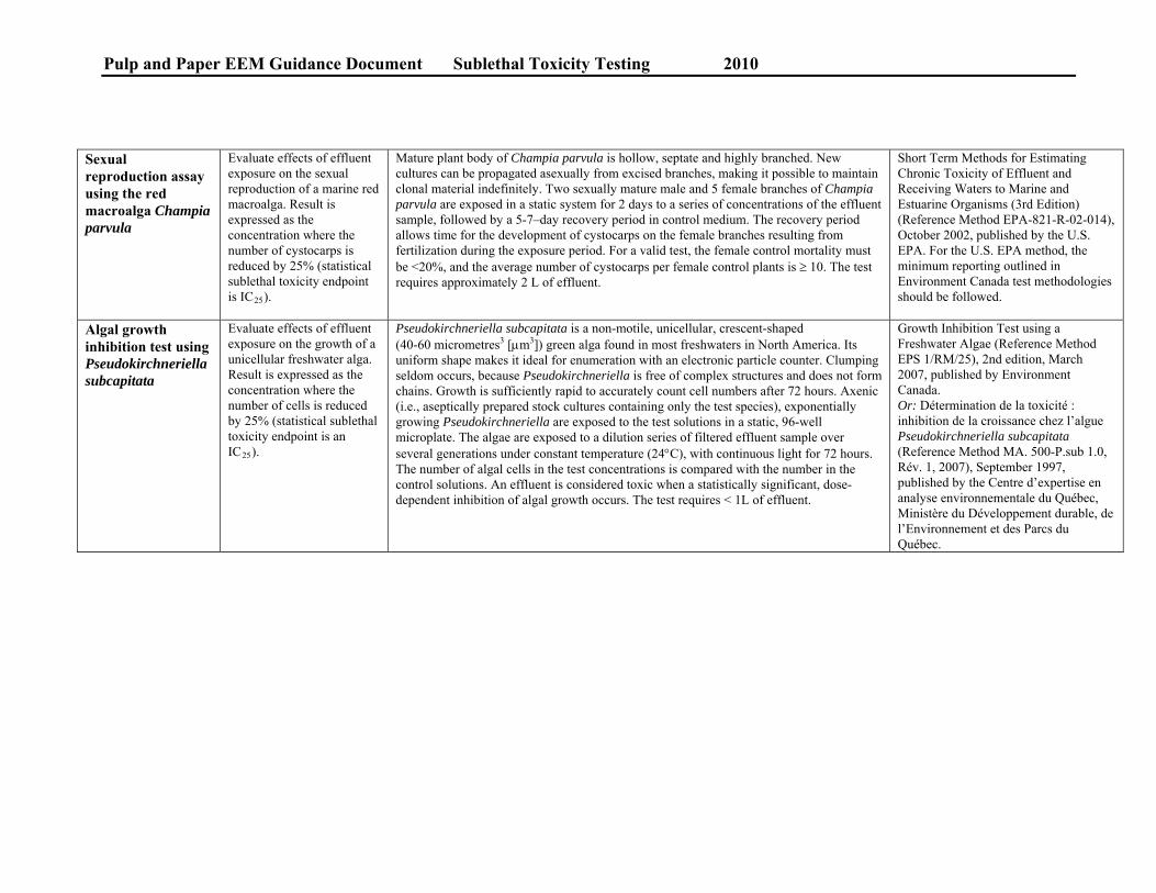
Pulp and Paper EEM Guidance Document Sublethal Toxicity Testing 2010
Sexual reproduction assay using the red macroalga Champia parvula
Evaluate effects of effluent exposure on the sexual reproduction of a marine red macroalga. Result is expressed as the concentration where the number of cystocarps is reduced by 25% (statistical sublethal toxicity endpoint is IC25).
Mature plant body of Champia parvula is hollow, septate and highly branched. New cultures can be propagated asexually from excised branches, making it possible to maintain clonal material indefinitely. Two sexually mature male and 5 female branches of Champia parvula are exposed in a static system for 2 days to a series of concentrations of the effluent sample, followed by a 5-7–day recovery period in control medium. The recovery period allows time for the development of cystocarps on the female branches resulting from fertilization during the exposure period. For a valid test, the female control mortality must be <20%, and the average number of cystocarps per female control plants is 10. The test requires approximately 2 L of effluent.
Short Term Methods for Estimating Chronic Toxicity of Effluent and Receiving Waters to Marine and Estuarine Organisms (3rd Edition) (Reference Method EPA-821-R-02-014), October 2002, published by the U.S. EPA. For the U.S. EPA method, the minimum reporting outlined in Environment Canada test methodologies should be followed.
Algal growth inhibition test using Pseudokirchneriella subcapitata
Evaluate effects of effluent exposure on the growth of a unicellular freshwater alga. Result is expressed as the concentration where the number of cells is reduced by 25% (statistical sublethal toxicity endpoint is an IC25).
Pseudokirchneriella subcapitata is a non-motile, unicellular, crescent-shaped (40-60 micrometres3 [m3]) green alga found in most freshwaters in North America. Its uniform shape makes it ideal for enumeration with an electronic particle counter. Clumping seldom occurs, because Pseudokirchneriella is free of complex structures and does not form chains. Growth is sufficiently rapid to accurately count cell numbers after 72 hours. Axenic (i.e., aseptically prepared stock cultures containing only the test species), exponentially growing Pseudokirchneriella are exposed to the test solutions in a static, 96-well microplate. The algae are exposed to a dilution series of filtered effluent sample over several generations under constant temperature (24C), with continuous light for 72 hours. The number of algal cells in the test concentrations is compared with the number in the control solutions. An effluent is considered toxic when a statistically significant, dose-dependent inhibition of algal growth occurs. The test requires < 1L of effluent.
Growth Inhibition Test using a Freshwater Algae (Reference Method EPS 1/RM/25), 2nd edition, March 2007, published by Environment Canada. Or: Détermination de la toxicité : inhibition de la croissance chez l’algue Pseudokirchneriella subcapitata (Reference Method MA. 500-P.sub 1.0, Rév. 1, 2007), September 1997, published by the Centre d’expertise en analyse environnementale du Québec, Ministère du Développement durable, de l’Environnement et des Parcs du Québec.

Pulp and Paper EEM Guidance Document Sublethal Toxicity Testing 2010
6-10
6.8 Dilution Water in Freshwater Sublethal Toxicity Testing
6.8.1 Dilution Water Selection
The sublethal toxicity test methods required for the pulp and paper EEM program clearly define the culture conditions and test procedures that need to be followed (Environment Canada 1992, 2007a, 2007b; US EPA 1994a, 1994b, 1995, 2002). Some testing decisions are left to the discretion of the individual laboratories, as long as the standard test acceptability criteria can be achieved. For example, standard methods for testing Ceriodaphnia and Pseudokirchneriella allow the use of uncontaminated ground or surface water, dechlorinated tap water or reconstituted water as a source for the culture or the test control/dilution water, as long as the water of choice supports a healthy culture and provides a valid test result.
Most laboratories in Canada use “standard laboratory” water for routine culturing and testing requirements. This water is generally supplied to the laboratory through a natural groundwater system (well) or a local municipal water source, which must be dechlorinated and may be buffered to meet acceptable culturing criteria. Deionized water reconstituted to targeted water quality parameters is also used. Advantages of using laboratory water include the following:
It can be maintained at a consistent quality with minimal risk of contamination by undesirable and/or harmful chemicals or biota.
Regular monitoring of water chemistry and culture health, as well as reference toxicant testing, ensure that the water is of acceptable quality for toxicity testing.
Since cultures are maintained in laboratory water, no additional acclimation is needed for testing effluents or chemicals when laboratory water is used as the control/dilution water.
Laboratory water, normally used in regulatory testing across Canada, provides a measure of the inherent toxicity of the effluents and allows comparison of effluent quality over time.
During the pulp and paper EEM program, most sublethal toxicity tests will likely be performed using laboratory water as control/dilution water, in order to attain comparable results among different laboratories and over time. It is also likely that in many sublethal toxicity tests where there is measurable effluent toxicity, this toxicity can be attributed to inorganic substances such as ammonia, and the toxicity of the effluent may also be affected by site-specific characteristics such as pH, alkalinity and hardness. These characteristics can be controlled and reproduced in the laboratory for cases in which test results, reflective of the site conditions, are desired. However, a mill may decide to test its effluent using unexposed surface water (as control and dilution water), providing the sample is not exposed to effluent. Alternatively, a reference area of similar physicochemical characteristics to a mill site could be used to supply control/dilution water.
The use of unexposed surface waters can be especially helpful in obtaining the following information. Estimating the mitigating or stimulatory effect of unexposed surface site water as dilution water on the expression of toxicity from the effluent discharge or effluent-exposed surface water

Pulp and Paper EEM Guidance Document Sublethal Toxicity Testing 2010
6-11
Although parallel testing of effluents and effluent-exposed surface waters using site water and hardness-adjusted laboratory water have produced similar results (BEAK 1998, 1999), it is impossible to simulate all the physicochemical characteristics of site water using laboratory water. Therefore, if characteristics of site water, other than hardness, alkalinity and pH, are suspected to influence in the expression of toxicity, it may be useful to perform toxicity testing using site water in order to account for site-specific effects.
Unexposed surface water includes mill-site-collected water that has been collected upstream of a mill effluent discharge or from a nearby reference area. Unexposed surface water from the mill site area may vary in physical, chemical and biological characteristics over time.
Disadvantages of using unexposed surface water as dilution/control water include the following:
Relatively large volumes of unexposed surface water may be needed for testing, thus additional expense is incurred for the collection, shipment and storage of site-water samples.
Some laboratory organisms will need acclimation to the unexposed surface water if it is significantly different in physicochemical characteristics from the laboratory water (refer to section 6.9.1).
Mandatory screening of the water through 60-m mesh is required to ensure indigenous populations of micro- or macro-organisms present in surface water do not compete with or impair the health of laboratory test organisms.
In spite of its practical technical disadvantages as control/dilution water, unexposed surface water may provide more site-specific toxicity information. The advantages include the following:
It reflects the physical/chemical characteristics of the receiving environment. It could indicate the potential for non-discharge-related effects. Tests conducted may better reflect the influence of receiving environment characteristics
on toxicant potency than tests conducted with laboratory water.
In Canada, this practice has been logistically constraining due to the large volumes of water needed to be shipped far distances. However, recently it has been shown that individual sites can identify a test organism most likely to detect site-specific changes in effluent quality, so tests using receiving water could be conducted on just 1 species (Taylor et al. 2010). For example, the Pseudokirchneriella test requires smaller volumes of water, making this test an ideal candidate for evaluating the effects of receiving-water chemistry on effluent toxicity (Taylor et al. 2010). Sites should determine which type of water best suits their study objectives.
It should be noted that when using site water, problems may arise with reference water exhibiting sublethal responses. Beak International Inc. (BEAK 1998) attributed this problem to indigenous populations of micro-organisms infecting the laboratory organisms. BEAK staff found that boiling the water prior to use before testing was successful in reducing mortality.

Pulp and Paper EEM Guidance Document Sublethal Toxicity Testing 2010
6-12
Sprague (1997) prepared an extensive review of studies that compared toxicity test results to receiving-water impact, and concluded that effects measured in sublethal toxicity tests correlate with environmental effects most of the time, especially if water collected upstream of the effluent discharge is used as the control/dilution water.
When the purpose of a sublethal toxicity test is to estimate site-specific effects of contaminants, unexposed surface water from the vicinity of the mill site is recommended for use as control/dilution by Environment Canada, the U.S. EPA and the American Society for Testing and Materials (ASTM) in their method and associated guidance documents (Environment Canada 1992, 1998, 2007a; US EPA 1994a; ASTM 1998).
Table 6-3: Specifications of the Environment Canada test methods and recommendations for collection, storage and use of site-collected dilution waters
Criteria Ceriodaphnia dubia Pseudokirchneriella subcapitata
Acceptable Dilution Water For Culturing Uncontaminated groundwater, surface
water, dechlorinated water, reconstituted water, dilute mineral water, or receiving water
Growth medium
For Testing Reconstituted, dechlorinated, uncontaminated groundwater or surface water, receiving water
Reagent water, uncontaminated receiving water, groundwater, surface water or reconstituted water
Site Water Collection Point Upstream from or adjacent to source but
removed from effluent exposure Upstream from or adjacent to source but removed from effluent exposure
Collection Procedure As for effluent As for effluent Acclimation Procedure Recommends acclimating at least 2
generations of brood organisms before collecting neonates for tests
None
Acclimation Rationale Recommended hardness ± 20% of culture water range, alkalinity range ± 20% of culture water
N/A
Treatments Recommend filter 60 µm, boiling if necessary
Filter 0.45 µm
Storage Preferably no more than 14 days; maximum of 1 month at 4ºC with no headspace
Preferably no more than 14 days; maximum of 1 month at 4ºC with no headspace
During Toxicity Testing Include lab water control. If screening test shows impairment, treat water by boiling. If impairment remains, use hardness-adjusted lab water.
Include reagent water control
The widespread acceptance of unexposed surface dilution water for predicting site-specific effects is based on knowledge regarding the interaction of contaminants with water quality characteristics. For example, metal toxicity is well known to be influenced by the physicochemical characteristics of water, such as pH, alkalinity, hardness (reviewed by Wang 1997 and Sprague 1995). However, studies comparing results of toxicity tests on effluents and effluent-exposed surface waters from 4 different mine sites indicated that a similar estimation of toxicity could be obtained from tests using unexposed surface water or laboratory water for dilution, especially if the laboratory water was adjusted to the hardness, alkalinity and pH of the

Pulp and Paper EEM Guidance Document Sublethal Toxicity Testing 2010
6-13
site water (BEAK 1998, 1999). This finding indicates that the use of site-collected dilution water may not always be necessary, because laboratory waters can be prepared to reflect site-water characteristics such as hardness, pH and alkalinity.
Comparing toxicity of the discharge or effluent-exposed surface water relative to an impaired upstream water
If upstream water is contaminated by nonpoint or upstream-point sources of pollution that are unrelated to the mill operation, a mill may decide to use that water for test dilution purposes in toxicity testing in order to provide an appropriate comparison of test organism responses, as long as the upstream water can support the health of the test organisms. If the upstream water cannot support health of the test organisms, it could be tested separately in a dilution series to quantify its effects with uncontaminated reference site or regular laboratory water used for test control and dilutions.
6.9 Collection, Shipment and Storage of Samples for Sublethal Toxicity Testing
The procedures for the collection, shipment and storage of site-collected dilution water are outlined in each of the Environment Canada test methods (Environment Canada 1992, 2007a, 2007b; US EPA 1994a, 1994b, 1995, 2002). Table 6-4 provides estimates of the volumes of site water needed for performing a suite of EEM tests, and includes estimates for effluents or effluent-exposed surface water volume. As recommended by the U.S. EPA (1994a), site-collected dilution water samples should be representative of the water body, unaffected by recent runoff or erosion events that may cause the water to have a higher total suspended solids concentration.
Table 6-4: Dilution/control water and corresponding effluent volumes for sublethal toxicity tests*
Test Dilution Water Volume(L)
Effluent Volume (L)
Ceriodaphnia dubia 10 4Pseudokirchneriella subcapitata 1 1
Testing Series Dilution Water Volume (L)
Effluent Volume (L)
Ceriodaphnia, Pseudokirchneriella 11 5
All volumes are calculated assuming 1 control and 7 test concentrations. * Estimated effluent volumes for marine/estuarine sublethal toxicity tests are outlined in Table 6-2.
Pulp and Paper EEM Guidance Document Sublethal Toxicity Testing 2010
Water Type Reagent Added (mg/L)1 Final Water Quality
6-14
6.9.1 Test Organism Acclimation
Pre-acclimation of culture organisms is recommended prior to exposure to site water. As the purpose of using site water for test control and dilutions is to more accurately predict receiving-water impact, the most accurate prediction should be achieved using organisms adapted to the physicochemical conditions of the receiving environment. The Environment Canada method for Ceriodaphnia dubia recommends that cultures be maintained in water of similar hardness, alkalinity and pH (i.e., within 20%) to the site water used for test dilution (Environment Canada 2007a). BEAK developed a pre-acclimation procedure during the 1997 Aquatic Effects Technology Evaluation (AETE) Program study, later refined in the 1999 study, for Fathead Minnows and Ceriodaphnia dubia (BEAK 1998, 1999). Based on the expected hardness, alkalinity and pH of the site water, cultures are gradually introduced to laboratory water of decreasing hardness over several days until the appropriate hardness is reached. This procedure was adapted from that used by B.A.R. Environmental Inc. (BAR) during its 1996 AETE Program study, in which cultures were gradually acclimated to hardness-adjusted laboratory water and site water if screening of un-acclimated organisms showed impairment to laboratory organisms (BAR 1997).
For pre-acclimation of cultures, laboratory water of reduced hardness may be prepared by diluting standard laboratory water with deionized water. Hardness can be increased by adding salts, used for the preparation of reconstituted water in the appropriate amounts (Table 6-5). When hardness-adjusting water, it is important to keep the alkalinity level appropriate to the hardness, because alkalinity affects the speciation of metals (US EPA 2002; Laurén and McDonald 1986). Appropriate hardness and alkalinity relationships are available in Table 6-5, and additional values may be interpolated (US EPA 1994b).
The detailed procedure for pre-acclimation of Ceriodaphnia dubia is described below. References to hardness assume a corresponding change in alkalinity and pH. No pre-acclimation procedures are described for algal tests as Pseudokirchneriella cultures are maintained in standard culture media that are different from standard testing media.
Table 6-5: Preparation of different hardness/alkalinities
NaHCO3 CaCSO4-2H20 MgSO4 KCL pH2 Hardness3 Alkalinity3
Very soft 12.0 7.5 7.5 0.5 6.4-6.8 10-13 10-13 Soft 48.0 30.0 30.0 2.0 7.2-7.6 40-48 30-35Moderately hard
96.0 60.0 60.0 4.0 7.4-7.8 80-100 60-70
Hard 192.0 120.0 120.0 8.0 7.6-8.0 160-180 110-120Very hard 384.0 240.0 240.0 16.0 8.0-8.4 280-320 225-245
Source: US EPA (1994a) 1 Add reagent-grade chemicals to deionized water. 2 Approximate equilibrium pH after 24 hours of aeration. 3 Expressed as milligrams (mg) CaCO3/L.

Pulp and Paper EEM Guidance Document Sublethal Toxicity Testing 2010
6-15
Ceriodaphnia dubia
Ceriodaphnia cultures are initiated and maintained according to the Environment Canada standard method. To pre-acclimate cultures to the hardness of the site-collected dilution water, a brood of neonates, less than 24 hours old, is initiated in water, reduced in hardness by 20% from that of laboratory water by addition of deionized water. Each day, organisms are transferred to new solutions, decreased by a further 20-30% in hardness. Once the desired hardness is reached (within approximately 1 week) and the culture organisms pass the health criteria of the Environment Canada method (i.e., production of at least three broods, total neonate production of at least 15 per adult, less than 20% adult mortality), a new culture is initiated. The second-generation cultures are maintained in the hardness-adjusted water until organisms pass the health criteria (approximately 1 week). Selenium and vitamin B12 are added to the hardness-adjusted culture water if low in hardness, as recommended by the standard method.
6.9.2 Screening Tests
Once organisms are pre-acclimated to the physicochemical conditions of the site water, they may be exposed to the site water in screening tests. If organisms exposed to the site water meet the test method control acceptability criteria, the site water may be considered suitable for use as dilution water provided the site water meets the control validity criteria for the test method. Comparison of the site-water response to the laboratory response in a screening test may reveal a statistically significant reduction in reproduction and/or survival, even though the site-water-exposed group is within the control acceptability criteria for the test. As long as the site water meets the control validity criteria for the test method, it may be considered suitable for testing. For additional information, consult the Environment Canada test methods.
6.9.2.1 Screening Test Impairment
If organisms are given an adequate opportunity to gradually acclimate to the physical/chemical characteristics of the site water (by exposure to hardness-adjusted laboratory water), impairment observed during screening tests should not be due to shock exposure to different water quality characteristics such as hardness, alkalinity or pH. Therefore, impairment would likely be due to the presence of harmful biological agents or toxicants.
Special attention should be paid to any 100% site-water exposures showing significant mortality in one or more replicates. Microbiological organisms present in the site water may impair the health of test organisms, and anecdotal evidence from several ecotoxicity laboratories indicates that impairment by indigenous micro-organisms usually occurs after a few days of exposure. For example, this has been manifested in Fathead Minnow tests conducted at BEAK as a sudden onset of significant mortality in the site-water control, often in one or two replicates only. Occasionally, evidence of fungal or bacterial growth may be observed in the test vessels. If such contamination is indicated by a screening test, acclimation of the organisms will most likely not result in a removal of impairment. Therefore, either the site water should be treated by a suitable means to remove the impairment (i.e., boiling or ultraviolet treatment—see below), or hardness-adjusted laboratory water should be used as a surrogate.

Pulp and Paper EEM Guidance Document Sublethal Toxicity Testing 2010
6-16
Limited laboratory trials of site water showed that impairment could be removed by boiling site water gently for 10 minutes and cooling it prior to use in testing. Other treatments have been reported in the literature, such as ultraviolet light and 0.45-µm filtration (Grothe and Johnson 1996; Kszos et al. 1997). If site water is collected during late spring to early fall, some form of biological contamination should be expected (unless experience with a particular site water indicates otherwise), and precautions such as boiling should be taken.
If the impairment is due to chemical contamination, the suitability of the site water for use as a dilution and control water is questionable, even though cultures may be acclimated to naturally high levels of metals in site water (see section 6.9.1). If the cultures are exposed to higher levels of contaminants, post-acclimation can result in either higher or lower sensitivity of laboratory organisms, depending on the contaminant, organism and the water characteristics, and the utility of the post–screening test acclimation procedure becomes questionable. If impairment is detected in a screening test, the recommended procedure is to attempt treatment by boiling or to use hardness-adjusted laboratory water as a surrogate dilution water. If it is suspected that site water is contaminated, including a boiled-site-water exposure in screening tests would resolve the question of the effectiveness of that treatment for the site water of interest.
6.9.3 Effluent or Effluent-Exposed Surface Water Toxicity Tests
Table 6-3 summarizes the recommendations for collecting, storing and using site-collected dilution waters in sublethal toxicity testing.
Once site water has been deemed suitable for testing, toxicity tests may be initiated as per the appropriate Environment Canada testing method. In addition to the site-water control, an additional control, using water from the laboratory culture, needs to be included in testing to serve as a check of culture health and site-water quality. No additional control is necessary when the test-control dilution water is the same as the culture water. In the case of Pseudokirchneriella subcapitata tests, the laboratory control would be the standard-test growth medium, specified in the standard method.
If site-collected water is deemed unsuitable for use as test control and dilution water, a treatment such as boiling should be attempted in order to remove the impairment. If successful, the treated site-collected dilution water should be used in testing. If no practical treatment can be found to remove impairment to test organisms caused by the site-collected dilution water, hardness-adjusted water should be used as the dilution water with pre-acclimated organisms. Care should be taken to match the pH of the characteristics of the site-collected dilution water as closely as possible.
6.10 Use of Sublethal Toxicity Testing in Resolving Confounding Influences
Sublethal toxicology data also have the potential utility to aid in the resolution of confounding factors. A multistakeholder group on metal mining toxicology has elaborated on this third use for sublethal toxicity data, and this use is also applicable to the pulp and paper EEM program.

Pulp and Paper EEM Guidance Document Sublethal Toxicity Testing 2010
6-17
Estimating the relative contribution of effluent releases and other natural and/or anthropogenic influences on sublethal toxicity in the same receiving water body
During any phase of the EEM program, sublethal toxicity test data can be used to deal with situations where there are confounding influences. Sometimes the site characteristics do not permit full determination of the mill’s effluent effects even with an adapted study design. Information from sublethal toxicity testing may then help in the interpretation of field results. The choice of when to use sublethal toxicity tests in this application is up to the mill operator and the nature of the confounding influences. However, the confounding influence scenario where sublethal toxicity testing would be most relevant is the multiple-point-source discharge and/or nonpoint-source input situation. Sublethal tests or frequency monitoring should be determined based on the site-specific nature of confounding influence situations.
Estimates of sublethal toxicity can help in understanding the relative contribution of diverse industrial or municipal discharges to effects on aquatic organisms in the receiving water, whether the discharges are from upstream point or nonpoint sources (e.g., municipal landfill leachate, agricultural runoff) or the mill’s property. The upstream contribution of an observed environmental effect can be estimated, given surface water sublethal toxicity data, discharge flow, and features of dispersion into the receiving environment. If plumes from different discharges at a mill site overlap, more effort is necessary to distinguish the toxic contributions of the mill’s discharge sources vs. upstream sources. Samples of surface water from key locations in the near-field exposure areas could be tested, to estimate the combined toxic contribution of the sources.
The following is a 3-step procedure for assessing the relative contribution from different sources of sublethal toxicity to the near-field receiving environment:
Conduct a battery of sublethal toxicity tests on samples collected from all significant discharge sources from the mill’s property. Use standard laboratory water for test dilutions and control, or unexposed site water. This estimates the absolute sublethal toxicity of each mill-site discharge. Repeat the sampling and testing on any discharge that is known to be variable in toxicity, in order to obtain an estimate of the degree of variability.
Conduct a parallel battery of sublethal toxicity tests for each discharge to a river, using water collected directly upstream from the point of discharge for dilution and control. For lakes or estuaries, carry out the parallel battery of tests by collecting control/dilution water from outside the zone immediately affected by the discharges. Separate and simultaneous controls should be run using standard uncontaminated water as a QA measure. It should be recognized that “upstream” sources of control/dilution water might already be contaminated by other effluent discharges or sources of toxicants. Accordingly, the upstream dilution water might contribute to significant effects on growth or reproduction in concentrations of the effluents being studied or even in control vessels. This would not invalidate the results, because the purpose of the investigation is to

Pulp and Paper EEM Guidance Document Sublethal Toxicity Testing 2010
6-18
evaluate the relative contributions of discharges to the total toxicity of the receiving water.
Confirmation of the relative contribution of discharges is recommended, and can be achieved by conducting sublethal toxicity tests on samples of surface water from the water body receiving the discharges (so-called “ambient” tests). This can aid in: a) confirming whether an effluent has a measurable toxicity after mixing into the
receiving water; b) estimating the persistence in the receiving water of toxicity from all contributing
sources; and c) determining the combined toxicity resulting from the mixing of all point and nonpoint
sources, as an estimate of the overall effect on the receiving environment.
Testing samples of surface water, which receives discharges or toxicants from multiple sources, should be done synoptically and ideally during low-flow or worst-case periods. At a minimum, sampling should be carried out over as short a period of time as possible (e.g., 1 or 2 days). Repeated rounds of sampling and testing would be desirable if the toxicity of the discharges were variable. The above guidance on conducting toxicity assessment studies to estimate the contribution of multiple-discharge sources to instream effects is based on the 8 site investigations conducted under the U.S. EPA Complex Effluent Toxicity Testing Program. Detailed reports on these studies were prepared by Mount and Norberg-King (1985, 1986), Mount et al. (1984, 1985, 1986a, 1986b, 1986c) and Norberg-King and Mount (1986).
Mills may elect to conduct additional investigations where the most sensitive species in the effluent produced an IC25 of less than 30%. Below are additional recommended investigations. At a minimum, the most sensitive test species can be used to estimate the geographic extent of the potential response. Alternatively, the results of the toxicity test(s) may lead to or trigger other recommended laboratory or field monitoring tools.
A tiered approach to resolving the confounding influences is recommended, starting with these additional recommended investigations:
1) re-testing with the sublethal test that provided the most sensitive IC25 result, using upstream or reference-site water for test control and dilutions; or
receiving-water toxicity testing with samples collected from the area where a sublethal response is predicted.

Pulp and Paper EEM Guidance Document Sublethal Toxicity Testing 2010
6-19
6.11 References [ASTM] American Society for Testing and Materials. 1998. Standard guide for conducting acute toxicity tests on aqueous ambient samples and effluents with fishes, macroinvertebrates, and amphibians, designation E1192-97. Conshohochen (PA): Annual book of ASTM standards. Section 11: Water and environment technology.
[BAR] B.A.R. Environmental Inc. 1997. Toxicity assessment of mining effluents using upstream or reference site waters and test organism acclimation techniques. Aquatic Effects Technology Evaluation Program. AETE Project 4.1.2a.
[BEAK] Beak International Incorporated. 1998. Additional tool evaluations. Aquatic Effects Technology Evaluation Program. Beak Reference 20776.1.
[BEAK] Beak International Incorporated. 1999. Final report: effects of dilution water on the results of sublethal toxicity tests. Report to Natural Resources Canada. Beak reference 33940.
Chapman PM. 2000. Whole effluent toxicity testing – usefulness, level of protection, and risk assessment. Environ Toxicol Chem 19(1):3-14.
Environment Canada. 1992. Biological test method: fertilization assay with echinoids (sea urchins and sand dollars). Ottawa (ON): Environmental Technology Centre. Report EPS 1/RM/27, December 1992, Amended in November 1997.
Environment Canada. 1998. Biological test method: toxicity tests using the early life stages of salmonid fish (rainbow trout). Report EPS 1/RM/28, 2nd ed., July. Ottawa (ON): Environmental Technology Centre.
Environment Canada. 1999. Recommended procedure for the importation of test organisms for sublethal toxicity testing. Ottawa (ON): Environmental Technology Centre.
Environment Canada. 2001. Revised procedures for adjusting salinity of effluent samples for marine sublethal toxicity testing conducted under environmental effects monitoring (EEM) programs. Ottawa (ON): Method Development and Applications Section, Environmental Technology Centre.
Environment Canada. 2003. National assessment of pulp and paper environmental effects monitoring data: a report synopsis. (NWRI Scientific Assessment Report Series No. 2). Burlington (ON): National Water Research Institute. 28 p.
Environment Canada. 2007a. Biological test method: test of reproduction and survival using the Cladoceran Ceriodaphnia dubia. Ottawa (ON): Environmental Technology Centre. Report EPS 1/RM/21, 2nd edition, February.
Environment Canada 2007b. Biological test method: growth inhibition test using a freshwater alga. Ottawa (ON): Environmental Technology Centre. Report EPS 1/RM/25, 2nd edition, March 2007.

Pulp and Paper EEM Guidance Document Sublethal Toxicity Testing 2010
6-20
[ESG] ESG International Inc. 1999. AETE synthesis report of selected technologies for cost-effective environmental monitoring of mine effluent impacts in Canada. AETE Project 4.1.4, March 1999. Ottawa (ON): Canadian Centre for Mineral and Energy Technology, Natural Resources Canada.
Grothe DR, Johnson DE. 1996. Bacterial interference in whole effluent toxicity tests. Environ Toxicol Chem 15(5):761-764.
Kszos LA, Stewart AJ, Sumner JR. 1997. Evidence that variability in ambient fathead minnow short-term chronic tests is due to pathogenic infection. Environ Toxicol Chem 16(2):351-356.
Laurén DJ, McDonald DG. 1986. Influence of water hardness, pH and alkalinity on the mechanisms of copper toxicity in juvenile rainbow trout, Salmo gairdneri. Can J Fish Aquat Sci 43:1488-1496.
[MDDEP] Ministère du Développement durable, de l’Environnement et des Parcs du Québec. 2007. Détermination de la toxicité : inhibition de la croissance chez l’algue Pseudokirchneriella subcapitata: Centre d’expertise en analyse environnementale du Québec, MA. 500-P.sub 1.0, Revised in September 2007.
Mount DI, Norberg-King TJ, editors. 1985. Validity of effluent and ambient toxicity tests for predicting biological impact, Scippo Creek, Circleville, Ohio. Washington (DC): U.S. Environmental Protection Agency. EPA 600/3-85/044.
Mount DI, Norberg-King TJ, editors. 1986. Validity of effluent and ambient toxicity tests for predicting biological impact, Kanawha River, Charleston, West Virginia. Washington (DC):U.S. Environmental Protection Agency. EPA 600/3-86/006.
Mount DI, Thomas NA, Norberg-King TJ, Barbour MT, Roush TH, Brandes RW. 1984. Effluent and ambient toxicity testing and instream community response on the Ottawa River, Lima, Ohio. Washington (DC): U.S. Environmental Protection Agency. EPA 600/3-84/080.
Mount DI, Steen AE, Norberg-King TJ. 1985. Validity of effluent and ambient toxicity testing for predicting biological impact on Five Mile Creek, Birmingham, Alabama. Washington (DC): U.S. Environmental Protection Agency. EPA 600/8-85/015.
Mount DI, Norberg-King TJ, Steen AE. 1986a. Validity of effluent and ambient toxicity tests for predicting biological impact, Naugatuck River, Waterbury, Connecticut. Washington (DC): U.S. Environmental Protection Agency. EPA 600/8-86/005.
Mount DI, Steen AE, Norberg-King TJ. 1986b. Validity of effluent and ambient toxicity tests for predicting biological impact, Back River, Baltimore Harbor, Maryland. Washington (DC): U.S. Environmental Protection Agency. EPA 600/8-86/001.
Mount DI, Steen AE, Norberg-King TJ. 1986c. Validity of ambient toxicity tests for predicting biological impact, Ohio River near Wheeling, West Virginia. Washington (DC): U.S. Environmental Protection Agency. EPA 600/3-85/071.

Pulp and Paper EEM Guidance Document Sublethal Toxicity Testing 2010
6-21
Norberg-King TJ, Mount DI, editors. 1986. Validity of effluent and ambient toxicity tests for predicting biological impact, Skeleton Creek, Enid, Oklahoma. Washington (DC): U.S. Environmental Protection Agency. EPA 600/8-86/002.
Sprague J. 1995. Factors that modify toxicity. In Rand G, editor. Fundamentals of aquatic toxicology. 2nd edition. Washington (DC): Taylor and Francis.
Sprague J. 1997. Review of methods for sublethal aquatic toxicity tests relevant to the Canadian metal-mining industry. Ottawa (ON): Aquatic Effects Technology Evaluation Program, Canadian Centre for Mineral and Energy Technology, Natural Resources Canada.
Taylor LN, Van der Vliet LA, Scroggins RP. 2010. Sublethal toxicity testing of Canadian metal mining effluents: national trends and site-specific uses. Hum Ecol Risk Assess 16(2):264-281.
[US EPA] United States Environmental Protection Agency. 1994a. Short-term methods for estimating the toxicity of effluents and receiving water to freshwater organisms. Third edition. Cincinnati (OH): Environmental Monitoring Systems Laboratory, U.S. Environmental Protection Agency. EPA /600/4-90/027.
[US EPA] United States Environmental Protection Agency. 1994b. Interim guidance on determination and use of water-effect ratios for metals Office of Water, U.S. Environmental Protection Agency. EPA 823-B-94-001.
[US EPA] United States Environmental Protection Agency. 1995. Short-term methods for estimating the toxicity of effluents and receiving water to West Coast organisms. First edition. Cincinnati (OH): Environmental Monitoring Systems Laboratory, U.S. Environmental Protection Agency. EPA 600/R-95/136.
[US EPA] United States Environmental Protection Agency. 2002. Short-term methods for estimating chronic toxicity of effluent and receiving waters to marine and estuarine organisms. Third edition. Cincinnati (OH): Environmental Monitoring Systems Laboratory, U.S. Environmental Protection Agency. EPA/821/R-02/014, October 2002.
Wang W. 1997. Factors affecting metal toxicity to (and accumulation by) aquatic organisms - an overview. Environ Internat 13:437-457.

Pulp and Paper EEM Guidance Document Data Assessment and Interpretation 2010
7-I
Table of Contents
7. Data Assessment and Interpretation ........................................................................ 7-1
7.1 Overview.......................................................................................................... 7-1
7.2 Understanding the Definition of Effect, and Meaning of Data Interpretation, within EEM.................................................................................................................. 7-2
7.3 Data Assessment and Interpretation for the Fish Study................................... 7-2 7.3.1 Preparing the Analyses ................................................................................ 7-4
7.3.1.1 Immature Fish ...................................................................................... 7-5 7.3.2 Summary Statistics....................................................................................... 7-6 7.3.3 Analysis of Variance (ANOVA) and Analysis of Covariance (ANCOVA) 7-6
7.3.3.1 ANOVA ............................................................................................... 7-7 7.3.3.1.1 Normality and Homogeneity of Variances ...................................... 7-7 7.3.3.1.2 Independence (Pseudo-replication).................................................. 7-8
7.3.3.2 ANCOVA ............................................................................................ 7-8 7.3.3.2.1 Analysis of Residuals..................................................................... 7-10 7.3.3.2.2 Independent Variable ..................................................................... 7-10 7.3.3.2.3 Linear Regression .......................................................................... 7-10 7.3.3.2.4 Slopes of the Regression Lines...................................................... 7-10 7.3.3.2.5 Options for Non-parallel Regression Slopes ................................. 7-11 7.3.3.2.6 Non-parametric Alternatives to ANCOVA ................................... 7-12
7.3.4 Transformations ......................................................................................... 7-13 7.3.5 Level of Replication................................................................................... 7-13 7.3.6 Effect and Supporting Endpoints ............................................................... 7-13
7.3.6.1 Size-at-Age ........................................................................................ 7-13 7.3.6.2 Gonad Weight, Liver Weight, Condition and Fecundity................... 7-14 7.3.6.3 Mean Age........................................................................................... 7-14 7.3.6.4 Age-at-Maturity ................................................................................. 7-14
7.3.7 Statistical Analysis for Non-lethal Sampling............................................. 7-15 7.3.8 Data Quality Assurance / Quality Control and Analysis (Errors and Outliers)7-15
7.4 Effects on Usability of Fisheries Resources .................................................. 7-17 7.4.1 Dioxins and Furans in Fish Tissue............................................................. 7-17
7.4.1.1 Dioxin and Furan Analysis and Reporting ........................................ 7-18 7.4.1.2 Lipid Analysis.................................................................................... 7-18
7.4.2 Physical Abnormalities .............................................................................. 7-19
7.5 Data Assessment and Interpretation for the Benthic Invertebrate Community Study 7-20
7.5.1 Study Design and Statistical Procedures ................................................... 7-20 7.5.2 Data Treatment........................................................................................... 7-22 7.5.3 Reference Condition Approach ................................................................. 7-24 7.5.4 Supporting Endpoints ................................................................................ 7-26
7.6 The Role of Power Analysis, , and Critical Effect Size in Determining
Pulp and Paper EEM Guidance Document Data Assessment and Interpretation 2010
7-II
Effects 7-26 7.6.1 Setting and ........................................................................................... 7-26 7.6.2 Power Analysis: Determination of Required Sample Size, Power and Appropriate Critical Effect Size ............................................................................ 7-29
7.6.2.1 A Priori Power Calculations .............................................................. 7-29 7.6.2.2 Post Hoc Power Analyses .................................................................. 7-31
7.7 Critical Effect Sizes ....................................................................................... 7-32
7.8 Statistical Considerations for Mesocosm Studies.......................................... 7-32
7.9 References...................................................................................................... 7-34
Appendix 1 Step-by-Step Guidance through Statistical Procedures ..................... 7-38
Appendix 2 Graphical and Tabular Representation of Data...................................... 7-58
Appendix 3 Case study – ANCOVA and Power Analysis for Fish Survey ............. 7-75
List of Tables
Table 7-1: Required fish survey measurements, expected precision and summary statistics.................................................................................................................... 7-3
Table 7-2: Fish survey effect indicators and endpoints for various study designs and the appropriate statistical analyses ................................................................................ 7-4
Table 7-3: Supporting endpoints to be used for supporting analyses1............................. 7-4 Table 7-4: Summary of effect endpoints analyzed using ANCOVA .............................. 7-9 Table 7-5: Fish Tissue effect and supporting endpoints and statistical procedure ........ 7-18 Table 7-6: Statistical procedure used to determine an effect for each of the seven study
designs ................................................................................................................... 7-20 Table 7-7: Sample sizes required to detect difference of ± 2 SD .................................. 7-28

Pulp and Paper EEM Guidance Document Data Assessment and Interpretation 2010
7-1
7. Data Assessment and Interpretation
7.1 Overview
As part of the environmental effects monitoring (EEM) requirements under the Pulp and Paper Effluent Regulations (PPER), after biological monitoring studies are conducted, an interpretive report shall be prepared (PPER, Schedule IV.1, section [s.] 12). The owner or operator shall submit to the Authorization Officer reports of the results of the studies in writing and the supporting data in the electronic format provided by Environment Canada. The role of the interpretive report within the EEM program is to summarize study results (including difficulties or confounding factors encountered), conduct applicable spatial analyses (and when sufficient data are available, temporal trend analyses), specify any identified “effects,” and make recommendations for subsequent EEM program monitoring. Data interpretation or the role of the report does not include determining the ecological, economic or social significance of results. The content of the interpretive report is available in Chapter 9 of this document and in the PPER.
The purpose of this chapter is to provide general guidance on how to assess and interpret EEM data, specifically:
1) which effect endpoints to use and report; 2) the statistical (or other) approach to use for each effect endpoint in order to determine the
presence or absence of an effect; and 3) the role of power analysis, , and critical effect size (CES) in determining effects.
Further guidance on these issues can be found in supplementary documents available via the EEM website (www.ec.gc.ca/eem).
EEM involves iterative cycles of monitoring and reporting. For each cycle it is required to report the results of the data assessment made under Schedule IV.1, s. 11. The report must include the identification of any effects on fish populations, fish tissue or the benthic invertebrate community, the overall conclusions of the biological monitoring studies based on the results of the statistical analysis, and a summary of the results of previous monitoring. More specifically, the data generated for each mill should be analyzed to determine whether there are significant differences in certain effect indicators between reference and exposure areas or along an exposure gradient (i.e., determination of effect). In addition to the within-cycle (spatial) analysis, a comparison of effects between cycles (temporal comparisons) is recommended in order to determine whether any effects identified previously are lessening or worsening.
For EEM purposes, only specified data (the effect indicators) generated from the fish survey, benthic invertebrate community survey and fish usability studies are used to assess the presence of effects. Other EEM data are only used to help interpret effects on fish and benthos (e.g., effluent characterization and water quality monitoring) or to help characterize any changes in effluent quality over time (e.g., sublethal toxicity testing). The tables in the

Pulp and Paper EEM Guidance Document Data Assessment and Interpretation 2010
7-2
following sections summarize the recommended data analysis procedures for the effect indicators for each monitoring requirement (tables 7-2, 7-3 and section 7.5). Also, refer to the relevant sections of this chapter for further details. Many of the data interpretation issues are the same for the fish survey, fish usability and benthic invertebrate community sections that follow (e.g., assumptions and interpretation of statistical techniques common to more than one of these sections). Several of these common issues are discussed in the fish section below, and are not repeated in the following sections on fish usability and benthic invertebrate communities.
7.2 Understanding the Definition of Effect, and Meaning of Data Interpretation, within EEM
Understanding 1) the types of data analyses that are relevant and 2) what is meant by the definition of “interpretation” is integral to the EEM program, particularly when writing an interpretation report. In order to address both issues, it is important to define “effect.”
Within EEM, an effect is defined generally as a statistically significant difference in fish, fish usability or benthic invertebrate community effect indicators measured between an area exposed to effluent and a reference area, or a statistically significant difference in these effect indicators within an exposure area along a gradient of effluent concentrations. For fish tissue analysis (which is conducted to determine the usability of fisheries resources), an effect is defined when the concentration of dioxins and furans, expressed as toxic equivalents of 2,3,7,8-tetrachlorodibenzo-para-dioxin, exceeds 15 picograms per gram (pg/g) wet weight in muscle or 30 pg/g wet weight in liver or hepatopancreas in fish taken in the exposure area (PPER Schedule IV.1, s. 1). In cases where it is not feasible to examine wild fish or field distribution of benthic invertebrates in areas exposed to effluent and reference areas, an alternative monitoring approach for fish or fish habitat may be used to determine if the effluent is causing an effect.
Given the above definition of effect, it is important to recognize that not all effects identified in EEM represent damage to fish, fish habitat or the usability of fisheries resources. However, effects as defined above do represent scientifically defensible differences or gradients that may reflect changes to the ecosystem associated with the effluent. As a result, detailed information on the effects, including the magnitude, geographic extent and possible cause of the effect, may contribute to the understanding of the ecosystem and could be used in the management of the aquatic resources.
7.3 Data Assessment and Interpretation for the Fish Study
The data collected during the fish population study will include indicators of growth, reproduction, condition and survival (when it is possible to obtain data to establish the indicators), that include the length, total body weight and age of the fish, the weight of its liver or hepatopancreas, and, if the fish are sexually mature, the egg weight, fecundity and gonad weight of the fish (PPER Schedule IV.1, s. 11).

Pulp and Paper EEM Guidance Document Data Assessment and Interpretation 2010
7-3
The overall procedure that should be followed and reported can be divided into the following stages: 1) preparing the analyses, 2) initial summary statistics, 3) analysis of variance (ANOVA) analyses, 4) analysis of covariance (ANCOVA) analyses, and 5) power analyses. Appendix 1 provides a step-by step-guidance through the statistical procedures for the fish survey.
The required fish survey measurements, expected precision, and summary statistics are described in Table 7-1. Table 7-2 outlines the effect indicators for various study designs and the appropriate statistical analyses that are applicable for the fish population study. Table 7-3 outlines the supporting endpoints.
Table 7-1: Required fish survey measurements, expected precision and summary statistics
Measurement Requirement (PPER Schedule IV.1, subparagraphs [subpars.] 11(a)(i) and (b))
Expected Precision*** Reporting of Summary Statistics (PPER Schedule IV.1, s. 11) and other general reporting
Length (fork or total or standard)* +/- 1 millimetres (mm) Mean, standard deviation (SD), standard error, minimum and maximum values for sampling areas
Total body weight (fresh) +/- 1.0% Mean, SD, standard error (SE), minimum and maximum values for sampling areas
Age +/- 1 year (10% to be independently confirmed)
Mean, SD, SE, minimum and maximum values for sampling areas
Gonad weight (if fish are sexually mature)
+/- 0.1 grams (g) for large-bodied fish species and 0.001 g for small-bodied fish species
Mean, SD, SE, minimum and maximum values for sampling areas
Egg size(if fish are sexually mature)
+/- 0.001 g Weight, (recommended minimum sub-sample sizes of 100 eggs), mean, SE, minimum and maximum values for sampling areas
Fecundity** (if fish are sexually mature)
+/- 1.0% Total number of eggs per female, SE, minimum and maximum values for sampling areas
Weight of liver or hepatopancreas +/- 0.1 g for large-bodied fish species and 0.001 g for small-bodied fish species
Mean, SD, standard error, minimum and maximum values for sampling areas
External condition n/a Presence of any lesions, tumours, parasites or other abnormalities
Sex n/a
* If caudal fin forked, use fork length(from the anterior-most part to the fork of the tail). Otherwise, use total

Pulp and Paper EEM Guidance Document Data Assessment and Interpretation 2010
Effect Endpoint and Statistical Procedure
7-4
length, and report type of length measurement conducted for each species. In cases where fin erosion is prevalent, standard length should be used.
** Fecundity can be calculated by dividing total ovary weight by weight of individual eggs. Individual egg weight can be estimated by counting the number of eggs in a sub-sample. The sub-sample should contain at least 100 eggs.
*** For small-size fish weights, use at least a 3-decimal scale.
Table 7-2: Fish survey effect indicators and endpoints for various study designs and the appropriate statistical analyses
Effect Indicator Standard Survey Non-lethal Sampling Wild Molluscs
Growth (EnergyUse)
Size at age (body weight against age) (ANCOVA)
Size (length and weight) of young of the year (age 0+) at end of growth period (ANOVA)
Whole-animal wet weight (ANOVA)
Reproduction (Energy Use)
Relative gonad size (gonad weight against body weight) (ANCOVA)
Relative gonad size (gonad weight against body weight) (ANCOVA)
Condition (Energy Storage)
Body weight relative to length Relative liver weight (liver weight against body weight) (ANCOVA)
Body weight relative to length (ANCOVA)
Whole-animal dry weight, dry shell or soft tissue weight related to shell length (ANCOVA)
Survival Age (ANOVA) Length frequency distribution (2-sample Kolmogorov-Smirnov test)
Length frequency analysis (2-sample Kolmogorov-Smirnov test)
Table 7-3: Supporting endpoints to be used for supporting analyses1. Effect Indicator
Supporting Endpoint Statistical Procedure
Energy Use Body weight (whole) ANOVA Length ANOVASize-at-age (length against age) ANCOVA Relative gonad size (gonad weight against length) ANCOVA Relative fecundity (# of eggs/female against body weight) ANCOVA Relative fecundity (# of eggs/female against length) ANCOVA Relative fecundity (# of eggs/female against age) ANCOVA
Energy Storage Relative liver size (liver weight against length) ANCOVA Relative egg size (mean egg weight against body weight) ANCOVA Relative egg size (mean egg weight against age) ANCOVA
Note: these analyses are for informational purposes, and significant differences between exposure and reference areas are not necessarily used to designate an effect.
1 For the ANCOVA analyses, the first term in parentheses is the endpoint (dependent variable, Y) that is analyzed for an effluent effect. The second term in parentheses is the covariate, X (age, weight or length).
7.3.1 Preparing the Analyses

Pulp and Paper EEM Guidance Document Data Assessment and Interpretation 2010
7-5
Upon completion of the field and laboratory measurements, the data should be promptly entered into a computer spreadsheet and quality assurance / quality control (QA/QC) should be conducted. Values entered into the spreadsheet should be double-checked with the original handwritten data sheet to prevent typographical errors. A data matrix with the location identifier (area), variables in columns, and observations in rows operates as the fundamental working unit. In this spreadsheet, include a column for comments on the physical condition and any abnormalities noticed during the sampling process. These comments may prove to be useful in identifying unusual observations and help to determine whether data should be removed from an analysis. A location identifier for area or site should be chosen—one that can be easily distinguished as reference or exposure. This will allow for easier interpretation for others who are not familiar with the location identifier codes. If an insufficient number of fish were collected at an exposure site but were collected at the reference site, be sure to make special note of this.
Failure to identify transcription errors can invalidate further analyses. Assuming the data have been entered correctly, data that will be necessary for interpretation should be summarized, screened for erroneous values and outliers, and assessed for normality and transformed if necessary; and, any significant confounding factors should be summarized.
Differences between sexes in growth rate, body weight, condition factor, gonad size and liver size are common, due to differences in overall energetic requirements between male and female fish. Therefore, for all parameters, sexes should initially be treated separately when conducting the analyses. In addition, sexually immature fish should not be mixed with sexually mature fish for analyses.
7.3.1.1 Immature Fish
It should be confirmed that all fish which are assumed to be adults are undergoing gonadal development for the next spawning season. The inclusion of immature fish into statistical analyses can provide misleading results. Immature fish devote proportionally more energy toward growth, so the body size-gonad relationship for immature fish is different than that of adult fish. For data analysis, fish identified as immature in the spreadsheet should be removed. The gonadosomatic index (GSI) = gonad weight / body weight x 100 can be useful in identifying immature fish. As a general rule, for many fish species, immature fish can be categorized as having a GSI of < 1%, although there are some notable exceptions, such as guarding species like the Brown Bullhead. A plot of gonad weight vs. body weight, and using this general rule for GSI, can be most useful in identifying immature fish. Comments from the field observations may also assist in identifying unusual observations that are suspected to be immature (e.g., comments such as “weighed only one testis”). The sampling period has to be adjusted to the biology (life history) of the species to avoid capturing fish prior to gonadal development for the upcoming reproductive season. However, when non-lethal sampling is to be carried out and age-frequency distributions are used to assess reproductive success, the timing of sampling is less important. Data analysis on immature and mature fish should be conducted separately, except, for obvious reasons, when comparing the proportion of non-spawning fish among sites.

Pulp and Paper EEM Guidance Document Data Assessment and Interpretation 2010
7-6
7.3.2 Summary Statistics
The descriptive statistics (mean, standard deviation [SD], standard error [SE]) and the minimum and maximum values will be determined, when it is possible to obtain data, to establish the indicators of growth, reproduction, condition and survival that include the length, total body weight and age of the fish, the weight of its liver or hepatopancreas, and, if the fish are sexually mature, the egg weight, fecundity and gonad weight of the fish (PPER Schedule IV.1, s. 11). The fish survey measurements to determine effects in fish growth, reproduction, condition and survival, the expected precision, and summary statistics are described in Chapter 3.
The summary statistics should be calculated by species and sex for each area being summarized (e.g., reference area and exposure area). Before calculating summary statistics, the data should be graphed using box plots for examination of extreme outliers. The summary statistics should be presented in graphical and tabular format for all variables. The data should be examined for normality and equality of variances (basic statistical assumptions). Note that slopes and adjusted means and associated error terms should also be reported for ANCOVA, as outlined below.
Visual screening techniques such as box and whisker plots, normal probability plots, and stem-and-leaf diagrams can be used to identify extreme values (true outliers and/or data entry errors). Most statistical software packages provide data summary modules capable of generating appropriate summary statistics and graphics.These summary statistics are usually needed for presentation, and aberrantly high or low values can indicate errors. Extreme values or outliers should not be removed from the data set (unless they are obvious sampling, measurement or data entry errors) (Grubbs 1969; Green 1979), because mistakenly removing valid data will result in the loss of statistical power in the fish survey. Instead, extreme values should be identified in the report and the influence of the extreme value(s) on the results should be determined by reanalyzing the data without the extreme value.
7.3.3 Analysis of Variance (ANOVA) and Analysis of Covariance (ANCOVA)
In addition to descriptive statistics, an analysis of the results must be conducted to determine if there is a statistical difference between the sampling areas (PPER Schedule IV.1, paragraph [par.] 11(c)). This is usually conducted using ANOVA or ANCOVA. However, in some instances, other statistical procedures (e.g., non-parametric methods) may be used. The analyses (for ANOVA and ANCOVA) that are used to determine whether statistically significant effects have occurred should follow these three steps of data inspection, analysis and interpretation (Appendix 1 provides a step-by-step guidance through the statistical procedures for the fish survey):
1) The data should be inspected to see whether they satisfy the assumptions of ANOVA or ANCOVA. These procedures are robust enough to allow for moderate violations of some assumptions and, in some cases, data transformation will help to remedy departures from

Pulp and Paper EEM Guidance Document Data Assessment and Interpretation 2010
7-7
the assumptions. In cases where data transformations do not sufficiently rectify departures from the assumptions, it may be necessary to use non-parametric procedures, in which case the methods of power analysis discussed in section 7.6 would not apply. These issues are further discussed below, and the standard statistical texts (e.g., Sokal and Rohlf 1995) should be consulted for a more complete discussion.
2) Following inspection of the data and any necessary transformations, the actual statistical comparisons are carried out.
3) After the statistical comparisons are made, key results for the effect indicators (Table 7-1) should be presented in a clear fashion so as to indicate whether there has been effects and, if so, the nature of the effects (including the direction and magnitude of the effects). An effect is declared if the p-value is less than the a priori value determined, as outlined in section 7.6.
7.3.3.1 ANOVA
ANOVA is used to test for site differences in length, weight and age. The assumptions for ANOVA are that:
the data for reference and exposure populations are normally distributed; the variances are equal between the reference and exposure populations; and the error terms are independently distributed.
A one-factor ANOVA is used to test for differences in the mean response (length, weight or age) using the factor site (e.g., reference or exposure). A residual plot can be useful in identifying outliers. Observations with studentized residuals with a magnitude greater than 4 typically warrant investigation. Non-parametric alternatives for ANOVA include the Kruskal-Wallis test, or, if comparing two sites, the Mann-Whitney test (non-parametric alternative to the two-sample T-test).
7.3.3.1.1 Normality and Homogeneity of Variances
The assumptions of normality and homogeneity of variance should be assessed before applying most parametric procedures. However, most univariate normal distribution-based statistical methods are quite robust and can support moderate violations of the assumptions. Transformation of original data will help normalize the data or homogenize the variances. Logarithmic transformations are often preferred because most biological measures are considered to operate on a log or exponential scale (Peters 1983) and such a transformation is biologically meaningful. It should be noted that for the purposes of the fish EEM survey, 1 should not be added to values before logging because it has undesirable effects on the calculated variances when changing measurement units. If the transformations are unable to produce data that meet the assumptions, a plot of the residuals may reveal problematic data points that may warrant investigation. Most of the univariate statistical methods are robust under moderate violations of assumptions, with some exceptions such as analyses with small

Pulp and Paper EEM Guidance Document Data Assessment and Interpretation 2010
7-8
and unequal samples. For serious violations, non-parametric statistics can be considered.
7.3.3.1.2 Independence (Pseudo-replication)
When designing experiments, it is desirable to ensure that replicates are randomly allocated to different treatment levels, such that the responses of each replicate are independent of other replicates. This element of randomness provides some assurance that observed differences in responses among treatments results from treatment effects and not from other factors.
Lack of independence can occur when, for example, one person collects all the data from the exposure area while another person collects data from the reference area. This can bias the data if the two individuals consistently use slightly different sampling or sorting protocols. Generally, these kinds of problems can only be remedied by changing the method of conducting the sampling so as to remove the sources of bias.
Randomly allocating replicates to different treatment levels is a relatively easy procedure when conducting manipulative experiments (e.g., controlled laboratory tests), but is less obvious for observational field studies. Observational studies, such as environmental impact studies (e.g., single-stressor EEM studies) or environmental assessments (i.e., multiple stressors), test hypotheses about the presence and magnitude of effects. However, the strength of inferences from these types of experiments is limited, for two reasons (Paine et al. 1998):
the stressor (e.g., mill outfall, hydroelectric dam) cannot be reproduced; and stressors cannot be applied randomly to replicates.
What this means is that the stressor or treatment is always partly or wholly confounded with space or time, and that the observed effects may or may not be caused by the stressor of interest. For example, when investigating whether effluent from an industrial plant is having an effect on downstream fish populations, it is not possible to replicate the treatment of effluent exposure (i.e., there is only one plant and outfall), or to randomly assign fish populations to the different treatment levels (reference vs. exposed). As such, when significant differences are observed between reference and exposed fish populations, one can conclude that there are differences between these two populations, but not necessarily that the differences were caused by effluent exposure. Interpreting significant differences as treatment effects when either treatment is not replicated or replicates are not independent is referred to as pseudo-replication (Hurlbert 1984).
Before attributing cause to any specific stressor, it is critical that observations be confirmed, through replication over time, and that some effort be expended to confirm that the stressors of interest are involved in the responses.
7.3.3.2 ANCOVA
ANCOVA is used to test for site differences in condition, relative gonad weight, relative

Pulp and Paper EEM Guidance Document Data Assessment and Interpretation 2010
7-9
liver weight, weight-at-age, size-at-age, and relative fecundity. A summary of these analyses is provided below.
Table 7-4: Summary of effect endpoints analyzed using ANCOVA Effect Endpoint Response Variable Covariate Condition Body weight LengthRelative liver weight Liver weight Body weight Relative gonad weight Gonad weight Body weight Weight-at-age Body weight Age Size-at-age Length Age Relative fecundity Eggs/female Body weight
The assumptions for ANCOVA are that:
the relationship between the response and covariate is linear; the slopes of regression lines among sites are parallel; the covariate is fixed and measured without error; and the residuals are normally and independently distributed with zero mean and a
common variance.
It should be noted that ANCOVA is basically a two-step procedure consisting of:
a) determining whether the slopes are approximately parallel; and b) if the slopes are parallel, going on to determine whether the elevations of the
regressions are significantly different. This procedure is discussed more fully below.
ANCOVA is used to test for differences in a response among sites while taking into account the variability in test subjects by including a covariate in the analysis. This inclusion of a covariate in the analysis decreases the error term (by accounting for the variability explained by the regression of the response variable on the covariate) and thus increases the power of the test (Huitema 1980).
It has been suggested that the range of the independent variable (covariate) should be approximately the same for each site. This will be difficult to assure in practice, but the violation of this should be considered when interpreting results from such cases. If there is reason to believe that there are issues with the overlap of the range of covariate values, perform a single-factor ANOVA on the covariate values between sites. If the covariate means do not significantly differ between sites, the results of the ANCOVA will probably be reliable (Quinn and Keough 2002). A significant difference in the mean covariate values between sites is a significant effect. In interpreting differences in the covariate means or ranges observed, take into consideration the consistency of sampling gear between sampling sites and the selection of samples. It may be appropriate to provide an analysis of a subset of the data, omitting unusually high or low covariate values in order to provide a reliable analysis.
The range of covariate values for the weight-at-age effect endpoint must be considered

Pulp and Paper EEM Guidance Document Data Assessment and Interpretation 2010
7-10
before performing an ANCOVA. For several small-bodied fish species, the range of the covariate (age) might only be between 2 and 3 or 2 and 4. An ANCOVA with only 2 or 3 values of the covariate can provide misleading results. In these cases it may be appropriate to perform a one-factor ANOVA on body weight, using site as the factor for each age group.
7.3.3.2.1 Analysis of Residuals
The preferred method of examining the residuals is to use graphical methods rather than relying on formal tests to assess normality and equality of variance. In fact, Day and Quinn (1989) have recommended against using formal tests. A good discussion of this topic can be found in Miller (1986). Draper and Smith (1981) review various methods of examining residuals, particularly residuals from regressions. Most statistical software packages also provide modules for examination of residuals. These methods are usually graphical, although diagnostic statistics are available as well. The primary advantage of these methods, compared to formal tests, is that they can identify the cause of violations of normality or equality of variances.
7.3.3.2.2 Independent Variable
The assumption that the independent variable is fixed is frequently violated, and Draper and Smith (1981) discuss the consequences of this violation. A non-fixed independent variable is likely to prove problematic, mainly in situations where the range of the independent variable is very small, i.e., when the range in size (or age) of the fish included in the regression is very small. In this case (very narrow size or age range), there is little to be gained by using ANCOVA with size or age as a covariate, and the data would be better analyzed as a simple ANOVA comparison of the exposure to reference area (i.e., no need to factor out the influence of the covariate).
7.3.3.2.3 Linear Regression
The assumption of a linear relationship can be tested for samples with multiple observations at different values of the independent variable. This may be possible for discrete variables such as age, but not for continuous independent variables such as body weight. At a minimum, linearity should be verified by visual inspection. Linearity can often be improved by transformation (e.g., the log-log transformation is used very widely for this purpose for the EEM fish ANCOVA analyses). The regression plots should also be inspected to ensure that the slopes are not unduly influenced by outliers. Scatter plots help identify outliers and unusual data. For example, when reproductive data are analyzed for fish, the plots aid in identifying potential “immature” fish that could affect the results. The scatter plots should be included in the interpretive report.
7.3.3.2.4 Slopes of the Regression Lines
A key assumption of ANCOVA is that the slopes of the regression lines for the reference vs. exposure areas are approximately equal. Therefore, the first part of an ANCOVA analysis is to test for differences in slopes between areas. A significant interaction term in the

Pulp and Paper EEM Guidance Document Data Assessment and Interpretation 2010
7-11
ANCOVA for covariate X vs. area (e.g., age*area or size*area) indicates significantly different slopes. In cases where the slopes are not significantly different (i.e., interaction term not significant), this indicates that the regression lines are approximately parallel to each other. Using the weight-at-age ANCOVA as an example, parallel slopes would indicate that weight gain over age is similar for both areas. The next step in this example is to proceed with the ANCOVA model, and test for differences in adjusted means (elevation) to investigate whether fish are proportionately heavier at any age in one area than in another.
It is possible that the slopes of regressions may differ. For example, fish from the reference area may be gaining weight more rapidly with increasing age (steeper slope) than fish from the exposure area. If the slopes of the regressions are significantly different, the ANCOVA cannot be completed. In this case, using the weight-at-age example, the effect would not be a proportional difference in weight at any age; rather, the rate of weight gain with increasing age would be significantly different among areas. This is considered a statistically significant EEM effect for the fish survey. That is, an effect would be determined as a significant difference in slope among areas rather than a significant difference in elevation. For this situation, it is also a good idea to plot separate regression lines to obtain a better qualitative understanding of the weight-at-age relationship for each area over the entire data range of the X covariate (e.g., where do the lines intersect?). It should be noted that, even when the slopes of the regressions significantly differ among areas, it is still possible to make further comparisons over a particular range of values for the X covariate (i.e., a particular age or size range) (Sokal and Rohlf 1995). This kind of comparison would be appropriate if it is judged that that particular age or size range is of particular concern.
It is also preferable that the range of the independent variable be approximately the same for each “treatment” (i.e., area). This may be difficult to assure in practice, but any violation of this should be considered when interpreting results from such cases. For example, if the size range used as the X covariate for the reference area does not show much overlap with the size range for the exposure area, use of the ANCOVA results requires the assumption that the regression slopes would still be parallel for overlapping size ranges and may not be appropriate in this situation.
7.3.3.2.5 Options for Non-parallel Regression Slopes
When the assumption of parallel regression slopes is not met, ANCOVA cannot proceed, because adjusted treatment means cannot be correctly interpreted. In this case there is a covariate by treatment interaction, and differences in the response variable among treatments vary at different values of the covariate. There are a few options for dealing with non-parallel regression slopes in ANCOVA. These are discussed below in the order that the methods should be applied to data sets with non-parallel slopes. The first two options provide mechanisms by which the slopes can be treated as being parallel, thus allowing a full ANCOVA and comparison of adjusted means. The third option provides an alternative methodology for calculating measured effects when the slopes cannot be treated as being parallel, even after applying options 1 and 2.
1. Influential Points (from Barrett et al. 2010)

Pulp and Paper EEM Guidance Document Data Assessment and Interpretation 2010
7-12
Influential points are observations with high leverage (outliers in the covariate space) that have the potential to dominate conclusions by producing substantial influence on the regression coefficients (Fox 1997). If one or more points is highly influencing the slope of a regression line and causing non-parallel slopes, removal of this (these) point(s) may remove the evidence against fitting the data to the parallel model. Influence can be assessed using the Cook’s distance statistic (Cook 1977, 1979), which is incorporated into many statistical software packages. It is calculated using studentized residuals (outliers in the response variable) and a measure of leverage called “hat values” (outliers in the predictor variable) as a measure of impact for each observation (Fox 1997). A plot of Cook’s distance vs. the covariate is most useful in identifying high-influence observations. A numerical cut-off of 4 / (n-k-1), where n is the total number of observations and k is the number of predictors in the regression model, can also be used to assess high-influence observations (Fox 1997).
2. Coefficients of Determination (from Barrett et al. 2010)
The coefficient of determination (R2) expresses the proportion of the total variability in the response variable that is explained by its linear relationship with the independent variable, and is a measure of the association between the two variables (Quinn and Keough 2002). When the regression slopes are found to be non-parallel, the R2 of the full regression model (model with the interaction term included) can be compared to the R2 of the reduced regression model (model with the interaction term removed). When the R2 of the parallel (reduced) model is high (greater then 0.8) and only slightly (less than 0.02) lower than that of the full model, the parallel model can provide a sufficient representation of the data and can be used to proceed with the analysis.
3. Estimating Effects for Different-sized Fish (from Lowell and Kilgour 2008)
When the above two methods cannot be applied to the data set (i.e., when the slopes remain non-parallel even after applying the above two methods), the following method can be used to estimate measured effects for smaller (or younger) and larger (or older) fish. First determine the minimum and maximum values of the covariate within the range of covariate overlap for the two regressions (reference and exposure areas). Then, determine the predicted values of the response variable for each area regression line at these two covariate values (minimum and maximum). An estimate for the effect at the minimum covariate value (i.e., the effect on smaller or younger fish) will be the difference in predicted values, calculated as exposure-predicted value minus reference-predicted value, expressed as a percentage of the reference-predicted value. If the data were log-transformed, the predicted values must be anti-logged (i.e., x expressed as 10x) before calculating the percent difference. The calculation is the same for larger (or older) fish, but using the maximum value of the covariate where the ranges for each area overlap. Each of these two measured effects (percent differences for small/young fish and large/old fish) can then be compared to CESs in the same way as is done for measured effects calculated from means (from ANOVA) or adjusted means (from ANCOVA).
7.3.3.2.6 Non-parametric Alternatives to ANCOVA

Pulp and Paper EEM Guidance Document Data Assessment and Interpretation 2010
7-13
ANCOVA is robust to violations of the assumptions of the test when sample sizes are approximately equal (Huitema 1980; Hamilton 1977). When assumptions are seriously violated and sample sizes are unequal, non-parametric alternatives to ANCOVA could be considered. Several different non-parametric techniques using ranks have been proposed. Iman and Conover (1982) proposed a non-parametric alternative in which the response and covariate are replaced by their ranks. The analysis is the same as the parametric ANCOVA using the ranks as data, and is the simplest non-parametric alternative. Groups of tied ranks are replaced by the average rank for that grouping. Some other non-parametric alternatives are discussed in Shirley (1981) and Quade (1967).
7.3.4 Transformations
Transformations of the data can often help improve normality and homogenize variances (reduce some violations), and an examination of the relationship between the means and variances can help identify the most appropriate transformation (see Green 1979). Taylor’s Power Law (Taylor 1961), which examines the relationship between treatment means and variances, can be used to determine the specific transformations in order to normalize data or homogenize variances (Green 1979). Logarithmic transformations are often preferred because biological measures are frequently considered to operate on a logarithmic or exponential scale (Peters 1983). It should be noted that 1 should not be added to values before logging for the purposes of the fish EEM survey, because it has undesirable effects on the calculated variances when changing measurement units. If the transformations are unable to produce data that approximately meet the assumptions, it may be necessary to use non-parametric statistics.
7.3.5 Level of Replication
For each of the ANOVA and ANCOVA analyses, the level of replication (sample size, n) is the number of individual fish. The minimum sample size recommended is 20 sexually mature fish per sex (and an additional 20 sexually immature fish if small-bodied fish species are being sampled) for each of the 2 sentinel fish species in both the reference and exposure area. A power analysis should be conducted to determine sample size if the appropriate data are available.
7.3.6 Effect and Supporting Endpoints
7.3.6.1 Size-at-Age
Rates of growth are commonly described by the relationship of size (as weight or length) to age. Over the entire lifespan of a fish, this relationship is curvilinear, with the rate of increase declining as fish approach the limit of their lifespan (Ricker 1975).As only adult fish are often sampled, classical growth rates cannot be calculated. Nevertheless, for the purposes of the EEM program, fish growth can be inferred from size-at-age estimates determined for each area using ANCOVA. This calculation assumes that the relationship

Pulp and Paper EEM Guidance Document Data Assessment and Interpretation 2010
7-14
between size and age for adult fish is approximately log-linear (log size vs. log age) (Bartlett et al. 1984).
Size-at-age may be estimated by calculating the regression relationship between body size (weight or length) and age for each sampling area (reference and exposure). It is recommended that both length and weight be used to calculate size-at-age, in order to determine which provides the best fit and tightest regression.
7.3.6.2 Gonad Weight, Liver Weight, Condition and Fecundity
Relative gonad and liver size (and fecundity) are obtained by regression and analyzed using ANCOVA, using body weight as the covariate. Likewise, condition is obtained by regressing body weight against body length, and essentially describes how “fat” fish are at each area.
A variety of indices have been used in fisheries biology to describe the condition of fish (Bolger and Connolly 1989). Calculating the ratio of one variable to another has been used to derive many of them. Examples of a few common indices are):
condition factor (k) = 100 (body weight/length3); GSI = 100 (gonad weight/body weight); and liver somatic index (LSI) = 100 (liver weight / body weight).
In general, however, investigators have become cautious about using derived variables and ratios because they may have undesirable statistical properties (Green 1979; Jackson et al. 1990). Although these indices may be used for presentation purposes, it is preferable statistically to estimate (and analyze) the parameters from regressions of original variables (i.e., ANCOVA) rather than from ratios (Gibbons et al. 1993).
7.3.6.3 Mean Age
Calculation of mean age is meant as a gross reflection of the age distribution of adult fish collected from each area. Variability in mean age of fish can be estimated using ANOVA. The mean square error from the model is the best estimate of variability. Site difference in length and weight can also be analyzed in this fashion. It is essential that the sampling gear be consistent between the sampling areas, because most sampling methods select for certain age classes.
7.3.6.4 Age-at-Maturity
Age-at-maturity is a commonly used parameter in fisheries biology. However, few methods of calculation incorporate a measure of statistical confidence or variability. Therefore, it is recommended that age-at-maturity be estimated by traditional probit analysis, as is commonly used for determining median lethal concentration (LC50) in toxicity tests. By determining the proportion (%) of mature individuals in each adult age class, and converting these data to probits (or plotting the data on probit paper), a straight-line relationship is generated (probit vs. log age) that allows one to estimate the age where 50% of the fish

Pulp and Paper EEM Guidance Document Data Assessment and Interpretation 2010
7-15
sampled are sexually mature. An estimate of variability in age-at-maturity among individual fish can be obtained from the slope of the line. The slope estimates 1/SD. Therefore, the SD is estimated by 1/slope. Using data collected over several cycles, confidence limits can be calculated as an estimate of precision and statistical comparison of area values. Most statistical software packages can convert percentages to probits, and several small, independent packages are designed to conduct LC50/probit analysis and generate the confidence limits. For more detailed information on conducting probit analysis, refer to Hubert (1980). For a discussion of factors to be considered when using probit analysis and other techniques for estimating age-at-maturity, refer to Trippel and Harvey (1991).
7.3.7 Statistical Analysis for Non-lethal Sampling
For non-lethal sampling, length-frequency distributions should be compared using a 2-sample Kolmogorov-Smirnov test. Gray et al. (2002) analyzed young-of-the-year fish separately, in order to assess age-specific variability in growth rates.
The Kolmogorov-Smirnov test is a robust analysis to determine if two data sets differ significantly, and can be used to look at relative distributions of data. This is a non-parametric, distribution-free test that assesses the similarity of two cumulative distribution functions of two data sets (Sokal and Rohlf 1995):
H0: F(X) = F(Y); H1: F(X) F(Y)
Differences are considered significant at p < 0.05.
ANOVAs can be performed on length and weight. Data may need to be transformed. If appropriate, a post hoc analysis of differences between sites can be conducted using the Tukey Honestly Significant Difference test.
ANCOVAs should be performed for size-at-age (if possible) and condition factor (length vs. weight by site). The analyses should examine whether there were significant regressions, and if there was a significant interaction between areas. If slopes were equal, the data should be examined for a difference between areas, which area had the greatest values, what is the percentage area difference, and what was the p for slope or adjusted mean differences. If there is an interaction, the data should be plotted to see if the data are interpretable.
7.3.8 Data Quality Assurance / Quality Control and Analysis (Errors and Outliers)
Guidance on QA/QC for data analysis is provided below. The importance of ensuring data quality cannot be overemphasized. Each applicable chapter rovides further guidance on QA/QC for study design, consistency of methods and measurements, and definitions of protocols and procedures.
There are various types of common entry errors, including data entry errors, entering the wrong

Pulp and Paper EEM Guidance Document Data Assessment and Interpretation 2010
7-16
species, missing or moved decimal places, and wrong sex or stage of maturity. It is critical to examine the data for errors and outliers prior to initiating analysis of data. Entry errors, transcription errors and invalid data are impossible to detect in final reports.
Data that have been entered incorrectly can sometimes be easily detected using scatter plots of length vs. weight, weight vs. gonad weight and weight vs. liver weight to look for points that are obviously different. Data entry errors are relatively easy to correct and can be re-entered. If the error cannot be reconciled because of obvious errors or omissions in the original data sheet, the fish (data point) should be removed from the data set.
Errors and extreme observations inflate the variance and reduce the power to detect significant differences in the data set. Evaluation of outliers includes consideration of the raw data, the field conditions, and the data collection process. Data points that are different, but are not due to entry errors, can arise for a number of reasons. For example, fish may appear sick or damaged, the fish may be an outlier for no apparent reason, or the outlier may represent an important phenomenon that is part of the response to the stressors under study.
In the first case, there can be a small number of fish that are obviously sick or were damaged (in a manner unrelated to the stressors under consideration) and should not be considered part of the data set for interpretation. These usually appear as single points that are separate from the main data set. Examples of these include fish that are missing their tail due to predation wounds, fish that have a jaw deformity or injury that has affected their feeding, or fish that are blinded through injury and are thinner than other fish. In these cases, the fish should be removed from the comparison.
If there is no obvious reason for the presence of rare outliers, the analysis should be conducted with and without the suspect observation, to determine how much influence it has on the conclusions. If it has an impact on whether a relationship is significant or not, statistics textbooks should be consulted for advice on how to evaluate whether the measurement can be removed.
In the third case, there can be several fish that are obviously different but possibly part of the relationship being examined. In other cases, fish can have a delay in sexual maturity associated with environmental stressors. In this case, several fish would appear as outliers. As noted above, the analyses should be conducted both with the outliers (to see if there are differences between sites) and without the outliers (to see if the fish with gonadal development are showing normal levels of gonadal development).
There may be cases when some fish within a population are different—for example, in situations where some fish may skip a year of spawning. If one is evaluating impacts on spawning, the analysis should consider the potential impacts on spawners and non-spawners independently. Individuals that skip reproductive seasons can usually be identified as negative outliers in a plot of gonad weight vs. body weight, i.e., plots of residuals from ANCOVA will be skewed left, and will not be normally distributed. These individuals should be excluded from analyses of reproduction, and possibly all variables. The reductions in variance achieved will usually compensate for any loss of power from reduced sample sizes. If females skipping

Pulp and Paper EEM Guidance Document Data Assessment and Interpretation 2010
7-17
reproductive years are excluded, that exclusion should be made objectively (Environment Canada 1997). Also, the frequency of such individuals in reference vs. exposed areas should be provided, in case skipping reproductive years is related to exposure. It is much more difficult to identify males that might skip reproductive years, if in fact that ever occurs.
7.4 Effects on Usability of Fisheries Resources
The purpose of examining the usability of fisheries resources is to determine whether the effluent has altered fish in such a way as to limit the resources’ use by humans. Fish usability can be affected by altered appearance, altered flavour, or odour (tainting), or tissue contaminant levels that exceed consumption guidelines for human health and levels found in the reference area. Table 7-5 outlines the effect and supporting endpoints and appropriate statistics (or guideline levels) that are applicable for usability of fisheries resources.
7.4.1 Dioxins and Furans in Fish Tissue
One of the methods for evaluating fish usability is by measuring concentrations of contaminants of concern in tissue from fish collected from the exposure and reference areas. For pulp and paper mills, the principle contaminants of concern are dioxin and furan congeners. A study respecting fish tissue is required if, since the submission of the most recent interpretive report, the effluent contained a measurable concentration of 2,3,7,8-TCDD or of 2,3,7,8-TCDF within the meaning of the Pulp and Paper Mill Effluent Chlorinated Dioxins and Furans Regulations (pursuant to the Canadian Environmental Protection Act, 1999), or an effect on fish tissue was reported in the most recent interpretive report (PPER Schedule IV.1, s. 3). An effect on fish tissue means that the concentration of chlorinated dioxins and furans, expressed as toxic equivalents of 2,3,7,8-tetrachlorodibenzo-para-dioxin, exceeds 15 pg/g wet weight in muscle or 30 pg/g wet weight in liver or hepatopancreas in fish taken from the exposure area (PPER Schedule IV.1, s. 1). Local consumption and commercial fisheries should guide which fish species and edible tissues (e.g., liver, kidney, bones, flesh, or even entire fish) should be analyzed.
For each of the identified contaminants of concern for pulp and paper mills, exceedence of the health consumption guidelines in exposure-area fish signifies an “effect.” Of particular relevance for the pulp and paper EEM criterion for an “effect” is the potential situation where tissue consumption guidelines are exceeded for both exposure- and reference-area fish. In this case, ANOVA comparisons between reference and exposure areas would be necessary if the decision is made to determine whether the degree of exceedence is greater in the exposure area, in order to address the potential situation where the mill is increasing contaminant levels beyond those already present due to other sources. In this situation, a significantly greater exceedence in the exposure area would constitute an “effect.” At present, the PPER do not provide for any replication for tissue composite samples. Thus, statistical comparisons between reference and exposure areas would not be possible until additional composite samples are analyzed. See Chapter 3 for additional information on dioxins and furans.
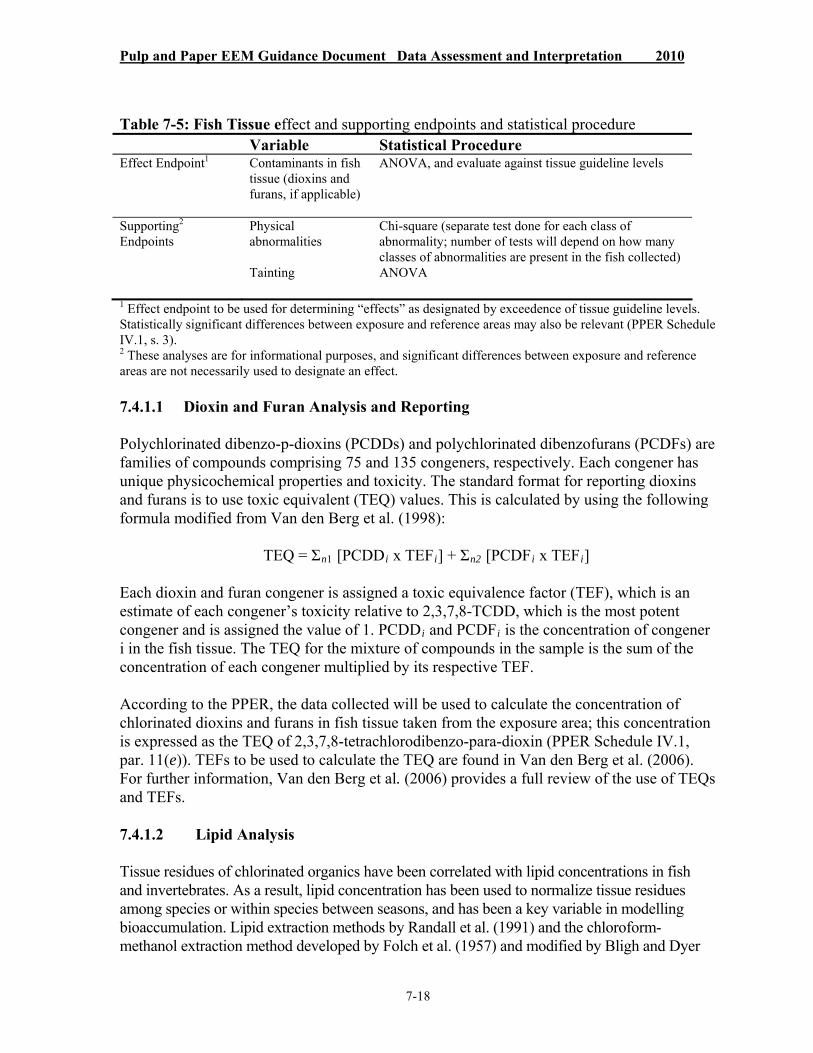
Pulp and Paper EEM Guidance Document Data Assessment and Interpretation 2010
7-18
Table 7-5: Fish Tissue effect and supporting endpoints and statistical procedure Variable Statistical Procedure
Effect Endpoint1 Contaminants in fish tissue (dioxins and furans, if applicable)
ANOVA, and evaluate against tissue guideline levels
Supporting2 Endpoints
Physical abnormalities
Chi-square (separate test done for each class of abnormality; number of tests will depend on how many classes of abnormalities are present in the fish collected)
Tainting ANOVA
1 Effect endpoint to be used for determining “effects” as designated by exceedence of tissue guideline levels. Statistically significant differences between exposure and reference areas may also be relevant (PPER Schedule IV.1, s. 3). 2 These analyses are for informational purposes, and significant differences between exposure and reference areas are not necessarily used to designate an effect.
7.4.1.1 Dioxin and Furan Analysis and Reporting
Polychlorinated dibenzo-p-dioxins (PCDDs) and polychlorinated dibenzofurans (PCDFs) are families of compounds comprising 75 and 135 congeners, respectively. Each congener has unique physicochemical properties and toxicity. The standard format for reporting dioxins and furans is to use toxic equivalent (TEQ) values. This is calculated by using the following formula modified from Van den Berg et al. (1998):
TEQ = Σn1 [PCDDi x TEFi] + Σn2 [PCDFi x TEFi]
Each dioxin and furan congener is assigned a toxic equivalence factor (TEF), which is an estimate of each congener’s toxicity relative to 2,3,7,8-TCDD, which is the most potent congener and is assigned the value of 1. PCDDi and PCDFi is the concentration of congener i in the fish tissue. The TEQ for the mixture of compounds in the sample is the sum of the concentration of each congener multiplied by its respective TEF.
According to the PPER, the data collected will be used to calculate the concentration of chlorinated dioxins and furans in fish tissue taken from the exposure area; this concentration is expressed as the TEQ of 2,3,7,8-tetrachlorodibenzo-para-dioxin (PPER Schedule IV.1, par. 11(e)). TEFs to be used to calculate the TEQ are found in Van den Berg et al. (2006). For further information, Van den Berg et al. (2006) provides a full review of the use of TEQs and TEFs.
7.4.1.2 Lipid Analysis
Tissue residues of chlorinated organics have been correlated with lipid concentrations in fish and invertebrates. As a result, lipid concentration has been used to normalize tissue residues among species or within species between seasons, and has been a key variable in modelling bioaccumulation. Lipid extraction methods by Randall et al. (1991) and the chloroform-methanol extraction method developed by Folch et al. (1957) and modified by Bligh and Dyer

Pulp and Paper EEM Guidance Document Data Assessment and Interpretation 2010
7-19
(1959) are recommended.
Percent lipid and percent moisture determinations should be provided for every sample submitted for chlorinated dioxins and furans analysis. Also, percent lipid values should be reported for the replicates analyzed in the same batch with the submitted sample. The percent lipid precision for the replicate samples should be ± 30% for tissues containing more than 2% lipid and ± 60% for tissues with less than 2% lipid. The method for the lipid determinations should be reported and the solvents used should be clearly specified.
7.4.2 Physical Abnormalities
Fish usability can be affected by altered appearance of fish. The data collected during the biological monitoring studies shall be used to identify the sex of the fish sampled and the presence of any lesions, tumours, parasites or other abnormalities (PPER Schedule IV.1, par. 11(b)). Obvious abnormalities may include:
tumours and/or lesions on the body surface (including the eyes, lips, snout, gills); spinal column malformations; eroded, frayed or hemorrhagic fins; other physical malformations; or obvious parasites.
For each class of abnormality that has been noted, a comparison between reference- and exposure-area fish should then be done using a chi-square goodness-of-fit test for relative frequencies. This information is used to help interpret effects, although, for EEM purposes, a significant difference does not necessarily signify an effect. The number of statistical tests that are necessary will depend on the number of classes of abnormalities that are noted in the collected fish. Sample size will have been determined by the number of fish collected for the fish survey. Cohen (1988) provides guidance on the power of a chi-square test that would result from that level of replication.

Pulp and Paper EEM Guidance Document Data Assessment and Interpretation 2010
7-20
7.5 Data Assessment and Interpretation for the Benthic Invertebrate Community Study
The data collected during the benthic invertebrate community survey shall be used to determine the following effect indicators (PPER Schedule IV.1, subpar. 11(a)(ii)):
1) total benthic invertebrate density; 2) the evenness index; 3) taxa richness; and 4) the similarity index (Bray-Curtis Index).
The above effect indicators are to be used for determining statistically significant differences between exposure and reference areas or along an exposure gradient. See Chapter 4 for additional information on these effect indicators. The mean, SD, SE, and minimum and maximum values are determined for each effect endpoint for the sampling areas. In addition, an analysis of the results shall be used to determine if there is a statistical difference between the sampling areas for each of the effect indicators (PPER Schedule IV.1, subpar. 11(a)(ii)).
7.5.1 Study Design and Statistical Procedures
Table 7-6 outlines the appropriate statistical procedures that are applicable for analysis for each of the recommended study designs. See Chapter 4 for additional information on these study designs. In contrast to the fish survey, the statistical procedure used to determine whether there has been an effect is dependent on which of the seven study designs is employed. For a given study, all four effect indicators are analyzed using the same study-design-determined statistical procedure. The one exception is the Reference Condition Approach, which uses a different set of statistical procedures that do not require inter-area comparisons of these four indicators, unless accompanied by ANOVAs; the procedures for this study design are outlined below and in Chapter 4.
Table 7-6: Statistical procedure used to determine an effect for each of the seven study designs Study Design Statistical Procedure
Control-Impact (C-I) ANOVA
Multiple Control-Impact (MC-I) ANOVA
Before/After Control-Impact (BACI) ANOVA
Simple Gradient (SG) Regression/ANOVA
Radial Gradient (RG) Regression/ANOVA
Multiple Gradient (MG) ANCOVA
Reference Condition Approach (RCA) Multivariate/ANOVA

Pulp and Paper EEM Guidance Document Data Assessment and Interpretation 2010
7-21
Note: Multivariate analyses can be performed on data collected using any of the designs in Table 7-6, to look for patterns that may be useful for highlighting potential areas of concern. Under certain circumstances, ANCOVAs may also be appropriate for any of these designs (e.g., to factor out the effect of a potentially confounding environmental variable).
Although it is possible to use ANOVA to analyze data collected under most of the study designs listed in Table 7-6, ANOVA is most applicable to the control-impact (C-I) and multiple control-impact (MC-I) designs. The simplest of these study designs is the C-I (or reference/exposure) design. In rivers, for example, this consists of one (usually upstream) reference area and one or more downstream exposure areas. Chapter 4 provides guidance on the different ways that C-I designs can be laid out. This type of study design employs ANOVA comparisons between reference and exposure areas, with a significant difference signifying an effect.
The MC-I design is similar to the C-I design, except that it employs additional reference areas that are located in adjacent watersheds or bays where the sampled habitat is comparable to that found within the exposure area. This type of design helps to reduce problems with confounding factors (e.g., when a single reference area differs from an exposure area with respect to several environmental variables in addition to the point-source effluent). Analogous to a C-I design, a significant difference between an exposure area and the mean of the reference areas, as determined by ANOVA, would represent an effect.
ANCOVA can also be used for both C-I and MC-I designs to factor out covariates that may create “noise” that makes it difficult to make simple ANOVA comparisons of reference to exposure areas. For example, without the use of ANCOVA, differences in depth among stations within the reference and exposure areas may mask effluent-related differences that may exist between those areas. This may occur when the benthic invertebrate indicators change along a continuum of increasing depth, and when it is not possible to take all samples at identical depths. In this example, ANCOVA can be used to factor out the effect of the depth covariate so as to focus on the effect of effluent exposure. The same approach can be used for other covariates that influence the benthic invertebrate indicators along a continuum.
An improvement to the above C-I and MC-I designs is possible when data can be collected both before and after initiation of effluent discharge into the receiving water area. This kind of monitoring design has been termed a before/after control-impact (BACI) design (Schmitt and Osenberg 1996). Use of a BACI design helps to distinguish effluent effects from natural differences between reference and exposure areas that may have existed before the initiation of effluent discharge.
In its simplest form, a BACI design entails collecting monitoring data at least once, both before and after initiation of effluent discharge in both a reference and exposure area, with the data analyzed using an area-by-time factorial ANOVA (Green 1979). In this situation, evidence for an effluent effect is inferred when the area-by-time interaction term in the ANOVA is significant. When the reference and exposure areas have been sampled repeatedly during both the before and after periods, it is possible to use a BACI paired series

Pulp and Paper EEM Guidance Document Data Assessment and Interpretation 2010
7-22
analysis, in which case the potential effects are investigated by testing for a change in delta (difference between reference and exposure) from the before to after period (Schmitt and Osenberg 1996). The design can be further improved by incorporating multiple reference areas (Schmitt and Osenberg 1996; Underwood 1997).
In contrast to the C-I and MC-I designs, the simple gradient (SG) and radial gradient (RG) designs are more amenable to regression analysis. The assumptions for regression analysis are applicable to the analysis of the benthic invertebrate community data, and have already been outlined in the section 7.3.3.2 discussion on ANCOVA (regression is one component of ANCOVA).
For additional information on study designs, refer to chapters 2 and 4.
7.5.2 Data Treatment
As for the fish survey, the data should be reported in both graphical and tabular format for each area (reference and exposure area(s)) being summarized. The reported data will include the descriptive statistics (mean, SD, SE, and minimum and maximum values) as well as the sample sizes. Gradient data should be presented graphically as scatter plots of variable vs. distance from the effluent outfall. For gradient designs with no discrete “areas,” tabular presentation prior to the main analysis would be applicable to station-by-station summary statistics, with the sampling unit being field sub-samples rather than stations. Station-by-station summary statistics are also applicable to C-I–type designs in cases where field sub-samples are not pooled prior to taxon enumeration, although the key summary statistics are those that are calculated for whole areas (to help with interpreting significant differences [“effects”] among areas).
The same three main analysis steps outlined in section 7.3.3 should be followed to determine whether statistically significant “effects” have occurred:
1) The data should be inspected to see whether they satisfy the assumptions of the statistical test or procedure being used (ANOVA, ANCOVA, regression or multivariate analyses).
2) The appropriate statistical procedure would be performed following data inspection and any necessary transformations (or non-parametric alternative).
3) The key results for the effect indicators should then be presented to clearly indicate whether there has been an effect, with details on the nature of the effect (including direction and magnitude). Again, an effect is declared if the p-value is less than the a priori value determined, as outlined in section 7.6.
The same considerations and constraints discussed in section 7.4.3 for conducting ANOVA and ANCOVA analyses apply to benthic invertebrate community analyses using those two statistical procedures. Thus, data inspection, analysis and interpretation when using ANOVA or ANCOVA for the benthic invertebrate community survey should follow the generic recommendations provided in section 7.3.3.
Pulp and Paper EEM Guidance Document Data Assessment and Interpretation 2010
7-23
Gradient designs are particularly useful for 1) situations where rapid effluent dilution precludes the selection of an exposure area that is comparatively homogeneous in terms of effluent concentration and 2) determining how far along an effluent path the effects are observed (i.e., determining the geographical extent of “effects”). The geographic extent of “effects” can be determined graphically by plotting the response variable(s) against distance from the effluent outfall, and inspecting the data for an inflection point where the response variable asymptotes to the reference condition. Data from sampling stations arrayed in this manner could also be used, together with measured physicochemical data, in a multivariate analysis (e.g., ordination or clustering) that is used to identify which more distant stations tend to group with reference stations and which tend to group with clearly affected stations.
Both of these approaches (graphical plotting and multivariate analysis) look for patterns in the data to qualitatively determine the approximate geographic extent of an effect. That is, they do not necessarily entail hypothesis testing, and therefore, in the context of the EEM program, are not used to designate an effect sufficient to warrant follow-up action, but rather are used for informational purposes.
Nevertheless, statistical tests are possible for some gradients. In the simplest case, an effect would be declared if the slope of the regression of the variable against distance from the effluent source is significantly different than zero, or if the correlation coefficient is statistically significant (data transformations may be necessary to satisfy assumptions of linearity). In this case, the effect is a relatively uniform gradient of variable values away from the point source, rather than an effect in a given discrete area.
An effect can also be signified by a significant exposure vs. reference ANOVA difference when comparing a group of stations along the gradient close to the mill to “reference” stations along the gradient far from the mill. This is analogous to the C-I approach, and assumes some degree of uniformity in exposure within the exposure group of stations and within the “reference” group of stations. Furthermore, the two groups of stations would need to be far enough apart to represent clear differences in exposure, and a sufficient number of stations would need to be available for each group to attain the desired level of power. Based on the power analysis discussion in the following section, an initial recommendation is to have at least five fairly uniform stations relatively close to the mill (near-field equivalent) and five fairly uniform stations far enough from the mill to approximate a “reference” area (i.e., minimally affected by the effluent). Providing intermediate stations would likely necessitate a total of at least 15 gradient stations overall.
Regardless of the method of analysis, overall statistical power is usually improved by emphasizing station replication on the 2 ends of the gradient. Again, emphasis should also be placed on extending the gradient sufficiently far from the mill (as much as is feasible) to allow sampling of stations that are as minimally affected as possible (and that serve as approximate “reference” stations).
Given sufficient sub-samples per station, it is also possible to use ANOVA to determine the presence or absence of an effect for a given station. This would entail using field

Pulp and Paper EEM Guidance Document Data Assessment and Interpretation 2010
7-24
sub-samples as replicates (treating stations as areas) and making station-by-station ANOVA comparisons of more near-field stations along the gradient to more distant reference stations. This method of analysis could be used to determine where along the gradient an effect disappears at the given level of significance. This latter approach may, however, require extensive sampling effort, depending upon the number of stations along the gradient and the required (by power analysis) number of field sub-samples per station.
In cases where these kinds of statistical tests are not adequate for a given gradient design, a redesign of the monitoring program will be necessary to enable an appropriate statistical test during the next monitoring study. The redesign may entail increased replication focused on the key exposure and reference areas (or stations) that are to be compared (e.g., increased replication in the near-field area of greatest effluent exposure and in the more far-field area that best represents reference conditions).
In some cases, it may be necessary to compare exposure vs. reference gradients. This would be the case when a co-occurring (non–mill-related) environmental gradient (i.e., covariate) confounds effluent effects in the exposure area. By using a multiple gradient (MG) design, it may be possible to make statistical comparisons of the exposure area gradient to a similar (non–mill-related) environmental gradient in an unexposed reference area. The reference gradient should be as similar as possible in depth and habitat to the exposure area gradient. Potential effluent “effects” would be tested for by using ANCOVA to compare reference to exposure area regression elevations (or adjusted means), while factoring out the influence of the co-occurring environmental covariate.
For example, if the gradient in effluent exposure away from the mill was confounded by a co-occurring increase in depth, an ANCOVA comparison might be made to a reference area where the depth gradient is the same. If the slopes for the reference and exposure area regressions against the covariate (X = depth) are approximately equal, a significant difference in adjusted means would indicate an effect of the effluent on the effect indicator Y (e.g., taxon richness). Again, section 7.3 provides further guidance for ANCOVA analyses and the different ways these analyses can be used to indicate an effect.
7.5.3 Reference Condition Approach
The reference condition approach (RCA) is a study design that combines inspection of multivariate patterns in the data with assessments of whether exposure stations fall outside a given ordination probability ellipse for reference stations. The fundamental concept of the RCA is to establish a database of stations that represent unimpaired conditions (reference stations) at which biological and environmental attributes are measured. This database is used to develop predictive models that match a set of environmental variables to biological conditions. These predictive models then allow a set of environmental measurements to be made at a new station and used in the model to predict the expected biological condition at the new station. An assessment of whether there has been an effect at the exposure station is enabled by a comparison of the actual biological condition at the new (exposure area) station with conditions at the reference stations to which the new station is predicted as belonging.

Pulp and Paper EEM Guidance Document Data Assessment and Interpretation 2010
7-25
The reference condition database is established by an initial standardized sampling program at a wide variety of spatial scales. The same benthic macroinvertebrate sampling protocol is used in as many ecoregions and stream orders or lakes as are available in a catchment. A number of environmental variables are measured in conjunction with invertebrate sampling. The data are then subjected to a 3-step multivariate analysis in which:
1) a number of invertebrate groups are formed based on similarity of community structure; 2) biological data are correlated with environmental attributes, and an optimal set of
environmental variables is identified that can be used to predict group membership; and 3) the biological condition of test (exposure) stations is assessed by using the optimal set of
environmental variables to predict group membership.
How the test station fits, relative to the group to which it is predicted to belong, establishes whether and to what degree the station is different from the reference group. A station or group of stations that fall outside the statistically determined ordination probability ellipse for the reference stations signifies the presence of an effect. The boundaries of the reference ellipse should be set a priori based on some of the considerations discussed in section 7.6. A more complete discussion of the assumptions, procedures and interpretation of the RCA is available in Reynoldson et al. (1995, 2000) and Bailey et al. (2003).
It should be further noted that, depending on the timing and locations of an RCA sampling program, it may also be possible to use the resulting database to make ANOVA comparisons between reference and exposure areas in order to determine whether there has been an effect. This latter kind of analysis would be analogous to an MC-I design.
To summarize, an overall procedure similar to that outlined in section 7.3 should also be followed (with appropriate modifications) for the benthic invertebrate community survey. However, the power analysis is not applicable to graphical approaches and the RCA. Consequently, RCA studies should be designed in a way that provides an accurate and precise determination of reference conditions so as to maximize the likelihood of detecting departures from reference conditions at exposure stations, when they exist. The following elements may be included as part of an RCA study:
1) Preparing the analyses: QA/QC (including checks for data entry errors), summary of confounding factors, description of the sampling design and taxonomic level used, clear identification of the sampling units used for statistical comparisons (e.g., stations rather than field sub-samples), ensuring equivalence of sampling substrata, and sampling techniques among different reference and exposure areas being compared
2) Summary statistics (graphical and tabular presentation of means, etc., as described above)
3) Statistical analyses (hypothesis testing) to determine “effects” (ANOVA, ANCOVA, regression)
4) Graphical approaches (e.g., inspection of the shape of regression lines, which is used for inspecting patterns in the data rather than determining “effects”)

Pulp and Paper EEM Guidance Document Data Assessment and Interpretation 2010
7-26
5) Multivariate statistical analyses used for determining a) patterns in the data and b) the position in multivariate space of exposure stations relative to reference ordination probability ellipses; only b) is used to determine “effects”
6) Power analyses (not applicable to graphical approaches and RCA)
7.5.4 Supporting Endpoints
The following benthic invertebrate community supporting endpoints should also be reported, including means, SDs, SEs, minimum and maximum values, and sample sizes:
Simpson’s diversity taxon (e.g., family) density taxon (e.g., family) proportion taxon (e.g., family) presence/absence
Unlike the effect endpoints (total benthic invertebrate density, the evenness index, taxa richness and the similarity index), the above-listed variables are included as supporting endpoints and are not statistically analyzed to determine “effects.” They may, however, be used to interpret effects at later stages (e.g., determining the magnitude and causes of “effects”). These should be reported in both graphical and tabular format for each area (reference and exposure area(s)) being summarized. It should be noted that there may be other descriptors that may also be useful for the interpretation of monitoring data, on a site-specific basis (see Resh et al. 1995 for a review).
7.6 The Role of Power Analysis, , and Critical Effect Size in Determining Effects
7.6.1 Setting and
In testing whether exposure areas differ significantly from reference areas, a low probability of a Type I error () is usually allowed so that a normal population or community will not be mistaken for an affected one. However, the monitoring program should also be designed to provide a reasonably high probability of statistically detecting a predetermined CES if it has occurred, i.e., the power of the test should be high. Power is 1-, where is the Type II error (see below).
Type I error is partially kept in check by setting a broad margin for variation around what is considered “healthy.” Sufficient sampling effort should also be expended to reduce Type II error, taking into account the low probability allowed for Type I error. Thus, to determine what sampling effort is required, the CES and the Type I and Type II error will all be taken into account and set a priori. That is, decisions should be made about the magnitude of Type I and Type II errors that are acceptable for determining power and thus the sampling effort required to detect the recommended CES.

Pulp and Paper EEM Guidance Document Data Assessment and Interpretation 2010
7-27
Type I error occurs (at probability ) if the null hypothesis that there is no effect is rejected when in fact it is true (e.g., an exposure area is declared as being different from reference when it is not).
Type II error occurs (at probability ) if the null hypothesis is accepted when it is false (e.g., the exposure area is declared as not being significantly different from reference when it is actually impaired). Therefore, is the risk to industry and is the risk to the environment.
The power of a statistical test is 1-, the probability associated with correctly rejecting the null hypothesis when it is false (e.g., the probability associated with correctly identifying an impaired area). In a well-designed, properly replicated monitoring program, the goal is to keep and low and power high.
As can be seen from the equation given later in this section, one way to increase power, given a fixed sampling effort (i.e., sample size), is to increase , i.e., there are trade-off decisions to be made when setting and . Traditionally, has been set at 0.05 for experimental studies where, in many cases, the cost of a Type II error is not particularly high. That is, an of 0.05 is typically used in situations where the primary concern is to have maximal confidence that a statistically significant effect is real. On the other hand, there is much less consensus and available literature on what is an appropriate level for . Some studies have suggested using a minimal power of 0.8 (i.e., = 0.2) (Alldredge 1987; Cohen 1988; Burd et al. 1990; Osenberg et al. 1994; Keough and Mapstone 1995).
In many cases, “this rule of thumb” can be traced back to Cohen’s seminal work on power analysis (see Cohen 1988), which is primarily geared toward applications in the behavioural sciences. For those types of applications, Cohen contended that Type I errors were likely to be more serious than Type II errors for cases where the biggest concern is to not propagate erroneous conclusions based on incorrect declarations of significant differences. Specifically, he suggested that, if Type I errors were to be considered four times more serious, it might be reasonable to set at the traditional (in terms of experimental studies) 0.05 and at 4 x 0.05 = 0.2. He cautioned, however, that this rule of thumb should be ignored for other types of studies where these assumptions are not applicable.
This latter caveat applies to environmental monitoring studies where, because of the potentially high cost (both ecological and monetary) of failing to detect negative impacts, many researchers in the field of biomonitoring argue that should be set at least to the same level as (e.g., Alldredge 1987; Underwood 1993; Mapstone 1995). That is, the argument has been widely made that, barring extenuating circumstances, the risk to the environment should not be set greater than that to industry. This suggests that the most reasonable starting point is to set = , and this position has been adopted by the EEM program. On a site-specific basis, it may sometimes be decided to 1) set > if it can be shown that the risk to the environment is of greater concern than the risk to industry, or to 2) set < if it can be shown that the risk to industry is of greater concern.
After deciding to set = , it is necessary to make a decision on an appropriate value for
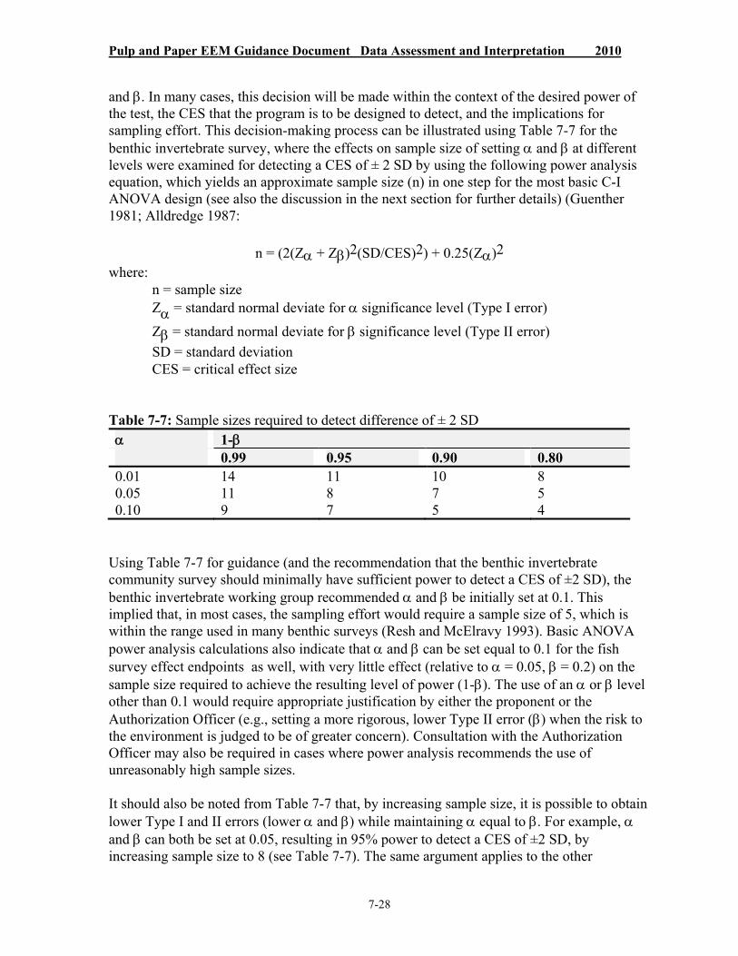
Pulp and Paper EEM Guidance Document Data Assessment and Interpretation 2010
7-28
and . In many cases, this decision will be made within the context of the desired power of the test, the CES that the program is to be designed to detect, and the implications for sampling effort. This decision-making process can be illustrated using Table 7-7 for the benthic invertebrate survey, where the effects on sample size of setting and at different levels were examined for detecting a CES of ± 2 SD by using the following power analysis equation, which yields an approximate sample size (n) in one step for the most basic C-I ANOVA design (see also the discussion in the next section for further details) (Guenther 1981; Alldredge 1987:
n = (2(Z + Z)2(SD/CES)2) + 0.25(Z)2
where: n = sample size Z = standard normal deviate for significance level (Type I error)
Z = standard normal deviate for significance level (Type II error)
SD = standard deviation CES = critical effect size
Table 7-7: Sample sizes required to detect difference of ± 2 SD 1-
0.99 0.95 0.90 0.80 0.01 14 11 10 80.05 11 8 7 50.10 9 7 5 4
Using Table 7-7 for guidance (and the recommendation that the benthic invertebrate community survey should minimally have sufficient power to detect a CES of ±2 SD), the benthic invertebrate working group recommended and be initially set at 0.1. This implied that, in most cases, the sampling effort would require a sample size of 5, which is within the range used in many benthic surveys (Resh and McElravy 1993). Basic ANOVA power analysis calculations also indicate that and can be set equal to 0.1 for the fish survey effect endpoints as well, with very little effect (relative to = 0.05, = 0.2) on the sample size required to achieve the resulting level of power (1-). The use of an or level other than 0.1 would require appropriate justification by either the proponent or the Authorization Officer (e.g., setting a more rigorous, lower Type II error () when the risk to the environment is judged to be of greater concern). Consultation with the Authorization Officer may also be required in cases where power analysis recommends the use of unreasonably high sample sizes.
It should also be noted from Table 7-7 that, by increasing sample size, it is possible to obtain lower Type I and II errors (lower and ) while maintaining equal to . For example, and can both be set at 0.05, resulting in 95% power to detect a CES of ±2 SD, by increasing sample size to 8 (see Table 7-7). The same argument applies to the other

Pulp and Paper EEM Guidance Document Data Assessment and Interpretation 2010
7-29
components of EEM (e.g., the fish survey and fish usability components) for different desired CESs, although the required sample sizes will be different. Thus, setting equal to provides an economic incentive to carrying out a well-designed, well-replicated monitoring program, because providing sufficient replication will help reduce the probability of Type I errors (i.e., is kept low), thereby reducing the probability of unnecessary follow-up studies. Furthermore, since is linked to , the power of the monitoring program to detect real effects will also be increased. This improvement in monitoring design helps to ensure a better understanding of what types of effects, if any, are occurring.
7.6.2 Power Analysis: Determination of Required Sample Size, Power and Appropriate Critical Effect Size
Power analysis is used for two major purposes during EEM:
1) at the beginning of a monitoring study (a priori), to calculate the sampling effort (sample size) that will be required to detect a given CES at a given level of power; and
2) following a recently completed monitoring study (post hoc), to determine the level of power that was actually achieved.
Both of these uses of power analysis are briefly reviewed here to help clarify the relationship between the two.
7.6.2.1 A Priori Power Calculations
During the initial design phase of an EEM study, power analysis can be used to determine the sample size required to achieve a test adequate to detect an effect equal to a predetermined CES prior to sampling. Using the CES, the probability of Type I error “,” the probability of type II error “,” an estimate of reference variability (e.g., SD for the reference area), and making some assumptions about the distribution of the data being evaluated, a scientifically defensible sampling strategy can be devised. The discussion below outlines the most basic (i.e., C-I ANOVA or ANCOVA) procedure for determining required sample size. Sample size refers to the number of fish for the fish survey and the number of stations for the benthic invertebrate community survey. In cases where the required sample size calculated for one effect endpoint (e.g., invertebrate density/condition) is greater than that calculated for another (e.g., invertebrate taxon richness / relative gonad weight), the greater sample size should be used (unless, as discussed above, consultation with the Authorization Officer confirms that this would result in excessively high sample sizes).
Once CES has been determined, the levels of and have been selected, and SD for the particular mill location in question has been estimated, they are entered into the power analysis equation to calculate the sample size required to detect an impact of magnitude CES between or among areas at a given power level. For the case where CES is set at ± 2SD, due to cancelling of terms the determination of SD is not required for the power analysis, and Table 7-7 above gives pre-calculated sample sizes for various values of and .

Pulp and Paper EEM Guidance Document Data Assessment and Interpretation 2010
7-30
It should be noted that determination of required sample size assumes that the variability among replicates for the exposure area is similar to that for the reference area. Although ANOVAs are fairly robust with respect to violation of normality assumptions, if the variance within an exposure area is much higher (or lower) than within the reference area, ANOVA comparisons may not be appropriate unless the variances can be made homogeneous by transformation. For the case where the exposure and reference variances remain significantly different following transformation, the power analysis outlined here may overestimate or underestimate the number of sampling stations required. Non-parametric tests may be used in this case; non-parametric power analyses would then be required to estimate required sampling effort (Thomas and Krebs 1997).
For a basic C-I ANOVA or ANCOVA design, the estimated sample size required to detect a given CES at a given power level can be calculated by arranging the standard power analysis equation as follows (Green 1989):
n = 2( t + t )2(SD/CES)2
where: n = sample size t = value of Student’s t statistic (two-tailed) with (n-1) degrees of freedom (df) at a
significance level of α t = value of Student’s t statistic (one-tailed) with (n-1) df at a significance level of β
SD = standard deviation CES = critical effect size, represented in the measurement units of the response variable
The equation is solved iteratively by choosing an approximate value of n (usually 20 for the fish survey) to look up t and t and then using the solution to find a more accurate n; the
procedure is repeated until arriving at a final estimate for n (see section A1-8 of Appendix 1). Alternatively, the equation given in section 7.6.1 can be used to approximately solve for n in one step. Pre-calculated tables of n (expanding upon Table 7-7) are available for a variety of values of , and CES (Alldredge 1987; Cohen 1988).
The reader is referred to the appropriate literature (e.g., Cohen 1988) for guidance on power analysis and tables for determining sample size for regression (simple gradient, radial gradient) and chi-square (analysis of physical abnormalities in fish) monitoring designs. A number of software programs are also available for conducting power analyses for a variety of statistical designs (Thomas and Krebs 1997). As for a basic C-I design, power analysis for these other designs will also require an a priori decision on an appropriate magnitude for CES. For regression analyses, Cohen (1988) gives a table for converting CESs from SD units to a correlation coefficient (r), and in some cases it may be acceptable to use this r to look up the approximate sample size required for a regression-type gradient design. For example, given certain assumptions, he shows that using a CES of 2 SD is equivalent to using r = 0.707 (or r2 = 0.5). Although the exact equivalency depends on the assumptions involved, it may be acceptable to use this conversion (possibly with a correction factor) to obtain an
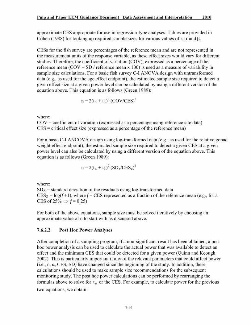
Pulp and Paper EEM Guidance Document Data Assessment and Interpretation 2010
7-31
approximate CES appropriate for use in regression-type analyses. Tables are provided in Cohen (1988) for looking up required sample sizes for various values of r, and .
CESs for the fish survey are percentages of the reference mean and are not represented in the measurement units of the response variable, as these effect sizes would vary for different studies. Therefore, the coefficient of variation (COV), expressed as a percentage of the reference mean (COV = SD / reference mean x 100) is used as a measure of variability in sample size calculations. For a basic fish survey C-I ANOVA design with untransformed data (e.g., as used for the age effect endpoint), the estimated sample size required to detect a given effect size at a given power level can be calculated by using a different version of the equation above. This equation is as follows (Green 1989):
n = 2(t + t)2 (COV/CES)2
where: COV = coefficient of variation (expressed as a percentage using reference site data) CES = critical effect size (expressed as a percentage of the reference mean)
For a basic C-I ANCOVA design using log-transformed data (e.g., as used for the relative gonad weight effect endpoint), the estimated sample size required to detect a given CES at a given power level can also be calculated by using a different version of the equation above. This equation is as follows (Green 1989):
n = 2(t + t)2 (SDz/CESz)2
where: SDZ = standard deviation of the residuals using log-transformed data CESZ = log(f +1), where f = CES represented as a fraction of the reference mean (e.g., for a CES of 25% f = 0.25)
For both of the above equations, sample size must be solved iteratively by choosing an approximate value of n to start with as discussed above.
7.6.2.2 Post Hoc Power Analyses
After completion of a sampling program, if a non-significant result has been obtained, a post hoc power analysis can be used to calculate the actual power that was available to detect an effect and the minimum CES that could be detected for a given power (Quinn and Keough 2002). This is particularly important if any of the relevant parameters that could affect power (i.e., n, α, CES, SD) have changed since the beginning of the study. In addition, these calculations should be used to make sample size recommendations for the subsequent monitoring study. The post hoc power calculations can be performed by rearranging the formulas above to solve for t or the CES. For example, to calculate power for the previous
two equations, we obtain:

Pulp and Paper EEM Guidance Document Data Assessment and Interpretation 2010
7-32
t =n
2(COV/CES)2 - t
and
t =n
2(SDz / CESz)2
- t
Power can then be obtained from the calculated value of t .
7.7 Critical Effect Sizes
To ensure that increased monitoring efforts are focused in the appropriate areas, Environment Canada has developed CESs for key fish and benthic invertebrate survey effect endpoints. See Chapter 1 for the table on CESs and for additional information.
7.8 Statistical Considerations for Mesocosm Studies
Some considerations would be unique to a mesocosm-type study. For example, control over experimental considerations would likely result in lower levels of variability within reference and exposure treatments, as compared with field data. This may make it possible to attain equivalent levels of statistical power using smaller sample sizes than used in the field. In the same vein, it may be possible to attain higher power levels or to detect smaller effect sizes while using the same sample sizes as used in the field. In fact, it may be desirable to have sufficient power to detect smaller effect sizes in mesocosm studies than in field surveys, due to the shorter exposure times typical of mesocosm studies. That is (using hypothetical numbers), a 10% effluent-induced change over a 30-day exposure period in a mesocosm study may be equivalent to a 25% change over a much longer lifetime exposure in the field.
In addition, due to the possibility of caging artifacts, it may be necessary to switch from using individual fish as the sampling unit for replication (as in the field) to using individual experimental enclosures (mesocosms) as sampling units. Using two mesocosm units (one for reference and one for exposure) with 20 fish each may not be valid, because it may not be possible to separate effluent effects from the effects due to subtle differences in the experimental enclosures. This is an example of the potential for confounding effects due to pseudo-replication (Hurlbert 1984).
In comparison to the fish survey, it may be even more straightforward to substitute mesocosm studies for benthic invertebrate community field monitoring, at least in terms of statistical design and analysis. As for the fish survey, the same steps outlined for data preparation, presentation and analysis would apply. Furthermore, due to comparatively fast turnaround times for changes in invertebrate community structure within mesocosms, it may

Pulp and Paper EEM Guidance Document Data Assessment and Interpretation 2010
7-33
be possible to use the same effect endpoints as used in the invertebrate field survey (section 7.5). The most likely study design would be analogous to the C-I design (Table 7-6), with ANOVA comparisons being made between replicated reference and exposure mesocosms. The sampling units would be the individual mesocosms (equivalent to “stations” in the field survey). As for fish mesocosms, control over variability under experimental conditions may make it possible to attain greater statistical power or to detect smaller effect sizes (in terms of percentage change) using the same sample sizes as typically used in the field. This increase in precision is one of the most frequently cited advantages of using mesocosms in place of field sampling, and is weighed against the disadvantage of a potential decrease in accuracy due to using a (hopefully realistic) simulation of actual field conditions.
Chapter 8 provides more extensive discussion on data assessment and interpretation for alternative methods.

Pulp and Paper EEM Guidance Document Data Assessment and Interpretation 2010
7-34
7.9 References
Alldredge JR. 1987. Sample size for monitoring of toxic chemical sites. Environ Monit Assess 9:143-154.
Bailey RC, Norris RH, Reynoldson TB. 2003. Bioassessment of freshwater ecosystems: using the reference condition approach. Boston (MA): Kluwer Academic Publishers.
Barrett TJ, Tingley MA, Munkittrick KR, Lowell RB. 2010. Dealing with heterogeneous regression slopes in analysis of covariance: new methodology applied to environmental effects monitoring fish survey data. Environ Monit Assess 166(1-4):279-291.
Bartlett JR, Randerson PF, Williams R, Ellis DM. 1984. The use of analysis of covariance in the back-calculation of growth in fish. J Fish Biol 24:201-213.
Bligh EG, Dyer W. 1959. A rapid method of total lipid extraction and purification. Can J Biochem Physiol 37:911–917.
Bolger T, Connolly PL. 1989. The selection of suitable indices for the measurement and analysis of fish condition. J Fish Biol 34: 171-182.
Burd BJ, Nemec A, Brinkhurst RO. 1990. The development and application of analytical methods in benthic marine infaunal studies. Adv Mar Biol 26:169-247.
Cohen J. 1988. Statistical power analysis for the behavioral sciences. 2nd ed. Hillsdale (NJ): Lawrence Erlbaum Associates.
Cook RD. 1977. Detection of influential observation in linear regression. Technometrics 19:15-18.
Cook RD. 1979. Influential observations in linear regression. J Amer Stat Assoc 74:169-174.
Day RW, Quinn GP. 1989. Comparisons of treatments after an analysis of variance in ecology. Ecol Monogr 59:433–463.
Draper NR, Smith H. 1981. Applied regression analysis. 2nd ed. New York (NY): John Wiley & Sons, Inc.
Environment Canada. 1997. Fish survey expert working group report. EEM/1997/6. Ottawa (ON): Environment Canada.
Folch J, Lees M, Sloane Stanley GH. 1957. A simple method for the isolation and purification of total lipides from animal tissues. J Biol Chem 226:497-509.
Fox J. 1997. Applied regression analysis, linear model, and related models. Thousand Oaks (CA): Sage Publications Inc.

Pulp and Paper EEM Guidance Document Data Assessment and Interpretation 2010
7-35
Gibbons DW, Reid JB, Chapman RA. 1993. The New Atlas of Breeding Birds in Britain and Ireland: 1988–1991. London (UK): Poyser.
Gray MA, Curry AR, Munkittrick KR. 2002. Non-lethal sampling methods for assessing environmental impacts using a small-bodied sentinel fish species. Water Qual Res J Can 37:195-211.
Green RH. 1979. Sampling design and statistical methods for environmental biologists. New York (NY): Wiley-Interscience.
Green RH. 1989. Power analysis and practical strategies for environmental monitoring. Environ Res 50:195-205.
Grubbs F. 1969. Procedures for detecting outlying observations in samples. Technometrics 11:1-21.
Guenther WC. 1981. Sample size formulas for normal theory T tests. Am Stat 35:243-244.
Hamilton BL. 1977. An empirical investigation of the effects of heterogeneous regression slopes in analysis of covariance. Educ Psychol Meas 37:701-712.
Hubert JJ. 1980. Bioassay. Dubuque (IA): Kendall/Hunt Publishing.
Huitema BE. 1980. The analysis of covariance and alternatives. New York (NY): John Wiley & Sons, Inc.
Hurlbert SH. 1984. Pseudoreplication and the design of ecological field experiments. Ecol Monogr 54:187-211.
Iman, R.L., Conover, W.J. 1982. A distribution-free approach to inducing rank
correlation among input variables. Commun. Statist.-Simula. Computa. 11, 311-334.
Jackson DA, Harvey HH, Somers KM. 1990. Ratios in aquatic sciences: statistical shortcomings with mean depth and the morphoedaphic index. Can J Fish Aquat Sci 47:1788-1795.
Keough MJ, Mapstone BD. 1995. Protocols for designing marine ecological monitoring associated with BEK mills. )Technical Report Series 11). National Pulp Mills Research Program. Canberra (AU): Commonwealth Scientific and Industrial Research Organisation.
Lowell RB, Kilgour BW. 2008. Interpreting effluent effects on fish when the magnitude of effect changes with size or age of fish. dans K.A. Kidd, R. Allen Jarvis, K. Haya, K. Doe et L.E. Burridge (éd.), Compes rendus du 34ième atelier annuel sur la toxicité aquatique: du 30 septembre au 3 octobre 2007, Halifax, Nouvelle-Écosse.Can Tech Rep Fish Aquat Sci 2793:82-83.
Mapstone BD. 1995. Scalable decision rules for environmental impact studies: effect size, Type I and Type II errors. Ecol Appl 5:401-410.

Pulp and Paper EEM Guidance Document Data Assessment and Interpretation 2010
7-36
Miller RG. 1986. Beyond ANOVA: Basics of applied statistics. New York (NY): John Wiley & Sons, Inc.
Osenberg CW, Schmitt RJ, Holbrook SJ, Abu-Saba KE, Flegal AR. 1994. Detection of environmental impacts: natural variability, effect size and power analysis. Ecol Appl 4:16-20.
Paine RT, Tegner MJ, Johnson EA. 1998. Compounded perturbations yield ecological surprises. Ecosystems 1:535–545.
Peters RH. 1983. The ecological implication of body size. New York (NY): Cambridge University Press. 329 pp.
Quade D. 1967. Rank analysis of covariance. J Amer Stat Assoc 62:1187-1200.
Quinn GP, Keough MJ. 2002. Experimental design and data analysis for biologists. Cambridge (UK): Cambridge University Press.
Randall R, Lee II H, Ozretich R, Lake J, Pruell J. 1991. Evaluation of selected lipid methods for normalizing pollutant bioaccumulation. Environ Toxicol Chem 10:1431-1436.
Resh VH, McElravy EP. 1993. Contemporary quantitative approaches to biomonitoring using benthic macroinvertebrates. In: Rosenberg DM, Resh VH, editors. Freshwater biomonitoring and benthic macroinvertebrates. New York (NY): Chapman and Hall. p. 159-194.
Resh VH, Norris RH, Barbour MT. 1995. Design and implementation of rapid assessment approaches for water resource monitoring using benthic macroinvertebrates. Austral J Ecol 20:108-121.
Reynoldson TB, Bailey RC, Day KE, Norris RH. 1995. Biological guidelines for freshwater sediment based on benthic assessment of sediment (the BEAST) using a multivariate approach for predicting biological state. Austral J Ecol 20:198-219.
Reynoldson TB, Day KE, Pascoe T. 2000. The development of the BEAST: a predictive approach for assessing sediment quality in the North American Great Lakes. In: Wright JF, Sutcliffe DW, Furse MT, editors. Assessing the biological quality of fresh waters: RIVPACS and other techniques. Ambleside (UK): Freshwater Biological Association. p. 165-180.
Ricker WE. 1975. Computation and interpretation of biological statistics of fish populations. Bull Fish Res Board Can (23)2:519–529.
Schmitt RJ, Osenberg CW. 1996. Detecting ecological impacts: concepts and applications in coastal marine habitats. San Diego (CA): Academic Press. 401p.
Shirley EAC. 1981. A distribution-free method for analysis of covariance based on ranked data. Appl Stat 30:158-162.

Pulp and Paper EEM Guidance Document Data Assessment and Interpretation 2010
7-37
Sokal RR, Rohlf FJ. 1995. Biometry. 3rd ed. New York (NY): W.H. Freeman.
Thomas L, Krebs CJ. 1997. A review of statistical power analysis software. Bull Ecol Soc Am 78:126-139.
Trippel EA, Harvey HH. 1991. Comparison of methods used to estimate age and length of fishes at sexual maturity using populations of white sucker (Catostomus commersoni). Can J Fish Aquat Sci 48:1446-1495.
Underwood AJ. 1993. The mechanics of spatially replicated sampling programmes to detect environmental impacts in a variable world. Austral J Ecol 18:99-116.
Underwood AJ. 1997. Experiments in ecology: their logical design and interpretation using analysis of variance. Cambridge (UK): Cambridge University Press. 504 pp.
Van den Berg M, Birnbaum L, Bosveld AT, Brunstrom B, Cook P, Feeley M, Giesy JP, Hanberg A, Hasegawa R, Kennedy SW et al. 1998. Toxic equivalency factors (TEFs) for PCBs, PCDDs, PCDFs for humans and wildlife. Environ Health Perspect 106:775-792.
Van den Berg M, Birnbaum L, Denison M, De Vito M, Farland W, Feeley M, Fiedler H, Hakansson H, Hanberg A, Haws L et al. 2006. The 2005 World Health Organization re-evaluation of human and mammalian toxic equivalency factors for dioxins and dioxin-like compounds. Toxicol Sci 93:223-241.

Pulp and Paper EEM Guidance Document Data Assessment and Interpretation 2010
7-38
Appendix 1 Step-by-Step Guidance through Statistical Procedures
The following provides statistical background and step-by-step guidance through the statistical procedures required for the environmental effects monitoring (EEM) fish survey. This background material and the step-by-step procedures are meant as general guidance, and can be adapted to the particular statistical software package procedures that are being used. Examples are taken from different data sets from previous cycles to illustrate concepts where possible.
Analysis of covariance (ANCOVA) can be performed as multiple linear regression with indicator variables to represent sites. In an analysis with a reference (ref.) and an exposure (exp.) site, data can be fit to the regression model
y 0 1 x x1 2 2 3( )x1 x2 (1)
where y is the response, x1 is the covariate, x2 is an indicator variable for treatment (e.g.,
0 for reference and 1 for exposure), and x1 2 x is a covariate by treatment interaction term
which is equal to the product of the covariate and the indicator variable for each observation. This model fits the data to two regression lines with distinct intercepts and slopes, namely y 0 1 x1 for the reference site and y 0 2 1 3 x1 for the
exposure site. A test for parallel regression slopes is equivalent to testing the significance of the coefficient of the x1 x2 interaction term (i.e., a test of whether of3 = 0). If this
coefficient is not significant (at the α = 0.05 level of significance), the data can be described by two parallel lines with distinct intercepts. This model is
y 0 1 x1 2x2 . (2)
The test for differences in the response between treatments can proceed with (2). This test is equivalent to testing whether the two regression lines have equal intercepts (i.e., a test of whether2 = 0). If there is no significant difference in response between
treatments, the data can be represented by a single regression line without the2 term.
Thus, analyzing data using ANCOVA is equivalent to fitting the data to (1) to assess parallel slopes, and testing for differences among sites is equivalent to testing the significance of the2 in (2). Comparisons to critical effect sizes are made by comparing
the percentage difference in adjusted means (mean response adjusted to factor out differences in the covariate values) to predetermined critical effect sizes. This percentage difference can be easily calculated from (2). The coefficient2 in (2) is the vertical
distance between the two regression lines (i.e., the difference in intercepts) and can be converted into a percentage difference in the responses variable as

% difference = 102 1 100% (3)
when the response variable is log-transformed. The adjusted means can be calculated by evaluating (2) using the grand mean of the covariate (average covariate value over all sites) for x1 and using the appropriate indicator value for x2 to obtain each adjusted
mean if desired.
A1.1 Identifying Immature Fish
Calculate gonadosomatic index (GSI) = gonad weight / body weight x 100. Immature fish can typically be identified as those with GSI < 1%.
Plot gonad weight vs. body weight. Immature fish can usually be quickly identified.
Figure A1-1 illustrates a data set with several immature fish. A line representing GSI = 1% is added to help identify immature fish.
Scatterplot of Gonad Weight vs Body Weight
Figure A1-1: A plot of gonad weight vs. body weight for female Catostomus macrocheilus. Line represents GSI = 1%
Some fish species do not spawn every year. Some fish will not invest energy into reproduction every year. These species can be easily identified from plots of gonad weight vs. body weight where the data form two different groups corresponding to the spawning fish and non spawning fish. When a line of GSI = 1% is added to the plot, the spawning and non-spawning fish can be easily distinguished. See Figure A1-2.
Pulp and Paper EEM Guidance Document Data Assessment and Interpretation 2010
120010008006004002000
60
50
40
30
20
10
0
Body Weight
Gona
d W
eigh
t
ExpRef
Site
GSI = 1%
7-39

Pulp and Paper EEM Guidance Document Data Assessment and Interpretation 2010
Scatterplot of Gonad Weight vs Body Weight
Figure A1-2: A plot of gonad weight vs. body weight for female Lota lota. Line represents GSI = 1%
A1.2 Summary Statistics
Separate data by species, sex and site (e.g., reference or exposure). Plot each data set using a box plot and examine for obvious data entry errors or
any unusual observations.
Box plots for the length variable for female Catostomus commersoni are shown in Figure A1-3. The box plot in A reveals an unusually long fish at the exposure site. A review of field notes and comments in the spreadsheet indicate that this fish was exceptionally longer than all other fish. This observation lies considerably far outside the range of values for “Length” and may be considered an outlier.
800700600500400300
90
80
70
60
50
40
30
20
10
0
Body Weight
Gona
d W
eigh
t
ExpRef
Site
GSI = 1%
7-40
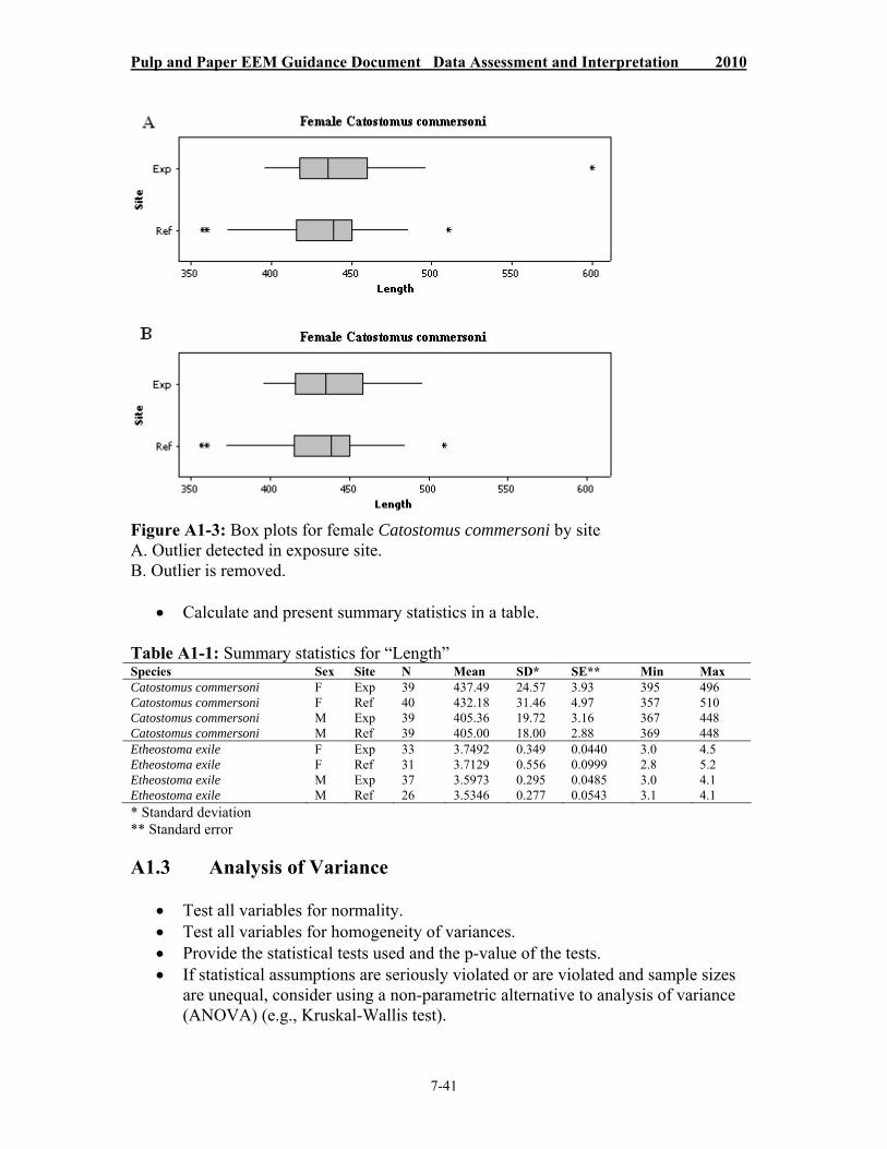
Pulp and Paper EEM Guidance Document Data Assessment and Interpretation 2010
7-41
Figure A1-3: Box plots for female Catostomus commersoni by site A. Outlier detected in exposure site. B. Outlier is removed.
Calculate and present summary statistics in a table.
Table A1-1: Summary statistics for “Length” Species Sex Site N Mean SD* SE** Min MaxCatostomus commersoni F Exp 39 437.49 24.57 3.93 395 496 Catostomus commersoni F Ref 40 432.18 31.46 4.97 357 510 Catostomus commersoni M Exp 39 405.36 19.72 3.16 367 448 Catostomus commersoni M Ref 39 405.00 18.00 2.88 369 448 Etheostoma exile F Exp 33 3.7492 0.349 0.0440 3.0 4.5 Etheostoma exile F Ref 31 3.7129 0.556 0.0999 2.8 5.2 Etheostoma exile M Exp 37 3.5973 0.295 0.0485 3.0 4.1 Etheostoma exile M Ref 26 3.5346 0.277 0.0543 3.1 4.1 * Standard deviation ** Standard error
A1.3 Analysis of Variance
Test all variables for normality. Test all variables for homogeneity of variances. Provide the statistical tests used and the p-value of the tests. If statistical assumptions are seriously violated or are violated and sample sizes
are unequal, consider using a non-parametric alternative to analysis of variance (ANOVA) (e.g., Kruskal-Wallis test).
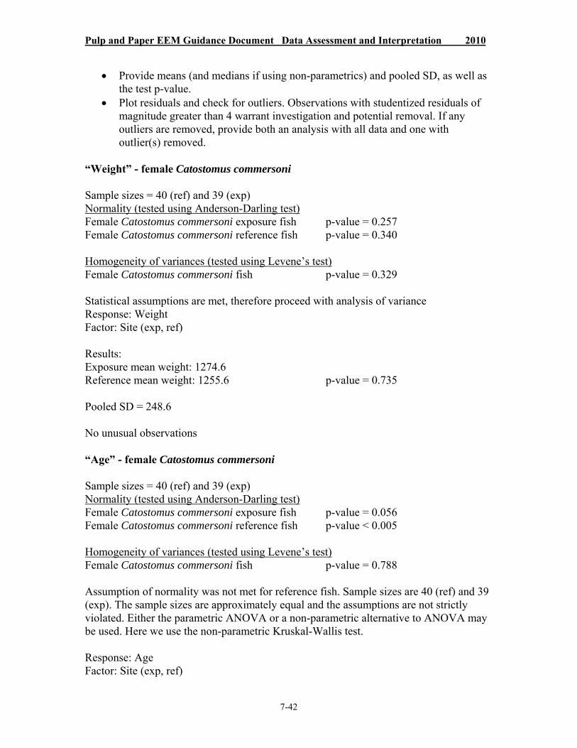
Pulp and Paper EEM Guidance Document Data Assessment and Interpretation 2010
7-42
Provide means (and medians if using non-parametrics) and pooled SD, as well as the test p-value.
Plot residuals and check for outliers. Observations with studentized residuals of magnitude greater than 4 warrant investigation and potential removal. If any outliers are removed, provide both an analysis with all data and one with outlier(s) removed.
“Weight” - female Catostomus commersoni
Sample sizes = 40 (ref) and 39 (exp) Normality (tested using Anderson-Darling test) Female Catostomus commersoni exposure fish p-value = 0.257 Female Catostomus commersoni reference fish p-value = 0.340
Homogeneity of variances (tested using Levene’s test) Female Catostomus commersoni fish p-value = 0.329
Statistical assumptions are met, therefore proceed with analysis of variance Response: Weight Factor: Site (exp, ref)
Results: Exposure mean weight: 1274.6 Reference mean weight: 1255.6 p-value = 0.735
Pooled SD = 248.6
No unusual observations
“Age” - female Catostomus commersoni
Sample sizes = 40 (ref) and 39 (exp) Normality (tested using Anderson-Darling test) Female Catostomus commersoni exposure fish p-value = 0.056 Female Catostomus commersoni reference fish p-value < 0.005
Homogeneity of variances (tested using Levene’s test) Female Catostomus commersoni fish p-value = 0.788
Assumption of normality was not met for reference fish. Sample sizes are 40 (ref) and 39 (exp). The sample sizes are approximately equal and the assumptions are not strictly violated. Either the parametric ANOVA or a non-parametric alternative to ANOVA may be used. Here we use the non-parametric Kruskal-Wallis test.
Response: Age Factor: Site (exp, ref)

Pulp and Paper EEM Guidance Document Data Assessment and Interpretation 2010
Studentized Residuals Versus Order(response is Length)
Results: Exposure median age: 10 Reference median age: 8 p-value = 0.001
“Length” - female Catostomus commersoni
Residual plot – studentized residuals vs. order (order data are entered in spreadsheet) Outliers are typically regarded as observations with magnitude > 4 and can be easily identified in this plot.
Figure A1-4: A plot of studentized residual vs. observation order (in spreadsheet) for the ANOVA on length for female Catostomus commersoni
A1.4 Analysis of Covariance (ANCOVA)
Plot the response variable vs. covariate for all sites. Inspect plot for a linear trend and appropriate overlap of covariate values. Inspect plot for outliers—calculate studentized residuals from ANCOVA model. Consider removing outliers with magnitude > 4 (studentized residual). Test residuals for normality (each regression line). Test residuals for homogeneity of variances (among regression lines). Test homogeneity of regression slopes—fit data to regression model with
interaction term and test significance of interaction term. Provide coefficient of determination “R2” for the regression model.
Test for differences in the response—fit data to regression model without interaction term and test significant of the site (treatment) term. Provide
80757065605550454035302520151051
5
4
3
2
1
0
-1
-2
-3
-4
-5
Observation Order
Stud
enti
zed
Res
idua
l
7-43
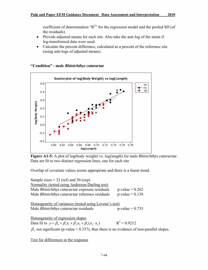
coefficient of determination “R2” for the regression model and the pooled SD (of the residuals).
Provide adjusted means for each site. Also take the anti-log of the mean if log-transformed data were used.
Calculate the percent difference, calculated as a percent of the reference site (using anti-logs of adjusted means).
“Condition” - male Rhinichthys cataractae
Scatterplot of log(Body Weight) vs log(Length)
Figure A1-5: A plot of log(body weight) vs. log(length) for male Rhinichthys cataractae. Data are fit to two distinct regression lines, one for each site
Overlap of covariate values seems appropriate and there is a linear trend.
Sample sizes = 32 (ref) and 30 (exp) Normality (tested using Anderson-Darling test) Male Rhinichthys cataractae exposure residuals p-value = 0.262 Male Rhinichthys cataractae reference residuals p-value = 0.138
Homogeneity of variances (tested using Levene’s test) Male Rhinichthys cataractae residuals p-value = 0.733
Homogeneity of regression slopes Data fit to y 0 1 x x1 2 2 3(x1 x2 ) R2 = 0.9212
3 not significant (p-value = 0.337), thus there is no evidence of non-parallel slopes.
Test for differences in the response
Pulp and Paper EEM Guidance Document Data Assessment and Interpretation 2010
7-44
0.780.760.740.720.700.680.660.640.620.60
0.5
0.4
0.3
0.2
0.1
0.0
-0.1
-0.2
log(Length)
log(
Body
Wei
ght)
ExpRef
Site

Data fit to y 0 1 x1 2x2 R2 = 0.9199
2 is significant (p-value = 0.0001), thus there is a significant difference in weight
between sites.
Adjusted mean for reference weight: 1.3113 g Adjusted mean for exposure weight: 1.4496 g (Means are anti-logged to obtain original units when log-transformed—the anti-log of x is 10x if the transformation was log base 10.)
Pooled SD = 0.0420164
Percent difference = 10.54% (calculated as percent of reference using adjusted means)
A1.5 Non-parallel Slopes in Analysis of Covariance
Method 1
“Relative gonad weight” – male Catostomus commersoni
Scatterplot of log(Gonad Weight) vs log(Body Weight)
Figure A1-6: A plot of log(gonad weight) vs. log(body weight) for male Catostomus commersoni. Data are fit to two distinct regression lines, one for each site
Overlap of covariate values seems appropriate and there is a linear trend. One observation warrants investigation in the exposure group.
A plot of the studentized residuals does not reveal any observations with extremely large magnitudes. See Figure A1-7.
Pulp and Paper EEM Guidance Document Data Assessment and Interpretation 2010
3.33.23.13.02.92.82.72.6
2.1
2.0
1.9
1.8
1.7
1.6
1.5
1.4
log(Body Weight)
log(
Gona
d W
eigh
t)
ExpRef
Site
7-45

Studentized Residuals vs log(Body Weight)
Figure A1-7: A plot of studentized residual vs. log(body weight) for male Catostomus commersoni data fit to the interaction model y 0 1 x x1 2 2 3( )x1 x2
Sample sizes = 29 (ref) and 25 (exp) Normality (tested using Anderson-Darling test) Male Catostomus commersoni exposure residuals p-value = 0.543 Male Catostomus commersoni reference residuals p-value = 0.176
Homogeneity of variances (tested using Levene’s test) Male Catostomus commersoni residuals p-value = 0.882
Homogeneity of regression slopes Data fit to y 0 1 x x1 2 2 3( )x1 x2 R2 = 0.7710
3 significant (p-value = 0.014), thus there is evidence of non-parallel slopes.
Assess influence by plotting Cook’s distance vs. the covariate.
Pulp and Paper EEM Guidance Document Data Assessment and Interpretation 2010
3.33.23.13.02.92.82.72.6
3
2
1
0
-1
-2
-3
log(Body Weight)
Stud
enti
zed
Res
idua
lExpRef
Site
7-46

Scatterplot of Cook's Distance vs log(Body Weight)
Figure A1-8: A plot of Cook’s distance vs. log(body weight) for male Catostomus commersoni data fit to the interaction model y 0 1 x x1 2 2 3( )x1 x2
One observation in the exposure group has a large Cook’s distance. Remove and test assumptions again.
Sample sizes = 29 (ref) and 24 (exp) Normality (tested using Anderson-Darling test) Male Catostomus commersoni exposure residuals p-value = 0.408 Male Catostomus commersoni reference residuals p-value = 0.176
Homogeneity of variances (tested using Levene’s test) Male Catostomus commersoni residuals p-value = 0.852
Homogeneity of regression slopes Data fit to y 0 1 x x1 2 2 3( )x1 x2 R2 = 0.7841
3 not significant (p-value = 0.205), thus there is no evidence of non-parallel slopes.
Continue with procedure.
Method 2
“Condition” - male Catostomus catostomus
Pulp and Paper EEM Guidance Document Data Assessment and Interpretation 2010
3.33.23.13.02.92.82.72.6
0.9
0.8
0.7
0.6
0.5
0.4
0.3
0.2
0.1
0.0
log(Body Weight)
Cook
's D
ista
nce
ExpRef
Site
7-47

Scatterplot of log(Body Weight) vs log(Length)
Figure A1-9: A plot of log(body weight) vs. log(length) for male Catostomus catostomus. Data are fit to two distinct regression lines, one for each site
Homogeneity of regression slopes Data fit to y 0 1 x x1 2 2 3(x1 x2 ) R2 = 0.8530
3 significant (p-value = 0.036), thus there is evidence of non-parallel slopes, but R2 >
0.8, thus fit parallel model and compare coefficients of determination.
Data fit to y 0 1 x x1 2 2 R2 = 0.8450
R2 for parallel model is also > 0.8 and is less than 0.02 (i.e. 2 percentage points) less than R2 for interaction model. Thus use parallel model to describe data and continue with analysis.
Pulp and Paper EEM Guidance Document Data Assessment and Interpretation 2010
1.3251.3001.2751.2501.2251.2001.1751.150
2.0
1.9
1.8
1.7
1.6
1.5
log(Length)
log(
Body
Wei
ght)
ExpRef
Site
7-48
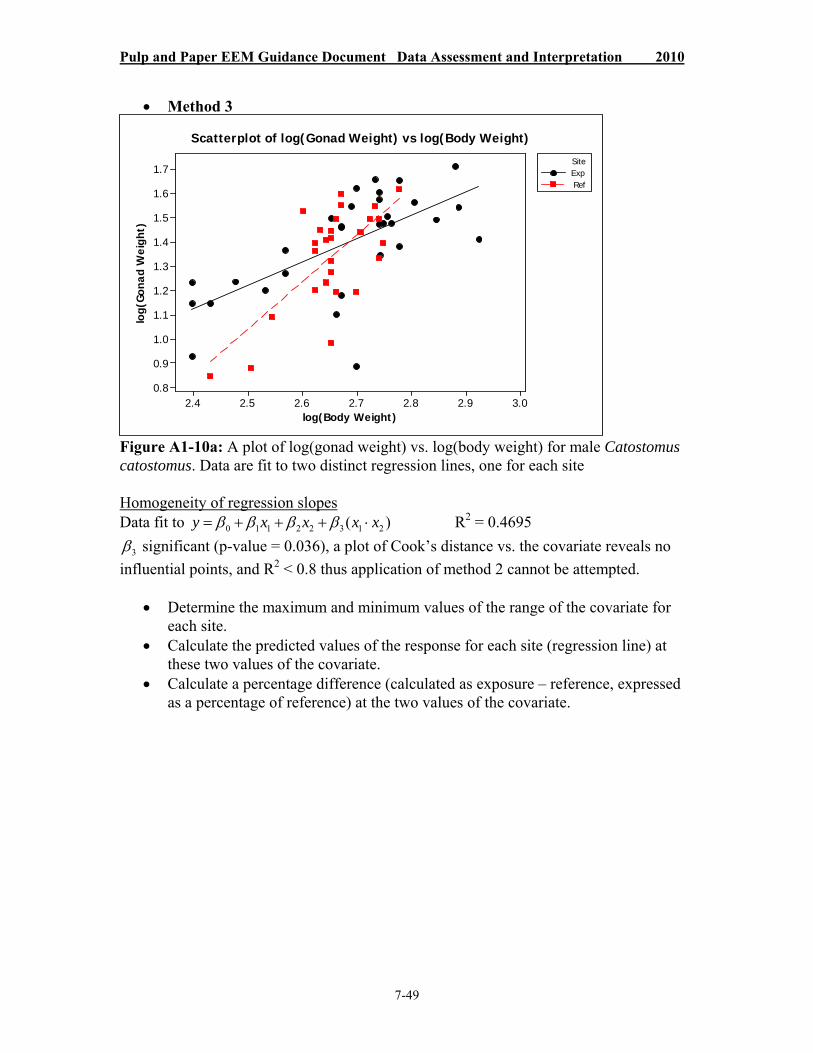
Method 3
Scatterplot of log(Gonad Weight) vs log(Body Weight)
Figure A1-10a: A plot of log(gonad weight) vs. log(body weight) for male Catostomus catostomus. Data are fit to two distinct regression lines, one for each site
Homogeneity of regression slopes Data fit to y 0 1 x x1 2 2 3( )x1 x2 R2 = 0.4695
3 significant (p-value = 0.036), a plot of Cook’s distance vs. the covariate reveals no
influential points, and R2 < 0.8 thus application of method 2 cannot be attempted.
Determine the maximum and minimum values of the range of the covariate for each site.
Calculate the predicted values of the response for each site (regression line) at these two values of the covariate.
Calculate a percentage difference (calculated as exposure – reference, expressed as a percentage of reference) at the two values of the covariate.
Pulp and Paper EEM Guidance Document Data Assessment and Interpretation 2010
3.02.92.82.72.62.52.4
1.7
1.6
1.5
1.4
1.3
1.2
1.1
1.0
0.9
0.8
log(Body Weight)
log(
Gona
d W
eigh
t)
ExpRef
Site
7-49

Scatterplot of log(Gonad Weight) vs log(Body Weight)
Figure A1-10b: The data from Figure 10a but with the minimum and maximum values of the range of overlap of the covariate between sites identified
Covariate values 2.4314 and 2.7782 For 2.4314: predicted values for the response are 1.0949 (ref) and 1.1544 (exp). For 2.7782: predicted values for the response are 1.4963 (ref) and 1.4883 (exp).
Thus percent differences are calculated to be (after taking the anti-log of the predicted response values) 14.69% and -1.84% for the covariate values of 2.4314 and 2.7782, respectively. These will be the estimates of the effects for smaller and larger fish, respectively, and can be compared to a critical effect size.
A1.6 Non-parametric ANCOVA
“Relative gonad weight” – female Catostomus commersoni
Pulp and Paper EEM Guidance Document Data Assessment and Interpretation 2010
3.02.92.82.72.62.52.4
1.7
1.6
1.5
1.4
1.3
1.2
1.1
1.0
0.9
0.8
log(Body Weight)
log(
Gona
d W
eigh
t)2.4314 2.7782
ExpRef
Site
7-50

Scatterplot of log(Gonad Weight) vs log(Body Weight)
Figure A1-11: A plot of log(gonad weight) vs. log(body weight) for female Catostomus commersoni. Data are fit to two distinct regression lines, one for each site
Distribution of covariate values for two sites are not very similar.
Sample sizes = 26 (ref) and 25 (exp) Normality (tested using Anderson-Darling test) Female Catostomus commersoni exposure residuals p-value = 0.476 Female Catostomus commersoni reference residuals p-value = 0.596
Homogeneity of variances (tested using Levene’s test) Female Catostomus commersoni residuals p-value = 0.024
Only the assumption of homogeneity of variances is not met—sample sizes are almost equal, so parametric ANCOVA could be used—or the non-parametric ANCOVA on the ranks of the data.
Non-parametric ANCOVA on the ranks Response: Gonad weight ranks Covariate: Body weight ranks
Homogeneity of regression slopes Data fit to y 0 1 x x1 2 2 3( )x1 x2 R2 = 0.8299
3 not significant (p-value = 0.364), thus there is no evidence of non-parallel slopes.
Test for differences in the response Data fit to y 0 1 x1 2x2 R2 = 0.8268
2 is significant (p-value < 0.0001), thus there is a significant difference in gonad weight
3.33.23.13.02.92.82.7
2.2
2.0
1.8
1.6
1.4
1.2
1.0
log(Body Weight)
log(
Gona
d W
eigh
t)ExpRef
Site
Pulp and Paper EEM Guidance Document Data Assessment and Interpretation 2010
7-51

Pulp and Paper EEM Guidance Document Data Assessment and Interpretation 2010
7-52
between sites.
Comparisons to critical effect sizes can sometimes be made by calculating a percentage difference using the adjusted mean ranks. This percent difference is simply the difference in adjusted mean ranks, calculated as exposure – reference, expressed as a percentage of the reference adjusted mean rank. The adjusted mean ranks can be calculated by evaluating Equation 2 (in the statistical background discussion at the beginning of this appendix) using the mean covariate rank for x1 and using the appropriate indicator value
for x2 if the regression approach to ANCOVA is being used.
Adjusted mean for reference gonad weight rank: 30.8660 Adjusted mean for exposure gonad weight rank: 20.9394
Pooled SD = 6.31325 (ranks)
Percent difference = -31.16% (calculated as percent of reference using adjusted means using ranks)
Note: parametric ANCOVA will give a percent difference of -28.90%.
A1.7 Issues with the Range of the Covariate
Range of covariate values not similar between sites
Look for a subset of the data where there is good overlap in the covariate values for each site. For example consider the data set for male Pleuronectes americanus relative gonad weight in Figure A1-12a. The range of covariate for the reference and exposure site is quite different where the reference has several smaller fish. We can take a subset of the data (exclude fish with log(length) < 1.375) and obtain a data set with similar ranges of the covariate with good overlap. The analysis can be performed on this subset of the data (data set illustrated in Figure A1-12b). An analysis with all the data may be performed for comparison purposes but caution should be used in interpreting the results of the analysis using all the data.

Scatterplot of log(Body Weight) vs log(Length)
Figure A1-12a: A plot of log(body weight) vs. log(length) for male Pleuronectes americanus. Data are fit to two distinct regression lines, one for each site
Scatterplot of log(Body Weight) vs log(Length)
Figure A1-12b: A plot of log(body weight) vs. log(length) for male Pleuronectes americanus. A subset of the data in Figure 12a using only fish with log(length) > 1.375
Covariate observed only at a few values Figure A1-13 is an example of a data set where the covariate is only observed at a
few values of the covariate. These data sets are typical for weight-at-age analyses for small-bodied fish but may arise with other data sets. ANCOVA may be inappropriate.
Pulp and Paper EEM Guidance Document Data Assessment and Interpretation 2010
1.61.51.41.31.2
2.8
2.6
2.4
2.2
2.0
1.8
1.6
log(Length)
log(
Body
Wei
ght)
1.375
ExpRef
Site
1.561.521.481.441.40
2.8
2.7
2.6
2.5
2.4
2.3
2.2
log(Length)
log(
Body
Wei
ght)
ExpRef
Site
7-53

Perform a one-way ANOVA on body weight (factor: site) for fish aged 1. Perform a one-way ANOVA on body weight (factor: site) for fish aged 2. If sample sizes for an age group are too small for analysis, provide means and
sample sizes.
Scatterplot of log(Body Weight) vs Age
Figure A1-13: A plot of log(body weight) vs. age for female Fundulus heteroclitus. Data are fit to two distinct regression lines, one for each site
A1.8 A priori Power Analyses
“Age” female Perca flavescens
We would like to determine what sampling effort is required to detect a 25% difference in age for female Perca flavescens. The following data are available from the fish survey from the previous cycle at the same mill. See section 7.6.2.1 of Chapter 7 for further explanations and definition of terms.
Species Sex Site N Mean SD SE Min MaxPerca flavescens F Exposure 30 4.100 1.094 0.200 3 8Perca flavescens F Reference 29 3.759 1.300 0.241 2 7
Suppose the probability of type I error () and the probability of type II error (β) are chosen to be 0.05 and 0.2, respectively (this is for illustrative purposes only; for most cases in the EEM program, type I and type II error should be set equal; = β).
The coefficient of variation for the reference site can be calculated to be COV = 1.300/3.759·100 = 34.58%.
Our critical effect size (CES) is 25%. We will start with n = 20 and solve the following iteratively for estimated n ( n̂ )
Pulp and Paper EEM Guidance Document Data Assessment and Interpretation 2010
321
1.2
1.0
0.8
0.6
0.4
0.2
Age
log(
Body
Wei
ght)
ExpRef
Site
7-54

Pulp and Paper EEM Guidance Document Data Assessment and Interpretation 2010
7-55
n̂ = 2(tα + tβ)2(COV/CES)2
Using n = 20, α = 0.05, and β = 0.2 we obtain t = 2.093 and t = 0.861
[ t calculated as two-tailed with (n-1)df, t calculated as one-tailed with (n-1)df]
n = 2(ˆ 2.093 + 0.861)2 (34.58/25)2 = 33.39 = 34
Using n = 34, α = 0.05, and β = 0.2 we obtain t = 2.035 and t = 0.853
n = 2(ˆ 2.035 + 0.853)2 (34.58/25)2 = 31.9 = 32
Using n = 32, α = 0.05, and β = 0.2 we obtain t = 2.040 and t = 0.853
n = 2(ˆ 2.040 + 0.853)2 (34.58/25)2 = 32.03 = 32
n̂ = n = 32
Approximately 32 female Perca flavescens will be needed from each site (reference and exposure) to detect a difference of 25% in age.
“Relative gonad weight” female Perca flavescens
We would like to determine what sampling effort is required to detect a 25% difference in relative gonad weight for female Perca flavescens. The following results are available from the ANCOVA from the previous cycle at the same mill. See section 7.6.2.1 of Chapter 7 for further explanations and definition of terms.
Sample sizes: 29 (ref), 30 (exp) Pooled SD (of residuals) using log transformed data = 0.0743033 (this is also
equal to the square root of the mean square error term obtained from fitting the data to the parallel slope ANCOVA model).
Suppose the probability of type I error () and the probability of type II error (β) are chosen to be 0.05 and 0.2, respectively (this is for illustrative purposes only; for most cases in the EEM program, type I and type II error should be set equal; = β).
SDZ = 0.0743033 CESZ = log(0.25 +1) = log(1.25) = 0.09691 We will start with n = 20 and solve with following iteratively for estimated n ( n̂ )
n̂ =n̂ = 2(t2(t + + tt 2 ))2 (S(SDD 2
z / CES 2 z / CESzz))
Using n = 20, α = 0.05, and β = 0.2 we obtain t = 2.093 and t = 0.861
[ t calculated as two-tailed with (n-1)df, t calculated as one-tailed with (n-1)df]
n = 2(ˆ 2.093 + 0.861)2 2(0.0743033/0.09691) = 10.26 = 11
Using n = 11, α = 0.05, and β = 0.2 we obtain t = 2.228 and t = 0.879
n = 2(ˆ 2.228 + 0.879)2 2(0.0743033/0.09691) = 11.34 = 12
Using n = 12, α = 0.05, and β = 0.2 we obtain t = 2.201 and t = 0.876
n = 2(ˆ 2.201 + 0.876)2 2(0.0743033/0.09691) = 11.13 = 12
n̂ = n = 12

Pulp and Paper EEM Guidance Document Data Assessment and Interpretation 2010
7-56
Approximately 12 female Perca flavescens will be needed from each site (reference and exposure) to detect a difference of 25% in relative gonad weight.
A1.9 Post hoc Power Analyses
“Condition” female Catostomus commersoni
In this example, a non-significant result is obtained for the condition effect endpoint for female Catostomus commersoni. An example of a post hoc power analysis is performed to determine the power of the test to detect the CES. We are given the following output from the ANCOVA using log (body weight) as the response variable and log(length) as a covariate. See section 7.6.2.2 of Chapter 7 for further explanations and definition of terms.
Source Sum-of-Squares
Degrees of Freedom
Mean-Square
F-Ratio
p-value
log(length)
0.121190 1 0.119427 119.32 <0.001
Site 0.000046 1 0.000046 0.05 0.831
Error 0.027025 27 0.001001
Total 0.148261 29
The CES for condition is 10% of the reference mean (converted to CESZ in the following formula), and the probability of type I error () initially used for the above ANCOVA in this example was 0.05 (0.831 is greater than 0.05, so the exposure vs. reference comparison was declared as being non-significant).
The power formula is t =
n
2(SDz / CESz)2
- t
SDZ = MSE 0.001001 = 0.0316385 CESZ = log(f +1) , where f = CES represented as a fraction of the reference mean
So CESZ = log(0.1+1) = log(1.1) = 0.0413926 n = 15 for each site, thus t = 2.145
t =15
2(0.0316385/0.0413926)2 - 2.045 = 1.538
t = 1.538 corresponds to β = 0.1486
Power = 1 - β = 0.8514
The test had a moderate level of power (Power = 0.8514) to detect a difference of 10%, although the type II error (β = 0.1486) was not low enough to be equal to type I error (

Pulp and Paper EEM Guidance Document Data Assessment and Interpretation 2010
7-57
= 0.05), and the EEM program recommendation is that should be set equal to β (risk to industry set equal to risk to the environment). Thus, preferably a higher value should have been used for this ANCOVA before declaring non-significance, so that = β. In this particular case, the ANCOVA p-value of 0.831 was quite high, so the exposure vs. reference comparison would still have been declared non-significant, even if had been set as high as β = 0.1486 (p = 0.831 > 0.1486). Rerunning the power analyses at higher levels would result in lower β levels. So further post hoc power analysis would not be necessary in this case to be confident with declaring non-significance. Future monitoring efforts at this facility should use some combination of greater sample sizes and/or higher values, so as to ensure sufficiently high power to detect the CES of interest. Thus, the study proposal for the next round of monitoring should include appropriate a priori power analyses.

Pulp and Paper EEM Guidance Document Data Assessment and Interpretation 2010
7-58
Appendix 2 Graphical and Tabular Representation of Data
List of Figures:
Figure A2-1: Decisional flow chart outlining the various processes data should go through for fish and benthic effect endpoints and linking these to tabular and graphical examples present in this appendix
Figure A2-2: Box plots of descriptive statistics for age by fish species and sexFigure A2-3: Analysis of Variance (ANOVA) results of mean age of fish taken from
reference and exposure areas (mean and standard error) Figure A2-4: Linear regression of fish liver weight at body weight as an example of
effect summary for liver weight or gonad size Figure A2-5: Descriptive statistics for benthic invertebrate total density using a
control/impact design Figure A2-6: Analysis of Variance (ANOVA) results of benthic invertebrate total
density using a control/impact design Figure A2-7: Plot of benthic invertebrate total density vs. distance from diffuser using a
simple gradient design
List of Tables:
Table A2-1: Descriptive statistics for age by fish species and sex Table A2-2: Analysis of Variance (ANOVA) results for fish age by species and sex Table A2-3: Analysis of Covariance (ANCOVA) results for liver weight at body weight
by sex and by species Table A2-4: Fish result summary table Table A2-5: Descriptive statistics for total benthic invertebrate density Table A2-6: Analysis of Variance (ANOVA) results for benthic invertebrate total
density Table A2-7: Summary of all benthic invertebrate descriptive statistics Table A2-8: Summary table of all benthic invertebrate results Table A2-9: Overall summary of site effects

Pulp and Paper EEM Guidance Document Data Assessment and Interpretation 2010
7-59
Figure A2-1: Decisional flow chart outlining the various processes data should go through for fish and benthic effect endpoints and linking these to tabular and graphical examples present in this appendix
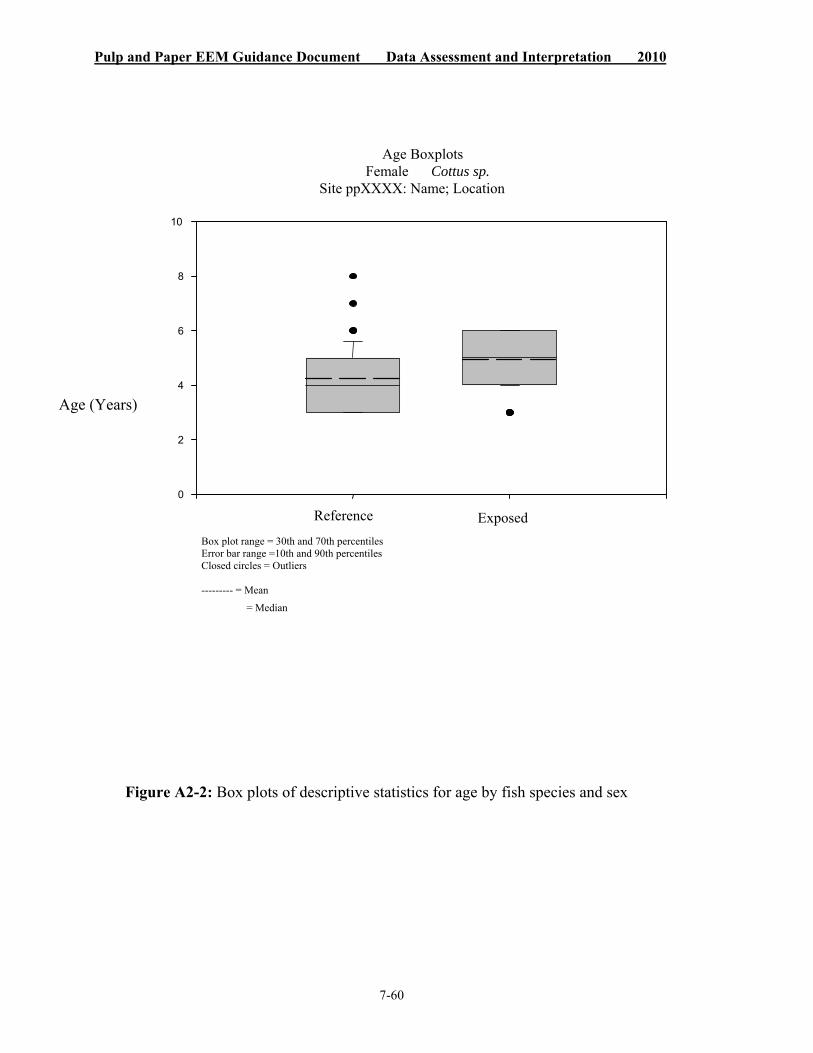
Pulp and Paper EEM Guidance Document Data Assessment and Interpretation 2010
10
8
6
4
Age (Years)
2
00 1 2 3Reference Exposed
--------- = Mean = Median
7-60
Age BoxplotsFemale Cottus sp.
Site ppXXXX: Name; Location
Box plot range = 30th and 70th percentilesError bar range =10th and 90th percentilesClosed circles = Outliers
Figure A2-2: Box plots of descriptive statistics for age by fish species and sex

Pulp and Paper EEM Guidance Document Data Assessment and Interpretation 2010
Figure 2: ppXXXX; Name; Location; Female Cottus sp. Age
Figure A2-3: Analysis of Variance (ANOVA) results of mean age of fish taken from reference and exposure areas (mean and standard error)
Note: Bars with different letters are significantly different. The vertical bar is a mean and the horizontal variance bars represent the standard errors.
Reference Exposure
Age
0
1
2
3
4
5
6
a
b
7-61

Pulp and Paper EEM Guidance Document Data Assessment and Interpretation 2010
3.13 2.92.6 2.7 2.8
1.4
1.2
1
0.6
0.8
7-62
Figure A2-4: Linear regression of fish liver weight at body weight as an example of effect summary for liver weight or gonad size – male Catostomus sp.
Log fish weight (Log10 g)
Log liver weight (Log10 g)
0.4
0.2
0
0.727
Linear
Linear (Exposed)
Referenc
Exposed
y = 1.2949x - 2.7088
y = 1.0296x - 1.8675 = 0.5135R 2
R2 =
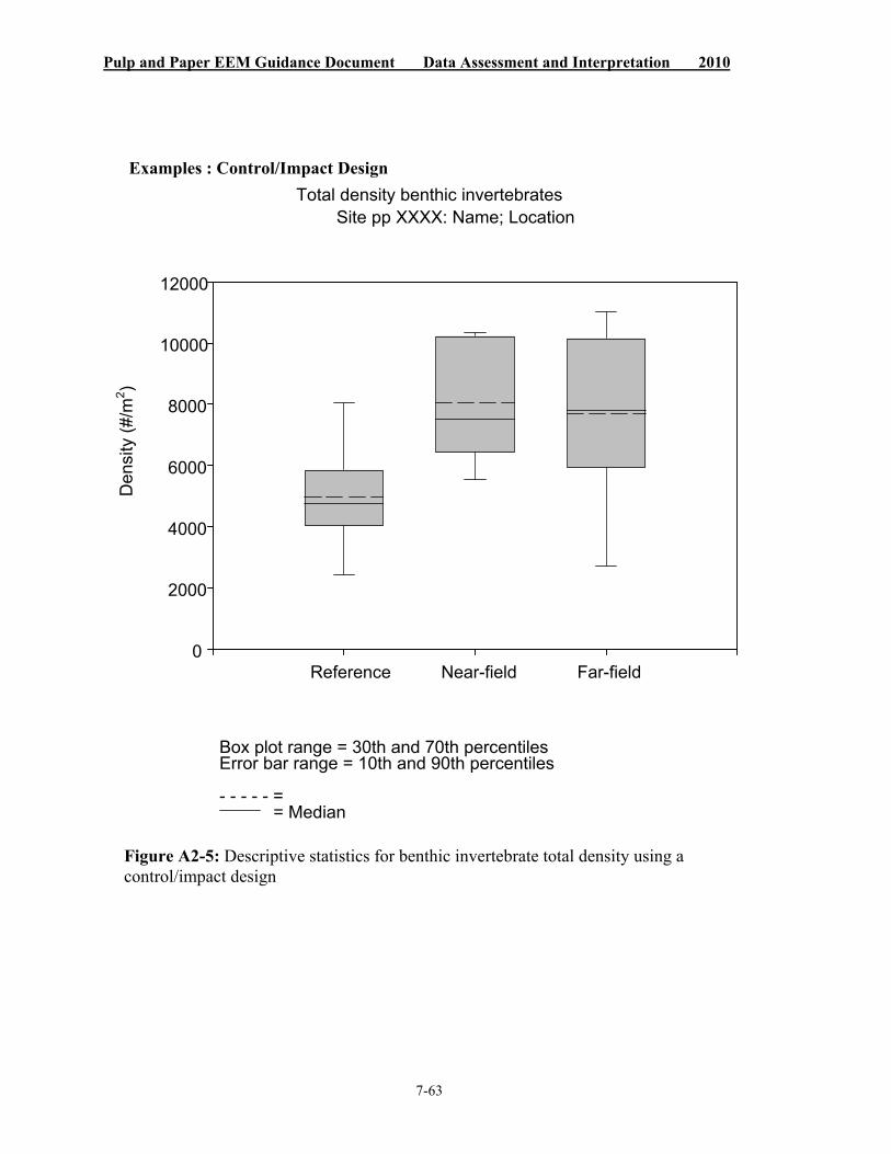
Pulp and Paper EEM Guidance Document Data Assessment and Interpretation 2010
12000
10000
Den
sity
(#/m
2 )
8000
6000
4000
2000
0 Reference Near-field Far-field
- - - - - = = Median
7-63
Examples : Control/Impact Design Total density benthic invertebrates
Site pp XXXX: Name; Location
Box plot range = 30th and 70th percentilesError bar range = 10th and 90th percentiles
Figure A2-5: Descriptive statistics for benthic invertebrate total density using a control/impact design

Pulp and Paper EEM Guidance Document Data Assessment and Interpretation 2010
Figure A2-6: Analysis of Variance (ANOVA) results of benthic invertebrate total density using a control/impact design
Note: Bars with the same letters are not significantly different. Values reported are means and associated standard errors.
20000
15000
, ±1
S.E
.) To
tal D
ensi
ty
aa2
10000
(num
ber/m
Reference Near-field Far-field0
5000
a
(Ref, n=5) (NF, (FF,
7-64
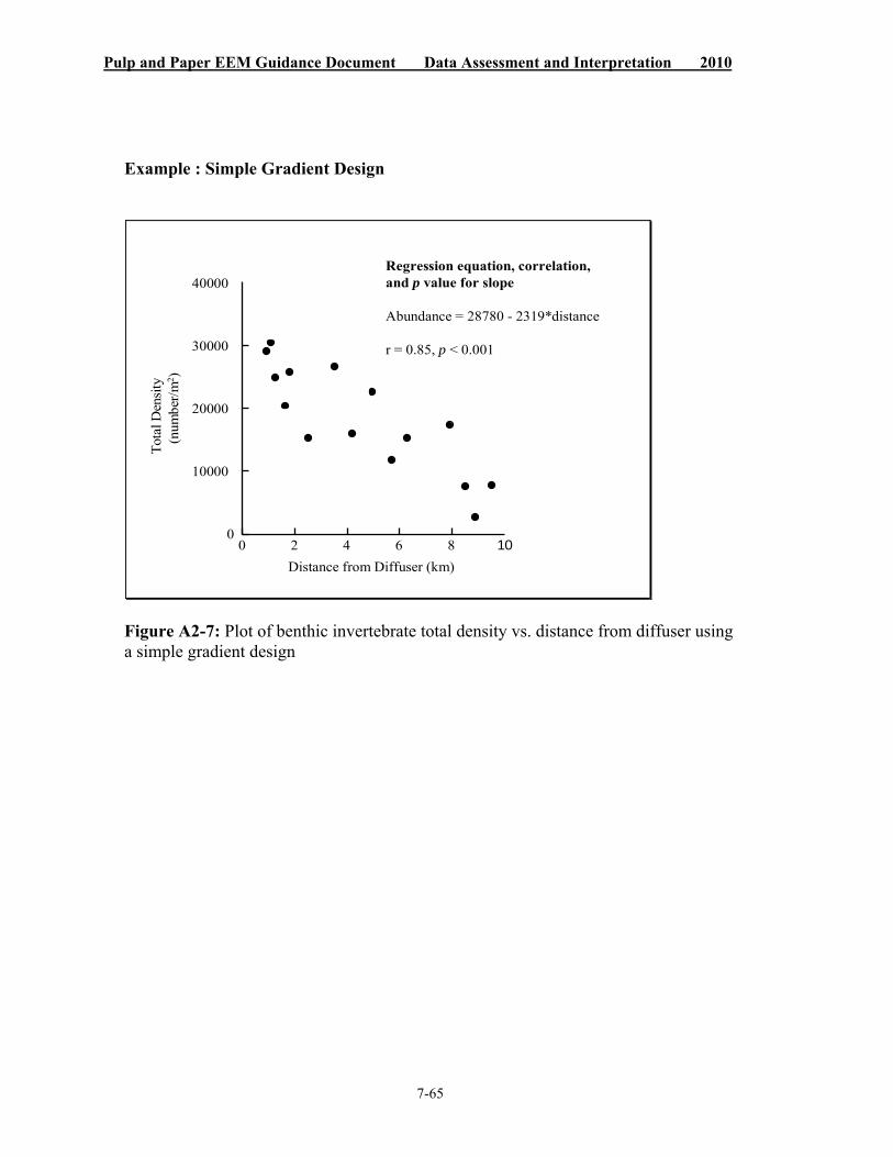
Example : Simple Gradient Design
Figure A2-7: Plot of benthic invertebrate total density vs. distance from diffuser usinga simple gradient design
Pulp and Paper EEM Guidance Document Data Assessment and Interpretation 2010
7-65
0 2 4 6 8 100
10000
20000
30000
40000
Tot
al D
ensi
ty(n
umbe
r/m
2 )
Regression equation, correlation,and p value for slope
Abundance = 28780 - 2319*distance
r = 0.85, p < 0.001
Distance from Diffuser (km)

Pulp and Paper EEM Guidance Document Data Assessment and Interpretation 2010
7-66
Table A2-1: Descriptive statistics for age by fish species and sex
Site ppXXXX: Name; Location Female Cottus sp. – Descriptive Statistics – Age
Location Mean SD* SE** (n) Max. Min.Reference 4.23 1.16 0.19 39 8.00 3.00
Exposure 4.93 0.93 0.14 46 6.00 3.00
* Standard deviation ** Standard error
Table A2-2: Analysis of Variance (ANOVA) results for fish age by species and sex
Site pp XXXX: Name; Location Female Cottus sp. – ANOVA Results – Age
Source of Variation Sum of Squares
(SS)
Degrees of freedom
(df)
Mean Square (MS)
F-Ratio p-value atsig. p < 0.05
Between groups 0.072624 1 0.072624 11.25004 0.001202 Yes Within groups 0.535802 83 0.006455 Total 0.608426 84

Pulp and Paper EEM Guidance Document Data Assessment and Interpretation 2010
Log-transformed Slopes Different? Log-transformed Means Different?
7-67
Table A2-3: Analysis of Covariance (ANCOVA) results for liver weight at body weight by sex and by species
Site: ppXXXX; Name; Location ANCOVA Results: Liver Weight at Body Weight – Male Catostomus sp.
Area N Slope SD R-Squared (R2)
(p-value) sig.at p < 0.05
Least Squares Means (LSM)
SD (p-value) sig. at p < 0.05
Antilog LSM Magnitude difference
Reference 39 1.3 0.0547 0.727 - - 0.95 0.0624 - - 8.93 - Exposure 38 1.03 0.0632 0.5135 0.212 no 1.04 0.0616 0.001 yes 10.96 23%

Pulp and Paper EEM Guidance Document Data Assessment and Interpretation 2010
7-68
Table A2-4: Fish result summary table
Site ppXXXX: Name; Location: Fish Effect Summary Trophic Level Species Sex Response Effect Endpoint Effect? Direction Magnitude
Fish Catostomus catostomus (Longnose Sucker)
F Survival Age NA
Energy Use Weight-at-age NA Relative gonad weight No
Energy Storage Condition Yes ref < exp 7%2 Relative liver weight Yes ref < exp 21%2
Catostomus catostomus (Longnose Sucker)
M Survival Age NA
Energy Use Weight-at-age NA Relative gonad weight NO
Energy Storage Condition Yes ref < exp 6%2 Relative liver weight Yes ref < exp 23%2
Cottus ricei (Spoonhead Sculpin)
F Survival Age Yes ref < exp 8%2
Energy Use Weight-at-age Yes ref < exp 52%1 Relative gonad weight Yes ref < exp 57%2
Energy Storage Condition Yes ref < exp 31%1 Relative liver weight Yes ref < exp 62%2
Cottus ricei (Spoonhead Sculpin)
M Survival Age Yes ref < exp 8%2
Energy Use Weight-at-age Yes ref < exp 106%1 Relative gonad weight Yes ref < exp 11%2
Energy Storage Condition Yes ref < exp 18%2 Relative liver weight Yes ref < exp 52%2
1 ANCOVA is done and the slopes are significantly different. See Appendix 1 for guidance on calculating magnitude of effect. 2 Magnitude calculated by comparing the adjusted means between reference and exposed sites (if data were log-transformed; magnitude is calculated on the antilog of the adjusted means). In this case, the slopes are not significantly different and so the adjusted means can be compared directly. (The equation is: [(exposed adjusted mean – reference adjusted mean)/ reference adjusted mean] x 100).

Pulp and Paper EEM Guidance Document Data Assessment and Interpretation 2010
7-69
Table A2-5: Descriptive statistics for total benthic invertebrate density (number of invertebrates/m2)
Site ppXXXX: Name; Location Descriptive Statistics – Benthic Invertebrate Density
Location Mean SD SE (n) Max. Min. Reference 4986.85 2011.21 899.44 5 8062.02 2442.73 Near-field 8062.73 2135.30 954.94 5 10360.31 5535.88 Far-field 7685.04 3205.63 1433.60 5 11027.65 2717.00
A2-6:Table Analysis of Variance (ANOVA) results for benthic invertebrate total density
Site ppXXXX: Name; Location ANOVA Results – Benthic Invertebrate Total Density
Source of Variation
SS df MS F p-value Sig. at p < 0.05
Between Groups 2.81E+07 2 1.41E+07 2.236 0.15 NOWithin Groups 7.55E+07 12 6.29E+06Total 1.04E+08 14

Pulp and Paper EEM Guidance Document Data Assessment and Interpretation 2010
7-70
Table A2-7: Summary of all benthic invertebrate descriptive statistics
Site:ppXXXX: Name; Location Effect Endpoint
Location Mean SD SE (n) Max. Min.
Taxa Ref 19.60 1.52 0.68 5 21 18
Near 21.20 1.48 0.66 5 23 19Field (NF)
Far Field 20.00 1.87 0.84 5 23 18(FF)
Density Ref 4986.85 2011.21 899.44 5 8062.02 2442.73NF 8062.73 2135.30 954.94 5 10360.31 5535.88FF 7685.04 3205.63 1433.60 5 11027.65 2717.00
Simpson’s Evenness Ref 0.77 0.03 0.014 5 0.82 0.75
NF 0.81 0.03 0.015 5 0.86 0.78FF 0.67 0.04 0.017 5 0.71 0.63
Bray-Curtis Ref 0.24 0.11 0.05 5 0.42 0.14NF 0.37 0.10 0.05 5 0.48 0.24FF 0.44 0.09 0.04 5 0.55 0.34
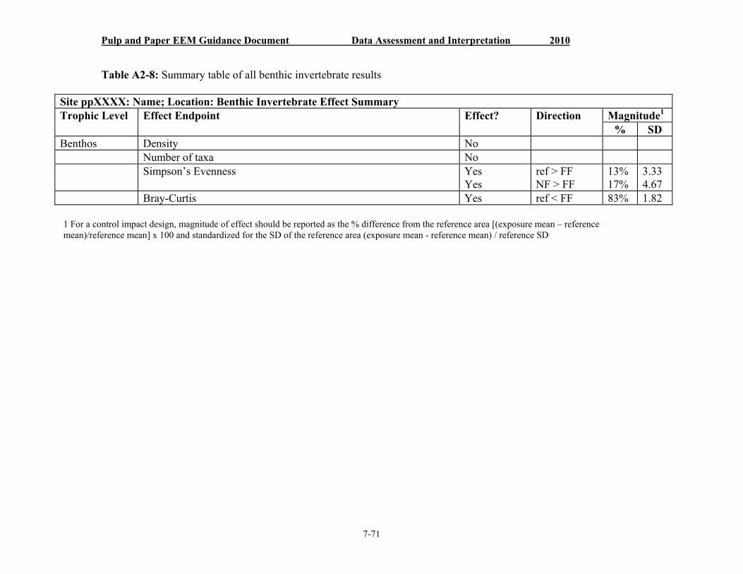
Pulp and Paper EEM Guidance Document Data Assessment and Interpretation 2010
7-71
Table A2-8: Summary table of all benthic invertebrate results
Site ppXXXX: Name; Location: Benthic Invertebrate Effect Summary Trophic Level Effect Endpoint Effect? Direction Magnitude1
% SD Benthos Density No
Number of taxa No Simpson’s Evenness Yes ref > FF 13% 3.33
Yes NF > FF 17% 4.67 Bray-Curtis Yes ref < FF 83% 1.82
1 For a control impact design, magnitude of effect should be reported as the % difference from the reference area [(exposure mean – reference mean)/reference mean] x 100 and standardized for the SD of the reference area (exposure mean - reference mean) / reference SD

Pulp and Paper EEM Guidance Document Data Assessment and Interpretation 2010
7-72
Table A2-9: Overall summary of site effects
Site ppXXXX: Name; Location: Site Effect Summary Trophic Level Species Sex Response Effect
Endpoint Effect? Direction Magnitude3
% SDFish Catostomus
catostomus (Longnose Sucker)
F Survival Age NA

Pulp and Paper EEM Guidance Document Data Assessment and Interpretation 2010
7-73
Energy use Weight-at-age NA Relative gonad weight
No
Energy storage Condition Yes ref < exp 7%2 Relative liver weight
Yes ref < exp 21%2
Catostomus catostomus (Longnose Sucker)
M Survival Age NA
Energy use Weight-at-age NA Relative gonad weight
No
Energy storage Condition Yes ref < exp 6%2 Relative liver weight
Yes ref < exp 23%2
Cottus ricei (Spoonhead Sculpin)
F Survival Age Yes ref < exp 8%2
Energy use Weight-at-age Yes ref < exp 52%1
Relative gonad weight
Yes ref < exp 57%2
Energy storage Condition Yes ref < exp 31%1
Relative liver weight
Yes ref < exp 62%2
Cottus ricei (Spoonhead Sculpin)
M Survival Age Yes ref < exp 8%2
Energy use Weight-at-age Yes ref < exp 106%1
Relative gonad weight
Yes ref < exp 11%2
Energy storage Condition Yes ref < exp 218%Relative liver weight
Yes ref < exp 52%2

Pulp and Paper EEM Guidance Document Data Assessment and Interpretation 2010
7-74
Benthos Density No Number of taxa
No
Simpson’s Yes ref > FF 13% 3.33 Evenness Yes NF > FF 17% 4.67
Bray-Curtis Yes ref < FF 83% 1.82 1 ANCOVA is done and the slopes are significantly different. See Appendix 1 for guidance on calculating magnitude of effect. 2 Magnitude calculated by comparing the adjusted means between reference and exposed sites (if data were log-transformed; magnitude is calculated on the antilog of the adjusted means). In this case, the slopes are not significantly different and so the adjusted means can be compared directly. (The equation is: [(exposed adjusted mean – reference adjusted mean)/ reference adjusted mean] x 100). 3 For benthic invertebrate community surveys following a control impact designs, magnitude of effect should be reported as the % difference from the reference area [(exposure mean – reference mean)/reference mean] x 100 and standardized for the SD of the reference area (exposure mean - reference mean) / reference SD

Pulp and Paper EEM Guidance Document Data Assessment and Interpretation 2010
7-75
Appendix 3 Case study – ANCOVA and Power Analysis for Fish Survey
A case example is provided to demonstrate the application of some of the methods recommended above. The data were collected during a previous adult fish survey at a Canadian pulp mill. In this particular example, the mill was a bleached-kraft operation and discharged effluent into a lake receiving environment. The reference area was an adjacent bay of the lake exhibiting similar natural habitat characteristics as the near-field area, and did not receive any allochthonous discharges. The sentinel fish species selected for the survey was White Sucker (Catastomus commersoni). The sample sizes approximated those recommended for the fish survey, with the exception of males at the near-field area:
Near-field area Reference area
Males 12 22
Females 26 24
The data set included information on length, weight, liver weight, sex, gonad weight, and age of male and female adult sucker. Fecundity estimates were not available.
After the initial step of ensuring the data set was free of transcription errors, the mean and standard deviation of each variable were calculated per sex and sampling area (Table A3-1). Mathematical procedures were conducted separately for males and females. Normal probability plots were generated for each variable (per sex and area) to identify extreme outliers and to assess normality of the data. Examination of these plots did not indicate obvious extreme outliers with the exception of one male from the near-field area. Residual plots from the Analysis of Variance (ANOVA) / ANCOVA models can also be used to inspect the data.

Pulp and Paper EEM Guidance Document Data Assessment and Interpretation 2010
7-76
Table A3-1: Mean, standard deviation (SD) and sample size (n) of measurements recorded on White Sucker (Catostomus commersoni) during the example survey
Sex Area Fork Length(cm)
Body Weight (g)
Gonad Weight
(g)
Liver Weight
(g)
Age (yr)
Female Reference 44.4±2.4 (24)
1135.1±150.4 (24)
46.0±7.5 (24)
15.8±2.1 (24)
10.8±3.4 (24)
Near-field 41.5±3.0 (26)
1081.7±228.4 (26)
36.9±15.9 (26)
17.8±7.5 (16)
11.1±3.0 (26)
Male Reference 41.4±1.8 (22)
975.9±90.1 (22)
66.4±11.1 (21)
10.8±1.6 (22)
10.5±3.0 (22)
Near-field 39.3±1.8 (12)
950.9±166.6 (11)
48.0±15.5 (12)
18.4±8.4 (12)
12.3±3.0 (12)
As previously outlined, most of the results were derived using ANCOVA. For the purposes of illustration, a detailed description is provided for the parameter size (length)-at-age for female White Sucker (one of the supporting endpoints for the fish survey). For these calculations, both length and age were log
10-transformed.
The first step is to conduct the preliminary test of equality of slopes. The model statement for this analysis of size-at-age is:
log(length) = constant + area + log(age) + area*log(age),
where the interaction term area*log(age) represents the test for equality of slopes of the area regression lines, and log(age) is the covariate. From the ANCOVA table, it is evident that the interaction term, area*log(age), is not significant (P=0.376) (Table A3-2a). This tells us that the slopes of the regression lines for each area can be treated as being approximately parallel. It also tells us that the interaction term can be dropped from the model, and we can proceed to the ANCOVA model:
log(length) = constant + area + log(age),
where area represents the test for differences in adjusted means. The mean square error (mean square error) from the resulting ANCOVA table will provide the estimate of

Pulp and Paper EEM Guidance Document Data Assessment and Interpretation 2010
7-77
variability (mean square error=0.00033) for length-at-age (Table 2b). While conducting the above analyses, the residuals from the preliminary and ANCOVA model can be saved for the purpose of assessing the assumptions of normality and homogeneity of variance.
Table A3-2: Size-at-age (log(length) vs log(age)) for female White Sucker using ANCOVA. The analysis includes: a) a preliminary test of the equality of slopes, and (b) the ANCOVA model table (test of adjusted means)
(a) Preliminary Analysis of Equality of Slopes
Source Sum-of-Squares(SS)
Degrees of Freedom (df)
Mean-Square (MS)
F-Ratio p-Value
Area 0.00086 1 0.00086 2.62639 0.11193
Log(age) 0.02126 1 0.02126 64.58474 < 0.0001
Area*Log(age) 0.00026 1 0.00026 0.79780 0.37640
Error 0.01514 46 0.00033
(b) ANCOVA Model
Source SS df MS F-Ratio p-value
Area 0.01240 1 0.01240 37.57576 < 0.0001
Log(age) 0.02167 1 0.02167 65.66667 < 0.0001
Error 0.01541 47 0.00033
Calculation of Sample Size
To calculate sample size, the Z-value power equation described earlier can be used. As a reminder, the equation is:
n = 2 (Z + Z)2 (SD/CES)2 + 0.25Z2

Pulp and Paper EEM Guidance Document Data Assessment and Interpretation 2010
7-78
The square root of the mean square error from the ANCOVA model substitutes for the SD in the power equation. The critical effect size (CES) refers to the effect or difference in the parameter one wishes to detect. For the purpose of this example and the remaining parameters of the case study, samples sizes were calculated for a CES of 5, 10, 20, 50 and 100% (i.e., differences between areas).
Many of the parameters calculated for the fish survey, are typically log-normally distributed and require log transformations. To calculate sample sizes, SD and CES should be expressed in logarithms. It should be noted, however, not to add 1 to values before logging for the purposes of the fish environmental effects monitoring (EEM) survey because it has undesirable effects on the calculated variances when changing measurement units. A difference in logarithms is equivalent to multiplying or dividing by some factor. For example, if the difference in log length between two areas is 0.301, then the fish from one area is twice the length (antilog 0.301 = 2) as fish from the other area. In the following table, CES has been expressed in logarithms with the corresponding antilog; these values of CES correspond roughly with those used for untransformed data:
Critical effect size
(logarithm)
0.0212
0.0414
0.0792
0.176
0.301
Critical effect size
(antilog)
1.05
1.10
1.20
1.50
2.00
% increase*
5
10
20
50
100
% decrease†
5
9
17
33
50
Therefore for length-at-age (log10 data):
SD = (mean square error)0.5 = (0.00033)0.5 = 0.01817 Z(2) (2-tailed test)= 1.96
Z (1-tailed test) = 1.282 CES = 5% (see above table)
n = 2 (1.96+1.28)2 (0.01817/0.0212)2 + 0.25(1.96)2
n = 16.4 (or, rounding up, n=17)
Similarly for the remaining effect sizes, the estimated sample sizes (i.e., number of fish to be sampled per area) would be:
* In exposure area vs reference † In exposure area vs reference

Pulp and Paper EEM Guidance Document Data Assessment and Interpretation 2010
7-79
CES 5% 10% 20% 50%
n 17 5 3 2
The estimate of variability and sample size calculations for gonad weight, liver weight and condition for female and male sucker were calculated in the same fashion as described for length-at-age (Table 4). In all but one case, the slopes of the reference/near-field regression lines were equal and the mean square errors from the ANCOVA model were used as the estimate of variability. For male White Sucker, the slopes of the regressions of log(weight) on log(length) (i.e., condition) were not equal among areas (P=0.0068). To investigate whether the one possible outlier (male, near-field) influenced the ANCOVA, it was rerun without this data point. In this case, the regressions were homogeneous between areas. This was partially a consequence of the low sample size (i.e., an increased influence of an outlier on the regression) and should be noted when reporting the data.
For mean age, the mean square error from the one-way ANOVA was used to estimate the variability (Table 4).
The final results of the sample size calculations (Table 4) indicate that the maximum numbers of fish needed to be collected from each area were approximately 703 males and 738 females to detect a 5% difference between areas (CES), 185 males and 194 females to detect a 10% difference, 52 males and 54 females to detect a 20% difference, and 12 males and 12 females to detect a 50% difference. Among all the parameters, mean age was the most variable and required the highest sample size to detect differences.

Pulp and Paper EEM Guidance Document Data Assessment and Interpretation 2010
7-80
Estimated Sample Size (number of fish/area)
Table A3-3. Numbers of fish needed to detect significant differences in fish endpoints among areas using the model mean square error as the estimate of variability. Sample sizes were calculated for a range of CESs with power=0.90 and =0.05. All data were log
10-transformed – example survey
Endpoint Sex Model Log
MeanSquare Error
CES=5%
CES=10%
CES=20%
CES= 50%
Length-at-age Male ANCOVA 0.00014 8 3 2 2
Female ANCOVA 0.00033 17 5 3 2
Weight-at-age Male ANCOVA 0.00211 100 27 9 3
Female ANCOVA 0.00295 139 38 11 3
Condition Male 1ANCOVA N/A - - -
-
Female ANCOVA 0.00100 48 14 5 2
Liver Weight Male ANCOVA 0.00994 466 123 35 8
Female ANCOVA 0.00626 294 78 22 6
Gonad Weight Male ANCOVA 0.00881 413 110 31 7
Female ANCOVA 0.01013 475 126 35 8
Mean Age Male ANOVA 0.01499 703 185 52 12
Female ANOVA 0.01574 738 194 54 12
1 Preliminary analysis (test of slopes) conducted as first step to ANCOVA was significant (i.e., slopes not parallel).

Pulp and Paper EEM Guidance Document Alternative Monitoring Methods 2010
8-I
Table of Contents
8. Alternative Monitoring Methods ......................................................................................... 8-1 8.1 Overview...................................................................................................................... 8-1 8.2 Use of Mesocosms as an Alternative Monitoring Method .......................................... 8-2
8.2.1 Background Information on Artificial Stream Development and Application........ 8-2 8.2.2 Applicability within the EEM Programs................................................................ 8-27 8.2.3 Mesocosm Technology .......................................................................................... 8-27
8.2.3.1 Suitability of Mesocosm Design.................................................................... 8-27 8.2.3.2 Description and General Operation of Large Trailer Mesocosm System...... 8-28 8.2.3.3 Description and General Operation of Modular Mesocosm System ............. 8-29
8.2.4 Considerations for Site Selection........................................................................... 8-30 8.2.5 Biological Monitoring Study Designs ................................................................... 8-31
8.2.5.1 Overview........................................................................................................ 8-31 8.2.5.2 Study Treatments ........................................................................................... 8-32 8.2.5.3 Replication ..................................................................................................... 8-33 8.2.5.4 Sample Sizes and the Role of Effect Size...................................................... 8-33
8.2.5.4.1 No Available Pre-existing (Historical) Data.............................................. 8-33 8.2.5.4.2 Available Pre-existing (Historical) Data.................................................... 8-34
8.2.6 Fish Monitoring – Effects Assessment .................................................................. 8-35 8.2.6.1 Study Design.................................................................................................. 8-35
8.2.6.1.1 Species Selection ....................................................................................... 8-35 8.2.6.1.2 Effect Indicators......................................................................................... 8-37 8.2.6.1.3 Timing and Duration of Effluent Exposure ............................................... 8-42
8.2.6.2 Fish Methods.................................................................................................. 8-43 8.2.6.2.1 General Set-up – Trailer Mesocosm System ............................................. 8-43 8.2.6.2.2 General Set-up – Modular Mesocosm System........................................... 8-44 8.2.6.2.3 Maintenance and Monitoring..................................................................... 8-45 8.2.6.2.4 Sampling and Analysis of Fish .................................................................. 8-46
8.2.6.3 Data Assessment and Interpretation............................................................... 8-46 8.2.6.3.1 General Requirements................................................................................ 8-46 8.2.6.3.2 Statistical Analysis of Parameters.............................................................. 8-47 8.2.6.3.3 Nested ANOVA Analyses ......................................................................... 8-47 8.2.6.3.4 ANCOVA Analyses................................................................................... 8-47 8.2.6.3.5 Data QA/QC and Analysis......................................................................... 8-48
8.2.7 Benthic Invertebrate Community Monitoring - Effects Assessment..................... 8-48 8.2.7.1 Study Design.................................................................................................. 8-48
8.2.7.1.1 Species Selection ....................................................................................... 8-48 8.2.7.1.2 Effect Endpoints......................................................................................... 8-48 8.2.7.1.3 Timing and Duration of Effluent Exposure ............................................... 8-48
8.2.7.2 Benthic Invertebrate Methods........................................................................ 8-49 8.2.7.2.1 Mesocosm Trailer – General Set-up .......................................................... 8-49 8.2.7.2.2 Modular Mesocosm – General Set-up ....................................................... 8-50 8.2.7.2.3 Maintenance and Monitoring..................................................................... 8-51
8.2.7.3 Sampling and Analysis of Benthic Invertebrates........................................... 8-51 8.2.7.4 Data Assessment and Interpretation............................................................... 8-52

Pulp and Paper EEM Guidance Document Alternative Monitoring Methods 2010
8-II
8.2.8 Supporting Measurements ..................................................................................... 8-53 8.2.8.1 Water Chemistry Parameters ......................................................................... 8-53 8.2.8.2 Supporting Water Quality Parameters ........................................................... 8-53
8.3 Use of Caged Bivalves as an Alternative Monitoring Method.................................. 8-54 8.3.1 Introduction............................................................................................................ 8-54 8.3.2 Background............................................................................................................ 8-54 8.3.3 Approach................................................................................................................ 8-55 8.3.4 Species Selection ................................................................................................... 8-58
8.3.4.1 Most Commonly Used Taxa .......................................................................... 8-58 8.3.4.2 Marine and Estuarine Bivalves ...................................................................... 8-60 8.3.4.3 Freshwater Bivalves....................................................................................... 8-61 8.3.4.4 Source ............................................................................................................ 8-62 8.3.4.5 Species Identification..................................................................................... 8-63 8.3.4.6 Size and Age .................................................................................................. 8-64 8.3.4.7 Number of Organisms.................................................................................... 8-65 8.3.4.8 Handling and Holding Conditions ................................................................. 8-65
8.3.5 Study Design.......................................................................................................... 8-65 8.3.5.1 Sampling Design............................................................................................ 8-66
8.3.5.1.1 Area and Station Selection......................................................................... 8-67 8.3.5.2 Replication ..................................................................................................... 8-67
8.3.5.2.1 Number of Cage Stations ........................................................................... 8-67 8.3.5.2.2 Applying Replication to Study Design ...................................................... 8-68
8.3.5.3 Timing and Duration...................................................................................... 8-68 8.3.5.4 Modifying or Confounding Factors and Supplementary Measures............... 8-69
8.3.6 Cage Designs ......................................................................................................... 8-69 8.3.6.1 Mooring Systems ........................................................................................... 8-69
8.3.7 Methods for Test Initiation, Cage Deployment and Retrieval and Test Termination8-72
8.3.7.1 Test Initiation ................................................................................................. 8-72 8.3.7.2 Cage Deployment........................................................................................... 8-73 8.3.7.3 Cage Retrieval and Test Termination ............................................................ 8-73
8.3.8 Effect Indicators..................................................................................................... 8-74 8.3.8.1 Survival .......................................................................................................... 8-75 8.3.8.2 Growth ........................................................................................................... 8-75 8.3.8.3 Condition........................................................................................................ 8-75 8.3.8.4 Energy Measure ............................................................................................. 8-76 8.3.8.5 Reproductive Effort ....................................................................................... 8-77
8.3.9 Quality Assurance and Quality Control................................................................. 8-79 8.3.10 Data Analyses .................................................................................................... 8-80 8.3.11 Dioxins and Furans ............................................................................................ 8-81 8.3.12 Reporting............................................................................................................ 8-81
8.4 References.................................................................................................................. 8-81

Pulp and Paper EEM Guidance Document Alternative Monitoring Methods 2010
8-III
List of Tables
Table 8-1: Summary of artificial stream applications for assessing the effects of pulp and paper and mining effluents on aquatic ecosystems as required under Canadian environmental effects monitoring ................................................................................................................ 8-4
Table 8-2: Fish mesocosm study effect indicators and endpoints and related statistical procedures............................................................................................................................................ 8-37
Table 8-3: Recommended (shaded) response variables and suitable additional supporting information, and suggested statistical analysis for Fathead Minnow application in modular mesocosm systems ............................................................................................................. 8-39
Table 8-4: Suggested taxa for use in caged bivalve studies for EEMs...................................... 8-59 Table 8-5: Differences noted between two species of mussels over 5-year study in the Burrard
Inlet, Vancouver, British Columbia ................................................................................... 8-61 Table 8-6: Differences noted between Unionoidea and Sphaeriidae......................................... 8-62 Table 8-7: Caged bivalve study effect indicators and endpoints and related statistical procedures
............................................................................................................................................ 8-74 Table 8-8: An example of a field data sheet for recording survival and growth raw data*....... 8-78
List of Figures Figure 8-1: A) Large mesocosm system with streams situated on tables (Model I) used in the
Athabasca River, Alberta. B) Large mobile mesocosm system with streams on 2 trailers (Model II) used in the Fraser River, British Columbia; the Saint John River, New Brunswick; and in Saint John Harbour, New Brunswick. C) Large mobile mesocosm system with streams on a single trailer (Model III) used in the Miramichi and Little rivers, New Brunswick; the Wapiti River, Alberta; and Junction Creek, Ontario ................................ 8-18
Figure 8-2: A) Small microcosm system with streams situated on tables over mixing reservoirs used in the Thompson River, British Columbia. B) Modular mesocosm system with streams situated on tables over mixing reservoirs used in the Little River, New Brunswick; Junction Creek, Ontario; the Wabigoon River, Ontario; and Key Lake, Saskatchewan.................. 8-19
Figure 8-4: Photograph of a modular mesocosm set-up ............................................................ 8-21 Figure 8-5: Modular mesocosm flow schematic........................................................................ 8-22 Figure 8-6: Multitrophic Fathead Minnow reproductive bioassay and feeding barrier............. 8-23 Figure 8-7: Site set-up for modular mesocosms ........................................................................ 8-24 Figure 8-8: A) Factorial experimental design to investigate the importance of water vs. diet in
responses of Fathead Minnow to metal mine effluent in modular mesocosms; B) Experimental design to investigate the influence of pH and natural organic matter (NOM) on Fathead Minnow responses after exposure to an MME mixture and a single metal in multitrophic modular mesocosms ...................................................................................... 8-25
Figure 8-9: Factorial experimental design to investigate the effects of MME and historical sediment contamination in isolation and in combination on Fathead Minnow in modular mesocosms. ........................................................................................................................ 8-26
Figure 8-10: Mussel showing ripe mantle lobe.......................................................................... 8-56 Figure 8-11: Reproductive cycle of Blue Mussels from British Columbia: A) Mantle energy
stored in fall; B) Mantle reproductive content in spring.................................................... 8-57 Figure 8-12: Mytilus spp. shell scars markings.......................................................................... 8-64

Pulp and Paper EEM Guidance Document Alternative Monitoring Methods 2010
8-IV
Figure 8-13: Duplicate frame from a caged mussels exposure experiment............................... 8-70 Figure 8-14: Modular mesocosm parts diagram ........................................................................ 8-71 Figure 8-15: Modular mesocosm flow schematic...................................................................... 8-72 Figure 8-16: A) Mantle plug and tools necessary for its removal; B) Mantle plug after
homogenization and ready for assessment......................................................................... 8-77

Pulp and Paper EEM Guidance Document Alternative Monitoring Methods 2010
8-1
8. Alternative Monitoring Methods
8.1 Overview
At some mills, standard fish and benthic invertebrate community monitoring studies may not be appropriate. The reasons for this are site-specific, but the most common reasons are the presence of hazardous conditions (e.g., high flow velocity); unsuitable habitat for sampling; or the presence of confounding factors, such as other effluent discharges in the exposure area, that make it impossible to isolate any effects attributable to the effluent being monitored.
Where mills cannot design the fish or benthic invertebrate community surveys to resolve difficulties associated with confounding influences, they will provide a scientific rationale and justification, and propose cost-effective and technically feasible alternative monitoring methods within the study design. A number of alternative monitoring methods are recommended in this chapter.
Mills may choose other scientifically defensible methods, provided that the results can determine if the effluent is having effects on the fish population (growth, reproduction, condition and survival), fish tissue (dioxins and furans), or the benthic invertebrate community (benthic invertebrate density, taxa richness, the Simpson’s Evenness Index and the Bray-Curtis Index). Currently, recommended alternatives to the fish survey monitoring method are mesocosm (artificial stream) and caged bivalve studies. For benthic invertebrate community surveys, the recommended alternative monitoring method is the mesocosm study.
Other alternatives to the fish and benthos field surveys may also exist. Mills can suggest other alternative methods in their study design. New alternative methods will be evaluated by the Authorization Officer, with the support of the Technical Advisory Committee and the Environmental Effects Monitoring (EEM) Science Committee. In reviewing the suggested alternative, some specific design elements will be considered as essential to meeting the objective of the program, including environmental relevance and interpretable results that are scientifically defensible and manageable.
The objective of section 8.2 is to provide guidance on the study design and implementation of mesocosm studies as an alternative EEM method for assessing the effects of pulp mill effluent on benthic invertebrates and fish. This guidance document is intended to provide information on recommended standards of good scientific practice available to meet the outlined EEM requirements. In 2005, the first guidance document for the use of artificial stream systems (mesocosms) was released. Guidance was updated in 2009 to reflect ongoing research and development for improvement of this alternative EEM method.
The objective of section 8.3 is to provide technical guidance for conducting controlled experiments using caged bivalves suspended in the water column to test for effects associated with industrial discharges and to compare measurements between exposure and reference areas. Caged bivalves are also an alternative to the fish survey and may be considered for mills where the fish survey has been unsuccessful or impractical in past cycles of EEM, or where there may be study design issues, such as confounding influences, or safety concerns.

Pulp and Paper EEM Guidance Document Alternative Monitoring Methods 2010
8-2
8.2 Use of Mesocosms as an Alternative Monitoring Method
8.2.1 Background Information on Artificial Stream Development and Application
Artificial streams are recommended as monitoring alternatives because years of research and development have demonstrated that, with respect to effluent effects, they can produce good-quality data that fit within the required regulatory context (Table 8-1). Since 1991, field-based artificial stream system studies have been conducted for assessing the effects of point-source effluents on aquatic ecosystems. Field-based artificial stream studies relevant to EEM applications were conducted in Canada 14 times in 8 years between 1993 and 2008 (Table 8-1). All of these studies, and development of the alternative method, were conducted as collaborative partnerships between industry, government, academia and consultants. All funding for the research was acquired through mechanisms independent of the EEM Program. Applications of this method are presented in detail below to provide a thorough understanding of the work that has been done to date. A summarized version with references can be found in Table 8-1. These references should be consulted if similar types of studies and experimental designs are being considered.
1991-1996, Northern River Basins Study (NRBS), Alberta
One of the first mesocosm applications assessed the effects of pulp mill effluent (PME) on benthic invertebrate and periphytic algal communities in the Athabasca River (Table 8-1) (Culp and Podemski 1996; Culp et al. 1996; Podemski and Culp 1996; Podemski 1999; Culp et al. 2001). Artificial streams were used to distinguish the effects of nutrients in whole mill effluent from contaminants, on the basis of directional differences in biological response. Specifically, moderate nutrient enrichment would increase primary and secondary productivity, whereas contaminant effects would reduce growth and reproduction and eventually result in mortality (Culp and Podemski 1996; Podemski and Culp 1996; Culp and Lowell 1998; Culp et al. 2001). To achieve this objective, 3 treatments were tested in the spring of 1993: control Athabasca River water, 1% (volume/volume [v/v]) treated PME, and 1% (v/v) nutrients (nitrogen + phosphorus) at levels measured in the PME. The hypothesis was that exposure to both the PME and nutrient treatments would result in nutrient enhancement effects on the benthic food web and that the PME and nutrient treatments would not differ. This would suggest that the effects of PME at levels found in the Athabasca River were due to nutrient enrichment rather than contaminant toxicity.
A large non-mobile artificial stream system was used near the pulp mill at Hinton, Alberta. The system consisted of 16 circular tanks or streams (0.9 m2 each) placed on tables (Model I, Figure 8-1A). River water was pumped into each stream at a controlled rate, and effluents and nutrients were added to the treatment streams as previously published by Culp and Podemski (1996) and Podemski (1999). A standardized benthic community, endemic to the Athabasca River, was created in each stream and exposed to PME for 28 days. At the end of the exposure period, algal biomass, growth of mayfly (Ephemeroptera: Siphloneuridae, Baetidae) and stonefly (Plecotera: Capniidae) nymphs, and insect abundance, increased in the treatment streams relative

Pulp and Paper EEM Guidance Document Alternative Monitoring Methods 2010
8-3
to the reference treatment (Culp and Podemski 1996; Podemski and Culp 1996; Culp et al. 1996). In addition, these response variables did not differ between the 1% PME and the 1% nutrient treatments, supporting the hypothesis that the effects of PME on the benthic food web were attributable to nutrient enrichment.
1991-1998, Fraser River Action Plan (FRAP), British Columbia
The FRAP was conducted from 1991 to 1997 to determine the current state of health of the Fraser River Basin ecosystem, including assessment of 8 pulp and paper mill effluents (Gray and Tuominen 1998; McGreer and Belzer 1998).
Thompson River, Kamloops, British Columbia (1993-1994)
The Thompson River showed signs of nutrient enrichment due to the discharge of PME at the City of Kamloops. This problem has been investigated since the early 1970s, when excessive accumulations of periphytic algae occurred in the river downstream of the pulp mill (Federal-Provincial Thompson River Task Force 1976). Bothwell and Daley (1981), Bothwell (1985), Bothwell et al. (1992) and Bothwell and Culp (1993) illustrated how periphytic algae growth was enriched by bioavailable phosphorus discharged in PME.
Artificial streams were used to separate the interacting effects of nutrients and contaminants in PME on algae and benthic invertebrates (Table 8-1). The approach differed from the NRBS studies in that a dose-response design was employed with the expectation of observing nutrient effects at low effluent concentrations and contaminant effects at higher concentrations. In 1993 and 1994, periphytic algae and chironomids were exposed to a dilution series of PME (0.25-10% [v/v]) (Dubé and Culp 1996; Culp and Lowell 1998). Smaller artificial streams were used for testing the effects of the PME on single insect species (Lowell et al. 1995, 1996) and simplified benthic food webs (Dubé and Culp 1996). The single-species approach focused the assessment of effects on key sentinel taxa, to improve our understanding of species-specific responses (Culp et al. 2000b).
The artificial stream system was set up on the banks of the Thompson River at Kamloops just upstream of the effluent outfall. The system included a water distribution system, treatment reservoirs for mixing the respective effluent dilutions with a continuous supply of river water, and small circular 0.33-L streams (45 cm2 planar area) (Dubé 1995; Lowell et al. 1995) (Figure 8-2A). Algae and chironomid larvae (Diptera: Orthocladiinae) from a reference area were placed into the streams, and changes in algae and chironomid biomass were measured after 2-3 weeks of effluent exposure (Dubé and Culp 1996). Dubé and Culp (1996) reported that algal biomass (chlorophyll a) increased in all effluent concentrations due to nutrient enrichment. Total chironomid biomass and individual weight were also enriched at low effluent concentrations (< 5%). At higher concentrations (5% and 10%) chironomid biomass decreased, possibly due to contaminant effects.

Pulp and Paper EEM Guidance Document Alternative Monitoring Methods 2010
8-4
Table 8-1: Summary of artificial stream applications for assessing the effects of pulp and paper and mining effluents on aquatic ecosystems as required under Canadian environmental effects monitoring
Year Program1 Effluent 2 ypeT
e Research Objectiv Location lArtificia Stream System
References
1993-1994
NRBS PME To determine the effect of nutrients and contaminants in PME on periphytic algae and benthic invertebrate communities
Athabasca veRi r,
Hinton, AB
Model I: Large non-emobile m socosm.
Benthos. Field study.
Podemski (1999) Culp and Podemski (1996) Podemski and Culp (1996) Culp et al. (1996) Culp et al. (2001)
1993-1994
FRAP PME To assess the effects of s increasing concentration of
n peripPME (0.25–10%) o n hyto:and chironomids (Diptera
Orthocladiinae)
hoT mpson River, Kamloops,
C B
all micSm rocosm system. Benthos. Field study.
995) Dubé (1Dubé and Culp (1996) Dubé et al. (1997)
ll et al. (2000) Lowe
1993 FRAP PME To determine the food-dependent effects of PME on the mayfly species Blue-winged Olive (Ephemeroptera: Baetis tricaudatus)
hoT mpson River, Kamloops, BC
mall micS rocosm system. Benthos. Field study.
well et al. (1995) Loll et al. (1996) Lowe
Culp et al. (1996) Lowell et al. (2000)
1994 FRAP ME P To determine the effects of PME hyto(1% and 3%) on perip n and
benthic invertebrate communities
F asr er River, rincP e eorG ge, BC
Model II: Large mobile mesocosm.
s. Field study. Bentho
Culp and Cash (1995) Culp et al. (1996) Culp et al. (2000a)
1997 Pulp and Paper EEM
PME To assess the effects of PME (3%) on a small-bodied fish, Mummichog (Fundulus heteroclitus), in a marine environment
Saint John Harbour,
aintS John, NB
Model II: Large mobile mesocosm.
. FieldFish study.
Cash et al. (2002)
1997-1998
Pulp and Paper EEM
PME To determine the effects of final s streams, PME, in-mill proces
and a mill process change on a small-bodied fish, Mummichog, in an estuarine environment
Saint John River, Saint John, NB
Model II: Large mobile mesocosm. Fish. Field study.
Dubé (2000) Dubé and MacLatchy (2000) Cash et al. (2002)

8-5
Year Program1 Effluent Type2
Research Objective Location Artificial Stream System
References
Pulp and Paper EEM Guidance Document Alternative Monitoring Methods 2010
1999 TSRI PME To determine the effects of primary- and secondary-treated PME on a small-bodied fish, Mummichog, in an estuarine environment
iraM michi iveR r,
Miramichi, NB
Model III: Large mobile mesocosm. Fish. Field study.
Dubé et al. (2002)
2000 TSRI MME To determine the effects of MME (20%, 80%) on juvenile Atlantic Salmon (Salmo salar)
ittlL e River, Brunswick Mines, Miramichi, NB
Model III: Large esocosm. mobile m
Fish. Field study.
Dubé et al. (2005)
2001 TSRI ME PMSE
ual To evaluate the individ and combined impacts of MSE and
e PME on Longnose Dac) (Rhinichthys cataractae
Wapiti River, AB
Model III: Large esocosm. mobile m
Fish. Field study.
Dubé et al. (2004)
2001 TSRI PME MSE
ual To evaluate the individ and f MSEcombined impacts o and
ic food PME on the benth web
apW iti River, Grande Prairie, AB
I: Large Model IIle memobi socosm.
s. Field study. Bentho
Culp et al. (2004)
2001-2002
Industry MME To assess effects of treated MMEs from three mines discharging to Junction Creek, Sudbury, on Creek Chub (Semotilus atromaculatus) and Pearl Dace (Semotilus margarita)
Junction Creek, Sudbury, ON
Model III: Large mobile mesocosm. Fish. Field study.
Dubé et al. (2006)
2002 Industry MME To evaluate the effects of MME l life cy(45%) on the partia cle of
omthe chironomid Chiron us tentans
Junction Creek,
bSud ury, ON
Modular mesocosm system. Benthos. Field study.
Hruska and Dubé (2004)
2003 NSERC MME Comparison of a partial–life-cycle bioassay in artificial streams to a standard beaker bioassay, to assess effects of
Junction Creek, Sudbury, ON
Modular mesocosm system. Benthos. Lab study.
Hruska and Dubé (2005)

Year Program1 Effluent Type2
Research Objective Location Artificial Stream System
References
8-6
Pulp and Paper EEM Guidance Document Alternative Monitoring Methods 2010
MME (45%) on the chironomid C. tentans
2003 NSERC/ Industry
PME To determine effects of final PME (1%, 100%) and various process streams on the partial life cycle of Fathead Minnow (Pimephales promelas) under environmentally realistic conditions (i.e., ambient water and effluent quality)
rTer ace Bay, ON
tBioassay railer. Fish. Field study.
Rickwood et al. (2006a, 2006b)
2004 C/ NSERIndustry
MME ninTo develop a self-sustai g , using multitrophic bioassay C.
nnow tentans and Fathead Mi(partial life cycle) to
fects of comparatively assess efd- and water-borne vs. foo
water- e to Mborne exposur ME now(45%) on Fathead Min
reproduction
cJun tion Creek, Sudbury, ON
esocosmModular m system. Multitrophic. Lab study.
Rickwood et al. (2006c)
2005 NSERC/ Industry
MME taininTo develop a self-sus g multitrophic bioassay, using C.
d Minnow tentans and Fathea(partial life cycle) to
s effects of comparatively assesorne vs. food- and water-b
water-borne exposure to MME ow(45%) on Fathead Minn
reproduction
Junction Creek, Sudbury, ON
Modular mesocosm system. Multitrophic. Field study.
Rickwood et al. (2008)
2006 NSERC/ Industry
PME To assess effects of PME (20%, 40%, 60%) on Fathead Minnow (partial life cycle)
Wabigoon River, Dryden, ON
Modular mesocosm system. Fish. Field study.
Pollock et al. (2009)

Pulp and Paper EEM Guidance Document Alternative Monitoring Methods 2010
8-7
Year Program1 Effluent Type2
Research Objective Location Artificial Stream System
References
2007 NSERC/ Industry
MME and
tpoten ial causative metal
To comparatively evaluate response patterns of Fathead Minnow (partial life cycle) to an MME mixture (100%, 25%, 5%) vs. selenium as selenate, using a multitrophic mesocosm bioassay
Unknown akeL , Key
Lake, SK
Modular mesocosm . Fish. Lab system
study
Pollock et al. (unpublished)
2008 NSERC/ Industry
MME To comparatively evaluate ischargeeffluent (current d : 25%)
l vs. sediment (historicare contamination) exposu
pathways on Fathead Minnow (partial life cycle)
nkU nown Lake, Key Lake, SK
Modular mesocosm system. Fish. Field study.
Driessnack et al. (unpublished)
2008 NSERC/ Industry
MME To assess the effects of three different MME discharges on Fathead Minnow (partial life cycle).
Junction Creek, Sudbury, ON
Modular mesocosm system. Multitrophic. Field study.
Ramilo et al. (unpublished)
1 NRBS: Northern River Basins Study; FRAP: Fraser River Action Plan; EEM: Environmental Effects Monitoring; TSRI: Toxic Substances Research Initiative; NSERC: Natural Sciences and Engineering Research Council of Canada. 2PME: pulp mill effluent; MSE: municipal sewage effluent; MME: metal mine effluent.

Pulp and Paper EEM Guidance Document Alternative Monitoring Methods 2010
8-8
In 1993, Lowell et al. (1995, 1996) conducted small-scale artificial stream experiments on the Thompson River in concert with those of Dubé and Culp (1996). Using the mayfly species Blue-winged Olive, the effects of PME (1% and 10% v/v) on survival, growth, moulting and morphological development were investigated under 2 feeding regimes (low and high). Effluent exposure significantly stimulated growth and development, with 20–50% increases in dry body weight relative to controls. Although moulting frequency increased with moderate effluent exposure (1%), higher exposure (10%) reduced moulting frequency, suggesting a contaminant-mediated mechanism (Lowell et al. 1996). These artificial stream results using mayflies as the sentinel species were consistent with the chironomid exposure experiments conducted by Dubé and Culp (1996), which showed an enrichment response at low PME concentrations and the appearance of inhibitory effects at higher concentrations.
In addition to consistency among artificial stream experiments, these results were consistent with field survey results (Culp and Lowell 1998). Long-term trend analysis showed that several families of stoneflies (Plecoptera), caddisflies (Trichoptera), and mayflies (Ephemeroptera) were more abundant in the years when the mill output of suspended solids and phosphorus was higher (Lowell et al. 1996, 2000). Field monitoring by Dubé et al. (1997) also showed that temporal and spatial patterns in water-column phosphorus, periphyton biomass and chironomid biomass (Diptera: Orthocladiinae) were consistent under normal mill operating conditions. The effects of the mill on the Thompson River benthic food web were restricted to nutrient enrichment. However, Dubé (1995) also observed that toxic effects of mill-related contaminants decreased chironomid densities in the Thompson River at far-field sites in 1992 when the mill’s secondary effluent treatment system shut down.
Fraser River, Prince George, British Columbia (1994)
The effects of PME on benthic food webs using artificial streams were also examined in the Fraser River at Prince George, British Columbia, which received effluent from 4 pulp mills located within a 100-km stretch of the river (Culp and Lowell 1998). In 1994, benthic communities were exposed to 1% and 3% concentrations (v/v) of PME for 35 days to determine if nutrient enrichment effects occurred at low PME concentrations and toxic effects manifested at higher concentrations (Table 8-1) (Culp and Cash 1995; Culp et al. 2000a). The number of measured response variables increased in this study, and included bacterial number, periphyton biomass, composition, accumulation of target PME contaminants, and benthic invertebrate community structure. Community-level responses, in addition to species-specific responses, were measured to increase the ecological relevance of the study (Culp et al. 2000b).
The design of the large artificial stream system was modified to improve its flexibility, transportability and cost-effectiveness. The streams and tables were secured onto 2 mobile flatbed trailers (Culp et al. 1996) (Model II, Figure 8-1B). In addition, each trailer was constructed with enclosed laboratory space for effluent and water header tanks, pump storage, and space for sample processing. Design and operation of the streams, including benthic community inoculation, flow rates and sampling protocols, were as previously described by Culp and Cash (1995), Culp and Lowell (1998), and Culp et al. (2000a).

Pulp and Paper EEM Guidance Document Alternative Monitoring Methods 2010
8-9
Results from the Fraser River studies supported those from both the Thompson River and NRBS studies, illustrating that the effects of PME on the benthic food web were caused by nutrient enrichment. Culp et al. (2000a) reported that bacterial numbers, periphyton biomass and the biomass of dominant insect taxa (i.e., chironomids and stoneflies) increased with effluent exposure. Interestingly, although a dose-response relationship was observed for pulp mill contaminants (i.e., resin acids and chlorinated phenolics) measured in periphyton, these tissue burdens did not translate into a decrease in algal growth or a change in species richness. Results were also consistent with laboratory and field studies building a weight of evidence on the effects of PME on riverine benthos response patterns in the Fraser River (Culp et al. 2000a).
1997-1998, Industrial EEM Pilot Studies, New Brunswick
Studies conducted during the NRBS and FRAP illustrated the utility of employing artificial streams for assessing the effects of PME on bacteria, periphyton and benthic invertebrate communities. The systems provided a mechanism to measure responses of endemic biota to controlled effluent concentrations under ambient, environmentally relevant conditions of light, temperature and water quality (Culp et al. 1996). These demonstrated qualities also made artificial stream application an attractive alternative for assessing the effects of PME on fish (Courtenay et al. 1998; Parker and Smith 1997). Three industrial EEM pilot studies were conducted in marine and estuarine environments in 1997 and 1998 to develop artificial stream techniques for assessing PME effects on fish.
Saint John Harbour, Saint John, New Brunswick (1997)
The first pilot study was conducted in Saint John Harbour, New Brunswick, using the large mobile mesocosm system (Model II, Figure 8-1B) to assess the effects of a secondary-treated thermo-mechanical PME on a saltwater killifish, the Mummichog (Table 8-1) (Cash et al. 2002; Dubé et al. 2002). The mill discharged to a complex marine environment characterized by extreme tidal fluxes, historical sediment contamination, and the presence of other effluents (e.g., treated and untreated sewage, storm water, another pulp mill effluent, and oil refinery effluent).
The artificial stream system was situated on shore at the end of a breakwater. Receiving water, unexposed to PME, was pumped into each stream during each tidal exchange as described by Cash et al. (2002) and Dubé et al. (2002). Two treatment conditions were created: control receiving water and 3% effluent (v/v). The 3% effluent concentration represented the concentration found over the largest spatial extent in the receiving waters as determined by plume delineation studies. Effluent was dosed for 28 days into each 3% treatment stream in conjunction with receiving water exchanges simulating exposure conditions of the sentinel species (Mummichog) that remain in tidal pools during ebb and low tide (Kneib 1986). Juvenile fish (120 fish per treatment) and adult fish (60 per sex per treatment) were allocated to the control and to the 3% effluent treatments, and were fed daily using frozen brine shrimp at a rate of 3% total stream biomass. Mummichog was selected as the sentinel species because it is well-studied, endemic to Saint John Harbour, a suitable size to place into the streams, and sexually dimorphic for ease in controlling sex ratios (Kneib and Stiven 1978; Atz 1986; Scott and Scott 1988). In addition, juvenile growth rates are high enough to detect effluent-related effects over the exposure period at ambient study temperatures (Kneib and Stiven 1978).

Pulp and Paper EEM Guidance Document Alternative Monitoring Methods 2010
8-10
Response variables included effect endpoints congruous with the EEM wild fish survey (i.e., growth, gonad and liver size, condition factor) as well as additional physiological supporting endpoints (mixed-function oxygenase [MFO] induction, reproductive hormone levels) (Cash et al. 2002; Dubé et al. 2002).
This study provided information on mill-related effects for an endemic fish species. The rate of survival was close to 100% in all treatments, and effluent exposure did not affect growth or MFO activity (Cash et al. 2002). However, effluent exposure did significantly reduce gonad and liver size in males and increased production of some sex steroids in both sexes.
Saint John River, Saint John, New Brunswick (1997-1998)
In 1997 and 1998, Dubé (2000) used artificial streams to determine the effects of a PME on Mummichog in the Saint John River and to evaluate changes in final effluent quality associated with a mill process change (Table 8-1). This same large artificial stream system (Model II, Figure 8-1B) and sentinel species were used as above. This study differed with respect to the scope of the hypotheses tested, the type of mill process investigated (bleached-kraft chemical pulping process) and the type of receiving environment studied (estuarine).
In 1997, before the mill process change, adult Mummichog were exposed to final mill effluent (1% v/v) for 27 days (Dubé and MacLatchy 2000a). In 1998, after the mill process change, both adult and juvenile Mummichog were exposed to 3 concentrations of PME (0.5%, 1.0% and 5.0% v/v) for 30 days and 60 days. The large artificial stream system was situated on the Saint John River beyond the zone of effluent influence. Reference water was pumped continuously into each stream to simulate site-specific exposure conditions. Response variables included juvenile growth, adult organ size (liver, gonad), condition, MFO induction, and reproductive hormone levels.
In both studies, the survival rate was > 95% and fish in all treatments increased in biomass throughout the exposure period, showing an adequate feeding rate (Dubé 2000). Exposure to final effluent at 1% did not affect adult organ size (gonad or liver) in either study. However, to illustrate the responsiveness of Mummichog to PME and to support conclusions that adult fish were largely unaffected by exposure to environmentally relevant concentrations of PME at this mill, Dubé (2000) employed a dose-response study design in 1998. Exposure to a 5% concentration of PME for 60 days resulted in significant increases in liver size in both sexes and significant decreases in both the length and weight of juvenile fish (Cash et al. 2002; Dubé et al. 2002).
The artificial stream system was also used in this study to evaluate the effects of a mill process change on final effluent quality (Dubé and MacLatchy 2000a, Dubé et al. 2000). Changes in liver size, gonad size and condition in adult Mummichog were not observed between 1997 and 1998. However, patterns in reproductive hormone levels differed between years, showing significant depressions in plasma testosterone in both males and females in 1997 but not in 1998. Further investigation using toxicity tests (Dubé and MacLatchy 2000b) and laboratory exposures of Mummichog to mill process effluents (Dubé and MacLatchy 2001) in a weight-of-evidence approach confirmed that the process change removed acute toxicity of the final effluent and

Pulp and Paper EEM Guidance Document Alternative Monitoring Methods 2010
8-11
significantly reduced sublethal toxicity, including reducing reproductive effects on a local fish species.
1999-2001, Toxic Substances Research Initiative (TSRI)
Artificial stream development occurred in 4 main areas over this period: further development and optimization of technology design, use with other effluents (metal mining), use with other fish species, and use in cumulative effects bioassessment programs with multiple effluents (Table 8-1).
Miramichi River, Miramichi, New Brunswick (1999)
This study evaluated the effects of primary and secondary bleached-kraft PME (1% v/v) on Mummichog after 23 days of exposure, using a redesigned, large artificial stream system (Table 8-1) (Dubé et al. 2002). The system consisted of 16 circular tanks (0.42 m2) on a single trailer for improved transportability (Model III, Figure 8-1C). Improved control over effluent dilution and dissolved oxygen levels was also attained, by redesigning the plumbing and adding an air-lift system (Cash et al. 2002). AMEC Earth & Environmental Ltd. (previously Washburn & Gillis Associates Ltd.) constructed and currently owns the system.
Adult survival was high in all treatments (> 90%) and effluents did not affect length, weight, condition, liver somatic index (LSI) or gonadosomatic index (GSI) after 23 days of effluent exposure. However, both sexes of Mummichog exposed to secondary-treated effluent showed significant, 5-fold depression in plasma testosterone concentrations compared to the control fish. These concentrations were also significantly depressed relative to levels measured in fish exposed to a 1% primary-treated effluent. These results suggest that secondary treatment of some bleached kraft pulp mill effluent may not remove the compounds responsible for depression of reproductive hormones in some fish.
Little River, Bathurst, New Brunswick (2000)
In this study, artificial stream techniques were applied to assess the effects of an MME. In 2000, artificial stream studies were conducted by Culp et al. (unpublished) to evaluate the effects of an MME on benthic invertebrate and algae communities. Dubé et al. (2005) concurrently evaluated MME effects on juvenile Atlantic Salmon through water-borne exposures as well as through exposure in a naturally cultured multitrophic-level food web (algae + benthic invertebrates + fish). Studies were conducted at a mine near Bathurst, New Brunswick. In the first study, the large (Model III) artificial stream system (Figure 8-1C) was used to assess the effects of 20% and 80% (v/v) MME on salmon. The treatment levels for this study were selected to represent current effluent discharge (80%) into the Little River, New Brunswick, and predicted discharge levels upon mine closure (20%). The experiments consisted of 37 days of exposure, and response variables included growth, liver size, condition, metal tissue burdens, and stress variables including levels of muscle glycogen (Dubé et al. 2005). In the second set of studies, the modular stream system (Figure 8-2B) was used to measure benthic invertebrate responses to 20% and 80% MME after 24 days of exposure. Response variables included changes in total invertebrate density, taxon richness, Simpson’s Diversity Index, Bray-Curtis Index and insect emergence

Pulp and Paper EEM Guidance Document Alternative Monitoring Methods 2010
8-12
(Culp et al. unpublished). In the third set of experiments, the modular stream system (Figure 8-2B) was also used to expose a self-sustaining multitrophic-level food web to 20% and 80% concentrations of MME for 26 days (Dubé et al. 2005). In these multitrophic-level studies, young-of-the-year Slimy Sculpin (Cottus cognatus) were placed into streams that had been inoculated with algae and benthic invertebrate communities from a reference river. This permitted assessment of MME effects on fish using a more environmentally realistic pathway of contaminant exposure (i.e., through the food web as opposed to using an unexposed food source).
Wapiti River, Grande Prairie, Alberta (2001)
Mesocosms were used to separate out the confounding effects of a secondary-treated bleached-kraft PME from an MSE on survival, growth, condition and reproduction in adult and juvenile Longnose Dace (Dubé et al. 2004). Longnose Dace were exposed to the following treatments for 42 days: reference river water, PME (3%), PME (10%), MSE (1%), and MSE (1%) + PME (3%). The objective of the dose-response exposure to PME was to examine the response pattern to PME in isolation under low and high concentrations. The MSE and mixture treatments were representative of conditions upstream (MSE 1%) and downstream (MSE 1% + PME 3%) of the PME discharge in the Wapiti River. Results showed that 10% PME slightly reduced juvenile condition and altered some reproductive hormones in adults. Exposure to 3% PME slightly increased juvenile condition, suggesting nutrient enrichment at lower PME concentrations. No effects on survival, growth, liver size, gonad size, or stage of gonadal development were observed with PME exposure. MSE affected reproductive response variables such as male gonad size, female fecundity and some hormone levels in males and females. Hormonal changes after exposure to 10% PME were similar in magnitude to changes measured after exposure to 1% MSE. This study specifically examined the effects of water-borne exposure to PME and MSE on a forage fish after 42 days in a field-based mesocosm.
Culp et al. (2004) examined the cumulative effects of PME and MSE on benthic invertebrate and algal communities. Four treatments were established, as in the above study (i.e., control, 1% MSE, 3% PME, 1% MSE + 3% PME). Replicate benthic food webs were established across all treatments by inoculating each mesocosm stream with substratum, the associated microbes and algae, and invertebrates that were obtained from a reference area. Adult insects were collected from emergence traps placed over each stream every 2-3 days (Figure 8-2B), while benthic invertebrates and algal biomass were sampled at the end of the experiment. The results indicate that both MSE and PME were a significant source of nutrients to the river. MSE appeared to be a primary source of nitrogen, while PME appeared to be an important source of phosphorus and carbon. Algal biomass increased with effluent exposure and was more strongly related to nitrogen than to phosphorus or carbon. Insect emergence data suggested a synergistic rather than additive effect of exposure to the 2 complex effluents (Culp et al. 2004).
2001-2008, Academic/Industry Partnership Applications
Junction Creek, Sudbury, Ontario (2001, 2002)

Pulp and Paper EEM Guidance Document Alternative Monitoring Methods 2010
8-13
Junction Creek in Sudbury, Ontario, historically exposed to sediment contamination from decades of mining, receives 3 treated mine effluents, a municipal wastewater effluent, and several other nonpoint-source impacts. In 2001 and 2002, effects of treated MMEs from 3 different mining operations discharging to Junction Creek on 2 fish species—Creek Chub and Pearl Dace—were assessed (Dubé et al. 2006). Treatments tested for 35 to 41 days included reference water, MME #1 (30%), MME #2 (20%), and MME #3 (45%). In 2001, effects on chub included reduced survival (not statistically significant) and depressed testosterone levels. In 2002, chub and dace survival were reduced to less than 60% in MMEs #1 and #3. In addition, the total body weights of male and female dace were reduced after exposure to these same effluents. In 2001 and 2002, responses were most common to MMEs #1 and #3, with consistent increases in nickel, rubidium, strontium, iron, lithium, thallium, and selenium observed across treatment waters and body tissues. These studies identified changes in response variables for fish endemic to Junction Creek and after exposure to mine discharges independent of historical sediment contamination.
After several years of investigation of effluent effects on fish in water-borne exposures, there was a need to further develop the mesocosm systems for trophic-transfer applications. This was based on the fact that dietary pathways of exposure to contaminants are more environmentally relevant than exposures through the water alone (although the latter is certainly most common in aquatic toxicological research). In addition, results from the national EEM assessments for the pulp and paper EEM program were indicating that reproductive effects of effluents on fish were a dominant national response pattern. This suggested that development of the fish mesocosm method should focus on dietary exposure pathways as well as a more thorough evaluation of reproductive response variables.
In 2002, we developed an in situ life-cycle bioassay with the chironomid C. tentans in the modular artificial streams, to evaluate the effects of an MME under ambient environmental conditions in Junction Creek, Ontario (Hruska and Dubé 2004). The chironomids were exposed throughout their life cycle to MME #3, which is the average effluent concentration measured in the creek. C. tentans in the effluent treatment exhibited reduced survival, total emergence, hatching success and increased time to emergence. This research showed how a life-cycle bioassay could be used in situ to assess MME effects on a benthic invertebrate. In addition, valuable information was obtained on C. tentans growth rates, hatchability and survival in mesocosms, which is information required for improved development of culture-based multitrophic-level mesocosm systems.
In 2003, development of the C. tentans mesocosm continued for assessment of MME (Hruska and Dubé 2005). The utility of this test was compared to an existing standard beaker life-cycle bioassay under laboratory conditions. C. tentans larvae were exposed to 45% (v/v) treated MME #3 from day 11 through hatching of the second generation. Response patterns were consistent between the 2 bioassays for hatching success and time to emergence but inconsistent for other variables. Significant effects were obtained for growth, survival, number of adults emerged, and number of eggs per egg case in the artificial stream bioassay but not in the beaker bioassay. Conversely, significant effects on sex ratio and number of egg cases per female were observed in the beaker bioassay but not in the artificial stream bioassay. These differences are believed to be a consequence of the number of organisms per replicate used in each bioassay,

Pulp and Paper EEM Guidance Document Alternative Monitoring Methods 2010
8-14
which results in a difference in statistical power. As a result, higher coefficients of variation and effects sizes were observed in the beaker bioassay relative to the artificial stream bioassay for almost all variables. These results provided evidence that the mesocosm approach was an effective tool for evaluating the effects of MME on life-cycle variables in C. tentans. It is recognized that the EEM program focuses on benthic invertebrate community structure and not individual benthic species. However, these studies were necessary to set the scientific basis for developing a culture-controlled multitrophic mesocosm, as well as to provide mesocosm options that might be of value when programs move into investigation-of-cause phases and may require more detailed information—especially in cases where benthic communities are dominated by chironomids.
The C. tentans mesocosm approach was valid to serve as the self-sustaining food base for a fish mesocosm. This would increase the relevance of the fish mesocosm to more natural exposure conditions wherein fish are exposed to effluents through both water and diet. This was a critical improvement, as many metals are known to affect fish through dietary pathways. Another improvement that was required for the fish mesocosm was to increase the relevance and significance of the response variables investigated.
Terrace Bay, Ontario (2003)
Exposure of fish to a contaminant through a partial-life-cycle experiment provides the opportunity to examine the direct effects of effluent on reproduction in adults as well as effects on offspring. In addition, standard EEM effect endpoints (condition, relative liver size, relative gonad size) can also be investigated. Fathead Minnow is a toxicological workhorse used to assess and screen contaminants worldwide for endocrine-disrupting substances. Short-term (7-day), medium-term (21-day) and long-term (full life cycle) tests have been developed for Fathead Minnow. These tests provide an opportunity to directly assess effects on actual reproductive performance (number of eggs, size of eggs, number of spawning events) as well as more indirect measures such as gonad size. However, almost all of the studies in the literature using Fathead Minnow are water-borne exposures that allow for toxicant screening, but at the expense of greater environmental realism. The first objective was to assess if the 21-day Fathead Minnow test could be implemented in the field with natural reference as dilution water for PME assessment, holding water temperature and photoperiod constant. The second objective was to link the chironomid C. tentans life-cycle bioassay with the partial-life-cycle bioassay of the Fathead Minnow to develop the multitrophic mesocosm system.
In 2003, a 21-day Fathead Minnow test was implemented at a pulp mill in Terrace Bay, where reproductive effects on wild fish have been documented. The first objective was to determine the effects of PME on Fathead Minnow at 1% and 100% concentrations (Rickwood et al. 2006a). The second objective was to use the Fathead Minnow test to identify waste stream sources within the mill that affect reproductive indicators (Rickwood et al. 2006b). Various process streams were selected, characterized with respect to effluent chemistry and acute toxicity, and a subset were tested on-site with the bioassay. An enclosed mobile bioassay trailer (photo not shown) was set up on-site at a bleached-kraft mill for 60 days, allowing supply of both ambient water (Lake Superior, Canada) and final PME. This was not an outdoor, exposed mesocosm system, as the interest was in evaluating if the Fathead Minnow 21-day bioassay could be used with ambient

Pulp and Paper EEM Guidance Document Alternative Monitoring Methods 2010
8-15
reference water and holding other factors (temperature and photoperiod) constant. The results demonstrated a stimulatory response pattern at 1% PME (e.g., increased egg production, cumulative spawning events) compared to the controls. In the 100% PME treatment, spawning was delayed, resulting in fewer eggs produced in the first 2 weeks of exposure. Exposure to 100% PME also resulted in ovipositor development in males and development of male secondary sex characteristics in females. The results for the second objective showed that both the combined mill effluent (before secondary treatment) and the combined alkaline stream (CALK) caused decreased spawning events (~ 55% for both streams) and decreased egg production (28% and 74%, respectively), and the CALK stream resulted in significant male ovipositor development. By comparing response patterns, the CALK stream was identified as a source of the compounds affecting reproductive indicators in Fathead Minnow at this mill.
Junction Creek, Sudbury, Ontario (2004-2005)
Development of the life-cycle bioassay in mesocosms with the chironomid C. tentans, and the 21-day partial-life-cycle bioassay with Fathead Minnow using natural reference water as dilution water, established the foundation for a multitrophic mesocosm bioassay. The objective was to develop a self-sustaining trophic-transfer bioassay, using C. tentans and Fathead Minnow, that made it possible to assess the effects of water-borne (Fathead Minnow only) and food- and water-borne (trophic-transfer) exposure to MME. The reproductive performance of Fathead Minnow was assessed for 21 days under controlled laboratory conditions to obtain baseline data on various parameters, including egg production and hatching success (Rickwood et al. 2006c). Exposure to MME #3 (see above) was then conducted for a further 21 days in the laboratory. It was evident that reproductive output in both the water-only and the trophic-transfer system was reduced compared to controls. It was only in the trophic-transfer system that a significant reduction in larval hatching and an increase in deformities occurred after exposure to the MME. This would suggest that contaminated food was an exposure pathway for effects on offspring.
The multitrophic mesocosm was then taken out into the field for application in 2005 (Rickwood et al. 2008). The objectives were to assess (1) the effects of a mine effluent and municipal wastewater mixture on Fathead Minnow reproduction in an on-site artificial stream and (2) the importance of food (C. tentans) as a source of exposure using a trophic-transfer system. Exposures to the effluent mixture through the water significantly reduced egg production and spawning events. Exposure through food and water using the trophic-transfer system significantly increased egg production and spawning events. Embryos produced in the trophic-transfer system showed a similar hatching success, but also showed an increased incidence and severity of deformities after exposure to the mixture. It was concluded that the effects of the effluent mixture on Fathead Minnow were more apparent in water-borne exposures. Exposure through food and water may have reduced effluent toxicity, possibly due to increased nutrients and organic matter that may have reduced metal bioavailability.
Wabigoon River, Dryden, Ontario (2006)
This study investigated the link between PME and endocrine disruption in an attempt to explain the presence of intersex fish in the Wabigoon River, Ontario (Table 8-1; Pollock et al. 2009). A field survey of the Wabigoon River near Dryden, Ontario, in the fall of 2000 found intersexed

Pulp and Paper EEM Guidance Document Alternative Monitoring Methods 2010
8-16
Walleye (Sander vitreus vitreus) with significantly altered hormone levels and reduced gonad size. The Wabigoon River receives discharge from a bleached-kraft pulp and paper mill and MSE. It also has historical wood-fibre mats contributing to extended periods of low dissolved oxygen under low-flow drought conditions. A partial-life-cycle test was conducted exposing Fathead Minnow to reference water and to 20%, 40% and 60% PME in field mesocosms. A field survey of Walleye in the Wabigoon River was also conducted. Testosterone decreased in males with increasing effluent concentration, and vitellogenin induction occurred in males exposed to 60% PME. These results did not reflect the magnitude of endocrine disruption seen in the wild fish survey. Several hypotheses have been proposed to explain these discrepancies. Specifically, evidence from published studies indicated that either hypoxia or MSE, alone or in combination with PME, may explain the discrepancy between the field experiment and the wild fish survey. Later studies at this site have examined the effects of low dissolved oxygen levels on Fathead Minnow as well as the interactive effects of low dissolved oxygen (6.0 milligrams per litre [mg/L] no-effect level) and PME (40% no-effect level) (Dubé unpublished).
2007-2009, Ongoing Mesocosm Development
The development of fish mesocosm applications has been consistent and ongoing, with improvements in the methodology with each application. The assessment of effects on small-bodied fish endemic to the system of interest, or assessment using a partial-life-cycle Fathead Minnow test in outdoor mesocosms (water-borne or trophic-transfer experimental designs), is now fairly straightforward. Future investigations are now focusing more on applications in the investigation of cause for the metal mining EEM program.
Junction Creek, Sudbury, Ontario (2008-2011)
Due to the complexities of aquatic ecosystems, the understanding of how metals and metal mixtures affect river food webs is limited. Furthermore, the assessment of effects is only the first step toward the mitigation of those effects and, ultimately, sustainable development. Understanding the causes of the effect (e.g., causative metals) and the factors that modify toxicity is the next step toward the investigation of solutions. Ongoing mesocosm research in Sudbury, Ontario, will i) confirm responses of Fathead Minnow to MME on-site using self-sustaining multitrophic-level bioassays; ii) contrast and compare minnow response patterns to whole effluent mixtures relative to effluent-equivalent doses of single metals of potential concern (copper [Cu], selenium [Se] and thallium [Tl]); iii) ascertain the relative importance of water and diet as the pathway of exposure causing toxicity of metals to Fathead Minnow; and iv) explore factors with the potential to modify toxicity (pH/alkalinity and natural organic matter, and diet quality and quantity) of effluent mixtures and dominant single metals (Cu, Se and Tl) to Fathead Minnow (Dubé et al. unpublished).
Key Lake, Saskatchewan (2007-2011)
This study is being conducted over 4 years, also using a combination of field-based and laboratory-based mesocosm studies (Driessnack et al., unpublished, Dubé et al. unpublished). The objective of the laboratory mesocosm study is to assess changes in an aquatic food chain (multitrophic mesocosm), including reproductive output of Fathead Minnow due to exposure to a

Pulp and Paper EEM Guidance Document Alternative Monitoring Methods 2010
8-17
uranium effluent. In addition, a comparative evaluation of Fathead Minnow response patterns to the effluent mixture vs. Se as selenate will be conducted. This experimental design isolated the contribution of Se from that of the effluent mixture. Results illustrated that the response patterns in egg production could not be explained by Se in the comparison between treatments and relative to controls. The objective of the field mesocosm study was to determine the relative and cumulative contribution of water-borne (current) vs. sediment-borne (historical) Se contamination on the reproductive success and survival of breeding Fathead Minnow and their offspring. Results showed that effects on fathead minnow were exclusively effluent mediated with insignificant contributions from contaminated sediments. The sediments tested in the study were of sand composition as it represented the largest sediment type in the Key Lake drainage. Further work is required to determine the significance of organic sediments to responses and in the context of their spatial and temporal distribution at the site.
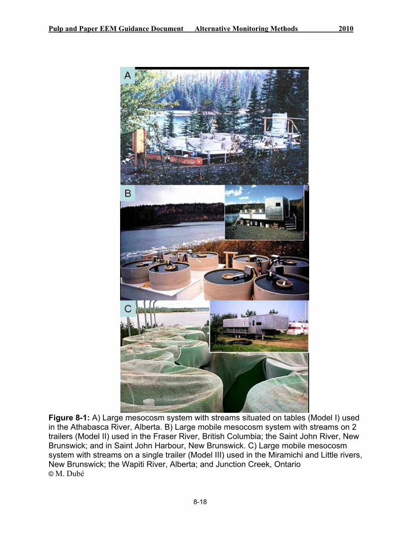
Pulp and Paper EEM Guidance Document Alternative Monitoring Methods 2010
8-18
Figure 8-1: A) Large mesocosm system with streams situated on tables (Model I) used in the Athabasca River, Alberta. B) Large mobile mesocosm system with streams on 2 trailers (Model II) used in the Fraser River, British Columbia; the Saint John River, New Brunswick; and in Saint John Harbour, New Brunswick. C) Large mobile mesocosm system with streams on a single trailer (Model III) used in the Miramichi and Little rivers, New Brunswick; the Wapiti River, Alberta; and Junction Creek, Ontario © M. Dubé

Pulp and Paper EEM Guidance Document Alternative Monitoring Methods 2010
8-19
A) B)
Figure 8-2: A) Small microcosm system with streams situated on tables over mixing reservoirs used in the Thompson River, British Columbia. B) Modular mesocosm system with streams situated on tables over mixing reservoirs used in the Little River, New Brunswick; Junction Creek, Ontario; the Wabigoon River, Ontario; and Key Lake, Saskatchewan © M. Dubé

Pulp and Paper EEM Guidance Document Alternative Monitoring Methods 2010
Head Tank
Effluent Storage
Laboratory
Streams (1 m diameter) Tables
8-20
Figure 8-3: Schematic of large mesocosm trailer system (not to scale) © M. Dubé
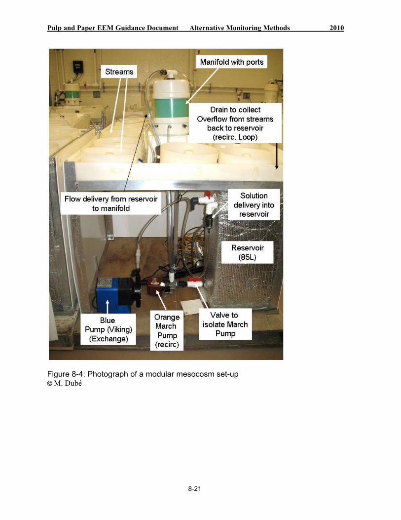
Pulp and Paper EEM Guidance Document Alternative Monitoring Methods 2010
8-21
Figure 8-4: Photograph of a modular mesocosm set-up © M. Dubé

Pulp and Paper EEM Guidance Document Alternative Monitoring Methods 2010
Distribution Manifold
8-10 L streams
Wet Table
Overflowreturn
RecircSys
ulatingtem
Total Volume = 185L (including reservoir)
8-22
Figure 8-5: Modular mesocosm flow schematic © M. Dubé
Mixing Tank
Blue Pump (1 to 4 turnovers per 24h)
85 L Reservoir
Orange Pump(Recir at ~ 30L/min)
Distribution Manifold
8-10 L streams
Overflow to drain
Wet Table
Overflowreturn
Mixing Tank
Overflow to drain
85 L Reservoir
Orange Pump(Recir at ~ 30L/min)
RecircSys
ulatingtem
Total Volume = 185L (including reservoir)

Pulp and Paper EEM Guidance Document Alternative Monitoring Methods 2010
8-23
Figure 8-6: Multitrophic Fathead Minnow reproductive bioassay and feeding barrier © M. Dubé

Pulp and Paper EEM Guidance Document Alternative Monitoring Methods 2010
8-24
Figure 8-7: Site set-up for modular mesocosms © M. Dubé

WATER
FOO
D
Ref
Effluent
NOMpHRef pH & NOM
Metal
Ref
Effluent
NOMpHRef pH & NOM
Metal
8-25
Pulp and Paper EEM Guidance Document Alternative Monitoring Methods 2010
WATER
FOO
D
A)
Reference Effluent
Ref
eren
ce Fish held in reference water
and fed chironomids raised in reference water
Fish held in effluent and fed
chironomids raised in reference water
Effl
uent Fish held in
reference water and fed
chironomids raised in effluent
Fish held in effluent and fed
chironomids raised in effluent
Multi-trophic Multi-trophic
B)
Figure 8-8: A) Factorial experimental design to investigate the importance of water vs. diet in responses of Fathead Minnow to metal mine effluent in modular mesocosms; B) Experimental design to investigate the influence of pH and natural organic matter (NOM) on Fathead Minnow responses after exposure to an MME mixture and a single metal in multitrophic modular mesocosms © M. Dubé
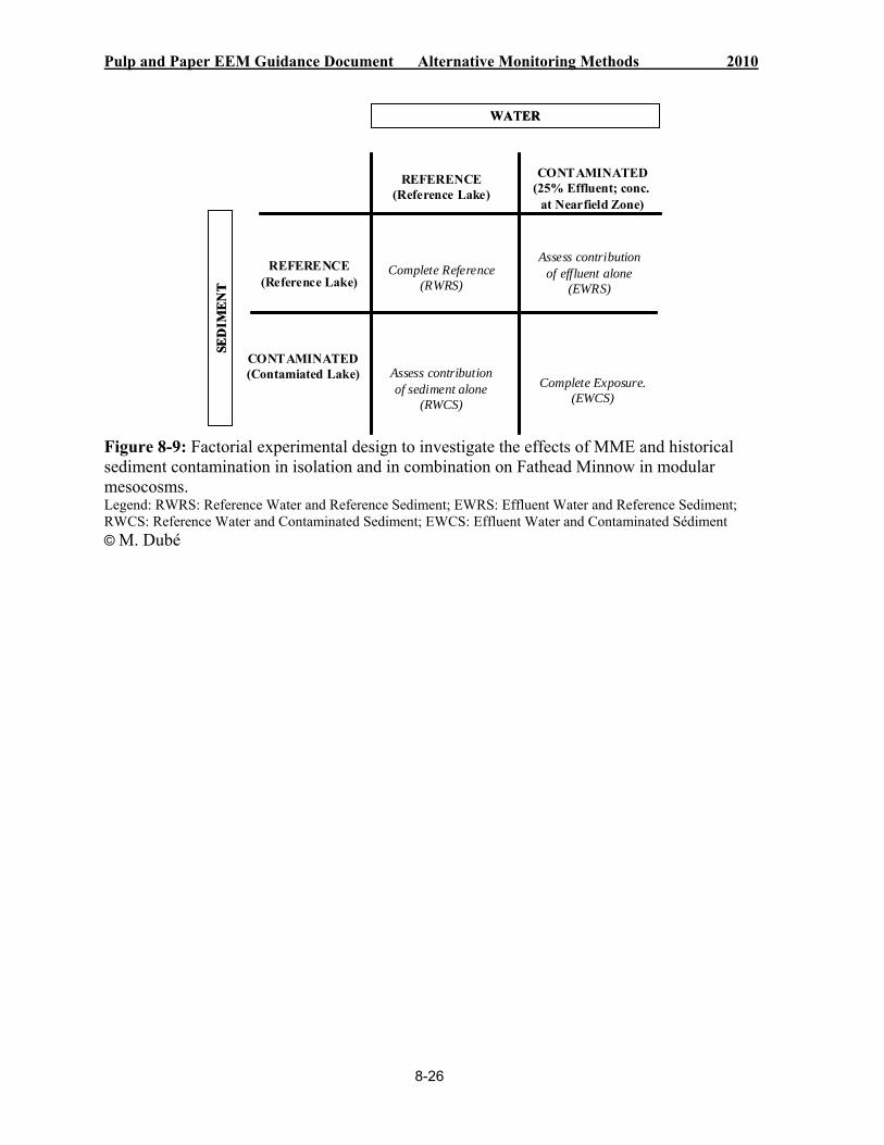
Pulp and Paper EEM Guidance Document Alternative Monitoring Methods 2010
WATER
SED
IMEN
T
WATER
SED
IMEN
T
8-26
REFERENCE(Reference Lake)
CONTAMINATED(25% Effluent; conc.
at Nearfield Zone)
REFERENCE(Reference Lake)
CONTAMINATED(Contamiated Lake)
Complete Reference(RWRS)
Assess contributionof effluent alone
(EWRS)
Assess contributionof sediment alone
(RWCS)
Complete Exposure.(EWCS)
Figure 8-9: Factorial experimental design to investigate the effects of MME and historical sediment contamination in isolation and in combination on Fathead Minnow in modular mesocosms. Legend: RWRS: Reference Water and Reference Sediment; EWRS: Effluent Water and Reference Sediment; RWCS: Reference Water and Contaminated Sediment; EWCS: Effluent Water and Contaminated Sédiment © M. Dubé

Pulp and Paper EEM Guidance Document Alternative Monitoring Methods 2010
8-27
8.2.2 Applicability within the EEM Programs
It should be emphasized that while mesocosms are a recommended monitoring alternative, their use should only be considered when field surveys cannot be designed to unequivocally answer the hypothesis, or simply cannot be conducted. Such situations include confounded receiving environments or where unsafe sampling conditions exist. Examples of confounded receiving environments include areas with the presence of historical effects, the absence of suitable reference areas for comparison to exposure areas, the presence of other effluents, and changes in relevant habitat types that cannot be factored out in the design of a field survey. Mesocosms can also be used for assessment of magnitude (dilution series) and for investigation of cause. The above-described case studies illustrate the different types of questions and experimental manipulations that can be applied to the different phases of the EEM program.
It may be possible to use the fish from a fish survey mesocosm study for the fish usability component of EEM as well, provided that the effect endpoint has the potential for responding over exposure periods typical of mesocosm studies. In this case, the effect endpoint and statistical procedures would be as outlined in chapter 3.
There are advantages and disadvantages to using mesocosms, and these should be weighed against the advantages and disadvantages of other monitoring alternatives before the final selection of an approach.
8.2.3 Mesocosm Technology
8.2.3.1 Suitability of Mesocosm Design
To maintain data quality and ensure consistent application of mesocosm technologies in EEM programs, a review of the physical design of the system used and the study design, including standard operating procedures, is required. This section outlines physical design guidance and experimental design recommendations for both a large trailer mesocosm system as well as for the smaller modular design.
Regardless of the system used, general operation is the same. Replicated tanks or streams hold the biota (fish, benthic invertebrates), algae, and/or substrate of interest. A total of 5 to 8 replicate streams per treatment is considered adequate. The systems are not static but either completely flow-through (trailer mesocosm) or partially recirculating (modular mesocosm). Ideally, reference water and dilution water are collected from a reference site and delivered to a head tank. Treated effluent is collected daily, or no less frequently than weekly, and stored on-site in a head tank. Head tank liquids can be heated or chilled depending on the circumstances. Mixing tanks are used to mix reference water and effluent to the desired test concentration. Mixed water or “treatment water” is delivered from each mixing tank to the mesocosm streams at a flow rate to achieve a target turnover time (minimum of one turnover or complete stream volume exchange every 24 hours and up to 6 turnovers per 24 hours). The experiment is typically run for 30 to 65 days, with daily and weekly measurements taken of physical and chemical variables, flows, fish mortality, and reproduction (if eggs are collected

Pulp and Paper EEM Guidance Document Alternative Monitoring Methods 2010
8-28
daily, for example). At the end of the exposure period, fish are examined and supporting measures are taken.
8.2.3.2 Description and General Operation of Large Trailer Mesocosm System
The large trailer mesocosm system, developed by the National Water Research Institute of Environment Canada, has been used to assess PME and MME effects on benthic food webs (benthic invertebrates and algae) (Culp and Podemski 1996; Culp et al. 1996, 2000a, 2001; Cash et al. 2002) and small-bodied fish (Dubé 2000; Dubé and MacLatchy 2000; Cash et al. 2002; Dubé et al. 2002). This system has been used for benthic invertebrate community assessments as well as water-borne exposures with fish. The system can still be used, although most applications now use the modular mesocosm system described in the next section.
The large trailer stream system consists of 16 circular tanks or streams, with a surface area of 0.9 m2, placed in pairs on tables that are 74 cm high (figures 8-1 and 8-3). Water from a reference area is pumped into a 378-L polyethylene head tank placed on a platform that is1.2 m high, and gravity-fed through a system of pipes to the streams. Intake pumps such as a land-based pump (e.g., commercially available irrigation or pool pumps) or a submersible pump (0.5-HP Hydro-Matic Model # SPD50-H) can be used, depending upon volume requirements, pumping distance, and the head required. Pumping reference water from a mill water intake is also a possibility. Gate valves control water flow to individual streams and allow flow rate calibration for each stream. Water is delivered to each stream at a rate of 2 L/min, resulting in a total water requirement of 32 L/min for the 16-stream system.
Water depth in the streams is maintained at 26.9 ± 0.1 cm ( ± 1 SE) by an overflow drain that returns all wastewater to the river. The overflow drains are screened to prevent fish loss and limit emigration of insects from the streams. Each stream contains 227 L of water, resulting in a hydraulic residence time of approximately 2 hours. By increasing water residence time within the streams to 4 hours, the volume of effluents and reference water required during a study is minimized. Final determination of residence time for a particular system depends upon the size of the tank used and species requirements for oxygen and temperature. If mesocosm studies are conducted in the late autumn, the head tank and water delivery lines can be wrapped with heat tape and insulated to allow the system to be operated when freezing temperatures may occur (-5°C). Shade cloth can be used to reduce solar heating in the summer.
The streams on the large mesocosm system are tanks, 107 cm in diameter, constructed of polyester fibreglass. Streams are placed on 8 tables that are 74 cm high, 2 to a table. The water outflow pipe passes through a standpipe and drains into pipes beneath. These drain pipes connect to a general outflow pipe for discharge to the river downstream of the water intake point.
For invertebrate applications, current velocity in each stream can be created using a propeller system (Podemski 1999). Water velocity in each stream near the water column midpoint is normally maintained at 20 cm/sec, although site-specific velocities should be the determining factor. Other current-generation mechanisms can be used, provided they produce the water velocities. In fish studies, current can also be generated using the propeller system, although
Pulp and Paper EEM Guidance Document Alternative Monitoring Methods 2010
8-29
spray bars attached to the water delivery system for each stream have also been used for species where water velocity is not a critical requirement.
Effluent is collected daily or every second day and stored in polyethylene containers. The point of effluent collection depends upon the study design. For the first monitoring study at a pulp mill, for example, the final effluent that is representative of what is being discharged to the aquatic environment is the target source. Effluent treatments are delivered independently and continuously to individual streams by peristaltic pumps (Masterflex ® L/S Nema-type 13 wash-down controllers and cartridge pump heads). Effluent flow rates depend upon the site-specific, environmentally relevant concentrations to be tested. For example, if plume delineation studies in the field have determined effluent concentrations to be 1%, then an effluent flow rate into each stream is set at 20 ml/min (1% of 2 L/min). If there are 16 tanks on the trailer, which are allocated between 2 treatments (8 streams for control; 8 streams for 1% exposure), then the following effluent volume is required on a daily basis: 20 ml/minute x 60 minutes/hour x 24 hour/day = ~ 29 L/day/stream x 8 streams = ~ 231 L/day. This volume would fit into a small polyethylene container.
After water and effluent flows have been calibrated for each system, the individual tanks or streams are seeded with natural substrates, algae, benthic invertebrates and/or fish species endemic to the receiving environment being studied. Inoculation of biotic populations is described below for fish and invertebrates. Further details on the construction of this trailer system can be found in the literature referenced herein.
8.2.3.3 Description and General Operation of Modular Mesocosm System
Each modular mesocosm unit or table consists of a shipping pallet, metal frame, wet table, up to 8 replicate circular polyethylene streams, a reservoir for holding the exposure solution, a manifold for equal flow distribution to the replicate streams, a blue Viking pump for flow delivery from the mixing tank to the reservoir, and an orange March pump for flow recirculation within the unit from the reservoir to the manifold/stream complex (figures 8-4 and 8-5).
Each mesocosm holds a total capacity of 185 L of water (85-L reservoir, 82.4 L = 10.3 L/stream x 8 streams, ~ 15 L in manifold/hoses/pumps) and requires 3.0 amps to run without heating, cooling or aerating the water. Each replicate circular stream has a volume of 10.3 L. There is a central non-functional standpipe in each stream. The circular high-density polyethylene streams sit on top of a table that drains into an 85-L dilution reservoir. Each stream requires a cover to keep fish in and other things (e.g., birds) out. A window screen or Nytex mesh cover is used, and secured with bungee cords. Each table has 8 polyethylene streams of 10.3 L each that are custom-made and moulded. The reservoirs are 85-L polyethylene plastic totes that are also custom-made and moulded. The 8-port manifold system was custom-designed to allow for equal flow distribution to each stream without requiring 8 separate pumps. There are 2 types/sizes of tubing in the mesocosm system to deliver water to and from the manifold and to the streams (internal diameter [ID] 3/8” and ID 3/4”).
An electronic metering pump (blue Viking/Pulsatron pump, Series E 240 GPD LEH 75A-PHC3-XXX) controls the water/effluent turnover times in the reservoir. The March “Series 3” Seal-less

Pulp and Paper EEM Guidance Document Alternative Monitoring Methods 2010
8-30
Magnetic Drive Centrifugal Pump (orange pump) controls the movement of water/effluent from the reservoir to the streams. Pumps are the most expensive part of this system and the most critical component of the study. An incorrect flow rate means incorrect dilutions to the test organisms.
Each mesocosm unit or table represents a treatment with 8 replicate streams per treatment. Note that it can and has been argued that the systems are pseudo-replicated at the level of the reservoir. This point has been successfully argued and defended through the peer-review publication process. For fish mesocosm application, streams can be fitted with feeding barriers for multitrophic studies. This mesh barrier will allow a benthic invertebrate culture to develop under treatment conditions, while controlling access for the fish above it (Figure 8-6).
Researchers have experimented with many different forms of flow delivery, including in-line mixing pumps. Based on experience, and in the interest of keeping costs manageable, mixing the treatment solutions in a mix tank and delivery using a pump to each mesocosm reservoir has become the preferred option over that of in-line mixing of water + contaminant. Water is delivered from a mixing tank to a mesocosm reservoir using a blue Viking pump at a rate of 1-4 turnovers every 24 hours (Figure 8-5). There is an overflow drain at the back of each reservoir and a baffle inside each reservoir to prevent short-circuiting of the inflow to the overflow drain.
The March pump is the recirculating pump. Flow moves from the March pump through the manifold, into the streams, overflows from each stream into the wet table, and then drains back into the reservoir through the hole in the table. The manifold must be level and free of air bubbles to operate effectively. All tubing must be the same length for the manifold to be able to pressurize equally and deliver water at an even flow rate to each of the streams. Water enters the stream along the length of water inlet tubes threaded through the stream wall. Because of the angle at which the water enters the stream, a slight circular current is created. Water fills the streams and then drains over the top, collects briefly on the tabletop, and is rerouted back down to the reservoir. Reservoirs are insulated using silver insulation sheets wrapped around the outside of the tank.
8.2.4 Considerations for Site Selection
Irrespective of the mesocosm used, there are some basic site requirements. The system is typically located at a reference area for access to reference water. In a freshwater riverine situation, reference water is pumped from upstream of the effluent outfall into the system and discharged back to the river downstream from the point of intake. This is the most straightforward scenario for mesocosm use. Distance to the reference water source is also a consideration for site selection, as extensive pumping requirements with respect to distance, or elevation (head), can exceed pump specifications for the rate required. Other site requirements include adequate space, site access, electrical power and security.
Access to power is one of the major site-selection requirements. The mill typically provides this, via a power line that the mill’s electricians install into the mesocosm’s power panel on either the trailer or the power pallet designed specifically for the modular mesocosm system. In remote areas, if power is not available, generators have been used to power the system, although this

Pulp and Paper EEM Guidance Document Alternative Monitoring Methods 2010
8-31
approach is not recommended. Due to maintenance and supervision needs, generator use is often not cost-effective.
During site set-up, the process consists of selecting the site, unloading equipment, and placing the head tanks and mixing tanks at the end opposite the power pallet (in the case of the modular system). Modular mesocosms are typically placed under a tent for shade, to reduce particulate deposition (dust), and for security purposes. The head tanks, mixing tanks and power pallet do not go under the tent (Figure 8-7). The modular mesocosm or trailer is placed in a north-south direction perpendicular to sunset/sunrise. First, all equipment is placed, then power is connected, mesocosm tables are levelled, tubing is run from head and mixing tanks to streams, all tanks are filled, pumps are turned on and calibrated, tents are set up (for modular mesocosms), and then animals are added.
It is critical to calculate the electrical requirements of the system for the experimental design selected and to assess the site to determine adequate electrical availability. Power reliability at industrial sites is an important consideration.
8.2.5 Biological Monitoring Study Designs
8.2.5.1 Overview
The objective of a study design is to outline what mesocosm and associated laboratory work is needed to complete the biological monitoring portion of the EEM study. Many of the study components are similar to those outlined in the various chapters of this document.
A study design is submitted to the Authorization Officer at least 6 months prior to the commencement of sampling for biological monitoring studies (Pulp and Paper Effluent Regulations [PPER] Schedule IV.1, subsection [ss.] 4(1)). The study design will include:
a site characterization; a description and justification for the experimental design (number of treatments,
concentrations of effluents, level of replication); the fish species, sampling areas and sample size selected; a detailed timetable for conducting the mesocosm study; a description of how the fish studies will be conducted in order to determine if there are
effects on fish populations and tissues; a description of how the benthic invertebrate community studies will be conducted in
order to determine if there are effects on the benthic invertebrate community as an indicator of effects on fish habitat;
the field and laboratory methods; and identification of the quality assurance and quality control (QA/QC) measures that will be
taken to ensure validity of the data.
Other recommended details of the study design may include:
defining the goals and expectations of the EEM study;

Pulp and Paper EEM Guidance Document Alternative Monitoring Methods 2010
8-32
determining the overall approach, including stating the rationale for choosing an alternative, which may be based on previous monitoring results;
establishing statistical design criteria: development of hypotheses, selection of statistical methods, determination of data needs (statistical significance and power analysis);
developing operating plans and procedures: sampling procedures, laboratory analysis procedures, QA/QC procedures, data storage and retrieval, data analysis; and
describing a plan for data interpretation and program evaluation.
8.2.5.2 Study Treatments
In mesocosm studies, the effect of effluent on fish is evaluated by comparing effect indicators (growth, reproduction, condition and survival) between fish held under control conditions (reference water) to those held in effluent. In mesocosm studies using benthic invertebrates, an effect is determined by comparing effect indicators (total benthic invertebrate density, taxa richness, evenness index and similarity index) between invertebrates in reference vs. exposure streams. It is crucial that mesocosm studies be designed to maximize the possibility of detecting effects if they are present. This includes selecting appropriate treatments, level of replication, sentinel species, response variables, and conducting the studies at the proper time of year.
Mesocosm studies provide for controlled experimental manipulation, with the added benefit of environmental relevance (natural water quality, photoperiod, water and air temperature). The flexibility in experimental design is one of the most significant and creative advantages of using mesocosms. Several study designs can be employed, depending upon site-specific requirements and the phase of the monitoring program (i.e., magnitude and geographic extent, and investigation of cause). In the simplest case, 2 treatments (control vs. effluent exposed) are compared. It is recommended that the environmentally relevant concentration of effluent be based upon a plume delineation study conducted during site characterization (chapter 2); thus it should represent the effluent concentration in the near-field area after complete mixing.
In some cases, additional treatments may be desired. Dose-response study designs where additional and higher effluent concentrations are used are helpful to confirm biota responsiveness and the absence of effects (see Dubé and MacLatchy 2000a; Culp et al. 2000a). Additional treatments may also be desired if more than one mill discharges into the same sampling area. Each discharge can represent an exposure treatment in the experimental design and the effects of each effluent can be examined in isolation or in combination. For example, if a mill discharges 3 effluents into the same receiver, effluent effects can be evaluated using the following treatments: control, effluent 1 (environmentally relevant concentration), effluent 2, effluent 3, effluent 1 + 2 + 3 (environmentally relevant concentration; see Table 8-1).
More recently, modular mesocosms have been used to assess water vs. dietary pathways of exposure for Fathead Minnow exposed to MME. This design was of value for investigating different metals in effluents and their causal contribution to fish response patterns. Fish were held in water (reference or effluent) and fed with the chironomid C. tentans cultured under either control water or effluent exposure conditions (Figure 8-8A). These results were compared to those of concurrent multitrophic mesocosm treatments. Studies have also been conducted to evaluate the influence of different water chemistry variables in ameliorating the toxicity of a

Pulp and Paper EEM Guidance Document Alternative Monitoring Methods 2010
8-33
metal and MME on Fathead Minnows by focusing on the effects of increased pH and natural organic matter using multitrophic mesocosms (Figure 8-8B).
8.2.5.3 Replication
In modular mesocosm systems with benthos or fish, typically 5 to 8 replicates are used. In the trailer mesocosm system employing a control/impact design with 2 treatments (reference vs. exposure), 8 replicates will be used as there are 16 tanks on the mesocosm trailer. If additional treatments are preferred, then 5 replicate streams per treatment should be the minimum number of replicates for EEM studies, as this should provide adequate power for assessing effects when streams are the level of replication and when no previous monitoring data are available. This approach is consistent with the recommended method for determining the number of sampling stations, using statistical power in field survey designs (chapters 3 and 4).
The unit of replication is less clear when the system is used to measure individual-based response variables in fish. The basis of the decision lies in the quantification of the importance of a tank or stream effect (i.e., an effect of one tank relative to another within the same treatment). In many laboratory studies where fish are held in aquaria, an assumption is made that there is no biological reason for tank differences within a treatment, and thus all individual fish measurements are pooled within a treatment (i.e., the variability attributable to tank effect is often ignored). For mesocosm studies it is suggested that a tank effect may exist, and the variation attributed to that effect requires some consideration in the statistical design. This is especially the case for longer-term exposures (e.g., 60 days). A nested analysis of variance (ANOVA) could be used in this example where the tank effect is nested within the fixed-effect factor of effluent treatment. If a tank effect exists, the level of replication should be at the stream level. If tank effects do not exist, fish can be selected as the unit of replication and pooled across streams within a treatment, resulting in significant increases in the number of replicates. For regression-based analyses (analysis of covariance [ANCOVA]), any tank differences would likely emerge as outliers in the analysis.
8.2.5.4 Sample Sizes and the Role of Effect Size
8.2.5.4.1 No Available Pre-existing (Historical) Data
Trailer Mesocosm System: In the trailer mesocosm, there is increased capacity to hold fish for longer periods than in the modular mesocosm system. For a standard fish population field survey, where there are no background monitoring data, the minimum sample size recommended is 20 sexually mature males and 20 sexually mature females of 2 fish species collected from each of the reference and exposure areas. If small-bodied fish species are chosen as one or both of the fish species, an additional 20 sexually immature fish should also be collected. The rationale for using 20 fish of each sex is that there is little change in the 95% confidence limits with increasing sample size beyond 20 fish. In trailer mesocosms, 15-20 sexually mature males and 15-20 sexually mature females of one small-bodied sentinel species are added to each tank. In addition, 20-30 juvenile fish are allocated to the same tank. These are recommended sample sizes that can be increased or decreased depending upon the species selected, the statistical power of the study design, and fish variability. If tanks within a treatment are selected as the unit of

Pulp and Paper EEM Guidance Document Alternative Monitoring Methods 2010
8-34
replication, 20 fish per sex per tank provides a mean with good precision (i.e., there is little change in the 95% confidence limits with increasing sample size beyond 20 fish). If tank effects do not exist and error terms are pooled so that fish become the unit of replication, 15-20 fish per sex per tank provides much higher replication per treatment. For example, a study design of control vs. 1% effluent with 8 streams per treatment, and 20 males, 20 females and 20 juveniles per tank, can result in 160 males, 160 females, and 160 juveniles per treatment if fish are the unit of replication.
Modular Mesocosm System: In modular mesocosm studies using benthic invertebrates or fish, sample size represents the number of streams replicated per treatment, as streams are the unit of replication. In a control-impact design, 8 streams are replicated per treatment. Each mesocosm table represents a treatment and thus this simplest design would only require 2 mesocosm tables for assessment. If additional treatments are required, a minimum of 5 replicates or samples are required for each treatment to address power requirements without pre-existing data (see below). Breeding pairs or trios can be used in each stream depending upon the objectives of the study. In the protocol developed by Ankley et al. (2001), a ratio of 2 males to 4 females (2M:4F) is used per replicate. However, this breeding ratio is too high for the mesocosm streams and certainly too many fish to sustain in a self-sustaining multitrophic mesocosm test over 21 days of exposure. Thus, the use of pair or trio (1M:2F) breeding is recommended. If breeding trios with Fathead Minnow are used in a modular mesocosm design, data from both females are assessed with a measure of central tendency keeping the level of replication at the stream level.
It is important to consider the objectives of the fish study when selecting which mesocosm system to use. While the trailer system provides for greater numbers of fish in each replicate, exposures are water-borne only and effect endpoints measured are condition, survival, organ size in adults and growth in juveniles, the latter as a substitute for size-at-age. The modular mesocosms have lower fish numbers per replicate but allow for multitrophic and/or water-borne exposures, and allow for investigations over a partial life cycle from breeding to offspring production over time in a repeat spawner such as Fathead Minnow. Reproductive variables, such as cumulative numbers of eggs produced per female per day, can be replicated over time, and distributions in egg production can be assessed for each treatment using distribution-based statistical tests such as the Kolmorogov-Smirnov test.
8.2.5.4.2 Available Pre-existing (Historical) Data
If data are available, the sample sizes to measure a certain effect size in a parameter with a targeted level of statistical power can be calculated, because sample variability is known. Larger numbers of samples are needed if parameters are highly variable, if detection of small differences between reference and exposure streams (small effect size) is desired, or if a high level of power is required. To determine the sample sizes using pre-existing data, the effect size and the statistical power level that is acceptable for the decision-making process needs to be determined. The purpose of defining an effect size and power level is to determine when the sampling program is collecting adequate information to provide decision support. Sample sizes can be calculated using methods described in Environment Canada (2002). Appendix 1 of Environment Canada (1997) provides a detailed discussion of power relationships, effect sizes and

Pulp and Paper EEM Guidance Document Alternative Monitoring Methods 2010
8-35
the benefits of reducing variability in terms of increasing power. It is recommended that and be set equally at 0.10 for power calculations.
8.2.6 Fish Monitoring – Effects Assessment
8.2.6.1 Study Design
8.2.6.1.1 Species Selection
The most important factors when selecting fish species for mesocosm studies are environmental relevance, abundance for collection, size, availability of adults and juveniles, sexual dimorphism, spawning period, and sensitivity to effluent. The recommended method for assessing effluent effects in mesocosm studies conducted in the trailer mesocosm system is by monitoring pre-spawning adults (sexually mature fish) and juveniles of one small-bodied fish species (e.g., darters, minnows, sculpins) that is relevant to the receiving environment. Monitoring of adults provides for assessment of effluent effects on survival, reproduction (energy use) and condition (energy storage). Monitoring of juveniles provides for assessment of effluent effects on survival, energy use (i.e., growth as a size-at-age substitute) and energy storage (i.e., liver size and condition).
Species selection for mesocosm studies is restricted by size requirements (numbers of fish per tank decrease with increasing fish size) and sexual dimorphism (if males and females cannot be externally sexed, increased numbers should be considered to ensure adequate sample sizes). As such, mesocosms are best suited for use with small-bodied fish species. Sampled species should also be suitable for measuring the recommended variables. To date, fish species used in mesocosm studies include Mummichog, juvenile Atlantic Salmon, Slimy Sculpin, Creek Chub, Longnose Dace and Fathead Minnow (Table 8-1).
The advantages and disadvantages of using small-bodied species in field surveys have been described by Gibbons et al. (1998a, 1998b). A small-bodied fish can be considered as a fish species that has a maximum length of 150 mm. Information on maximum growth of fish species can be found in the scientific literature, including Scott (1967), Scott and Crossman (1973), Fritz et al. (1975), Roberts (1988), Nelson and Paetz (1992), Jenkins and Burkhead (1993), Coad (1995), and Leblanc and Couillard (1995). Small-bodied fish species are usually more abundant, easier to capture, and more sedentary than larger-bodied fish species. Smaller home ranges are desirable, as it increases probability and consistency of effluent exposure compared to larger, more mobile, possibly migratory species.
There can be disadvantages to using small-bodied fish. Often, less is known about their basic biology, particularly their spawning habits, making it difficult to determine the best sample areas, times and methods. However, due to the significant amounts of data collected on small-bodied fish as part of EEM programs as well as many Canadian research studies, knowledge of small-bodied fish life-history strategies and basic biology has increased significantly (Munkittrick, University of New Brunswick, unpublished). Some species are multiple spawners (i.e., they produce more than one clutch of mature ova every year; see Heins and Rabito 1986; Burt et al. 1988; Paine 1990). This can be a disadvantage for field surveys because reproductive

Pulp and Paper EEM Guidance Document Alternative Monitoring Methods 2010
8-36
effort in these species is difficult to estimate from a single sample. Reproductive tissue can be turned over almost completely between clutches (i.e., most of the mass of ova in the ovary will be spawned and then a new clutch of mature ova will be developed). The number of clutches produced during the spawning season becomes the important reproductive variable and is difficult to estimate for an individual female in the field, even with frequent sampling. However, multiple spawners such as the Mummichog have been used successfully in mesocosm studies to evaluate effluent effects on EEM effect endpoints, including changes in gonad size (Dubé and MacLatchy 2000a; Cash et al. 2002; Dubé et al. 2002). An advantage of using controlled-exposure mesocosm studies is that the state of fractional spawners can be monitored throughout the exposure period.
The latest advances in mesocosm technology and application using the modular system has evolved around the use of Fathead Minnow in a 21- to 30-day partial-life-cycle exposure experiment (Table 8-1). Mesocosm applications using the trailer system have been successful in assessing effluent effects. However, exposures are water-borne, which lessens environmental relevance. Water-borne exposure is standard practice in fish toxicological assessments with single contaminants, but given the nature of complex mixtures, dietary pathways of exposure should be considered. For example, numerous studies have investigated the importance of the trophic-transfer of metals (Ni et al. 2000; Chen et al. 2000; Mason et al. 2000; Xu and Wang 2002) in aquatic environments. Including dietary exposure in the mesocosm approach would therefore be an improvement. The ability to directly assess reproductive output (number of eggs produced, number of spawning events and offspring survival, hatching success, deformities) after exposure to effluent, in addition to the standard EEM effect endpoints, would also be desirable for more causal investigations.
Fathead Minnows have been used extensively as a toxicological workhorse in laboratory investigations, as they represent an ecologically significant part of the Cyprinidae family, they have been extensively tested, and a large database of knowledge exists regarding their culture and life cycles (Panter et al. 2002; Ankley et al. 2001; Jensen et al. 2001). They are also used in risk assessment and government/industry monitoring studies on an international scale (US EPA 1982, 1996, 1999, 2002; OECD 2001; Shaw et al. 1995a, 1995b). In addition, Fathead Minnows are small (average length of 6 cm and width of 1 cm), fractional, substrate spawners that, under specific conditions, can easily be manipulated in captivity to produce clutches of 50-150 eggs every 3-5 days. They are also an environmentally relevant species, as they are abundant in freshwater systems across Canada. Thus, the development of a mesocosm approach using Fathead Minnows to measure EEM effect endpoints and provide focus for direct evaluation of how reproductive output is affected by effluent mixtures would be highly useful in cases where field surveys cannot be conducted. Furthermore, self-sustaining (no external food source) mesocosms wherein fish and their diet are co-cultured, resulting in fish exposure through both dietary and water-borne pathways (i.e., a multitrophic mesocosm), would also be highly relevant.
Ankley et al. (2001) developed a short-term bioassay using Fathead Minnow that assesses reproduction as well as aspects of early development in a shorter time frame than traditional life-cycle assays. The time frame of the partial-life-cycle test (21 days) made it a suitable candidate for mesocosm use. A number of investigations have used the 21-day bioassay to monitor effects of estrogenic (Harries et al. 2000; Ankley et al. 2001; Sohoni et al. 2001),

Pulp and Paper EEM Guidance Document Alternative Monitoring Methods 2010
8-37
androgenic (Ankley et al. 2003) and anti-androgenic (Jensen et al. 2004) compounds. These studies have predominantly focused on single contaminants that do not represent the complexity of effluents. A limited number of investigations into the effects of industrial effluents using the 21-day bioassay have been conducted (Martel et al. 2003; Parrott 2005). However, these studies have used differences in methodology (e.g., number of independent replicates, number and type of variables measured) and were conducted in the laboratory under water-borne exposure conditions.
Development of the Fathead Minnow 21-day bioassay for use in EEM mesocosm studies first required in situ use with natural receiving water, yet controlled temperatures and photoperiods (Rickwood et al. 2006a, 2006b). As the chironomid C. tentans life-cycle bioassay had been previously established for use in the modular mesocosm system (Hruska and Dubé 2004, 2005), the next step was to combine these tests into a multitrophic mesocosm test for use in the modular mesocosm system. This was first done in the lab with controlled water temperature (Rickwood et al. 2006c) and then moved to the field, with full testing under ambient temperatures and photoperiods and using ambient reference water (Pollock et al. 2009; Rickwood et al. 2008). The Fathead Minnows used in these studies have been laboratory cultured and transported to the site to control for fish quality, age, state of reproductive development and exposure (or lack thereof).
8.2.6.1.2 Effect Indicators
Trailer Mesocosm System: The effect indicators measured in the trailer mesocosm study using fish are the same as those measured in a field survey. Effects on fish growth, reproduction, condition and survival are determined in answer to the question, “Has the fish population been modified by effluent?” Survival, growth and reproduction (energy use), and condition (energy storage) are measured to detect any effluent-related effect on the fish population. All of these measurements can be taken from fish exposed to effluents in mesocosm studies (Table 8-2).
Growth is the change in size (weight or length) with time or age. Mesocosm studies over a longer exposure period (45-60 days) can assess effluent effects on juvenile growth, specifically changes in total body weight and length relative to control fish. In mesocosms, growth is measured in YOY (young of the year) or juvenile fish from the start of the study to the end, a duration of 6-8 weeks depending upon the temperature during the study. The determination of growth effects over a short exposure period requires that studies be conducted during warm water temperatures and with a sentinel species that has a high growth rate. Kneib and Stiven (1978) have shown that juvenile growth rates of Mummichog, for example, are very high post-hatching (an increase of 15 mm in 2 months), which makes them ideal candidates for assessing the effects of effluent on growth. Other studies using YOY Slimy Sculpin have shown that growth effects can be measured after only 26 days of effluent exposure (Dubé et al. 2005). Although length and weight measurements are taken in adults, growth is unlikely during the short duration of the mesocosm studies.
Table 8-2: Fish mesocosm study effect indicators and endpoints and related statistical procedures
Effect Indicators
Effect and Supporting Endpoints Statistical Procedure
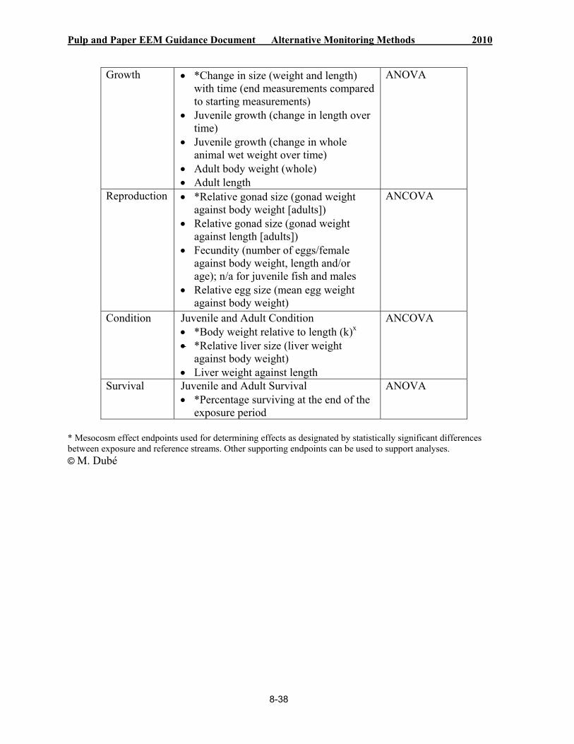
Pulp and Paper EEM Guidance Document Alternative Monitoring Methods 2010
8-38
Growth *Change in size (weight and length) with time (end measurements compared to starting measurements)
Juvenile growth (change in length over time)
Juvenile growth (change in whole animal wet weight over time)
Adult body weight (whole) Adult length
ANOVA
Reproduction *Relative gonad size (gonad weight against body weight [adults])
Relative gonad size (gonad weight against length [adults])
Fecundity (number of eggs/female against body weight, length and/or age); n/a for juvenile fish and males
Relative egg size (mean egg weight against body weight)
ANCOVA
Condition Juvenile and Adult Condition *Body weight relative to length (k)x *Relative liver size (liver weight
against body weight) Liver weight against length
ANCOVA
Survival Juvenile and Adult Survival *Percentage surviving at the end of the
exposure period
ANOVA
* Mesocosm effect endpoints used for determining effects as designated by statistically significant differences between exposure and reference streams. Other supporting endpoints can be used to support analyses. © M. Dubé

Pulp and Paper EEM Guidance Document Alternative Monitoring Methods 2010
8-39
Table 8-3: Recommended (shaded) response variables and suitable additional supporting information, and suggested statistical analysis for Fathead Minnow application in modular mesocosm systems
Type of Response
Response Variable
Dependent Variable (Y)
Independent Variable (X)
Covariate (X)
sStatistic (Single Factor)
Statistics (Two
Factors) Stage of experiment: Pre-exposure (for fish that met criteria)
Energy Use (Adults)
Mean total egg ctionprodu
(number)
Mean total number of eggs per breeding group
Treatment n/a ANOVA
) (one-wayANOVA (two-way)
Mean egg production (number)
n number Meaf eggs o per
female per day Treat t men n/a
ANOVA (one-way)
ANOVA (two-way)
Cumulative er eggs p
le pefema r day ber) (num
ulative Cums per eggale fem
Day n/aKolmogorov-Smirnov
Kolmogorov-Smirnov
Mean total spawning events (number)
Mean total number of spawning events per breeding group
tTreatmen n/a Chi-Square Chi-Square
Offspring
Fertilization s (%succes )
Number of eggs fertilized/ number of eggs laid x 100
Treatment n/a ANOVA
) (one-wayANOVA (two-way)
Stage of experiment: Exposure
Adult Survival
Mean adult survival (%)
Number of adults surviving at end/Number of adults at start x 100
Treatment n/a ANOVA (one-way)
ANOVA (two-way)
Energy Storage (Adults)
Condition (g/cm)
Total body weight (log)
n/a Length (log) ANCOVAANCOVA (two-way)
Relative liver size (g)
Liver weight (log)
n/a Total body w ) eight (log
ANCOVA ANCOVA (two-way)
Liver weight (log)
n/a Length (log) ANCOVAANCOVA (two-way)
Relative egg size (µm)
Mean egg size (log)
n/a Total body weight (log)
ANCOVA ANCOVA (two-way)
Mean egg size (log)
n/a Length (log) ANCOVA ANCOVA (two-way)
Energy Storage (Adults) (If ANCOVAs
Mean condition factor (%)
Total body weight/ (length)^3 * 100
Treatment n/a ANOVA (one-way)
ANOVA (two-way)

Pulp and Paper EEM Guidance Document Alternative Monitoring Methods 2010
8-40
cannot be done due to lack of spread on x axis)
LSI (%) Liver weight/body weight * 100
Treatment n/aANOVA (one-way)
ANOVA (two-way)
GSI (%) Gonad weight/body weight * 100
Treatment n/aANOVA (one-way)
ANOVA (two-way)
Energy Use (Adults)
Total body weight (g)
n/a Treatment n/aANOVA (one-way)
ANOVA (two-way)
Fork length (cm)
n/a Treatment n/aANOVA (one-way)
ANOVA (two-way)
Relative gonad size (g)
Gonad weight (log)
n/a Total body weight (log)
ANCOVA ANCOVA (two-way)
Gonad weight (log)
n/a Length (log) ANCOVAANCOVA (two-way)
Cumulative eggs/breeding group/day (number)
Cumulative eggs/breeding group
Day n/aKolmogorov-Smirnov
Kolmogorov-Smirnov
Mean total egg production/ day (number)
Mean total number of eggs/female/ day
Treatment n/aANOVA (one-way)
ANOVA (two-way)
Mean egg production/ day (number)
Mean number of eggs/ female/day
Treatment n/aANOVA (one-way)
ANOVA (two-way)
Cumulative spawning events/ breeding group/day (number)
Cumulative total number of spawning events/ breeding group
Day n/aKolmogorov-Smirnov
Kolmogorov-Smirnov
Mean total spawning events/day (number)
Mean total number of spawning events/female/day
Treatment n/a Chi-Square Chi-Square
Relative fecundity (number)
Number of eggs/female (log)
n/a Total body weight (log)
ANCOVA ANCOVA
Number of eggs/female (log)
n/a Length (log) ANCOVA ANCOVA
Other Adult Reproductive Responses
Development of secondary sexual characteristics
Presence/ absence of tubercles; banding; fin dot; fat pad
Treatment n/a Chi-Square Chi-Square
Rank of ovipositor size
Treatment n/a Chi-Square Chi-Square
Reproductive hormones
Male/female testosterone (ng/g)
Treatment n/aANOVA (one-way)
ANOVA (two-way)
Female estrogen (ng/g)
Treatment n/aANOVA (one-way)
ANOVA (two-way)

Pulp and Paper EEM Guidance Document Alternative Monitoring Methods 2010
8-41
Male vitellogenin (ng/g)
Treatment n/aANOVA (one-way)
ANOVA (two-way)
Gonadal histology
Number and stage of cells
Treatment n/a Chi-Square Chi-Square
Offspring
Mean hatching success (%)
Number of eggs hatched/ number of eggs fertilized x 100
Treatment n/aANOVA (one-way)
ANOVA (two-way)
Mean total deformities (%)
Total number of deformities at hatch/total number of larvae x 100
Treatment n/aANOVA (one-way)
ANOVA (two-way)
Mean fertilization success (%)
Number of eggs fertilized/ number of eggs laid x 100
Treatment n/aANOVA (one-way)
ANOVA (two-way)
Mean larval survival (%)
Number of larvae survived after 5 days/total number of larvae x 100
Treatment n/aANOVA (one-way)
ANOVA (two-way)
Mean days to hatch
Mean number of days to hatch
Treatment n/aANOVA (one-way)
ANOVA (two-way)
Water Chemistry
In situ measurements
Various Treatment n/aANOVA (one-way)
ANOVA (two-way)
Lab analysis Various Treatment n/a ANOVA (one-way)
ANOVA (two-way)
Fish Tissue Body Burden
Lab analysis Various Treatment n/a ANOVA (one-way)
ANOVA (two-way)
Fish Tissue - Gonads Lab analysis Various Treatment n/a
ANOVA (one-way)
ANOVA (two-way)
Fish Tissue - Gills
Lab analysis Various Treatment n/a ANOVA (one-way)
ANOVA (two-way)
Fish Tissue - Liver
Lab analysis Various Treatment n/a ANOVA (one-way)
ANOVA (two-way)
Chironomid Tissue
Lab analysis Various Treatment n/a ANOVA (one-way)
ANOVA (two-way)
Algal Tissue Lab analysis Various Treatment n/a ANOVA (one-way)
ANOVA (two-way)
Sediment Analysis
Lab Analysis Various Treatment n/a ANOVA (one-way)
ANOVA (two-way)
Legend: LSI: Liver Somatic Index; GSI: Gonadosomatic Index. © M. Dubé
Reproduction is expressed as reproductive effort, fecundity, egg size or gonad weight relative to body size. To date, mesocosm studies have examined changes in gonad size to assess effluent

Pulp and Paper EEM Guidance Document Alternative Monitoring Methods 2010
8-42
effects on reproductive function. However, measures of fecundity and egg size are easy to measure, if an appropriate sampling time is chosen. Ideally, exposure studies should commence 6-8 weeks prior to the spawning season in order to assess effluent effects on gonad weight.
During the mesocosm study, the physical state of the fish is also assessed. A visual estimation of physical malformations and lesions on the body surface, including eroded, frayed or hemorrhagic fins, parasites, or other physical deformations, is required.
Modular Mesocosm System: The response variables measured in the modular system, which has been used primarily with Fathead Minnow, are summarized along with suggested statistical analysis procedures in Table 8-3. The variables shaded in grey are those recommended for use. Those variables that are not highlighted are variables that have been measured in different study designs and could be included to provide additional support. It is important to note that use of the standardized Ankley et al. (2001) 21-day reproductive assay has been modified for improved application under the EEM program and specifically for use in mesocosms as an alternative to the fish survey. The methods are described below and remain to be validated and standardized by the EEM Science Committee. Mills proposing this alternative approach should expect to evaluate the response variables to be measured and should include additional supporting variables to adapt and improve this method for use in their EEM program.
8.2.6.1.3 Timing and Duration of Effluent Exposure
The timing of the mesocosm study is important and is dependent upon the test species. Water temperatures affect the experimental design. If a study is being conducted in the spring when the water is cold, exposure times may be longer, especially if a response such as growth is being measured. Temperatures below -5°C are prohibitive to mesocosm operation due to freezing of water lines.
Mesocosm studies should strive to balance duration with cost-efficiency. Exposures of 21-45 days are common for invertebrate community studies in either mesocosm system. Exposures of 21 days are common if the Fathead Minnow partial life cycle is being used as the sentinel species in the modular mesocosm system. If the trailer system is being used for a water-borne exposure, 30 days is common during summer and fall months, and has been used to measure changes in adult organ size (liver size, gonad size) and growth rates of YOY Slimy Sculpin as a result of effluent exposure.
All mesocosm studies should be conducted during normal industrial operations. Effluents should be representative of normal operating conditions. For example, storing of pulp mill effluents during shifts from hardwood to softwood furnish or during periods of bleach-plant shutdowns should be avoided. Studies should be conducted when the mill is using a consistent furnish. Mesocosm studies should not be conducted when effluent has not been discharged for long periods or during wastewater treatment upsets. Ensure any planned shutdowns are identified well in advance and studies are not affected.
Trailer Mesocosm System: Timing of the mesocosm study is important and dependent upon the spawning cycle of the fish species. See Chapter 3 for additional information on spawning cycles

Pulp and Paper EEM Guidance Document Alternative Monitoring Methods 2010
8-43
and seasonal sampling. Ideally, for spring spawners, studies will be conducted 6-8 weeks before spawning commences. For early spring spawners where it is impossible to study for this length of time prior to the spawning season, studies should be conducted as late in the year as possible to allow for gonadal senescence and recrudescence. For fall spawners, a spring or summer survey is appropriate. However, this may not apply to fish in which ova mature rapidly. For example, some late-spring-spawning minnows should be studied in early spring, rather than in fall, when ova may still be immature. Water temperatures are also a consideration for timing of studies where juvenile growth rates are higher during the summer months.
Modular Mesocosm System: The modular system, when used with Fathead Minnow, is on-site for a 10-14 day pre-exposure (length depends upon when fish meet appropriate baseline selection criteria) and a 21- to 30-day exposure period. Studies should be conducted from May to late September when water and air temperatures are between 15°C and 28°C.
8.2.6.2 Fish Methods
8.2.6.2.1 General Set-up – Trailer Mesocosm System
Once the trailer mesocosm system has been transported to the study site and reference water and power have been connected, substrate can be added to the streams and water flow rates can be calibrated. Depending upon the site-specific substrate characteristics, washed and crushed gravel, or sand, can be placed into each tank to a depth of 5 cm. In previous studies, large washed rocks were also added to each tank to serve as refuge for the fish.
Fish are collected from a reference area that is not exposed to the effluent being studied. Obviously, collection requires non-lethal sampling techniques including minnow traps, trap nets or electro-fishing with barrier nets (Portt et al. 2006). Fish are usually sorted in the field to ensure adequate numbers of juveniles and of adults of each sex (if sexually dimorphic), and to collect fish of similar size-classes. If the species chosen is not sexually dimorphic, an assumption is made that sex ratios in the field are equal and the fish should be randomly allocated to the tanks. Fish are transported back to the study site in containers with covers and under adequate aeration. If reference areas are not available, hatchery-reared fish can also be used if these fish are relevant to the study area.
At the study site, and preferably within the same day, fish are measured for length and weight, and randomly assigned to each stream. The precision of these measurements is as described in Chapter 3, with increased precision when using small-bodied species. The optimal numbers of fish per stream are 20 adults of each sex and 20-30 juveniles. To ensure random allocation of fish to streams, 16 aerated buckets with reference water are set up. Fish are measured and placed, one by one, until each bucket contains 1 fish. This procedure is repeated until all buckets have 5 fish each. Buckets are then randomly allocated to the streams and the procedure is repeated until target sample sizes are attained in the streams. It is essential that this procedure be followed to ensure that the largest fish, for example, are not all allocated to the first few streams.
There are 2 possible fish allocation scenarios. Both adults and juveniles can be allocated to the same tanks if juvenile growth rates will be based solely on starting and ending length and weight

Pulp and Paper EEM Guidance Document Alternative Monitoring Methods 2010
8-44
measurements, and adults are not cannibalistic. If juveniles will be sampled during the course of the study for growth (perhaps juveniles are tagged and repeated measurements are conducted), allocating adults and juveniles to different tanks (or different areas within a tank if these areas can be physically separated) would be recommended to minimize adult capture stress. Mesocosm streams are randomly assigned to each study treatment (control, effluent) and fish are randomly allocated to each stream. This ensures a randomized distribution to minimize stream differences due to factors such as stream position on the trailer.
After inoculation, fish are acclimated to artificial stream conditions for a minimum of 72 hours prior to effluent addition or until fish are feeding. Streams should be covered with netting to minimize fish loss due to escape or predation by birds. During the exposure period, which extends from 30 to 60 days, fish should be fed trout pellets at a rate of 4-6% total body weight per tank per day. The size of the pellets is dependent upon the size of the species used. In previous studies, trout pellets were crushed prior to feeding.
8.2.6.2.2 General Set-up – Modular Mesocosm System
In the modular mesocosm system, each system consists of a table (one per treatment) holding 5-8 replicate (preferred), 10.3-L, circular, high-density polyethylene streams. The replicate streams sit on the table, which drains into an 85-L dilution reservoir as previously described. If the trophic-transfer system is being used, each stream consists of a sediment (pre-cleaned silica sand) culture of the chironomid C. tentans, a feeding barrier, spawning tile and one breeding group of Fathead Minnow (Figure 8-6) (Rickwood et al. 2006c, 2008). The feeding barriers are used to control Fathead Minnow access to the C. tentans that have established in the substrate during the pre-exposure portion of the study. Each circular barrier contains a 1/8” (0.32 cm) square mesh screen with a pie-shaped opening of 1/10th of the stream area (approximately 71 cm2) that is turned every second day to dispense the appropriate amount of food (1 g C. tentans/day) (see below on culturing appropriate densities of C. tentans).
Pre-exposure Design: Six-month-old, naive Fathead Minnow are obtained from a reputable culture laboratory. Fish are typically transported to site by ground or air within 24 hours in oxygenated bags with water inside coolers. Upon arrival, containers are aerated and allowed sufficient time for acclimation to ambient temperatures. Reference water is slowly added to acclimate. Once acclimatized, fish should be placed into an appropriate holding tank to become reproductively stimulated prior to the pre-exposure breeding trial. This stimulation period should last for approximately 3 days.
The Fathead Minnow modular mesocosm method requires a pre-exposure and exposure trial. The pre-breeding trial normally consists of double the number of required breeding groups, which are bred in independent replicates in the absence of effluent to establish baseline reproductive performance. At the beginning of the breeding trial, total body weight (g), fork length (mm) and secondary sex characteristics are recorded. Secondary sex characteristics include banding, nuptial tubercles, dorsal pad and fin dot in males and ovipositor size in females (Parrot and Wood 2001). Female Fathead Minnow are size-matched, if possible, to within 25% of the male body length (Pollock et al. 2008). Each breeding pair is fed 0.5 g of frozen bloodworms twice daily throughout the pre-exposure period. Each day prior to feeding and recording of water quality, breeding tiles in each stream are checked for egg deposition. If

Pulp and Paper EEM Guidance Document Alternative Monitoring Methods 2010
8-45
breeding has occurred, eggs will be gently rolled off of the spawning tile into petri dishes with reference water and photographed for digital counting. At the end of the breeding trial, breeding groups will be selected for the exposure phase of the experiment. Breeding groups (pairs or trios, depending upon the study) are selected on the basis that there is 100% survival of all adults, that eggs are present in each replicate at least once in the immediately preceding 7 days, and that > 80% fertilization of eggs has occurred (OECD 2006; US EPA 2007). Breeding groups at both extremes (superior breeders and breeders with very few eggs) should be excluded from the study. The selected groups should be distributed throughout the mesocosm treatments and streams so as to minimize variance between the treatments. Statistical analyses are performed prior to final selection to ensure that there are no significant differences among and between treatments before effluent exposure commences. The unit of replication is n = 5-8 per treatment.
Trophic-transfer system: The trophic-transfer system and associated sediment cultures of the chironomid C. tentans are set up during the pre-exposure period. Target invertebrate densities in each stream are based on an optimal daily feeding amount of 1 g/breeding pair/day (Rickwood et al. 2006a, 2006b). Seven-day-old C. tentans larvae are shipped to the site once per week for 3 weeks to establish the cultures in the mesocosm streams before adding the fish. The larvae are obtained from a reputable culture supplier. C. tentans will have been exposed to the effluents for at least 7 days prior to the introduction of the fish, to ensure dietary exposure. In addition, this ensures that C. tentans will be at various life stages (egg, larvae, pupae, adult) within the streams to maintain a healthy breeding cycle. The number of invertebrates required to sustain the fish over 21 days in each stream is calculated based on the average number of C. tentans that emerge from one egg sac (~ 300) and by determining the number of third and fourth instars with a combined weight of 1 g (~ 50 3rd and 4th instars). Once it is known how many C. tentans weigh 1 g, the total number of C. tentans needed for the entire 21-day exposure period will be calculated (50 C. tentans/g x 21 days = 1050 C. tentans or 350 7-day-old larvae/stream/week for 3 weeks).
Once the larvae have arrived at the site, they are acclimated using treatment water in their individual containers, by adding 25% of the treatment water to each container 4 times in 12 hours. The larvae are acclimated to the ambient temperature by slowly lowering the water temperature in a water bath no faster than 1°C every 1-2 hours. Once the C. tentans are acclimated to the ambient temperature and effluent water, they are distributed among the artificial streams and fed Tetramin slurry (100 g Tetramin flakes to 1000 ml reference water) at a rate of 10 ml in the first week, 20 ml in the second, and 30 ml in the third and subsequent weeks, 3 times/week. It is recommended that 3 sediment cores (core sampler area approximately 9 cm2) be taken from each stream at the end of the pre-exposure period before fish placement so that invertebrate densities can be calculated.
Exposure Design: Once Fathead Minnow are allocated to the treatment streams, treatment solutions are delivered to the mesocosms as previously described, and the exposure period commences.
8.2.6.2.3 Maintenance and Monitoring

Pulp and Paper EEM Guidance Document Alternative Monitoring Methods 2010
8-46
Daily maintenance for the duration of the study includes calibration of flows to each reservoir to ensure target effluent dilutions are attained, cleaning of screens, and feeding of fish. Screens are placed over the water outlet pipes on each stream to prevent fish loss. These screens may require daily cleaning.
Daily monitoring requirements for each stream include recording of any fish mortality and monitoring of physical water variables, including temperature, dissolved oxygen, conductivity and pH. These measurements can be taken using YSI Inc. instruments or continuous recording equipment such as hydrolabs or thermisters. Dissolved oxygen is of critical importance, especially in studies using effluents high in organic content (e.g., pulp mill effluents). Dissolved oxygen levels should be maintained above 60% (minimum), and preferably above 80%, in all streams, using aeration if required.
For the modular mesocosm system, daily observations and measurements can include egg production, hatching success and larval survival (Table 8-3). Breeding tiles are checked daily at the same time and before feeding or water quality measurements are taken. Eggs are removed from the tiles and photographed. A consistent sub-sample of eggs from each productive brood can be collected for future analysis and total egg production corrected for this removal. Remaining eggs are then rolled into an egg cup and placed in the appropriate aerated culture tubs with treatment water. Twenty-four hours after spawning, the eggs are photographed again to check fertilization success. They are then left undisturbed until all eggs are either hatched or dead (~ 4-5 days). Once larvae have hatched, they are preserved in 10% formalin for latter enumeration and examination for deformities where the latter is a desired parameter for supporting assessments.
8.2.6.2.4 Sampling and Analysis of Fish
At the end of the exposure period, fish are anaesthetized and fork length (mm), whole body weight (g) and secondary sexual characteristics are recorded. Fish are then euthanized by spinal severance, and gonads, liver and eviscerated (carcass) weights are recorded. All streams should be sampled on the same day and all fish from each stream should be sampled before progressing to the next stream.
The measurements required and level of precision are the same as those outlined in Chapter 3. Sample preparation, laboratory analysis and QA/QC procedures for mesocosm studies are the same as those required for field fish surveys.
8.2.6.3 Data Assessment and Interpretation
8.2.6.3.1 General Requirements
Similar to field studies, in mesocosm studies, data assessment and interpretation follow each monitoring or assessment phase. In data assessment and interpretation, the following questions are answered:
Is there an effect? Is the effect mill-related?

Pulp and Paper EEM Guidance Document Alternative Monitoring Methods 2010
8-47
Is the magnitude and extent of the effect known? Is the mill-related cause of the effect known?
An overview of data analysis and interpretation for mesocosm studies is presented here.
8.2.6.3.2 Statistical Analysis of Parameters
To determine whether there is an effect on fish exposed to effluents in mesocosm streams, statistical analyses of the data are conducted of the biological variables, as suggested in Table 8-2 for the trailer mesocosm system and Table 8-3 for the modular mesocosm system with Fathead Minnow. Table 8-3 lists typical analytical approaches for two types of experimental designs: single-factor ANOVA (e.g., effect of effluent) or two-factor ANOVA (e.g., effect of effluent and contaminated sediment).
Sex differences in growth rate, body weight, condition factor, gonad size and liver size are common due to differences in overall energetic requirements between male and female fish. Therefore, for all parameters, sexes should be treated separately when estimating variability. Immature or juvenile fish should also be treated separately. The analyses that are suggested in tables 8-2 and 8-3 are preferred. However, other analyses for specific parameters can be conducted depending upon the variability of the data set. For example, in mesocosm studies, individuals of a similar size-class are selected for placement in the streams, resulting in reduced variability in parameters compared to those measured in field surveys. Thus the range over which regressions such as ANCOVAs are conducted for mesocosm data is narrow enough that ANOVAs on original organ weights (liver size, gonad size) and ratio metrics (LSI, GSI) or condition factors are justified in this instance.
Statistical considerations specific to mesocosm data sets are stated below. Additional reference can be found in the literature cited in Table 8-1.
8.2.6.3.3 Nested ANOVA Analyses
For any variable measured once on a whole replicate stream, the statistical design is a simple t-test, comparing exposed and control treatments (control/impact design). The mesocosms or streams are replicates for the treatments. However, all biological and biochemical variables are measured on replicates at a lower level—either individual fish or composites of several fish within streams. A nested ANOVA can be used to analyze these variables. If the variance among replicate streams within a treatment (Error I) is large relative to the variance among fish or composite samples within streams (Error II), then the nested ANOVA is effectively a t-test comparing treatments, with the stream means as replicate observations. However, if Error I is not large relative to Error II (e.g., p > 0.25), then the two error terms can be pooled to increase the power of the test comparing treatments (i.e., individual fish or composite samples rather than streams are used as replicates).
8.2.6.3.4 ANCOVA Analyses

Pulp and Paper EEM Guidance Document Alternative Monitoring Methods 2010
8-48
Most parameters are normally estimated using ANCOVA, as discussed in Chapter 7. This is often unnecessary in mesocosm studies, as mentioned above, unless limited fish availability prevented the standardization of size and age.
8.2.6.3.5 Data QA/QC and Analysis
The importance of ensuring data quality cannot be overstated. There are basic requirements for study design, consistency of methods and measurements, and definition of protocols and procedures; these are outlined in detail in Chapter 7.
8.2.7 Benthic Invertebrate Community Monitoring - Effects Assessment
8.2.7.1 Study Design
8.2.7.1.1 Species Selection
The benthic community that is established in the mesocosm streams is representative of that found in the reference field areas. Benthic samples are collected from the river and the entire community is inoculated into each mesocosm stream. Culp et al. (1996, 2001), Podemski (1999) and Culp et al. (2000a) have conducted studies that compared the community structure of benthic invertebrates in the mesocosm streams to that of field communities at reference areas. No ecologically significant differences in structure were observed, illustrating the effectiveness of the inoculation procedures and the suitability of mesocosms for testing effluent effects on environmentally relevant communities of benthic invertebrates.
8.2.7.1.2 Effect Endpoints
All the effect endpoints (total benthic invertebrate density, taxon richness, Simpson’s Evenness Index, similarity index [Bray-Curtis]) used to assess effluent effects on benthic invertebrates in EEM field surveys can be measured in mesocosm studies. Diversity, taxon density, proportion or presence/absence are recommended to allow for the interpretation of effects (chapter 4). These effect endpoints are summary metrics selected to encompass the range of responses that may result from effluent, including changes in productivity, species composition and biodiversity. Many other benthic invertebrate descriptive metrics are available in the literature (for a review see Resh and McElravy 1993) and may be used, if applicable, on a site-specific basis to aid in the interpretation of effects determined with the effect endpoints listed above.
8.2.7.1.3 Timing and Duration of Effluent Exposure
Mesocosm studies using benthic invertebrates can be conducted at any time from early spring to late fall. The primary limiting factor is temperature, with air temperatures below -5°C prohibitive to mesocosm operation due to freezing of water lines. Studies should be conducted during periods when field communities are under maximal effluent exposure for improved environmental realism. Studies should also be conducted at the time of year when the benthic invertebrate diversity is highest and water temperatures are conducive to growth. If historical data exist, it would be useful to examine the data and, if appropriate, conduct the study during

Pulp and Paper EEM Guidance Document Alternative Monitoring Methods 2010
8-49
similar periods so that the studies can be compared. Subsequent monitoring should also be conducted during similar periods of the year to be comparable.
The duration of the mesocosm studies for benthic invertebrate programs is typically 30-45 days, including a 7- to 12–day inoculation period for primary producers and a 25- to 30-day effluent exposure period. Effluents are collected daily or every second day during the studies and should be representative of normal industrial operating conditions.
8.2.7.2 Benthic Invertebrate Methods
8.2.7.2.1 Mesocosm Trailer – General Set-up
General set-up requirements specified in sections 8.2.3.2 and 8.2.3.3 also apply to benthic invertebrate studies. The recommended total flow of reference water or of dilution water and effluent into each stream is 2 L/minute. This flow rate results in a 2-hour volume turnover time for each stream (stream volume 227 L). Stream volume turnover rates of 4 hours have been used to reduce effluent requirements. However, longer turnover rates are not recommended due to the effects on stream temperature and dissolved oxygen. For invertebrate applications, current velocity in each stream can be created by a belt-driven propeller system. Current in each stream is established based on site-specific conditions but is normally set between 10 and 20 cm/second.
Prior to placement of substrate into the streams, five sampling bags (0.1 m2, 500-m mesh) are installed on the stream bottom. These bags are lifted at the end of the experiment, resulting in 5 sub-samples per stream. A standardized benthic environment is created in each stream to simulate the dominant environmentally relevant habitat type. To date, mesocosm studies using benthic invertebrates have focused on riverine habitats where riffle substrate is dominant. The bottom of each stream and the sampling bags are covered with an 8-cm layer of washed gravel (stones of 1-2 cm in diameter). The gravel is then left to colonize for a 7- to 12–day period to allow sufficient algal and microbial growth. Only water delivery to the mesocosm streams occurs (2 L/minute) during this colonization period. The duration of the colonization period is site-specific and depends upon temperature and colonization of algae from the river into the system.
Following the algal colonization period, existing benthic communities are transplanted to the stream mesocosms. The transplantation protocol is determined on a site-specific basis. The following is an example of inoculation protocol for a riverine, riffle habitat with a large cobble/gravel-dominated substratum (Podemski 1996; Podemski and Culp 1996; Culp and Cash 1995; Culp et al. 1996) (Table 8-1):
1. Large cobbles (surface area ~ 535 cm2) are randomly selected from the river at the reference area for placement into the mesocosm streams with their associated periphyton and invertebrate biota. These cobbles provide additional substrate and also stock the streams with a natural community of periphyton and benthic invertebrates.
2. During collection, the stones are enclosed with a 0.1-m2 U-net (500-m mesh) (Scrimgeour et al. 1993), carefully lifted from the stream bed, and placed into a container with river water. In addition, the gravel substratum beneath the stones is gently disturbed (to a depth of 5 cm)

Pulp and Paper EEM Guidance Document Alternative Monitoring Methods 2010
8-50
to collect any invertebrates under and around the base of the stone. The container is carefully transported to the mesocosm so as not to dislodge the periphyton and invertebrates associated with the stone. The cobbles are randomly placed in the artificial streams, oriented to the water flow in a manner similar to their original orientation in the natural environment. This process continues until the appropriate density (e.g., 10 large cobbles/artificial stream) of large cobbles is reached, based on natural substratum composition. Other samplers may be used to inoculate the streams with benthic communities, as outlined in Chapter 5. The objective, however, is to establish ambient densities in the mesocosm streams. To determine the number of river samples to place in the streams, the mesocosm stream area (0.9 m2) is divided by the area of the selected sampler. This random allocation of sub-samples from pooled invertebrate-community samples ensures that the initial invertebrate composition is similar among streams and limits the amount of variability in community composition among mesocosms that can be attributed to the pattern of species introduction (Wrona et al. 1982).
3. An additional series of benthic samples (biota only) are collected from the reference area and are pooled into a common container to estimate initial composition and density. Sub-samples are then removed and randomly inoculated into each artificial stream until the density of invertebrates approximates ambient densities.
Standardization of inoculation protocols is important because the sequence through which species from a common-source pool are added to mesocosms can produce large differences in community structure; these dissimilarities are unrelated to the intended study treatments (Drake et al. 1996). The test community includes multiple trophic levels constructed from random samples taken from the study river. Consequently, measurements of community-level variables, such as species composition, community production/respiration, and decomposition, are possible. These community-level variables integrate both the direct effects of stressors and, importantly, indirect ecological effects that cannot be simulated in single-species or simple food-chain systems (e.g., competition-mediated shifts in community structure, or biomagnification) (Carlisle 2000).
Following biotic inoculation, the mesocosm system is left to acclimatize for 24-48 hours (water flow only) prior to commencement of effluent delivery to the treatment streams.
8.2.7.2.2 Modular Mesocosm – General Set-up
The modular system that was described above for fish is also commonly used with benthic invertebrates. The mesocosm consists of wet tables (one per treatment) upon which partial flow-through streams are placed, and below which a reservoir containing treatment water for circulation to the streams is located. River water is pumped to a head tank, then distributed to each wet table reservoir by pumps (Culp et al. 2004). Water and effluent are pumped through distribution manifolds to the replicate artificial streams. Treated effluents are delivered to the mesocosm system daily or by truck every 2-3 days. The hydraulic residence time of each table reservoir is typically 1 hour for benthic invertebrate studies, while residence time in the circular artificial streams is about 4-5 minutes. This turnover time can vary depending upon effluent and reference water availability. Water velocity in the modular streams can be produced with paddle wheels that generate velocities of 11-12 cm/second; these velocities are typical of the substrate-

Pulp and Paper EEM Guidance Document Alternative Monitoring Methods 2010
8-51
water interface in rivers. Insect emergence traps are placed over each stream, and the wet tables are covered by a shade canopy that reduces light levels by approximately 60% to better simulate light levels at the river substratum.
The artificial streams are designed to simulate typical riffle communities of reference areas. Benthic food webs are established across all treatments and replicates by inoculating each stream with substratum extracted from a reference area not influenced by effluents. The stream bed substrate is handled carefully so that the associated microbes and algal biota remain intact. Using these techniques, algal growth in all streams is sufficient for invertebrate inoculation in less than 7 days. Similar benthic invertebrate communities are established in all stream mesocosms by inoculating each stream with biota from the reference area upstream. The area sampled establishes initial invertebrate densities of ~ 1.2-1.4 times ambient levels in the mesocosms to adjust for the possibility of initial handling mortality. Invertebrate communities are allowed to acclimate to the experimental conditions for 24 hours before the effluent dose is applied.
8.2.7.2.3 Maintenance and Monitoring
Trailer Mesocosm System: Maintenance and monitoring is as described for the fish in section 8.1.6.2.3.
Modular Mesocosm System: Daily maintenance of the systems includes regular calibration of all pumps and delivery systems to ensure target delivery volumes and current velocity are achieved. In addition, drain screens and the algae on inner stream walls are frequently brushed to prevent fouling of the streams.
Weekly grab samples of effluent, reference water and the treatments are collected and analyzed for general chemistry, nutrients and metals. Adult insects are collected from emergence traps each day with an aspirator and preserved in 80% ethanol for later identification to the family level.
8.2.7.3 Sampling and Analysis of Benthic Invertebrates
For benthic invertebrate sampling, streams are also sampled in a random selection to minimize differences due to the time of sampling among replicate streams within the same treatment.
Trailer Mesocosm System: Invertebrate samples are collected by lifting the sampling bags within each stream, which results in 5 sub-samples per stream. Sub-samples are then washed through a 500-m mesh sieve. Field sieving is required immediately after sample retrieval and before preservation. The recommendation for sieve and/or mesh size for all freshwater mesocosm applications is 500 m. In freshwater, macroinvertebrates are defined as those retained by mesh sizes of 200-500 µm (Slack et al. 1973; Weber 1973; Wiederholm 1980; Suess 1982), although immature life stages of some taxa may be smaller and some adult life stages may be larger. Note that these mesh sizes are applicable to all equipment used in the field and laboratory (i.e., both the Nytex mesh on the benthic samplers and sieving apparatus). In some site-specific circumstances it may be desirable for the samples to be screened for smaller

Pulp and Paper EEM Guidance Document Alternative Monitoring Methods 2010
8-52
organisms by using a smaller sieve size. Some examples of situations where the use of a smaller mesh size (less than 500 µm) may be appropriate include the following:
1) for comparative purposes if historical benthic surveys for the system under investigation utilized smaller mesh sizes; or
2) if sampling needs to be conducted, for logistical reasons, at times when organisms are very small; Rees (1984) and Barber and Kevern (1974) provide information on seasonal effects of mesh size.
In these aforementioned cases, it is highly recommended that a stack of screens be used that minimally have the mandatory sieve sizes, and then any other smaller sizes that are appropriate. This procedure simultaneously allows site-specific concerns to be addressed and fulfills the EEM objectives by allowing for national or regional comparisons to be conducted on the standardized mesh sizes.
Modular Mesocosm System: Benthic invertebrates are collected at the end of the experiment by washing the entire contents of each stream through a 250-m sieve and preserving the samples in a 10% formalin solution. In the laboratory, benthic invertebrate samples are sorted under 12x magnification, identified to the family level, and enumerated.
All summary statistics and descriptive metrics should be calculated and reported at the family level for submission in the EEM interpretive reports (see section 4.6.2 of Chapter 4). Organisms that cannot be identified to the desired level of taxonomic precision should be reported as a separate category in the fundamental data set. It is recommended that investigators use taxonomic keys appropriate to the geographic region of study; a detailed list of taxonomic references for various groups of freshwater organisms is provided in Chapter 4.
8.2.7.4 Data Assessment and Interpretation
Use of mesocosms as a monitoring alternative for assessing effluent effects on the benthic invertebrate community largely follows the guidance of Chapter 7 regarding data assessment and interpretation in field surveys, as the effect endpoints measured to assess effects are the same. The only difference in data assessment is that replication per treatment in mesocosm studies is n = 8 for control/impact designs rather than the n = 5 as recommended for field surveys.
During the effects assessment, a significant difference between reference and exposure areas in any of the following effect endpoints is to be interpreted as an effect on the benthic invertebrate community: total invertebrate density, taxon richness, Simpson’s Evenness Index, and similarity index (Bray-Curtis) (PPER Schedule IV.1, section [s.] 1).
Diversity, taxon density, proportion or presence/absence are recommended to aid in the interpretation of effects. Calculation of these metrics is described in detail in the benthic invertebrate community survey (Chapter 4). Details on recommended statistical analyses, data QA/QC, and reporting requirements are as outlined for field surveys, with the qualification that a

Pulp and Paper EEM Guidance Document Alternative Monitoring Methods 2010
8-53
mesocosm treatment level is equivalent to an exposure area and a replicate artificial stream is equivalent to a field replicate station.
8.2.8 Supporting Measurements
8.2.8.1 Water Chemistry Parameters
In mesocosm studies, it is essential that stream differences in physical water chemistry be minimized as much as possible to ensure effluent-related effects are not confounded. Streams are monitored daily for temperature, dissolved oxygen, pH, and input flow for water and effluent. Current velocity should be measured at the start and end of each study, especially for benthic invertebrate studies. The distribution of water velocities in the streams is characterized using one of many brands of current meter. In previous studies, mean velocity in the mesocosms (above stones) (x = 0.26 ± 0.01 m/second, n = 150) was similar to water velocity measured above stones at a similar water depth in the field (water velocity x = 0.26 ± 0.01 m/second, water depth x = 24.8 ± 0.72 cm, n = 30) while the study was being conducted (Podemski 1999).
Water temperature can be measured using continuous temperature data loggers placed in a stream and the head tank. Temperatures in the head tank reflect the temperature of incoming river water. In previous studies, a comparison of data from these 2 thermographic locations indicated that the 2-hour hydraulic residence time in the streams resulted in slight heating or cooling of water in the streams depending upon ambient air temperatures (Culp and Podemski 1996). For example, over a 3-day period, the streams were cooler at night and warmer during the day as compared to the incoming river water. The maximum instantaneous difference between water temperature in the river and the streams was < 5°C.
8.2.8.2 Supporting Water Quality Parameters
In addition to assessment of daily changes in physical water chemistry among all of the mesocosm streams, water samples should also be collected on a less frequent basis for analysis of general chemical parameters. It is recommended that samples be collected from the reference water head tank, the full-strength effluent, and each mesocosm stream upon completion of the study. Samples should be analyzed for parameters as outlined in Chapter 5. Often this information proves invaluable to confirming effluent dilutions in the treatment streams. For example, in freshwater systems exposed to pulp mill effluents, sodium (Na) is a relatively conservative ion that appears in high concentrations. By comparing sodium ion (Na+) concentrations in the reference and exposure streams, the concentration of effluent in the streams can be verified.

Pulp and Paper EEM Guidance Document Alternative Monitoring Methods 2010
8-54
8.3 Use of Caged Bivalves as an Alternative Monitoring Method
8.3.1 Introduction
A description of methods for caged bivalve studies is provided in this section, which includes detailed guidance on:
background and general approach of caged bivalve studies; species selection; study design; variables to be measured; methods for implementing the study;
data analyses; tissue concentrations; and reporting requirements.
8.3.2 Background
In October 2000, the National EEM Science Committee recommended the use of caged bivalve studies as a scientifically defensible alternative approach to a wild fish survey if it is not practical or technically feasible to conduct the fish survey. The Metal Mining Fish Subgroup also recommended the use of caged bivalves as an alternative method during the metal mining EEM multi-stakeholder consultation process. For more information see Courtenay et al. (1998), Andrews and Parker (1999), and Applied Biomonitoring (2000).
In November 2000, the American Society for Testing and Materials (ASTM) approved a method for conducting environmental studies using caged bivalves (Salazar and Salazar 2000). The ASTM method serves as the basis for this technical guidance on conducting caged bivalve studies. A number of other studies using caged and wild bivalves were also considered in developing this specific guidance for applying this approach within the framework of the EEM program. The format of this guidance follows that used for the fish survey. Bivalves, such as oysters and mussels, have been used in Mussel Watch programs since the mid-1970s to monitor trends in chemical contamination and assess the effects of human activities on coastal and estuarine areas. Mussel Watch programs began in the United States (Goldberg et al. 1978) and have since become international in scope (Jernelov 1996). The following are some of the reasons why bivalves are suitable test species:
bivalves are relatively non-mobile, such that exposure to contaminants is assured and is representative of the exposure area;
bivalves are abundant in many marine, estuarine and freshwater environments, and are relatively easy to handle and sample year-round;
the biology of many shellfish species is well known and considerable research has been conducted regarding effects on shellfish of exposure to various anthropogenic and naturalenvironmental stressors;

Pulp and Paper EEM Guidance Document Alternative Monitoring Methods 2010
8-55
several bivalve species have been shown to readily accumulate many chemicals from a variety of pathways (water, sediment, food) and show sublethal effects associated with exposure;
bivalve growth is relatively easy to measure and has been shown to be as sensitive or more sensitive than mortality in other standard test species such as Daphnia, Fathead Minnow and Rainbow Trout (see Salazar and Salazar 2000); and
bivalves are an important fisheries resource, with both the Atlantic and Pacific regions having commercially valuable shellfish aquaculture industries as well as commercial and recreational shellfish harvests.
8.3.3 Approach
The caged bivalve approach provides a number of advantages to the investigator in conducting a monitoring program (Crane et al. 2007). These include experimental control and realism, use of organisms naturally found in the study environment, and known exposure period. By using caged bivalves rather than resident populations, the variability in biological measurements can be reduced by using individuals of similar size and environmental history, thereby increasing the discriminating power of the test (Crane et al. 2007; Salazar and Salazar 1995). A considerable number of caged bivalve studies have been conducted in Canada and the United States, as well as other countries (see Salazar in Stewart and Malley 1997; St-Jean et al. 2003, 2005; Crane et al. 2007).
The effect indicators for caged bivalve studies in EEM are survival, growth, condition, reproduction and energy storage. A tissue analysis (dioxins and furans) may be required, and caged bivalves can be used to meet this requirement. Other chemicals or metals may be used to assess bioaccumulation to aid in interpreting results or for use during investigation of cause.
One of the difficulties associated with caged bivalve exposures in the EEM program is related to the difficulties in comparing between responses obtained through the adult fish survey and the caged bivalve exposures. The difficulty lies with the following assumptions:
1) Mussels used in caged bivalve studies generally originate from clean areas or reference sites, while fish in the adult fish survey are generally long-term residents; therefore, their responses cannot be expected to be the same.
2) At most sites in Canada, the reproductive cycle of mussels (Blue Mussels [Mytilus edulis]) spans a minimum of 9 months, whereas gametes produced in the spring are derived from energy (mostly glycogen) accumulated in the fall; therefore, a 60- or 90-day exposure in the spring will have difficulties capturing effluent effects on reproductive effort.
3) In the mussels, the same organ is used for energy storage and reproduction. In the fall, the mantle (Figure 8-10) is mostly composed of energy (glycogen), which will be used to develop the eggs in the spring. Figure 8-11 represents the cycle between energy and eggs in a population of Blue Mussels from British Columbia.

Figure 8-10: Mussel showing ripe mantle lobe © S. St-Jean
Pulp and Paper EEM Guidance Document Alternative Monitoring Methods 2010
8-56
Mantle Lobe

Pulp and Paper EEM Guidance Document Alternative Monitoring Methods 2010
8-57
A)
B)
Figure 8-11: Reproductive cycle of Blue Mussels from British Columbia: A) Mantle energy stored in fall; B) Mantle reproductive content in spring Notes: Numbers on the axis represent months: from February (1) to November (10); A) Glycogen is expressed as mg/g; B) Reproduction is expressed as volumetric fraction of gametes VFG. © S. St-Jean

Pulp and Paper EEM Guidance Document Alternative Monitoring Methods 2010
8-58
Therefore, in order to maximize caged bivalve results and comparability to the adult fish survey, and also facilitate the interpretation of results in terms of reproduction and energy, exposure of adults should occur from the onset of energy accumulation in the fall until the release of gametes in the spring.
8.3.4 Species Selection
Many bivalve species have been used for assessing chemical bioavailability or effects in marine, estuarine and freshwater environments. Ideally, species that have wide geographic distributions should be used so that test results can be compared across studies. Species selection for caged bivalve studies should be made carefully and should consider the biology of the species and local conditions, such as:
Are conditions at the exposure and reference areas similar to the natural habitat of the species in terms of tolerance limits for natural factors such as temperature, salinity, dissolved oxygen and pH? Is the species naturally present in the area under evaluation?
Is there documentation indicating that the species can accumulate and/or be sensitive to the contaminants of concern?
Is the life history of the species well known in terms of spawning cycle and life-stage requirements?
Does the species have threatened or endangered status? Is an abundant supply of the species readily available? Is the species easy to handle in the field?
For individual mussels, care should be taken in regards to the following:
Are specimens’ shells abnormally thick? Does the shell have signs of worms? (holes in the shell are often a telltale sign) Is the shell cracked? Does the mussel have a slow-closing valve reflex?
8.3.4.1 Most Commonly Used Taxa
The species most commonly used in field bioassays in Canadian waters and considered relevant for use in the EEM programs are described below and listed in Table 8-4. The temperature and salinity tolerance limits for each species are provided, along with information on age at maturity, spawning periods and general distribution within Canada. Other species, such as marine clams (Mya arenaria, Macoma balthica) and scallops, may also be suitable for some applications. However, the environmental requirements and sensitivity of alternative bivalve test species should be established before they are used in an EEM program. For species-specific needs, Salazar and Salazar (2000) described the salinity, temperature and general distribution of several species of bivalve in Canada.

8-59
Pulp and Paper EEM Guidance Document Alternative Monitoring Methods 2010
Table 8-4: Suggested taxa for use in caged bivalve studies for EEMs Species and Reference Temperature
Range C) (
Salinity Range (parts per thousand)
Reproductive Information
General Distribution in Canada
Marine and Estuarine Bivalves Mytilus edulis (Blue Mussel) (Freeman et al. 1994; Grout and Levings 2000; Mucklow 1996; Stewart 1994; Salazar and Salazar 2000; Newell 1989; Toro et al. 2002)
-1.5 to 25 5 to 33 Most energy utilized for spawning at length greater than 3.5 cm, or roughly 2.5-4 years old. Generally an abrupt spawning on the East Coast: no more than 3 weeks, between mid June and mid July. But spawning may vary among populations; some low-level spawning throughout year, mostly in area of anthropogenic influence or repeat spawners; first in early summer, second in the fall, mostly on the West Coast.
Atlantic coast
Mytilus trossulus r Foolish Mussel) (Bay Mussel, o
(Freeman et al. 1994; Salazar and Salazar d Chew 1985;2000; Skidmore an Toro et
al. 2002)
0 to 29 4 to 33 Most energy utilized for spawning at lengths greater than 3.5 cm. Spawning generally spans 12-13 weeks from June to September.
Atlantic and Pacific coasts
Crassostrea gigas (Pacific Oyster) (Waldock et al.1996)
4 to 24 25 to 35 Spawning July to August Pacific coast
Freshwater Bivalves Elliptio complanata (Eastern Elliptio)
000; Day et al. 1990(Beckvar et al. 2 ; cMahon 1991;Hinch et al. 1989; M
Metcalfe-Smith et al. 1996)
0 to 30 0 to 3 Age at maturity 6-12 years. Spawning occurs mostly June to July; some May to September.
Eastern Canada
Pyganodon (Anodonta) grandis (Common Floater Clam) (Clarke 1973; Couillard et al. 1995a, 1995b; Malley et al. 1996)
0 to 30 0 to 3 Spawns mostly April to omeMay, s ust to Aug
Interior and eastern Canada
Anodonta kennerlyi (Western Floater Clam) (Clarke 1981; Stewart and Malley 1997; Williams et al. 1993)
0 to 30 Freshwater ng begins in earlySpawni August.
Alberta and British Columbia
Sphaeriid clams (e.g., Musculium securis, Sphaerium rhomboideum, Sphaerium striatinum) (Hornbach et al. 1982; Mackie 1978a, 1978b; Mackie and Flippance 1983; Mackie et al. 1974; Stephenson and Mackie 1981.)
10 to 25* (*optimal growth range)
Freshwater Life cycle generally 1 year; life histories of many species are well documented; reproductive effort can be quantified.
Widely distributed in Canada
(Format modified from Salazar and Salazar 2000.)

Pulp and Paper EEM Guidance Document Alternative Monitoring Methods 2010
8-60
8.3.4.2 Marine and Estuarine Bivalves
The Pacific Oyster is a species that has been used in transplant studies in marine and estuarine studies (Waldock et al. 1996). Its shells are usually more difficult to measure because of their irregular shape and protrusions.
Mytilus have been used extensively in the ongoing International Mussel Watch Project to monitor trends of chemical contamination and assess the effects of human activities on coastal and estuarine areas in North America and around the world (O’Connor 1992; Jernelov 1996). Blue Mussels (Mytilus edulis) and Bay Mussels (Mytilus trossulus) are found on the Atlantic Canadian coast, whereas mostly M. trossulus is found on the Pacific Canadian coast. These two species may be easily confused where they co-occur on the Atlantic coast (Freeman et al. 1994; Mucklow 1996), and since their biology and reproductive cycles differ, species identification is essential. Mytilus spp. are often referred to as the M. edulis complex, in recognition of biochemical differences (Varvio et al. 1988), and may comprise the species M. edulis, M. galloprovincialis and M. trossulus. Several fundamental differences have been observed between M. edulis and M. trossulus, including gamete incompatibility (Rawson et al. 2003), temporal separation and duration of spawning in Atlantic mussels (Toro et al. 2002), and total egg production and size (Toro et al. 2002). Bay Mussels have smaller eggs, with longer spawning times and less gamete production than Atlantic mussels. The growth rate for M. edulis is faster than M. trossulus on the east coast of Canada (Penney et al. 2002). Work carried out on caged mussels on the Pacific and Atlantic coasts has confirmed differences in growth and reproductive cycles between the species, showing M. trossulus to be more sensitive, smaller, and producing fewer and smaller eggs (Metro Vancouver, unpublished data). Table 8-5 lists several differences noted between the two species over five years of analysis.
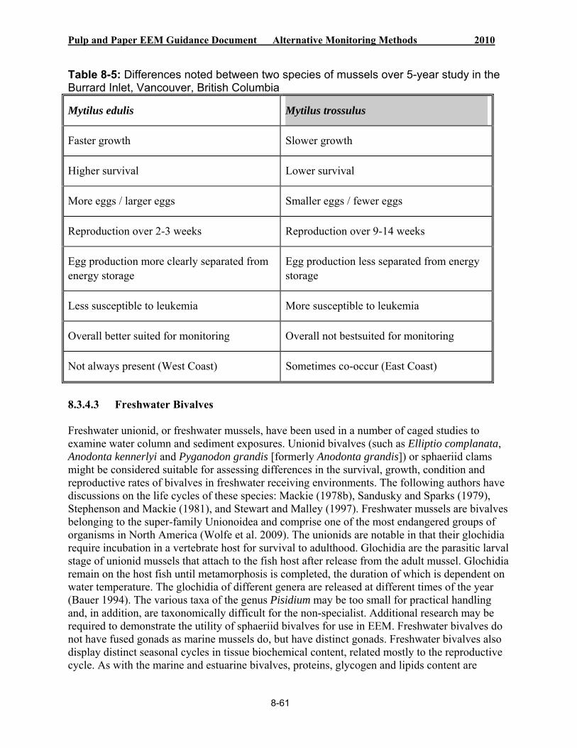
Pulp and Paper EEM Guidance Document Alternative Monitoring Methods 2010
8-61
Table 8-5: Differences noted between two species of mussels over 5-year study in the Burrard Inlet, Vancouver, British Columbia
Mytilus edulis Mytilus trossulus
Faster growth Slower growth
Higher survival Lower survival
More eggs / larger eggs Smaller eggs / fewer eggs
Reproduction over 2-3 weeks Reproduction over 9-14 weeks
Egg production more clearly separated from energy storage
s separated from energy Egg production lesstorage
Less susceptible to leukemia More susceptible to leukemia
Overall better suited for monitoring Overall not bestsuited for monitoring
Not always present (West Coast) Sometimes co-occur (East Coast)
8.3.4.3 Freshwater Bivalves
Freshwater unionid, or freshwater mussels, have been used in a number of caged studies to examine water column and sediment exposures. Unionid bivalves (such as Elliptio complanata, Anodonta kennerlyi and Pyganodon grandis [formerly Anodonta grandis]) or sphaeriid clams might be considered suitable for assessing differences in the survival, growth, condition and reproductive rates of bivalves in freshwater receiving environments. The following authors have discussions on the life cycles of these species: Mackie (1978b), Sandusky and Sparks (1979), Stephenson and Mackie (1981), and Stewart and Malley (1997). Freshwater mussels are bivalves belonging to the super-family Unionoidea and comprise one of the most endangered groups of organisms in North America (Wolfe et al. 2009). The unionids are notable in that their glochidia require incubation in a vertebrate host for survival to adulthood. Glochidia are the parasitic larval stage of unionid mussels that attach to the fish host after release from the adult mussel. Glochidia remain on the host fish until metamorphosis is completed, the duration of which is dependent on water temperature. The glochidia of different genera are released at different times of the year (Bauer 1994). The various taxa of the genus Pisidium may be too small for practical handling and, in addition, are taxonomically difficult for the non-specialist. Additional research may be required to demonstrate the utility of sphaeriid bivalves for use in EEM. Freshwater bivalves do not have fused gonads as marine mussels do, but have distinct gonads. Freshwater bivalves also display distinct seasonal cycles in tissue biochemical content, related mostly to the reproductive cycle. As with the marine and estuarine bivalves, proteins, glycogen and lipids content are

Pulp and Paper EEM Guidance Document Alternative Monitoring Methods 2010
8-62
maximal during gonad development and gametogenesis, and minimal during glochidial release. As with their marine counterparts, glycogen presents the most variation (Jadhav and Lomte 1982). Table 8-6 lists the differences between Unionoidea and Sphaeriidae.
Table 8-6: Differences noted between Unionoidea and Sphaeriidae
Unionoidea Sphaeriidae
Fast growth until maturity; then slow Slower growth; bivalve can be very small
Life span: < 6 to > 100 years Life span: 1-4 years
Fecundity: 200 000 to 17 000 000 eggs per female; small eggs
3-24 eggs per female; large eggs
Reproduction: one per year Reproduction: 3 per year, sometimes continuous
Egg production more clearly separate from energy storage
oduction less separate from energy Egg prstorage
Gonochoristic Hermaphroditic
Age at maturity: 6-12 years Age at maturity: 0.2-1 year
Less suited for studies: gonochoristic, li eroparous, often rare, difficult long- ved, int
to collect, complicated life cycles (parasitic stage)
Better suited for studies: greater abundance, ease of collection, ease of maintenance,
e span relatively simple life cycle, short lif
Bivalves should be obtained from a commercial grower when the parameter being measured is growth or chemical accumulation. Native mussels should be used for reproductive and energy parameters, preferably using a natural gradient or control impact design if the exposure period is short, or commercial mussels when the exposure period is longer. Growth should be measured using juveniles obtained from an aquaculture facility. Bivalves obtained from a commercial facility have an environmental history that is well known, and assurances of being
8.3.4.4 Source
An important consideration will be whether or not to use farmed mussels or native local mussels. Depending on the parameter being measured, there are advantages and disadvantages to both; the choice should be made in consideration of the circumstances outlined below.

Pulp and Paper EEM Guidance Document Alternative Monitoring Methods 2010
8-63
uncontaminated are greater than for animals collected in the wild. In any study, some form of species identification should be confirmed, as results may vary significantly between species, as outlined in Table 8-6. All individuals used in a caged bivalve study should be from the same population for the same parameter. If wild populations are the only possible source, they must be collected from an uncontaminated area. Epiphytic growth on bivalve shells should be removed gently by hand or with a soft brush or scraper. Collection permits for field-collected or transplanted bivalves are required by Fisheries and Oceans Canada and may be required by some local or provincial agencies. In addition, if cages present a potential obstruction to navigation, a permit may be required from the Canadian Coast Guard and a Notice to Mariners may be required. The permitting process should be considered early in the study planning process. It may take several weeks or months to process the necessary permits, as there may be a need for an environmental assessment as required by the Canadian Environmental Assessment Agency.
8.3.4.5 Species Identification
Mussels can be identified by two methods: allozyme analysis or by morphometric measurement combined with statistical analysis (McDonald et al. 1991; Mallet and Carver 1995). For the morphometric measurements, empty mussel shells are scraped to remove any remaining tissues and dried for 4-5 hours (60oC). A minimum of five shell characteristics (listed below) should be measured using a stereo microscope (6.4x magnification):
the length of the anterior adductor muscle scar; the length of the hinge plate; the distance between the anterior edge of the posterior adductor muscle scar and shell
margin; the distance between the ventral edge of the posterior adductor muscle scar and ventral
shell margin; and the distance between the pallial line and ventral shell margin midway along the shell
(Figure 8-12).
Three additional shell characteristics should be measured with callipers:
shell length; shell width; and shell height.
Each characteristic should be standardized using log10 and divided by the log10 shell length. These morphometric variables (log-transformed and length-standardized as appropriate) should then be multiplied by their raw canonical coefficients and summed to generate a canonical variate for each individual (Mallet and Carver 1995). Mytilus edulis typically has a longer anterior adductor mussel scar, a longer hinge plate, and a greater shell height than Mytilus trossulus, resulting in positive values of the standardized canonical coefficients.

Pulp and Paper EEM Guidance Document Alternative Monitoring Methods 2010
8-64
Figure 8-12: Mytilus spp. shell scars markings Note: 1) length of anterior adductor muscle scar; 2) length of hinge plate; 3) length of posterior adductor muscle scar; 4) distance between posterior edge of posterior adductor muscle scar and posterior shell margin; 5) distance between ventral edge of posterior adductor muscle scar and ventral shell margin; 6) shell width; 7) shell height. © S. St-Jean, adapted from McDonald et al. 1991.
8.3.4.6 Size and Age
All bivalves used in a caged study should belong to the same age class and be as uniform as possible in size. Typically, juvenile mussels intended for growth measurement should not have more than 5 mm difference in length at the onset of the exposure. This minimizes the number of individuals required to achieve adequate power. Juveniles are the best candidates for this parameter, as most of their energy is directed toward growth. Bivalves, and mussels in particular, have an inverse relationship between energy directed toward growth and energy directed toward reproduction. Juvenile mussels will expend most of their energy on growth with little input toward reproduction, and the ratio between growth and reproduction will slowly shift as most energy is directed to reproduction and little to growth in adults. Typically, mussels can start producing some gametes as young as 1 year old, and by 3 or 4 years old most of their energy will be directed toward reproduction and they will grow at a much slower rate. For energy and reproductive output measurement, mussels older than 3 years of age are recommended (generally at least 4 cm in length), while juveniles (between 2 and 2.5 cm) are recommended for growth.
Mussels can be aged following a combination of the techniques described in Ramon and Richardson (1992) and Sejr et al. (2002). The technique is based on annual growth bands and has been validated using a mark-and-recapture approach (Sejr et al. 2002). An experienced biologist should perform this task.

Pulp and Paper EEM Guidance Document Alternative Monitoring Methods 2010
8-65
8.3.4.7 Number of Organisms
A power analysis should be used to determine the minimum number of bivalves needed to detect a specified “effect size.” It is recommended that studies be designed to detect a 20% difference in growth. Data sets to aid in predicting the number of required organisms may be available through Environment Canada. However, when the range in mussel length is an average of 5 mm, 100 mussels will be sufficient to achieve power and to ensure an adequate number of mussels survive the exposure.
The number of animals required per cage for the growth measurements will depend on the study design (e.g., number of cages per station; see more discussion on this in the following sections), species used, age of animals, variability in response to the station, and growth conditions at the station. The number of bivalves required to fill the cages will depend on study design in terms of:
number of areas (e.g., exposure area plus number of reference areas);
number of stations per area; number of cages per mooring (if the study is designed to address varying depths in the
water column); and recommended bivalves per cage.
In addition, if tissue samples are required for tissue analysis, consideration must be given to the number of animals required to obtain a sufficient sample size for chemical analysis.
8.3.4.8 Handling and Holding Conditions
Salazar and Salazar (2000) provide detailed guidance on handling and holding conditions for bivalves, and this is summarized below. Test organisms should be handled as little as possible and should be deployed as soon as possible after collection. When handling is necessary, it should be done carefully, gently and quickly so that the bivalves are not needlessly stressed. Bivalves should be kept in well-aerated, clean-flowing water as long as possible between collection, sorting and deployment. If transporting bivalves for extended periods, keep them moist and cool by placing them in a cooler with frozen gel packs or wet ice (wet ice at the bottom of the cooler). Use seaweed or cloth towels to keep bivalves separated from the gel pack or wet ice. Newspaper should be avoided, as it contains ink that can be toxic to mussels.
8.3.5 Study Design
Determining the appropriate study design is critical if the results are going to be meaningful. The study design for caged bivalves should include a number of components:
sampling design; area and station selection; replication of cage stations and cages per station; timing and duration; modifying or confounding factors;

Pulp and Paper EEM Guidance Document Alternative Monitoring Methods 2010
8-66
supplementary measures; cage design; and mooring systems.
8.3.5.1 Sampling Design
There are six main sampling designs that are recommended for caged mussel marine and freshwater assessments:
control-impact (C-I) design; multiple control-impact (MC-I) design; simple gradient (SG) design; radial gradient (RG) design; multiple gradient (MG) design; and control–simple gradient (C-SG) design.
The C-I and MC-I designs are used to determine the magnitude of difference between homogeneous exposed and unexposed areas, while the SG, RG and MG designs examine changes in an effect along an effluent gradient. The C-I and MC-I designs are used when there are few qualitative levels of exposure. It is suggested that multiple reference areas be used rather than increasing sample sizes in one reference station. The SG, RG and MG designs may be used when there are many quantitative levels of exposure (Paine 2000); they may also be useful in discriminating among effects from sources other than pulp mill effluent. Guidance on selecting the appropriate design is provided in Chapter 2.
For example, in estuaries with complex tidal regimes and mixing regimes, an MC-I approach may be the most appropriate. An SG approach may be applicable to a river receiving environment where flow is unidirectional.
C-I, C-SG and MC-I designs require some level of replication within the control and impact areas. C-SG is a combination between C-I and SG, which is sometimes useful when more than one reference site is desired. In this case, a control, or reference station, is added to a simple gradient, typically when the far-far field does not have conditions similar to the exposed area in terms of depth or other important biotic factors. Replication at each station may not be needed for gradient designs, although an appropriate number of stations are needed in order to discriminate between spatial patterns related to effluent discharge and other spatial patterns in the environment. Replication is discussed below in section 8.3.5.2. Ultimately, it is the responsibility of study designers to develop site-specific study designs that are scientifically defensible, robust and suitably sensitive.
Pulp and Paper EEM Guidance Document Alternative Monitoring Methods 2010
8-67
8.3.5.1.1 Area and Station Selection
Chapter 2 provides guidance for the selection of multiple reference locations for a variety of receiving environments and is applicable to caged mussel studies. Reference areas should be as similar as possible to study areas in terms of the water’s:
depth; hydrodynamic conditions; temperature; salinity; dissolved oxygen concentration; and food availability and quality.
Multiple reference stations may help to identify natural differences and variability among uncontaminated areas. Often, a mixture of simple gradient and multiple control areas, such as C-SG, allows for a more robust study.
The exposure area is defined by plume characteristics. Plume delineation, as described in Chapter 2, should provide sufficient information to model average effluent concentrations with distance from source and to identify the degree of vertical mixing in the water column. This information will assist in the selection of stations and depth of deployment in the water column. More guidance is provided in the sections below.
8.3.5.2 Replication
8.3.5.2.1 Number of Cage Stations
For the exposure area, stations and depths of cage deployment may be chosen to represent a gradient of exposure to the effluent plume. The deployment stations of bivalve cages should be given careful consideration for a number of potentially interfering factors, such as the following:
In estuarine and marine situations, effluent may be positively buoyant, resulting in a thin layer of “freshwater” effluent floating on denser saline water.
In tidal situations, the mixing behaviour of effluent may be quite complex, resulting in low confidence about the average exposure concentration to which bivalves may be exposed. Tidal situations may require consideration of exposure area stations that are both “upstream” and “downstream” of the outfall.
In river discharge situations, effluent plumes may be quite long and narrow, meaning that there is little or no opportunity to meaningfully replicate cage stations within (i.e., across the long axis of) the plume.
For these and other reasons, it might be more meaningful to simply evaluate “distance from outfall” rather than effluent concentrations when designing caged bivalve studies. This approach would remain consistent with one of the objectives of EEM, which is to evaluate the magnitude and geographic extent of effects that may be related to the effluent discharge.
Pulp and Paper EEM Guidance Document Alternative Monitoring Methods 2010
8-68
The number of replicate stations must be determined to address the sampling design and EEM objectives. The number of replicate stations and sub-samples within replicate stations are determined by power analysis. The allocation and distribution of replicate stations is dependent upon the sampling design. Guidance on the use of power analysis is provided in Chapter 7. Readers are encouraged to ensure that no pseudo-replication occurs, but rather true replication. Hurlbert (1984) offers more guidance on the subject.
8.3.5.2.2 Applying Replication to Study Design
Several parameters are suggested for caged bivalve studies (survival, growth [change in length or wet weight], soft tissue fresh weight, condition, reproduction and energy storage). In order to assess these parameters on a set of bivalves exposed at different locations in the field, many different configurations of cages and bivalves are possible. For EEM studies, it may be advantageous to deploy replicate cages containing multiple bivalves at each station, and to consider only the average performance within each cage. This approach confers the additional advantage of providing redundancy in case one or more cages are lost, and may simplify the construction and deployment of cages. So long as the statistical hypothesis testing is confined to evaluating whether or not there are significant differences between areas (without uniquely attributing effects to effluent exposure), the replication and statistical analysis is valid.
As general guidance, it is suggested that cages containing 20 animals per cage be deployed for the survival measurements and at least 5 cages be deployed at each station to evaluate growth. These cages should be deployed on individual moorings, not 5 cages on one mooring, since the mooring is the most appropriate unit of statistical replication. However, practitioners should be encouraged to explore the power and robustness of potential study designs, using synthetic data (or empirical data where available) as an integral part of the study design process to determine the minimum number of animals needed.
8.3.5.3 Timing and Duration
Timing of the studies should be such that:
it coincides with a high growth period in natural populations so that growth is maximized and differences in growth rate among treatments are more measurable; and
it does not coincide with a spawning period if the test bivalves are adults.
For growth, survival and chemical accumulation, the duration of exposure should be 60-90 days (see discussion in Salazar and Salazar 2000). This should provide sufficient time for effects on survival and growth to be manifested. However, a minimum of 9 months may be needed to measure energy or reproduction; typically, on the East Coast, cages should be deployed in the summer to ensure that the energy accumulated in the fall (energy reading) is from those sites and that egg production reflects any potential effects of the effluent. Although 3 samplings are required (deployment, energy and reproduction), the cost is not generally prohibitive, as, unlike growth and survival, no measurements are needed prior to deployment.

Pulp and Paper EEM Guidance Document Alternative Monitoring Methods 2010
8-69
8.3.5.4 Modifying or Confounding Factors and Supplementary Measures
Results of caged bivalve studies will depend, at least in part, on natural factors such as temperature, food supply, other physicochemical properties of the test environments, species selected, condition of test organisms, exposure method, and handling of test organisms. Exposure and reference areas should be as similar as possible with respect to the factors listed below, to minimize confounding differences. It may be useful to measure some of the factors in order to assist in interpreting results. These factors may include life cycle, behaviour, temperature, lack of acclimation, current speed, salinity, fouling, chemical concentration and food availability. These are discussed further in Salazar and Salazar (2000).
8.3.6 Cage Designs
For growth and survival studies, cages with individual compartments are suggested so that individual bivalves can be tracked through the study. The mesh size should be maximized to allow maximum water flow but small enough to contain the test animals. Individuals are assigned to compartments such that survival, growth and condition can be tracked in each bivalve. Individual test organisms are placed in the mesh bags and separated by using a plastic cable tie or other suitable tie. Sufficient space should be allowed in each compartment to permit test animals to grow during the exposure period.
For reproduction and energy measurements, mussels do not need to be pre-measured; therefore, compartments are not necessary. However, they should still be exposed to relatively uniform conditions, and stringing mussels into socks, clumped in 3-4 individuals, is recommended (Figure 8-13). This significantly reduces the level of effort needed for this design.
A variety of cage designs are described in Salazar and Salazar (2000). A flat (i.e., two-dimensional) cage design, as shown in Figure 8-13, is suggested, as it is a convenient unit to work with. Polyvinyl chloride (PVC) tubing is a convenient material to use for constructing cages. PVC should be water-supply grade obtained from a high-quality source and soaked for at least 24 hours in flowing fresh or seawater before use to remove water-soluble and volatile chemicals. Alternative materials are described in Salazar and Salazar (2000), section 9.
Final cage dimensions depend on the size of the test organism and the number of organisms per cage. Typical bags sizes for species like mussels and clams are 10-15 cm in diameter with 5-mm mesh size. Each mesh bag should be long enough to accommodate the desired number of bivalves per bag, plus sufficient material for attachment to the PVC frame. For freshwater clam deployments, a wide variety of cage designs have been used by investigators. It is the responsibility of the study designer to ensure that cage designs are appropriate to the test species and receiving environment.
8.3.6.1 Mooring Systems
The cages can be suspended in the water column by attaching them to mooring lines that have an anchor or weight on one end (e.g., iron chain links) and a surface or subsurface buoy attached to

Pulp and Paper EEM Guidance Document Alternative Monitoring Methods 2010
Cluster of mussels in socks
Aluminum H frame
PVC Frame
8-70
Figure 8-13: Duplicate frame from a caged mussels exposure experiment © S. St-Jean
the other end (Figs. 8-14, 8-15). Salazar and Salazar (2000) discuss the factors that should be considered for deployment of cages.

Pulp and Paper EEM Guidance Document Alternative Monitoring Methods 2010
(a
(b
(c
Frames positioned vertically in water column at depth
(d
Figure 8-14: Modular mesocosm parts diagram © S. St-Jean
Juvenile mussels, pre-measured and individually separated,
Adult mussels in clumps of 3 or 4 mussels for reproduction or energy measurement
8-71

Pulp and Paper EEM Guidance Document Alternative Monitoring Methods 2010
8-72
a) Vertical View b) Plane View
Figure 8-15: Modular mesocosm flow schematic © S. St-Jean
8.3.7 Methods for Test Initiation, Cage Deployment and Retrieval and Test Termination
8.3.7.1 Test Initiation
The first step is to sort all bivalves into the desired size range(s). By selecting bivalves within a narrow size/age range, the investigator can be relatively confident that the individuals will have similar growth potential. Determining the age of wild bivalves may be difficult if not impossible for some species; length is therefore used to obtain individuals with similar growth rates.
Pulp and Paper EEM Guidance Document Alternative Monitoring Methods 2010
8-73
Commercial growers can often provide bivalves of a known age. The size range selected for test organisms depends on the species, organism supply, and target age. Test organisms should be selected within a narrow size range, and should be kept cool and moist during the sorting stage to prevent stress, damage or death (see section 8.3.4.8). For growth and survival studies, shell lengths, widths, heights and whole-animal wet weight (WAWW) are recorded for each animal and the animals assigned to individual holding containers (e.g., ice cube tray) that are labelled according to their specific location within the cage. This allows measurements of each individual test organism to be repeated at test termination. Animals in a sacrificed sub-sample (statistically appropriate number) of test organisms will be measured for shell length, WAWW, tissue weight and shell weight. For other parameters, mussels of similar size do not need to be measured; they can be placed in the socks, preferably in clumps of 3-4 individuals, as this mimics their natural clumping behaviour and minimizes stress.
For quality control purposes, approximately 20% of the measurements should be repeated and recorded by a different investigator. It is best to use an electronic spreadsheet for recording all measurements in order to reduce transcription errors. It is possible to electronically link measurement tools (e.g., vernier calipers and analytical balance) with a spreadsheet to provide an additional quality control measure.
All test organisms needed to fill the cages, plus a sub-sample for destructive sampling (tissue weight), should be sorted and measured prior to distribution among socks and cages. Test organisms are then distributed among individual mussel socks before they are attached to cages. An example of a labelling and distribution scheme is provided in Salazar and Salazar (2000), section 11.
8.3.7.2 Cage Deployment
Ensure that an appropriate vessel is chartered to assure safe transport and deployment of all cages, moorings and floats. Moorings and floats may be attached to the cages on the vessel while en route to the site. When on-site, cage location should be identified using a global positioning system (GPS) or other reliable method (e.g., nearby onshore reference points). During the exposure period, the cages may be inspected (e.g., by divers) to check for presence, damage and fouling.
8.3.7.3 Cage Retrieval and Test Termination
Cages should be retrieved using various location identifiers (e.g., GPS, depth sounders) and a grappling hook if a retrieval rope was used for each cage.
Details on test termination are provided in Salazar and Salazar (2000), section 11, and outlined here. At the processing site, bivalves from all bags for each cage should be processed together. For growth and survival measurements, it is essential that the order and orientation of each bivalve be maintained during all of the end-of-test measurements. Individuals can be removed from mesh socks and placed in labelled individual containers (e.g., ice cube trays) to facilitate measurement.

Pulp and Paper EEM Guidance Document Alternative Monitoring Methods 2010
8-74
Five to 10 minutes prior to making length and weight measurements, set the tray(s) into a tub containing clean water. Individuals that float indicate that air is trapped between the valves of the shell. When all animals in the tray(s) have opened their valves slightly and are no longer floating (5-10 minutes), length and weight measurements may begin. Start with WAWW and shell length measurements, then carefully shuck each individual and blot the tissue before taking tissue fresh-weight measurements. Note that if tissues are to be analyzed for chemical parameters, care must be taken to not introduce any contaminants from the blotting material. The Mussel Watch protocol (Gulf of Maine Council, 2001) is best suited to dissection for the purpose of chemical analysis.
8.3.8 Effect Indicators
The effect indicators to be measured in caged bivalve studies for EEM studies are survival, growth, condition and reproduction, as described in more detail below. Table 8-7 shows the effect and supporting endpoints used for a caged bivalve study. The statistical procedures are also listed and described in more detail in section 8.3.10. An example of a reporting format for recording survival and growth raw data and endpoints is provided in Table 8-8.
Table 8-7: Caged bivalve study effect indicators and endpoints and related statistical procedures
Effect Indicators
rting Effect and Suppots Endpoin
Statistical Procedure
Growth Change in size (weight and length) over time (end measurements compared to starting measurements)
WAWW Shell length and width Soft tissue fresh weight
ANOVA (regression analysis for gradient designs)
Reproduction *Mantle somatic index (MSI)y (similar to the GSI) (gonad weight against body weight)
ANOVA or ANCOVA
Condition *Weight (whole-animal dry weight, dry shell or soft tissue weight) related to shell length
Soft tissue weight related to shell weight
Soft tissue weight related to shell volume
ANOVA or ANCOVA
Survival *Percentage of individual animals alive per cage at the end of the exposure period
Length frequency analysis
ANOVA
* Caged bivalve effect endpoints used for determining effects. Other supporting endpoints can be used to support analyses.

Pulp and Paper EEM Guidance Document Alternative Monitoring Methods 2010
8-75
y Currently, guidance is only provided on the relative mantle somatic index (similar to the gonad index [GSI]). See section 8.3.8.5.
8.3.8.1 Survival
Survival is not a particularly sensitive indicator of effects in caged bivalves, but it is an important parameter to monitor. Survival can be easily determined and quantified, although it is possible to have some individuals missing at the test end due to shell decomposition. Bivalves are dead if they are gaping open and do not close their shells when touched or tapped. Survival is expressed as percent of individual animals alive per cage at the end of the exposure period.
8.3.8.2 Growth
Growth is a measure of energy use and is a sensitive indicator of effects that is easy to measure. Several types of growth measurements should be made; measuring only one could provide misleading results. Growth measurements, with their expected accuracy, are measured at test initiation and termination as outlined below:
WAWW ± 0.001 g Shell length ± 0.01 mmShell width ± 0.01 mmShell height ± 0.01 mm
Growth can be expressed in a number of ways:
absolute growth = absolute change in value from test initiation to test termination;
growth rate = absolute change in value per unit of time, typically using one week as the time increment; or
relative growth = (final weight – initial weight) / initial weight; relative growth may be used when there is a significant difference among cages in initial weights; relative growth is expressed as a proportion and therefore an arcsin square root transformation of relative growth values may be appropriate prior to applying statistics. Green (1979) provides useful advice on this transformation, noting that it is not usually required for proportion data in the range of 0.3-0.7, and that while it may not always help, it probably does no harm, either.
Use the most appropriate expression of growth to suit the study design and site-specific characteristics.
8.3.8.3 Condition
Condition is a measure of how an animal stores its energy, and it can be measured in both adults and juvenile mussels. There is more than one option that may be considered for calculating condition, as described below. Note that some of these methods require measurement of variables that are in addition to those outlined in section 8.3.8.2. The most appropriate method to calculate condition is left to the discretion of the investigators.

Pulp and Paper EEM Guidance Document Alternative Monitoring Methods 2010
8-76
Weight (whole-animal dry weight, dry shell or soft tissue weight) related to shell length: This is analogous to the Fulton Condition Index (Ricker 1975; Anderson and Neumann 1996) used in fisheries biology. This relationship may be characterized according to a conventional formula for a straight line (e.g., in Mackie and Flippance 1983), with slope (C) and intercept (b):
log W = b + (C log L)
High values of C imply that a bivalve has a relatively high tissue weight at a given length, whereas low values may indicate that an animal is not obtaining sufficient food or is experiencing chronic stress that prevents it from thriving. This method of characterizing condition is suitable for assessing condition in wild bivalves where shell length is expected to be quite variable. However, since animals used for caged bivalve studies are screened for uniform length at test initiation, this method will not be reliable. This method may also not be suitable for bivalves because shell length and tissue weight are influenced by different factors in the environment (Salazar, personal communication).
Soft tissue weight related to shell weight: This method of characterizing condition uses soft tissue weight and shell weight. An ANOVA can be conducted or, more simply, soft tissue weight can be divided by shell weight. Grout and Levings (2000) measured the condition of Blue Mussels as the ratio of tissue weight to shell weight. They found that condition distinguished caged mussels in a high survival zone (condition index 1.10 to 1.42) from caged mussels in a low survival zone (condition index 0.82 to 0.96).
Soft tissue weight related to shell volume: This method was used by Mucklow (1996; based on Seed 1968) to calculate condition by dividing soft tissue dry weight by shell volume, measured as length x width x height. In a study on wild Blue Mussel populations, Mucklow (1996) concluded that seasonal patterns in condition index were variable and influenced by a number of natural factors, including food availability and physiological energy requirements.
8.3.8.4 Energy Measure
As seen in Figure 8-11, energy accumulation also occurs in the mantle, and has an annual cycle. Generally, Blue Mussels will reach their maximal energy content in late fall. When the mantle is at that stage, most of the weight consists of stored glycogen that will be used later for reproduction. Prior to dissection, mussels should be assessed for WAWW and shell measurements (length, weight, height and internal scarring). Mantle lobes should be separated from the body and weighed (mantle wet weight), after which the weight of the remainder of the body should be added to determine the body wet weight. Samples should be dried at 55°C until a constant weight is reached (approximately 2-3 days). Mantle dry weight and body dry weight should both be measured, from which the LSI-like measure can be derived. The bivalve LSI consists of the ratio of the dry weight of the mantle to the dry weight of the animal.

Pulp and Paper EEM Guidance Document Alternative Monitoring Methods 2010
8-77
A) B)
Figure 8-16: A) Mantle plug and tools necessary for its removal; B) Mantle plug after homogenization and ready for assessment © S. St-Jean
8.3.8.5 Reproductive Effort
Recent research has found that the MSI for mussels, similar to the GSI in fish, can be used to determine reproductive investment. Most of the gametes produced by the mussel are stored in the mantle lobes. The following is a summary of steps to determine the MSI of mussels:
1. Measure the mussel length, width, height and the whole animal weight. 2. Dissect each mussel. 3. Determine the sex. 4. Remove and weigh each mantle lobe and determine the body mass of each individual. 5. If female: one mantle lobe should be used for dry weight and calculation of GSI ratio (ratio
of body weight [minus gonads] to gonad). If male, both lobes are used. Female calculation should be extrapolated for both lobes.
6. The second lobe should be used to assess reproductive effort, through egg measurement and count.
7. Calculate the MSI (ratio of body weight [minus gonads] to gonad).
The MSI should be determined when 90% of the mantle lobe consists of gonads. There are numerous factors to consider that will affect the time of spawning: water depth, seasonal temperature, response patterns, and prevalence of different species. Boudreau et al. (in preparation), and St-Jean et al. (2008) conducted studies using MSI on the Atlantic and Pacific coasts of Canada, using different species. They found that Bay Mussels from the Pacific coast did not have a characteristic peak in gamete production preceding spawning, unlike the Blue Mussels from the Atlantic coast. Boudreau et al. (in preparation) also assessed reproductive effort by calculating and weighing the number of eggs in each mantle.
For more detailed information on the MSI, please refer to St-Jean (2003), or contact a regional EEM program coordinator for further information and complete techniques.

Pulp and Paper EEM Guidance Document Alternative Monitoring Methods 2010
8-78
Briefly, the supplemental technique consists of the following (Fig. 8-16):
1. Weigh gonad lobe on analytical balance. 2. Extract a small plug of tissue using the straws provided. 3. Weigh the plug. 4. Mince the plug. 5. Using the microscope ocular grid at a magnification of 400x, measure 20 eggs
(measurements are of the whole egg and nucleus). 6. Count representative sub-samples in a counting chamber. 7. Repeat Step 6, 2 more times, for a total of 3 counts.
Table 8-8: An example of a field data sheet for recording survival and growth raw data*
Caged Bivalve Field Data Sheet
Site Station Biologist Comments:
Date received Date processed Chemical analysis required? Date shipped Sample weight (chemistry)
Storage
To:
Animal No.
Length (L) (mm)
Height (H) (mm)
Width (W) (mm)
WAWW (g)
Mantle wet weight (WW) (g)
Whole -Animal Dry Weight (g)
Mantle dry weight (DW) (g)
Dry Shell Weight(g)
1 2 3 4 5 6 7 8 9 10 11 12 13 14 15 16 17 18 19

Pulp and Paper EEM Guidance Document Alternative Monitoring Methods 2010
_____ ____ _________
________________ _____________________________
8-79
Site Station Biologist Comments:
Date received Date processed Chemical analysis required? Date shipped Sample weight (chemistry)
Storage
To:
Animal No.
Length (L) (mm)
Height (H) (mm)
Width (W)(mm)
WAWW(g)
Mantle wet weight (WW) (g)
Whole -Animal Dry Weight (g)
Mantle dry weight (DW) (g)
Dry Shell Weight(g)
20 QA/QC
Number of mussels alive at end of test Percent survival
Site Conditions:
Date Time Temperature (C )
Dissolved Oxygen (mg/L)
Salinity (parts per thousand)
urrent Celocity V
(cm/sec)
Current Direction (degrees)
Field Staff:
Notes:
* Data sheet provided by SSJ Environmental Limited
8.3.9 Quality Assurance and Quality Control
All work should be performed by suitably qualified and trained staff (biologists and technicians). Where contractors are used they should be selected for their specialist expertise. All fieldwork should be carried out following standard operating procedures to ensure overall consistency and that appropriate procedures are followed. All field and laboratory measurements should be made using properly calibrated instruments. All field data should be recorded using standard forms to ensure that all of the required data are collected in a reproducible and standardized format.
Pulp and Paper EEM Guidance Document Alternative Monitoring Methods 2010
8-80
Replicate measures should be taken on 20% of all measures in order to verify the accuracy and reproducibility of both field measurements and laboratory analyses. For mussels in socks, this represents at least two mussels per sock.
In data analysis, the first step should be the screening of the data for outliers. A rapid way to screen for outliers is to create scatter plots of pairs of variables with 95% confidence ellipses superimposed. Potential outlier data points can then be identified as those that lie outside the confidence ellipses. Outliers can be the result of a number of causes, including data entry or transcription errors. Where outliers are detected, the data records should be reviewed in order to isolate and if possible correct the source of a potential error. Where no such identification is possible, the analysis should be performed both with and without the outlier, in order to evaluate the influence that the outlier exerts on the results of the data analysis.
Statistical data will be examined to evaluate the degree to which they conform to the underlying assumptions of the analysis (such as normality and homogeneity of variance, or equality of slopes in ANCOVA). Where appropriate, transformations may be applied in order to lessen the magnitude of violations of the underlying assumptions.
8.3.10 Data Analyses
Data analyses and interpretation of the results should be appropriate to the study design. Caged mussel studies for EEM are designed to determine if there are significant effects on biota in the vicinity of effluent outfalls. This can be accomplished by using a C-I (= reference − exposure) or a gradient (= regression) type of design. Statistical procedures appropriate to each effect indicator (i.e., survival, growth, reproduction, energy and condition) are summarized in Table 8-7.
An ANCOVA should be performed to test the GSI (dry gonad weight), condition (dry body weight) with covariates to remove influences including dry body weight for GSI, and shell length for condition. Where an interaction between treatment and covariate precludes the use of an ANCOVA, stratified subsets of the covariate should be compared in a single-factor ANOVA. When the control groups are not significantly different, they should be grouped for the analyses. However, if a significant difference is found between groups, all controls should be included in the analyses. A Tukey multiple-comparison test can be employed when significant differences are found among groups. Non-normality (probability plot) or heteroscedasticity (Fmax test) that cannot be resolved by appropriate data transformations should be followed by non-parametric analysis using the Kruskal-Wallis test, followed by a Noether multiple-comparison test (Scherrer 1984; Zar 1999). Probit analysis can be employed for survival. The level of significance should be set at p < 0.05, and back-transformed means should be accompanied by their 95% confidence interval.
The first step is to generate summary statistics for each parameter (i.e., WAWW, shell length, soft tissue fresh weight) and each cage and station.
The second step is to determine whether there are significant differences among replicate cages for each of the parameters measured before deployment (if they were not measured

Pulp and Paper EEM Guidance Document Alternative Monitoring Methods 2010
8-81
post-distribution and before deployment). This involves assessing the data for normality and homogeneity of variances.
The final step is to use the appropriate statistical test for the study design. In general, ANOVA and multiple-comparison tests are used for hypothesis testing and comparison among stations. For C-I and MC-I designs using ANOVA and ANCOVA procedures, detailed guidance is provided in Chapter 7 of this guidance document. If statistical differences are found, a multiple-range test, or its non-parametric counterpart, can be used to determine which stations are different from the others. Linear and multiple-regression analyses (using variables regressed on distance) may generally be used to establish relationships among variables along exposure gradients. For ANCOVA analyses of condition, the covariates will be dictated by the condition formula that is used.
8.3.11 Dioxins and Furans
If a mill is required to measure dioxins and furans in fish tissue, measuring these chemicals in caged bivalves may be considered. However, there are some precautions that should be taken with this approach, including the following:
Duration of exposure should be chosen such that dioxins and furans are likely to be accumulated to detectable levels in bivalve tissue.
Consider whether bivalves would be harvested (commercially or recreationally) for human consumption in the area.
Ensure that the number of bivalves included in the design is sufficient to obtain enough tissue for analysis.
There may be mills for which caged bivalves would not be considered suitable for measuring uptake of dioxins and furans. Any proposal to use caged bivalves for dioxin and furan measurements would require approval by the Regional Authorization Officer. 8.3.12 Reporting
QA/QC considerations for caged bivalve studies should follow those outlined for the fish survey in Chapter 3 of this guidance document. QA/QC measures apply to the following components of caged bivalve studies:
study design; field sampling; sample processing / laboratory analysis; data analysis; and reporting.
8.4 References

Pulp and Paper EEM Guidance Document Alternative Monitoring Methods 2010
8-82
Anderson RO, Neumann RM. 1996. Length, weight, and associated structural indices. In Murphy BR, Willis DW, editors. Fisheries techniques. 2nd edition. Bethesda (MD): American Fisheries Society. p. 447-482.
Andrews S, Parker R. 1999. Draft Report (II). An environmental quality evaluation of Pictou Harbour, Nova Scotia, using caged bivalves; Mytilus edulis. Prepared by Environmental Protection Branch of Environment Canada, Dartmouth (NS) for the Pictou Harbour Environmental Protection Project, New Glasgow (NS).
Ankley GT, Jensen KM, Kahl MD, Korte JJ, Makynen EA. 2001. Description and evaluation of a short-term reproduction test with the fathead minnow (Pimephales promelas). Environ Toxicol Chem 20:1276-1290.
Ankley GT, Jensen KM, Makynen EA, Kahl MD, Korte JJ, Hornung MW, Henry TR, Denny JS, Leino RL, Wilson VS, et al. 2003. Effects of the androgenic growth promoter 17-beta-trenbolone on fecundity and reproductive endocrinology of the fathead minnow. Environ Toxicol Chem 22:1350-1360.
Applied Biomonitoring. 2000. Caged Mussel Pilot Study Port Alice Mill, Vancouver Island. EEM Program. Environment Canada, Environmental Protection Branch, Pacific and Yukon Region. Regional Manuscript Report MS 00-01.
Atz JW. 1986. Fundulus heteroclitus in the laboratory: a history. Amer Zool 26:111-120.
Barber WE, Kevern NR. 1974. Seasonal variation of sieving efficiency in a lotic habitat. Freshwat Biol 4:293-300.
Bauer G. 1994. The adaptive value of offspring size among freshwater mussels (Bivalvia; Unionoidea). J Anim Ecol 63:933–944.
Beckvar N, Salazar S, Salazar M, Finkelstein K. 2000. An in situ assessment of mercury contamination in the Sudbury River, Massachusetts, using transplanted freshwater mussels (Elliptio complanata). Can J Fish Aquat Sci 57:1103-1112.
Bothwell ML. 1985. Phosphorus limitation of lotic periphyton growth rates: an intersite comparison using continuous-flow troughs (Thompson River system, British Columbia). Limnol Oceanogr 30:527-542.
Bothwell ML, Daley RJ. 1981. Determination of phosphorus sufficiency and growth rates of benthic algae in the Thompson River, BC, using experimental flowing troughs. IWD Regional Report. Vancouver (BC): Inland Waters Directorate, Environment Canada.
Bothwell ML, Derksen G, Nordin RN, Culp JM. 1992. Nutrient and grazer control of algal biomass in the Thompson River, British Columbia: a case history of water quality management,. In Robarts RD, Bothwell ML, editors. Aquatic ecosystems in semi-arid regions: implications for resource management. (National Hydrology Research Institute Symposium Series 7). Saskatoon (SK): Environment Canada. p. 253-266.

Pulp and Paper EEM Guidance Document Alternative Monitoring Methods 2010
8-83
Bothwell ML, Culp JM. 1993. Sensitivity of the Thompson River to phosphorus: studies on trophic dynamics. NHRI Contribution No. 93006.Saskatoon (SK): National Hydrology Research Institute, Environment Canada.
Burt A, Kramer DL, Nakasuru K, Spry C. 1988. The tempo of reproduction in Hyphessobrycon pulchripinnis (Characidae), with a discussion on the biology of “multiple spawning”. Environ Biol Fish 22:15-27.
Carlisle DM. 2000. Bioenergetic food webs as a means of linking toxicological effects across scales of ecological organization. J Aquat Eco Stress Rec 7:155-165.
Dubé MG, Culp JM, Cash KJ, Glozier NE, MacLatchy DL, Podemski CL, Lowell RB. 2002. Artificial streams for environmental effects monitoring (EEM): development and application in Canada over the past decade. Wat Qual Res J Can 37(1):155-180.
Chen CY, Stemberger RS, Klaue B, Blum JD, Pickhardt PC, Folt CL. 2000. Accumulation of heavy metals in food web components across a gradient of lakes. Limnol Oceanogr 45:1525-1536.
Clarke A. 1973. The freshwater molluscs of the Canadian Interior Basin. Malacologia 13:1-509.
Clarke A. 1981. The freshwater molluscs of Canada. Ottawa (ON): National Museums of Canada.
Coad BW. 1995. Encyclopedia of Canadian fishes. Waterdown (ON): Canada Museum of Nature and Canadian Sportfishing Productions Inc.
Couillard Y, Campbell PGC, Tessier A, Pellerin-Massicotte J, Auclair JC. 1995 a. Field transplantation of a freshwater bivalve, Pyganodon grandis, across a metal contamination gradient. I. Temporal changes in metallothionein and metal (Cd, Cu, and Zn) concentrations in soft tissues Can J Fish Aquat Sci 52:690-702.
Couillard Y, Campbell PGC, Tessier A, Pellerin-Massicotte J, Auclair JC. 1995b. Field transplantation of a freshwater bivalve, Pyganodon grandis, across a metal contamination gradient. II. Metallothionein response to Cd and Zn exposure, evidence for cytotoxicity, and links to effects at higher levels of biological organization. Can J Fish Aquat Sci 52:703-715.
Courtenay SC, Parker WR, Rawn GP. 1998. Proceedings of a workshop to assess alternatives to the fish survey component of the environmental effects monitoring program for Canadian pulp and paper mills. (Canadian Technical Report of Fisheries and Aquatic Sciences 2233).
Crane M, Burton GA, Culp JM, Greenberg MS, Munkittrick KR, Ribeiro R, Salazar M, St-Jean S. 2007. In situ approaches for stressor and effect diagnosis. Integr Environ Assess Manag 3:234-245.
Culp JM, Cash KJ. 1995. Potential impacts of effluent on the Thompson and upper Fraser Rivers. DOE FRAP 1995-10. Vancouver (BC): Fraser River Action Plan, Environmental Conservation Branch, Environment Canada.

Pulp and Paper EEM Guidance Document Alternative Monitoring Methods 2010
8-84
Culp JM, Podemski CL. 1996. Design and application of a novel stream microcosm system for assessing effluent impacts to large rivers. In Servos MR, Munkittrick KR, Carey JH, Van Der Kraak GJ, editors. Environmental fate and effects of pulp and paper mill effluents. Delray Beach (FL): St. Lucie Press. p. 549-555.
Culp JM, Podemski CL, Cash KJ, Lowell RB. 1996. Utility of field-based artificial streams for assessing effluent effects on riverine ecosystems. J Aquat Ecosystem Health 5:117-124.
Culp JM, Lowell RB. 1998. Pulp mill effluent impacts on benthic communities and selected fish species in the Fraser River Basin. In Gray C, Tuominen T, editors. Health of the Fraser River aquatic ecosystem, Vol. II. DOE FRAP 1998-11. Ottawa (ON): Environment Canada. p. 13-34.
Culp JM, Lowell RB, Cash KJ. 2000a. Integrating mesocosm experiments with field and laboratory studies to generate weight-of-evidence risk assessments for large rivers. Environ Toxicol Chem 19:1167-1173.
Culp JM, Podemski CL, Cash KJ, Lowell RB. 2000b. A research strategy for using stream microcosms in ecotoxicology: integrating experiments at different levels of biological organization with field data. J Aquat Eco Stress Rec 7:167-176.
Culp JM, Podemski CL, Cash KJ. 2001. Interactive effects of nutrients and contaminates from pulp mill effluents on riverine benthos. J Aquat Eco Stress Rec 8(1):67-75.
Culp JM, Glozier NE, Cash KJ, Dubé MG, Waiser M, MacLatchy DL, Brua B, Firth B, Wilson G. 2004. Cumulative effects investigation of pulp mill and sewage effluent impacts on benthic food webs: a mesocosm example. In Borton DL, Hall TJ, Fisher RP and Thomas JF, editors. Pulp and paper mill effluent environmental fate and effects, proceedings of the Fifth International Conference on Fate and Effects of Pulp and Paper Mill Effluents, June 1-4, 2003, Seattle, Washington, USA. Lancaster (PA): DEStech Publications. p. 464-472.
Day KE, Metcalfe JL, Batchelor SP. 1990. Changes in intracellular free amino acids in tissues of the caged mussel (Elliptio complanata), exposed to contaminated environments. Arch Environ Cont Toxicol 19:816-827.
Drake JA, Huxel GR, Hewitt CL. 1996. Microcosms as models for generating and testing community theory. Ecology 77:670-677.
Dubé MG. 1995. Effects of bleached kraft pulp mill effluent on periphyton and chironomid abundance in the Thompson River, British Columbia [master’s thesis]. Saskatoon (SK): University of Saskatchewan.
Dubé MG. 2000. Sources of contaminants in the bleached kraft pulping process and their effect on the mummichog (Fundulus heteroclitus) [dissertation]. Saint John (NB): University of New Brunswick.
Dubé MG, Culp JM. 1996. Growth responses of periphyton and chironomids exposed to biologically treated bleached kraft pulp mill effluent. Environ Toxicol Chem 15:2019-2027.

Pulp and Paper EEM Guidance Document Alternative Monitoring Methods 2010
8-85
Dubé MG, Culp JM, Scrimgeour GJ. 1997. Nutrient limitation and herbivory: processes influenced by bleached kraft pulp mill effluent. Can J Fish Aquat Sci 54:2584-2595.
Dubé MG, MacLatchy DL. 2000a. Endocrine responses of an estuarine fish Fundulus heteroclitus to final effluent from a bleached kraft pulp mill before and after installation of reverse osmosis treatment of a waste stream. Environ Toxicol Chem 19:2788-2796.
Dubé MG, MacLatchy DL. 2000b. Reverse osmosis treatment of condensates from a bleached kraft pulp mill: effects on acute and chronic toxicity of process streams and final effluent. In Ruoppa M, Paasivirta J, Lehtinen K-J, Ruonala S, editors. Proceedings of the Fourth
International Conference on Environmental Impacts of the Pulp and Paper Industry. Helsinki (FI). p. 270-276.
Dubé MG, MacLatchy DL. 2001. Identification and treatment of a waste stream at a bleached kraft pulp mill that depresses a sex steroid in the mummichog (Fundulus heteroclitus). Environ Toxicol Chem 20:985-995.
Dubé MG, Culp JC, MacLatchy DL, Gillis G, Parker R, Courtenay S, Gilman G. 2002. Utility of mobile, field-based artificial streams for assessing effects of pulp mill effluents on fish in the Canadian Environmental Effects Monitoring (EEM) program. J Aquat Eco Stress Rec 9:85-102.
Dubé MG, MacLatchy DL, Firth BK, Culp JM, Glozier NE, Cash KJ. 2004. Using mesocosms to explore confounding factors influencing longnose dace (Rhinichthys cataractae) responses to kraft mill effluent on the Wapiti River, AB, Canada. In Borton DL, Hall TJ, Fisher RP, Thomas JF, editors. Pulp and paper mill effluent environmental fate and effects, Proceedings of the Fifth International Conference on Fate and Effects of Pulp and Paper Mill Effluents, June 1-4, 2003, Seattle, Washington, USA. Lancaster (PA): DEStech Publications. p. 481-490.
Dubé MG, MacLatchy DL, Kieffer JD, Glozier NE, Culp JM, Cash KJ. 2005. Effects of metal mining effluent on Atlantic salmon (Salmo salar) and slimy sculpin (Cottus cognatus): using mesocosms to assess existing effects and predict future consequences. Sci Total Environ 343:135-154.
Dubé MG, MacLatchy DL, Hruska KA, Glozier NE. 2006. Assessing the responses of creek chub (Semotilus atromaculatus) and pearl dace (Semotilus margarita) to metal mine effluents using in situ artificial streams in Sudbury, Ontario, Canada. Environ Toxicol Chem. 25(1):18-28.
Environment Canada. 1997. Fish Survey Working Group Final Report. Recommendations from Cycle 1 Review. Ottawa (ON): National EEM Office, Science Policy and Environmental Quality Branch, Environment Canada. EEM/1997/6.
Federal-Provincial Thompson River Task Force. 1976. Sources and effects of algal growth, colour, foaming and fish tainting in the Thompson River system. Victoria (BC): Environmental Protection Division, British Columbia Ministry of Environment, Lands and Parks.
Freeman KR, PerryKL, DiBaccoTG, Scarratt DJ. 1994. Observations on two Mytilid species from a Nova Scotian mussel farm. (Canadian Technical Report of Fisheries and Aquatic Sciences 1969). Halifax (NS): Fisheries and Oceans Canada.

Pulp and Paper EEM Guidance Document Alternative Monitoring Methods 2010
8-86
Fritz ES, Meredith WH, Lotrich VA. 1975. Fall and winter movements and activity level of the mummichog Fundulus heteroclitus, in a tidal creek. Chesapeake Sci. 16:211-215.
Gibbons WN, Munkittrick KR, Taylor WD. 1998a Suitability of small fish species for monitoring the effects of pulp mill effluent on fish. 1. Response of spoonhead sculpin exposed to bleached kraft mill effluent. Environ Toxicol Chem 7(11):2227-2237.
Gibbons WN, Munkittrick KR, Taylor WD. 1998b. Suitability of small fish species for monitoring the effects of pulp mill effluent on fish. 2. Comparison of trout perch responses to white sucker exposed to bleached kraft mill effluent. Environ Toxicol Chem 17(11):2238-2245.
Goldberg ED, Bowen VT, Farrington JW, Harvey G, Martin JH, Parker PL, Risebrough RW, Robertson W, Schneider E, Gamble E. 1978. The Mussel Watch. Environ Conserv 5(2):101-125.
Gray C, Tuominen T. 1998. Health of the Fraser River aquatic ecosystem, Vol. I. DOE FRAP 1998-11. Vancouver (BC): Environment Canada.
Green RH. 1979. Sampling design and statistical methods for environmental biologists. Toronto (ON): John Wiley & Sons.
Grout JA, Levings CD. 2000. Effects of acid mine drainage from an abandoned copper mine, Britannia Mines, Howe Sound, British Columbia, Canada, on transplanted blue mussels (Mytilus edulis). Mar Environ Res 51(3):265-288.
Gulf of Maine Council on the Marine Environment. 1997. Gulfwatch Project: standard procedures: filed and laboratory. Gulfwatch implementation period 1993-2001. August 1997.
Harries JE, Runnals T, Hill E, Harris CA, Maddix S, Sumpter JP, Tyler CR. 2000. Development of a reproductive performance test for endocrine disrupting chemicals using pair breeding fathead minnows (Pimephales promelas). Environ Sci Technol 34:3003-3011.
Heins DC, Rabito FG Jr. 1986. Spawning performance in North American minnows: direct evidence of the occurrence of multiple clutches in the genus Notropis. J Fish Biol 28:343-357.
Hinch SG, Kelly LJ, Green RH.1989. Morphological variation of Elliptio complanata (Bivalvia: Unionidae) in differing substrata of soft-water lakes exposed to acidic deposition. Can J Zool 67:1895-1899.
Hornbach DJ, Wissing TH, Burky AJ. 1982. Life-history characteristics of a stream population of the freshwater clam Sphaerium striatinum Lamarck (Bivalvia: Pisidiidae). Can J Zool. 60:249-260.
Hruska K, Dubé MG. 2004. Using artificial streams to assess the effects of metal-mining effluent on the life-cycle of the freshwater midge (Chironomus tentans) in situ. Environ Toxicol Chem 23(11):2709-2718.
Hruska K, Dubé M. 2005. Comparison of a partial life cycle bioassay in artificial streams to a standard beaker bioassay to assess effects of metal mine effluent on Chironomus tentans.

Pulp and Paper EEM Guidance Document Alternative Monitoring Methods 2010
8-87
Environ Toxicol Chem 24(9):2325-2335.
Hurlbert SH. 1984. Pseudoreplcation and the design of ecological field experiments. Ecol Monog 54:187-211.
Jadhav ML, Lomte VS. 1982. Seasonal variation in biochemical composition of the freshwater bivalve, Lamellidens corrianus. Rivista di Idrobiologia. 21:1-7.
Jenkin, RE, Burkhead NM. 1993. Freshwater fishes of Virginia. Bethesda (MD): American Fisheries Society.
Jensen KM, Korte JJ, Kahl MD, Pasha MS, Ankley GT. 2001. Aspects of basic reproductive biology and endocrinology in the fathead minnow (Pimephales promelas). Comp Biochem Physiol Part C. 128:127-141.
Jensen KM, Kahl MD, Makynen EA, Korte JJ, Leino RL, Butterworth BC, Ankley GT. 2004. Characterization of responses to the antiandrogen flutamide in a short-term reproduction assay with the fathead minnow. Aquat Toxicol 70:99-110.
Jernelov A. 1996. The International Mussel Watch: A global assessment of environmental levels of chemical contaminants. Sci Tot Environ 188 (Suppl. 1): 37-44.
Kneib RT. 1986. The role of Fundulus heteroclitus in salt marsh trophic dynamics. Amer Zool 26:259-269.
Kneib RT, Stiven AE. 1978. Growth, reproduction, and feeding of Fundulus heteroclitus (L.) on a North Carolina salt marsh. J Exp Mar Biol Ecol 31:121-140.
Leblanc J, Couillard CM. 1995. Description de la période de reproduction d’un poisson sentinelle: le choquemort (Fundulus heteroclitus) de l’estuaire de la Miramichi. (Rapport technique canadien des sciences halieutiques et aquatiques 2057). Mont-Joli (QC): Fisheries and Oceans Canada.
Lowell RB, Culp JM, Wrona FJ. 1995. Stimulation of increased short-term growth and development of mayflies by pulp mill effluent. Environ Toxicol Chem 14:1529-1541.
Lowell RB, Culp JM, Wrona FJ, Bothwell ML. 1996. Effects of pulp mill effluent on benthic freshwater invertebrates: food availability and stimulation of increased growth and development. In Servos MR, Munkittrick KR, Carey JH, Van Der Kraak GJ, editors. Environmental fate and effects of pulp and paper mill effluents. Delay Beach (FL): St. Lucie Press. p. 525-532.
Lowell RB, Culp JM, Dubé MG. 2000. A weight-of-evidence approach for northern river risk assessment: integrating the effects of multiple stressors. Environ Toxicol Chem 19:1182-1190.
Mackie GL. 1978a. Shell structure in freshwater Sphaeriaceae. (Bivalvia: Heterondonta). Can J Zool 56:1-6.
Mackie GL. 1978b. Are sphaeriid clams ovoviviparous or viviparous? Nautilus 92:145-147.

Pulp and Paper EEM Guidance Document Alternative Monitoring Methods 2010
8-88
Mackie GL, Quadri SU, Clarke AH. 1974. Development of brood sacs in Musculium securis Bivalvia: Sphaeriidae. Nautilus 88:109-111.
Mackie GL, Flippance LA. 1983. Growth dynamics in Sphaerium rhomboideum (Bivalvia: Pisidiidae). Can J Zool 61:868-873.
Mallet AL, Carver CE. 1995. Comparative growth and survival patterns of Mytilus trossulus and Mytilus edulis in Atlantic Canada. Can J Fish Aquat Sci 52:1873-1880.
Malley DF, Stewart AR, Hall BD. 1996. Uptake of methyl mercury by the floater mussel, Pyganodon grandis (Bivalvia, Unionidae), caged in a flooded wetland. Environ Toxicol Chem 15:928-936.
Martel P, Kovacs T, Voss R. 2003. Survey of pulp and paper mill effluents for their potential to affect fish reproduction. Proceedings of the Fifth International Conference on the Fate and Effects of Pulp and Paper Mill Effluents, Seattle, Washington, USA, June 1-4, 2003. p. 78-91.
Mason RP, Laporte JM, Andres S. 2000. Factors controlling the bioaccumulation of mercury, methylmercury, arsenic, selenium and cadmium by freshwater invertebrates and fish. Arch Environ Contam Toxicol 38:283-297.
McDonald JH, Seed R, Koehn RK. 1991. Allozymes and morphometric characteristics of three species of Mytilus in the northern and southern hemispheres. Mar Biol 11:323-333.
McGreer ER, Belzer W. 1998. Contaminant sources. In Gray C, Tuominen T, editors. Health of the Fraser River aquatic ecosystem, Vol. I. DOE FRAP 1998-11. Ottawa (ON): Environment Canada. p. 7-22.
McMahon RF. 1991. Mollusca: bivalvia. In Thorp JH, Covich AP, editors. 1991. Ecology and classification of North American freshwater invertebrates. San Diego (CA): Academic Press. p. 315-399.
Metcalfe-Smith JL, Green RH, Grapentine LC. 1996. Influence of biological factors on concentrations of metals in the tissues of freshwater mussels (Elliptio complanata and Lampsilis radiata radiata) from the St. Lawrence River. Can J Fish Aquat Sci 53:205-219.
Mucklow LC. 1996. Effects of season and species on physiological condition and contaminant burdens in mussels (Mytilus edulis L. and Mytilus trossulus G.): implications for mussel watch programs [master’s thesis]. Halifax (NS): School for Resource and Environmental Studies, Dalhousie University.
Nelson JS, Paetz MJ. 1992. The fishes of Alberta. Calgary (AB): University of Calgary Press.
Newell RIE. 1989. Species profile of the blue mussel, Mytilus edulis. US Fish Wildl Ser Biol Rep 82(11):40.
Ni IH, Wang WX, Tam YK. 2000. Transfer of Cd, Cr and Zn from zooplankton prey to

Pulp and Paper EEM Guidance Document Alternative Monitoring Methods 2010
8-89
mudskipper Periophthalmus cantonensis and glassy Ambassis urotaenia fishes. Mar Ecol-Prog Ser 194:203-210.
O’Connor. 1992. Recent trends in coastal environmental quality: Results from the first five years of the NOAA Mussel Watch Project. Washington (DC): U.S. Department of Commerce, National Oceanic and Atmospheric Administration (NOAA), and National Ocean Service.
[OECD] Organisation for Economic Co-operation and Development. 2001. Detailed review paper: appraisal of test methods for sex hormone disrupting chemicals. (OECD Series on testing and assessment 21). ENV/JM/MONO(2002)8.
[OECD] Organisation for Economic Co-operation and Development. 2006. Report of the validation of the 21-day fish screening assay for the detection of endocrine substances (Phase 1B). (OECD Series on testing and assessment 61). ENV/JM/MONO(2006)29.
Paine MD. 1990. Life history tactics of darters (Percidae: Etheostomatiini) and their relationship with body size, reproductive behaviour, latitude and rarity. J Fish Biol 37:473-488.
Paine MD. 2000. EEM Design. Short-Course presented at the 27th Annual Aquatic Toxicity Workshop, October 1-4th, St. John’s, NF.
Panter GH, Hutchinson TH, Lange R, Lye CM, Sumpter JP, Zerulla M, Tyler CR. 2002. Utility of a juvenile fathead minnow screening assay for detecting (anti-)estrogenic substances. Environ Toxicol Chem 21(2):319-326.
Parker R, Smith N. 1997. A synopsis of the results of environmental effects monitoring studies at 19 pulp and paper mills in Atlantic Canada. In Proceedings of the Third International Conference on Environmental Effects of Pulp and Paper Mill Effluents. Rotorua, NZ. p. 432-441.
Parrott JL. 2005. Overview of methodology and endpoints in fathead minnow lifecycle tests assessing pulp and paper mill effluents. Water Qual Res Can 40:334-346.
Parrott JL, Wood CS. 2001. Fathead minnow lifecycle tests for detection of endocrine disrupting substances in effluents. Water Qual Res J Can 37:651-667.
Penney RW, Hart MJ, Templeman N. 2002. Comparative growth of cultured blue mussels, Mytilus edulis, M. trossulus and their hybrids, in naturally occurring mixed-species stocks. Aquat Res 33:693-702.
Podemski CL. 1999. Ecological effects of a bleached kraft pulp mill effluent on benthic biota of the Athabasca River [dissertation]. Saskatook (SK): University of Saskatchewan.
Podemski CL, Culp JM. 1996. Nutrient and contaminant effects of bleached kraft mill effluent on benthic algae and insects of the Athabasca River. In Servos MR, Munkittrick KR, Carey JH, Van Der Kraak GJ, editors. Environmental fate and effects of pulp and paper mill effluents. Delay Beach (FL): St. Lucie Press. p. 571-580.

Pulp and Paper EEM Guidance Document Alternative Monitoring Methods 2010
8-90
Pollock MS, Fisher SE, Squires AJ, Pollock RJ, Chivers DP. Dubé MG. 2008. Relative body size influences breeding propensity in fathead minnows: implication for ecotoxicology testing procedures. Water Qual Res J Can 43(4):257-264.
Pollock MS, Dubé MG, LaPorte J, Clarke L, Schryer R. 2009. Investigating the link between pulp mill effluent and endocrine disruption: attempts to explain the presence of male and female hermaphrodites in the Wabigoon River, Ontario. Environ Toxicol Chem 29(4):952-965.
Portt CB, Coker GA, Ming DL, Randall RG. 2006. A review of fish sampling methods commonly used in Canadian freshwater habitats. (Canadian Technical Report of Fisheries and Aquatic Sciences 2604). Cat. No.Fs97-6/2604E. Ottawa (ON): Fisheries and Ocean Canada.
Ramón M, Richardson CA. 1992. Age determination and shell growth of Chamelea gallina (Bivalvia: Veneridae) in the western Mediterranean. Mar Ecol Prog Ser 89:15-23.
Rawson PD, Slaughter C, Yund PO. 2003. Patterns of gamete incompatibility between the blue mussels Mytilus edulis and M. trossulus. Mar Biol 143:317-325.
Rees HL. 1984. A note on mesh selection and sampling efficiency in benthic studies. Mar Poll Bull 15:225-229.
Resh VH, McElravy EP. 1993. Contemporary quantitative approaches to biomonitoring using benthic macroinvertebrates. In Rosenberg DM, Resh VH, editors. Freshwater biomonitoring and benthic invertebrates. New York (NY): Chapman & Hall. p. 159-194.
Ricker WE. 1975. Computation and interpretation of biological statistics of fish populations. Bulletin 191. Ottawa (ON): Department of the Environment and Fisheries and Marine Service.
Rickwood CJ, Dubé MD, Hewitt LM, Kovacs T, Parrott JL, MacLatchy DL. 2006a. Use of paired fathead minnow (Pimephales promelas) reproductive test: Part I: Assessing biological effects of final bleached kraft pulp mill effluent using a mobile bioassay trailer system. Environ Toxicol Chem 25:191-201.
Rickwood CJ, Dubé MD, Hewitt LM, Kovacs T, Parrott JL, MacLatchy DL. 2006b. Use of paired fathead minnow (Pimephales promelas) reproductive test: Part II Source identification of biological effects at a bleached kraft pulp mill. Environ Toxicol Chem 25:202-211.
Rickwood CJ, Dube MG, Weber L, Driedger K, Janz DM. 2006c. Assessing effects of metal mining effluent on fathead minnow (Pimephales promelas) reproduction in a trophic-transfer system. Environ Sci Technol 40:6489-6497.
Rickwood CJ, Dubé MG, Weber LP, Lux S, Janz DM. 2008. Assessing effects of a mining and municipal sewage effluent mixture on fathead minnow (Pimephales promelas) reproduction using a novel, field-based trophic-transfer artificial stream. Aquat Toxicol 86(2):272-286.
Roberts WE. 1988. The sculpins of Alberta. Alberta Naturalist 18:121-127.
St-Jean SD. 2003. Supplemental techniques for cage bivalve. National Water Research Institute

Pulp and Paper EEM Guidance Document Alternative Monitoring Methods 2010
8-91
Contribution number: 03-422.
St-Jean SD, Courtenay SC, Parker RW. 2003. Immunomodulation in blue mussels (Mytilus edulis) exposed to a pulp and paper mill effluent in Eastern Canada. Wat Qual Res J Can 38(4)647-666.
St-Jean SD, Stephens RE, Courtenay SC, Reinisch CL. 2005. Detecting p53 family proteins in hemocytic leukemia cells of Mytilus edulis from Pictou Harbour, Nova Scotia. Can J Fish Aquat Sci 62:2055-2066.
St-Jean S, Courtenay S, Coomber C, Bishay F. 2008. Responses to environmental stressors of wild vs. caged mussels. EEM Science Symposium, Gatineau, Quebec. 29-30 April 2008.
Salazar MH, Salazar SM. 1995. In situ bioassays using transplanted mussels: I. Estimating chemical exposure and bioeffects with bioaccumulation and growth. In Hughes JS, Biddinger GR, Mones E, editors. Environmental toxicology and risk assessment – Third Volume. Philadelphia (PA): American Society for Testing and Materials. p. 216-241.
Salazar M, Salazar S. 2000. Standard guide for conducting in-situ field bioassays with caged marine, estuarine and freshwater bivalves. (Draft dated November 17, 2000). Philadelphia (PA): American Society for Testing and Materials.
Sandusky MJ, Sparks RE, Paparo AA. 1979. Investigations of declines in fingernail clam (Musculium transversum) populations in the Illinois River and Pool 19 of the Mississippi River. Bull Amer Malacol Union 1979:11-16.
Scherrer B. 1984. Biostatistique. Québec (QC): Gaëtan Morin.
Scott WB. 1967. Freshwater fishes of eastern Canada. Toronto (ON): University of Toronto Press.
Scott WB, Crossman EJ. 1973. Freshwater fishes of Canada. (Fisheries Research Board of Canada Bulletin 184). Ottawa (ON): Fisheries Research Board of Canada.
Scott WB, Scott MG. 1988. Atlantic fishes of Canada. Can Bull Fish Aquat Sci 219:314-316.
Scrimgeour GJ, Culp JM, Glozier NE. 1993. An improved technique for sampling lotic invertebrates. Hydrobiologia 254:65-71.
Seed R. 1968. Factors influencing shell shape in Mytilus edulis L. J Mar Biol Ass UK 48:561-584.
Sejr M, Jensen KT, Rysgaard S. 2002. Annual growth bands in the bivalve Hiatella arctica validated by a mark-recapture study in NE Greenland. Polar Biol 25:794-796.
Shaw JL, Maund SJ, Marshall SJ, Hill IR. 1995a. Fathead minnow (Pimephales promelas) reproduction in outdoor microcosms: an assessment of the ecological effects of fish density. Environ Toxicol Chem 14(10):1763-1772.

Pulp and Paper EEM Guidance Document Alternative Monitoring Methods 2010
8-92
Shaw JL, Maund SJ, Hill IR. 1995b. Fathead minnow reproduction in outdoor microcosms: a comparison to bluegill sunfish reproduction in large mesocosms. Environ Toxicol Chem 14(10):1753-1762.
Skidmore DA, Chew KK. 1985. Mussel aquaculture in Puget Sound. Seattle (WA): Washington Sea Grant Report. WSG 85-4.
Slack KV, Averett RC, Geeson PE, Lipscomb RG. 1973. Methods for collection and analysis of aquatic biological and microbiological samples. In Techniques of water-resources investigations of the United States Geological Survey, Chapter 4A, Book 5. Washington (DC): U.S. Department of the Interior, Geological Survey. p. 1-165.
Sohoni P, Typer CR, Hurd K, Caunter J, Hetheridge M, Williams T, Evans M, Toy R, Gargas M, Sumpter JP. 2001. Reproductive effects of long-term exposure to bisphenol a in the fathead minnow (Pimephales promelas). Environ Sci Technol 35:2917-2925.
Stephenson M, Mackie GL. 1981. Effects of 2, 4-D treatment on growth and survival of fingernail clams (Bivalvia: Pisidiidae) in artificial pond ecosystems. Bull Amer Malacol Union 1981:19-22.
Stewart R, Malley DF. 1997. Technical evaluation of molluscs as a biomonitoring tool for the Canadian mining industry. Aquatic Effects Technology Evaluation (AETE) Program Project 2.3.1. Sponsored by Canada Center for Mineral and Energy Technology (CANMET) and the Mining Association of Canada (MAC).
Suess MJ. 1982. Examination of water for pollution control. A reference handbook. Vol. 3. Biological, bacteriological and virological examination. Oxford (UK):Permagon Press.
Toro JE, Thompson RJ, Innes DJ. 2002. Reproductive isolation and reproductive output in two sympatric mussels species (Mytilus edulis, M. trossulus) and their hybrids from Newfoundland. Mar Biol 141:897-909.
[US EPA] United States Environmental Protection Agency. 1982. User’s guide for conducting life-cycle chronic toxicity tests with fathead minnows (Pimephales promelas). Duluth (MN): Environmental Research Laboratory. U.S. EPA/600/8-81/011.
[US EPA] United States Environmental Protection Agency. 1996. Prehatching development of the fathead minnow Pimephales promelas. Washington (DC). EPA/600/R-96/079.
[US EPA]. 1999. Screening level reproduction assay with the fathead minnow (Pimephales promelas) Duluth (MN): EPA-NEERL-DUL 3544.
[US EPA] United States Environmental Protection Agency. 2002. Comparative evaluation of fathead minnow assays for detecting endocrine disrupting chemicals. Washington (DC): Endocrine Disruptor Screening Program. EPA/68/W-01/023.
[US EPA] United States Environmental Protection Agency. 2007. Short term test method for assessing the reproductive toxicity of endrocrine-disrupting chemicals using the fathead minnow

Pulp and Paper EEM Guidance Document Alternative Monitoring Methods 2010
8-93
(Pimephales promelas). Report No. 600R01067.
Varvio S-L, Koehn RK, Vkinola R. 1988. Evolutionary genetics of the Mytilus edulis complex in the North Atlantic region. Mar Biol 98:51-60.
Waldock MJ, Thain JE, Waite ME. 1996. An assessment of the value of shell thickening in Crassostrea gigas as an indicator of exposure to tributyltin. In Champ MA, Seligman PF, editors. Tributyltin: Environmental Fate and Effects. London (UK): Chapman and Hall. p. 219-237.
Weber CI. 1973. Biological field and laboratory methods for measuring the quality of surface waters and effluents. Cincinnati (OH): U.S. Environmental Protection Agency. EPA-670/4-73-001.
Wiederholm T. 1980. Use of benthos in lake monitoring. J Wat Poll Cont Fed 52:537-547.
Williams JD, Warren ML Jr, Cummings KS, Harris JL, Neves RJ. 1993. Conservation status of freshwater mussels of the United States and Canada. Fisheries 18(9):6-22.
Wolfe BA, Burkhard MJ, Leavell S, Weiss RB, Kuehnl K, Valentine H, Watters GT. 2009. Health and stress assessment in freshwater mussels following translocation to a captive setting. In Proceedings of the International Symposium of the Freshwater Mollusk Conservation Society, 19-24 April 2009, Baltimore, Maryland. p. 37.
Wrona FJ, Culp JM, Davies RW. 1982. Macroinvertebrate subsampling: a simplified apparatus and approach. Can J Fish Aquat Sci 39:1051-1054.
Xu Y, Wang WX. 2002. Exposure and potential food chain transfer factor of Cd, Se and Zn in marine fish Lutjanus argentimaculatus. Mar Ecol-Prog Ser 238:173-186.
Zar JH. 1999. Biostatistical analysis. Fourth edition. Upper Saddle River (NJ): Prentice Hall.

Pulp and Paper EEM Guidance Document Information Management & Interpretive Reports 2010
9-I
Table of Contents
9. Information Management and Interpretive Reports 9-1 9.1 Electronic Reporting 9-1 9.2 Interpretive Reports 9-1
9.2.1 Interpretive Report Content 9-2 9.2.1.1 Interpretive Report for Standard Biological
Monitoring Studies 9-2 9.2.1.2 Interpretive Report for Investigation of Cause
Studies 9.2.1.3 Interpretive Report for Investigation of Solutions
Studies 9-4 9.2.2 Interpretive Report Structure 9-4

Pulp and Paper EEM Guidance Document Information Management & Interpretive Reports 2010
9-1
9. Information Management and Interpretive Reports
“The owner or operator shall submit to the authorization officer reports of the results of the studies in writing and the supporting data in the electronic format provided by the federal Department of the Environment.” (Pulp and Paper Effluent Regulations [PPER], subsection 28(4)).
The PPER state the required dates for data and report submissions, and Chapter 1 of this document provides an additional description of reporting requirements. Contact information for regional Authorization Officers and Environmental Effects Monitoring (EEM) Coordinators is available at www.ec.gc.ca/esee-eem/default.asp?lang=En&n=92476010-1.
9.1 Electronic Reporting
To facilitate the electronic data entry for sublethal toxicity testing, Environment Canada developed the pulp and paper sublethal toxicity testing reporting system. Some features of this data submission system include data entry auto-validation, data tracking and data security.
Electronic biological monitoring data are currently submitted to Environment Canada using a standardized template in Excel format. One copy of the completed standardized template should be submitted to the National EEM Office at [email protected], and an additional copy should be submitted to the appropriate EEM Coordinator. Biological monitoring data from standard surveys, and the components of magnitude and extent studies or investigation of cause (IOC) studies that can be accommodated by the standardized template, are to be submitted electronically. For example, if an adult fish survey is conducted as part of an IOC study, the data from the fish survey must be submitted electronically using the standardized template. The software previously available for inputting electronic EEM biological monitoring data (i.e., The EEM – Pulp and Paper Data Entry Software v. 3.0 for EEM biological monitoring) is being upgraded.
The sublethal toxicity testing reporting system and the standardized template, with data entry instructions, are available at www.ec.gc.ca/esee-eem/default.asp?lang=En&n=66BBE42B-1.
9.2 Interpretive Reports
An interpretive report is submitted to the appropriate Authorization Officer within three years after the mill first becomes subject to the PPER. Subsequent interpretive reports are submitted three years after the day on which the most recent interpretive report was required to be submitted, unless the two most recent interpretive reports found no effects on fish, fish habitat or fish tissue, or the most recent interpretive report indicates the solutions to eliminate effects (see PPER section [s.] 30). When the absence of effects has been confirmed or the solutions to eliminate effects have been identified, the subsequent

Pulp and Paper EEM Guidance Document Information Management & Interpretive Reports 2010
9-2
interpretive report is submitted within six years after the day on which the most recent interpretive report was required to be submitted.
9.2.1 Interpretive Report Content
The required content for interpretive reports varies depending on the type of biological monitoring study being conducted. For a complete description of interpretive report requirements, see the PPER Schedule IV.1, s. 12.
9.2.1.1 Interpretive Report for Standard Biological Monitoring Studies
The interpretive report for standard biological monitoring studies contains the following information (PPER Schedule IV.1, s. 12):
1. a description of any deviation from the study design that occurred while the biological monitoring studies were being conducted, and of any impact that the deviation had on the studies;
2. the latitude and longitude of the sampling areas in degrees, minutes and seconds, and a description of the sampling areas sufficient to identify their location;
3. the dates and times when samples were collected; 4. the sample sizes; 5. the results of the data assessment and supporting raw data of the benthic invertebrate
community study, including mean, standard deviation (SD), standard error, and minimum and maximum values for: total benthic invertebrate density taxa richness evenness index (Simpson’s Evenness Index) similarity index (Bray-Curtis Index)
6. the results and supporting raw data of the fish population study, including mean, SD, standard error, and minimum and maximum values, for indicators of growth, reproduction, condition and survival that include the length, total body weight and age of the fish, the weight of its liver or hepatopancreas and, if the fish are sexually mature, the egg weight, fecundity and gonad weight of the fish and fish tissue analysis.
7. the identification of the sex of the fish and the presence of any lesions, tumours, parasites or other abnormalities;
8. the results of the statistical analysis performed in order to determine if there is a statistical difference between the sampling areas, as well as the probability of correctly detecting an effect of a predefined size along with the degree of confidence that can be placed in the calculations;
9. the identification of any effect on: the fish population fish tissue the benthic invertebrate community

Pulp and Paper EEM Guidance Document Information Management & Interpretive Reports 2010
9-3
10. if the two most recent interpretive reports indicate the same effect on the fish population, fish tissue or the benthic invertebrate community, the magnitude and geographical extent of the effect on fish population, fish tissue or the benthic invertebrate community;
11. the results from the water quality and sediment monitoring carried out in the sampling areas where fish and benthic studies are conducted, which included a determination of: water quality monitoring:
water temperature depth concentration of dissolved oxygen pH levels (freshwater) electrical conductivity (freshwater) hardness (freshwater) total phosphorus (freshwater) total nitrogen (freshwater) total organic carbon (freshwater) salinity (marine or estuarine)
sediment quality monitoring: particle size distribution total organic carbon ratio of carbon to nitrogen (marine or estuarine) redox potential (marine or estuarine) sulphides (marine or estuarine)
12. a description of any complaint within the three preceding years to the owner or operator of a mill about fish flavour or odour;
13. the conclusions of the biological monitoring studies based on the results of the statistical analysis conducted on the fish and benthic invertebrate survey data, and taking into account any of the factors that may affect those conclusions: the results of any previous biological monitoring studies the presence of anthropogenic, natural or other factors that are not related to the
effluent under study and that may reasonably be expected to contribute to any observed effect
any quality assurance or quality control (QA/QC) results that may interfere with the reliability of the conclusions
the exposure to effluent of the fish that were sampled 14. a description of the impact of the results on the study design for subsequent biological
monitoring studies; and 15. the date of the next biological monitoring studies.
9.2.1.2 Interpretive Report for Investigation of Cause Studies
An interpretive report submitted when the mill is conducting an IOC study may not contain all of the same information as reports for standard biological monitoring studies. The IOC interpretive report contains the cause of the effect on fish populations, fish
Pulp and Paper EEM Guidance Document Information Management & Interpretive Reports 2010
9-4
tissue or the benthic invertebrate community, and any supporting raw data; and, if the cause was not determined, an explanation of why and a description of any steps that need to be taken in the next study to determine that cause.
9.2.1.3 Interpretive Report for Investigation of Solutions Studies
The interpretive report for investigation of solutions (IOS) studies contains a description of the studies that were used to identify possible solutions for eliminating the effects, along with the results of those solutions. If no solutions were identified, the report should include an explanation of the reasons why and a description of any steps that need to be taken in the next study to identify the solutions.
9.2.2 Interpretive Report Structure
This section outlines all the pertinent information that is recommended for inclusion in an interpretive report. The information in this section is generic to all biological monitoring studies and can be provided for each study. The information can be reported under the following categories:
Site Description and Mill Update: A synopsis and update of the information provided in the study design, especially with regards to mill history and operations as well as ecological aspects of the study area. It is also important to indicate any changes or deviations from the initial study design. Information recommended for this section falls under the following three categories (other information may be needed on a site-specific basis):
Synopsis of mill history and operations significant changes that have been made to the mill site (e.g., altered mill process
or operations, new effluent treatment or operations) a summary of any violations of PPER requirements during the EEM study relevant historical information concerning PPER and EEM
Synopsis of ecological aspects of study area any ecological variations that have occurred in the study area since submission of
the study design, such as: o any new factors, natural or anthropogenic, that may affect the study area,
including any new confounding factors o any unusual significant events that may have occurred (e.g., floods, spills)
any new information that was not available at the time the study design was submitted
Synopsis of study design any changes from initial study design and the rationale for such changes
Location: Include any information pertaining to the mill site, and sampling areas and

Pulp and Paper EEM Guidance Document Information Management & Interpretive Reports 2010
9-5
stations—such as: comprehensive sampling areas and station location maps the latitude and longitude, and a description of the sampling areas and stations
sufficient to identify their location rationale for choosing sampling areas and stations photographs of the sampling areas and stations
Methods: Include information on procedures and techniques used to perform the study, problems that may have occurred and their solutions, and justification of any variations in methods from those stated in the original study design. If a tracer study is used, identify the type of chemical or biochemical tracer, the method used, and the justification behind the selection.
Data: Include all raw data in tables in appendices, and ensure that raw data are also reported electronically. The benthic invertebrate data should be organized by taxonomic level (e.g., order, family, genus and species). Also include all data and results of QA/QC assessments (e.g., standard reference materials, field blanks, calibration charts, fish-aging validation results, and, in the case of benthic laboratory sub-sampling procedures, the accuracy, precision and recovery rate).
Statistics: Indicate the methods and tests used for statistical analysis, including a justification for these choices, assessment of data variability, data transformations, outliers or extreme values (also provide scatter plots for fish and benthic invertebrate surveys to help identify outliers and other unusual data), data screening results (for benthic invertebrate data), interactions (for analysis of variance [ANOVA]), and the results of the power analysis conducted in order to evaluate the ability to detect a specified change for a given level of confidence.
Results: Include a summary of raw data (including mean, SD, standard error, and minimum and maximum values) and statistical analysis results (in table or figure formats) for the supporting environmental variables (water quality monitoring and sediment monitoring) and for fish and benthic invertebrate surveys. Discuss the effect of outliers or extreme values on the results, if any, and include a comparison of habitat between sampling areas.
Discussion: Include a discussion of the observed similarities or differences between sampling areas; discuss the implications of the factors affecting the interpretation of the results, such as any confounding factors, the validity of reference areas selected and the methodologies used, power analysis results, trend detection (e.g., interaction), and the problems encountered during the study, if any, and how they may affect the results; provide a summary of adherence to data quality objectives, standard operating procedures, and identification of any QA/QC problems; include a comparison of present results to previous studies in the same area or other pulp and paper mill studies in the literature; and discuss implications of the results on subsequent cycles, taking into account the problems encountered, if any, and suggesting potential site-specific solutions/approaches for future cycles.

Pulp and Paper EEM Guidance Document Information Management & Interpretive Reports 2010
9-6
Conclusions: Provide an overall assessment of the biological monitoring studies of all the combined results and discussions. Include suggestions for modification of EEM in order to improve the program. The information provided here will help in the development of subsequent cycles.

Pulp and Paper EEM Guidance Document Public Involvement 2010
10-I
Table of Contents 10. Public Involvement in the Pulp and Paper EEM ............................................... 10-1
10.1 Overview........................................................................................................ 10-110.2 Objective and Potential Scope of Public Involvement in EEM..................... 10-2 10.3 Mechanisms for Public Involvement………………………………………..10-3
10.3.1 Ongoing Mechanisms………………………………………………….10-410.3.2 Other Mechanisms……………………………………………………..10-5
10.4 Public Involvement Plan ................................................................................ 10-6 10.4.1 Provision of EEM Information to the Public…………………………..10-6 10.4.2 Proposed Mechanisms for Public Involvement ..................................... 10-7 10.4.3 Proposed Mechanisms to Respond to Public Input ............................. 10-11

Pulp and Paper EEM Guidance Document Public Involvement 2010
10-1
10. Public Involvement in the Pulp and Paper EEM
10.1 Overview
The objective of this guidance is to help facilitate public involvement in the environmental effects monitoring (EEM) program, particularly on a site-specific basis. Mills are strongly encouraged to provide opportunities for public involvement in all aspects of the EEM program. Public input can play an important role throughout the EEM program, including the early planning steps prior to the initiation of EEM, preparation of the site characterization and the first study design, data interpretation for each EEM study at a site, and decisions regarding next steps in the EEM program at a site.
During development of the metal mining EEM program, recommendations were made from the Whitehorse Mining Initiative (WMI) and the Assessment of the Aquatic Effects of Mining in Canada (AQUAMIN), stating that public involvement is an important component of the metal mining EEM program. The WMI recommended the following as an underlying principle for public involvement: “More effective approaches to environmental management can be developed, and the public trust in mining enhanced, when the public and other stakeholders are fully informed and participate in decision-making related to the public interest in all stages of mining.” The WMI and AQUAMIN recommended the use of public liaison committees (PLCs) as a mechanism for public involvement. These recommendations can also be applied to the pulp and paper EEM program.
The focus of this section is on the “public” as a stakeholder group, as members of the public are often not significantly involved in programs such as EEM but may be able to make important contributions to the EEM program. However, it is important to recognize that the public is just one of several important stakeholder groups with an interest in the pulp and paper EEM program. For the purposes of this document, a stakeholder is defined as any person or group that has an interest in, is affected by, or has an effect on a watershed where a mill is operating, or has a role in decisions made pertaining to that watershed.
It is important to bear in mind that “the public” is not a homogeneous group, and that within “the public” there may be several different stakeholders, each with different interests and concerns. For example, these interest groups may include Aboriginal groups, environmental non-governmental organizations, community groups, commercial and/or sport fishers, and concerned individuals.

Pulp and Paper EEM Guidance Document Public Involvement 2010
10-2
10.2 Objective and Potential Scope of Public Involvement in EEM
The objective of public involvement in EEM is to ensure that decisions made regarding pulp and paper EEM are a result of informed, inclusive and fair consultation with the public. Effective public involvement in EEM may result in:
improved EEM study design; improved decision making in EEM; increased relevancy of EEM; increased degree of trust between all stakeholders, and established/improved
working relationships; improved public education, resulting in increased awareness and understanding of
EEM issues; and improved communication between stakeholders.
To achieve this objective and to derive maximum benefit from public involvement, mills are strongly encouraged to facilitate public involvement in a wide range of EEM activities, such as:
Site characterization: Public involvement during the preparation of the site characterization can be invaluable. Given their knowledge of local conditions, the public may make significant contributions to the description of the study area and possible confounding influences, particularly with respect to the fisheries. In addition, the public may be able to help in the identification of valued ecosystem components (VECs), which are elements of the environment valued for biological, scientific, socio-economic, aesthetic or cultural reasons. VECs may be used to help refine the site-specific objectives and site-specific questions. VECs could include, for example, a fish species of cultural or economic significance, a reach of a stream valued for recreational purposes, or a scenic view. If available, such information should be used in designing the EEM study.
Study design: Following the public involvement in site characterization, public involvement in study design may contribute to the establishment of site-specific environmental quality objectives, development of reporting procedures, and identification of suitable exposure and reference areas. In addition, the public may review study designs prior to the commencement of monitoring.
Monitoring activity: The public may be actively involved in some aspects of the monitoring work, particularly sample collection. For example, the U.S. Environmental Protection Agency has developed a protocol for the collection of water samples by community groups. In British Columbia, the Pacific Streamkeepers Federation has developed a handbook that includes such topics as water sample collection, stream habitat surveys and stream invertebrate surveys. The existence of such programs point to the fact that, with proper training, the public can be involved in monitoring work. In the field, the public could augment the work of professionals in environmental monitoring.

Pulp and Paper EEM Guidance Document Public Involvement 2010
10-3
Public involvement can help increase the cost-effectiveness of monitoring, while at the same time increasing the awareness and knowledge of the public. Involving the public in monitoring provides an opportunity for the mill to train and educate the public in EEM, and to increase public awareness and understanding of EEM components.
Data assessment and interpretation: The public may review EEM interpretive reports, and have input on decisions regarding the next steps in the monitoring program. This input would be provided recognizing that there are certain aspects of the program that cannot be significantly altered.
10.3 Mechanisms for Public Involvement
Mills are encouraged to establish mechanisms for public involvement as early as possible in the EEM process, recognizing that mechanisms may evolve as relations with the public change. There is a range of mechanisms by which the public could be involved in pulp and paper EEM. The formation of PLCs as a mechanism for public involvement is strongly recommended. However, the appropriate mechanism for a particular site depends, in part, on the intended scope and degree of public involvement at that site.
A mill may employ more than one mechanism to facilitate public involvement. This may be particularly helpful in cases where a mill wishes to use a complementary mechanism to reach a broader segment of the public. It may also be useful in cases where a mill wishes to use more than one mechanism to reach different segments of the public that may have strongly divergent interests, or in cases where more than one language is spoken within a community.
It is very important to note that, at sites where effective public involvement mechanisms are already in place, mills are encouraged to use those mechanisms to address EEM issues, rather than establish new mechanisms.
It is essential that a mill commit an appropriate level of financial and staffing resources to support the mechanisms to be implemented. If resources are not adequate, it is unlikely that the mechanisms will be effective. To facilitate public involvement, the mill may need to make some resources available to public participants in order to cover expenses associated with participation. This may be particularly important in remote areas where there may be costs associated with travel.
Mechanisms by which the public could be engaged include those described below. Note that the mechanisms identified here are not exhaustive. There are other potential mechanisms that a mill may choose to use.

Pulp and Paper EEM Guidance Document Public Involvement 2010
10-4
10.3.1 Ongoing Mechanisms
Public Liaison Committee
During the development of the metal mining EEM program, the WMI and AQUAMIN recommended that the public be involved as actively as possible, and that sharing authority on certain issues is desirable. AQUAMIN recommended that Environment Canada, in consultation with other stakeholders, develop guidelines for the establishment of PLCs, including the reporting of information to the public.
It is strongly recommended that PLCs be formed to facilitate public involvement, whenever there is sufficient public interest. PLCs can help ensure that decisions regarding EEM are made in an open, transparent and inclusive manner. If a PLC is to be established, the following factors should be considered:
1) Stakeholders should be involved as soon as possible and should participate in process design, including:
setting the terms of reference for the PLC; determining the focus of discussion, within the scope determined by the mill
operator; and identifying participant funding needs, and what expenses may be covered.
2) All stakeholders should have a clear understanding of the process, including:
the objective of EEM; how the public is to be involved; the objective of the public involvement process; the scope of public involvement, and the scope of decisions to which the public
have input; who the final decision makers are, and the fact that decisions will be
communicated to the PLC and general public, complete with reasons for the decision; and
the consequences of not reaching consensus.
3) Membership in the PLC should be determined on a site-specific basis, and should include representatives of the company and the public. Membership may also include:
representatives of the federal government; representatives of relevant provincial/territorial/Aboriginal government
departments or agencies; and company employees.

Pulp and Paper EEM Guidance Document Public Involvement 2010
10-5
Meetings of the PLC should be open to the general public, including anyone wishing either to observe or participate in a specific meeting, thus ensuring that the process remains open and transparent.
4) Accurate, credible and timely information should be equally available to all participants.
5) Consensus among the participants on the PLC should be the ultimate goal. In the case of consensus not being reached, the PLC would forward its findings, including full discussions of dissenting viewpoints, to the decision-making body. The decision makers would thus have a clear understanding of the situation and the different options presented, as a basis upon which to make a final decision.
Public Liaison Contact
Where there is insufficient public interest to establish a PLC, a mill may identify a member of the public to volunteer to act as a Public Liaison Contact. The Public Liaison Contact should be a person not connected with the mill, either as an employee or contractor, or as a relative of an employee or contractor. It may be difficult to identify an appropriate person to act as Public Liaison Contact, but care should be taken to try to ensure that the person identified is acceptable to the public.
The Public Liaison Contact would receive copies of EEM-related correspondence between the mill and the Authorization Officer, and other relevant documentation such as any information prepared by the mill which is specifically intended for the public. The Public Liaison Contact would be the primary point of contact with the public for the mill, would play a role in ensuring broader distribution of relevant documentation to the public, and could assist the mill in planning and implementing short-term and/or complementary mechanisms for public involvement.
10.3.2 Other Mechanisms
Open houses: drop-in events designed to allow the public to obtain information and respond at their convenience. Open houses may consist of a visual display, together with handouts and knowledgeable staff to answer questions and solicit opinions.
Public meetings: opportunities to inform the public and for them to make formal and informal presentations, and to exchange comments. To be effective, public meetings need to follow an agenda. A representative of the mill or a neutral party should chair public meetings.
Workshops: carefully planned forums designed to air certain issues and share different points of view. Workshops are usually limited to a small number of invited participants. A facilitator, whose role is to encourage dialogue, structure input toward the workshop goals and summarize results, may chair the workshops.

Pulp and Paper EEM Guidance Document Public Involvement 2010
10-6
Community visits: visits by mill staff to community groups in order to interact directly with local citizens. These provide an opportunity to interact with the public in their “domain,” meaning such visits may be more conducive to constructive informal dialogue. This may be a valuable option to consider in remote areas.
Site visits: interested participants visit a mill site to obtain first-hand information and orientation. Such a visit provides an opportunity for direct contact and exchange of information with the public, and provides the public with an enhanced understanding of the project.
Electronic communications: Internet sites or other means for a mill operator to make information available and receive feedback. These means provide a cost-effective way to make large amounts of information available, and simplify logistics given that there is no need for building address lists, copying, and mailing out documents. However, appropriate in–house technical expertise is required. Electronic communications should not be used exclusively, because individuals without access to the necessary computer hardware and software will not be able to participate.
10.4 Public Involvement Plan
To help in the development and implementation of public involvement processes, mills are encouraged to prepare public involvement plans. The first plan should be prepared as early as possible in the EEM program, and plans should be updated periodically as the EEM program and public involvement activities at a site evolve. Mills are encouraged to provide copies of public involvement plans to the Authorization Officer. Plans provided to the Authorization Officer will be kept on file so that there is a public record of plans submitted.
The objective of the public involvement plan is to outline mechanisms by which the mill proposes to provide information on EEM to the public, seek input from the public, and respond to input from the public.
Note that as part of the public involvement plan, the person with the mill who is responsible for public involvement activities should be identified.
10.4.1 Provision of EEM Information to the Public
The timely provision of information to the public is essential to public involvement processes. As a minimum, mills should make available to the public the executive summaries and text of each public involvement plan, EEM study design and EEM interpretive report. In addition, mills are encouraged to provide to the public any other documentation that may be helpful.
The public involvement plan should include the following elements:

Pulp and Paper EEM Guidance Document Public Involvement 2010
10-7
a) A description of how the mill proposes to inform the public that information regarding the EEM program exists, and how the mill proposes to distribute this information to the public. Options for informing the public and distributing information include:
advertisements in local media, including newspapers and radio; notifications on the mill website; notifications to community organizations, local government, resources users and
labour unions; information kiosks at community centres or meeting places (e.g., shopping malls,
town halls); and making information available in local libraries and any other appropriate venues.
b) A description of measures that may be taken to provide information in a form that is understandable to the public. In order to help the public understand information such as study designs, interpretive reports and other documents, consideration should be given to:
language(s) of the community; education level of the public targeted in the communications; sensitivity to appropriate cultural communication styles; and acknowledging localized sensitivities in communicating with various segments of
the public.
10.4.2 Proposed Mechanisms for Public Involvement
The public involvement plan should include the following elements:
a) A description of current conditions at the site. Such a description, with respect to the factors listed immediately below, is important in providing a context for the public involvement plan. Gathering this information may be very helpful to a mill planning public involvement activities, because it helps establish realistic expectations for those activities. The factors are:
degree of previous or current public involvement activities; location and size of potentially affected communities; age, size and history of the mill operation; nature of historical or current environmental concerns; and human use of aquatic resources in the watershed.
b) Proposed objective and goals of public involvement. The overall objective of public involvement for pulp and paper EEM is to ensure that decisions made regarding pulp and paper EEM are made as a result of informed, inclusive and fair consultation with the public. Site-specific objectives and goals may be established. Clear objectives and goals will provide a basis for more effective relationships established with the public. Identifying desired results of public involvement will assist not only in the design and

Pulp and Paper EEM Guidance Document Public Involvement 2010
10-8
implementation of the public involvement plan, but in the evaluation of the effectiveness of public involvement.
The public involvement plan should also outline the mill’s expectations for the proposed public involvement activities, and outline in a clear and transparent manner the proposed steps that may be taken in the event that expectations are not being met.
c) Proposed scope of public involvement. Define which EEM activities the public may be involved in and which decisions may be influenced by public input. The timing of the preparation of the public involvement plan should be consistent with the proposed scope.
d) Defined principles for public involvement. The following are principles upon which public involvement in EEM should be based (principles appropriate to a particular site will depend on both the scope and degree of public involvement):
Open and transparent: Once a public involvement process has been initiated, all decisions related to the scope of the process should be completed in an open and transparent manner, so that all stakeholders involved, including the public, are aware of the decision-making process and the nature of the decisions. Unless the process is open, fair and equitable, agreement may not be reached and, if reached, may not last.
Purpose-driven: Participants need to clearly understand the objectives and scope of the public involvement process, and see a clear need for their involvement. To be meaningful, public involvement processes should take place while options for decisions are still open. All stakeholders involved, including the public, need a common understanding of the objective, and an acceptance that a public involvement process is an appropriate mechanism to achieve this objective.
Inclusive, not exclusive: All stakeholders, including the public, should be given the opportunity to influence and participate in the process. Mills need to identify all stakeholder groups, including public groups, that have a significant interest in the outcome, including those who will be affected by the outcome, those who will be responsible for implementing it, and those who could undermine the outcome if not involved.
Voluntary participation: Stakeholders participate voluntarily. All stakeholders, including the public, should support the public involvement process, and will need to invest the time necessary to make it work.
Flexibility: Flexibility should be designed into the process. Operating within the framework of the pulp and paper EEM requirements and guidance, stakeholders should be able to work together to design site-specific public involvement processes. The initial process design may evolve as the stakeholders become more familiar with the issues, the process and each other. It is necessary to incorporate the feedback of participants in an ongoing evaluation of the process.

Pulp and Paper EEM Guidance Document Public Involvement 2010
10-9
Equal opportunity: All stakeholders, including the public, should have equal access to relevant information, and the opportunity to participate effectively throughout the process. Whenever possible, stakeholders should have the opportunity to choose their own representatives to the process.
Respect for diverse interests: Acceptance of the diverse values, interests and knowledge of the stakeholders involved, including the public, is essential. The mill needs to allow time for other stakeholders to explore and develop common interests despite their different values. Increased understanding fosters trust and openness, which assists the stakeholders to move beyond bargaining over positions to exploring their underlying interests and needs.
Accountability: The participants, including the public, are accountable both to their constituencies and to the public involvement process that they have agreed to establish.
Cost efficiency: Public involvement processes should be carried out in a cost-effective manner. At the same time, a realistic time frame should be considered to allow participants to effectively liaise, consult and exchange information with their constituencies
Implementation: Commitment to implementation of recommendations/decisions of public involvement activities, and feedback to the public regarding implementation, are essential elements of any agreement on public involvement. In cases where recommendations/decisions are not implemented, those involved should be informed, and a rationale should be provided.
e) Proposed timelines. Realistic timelines are essential to public involvement in EEM. The public involvement plan should identify deadlines and milestones for key decisions that may be influenced by public involvement. Timelines should provide optimum opportunities for public involvement, while allowing the mill to meet required deadlines and milestones. Mills should be aware of the scheduling and resources constraints of the public. In scheduling public involvement activities, it may be helpful to identify the schedules and availability of the key public stakeholders first, and then the availability of other public stakeholders, where appropriate. When legislated timelines are tight, and there may not be time for adequate public involvement, this situation should be communicated to the public.
f) Proposed degree of public involvement. It is recommended that the public be involved to the fullest extent possible at all mill sites. As the degree of public involvement increases, so do the expectations and need for commitment regarding:
the level of skill and expertise necessary for all participants; resource requirements (time and money); expectations that consideration be given to input throughout the EEM process;
and

Pulp and Paper EEM Guidance Document Public Involvement 2010
10-10
expectations that input would influence the final decisions made by the mill or governing body.
Options for the potential degree of public involvement include the following:
Shared authority: The public is involved in the decision-making process, to a degree agreed upon by all stakeholders. Within the terms of such an agreement, the public is an equal partner in the decision-making process. The public is formally engaged through the establishment of PLCs. However, under such an arrangement, the government and regulated industry, not the PLCs, will ensure that regulatory requirements are met.
Joint planning: The public is engaged through ongoing consultation in all phases of EEM, from objective setting to review of results. This consultation occurs in part through PLCs, with a mandate and terms of reference agreed upon by all stakeholders. In addition, broader public consultation may occur through the use of other mechanisms. All stakeholders participating are accountable to the consultation process, and there is an obligation that mills and regulatory agencies give due consideration to the results of the process.
Ongoing public consultation: Public forums and/or outreach activities to local community organizations are held on an ongoing basis. The objective of these efforts is to provide regular updates (including response to input from previous forums) and to obtain regular input from the public. The scheduling and frequency of these activities are at the discretion of the mill, and there is no formal ongoing relationship with the public, although informal relationships may develop.
Public consultation: Through public forums and/or outreach activities targeting local community organizations, public input is sought on various EEM issues, including study design. The public also has an opportunity to review monitoring results. No ongoing working relationships with the public are established.
Information feedback: Information on the status of the EEM program, including monitoring results, is presented to the public at open forums or through another means. Forums provide opportunities for the public to comment.
Information: Information on the status of the EEM program, including monitoring results, is available to the public, but there is no formal mechanism for public input or involvement in EEM.

Pulp and Paper EEM Guidance Document Public Involvement 2010
10-11
g) Resources for proposed public involvement activities. It is essential that a mill ensure that adequate resources are in place to support the proposed public involvement activities. If adequate resources are not committed, even the best plans may fail. It is a mill’s prerogative to keep internal resourcing issues confidential, but a mill should provide assurances to stakeholders, including the public, that it has committed adequate resources to the proposed public involvement process.
The public involvement plan should clarify the types of financial resources that may be available to support the participation of public stakeholders, as well as the types of expenses that would be covered and to what degree and by what type of mechanism they would be covered.
10.4.3 Proposed Mechanisms to Respond to Public Input
Essential to the public involvement plan is the proposing of mechanisms to respond to public input. Such proposals are needed to provide assurance to the public that their input will be considered. The broader the proposed scope of public involvement activities and the greater the degree of proposed involvement, the higher the public’s expectations will be that the recommendations/decisions of public involvement activities are going to be considered. Therefore, proposed mechanisms to respond to public input should be developed to a level of detail appropriate to meet the expectations of the public.
Mechanisms to respond to public input should include mechanisms for decision making based on public involvement, and mechanisms for informing the public of decisions made (including a rationale for not accepting recommendations from the public).

Pulp and Paper EEM Guidance Document Investigation of Cause and Solutions 2010
11-I
Table of Contents
11. Investigation of Cause and Solutions................................................................... 11-1 11.1 Overview .......................................................................................................... 11-1 11.2 Investigation of Cause ...................................................................................... 11-1
11.2.1 Overview of EEM Results ......................................................................... 11-1 11.2.2 Fish Response Patterns and Population Dynamics .................................... 11-2
11.2.2.1 Metabolic Disruption........................................................................... 11-2 11.2.2.2 Nutrient Limitation/Toxicity ............................................................... 11-3 11.2.2.3 Eutrophication ..................................................................................... 11-3
11.2.3 Benthic Community Response Patterns..................................................... 11-3 11.2.3.1 Eutrophication ..................................................................................... 11-4 11.2.3.2 Toxicity/Smothering............................................................................ 11-5
11.2.4 Using Response Patterns............................................................................ 11-6 11.2.5 Investigation of Cause Framework ............................................................ 11-7 11.2.6 Contaminant Investigations including Metabolic Disruption.................... 11-9
11.2.6.1 In-mill Source Identification ............................................................... 11-9 11.2.6.2 Chemical Isolation and Characterization .......................................... 11-12
11.2.6.2.1 Gather Information that Indicates the Properties of the Chemicals Involved…..................................................................................... 11-12
11.2.6.2.2 Toxicity Identification Evaluation Procedures.............................. 11-13 11.2.6.2.3 Can Characteristics of a Chemical Class be Identified? ............... 11-14 11.2.6.2.4 Can the Chemical Class be Identified? ......................................... 11-15 11.2.6.2.5 Can the Specific Causative Chemicals be Identified?................... 11-15 11.2.6.2.6 Bioassay Considerations in TIEs................................................... 11-16
11.2.7 Investigations Concerning Eutrophication............................................... 11-17 11.2.8 Investigation of Cause when Response Pattern “Uninterpretable”.......... 11-18 11.2.9 Case Study Examples for Guidance within Investigation of Cause
Framework ............................................................................................... 11-18 11.2.9.1 Case Studies for Eutrophication........................................................ 11-18
11.2.9.1.1 Athabasca River, Alberta: Determining a Nutrient Response from a Contaminant Response.................................................................. 11-18
11.2.9.1.2 Thompson River, British Columbia: A Dose-Response Assessment of Enrichment .................................................................................... 11-19
11.2.9.1.3 Wapiti River, Alberta: Identification of Causative Nutrient……. 11-21 11.2.9.1.4 Various Rivers: Identification of Limiting Nutrients in Rivers
Enriched by PME .......................................................................... 11-22 11.2.9.2 Case Studies for Contaminant Responses and Metabolic Disruption in
Fish……............................................................................................... 11-23 11.2.9.2.1 Source Identification Studies ........................................................ 11-23 11.2.9.2.2 Source Identification and Confirmation of Bioactive Substances at a
TMP Mill………………………………………………............... 11-23 11.2.9.2.3 Source Identification of Hormonally Active Substances in
Goldfish………..………………………………………………... 11-24 11.2.9.2.4 Source Identification of Acute Toxicity and Hormonally Active
Substances in Mummichog ........................................................... 11-24

Pulp and Paper EEM Guidance Document Investigation of Cause and Solutions 2010
11-II
11.2.9.2.5 Source Identification in Miramichi River, New Brunswick ......... 11-24 11.2.9.2.6 Source Identification in Fathead Minnow in Terrace Bay,
Ontario……................................................................................... 11-25 11.2.9.3 Chemical Identification Studies of Compounds Affecting Steroid Levels
and MFO Activity ................................................................................ 11-26 11.2.9.3.1 MFO Induction in Final Effluents Before and After Treatment ... 11-26 11.2.9.3.2 Isolation and Identification of Stilbenes Causing MFO Activity in
Fish.……………………………………………………………... 11-26 11.2.9.3.3 Isolation and Identification of Juvenile Insect Hormone Causing MFO
Induction at a TMP Mill................................................................ 11-27 11.2.9.3.4 Bioaccumulation Model Case Studies........................................... 11-27 11.2.9.3.5 TIE Case Study on Chemical Recovery Condensates................... 11-28 11.2.9.3.6 National Investigation of Cause Project for Effluent Effects on Fish
Reproduction ................................................................................. 11-28 11.3 Investigation of Solutions............................................................................... 11-29
11.3.1 Study Design............................................................................................ 11-29 11.3.2 Interpretive Report ................................................................................... 11-30 11.3.3 Best Management Practices ..................................................................... 11-31 11.3.4 Overview of Investigation of Solutions Studies ...................................... 11-31
11.4 References ...................................................................................................... 11-32
List of Figures
Figure 11-1: Response pattern definition following national assessments of pulp and paper EEM data....................................................................................................... 11-6
Figure 11-2: Iterative questions addressed in defining biotic response patterns and proceeding into causal investigations for eutrophication and investigations concerning contaminants......................................................................................... 11-8
Figure 11-3: Tiered framework for investigation of cause in environmental effects monitoring ............................................................................................................. 11-14

Pulp and Paper EEM Guidance Document Investigation of Cause and Solutions 2010
11-1
11. Investigation of Cause and Solutions
11.1 Overview
This chapter provides guidance on the investigation of cause (IOC) and investigation of solutions (IOS) components of the biological monitoring requirements phases, and is specific for pulp and paper environmental effects monitoring (EEM). Section 11.2 (Investigation of Cause) describes the steps to be taken for determining what type of study should be done for IOC. It outlines tools and approaches for conducting an IOC and presents case study examples of research projects upon which an IOC framework is based. Section 11.3 (Investigation of Solutions) provides guidance on key elements to consider in preparing a study design and interpretive report for an IOS regarding nutrient enrichment.
Chapter 1 of this guidance document provides additional information on IOC and IOS studies, when an IOC and IOS study should be conducted, and definitions and flow charts for study frequencies. The Pulp and Paper Effluent Regulations (PPER) provide the precise regulatory requirements for IOC and IOS studies.
11.2 Investigation of Cause The objective of any IOC study within EEM is to collect sufficient information so that the effect can be characterized and information is available to consider follow-up actions if deemed appropriate by stakeholders.
11.2.1 Overview of EEM Results
The current understanding of how biota respond to pulp and paper effluent is largely based on the extensive literature available on the subject (e.g., Pearson and Rosenberg 1978; Bonsor et al. 1988; Hall et al. 1991; McMaster et al. 1991; Kovacs et al. 1995; Dubé and Culp 1996; Munkittrick et al. 1991, 1994, 1997, 1998, 2000; Lowell et al. 1995, 1996, 2000; Sibley et al. 1998; Lowell and Culp 1999, 2002; Chambers et al. 2000; Culp et al. 2000a, 2000b; Munkittrick and McMaster 2000; McMaster et al. 2004), and on the results of the national assessments of EEM data—Cycle 2 (Lowell et al. 2003), Cycle 3 (Lowell et al. 2005) and Cycle 4 (Tessier et al. 2009).
Nationally, based on cycles 2 through 4, EEM results showed that the benthic invertebrate community structure was altered at the majority of mills in Canada. Eutrophication was the most common response pattern in benthos, characterized by increased density and taxa richness. The predominant fish response patterns on a national scale were a decrease in relative gonad weight and increases in liver weight, condition factor, and weight at age. These fish responses are believed to be indicative of some form of metabolic disruption or impairment of endocrine functioning in combination with a eutrophication effect (Lowell et al. 2003). Tessier et al. 2009 provides an overview of IOC studies conducted in Cycle 4.

Pulp and Paper EEM Guidance Document Investigation of Cause and Solutions 2010
11-2
11.2.2 Fish Response Patterns and Population Dynamics
It is important to understand that the response of the fish population sampled is a snapshot in time, and that the response cannot be assumed to represent a step in a progression of responses that may lead from one steady-state condition to a new one. The response is also a reflection of how the existing fish are performing, and not an indication of the mechanism of impact. For example, with an increase in food or habitat, there should be an increase in growth, size, reproductive investment (gonad size), and condition. A faster growth rate typically lowers age-to-maturity. Combined, these changes in the population normally decrease the average age of the population. When the population adapts to its new carrying capacity, parameters should reduce to reference levels, but at a higher density of fish. As well, an acutely lethal accidental discharge may be reflected later in time as an increase in food resources, because there is a lower density of fish and the same amount of food is available. Thus, the effects may not result in longer-term changes in the fish community, because the population is maintaining equilibrium, and corrective actions may not be ecologically effective or cost-effective.
Not all species will respond directly to stress, but some may respond indirectly due to changes in predation pressure or food availability. The observed response pattern can, however, be used to interpret results and design studies for the next cycle. It is important to look at supporting data to help with interpretation and study design. Gibbons and Munkittrick (1994) grouped fish characteristics according to age structure (mean age or age distribution), energy expenditure (growth rate, reproductive rate) and energy storage (condition, liver weight). They assigned an increase, decrease or no change to each characteristic, to come up with a generalized response pattern that could be used to provide direction for research into causal factors. Moreover, the nature of the response pattern over successive monitoring cycles enables characterization of the status of the system in question, eventually enabling management decisions to be made regarding the effectiveness of current regulations.
The national analyses of EEM data (Lowell et al. 2003, 2005; Tessier et al. 2009) identified 3 general response patterns in fish populations (Figure 11-1). Reduced condition factor, liver size and gonad size suggested food limitation at some sites (nutrient limitation/toxicity). Increases in condition factor, liver size and gonad size suggested increased habitat or food resources at other sites (eutrophication). Metabolic disruption was suggested at sites where growth and energy storage characteristic were higher, and reproductive characteristics were lower in exposure areas relative to reference areas. These changes were not always consistent among sexes and species. The number of effect endpoints responding plays a key role in interpreting the severity of responses.
11.2.2.1 Metabolic Disruption
Metabolic disruption is one of the fish response patterns defined from the results of pulp and paper EEM studies and published works (Lowell et al. 2005; Tessier et al. 2009). Metabolic disruption is a response pattern in which gonads are smaller than in reference area and the other indicators of energy use (growth, liver size, condition factor) are larger

Pulp and Paper EEM Guidance Document Investigation of Cause and Solutions 2010
11-3
than reference, indicating that there is energy available but fish are not directing this energy to reproduction (Munkittrick et al. 1991; Figure 11-1). The mechanism causing this type of effect is unclear, as it its ecological importance. It appears that there is some form of endocrine disruption, but further research is required to better understand this response pattern (Lowell et al. 2003). This pattern was seen in Cycle 2 at some sites where benthic data also showed severe eutrophication (Lowell et al. 2003).
11.2.2.2 Nutrient Limitation/Toxicity
Nutrient limitation/toxicity (decreased condition factor, liver size and gonad size) can result initially in a decrease in fish growth and reproduction. Over time this can lead to an increase in age of the population, because fewer young are being produced (Gibbons and Munkittrick 1994). A prolonged problem with food availability and performance will eventually lead to a reduction in population size below the carrying capacity of the system, and the performance parameters in fish (growth, condition) may begin to recover as the age of the population continues to grow older and smaller.
Chemical toxicity may cause an increase in liver weight, with a decrease in condition and gonad weight. It has been suggested that the increased liver size is associated with increased activity of detoxification processes. But at some mills, mixed function oxygenase (MFO) induction has been found in the absence of liver changes, and liver changes have been found in the absence of MFO induction (Munkittrick et al. 1994, 2000). Larger livers may be an indicator of altered energy storage not directly related to an increase in the detoxification enzymes (Lowell et al. 2003). This means that liver-size changes may disagree with condition and size-at-age at high chemical concentrations, in the absence of eutrophication effects.
11.2.2.3 Eutrophication
The eutrophication pattern (increases in gonad weight, liver weight and condition) can be a result of either a decrease in population size or an increase in available habitat and food resources. Decreased population size may be associated with increased predation because of an increased abundance of predators, or an increase in mortality because of the aging population. However, with an increased reproductive rate, the long-term results could be an increase in younger fish, which could eventually lead to limitation of food resources (Gibbons et al. 1994).
11.2.3 Benthic Community Response Patterns
The release of organic matter and chemicals from pulp mill effluent (PME) can alter the benthic invertebrate community. The EEM benthic community survey effect endpoints are density, taxa richness, Bray-Curtis Index (measure of community structure differences between 2 assemblages) and Simpson’s Evenness Index (how evenly individuals are distributed among the taxa). By comparing these effect endpoints between an exposure area and a reference area, or along a gradient, it is possible to detect structural differences in the benthic community. This information can be used to

Pulp and Paper EEM Guidance Document Investigation of Cause and Solutions 2010
11-4
determine the amount of energy available for the fish, and thus is a measure of the health of the fish habitat.
In the EEM program, sample sizes are set a priori using 2 standard deviations (SDs) as a predetermined effect size, to determine what percentage of the measured effects exceed what might be outside the normal range of variability. Between 20 and 40% of pulp mills in Canada detected effects on benthic communities in excess of 2 SDs during Cycle 2 EEM studies (Lowell et al. 2003). The percentile range of mills is based on the effect endpoint that was analyzed. For example, approximately 20% of mills had changes in taxa richness of 2 SDs, while approximately 40% of mills had changes in the Bray-Curtis Index of 2 SDs. Density and evenness were intermediate between the two. In cycles 3 and 4, approximately half of the mills that found at least one significant effect exceeded 2 SDs for total density or taxa richness (Lowell et al. 2005; Tessier et al. 2009). 11.2.3.1 Eutrophication
Eutrophication, or nutrient enrichment, is a process of over-fertilization of a water body by nutrients, resulting in the production of more organic matter than the self-purification reactions of that water body can overcome (Chambers et al. 2001). Often, pulp and paper mill effluents can be significant external sources of both dissolved and particulate organic matter in aquatic systems, and can lead to increased eutrophication in the receiving environment. The release of organic matter by PMEs can cause increases in the density, growth and survival of benthic invertebrates, particularly where high levels of nutrients (phosphorus, nitrogen and carbon) are in the effluent. Eutrophication effects in benthic invertebrates can be broken down into 3 levels of eutrophication (Figure 11-1):
1) Eutrophication is typified by increases in both total density (abundance) and taxa richness relative to the reference conditions. This level of eutrophication is not typically associated with changes in the structure of the benthic community, and thus it results in an increase in food resources.
2) Moderate eutrophication is typically associated with lower levels of taxa richness, although further increases in density may still occur. Thus, the structure of the benthic community is starting to shift.
3) More pronounced/severe eutrophication is commonly associated with decreases in taxa richness of a magnitude greater than 2 times the value of the reference standard deviation, even while density is still greater than that found in reference areas.
The national average response pattern in cycles 2 and 3 was consistent with one of pronounced eutrophication, as indicated by increases in density and either decreases in taxa richness or no national average change in taxa richness (although subgroups of mills showed either significant increases or significant decreases in taxa richness). Similar to the findings for the fish survey, the national average response pattern observed for benthic invertebrates in Cycle 4 was quite similar to that observed in cycles 2 and 3. The pattern was characterized by significant increases in the density and Bray-Curtis Index effect endpoints, and little change across cycles for the Simpson’s Evenness Index effect

Pulp and Paper EEM Guidance Document Investigation of Cause and Solutions 2010
11-5
endpoint. As for earlier cycles, this response pattern was likely related to continuing nutrient enrichment in exposure areas, together with other effects of effluent exposure at some mills. These results are supported by what has been found in the literature with benthic invertebrates being exposed to PME (Hall et al. 1991; Dubé and Culp 1996; Lowell et al. 2000; Chambers et al. 2000; Culp et al. 2000a, 2000b; Lowell and Culp 2002).
Using 3 cycles of existing EEM data, Environment Canada developed criteria and guidance for the determination of pronounced eutrophication in the EEM program, to assist mills in identifying sites with pronounced eutrophication (see Chapter 1). The criteria and guidance describe the different levels of eutrophic responses in the aquatic environment and, based on these levels, list the criteria developed for identifying areas of pronounced eutrophication in the EEM program.
11.2.3.2 Toxicity/Smothering
Decreases in both taxa richness and density are typically a sign of overall inhibitory effects, such as toxicity or smothering (Figure 11-1). Anoxic conditions can lower invertebrate feeding rates, which potentially can lower invertebrate growth and biomass (which in turn will affect the fish community).
In marine and estuarine environments, the typical responses reflected toxic or smothering effects, while responses in lakes were intermediate between toxic/smothering and eutrophication. These patterns were typical in Cycle 2 of benthic communities in lacustrine and marine/estuarine habitats. In Cycle 2, there were questions about the location of sampling stations (proximity to the effluent outfall) and habitat deterioration due to historical deposition of fibre mats. For cycles 3 and 4, there is no evidence that these responses have changed, but the differences in habitats were not examined directly in Cycle 4.
Pronounced eutrophication is commonly associated with an increase in more pollution-tolerant taxa (e.g., nematodes or oligochaetes) and a decrease in more sensitive species (e.g., mayflies, stoneflies or caddisflies). Severe eutrophication frequently masks toxicity effects that may otherwise have been measured (Lowell et al. 2000).

Interpretable Response Patterns
11.2.4 Using Response Patterns
Based upon the national analysis of pulp and paper data, and knowledge about the response patterns observed, biotic response patterns have been categorized into 2 classifications for IOC: a eutrophication response and a contaminant response (including metabolic disruption) (Figure 11-2). It is acknowledged that the biotic response patterns are more complicated than this classification scheme.
In attempting to define which pattern(s) is/are present in fish and benthos from a given site, mills should categorize the responses according to Figure 11-1. First, the benthic results should be examined to determine if they fall into a known stressor category, either eutrophication or contaminant-based. If there are no fish data, the mill may proceed to either a eutrophication or contaminant IOC, based on the results of the benthic invertebrate survey (see Figure 11-2). If either fish or benthos exhibit a contaminant-based response (or metabolic disruption for fish), those responses can be investigated using the IOC framework outlined in Figure 11-2. In cases where there is
Pulp and Paper EEM Guidance Document Investigation of Cause and Solutions 2010
Figure 11-1: Response pattern definition following national assessments of pulp and paper EEM data. ↑ = increase, ↓ = decrease, 0 = no change
*See section 11.2.2 for reference to cases where increased liver weight is observed.
Eutrophication
Toxicity (Benthos) Nutrient Limitation/Toxicity (Fish)
Density
Gonad Size
Condition Factor
Taxa Richness
Taxa Richness
Condition Factor
Liver Size Liver Size*
Density
Gonad Size
Nutrient Enrichment Metabolic Disruption Contaminant
Benthos
Fish
Metabolic Disruption/ Enrichment
Condition Factor
Liver Size
Gonad Size
Taxa Richness
Moderate/Pronounced Eutrophication
Density
0
0
0
11-6

Pulp and Paper EEM Guidance Document Investigation of Cause and Solutions 2010
11-7
benthic eutrophication and fish metabolic disruption (which commonly occur together), each is treated separately.
In some cases a consistent but uninterpretable response pattern may exist at a site (Figure 11-1). While every effort has been made to categorize fish and benthic responses into interpretable patterns, it is possible that a pattern at a given site may fall outside that which is currently interpretable. Colby (1984), modified by Munkittrick and Dixon (1989a, 1989b), proposed that fishes’ response patterns to particular stressors are predictable, and that these could be used to define the status of a fish population. Gibbons and Munkittrick (1994) further modified those response patterns, and proposed follow-up studies for fish. There may be situations where the effects found in fish are completely inconsistent with the effects found in benthic invertebrates, such as food limitation in fish and moderate eutrophication in benthic invertebrates. Refer to Chapter 1 and section 11.2.8 for further discussion on uninterpretable response patterns.
11.2.5 Investigation of Cause Framework
Defining the type of stressor(s) based on response patterns will greatly benefit any IOC at the outset, by narrowing the focus to the possible causes and sources of the effect. Once the response pattern has been defined, the next step is to ask questions similar to those in the IOC section of Figure 11-2 in order to identify the stressor for that pattern type. The guidance for addressing these questions has evolved through review of the published literature, the ongoing results of the EEM program, and as a result of an integration of research projects and their philosophies that has been conducted over the past decade at pulp mills in Canada, spanning several geographical regions and scientific disciplines (Hewitt et al. 2003a). The questions follow a tiered approach, defined by a continuum of investigative phases, each providing more information regarding the cause of the effect with concomitant investments of time and resources. A review of relevant information concerning mill history, process type, process or operational changes, extent and magnitude of effects, and response patterns observed in EEM cycles is critical before decisions can be made regarding the initial phases and direction of the IOC. This guidance document has largely been constructed around case studies that have been individually conducted at pulp mills, and it is recommended that the case studies pertaining to the particular response pattern in question at a given mill be reviewed as part of the planning process of an IOC.

YES
After defining the response pattern (Figure 11-1), there may be sufficient information for an IOC without going into a detailed study (Figure 11-2).
Studies should begin with a systematic investigation of individual process streams when looking for the source of effects within the mill. It may not be necessary to pinpoint the exact chemical or nutrient cause. In some cases, the source stream can be identified, changes made to the process (e.g., reverse osmosis at Irving Pulp and Paper was successful at removing responsible compounds) (Dubé et al. 2000; Dubé and MacLatchy 2001), and IOC may stop without determining the chemical class. Another example of this could be with investigating the cause of a nutrient effect. As long as steps are taken
Pulp and Paper EEM Guidance Document Investigation of Cause and Solutions 2010
Res
pons
epa
ttern
def
initi
onIn
vest
igat
ion
of C
ause
Res
pons
epa
ttern
def
initi
onIn
vest
igat
ion
of C
ause
11-8
Figure 11-2: Iterative questions addressed in defining biotic response patterns and proceeding into causal investigations for eutrophication and investigations concerning contaminants
Are receiver response patterns interpretable?
(see Figure 11-1)
NO
YES
Are receiver response patterns characteristic of a
Eutrophication Effect ?(See Figure 11-1)
Are receiver response patterns characteristic of a
Contaminant Effect , including Metabolic Disruption ?
(See Figure 11-1)
Further characterize the
effect in the receiving
environment
YES
Can the causative nutrients be identified?
Can the specific causative nutrients be identified?
Is there enough information to
implement action leading
to effect disappearance ?
Can the source within the mill be identified?
Can characteristics of a chemical class be identified?
Can the chemical classbe identified?
Can the specific causative chemicals be identified?
Continue with Investigation of
Cause
NO
YES YES
YES
Are receiver response patterns interpretable?
(see Figure 11-1)
NO
YES
Are receiver response patterns characteristic of a
Eutrophication Effect ?(See Figure 11-1)
Are receiver response patterns characteristic of a
Contaminant Effect , including Metabolic Disruption ?
(See Figure 11-1)
Further characterize the
effect in the receiving
environment
YES
Can the causative nutrients be identified?
Can the specific causative nutrients be identified?
Is there enough information to
implement action leading
to effect disappearance ?
Can the source within the mill be identified?
Can characteristics of a chemical class be identified?
Can the chemical classbe identified?
Can the specific causative chemicals be identified?
Continue with Investigation of
Cause
NO
YES YES

Pulp and Paper EEM Guidance Document Investigation of Cause and Solutions 2010
11-9
(such as a reduction in nutrient loadings in treatment systems) to alleviate the effect in the field, it may not be necessary to know which nutrient (carbon, phosphorus or nitrogen) is causing the effect specifically. It would still be necessary to have information on mill process in order to make decisions such as changing nutrient loadings in treatment basins or changing periods of effluent discharge, but it might not be necessary to pinpoint the specific cause in order to correct the problem.
Chemical characterization and identification can be very complex. Compound characteristics, compound classes or the compounds themselves can be identified; however, each step becomes more costly and complex. For example, it may be possible to use a bioavailability model when trying to identify the chemical class, and conduct manipulations within the process streams to remove the effect. If this is successful, there would be no need to determine the exact compound that is causing the effect. Studies are currently being undertaken looking at identifying the chemical class—in particular, condensates studies. An isolation protocol for chemical recovery of condensates has been developed (Hewitt et al. 2002), and it is being found that lignin degradation products and/or terpenoids are associated with the effects (Belknap et al. 2004). Again, it may be most effective to stop the IOC at this point and attempt to remove the causative compounds, or take appropriate remediating action resulting in the elimination of the effect(s) attributed to the causative compounds.
All IOC studies should be designed and implemented as an iterative process of hypothesis-driven investigations. Progression from one phase of IOC to the next should not be undertaken until a clear understanding of the current phase exists, the results are discussed, and the significance of moving into more detailed IOC studies is considered relative to the ecological, social, technical and economic factors relevant to that site.
11.2.6 Contaminant Investigations including Metabolic Disruption
11.2.6.1 In-mill Source Identification
The purpose of source identification is to attempt to specify or isolate specific waste streams within the manufacturing or treatment process that are responsible for the observed effects measured in the receiving environment. A variety of approaches have been tried, ranging from simple on-site static exposures involving containers of waste from different sources within the mill (Parrott et al. 2000a) to flow-through, on-site mesocosm exposures to investigate waste streams selected by acute-toxicity tests (Dubé and MacLatchy 2001). Determining the source(s) of the effect has several potentially important outcomes, including 1) focusing further investigations to a particular area of the mill for a more detailed inventory of process stream sources, quantities, and waste stream qualities and toxicities; 2) identifying an area of the mill where operations can be reviewed to ensure that “normal operations” are occurring (e.g., spill control is being implemented as defined) that and unknown anomalies in operations are not resulting in the effect; 3) evaluating the potential for source treatment and the consequences for final effluent quality; and 4) focusing subsequent detailed investigations of the waste stream source(s), including identification of chemical class

Pulp and Paper EEM Guidance Document Investigation of Cause and Solutions 2010
11-10
characteristics and compound identification. This level of approach has been applied and refined in several case studies described in section 11.2.9.
Approaches vary, including those that utilize pilot-scale manufacturing mills to develop model effluents for testing; those that use more elaborate, on-site, pilot-scale treatment of selected waste streams (Dubé and MacLatchy 2000a, 2000b, 2001); and those that involve isolation of specific waste streams by preliminary toxicity identification evaluation (TIE) processes (Martel et al. 1997). The purpose of all these approaches is to focus the assessment of the effluents and identify potential sites within the process that can be utilized for pilot-scale treatment, waste reduction, the development of mitigation scenarios, or TIE procedures to isolate potential causative agents.
The first step in attempting to isolate the mill stream that is causing effects is to tour the mill and acquire more detailed data on mill operations. It is essential to speak with the engineers at the mill in order to understand the mill process as well as the waste streams that contribute to the final effluent discharge. It is also necessary to obtain or construct a sewer map, in order to identify where the waste streams go, which streams contribute to the final effluent and which streams are recycled in the mill, and where the waste streams are mixed. As well, it is important to obtain information on the quality (e.g., pH, conductivity, toxicity) and quantity of the different waste streams over time and to calculate a mill sewer-flow balance. There may be sensitivities in sharing this level of mill-specific information from a business or “competitive-edge” standpoint. IOC investigators should be aware of this and take steps to consider appropriate discussions and agreements on sharing information that are agreeable to parties involved.
Operations within a mill are dynamic, but the “normal” operating procedures must be determined. This is done in order to ensure that the responses measured during any EEM phase were not due to installation of a new mill technology that was not up to operational specifications during the EEM program or due to other temporary operational changes. For example, many aspects of a mill’s daily operation can affect final effluent quality, and these may or may not have been communicated to the mill’s environmental coordinator or IOC investigators. Bleach plant shutdowns, direct sewering of condensates, changes in the type or quantity of paper-making chemicals used, and short-circuiting of the normal process to effect repairs are all examples of operational fluctuations that are temporary but can have a significant effect on effluent quality. Developing an understanding of mill operations should be done after each EEM field survey, but it is especially critical to do this prior to initiation of and in the midst of IOC studies. A communications strategy should be established between the mill and the IOC investigators to ensure that temporary changes in mill operations that have the potential to affect process stream quality are recorded and communicated in a timely manner. For example, in previous studies where waste-source identifications were being conducted (Dubé and MacLatchy 2000a, 2001; Dubé et al. 2000), if a bleach plant shutdown was scheduled for a particular day, this was communicated to the IOC investigators, who then stockpiled effluent for a 48-hour period to ensure the effluent tested in the study was relevant to normal operations and not affected by the temporary shutdown. Any investment of time made to collect mill-process information and talk to the engineers

Pulp and Paper EEM Guidance Document Investigation of Cause and Solutions 2010
11-11
before starting the IOC study will make designing the study easier and more cost-effective.
Using the information above, it is then possible to select the “dominant” streams contributing to the final effluent pipe. Once the dominant streams are identified, the next step is to conduct acute-toxicity tests and general chemistry analyses (e.g., pH, conductivity, biological oxygen demand [BOD]) on these dominant streams to obtain an idea of their toxicity to fish and benthos. The goal is to acquire a better understanding of the main waste-stream sources affecting the quality of the final effluent. Many mills perform general chemistry analyses in-house and as part of normal procedures. It is important that pH and conductivity measurements be included. Conductivity (sodium as well) can often be used to assist with flow-balance estimates. Acute toxicity is extremely valuable for determining toxic concentrations and comparing the quality of the different waste streams. It is also a relatively cost-effective and rapid mechanism to assess process-stream quality. Conducting both invertebrate (e.g., Water Flea [Daphnia magna] 48-hour median lethal concentration[LC50]) and fish (e.g., Rainbow Trout [Oncorhynchus mykiss] 96-hour LC50) acute tests helps build a collection of knowledge on the waste stream toxicity. Effluent quality tests should be conducted at the same time as the acute-toxicity tests and under normal operating conditions. For comparative purposes, multiple process streams should all be tested at the same time.
Using the acute-toxicity data, mill-sewer balance, and effluent quality information on the waste streams and final effluent, it is possible to isolate the waste streams that will be used for longer-term sublethal testing. The number of waste streams selected for longer-term testing is usually affected by logistics such as limits on the number of streams that can be tested and the number of concentrations tested for each stream. For example, if 5 process streams are selected for longer-term testing along with a control or reference treatment, testing the streams at more than one concentration becomes expensive, and it becomes logistically difficult to satisfy statistical replication requirements. The number of streams to be tested depends upon the method selected and how many treatments the method can accommodate for the desired level of statistical replication.
An example of a waste stream summary for a mill is provided by Rickwood et al., 2006. The goal is to be cost-effective by having the fewest streams possible while gaining maximum information. The focus should be on those effluent constituents that would be carried through primary treatment and affect final effluent quality.
Once the streams are selected, the next major decision is to set the test concentrations. This decision is very site-specific and must balance environmental relevance against toxicity and flow proportion. Rickwood et al., 2006 also provides an example of stream selection and a flow-proportion approach to setting test concentrations. The study conducted by Martel et al. (1997) also used a flow-proportion approach to set test concentrations.

Pulp and Paper EEM Guidance Document Investigation of Cause and Solutions 2010
11-12
Once the streams are selected and the concentrations to test are established, longer-term testing can occur using a variety of approaches, including mesocosms, laboratory bioassays, partial to full life-cycle studies, etc. The objective is to use a method and test species that are best suited to establish the cause of the responses measured in the field.
11.2.6.2 Chemical Isolation and Characterization
Although the ultimate objective of an IOC would be to definitively establish the specific chemicals causing the effect in order to eliminate the effect, it may not be necessary to proceed to ultimate chemical identification and confirmation. In many cases, identifying the specific waste stream or process responsible for the toxicity can be sufficient for identifying remedial measures and options, if any are available. If identification of waste streams has not provided sufficient information to characterize or eliminate the effect, this section can be referred to for background and guidance on procedures for isolating and identifying the responsible substances, which may lead to remedial measures.
The approaches described in this section are designed to identify specific characteristics of the chemical(s) that are responsible for effects of concern. This is accomplished with a modification of an original version of an IOC framework (Hewitt et al. 2003a) incorporated into Figure 11-3. The objective is to reduce what may seem to be an overwhelming task of absolute identification of individual chemicals responsible for an effect down to achievable goals. Once these goals have been reached, the IOC may be halted if sufficient information is gained to allow a process modification or treatment solution to be found. For example, the first question (Figure 11-3, Tier III) addresses the characteristics of the chemical class involved in the effect. In this first level of chemical identification, it may be determined that specific manipulations of effluents or source wastes by aeration or pH adjustment removes the effect. In this case, a simple mitigative solution might therefore be found without further investigation. Asking progressively more detailed questions, such as the identity of the chemical class itself, leads to more levels of information but requires dedicated time and resources. The following are steps on how to proceed into an investigation of the actual identities of the responsible substances, should it be needed.
11.2.6.2.1 Gather Information that Indicates the Properties of the Chemicals Involved
If mitigation of the effect is not possible based on previous studies, determining the properties of causative agents and the chemical classes involved may not be simple. For example, all information available from field studies, source identification and laboratory studies may need to be integrated to determine what properties and broad chemical classes might be involved. The exposure profile of the effect can indicate several chemical properties. For example, if the response in aquatic biota occurs rapidly upon exposure, it indicates that the responsible compounds are readily bioavailable. If the effect only occurs within a short distance of the outfall and in areas with little dilution, it may indicate that the causative agents are biodegraded rapidly under certain

Pulp and Paper EEM Guidance Document Investigation of Cause and Solutions 2010
11-13
environmental conditions or that they are hydrophobic substances bound to sediments and therefore that exposure is restricted to an immediate depositional zone.
11.2.6.2.2 Toxicity Identification Evaluation Procedures
The next steps are based on the comprehensive toxicity-based approaches outlined by the U.S. Environmental Protection Agency’s (EPA’s) TIE procedures (US EPA 1991, 1993a, 1993b, 1997). The TIE approach uses the responses of organisms or appropriate bioassay to detect the presence of active agents. This approach characterizes the active substances of interest in a complex matrix comprising 3 phases (US EPA 1991, 1993a, 1993b, 1997), which was developed for municipal sewage investigations in concert with toxicity reduction evaluations (TREs) to ameliorate acute and chronic toxicity of effluent. Modifications of this approach to other variables of interest is possible, and has been used in applications to investigate hormonally active substances associated with metabolic disruption in fish exposed to PMEs (see case studies in section 11.2.9). Each phase relates to the continuum of questions asked in Figure 11-3: Can characteristics of a chemical class be identified? (Phase I); Can the chemical class be identified? (Phase II); Can the specific causative agents be identified? (Phase III). The 3 phases are summarized below; for details that may pertain to individual types of toxicity and effluent matrices, consultation of the EPA manuals is recommended.

Pulp and Paper EEM Guidance Document Investigation of Cause and Solutions 2010
Figure 11-3: Tiered framework for investigation of cause in environmental effects monitoring
11-14
CChh ee
mmii cc
aa ll CC
hh aarr aa
cc ttee rr
ii zzaa tt
ii oonn
aa nndd
II ddee nn
tt ii ffii cc
aa ttii oo
nn
TTiieerr II –– AArree rreecceeiivveerr rreessppoonnssee ppaatttteerrnnsscchhaarraacctteerriissttiicc ooff aa ssttrreessssoorr ttyyppee??
TTiieerr IIII –– CCaann tthhee wwaassttee ssttrreeaamm ssoouurrccee wwiitthhiinn tthhee mmiillll bbee iiddeennttiiffiieedd??
TTiieerr IIIIII –– CCaann cchhaarraacctteerriissttiiccss ooff aacchheemmiiccaall ccllaassss bbee iiddeennttiiffiieedd??
TTiieerr IIVV –– CCaann tthhee cchheemmiiccaall ccllaassss bbee iiddeennttiiffiieedd??
MMii ll ll
SSoo uu
rr ccee
II ddee nn
tt ii ffii cc
aa ttii oo
nn
RRee ss
pp oonn ss
ee PP aa
tt ttee rr
nn RR
ee ccoo gg
nn iitt ii oo
nn
TTiieerr VV –– CCaann tthhee ssppeecciiffiicc ccaauussaattiivveecchheemmiiccaallss bbee iiddeennttiiffiieedd??
11.2.6.2.3 Can Characteristics of a Chemical Class be Identified?
This phase of a TIE involves 1) determining the characteristics of the active agents and 2) establishing whether the effect is caused by the same substances. Failure to establish effect variability related to the active substances could lead to erroneous conclusions and control measures that do not eliminate the effect. The physicochemical properties of the active substances can be described using effluent manipulations coupled to a bioassay that either duplicates the field effects or is mechanistically linked to them (see bioassay considerations below). Each test is designed to alter the substances themselves or change their bioavailability so that information on the nature of the substances can be obtained.
•Increasing detail •Increasing complexity •Increasing effort and cost •Increasing knowledge

Pulp and Paper EEM Guidance Document Investigation of Cause and Solutions 2010
11-15
Repeating these tests over time on samples from the same water stream source will provide information on how consistently the substances cause the effect. Examples of effluent manipulations include filtration, pH adjustments, addition of oxidizing agents and chelating agents, temperature adjustments, aeration, and solid-phase extraction (SPE).
If relatively simple modifications of this stage remove the effect during testing, it may be possible that the investigation can be halted at this juncture and that these manipulations can be employed on an industrial scale.
11.2.6.2.4 Can the Chemical Class be Identified?
The above first phase involves specific methods for isolating active chemicals and proposing structures for their identification. In this second phase, active components are further separated from inactive substances for their identification and confirmation. These methods are specific to the classes of chemicals outlined above and utilize bioassay responses to evaluate the success or failure of extraction, separation and concentration of bioactive substances. The question of whether one or more bioactive substances are involved complicates this process, and the solution is to focus on the active component that is easiest to identify. Examples of isolation techniques include SPE, high-performance liquid chromatography (HPLC), and solvent extraction. Chemical isolation steps proceed in an iterative fashion, directed by bioassay responses until further isolations are not possible or candidate chemicals are identified. Once there is strong evidence that one or more candidate chemicals are associated with the response, the third phase (below) can be initiated.
11.2.6.2.5 Can the Specific Causative Chemicals be Identified?
This step involves techniques for confirming that the proposed substances are in fact responsible for the observed toxicity. This is usually accomplished through a weight-of-evidence assemblage of information that collectively establishes the identity of the active compounds. It is also equally important to establish that the cause of the effect is consistent over time so that amelioration efforts can adequately address the effect. Some judgement can be exercised in terms of the extent to which confirmatory tests are carried out to add weight to the authenticity of the results. For example, if a suspected substance can be removed by inexpensive pre-treatment or process modification, a higher level of uncertainty may be more acceptable than installing an expensive treatment plant.
Confirmatory approaches include the following:
1) Correlation approach: A strong, consistent relationship between the concentrations of the suspected agents and the bioassay response can be established.
2) Symptom approach: Different active substances often produce different symptoms in response. By comparing exposures of the effluent sample to those of pure, suspected active substances, one can obtain further evidence on whether the suspected

Pulp and Paper EEM Guidance Document Investigation of Cause and Solutions 2010
11-16
agents are responsible. Examples of symptoms include species sensitivities, shapes of dose-response curves, and time for the effect to occur.
3) Spiking approach: Suspected agents are added to the effluent to determine if a proportional response in the bioassay is obtained.
Complete confirmation of isolated chemicals proposed as causative agents is challenging in that it requires procurement of authentic standards for chemical and toxicological verification. It is possible that authentic standards of candidate structures will not be commercially available and custom synthesis may be required. It may be worthwhile for the stakeholders involved to evaluate the advantages and disadvantages of proceeding with complete confirmation at this juncture, taking into consideration all factors involved. In the absence of complete confirmation it is important to recognize that valuable information regarding the chemical characteristics of the active compounds will nevertheless be derived from all previous work. With this information and tentative chemical structures, it may be sufficient to tentatively assign cause and proceed on a course of action that is agreeable to all stakeholders.
11.2.6.2.6 Bioassay Considerations in TIEs
One of the considerations in conducting bioassay-directed fractionation experiments revolves around the choice of parameter to drive chemical separations. Of primary importance is the scale of the bioassay, which dictates the scale of the separations (i.e., preparative or on an analytical scale). This will influence not only fractionation method development but preparation for bioassay testing. An additional consideration involves the bioassay response itself, its consistency, its reliability, adequate replication, rapidity of answer, etc. Also important and related to the scale of the bioassay is its relevance to the whole-organism response being tested. Is it an in vitro or in vivo bioassay? Obviously an in vivo assay has greater relevance to detecting an effect in an organism than an in vitro test, which would ultimately require validation in vivo. In vitro tests offer distinct advantages in that they do not kill large numbers of laboratory animals, provide rapid responses with adequate replication, and are relatively inexpensive. These tests also have a unique utility if they are mechanistically linked to the effect, i.e., they are an appropriate surrogate to the physiological or ecological effect observed in the field. This becomes a difficult leap to make at times and is the subject of intense research to standardize aquatic toxicity tests and develop short-term tests predictive of long-term exposure whole-organism responses (MacLatchy et al. 2004). If the mechanism underlying the response is not known, using hypothesis testing in the form of bioassays mechanistically linked to the response can be employed in a screening effort to determine if the response in that assay is present or not. For example, in work on hormonally active substances in PMEs, several studies have employed sex steroid receptor binding assays to detect biologically active components in effluents. These studies have proposed the hypothesis that hormonally active substances are acting through receptor-mediated mechanisms (MacLatchy et al. 2004). Although these studies have established the presence of hormone ligands in effluents and in fish tissues following effluent exposures, it will not be until one or more of these substances are identified that appropriate follow-up testing can be conducted on their biological relevance.

Pulp and Paper EEM Guidance Document Investigation of Cause and Solutions 2010
11-17
11.2.7 Investigations Concerning Eutrophication
Two questions are associated with delineation of the cause for this response pattern:
1. Can the specific causative nutrients be identified? 2. Can the source of the nutrients within the mill be identified? (Figure 11-2).
Causative nutrients are those that limit growth in the receiving environment. Identifying causative nutrients requires an understanding of the concentration and forms of nutrients discharged by the mill. It also requires an understanding of what levels might be required at the end-of-pipe to reduce algal accrual and enrichment in the receiving environment both temporally and spatially. This begins with examination of receiving-water chemistry and effluent chemistry. Concentrations of nutrients (e.g., dissolved phosphorus, ortho-phosphorus, soluble reactive phosphorus [SRP], dissolved inorganic nitrogen [DIN]) in the reference and exposure areas should be examined. Nutrients in the exposure area that are greater than in the reference area and that approach saturation conditions for primary producers should be examined. Typically, algal growth is the dominant indicator for assessing limiting nutrients. Benchmarks for nutrient limitation are 100 micrograms per litre (µg/L) DIN, 1-10 µg/L SRP for saturation of cellular growth rates in algae, and 30-40 µg/L SRP for saturation of aerial algal biomass. Although these numbers were based on site-specific studies work, they can serve as a starting point for assessment. These ranges are based on the work of Chambers et al. (2001), Bothwell and Daley (1981), Bothwell (1985), Bothwell et al. (1992) and Bothwell and Culp (1993).
Examination of water and effluent chemistry as well as algal accumulation in the receiving environment may be sufficient to identify the nutrient that is limiting growth in the receiving environment. Systems can be nitrogen-limited, phosphorus-limited or co-limited. Further investigation could involve in situ techniques, including the use of nutrient-diffusing substrates (NDSs) (Dubé et al. 1997; Chambers 1996; Chambers et al. 2000; Tank and Dodds 2003) or mesocosm studies. In the NDS studies, pots that release nitrogen, phosphorus or both nutrients to saturation levels are placed in the reference and exposure areas. After a period of 20-30 days, algal biomass is measured. For example, if a river system is phosphorus-limited, algal growth would occur on the phosphorus NDS upstream of the mill but not downstream, as the downstream condition is already at saturation.
Mesocosm studies can also be used to determine the limiting nutrient. In these studies, there are typically 4 treatment conditions: reference (no nutrient addition), phosphorus saturation, nitrogen saturation and co-saturation. Periphyton growth on tiles or rocks placed in the different mesocosm treatments is measured after a 20-30–day growth period. A good example of this approach is Culp et al. (2004) for the Wapiti River, Alberta (see case studies in section 11.2.9).
Before a mill embarks upon nutrient-limitation studies, a review of the existing case studies and supporting literature should be conducted. Growth curves for periphyton

Pulp and Paper EEM Guidance Document Investigation of Cause and Solutions 2010
11-18
exposed to different nutrient levels have already been generated at many sites. Although nutrient limitation is very site-specific, examination of existing growth curves provides a benchmark for other studies to build upon.
Once the limiting nutrient(s) has/have been identified, the next step is to examine mill processes and process control, to determine where in the process nutrients are being added and if approaches are available for reduction of concentrations at the end-of-pipe (See Investigation of Solutions, section 11.3).
11.2.8 Investigation of Cause when Response Pattern “Uninterpretable”
Refer to the decision trees in Chapter 1 for additional information regarding situations where the response pattern is uninterpretable. Some study options for uninterpretable patterns include further monitoring to determine if effects are changing (is the magnitude of the effects increasing or decreasing?); changing which species are monitored; monitoring other biota in the receiving environment; and reanalyzing existing information. Additional supplementary information could also be gathered to better quantify the physical and chemical characteristics of the receiving environment, in order to assist in determining the cause of changes in the fish populations and/or benthic invertebrate community.
11.2.9 Case Study Examples for Guidance within Investigation of Cause Framework
The following is a series of different intensities of IOC case studies for eutrophication and contaminant-related responses, including metabolic disruption in fish at selected sites where detailed studies have been conducted. These studies are summarized in context to the IOC framework provided in Figure 11-2.
In addition, the National Assessment of Cycle 4 Data from the Pulp and Paper Environmental Effects Monitoring Program (Tessier et al. 2009) provides an overview of IOC implementation in Cycle 4, and outlines the general observations related to the study methods employed as well as their proposed path forward in the program. Although this document is updated regularly as new information and research become available, the national EEM website (www.ec.gc.ca/esee-eem/default.asp?lang=En&n=4B14FBC1-1) should be visited regularly for IOC- and IOS-related documents.
11.2.9.1 Case Studies for Eutrophication
11.2.9.1.1 Athabasca River, Alberta: Determining a Nutrient Response from a Contaminant Response
This case study is an example of how one might be able to separate out nutrient effects from a contaminant effect to determine cause at a preliminary level of investigation.

Pulp and Paper EEM Guidance Document Investigation of Cause and Solutions 2010
11-19
In the early 1990s, artificial streams were developed as research tools to begin the process of systematically isolating the contribution of individual effluent discharges to Canadian rivers receiving multiple effluents (Dubé et al. 2002a). One of the first applications assessed the effects of PME on benthic invertebrate and periphytic algae communities in the Athabasca River (Culp and Podemski 1996; Culp et al. 1996, 2001; Podemski and Culp 1996; Podemski 1999; Culp et al. 2001). The objective of the Athabasca River studies was to use artificial streams to distinguish between the effects of nutrients in whole-mill effluent and the effects of contaminants. Nutrient effects were separated from contaminant effects on the basis of directional differences. Specifically, moderate eutrophication would increase primary and secondary productivity, whereas contaminant effects would decrease growth and reproduction, and eventually result in mortality (Culp and Podemski 1996; Podemski and Culp 1996; Culp and Lowell 1998; Culp et al. 2001). To achieve this objective, 3 treatments were tested in the spring of 1993: control Athabasca River water, 1% volume/volume (v/v) treated PME, and 1% (v/v) nutrients (nitrogen + phosphorus) at levels measured in the PME. The hypothesis was that exposure to both the PME and nutrient treatments would result in nutrient-enhancement effects on the benthic food web and that the PME and nutrient treatments would not differ (Dubé et al. 2002a). This would suggest that the effects of PME at levels found in the Athabasca River were due to eutrophication rather than contaminant toxicity.
A large non-mobile artificial stream system was constructed on the banks of the Athabasca River near the Weldwood pulp mill at Hinton (Dubé et al. 2002a). The system consisted of 16 circular tanks or streams (0.9 m2 each) placed on tables. River water was pumped into each stream at a controlled rate, and effluents and nutrients were added to the treatment streams as previously published by Culp and Podemski (1996) and Podemski (1999). A standardized benthic community, endemic to the Athabasca River, was created in each stream and exposed to PME for 28 days. At the end of the exposure period, algal biomass, growth of mayfly (Ephemeroptera: Siphloneuridae, Baetidae) and stonefly (Plecoptera: Capniidae) nymphs, and insect abundance increased in the treatment streams relative to the reference treatment (Culp and Podemski 1996; Podemski and Culp 1996; Culp et al. 1996). In addition, these response variables did not differ between the 1% PME and 1% nutrient treatment, supporting the hypothesis that the effects of PME on the benthic food web were attributable to eutrophication.
Results from the Northern River Basins Study (NRBS) were some of the first to illustrate that the effects of PME on riverine benthos in large northern Canadian rivers were dominated by eutrophication as opposed to contaminant toxicity (Dubé et al. 2002a). The artificial stream system provided the tool for investigating the cause of effects where treatments were manipulated in a more environmentally relevant manner.
11.2.9.1.2 Thompson River, British Columbia: A Dose-Response Assessment of Enrichment
This case study is a variant of that described above, and illustrates how a dose-response design can be used to assess response and to separate out nutrient from contaminant effects. It is also a good example of how integrated testing using field and multiple

Pulp and Paper EEM Guidance Document Investigation of Cause and Solutions 2010
11-20
mesocosm studies with different species can be integrated to understand cause at a preliminary level. The case studies outlined in sections 11.2.9.1.1 and 11.2.9.1.2 did not progress beyond characterization of a nutrient versus contaminant response to final treated effluent at environmentally relevant concentrations of discharge.
The Thompson River is enriched largely because of PME discharged at the City of Kamloops. This problem has been investigated since the early 1970s, when excessive accumulations of periphytic algae occurred in the river downstream of the pulp mill, coinciding with an increase in mill discharge (Dubé et al. 2002a; Federal-Provincial Thompson River Task Force 1976). A series of studies by Bothwell and Daley (1981), Bothwell (1985), Bothwell et al. (1992) and Bothwell and Culp (1993) illustrated how bioavailable phosphorus discharged in PME contributed to periphytic algae growth. However, further research was required to determine the role of contaminants (Bothwell et al. 1992). Increased algal biomass was possible through 2 mechanisms: nutrient enrichment due to the PME, and/or reduced grazing pressure caused by pulp mill contaminants reducing benthic invertebrate abundance.
In the Thompson River studies, artificial streams were used to tease apart the interacting effects of nutrients and contaminants in PME on algae and benthic invertebrates. The approach differed from the NRBS studies in that a dose-response design was employed with the expectation to observe nutrient effects at low effluent concentrations and contaminant effects at higher concentrations. In 1993 and 1994, periphytic algae and chironomids were exposed to a dilution series of PME (0.25-10% [v/v]) (Dubé and Culp 1996; Culp and Lowell 1998). Smaller artificial streams were used for testing the effects of the PME on single insect species (Lowell et al. 1995, 1996) and simplified benthic food webs (Dubé and Culp 1996). The single-species approach focused the assessment of effects on key sentinel taxa in order to improve the understanding of species-specific responses (Culp et al. 2000b).
The artificial stream system was set up on the banks of the Thompson River at Kamloops just upstream of the effluent outfall (See Dubé et al. 2002a for details). The system included a water distribution system, treatment reservoirs for mixing the respective effluent dilutions with a continuous supply of river water, and small, circular 0.33-L streams (45 cm2 planar area) (Dubé 1995; Lowell et al. 1995). Algae and chironomid larvae (Diptera: Orthocladiinae) from a reference area were placed into the streams, and changes in algae and chironomid biomass were measured after 2-3 weeks of effluent exposure (Dubé and Culp 1996). Dubé and Culp (1996) reported that algal biomass (chlorophyll a) increased in all effluent concentrations due to nutrient enrichment. Total chironomid biomass and individual weight were also enriched at low effluent concentrations (< 5%). At higher concentrations (5% and 10%), chironomid biomass decreased, possibly due to contaminant effects.
In 1993, Lowell et al. (1995, 1996) conducted small-scale artificial stream experiments on the Thompson River in concert with those of Dubé and Culp (1996). Using the mayfly species Blue-winged Olive (Baetis tricaudatus), the effects of PME (1% and 10% v/v) on survival, growth, molting, and morphological development were investigated under 2

Pulp and Paper EEM Guidance Document Investigation of Cause and Solutions 2010
11-21
feeding regimes (low and high). Effluent exposure significantly stimulated growth and development, with 20-50% increases in dry body weight relative to controls. Although molting frequency increased with moderate effluent exposure (1%), higher exposure (10%) reduced molting frequency, suggesting a contaminant-mediated mechanism (Lowell et al. 1996). These artificial stream results using mayflies as the sentinel species were consistent with the chironomid exposures conducted by Dubé and Culp (1996) showing an enrichment response at low PME concentrations and the appearance of inhibitory effects at higher concentrations.
In addition to consistency among artificial stream experiments, these results were consistent with field survey results (Culp and Lowell 1998). Long-term trends in historical data sets on the Thompson River were analyzed (Lowell et al. 1996, 2000). In addition, from 1991 to 1994 Dubé et al. (1997) collected algae and benthic invertebrate samples once every 2 weeks at sites near-field (50 km) and far-field (120 km) from the pulp mill. Long-term trend analysis showed that several families of stoneflies, caddisflies (Trichoptera) and mayflies were more abundant in the years when the mill output of suspended solids and phosphorus was higher (Lowell et al. 1996). Field monitoring by Dubé et al. (1997) also showed that temporal and spatial patterns in water column phosphorus, periphyton biomass and chironomid biomass were consistent under normal mill operating conditions. The effects of the mill on the Thompson River benthic food web were restricted to nutrient enrichment. However, Dubé (1995) also observed that toxic effects of mill-related contaminants decreased chironomid densities in the Thompson River at far-field sites in 1992 when the mill’s secondary effluent treatment system shut down.
The small-scale artificial stream studies conducted on the Thompson River were instrumental in providing information to substantiate field observations on the effects of PME on the benthic food web (Culp and Lowell 1998; Lowell et al. 2000). They illustrated the nutrient-enhancement effects of PME on endemic primary and secondary producers under conditions of effluent exposure typically found in the river (1%). These studies also showed the toxicity potential of the effluent under scenarios of increased effluent discharge (5% and 10%) or decreased effluent quality. The results of these studies were used as a basis to amend provincial operating permits for the mill’s final effluent discharge (Dubé 1995).
11.2.9.1.3 Wapiti River, Alberta: Identification of Causative Nutrient
The Wapiti River originates in east-central British Columbia, and flows east through northern Alberta before converging with the Smoky River downstream of Grande Prairie, Alberta. The Wapiti receives primary-treated municipal sewage from the city of Grande Prairie (11 000 m3/day), as well as effluent from a bleached-kraft mill (59 000 m3/day). This study applied mesocosm technology in order to separate the cumulative effects of the municipal sewage effluent (MSE) and PME (Cash et al. 2004; Culp et al. 2004; Dubé et al. 2004). Four treatment levels were used (reference, 1% MSE, 3% PME, 1% MSE + 3% PME, v/v) over a 28-day period. Algal biomass (chlorophyll a), benthic community composition (abundance, taxon richness, Simpson’s diversity) and insect emergence were

Pulp and Paper EEM Guidance Document Investigation of Cause and Solutions 2010
11-22
measured. Weekly grab samples of PME, MSE, reference water and the dilution series were collected and analyzed for nutrients and chloride (a tracer of effluent concentration in the environment). Adult insects were collected from emergence traps each day and preserved for later identification to the family level. At the end of the experiment, all benthic invertebrates were collected and preserved and periphyton samples were collected from each replicate stream to measure chlorophyll a.
It was found that MSE and PME were both significant sources of nutrients in the Wapiti River, where MSE was a major source of nitrogen and the PME was a major source of phosphorus and carbon. Algal biomass increased with exposure to the effluents, and was related more strongly to nitrogen than phosphorus or carbon, suggesting nitrogen limitation downstream of the effluent discharges.
Benthic invertebrate abundance was highest in the streams containing MSE or PME. Production of insects (cumulative insect emergence) was significantly higher (3 times) in treatment streams of both 1% MSE and 3% PME compared to reference. But, the combined total emergence from both 1% MSE and 3% PME was only 60% of that of the 1% MSE + 3% PME stream. Thus, the 2 effluents produce a synergistic (rather than additive) effect on insect emergence.
Significant differences in the community composition of the macroinvertebrate community were found (reference vs. 3% PME, reference vs. 1% MSE, and reference vs. 1% MSE + 3% PME). The 1% MSE + 3% PME treatment differed significantly in community composition from the 3% PME and 1% MSE. The 3% PME and 1% MSE did not differ significantly. All effluent treatments contained more pollution-tolerant taxa (e.g., midges and oligochaetes) compared to the reference treatment.
It was previously thought that the Wapiti River was phosphorus-limited, and efforts to control algal biomass focused on this nutrient. This mesocosm experiment provided evidence that algal biomass is sensitive to both nitrogen and phosphorus, and therefore showed causality between stressor and effects on the aquatic system.
11.2.9.1.4 Various Rivers: Identification of Limiting Nutrients in Rivers Enriched by PME
The NRBS was conducted between 1992 and 1996, looking at 4 rivers (Athabasca, Wapiti, Smoky and Peace) in northern Alberta. The 4 rivers are naturally nutrient-poor. The limiting nutrient, generally nitrogen or phosphorus, is defined as the nutrient that limits plant growth when it is not available in sufficient quantities. A first cut at determining the limiting nutrient can be accomplished by comparing the levels of nutrients in the water body with the plant stoichiometry. The ratio of nitrogen to phosphorus in biomass is approximately 7.2:1. Therefore, a ratio in the water that is less than 7.2 suggests that nitrogen is limiting. Alternately, higher ratios suggest that phosphorus is limiting (Chapra 1997).
Pulp and Paper EEM Guidance Document Investigation of Cause and Solutions 2010
11-23
Research studies in the NRBS included studies to characterize nutrient loading from point sources (e.g., PME, municipal wastewater) and non-point sources (Chambers 1996, Chambers et al. 2000). During the sampling periods, levels of total phosphorus (TP) and total nitrogen (TN) often exceeded Alberta provincial surface-water-quality objectives (0.05 mg/L TP as phosphorus and 1.0 mg/L TN as nitrogen). It was determined that 4-20% of the annual TN load and 6-22% of the annual TP load on the Athabasca and Wapiti rivers could be attributed to municipal and pulp mill effluent (Chambers et al. 2001). Studies on periphyton, benthic invertebrates and fish in the river as well as in artificial stream systems confirmed the nutrient enrichment, but there was no evidence of “adverse” effects on the ecosystem (Podemski and Culp 1996).
The results of the NRBS studies led to the development of public recommendations to the provincial and federal departments of environment to eliminate or reduce nutrient discharge in northern rivers, cap direct nutrient loads into some parts of the Athabasca and Wapiti rivers, and reduce phosphorus in PME to minimal concentrations (Northern River Basins Study Board 1996).
11.2.9.2 Case Studies for Contaminant Responses and Metabolic Disruption in Fish
11.2.9.2.1 Source Identification Studies
Beginning in the mid-1990s, several researchers investigated individual waste streams within the papermaking process, to determine the source(s) of ethoxyresorufin-O-deethylase (EROD) induction and compounds affecting steroid levels in fish. The principal challenge in these investigations has been to avoid acute toxicity associated with individual wastes, particularly those from the bleach plant. Researchers have primarily used in vivo fish tests in these investigations.
11.2.9.2.2 Source Identification and Confirmation of Bioactive Substances at a TMP Mill
In a study following the IOC framework previously proposed (Hewitt et al. 2003a) and modified in Figure 11-2, process-waste evaluations were used to identify candidate streams for chemical investigations at a thermo-mechanical pulp (TMP) mill (Martel et al. 1997). In that study, waste streams were evaluated flow-proportionally and steam condensates were ultimately identified as the major source of compounds causing elevated levels of MFO activity in Rainbow Trout. This investigation proceeded ultimately to chemical confirmation, where juvabione and dehydrojuvabione were confirmed as ligands for the aryl hydrocarbon receptor (Martel et al. 1997). It is not known if these studies resulted in installation of process control or treatment technology to remove the MFO activity. It is recognized that MFO activity is not an EEM effect endpoint. However, this case study was presented, as it is an excellent example of how process streams can be isolated and treatments tested based on flow proportion, and is a good resource to consult when IOC studies on in-mill sources are being designed.

Pulp and Paper EEM Guidance Document Investigation of Cause and Solutions 2010
11-24
11.2.9.2.3 Source Identification of Hormonally Active Substances in Goldfish
In the late 1990s, a systematic waste stream approach was applied to investigate sources of chemicals with the ability to affect sex steroid levels and/or sex steroid production in fish at 3 other pulp mills. Extensive investigations on waste streams within 2 mills were conducted to determine their potential to elicit effects on circulating steroids in fish (Parrott et al. 2000a). Effluents before and after treatment were evaluated at a bleached-kraft mill (18 streams) and a bleached-sulfite mill (14 streams). In both cases, individual process wastes within the mill did not affect steroid levels or steroid production in Goldfish (Carassius auratus), but final effluent from both mills after secondary treatment did cause significant steroid depressions. It is also interesting to note that final effluent from the bleached-sulfite mill did not affect steroid levels after process changes that included i) increased chlorine dioxide substitution from 60-65%, ii) a reduction in solids losses from the bleach plant, iii) reduced liquor losses through spill management and iv) increased aeration within secondary treatment. It was unclear which of the process changes might be associated with the lack of steroid effects (Parrott et al. 2000a).
11.2.9.2.4 Source Identification of Acute Toxicity and Hormonally Active Substances in Mummichog
An extensive investigation was conducted at a bleached-kraft mill in Saint John, New Brunswick, which is one of a handful of pulp mills in Canada that does not employ secondary treatment. This mill was specifically interested in finding in-mill treatment solutions. The study involved systematic characterization of process-stream quality and toxicity (Dubé and MacLatchy 2000b), as well as exposures of Mummichog (Fundulus heteroclitus) to in-mill process wastes, in order to determine the waste stream source(s) contributing to depressed sex steroids associated with exposure to final effluent. These exposures were first conducted in a field-based, mobile, artificial stream system (Dubé and MacLatchy 2000a) and later confirmed with laboratory studies (Dubé and MacLatchy 2001). This work resulted in the identification of chemical recovery condensates as a primary source of substances depressing circulating testosterone in fish. Reverse osmosis treatment of condensates was also conclusively proven to remove the active substances prior to their reuse in brownstock washing and dilution before bleaching (Dubé et al. 2000; Dubé and MacLatchy 2001). Reverse osmosis treatment resulted in a non-acutely lethal final effluent, and the sublethal toxicity of the final effluent was reduced in 3 different marine species (Dubé and MacLatchy 2000b). At this mill, IOC could have stopped at this stage of investigation, as improvement in effluent quality was documented. However, further investigations of the condensates were undertaken by Hewitt et al. (2002) for characterization and compound identification.
11.2.9.2.5 Source Identification in Miramichi River, New Brunswick
In the Miramichi River in 1999, studies examining the effects of primary and secondary bleached-kraft PME (1% v/v) on Mummichog after 23 days of exposure were evaluated using a redesigned, large artificial stream system (Dubé et al. 2002b). This study consisted of 3 treatments: control river water, 1% primary-treated (clarified) effluent and

Pulp and Paper EEM Guidance Document Investigation of Cause and Solutions 2010
11-25
1% secondary-treated (aerated stabilization basin) effluent. The mesocosm system consisted of 16 circular, 0.45-m2 polyethylene tanks on a single trailer that was 4.5 m high, 11.5 m long and 2.6 m wide, modified for improved effluent dilution control, dissolved oxygen and temperature control, improved transportability and cost-effectiveness, and reduced maintenance time. Results showed that although there were no significant differences in length, weight, condition, liver somatic index or gonadosomatic index between the treatments after 23 days of effluent exposure, both sexes of Mummichog exposed to secondary-treated effluent showed significant 5-fold depression in plasma testosterone concentrations, relative to control fish. These concentrations were also significantly depressed relative to levels measured in fish exposed to 1% primary-treated effluent. This case study illustrated the utility of a simple 3-treatment study design in isolating a source of steroid depressions at this mill.
It is critical to point out that most of the IOC studies described so far for fish were based on examination of MFO activity in process streams (Martel et al. 1997), steroid depressions (Parrott et al. 2000a; Dubé and MacLatchy 2000a, 2001) or acute toxicity (Dubé and MacLatchy 2000b). These are not effect endpoints examined in the current EEM program. However, the methodologies employed for treatment selection and testing have relevance for design of IOC studies under the EEM program.
11.2.9.2.6 Source Identification in Fathead Minnow in Terrace Bay, Ontario
The most recent IOC studies with fish occurred in 2003 and 2004. EEM field surveys from this site show changes in the fish reproductive effect endpoint in Jackfish Bay (McMaster et al. 1991, 1995; Munkittrick et al. 1991, 1992a, 1992b, 1994). To proceed with IOC investigations, an intensive tour of the mill was conducted, a sewer diagram was constructed, a “best-available” flow balance was estimated, and for each primary-process-stream source that contributed to the final effluent stream, effluent quality information (e.g., pH, conductivity, acute toxicity) was collected. Based on this information, process streams were selected for more detailed and longer-term testing. Fathead Minnow were selected as the test species because extensive literature exists on their reproductive physiology and a short-term, partial-life-cycle test exists to examine reproductive responses (e.g., egg production, spawning interval, hatching success) to contaminants (Ankley et al. 2001). Fathead Minnow breeding pairs were placed into a bioassay trailer on-site for 7 weeks. The first 4 weeks was a pre-exposure to establish baseline breeding results for each pair of fish. For the remaining 3 weeks, fish were exposed to the different process streams and the final effluent, to assess if a source could be identified (Rickwood et al. 2006). However, based on the commonality in response of variables associated with a single process stream, investigators are now able to focus further investigations on that stream using laboratory-based exposures (MacLatchy et al., unpublished data, University of New Brunswick, Saint John, New Brunswick).
Pulp and Paper EEM Guidance Document Investigation of Cause and Solutions 2010
11-26
11.2.9.3 Chemical Identification Studies of Compounds Affecting Steroid Levels and MFO Activity
Several research projects have investigated the identities of chemicals associated with induction of MFO detoxification enzymatic activity and metabolic disruption in fish. TIEs or bioassay-directed effluent fractionations have been employed to isolate and characterize compounds associated with MFO induction in final effluents, because suitable bioassays have existed to drive chemical separations.
11.2.9.3.1 MFO Induction in Final Effluents Before and After Treatment
In one of the first studies to address the role of secondary treatment in affecting EROD activity, Hewitt et al. (1996) fractionated effluents before and after treatment and after a maintenance shutdown at a bleached-kraft mill. Laboratory Rainbow Trout were exposed to treated and untreated effluent, whole and filtered (< 1 micrometres [m]) effluent, re-suspended solids, and two fractions of effluent that had been generated by nano-filtration. Comparisons of relative EROD activity levels in the different effluents with chemical levels in the samples provided insight into correlations of chemicals with the biological responses. These analyses eliminated resin aids, fatty acids, bacterial fatty acids, terpenes, chlorophenolics, aliphatic alkanes, plant sterols and chlorinated dimethylsulphones as candidates. The comparisons found correlations of EROD activity with tetrachloroguaiacol, 4,5,6-trichlorotrimethoxybenzene and 2,4,6-trichloroanisole. Subsequent exposures confirmed that tetrachloroguaiacol did not cause induction, but Hewitt et al. (1996) concluded that the correlations might indicate the potential source of the compounds. Phenolics are among the major products of the oxidation of residual lignin during bleaching. When chlorine is used in bleaching, some of these phenolics may become chlorinated. The observed correlation with lignin-derived phenolics suggested that the inducers might also be lignin-derived.
11.2.9.3.2 Isolation and Identification of Stilbenes Causing MFO Activity in Fish
A classical TIE approach on final effluent from two Ontario bleached-kraft mills was conducted using centrifugation, tangential flow filtration and C18 SPE. Effluents after secondary treatment were investigated using a 4-day Rainbow Trout in vivo bioassay. It was determined that methanol extracts of particulates/colloidal material and SPE fractions contained active substances. Work focused on the particulate material and showed that activity could be isolated using HPLC. HPLC isolations determined that the active substances were present in a relatively non-polar region of the chromatographic separation, with a logarithmic octanol/water partition coefficient (Kow) of 4.6-5.1. As a result of follow-up studies using Rainbow Trout exposures and incubations with a rat hepatic carcinoma cell line (H4IIE) that directed HPLC fractionations of the methanol extract of the high-molecular-weight material, a chlorinated pterostilbene structure was postulated for an unknown compound strongly associated with induction (Burnison et al. 1999). This was significant in that it showed a natural product, modified in the bleach plant, was eliciting the biological response.

Pulp and Paper EEM Guidance Document Investigation of Cause and Solutions 2010
11-27
11.2.9.3.3 Isolation and Identification of Juvenile Insect Hormone Causing MFO Induction at a TMP Mill
Martel et al. (1997) determined the source and identities of two substances associated with induction present in the primary-treated effluent of a newsprint TMP mill. To determine the sources of activity within the mill, Rainbow Trout were exposed under static conditions for 96 hours to TMP condensate, de-inking and paper machine effluents, and TMP white water. Various process effluents were sampled throughout the mill. Exposure concentrations were based on the flow of these process streams in relation to final effluent. Contaminated TMP steam condensates were identified as the major process source of EROD-inducing substances. Using conventional extraction, silica gel fractionation and preparative thin-layer chromatography procedures, an EROD-inducing fraction was isolated. The major constituents were identified by gas chromatography / mass spectrometry (GC-MS) as juvabione, dehydrojuvabione, and manool, all naturally occurring extractives in Balsam Fir (Abies balsamea). After extraction and isolation from Balsam Fir and TMP condensates, Rainbow Trout exposed to juvabione and dehydrojuvabione exhibited significant hepatic EROD induction. This study further determined that secondary treatment in an activated sludge system effectively eliminated the EROD-inducing potential of the combined mill effluent consistent with a corresponding 90% reduction of both juvabione and dehydrojuvabione.
11.2.9.3.4 Bioaccumulation Model Case Studies
The bioaccumulation model was developed to circumvent problems associated with the high level of effluent complexity. Historically, final effluents have proven to be problematic from an analytical toxicology perspective because of the high proportion of lignin and other interferences present. The bioavailability model circumvents effluent complexity by investigating tissue burdens of bioactive substances. These investigations have utilized controlled exposures of fish to final effluents that are associated with reproductive problems in wild fish. Studies of accumulated compounds from final effluents consider chemical reactions and modification processes that could occur through mixing of process effluents, effluent treatment, environmental processes and metabolic activation. Such processes may be involved in toxicological interactions or the formation of the putative substances involved in the effects that may not be detected in evaluations of individual process streams or final combined effluent.
These investigations have shown that caging studies of wild fish can be used to examine compounds associated with MFO activity (Parrott et al. 2000b) as well as compounds with the potential to affect sex hormone signalling and transport in fish (Hewitt et al. 2000, 2003b, 2004). These studies also have shown that multiple bioactive compounds, with a range of hydrophobicities, are accumulated in hepatic tissues during short-term caging in effluents from mills utilizing kraft and sulfite pulping processes. Some chemicals appear to be metabolized rapidly upon removal of the exposure, but the body burdens of others were maintained, indicating that different chemicals were involved in the responses (Hewitt et al. 2003b). Finally, this model can detect accumulations of bioactive substances in wild fish exposed in the receiving environment (Hewitt et al.

Pulp and Paper EEM Guidance Document Investigation of Cause and Solutions 2010
11-28
2004, 2005). Ongoing studies are aimed at pursuing this line of investigation to structurally characterize the active components accumulated by fish.
11.2.9.3.5 TIE Case Study on Chemical Recovery Condensates
IOC studies are currently being conducted on chemical recovery condensates from the Saint John, New Brunswick, bleached-kraft mill associated with steroid depressions. Minimal high-molecular-weight material was found in the condensates, facilitating bioassay-directed fractionation studies (MacLatchy et al. 2001). Using steroid depressions in Mummichog, a two-step SPE method was developed that completely recovers the active chemicals from the condensates in two fractions (Hewitt et al. 2002). Differences in the chemical composition and bioactivity of condensates generated during hardwood and softwood production were observed, which suggests a linkage to chemicals derived from wood furnish. Results also indicate that the responsible chemicals are polar, water soluble and bioavailable, which is supported by the steroid depressions that can be induced in vivo after a 7-day water-borne exposure. GC-MS profiles of both fractions revealed relatively simple mixtures of < 20 chemicals, and the mass spectra of several unknowns appeared to be consistent with lignin degradation products (Hewitt et al. 2002; Belknap et al. 2004). These findings are consistent with earlier studies that showed the onset of steroid perturbations in wild fish to be rapid and associated with multiple lesions in the steroid biosynthetic pathway (McMaster et al. 1995).
11.2.9.3.6 National Investigation of Cause Project for Effluent Effects on Fish Reproduction
In January 2005, the Smart Regulation Project on Improving the Effectiveness and Efficiency of Pulp and Paper Environmental Effects Monitoring was launched in response to stakeholder feedback on the EEM program. One of the recommendations developed as a result of this project was that government and industry should work collaboratively and transparently to identify the cause of pulp mill effluent effects on fish gonads and to find and implement solutions to address the cause (Environment Canada 2005). As a result, a centralized National Investigation of Cause project to address metabolic disruption was launched. The project comprised scientists from Environment Canada, Forest Product Innovations-Paprican, Wilfrid Laurier University, the University of Guelph and the University of Prince Edward Island. Its objective was to evaluate in-mill and end-of-pipe treatment options for removing substances affecting fish reproduction capacity from pulp and paper mill effluents.
The national-project scientists developed an activity roadmap for addressing the metabolic disruption responses in fish. This roadmap consisted of four activities: i) selection and/or development of diagnostic tools for IOC/IOS studies, ii) IOC studies, iii) IOS studies and iv) confirmation studies of implemented solutions. The roadmap, research questions raised by the scientists, progress updates and publications are available on the EEM website at www.ec.gc.ca/esee-eem/default.asp?lang=En&n=098BC8CC-1.

Pulp and Paper EEM Guidance Document Investigation of Cause and Solutions 2010
11-29
11.3 Investigation of Solutions
The PPER require mills or off-site treatment facilities that have identified the cause of the effect to conduct a study to identify the possible solutions to eliminate the effect. The following provides guidance on key elements to consider in preparing a study design and interpretive report for an IOS study for nutrient enrichment. Study designs and interpretive reports should be adapted to address the specific conditions at a facility and should not be considered limited to the examples and references included below. A brief overview of IOS Cycle 4 studies is also provided.
11.3.1 Study Design
The study design shall consist of a detailed description of the studies that will be used to identify the possible solutions to eliminate the effect (PPER Schedule IV.1, subsection 4(3)). The proposed studies/investigations may include:
potential strategies to reduce discharge of enrichment-causing nutrients (refer to FPAC (2008) for further guidance, among other available references)
an approach (criteria, pilot studies, etc.) to evaluating proposed strategies, e.g.:
nutrient reduction anticipated, such as target end-of-pipe phosphorus or nitrogen concentrations
potential impacts on effluent quality, particularly effluent treatment system efficiency, under different operating conditions; and actions to prevent non-compliance (i.e., ensure total suspended solids / BOD levels still meet regulatory limits and that there is no acute lethality to Rainbow Trout)
economic and technical feasibility
Other key elements of a study design could include:
a review of possible causes for enrichment present at the mill, such as:
causative nutrients
source of the nutrients from mill operations (see section 11.2 Investigation of Cause; see also FPAC [2008], among other references)
rationale or background on how cause was identified, e.g.:
best management practices gap-analysis
EEM IOC study
provincial monitoring program
nutrient data analysis
a description of how the success of the solution will be measured, e.g., biological indicators and nutrient concentrations in the receiving environment
a summary of previous EEM study results (including results of previous IOC or IOS studies)

Pulp and Paper EEM Guidance Document Investigation of Cause and Solutions 2010
11-30
a summary of site description information (description of mill and receiving environment)
description of changes that occurred at the mill or in the receiving environment since the last EEM report
information on any other mill studies or solution investigation/implementation (e.g., acutely lethal effluent)
11.3.2 Interpretive Report
The interpretive report may include the following descriptions (see the PPER for more information on the regulatory requirements for an IOS interpretive report):
IOS methodology, results and interpretation
a recommended strategy to reduce the mill’s discharge of enrichment-causing nutrients (or description of further investigations where warranted)
a recommendation for the next cycle (see decision trees in Chapter 1), e.g.:
implementation of solutions
follow-up monitoring for validation of effects reduction
continuation of investigative study where warranted
a standard EEM study
Other key elements of an interpretive report could include predicted or measured impact of the proposed solution on effluent quality / effluent treatment system efficiency.
Where information is available, the interpretive report could also include:
a description of any solutions implemented, e.g.:
a description of measures taken
a description of problems encountered, if any, and actions taken
the degree of nutrient reduction obtained, e.g., phosphorus and nitrogen measurements before and after solution implementation within a representative timeframe
the results of nutrient reduction in the field, e.g.:
phosphorus and nitrogen measurements before and after and/or exposure vs. reference area
a biological field indicator, e.g., chlorophyll a, periphyton or benthic community survey if suitable amount of time passed to show effect of reduction
a summary of relevant supporting information, such as:
sublethal toxicity results collected during the cycle
any other IOS-related actions (e.g., quality assurance/control measures)

Pulp and Paper EEM Guidance Document Investigation of Cause and Solutions 2010
11-31
11.3.3 Best Management Practices
The Forest Products Association of Canada (FPAC) has developed a Best Management Practices Guide for Nutrient Management in Effluent Treatment for the pulp and paper industry (FPAC 2008). The document is available at www.fpac.ca/index.php/publications/publication-viewer/374.
This document was developed as a follow-up to the recommendations made by the multistakeholder Smart Regulation Project group in its report Improving the Effectiveness and Efficiency of Pulp and Paper Environmental Effects Monitoring: A Smart Regulation Opportunity. This report provides the pulp and paper industry with guidance on managing nutrients, strategies for control, analyses, sampling, minimizing nitrogen and phosphorus discharges, and implementation; and includes examples and example-decision keys illustrating important points about managing nutrients applicable to activated sludge-treatment systems and aerated stabilization basins.
11.3.4 Overview of Investigation of Solutions Studies
In Cycle 4, 2 mills, as part of their IOC studies, also investigated solutions through the study of nutrient optimization techniques. Of these mills, one was involved in eutrophication IOC and the other conducted a reduced fish gonad IOC.
At one mill, phosphorus optimization studies focused on a fine assessment of nutrient (phosphorus) concentrations entering and exiting the mill’s effluent treatment system. Based on the study results, the mill proposes to refine the analytical methods and pursue nutrient optimization.
The second mill, rather than putting emphasis on nutrient optimization as an initial goal, focused on reducing effluent impact on receiving environment biota. This example of IOS implementation in an IOC context demonstrates that mill process or effluent system improvement may lead to reduced levels of nutrients, and with in situ monitoring these successful technological changes will be confirmed. This mill initiated research with the objective of monitoring the potential of the effluent to affect fish reproduction in laboratory tests during a period where changes in operating conditions were implemented in the multi-process mill. Monitoring the effect of various technological changes on effluent quality was expected to help reduce the causative agents and identify key factors for effective mitigating strategies. Chemical profiling/fingerprinting has produced preliminary results, and efforts in this area will continue. Such research objectives illustrate a flexible approach to IOC/IOS implementation, one that could be considered acceptable in terms of regulatory compliance. Here again the ultimate goal is effluent quality improvement, with verification of improvements in exposed aquatic biota.
For new information and research related to IOS, please visit the EEM website at www.ec.gc.ca/esee-eem/default.asp?lang=En&n=4B14FBC1-1.

Pulp and Paper EEM Guidance Document Investigation of Cause and Solutions 2010
11-32
11.4 References Ankley GT, Hensen KM, Kahl MD, Korte JJ, Makynen EA. 2001. Description and evaluation of a short-term reproduction test with the fathead minnow (Pimephales promelas). Environ Toxicol Chem 20:1276-1290.
Belknap A, MacLatchy DL Shaughnessy K, Solomon KR Hewitt LM. 2004. Isolation and characterization of compounds in bleached kraft mill recovery condensates causing steroid depressions in fish.. In Borton DL, Hall TJ, Fisher RP, Thomas JF, editors. Pulp and paper mill effluent environmental fate and effects. Lancaster (PA): DEStech Publications, Inc. p. 374-383.
Bonsor N, McCubbin N, Sprague JB. 1988. Kraft mill effluents in Ontario. Prepared for the Ontario Ministry of the Environment. 260 p. (Ref. Type: Report 98).
Bothwell ML. 1985. Phosphorus limitation of lotic periphyton growth rates: an intersite comparison using continuous-flow troughs (Thompson River system, British Columbia). Limnol Oceanogr 30:527-542.
Bothwell ML, Daley RJ. 1981. Determination of phosphorus sufficiency and growth rates of benthic algae in the Thompson River, BC using experimental flowing troughs. IWD Regional Report. Vancouver (BC): Inland Waters Directorate, Environment Canada.
Bothwell ML, Derksen G, Nordin RN, Culp JM. 1992. Nutrient and grazer control of algal biomass in the Thompson River, British Columbia: a case history of water quality management. In Robarts RD, Bothwell ML, editors. Aquatic ecosystems in semi-arid regions: implications for resource management. (National Hydrology Research Institute Symposium Series 7). Saskatoon (SK): Environment Canada. p. 253-266.
Bothwell ML, Culp JM. 1993. Sensitivity of the Thompson River to phosphorus: studies on trophic dynamics. Can Tech Rep Fish Aquat Sci. NHRI Contribution No. 93006. Saskatoon (SK): Environment Canada, National Hydrology Research Institute.
Burnison BK, Hodson PV, Nuttley DJ, Effler S. 1996. A bleached kraft mill effluent fraction causing induction of a fish mixed function oxygenase enzyme. Environ Toxicol Chem 15:1524-1531.
Burnison BK, Comba ME, Carey JH, Parrott J, Sherry JP. 1999. Isolation and tentative identification of compounds in bleached kraft mill effluent capable of causing mixed function oxygenase induction in fish. Environ Toxicol Chem 18:2882-2887.
Cash KJ, Culp JM, Chambers PA, Firth BK, Glozier NE, Brua B,Wilson G. 2004. Using mesocosms to explore the relationship between algal accrual responses and nutrient exposure (nitrogen and phosphorus) on the Wapiti River, AB, Canada. In: Borton DL, Hall TJ, Fisher RP, Thomas JF, editors. Pulp and Paper Mill Effluent Environmental Fate and Effects. Lancaster (PA): DEStech Publications, Inc. p. 473–480.

Pulp and Paper EEM Guidance Document Investigation of Cause and Solutions 2010
11-33
Chambers PA. 1996. Nutrient enrichment in the Peace, Athabasca and Slave Rivers: Assessment of present conditions and future trends. Northern Rivers Basin Study, Synthesis Report No. 4. Edmonton (AB). 107 p.
Chambers PA, Anderson A-M, Bernard C, Gregorich LJ, McConkey B, Milburn PH, Painchaud J, Patni NK, Simard RR, vanVliet LJP. 2000. Surface Water Quality. In Coot DR, Gregorich, LJ, editors.: The health of our waters: toward sustainable agriculture in Canada. Publication 2020/E. Ottawa (ON): Agriculture and Agri Food Canada. 173 p.
Chambers PA, Guy MA, Roberts ES, Charlton MN, Kent R, Gagnon C, Grove G, Foster N. 2001. Nutrients and their impact on the Canadian environment. Ottawa (ON): Agriculture and Agri-Food Canada, Environment Canada, Fisheries and Oceans Canada, Health Canada and Natural Resources Canada. 241 p.
Chapra S. 1997. Surface-water-quality modeling. New York (NY): McGraw-Hill. 844 p.
Colby PJ. 1984. Appraising the status of fisheries: rehabilitation techniques. In Cairns VW, Hodson PV, and Nriagu JO, editors. Contaminant effects on fisheries. Adv Environ Sci Technol 16: 233-257.
Culp JM, Podemski CL. 1996. Design and application of a novel stream microcosm system for assessing effluent impacts to large rivers. In Servos MR, Munkittrick KR, Carey JH, Van Der Kraak GJ, editors. Environmental fate and effects of pulp and paper mill effluents. Delray Beach (FL): St. Lucie Press. p. 549-555.
Culp JM, Podemski CL, Cash KJ, Lowell RB. 1996. Utility of field-based artificial streams for assessing effluent effects on riverine ecosystems. J Aquat Eco Health 5:117-124.
Culp JM, Lowell RB. 1998. Pulp mill effluent impacts on benthic communities and selected fish species in the Fraser River Basin, p. 13-34. In Gray C, Tuominen T, editors. Health of the Fraser River aquatic ecosystem, Vol. II. DOE FRAP 1998-11. Ottawa (ON): Environment Canada.
Culp JM, Lowell RB, Cash KJ. 2000a. Integrating mesocosm experiments with field and laboratory studies to generate weight-of-evidence risk assessments for large rivers. Environ Toxicol Chem 19:1167-1173.
Culp JM, Podemski CL, Cash KJ, Lowell RB. 2000b. A research strategy for using stream microcosms in ecotoxicology: integrating experiments at different levels of biological organization with field data. J Aquat Eco Stress Rec 7:167-176.
Culp JM, Podemski CL, Cash KJ. 2001. Interactive effects of nutrients and contaminates from pulp mill effluents on riverine benthos. J Aquat Eco Stress Rec 8(1):67-75.
Culp JM, Glozier NE, Cash KJ, Dubé MG, Waiser M, MacLatchy DL, Brua B, Firth B, Wilson G. 2004. Cumulative effects investigation of pulp mill and sewage effluent impacts on benthic food webs: a mesocosm example. In: Borton DL, Hall TJ, Fisher RP,

Pulp and Paper EEM Guidance Document Investigation of Cause and Solutions 2010
11-34
Thomas JF, editors. Pulp and Paper Mill Effluent Environmental Fate and Effects, Proceedings of the Fifth International Conference on Fate and Effects of Pulp and Paper Mill Effluents, June 1-4, 2003, Seattle, Washington, USA. Lancaster (PA): DEStech Publications, Inc. p. 464-472.
Dubé MG. 1995. Effects of bleached kraft pulp mill effluent on periphyton and chironomid abundance in the Thompson River, British Columbia [master’s thesis]. Saskatoon (SK): University of Saskatchewan. 129p.
Dubé MG, Culp JM. 1996. Growth responses of periphyton and chironomids exposed to biologically treated bleached kraft pulp mill effluent. Environ Toxicol Chem 15:2019-2027.
Dub MG, Culp JM, Scrimgeour GJ. 1997. Nutrient limitation and herbivory: processes influenced by bleached kraft pulp mill effluent. Can J Fish Aquat Sci 54:2584-2595.
Dubé MG, McLean R, MacLatchy D, Savage P. 2000. Reverse osmosis treatment: effects on effluent quality. Pulp Pap-Canada 101:42-45.
Dubé MG, MacLatchy DL. 2000a. Endocrine responses of an estuarine fish Fundulus heteroclitus to final effluent from a bleached kraft pulp mill before and after installation of reverse osmosis treatment of a waste stream. Environ Toxicol Chem 19:2788-2796.
Dubé MG, MacLatchy DL. 2000b. Reverse osmosis treatment of condensates from a bleached kraft pulp mill: effects on acute and chronic toxicity of process streams and final effluent. In Ruoppa M, Paasivirta J, Lehtinen K-J, Ruonala S, editors. Proceedings of the Fourth International Conference on Environmental Impacts of the Pulp and Paper Industry. Helsinki (FI). p. 270-276.
Dubé MG, MacLatchy DL. 2001. Identification and treatment of a waste stream at a bleached kraft pulp mill that depresses a sex steroid in the mummichog (Fundulus heteroclitus). Environ Toxicol Chem 20:985-995.
Dubé MG, Culp JM, Cash KJ, Glozier NE, MacLatchy DL, Podemski CL, Lowell RB. 2002a. Artificial streams for environmental effects monitoring (EEM): development and application in Canada over the past decade. Wat Qual Res J Can 37:155-180.
Dubé M, MacLatchy D, Culp J, Gillis G, Parker R, Courtenay S, Gilman C. 2002b. Utility of mobile, field-based artificial streams for assessing effects of pulp mill effluents on fish in the Canadian environmental effects monitoring (EEM) program. J Aquat Eco Stress Rec 9:85-102.
Dube MG, MacLatchy DL, Firth BK, Culp JM, Glozier NE, Cash KJ. 2004. Using mesocosms to explore confounding factors influencing longnose dace (Rhinichthys cataractae) responses to kraft mill effluent on the Wapiti River, AB, Canada. In: Borton DL, Hall TJ, Fisher RP, Thomas JF, editors. Pulp and Paper Mill Effluent Environmental Fate and Effects. Lancaster (PA): DEStech Publications. p. 481-490.

Pulp and Paper EEM Guidance Document Investigation of Cause and Solutions 2010
11-35
Environment Canada. 2005. Improving the effectiveness and efficiency of pulp and paper environmental effects monitoring: a smart regulation opportunity. Ottawa (ON): Environment Canada. 24 p.
Federal-Provincial Thompson River Task Force. 1976. Sources and effects of algal growth, colour, foaming and fish tainting in the Thompson River system. Victoria (BC): Environmental Protection Division, British Columbia Ministry of Environment, Lands and Parks.
[FPAC] Forest Products Association of Canada. 2008. Best management practices guide for nutrient management in effluent treatment. 41 p.
Gibbons WN, Munkittrick KR. 1994. A sentinel monitoring framework for identifying fish population responses to industrial discharges. J Aquat Eco Health 3:227-237.
Hall TJ, Haley RK, Lafleur LE. 1991. Effects of biologically treated bleached kraft mill effluent on cold water stream productivity in experimental stream channels. Environ Toxicol Chem 10:1051-1060.
Hewitt LM, Munkittrick KR, Scott IM. 1996. Use of an MFO-directed toxicity identification evaluation to isolate and characterize bioactive lampricide formulation impurities. Environ Toxicol Chem 15:894-905.
Hewitt LM, Parrot JL, Wells KL, et al. 2000. Characteristics of ligands for the Ah receptor and sex steroid receptors in hepatic tissues of fish exposed to bleached kraft mill effluent. Environ Sci Technol 34:4327-34.
Hewitt LM, Smyth SA, Dubé MG, Gilman CI, MacLatchy DL. 2002. Isolation of compounds from bleached kraft mill recovery condensates associated with reduced levels of testosterone in mummichog (Fundulus heteroclitus). Environ Toxicol Chem 21:1359-1367.
Hewitt LM, Dube MG, Culp JM, MacLatchy DL, Munkittrick KR. 2003a. A proposed framework for investigation of cause for environmental effects monitoring (invited). Hum Ecol Risk Assess 9:195-211.
Hewitt LM, Pryce AC, Parrott JL, Marlatt V, Wood C, Oakes K, Van Der Kraak GJ. 2003b. Accumulation of ligands for Ah and sex steroid receptors in fish exposed to treated effluent from a bleached sulphite/groundwood pulp and paper mill. Environ Toxicol Chem 22:2890-2897.
Hewitt LM, Pryce AC, Parrott JL, Schryer R, Firth B, Belknap AM, Munkittrick KR, Van Der Kraak GJ. 2004. Development of an accumulation model to investigate active substances bioavailable to fish exposed to treated pulp mill effluents in Canada. In Borton DL, Hall TJ, Fisher RP, Thomas JF, editors. Pulp and paper mill effluent environmental fate and effects. Lancaster (PA): DesTech Publications. p. 420-428.

Pulp and Paper EEM Guidance Document Investigation of Cause and Solutions 2010
11-36
Hewitt M. Shryer R, Pryce A, Belknap A, Firth B, Van Der Kraak G. 2005. Hormonally active substances are accumulated by wild white sucker (Catostomus commersoni) exposed to bleached kraft mill effluent in the Wabigoon River, Dryden, ON. Wat Qual Res J Can 40(3):315-327.
Kovacs TG, Gifford JS, Tremblay LA, O’Conner BI, Martel PH, Voss RH. 1995. The effects of secondary treated bleached kraft mill effluent on aquatic organisms as assessed by short term and long term laboratory tests. Ecotoxicol Environ Saf 31:7-22.
Lowell RB, Culp JM, Wrona FJ. 1995. Stimulation of increased short-term growth and development of mayflies by pulp mill effluent. Environ Toxicol Chem 14:1529-1541.
Lowell RB, Culp JM, Wrona FJ, Bothwell ML. 1996. Effects of pulp mill effluent on benthic freshwater invertebrates: food availability and stimulation of increased growth and development. In Servos MR, Munkittrick KR, Carey JH, Van Der Kraak GJ, editors. Environmental fate and effects of pulp and paper mill effluents. Delay Beach (FL): St. Lucie Press. p. 525-532.
Lowell RB, Culp JM. 1999. Cumulative effects of multiple effluent and low dissolved oxygen stressors on mayflies at cold temperatures. Can J Fish Aquat Sci 56:1624-1630.
Lowell RB, Culp JM, Dubé MG. 2000. A weight-of-evidence approach for northern river risk assessment: integrating the effects of multiple stressors. Environ Toxicol Chem 19:1182-1190.
Lowell RB, Culp JM. 2002. Implications of sampling frequency for detecting temporal patterns during environmental effects monitoring. Wat Qual Res J Can 37:119-132.
Lowell RB, Ribey SC, Ellis IK, Porter EL, Culp JM, Grapentine LC, McMaster ME, Munkittrick KR, Scroggins RP. 2003. National assessment of pulp and paper environmental effects monitoring data. National Water Research Institute Contribution 03-521). Burlington (ON): Environment Canada.
Lowell RB, Ring B, Pastershank G, Walker S, Trudel L, Hedley K. 2005. National assessment of pulp and paper environmental effects monitoring data: findings from cycles 1 through 3. NWRI Scientific Assessment Report Series No. 5. Burlington (ON): National Water Research Institute. 40 p.
MacLatchy DL, Dubé MG, Hewitt LM. 2001. Identification and characterization of a process treatment (reverse osmosis) which improves endocrine disruption potential at a bleached kraft mill. In Proceedings, International Environmental Health and Safety Conference and Exhibit of the Technical Association of the Pulp and Paper Industry, Charlotte, NC, USA.
MacLatchy DL, Dubé MG, Hewitt LM, Courtenay SC, Sharpe RL, Van Der Kraak GJ. 2004. Development of a fish bioassay to test for hormonally-active contaminants in pulp mill effluents. In Borton DL, Hall TJ, Fisher RP, Thomas JF, editors. Pulp and paper mill

Pulp and Paper EEM Guidance Document Investigation of Cause and Solutions 2010
11-37
effluent environmental fate and effects. Lancaster (PA): DesTech Publications. p. 410-419.
Martel PH, Kovacs TG, O’Connor BL, Voss RH. 1997. Source and identity of compounds in a thermomechanical pulp mill effluent inducing hepatic mixed-function oxidase activity in fish. Environ Toxicol Chem 16:2375-83.
McMaster ME, Van Der Kraak GJ, Portt CB, Munkittrick KR, Sibley PK, Smith IR, Dixon DG. 1991. Changes in hepatic mixed-function oxygenase (MFO) activity, plasma steroid levels and age at maturity of a white sucker population (Catostomus commersoni) exposed to bleached kraft pulp mill effluent. Aquat Toxicol 21:199-218.
McMaster ME, Van Der Kraak GJ, Munkittrick KR. 1995. Exposure to bleached kraft pulp mill effluent reduces the steroid biosynthetic capacity of white sucker ovarian follicles. Comp Biochem Physiol 112(2):169-178.
McMaster ME, Parrot JL, Hewitt, LM. 2004. A review of the environmental effects of pulp and paper mill effluents in Canada following regulatory changes made in 1992. In: Borton DL, Hall TJ, Fisher RP, Thomas JF. Pulp and paper mill effluent environmental fate and effects. Lancaster (PA): DesTech Publications. 575 p.
Munkittrick KR, Dixon DG. 1989a. Use of white sucker (Catostomus commersoni) populations to assess the health of aquatic ecosystems exposed to low-level contaminant stress. Can J Fish Aquat Sci 46:1455-1462.
Munkittrick KR, Dixon DG. 1989b. An holistic approach to ecosystem health assessment using fish population characteristics. In Munawar M, Dixon G, Mayfield I, Reynoldsen T, Sadar MH, editors. Environmental bioassay techniques and their application. Hydrobiologia 188/189:122-135.
Munkittrick KR, Portt CB, Van Der Kraak GJ, Smith IR, Rokosh DA. 1991. Impact of bleached kraft mill effluent on population characteristics, liver MFO activity, and serum steroid levels of a Lake Superior white sucker (Catostomus commersoni) population. Can J Fish Aquat Sci 48:1371-1380.
Munkittrick KR, McMaster ME, Portt CB, Van Der Kraak GJ, Smith IR, Dixon DG. 1992a. Changes in maturity, plasma sex steroids levels, hepatic mixed-function oxygenase activity, and the presence of external lesions in lake whitefish (Coregonus clupeaformis) exposed to bleached kraft mill effluent. Can J Fish Aquat Sci 49:1560-1569.
Munkittrick KR, Van Der Kraak GJ, McMaster ME, Portt CB. 1992b. Response of hepatic MFO activity and plasma sex steroids to secondary treatment of bleached kraft pulp mill effluent and mill shutdown. Environ Toxicol Chem 11:1427-1439.
Munkittrick KR, Van Der Kraak GJ, McMaster ME, Portt CB, van den Heuvel MR, Servos MR. 1994. Survey of receiving-water environmental impacts associated with

Pulp and Paper EEM Guidance Document Investigation of Cause and Solutions 2010
11-38
discharges from pulp mills. 2. Gonad size, liver size, hepatic EROD activity and plasma sex steroid levels in white sucker. Environ Toxicol Chem 13:1089-1101.
Munkittrick KR, Servos MR, Carey JH, Van Der Kraak GJ. 1997. Environmental impacts of pulp and paper wastewater: Evidence for a reduction in environmental effects at North American pulp mills since 1992. Water Sci Technol 35:329-338.
Munkittrick KR, McMaster ME, McCarthy LH, Servos MR, Van Der Kraak GJ. 1998. An overview of recent studies on the potential of pulp mill effluents to impact reproductive function in fish. J Toxicol Environ Health Part B 1:101-125.
Munkittrick KM, McMaster ME. 2000. Effects driven assessment of multiple stressors using fish populations. In Ferene SA, Foran JA, editors. Multiple stressors in ecological risk and impact assessment: approaches to risk estimation. Pensacola (FL): Society of Environmental Toxicology and Chemistry (SETAC) Press. p. 27-65.
Munkittrick KM, McMaster ME, Van Der Kraak G, Portt C, Gibbons WN, Farwell A, Gray M. 2000. Development of methods for effects based cumulative effects assessment using fish populations: Moose River Project. Pensacola (FL): Society of Environmental Toxicology and Chemistry (SETAC) Press.
Northern River Basins Study Board. 1996. Northern rivers basins study: report to the Ministers, 1996. Edmonton (AB): Alberta Environmental Protection – Corporate Management Service. 287 p.
Parrot JL, Jardine JJ, Blunt BR, McCarthy LH, McMaster ME, Munkittrick KM, Wood CS, Roberts J, Carey JH. 2000a. Comparing biological responses to mill process changes: a study of steroid concentrations in goldfish exposed to effluent and waste streams from Canadian pulp mills. Report 417. In In Ruoppa M, Paasivirta J, Lehtinen K-J, Ruonala S, editors. Proceedings of the Fourth International Conference on the Environmental Impacts of the Pulp and Paper Industry. Helsinki (FI). p. 145-151.
Parrot JL, van den Heuval MR, Hewitt LM, Baker MA, Munkittrick KR. 2000b. Isolation of MFO inducers from tissues of white suckers caged in bleached kraft mill effluent. Chemosphere 41(7):1083-1089.
Pearson TH, Rosenberg R. 1978. Macrobenthic succession in relation to organic enrichment and pollution of the marine environment. Oceanogr Mar Biol Ann Rev 16:229-311.
Podemski CL, Culp JM. 1996. Nutrient and contaminant effects of bleached kraft mill effluent on benthic algae and insects of the Athabasca River. In Servos MR, Munkittrick KR, Carey JH, Van Der Kraak GJ,editors. Environmental fate and effects of pulp and paper mill effluents. Delay Beach (FL): St. Lucie Press. p. 571-580.
Podemski CL. 1999. Ecological effects of a bleached kraft pulp mill effluent on benthic biota of the Athabasca River [dissertation]. Saskatoon (SK): University of Saskatchewan. 292 p.

Pulp and Paper EEM Guidance Document Investigation of Cause and Solutions 2010
11-39
RickWood CJ, Dubé MG, Hewitt M, Kovacs TG, MacLatchy DL. 2006. Use of paired fathead minnow (Pimephales promelas) reproductive test. Part 2: Source identification of biological effects at a bleached kraft pulp mill. Env Toxicol Chem 25: 1847-1856.
Sibley PK, Dixon DG, Barton DR. 1998. Environmental assessment of benthic impacts associated with pulp mill discharges. II. Distribution of sediment EOX in relation to environmental factors. Arch Environ Contam Toxicol 34:158-166.
Tank JL, Dodds WK. 2003. Nutrient limitation of epilithic and epixylic biofilms in ten North American streams. Freshwater Biol 48(6):1031-1049.
Tessier C, Lowell RB, Willsie A, Kaminski G. 2009. National assessment of cycle 4 data from the pulp and paper environmental effects monitoring program. Gatineau (QC): Environment Canada, National Environmental Effects Monitoring Office. Available upon request.
[US EPA] United States Environmental Protection Agency. 1991. Methods for aquatic toxicity identification evaluations: Phase I toxicity characterization procedures. 2nd Edition. Duluth (MN): Environmental Research Laboratory. EPA/600/R-92/003.
[US EPA] United States Environmental Protection Agency. 1993a. Methods for aquatic toxicity identification evaluations: Phase II toxicity characterization procedures. Duluth (MN): Environmental Research Laboratory. EPA/600/R-92/080.
[US EPA] United States Environmental Protection Agency. 1993b. Methods for aquatic toxicity identification evaluations: Phase III toxicity characterization procedures. Duluth (MN): Environmental Research Laboratory. EPA/600/R-92/081.
[US EPA] United States Environmental Protection Agency. 1996. Marine toxicity identification evaluation (TIE): Phase I guidance document. Duluth (MN): Environmental Research Laboratory. EPA/600/R-96/054.
Related Documents