John Gregg, Associate Principal & Head Emerging Markets [email protected] Copyright © 2010 by Monitor Company Group, L.P. No part of this publication may be reproduced, stored in a retrieval system, or transmitted in any form or by any means — electronic, mechanical, photocopying, recording, or otherwise — without the permission of Monitor Company Group, L.P. This document provides an outline of a presentation and is incomplete without the accompanying oral commentary and discussion. Monitor Asia-Pacific 1 st Year Associates Valuation Masterclass Singapore, March 23rd, 2010 SAN FRANCISCO SÃO PAULO SEOUL SINGAPORE TOKYO TORONTO ZURICH SHANGHAI BEIJING CHICAGO HONG KONG BOSTON DELHI DUBAI JOHANNESBURG PARIS LOS ANGELES MADRID MUMBAI MUNICH NEW YORK MOSCOW LONDON

2010-Firm Valuation Masterclass
Aug 12, 2015
Welcome message from author
This document is posted to help you gain knowledge. Please leave a comment to let me know what you think about it! Share it to your friends and learn new things together.
Transcript
John Gregg, Associate Principal & Head Emerging Markets
Copyright © 2010 by Monitor Company Group, L.P.
No part of this publication may be reproduced, stored in a retrieval system, or transmitted in any form or by any means —
electronic, mechanical, photocopying, recording, or otherwise — without the permission of Monitor Company Group, L.P.
This document provides an outline of a presentation and is incomplete without the accompanying oral commentary and discussion.
Monitor Asia-Pacific 1st Year Associates
Valuation Masterclass
Singapore, March 23rd, 2010
SAN FRANCISCO SÃO PAULO SEOUL SINGAPORE TOKYO TORONTO ZURICHSHANGHAI
BEIJING CHICAGO HONG KONGBOSTON DELHI DUBAI JOHANNESBURG
PARISLOS ANGELES MADRID MUMBAI MUNICH NEW YORKMOSCOWLONDON

Contents
• Introduction – Where Value Comes From
• Discounting Basics
• Overview of Alternative Valuation Methods
• Valuation Using Multiples
• Valuation Using Projected Earnings
• Case Studies
Valuation, Decision Making and Risk
Every major decision a company makes is in one way or another
derived from how much the outcome of the decision is worth. It
is widely recognized that valuation is the single financial
analytical skill that managers must master.
• Valuation analysis involves assessing
Future cash flow levels, (cash flow is reality) and
Risks in valuing assets, debt and equity
• Measurement value – forecasting and risk assessment -- is a
very complex and difficult problem.
• Intrinsic value is an estimate and not observable

Valuation Overview
Valuation is a huge topic. Some Key issues in valuation analysis.
Cost of Capital in DCF or Discounted Earnings
Selection of Market Multiple and Adjustment
Growth Rates in Earnings and Cash Flow Projections
Terminal Value Method and Calculation
Use several vantage points
Do not assume false precision

Tools for Valuation
• Financial Models:
Valuation model with project earnings or cash flows
• Statistical Data:
Industry Comparative Data to establish Multiples and Cost of
Capital
• Industry, company knowledge and judgment
Knowledge about risks and economic outlook to assess risks
and value drivers in the forecasts
• Valuation should not be intimidating
Valuation Basics
• A Company’s value depends on:
Return on Invested Capital
Weighted Average Cost of Capital
Ability to Grow
• All of the other ratios – gross margins, effective tax rates,
inventory turnover etc. are just details.
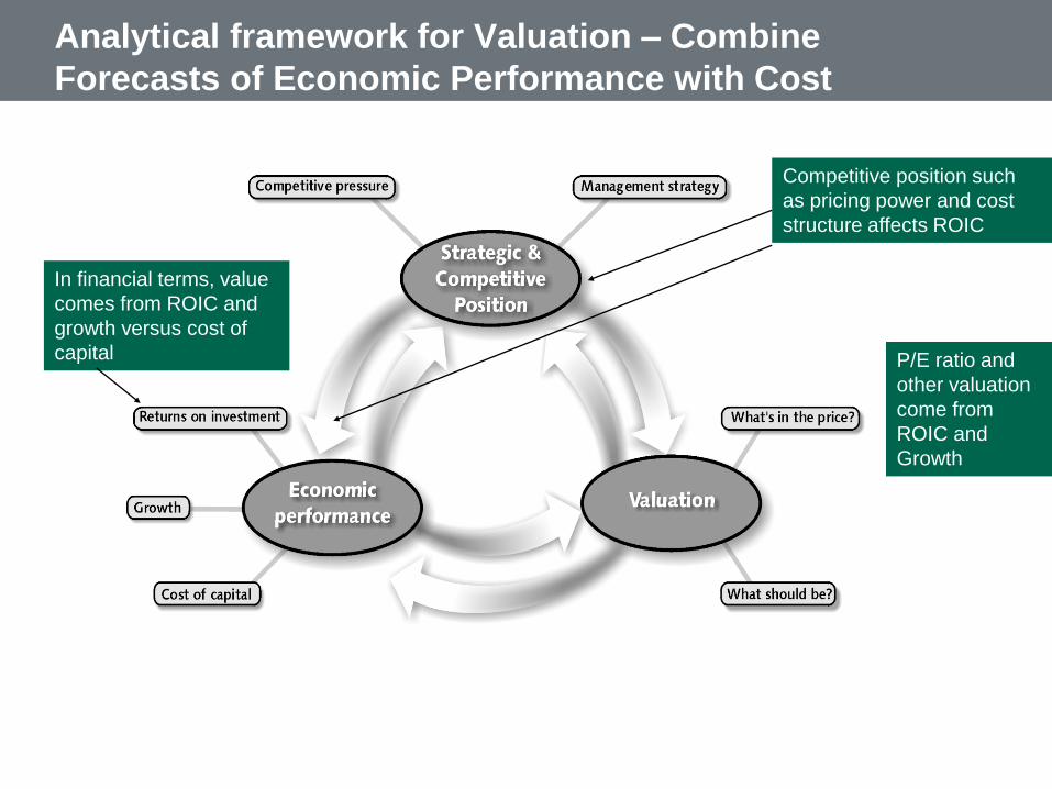
Analytical framework for Valuation – Combine
Forecasts of Economic Performance with Cost
of Capital
In financial terms, value
comes from ROIC and
growth versus cost of
capital
Competitive position such
as pricing power and cost
structure affects ROIC
P/E ratio and
other valuation
come from
ROIC and
Growth

Value Comes from Two Things
• What you think future cash flows will be
• How risky are those cash flows
We will deal with how to measure future cash flows and how to deal with
quantifying the risk of those cash flows
• Value comes from the ability to earn higher returns than the opportunity cost
of capital
• One of the few things we know is that there is a tradeoff between risk and
return.
Reference: Folder on Yield
Spreads

Valuation and Cash Flow
• Ultimately, value comes from cash flow in any model:
DCF – directly measure cash flow from explicit cash flow
and cash flow from selling after the explicit period
Multiples – The size of a multiple ultimately depends on cash
flow in formulas
FCF/(k-g) = Multiple
They still have implicit cost of capital and growth that
must be understood
Replacement Cost – cash from selling assets
• Growth rate in cash flow is a key issue in any of the models
Investors cannot buy a house with earnings or
use earnings for consumption or investment

Valuation Diagram
• Valuation using discounted cash flows requires forecasted cash
flows, application of a discount rate and measurement of
continuing value (also referred to as horizon value or terminal
value)
Cash Flow Cash Flow Cash Flow Cash Flow Continuing Value
Discount Rate is WACC
Enterprise Value
Net Debt
Equity Value
Reference: Private
Valuation; Valuation
Mistakes

Value Comes from Economic Profit and Growth
Capital Junkies
Power House
Capital Killers
Cash Cows
Growth +
Growth -
ROIC/WACC +
++ve -
Economic profit is
the difference
between profit and
opportunity cost
Once you have a
good thing, you
should grow
This implies that there
are three variables –
return, growth and
cost of capital that are
central to valuation
analysis
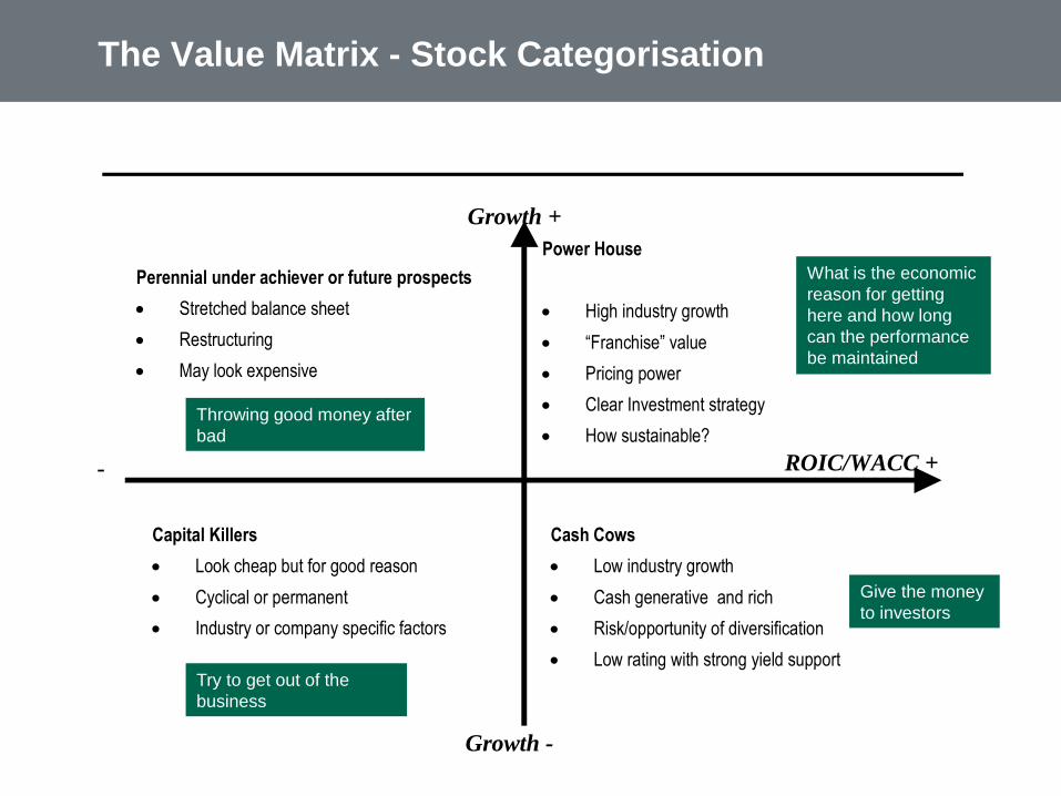
The Value Matrix - Stock Categorisation
Perennial under achiever or future prospects
Stretched balance sheet
Restructuring
May look expensive
Power House
High industry growth
“Franchise” value
Pricing power
Clear Investment strategy
How sustainable?
Capital Killers
Look cheap but for good reason
Cyclical or permanent
Industry or company specific factors
Cash Cows
Low industry growth
Cash generative and rich
Risk/opportunity of diversification
Low rating with strong yield support
Growth +
Growth -
ROIC/WACC +
++ve -
Throwing good money after
bad
Try to get out of the
business
What is the economic
reason for getting
here and how long
can the performance
be maintained
Give the money
to investors
ROIC Issues
• Issues with ROIC include
Will the ROIC move to WACC because of competitive pressures
Evidence suggests that ROIC can be sustained for long periods
Consider the underlying economic characteristics of the firm and the industry
What is the expected change in ROIC
When ROIC moves to sustainable level, then can move to terminal value
calculation
Examine the ROIC in models to determine if detailed assumptions are
leading to implausible results
Migration table

Reasonable Estimates of Growth
The short term
Based on best
estimate of likely
outcome
The medium term outlook
•Assessment of industry
outlook and company
position
• ROIC fades towards the
cost of capital
• Growth fades towards
GDP
The long run
• Long run
assumptions:
• ROIC = Cost of
capital
• Real growth = 0%
Much of valuation involves implicitly or explicitly
making growth estimates – High P/E comes from high
growthReference: Level and
persistence of growth rates
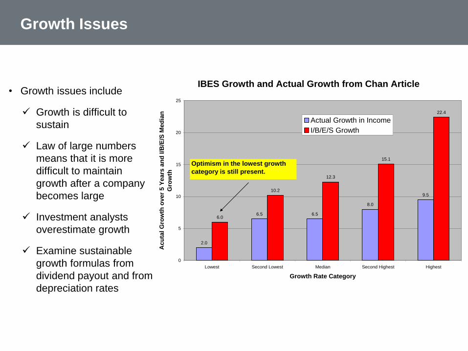
Growth Issues
• Growth issues include
Growth is difficult to
sustain
Law of large numbers
means that it is more
difficult to maintain
growth after a company
becomes large
Investment analysts
overestimate growth
Examine sustainable
growth formulas from
dividend payout and from
depreciation rates
IBES Growth and Actual Growth from Chan Article
2.0
6.5 6.5
8.0
9.5
6.0
10.2
12.3
15.1
22.4
0
5
10
15
20
25
Lowest Second Lowest Median Second Highest Highest
Growth Rate Category
Acu
tal G
row
th o
ver
5 Y
ea
rs a
nd
I/B
/E/S
Med
ian
Gro
wth
Actual Growth in Income
I/B/E/S Growth
Optimism in the lowest growth
category is still present.

Sustaining Growth and ROIC > WACC
• Mean Reversion of Long-term Growth
Competition tends to compress margins and growth
opportunities, and sub-par performance spurs corrective
actions.
With the passage of time, a firm’s performance tends to
converge to the industry norm.
Consideration should be given to whether the industry is in a
growth stage that will taper down with the passage of time or
whether its growth is likely to persist into the future.
Competition exerts downward pressure on product prices and
product innovations and changes in tastes tend to erode
competitive advantage. The typical firm will see the return
spread (ROIC-WACC) shrink over time.
A study by Chan,
Karceski, and
Lakonishok titled, “The
Level and Persistence
of Growth Rates,”
published in 2003.
According to this study,
analyst “growth
forecasts are overly
optimistic and add little
predictive power.”
Alternative Valuation Methods

Alternative Valuation Models
• There are many valuation techniques for assets and investments including:
Income Approach
Discounted Cash Flow
Venture Capital method
Risk Neutral Valuation
Sales Approach
Multiples (financial ratios) from Comparable Public Companies of from Transactions or from Theoretical Analysis
Liquidation Value
Cost Approach
Replacement Cost (New) and Reproduction Cost of similar assets
Other
Break-up Value
Options Pricing
• The different techniques should give consistent valuation answers

Example of Comparing Valuation under
Alternative Methods
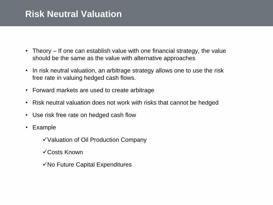
Risk Neutral Valuation
• Theory – If one can establish value with one financial strategy, the value
should be the same as the value with alternative approaches
• In risk neutral valuation, an arbitrage strategy allows one to use the risk
free rate in valuing hedged cash flows.
• Forward markets are used to create arbitrage
• Risk neutral valuation does not work with risks that cannot be hedged
• Use risk free rate on hedged cash flow
• Example
Valuation of Oil Production Company
Costs Known
No Future Capital Expenditures
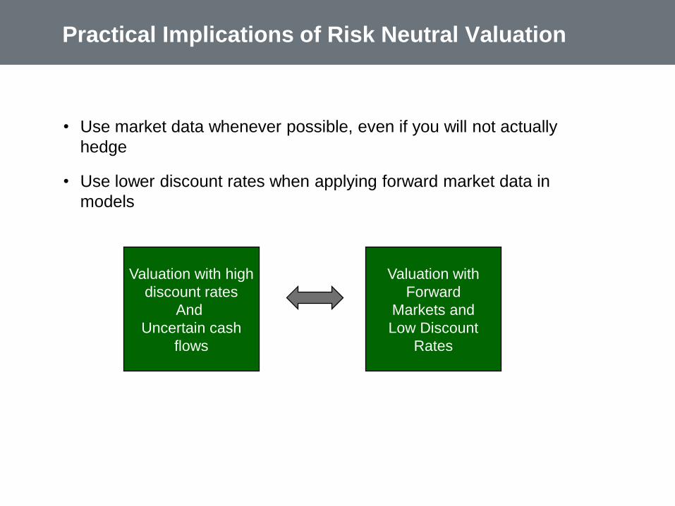
Practical Implications of Risk Neutral Valuation
• Use market data whenever possible, even if you will not actually
hedge
• Use lower discount rates when applying forward market data in
models
Valuation with high
discount rates
And
Uncertain cash
flows
Valuation with
Forward
Markets and
Low Discount
Rates
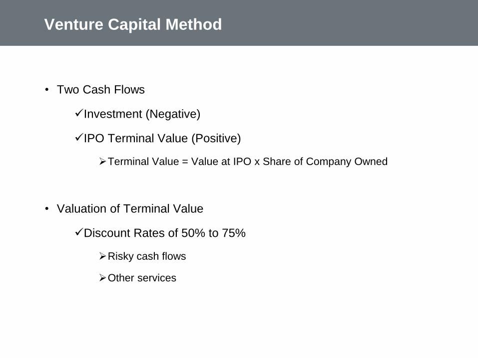
Venture Capital Method
• Two Cash Flows
Investment (Negative)
IPO Terminal Value (Positive)
Terminal Value = Value at IPO x Share of Company Owned
• Valuation of Terminal Value
Discount Rates of 50% to 75%
Risky cash flows
Other services

Valuation Diagram – Venture Capital
• Valuation in venture capital focuses on the value when you will
get out, the discount rates and how much of the company you will
own when you exit.
Cash Flow Cash Flow Cash Flow Cash Flow Continuing Value
Discount Rates
Enterprise Value
Net Debt
Equity Value
Evaluate how much of the
equity value that you own
•In the extreme, if you
have given away half of
your company away,
and the cash flow is the
same before and after
your give away, then the
amount you would pay
for the share must
account for how much
you will give away.
Venture Capital Method
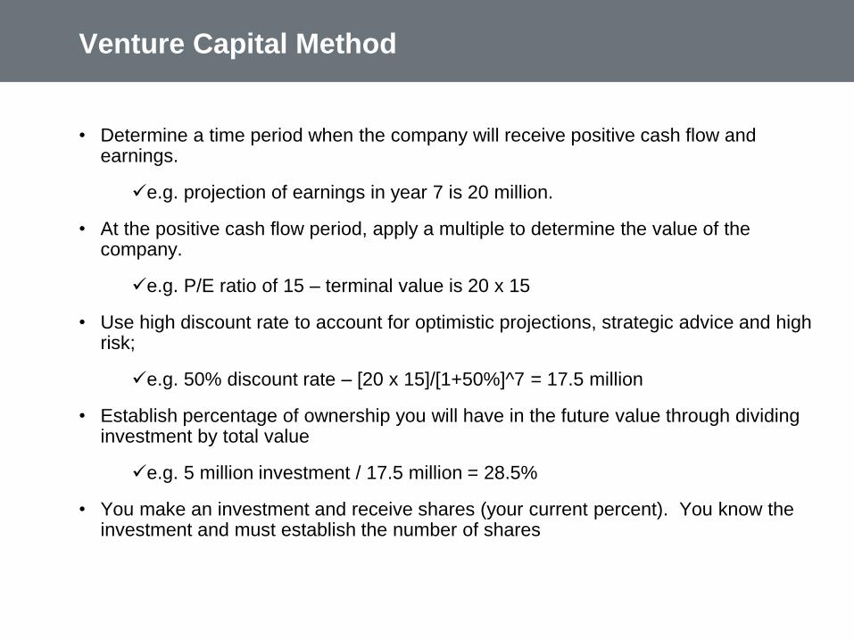
• Determine a time period when the company will receive positive cash flow and earnings.
e.g. projection of earnings in year 7 is 20 million.
• At the positive cash flow period, apply a multiple to determine the value of the company.
e.g. P/E ratio of 15 – terminal value is 20 x 15
• Use high discount rate to account for optimistic projections, strategic advice and high risk;
e.g. 50% discount rate – [20 x 15]/[1+50%]^7 = 17.5 million
• Establish percentage of ownership you will have in the future value through dividing investment by total value
e.g. 5 million investment / 17.5 million = 28.5%
• You make an investment and receive shares (your current percent). You know the investment and must establish the number of shares

Venture Capital Method Continued
• In the venture capital method, there are only two cash flows
The investment
The value when the company is sold
• The value received when the company is sold depends on the percentage of the
company that is owned. If there is dilution in ownership, the value is less.
• Therefore, an adjustment must be made for dilution and the percent of the company
retained. See the Cost of Capital folder for and example
e.g. Share value without dilution = 17.5/700,000 = 25 per share
If an additional 30% of shares is floated, the value per share must be
increased by 30% to maintain the value.
Value per share = 17.5/((500,000+VC shares) x 1.3)
VC Shares: (25 x 1.3)/17.5-500,000 = 343,373
Replacement Cost
• First a couple of points regarding replacement cost theory
In theory, one can replace the assets of a company without investing
in the company. If you are valuing a company, you may think about
creating the company yourself.
If you replaced a company and really measured the replacement
cost, the value of the company may be more than replacement cost
because the company manages the assets better than you could.
By replacing the assets and entering the business, you would
receive cash flows. You can reconcile the replacement cost with the
discounted cash flow approach
Measuring Replacement Cost
• Replacement cost includes:
Value of hard assets
Value of patents and other intangibles
Cost of recruiting and training management
• Analysis
Begin with balance sheet categories, account for the age of the plant
Add: cost of hiring and training management
• If the company is generating more cash flow than that would be produced
from replacement cost, the management may be more productive than
others in managing costs or be able to realize higher prices through
differentiation of products.
• The ratio of market value to replacement cost is a theoretical ratio that
measures the value of management contribution

Replacement Value and Tobin’s Q
• Recall Tobin’s Q as:
Q = Enterprise Value / Replacement Cost
• Buy assets and talent etc and should receive the ROIC. Earn
industry average ROIC.
If the ROIC > industry average, then Q > 1.
If the ROIC < industry average, then Q < 1
Real Options and Problems with DCF
• The DCF model has many conceptual flaws, the most significant
of which is assuming that cash flows are normally distributed
around the mean or base case level.
• For many investments, the cash flows are skewed:
When an asset is to be retired, there is more upside than downside
because the asset will continue to operate when times are good, but
it will be scrapped when times are bad.
An investment decision often involves the possibility to expand in the
future. When the expansion decision is made, it will only occur when
the economics are good.
During the period of constructing an asset, it is possible to cancel
the construction expenditures and limit the downside if it becomes
clear that the project will not be economic.
Real Options and DCF Problems - Continued
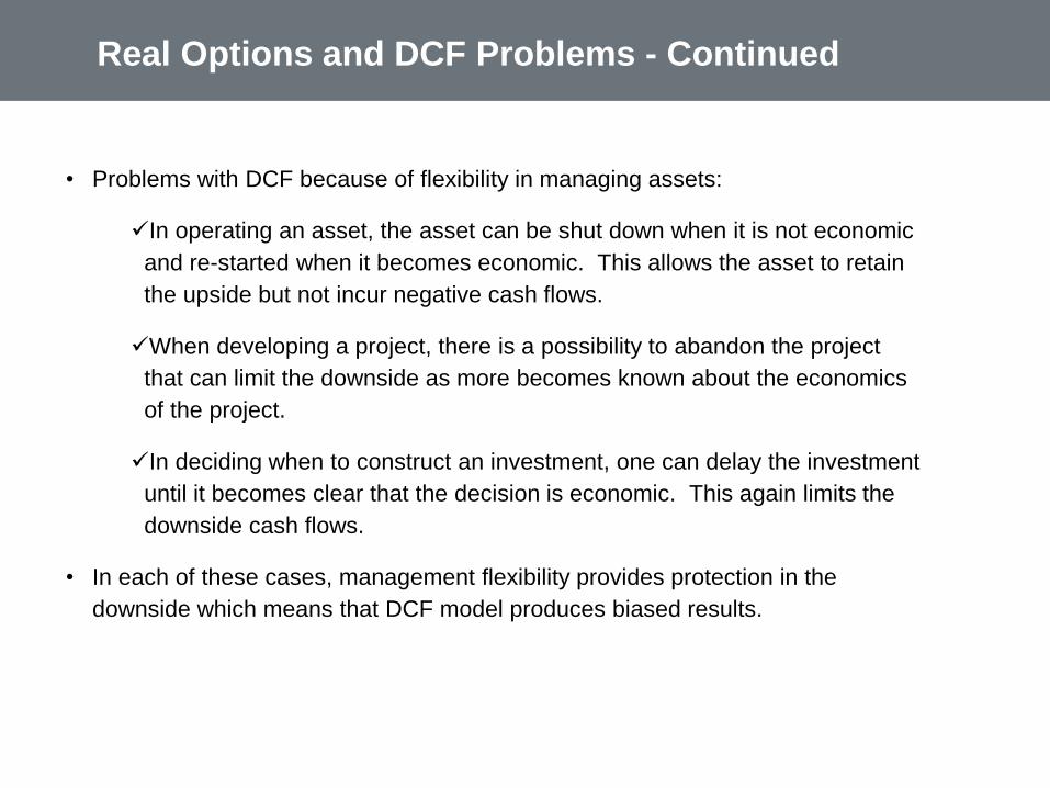
• Problems with DCF because of flexibility in managing assets:
In operating an asset, the asset can be shut down when it is not economic
and re-started when it becomes economic. This allows the asset to retain
the upside but not incur negative cash flows.
When developing a project, there is a possibility to abandon the project
that can limit the downside as more becomes known about the economics
of the project.
In deciding when to construct an investment, one can delay the investment
until it becomes clear that the decision is economic. This again limits the
downside cash flows.
• In each of these cases, management flexibility provides protection in the
downside which means that DCF model produces biased results.

Fundamental Valuation
• What was behind the bull market of 1980-1999
EPS rose from 15 to 56
Nominal growth of 6.9% -- about the growth in the real economy (the
real GDP)
Keeping P/E constant would have large share price increase
Long-term interest rates fell – lower cost of capital increases the P/E
ratio
• Real Market
Value by ROIC versus growth
Select strategies that lead to economic profit
Market value from expected performance

Three Primary Methods Discussed in Remainder of
Slides
• Market Multiples
• Discounted Free Cash Flow
• Discounted Earnings and Dividends
• Warning: No method is perfect or completely precise
• Use industry expertise and judgement in assessing discount rates
and multiples
• Different valuation methods should yield similar results
• Bangor Hydro Case

Discounting Basics

Bt = It +1 + It +2 + It +3 + ... + It +n + F
(1+r)1 (1+r)2 (1+r)3 (1+r)n (1+r)n
Debt (Bond) Valuation
• Bt is the value of the bond at time t
• Discounting in the NPV formula assumes END of period
• It +n is the interest payment in period t+n
• F is the principal payment (usually the debt’s face value)
• r is the interest rate (yield to maturity)
Case exercise to illustrate
the effect of discounting
(credit spread) on the value
of a bond

Risk Free Discounting
• If the world would involve discounting cash flows at the risk free rate,
life would be easy and boring
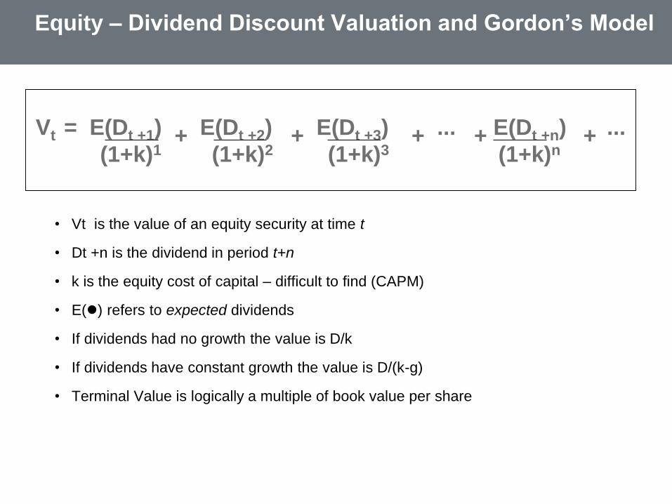
Vt = E(Dt +1) + E(Dt +2) + E(Dt +3) + ... + E(Dt +n) + ...
(1+k)1 (1+k)2 (1+k)3 (1+k)n
Equity – Dividend Discount Valuation and Gordon’s Model
• Vt is the value of an equity security at time t
• Dt +n is the dividend in period t+n
• k is the equity cost of capital – difficult to find (CAPM)
• E() refers to expected dividends
• If dividends had no growth the value is D/k
• If dividends have constant growth the value is D/(k-g)
• Terminal Value is logically a multiple of book value per share
Example of Capitalization Rates
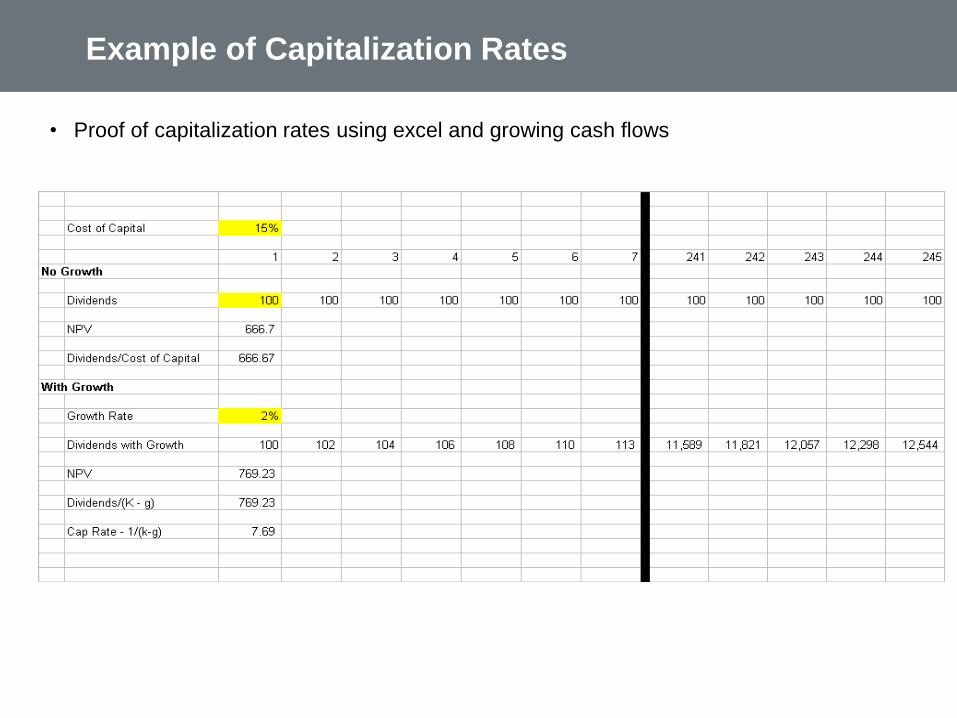
• Proof of capitalization rates using excel and growing cash flows
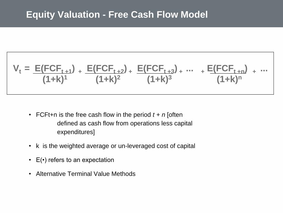
Vt = E(FCFt +1) + E(FCFt +2) + E(FCFt +3) + ... + E(FCFt +n) + ...
(1+k)1 (1+k)2 (1+k)3 (1+k)n
• FCFt+n is the free cash flow in the period t + n [often
defined as cash flow from operations less capital
expenditures]
• k is the weighted average or un-leveraged cost of capital
• E(•) refers to an expectation
• Alternative Terminal Value Methods
Equity Valuation - Free Cash Flow Model

Practical Discounting Issues in Excel
• NPV formula assumes end of period cash flow
• Growth rate is ROE x Retention rate
• If you are selling the stock at the end of the last period and doing
a long-term analysis, you must use the next period EBITDA or the
next period cash flow.
• If there is growth in a model, you should use the add one year of
growth to the last period in making the calculation
• To use mid-year of specific discounting use the IRR or XIRR or
sumproduct

Valuation and Sustainable Growth
• Value depends on the growth in cash flow. Growth can be estimated
using alternative formulas:
Growth in EPS = ROE x (1 – Dividend Payout Ratio)
Growth in Investment = ROIC x (1-Reinvestment Rate)
Growth = (1+growth in units) x (1+inflation) – 1
• When evaluating NOPLAT rather than earnings, a similar concept can be
used for sustainable growth.
Growth = (Capital Expenditures/Depreciation – 1) x Depreciation
Rate
• Unrealistic to assume growth in units above the growth in the economy on
an ongoing basis.

Valuation Using Multiples
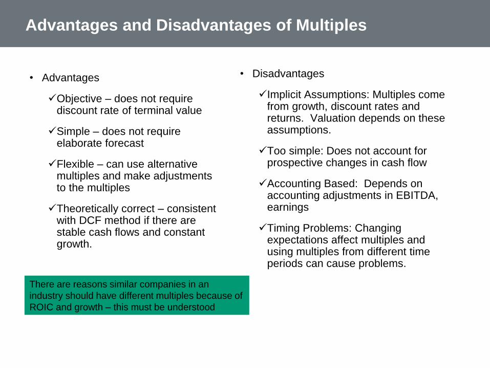
Advantages and Disadvantages of Multiples
• Advantages
Objective – does not require discount rate of terminal value
Simple – does not require elaborate forecast
Flexible – can use alternative multiples and make adjustments to the multiples
Theoretically correct – consistent with DCF method if there are stable cash flows and constant growth.
• Disadvantages
Implicit Assumptions: Multiples come from growth, discount rates and returns. Valuation depends on these assumptions.
Too simple: Does not account for prospective changes in cash flow
Accounting Based: Depends on accounting adjustments in EBITDA, earnings
Timing Problems: Changing expectations affect multiples and using multiples from different time periods can cause problems.
There are reasons similar companies in an
industry should have different multiples because of
ROIC and growth – this must be understood
Multiples - Summary
• Useful sanity check for valuation from other methods
• Use multiples to avoid subjective forecasts
• Among other things, well done multiple that accounts for
Accounting differences
Inflation effects
Cyclicality
• Use appropriate comparable samples
• Use forward P/E rather than trailing
• Comprehensive analysis of multiples is similar to forecast
• Use forecasts to explain why multiples are different for a specific company

Mechanics of Multiples
• Find market multiple from comparable companies
Rarely are there truly comparable companies
Understand economics that drive multiples (growth rate, cost of capital and return)
• P/E Ratio (forward versus trailing)
Value/Share = P/E x Projected EPS
P/E trailing and forward multiples
• Market to Book
Value/Share = Market to Book Ratio x Book Value/Share
• EV/EBITDA
Value/Share = (EV/EBITDA x EBITDA – Debt) divided by shares
• P/E and M/B use equity cash flow; EV/EBITDA uses free cash flow
In the long-term P/E ratios tend to
revert to a mean of 15.0

Valuation from Multiples
• Financial Multiples
P/E Ratio
EV/EBITDA
Price/Book
• Industry Specific
Value/Oil Reserve
Value/Subscriber
Value/Square Foot
• Issues
Where to find the multiple data – public companies
What income or cash flow base to use
15-20% Discount for lack of marketability

Which Multiple to Use
• Valuation from multiples uses information from other companies
• It is relevant when the company is already in a steady state situation and there is
no reason to expect that you can improve estimates of EBITDA or Earnings
• One of the challenges is to understand which multiple works in which situation:
Consumer products
EV/EBITDA may be best
Intangible assets make book value inappropriate
Different leverage makes P/E difficult
Banks/Insurance
Market/Book may be best
Not many intangible assets, so book value is meaningful
Book value is the value of loans which is adjusted with loan loss provisions
Cost of capital and financing is very important because of the cost of
deposits

Multiples in M&A
• Public company comparison
• Precedent Transactions
• Issues
Where to find the data
Finding comparable companies
Timing (changes in multiples with market moves)
What data to apply data to (e.g. next year’s earnings)
What do ratios really mean (e.g. P/E Ratio)
Adjustments for liquidity and control premium

Comparable companies analysis data in a
Chinese Banking Merger
Statistics on Comparable Companies Chinese Agricultural Bank
Multiple of Market Value Per Share Implied Per Share Equity Value
LTM High Low Mean Median ActualValues 3,000,000 High Low Mean Median
Total Assets 0.359x 0.093x 0.162x 0.152x $337,932,000 112.64 40.44 10.48 18.25 17.12 Tangible Book
Value* 2.490x 1.155x 1.688x 1.719x $35,545,737 11.85 25.28 13.25 18.05 18.33 LTM EPS 85.000x 10.131x 17.181x 13.085x $3,545,737 1.182 100.46 11.97 20.31 15.47
2002 Est EPS 28.333x 9.350x 13.037x 12.195x $5,172,415 1.724 48.85 16.12 22.48 21.03 2003 Est EPS 14.856x 8.611x 11.288x 11.255x $5,883,841 1.961 29.14 16.89 22.14 22.07
*Normalized book value, assuming 8 percent equity as 'normal.' Source: SNL Securities, 2002 (Pricing as of 3/25/2002). Summary of 21 comparable banking companies with similar assets, capital and profitability characteristics.
Note the ratios used to value banks are equity based – the Market
value to Book Value and the P/E ratio related to various earnings
measures

Comparison with all Acquisitions Since 2001
All Asian Banking Acquisitions with a total deal value over $200m
SOV-Waypoint Deals in 2004 Deals since 2003 Deals since 2002 Deals since 2001
# of Deals 1 7 16 20 28
Median 238.5 256.1 238.7 238.7
Mean 241.0 249.6 240.8 244.6
Median 304.7 299.2 290.4 299.2
Mean 319.3 309.6 301.4 307.3
Median 20.7 20.4 20.3 20.3
Mean 20.9 20.3 19.9 20.2
Median 29.9 30.4 30.1 30.2
Mean 31.4 32.8 32.1 31.4
238.5
251.8
22.0
32.1
Price/Book
Price/Tangible Book
Price/LTM Earnings
Price/Deposits

Adjustments to Multiples
• Process
Find multiples from similar public companies
Adjust multiples for
Liquidity
Size
Control premium
Developing country discount
Apply adjusted multiples to book value, earnings, and EBITDA
• There is often more money in dispute in determining the discounts and premiums in a
business valuation than in arriving at the pre-discount valuation itself. Discounts and
premiums affect not only the value of the company, but also play a crucial role in
determining the risk involved, control issues, marketability, contingent liability, and a
host of other factors.
• If the entity were closely held with no (or little) active market for the
shares or interest in the company, then a non-marketability discount
would be subtracted from the value.
• Non-marketabiliy Discounts – ranges from 10% to 30%
• …represents the reduction in value from a marketable interest level
of value to compensate an investor for illiquidity of the security, all
else equal.
• The size of the discount varies base on:
relative liquidity (such as the size of the shareholder base);
the dividend yield, expected growth in value and holding period;
and firm specific issues such as imminent or pending initial public
offering (IPO) of stock to be freely traded on a public market.
Adjustments to Multiples – Marketability and
Liquidity Discount
Studies of Liquidity Discount
• Private and public transactions
Attempt to compute EV/EBITDA in public and private transactions
Adjust so that the transactions are comparable
Compute the ratio in pubic and private transactions
Discount of 20 to 28 percent for US firms
Discount of 44 to 54 percent for non-US firms
• Other studies
Value in IPO versus value of private trades before IPO
High liquidity in 40-50% range, but selection bias
Theory involves control by public board
P/E Analysis – Use of P/E Ratio in Valuation
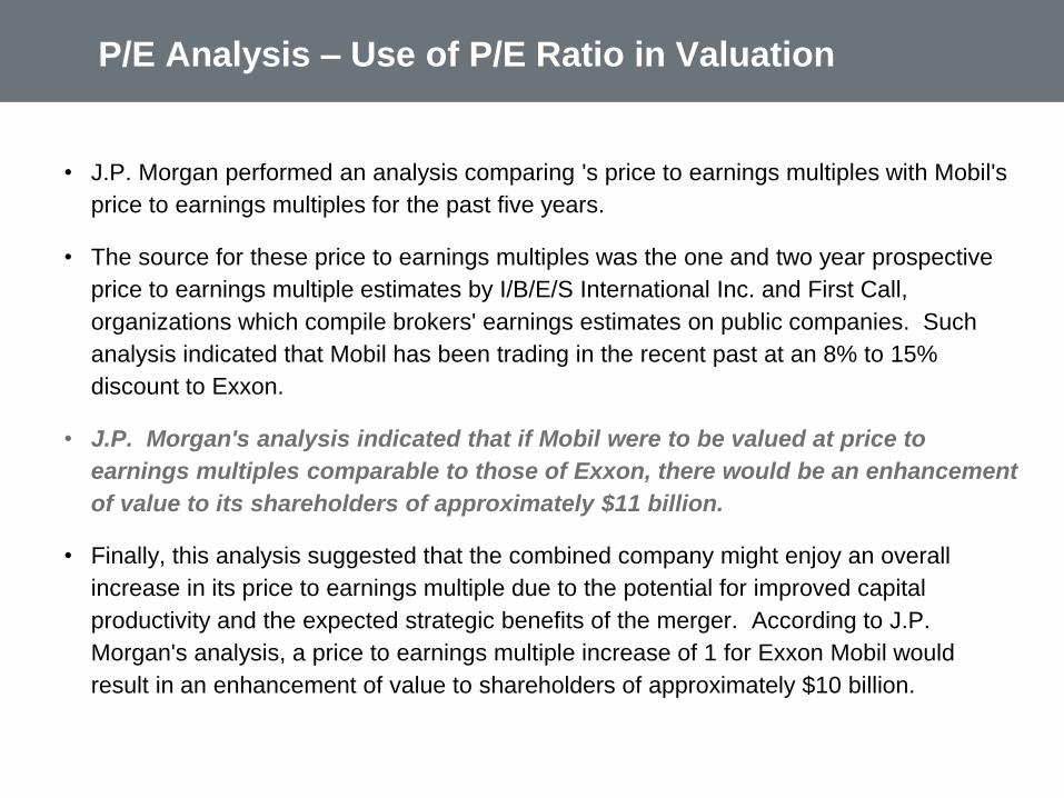
• J.P. Morgan performed an analysis comparing 's price to earnings multiples with Mobil's
price to earnings multiples for the past five years.
• The source for these price to earnings multiples was the one and two year prospective
price to earnings multiple estimates by I/B/E/S International Inc. and First Call,
organizations which compile brokers' earnings estimates on public companies. Such
analysis indicated that Mobil has been trading in the recent past at an 8% to 15%
discount to Exxon.
• J.P. Morgan's analysis indicated that if Mobil were to be valued at price to
earnings multiples comparable to those of Exxon, there would be an enhancement
of value to its shareholders of approximately $11 billion.
• Finally, this analysis suggested that the combined company might enjoy an overall
increase in its price to earnings multiple due to the potential for improved capital
productivity and the expected strategic benefits of the merger. According to J.P.
Morgan's analysis, a price to earnings multiple increase of 1 for Exxon Mobil would
result in an enhancement of value to shareholders of approximately $10 billion.

Price Earnings Ratio
• The price earnings ratio is obviously very important in stock evaluation.
Therefore, I describe some background related to the ratio and some theory
with regards to the P/E ratio. Subjects related to the P/E ratio include:
Dividend growth Model
Theory of price earnings ratio and growth
P/E ratio and the EV/EBITDA ratio
The PE ratio depends more on accounting
The PE is affected by leverage
The EV/EBITDA ignores depreciation and capital expenditure
Case exercise on P/E and EV/EBITDA

P/E Ratio versus EV/EBITDA
• Use the EV/EBITDA when the funding does not make much difference in
valuation
Many companies in an industry with different levels of gearing and
companies do not attempt to maximize leverage
Very high levels of gearing and wildly fluctuating earnings
When the earnings are affected by accounting policy and account
adjustments
• Use the P/E ratio when cost of funding clearly affects valuation and/or
when the level of gearing is stable and similar for different companies
Debt capacity can provide essential information on valuation
EBITDA does not account for taxes, capital expenditures to replace
existing assets, depreciation and other accounting factors that can
affect value.

P/E Ratio
• If you use the P/E ratio for valuation, the ratio implies that only this year or
last years earnings matter
• Cash matters to investors in the end, not earnings (different lifetime of
earnings)
• When earnings reflect cash flow, P/E is reasonable for valuation
• High P/E causes treadmill and does not necessary imply that companies
are performing well
• Earnings can be managed and manipulated
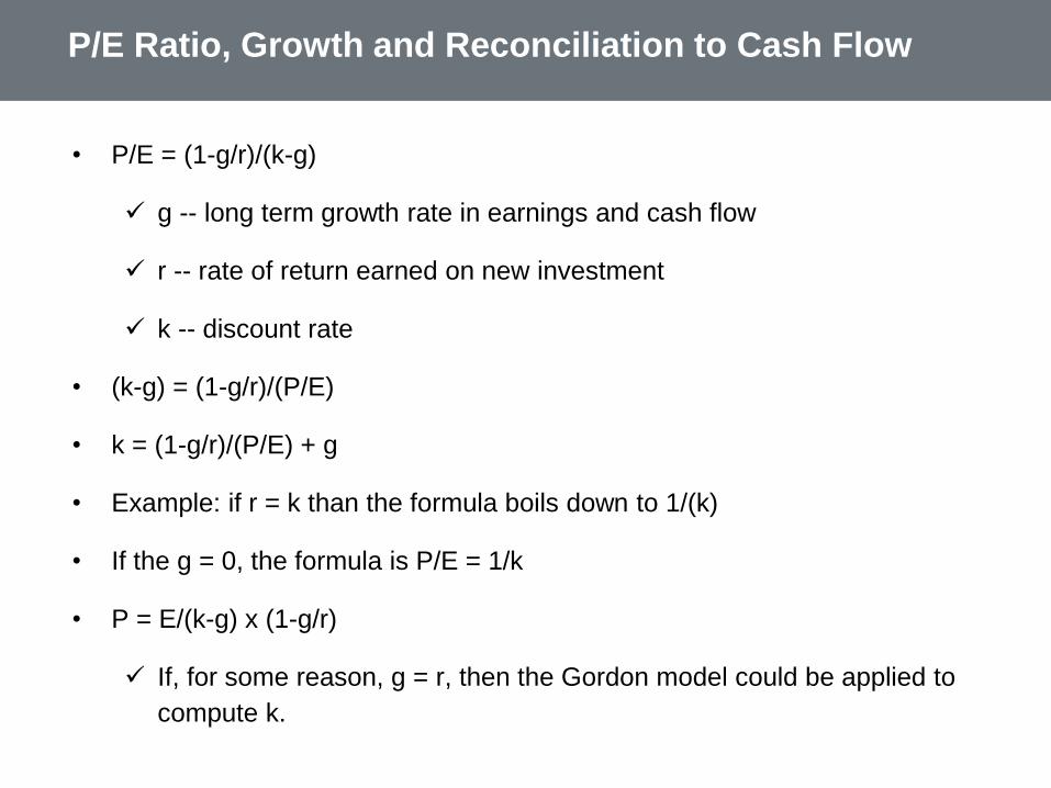
P/E Ratio, Growth and Reconciliation to Cash Flow
• P/E = (1-g/r)/(k-g)
g -- long term growth rate in earnings and cash flow
r -- rate of return earned on new investment
k -- discount rate
• (k-g) = (1-g/r)/(P/E)
• k = (1-g/r)/(P/E) + g
• Example: if r = k than the formula boils down to 1/(k)
• If the g = 0, the formula is P/E = 1/k
• P = E/(k-g) x (1-g/r)
If, for some reason, g = r, then the Gordon model could be applied to
compute k.

PE Ratio Formula when k = r – There is no economic
profit on new investments
• P/E = (1-g/r)/(k-g)
If k = r
P/E = (1-g/k)/(k-g)
P/E = (k/k-g/k)/(k-g)
P/E = ((k-g)/k)/(k-g)
P/E = 1/k
• PEG Ratio P/E divided by g
If the g and the r were the same, the ratio would be a benchmark
Should consider the r and the k

Use of P/E Ratio Formula to Compute the Required
Return on Equity Capital
• It will become apparent later that one cannot get away from estimating the
cost of equity capital and the CAPM technique is inadequate from a theoretical
and a practical standpoint.
• The following example illustrates how the formula can be used in practice:
k = (1-g/r)/(P/E) + g
•
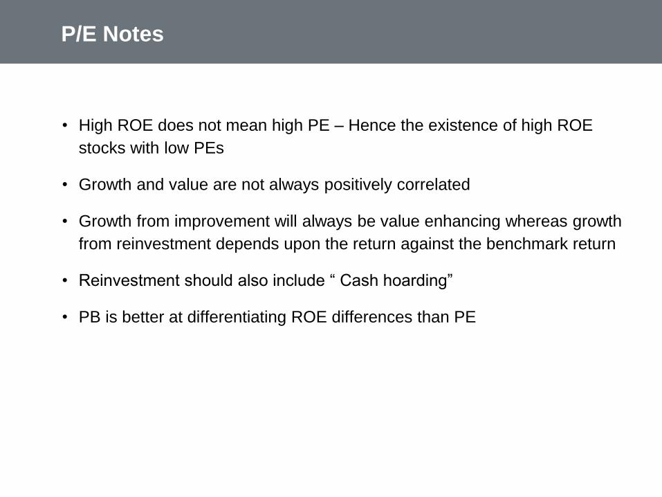
P/E Notes
• High ROE does not mean high PE – Hence the existence of high ROE
stocks with low PEs
• Growth and value are not always positively correlated
• Growth from improvement will always be value enhancing whereas growth
from reinvestment depends upon the return against the benchmark return
• Reinvestment should also include “ Cash hoarding”
• PB is better at differentiating ROE differences than PE
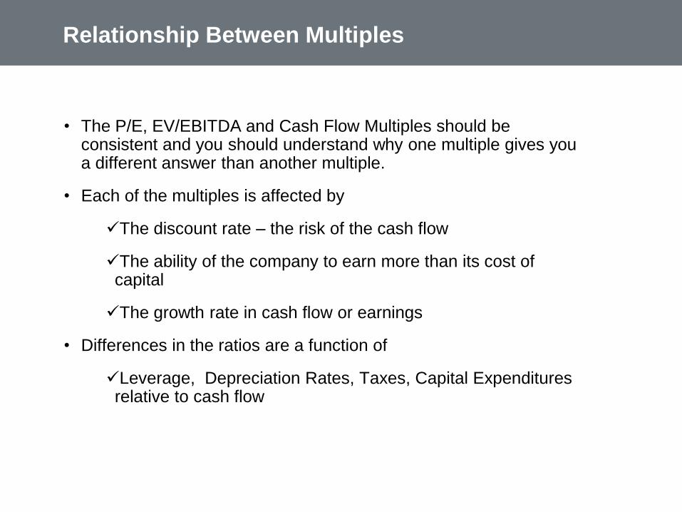
Relationship Between Multiples
• The P/E, EV/EBITDA and Cash Flow Multiples should be consistent and you should understand why one multiple gives you a different answer than another multiple.
• Each of the multiples is affected by
The discount rate – the risk of the cash flow
The ability of the company to earn more than its cost of capital
The growth rate in cash flow or earnings
• Differences in the ratios are a function of
Leverage, Depreciation Rates, Taxes, Capital Expenditures relative to cash flow

Relationship Between Multiples
• Enterprise Value = NOPLAT x (1-g/ROIC)/(WACC – g)
• NOPLAT = Investment x ROIC
• NOPLAT = EBIT x (1-t)
• EBITDA = EBIT + Depreciation
EV/EBITDA
• EBT = EBIT – Interest
• NI = EBT x (1-t)
NI/Market Cap
• Market Cap = EV – Debt
MB = Market Cap/Equity
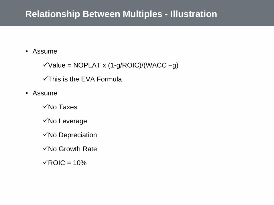
Relationship Between Multiples - Illustration
• Assume
Value = NOPLAT x (1-g/ROIC)/(WACC –g)
This is the EVA Formula
• Assume
No Taxes
No Leverage
No Depreciation
No Growth Rate
ROIC = 10%
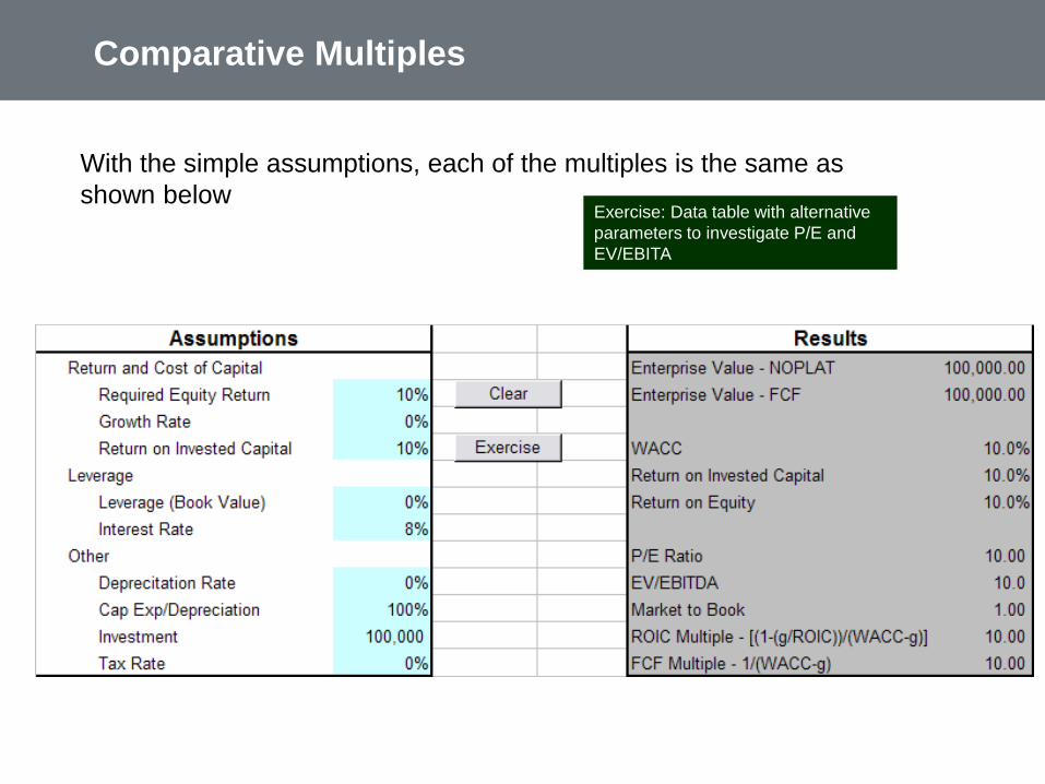
Comparative Multiples
With the simple assumptions, each of the multiples is the same as
shown belowExercise: Data table with alternative
parameters to investigate P/E and
EV/EBITA
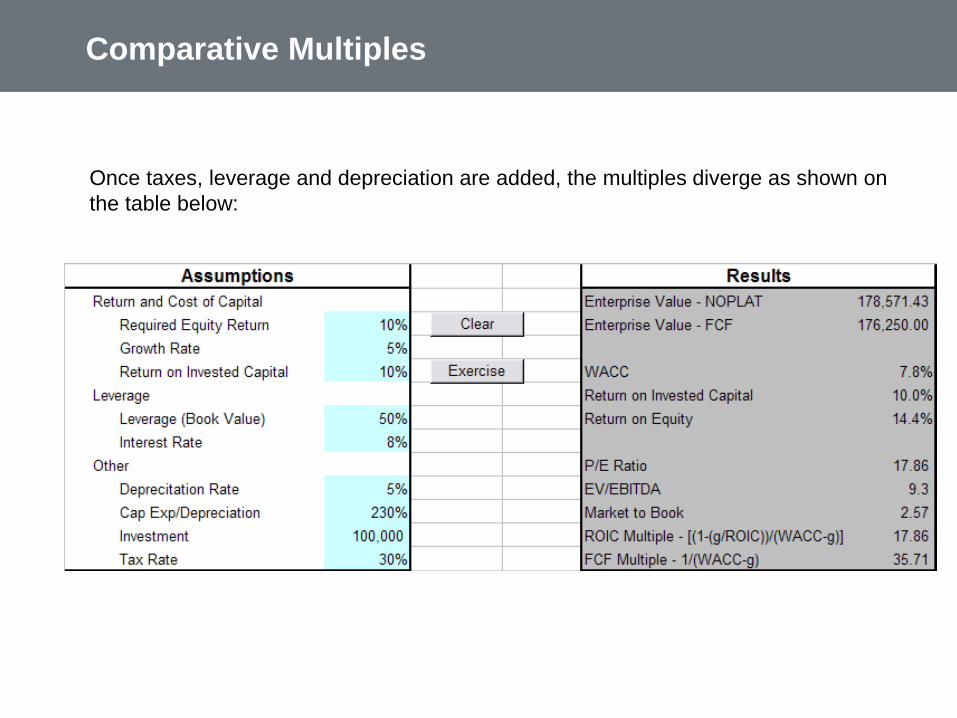
Comparative Multiples
Once taxes, leverage and depreciation are added, the multiples diverge as shown on
the table below:
Problems in Applying Multiples
• If you assume that the company has been growing at a high rate
and apply the P/E ratio will be overstated in valuation.
• When comparing companies, the operating leverage and financial
risks should be similar and there should be an understanding of
why P/E ratios are different.
• In applying multiples for comparable transactions, if synergy
values are added, there is double counting
• If industry has cycles, must be careful in application

Market and sector PE ratios – The danger of averages
This chart illustrates issues associate with computing averages. In practice,
the number of comparable firms is small and choosing the median is
advisable.

Valuation From Discounted Free Cash Flow

Advantages and Disadvantages of DCF
• Advantages
Theoretically Valid – value comes
from free cash flow and assessing
risk of the free cash flow.
Operating and Financial Values –
explicitly separates value from
operating the company with value
of financial obligations and value
from cash
Sensitivity – forces an
understanding of key drivers and
allows sensitivity and scenario
analysis
• Disadvantages
Assumptions: Requires WACC
assumptions and residual value
assumptions. There are major
problems with WACC estimation.
Forecasting Problems: Complex
forecasting models can easily be
manipulated
Growth: The residual value depends
on growth rates which can easily
distort value
Real Options: Discussed above

Discounted Flow
• Use the discounted cash flow when you know something more
about the company that can be obtained with a forecast
• Any cash flow forecast involves:
Value =
Cash flow during explicit forecast period +
Present of cash flow after explicit forecast period
• The second item generally involves some kind of growth
projection.
• Value of Equity = Value of Enterprise – Value of Net Debt
Discounted Cash Flow
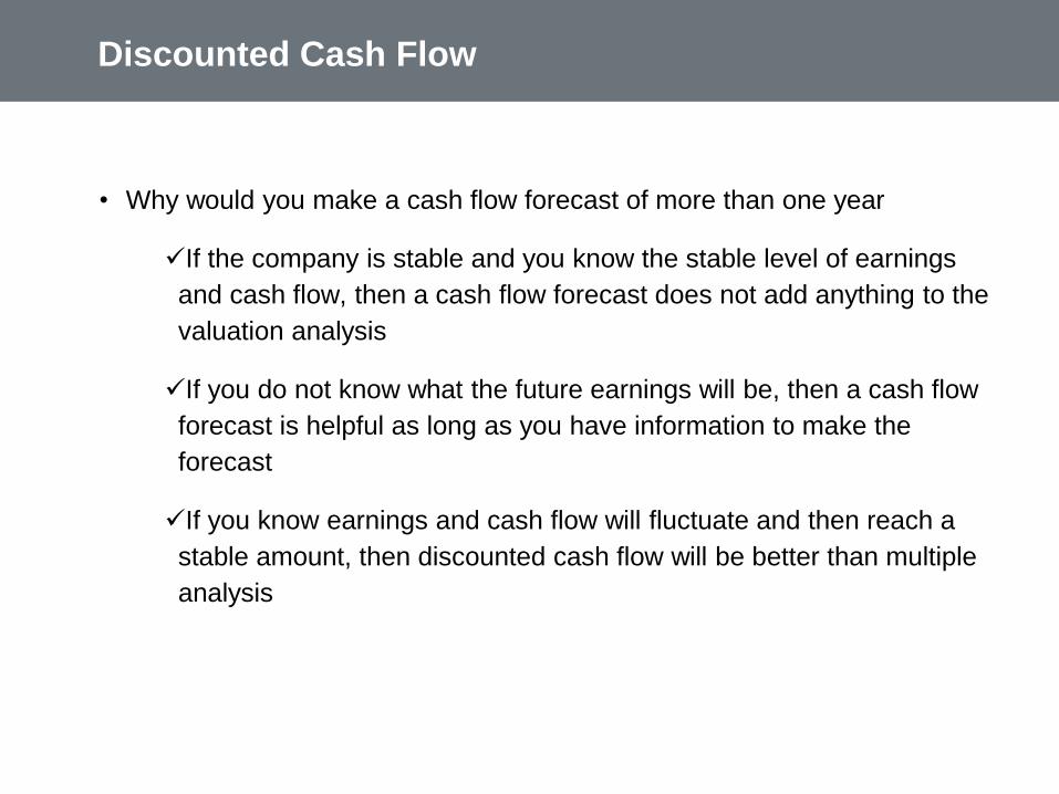
• Why would you make a cash flow forecast of more than one year
If the company is stable and you know the stable level of earnings
and cash flow, then a cash flow forecast does not add anything to the
valuation analysis
If you do not know what the future earnings will be, then a cash flow
forecast is helpful as long as you have information to make the
forecast
If you know earnings and cash flow will fluctuate and then reach a
stable amount, then discounted cash flow will be better than multiple
analysis
Step by Step Valuation with Free Cash Flow
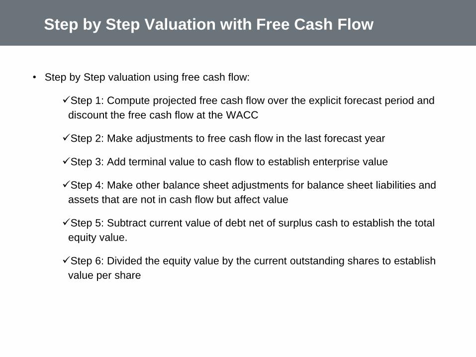
• Step by Step valuation using free cash flow:
Step 1: Compute projected free cash flow over the explicit forecast period and
discount the free cash flow at the WACC
Step 2: Make adjustments to free cash flow in the last forecast year
Step 3: Add terminal value to cash flow to establish enterprise value
Step 4: Make other balance sheet adjustments for balance sheet liabilities and
assets that are not in cash flow but affect value
Step 5: Subtract current value of debt net of surplus cash to establish the total
equity value.
Step 6: Divided the equity value by the current outstanding shares to establish
value per share
Assets and Liabilities that Escape DCF Valuation
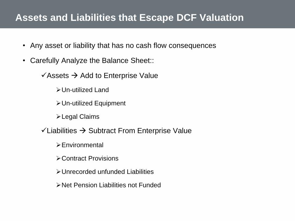
• Any asset or liability that has no cash flow consequences
• Carefully Analyze the Balance Sheet::
Assets Add to Enterprise Value
Un-utilized Land
Un-utilized Equipment
Legal Claims
Liabilities Subtract From Enterprise Value
Environmental
Contract Provisions
Unrecorded unfunded Liabilities
Net Pension Liabilities not Funded
Double Counting of Assets and Obligations
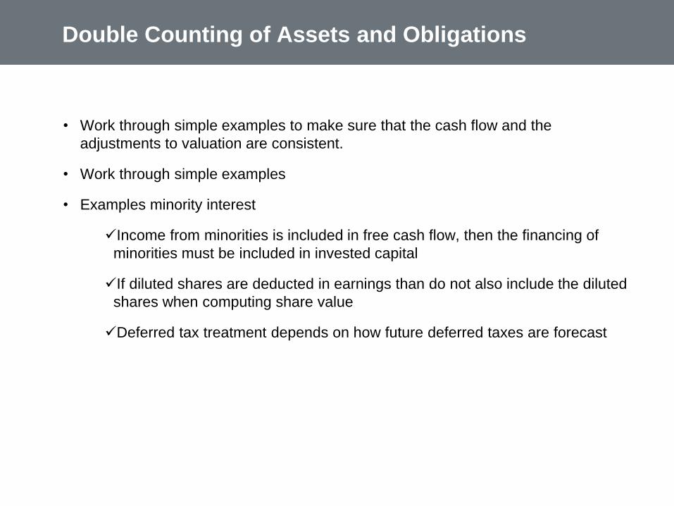
• Work through simple examples to make sure that the cash flow and the
adjustments to valuation are consistent.
• Work through simple examples
• Examples minority interest
Income from minorities is included in free cash flow, then the financing of
minorities must be included in invested capital
If diluted shares are deducted in earnings than do not also include the diluted
shares when computing share value
Deferred tax treatment depends on how future deferred taxes are forecast

DCF Valuation – Length of Forecast
• Short-run
Forecast all financial statement items
Gross-margin, selling expenses, Etc.
• Further out
Individual line items more difficult
Focus on key drivers
Operating margin, tax rate, capital efficiency
• Continuing Value
When ROIC and growth stabalise
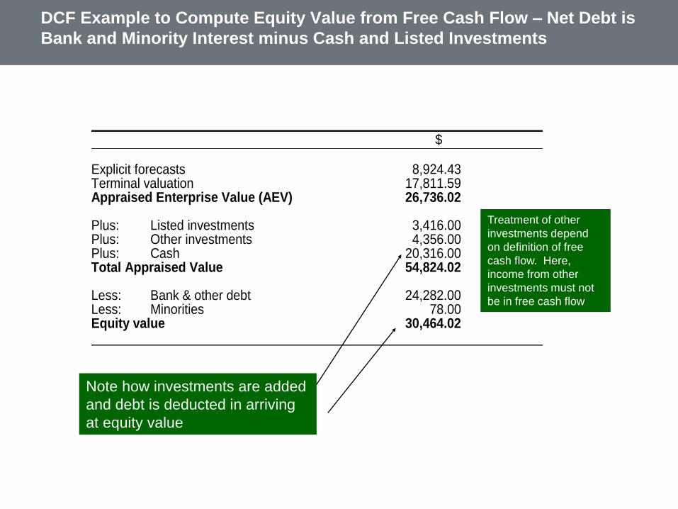
$ Explicit forecasts 8,924.43 Terminal valuation 17,811.59 Appraised Enterprise Value (AEV) 26,736.02 Plus: Listed investments 3,416.00 Plus: Other investments 4,356.00 Plus: Cash 20,316.00 Total Appraised Value 54,824.02 Less: Bank & other debt 24,282.00 Less: Minorities 78.00 Equity value 30,464.02
DCF Example to Compute Equity Value from Free Cash Flow – Net Debt is
Bank and Minority Interest minus Cash and Listed Investments
Note how investments are added
and debt is deducted in arriving
at equity value
Treatment of other
investments depend
on definition of free
cash flow. Here,
income from other
investments must not
be in free cash flow
Continuing Value
Estimating Continuing Value
• Continuing value is important aspect of valuation
• In actual valuations compiled by MONITOR, the terminal value is – 56% to
125% of valuation
• High terminal values are reasonable if cash flow in early years is offset by
outflows for capital spending that should generate higher cash flows in later
years
The terminal value should reflect cash flow and earnings that is at the middle
of the business cycle, or in the case of commodities, where prices reflect
long-run marginal production cost, or in the case of high growth companies,
when the market is saturated

• Terminal or continuing value is analogous to dividends and capital gains.
Free cash flow is dividends, residual value is capital gain.
• A few methods of computing residual value include:
Perpetuity
EBITDA Multiple
P/E Ratio
Market to Book Ratio
Replacement Cost
NOPLAT
• Present value of residual amount to add to present value of cash flow to
establish enterprise value
Continuing Value to Add to Free Cash Flow
First, high growth firms with high net capital
expenditures are assumed to keep reinvesting at
current rates, even as growth drops off. Not
surprisingly, these firms are not valued very highly
in these models.
Second, the net capital expenditures are reduced
to zero in stable growth, even as the firm is
assumed to grow at some rate forever. Here, the
valuations tend to be too high.

Sustainable Growth and Plowback Rate
• In the P/E ratio, the sustainable growth of earnings per share is:
g = ROE x (1 – dividend payout ratio)
This depends on assumptions with respect to constant
payout and constant ROE. It also assumes that either there
are no new share issues, or if new share issues occur, the
market to book ratio is one.
• Growth in free cash flow:
g = Dep Rate x [(Cap Exp/Dep) – 1]
Capital expenditures can be greater than depreciation
because historic depreciation is low from historic accounting
or because company has opportunities for growth.
Discounted Cash Flow Example
• JPMorgan conducted a discounted cash flow analysis to determine a range of estimated equity
values per diluted share for Exelon common stock.
• JPMorgan calculated the present value of the Exelon cash flow streams from 2005 through 2009,
assuming it continued to operate as a stand-alone entity, based on financial projections for 2005
through 2007 and extensions of those projections from 2008 through 2009 in each case provided
by Exelon's management.
• JPMorgan also calculated an implied range of terminal values for Exelon at the end of 2009 by
applying a range of multiples of 8.0x to 9.0x to Exelon's 2009 EBITDA assumption.
• The cash flow streams and the range of terminal values were then discounted to present values
using a range of discount rates from 5.25% to 5.75%, which was based on Exelon's estimated
weighted average cost of capital, to determine a discounted cash flow value range.
• The value of Exelon's common stock was derived from the discounted cash flow value range by
subtracting Exelon's debt and adding Exelon's cash and cash equivalents outstanding as of
December 31, 2004.
Example of Discounted Cash Flow Analysis
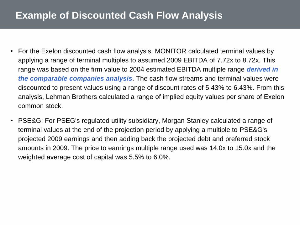
• For the Exelon discounted cash flow analysis, MONITOR calculated terminal values by
applying a range of terminal multiples to assumed 2009 EBITDA of 7.72x to 8.72x. This
range was based on the firm value to 2004 estimated EBITDA multiple range derived in
the comparable companies analysis. The cash flow streams and terminal values were
discounted to present values using a range of discount rates of 5.43% to 6.43%. From this
analysis, Lehman Brothers calculated a range of implied equity values per share of Exelon
common stock.
• PSE&G: For PSEG's regulated utility subsidiary, Morgan Stanley calculated a range of
terminal values at the end of the projection period by applying a multiple to PSE&G's
projected 2009 earnings and then adding back the projected debt and preferred stock
amounts in 2009. The price to earnings multiple range used was 14.0x to 15.0x and the
weighted average cost of capital was 5.5% to 6.0%.

Discounted Cash Flow Analysis – Real World Example
• Credit Suisse First Boston estimated the present value of the stand-alone, Unlevered,
after-tax free cash flows that Texaco could produce over calendar years 2001 through
2004 and that Chevron could produce over the same period. The analysis was based on
estimates of the managements of Texaco and Chevron adjusted, as reviewed by or
discussed with Texaco management, to reflect, among other things, differing
assumptions about future oil and gas prices.
• Ranges of estimated terminal values were calculated by multiplying estimated calendar
year 2004 earnings before interest, taxes, depreciation, amortization and exploration
expense, commonly referred to as EBITDAX, by terminal EBITDAX multiples of 6.5x to
7.5x in the case of both Texaco and Chevron.
• The estimated un-levered after-tax free cash flows and estimated terminal values were
then discounted to present value using discount rates of 9.0 percent to 10.0 percent.
• That analysis indicated an implied exchange ratio reference range of 0.56x to 0.80x.
Problems with Use of Multiples in DCF
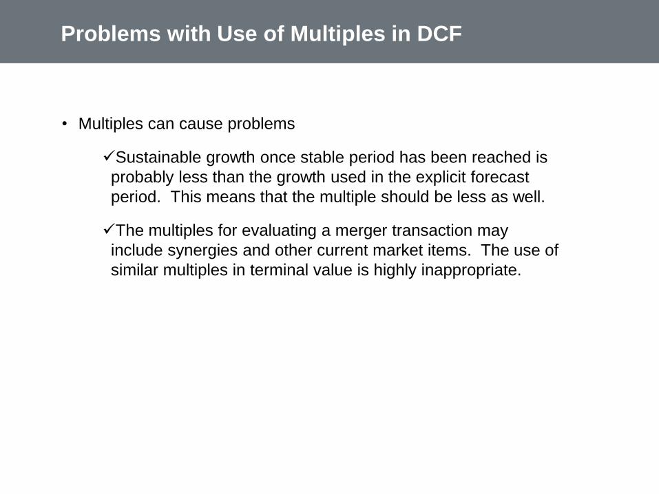
• Multiples can cause problems
Sustainable growth once stable period has been reached is
probably less than the growth used in the explicit forecast
period. This means that the multiple should be less as well.
The multiples for evaluating a merger transaction may
include synergies and other current market items. The use of
similar multiples in terminal value is highly inappropriate.
Continuing Cash Flow from NOPLAT and ROIC
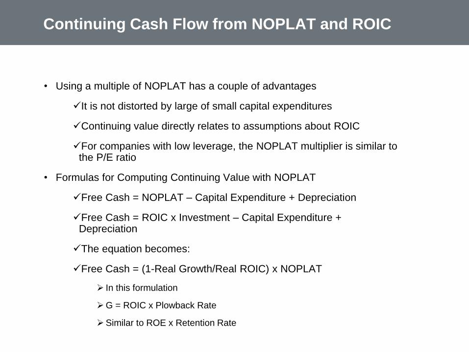
• Using a multiple of NOPLAT has a couple of advantages
It is not distorted by large of small capital expenditures
Continuing value directly relates to assumptions about ROIC
For companies with low leverage, the NOPLAT multiplier is similar to the P/E ratio
• Formulas for Computing Continuing Value with NOPLAT
Free Cash = NOPLAT – Capital Expenditure + Depreciation
Free Cash = ROIC x Investment – Capital Expenditure + Depreciation
The equation becomes:
Free Cash = (1-Real Growth/Real ROIC) x NOPLAT
In this formulation
G = ROIC x Plowback Rate
Similar to ROE x Retention Rate
Reasons for Multiplying by (1+g) in Perpetuity Method
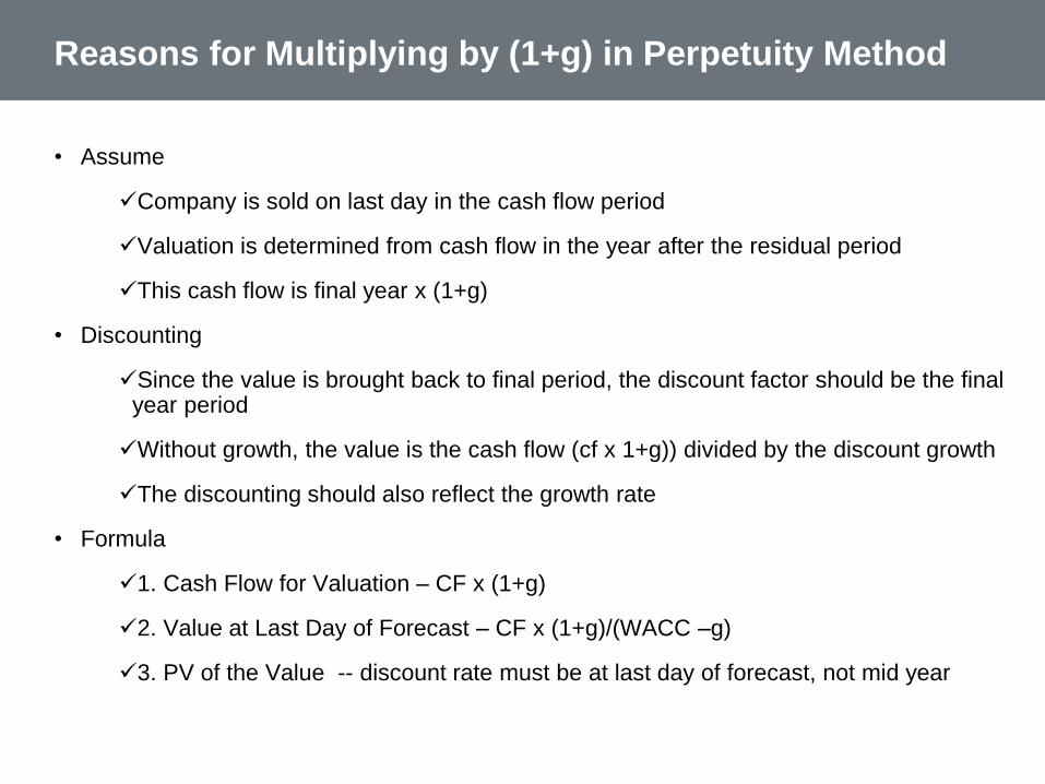
• Assume
Company is sold on last day in the cash flow period
Valuation is determined from cash flow in the year after the residual period
This cash flow is final year x (1+g)
• Discounting
Since the value is brought back to final period, the discount factor should be the final year period
Without growth, the value is the cash flow (cf x 1+g)) divided by the discount growth
The discounting should also reflect the growth rate
• Formula
1. Cash Flow for Valuation – CF x (1+g)
2. Value at Last Day of Forecast – CF x (1+g)/(WACC –g)
3. PV of the Value -- discount rate must be at last day of forecast, not mid year

Formulas for Continuing Value
• A common method for computing cash flow is using the final cash flow in the corporate
model and assuming the company is sold at the end of the
Perpetuity Value at beginning of final year = FCF/WACC
Perpetuity Adjusted for Growth = FCF(1+g)/(WACC - g)
Perpetuity using investment returns =
NOPLAT x (1-g/ROIC)/(WACC - g)
• Once the Perpetuity Value is established for in the last year, it must be discounted to the
current value:
Current Perpetuity Value = PV(Perpetuity Value that occurs at beginning of final
year)
• NPV in excel assumes flows occur at the end of the year. Adjustments can be made to
assume that flows occur in the middle of the year.
In this case, the discounting of the residual is different from discounting of the
individual cash flows
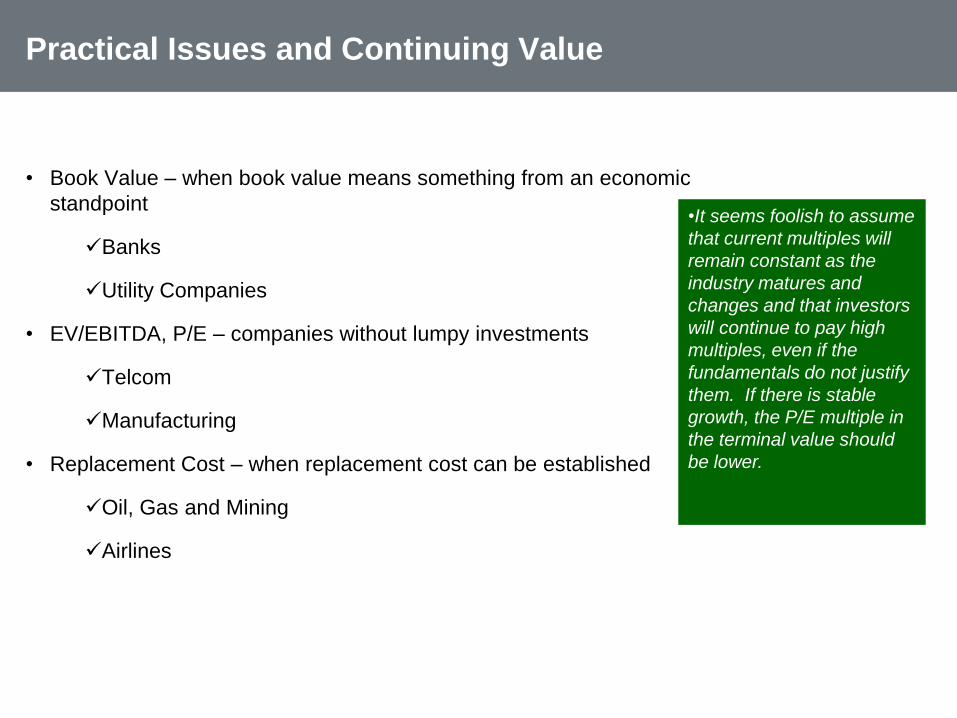
Practical Issues and Continuing Value
• Book Value – when book value means something from an economic
standpoint
Banks
Utility Companies
• EV/EBITDA, P/E – companies without lumpy investments
Telcom
Manufacturing
• Replacement Cost – when replacement cost can be established
Oil, Gas and Mining
Airlines
•It seems foolish to assume
that current multiples will
remain constant as the
industry matures and
changes and that investors
will continue to pay high
multiples, even if the
fundamentals do not justify
them. If there is stable
growth, the P/E multiple in
the terminal value should
be lower.
Issues in Summarising DCF
• Whether to divided by diluted or non-diluted shares depends on
the treatment of employee stock options and convertible bonds
• Work through simple examples
• Three ways to model options
Deduct options from EBITDA and do not use non-diluted
shares – problem, how to handle existing options.
Ignore options and use diluted shares
Explicitly value options as a claim on cash flows and include
as debt – here would use the non-diluted shares
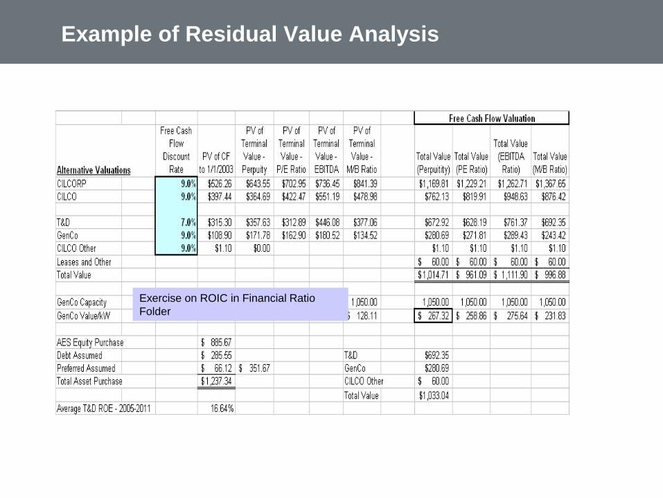
Example of Residual Value Analysis
Exercise on ROIC in Financial Ratio
Folder
Valuation from Projected EPS and Dividend per
Share
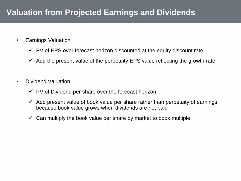
Valuation from Projected Earnings and Dividends
• Earnings Valuation
PV of EPS over forecast horizon discounted at the equity discount rate
Add the present value of the perpetuity EPS value reflecting the growth rate
• Dividend Valuation
PV of Dividend per share over the forecast horizon
Add present value of book value per share rather than perpetuity of earnings because book value grows when dividends are not paid
Can multiply the book value per share by market to book multiple
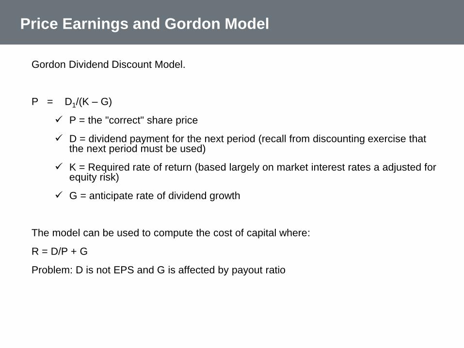
Price Earnings and Gordon Model
Gordon Dividend Discount Model.
P = D1/(K – G)
P = the "correct" share price
D = dividend payment for the next period (recall from discounting exercise that the next period must be used)
K = Required rate of return (based largely on market interest rates a adjusted for equity risk)
G = anticipate rate of dividend growth
The model can be used to compute the cost of capital where:
R = D/P + G
Problem: D is not EPS and G is affected by payout ratio

Illustration of EPS and DPS Valuation
• Demonstrate that incorporation of growth reduces to the formula EPS/(k-g)
• Compute present value of the EPS over the forecast horizon

• Compute free cash flow for segments of the business
• Compute EBITA by segment to evaluate the value with comparables
• Can use different residual value assumptions for different segments of the
business
Corporate Modeling and Valuation of Business Segments
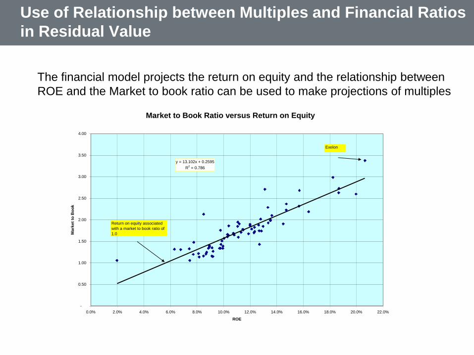
Use of Relationship between Multiples and Financial Ratios
in Residual Value
The financial model projects the return on equity and the relationship between
ROE and the Market to book ratio can be used to make projections of multiples
Market to Book Ratio versus Return on Equity
y = 13.102x + 0.2595
R2 = 0.786
-
0.50
1.00
1.50
2.00
2.50
3.00
3.50
4.00
0.0% 2.0% 4.0% 6.0% 8.0% 10.0% 12.0% 14.0% 16.0% 18.0% 20.0% 22.0%
ROE
Ma
rke
t to
Bo
ok
Return on equity associated
with a market to book ratio of
1.0
Exelon

Example of Business Segment Analysis in Corporate Models
Reference: Selected Valuation Issues

• 1. How do you choose between firm and equity valuation (DCF
valuation versus Earnings Growth)
• Done right, firm and equity valuation should yield the same values for the
equity with consistent assumptions. Choosing between firm (DCF) and equity
valuation (PE x EPS forecasts) boils down to the pragmatic issue of ease.
• For banks, firm valuation does not work because small differences in WACC
can have dramatic effects on valuation while and if the market value of debt
differs from the book value, firm value can cause distortions.
Valuation Issues
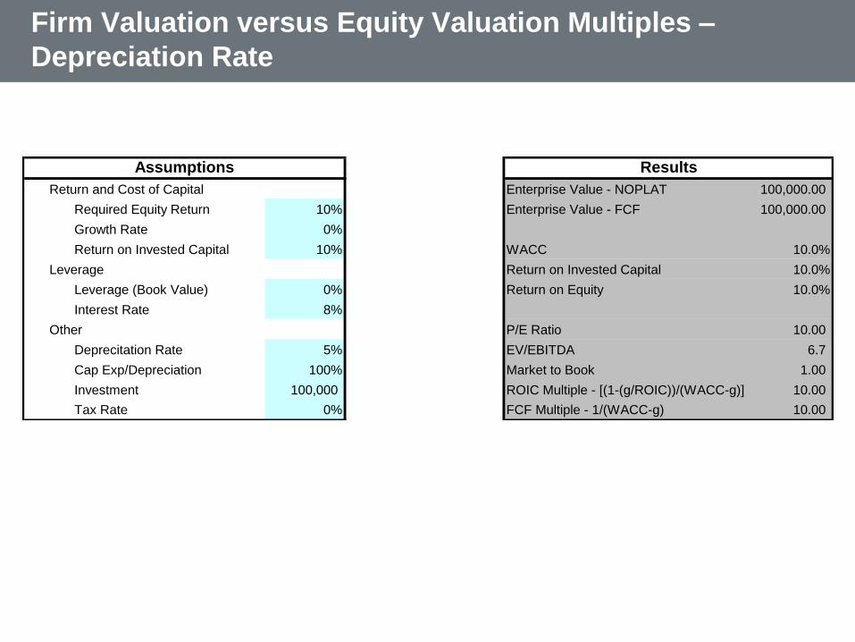
Firm Valuation versus Equity Valuation Multiples –
Depreciation Rate
Return and Cost of Capital Enterprise Value - NOPLAT 100,000.00
Required Equity Return 10% Enterprise Value - FCF 100,000.00
Growth Rate 0%
Return on Invested Capital 10% WACC 10.0%
Leverage Return on Invested Capital 10.0%
Leverage (Book Value) 0% Return on Equity 10.0%
Interest Rate 8%
Other P/E Ratio 10.00
Deprecitation Rate 5% EV/EBITDA 6.7
Cap Exp/Depreciation 100% Market to Book 1.00
Investment 100,000 ROIC Multiple - [(1-(g/ROIC))/(WACC-g)] 10.00
Tax Rate 0% FCF Multiple - 1/(WACC-g) 10.00
ResultsAssumptions

Equity vs Firm Valuation – Income Taxes and Depreciation
Return and Cost of Capital Enterprise Value - NOPLAT 100,000.00
Required Equity Return 10% Enterprise Value - FCF 100,000.00
Growth Rate 0%
Return on Invested Capital 10% WACC 10.0%
Leverage Return on Invested Capital 10.0%
Leverage (Book Value) 0% Return on Equity 10.0%
Interest Rate 8%
Other P/E Ratio 10.00
Deprecitation Rate 5% EV/EBITDA 5.2
Cap Exp/Depreciation 100% Market to Book 1.00
Investment 100,000 ROIC Multiple - [(1-(g/ROIC))/(WACC-g)] 10.00
Tax Rate 30% FCF Multiple - 1/(WACC-g) 10.00
ResultsAssumptions
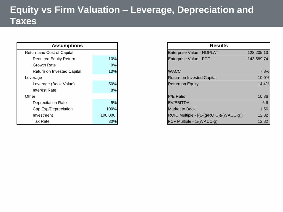
Equity vs Firm Valuation – Leverage, Depreciation and
Taxes
Return and Cost of Capital Enterprise Value - NOPLAT 128,205.13
Required Equity Return 10% Enterprise Value - FCF 143,589.74
Growth Rate 0%
Return on Invested Capital 10% WACC 7.8%
Leverage Return on Invested Capital 10.0%
Leverage (Book Value) 50% Return on Equity 14.4%
Interest Rate 8%
Other P/E Ratio 10.86
Deprecitation Rate 5% EV/EBITDA 6.6
Cap Exp/Depreciation 100% Market to Book 1.56
Investment 100,000 ROIC Multiple - [(1-(g/ROIC))/(WACC-g)] 12.82
Tax Rate 30% FCF Multiple - 1/(WACC-g) 12.82
ResultsAssumptions
• From the perspective of convenience, it is often easier to estimate equity
than the DCF, especially when leverage is changing significantly over
time (for example, in project finance and in leveraged buyouts where
equity IRR is used).
• Equity value measures a real cash flow to owners, rather than an
abstraction (free cash flows to the firm exist only on paper). Free cash
flow is affected to a large extent by capital expenditures which can cause
problems.
Firm versus Equity Valuation
• While there are many who use historical (past) growth as a
measure of expected growth, or choose to trust analysts
(with their projections), try using fundamentals.
• Think about the two factors that determine growth - the firm's
reinvestment policy and its rate of return.
For expected growth in earnings = Retention Ratio * ROE,
where Retention Ratio is 1 – Dividend Payout
For expected growth in EBIT = Reinvestment Rate * ROC,
where reinvestment rate is Cap Exp/Depreciation
Measurement of Expected Growth Rate

At 100% Payout – Growth Equals ROE
Price to Earnings ComputationLong-Term Growth Rate 0.00% Total Value (Sum of Annual Value) 5.96
Long-Term Return Return on Equity 15.0% Initial Earnings 1.03
Equity Cost of Capital 15.0% PE Ratio - Value/Net Income 5.80
P/E Formula: (1-g/r)/(k-g) 6.67 PEG: PE/Growth 0.39
Year 1 2 3 4 5 6 7 8 9
Return on Equity 15.00% 15.00% 15.00% 15.00% 15.00% 15.00% 15.00% 15.00% 15.00%
Dividend Payout 0.00% 0.00% 0.00% 0.00% 0.00% 0.00% 0.00% 0.00% 0.00%
Holding Period 10
Switch for Terminal Period FALSE FALSE FALSE FALSE FALSE FALSE FALSE FALSE FALSE
Switch for Cash Flow Period TRUE TRUE TRUE TRUE TRUE TRUE TRUE TRUE TRUE
InvestmentBeginning Investment 6.85
Beginning Equity (Last Period Ending) 6.85 7.88 9.06 10.42 11.98 13.78 15.84 18.22 20.95
Add: Earnings (ROE x Beginning Equity) 1.03 1.18 1.36 1.56 1.80 2.07 2.38 2.73 3.14
Less: Dividends (NI x Payout Ratio) - - - - - - - - -
Ending Equity (Beg + Income - Payout) 7.88 9.06 10.42 11.98 13.78 15.84 18.22 20.95 24.10
Cash Flow to Equity and ValuationCash flow from Dividends from Above - - - - - - - - -
Terminal Multiple of Earnings from Above 6.67 6.67 6.67 6.67 6.67 6.67 6.67 6.67 6.67
Terminal Cash Flow (Earnings x Mult x (1+g)) - - - - - - - - -
Total Cash Flow (Terminal + Dividends) - - - - - - - - -
Required Return on Equity 15.00% 15.0% 15.0% 15.0% 15.0% 15.0% 15.0% 15.0% 15.0%
Discount Factor [1/(required return + 1)^yr] 0.87 0.76 0.66 0.57 0.50 0.43 0.38 0.33 0.28
Value of Cash Flow [CF x Discount Fac] x Switch - - - - - - - - -
Period Future Earn Current Growth
10 3.61 1.03 15.00%
Growth over Forecast Horizon
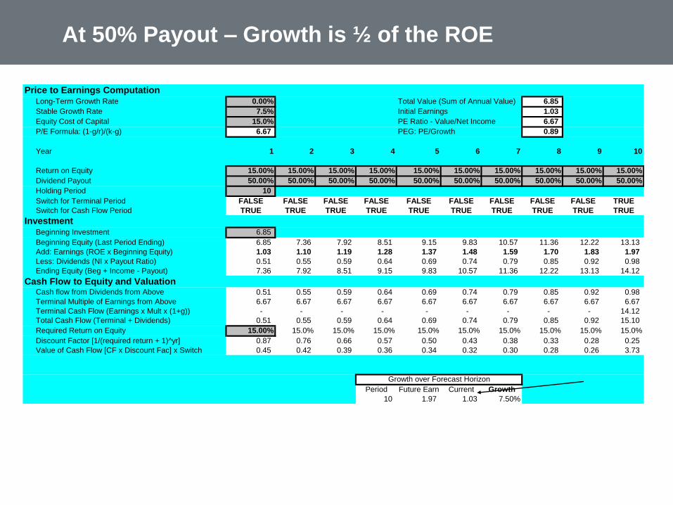
At 50% Payout – Growth is ½ of the ROE
Price to Earnings ComputationLong-Term Growth Rate 0.00% Total Value (Sum of Annual Value) 6.85
Stable Growth Rate 7.5% Initial Earnings 1.03
Equity Cost of Capital 15.0% PE Ratio - Value/Net Income 6.67
P/E Formula: (1-g/r)/(k-g) 6.67 PEG: PE/Growth 0.89
Year 1 2 3 4 5 6 7 8 9 10
Return on Equity 15.00% 15.00% 15.00% 15.00% 15.00% 15.00% 15.00% 15.00% 15.00% 15.00%
Dividend Payout 50.00% 50.00% 50.00% 50.00% 50.00% 50.00% 50.00% 50.00% 50.00% 50.00%
Holding Period 10
Switch for Terminal Period FALSE FALSE FALSE FALSE FALSE FALSE FALSE FALSE FALSE TRUE
Switch for Cash Flow Period TRUE TRUE TRUE TRUE TRUE TRUE TRUE TRUE TRUE TRUE
InvestmentBeginning Investment 6.85
Beginning Equity (Last Period Ending) 6.85 7.36 7.92 8.51 9.15 9.83 10.57 11.36 12.22 13.13
Add: Earnings (ROE x Beginning Equity) 1.03 1.10 1.19 1.28 1.37 1.48 1.59 1.70 1.83 1.97
Less: Dividends (NI x Payout Ratio) 0.51 0.55 0.59 0.64 0.69 0.74 0.79 0.85 0.92 0.98
Ending Equity (Beg + Income - Payout) 7.36 7.92 8.51 9.15 9.83 10.57 11.36 12.22 13.13 14.12
Cash Flow to Equity and ValuationCash flow from Dividends from Above 0.51 0.55 0.59 0.64 0.69 0.74 0.79 0.85 0.92 0.98
Terminal Multiple of Earnings from Above 6.67 6.67 6.67 6.67 6.67 6.67 6.67 6.67 6.67 6.67
Terminal Cash Flow (Earnings x Mult x (1+g)) - - - - - - - - - 14.12
Total Cash Flow (Terminal + Dividends) 0.51 0.55 0.59 0.64 0.69 0.74 0.79 0.85 0.92 15.10
Required Return on Equity 15.00% 15.0% 15.0% 15.0% 15.0% 15.0% 15.0% 15.0% 15.0% 15.0%
Discount Factor [1/(required return + 1)^yr] 0.87 0.76 0.66 0.57 0.50 0.43 0.38 0.33 0.28 0.25
Value of Cash Flow [CF x Discount Fac] x Switch 0.45 0.42 0.39 0.36 0.34 0.32 0.30 0.28 0.26 3.73
Period Future Earn Current Growth
10 1.97 1.03 7.50%
Growth over Forecast Horizon
• Note that what we really need to estimate are reinvestment rates and
marginal returns on equity and capital in the future (the change in
Income over the change in Equity).
• Note that those who use analyst’s or historical growth rates are implicitly
assuming something about reinvestment rates and returns, but they are
either unaware of these assumptions or do not make them explicit. This
means, look at the ROE and the dividends to make sure that the growth
is consistent.
• Future ROE depends on changes in economic variables affecting the
existing investment and new projects with incremental returns.
Growth Rate Estimation vs ROE and Retention Rate

How Long will Growth Last
• There is no single answer to the question, so look at the following characteristics:
• A. The greater the current growth rate in earnings of a firm, relative to the stable growth rate,
the longer the high growth period; although the growth rate may drop off during the period.
Thus, a firm that is growing at 40% should have a longer high-growth period than one growing
at 14%.
• B. The larger the size of the firm, the shorter the high growth period. Size remains one of the
most potent forces that push firms towards stable growth; the larger a firm, the less likely it is to
maintain an above-normal growth rate.
• C. The greater the barriers to entry in a business, e.g. patents or strong brand name, should
lengthen the high growth period for a firm.
• Look at the combination of the three factors A,B,C and make a judgment. Few firms can
achieve an expected growth period longer than 10 years

Effect of Growth – Microsoft Example – Long-term Equals
the Current Growth – P/E is 20
Price to Earnings ComputationLong-Term Growth Rate 7.50% Total Value (Sum of Annual Value) 20.55
Long-term Return 15.0% Initial Earnings 1.03
Equity Cost of Capital 10.0% PE Ratio - Value/Net Income 20.00
P/E Formula: (1-g/r)/(k-g) 20.00 PEG: PE/Growth 2.67
Year 1 2 3 4 5 6 7 8 9 10
Return on Equity 15.00% 15.00% 15.00% 15.00% 15.00% 15.00% 15.00% 15.00% 15.00% 15.00%
Dividend Payout 50.00% 50.00% 50.00% 50.00% 50.00% 50.00% 50.00% 50.00% 50.00% 50.00%
Holding Period 10
Switch for Terminal Period FALSE FALSE FALSE FALSE FALSE FALSE FALSE FALSE FALSE TRUE
Switch for Cash Flow Period TRUE TRUE TRUE TRUE TRUE TRUE TRUE TRUE TRUE TRUE
InvestmentBeginning Investment 6.85
Beginning Equity (Last Period Ending) 6.85 7.36 7.92 8.51 9.15 9.83 10.57 11.36 12.22 13.13
Add: Earnings (ROE x Beginning Equity) 1.03 1.10 1.19 1.28 1.37 1.48 1.59 1.70 1.83 1.97
Less: Dividends (NI x Payout Ratio) 0.51 0.55 0.59 0.64 0.69 0.74 0.79 0.85 0.92 0.98
Ending Equity (Beg + Income - Payout) 7.36 7.92 8.51 9.15 9.83 10.57 11.36 12.22 13.13 14.12
Cash Flow to Equity and ValuationCash flow from Dividends from Above 0.51 0.55 0.59 0.64 0.69 0.74 0.79 0.85 0.92 0.98
Terminal Multiple of Earnings from Above 20.00 20.00 20.00 20.00 20.00 20.00 20.00 20.00 20.00 20.00
Terminal Cash Flow (Earnings x Mult x (1+g)) - - - - - - - - - 42.35
Total Cash Flow (Terminal + Dividends) 0.51 0.55 0.59 0.64 0.69 0.74 0.79 0.85 0.92 43.34
Required Return on Equity 10.00% 10.0% 10.0% 10.0% 10.0% 10.0% 10.0% 10.0% 10.0% 10.0%
Discount Factor [1/(required return + 1)^yr] 0.91 0.83 0.75 0.68 0.62 0.56 0.51 0.47 0.42 0.39
Value of Cash Flow [CF x Discount Fac] x Switch 0.47 0.46 0.45 0.44 0.43 0.42 0.41 0.40 0.39 16.71
Period Future Earn Current Growth
10 1.97 1.03 7.50%
Growth over Forecast Horizon
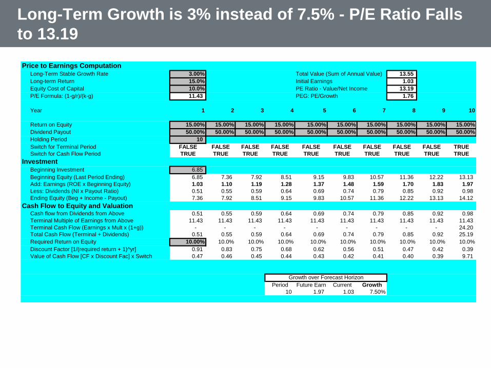
Long-Term Growth is 3% instead of 7.5% - P/E Ratio Falls
to 13.19
Price to Earnings ComputationLong-Term Stable Growth Rate 3.00% Total Value (Sum of Annual Value) 13.55
Long-term Return 15.0% Initial Earnings 1.03
Equity Cost of Capital 10.0% PE Ratio - Value/Net Income 13.19
P/E Formula: (1-g/r)/(k-g) 11.43 PEG: PE/Growth 1.76
Year 1 2 3 4 5 6 7 8 9 10
Return on Equity 15.00% 15.00% 15.00% 15.00% 15.00% 15.00% 15.00% 15.00% 15.00% 15.00%
Dividend Payout 50.00% 50.00% 50.00% 50.00% 50.00% 50.00% 50.00% 50.00% 50.00% 50.00%
Holding Period 10
Switch for Terminal Period FALSE FALSE FALSE FALSE FALSE FALSE FALSE FALSE FALSE TRUE
Switch for Cash Flow Period TRUE TRUE TRUE TRUE TRUE TRUE TRUE TRUE TRUE TRUE
InvestmentBeginning Investment 6.85
Beginning Equity (Last Period Ending) 6.85 7.36 7.92 8.51 9.15 9.83 10.57 11.36 12.22 13.13
Add: Earnings (ROE x Beginning Equity) 1.03 1.10 1.19 1.28 1.37 1.48 1.59 1.70 1.83 1.97
Less: Dividends (NI x Payout Ratio) 0.51 0.55 0.59 0.64 0.69 0.74 0.79 0.85 0.92 0.98
Ending Equity (Beg + Income - Payout) 7.36 7.92 8.51 9.15 9.83 10.57 11.36 12.22 13.13 14.12
Cash Flow to Equity and ValuationCash flow from Dividends from Above 0.51 0.55 0.59 0.64 0.69 0.74 0.79 0.85 0.92 0.98
Terminal Multiple of Earnings from Above 11.43 11.43 11.43 11.43 11.43 11.43 11.43 11.43 11.43 11.43
Terminal Cash Flow (Earnings x Mult x (1+g)) - - - - - - - - - 24.20
Total Cash Flow (Terminal + Dividends) 0.51 0.55 0.59 0.64 0.69 0.74 0.79 0.85 0.92 25.19
Required Return on Equity 10.00% 10.0% 10.0% 10.0% 10.0% 10.0% 10.0% 10.0% 10.0% 10.0%
Discount Factor [1/(required return + 1)^yr] 0.91 0.83 0.75 0.68 0.62 0.56 0.51 0.47 0.42 0.39
Value of Cash Flow [CF x Discount Fac] x Switch 0.47 0.46 0.45 0.44 0.43 0.42 0.41 0.40 0.39 9.71
Period Future Earn Current Growth
10 1.97 1.03 7.50%
Growth over Forecast Horizon
• Terminal value refers to the value of the firm (or equity) at the
end of the high growth period. Estimate terminal value, with
DCF, by assuming a stable growth rate that the firm can
sustain forever. If we make this assumption, the terminal
value becomes:
• Terminal Value in year n = Cash Flow in year n+1 / (r - g)
• This approach requires the assumption that growth is
constant forever, and that the cost of capital will not change
over time.
Estimation of Terminal Value

• A stable growth rate is a growth rate that can be sustained forever. Since no
firm, in the long term, can grow faster than the economy which it operates it -
a stable growth rate cannot be greater than the growth rate of the economy.
• It is important that the growth rate be defined in the same currency as the
cash flows and that be in the same term (real or nominal) as the cash flows.
• In theory, this stable growth rate cannot be greater than the discount rate
because the risk-free rate that is embedded in the discount rate will also build
on these same factors - real growth in the economy and the expected
inflation rate.
Growth Rate and Discount Rate
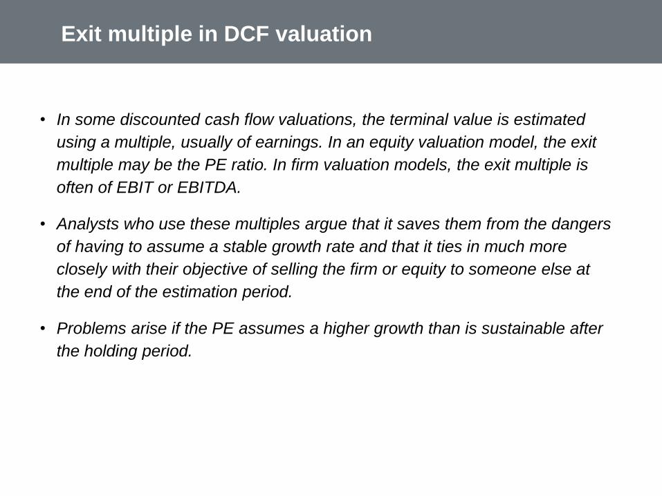
• In some discounted cash flow valuations, the terminal value is estimated
using a multiple, usually of earnings. In an equity valuation model, the exit
multiple may be the PE ratio. In firm valuation models, the exit multiple is
often of EBIT or EBITDA.
• Analysts who use these multiples argue that it saves them from the dangers
of having to assume a stable growth rate and that it ties in much more
closely with their objective of selling the firm or equity to someone else at
the end of the estimation period.
• Problems arise if the PE assumes a higher growth than is sustainable after
the holding period.
Exit multiple in DCF valuation
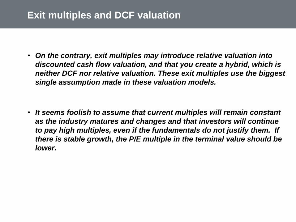
• On the contrary, exit multiples may introduce relative valuation into
discounted cash flow valuation, and that you create a hybrid, which is
neither DCF nor relative valuation. These exit multiples use the biggest
single assumption made in these valuation models.
• It seems foolish to assume that current multiples will remain constant
as the industry matures and changes and that investors will continue
to pay high multiples, even if the fundamentals do not justify them. If
there is stable growth, the P/E multiple in the terminal value should be
lower.
Exit multiples and DCF valuation
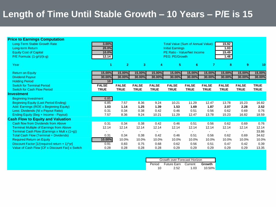
Length of Time Until Stable Growth – 10 Years – P/E is 15
Price to Earnings ComputationLong-Term Stable Growth Rate 3.00% Total Value (Sum of Annual Value) 15.92
Long-term Return 20.0% Initial Earnings 1.03
Equity Cost of Capital 10.0% PE Ratio - Value/Net Income 15.49
P/E Formula: (1-g/r)/(k-g) 12.14 PEG: PE/Growth 1.48
Year 1 2 3 4 5 6 7 8 9 10
Return on Equity 15.00% 15.00% 15.00% 15.00% 15.00% 15.00% 15.00% 15.00% 15.00% 15.00%
Dividend Payout 30.00% 30.00% 30.00% 30.00% 30.00% 30.00% 30.00% 30.00% 30.00% 30.00%
Holding Period 10
Switch for Terminal Period FALSE FALSE FALSE FALSE FALSE FALSE FALSE FALSE FALSE TRUE
Switch for Cash Flow Period TRUE TRUE TRUE TRUE TRUE TRUE TRUE TRUE TRUE TRUE
InvestmentBeginning Investment 6.85
Beginning Equity (Last Period Ending) 6.85 7.57 8.36 9.24 10.21 11.29 12.47 13.78 15.23 16.82
Add: Earnings (ROE x Beginning Equity) 1.03 1.14 1.25 1.39 1.53 1.69 1.87 2.07 2.28 2.52
Less: Dividends (NI x Payout Ratio) 0.31 0.34 0.38 0.42 0.46 0.51 0.56 0.62 0.69 0.76
Ending Equity (Beg + Income - Payout) 7.57 8.36 9.24 10.21 11.29 12.47 13.78 15.23 16.82 18.59
Cash Flow to Equity and ValuationCash flow from Dividends from Above 0.31 0.34 0.38 0.42 0.46 0.51 0.56 0.62 0.69 0.76
Terminal Multiple of Earnings from Above 12.14 12.14 12.14 12.14 12.14 12.14 12.14 12.14 12.14 12.14
Terminal Cash Flow (Earnings x Mult x (1+g)) - - - - - - - - - 33.86
Total Cash Flow (Terminal + Dividends) 0.31 0.34 0.38 0.42 0.46 0.51 0.56 0.62 0.69 34.62
Required Return on Equity 10.00% 10.0% 10.0% 10.0% 10.0% 10.0% 10.0% 10.0% 10.0% 10.0%
Discount Factor [1/(required return + 1)^yr] 0.91 0.83 0.75 0.68 0.62 0.56 0.51 0.47 0.42 0.39
Value of Cash Flow [CF x Discount Fac] x Switch 0.28 0.28 0.28 0.28 0.29 0.29 0.29 0.29 0.29 13.35
Period Future Earn Current Growth
10 2.52 1.03 10.50%
Growth over Forecast Horizon
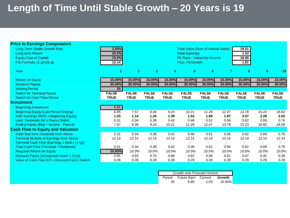
Length of Time Until Stable Growth – 20 Years is 19
Price to Earnings ComputationLong-Term Stable Growth Rate 3.00% Total Value (Sum of Annual Value) 19.51
Long-term Return 20.0% Initial Earnings 1.03
Equity Cost of Capital 10.0% PE Ratio - Value/Net Income 18.99
P/E Formula: (1-g/r)/(k-g) 12.14 PEG: PE/Growth 1.81
Year 1 2 3 4 5 6 7 8 9 10
Return on Equity 15.00% 15.00% 15.00% 15.00% 15.00% 15.00% 15.00% 15.00% 15.00% 15.00%
Dividend Payout 30.00% 30.00% 30.00% 30.00% 30.00% 30.00% 30.00% 30.00% 30.00% 30.00%
Holding Period 20
Switch for Terminal Period FALSE FALSE FALSE FALSE FALSE FALSE FALSE FALSE FALSE FALSE
Switch for Cash Flow Period TRUE TRUE TRUE TRUE TRUE TRUE TRUE TRUE TRUE TRUE
InvestmentBeginning Investment 6.85
Beginning Equity (Last Period Ending) 6.85 7.57 8.36 9.24 10.21 11.29 12.47 13.78 15.23 16.82
Add: Earnings (ROE x Beginning Equity) 1.03 1.14 1.25 1.39 1.53 1.69 1.87 2.07 2.28 2.52
Less: Dividends (NI x Payout Ratio) 0.31 0.34 0.38 0.42 0.46 0.51 0.56 0.62 0.69 0.76
Ending Equity (Beg + Income - Payout) 7.57 8.36 9.24 10.21 11.29 12.47 13.78 15.23 16.82 18.59
Cash Flow to Equity and ValuationCash flow from Dividends from Above 0.31 0.34 0.38 0.42 0.46 0.51 0.56 0.62 0.69 0.76
Terminal Multiple of Earnings from Above 12.14 12.14 12.14 12.14 12.14 12.14 12.14 12.14 12.14 12.14
Terminal Cash Flow (Earnings x Mult x (1+g)) - - - - - - - - - -
Total Cash Flow (Terminal + Dividends) 0.31 0.34 0.38 0.42 0.46 0.51 0.56 0.62 0.69 0.76
Required Return on Equity 10.00% 10.0% 10.0% 10.0% 10.0% 10.0% 10.0% 10.0% 10.0% 10.0%
Discount Factor [1/(required return + 1)^yr] 0.91 0.83 0.75 0.68 0.62 0.56 0.51 0.47 0.42 0.39
Value of Cash Flow [CF x Discount Fac] x Switch 0.28 0.28 0.28 0.28 0.29 0.29 0.29 0.29 0.29 0.29
Period Future Earn Current Growth
20 6.85 1.03 10.50%
Growth over Forecast Horizon

• These models have assumptions about net capital expenditures and growth that
are strongly linked. When one changes, so should the other. There are two types
of errors that show up in these valuations.
• First, high growth firms with high net capital expenditures are assumed to keep
reinvesting at current rates, even as growth drops off. Not surprisingly, these
firms are not valued very highly in these models.
• Second, the net capital expenditures are reduced to zero in stable growth, even
as the firm is assumed to grow at some rate forever. Here, the valuations tend to
be too high.
Avoid errors and make the assumptions about reinvestment a function of the
growth and the return on capital. As growth changes, the reinvestment rate must
change.
Common errors in FCFE/FCFF model valuation
• There are a number of reasons why a firm might have negative earnings,
and the response will vary depending upon the reason:
- If the earnings of a cyclical firm are depressed due to a recession, the
best response is to normalize earnings by taking the average earnings
over a entire business cycle.
- Normalized Net Income = Average ROE * Current Book Value of Equity
- Normalized after-tax Operating Income = Average ROC * Current Book
Value of Assets
- Once earnings are normalized, the growth rate used should be
consistent with the normalized earnings, and should reflect the real
growth potential of the firm rather than the cyclical effects.
Valuation of Firms that are Losing Money

- If the earnings of a firm are depressed due to a one-time charge, the best
response is to estimate the earnings without the one-time charge and value the firm
based upon these earnings.
- If the earnings of a firm are depressed due to poor quality management, the
average return on equity or capital for the industry can be used to estimate
normalized earnings for the firm. The implicit assumption is that the firm will recover
back to industry averages, once management has been removed.
- Normalized Net Income = Industry-average ROE * Current Book Value of Equity
- Normalized after-tax Operating Income = Industry-average ROC * Current Book Value of
Assets
Valuation of a firm that is Losing Money
• - If the negative earnings over time have caused the book value to decline
significantly over time, use the average operating or profit margins for the
industry in conjunction with revenues to arrive at normalized earnings. Thus,
a firm with negative operating income today could be assumed to converge
on the normalized earnings five years from now. - If the earnings of a firm are
depressed or negative because it operates in a sector which is in its early
stages of its life cycle, the discounted cash flow valuation will be driven by
the perception of what the operating margins and returns on equity (capital)
will be when the sector matures.
• - If the equity earnings are depressed due to high leverage, the best solution
is to value the firm rather than just the equity, factoring in the reduction in
leverage over time.
Valuation of a firm that is losing money
• The valuation of a private firm is more difficult than stock in a
publicly traded firm. In particular,
A. The information available on private firms will be sketchier
than the information available on publicly traded firms.
B. Past financial statements, even when available, might not
reflect the true earnings potential of the firm. Many private
businesses understate earnings to reduce their tax liabilities,
and the expenses at many private businesses often reflect
the blurring of lines between private and business expenses.
Valuation of a private firms
C. The owners of many private businesses are taxed on the salary they
make and the dividends they take out of the business; often do not try to
distinguish between the two.
The limited availability of information does make the estimation of cash
flows impossible; past financial statements might need to be restated to
make them reflect the true earnings of the firm.
Once the cash flows are estimated, the choice of a discount rate might be
affected by the identity of the potential buyer of the business. If the
potential buyer of the business is a publicly traded firm, the valuation
should be done using the discount rates based upon market risk
Valuation of a private firm

EPS Measures – Establishing a reliable starting point
• Reported EPS – EPS reported by the company using generally accepted
accounting principles. Therefore includes earnings from recurring and non-
recurring items
• Recurring EPS – Reported EPS adjusted to exclude non-recurring items
• Fully diluted EPS – EPS adjusted to reflect dilution to existing shareholders as a
result of future increases in equity shares

EPS adjustments
Item
For recurring
net profit
For
‘economic profit’
Profits and losses on operations discontinued during the period IN OUT
Profits or losses on disposals of investments acquired for resale but not
held in the ordinary course of business IN OUT
Extraordinary items OUT OUT
Gains or losses on the disposal of fixed assets IN IN
Gains or losses on the disposal of subsidiaries/associates or business units OUT OUT
Goodwill amortisation OUT OUT
Provisions for reorganisation or restructuring IN OUT
Note: adjustments only made to the extent disclosure allows and materiality equires
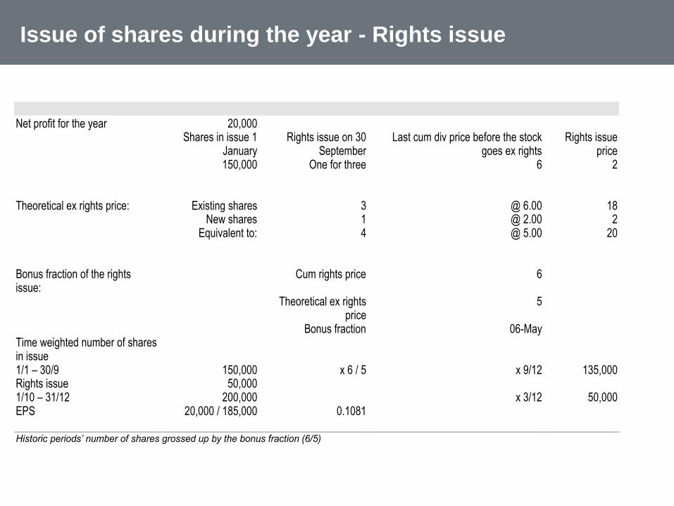
Net profit for the year 20,000 Shares in issue 1
January Rights issue on 30
September Last cum div price before the stock
goes ex rights Rights issue
price 150,000 One for three 6 2
Theoretical ex rights price: Existing shares 3 @ 6.00 18 New shares 1 @ 2.00 2 Equivalent to: 4 @ 5.00 20
Bonus fraction of the rights issue:
Cum rights price 6
Theoretical ex rights price
5
Bonus fraction 06-May Time weighted number of shares in issue
1/1 – 30/9 150,000 x 6 / 5 x 9/12 135,000 Rights issue 50,000 1/10 – 31/12 200,000 x 3/12 50,000 EPS 20,000 / 185,000 0.1081
Historic periods’ number of shares grossed up by the bonus fraction (6/5)
Issue of shares during the year - Rights issue

Date Shares Weighted Average
Start of year 200 million x 6/12 100 million
After Buy Back 180 million x 6/12 90 million
Weighted Average 190 million
EPS = $33 million/ 190 million = 17. 3 CENTS
Share buy back
• Redeem Ltd made earnings of $ 33 million dollars for the year
ended March 2004. The number of shares issued at the start of
the year was 200 million. In September 2003 Redeem Ltd bought
back 20 million shares at market price.
Dilution – Factors and treatment
• Contingently issuable shares - Include shares in the calculation of
basic EPS if the contingency has been met.
• Options or warrants in existence over as yet un-issued shares –
Assume exercise of outstanding dilutive options and warrants
• Loan stock or preference shares convertible into equity shares in
the future – Assume that instruments are converted therefore
saving interest but increasing the number of shares in issue

Diluted Shares
• If you have agreed to give away shares to someone, then your
claim to the cash flow of the company is reduced.
• In the extreme, if you have given away half of your company
away, and the cash flow is the same before and after your give
away, then the amount you would pay for the share must account
for how much you will give away.
• In this extreme example, you should reduce the value by ½.
• This can be accomplished by using diluted shares rather than
basic shares.

Option dilution
• Calculation of the number of shares in the dilution calculation is
illustrated below:

Equivalence factor approach
Net Profit $300,000
Par value No. Total par value Price
Class A Primary $5.00 800,000 $4,000,000 $10
Class B Secondary $0.50 4,000,000 $2,000,000 $1.2
$6,000,000
Secondary to primary equivalence factor 0.1
Equivalent number of primary shares 1,200,000
Class A EPS 25.00c (300,000 / 1,2000,000)
Class A PE 40.00x (10.00 / 0.25)
Class B EPS 2.5 Class A EPS x equivalence factor
Class B PE 48.00x (10.00 / 0.25)
Multiple share classes

State
owned
“H” Shares “A” Shares Total
Number ( million) 300 156.7 30 486.7
Price - local HKD 1.50 RMB 5
Price - RMB 1.58 5
Equity Value – RMB million 769 2433
Multiple Listings
Fungible shares listed on different exchanges – EPS calculated on the basis of
total shares - Value equity based on shares held by the investor group to
whom your research is directed
Issues in the application of PEs
• Accounting Policy differences – Particularly significant for cross border comparisons
where companies may follow local, international or US GAAP
• Loss making companies – No earnings therefore no PE
• Cyclical companies – PEs volatile through the cycle and therefore difficult to benchmark
• Finding a suitable benchmark – Difficult to find companies that are perfect matches in all
determinants of a PE
• Growth – As discussed value and growth are not always the same
• Capital market conditions – The cost of equity will vary depending on underlying interest
rate environment that is likely to be different in different countries
• Financing – The greater the gearing of a company the greater the cost of equity and
therefore, all other things being equal, the lower the value and the lower the PE
Valuation of Subsidiary Companies in Different Countries
• How would things differ if we are valuing companies from different countries, different
sectors etc.
• The basic rule is:
Cash flows should be nominal
Cash flows should be stated in the currency where the subsidiary is located
If there are multiple currencies, use the future expected spot exchange rates to translate cash
flows
Cash flows should be discounted at cost of capital that reflects the interest rates where
the country is located
This means that the risk free rate in the country where the subsidiary is located should be
used.
Once the value is established, translate the amount to the home country at the spot
exchange rate
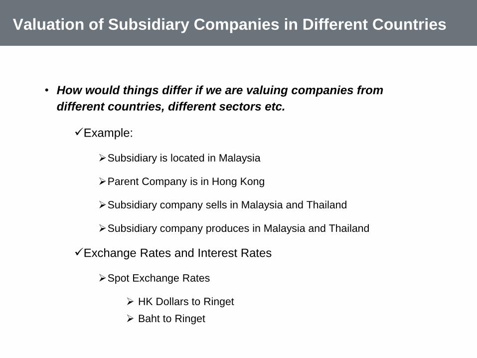
Valuation of Subsidiary Companies in Different Countries
• How would things differ if we are valuing companies from
different countries, different sectors etc.
Example:
Subsidiary is located in Malaysia
Parent Company is in Hong Kong
Subsidiary company sells in Malaysia and Thailand
Subsidiary company produces in Malaysia and Thailand
Exchange Rates and Interest Rates
Spot Exchange Rates
HK Dollars to Ringet
Baht to Ringet

Valuation of Subsidiary Companies in Different Countries
• How would things differ if we are valuing companies from different countries,
different sectors etc.
• Cash flows should be stated in the currency where the subsidiary is located (Malaysian
Ringgit)
Compute prices and costs in Baht and Ringgit and then translate the revenues and
costs in Baht to Ringgit
To convert the Baht to Ringgit, use the expected future spot Ringet/Baht exchange
rates
Since, as a practical matter, forward exchange rates are not available beyond 18
months, compute future spot rates from interest rate parity
Interest rate parity means that if you invest in risk free securities of different
currencies, the spot exchange rate must reflect the future values.
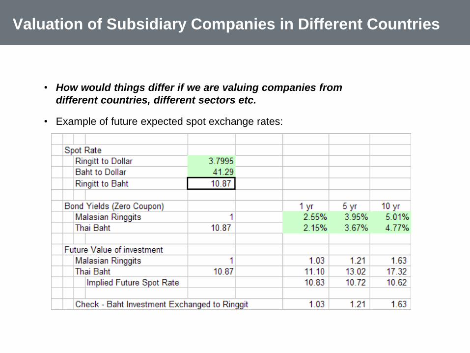
Valuation of Subsidiary Companies in Different Countries
• How would things differ if we are valuing companies from
different countries, different sectors etc.
• Example of future expected spot exchange rates:

Example of Foreign Valuation

Free Cash Flow
We often talk about free cash flow, sometimes, it is challenging to assess
what is "free“ cash flow or not, may wish to elaborate on that rather than
just defining free cash flow in a text book term.
The basic point is to keep things consistent. If you define FCF as EBITDA
without other income, then the valuation does not include other investments.
On the other hand if FCF is defined using Cash B/4 Financing that includes other
income, the other investments are included in the valuation
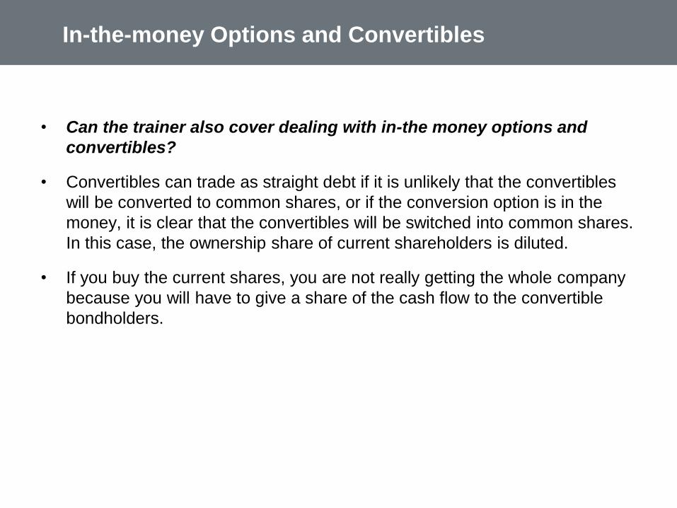
In-the-money Options and Convertibles
• Can the trainer also cover dealing with in-the money options and
convertibles?
• Convertibles can trade as straight debt if it is unlikely that the convertibles
will be converted to common shares, or if the conversion option is in the
money, it is clear that the convertibles will be switched into common shares.
In this case, the ownership share of current shareholders is diluted.
• If you buy the current shares, you are not really getting the whole company
because you will have to give a share of the cash flow to the convertible
bondholders.

Terminal Value
• Terminal value, and the use of a stable growth rate. How do you determine that, what is
the rule of thumb and how do you determine which year onwards should be terminal year
(i.e. how long should your forecasted period be).
• On how to calculate a WACC, rather than just providing the formula of WACC, it would be
useful to give instructions on where to find the market premium data, betas and what is
the best method vs the most practical method.
Should we include country risk, exchange rate risks etc and how to get them.
• Also there is no mentioning of cash revolver and how to calculate it.

LBO Valuation
• How can LBO’s be valued by making an assumption on
target IRRs for the venture cap / private equity investor.
• Recall the very first simple case that was developed in the class.
In this case the equity IRR was driven by the level of leverage
and the structure of the debt.
• Valuation is realistically driven by the equity IRR criteria of
developers and not free cash flow or WACC
• The risk metric boils down to the debt capacity of the LBO and
the value of the investment depends on the debt structure.
• In this case, risk is driven by bankers outside of the company
rather than the management or advisors to the company.
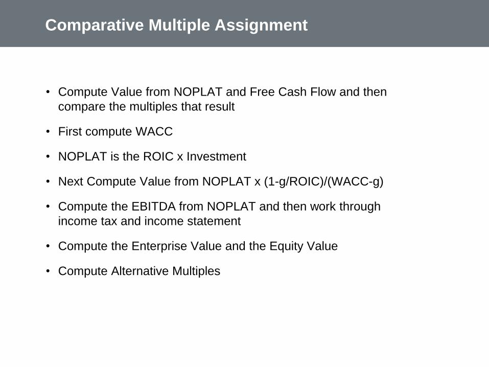
Comparative Multiple Assignment
• Compute Value from NOPLAT and Free Cash Flow and then
compare the multiples that result
• First compute WACC
• NOPLAT is the ROIC x Investment
• Next Compute Value from NOPLAT x (1-g/ROIC)/(WACC-g)
• Compute the EBITDA from NOPLAT and then work through
income tax and income statement
• Compute the Enterprise Value and the Equity Value
• Compute Alternative Multiples

First, Find the File

Work through the formulas
• Compute WACC
• Compute NOPLAT
• NOPLAT = EBIT x (1-t)
• This Means EBIT = NOPLAT/(1-t)
• EBITDA = EBIT + Depreciation Expense
• Depreciation Expense = Investment x Depreciation Rate
• Debt = Investment x Debt Percent
• Interest Expense = Debt x Interest Rate

Data Table with Multiples

P/E Ratio, Growth and Required Return
• P/E = (1/r) + PVGO/EPS
PVGO -- present value per share of future growth
opportunities
r -- required rate of return on equity
• This formula does not include the component of whether
earnings are greater than cost of capital

Industry by Industry P/E Analysis
• High P/E companies have relatively low ROE, where ROE is expected to increase.
• Computer Hardware and Recreational Products have high P/E and high ROE –
expect a lot of economic profit and treadmill
• Low P/E companies have low and growth such as utility companies or high ROE
that cannot be maintained such as tobacco companies

Industry by Industry P/E Ratio – Sorted from Highest to Lowest

Industry by Industry P/E Ratio – Sorted from Highest to Lowest
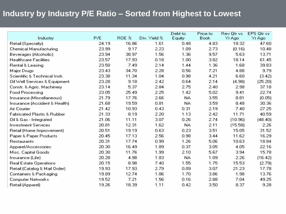
Industry by Industry P/E Ratio – Sorted from Highest to Lowest

Industry by Industry P/E Ratio – Sorted from Highest to Lowest

Finance Professor
• A finance professor received a call from a large financial institution in New York, asking him to
interview for a position on their scientific advisory committee. He agreed to go up and interview,
knowing that such a position would be prestigious and with the extra income we would be able to
purchase more consumer durables. As all of you know, interviews are a long and painful process.
The interviews lasted two days and at the end of the last day the professor was interviewing with
the chief executive who would ultimately be making the hiring decision. At the very end of the
interview, the executive asked him, “what is 7 times 3?” The finance professor confidently
responded, “22.”
• When he got home from New York his family, for once, was eagerly awaiting his return… with lists
of consumer durables in their hands. “How did it go?” they asked. “Good,” he said, “except in the
last interview they asked me 7x3 and I said 22.” “Ohh! Dad!!!” they cried, “it’s 21!” They threw out
their lists of consumer durables, knowing he would never get the job.
• Much to his surprise he got a call 2 weeks later saying he’d gotten the position and the firm was
having a reception in his honor. At the reception he found the executive and went up to him. “Do
you remember our interview?” the professor asked. “Yes,” said the executive. “And do you
remember when you asked me 7x3 and I said 22.” “Yes,” replied the executive, “I wrote down
your answer.” “Well the correct answer is 21,” said the professor, “why did I get the job?” “Well,”
said the executive, “of all the finance professors we interviewed… you were the closest.”
• The moral of the story is, if I can do this, you can do this: pricing bonds and non-American options
using monte carlo simulation to replicate the results achieved explicitly using decision trees.
Finance Professors
• A medical doctor, an engineer, and a finance professor are at a cocktail
party.
The medical doctor pompously asserts that the medical profession is
the oldest profession. He cites a passage from the Bible, in Genesis
where god creates man and woman. “Surely,” he says, “this was the
first medical act.”
The engineer jumps in and says, “I remember a passage prior to
that, which says, out of the chaos and confusion, God created the
earth. Surely, this was the first act of engineering and predates the
first medical act.”
“Aha!” says the finance professor, “who created the confusion?!”
• Condolences regarding the confusing nature of risk management under
non-uniformly shifting yield curve conditions followed.
Related Documents