2009:142 CIV MASTER'S THESIS Inverse Kinematics1018821/FULLTEXT01.pdf · This chapter introduces the fundamental principles of kinematics and how for-ward and inverse kinematics are

2009:142 CIV

M A S T E R ' S T H E S I S

Inverse Kinematics

Rickard Nilsson

Luleå University of Technology

MSc Programmes in Engineering Computer Science and Engineering

Department of Computer Science and Electrical EngineeringDivision of Computer Science

2009:142 CIV - ISSN: 1402-1617 - ISRN: LTU-EX--09/142--SE

Preface

The work for this thesis was conducted under the fall of 2007 at Agency9 ABin Lule̊a for Lule̊a University of technology - Computer Sciene and Engineering.Agency9 wanted an evaluation for some of the most used methods that can solveinverse kinematics.

I would like to thank all the guys at the office, Tomas, Khashayar, Thomas,Lasse, Johan, Martin and Richard at Agency9 in Lule̊a, who have listened andanswered many questions.

1

Abstract

The computer is getting more powerful every day and creating animations for a3D model ”on the fly” rather than pre-made animations is getting more feasible.A 3D model that is composed by segments and joints, formed for example likea human, can also be viewed as a kinematic model, the joints can be modifiedsuch that different postures can be achieved for the model. A kinematic modelhave a hierarchic tree structure with a parent-child relationship. A change madeto a parent propagates to its children. Interacting with a kinematic model canbe done in two distinct ways, forward kinematics and inverse kinematics.

The most common way of interacting with a kinematic model is by usingforward kinematics, which works by changing each joint until a desirable postureis achieved. The other way, known as inverse kinematics is more complex andneeds more computer resources, only need a direction or a position for any jointof where it should be.

The inverse kinematic methods are all using a matrix called Jacobian matrix,which consists of all first-order partial derivates derived from a kinematic model.

The main goal of this thesis is to evaluate current methods solving InverseKinematics and to see if it possible to create animations ”on the fly” for a model.

Contents

1 Introduction 31.1 Agency9 and AgentFX . . . . . . . . . . . . . . . . . . . . . . . . 31.2 Problem formulation . . . . . . . . . . . . . . . . . . . . . . . . . 41.3 Delimitations . . . . . . . . . . . . . . . . . . . . . . . . . . . . . 4

2 Theory 52.1 Kinematics . . . . . . . . . . . . . . . . . . . . . . . . . . . . . . 5

2.1.1 Degree of Freedom . . . . . . . . . . . . . . . . . . . . . . 62.1.2 Constraints . . . . . . . . . . . . . . . . . . . . . . . . . . 6

2.2 Forward Kinematics . . . . . . . . . . . . . . . . . . . . . . . . . 62.3 Inverse Kinematics . . . . . . . . . . . . . . . . . . . . . . . . . . 7

2.3.1 Analytical Solver . . . . . . . . . . . . . . . . . . . . . . . 82.3.2 Iterative Solver . . . . . . . . . . . . . . . . . . . . . . . . 92.3.3 Creating the Jacobian . . . . . . . . . . . . . . . . . . . . 102.3.4 Using the Jacobian . . . . . . . . . . . . . . . . . . . . . . 11

2.4 Solvers of inverse kinematics . . . . . . . . . . . . . . . . . . . . . 122.4.1 Transpose . . . . . . . . . . . . . . . . . . . . . . . . . . . 132.4.2 Pseudoinverse . . . . . . . . . . . . . . . . . . . . . . . . . 132.4.3 Damped Least Squares . . . . . . . . . . . . . . . . . . . . 152.4.4 Singular Value Decomposition . . . . . . . . . . . . . . . . 162.4.5 Full and Half Jacobian . . . . . . . . . . . . . . . . . . . . 17

2.5 Scene Graph . . . . . . . . . . . . . . . . . . . . . . . . . . . . . 17

3 Implementation 193.1 COLLADA . . . . . . . . . . . . . . . . . . . . . . . . . . . . . . 19

3.1.1 COLLADA Libraries . . . . . . . . . . . . . . . . . . . . . 203.1.2 Animation Library . . . . . . . . . . . . . . . . . . . . . . 203.1.3 Visual Scene Library . . . . . . . . . . . . . . . . . . . . . 21

3.2 COLLADA and IK . . . . . . . . . . . . . . . . . . . . . . . . . . 213.3 Deriving the Jacobian . . . . . . . . . . . . . . . . . . . . . . . . 223.4 Mathematic Tools . . . . . . . . . . . . . . . . . . . . . . . . . . 233.5 Animation . . . . . . . . . . . . . . . . . . . . . . . . . . . . . . . 23

1

CONTENTS CONTENTS

4 Evaluation 244.1 Constants . . . . . . . . . . . . . . . . . . . . . . . . . . . . . . . 24

4.1.1 Transpose . . . . . . . . . . . . . . . . . . . . . . . . . . . 244.1.2 Modified Transpose . . . . . . . . . . . . . . . . . . . . . 244.1.3 Damped Least Square . . . . . . . . . . . . . . . . . . . . 254.1.4 Pseudoinverse with null space . . . . . . . . . . . . . . . . 254.1.5 Constants linear relationship . . . . . . . . . . . . . . . . 25

4.2 Models . . . . . . . . . . . . . . . . . . . . . . . . . . . . . . . . . 254.3 Tests . . . . . . . . . . . . . . . . . . . . . . . . . . . . . . . . . . 264.4 Summary . . . . . . . . . . . . . . . . . . . . . . . . . . . . . . . 29

5 Conclusions 315.1 Future work . . . . . . . . . . . . . . . . . . . . . . . . . . . . . . 32

Bibliography 34

2

Chapter 1

Introduction

The performance of a computer is increasing every year and game producers havethe ability to use it more extensively, not only for plain graphic improvementsbut also for other algorithms. Algorithms for creating animations ”on the fly”that look natural for an animal or human with the ability to freely interact withthe surrounding environment is hard to do with current animation techniques.Currently, most animations are pre-generated with few possibilities of beeingable to alter it. Special problems arises when there are dynamical changes inthe enivronment. For instance if there is a pre made animation of a human armreaching a door knob, the animation has to be made in consideration of exactlywhere the objects are positioned. If the door shrunk to half its size or just weremoved further away the given animation would not change it self accordingly.

To compensate for the dynamical changes in the environment a diffrent ap-proach is needed. Given a human arm model, which consists of a segments andjoints connected to each other. By calculating the angular scalars for each jointsuch that the palm of the hand is as close it can get to the door knob wouldcompensate for moving the door knob. This method is called Inverse Kinemat-ics (IK) and it is a way of making articulated models, for example a humanor an animal model, to move more freely within its boundaries and be able tointeract in a very different manner.

1.1 Agency9 and AgentFX

Agency9 AB1 was founded in 2003 with the vision to ”make high-performancethree dimensional visualization, 3D, available to everone and everywhere”. Atthat time an advanced platform for real-time rendering of 3D graphics calledAgentFX had been developed. AgentFX is basically a platform-independet 3Dengine written in Java using OpenGL, which also supports loading the open

1www.agency9.se

3

1.2. PROBLEM FORMULATION CHAPTER 1. INTRODUCTION

schema for digital-asset, known as COLLADA (see section 3.1), for creatingscene-graphs. The AgentFX engine is tightly connected to the COLLADA-structure [14].

1.2 Problem formulation

There are two distinct methods of solving inverse kinematics, analytical anditerative. The iterative method gives the solution by solving an approximationof the system, and by updating the system with the output from the solver eachiteration until it converges. The analytical method solves the whole system atonce.

The major part of this thesis will examine and evaluate several methods ofsolving inverse kinematics for articulated models and the possibility to use ittogether with AgentFX. It will mainly be focused on iterative methods, but alsogive a short survey of the analytical approach.

An other large part of this thesis will be to create a scene-graph-like structurefor the IK and to understand the properties of a scene-graph, such as howtransformations of rotation and translation works with inverse kinematics.

The final implemented solution must be general and dynamic in regard tothe variety of models it shall be able to handle. A major problem to consideris that the system has to be robust since it’s known that some methods thatsolves inverse kinematics becomes instable in some situations. The instabilitywill be reflected in the articulated model as fast and undesirable movements.

The system also has to be fast enough such that slower computers will beable to handle the algorithm, which can be very complex.

Another important thing to point out is that the inverse kinematic applica-tion shall not be integrated within the AgentFX 3D-engine, it should only havethe ability to control it.

1.3 Delimitations

Since the IK solution shall not be integrated within the AgentFX 3D-engine ithas to have its own tree structure much like a scene graph with node properties astranslation and rotation transformations. Content created by the IK applicationcan never be stored in a COLLADA file since it is not defined in its standard.

As the algorithms of inverse kinematics are rather complex in nature, onlya few algorithms using the Jacobian matrix will be implemented and tested.

4

Chapter 2

Theory

This chapter introduces the fundamental principles of kinematics and how for-ward and inverse kinematics are defined. Further will it present different meth-ods for solving inverse kinematics.

2.1 Kinematics

Kinematics is defined as ”study of motion: a branch of physics that deals withthe motion of system without reference to force and mass” [1]. A kinematicmodel is built with segments and joints in a hierarchic structure with a parent-child relationship.

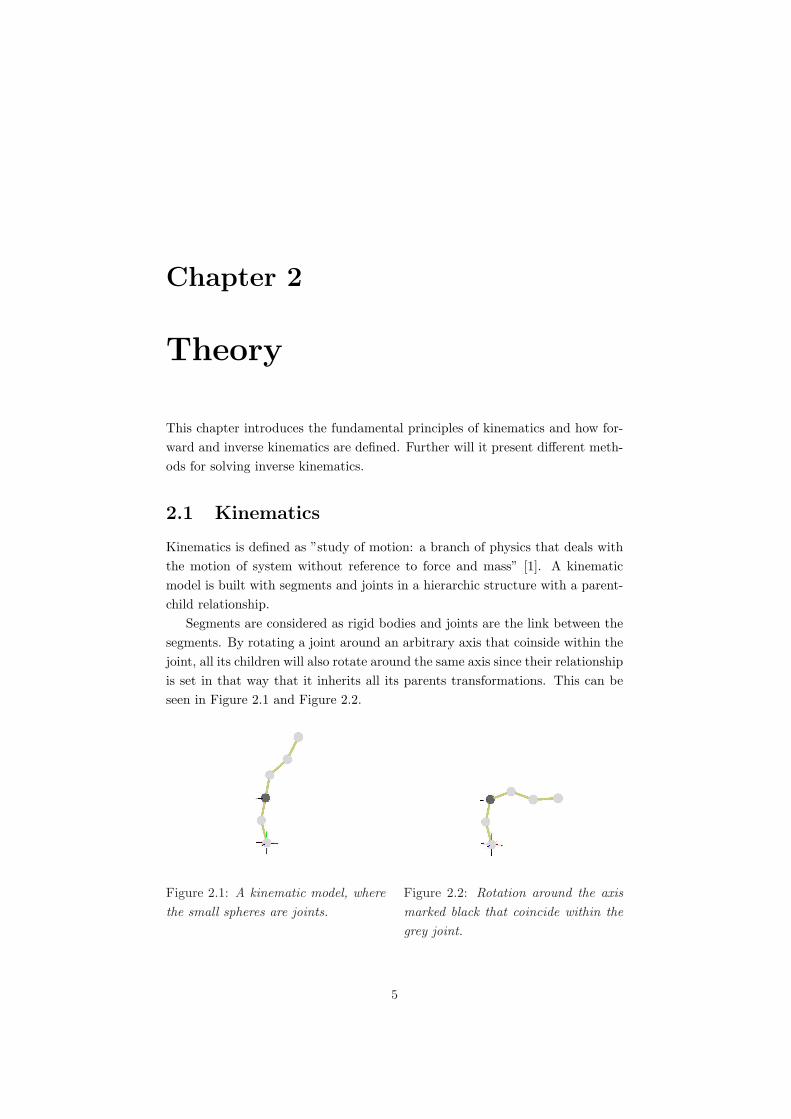
Segments are considered as rigid bodies and joints are the link between thesegments. By rotating a joint around an arbitrary axis that coinside within thejoint, all its children will also rotate around the same axis since their relationshipis set in that way that it inherits all its parents transformations. This can beseen in Figure 2.1 and Figure 2.2.

Figure 2.1: A kinematic model, wherethe small spheres are joints.

Figure 2.2: Rotation around the axismarked black that coincide within thegrey joint.

5

2.2. FORWARD KINEMATICS CHAPTER 2. THEORY

Joints can be given the ability to rotate and translate, if a joint can rotatearound one axis it is said to have one degree of freedom. The same is fortranslations.

2.1.1 Degree of Freedom

The number of degrees of freedom a joint can have is directly related to howmany dimensions the joint is in. In three dimensions the joint can have at mostthree rotational and three transitional degrees of freedom, where the rotationaland transitional axises are orthogonal sets.

In short the degree of freedom explains how a joint can move in their space.Typcial joints in three dimensions are: hinge, pivot, universal and ball joints.

Hinge and pivot joints have one degree of freedom, pivot joints are restrictedto rotate along an axis towards its child. Universal joints are based on two hingejoints with 90 degree displacement of eachother, which means that it can bendin any direction. The ball joint have three degrees of freedom and works likethe universal joint with the addition that it can rotate along an axis towards itschild.

Transitional joints are easier to define since they can only move along a givenaxis. That is with one degree of freedom it can move along a line, with two itcan move in a plane and with three it will be able to move in a room.

For simplicity regarding notation this thesis will only handle rotational jointbut the theory works for transitional joints aswell. The orientation of a rota-tional joint is decided by real scalars that is in the case of rotational joints theangle of a joint.

2.1.2 Constraints

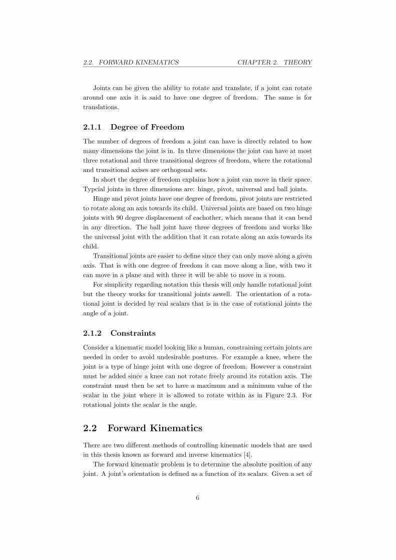
Consider a kinematic model looking like a human, constraining certain joints areneeded in order to avoid undesirable postures. For example a knee, where thejoint is a type of hinge joint with one degree of freedom. However a constraintmust be added since a knee can not rotate freely around its rotation axis. Theconstraint must then be set to have a maximum and a minimum value of thescalar in the joint where it is allowed to rotate within as in Figure 2.3. Forrotational joints the scalar is the angle.

2.2 Forward Kinematics

There are two different methods of controlling kinematic models that are usedin this thesis known as forward and inverse kinematics [4].

The forward kinematic problem is to determine the absolute position of anyjoint. A joint’s orientation is defined as a function of its scalars. Given a set of

6

2.3. INVERSE KINEMATICS CHAPTER 2. THEORY

Figure 2.3: A constraint has been set to the joint

rigid bodies linked with joints, the posture of this kinematic model is specifiedby the orientation of the joints. The absolute position of a specific joint, calledend effector, can then be determine as a function of the joint scalars θ = θ1, ..., θn

p = f (θ) (A-1)

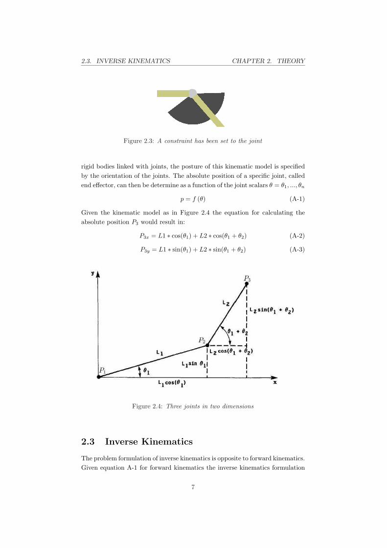
Given the kinematic model as in Figure 2.4 the equation for calculating theabsolute position P3 would result in:

P3x = L1 ∗ cos(θ1) + L2 ∗ cos(θ1 + θ2) (A-2)

P3y = L1 ∗ sin(θ1) + L2 ∗ sin(θ1 + θ2) (A-3)

Figure 2.4: Three joints in two dimensions

2.3 Inverse Kinematics

The problem formulation of inverse kinematics is opposite to forward kinematics.Given equation A-1 for forward kinematics the inverse kinematics formulation

7


can be seen as: ”Given an absolute position for an end effector, is there aconfiguration for the joints such that the end effector is positioned at the givenabsolute position?”. This means from the equation A-1 a new equation can bederived as:

θ = f−1(p) (A-4)

There are two distinct methods for solving the equation A-4, one is to ana-lytically solve the equation and the other is to solve it iteratively, which meansthat a simplified version of the equation are calculated and evaluated repeatedlyover time. Analytical solutions are precise but the complexity of it arises whenlarge chains of joints are tried to be solved [5]. Using iterative methods goodappoximations are computed with the use of the Jacobian matrix.

2.3.1 Analytical Solver

Analytical sovlers will produce all possible solutions that satisfy the given inversekinematic problem.

If a model have enough of degrees of freedom for it to cover its workspacethere is usually a finite number of solutions. If there are too few degrees offreedom there are no solutions, and if there are too many there are an infinitenumber of solutions. In the case of no solutions the solver would not returnvalues that can be used for positioning the model. For example, there is noreal solution to θ = arccos(x

l ), where x > l. The analytical solvers basicallycorresponds to solving n equations with n unknows, which also is the actualproblem using the analytical solvers.

The following is an example of solving an inverse kinematic problem usingan analytical method that is placed in two dimensions. Consider a two segmentchain as in Figure 2.4. Here P denotes a joint with a degree of freedom of one,θ the angular scalars and L the length of the segment. The relative positions ofP can be written as a vector:

P2 = [L1 cos(θ1), L1 sin(θ1)] (A-5)

P3 = [L2 cos(θ1 + θ2), L1 sin(θ1 + θ2)] (A-6)

The absolute position of P3 can by found by adding A-5 with A-6 and amore readable form can be derived:

P3x = [L1 cos(θ1) + L2 cos(θ1 + θ2)] (A-7)

P3y = [L1 sin(θ1) + L2 sin(θ1 + θ2)] (A-8)

8


This can be expanded to

P3x = (L1 + L2 cos(θ2)) cos(θ1)− L2 sin(θ2) sin(θ1) (A-9)

P3y = (L1 + L2 cos(θ2)) sin(θ1)− L2 sin(θ2) cos(θ1) (A-10)

By using trigonometric formulas the equations A-9 and A-10 can be solved givenan absolute positon to P3, θ2 and θ1 will then be found as follows:

cos(θ2) =(P 2

3x + P 23y)− (L2

1 + L22)

2L1L2(A-11)

tan(θ1) =−L2 sin(θ2)P3x + (L1 + L2 cos(θ2))P3y

L2 sin(θ2)P3y + (L1 + L2 cos(θ2))P3x(A-12)

To this specific problem there are two solutions,θ2, θ1 and −θ2, θ1 +2α, thisexample is also mention in [5].

Since these equations of these systems are in forms of sines and cosines theycan be solved systematically. However a general solution for large chains ofsegments and joints is not feasible, because the complexity of the intermediateterms grows fast when variables are eliminated.

The positive effect of analytically solvers are the precise scalars they give asoutput, once a solution is reached, joints can be altered and the end effectorwill reach its goal with a single calulation. A downside is that when thereare many solutions it is hard to know which solutions that are good. A goodsolution includes how the joints are positioned, and on graphical models thejoints should be positioned in natural way.

2.3.2 Iterative Solver

The iterative methods uses the Jacobian matrix which is a linear approximationof a differentiable function near a given point. Similar to the analytical solverthere is a function for each joint that describes instead of their relative position,the movement of the end effector. However, since both of these functions arenon linear, a linear approximation is derived from the relative position such thatit describes a partial movement of the end effector. From these approximationsa Jacobian matrix can be created.

J(θ) =∂f

∂θ(A-13)

Each column of J describes an approximated change of the end effectorsposition when changing the corresponding joint scalar. By multiplying the Ja-cobian matrix with a set of scalars ∆θ which describes the a change of eachscalar in the configuration, an approximate change ∆P of the position of theend effector will be resolved.

9


∆P = J(θ)∆θ (A-14)

Equation A-14 results in an estimated change of the end effector which issimilar to the forward kinematic problem seen in equation A-1. The differencebetween them is that equation A-14 is a linear approximation and easier toresolve. An approximate change of the scalars ∆θ can be resolved by invertingthe function J(θ). The equation A-14 can then be written as:

∆θ = J(θ)−1∆P (A-15)

This means in other words, given an articulated structure with a set of n

scalars θ and an end effector P , a Jacobian matrix can be created by usingequation A-13. By inverting the Jacobian, approximated scalars ∆θ can beresolved with equation A-15.

Since the Jacobian matrix is created by linear approximations, the result∆θ from equation A-15 are also approximations of the change in the jointscalars. This leads to an iterative method since equation A-15 gives approx-imated changes in θ the equation needs to be done repeatedly. Let ∆P be~e = t − P , where t is the target position, P is the end effector position and~e is the desirable change of the end effector. The first iteration will result ina θ from equation A-13 and equation A-15 which are added to the articulatedmodel joint scalars. By using forward kinematics a new position P of the endeffector is acquired and a new iteration begins. This is done until either ~e issmall enough or the end effector does not move.

2.3.3 Creating the Jacobian

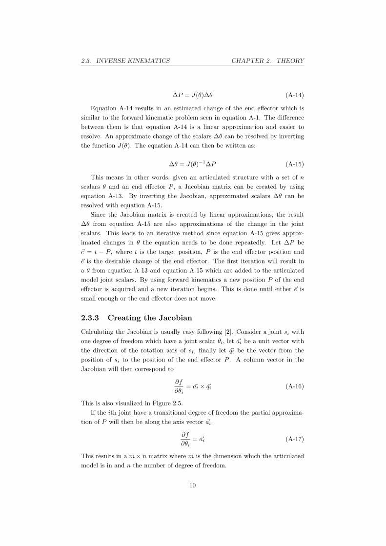
Calculating the Jacobian is usually easy following [2]. Consider a joint si withone degree of freedom which have a joint scalar θi, let ~ai be a unit vector withthe direction of the rotation axis of si, finally let ~qi be the vector from theposition of si to the position of the end effector P . A column vector in theJacobian will then correspond to

∂f

∂θi= ~ai × ~qi (A-16)

This is also visualized in Figure 2.5.If the ith joint have a transitional degree of freedom the partial approxima-

tion of P will then be along the axis vector ~ai.

∂f

∂θi= ~ai (A-17)

This results in a m× n matrix where m is the dimension which the articulatedmodel is in and n the number of degree of freedom.

10


Figure 2.5: A graphical kinematic model. The black joint marked P is the endeffector, the lines point out from it are the partial derivates from equation A-16.

There is also a more complex version of the Jacobian where m = l×k, wherel is the dimension and k the number of end effectors involved in the Jacobianwhich also will be discussed later in this thesis.

2.3.4 Using the Jacobian

All methods for solving inverse kinematics that are discussed in this thesis areusing the Jacobian matrix as its basis.

There are two ways of using the Jacobian matrix to solve inverse kinematics.One is to use the transpose of the Jacobian JT [7, 8]. The other is to calculate theinverse of the Jacobian J−1, which is actually needed following the equation A-15.

Inverting the Jacobian matrix is not trivial, following the section 2.3.3 itturns out that the jacobian is non square if the degree of freedom is greaterthan the dimension the model is in. Alternative methods for inverting theJacobian is then needed. Methods of solving J−1 are discussed in [2, 10, 6] andsome methods will be discussed with more depth in this thesis.

11

2.4. SOLVERS OF INVERSE KINEMATICS CHAPTER 2. THEORY

2.4 Solvers of inverse kinematics

There are several methods of solving inverse kinematics with the Jacobian,transpose methods [7, 8], pseudoinverse methods [4], Damped Least Squaresmethod [9], Kim and Buss’ Selectively Damped Least Squares method [3, 2].Most of these methods are also mentioned and explained in [2].

Unreachable targets are also discussed in some of the papers. Some of themethods suffers from jerky movments when the end effector is trying to track aposition that is out of range. In section 2.4.3 one way of tracking a position ispresented. Another way to reduce this is by clamping the range to the targetpositions introduced in [3]. What they do is to instead of just setting ~e as thedesirable change, a method reduces ~e if it is too large.

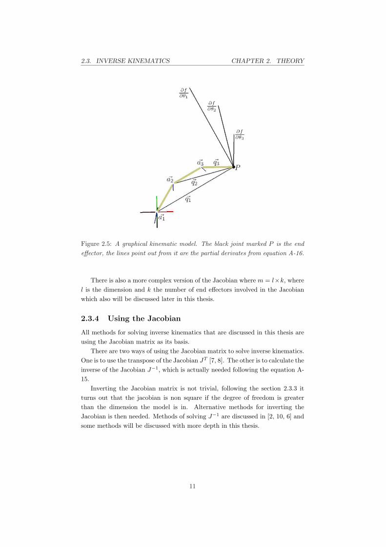
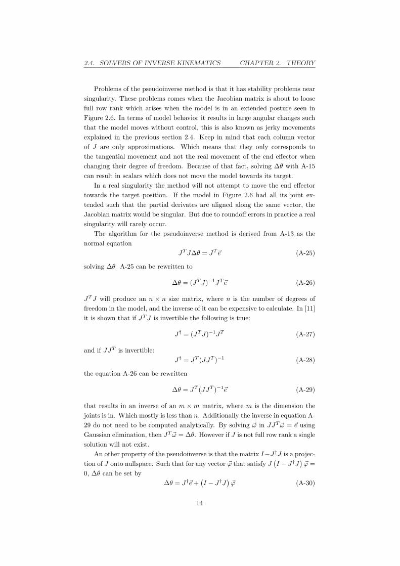
Jerky movements is a result of large irregular changes of the scalars θ. Theselarge changes comes when the Jacobian matrix is about to loose full row rankand when the target position is out of range. In other words when the model asin Figure 2.6 is almost fully extended, the partial derivates are all almost alongthe same line (two dimensions) or plane (three dimensions). Solving equation A-15 or in other words constructing ~e from the partial derivates will then resultin large scalars, therefore the jerky movements.

Figure 2.6: A graphical kinematic model in an almost exended posture.

Joint constraints is not a part of the Jacobian matrix, instead once a changein the angular scalar is received, the constraint decide whether it is possible tochange the angle. When an articulated model has a large number of constraintsit will then make the solver slower to reach its target position.

12


2.4.1 Transpose

This method have been used for inverse kinematics among other by [7]. Themethod uses the transpose of the Jacobian matrix instead of the inverse. It hasbeen proven in [2] that it is possible to justify the use of it, simplified they saythat the dot product of ∂f

∂θi

Tand ~e will result in a scalar that have the correct

sign but the magnitude is of wrong size. This method resolves the equation A-15to

∆θ = αJT~e (A-18)

for some scalar α. A way of choosing α is also presented in that paper. Theyuse the relationship between the desired change ~e and an approximated changeof the end effector which is defined as JJT~e. By assuming that JJT~e is the realchange, α is chosen such that it is as close as possible to ~e:

α =< ~e, JJT~e >

< JJT~e, JJT~e >(A-19)

This method is according to [3] fast to calculate since it do not need any solvingof inverses.

2.4.2 Pseudoinverse

The pseudoinverse method is used to solve equation A-15. It is used becauseJ is most likely redundant and non square, thus an ordinary inverse is notpossible. The resulting scalars are used for rotating the joints degrees of freedom.Pseudoinverse is also called Moore-Penrose inverse. This method sets ∆θ equalto

∆θ = J†~e (A-20)

where J† is the pseudoinverse of J . J† is defined for matrices in [11]. Propertiesof J† which are also shared with normal inverses are:

JJ†J = J (A-21)

J†JJ† = J† (A-22)(J†J

)∗= J†J (A-23)

(JJ†

)∗= JJ†. (A-24)

Where ∗ is the conjugate transpose, if J contains all real values J∗ is equal toJT . Note that J†J is a symmetric square matrix also known as Hermitian.

In [2] they state that using the pseudoinverse will give the best solution tothe equation J∆θ = ~e in the sense of least squares. If ~e is in the column spanof J , ∆θ is an unique vector of smallest magnitude satisfying A-13. If ~e isnot in the column span an exact value of ∆θ is impossible to get, however ∆θ

minimizes the magnitude difference of J∆θ − ~e.

13


Problems of the pseudoinverse method is that it has stability problems nearsingularity. These problems comes when the Jacobian matrix is about to loosefull row rank which arises when the model is in an extended posture seen inFigure 2.6. In terms of model behavior it results in large angular changes suchthat the model moves without control, this is also known as jerky movementsexplained in the previous section 2.4. Keep in mind that each column vectorof J are only approximations. Which means that they only corresponds tothe tangential movement and not the real movement of the end effector whenchanging their degree of freedom. Because of that fact, solving ∆θ with A-15can result in scalars which does not move the model towards its target.

In a real singularity the method will not attempt to move the end effectortowards the target position. If the model in Figure 2.6 had all its joint ex-tended such that the partial derivates are aligned along the same vector, theJacobian matrix would be singular. But due to roundoff errors in practice a realsingularity will rarely occur.

The algorithm for the pseudoinverse method is derived from A-13 as thenormal equation

JT J∆θ = JT~e (A-25)

solving ∆θ A-25 can be rewritten to

∆θ = (JT J)−1JT~e (A-26)

JT J will produce an n × n size matrix, where n is the number of degrees offreedom in the model, and the inverse of it can be expensive to calculate. In [11]it is shown that if JT J is invertible the following is true:

J† = (JT J)−1JT (A-27)

and if JJT is invertible:J† = JT (JJT )−1 (A-28)

the equation A-26 can be rewritten

∆θ = JT (JJT )−1~e (A-29)

that results in an inverse of an m × m matrix, where m is the dimension thejoints is in. Which mostly is less than n. Additionally the inverse in equation A-29 do not need to be computed analytically. By solving ~ω in JJT ~ω = ~e usingGaussian elimination, then JT ~ω = ∆θ. However if J is not full row rank a singlesolution will not exist.

An other property of the pseudoinverse is that the matrix I−J†J is a projec-tion of J onto nullspace. Such that for any vector ~ϕ that satisfy J

(I − J†J

)~ϕ =

0, ∆θ can be set by∆θ = J†~e +

(I − J†J

)~ϕ (A-30)

14


In this manner ∆θ will still result in a value that minimizes J∆θ−~e. In [4] thenullspace is used to determine the error of the calculated pseudoinverese.

Error = ||(I − JJ†)~e|| (A-31)

Since JJ†~e gives an approximated change of the end effector, hence equation A-31 will give a magnitude error of the desired change. If the error is too large, ~e

is reduced to half it length.

2.4.3 Damped Least Squares

Using the damped least squares is a way of removing and reducing near singu-larites in the Jacobian matrix and stabilizing ∆θ. This method is also calledLevenberg-Marquardt algorithm and one of the first to use it was Wampler [9].In equation A-14 the search for a minimum vector ∆θ that gives the best solu-tion was wanted. In this method, ∆θ that minimizes

||J∆θ − ~e||2 − λ2||∆θ||2 (A-32)

where λ is a non zero real value constant. Equation A-32 can be rewritten as∣∣∣∣∣

∣∣∣∣∣

(JT

λI

)∆θ −

(~e

0

)∣∣∣∣∣

∣∣∣∣∣ (A-33)

such that the normal equation A-25 resolves to(

J

λI

)T (J

λI

)∆θ =

(J

λI

)T (~e

0

)(A-34)

Following the steps in equation A-27, A-28 and A-29 the solution to ∆θ willlook like

∆θ = JT (JJT + λ2I)−1~e (A-35)

What this means is that by adding the orthonormal set I it is guaranteed that aninverse exists, however choosing λ too small will still result in jerky movments,when the model is in an extended posture, which is the same problem as withthe pseudoinverse method. This means in mathematical terms that by lettingλ in equation A-35 approach zero it results in equation A-29. If λ is too large,the scalars ∆θ will become smaller such that each iteration will only change theend effector position very little and the number of needed iteration to reach thegoal would grow.

The constant λ must be chosen such that neither of the above becomes aproblem. It is suggested that the constant depends on details of the articulatedmodel, but there is no mention of selecting the constant directly in [2], howeverit have some references to a number of authors that proposes a way of selectingit dynamically.

15


A more practical way of explaining this method is by using Figure 2.6 wherethe model is in an extended posture and its corresponding Jacobian matrix isin near singular. Solving the Jacobian would normally result in large scalarsand in its turn a jerky model behaviour. By adding two vectors orthogonalto each other, along x-axis and along y-axis, in the Jacobian matrix, solving ~e

becomes easier and would result in smaller scalars. The constant λ determineshow long the two vectors are, and by choosing a large λ the two vectors relievesthe scalars from resulting in large values.

2.4.4 Singular Value Decomposition

Singular value decomposition is not a method in it self, but it can however beused to calculate and analyze the pseudoinverse of the Jacobian. It is used by [3]to optimize the damped least squares method to their selectively damped leastsquares method.

It is stated in [10] that if J is an m × n matrix with row rank r it can bedecomposed to

J = UEV T (A-36)

where U is a m ×m, E a m × n and V a n × n matrix. E contains diagonalentires of the r first singular values of J ,σi = ei,i,σ1 ≥ σ2 ≥ . . . ≥ σr. U and V

are orthogonal matrices. Where U forms an orthonormal basis for <m and V

for <n which also is known as the nullspace of J . The pseudoinverse of J withSVD is defined by

J† = V E†UT (A-37)

Since E contains a diagonal r × r matrix D, E is formed like

E =

(D

000

)(A-38)

and the pseudoinverse

E† =

(D†

000

). (A-39)

The inverse of D is defined by

d†i,i =

{1/di,i ifdi,i 6= 00 ifdi,i = 0

(A-40)

It is also common to write A-36 as a sum of vectors

J =m∑

i=1

σiuivTi =

r∑

i=1

σiuivTi (A-41)

then the pseudoinverse is equal to

J =r∑

i=1

1σi

viuTi (A-42)

16

2.5. SCENE GRAPH CHAPTER 2. THEORY

The properties that can be exploited in SVD lies withing the matrix E and itssingular values which have been used by [3].

2.4.5 Full and Half Jacobian

In [4] they introduce the concept of full and half jacobian, where half means po-sitioning and full positioning and orientation. In case of positioning the desiredchange ~e only consider the position, ~e = [∆x, ∆y, ∆z] while the full also includethe current orientation of the end effector, such that ~e is a vector containing sixelements. The full Jacobian adds additional information to each entry, the firstthree rows contains the partial derivates from each degree of freedom, the lastthree contains information of the rotation axises of the degrees of freedom.

2.5 Scene Graph

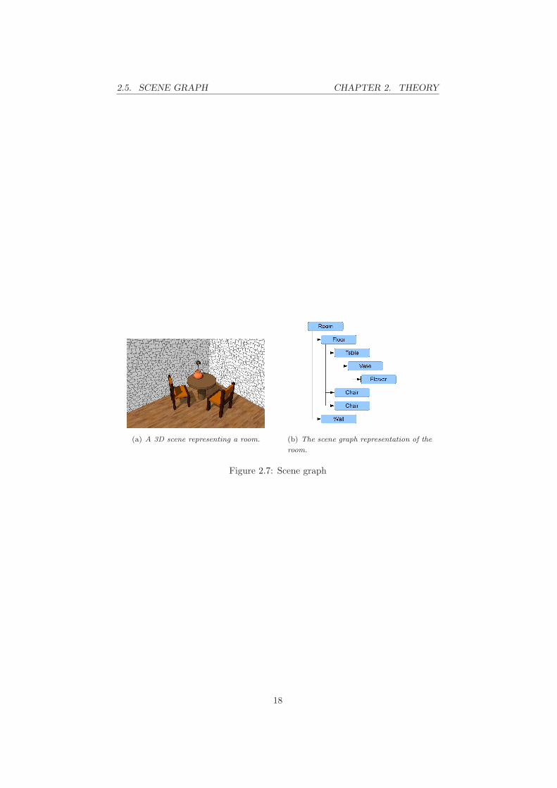
A scene graph is a structure which is often used to arrange the logical andspatial representation of a graphical scene. There is not a clear definition ofa scene graph since programmers who implement them generally only use thebasic principles to create structure suiting the application [14].

The basic principles of a scene graph is a collection of nodes arranged intoa graph or tree structure. This indirectly implies that a node may have manychildren but seldom more than a single parent. If an operation is applied to anode the effect propagates to all its members. In many cases such operationconsists of a transformation matrix which is associated with the node. Thematrices are easy to concatenate and it can be done efficently when the operationpropagates down to its children [13].

The transformation matrix associated with a node is generally a 4×4 matrixformed by concatenating one or several geometrical transformation matriceswhich can among other describe rotations, translations and scaling. In otherwords the transformation matrix describes the location and orientation of anode’s coordinate system relative to its parent.

17

2.5. SCENE GRAPH CHAPTER 2. THEORY

(a) A 3D scene representing a room. (b) The scene graph representation of the

room.

Figure 2.7: Scene graph

18

Chapter 3

Implementation

3.1 COLLADA

COLLADA1 is short term for COLLAborative Design Activity which definesan extensible markup language (XML) scheme that enables free exchanges ofdigital assets for 3D-applications without loss of information. COLLADA wasinitiated by Sony computer entertainment to create a standard for digital as-sets and a goal to liberate it from proprietary binary formats and was furtherdeveloped by the Khronos group2 in 2006. The Khronos group was founded in2000 by leading media centric companies, including 3Dlabs, NVIDIA, SGI, SunMicrosystems, Intel, ATI, SGI and Discreet. The group is dedicated to createopen standards to a variety of devices and platforms.

There were several goals and guidelines for the COLLADA digital assetschema when it was created [12]. One of them ”To liberate digital assets fromproprietary binary formats into a well-specified, XML-bases, open-source for-mat”. This goal was set because a large part of a 3D-application is definedby digital assets. Investments on proprietary binary formats are considerablylarge, and even after these investments it only gives the developer the ability toexport and import the format, not a possibility to modify the data outside thetool and import it later.

This goal led into a few decisions regarding the format of COLLADA, in-cluding:

• It will use XML. XML provides a well defined standard that deals withissues such as character sets, and parsers for almost all languages andplatforms already exists.

• No binary data will reside within the COLLADA file. Since many lan-1http://www.collada.org/2http://www.khronos.org/

19

3.1. COLLADA CHAPTER 3. IMPLEMENTATION

guages do not easily support binary data within XML and in general theydo not have support for manipulation, so by having no binary data it sim-plifies it. COLLADA does however provide means to reference an externalbinary file.

These decisions lead to a COLLADA document with some rules. A COL-LADA document contains a mandatory header element, while libraries and a setof scenes are optional, which all are set under the root element <COLLADA>.The header element is tagged with <asset> and containts basic informationabout COLLADA-version used, author and other information that the devel-oper consider as individual assets.

3.1.1 COLLADA Libraries

A COLLADA document is built from a sequence of organized libraries of specifictypes. A library describes some part of a scene, for example an animation. Thelibraries that are used in this thesis are the animation library and the visualscene library.

3.1.2 Animation Library

The animation library contains a set of one or more animation elements. Eachanimation element basically describes a transformation of an object or valueover a specified time period, most commonly to give a model the illusion ofmotion. A form of animation is the simple key-frame animation where a key-frame contains a value that is linked with a key. Given a set of these key-framesan animation can be derived. In other words, given a model and a set of key-frames, where the keys are time indexes and the linked values are positions of amodels arm, an interpolated postion of the model’s arm can be calculated givenany specified time within the key-frames [12].

To make the previous possible a COLLADA-animation consist of three el-ments: a source, a sampler and a channel element. The source element <source>is a reference to a one dimensional array that can be accessed. In order to cre-ate a key-frame two sources are needed, one ”input” where the time indexesare stored and one ”output” that will contain values corresponding to the timeindexes. Interpolation type can also be set in the source element, other elementswithin this have information including length of the array and stride. The stridetells the sampler element how many of the values belongs together.

The <sampler> element is used as an intermediator to sort out what valuesin the source element that is input and output and to create n-dimensionalarrays from the values.

The <channel> element connects the output values to the object that shallbe transformed. It has two mandatory elements: a reference to a source and

20

3.2. COLLADA AND IK CHAPTER 3. IMPLEMENTATION

a target. In this case the source would be the output from the sampler, andtarget is the object.

3.1.3 Visual Scene Library

The visual scene library contains a set of one or more visual scene elements. Avisual scene element describes visual aspects of a COLLADA document. Theelement forms a root of an organized hierarchic structure formed like a tree datastructure, also known as a scene graph, of <node> elements that contains visualinformation and related data.

The <node> element has five optional attributes:

• id - A text string containing the unique identifier of the element. Thisvalue must be unique within the instance document.

• name - The text string name of the element.

• sid - A text string value containing the subidentifier of this element. Thisvalue must be unique within the scope of the parent element.

• type - The type of the <node> element. Valid values are JOINT or NODE.The default is ”NODE”.

• layer - The names of the layers to which this node belongs.

The type attribute is the main attribute that will be used within this thesis.If that attribute is set to the value JOINT it means the node is part of anarticulated structure for example a kinematic model.

A node can also contain instances of cameras, controllers, geometries andlights where the instances are defined in their respective library. They can alsocontain other nodes which is seen as children. Nodes defines their own localcoordinate system which is relative to their parent. Their relative coordinatesystem is decided by any number of three dimensional tranformations. COL-LADA defines six transformation elements that may be used within these nodes:lookat, matrix, rotate, scale, skew and translate, where all can be transformedinto a 4×4 matrix for accumulation. By altering the transformations a desirableposition or orientation can be attained.

3.2 COLLADA and IK

COLLADA version 1.4 does not have a specific implementation of inverse kine-matics and since AgentFX is tightly connected to the COLLADA-structure, itwas not an option to fully integrate this application within AgentFX. However,using attributes set by the standard it is possible to retreive information from

21

3.3. DERIVING THE JACOBIAN CHAPTER 3. IMPLEMENTATION

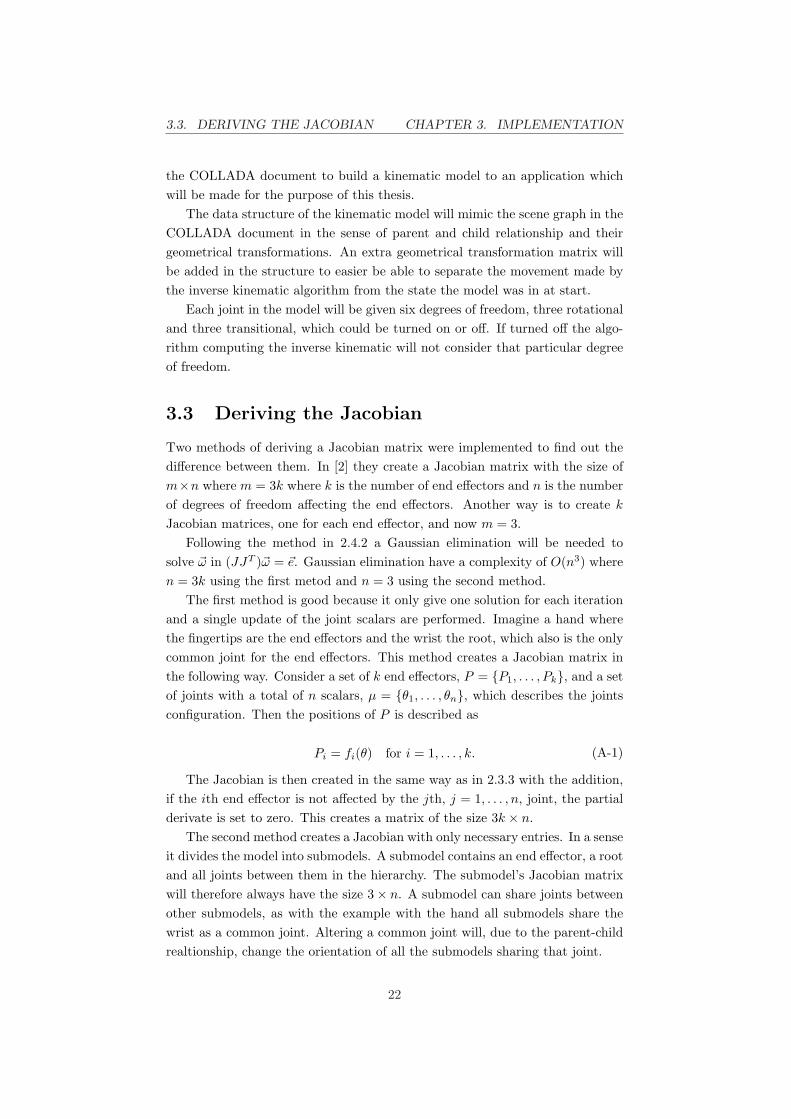
the COLLADA document to build a kinematic model to an application whichwill be made for the purpose of this thesis.

The data structure of the kinematic model will mimic the scene graph in theCOLLADA document in the sense of parent and child relationship and theirgeometrical transformations. An extra geometrical transformation matrix willbe added in the structure to easier be able to separate the movement made bythe inverse kinematic algorithm from the state the model was in at start.

Each joint in the model will be given six degrees of freedom, three rotationaland three transitional, which could be turned on or off. If turned off the algo-rithm computing the inverse kinematic will not consider that particular degreeof freedom.

3.3 Deriving the Jacobian

Two methods of deriving a Jacobian matrix were implemented to find out thedifference between them. In [2] they create a Jacobian matrix with the size ofm×n where m = 3k where k is the number of end effectors and n is the numberof degrees of freedom affecting the end effectors. Another way is to create k

Jacobian matrices, one for each end effector, and now m = 3.Following the method in 2.4.2 a Gaussian elimination will be needed to

solve ~ω in (JJT )~ω = ~e. Gaussian elimination have a complexity of O(n3) wheren = 3k using the first metod and n = 3 using the second method.

The first method is good because it only give one solution for each iterationand a single update of the joint scalars are performed. Imagine a hand wherethe fingertips are the end effectors and the wrist the root, which also is the onlycommon joint for the end effectors. This method creates a Jacobian matrix inthe following way. Consider a set of k end effectors, P = {P1, . . . , Pk}, and a setof joints with a total of n scalars, µ = {θ1, . . . , θn}, which describes the jointsconfiguration. Then the positions of P is described as

Pi = fi(θ) for i = 1, . . . , k. (A-1)

The Jacobian is then created in the same way as in 2.3.3 with the addition,if the ith end effector is not affected by the jth, j = 1, . . . , n, joint, the partialderivate is set to zero. This creates a matrix of the size 3k × n.

The second method creates a Jacobian with only necessary entries. In a senseit divides the model into submodels. A submodel contains an end effector, a rootand all joints between them in the hierarchy. The submodel’s Jacobian matrixwill therefore always have the size 3× n. A submodel can share joints betweenother submodels, as with the example with the hand all submodels share thewrist as a common joint. Altering a common joint will, due to the parent-childrealtionship, change the orientation of all the submodels sharing that joint.

22

3.4. MATHEMATIC TOOLS CHAPTER 3. IMPLEMENTATION

Each iteration consists of creating the Jacobian, solving the Jacobian andfinally update the submodel’s joints with the given changes, this will be donefor all submodels. A side effect is that it will result in multiple updates on allcommon joints in each iteration when the model have multiple end effectors. Inother words, given the same hand as above there are five submodels, one foreach fingertip. A Jacobian matrix would first be created with the first fingeras an end effector and the wrist as a root. Then by solving the first matrix,by any mentioned method, a set of joint scalars can then be applied to thecorresponding joints. This step will be repeated for all submodels. By usingthis method the wrist joint itself would be changed five times each iteration.In a really bad scenario the first submodel could for instance change the wrist90◦ and the second submodel change it back 90◦, this results in that the firstchange to the shared joint would be more or less gone. In addition to that, thefirst submodel’s end effector would be further off its target than it was beforedue to the parent-child relationship.

3.4 Mathematic Tools

Several tools were needed to be able to compute a scene graph and calcula-tions related to the creation of the Jacobian matrix. Most of the mathematicmethods involving linear algebra and computing 3D content was found withinAgentFX that were ready to use. However a method for solving Ax = b usingGaussian elimination was needed, as mention in a previous chapter a part ofthe pseudoinverse do not need the inverse that is seen in the methods.

3.5 Animation

AgentFX provides the means of loading and saving a COLLADA document.By loading the document it creates a scene graph where it is possible to modifyand add extra content. The content that this application shall be able to addis animation information. A method that adds a key-frame for all joints thatcould be called upon was needed.

23

Chapter 4

Evaluation

The following methods were tested to solve inverse kinematics: transpose, modi-fied transpose, pseudoinverse, pseudoinverse with null space control and dampedleast squares.

4.1 Constants

The constants chosen in the methods are described below. The dampeningconstant λ for the damped least squares method were not present in any of thereferenced papers. Because of this a small study of the behavior for the dampedleast squares method were used to determine a balanced dampening constantwhich considered the current state of the articulated model at each iteration.

The resulting column vector ∆θ from all the methods were multiplied witha scalar set to 10, otherwise the articulated model converged to the targetpositions too slowly.

The following section describes how the constants were chosen in their method.The pure pseudoinverse method did not have any constants to be set.

4.1.1 Transpose

The constant α was chosen in the same way as described in [2]

4.1.2 Modified Transpose

The difference in this modifed transpose method is a dampening factor muchlike the one described in damped least squares, which is added into the Jacobianmatrix in order to stabilize when tracking targets out of range. The constantα was chosen like in the transpose method. The dampening factor was setdynamically as the magnitude of the desirable change added with the magnitudeof the distance between the end effector and the root.

24

4.2. MODELS CHAPTER 4. EVALUATION

4.1.3 Damped Least Square

The dampening constant λ was chosen as the magnitude of the desirable changeof the end effector added with a small constant which was set at each iteration.The small constant was in this case 1/100 of the total sum of the segments fromroot to end effector. The magnitude of the desirable change is a nice value of λ

since it more or less ensures that the Jacobian matrix does not get near singularat any time. The small constant were added because when the target positionswere nearly out of range, it started oscillating since the desirable change wastoo small to dampen.

As seen in Figure 2.6 an orthogonal set of vectors where each vector has thelength of the desirable change vector ~e will damp effciently. This will howeveralso reduce the speed when setting target positions that are in range but farfrom the end effector.

4.1.4 Pseudoinverse with null space

This method was derived from [4] and is also explained in the pseudoinversechapter. The maximum error was set to 1.

4.1.5 Constants linear relationship

Since some constant values in the methods were chosen and set at each iterationit was vital to see if they had a linear relationship. In order to determine if theyare correctly chosen the model and the target positions were resized with ascalar. By first comparing the number of iterations by the first model andpaths with the resized model, they should remain the same. It turned out thatthe constants were chosen with a linear relationship, resizing the model and thetarget positions with the same scalar did not affect the number of iterations.

4.2 Models

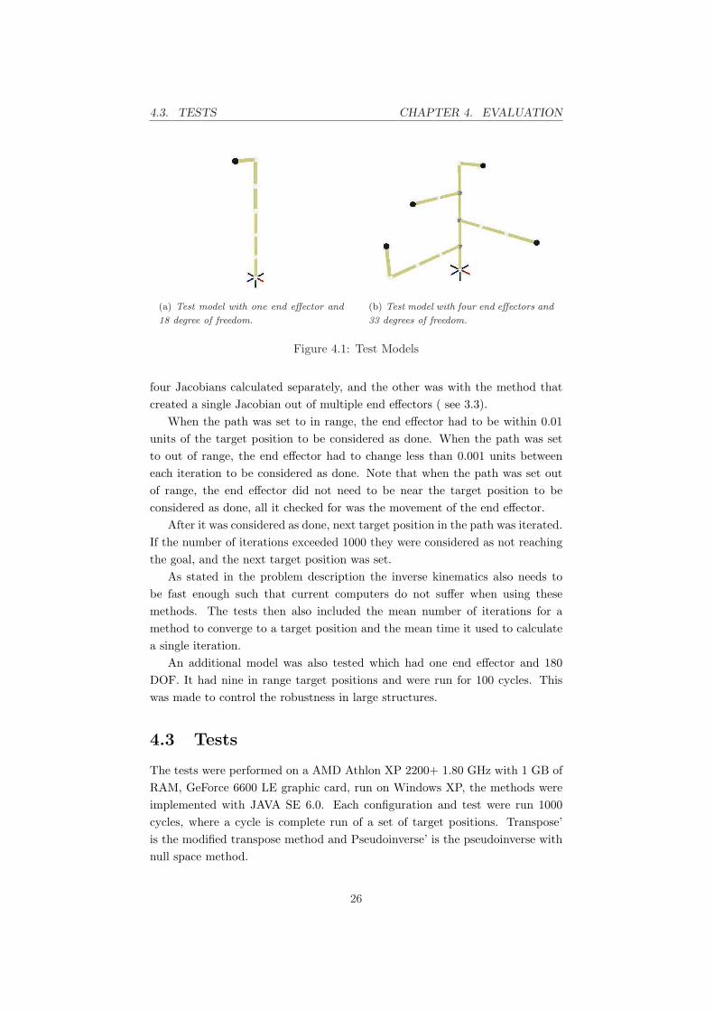
There were two different models that were used, one model had a single endeffector and 18 degrees of freedom Figure 4.1(a) and a model with four endeffectors and a total of 33 degrees of freedom Figure 4.1(b). Additionally amodel with 180 degrees of freedom were also used to determine if the methodswere stable in a large chain. The range between each joint was set to 1 unit.

From the problem description two different tests were derived from eachconfiguration to test the robustness. One test the target positions were inrange for the end effector, the other test the targets where out of range. Thetarget positions (path) for the single arm had nine targets and the multiplearm configuration had four target positions. The second configuration withfour end effectors were tested with two different methods, the first was with

25

4.3. TESTS CHAPTER 4. EVALUATION

(a) Test model with one end effector and

18 degree of freedom.

(b) Test model with four end effectors and

33 degrees of freedom.

Figure 4.1: Test Models

four Jacobians calculated separately, and the other was with the method thatcreated a single Jacobian out of multiple end effectors ( see 3.3).

When the path was set to in range, the end effector had to be within 0.01units of the target position to be considered as done. When the path was setto out of range, the end effector had to change less than 0.001 units betweeneach iteration to be considered as done. Note that when the path was set outof range, the end effector did not need to be near the target position to beconsidered as done, all it checked for was the movement of the end effector.

After it was considered as done, next target position in the path was iterated.If the number of iterations exceeded 1000 they were considered as not reachingthe goal, and the next target position was set.

As stated in the problem description the inverse kinematics also needs tobe fast enough such that current computers do not suffer when using thesemethods. The tests then also included the mean number of iterations for amethod to converge to a target position and the mean time it used to calculatea single iteration.

An additional model was also tested which had one end effector and 180DOF. It had nine in range target positions and were run for 100 cycles. Thiswas made to control the robustness in large structures.

4.3 Tests

The tests were performed on a AMD Athlon XP 2200+ 1.80 GHz with 1 GB ofRAM, GeForce 6600 LE graphic card, run on Windows XP, the methods wereimplemented with JAVA SE 6.0. Each configuration and test were run 1000cycles, where a cycle is complete run of a set of target positions. Transpose’is the modified transpose method and Pseudoinverse’ is the pseudoinverse withnull space method.

26


The column ”time for one iteration” in the presented tables is the total timeit takes to create Jacobian, calculating ∆θ and updating the inverse kinematicstree structure. Creating Jacobian and the update are the same for all methods,however the total time is of interest when there is a need to find out how manyof these iterations can be done within each update of the graphical environment.

Method Mean iterations Time for one iteration

Pseudoinverse 32 96.4 µsPseudoinverse’ 46 104.1 µs

DLS 35 89.2 µsTranspose 59 83.3 µsTranspose’ 163 84.8 µs

Table 4.1: Model with one end effector, 18 DOF, target positions in range

Table 4.1 shows that the Pseudoinverse method have the least number ofiterations, the time for one iteration is a bit higher due to the use of an an-alytical inverse of the Jacobian matrix, while the DLS are solving with rowreduction. However Pseudoinverse’ needs an analytical inverse to calculate theerror magnitude, its even higher calculation time comes from the control of theerror.


Pseudoinverse - - µsPseudoinverse’ - - µs

DLS 74 81.5 µsTranspose 117 73.8 µsTranspose’ 98 77.8 µs

Table 4.2: Model with one end effector, 18 DOF, target positions out of range

Table 4.2 shows that both pseudoinverse methods could not produce anyresult when target positions were out of range. The pure pseudoinverse methodgets unstable (see 2.4.2) and the joint scalars got out of hand. On the otherhand the pseudoinverse’ did not get unstable, instead the error control and insome degree the implementation of it made this method unable to move oncereaching for the first target position was done. When the next target positionshould be reached for the end effector did not move more than 0.001 units andthe method thought it was done.

Table 4.3 shows when having a model with 180 DOF the pure pseudoin-verse method got a bit unstable after a few cycles and the number of iterationsincreased in comparison to DLS.

27



Pseudoinverse 59 684 µsPseudoinverse’ 343 715 µs

DLS 45 593 µsTranspose 130 580 µsTranspose’ 153 586 µs

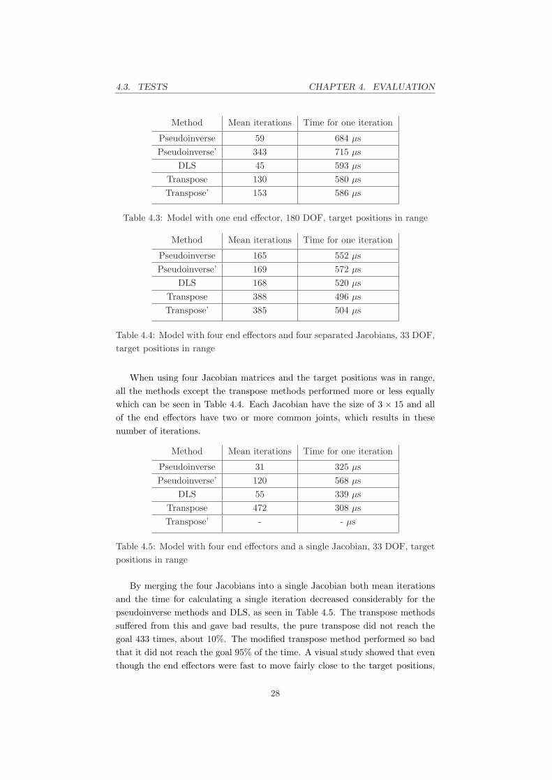
Table 4.3: Model with one end effector, 180 DOF, target positions in range




Table 4.4: Model with four end effectors and four separated Jacobians, 33 DOF,target positions in range

When using four Jacobian matrices and the target positions was in range,all the methods except the transpose methods performed more or less equallywhich can be seen in Table 4.4. Each Jacobian have the size of 3 × 15 and allof the end effectors have two or more common joints, which results in thesenumber of iterations.



DLS 55 339 µsTranspose 472 308 µsTranspose’ - - µs

Table 4.5: Model with four end effectors and a single Jacobian, 33 DOF, targetpositions in range

By merging the four Jacobians into a single Jacobian both mean iterationsand the time for calculating a single iteration decreased considerably for thepseudoinverse methods and DLS, as seen in Table 4.5. The transpose methodssuffered from this and gave bad results, the pure transpose did not reach thegoal 433 times, about 10%. The modified transpose method performed so badthat it did not reach the goal 95% of the time. A visual study showed that eventhough the end effectors were fast to move fairly close to the target positions,

28

4.4. SUMMARY CHAPTER 4. EVALUATION

they converged too slow to achieve the goal within 1000 iteration.



DLS 390 476 µsTranspose - - µsTranspose’ 350 452 µs

Table 4.6: Model with four end effectors and four separated Jacobians, 33 DOF,target positions is out of range

Table 4.6 shows that the out of range test when using four Jacobians alsohad the same effect as the single out of range test with the pseudoinverse meth-ods. The pure transpose method oscillated when a visual study was made toinvestigate the loss of results. The DLS method was stable and the modifiedtranspose method converged to its target the fastest.




Table 4.7: Model with four end effectors and a single Jacobian, 33 DOF, targetpositions is out of range

Table 4.7 shows that the pure Transpose method was fast when using thesingle Jacobian. The Transpose’ method in this case there were 28 times themethod could not solve within 1000 iterations.

4.4 Summary

The only method to produce results in all the tests in the previous sectionwere the Damped Least Squares method, this due to the dampening factor thateffectively stabilizes the resulting joint scalars when the target positions wereout of range. The Damped Least Squares method is also a fairly fast methodand is often placed right after the fastest method when counting the number ofiterations.

The Pseudoinverse method reaches the target positions with the least num-ber of iterations when they were in range. But when the target positions are out

29

4.4. SUMMARY CHAPTER 4. EVALUATION

of range, the lack of a dampening factor causes the Jacobian matrix to get nearsingular and the resulting joint scalars became too large such that the modelstarted to move irradically.

The Pseudoinverse method which were using null space to try stabilize thejoint scalars when target positions were out of range needed most time for eachiteration. This method did not produce any results when the target positionswere out of range which part can be blamed on the implementation and theother part can be blamed on the method it self.

The transpose method produced results in all tests except when it used fourJacobians and the targets were out of range. The modified transpose methodonly outperformed the other methods when using multiple Jacobians with multi-ple end effectors. When using a merged single Jacobian the number of iterationsand time generally decreased.

30

Chapter 5

Conclusions

This thesis has presented test-results of how different methods of inverse kine-matics perform in various situations in order to determine if they are suitable tobe used in real-time applications. An application for testing the methods werealso built.

If I were to use any method to solve the inverse kinematic problem I woulduse the damped least square method. Looking at the results it can handle bothtarget positions that are in range and out of range without generating any jerkymovement to the model. One problem with the damped least square method isthe way I chose the constant λ. Since the constant depends on the length of thedesired change, the farther away the target position was compared to the endeffector the slower the method would converge. In [2] they explain that a way ofremoving this side effect is to clamp the desired change. Given a model withouttransitional joints it can move at most two times the total length of the model(the sum of all segment lengths from the end effector to the root. Clamping thedesirable change to that length will result in a faster method when the distancefrom the end effector to the target position are farther than the total length ofthe model.

The transpose method is supposed to be a fast algorithm according to [3].However, looking at the results, there is nothing that indicates that. I tried tomake it faster by increasing the scalars output with a larger constant but it onlymade it more instable.

My attempt to make the transpose method more stable worked in the casewhere there were several Jacobian matrices involved and the result surprisedme, but with the single Jacobian it was a bad choice.

Is it then possible to use this to create an animation by directing the endeffectors and take key frames in real time? The answer is yes, given the currentcomputers it is possible. Lets say that you have a 3D game that would give theinverese kinematic method 10 ms to iterate a solution each frame, which means

31

5.1. FUTURE WORK CHAPTER 5. CONCLUSIONS

that the game would be able to reach up to 100 frames per second. If the modelhad the configuration with the multiple end effectors, and the same computerthese methods were tested on. The computer can iterate about 29 times. Byusing the DLS method, half the number of iterations can be accomplished inthat time needed for the model to reach its target when the target position isin range. But since an animation rarely moves from one posture into anotherinstantly, it is not a problem that the model only made it half way.

Due to the lack of literature explaining how constraints should be handled ina way where the inverese kinematic methods don’t give results that can exceedthe constraints. What you would want is a method that doesn’t give resultsthat can exceed the working limits of the joint. Therefore, any documentedtests for handling constraints were never done in this thesis. However, in [6] avery simple way of implementing constraints are presented, which checks all thejoints after each iteration. If a joint has exceeded any of the constraints it forcesthe joint back into a position were the constraints have not been surpassed.This also means that the restrictions are never considered when creating theJacobian matrix, all joints are treated equal. Play with the idea of a modelthat had a constraint set to have a working limit of zero, such as it basically isnot a degree of freedom. The creation of the Jacobian matrix will however notrecognize this, and treat this as any other joint. The solvers themselves doesn’teither recognize constraints, they only return a summary of all changes of thejoints that should move the end effector to its target. By having a joint thatexceeded its constraint would then remove a part of that summary and movethe end effector less close to the target. Using the simple way of dealing withconstraints results in a chance of reducing the effectiveness of the solvers whendealing with a model that have any number of constraints.

5.1 Future work

There is a lot of future work on this subject and the implementation of thekinematic tree structure could be optimized. Reading [13] I saw that there canbe a lot of improvement of the kinematic scene graph that is currently used. Asit is now mainly 4×4 transformation matrices are used within the nodes. Theseare geometrical transformation matrices and they inherit some features that canbe used to reduce the complexity of multiplying two matrices. I strongly believethat my implementation of the kinematic scene graph could be improved suchthat it only would need half the time it needs now to update its data structure.

Although this thesis did not cover much of how to constrain joints, I did playwith the idea of how to improve the method mentioned in [6]. One way of im-proving it would be by removing a joint’s degree of freedom once it has exeededits constraint, this would result in a Jacobian matrix that does not consider that

32

5.1. FUTURE WORK CHAPTER 5. CONCLUSIONS

specific degree of freedom. Solving it with any of the methods results in scalarsthat would be more correct and they would not loose effectiveness when morejoints exceeds its constraint. However it is hard to know when a joint’s degreeof freedom have returned into its working limits.

An other idea I had is to add a priority scalar, ϕ, ranging from 0 to 1 infrontof the partial derivate, ϕ ∂f

∂θi. If a degree of freedom tries to exceed its limit

the priority would be reduced. This means that the partial derivate becomessmaller and the inverse kinematic method returns a smaller scalar change inthat specific DOF. Once it makes a change back into its constraint the priorityresets to normal.

33

Bibliography

[1] Encarta Dictionary, ”http://encarta.msn.com”, 2009

[2] Samuel R. Buss, ”Introduction to Inverse Kinematics with JacobianTranspose, Pseudoinverse and Damped Least Squares Methods”, April 17,2004 Unpublished

[3] Samuel R. Buss and Jin-Su Kim, ”Selectively Damped Least Squares forInverse Kinemetaics”, 2004

[4] Michael Meredith and Steve Maddoc, ”Real-Time Inverse Kinematics:The Return of the Jacobian”

[5] BertHold K. P. Horn, ”Kinematics, Statics and Dynamics of Two-dimensional Manipulators” in Artifical Inteliigence: An MIT PerspectiveVol. 2, Winston, P.H. and R.H. Brown (Eds.), pp. 273-310, MIT Press

[6] Kang Teresa Ge, ”Solving Inverse Kinematics constraint Problems forHighly Articulated Models”,2000

[7] W.A Wolovich and H. Elliot, ”A Computational Technique For InverseKinematics”, 1984

[8] Daniel E. Whitney, ”Resolved Motion Rate Control of Manipulatros andHuman Prostheses”; 1969

[9] Charles W. Wampler, ”Manipulator Inverse Kinematics Solutions Basedon Vector Formulations and Damped Least-Squares Methods”, 1986

34

BIBLIOGRAPHY BIBLIOGRAPHY

[10] David C. Lay, ”Linear algebra and its applications” second edition, 2000

[11] Lennard R̊ade and Bertil Westergren, ”Mathematics Handbook for Scienceand Engineering”, 1989, 1998 fourth edition

[12] COLLADA - Digital Asset Schema Release 1.4.1 (2006).http://www.khronos.org/¯les/collada spec 1 4.pdf

[13] David H. Eberly, ”3D Game Engine Design”, 1999

[14] Johan Lindberg, ”Implementation of a COLLADA scene-graph”, 2006

35

2009:142 CIV MASTER'S THESIS Inverse Kinematics1018821/FULLTEXT01.pdf · This chapter introduces the fundamental principles of kinematics and how for-ward and inverse kinematics are

Documents