A Practical Guide to Geostatistical Mapping Tomislav Hengl

2009 a Practical Guide to Geostatistical Mapping
Oct 28, 2015
Welcome message from author
This document is posted to help you gain knowledge. Please leave a comment to let me know what you think about it! Share it to your friends and learn new things together.
Transcript

A Practical Guide to Geostatistical Mapping
Tomislav Hengl
Hen
gl, T
.A
Pra
ctic
al
Gu
ide
to
Ge
ost
ati
stic
al
Ma
pp
ing
http://spatial-analyst.net/book/
Printed copies of this book can be ordered via
www.lulu.com
178440 181560
178440 181560
333760
329600
178440 181560
178440 181560
333760
329640
333760
329640
ordinary kriging
4.72
7.51
40% 70%universal kriging
333760
329600
Geostatistical mapping can be defined as analytical production of maps by using field
observations, auxiliary information and a computer program that calculates values at
locations of interest. The purpose of this guide is to assist you in producing quality maps by
using fully-operational open source software packages. It will first introduce you to the
basic principles of geostatistical mapping and regression-kriging, as the key prediction
technique, then it will guide you through software tools – R+gstat/geoR, SAGA GIS and
Google Earth – which will be used to prepare the data, run analysis and make final layouts.
Geostatistical mapping is further illustrated using seven diverse case studies: interpolation
of soil parameters, heavy metal concentrations, global soil organic carbon, species density
distribution, distribution of landforms, density of DEM-derived streams, and spatio-
temporal interpolation of land surface temperatures. Unlike other books from the “use R”
series, or purely GIS user manuals, this book specifically aims at bridging the gaps between
statistical and geographical computing. Materials presented in this book have been used for the five-day advanced training course
“GEOSTAT: spatio-temporal data analysis with R+SAGA+Google Earth”, that is periodically
organized by the author and collaborators.
Visit the book's homepage to obtain a copy of the data sets and scripts used in the exercises:
Fig. 5.19. Mapping uncertainty for zinc visualized using whitening: ordinary kriging (left) and universal kriging (right). Predicted values in log-scale.
Get involved: join the R-sig-geo mailing list!

1

1
The methods used in this book were developed in the context of the EcoGRID and LifeWatch projects. ECOGRID (analysis2
and visualization tools for the Dutch Flora and Fauna database) is a national project managed by the Dutch data authority3
on Nature (Gegevensautoriteit Natuur) and financed by the Dutch ministry of Agriculture (LNV). LIFEWATCH (e-Science and4
Technology Infrastructure for Biodiversity Research) is a European Strategy Forum on Research Infrastructures (ESFRI)5
project, and is partially funded by the European Commission within the 7th Framework Programme under number 211372.6
The role of the ESFRI is to support a coherent approach to policy-making on research infrastructures in Europe, and to act7
as an incubator for international negotiations about concrete initiatives.8
This is the second, extended edition of the EUR 22904 EN Scientific and Technical Research series report published by9
Office for Official Publications of the European Communities, Luxembourg (ISBN: 978-92-79-06904-8).10
Legal Notice:11
12
Neither the University of Amsterdam nor any person acting on behalf of the University of Amsterdam is re-13
sponsible for the use which might be made of this publication.14
15
Contact information:16
17
Mailing Address: UvA B2.34, Nieuwe Achtergracht 166, 1018 WV Amsterdam18
Tel.: +31- 020-525737919
Fax: +31- 020-525745120
E-mail: [email protected]
http://home.medewerker.uva.nl/t.hengl/22
23
ISBN 978-90-9024981-024
25
This document was prepared using the LATEX 2ε software.26
Printed copies of this book can be ordered via http://www.lulu.com27
28
© 2009 Tomislav Hengl29
30
31
32
The content in this book is licensed under a Creative Commons Attribution-Noncommercial-No Derivative Works3.0 license. This means that you are free to copy, distribute and transmit the work, as long as you attributethe work in the manner specified by the author. You may not use this work for commercial purposes, alter,transform, or build upon this work without an agreement with the author of this book. For more information seehttp://creativecommons.org/licenses/by-nc-nd/3.0/.
33

1
“I wandered through http://www.r-project.org. To state the good I foundthere, I’ll also say what else I saw.
Having abandoned the true way, I fell into a deep sleep and awoke in a deep darkwood. I set out to escape the wood, but my path was blocked by a lion. As I fled tolower ground, a figure appeared before me. ‘Have mercy on me, whatever you are,’ Icried, ‘whether shade or living human’.”
Patrick Burns in “The R inferno”
2


A Practical Guide to 1
Geostatistical Mapping 2
by Tomislav Hengl 3
November 2009 4


Contents 1
1 Geostatistical mapping 1 2
1.1 Basic concepts . . . . . . . . . . . . . . . . . . . . . . . . . . . . . . . . . . . . . . . . . . . . . . . . . . . 1 3
1.1.1 Environmental variables . . . . . . . . . . . . . . . . . . . . . . . . . . . . . . . . . . . . . . . . 4 4
1.1.2 Aspects and sources of spatial variability . . . . . . . . . . . . . . . . . . . . . . . . . . . . . . 5 5
1.1.3 Spatial prediction models . . . . . . . . . . . . . . . . . . . . . . . . . . . . . . . . . . . . . . . 9 6
1.2 Mechanical spatial prediction models . . . . . . . . . . . . . . . . . . . . . . . . . . . . . . . . . . . . . 12 7
1.2.1 Inverse distance interpolation . . . . . . . . . . . . . . . . . . . . . . . . . . . . . . . . . . . . . 12 8
1.2.2 Regression on coordinates . . . . . . . . . . . . . . . . . . . . . . . . . . . . . . . . . . . . . . . 13 9
1.2.3 Splines . . . . . . . . . . . . . . . . . . . . . . . . . . . . . . . . . . . . . . . . . . . . . . . . . . . 14 10
1.3 Statistical spatial prediction models . . . . . . . . . . . . . . . . . . . . . . . . . . . . . . . . . . . . . . 14 11
1.3.1 Kriging . . . . . . . . . . . . . . . . . . . . . . . . . . . . . . . . . . . . . . . . . . . . . . . . . . . 15 12
1.3.2 Environmental correlation . . . . . . . . . . . . . . . . . . . . . . . . . . . . . . . . . . . . . . . 20 13
1.3.3 Predicting from polygon maps . . . . . . . . . . . . . . . . . . . . . . . . . . . . . . . . . . . . . 24 14
1.3.4 Hybrid models . . . . . . . . . . . . . . . . . . . . . . . . . . . . . . . . . . . . . . . . . . . . . . 24 15
1.4 Validation of spatial prediction models . . . . . . . . . . . . . . . . . . . . . . . . . . . . . . . . . . . . 25 16
2 Regression-kriging 27 17
2.1 The Best Linear Unbiased Predictor of spatial data . . . . . . . . . . . . . . . . . . . . . . . . . . . . . 27 18
2.1.1 Mathematical derivation of BLUP . . . . . . . . . . . . . . . . . . . . . . . . . . . . . . . . . . . 30 19
2.1.2 Selecting the right spatial prediction technique . . . . . . . . . . . . . . . . . . . . . . . . . . 32 20
2.1.3 The Best Combined Spatial Predictor . . . . . . . . . . . . . . . . . . . . . . . . . . . . . . . . 35 21
2.1.4 Universal kriging, kriging with external drift . . . . . . . . . . . . . . . . . . . . . . . . . . . . 36 22
2.1.5 A simple example of regression-kriging . . . . . . . . . . . . . . . . . . . . . . . . . . . . . . . 39 23
2.2 Local versus localized models . . . . . . . . . . . . . . . . . . . . . . . . . . . . . . . . . . . . . . . . . . 41 24
2.3 Spatial prediction of categorical variables . . . . . . . . . . . . . . . . . . . . . . . . . . . . . . . . . . 42 25
2.4 Geostatistical simulations . . . . . . . . . . . . . . . . . . . . . . . . . . . . . . . . . . . . . . . . . . . . 44 26
2.5 Spatio-temporal regression-kriging . . . . . . . . . . . . . . . . . . . . . . . . . . . . . . . . . . . . . . 44 27
2.6 Species Distribution Modeling using regression-kriging . . . . . . . . . . . . . . . . . . . . . . . . . . 46 28
2.7 Modeling of topography using regression-kriging . . . . . . . . . . . . . . . . . . . . . . . . . . . . . . 51 29
2.7.1 Some theoretical considerations . . . . . . . . . . . . . . . . . . . . . . . . . . . . . . . . . . . 51 30
2.7.2 Choice of auxiliary maps . . . . . . . . . . . . . . . . . . . . . . . . . . . . . . . . . . . . . . . . 53 31
2.8 Regression-kriging and sampling optimization algorithms . . . . . . . . . . . . . . . . . . . . . . . . 54 32
2.9 Fields of application . . . . . . . . . . . . . . . . . . . . . . . . . . . . . . . . . . . . . . . . . . . . . . . 55 33
2.9.1 Soil mapping applications . . . . . . . . . . . . . . . . . . . . . . . . . . . . . . . . . . . . . . . 55 34
2.9.2 Interpolation of climatic and meteorological data . . . . . . . . . . . . . . . . . . . . . . . . . 56 35
2.9.3 Species distribution modeling . . . . . . . . . . . . . . . . . . . . . . . . . . . . . . . . . . . . . 56 36
2.9.4 Downscaling environmental data . . . . . . . . . . . . . . . . . . . . . . . . . . . . . . . . . . . 58 37
iii

2.10 Final notes about regression-kriging . . . . . . . . . . . . . . . . . . . . . . . . . . . . . . . . . . . . . . 581
2.10.1 Alternatives to RK . . . . . . . . . . . . . . . . . . . . . . . . . . . . . . . . . . . . . . . . . . . . 582
2.10.2 Limitations of RK . . . . . . . . . . . . . . . . . . . . . . . . . . . . . . . . . . . . . . . . . . . . . 593
2.10.3 Beyond RK . . . . . . . . . . . . . . . . . . . . . . . . . . . . . . . . . . . . . . . . . . . . . . . . . 604
3 Software (R+GIS+GE) 635
3.1 Geographical analysis: desktop GIS . . . . . . . . . . . . . . . . . . . . . . . . . . . . . . . . . . . . . . 636
3.1.1 ILWIS . . . . . . . . . . . . . . . . . . . . . . . . . . . . . . . . . . . . . . . . . . . . . . . . . . . . 637
3.1.2 SAGA . . . . . . . . . . . . . . . . . . . . . . . . . . . . . . . . . . . . . . . . . . . . . . . . . . . . 668
3.1.3 GRASS GIS . . . . . . . . . . . . . . . . . . . . . . . . . . . . . . . . . . . . . . . . . . . . . . . . 719
3.2 Statistical computing: R . . . . . . . . . . . . . . . . . . . . . . . . . . . . . . . . . . . . . . . . . . . . . 7210
3.2.1 gstat . . . . . . . . . . . . . . . . . . . . . . . . . . . . . . . . . . . . . . . . . . . . . . . . . . . . 7411
3.2.2 The stand-alone version of gstat . . . . . . . . . . . . . . . . . . . . . . . . . . . . . . . . . . . 7512
3.2.3 geoR . . . . . . . . . . . . . . . . . . . . . . . . . . . . . . . . . . . . . . . . . . . . . . . . . . . . 7713
3.2.4 Isatis . . . . . . . . . . . . . . . . . . . . . . . . . . . . . . . . . . . . . . . . . . . . . . . . . . . . 7714
3.3 Geographical visualization: Google Earth (GE) . . . . . . . . . . . . . . . . . . . . . . . . . . . . . . . 7815
3.3.1 Exporting vector maps to KML . . . . . . . . . . . . . . . . . . . . . . . . . . . . . . . . . . . . 8016
3.3.2 Exporting raster maps (images) to KML . . . . . . . . . . . . . . . . . . . . . . . . . . . . . . . 8217
3.3.3 Reading KML files to R . . . . . . . . . . . . . . . . . . . . . . . . . . . . . . . . . . . . . . . . . 8718
3.4 Summary points . . . . . . . . . . . . . . . . . . . . . . . . . . . . . . . . . . . . . . . . . . . . . . . . . . 8819
3.4.1 Strengths and limitations of geostatistical software . . . . . . . . . . . . . . . . . . . . . . . . 8820
3.4.2 Getting addicted to R . . . . . . . . . . . . . . . . . . . . . . . . . . . . . . . . . . . . . . . . . . 9021
3.4.3 Further software developments . . . . . . . . . . . . . . . . . . . . . . . . . . . . . . . . . . . . 9622
3.4.4 Towards a system for automated mapping . . . . . . . . . . . . . . . . . . . . . . . . . . . . . 9623
4 Auxiliary data sources 9924
4.1 Global data sets . . . . . . . . . . . . . . . . . . . . . . . . . . . . . . . . . . . . . . . . . . . . . . . . . . 9925
4.1.1 Obtaining data via a geo-service . . . . . . . . . . . . . . . . . . . . . . . . . . . . . . . . . . . 10226
4.1.2 Google Earth/Maps images . . . . . . . . . . . . . . . . . . . . . . . . . . . . . . . . . . . . . . 10327
4.1.3 Remotely sensed images . . . . . . . . . . . . . . . . . . . . . . . . . . . . . . . . . . . . . . . . 10628
4.2 Download and preparation of MODIS images . . . . . . . . . . . . . . . . . . . . . . . . . . . . . . . . 10829
4.3 Summary points . . . . . . . . . . . . . . . . . . . . . . . . . . . . . . . . . . . . . . . . . . . . . . . . . . 11430
5 First steps (meuse) 11731
5.1 Introduction . . . . . . . . . . . . . . . . . . . . . . . . . . . . . . . . . . . . . . . . . . . . . . . . . . . . 11732
5.2 Data import and exploration . . . . . . . . . . . . . . . . . . . . . . . . . . . . . . . . . . . . . . . . . . 11733
5.2.1 Exploratory data analysis: sampling design . . . . . . . . . . . . . . . . . . . . . . . . . . . . . 12334
5.3 Zinc concentrations . . . . . . . . . . . . . . . . . . . . . . . . . . . . . . . . . . . . . . . . . . . . . . . . 12735
5.3.1 Regression modeling . . . . . . . . . . . . . . . . . . . . . . . . . . . . . . . . . . . . . . . . . . 12736
5.3.2 Variogram modeling . . . . . . . . . . . . . . . . . . . . . . . . . . . . . . . . . . . . . . . . . . . 13037
5.3.3 Spatial prediction of Zinc . . . . . . . . . . . . . . . . . . . . . . . . . . . . . . . . . . . . . . . . 13138
5.4 Liming requirements . . . . . . . . . . . . . . . . . . . . . . . . . . . . . . . . . . . . . . . . . . . . . . . 13339
5.4.1 Fitting a GLM . . . . . . . . . . . . . . . . . . . . . . . . . . . . . . . . . . . . . . . . . . . . . . . 13340
5.4.2 Variogram fitting and final predictions . . . . . . . . . . . . . . . . . . . . . . . . . . . . . . . . 13441
5.5 Advanced exercises . . . . . . . . . . . . . . . . . . . . . . . . . . . . . . . . . . . . . . . . . . . . . . . . 13642
5.5.1 Geostatistical simulations . . . . . . . . . . . . . . . . . . . . . . . . . . . . . . . . . . . . . . . 13643
5.5.2 Spatial prediction using SAGA GIS . . . . . . . . . . . . . . . . . . . . . . . . . . . . . . . . . . 13744
5.5.3 Geostatistical analysis in geoR . . . . . . . . . . . . . . . . . . . . . . . . . . . . . . . . . . . . 14045
5.6 Visualization of generated maps . . . . . . . . . . . . . . . . . . . . . . . . . . . . . . . . . . . . . . . . 14546
5.6.1 Visualization of uncertainty . . . . . . . . . . . . . . . . . . . . . . . . . . . . . . . . . . . . . . 14547
5.6.2 Export of maps to Google Earth . . . . . . . . . . . . . . . . . . . . . . . . . . . . . . . . . . . 14848

6 Heavy metal concentrations (NGS) 153 1
6.1 Introduction . . . . . . . . . . . . . . . . . . . . . . . . . . . . . . . . . . . . . . . . . . . . . . . . . . . . 153 2
6.2 Download and preliminary exploration of data . . . . . . . . . . . . . . . . . . . . . . . . . . . . . . . 154 3
6.2.1 Point-sampled values of HMCs . . . . . . . . . . . . . . . . . . . . . . . . . . . . . . . . . . . . 154 4
6.2.2 Gridded predictors . . . . . . . . . . . . . . . . . . . . . . . . . . . . . . . . . . . . . . . . . . . . 157 5
6.3 Model fitting . . . . . . . . . . . . . . . . . . . . . . . . . . . . . . . . . . . . . . . . . . . . . . . . . . . . 160 6
6.3.1 Exploratory analysis . . . . . . . . . . . . . . . . . . . . . . . . . . . . . . . . . . . . . . . . . . . 160 7
6.3.2 Regression modeling using GLM . . . . . . . . . . . . . . . . . . . . . . . . . . . . . . . . . . . 160 8
6.3.3 Variogram modeling and kriging . . . . . . . . . . . . . . . . . . . . . . . . . . . . . . . . . . . 164 9
6.4 Automated generation of HMC maps . . . . . . . . . . . . . . . . . . . . . . . . . . . . . . . . . . . . . 166 10
6.5 Comparison of ordinary and regression-kriging . . . . . . . . . . . . . . . . . . . . . . . . . . . . . . . 168 11
7 Soil Organic Carbon (WISE_SOC) 173 12
7.1 Introduction . . . . . . . . . . . . . . . . . . . . . . . . . . . . . . . . . . . . . . . . . . . . . . . . . . . . 173 13
7.2 Loading the data . . . . . . . . . . . . . . . . . . . . . . . . . . . . . . . . . . . . . . . . . . . . . . . . . 173 14
7.2.1 Download of the world maps . . . . . . . . . . . . . . . . . . . . . . . . . . . . . . . . . . . . . 174 15
7.2.2 Reading the ISRIC WISE into R . . . . . . . . . . . . . . . . . . . . . . . . . . . . . . . . . . . . 175 16
7.3 Regression modeling . . . . . . . . . . . . . . . . . . . . . . . . . . . . . . . . . . . . . . . . . . . . . . . 179 17
7.4 Modeling spatial auto-correlation . . . . . . . . . . . . . . . . . . . . . . . . . . . . . . . . . . . . . . . 184 18
7.5 Adjusting final predictions using empirical maps . . . . . . . . . . . . . . . . . . . . . . . . . . . . . . 184 19
7.6 Summary points . . . . . . . . . . . . . . . . . . . . . . . . . . . . . . . . . . . . . . . . . . . . . . . . . . 186 20
8 Species’ occurrence records (bei) 189 21
8.1 Introduction . . . . . . . . . . . . . . . . . . . . . . . . . . . . . . . . . . . . . . . . . . . . . . . . . . . . 189 22
8.1.1 Preparation of maps . . . . . . . . . . . . . . . . . . . . . . . . . . . . . . . . . . . . . . . . . . . 189 23
8.1.2 Auxiliary maps . . . . . . . . . . . . . . . . . . . . . . . . . . . . . . . . . . . . . . . . . . . . . . 190 24
8.2 Species distribution modeling . . . . . . . . . . . . . . . . . . . . . . . . . . . . . . . . . . . . . . . . . 192 25
8.2.1 Kernel density estimation . . . . . . . . . . . . . . . . . . . . . . . . . . . . . . . . . . . . . . . . 192 26
8.2.2 Environmental Niche analysis . . . . . . . . . . . . . . . . . . . . . . . . . . . . . . . . . . . . . 196 27
8.2.3 Simulation of pseudo-absences . . . . . . . . . . . . . . . . . . . . . . . . . . . . . . . . . . . . 196 28
8.2.4 Regression analysis and variogram modeling . . . . . . . . . . . . . . . . . . . . . . . . . . . . 197 29
8.3 Final predictions: regression-kriging . . . . . . . . . . . . . . . . . . . . . . . . . . . . . . . . . . . . . 200 30
8.4 Niche analysis using MaxEnt . . . . . . . . . . . . . . . . . . . . . . . . . . . . . . . . . . . . . . . . . . 202 31
9 Geomorphological units (fishcamp) 207 32
9.1 Introduction . . . . . . . . . . . . . . . . . . . . . . . . . . . . . . . . . . . . . . . . . . . . . . . . . . . . 207 33
9.2 Data download and exploration . . . . . . . . . . . . . . . . . . . . . . . . . . . . . . . . . . . . . . . . 208 34
9.3 DEM generation . . . . . . . . . . . . . . . . . . . . . . . . . . . . . . . . . . . . . . . . . . . . . . . . . . 209 35
9.3.1 Variogram modeling . . . . . . . . . . . . . . . . . . . . . . . . . . . . . . . . . . . . . . . . . . . 209 36
9.3.2 DEM filtering . . . . . . . . . . . . . . . . . . . . . . . . . . . . . . . . . . . . . . . . . . . . . . . 210 37
9.3.3 DEM generation from contour data . . . . . . . . . . . . . . . . . . . . . . . . . . . . . . . . . 211 38
9.4 Extraction of Land Surface Parameters . . . . . . . . . . . . . . . . . . . . . . . . . . . . . . . . . . . . 212 39
9.5 Unsupervised extraction of landforms . . . . . . . . . . . . . . . . . . . . . . . . . . . . . . . . . . . . . 213 40
9.5.1 Fuzzy k-means clustering . . . . . . . . . . . . . . . . . . . . . . . . . . . . . . . . . . . . . . . . 213 41
9.5.2 Fitting variograms for different landform classes . . . . . . . . . . . . . . . . . . . . . . . . . 214 42
9.6 Spatial prediction of soil mapping units . . . . . . . . . . . . . . . . . . . . . . . . . . . . . . . . . . . 215 43
9.6.1 Multinomial logistic regression . . . . . . . . . . . . . . . . . . . . . . . . . . . . . . . . . . . . 215 44
9.6.2 Selection of training pixels . . . . . . . . . . . . . . . . . . . . . . . . . . . . . . . . . . . . . . . 215 45
9.7 Extraction of memberships . . . . . . . . . . . . . . . . . . . . . . . . . . . . . . . . . . . . . . . . . . . 218 46
10 Stream networks (baranjahill) 221 47
10.1 Introduction . . . . . . . . . . . . . . . . . . . . . . . . . . . . . . . . . . . . . . . . . . . . . . . . . . . . 221 48
10.2 Data download and import . . . . . . . . . . . . . . . . . . . . . . . . . . . . . . . . . . . . . . . . . . . 221 49
10.3 Geostatistical analysis of elevations . . . . . . . . . . . . . . . . . . . . . . . . . . . . . . . . . . . . . . 223 50
10.3.1 Variogram modelling . . . . . . . . . . . . . . . . . . . . . . . . . . . . . . . . . . . . . . . . . . 223 51
10.3.2 Geostatistical simulations . . . . . . . . . . . . . . . . . . . . . . . . . . . . . . . . . . . . . . . 225 52
10.4 Generation of stream networks . . . . . . . . . . . . . . . . . . . . . . . . . . . . . . . . . . . . . . . . . 227 53

vi
10.5 Evaluation of the propagated uncertainty . . . . . . . . . . . . . . . . . . . . . . . . . . . . . . . . . . 2291
10.6 Advanced exercises . . . . . . . . . . . . . . . . . . . . . . . . . . . . . . . . . . . . . . . . . . . . . . . . 2312
10.6.1 Objective selection of the grid cell size . . . . . . . . . . . . . . . . . . . . . . . . . . . . . . . 2313
10.6.2 Stream extraction in GRASS . . . . . . . . . . . . . . . . . . . . . . . . . . . . . . . . . . . . . 2334
10.6.3 Export of maps to GE . . . . . . . . . . . . . . . . . . . . . . . . . . . . . . . . . . . . . . . . . . 2365
11 Land surface temperature (HRtemp) 2416
11.1 Introduction . . . . . . . . . . . . . . . . . . . . . . . . . . . . . . . . . . . . . . . . . . . . . . . . . . . . 2417
11.2 Data download and preprocessing . . . . . . . . . . . . . . . . . . . . . . . . . . . . . . . . . . . . . . . 2428
11.3 Regression modeling . . . . . . . . . . . . . . . . . . . . . . . . . . . . . . . . . . . . . . . . . . . . . . . 2449
11.4 Space-time variogram estimation . . . . . . . . . . . . . . . . . . . . . . . . . . . . . . . . . . . . . . . 24810
11.5 Spatio-temporal interpolation . . . . . . . . . . . . . . . . . . . . . . . . . . . . . . . . . . . . . . . . . 24911
11.5.1 A single 3D location . . . . . . . . . . . . . . . . . . . . . . . . . . . . . . . . . . . . . . . . . . . 24912
11.5.2 Time-slices . . . . . . . . . . . . . . . . . . . . . . . . . . . . . . . . . . . . . . . . . . . . . . . . . 25113
11.5.3 Export to KML: dynamic maps . . . . . . . . . . . . . . . . . . . . . . . . . . . . . . . . . . . . . 25214
11.6 Summary points . . . . . . . . . . . . . . . . . . . . . . . . . . . . . . . . . . . . . . . . . . . . . . . . . . 25515

Foreword 1
This guide evolved from the materials that I have gathered over the years, mainly as lecture notes used for 2
the 5–day training course GEOSTAT. This means that, in order to understand the structure of this book, it is 3
important that you understand how the course evolved and how did the students respond to this process. The 4
GEOSTAT training course was originally designed as a three–week block module with a balanced combination 5
of theoretical lessons, hands on software training and self-study exercises. This obviously cannot work for PhD 6
students and university assistants that have limited budgets, and increasingly limited time. What we offered 7
instead is a concentrated soup — three weeks programme in a 5–day block, with one month to prepare. Of 8
course, once the course starts, the soup is still really really salty. There are just too many things in too short 9
time, so that many plates will typically be left unfinished, and a lot of food would have to be thrown away. 10
Because the participants of GEOSTAT typically come from diverse backgrounds, you can never make them all 11
happy. You can at least try to make the most people happy. 12
Speaking of democracy, when we asked our students whether they would like to see more gentle intros 13
with less topics, or more demos, 57% opted for more demos, so I have on purpose put many demos in this 14
book. Can this course be run in a different way, e.g. maybe via some distance education system? 90% of our 15
students said that they prefer in situ training (both for the professional and social sides), as long as it is short, 16
cheap and efficient. A regular combination of guided training and (creative) self-study is possibly the best 17
approach to learning R+GIS+GE tools. Hence a tip to young researchers would be: every once in a while 18
you should try to follow some short training or refresher course, collect enough ideas and materials, and then 19
take your time and complete the self-study exercises. You should then keep notes and make a list of questions 20
about problems you experience, and subscribe to another workshop, and so on. 21
If you get interested to run similar courses/workshops in the future (and dedicate yourself to the noble 22
goal of converting the heretics) here are some tips. My impression over the years (5) is that the best strategy 23
to give training to beginners with R+GIS+GE is to start with demos (show them the power of the tools), then 24
take some baby steps (show them that command line is not as terrible as it seems), then get into case studies 25
that look similar to what they do (show them that it can work for their applications), and then emphasize the 26
most important concepts (show them what really happens with their data, and what is the message that they 27
should take home). I also discovered over the years that some of flexibility in the course programme is always 28
beneficial. Typically, we like to keep 40% of the programme open, so that we can reshape the course at the 29
spot (ask them what do they want to do and learn, and move away irrelevant lessons). Try also to remember 30
that it is a good practice if you let the participants control the tempo of learning — if necessary takes some 31
steps back and repeat the analysis (walk with them, not ahead of them). In other situations, they can be even 32
more hungry than you have anticipated, so make sure you also have some cake (bonus exercises) in the fridge. 33
These are the main tips. The rest of success lays in preparation, preparation, preparation. . . and of course in 34
getting the costs down so that selection is based on quality and not on a budget (get the best students, not the 35
richest!). If you want to make money of R (software), I think you are doing a wrong thing. Make money from 36
projects and publicity, give the tools and data your produce for free. Especially if you are already paid from 37
public money. 38
vii

viii
Almost everybody I know has serious difficulties with switching from some statistical package (or any1
point-and-click interface) to R syntax. It’s not only the lack of a GUI or the relatively limited explanation of the2
functions, it is mainly because R asks for critical thinking about problem-solving (as you will soon find out, very3
frequently you will need to debug the code yourself, extend the existing functionality or even try to contact4
the creators), and it does require that you largely change your data analysis philosophy. R is also increasingly5
extensive, evolving at an increasing speed, and this often represents a problem to less professional users of6
statistics — it immediately becomes difficult to find which package to use, which method, which parameters7
to set, and what the results mean. Very little of such information comes with the installation of R. One thing8
is certain, switching to R without any help and without the right strategy can be very frustrating. From my9
first contact with R and open source GIS (SAGA) in 2002, the ‘first encounter’ is not as terrible any more10
as it use to be. The methods to run spatio-temporal data analysis (STDA) are now more compact, packages11
are increasingly compatible, there are increasingly more demos and examples of good practice, there are12
increasingly more guides. Even if many things (code) in this book frighten you, you should be optimistic about13
the future. I have no doubts that many of you will one day produce similar guides, many will contribute new14
packages, start new directions, and continue the legacy. I also have no doubts that in 5–10 years we will15
be exploring space-time variograms, using voxels and animations to visualize space-time; we will be using16
real-time data collected through sensor networks with millions of measurements streaming to automated17
(intelligent?) mapping algorithms. And all this in open and/or free academic software.18
This foreword is also a place to acknowledge the work other people have done to help me get this guide out.19
First, I need to thank the creators of methods and tools, specifically: Roger Bivand (NHH), Edzer Pebesma20
(University of Münster), Olaf Conrad (University of Hamburg), Paulo J. Ribeiro Jr. (Unversidade Federal do21
Paraná), Adrian Baddeley (University of Western Australia), Markus Neteler (CEALP), Frank Warmerdam22
(independent developer), and all other colleagues involved in the development of the STDA tools/packages23
used in this book. If they haven’t chosen the path of open source, this book would have not existed. Second,24
I need to thank the colleagues that have joined me (volunteered) in running the GEOSTAT training courses:25
Gerard B. M. Heuvelink (Wageningen University and Research), David G. Rossiter (ITC), Victor Olaya26
Ferrero (University of Plasencia), Alexander Brenning (University of Waterloo), and Carlos H. Grohmann27
(University of São Paulo). With many colleagues that I have collaborated over the years I have also become28
good friend. This is not by accident. There is an enormous enthusiasm around the open source spatial data29
analysis tools. Many of us share similar philosophy — a similar view on science and education — so that there30
are always so many interesting topics to discuss over a beer in a pub. Third, I need to thank my colleagues at31
the University of Amsterdam, most importantly Willem Bouten, for supporting my research and for allowing32
me to dedicate some of my working time to deliver products that often fall far outside our project deliverables.33
Fourth, I need to thank all participants of the GEOSTAT schools (in total about 130 people) for their interest34
in this course, and for their tolerance and understanding. Their enthusiasm and intelligence is another strong35
motive to continue GEOSTAT. Fifth, a number of people have commented on the draft version of this book and36
have helped me improve its content. Herewith I would especially like to thank Robert MacMillan (ISRIC) for37
reading the whole book in detail, Jeff Grossman (USGS) for providing the NGS data set and for commenting38
on the exercise, Niels Batjes (ISRIC) for providing the ISRIC WISE data set and for organizing additional39
information, Jim Dalling (University of Illinois) for providing extra information about the Barro Colorado40
Island plot, Nick Hamm (ITC) and Lourens Veen (University of Amsterdam) for reading and correcting large41
parts of the book, Chris Lloyd (Queen’s University Belfast), Pierre Roudier (Australian Centre for Precision42
Agriculture), Markus Neteler, Miguel Gil Biraud (European Space Agency), Shaofei Chen (University of Texas43
at Dallas), Thomas E. Adams (NOAA), Gabor Grothendieck (GKX Associates Inc.), Hanry Walshaw, Dylan44
Beaudette (U.C. Davis) for providing short but critical comments on various parts of the book. I also need to45
thank people on the R-sig-geo mailing list for solving many questions that I have further adopted in this book46
(I think I am now on 50:50% with what I get and what I give to R-sig-geo): Roger Bivand, Barry Rowlingson47
(Lancaster University), Dylan Beaudette and many others.48
Finally, however naïve this might seem, I think that all geoscientists should be thankful to the Google49
company for making GIS popular and accessible to everybody (even my mom now knows how to navigate and50
find things on maps), and especially for giving away KML to general public. The same way I am thankful to the51
US environmental data sharing policies and organizations such as USGS, NASA and NOAA, for providing free52
access to environmental and remotely sensed data of highest quality (that I extensively used in this guide).53
Europe and other continents have still a lot to learn from the North American neighbors.54
I have never meant to produce a Bible of STDA. What I really wanted to achieve with this guide is to bridge55
the gap between the open source GIS and R, and promote regression-kriging for geostatistical mapping. This56

ix
is what this guide is really about. It should not be used for teaching geostatistics, but as a supplement. Only 1
by following the literature suggested at the end of each chapter, you will start to develop some geostatistical 2
skills. The first book on your list should definitely be Bivand et al. (2008). The second Diggle and Ribeiro Jr 3
(2007), the third Kutner et al. (2004), the fourth Banerjee et al. (2004) and so on. Much of literature on SAGA 4
can be freely downloaded from web; many similar lecture notes on R are also available. And do not forget to 5
register at the R-sig-geo mailing list and start following the evolution of STDA in real time! Because, this is 6
really the place where most of the STDA evolution is happening today. 7
This book, both the digital and printed versions, are available only in B/W; exclusive the p.147 that needs 8
to be printed in color. To reproduce full color plots and images, please obtain the original scripts and adjust 9
where needed. For readers requiring more detail about the processing steps it is important to know that 10
complete R scripts, together with plots of outputs and interpretation of processing steps, are available from 11
the contact authors’ WIKI project. This WIKI is constantly updated and new working articles are regularly 12
added by the author (that then might appear in the next version of this book). Visit also the book’s homepage 13
and submit your comments and suggestions, and this book will become even more useful and more practical. 14
I sincerely hope to keep this book an open access publication. This was a difficult decision, because open 15
access inevitably carries a risk of lower quality and lower confidence in what is said. On the other hand, I have 16
discovered that many commercial companies have become minimalist in the way they manage scientific books 17
— typically their main interest is to set the price high and sell the book in a bulk package so that all costs of 18
printing and marketing are covered even before the book reaches market. Publishing companies do not want 19
to take any risks, and this would not be so bad if I did not also discover that, increasingly, the real editorial 20
work — page-layouting, reviewing, spell-checking etc. — we need to do ourselves anyway. So why give our 21
work to companies that then sell it at price that is highly selective towards the most developed countries? For 22
somebody who is a dedicated public servant, it is hard to see reasons to give knowledge produced using public 23
money, to companies that were not even involved in the production. Hopefully, you will also see the benefits of 24
open access publishing and help me improve this book by sending comments and suggestions. When preparing 25
this book I followed the example of Paul Bolstad, whose excellent 620 pages tour de Geoinformation Science 26
is sold for a symbolic $40 via a small publisher. Speaking of whom, I guess my next mission will be to try to 27
convert Paul also to R+SAGA+GE. 28
Every effort has been made to trace copyright holders of the materials used in this book. The author 29
apologies for any unintentional omissions and would be pleased to add an acknowledgment in future 30
editions. 31
Tomislav Hengl 32
Amsterdam (NL), November 2009 33

x

Disclaimer 1
All software used in this guide is free software and comes with ABSOLUTELY NO WARRANTY. The informa- 2
tion presented herein is for informative purposes only and not to receive any commercial benefits. Under no 3
circumstances shall the author of this Guide be liable for any loss, damage, liability or expense incurred or 4
suffered which is claimed to resulted from use of this Guide, including without limitation, any fault, error, 5
omission, interruption or delay with respect thereto (reliance at User’s own risk). 6
For readers requiring more detail, the complete R scripts used in this exercise together with the 7
data sets and interpretation of data processing steps are available from the books’ homepage1 (hence, 8
avoid copying the code from this PDF!). The R code might not run on your machine, which could be due to 9
various reasons. Most importantly, the examples in this book refer to the MS Windows operating systems 10
mainly. There can be quite some difference between MS Windows, Linux and Mac OS X, although the same 11
functionality should be available on both MS Windows and Linux machines. SAGA GIS is not available for 12
Mac OS X, hence you will need to use a PC with a dual boot system to follow these exercises. 13
You are welcome to redistribute the programm codes and the complete document provided under certain 14
conditions. For more information, read the GNU general public licence2. The author of this book takes no 15
responsibility so ever to accept any of the suggestions by the users registered on the book’s website. This book 16
is a self-published document that presents opinions of the author, and not of the community of users 17
registered on the books’ website. 18
The main idea of this document is to provide practical instructions to produce quality maps using open- 19
source software. The author of this guide wants to make it clear that maps of limited quality can be produced 20
if low quality inputs are used. Even the most sophisticated geostatistical tools will not be able to save the data 21
sets of poor quality. A quality point data set is the one that fulfills the following requirements: 22
It is large enough — The data set needs to be large enough to allow statistical testing. Typically, it is 23
recommended to avoid using�50 points for reliable variogram modeling and�10 points per predictor 24
for reliable regression modeling3. 25
It is representative — The data set needs to represent the area of interest, both considering the geograph- 26
ical coverage and the diversity of environmental features. In the case that parts of the area or certain 27
environmental features (land cover/use types, geomorphological strata and similar) are misrepresented 28
or completely ignored, they should be masked out or revisited. 29
It is independent — The samples need to be collected using a non-preferential sampling i.e. using an 30
objective sampling design. Samples are preferential if special preference is given to locations which 31
are easier to visit, or are influenced by any other type of human bias. Preferably, the point locations 32
1http://spatial-analyst.net/book/2http://www.gnu.org/copyleft/gpl.html3Reliability of a variogram/regression model decreases exponentially as n approaches small numbers.
xi

xii
should be selected using objective sampling designs such as simple random sampling, regular sampling,1
stratified random sampling or similar.2
It is produced using a consistent methodology — The field sampling and laboratory analysis methodology3
needs to be consistent, i.e. it needs to be based on standardized methods that are described in detail and4
therefore reproducible. Likewise, the measurements need to consistently report applicable support size5
and time reference.6
Its precision is significantly precise — Measurements of the environmental variables need to be obtained7
using field measurements that are significantly more precise than the natural variation.8
Geostatistical mapping using inconsistent point samples (either inconsistent sampling methodology, incon-9
sistent support size or inconsistent sampling designs), small data sets, or subjectively selected samples is also10
possible, but it can lead to many headaches — both during estimation of the spatial prediction models and11
during interpretation of the final maps. In addition, analysis of such data can lead to unreliable estimates of12
the model. As a rule of thumb, one should consider repetition of a mapping project if the prediction error of13
the output maps exceeds the total variance of the target variables in ≥50% of the study area.14

Frequently Asked Questions 1
Geostatistics 2
(1.) What is an experimental variogram and what does it shows? 3
An experimental variogram is a plot showing how one half the squared differences between the 4
sampled values (semivariance) changes with the distance between the point-pairs. We typically 5
expect to see smaller semivariances at shorter distances and then a stable semivariance (equal to 6
global variance) at longer distances. See also §1.3.1 and Fig. 1.9. 7
(2.) How to include anisotropy in a variogram? 8
By adding two additional parameters — angle of the principal direction (strongest correlation) and 9
the anisotropy ratio. You do not need to fit variograms in different directions. In gstat, you only 10
have to indicate that there is anisotropy and the software will fit an appropriate model. See also 11
Fig. 1.11. 12
(3.) How do I set an initial variogram? 13
One possibility is to use: nugget parameter = measurement error, sill parameter = sampled vari- 14
ance, and range parameter = 10% of the spatial extent of the data (or two times the mean distance 15
to the nearest neighbor). This is only an empirical formula. See also §5.3.2. 16
(4.) What is stationarity and should I worry about it? 17
Stationarity is an assumed property of a variable. It implies that the target variable has similar sta- 18
tistical properties (mean value, auto-correlation structure) within the whole area of interest. There 19
is the first-order stationarity or the stationarity of the mean value and the second-order stationarity 20
or the covariance stationarity. Mean and covariance stationarity and a normal distribution of values 21
are the requirements for ordinary kriging. In the case of regression-kriging, the target variable does 22
not have to be stationary, but only its residuals. Of course, if the target variable is non-stationary, 23
predictions using ordinary kriging might lead to significant under/over-estimation of values. Read 24
more about stationarity assumptions in section 2.1.1. 25
(5.) Is spline interpolation different from kriging? 26
In principle, splines and kriging are very similar techniques. Especially regularized splines with 27
tension and universal kriging will yield very similar results. The biggest difference is that the 28
splines require that a user sets the smoothing parameter, while in the case of kriging the smoothing 29
is determined objectively. See also §1.2.3. 30
(6.) How do I determine a suitable grid size for output maps? 31
The grid size of the output maps needs to match the sampling density and scale at which the pro- 32
cesses of interest occur. We can always try to produce maps by using the most detailed grid size that 33
xiii

xiv
our predictors allow us. Then, we can slowly test how the prediction accuracy changes with coarser1
grid sizes and finally select a grid size that allows maximum detail, while being computationally2
effective. See also §10.6.1 and Fig. 10.10.3
(7.) What is logit transformation and why should I use it?4
Logit transformation converts the values bounded by two physical limits (e.g. min=0, max=100%)5
to [−∞,+∞] range. It is a requirement for regression analysis if the values of the target variable6
are bounded with physical limits (binary values e.g. 0–100%, 0–1 values etc.). See also §5.4.1.7
(8.) Why derive principal components of predictors (maps) instead of using the original predic-8
tors?9
Principal Component Analysis is an useful technique to reduce overlap of information in the predic-10
tors. If combined with step-wise regression, it will typically help us determine the smallest possible11
subset of significant predictors. See also §8.2.4 and Fig. 8.6.12
(9.) How can I evaluate the quality of my sampling plan?13
For each existing point sample you can: evaluate clustering of the points by comparing the sampling14
plan with a random design, evaluate the spreading of points in both geographical and feature space15
(histogram comparison), evaluate consistency of the sampling intensity. The analysis steps are16
explained in §5.2.1.17
(10.) How do I test if two prediction methods are significantly different?18
You can derive RMSE at validation points for both techniques and then test the difference between19
the distributions using the two sample t-test (assuming that variable is normally distributed). See20
also §5.3.3.21
(11.) How should I allocate additional observations to improve the precision of a map produced22
using geostatistical interpolation?23
You can use the package spatstat and then run weighted point pattern randomization with the map24
of the normalized prediction variance as the weight map. This will produce a random design with25
the inspection density proportional to the value of the standardized prediction error. In the next26
iteration, precision of your map will gradually improve. A more analytical approach is to use Spatial27
Simulated Annealing as implemented in the intamapInteractive package (see also Fig. 2.13).28
Regression-kriging?29
(1.) What is the difference between regression-kriging, universal kriging and kriging with external30
drift?31
In theory, all three names describe the same technique. In practice, there are some computational32
differences: in the case of regression-kriging, the deterministic (regression) and stochastic (krig-33
ing) predictions are done separately; in the case of kriging with external drift, both components34
are predicted simultaneously; the term universal kriging is often reserved for the case when the35
deterministic part is modeled as a function of coordinates. See also §2.1.4.36
(2.) Can I interpolate categorical variables using regression-kriging?37
A categorical variable can be treated by using logistic regression (i.e. multinomial logistic regression38
if there are more categories). The residuals can then be interpolated using ordinary kriging and39
added back to the deterministic component. In the case of fuzzy classes, memberships µ ∈ (0,1)40
can be directly converted to logits and then treated as continuous variables. See also §2.3 and41
Figs. 5.11 and 9.6.42
(3.) How can I produce geostatistical simulations using a regression-kriging model?43
Both gstat and geoR packages allow users to generate multiple Sequential Gaussian Simulations44
using a regression-kriging model. However, this can be computationally demanding for large data45
sets; especially with geoR. See also §2.4 and Fig. 1.4.46

xv
(4.) How can I run regression-kriging on spatio-temporal point/raster data? 1
You can extend the 2D space with a time dimension if you simply treat it as the 3rd space–dimension 2
(so called geometric space-time model). Then you can also fit 3D variograms and run regression 3
models where observations are available in different time ‘positions’. Usually, the biggest problem 4
of spatio-temporal regression-kriging is to ensure enough (�10) observations in time-domain. You 5
also need to provide a time-series of predictors (e.g. time-series of remotely sensed images) for the 6
same periods of interest. Spatio-temporal regression-kriging is demonstrated in §11. 7
(5.) Can co-kriging be combined with regression-kriging? 8
Yes. Additional, more densely sampled covariates, can be used to improve spatial interpolation of 9
the residuals. The interpolated residuals can then be added to the deterministic part of variation. 10
Note that, in order to fit the cross-variograms, covariates need to be also available at sampling 11
locations of the target variable. 12
(6.) In which situations might regression-kriging perform poorly? 13
Regression-kriging might perform poorly: if the point sample is small and nonrepresentative, if 14
the relation between the target variable and predictors is non-linear, if the points do not represent 15
feature space or represent only the central part of it. See also §2.10.2. 16
(7.) Can we really produce quality maps with much less samples than we originally planned (is 17
down-scaling possible with regression-kriging)? 18
If correlation with the environmental predictors is strong (e.g. predictors explain >75% of variabil- 19
ity), you do not need as many point observations to produce quality maps. In such cases, the issue 20
becomes more how to locate the samples so that the extrapolation in feature space is minimized. 21
(8.) Can I automate regression-kriging so that no user-input is needed? 22
Automation of regression-kriging is possible in R using the automap package. You can further com- 23
bine data import, step-wise regression, variogram fitting, spatial prediction (gstat), and completely 24
automate generation of maps. See for example §6.4. 25
(9.) How do I deal with heavily skewed data, e.g. a variable with many values close to 0? 26
Skewed, non-normal variables can be dealt with using the geoR package, which commonly imple- 27
ments Box-Cox transformation (see §5.5.3). More specific non-Gaussian models (binomial, Pois- 28
son) are available in the geoRglm package. 29
Software 30
(1.) In which software can I run regression-kriging? 31
Regression-kriging (implemented using the Kriging with External Drift formulas) can be run in 32
geoR, SAGA and gstat (either within R or using a stand-alone executable file). SAGA has a 33
user-friendly interface to enter the prediction parameters, however, it does not offer possibilities 34
for more extensive statistical analysis (especially variogram modeling is limited). R seems to be 35
the most suitable computing environment for regression-kriging as it permits the largest family of 36
statistical methods and supports data processing automation. See also §3.4.1. 37
(2.) Should I use gstat or geoR to run analysis with my data? 38
These are not really competitors: you should use both depending on the type of analysis you intend 39
to run — geoR has better functionality for model estimation (variogram fitting), especially if you 40
work with non-Gaussian data, and provides richer output for the model fitting. gstat on the other 41
hand is compatible with sp objects and easier to run and it can process relatively large data sets. 42
(3.) Can I run regression-kriging in ArcGIS? 43
In principle: No. In ArcGIS, as in ILWIS (see section 3.1.1), it is possible to run separately re- 44
gression and kriging of residuals and then sum the maps, but neither ArcGIS nor ILWIS support 45
regression-kriging as explained in §2.1. As any other GIS, ArcGIS has limits considering the so- 46
phistication of the geostatistical analysis. The statistical functionality of ArcView can be extended 47
using the S-PLUS extension or by using the RPyGeo package (controls the Arc geoprocessor from 48
R). 49

xvi
(4.) How do I export results of spatial prediction (raster maps) to Google Earth?1
The fastest way to export grids is to use the proj4 module in SAGA GIS — this will automatically2
estimate the grid cell size and image size in geographic coordinates (see section 5.6.2). Then you3
can export a raster map as a graphical file (PNG) and generate a Google Earth ground overlay4
using the maptools package. The alternative is to estimate the grid cell size manually (Eq.3.3.1),5
then export and resample the values using the akima package or similar (see section 10.6.3).6
Mastering R7
(1.) Why should I invest my time to learn the R language?8
R is, at the moment, the cheapest, the broadest, and the most professional statistical computing en-9
vironment. In addition, it allows data processing automation, import/export to various platforms,10
extension of functionality and open exchange of scripts/packages. It now also allows handling and11
generation of maps. The official motto of an R guru is: anything is possible with R!12
(2.) What should I do if I get stuck with R commands?13
Study the R Html help files, study the “good practice” examples, browse the R News, purchase14
books on R, subscribe to the R mailing lists, obtain user-friendly R editors such as Tinn-R or use15
the package R commander (Rcmdr). The best way to learn R is to look at the existing demos.16
(3.) How do I set the right coordinate system in R?17
By setting the parameters of the CRS argument of a spatial data frame. Visit the European Petroleum18
Survey Group (EPSG) Geodetic Parameter website, and try to locate the correct CRS parameter by19
browsing the existing Coordinate Reference System. See also p.119.20
(4.) How can I process large data sets (�103 points,�106 pixels) in R?21
One option is to split the study area into regular blocks (e.g. 20 blocks) and then produce predic-22
tions separately for each block, but using the global model. You can also try installing/using some23
of the R packages developed to handle large data sets. See also p.94.24
(5.) Where can I get training in R?25
You should definitively consider attending some Use R conference that typically host many half-day26
tutorial sessions and/or the Bioconductor workshops. Regular courses are organized by, for exam-27
ple, the Aarhus University, The GeoDa Center for Geospatial Analysis at the Arizona State Univer-28
sity; in UK a network for Academy for PhD training in statistics often organizes block courses in R.29
David Rossiter (ITC) runs a distance education course on geostatistics using R that aims at those30
with relatively limited funds. The author of this book periodically organizes (1–2 times a year)31
a 5-day workshop for PhD students called GEOSTAT. To receive invitations and announcements32
subscribe to the R-sig-geo mailing list or visit the spatial-analyst.net WIKI (look under “Training in33
R”).34

1 1
Geostatistical mapping 2
1.1 Basic concepts 3
Any measurement we take in Earth and environmental sciences, although this is often ignored, has a spatio- 4
temporal reference. A spatio-temporal reference is determined by (at least) four parameters: 5
(1.) geographic location (longitude and latitude or projected X , Y coordinates); 6
(2.) height above the ground surface (elevation); 7
(3.) time of measurement (year, month, day, hour, minute etc.); 8
(4.) spatio-temporal support (size of the blocks of material associated with measurements; time interval of 9
measurement); 10
SPATIO-TEMPORALDATA ANALYSIS
SPATIO-TEMPORALSTATISTICS
GEOSTATISTICS
Continuous fields
GEOINFORMATIONSCIENCE
thematic analysis ofspatial data
REMOTE SENSINGIMAGE PROCESSING
Image analysis(feature extraction)
POINTPATTERNANALYSIS
Finiteobjects
TREND ANALYSISCHANGE
DETECTION
GEOMORPHOMETRY
Quantitative landsurface analysis
(relief)
Fig. 1.1: Spatio-temporal Data Analysis is a group of researchfields and sub-fields.
If at least geographical coordinates are assigned 11
to the measurements, then we can analyze and vi- 12
sualize them using a set of specialized techniques. 13
A general name for a group of sciences that pro- 14
vide methodological solutions for the analysis of spa- 15
tially (and temporally) referenced measurements is 16
Spatio-temporal Data Analysis (Fig. 1.1). Image 17
processing techniques are used to analyze remotely 18
sensed data; point pattern analysis is used to an- 19
alyze discrete point and/or line objects; geostatis- 20
tics is used to analyze continuous spatial features 21
(fields); geomorphometry is a field of science spe- 22
cialized in the quantitative analysis of topography. 23
We can roughly say that spatio-temporal data anal- 24
ysis (STDA) is a combination of two major sciences: 25
geoinformation science and spatio-temporal statistics; 26
or in mathematical terms: STDA = GIS + statistics. 27
This book focuses mainly on some parts of STDA, al- 28
though many of the principles we will touch in this 29
guide are common for any type of STDA. 30
As mentioned previously, geostatistics is a subset of statistics specialized in analysis and interpretation of 31
geographically referenced data (Goovaerts, 1997). Cressie (1993) considers geostatistics to be only one of the 32
three scientific fields specialized in the analysis of spatial data — the other two being point pattern analysis 33
(focused on point objects; so called “point-processes”) and lattice1 statistics (polygon objects) (Fig. 1.2). 34
1The term lattice here refers to discrete spatial objects.
1

2 Geostatistical mapping
GEOSTATISTICS
POINT PATTERNANALYSIS
LATTICESTATISTICS
Continuous features
Point objects
Areal objects (polygons)
Fig. 1.2: Spatial statistics and its three major subfields afterCressie (1993).
For Ripley (2004), spatial statistics is a process1
of extracting data summaries from spatial data and2
comparing these to theoretical models that explain3
how spatial patterns originate and develop. Tem-4
poral dimension is starting to play an increasingly5
important role, so that many principles of spatial6
statistics (hence geostatistics also) will need to be7
adjusted.8
Because geostatistics evolved in the mining in-9
dustry, for a long time it meant statistics applied to10
geology. Since then, geostatistical techniques have11
successfully found application in numerous fields12
ranging from soil mapping, meteorology, ecology,13
oceanography, geochemistry, epidemiology, human14
geography, geomorphometry and similar. Contem-15
porary geostatistics can therefore best be defined as16
a branch of statistics that specializes in the anal-17
ysis and interpretation of any spatially (and tem-18
porally) referenced data, but with a focus on in-19
herently continuous features (spatial fields). The20
analysis of spatio-temporally referenced data is certainly different from what you have studied so far within21
other fields of statistics, but there are also many direct links as we will see later in §2.1.22
Typical questions of interest to a geostatistician are:23
How does a variable vary in space-time?24
What controls its variation in space-time?25
Where to locate samples to describe its spatial variability?26
How many samples are needed to represent its spatial variability?27
What is a value of a variable at some new location/time?28
What is the uncertainty of the estimated values?29
In the most pragmatic terms, geostatistics is an analytical tool for statistical analysis of sampled field data30
(Bolstad, 2008). Today, geostatistics is not only used to analyze point data, but also increasingly in combination31
with various GIS data sources: e.g. to explore spatial variation in remotely sensed data, to quantify noise in32
the images and for their filtering (e.g. filling of the voids/missing pixels), to improve DEM generation and for33
simulations (Kyriakidis et al., 1999; Hengl et al., 2008), to optimize spatial sampling (Brus and Heuvelink,34
2007), selection of spatial resolution for image data and selection of support size for ground data (Atkinson35
and Quattrochi, 2000).36
According to the bibliographic research of Zhou et al. (2007) and Hengl et al. (2009a), the top 10 applica-37
tion fields of geostatistics are: (1) geosciences, (2) water resources, (3) environmental sciences, (4) agriculture38
and/or soil sciences, (5/6) mathematics and statistics, (7) ecology, (8) civil engineering, (9) petroleum en-39
gineering and (10) meteorology. The most influential (highest citation rate) books in the field are: Cressie40
(1993), Isaaks and Srivastava (1989), Deutsch and Journel (1998), Goovaerts (1997), and more recently41
Banerjee et al. (2004). These lists could be extended and they differ from country to country of course.42
The evolution of applications of geostatistics can also be followed through the activities of the following re-43
search groups: International Association of Mathematical Geosciences2 (IAMG), geoENVia3, pedometrics4,44
R-sig-geo5, spatial accuracy6 and similar. The largest international conference that gathers geostatisticians45
is the GEOSTATS conference, and is held every four years; other meetings dominantly focused on the field of46
geostatistics are GEOENV, STATGIS, and ACCURACY.47
2http://www.iamg.org3http://geoenvia.org4http://pedometrics.org5http://cran.r-project.org/web/views/Spatial.html6http://spatial-accuracy.org

1.1 Basic concepts 3
For Diggle and Ribeiro Jr (2007), there are three scientific objectives of geostatistics: 1
(1.) model estimation, i.e. inference about the model parameters; 2
(2.) prediction, i.e. inference about the unobserved values of the target variable; 3
(3.) hypothesis testing; 4
Model estimation is the basic analysis step, after which one can focus on prediction and/or hypothesis 5
testing. In most cases all three objectives are interconnected and depend on each other. The difference 6
between hypothesis testing and prediction is that, in the case of hypothesis testing, we typically look for the 7
most reliable statistical technique that provides both a good estimate of the model, and a sound estimate of 8
the associated uncertainty. It is often worth investing extra time to enhance the analysis and get a reliable 9
estimate of probability associated with some important hypothesis, especially if the result affects long-term 10
decision making. The end result of hypothesis testing is commonly a single number (probability) or a binary 11
decision (Accept/Reject). Spatial prediction, on the other hand, is usually computationally intensive, so that 12
sometimes, for pragmatic reasons, naïve approaches are more frequently used to generate outputs; uncertainty 13
associated with spatial predictions is often ignored or overlooked. In other words, in the case of hypothesis 14
testing we are often more interested in the uncertainty associated with some decision or claim; in the case of 15
spatial prediction we are more interested in generating maps (within some feasible time-frame) i.e. exploring 16
spatio-temporal patterns in data. This will become much clearer when we jump from the demo exercise in 17
chapter 5 to a real case study in chapter 6. 18
Spatial prediction or spatial interpolation aims at predicting values of the target variable over the whole 19
area of interest, which typically results in images or maps. Note that there is a small difference between 20
the two because prediction can imply both interpolation and extrapolation. We will more commonly use the 21
term spatial prediction in this handbook, even though the term spatial interpolation has been more widely 22
accepted (Lam, 1983; Mitas and Mitasova, 1999; Dubois and Galmarini, 2004). In geostatistics, e.g. in the 23
case of ordinary kriging, interpolation corresponds to cases where the location being estimated is surrounded 24
by the sampling locations and is within the spatial auto-correlation range. Prediction outside of the practical 25
range (prediction error exceeds the global variance) is then referred to as extrapolation. In other words, 26
extrapolation is prediction at locations where we do not have enough statistical evidence to make significant 27
predictions. 28
An important distinction between geostatistical and conventional mapping of environmental variables is 29
that geostatistical prediction is based on application of quantitative, statistical techniques. Until recently, maps 30
of environmental variables have been primarily been generated by using mental models (expert systems). 31
Unlike the traditional approaches to mapping, which rely on the use of empirical knowledge, in the case 32
of geostatistical mapping we completely rely on the actual measurements and semi-automated algorithms. 33
Although this sounds as if the spatial prediction is done purely by a computer program, the analysts have 34
many options to choose whether to use linear or non-linear models, whether to consider spatial position or 35
not, whether to transform or use the original data, whether to consider multicolinearity effects or not. So it is 36
also an expert-based system in a way. 37
In summary, geostatistical mapping can be defined as analytical production of maps by using field 38
observations, explanatory information, and a computer program that calculates values at locations of 39
interest (a study area). It typically comprises: 40
(1.) design of sampling plans and computational workflow, 41
(2.) field data collection and laboratory analysis, 42
(3.) model estimation using the sampled point data (calibration), 43
(4.) model implementation (prediction), 44
(5.) model (cross-)evaluation using validation data, 45
(6.) final production and distribution of the output maps7. 46
7By this I mainly think of on-line databases, i.e. data distribution portals or Web Map Services and similar.

4 Geostatistical mapping
Today, increasingly, the natural resource inventories need to be regularly updated or improved in detail,1
which means that after step (6), we often need to consider collection of new samples or additional samples2
that are then used to update an existing GIS layer. In that sense, it is probably more valid to speak about3
geostatistical monitoring.4
1.1.1 Environmental variables5
Environmental variables are quantitative or descriptive measures of different environmental features. Envi-6
ronmental variables can belong to different domains, ranging from biology (distribution of species and biodi-7
versity measures), soil science (soil properties and types), vegetation science (plant species and communities,8
land cover types), climatology (climatic variables at surface and beneath/above), to hydrology (water quanti-9
ties and conditions) and similar (Table 1.1). They are commonly collected through field sampling (supported10
by remote sensing); field samples are then used to produce maps showing their distribution in an area. Such11
accurate and up-to-date maps of environmental features represent a crucial input to spatial planning, deci-12
sion making, land evaluation and/or land degradation assessment. For example, according to Sanchez et al.13
(2009), the main challenges of our time that require high quality environmental information are: food security,14
climate change, environmental degradation, water scarcity and threatened biodiversity.15
Because field data collection is often the most expensive part of a survey, survey teams typically visit16
only a limited number of sampling locations and then, based on the sampled data and statistical and/or17
mental models, infer conditions for the whole area of interest. As a consequence, maps of environmental18
variables have often been of limited and inconsistent quality and are usually too subjective. Field sampling19
is gradually being replaced with remote sensing systems and sensor networks. For example, elevations20
marked on topographic maps are commonly collected through land survey i.e. by using geodetic instruments.21
Today, airborne technologies such as LiDAR are used to map large areas with �1000 times denser sampling22
densities. Sensor networks consist of distributed sensors that automatically collect and send measurements to23
a central service (via GSM, WLAN or radio frequency). Examples of such networks are climatological stations,24
fire monitoring stations, radiological measurement networks and similar.25
From a meta-physical perspective, what we are most often mapping in geostatistics are, in fact, quantities26
of molecules of a certain kind or quantities of energy8. For example, a measure of soil or water acidity is the27
pH factor. By definition, pH is a negative exponent of the concentration of the H+ ions. It is often important28
to understand the meaning of an environmental variable: for example, in the case of pH, we should know that29
the quantities are already on a log-scale so that no further transformation of the variable is anticipated (see30
further §5.4.1). By mapping pH over the whole area of interest, we will produce a continuous map of values31
of concentration (continuous fields) of H+ ions.32
Fig. 1.3: Types of field records in ecology.
In the case of plants and animals inventories, geostatistical mapping is somewhat more complicated. Plants33
or animals are distinct physical objects (individuals), often immeasurable in quantity. In addition, animal34
8There are few exceptions of course: elevation of land surface, wind speed (kinetic energy) etc.

1.1 Basic concepts 5
species change their location dynamically, frequently in unpredictable directions and with unpredictable spa- 1
tial patterns (non-linear trajectories), which asks for high sampling density in both space and time domains. 2
To account for these problems, spatial modelers rarely aim at mapping distribution of individuals (e.g. repre- 3
sented as points), but instead use compound measures that are suitable for management and decision making 4
purposes. For example, animal species can be represented using density or biomass measures (see e.g. Latimer 5
et al. (2004) and/or Pebesma et al. (2005)). 6
In vegetation mapping, most commonly field observations of the plant occurrence are recorded in terms 7
of area coverage (from 0 to 100%). In addition to mapping of temporary distribution of species, biologists 8
aim at developing statistical models to define optimal ecological conditions for certain species. This is often 9
referred to as habitat mapping or niche modeling (Latimer et al., 2004). Densities, occurrence probability 10
and/or abundance of species or habitat conditions can also be presented as continuous fields, i.e. using raster 11
maps. Field records of plants and animals are more commonly analyzed using point pattern analysis and 12
factor analysis, than by using geostatistics. The type of statistical technique that is applicable to a certain 13
observations data set is mainly controlled by the nature of observations (Fig. 1.3). As we will show later on 14
in §8, with some adjustments, standard geostatistical techniques can also be used to produce maps even from 15
occurrence-only records. 16
1.1.2 Aspects and sources of spatial variability 17
Spatial variability of environmental variables is commonly a result of complex processes working at the same 18
time and over long periods of time, rather than an effect of a single realization of a single factor. To explain 19
variation of environmental variables has never been an easy task. Many environmental variables vary not only 20
horizontally but also with depth, not only continuously but also abruptly (Table 1.1). Field observations are, 21
on the other hand, usually very expensive and we are often forced to build 100% complete maps by using a 22
sample of�1%. 23
1000.0
800.0
600.0
400.0
200.0
0.0
Fig. 1.4: If we were able to sample a variable (e.g. zinc con-centration in soil) regularly over the whole area of interest(each grid node), we would probably get an image such asthis.
Imagine if we had enough funds to inventory 24
each grid node in a study area, then we would be 25
able to produce a map which would probably look 26
as the map shown in Fig. 1.49. By carefully look- 27
ing at this map, you can notice several things: (1) 28
there seems to be a spatial pattern of how the values 29
change; (2) values that are closer together are more 30
similar; (3) locally, the values can differ without any 31
systematic rule (randomly); (4) in some parts of the 32
area, the values seem to be in general higher i.e. 33
there is a discrete jump in values. 34
From the information theory perspective, an en- 35
vironmental variable can be viewed as a signal pro- 36
cess consisting of three components: 37
Z(s) = Z∗(s) + ε′(s) + ε′′ (1.1.1)
38
where Z∗(s) is the deterministic component, ε′(s) is 39
the spatially correlated random component and ε′′ is 40
the pure noise — partially micro-scale variation, par- 41
tially the measurement error. This model is, in the 42
literature, often referred to as the universal model 43
of variation (see further §2.1). Note that we use a 44
capital letter Z because we assume that the model is 45
probabilistic, i.e. there is a range of equiprobable re- 46
alizations of the same model {Z(s), s ∈ A}; Z(s) indi- 47
cates that the variable is dependent on the location s. 48
9This image was, in fact, produced using geostatistical simulations with a regression-kriging model (see further Fig. 2.1 and Fig. 5.12;§5.5.1).

6 Geostatistical mapping
Table 1.1: Some common environmental variables of interest to decision making and their properties: SRV — short-rangevariability; TV — temporal variability; VV — vertical variability; SSD — standard sampling density; RSD — remote-sensingdetectability. Æ— high, ? — medium, −— low or non-existent. Levels approximated by the author.
Environmentalfeatures/topics
Common variablesof interest to decision making
SRV
TV
VV
SSD
RSD
Mineral exploration: oil,gas, mineral resources
mineral occurrence and concentrations of minerals;reserves of oil and natural gas; magnetic anomalies;
? − Æ ? ?
Freshwater resources andwater quality
O2, ammonium and phosphorus concentrations inwater; concentration of herbicides; trends inconcentrations of pollutants; temperature change;
? ? ? ? −
Socio-economic parameterspopulation density; population growth; GDP per km2;life expectancy rates; human development index; noiseintensity;
? ? − Æ Æ
Health quality datanumber of infections; hospital discharge; disease ratesper 10,000; mortality rates; health risks;
− ? − Æ −
Land degradation: erosion,landslides, surface runoff
soil loss; erosion risk; quantities of runoff; dissolutionrates of various chemicals; landslide susceptibility;
? ? − − Æ
Natural hazards: fires,floods, earthquakes, oilspills
burnt areas; fire frequency; water level; earthquakehazard; financial losses; human casualties; wildlifecasualties;
Æ Æ − ? Æ
Human-induced radioactivecontamination
gama doze rates; concentrations of isotopes; PCB levelsfound in human blood; cancer rates;
? Æ − ? Æ
Soil fertility andproductivity
organic matter, nitrogen, phosphorus and potassium insoil; biomass production; (grain) yields; number ofcattle per ha; leaf area index;
Æ ? ? ? ?
Soil pollutionconcentrations of heavy metals especially: arsenic,cadmium, chromium, copper, mercury, nickel, lead andhexachlorobenzene; soil acidity;
Æ ? − Æ −
Distribution of animalspecies (wildlife)
occurrence of species; GPS trajectories (speed);biomass; animal species density; biodiversity indices;habitat conditions;
Æ Æ − ? −
Distribution of naturalvegetation
land cover type; vegetation communities; occurrence ofspecies; biomass; density measures; vegetation indices;species richness; habitat conditions;
? ? − Æ Æ
Meteorological conditionstemperature; rainfall; albedo; cloud fraction; snowcover; radiation fluxes; net radiation;evapotranspiration;
? Æ ? ? Æ
Climatic conditions andchanges
mean, minimum and maximum temperature; monthlyrainfall; wind speed and direction; number of cleardays; total incoming radiation; trends of changes ofclimatic variables;
− Æ ? ? ?
Global atmosphericconditions
aerosol size; cirrus reflectance; carbon monoxide; totalozone; UV exposure;
? Æ Æ − Æ
Air quality in urban areasNOx , SO2 concentrations; emission of greenhousegasses; emission of primary and secondary particles;ozone concentrations; Air Quality Index;
Æ Æ Æ Æ −
Global and local seaconditions
chlorophyll concentrations; biomass; sea surfacetemperature; emissions to sea;
? Æ ? ? ?

1.1 Basic concepts 7
In theory, we could decompose a map of a target environmental variable into two grids: (1) the determin- 1
istic part (also know as the trend surface), and (2) the error surface; in practice, we are not able to distinguish 2
the deterministic from the error part of the signal, because both can show similar patterns. In fact, even if 3
we sample every possible part of the study area, we can never be able to reproduce the original signal exactly 4
because of the measurement error. By collecting field measurements at different locations and with different 5
sampling densities, we might be able to infer about the source of variability and estimate probabilistic models 6
of spatial variation. Then we can try to answer how much of the variation is due to the measurement error, 7
how much has been accounted for by the environmental factors, and how much is due to the spatial proximity. 8
Such systematic assessment of the error budget allows us to make realistic interpretations of the results and 9
correctly reason about the variability of the feature of interest. 10
The first step towards successful geostatistical mapping of environmental variables is to understand the 11
sources of variability in the data. As we have seen previously, the variability is a result of deterministic and 12
stochastic processes plus the pure noise. In other words, the variability in data is a sum of two components: 13
(a) the natural spatial variation and (b) the inherent noise (ε′′), mainly due to the measurement errors 14
(Burrough and McDonnell, 1998). Measurement errors typically occur during positioning in the field, during 15
sampling or laboratory analysis. These errors should ideally be minimized, because they are not of primary 16
concern for a mapper. What the mappers are interested in is the natural spatial variation, which is mainly due 17
to the physical processes that can be explained (up to a certain level) by a mathematical model. 18
Fig. 1.5: Schematic examples of models of spatial variation: abrupt changes of values can be modeled using a discretemodel of spatial variation (a), smooth changes can be modeled using a continuous model of spatial variation (b). In reality,we often need to work with a mixed (or hybrid) model of spatial variation (c).
Physical processes that dominantly control environmental variables differ depending of the type of feature 19
of interest (Table 1.1). In the most general terms, we can say that there are five major factors shaping the 20
status of environment on Earth: 21
abiotic (global) factors — these include various natural forces that broadly shape the planet. For example, 22
Earth’s gravity, rotation cycle, geological composition and tectonic processes etc. Because abiotic factors 23
are relatively constant/systematic and cannot really be controlled, they can be regarded as global fixed 24
conditions. 25
biotic factors — these include various types of living organism, from microbiological to animal and plant 26
species. Sometimes living organisms can be the major factor shaping environmental conditions, even for 27
wide areas. 28

8 Geostatistical mapping
anthropogenic factors — these include industrial and agricultural activities, food, water and material con-1
sumption, construction of dams, roads and similar. Unfortunately, the human race has irreversibly2
changed the environment in a short period of time. Extreme examples are the rise in global temper-3
ature, loss of biodiversity and deforestation.4
transport and diffusion processes — these work upon other abiotic and biotic factors and shape the land-5
scape locally. Unlike global factors, they are often non-linear and highly stochastic.6
extra-terrestrial factors — including factors that control climate (e.g. incoming solar radiation, factors that7
control ice ages etc.), tectonic processes (meteors) and similar.8
To illustrate how various factors shape an environmental feature, we can look at land surface (topography)9
as an example. Land surface is formed, first, as the result of tectonic and volcanic processes. Erosional pro-10
cesses further produce hydrological patterns (river networks, terraces, plains etc.). Living organisms produce11
soil material and form specific landscapes etc. In some cases extreme events happen such as fall of meteorites,12
that can suddenly completely change the initial conditions. Again, all these factor work in combination and13
often with chaotic behavior, so that no simple simulation model of land surface evolution can be constructed.14
Hence the only way to get an accurate estimate of land surface is to sample.15
The second step towards reliable modeling of environmental variables is to consider all aspects of natural16
variation. Although spatial prediction of environmental variables is primarily concerned with geographical17
variability, there are also other aspects of natural soil variation that are often overlooked by mappers: the18
vertical, temporal and scale aspects. Below is an overview of the main concepts and problems associated with19
each of these (see also Table 1.1):20
Geographical variation (2D) The results of spatial prediction are either visualised as 2D maps or cross-21
sections. Some environmental variables, such as thickness of soil horizons, the occurrence of vegetation22
species or soil types, do not have a third dimension, i.e. they refer to the Earth’s surface only. Oth-23
ers, such as temperature, carbon monoxide concentrations etc. can be measured at various altitudes,24
even below Earth’s surface. Geographical part of variation can be modeled using either a continuous,25
discrete or mixed model of spatial variation (Fig. 1.5).26
Vertical variation (3D) Many environmental variables also vary with depth or altitude above the ground27
surface. In many cases, the measured difference between the values is higher at a depth differing by a28
few centimeters than at geographical distance of few meters. Consider variables such as temperature or29
bird density — to explain their vertical distribution can often be more difficult than for the horizontal30
space. Transition between different soil layers, for example, can also be both gradual and abrupt, which31
requires a double-mixed model of soil variation for 3D spatial prediction. Some authors suggest the32
use of cumulative values on volume (areal) basis to simplify mapping of the 3D variables. For example,33
McKenzie and Ryan (1999) produced maps of total phosphorus and carbon estimated in the upper 1 m34
of soil and expressed in tons per hectare, which then simplifies production and retrieval. See also further35
section 7.6.36
Temporal variation As mentioned previously, environmental variables connected with distribution of animal37
and plant species vary not only within a season but also within few moments. Even soil variables such38
as pH, nutrients, water-saturation levels and water content, can vary over a few years, within a single39
season or even over a few days (Heuvelink and Webster, 2001). Temporal variability makes geostatistical40
mapping especially complex and expensive. Maps of environmental variables produced for two different41
times can differ significantly. Changes can happen abruptly in time. This means that most of the maps42
are valid for a certain period (or moment) of time only. In many cases the seasonal periodicity of43
environmental variables is regular, so that we do not necessarily require very dense sampling in time44
domain (see further §2.5).45
Support size Support size is the size or volume associated with measurements, but is also connected with46
properties such as shape and orientation of areas associated with measurements. Changing the support47
of a variable creates a different variable which is related to the original, but has different spatial proper-48
ties (Gotway and Young, 2002). The concept of spatial support should not be confused with the various49
discretization level of measurements. In the case of spatial predictions, there are two spatial discretiza-50
tion levels: the size of the blocks of land sampled (support size), and grid resolution of the auxiliary51
maps. Both concepts are closely related with cartographic scale (Hengl, 2006). Field observations are52

1.1 Basic concepts 9
typically collected as point samples. The support size of the auxiliary maps is commonly much larger 1
than the actual blocks of land sampled, e.g. explanatory variables are in general averaged (smoothed), 2
while the environmental variables can describe local (micro) features. As a result, the correlation be- 3
tween the auxiliary maps and measured environmental variables is often low or insignificant (Fig. 1.6). 4
There are two solutions to this problem: (a) to up-scale the auxiliary maps or work with high resolution 5
satellite images, or (b) to average bulk or composite samples within the regular blocks of land (Patil, 6
2002). The first approach is more attractive for the efficiency of prediction, but at the cost of more 7
processing power and storage. The second solution will only result in a better fit, whereas the efficiency 8
of prediction, validated using point observations, may not change significantly. 9
Fig. 1.6: Influence of the support (grid cell) size: predictions of the same variable at coarse grid will often show much lesscontrast, i.e. it will miss many local hot-spots. Example from Thompson et al. (2001).
In practice, given the space-time domain and feature of interest, one makes measurements by fixing either 10
2D space, elevation/depth or time. Mixing of lab data from different seasons, depths and with different 11
support sizes in general means lower predictive power and problems in fully interpreting the results. If the 12
focus of prediction modeling is solely the geographical component (2D), then the samples need to be taken 13
under fixed conditions: same season, same depths, same blocks of land. Likewise, if the focus of analysis is 14
generation of spatio-temporal patterns, some minimum of point samples in both space and time domains is 15
needed. Analysts that produce 2D maps often ignore concepts such as temporal variability and support size. 16
To avoid possible misinterpretation, each 2D map of environmental variables generated using geostatistics 17
should always indicate a time reference (interval), applicable vertical dimension10, sampling locations, 18
borders of the area of interest, and the size of sampling blocks (support size). 19
1.1.3 Spatial prediction models 20
In an ideal situation, variability of environmental variables is determined by a finite set of inputs and they 21
exactly follow some known physical law. If the algorithm (formula) is known, the values of the target variables 22
can be predicted exactly. In reality, the relationship between the feature of interest and physical environment 23
is so complex11 that it cannot be modeled exactly (Heuvelink and Webster, 2001). This is because we either 24
do not exactly know: (a) the final list of inputs into the model, (b) the rules (formulas) required to derive the 25
output from the inputs and (c) the significance of the random component in the system. So the only possibility 26
is that we try to estimate a model by using the actual field measurements of the target variable. This can be 27
referred to as the indirect or non-deterministic estimation. 28
Let us first define the problem using mathematical notation. Let a set of observations of a target variable 29
(also known as response variable) Z be denoted as z(s1), z(s2),. . . , z(sn), where si = (x i , yi) is a location and 30
x i and yi are the coordinates (primary locations) in geographical space and n is the number of observations 31
(Fig. 1.7). The geographical domain of interest (area, land surface, object) can be denoted as A. We deal 32
with only one reality (samples z(sn)), which is a realization of a process (Z = {Z(s),∀s ∈ A}) that could have 33
produced many realities. 34
10Orthogonal distance from the ground surface.11Because either the factors are unknown, or they are too difficult to measure, or the model itself would be too complex for realistic
computations.

10 Geostatistical mapping
Assuming that the samples are representative, non-preferential and consistent, values of the target variable at1
some new location s0 can be derived using a spatial prediction model. In statistical terms, a spatial prediction2
model draws realizations — either the most probable or a set of equiprobable realizations — of the feature of3
interest given a list of inputs:4
z(s0) = E�
Z |z(si), qk(s0), γ(h), s ∈ A
(1.1.2)
5
where z(si) is the input point data set, γ(h) is the covariance model defining the spatial autocorrelation6
structure (see further Fig. 2.1), and qk(s0) is the list of deterministic predictors, also known as covariates or7
explanatory variables, which need to be available at any location within A. In other words, a spatial prediction8
model comprises list of procedures to generate predictions of value of interest given the calibration data and9
spatial domain of interest.10
Fig. 1.7: Spatial prediction is a process of estimating the value of (quantitative) properties at unvisited site within the areacovered by existing observations: (a) a scheme in horizontal space, (b) values of some target variable in a one-dimensionalspace.
Fig. 1.8: Spatial prediction implies application of a predictionalgorithm to an array of grid nodes (point á point spatial pre-diction). The results are then displayed using a raster map.
In raster GIS terms, the geographical domain of11
interest is a rectangular matrix, i.e. an array with12
rows×columns number of grid nodes over the do-13
main of interest (Fig. 1.8):14
z=¦
z(s j), j = 1, . . . , m©
; s j ∈ A (1.1.3)
15
where z is the data array, z(s j) is the value at the grid16
node s j , and m is the total number of grid nodes.17
Note that there is a difference between predicting18
values at grid node (punctual) and prediction val-19
ues of the whole grid cell (block), which has a full20
topology12.21
There seem to be many possibilities to interpolate point samples. At the Spatial Interpolation Comparison22
2004 exercise, for example, 31 algorithms competed in predicting values of gamma dose rates at 1008 new23
locations by using 200 training points (Dubois and Galmarini, 2004; Dubois, 2005). The competitors ranged24
from splines, to neural networks, to various kriging algorithms. Similarly, the software package Surfer13 offers25
dozens of interpolation techniques: Inverse Distance, Kriging, Minimum Curvature, Polynomial Regression,26
Triangulation, Nearest Neighbor, Shepard’s Method, Radial Basis Functions, Natural Neighbor, Moving Aver-27
age, Local Polynomial, etc. The list of interpolators available in R via its interpolation packages (akima, loess,28
spatial, gstat, geoR etc.) is even longer.29
12The sp package in R, for example, makes a distinction between the Spatial Pixel data frame (grid nodes) and a Spatial Grid dataframe (grid cells) to distinguish between regular grid with point support and block support.
13http://www.ssg-surfer.com

1.1 Basic concepts 11
An inexperienced user will often be challenged by the amount of techniques to run spatial interpolation. 1
Li and Heap (2008), for example, list over 40 unique techniques in their extensive review of the spatial 2
prediction methods. Most spatial prediction models are in fact somehow connected. As we will see later 3
on, many standard linear models are in fact just a special case of a more general prediction model. This 4
makes things much less complicated for the non-geostatisticians14. It is thus more important to have a clear 5
idea about the connection or hierarchy of predictors, than to be able to list all possible predictors and their 6
variants. 7
Spatial prediction models (algorithms) can be classified according to the amount of statistical analysis i.e. 8
amount of expert knowledge included in the analysis: 9
(1.) MECHANICAL (DETERMINISTIC) MODELS — These are models where arbitrary or empirical model 10
parameters are used. No estimate of the model error is available and usually no strict assumptions about 11
the variability of a feature exist. The most common techniques that belong to this group are: 12
Thiessen polygons; 13
Inverse distance interpolation; 14
Regression on coordinates; 15
Natural neighbors; 16
Splines; 17
. . . 18
(2.) LINEAR STATISTICAL (PROBABILITY) MODELS — In the case of statistical models, the model param- 19
eters are commonly estimated in an objective way, following probability theory. The predictions are 20
accompanied with an estimate of the prediction error. A drawback is that the input data set usually need 21
to satisfy strict statistical assumptions. There are at least four groups of linear statistical models: 22
kriging (plain geostatistics); 23
environmental correlation (e.g. regression-based); 24
Bayesian-based models (e.g. Bayesian Maximum Entropy); 25
hybrid models (e.g. regression-kriging); 26
. . . 27
(3.) EXPERT-BASED SYSTEMS — These models can be completely subjective (ergo irreproducible) or com- 28
pletely based on data; predictions are typically different for each run. Expert systems can also largely be 29
based on probability theory (especially Bayesian statistics), however, it is good to put them in a different 30
group because they are conceptually different from standard linear statistical techniques. There are at 31
least three groups of expert based systems: 32
mainly knowledge-driven expert system (e.g. hand-drawn maps); 33
mainly data-driven expert system (e.g. based on neural networks); 34
machine learning algorithms (purely data-driven); 35
Spatial prediction models can also be classified based on the: 36
Smoothing effect — whether the model smooths predictions at sampling locations or not: 37
Exact (measured and estimated values coincide); 38
Approximate (measured and estimated values do not have to coincide); 39
Transformation of a target variable — whether the target variable is used in its original scale or trans- 40
formed: 41
Untransformed or Gaussian (the variable already follows close to a normal distribution); 42
14As we will see later on in §2.1.2, spatial prediction can even be fully automated so that a user needs only to provide quality inputsand the system will select the most suitable technique.

12 Geostatistical mapping
Trans-Gaussian (variable transformed using some link function);1
Localization of analysis — whether the model uses all sampling locations or only locations in local proximity:2
Local or moving window analysis (a local sub-sample; local models applicable);3
Global (all samples; the same model for the whole area);4
Convexity effect — whether the model makes predictions outside the range of the data:5
Convex (all predictions are within the range);6
Non-convex (some predictions might be outside the range);7
Support size — whether the model predicts at points or for blocks of land:8
Point-based or punctual prediction models;9
Area-based or block prediction models;10
Regularity of support — whether the output data structure is a grid or a polygon map:11
Regular (gridded outputs);12
Irregular (polygon maps);13
Quantity of target variables — whether there is one or multiple variables of interest:14
Univariate (model is estimated for one target variable at a time);15
Multivariate (model is estimated for multiple variables at the same time);16
Another way to look at spatial prediction models is to consider their ability to represent models of spatial17
variation. Ideally, we wish to use a mixed model of spatial variation (Fig. 1.5c) because it is a generalization of18
the two models and can be more universally applied. In practice, many spatial prediction models are limited to19
one of the two models of spatial variation: predicting using polygon maps (§1.3.3) will show discrete changes20
(Fig. 1.5a) in values; ordinary kriging (§1.3.1) will typically lead to smooth maps (Fig. 1.5b).21
1.2 Mechanical spatial prediction models22
As mentioned previously, mechanical spatial prediction models can be very flexible and easy to use. They can23
be considered to be subjective or empirical, because the user him/her-self selects the parameters of the model,24
often without any deeper analysis, often based only on a visual evaluation — the ‘look good’ assessment.25
Most commonly, a user typically accepts the default parameters suggested by some software, hence the name26
mechanical models. The most widely used mechanical spatial prediction models are Thiessen polygons, inverse27
distance interpolation, regression on coordinates and various types of splines (Lam, 1983; Myers, 1994; Mitas28
and Mitasova, 1999). In general, mechanical prediction models are more primitive than statistical models and29
are often sub-optimal. However, in some situations they can perform as well as statistical models (or better).30
1.2.1 Inverse distance interpolation31
Probably one of the oldest spatial prediction techniques is inverse distance interpolation (Shepard, 1968).32
As with many other spatial predictors, in the case of inverse distance interpolation, a value of target variable33
at some new location can be derived as a weighted average:34
z(s0) =n∑
i=1
λi(s0) · z(si) (1.2.1)
35
where λi is the weight for neighbor i. The sum of weights needs to equal one to ensure an unbiased interpo-36
lator. Eq.(1.2.1) in matrix form is:37
z(s0) = λT0 · z (1.2.2)

1.2 Mechanical spatial prediction models 13
The simplest approach for determining the weights is to use the inverse distances from all points to the 1
new point: 2
λi(s0) =
1dβ (s0,si)
n∑
i=0
1dβ (s0,si)
; β > 1 (1.2.3)
3
where d(s0, si) is the distance from the new point to a known sampled point and β is a coefficient that is used 4
to adjust the weights. The principle of using inverse distances is largely a reflection of Waldo Tobler’s first law 5
in geography which states that “Everything is related to everything else, but near things are more related than 6
distant things.” (Tobler, 1970, p.236); hence, points which are close to an output pixel will obtain large weights 7
and that points which are farther away from an output pixel will obtain small weights. The β parameter is used 8
to emphasize spatial similarity. If we increase β less importance will be put on distant points. The remaining 9
problem is how to estimate β objectively so that it reflects the true strength of auto-correlation. 10
Inverse distance interpolation is an exact, convex interpolation method that fits only the continuous model 11
of spatial variation. For large data sets (�103 points) it can be time-consuming so it is often a good idea to 12
set a threshold distance (search radius) to speed up the calculations. 13
1.2.2 Regression on coordinates 14
Assuming that the values of a target variable at some location are a function of coordinates, we can determine 15
its values by finding a function which passes through (or close to) the given set of discrete points. This group 16
of techniques can be termed regression on coordinates, although it is primarily known in literature by names 17
trend surfaces and/or moving surface interpolation, depending on whether the function is fitted for the 18
whole point data set (trend) or for a local (moving) neighbourhood (Hardy, 1971). Regression on coordinates 19
is based on the following model (Webster and Oliver, 2001, p.40–42): 20
Z(s) = f (x , y) + ε (1.2.4)
21
and the predictions are made by: 22
z(s0) =∑
r,s∈n
ars · x r y s = aT · s0 (1.2.5)
23
where r + s < p is the number of transformations of coordinates, p is the order of the surface. The model 24
coefficients (a) are determined by maximizing the local fit: 25
n∑
i=1
(zi − zi)2→min (1.2.6)
26
which can be achieved by the Ordinary Least Squares solution (Kutner et al., 2004): 27
a=�
sT · s�−1·�
sT · z�
(1.2.7)
28
In practice, local fitting of the moving surface is more widely used to generate maps than trend surface 29
interpolation. In the case of a moving surface, for each output grid node, a polynomial surface is fitted to a 30
larger15 number of points selected by a moving window (circle). The main problem of this technique is that, by 31
introducing higher order polynomials, we can generate many artifacts and cause serious overshooting of the 32
values locally (see further Fig. 1.13). A moving surface will also completely fail to represent discrete changes 33
in space. 34
15The number of points needs to be at least larger than the number of parameters.

14 Geostatistical mapping
Regression on coordinates can be criticized for not relying on empirical knowledge about the variation of a1
variable (Diggle and Ribeiro Jr, 2007, p.57). As we will see later on in §1.3.2, it is probably advisable to avoid2
using x , y coordinates and their transforms and instead use geographic predictors such as the distance from3
a coast line, latitude, longitude, distance from water bodies and similar. Similar recommendation also applies4
to Universal kriging (see p.36) where coordinates are used to explain the deterministic part of variation.5
1.2.3 Splines6
A special group of interpolation techniques is based on splines. A spline is a type of piecewise polynomial,7
which is preferable to a simple polynomial interpolation because more parameters can be defined including8
the amount of smoothing. The smoothing spline function also assumes that there is a (measurement) error in9
the data that needs to be smoothed locally. There are many versions and modifications of spline interpolators.10
The most widely used techniques are thin-plate splines (Hutchinson, 1995) and regularized spline with11
tension and smoothing (Mitasova and Mitas, 1993).12
In the case of regularized spline with tension and smoothing (implemented e.g. in GRASS GIS), the pre-13
dictions are obtained by (Mitasova et al., 2005):14
z(s0) = a1 +n∑
i=1
wi · R(υi) (1.2.8)
15
where the a1 is a constant and R(υi) is the radial basis function determined using (Mitasova and Mitas, 1993):16
R(υi) = −�
E1(υi) + ln(υi) + CE�
(1.2.9)
υi =�
ϕ ·h0
2
�2
(1.2.10)
17
where E1(υi) is the exponential integral function, CE=0.577215 is the Euler constant, ϕ is the generalized18
tension parameter and h0 is the distance between the new and interpolation point. The coefficients a1 and wi19
are obtained by solving the system:20
n∑
i=1
wi = 0 (1.2.11)
a1 +n∑
i=1
wi ·�
R(υi) +δi j ·$0
$i
�
= z(si); j = 1, .., n (1.2.12)
21
where $0/$i are positive weighting factors representing a smoothing parameter at each given point si . The22
tension parameter ϕ controls the distance over which the given points influence the resulting surface, while23
the smoothing parameter controls the vertical deviation of the surface from the points. By using an appropriate24
combination of tension and smoothing, one can produce a surface which accurately fits the empirical knowl-25
edge about the expected variation (Mitasova et al., 2005). Regularized spline with tension and smoothing26
are, in a way, equivalent to universal kriging (see further §2.1.4) where coordinates are used to explain the27
deterministic part of variation, and would yield very similar results.28
Splines have been widely regarded as highly suitable for interpolation of densely sampled heights and29
climatic variables (Hutchinson, 1995; Mitas and Mitasova, 1999). However, their biggest criticism is their30
inability to incorporate larger amounts of auxiliary maps to model the deterministic part of variation. In31
addition, the smoothing and tension parameters are commonly determined subjectively.32
1.3 Statistical spatial prediction models33
As mentioned previously, in the case of statistical models, model parameters (coefficients) used to derive34
outputs are estimated in an objective way following the theory of probability. Unlike mechanical models, in35

1.3 Statistical spatial prediction models 15
the case of statistical models, we need to follow several statistical data analysis steps before we can generate 1
maps. This makes the whole mapping process more complicated but it eventually helps us: (a) produce 2
more reliable/objective maps, (b) understand the sources of errors in the data and (c) depict problematic 3
areas/points that need to be revisited. 4
1.3.1 Kriging 5
Kriging has for many decades been used as a synonym for geostatistical interpolation. It originated in the 6
mining industry in the early 1950’s as a means of improving ore reserve estimation. The original idea came 7
from the mining engineers D. G. Krige and the statistician H. S. Sichel. The technique was first16 published in 8
Krige (1951), but it took almost a decade until a French mathematician G. Matheron derived the formulas and 9
basically established the whole field of linear geostatistics17 (Cressie, 1990; Webster and Oliver, 2001). Since 10
then, the same technique has been independently discovered many times, and implemented using various 11
approaches (Venables and Ripley, 2002, pp.425–430). 12
A standard version of kriging is called ordinary kriging (OK). Here the predictions are based on the model: 13
Z(s) = µ+ ε′(s) (1.3.1)
14
where µ is the constant stationary function (global mean) and ε′(s) is the spatially correlated stochastic part 15
of variation. The predictions are made as in Eq.(1.2.1): 16
zOK(s0) =n∑
i=1
wi(s0) · z(si) = λT0 · z (1.3.2)
17
where λ0 is the vector of kriging weights (wi), z is the vector of n observations at primary locations. In a 18
way, kriging can be seen as a sophistication of the inverse distance interpolation. Recall from §1.2.1 that 19
the key problem of inverse distance interpolation is to determine how much importance should be given to 20
each neighbor. Intuitively thinking, there should be a way to estimate the weights in an objective way, so the 21
weights reflect the true spatial autocorrelation structure. The novelty that Matheron (1962) and colleagues 22
introduced to the analysis of point data is the derivation and plotting of the so-called semivariances — 23
differences between the neighboring values: 24
γ(h) =1
2E�
�
z(si)− z(si + h)�2� (1.3.3)
25
where z(si) is the value of a target variable at some sampled location and z(si+h) is the value of the neighbor 26
at distance si + h. Suppose that there are n point observations, this yields n · (n − 1)/2 pairs for which a 27
semivariance can be calculated. We can then plot all semivariances versus their separation distances, which 28
will produce a variogram cloud as shown in Fig. 1.9b. Such clouds are not easy to describe visually, so the 29
values are commonly averaged for a standard distance called the “lag”. If we display such averaged data, then 30
we get a standard experimental or sample variogram as shown in Fig. 1.9c. What we usually expect to see 31
is that semivariances are smaller at shorter distance and then they stabilize at some distance within the extent 32
of a study area. This can be interpreted as follows: the values of a target variable are more similar at shorter 33
distance, up to a certain distance where the differences between the pairs are more less equal to the global 34
variance18. 35
From a meta-physical perspective, spatial auto-correlation in the data can be considered as a result of 36
diffusion — a random motion causing a system to decay towards uniform conditions. One can argue that, if 37
there is a physical process behind a feature, one should model it using a deterministic function rather than 38
16A somewhat similar theory was promoted by Gandin (1963) at about the same time.17Matheron (1962) named his theoretical framework the Theory of Regionalized Variables. It was basically a theory for modeling
stochastic surfaces using spatially sampled variables.18For this reason, many geostatistical packages (e.g. Isatis) automatically plot the global variance (horizontal line) directly in a vari-
ogram plot.

16 Geostatistical mapping
330000
331000
332000
333000
178500 179500 180500 181500
●●●●
●●
●●● ●
●●
●●●●
●●
●●●●●
●●●●
●●
●
●●● ●
●●●●●●
●●●
●
●●●●●
●●
●●●●●●●●
●●●●
●●●●
●
●●●●
●●●●●
●●●●
●
●
●
●●
●●
●● ●●
●
●●
●
●●●
●●
●
●
●
●●
●
●
●●●
●●
●●
●
●
●
●●
●●
●●
●●
●
●
●
●
●
●
●
●
●●
●
●●●
● ●
●
●●●●● ●
●●
●●●
●
●
●
●
●
●
1002004008001600
(a)
distance
sem
ivar
ianc
e
1
2
3
500 1000 1500
●●●
●●
●
●●
●
●
●●
●
●●
●●
●●● ●
●●
● ●● ●●
●●
●●● ●●●
●
●
●
●●●●
●●
●
●
●
●●●●
●●
●
●●
●
●●●●●●●● ●●●
●● ●
●●
●
●●
●
●●
●
●● ●●●●
●●
●●
●●
●
●● ●●●●●●
●
●
●●●●
●● ●
●●●
●●
●
●
●
●
●●
●
●● ●●
●●
●●
●
●●●●
●●●
●●●●
●●
●●
●
●●
●
●● ●●●
●●●●
●●
●●
●
●●
●
●●● ●●●
●●●
●●
●
●●
●
●
●
●
●●●● ●●
●
●●●●
●●
●●
●
●●
●●
●●●●
●●
●●●●●●●
●●●
●
●●
●
●●●
●
●
●●
●●●●●●●
●●●
●
●●
●
●●●
●
●
●
●●
●
●●●●●
●●●●
●
●
●
●
●● ●
●
●
●●
●●
●
●●●●●
●●●●
●
●
●
●
●
●●
●
●
●●
●
●●
●
●●●●●
●●●●
●
●
●
●
●
●●
●
●
●●
●●
●●
●
●●●●
●●●●●
●
●
●
●
●●●
●
●
●●
●●●
●
●
●
●●●●
●●
●●●
●
●
●
●
●
●●
●
●
●●
●●●●
●●
●
●●●●●●●●●
●
●
●
●
●●●
●
●
●● ●●●●●
●
●
●
●●●●
●●
●● ●
●
●
●
●
●
● ●
●
●
●●
●●● ● ●●
●●
●
●●●●●
●●●●
●
●
●
●
●●●
●
●
●●
●●●●● ● ●
●●
●
●●●●
●●●●●
●
●
●
●
●
●●
●
●
●●
●●●●● ● ●●
●●
●
●●●●●●●●●
●
●
●
●
●●●
●
●
●● ●●●●●● ●●●
●
●
●
●●●●
●●
●●●
●
●
●
●
●
●●
●
●
●●
●●●●● ● ●●●●
●●
●
●●●●
●●
●●●
●
●
●
●
●●●
●
●
●●
●●●●● ● ●●●●●
●●
●
●●●●●●●●
●
●
●●
●
●●●
●
●
●● ●●●●●●
●●●●
●●●●
●
●●●●●●
●●
●●
●●●
●●●●●●
●
●●●●
●
●
●●●
●
●●
●●● ●
●●●
●●
●
●●
●
●●
●
●●●●●●
●●
●●●●
●
●
●
●●
●
●●
●
● ●● ●
●●●
●●
●
●●
●
●●
●
●●●●● ●
●●
●●●●
●
●
●
●●
●
●●
●
●● ●●
●
●●●
●
●
●
●●
●
●
●
●
●
●●●
●
●
●
●
●●●●
●
●
●
●●
●
●
●
●
●
●●
●●
●
●●●●●●●●
●
●
●●
●
●●●
●
●
●● ●●●●●●
●●●●●●●
●
●●
●
●
●
●
●●●●
●●
●●●
●
●
●
●
●
●●
●
●
●●
●●●●●● ●●●● ●●●
●
●●
●
●
●
●
●
●●●●
●●
●●●
●
●
●
●
●
●●
●
●
●●
●●●●●● ●●●● ●●●
●
●●
●
●● ●●●●●●●●
●
●
●
●
●●●
●
●
●● ●●●●●● ●●●● ●●●
●
●●
●
●●● ●●
●
●●●●
●●
●●
●
●●
●
●●●●●●●
●
●●●●
●
●
●
●●
●
●●
●
●●●
●
●
●●
●
●
●●●
●●
●●
●
●●
●
●●●●●●●
●
●●●●
●
●
●
●●
●
●●
●
●●●
●
●
●●
●
● ●●
●●
●●
●●
●
●●●
●
●●●
●●●●●
●
●●●
●
●●
●●●●
●
●
●●
● ●●●
●●
●
●●
●
●●●
●
●●●
●●●●●●
●●●
●●●
●●
●●
●
●
●●
●
●●
● ●
●●●
●
●
●● ●●●●●●●●●●●●
●
●●
●
●●●
●
●●
●●
●●
●
●●●
●●●●●●
●●
●●● ●
●●
●
●
●●
●●●
●●●
●●
●
●
●●
●●●●●●●●●
●
●●
●
●●●●
●●
●●
●●
●● ●
●●●
●●
●
●●
●
●●
●
●●●●● ●
●●
●●●●
●
●
●
●●
●
●●
●
●●●●
●
●●
●
● ●●
●
●
●
●
●
●
●
●
●
●●
●
●
●
●
●
●●●
●
●
●
●
●●●●
●
●
●
●●
●
●
●
●
●
●●●
●
●●
●
●●
●
●
●
●
●
●
●
●
●●
●
●
●
●
●
●●●
●
●
●
●
●●●●
●
●
●
●●
●
●
●
●
●
●●
●
●
●●
●
●●
●
●
●
●
●
●
●
●
●
●
●
●
●●●
●
●
●
●
●●●●
●
●
●●
●
●
●
●
●
●●●
●
●●
●
●●
●
●
●
●
●
●
●● ●●●●● ●
●●
●
●
●
●●
●
●●
●
●●●
●
●
●●
●
●●
●
●
●
●
●
●●
●● ●
●
●●●
●
●●●
●●●●
●●●
●●
●
●●●●
●
●
●●
●●●●●
●●
●●
●
●
●
● ● ●
●●●
●●●●
● ●●
●●●●
●
●●●
●
●●
●●
●●
●
●
●●
●
●●● ●●
●
●
●
●
●
●
●●
●
●
●
●●
●
●
●
●
●
●●●
●
●
●
●
●●●●
●
●
●
●●
●
●
●
●
●
●●●
●
●●
●
●●
●
●
●
●
●
●
● ● ●●
●
●
●●●
●●
●●
●
●
●
●
●
●●
●
●
●●●
●
●●
●
●●
●
●
●
●
●
●●●●●
●
●
● ●●● ●
●●
●
●
●●
●
●●●
●
●
●●
●
●●
●
●
●
●
●
●●
●●
●
●● ●
● ●● ●
●●
●
●
●●
●
●●●
●
●
●●
●
●●●
●
●
●
●
●
●●
●
●●
●
●●
●●
●
●
●
●
●●●
●●
●●
●
●●●●
●
●
●
●
●●
●
●● ●
●
●●●
●
●●●
●●
●●
●
●●●●
●
●
●
●
●●
●
●● ●
●
●●●●
●
●
●●
●
●●●
●
●
●
●
●
●●
●
●●
●●
●●●●●
●
●
●●●
●
●
●
●
●
●●
●
●●
●●
●●●●●●
●
●●
●
●●
●
●
●
●
●
●●●
●●
●●
●●●●●●●● ●●
●
●●
●
●
●
●
●
●
●
●
●
●
●
●
●
●
●
●
●●
●●
●
●●
●
●●●
●
●
●
●
●●
●
●●
●●
●●●●●●●●
●
●●
●
●
●
●●
●●
●
●●
●●●●●●●
●
●●
●
●
●
●
●●●
●●●●●●●
●
●
●●
●
●
●
●
●
●●
●●●●●●●●●
●
●●●●
●
●●●●●●●●●
●
●
●●●●
●●
●
●● ●
●●●●●●●
●
●
●●●●● ●
●
●
●●●●●●●
●
●
●●●●● ●
●
●
●
●●●●●●●●
●
●
●●●●●●● ●
●
●●●●●●
●
●
●●●●●●●●
●
●●●●●●●
●
●●●●● ●● ●●
●
●
●
●
●●●●●●● ●
●
●●●●●●●
●●●
●
●
●
●●
●
●
●●
●●●
●●●
●
●●●●●● ●
●
●●
●
●
●
●
●
●
●●●
●
●
●●●●●●●● ●
●
●● ●● ●● ●
●●●
●●
●
●
●
●
●●●
●●●
●
●●●●●
●●
●
● ●
●●●
●
●
●●
●
●
●
●
●
●●
●
●●
●
●●
●●●●●● ●
●
●● ●● ●● ●● ●●●●
●
●
●●
●
●● ●●●● ●● ●
●
●●
●
●● ●
●
●
●●● ●●● ●●
● ● ● ●● ● ●
●
●●
●
●● ●
●
● ●
●●
●
●
●
●●
●●●●
●●
●●●
●●
●
●
●
●
●
●●
●
●
●
●●●
● ●
●
●
●● ●
●●
● ●
●
●●
●
●
●
●
●
●●
●●
●
●
●●●
●●
●●●●●
●
●
●
●
●
●●
●
●
●●
●●● ●
●
● ●● ●
●●
● ●●
●●
●
●
●
●
●
●●
●
●●
●● ●
●●●●●●●
●
●
●●●● ●● ●● ●●
●●
●
●
●
●●
●
●
●
●
●●●●
●●●
●
●●●●● ●● ● ●●
●●
●
●
●●
●●
●●●●
●●
●
●
●●●●
● ●●●
●●
●
●
●
●
● ●●●●
●●●
●●
●●
●●●
●●
●●●
●●
●
●
●
●
●
● ●●●●
●●●
●●
●
●
●●●●
●●●●
● ●
●
●
●
●
●●
●●●●● ●●●●●
●
●●●●● ●● ●●●
●●
●
●
●
●
●●●●
●● ●●●●●
●
●
●●●●● ●● ●●●
●●
●
●
●
●
●●●●
●●●
●
●
●
●●
●●
●
●
●●●
●
●
●●
●
● ●
●
●
●
●
●
●●
●●
●
●●
●●
●●
●●
●
●
●●●
●●●●
●
● ●
●
●
●
●
●
● ●
●●●
●●
●●
●●
●●
●
●
●
●
●
●●
●●
●
●
●●●
●
●●
●
●
● ●
●
●
●
●
●
●●
●●
●●
●
●●
● ● ●
●●
●●
●
●
●
●
●●
●
●
●
●●●
●●
●
●
●●●
●●
● ●
●
● ●
●
●
●
●
●
● ●
● ●●
●●
●●
● ●●
●
●●
●
●
●
●
●
●
●
●
●
●●
●●
●
●
●●●
●
●●
●
●
● ●
●
●
●
●
●
●●
●●
●●
●
●●
●●●●●
●●
●
●
●
●
●
●
●●●
●●
●
●
●●●
●
●●
●
●
● ●
●
●
●
●
●
●●
●●●
●●
●●
●●●●●
●
●
●
●
●●
●●
●
●
●●●
●
●●
●
●
● ●
●
●
●
●
●
●●
●●
●●
●
●●
●●● ●●●●
●●
●
●
●
●●●
●●
●
●
●●●
●
●●●
●
● ●
●
●
●
●
●
●●
●●●
●●
●●
● ●● ● ●●●
●
●●
●
●
●
●
●
●
●
●●
●●
●
●
●●●
●
●
●●
●
● ●
●
●
●
●
●
●●
●●
●
●●
●●
● ●●● ● ●●● ●●●
●●
●●
●●
●
●
●
●
●
●
●
●
●
●
●●●
●●
●
●
●●●
●●
●●
●
● ●
●
●
●
●
●
●●
● ●●
●●
●●
● ●●● ● ● ●●● ●●●●
●
●
●●
●
●
●●●
●●
●
●
●
●
●
●
●
●
●
●
●
●
●
●
●
●
●●
● ●
●
●
●●●
●
●
●●
●
● ●
●
●
●
●
●
●●
●●
●
●●
●
●●●
● ● ● ●●●●
●
●
●
●●
●●●●
●●●
●
●
●●
●
●
●●●
●●
●
●
●
●
●
●
●
●
●
●
●
●
●
●
●
●
●●
● ●
●
●
●● ●
●
●
●●
●
● ●
●
●
●
●
●
●
●
●●
●●
●●
●●
● ● ●●●●●
●●
●
●
●●
●●●●●
●●●●●
●
●
●●
●
●
●●
●
●●
●
●
●
●
●
●
●
●
●
●
●
●
●
●
●
●
● ●
● ●
●
●
●●●
●
●
●
●
●
●
●
●
●
●
●●●
● ●●●
●●●
●
●
●
●●●●
●
●
●●
●
●
●●
●
●●
●
●
●
●
●
●
●
●
●
●
●
●
●
●
●
●
●●
● ●
●
●
●
●●
●
●
●●
●
● ●
●
●
●
●
●
●
●
●●
●●
●●
●●
● ● ●●●
●●● ●
●●●
●
●
●
●
●
●●●
●●
●
●
●
●
●
●
●
●
●
●
●
●
●
●
●
●
●●
●●
●
●
●●●
●
●
●●
●
● ●
●
●
●
●
●
●
●
●●
●
●
●
●●
●●
● ● ●●●●
● ● ●●●
●●●
●●
●●
●●
●
●
●
●
●
●
●
●
●
●
●
●●●
●●
●
●
●●●
●
●●
●
●
● ●
●
●
●
●
●
●●
●●
●●
●
●●
● ●●● ● ● ●●●● ● ● ●●● ●●●●
●●
●●●
●●
●
●
●
●
●
●●
●
●
●
●●●
●●
●
●
●●●
●●
● ●
●
● ●
●
●
●
●
●
●●
● ●●
●●
●●
●●●● ● ● ●●●●
● ●●●
●● ●●●●
●●
●●
●●
●
●
●
●
●
●
●
●
●
●
●
●●●
●●
●
●
●●●
●●
● ●
●
● ●
●
●
●
●
●
● ●
● ●●
●●
●●
● ●●● ● ● ●●●●● ●
●●●
●●
●
●
●
●●●
●●
●
●
●
●
●
●
●
●
●
●
●
●
●
●
●
●
●●
●●
●
●
●● ●
●
●
●●
●
● ●
●
●
●
●
●
●●
●●
●
●●
●●
●●
●● ● ● ●●●●● ● ●●●●
●●
●
●
●●
●
●
●●
●
●●
●
●
●
●
●
●
●
●
●
●
●
●
●
●
●
●
●●
● ●
●
●
●● ●
●
●
●●
●
● ●
●
●
●
●
●
●
●
●●
●
●
●
●●
●●
●●
● ● ●●●
●● ● ●●●
●●●
●
●
●
●
●● ●●●
●
●●
●
●●●
●
●●
●
●●
●
●
●
●
●
●
●
●
●
●
●
●
●
●●
● ●
●
●
●● ●
●
●
●●
●
● ●
●
●
●
●
●
●●
●●
●
●●
●●
● ●●● ● ● ●●●●●● ●● ●●●●●●●
●
●●
●
●●●●
●●
●●
●●
●
●
●
●
●
●
●
●
●
●
●
●●●
● ●
●
●
●● ●
●
●●
●
●
●●
●
●
●
●
●
●●
●●
●●
●
●●
● ●●●● ● ●●●●● ● ●●●●●●●●●
●
●●
●
●●
●
●●●●
●●
●●
●●
●
●
●
●
●
●
●●
●
●
●
●● ●
● ●
●
●
●● ●
●●
● ●
●
●●
●
●
●
●
●
●●
● ●●
●●
●●
●●●●● ● ●●●●
●●●●
●●●●
●●●●
●
●
●
●●
●● ●●●
●
●●
●
●●●●
●●
●●
●●
●
●
●
●
●
●
●
●
●
●
●
●● ●
● ●
●
●
●● ●
●●
●●
●
●●
●
●
●
●
●
●●
● ●●●
●
● ●●●● ● ●●●●●● ●● ●●●●●●
● ●●
●
●
●
●
●●●●●
●
● ●● ●●●●●● ●●●
●
●
●
●
●
●●●
●●
●
●
●
●
●●●
●
●
●
●●
●●
●
●
●●
●●
●
●
●●
●●
●
●●●
●
●
●●
●●●●●●●●● ●●●
●
●●
●
●●●●
●●
●●
●●
●
●
●
●
●
●
●
●
●
●
●
●● ●
● ●
●
●
●● ●
●
●
●
●
●
●
●●
●
●● ● ●●●●●●● ●
●●●●
●●● ●●●
●●
●●
●
●
●●
●●●●●●●● ●●●
●
●●
●
●●●●
●●
●●
●●
●
●
●
●
●
●
●
●
●
●
●
●● ●
● ●
●
●
●● ●
●
●●
●
●
●
●
●
●
●
●
●●
● ●
●●● ● ● ●●●●●● ● ● ●●●●●●
● ●●●
●
●
●
●●
●
●
●●
●●● ●●
●●●
●
●
●●
●
●
●●●
●●
●
●
●
●
●
●
●
●
●
●
●
●
●
●
●
●
● ●
● ●
●
●
●● ●
●
●
●●
●
●●
●
●
●
●
●●
●●
●●● ● ●●●●● ● ● ● ●
●●●●● ●
●● ●●
●●
●
●
●● ●●●●● ●●●
●
●●
●
●●●●
●●
●●●●●
●
●
●
●
●
●●
●
●
●
●● ●
● ●
●
●
●● ●
●●
● ●●
●●
●
●
●
●
●●
● ●●●● ● ●●
●●●
● ●●
●●●●●
● ●●● ●●●
●
●●
●
●●●●●
●●
●
●●●●
●
●●●
●
●●
●
●●●
●●
●●
●
●●●
●
●
●
●
●
●●
●
●●
●
●●
● ● ● ● ● ●●
●
●● ●● ●
●●
●
●
●
●
●
●●●
●●
● ●
●
●
●●
●●
●
●
●●●●
●
●
●● ●
●●●
●●
●
●●
●
●●
●
●●●●● ●
●●
●●●●
●
●
●
●●
●
●●
●
●●●●
●
●●
●
● ●●
●
●
●
●
●
●●
●●
●●
●● ● ● ● ● ● ●●
●
●●
●●
●
●
●●
● ●
●
●
●●
●●
●
●
●●●
●
●
●
●●● ●●●
●
●
●
●
●●●
●
●
●● ●●●●●● ●●●● ●●●
●
●●
●
●●●
●
●●
●● ● ●●
●
●
●
●
●
●●
●
●
●
●● ●
● ●
●
●
●● ●
●
●
●●● ● ● ●●
●●● ●
●
●●●●●
● ●●●● ●●
●
●●
●●
●
●●●
●
●
●
●
●
●●
●
●
●●
●●●●●●
●●●●
●●
●
●
●●
●
●
●●●
●●
●
●
●
●
●
●
●
●
●
●
●
●
●
●
●
●
● ●
● ●
●
●
● ●
●●
●
●●●●●● ● ● ●
● ●●●● ●
●●
●
● ● ●●
●
●
●
●
●●●
●
●
●
●
●
●●
●
●
●●
●●●●●●
●●●●
●●
●
●
●●
●
●
●●
●
●●
●
●
●
●
●
●
●
●
●
●
●
●
●
●
●
●
● ●
● ●
●
●
●●
●
●
●●
●
●●●
●●●● ● ●
●● ●
●●● ●●
●
●
● ●●
●
●
●
●
●●
●
●●
●
●
●●
●●●●●●●●
●●●
●
●
●●
●
●
●●●
●●
●
●
●
●
●
●
●
●
●
●
●
●
●
●
●
●
● ●
● ●
●
●
●● ●
●
●
●
●
●
●
●●
●
●● ● ●●●●●●● ● ● ●● ●●●● ●●●
●
● ● ●●
●
●
●●●
●●
● ●● ●●●●
●●●
●
●●
●
● ● ●
●
●● ●
● ●●●●
●
●●●
●● ●
●●
●●
●
●
● ●
●● ●● ● ●
●
●
●
●
●
●●
●
●●
●●
●
●
●
●
●●
●●●●
●●●
●●
●●
●●
●
●●●
●
●● ●
●●●●
●
●
●●●
●
●●
●●●●
●
●
●●
●● ●
● ●●
●
●●
●
●
●
●
●●
●
●
●●
●
●
●● ●
●
●●
● ●
●
●
●
●
●
●
●●●●
●
●
●●
●
●
●●
●
●●
●
●
●
●
●
●
●
●
●
●
●
●
●
●
●
●
●●
● ●
●
●
●●●
●
●
●●
●
● ●
●
●
●
●
●
●
●
●●
●●
●●
●●
● ● ●●●
●● ● ●● ●
●● ●
●● ● ●●●
●
●●●
●
●
●
●
●●●●●●
●
●
●
●
●●●
●
●
●●
●●●●●● ●●●● ●●●
●
●●
●
●●●●
●●
●●
●●
●
●
●
●
●
●
●
●
●
●
●
●● ●
● ●
●
●
●● ●
●
●
●
●
●
●
●●
●
●● ● ●●●●●●● ●
●●●●
●●● ●●●
●
● ●● ●
●
●
● ●●
●●
●
●
●●
●
●●●●
●●
●●●
●
●
●
●
●● ●
●
●
●●
●●●● ●● ●●●●● ●●
●
●●
●
● ● ● ●
● ●
●●
●●
●
●
●
●
●
●
●
●
●
●
●●
● ●●
●
●
●
●●
●●
●●
● ●●
●
●
●
●●
●
●
●●
●●●●●●
●●●●●●
●
●
●●
●
●
●●●
●●
●
●
●
●
●
●
●
●
●
●
●
●
●
●
●
●
● ●
● ●
●
●
●● ●
●
●
●
●
●
●●
●●●●●●● ● ● ●
● ●●●● ●
●●
●
● ●●
●
●
●
●
●●●
●●
●● ●
●
●
●
●●
●●
●
●
●●
●
●
●●●
●●
●
●
●
●
●
●
●
●
●
●
●
●
●
●
●
●
●●
● ●
●
●
●● ●
●
●
●●
●
● ●
●
●
●
●
●
●●
●●
●
●●
●
●●
●● ● ● ●●●●● ● ●● ● ●
●●●●● ●
●●
●
●● ●●
●
●
●
●●●● ●●
●●
●
●
●●
●
●
●●●
●●
●
●●
●
●
●
●
●
●
●
●
●
●
●
●
●
●●
● ●
●
●
●● ●
●
●
●●
●
● ●
●
●
●
●
●
●●
●●
●
●●
●●
● ●●● ● ● ●●●●● ● ●●●●●●●● ● ●● ●
●
●● ●●
●
●
●●●●● ●●●
●
●
●
●●
●
●
●●
●
●●
●
●
●
●
●
●
●
●
●
●
●
●
●
●
●
●
●●
●●
●
●
●●●
●
●
●●
●
● ●
●
●
●
●
●
●
●
●●
●
●
●
●●
●●
●●
● ● ●●●●
● ● ●●●●
● ●●● ● ●
● ●
●
●●●
●
●
●
●
●●●●●
●●●●
●
●
●
●●●
●●
●
●
●●●
●●●
●
●
● ●
●
●
●
●
●
●●
●●●
●●
●●
●●● ●●● ● ● ● ● ● ●●●
●●●● ●●● ● ●
●
●●●
●●●●●
●●●●●
●●
●
●
●●●●●●●●● ●
●
●●
●
● ●●●●● ●● ●●
●
●●
●●●● ●
●
●
● ●
●●
●●●
●●
●●
●●
●
●
●
●
●●
●
●
●
●
●●
●●
●●
●
● ●●●
●●●●
●● ●
●
●
●
●
●
● ●●●
● ●●●● ●
●●
●●●● ●●
●
● ●●
●
●●●
● ●●● ● ●
●
●
●●
●●
●●
●
●●
●
●
●●●
●
●●
●
●
● ●
●
●
●
●
●
●●
●●
●●
●
●●
●● ● ●●●● ● ● ● ●●●●●● ● ● ●● ●
●
●●●●●
●
●
●●
●●
●
●
●●●
●
●
●●
●
● ●
●
●
●
●
●
●●
●●
●
●●
●●
●● ● ● ●●●● ● ● ● ●●●●●● ● ● ●● ●
●
●●●●●
●
●
●
●
●●
●
●
●●●
●
●
●●
●
● ●
●
●
●
●
●
●●
●●
●●
●
●●
●● ● ● ●●●● ● ● ● ●●●●●● ● ● ●●
●
● ●●●●
●
●●●
●●
●
●
● ●●●
●●●●
● ●
●
●
●
●
● ●●●●●● ●●
●
●●
●●●●●
●
●
●●
●●●
●●
●
●●
●
●
●
●●
●●
●
●●
●
●
●●●●●●●●● ●
●
●●
●
●●
●●●●●● ●●
●
●●
●●●● ●
●
●
●●
●●●
●●
●
●
●●
●
●
●
●●
●
●●
● ●●
●
●●●●●●●●● ●●
●●
●
●●●●●
●● ●
●
●
●
●
●●● ●
●
● ●
●●
●
●
●
●
●
●
●
●●
●● ●●
●
●●●●●●●●● ●
●●
●
●
●●●●●●
● ●
●
●
●
●
●●● ●
●
● ●
●●
●
●
●
●
●
●
●●
●●● ●●
●
●●●●● ●●●● ● ●●
●
●
●●●●
●●● ●
●
●
●
●
●●
●●
●
●
●●
●
●
●
●
●
●●
●●
●●
●●
●
●
●●●
●●●●
●
● ●
●
●
●
●
●
● ●
●●●
●●
● ●
●● ● ●●●● ●
●●
●●
●●●● ●
●
●
●●
●●
●●● ●●
●
●●
● ●
●●
●
●
●●●
●●
●●
●
● ●
●
●
●
●
●
● ●
●●●
●●
●●
●● ● ●●●● ● ● ●●●●●●
● ●●● ●
●
●●●●
●
●
●● ● ●●
●
●●
●
●
●●
●●
●
●
●●●
●
●
●●
●
● ●
●
●
●
●
●
●●
●●
●
●●
●●
●● ● ●●●● ● ● ● ● ●●●●●● ● ● ●● ●
●
●●●●●
●
●● ● ●
●●
●●
●
●● ●●●●●
●
●
●●●●●●●●● ●
●●
●
●
●●
●●●●●● ●●
●
●
●
●●●● ●
●
●
● ●
●
●
●●●
●●
●●
●●
●
●●
●
●
●
●●
●
●●
●● ●●●
●●
●
●●●
●●
●●
●●●
●●
●●●
● ●
●
●
●
●
●
● ●●●●● ●
●●●
●●
●●●● ●
●●
●●
●●●
●●
●●
●
●
●●
●●
●●●
●● ●
●●●●
●
●●●
●●
●
●
●
●
●●
●●
●
●
●●●
●
●
●●
●
● ●
●
●
●
●
●
●●
●●
●
●●
●●
● ●● ● ●●●● ● ● ● ● ●●●●●● ● ● ●● ● ●
●
● ●●●●●●●●
●
●●● ●
●●
● ●
●
●●●
●
●
●●●
●●
●●
●
●
●●●
● ●●●●
●
● ●●●
●
●● ●
●●
●●
●● ●●
●
●
●●
●●
●
● ●● ●
●
●
●
(b)
distance
sem
ivar
ianc
e
0.2
0.4
0.6
500 1000 1500
+
+
+
+
+
+ +
++
+ +
+
+
+ +
57
299
419
457547
533574564589
543500
477452
457415
(c)
distance
sem
ivar
ianc
e
0.2
0.4
0.6
500 1000 1500
+
+
+
+
+
+ +
++
+ +
+
+
+ +
(d)
Fig. 1.9: Steps of variogram modeling: (a) sampling locations (155) and measured values of the target variable, (b)variogram cloud showing semivariances for all pairs (log-transformed variable), (c) semivariances aggregated to lags ofabout 100 m, and (d) the final variogram model fitted using the default settings in gstat. See further p.130.
treating it as a stochastic component. Recall from section 1.1.2, diffusion is a random motion so that there is1
a meta-statistical argument to treat it as a stochastic component.2
Once we calculate an experimental variogram, we can fit it using some of the authorized variogram mod-3
els, such as linear, spherical, exponential, circular, Gaussian, Bessel, power and similar (Isaaks and Srivastava,4
1989; Goovaerts, 1997). The variograms are commonly fitted by iterative reweighted least squares estima-5
tion, where the weights are determined based on the number of point pairs or based on the distance. Most6
commonly, the weights are determined using N j/h2j , where N j is the number of pairs at a certain lag, and h j7
is the distance (Fig. 1.9d). This means that the algorithm will give much more importance to semivariances8
with a large number of point pairs and to shorter distances. Fig. 1.9d shows the result of automated variogram9
fitting given an experimental variogram (Fig. 1.9c) and using the N j/h2j –weights: in this case, we obtained an10
exponential model with the nugget parameter = 0, sill parameter = 0.714, and the range parameter = 449 m.11
Note that this is only a sample variogram — if we would go and collect several point samples, each would12
lead to a somewhat different variogram plot. It is also important to note that there is a difference between the13
range factor and the range of spatial dependence, also known as the practical range. A practical range is the14
lag h for which e.g. γ(h)∼=0.95 γ(∞), i.e. that is distance at which the semivariance is close to 95% of the sill15
(Fig. 1.10b).16
The target variable is said to be stationary if several sample variograms are ‘similar’ (if they do not differ17
statistically), which is referred to as the covariance stationarity or second order stationarity. In summary,18
three important requirements for ordinary kriging are: (1) the trend function is constant (µ =constant);19
(2) the variogram is constant in the whole area of interest; (3) the target variable follows (approximately) a20
normal distribution. In practice, these requirements are often not met, which is a serious limitation of ordinary21
kriging.22
Once we have estimated19 the variogram model, we can use it to derive semivariances at all locations and23
19We need to determine the parameters of the variogram model: e.g. the nugget (C0), sill (C1) and the range (R) parameter. By knowingthese parameters, we can estimate semivariances at any location in the area of interest.

1.3 Statistical spatial prediction models 17
Fig. 1.10: Some basic concepts about variograms: (a) the difference between semivariance and covariance; (b) it is oftenimportant in geostatistics to distinguish between the sill variation (C0 + C1) and the sill parameter (C1) and between therange parameter (R) and the practical range; (c) a variogram that shows no spatial correlation can be defined by a singleparameter (C0); (d) an unbounded variogram.
solve the kriging weights. The kriging OK weights are solved by multiplying the covariances: 1
λ0 = C−1 · c0; C(|h|= 0) = C0 + C1 (1.3.4)
2
where C is the covariance matrix derived for n× n observations and c0 is the vector of covariances at a new 3
location. Note that the C is in fact (n+ 1)× (n+ 1) matrix if it is used to derive kriging weights. One extra 4
row and column are used to ensure that the sum of weights is equal to one: 5
C(s1, s1) · · · C(s1, sn) 1...
......
C(sn, s1) · · · C(sn, sn) 1
1 · · · 1 0
−1
·
C(s0, s1)...
C(s0, sn)
1
=
w1(s0)...
wn(s0)
ϕ
(1.3.5)
6
where ϕ is the so-called Lagrange multiplier. 7
In addition to estimation of values at new locations, a statistical spatial prediction technique produces a 8
measure of associated uncertainty of making predictions by using a given model. In geostatistics, this is often 9
referred to as the prediction variance, i.e. the estimated variance of the prediction error. OK variance is 10
defined as the weighted average of covariances from the new point (s0) to all calibration points (s1, .., sn), plus 11
the Lagrange multiplier (Webster and Oliver, 2001, p.183): 12
σ2OK(s0) = (C0 + C1)− cT
0 ·λ0 = C0 + C1 −n∑
i=1
wi(s0) · C(s0, si) +ϕ (1.3.6)
13

18 Geostatistical mapping
where C(s0, si) is the covariance between the new location and the sampled point pair, and ϕ is the Lagrange1
multiplier, as shown in Eq.(1.3.5).2
Outputs from any statistical prediction model are commonly two maps: (1) predictions and (2) prediction3
variance. The mean of the prediction variance at all locations can be termed the overall prediction variance,4
and can be used as a measure of the overall precision of the final map: if the overall prediction variance gets5
close to the global variance, then the map is 100% imprecise; if the overall prediction variance tends to zero,6
then the map is 100% precise20 (see further Fig. 5.19).7
Note that a common practice in geostatistics is to model the variogram using a semivariance function8
and then, for reasons of computational efficiency, use the covariances. In the case of solving the kriging9
weights, both the matrix of semivariances and covariances give the same results, so you should not really10
make a difference between the two. The relation between the covariances and semivariances is (Isaaks and11
Srivastava, 1989, p.289):12
C(h) = C0 + C1 − γ(h) (1.3.7)
13
where C(h) is the covariance, and γ(h) is the semivariance function (Fig. 1.10a). So for example, an exponen-14
tial model can be written in two ways:15
γ (h) =
0 if |h|= 0
C0 + C1 ·h
1− e−�
hR
�i
if |h|> 0(1.3.8)
C (h) =
C0 + C1 if |h|= 0
C1 ·h
e−�
hR
�i
if |h|> 0(1.3.9)
16
The covariance at zero distance (C(0)) is by definition equal to the mean residual error (Cressie, 1993) —17
C(h11) also written as C(s1, s1), and which is equal to C(0) = C0 + C1 = Var {z(s)}.18
Fig. 1.11: Range ellipse for anisotropic model. After gstat User’s manual.
20As we will see later on, the precision of mapping is only a measure of how well did we fit the point values. The true quality of mapcan only be accessed by using validation points, preferably independent from the point data set used to make predictions.
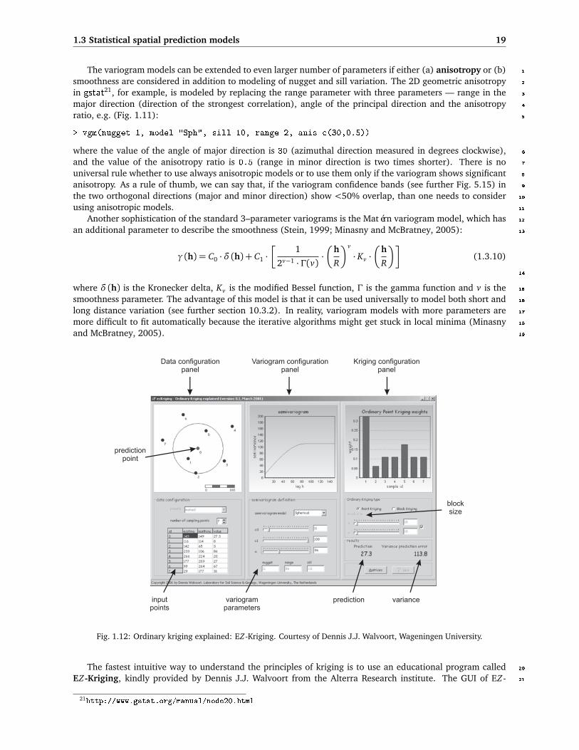
1.3 Statistical spatial prediction models 19
The variogram models can be extended to even larger number of parameters if either (a) anisotropy or (b) 1
smoothness are considered in addition to modeling of nugget and sill variation. The 2D geometric anisotropy 2
in gstat21, for example, is modeled by replacing the range parameter with three parameters — range in the 3
major direction (direction of the strongest correlation), angle of the principal direction and the anisotropy 4
ratio, e.g. (Fig. 1.11): 5
> vgm(nugget=1, model="Sph", sill=10, range=2, anis=c(30,0.5))
where the value of the angle of major direction is 30 (azimuthal direction measured in degrees clockwise), 6
and the value of the anisotropy ratio is 0.5 (range in minor direction is two times shorter). There is no 7
universal rule whether to use always anisotropic models or to use them only if the variogram shows significant 8
anisotropy. As a rule of thumb, we can say that, if the variogram confidence bands (see further Fig. 5.15) in 9
the two orthogonal directions (major and minor direction) show <50% overlap, than one needs to consider 10
using anisotropic models. 11
Another sophistication of the standard 3–parameter variograms is the Matérn variogram model, which has 12
an additional parameter to describe the smoothness (Stein, 1999; Minasny and McBratney, 2005): 13
γ (h) = C0 ·δ (h) + C1 ·�
1
2v−1 ·Γ(v)·�
h
R
�v
· Kv ·�
h
R
��
(1.3.10)
14
where δ (h) is the Kronecker delta, Kv is the modified Bessel function, Γ is the gamma function and v is the 15
smoothness parameter. The advantage of this model is that it can be used universally to model both short and 16
long distance variation (see further section 10.3.2). In reality, variogram models with more parameters are 17
more difficult to fit automatically because the iterative algorithms might get stuck in local minima (Minasny 18
and McBratney, 2005). 19
Fig. 1.12: Ordinary kriging explained: EZ-Kriging. Courtesy of Dennis J.J. Walvoort, Wageningen University.
The fastest intuitive way to understand the principles of kriging is to use an educational program called 20
EZ-Kriging, kindly provided by Dennis J.J. Walvoort from the Alterra Research institute. The GUI of EZ- 21
21http://www.gstat.org/manual/node20.html

20 Geostatistical mapping
Kriging consists of three panels: (1) data configuration panel, (2) variogram panel, and (3) kriging panel1
(Fig. 1.12). This allows you to zoom into ordinary kriging and explore its main characterizes and behavior:2
how do weights change for different variogram models, how do data values affect the weights, how does3
block size affect the kriging results etc. For example, if you study how model shape, nugget, sill and range4
affect the kriging results, you will notice that, assuming some standard variogram model (zero nugget, sill at5
global variance and practical range at 10% of the largest distance), the weights will decrease exponentially22.6
This is an important characteristic of kriging because it allows us to limit the search window to speed up the7
calculation and put more emphasize on fitting the semivariances at shorter distances. Note also that, although8
it commonly leads to smoothing of the values, kriging is an exact and non-convex interpolator. It is exact9
because the kriging estimates are equal to input values at sampling locations, and it is non-convex because its10
predictions can be outside the data range, e.g. we can produce negative concentrations.11
Another important aspect of using kriging is the issue of the support size. In geostatistics, one can control12
the support size of the outputs by averaging multiple (randomized) point predictions over regular blocks of13
land. This is known as block prediction (Heuvelink and Pebesma, 1999). A problem is that we can sample14
elevations at point locations, and then interpolate them for blocks of e.g. 10×10 m, but we could also take15
composite samples and interpolate them at point locations. This often confuses GIS users because as well as16
using point measurements to interpolate values at regular point locations (e.g. by point kriging), and then17
display them using a raster map (see Fig. 1.8), we can also make spatial predictions for blocks of land (block18
kriging) and display them using the same raster model (Bishop and McBratney, 2001). For simplicity, in the19
case of block-kriging, one should always try to use a cell size that corresponds to the support size.20
1.3.2 Environmental correlation21
If some exhaustively-sampled explanatory variables or covariates are available in the area of interest and22
if they are significantly correlated with our target variable (spatial cross-correlation), and assuming that the23
point-values are not spatially auto-correlated, predictions can be obtained by focusing only on the deterministic24
part of variation:25
Z(s) = f�
qk(s)
+ ε (1.3.11)
26
where qk are the auxiliary predictors. This approach to spatial prediction has a strong physical interpretation.27
Consider Rowe and Barnes (1994) observation that earth surface energy-moisture regimes at all scales/sizes28
are the dynamic driving variables of functional ecosystems at all scales/sizes. The concept of vegetation/soil-29
environment relationships has frequently been presented in terms of an equation with six key environmental30
factors as:31
V × S[x , y, t] = f
s[x , y, t] c[x , y, t] o[x , y, t]
r[x , y, t] p[x , y, t] a[x , y, t](1.3.12)
32
where V stands for vegetation, S for soil, c stands for climate, o for organisms (including humans), r is relief,33
p is parent material or geology, a is age of the system, x , y are the coordinates and t is time dimension. This34
means that the predictors which are available over entire areas of interest can be used to predict the value35
of an environmental variable at unvisited locations — first by modeling the relationship between the target36
and explanatory environmental predictors at sample locations, and then by applying it to unvisited locations37
using the known value of the explanatory variables at those locations. Common explanatory environmental38
predictors used to map environmental variables are land surface parameters, remotely sensed images, and39
geological, soil and land-use maps (McKenzie and Ryan, 1999). Because many auxiliary predictors (see further40
section 4) are now also available at low or no cost, this approach to spatial prediction is ever more important41
(Pebesma, 2006; Hengl et al., 2007a).42
Functional relations between environmental variables and factors are in general unknown and the cor-43
relation coefficients can differ for different study areas, different seasons and different scales. However, in44
22In practice, often >95% of weights will be explained by the nearest 30–50 points. Only if the variogram is close to the pure nuggetmodel, the more distant points will receive more importance, but then the technique will produce poor predictions anyhow.

1.3 Statistical spatial prediction models 21
many cases, relations with environmental predictors often reflect causal linkage: deeper and more developed 1
soils occur at places of higher potential accumulation and lower slope; different type of forests can be found 2
at different slope expositions and elevations; soils with more organic matter can be found where the climate 3
is cooler and wetter etc. This makes this technique especially suitable for natural resource inventory teams 4
because it allows them to validate their empirical knowledge about the variation of the target features in the 5
area of interest. 6
There are (at least) four groups of statistical models that have been used to make spatial predictions with 7
the help of environmental factors (Chambers and Hastie, 1992; McBratney et al., 2003; Bishop and Minasny, 8
2005): 9
Classification-based models — Classification models are primarily developed and used when we are dealing 10
with discrete target variables (e.g. land cover or soil types). There is also a difference whether Boolean 11
(crisp) or Fuzzy (continuous) classification rules are used to create outputs. Outputs from the model 12
fitting process are class boundaries (class centres and standard deviations) or classification rules. 13
Tree-based models — Tree-based models (classification or regression trees) are often easier to interpret when 14
a mix of continuous and discrete variables are used as predictors (Chambers and Hastie, 1992). They 15
are fitted by successively splitting a data set into increasingly homogeneous groupings. Output from 16
the model fitting process is a decision tree, which can then be applied to make predictions of either 17
individual property values or class types for an entire area of interest. 18
Regression models — Regression analysis employs a family of functions called Generalized Linear Models 19
(GLMs), which all assume a linear relationship between the inputs and outputs (Neter et al., 1996). 20
Output from the model fitting process is a set of regression coefficients. Regression models can be 21
also used to represent non-linear relationships with the use of General Additive Models (GAMs). The 22
relationship between the predictors and targets can be solved using one-step data-fitting or by using 23
iterative data fitting techniques (neural networks and similar). 24
Each of the models listed above can be equally applicable for mapping of environmental variables and each 25
can exhibit advantages and disadvantages. For example, some advantages of using tree-based regression are 26
that they: (1) can handle missing values; (2) can use continuous and categorical predictors; (3) are robust 27
to predictor specification; and (4) make very limited assumptions about the form of the regression model 28
(Henderson et al., 2004). Some disadvantages of regression trees, on the other hand, are that they require 29
large data sets and completely ignore spatial position of the input points. 30
Fig. 1.13: Comparison of spatial prediction techniques for mapping Zinc (sampling locations are shown in Fig. 1.9). Notethat inverse distance interpolation (.id) and kriging (.ok) are often quite similar; the moving trend surface (.tr; 2ndorder polynomial) can lead to artifacts (negative values) — locally where the density of points is poor. The regression-based(.lm) predictions were produced using distance from the river as explanatory variable (see further §5).
A common regression-based approach to spatial prediction is multiple linear regression (Draper and 31
Smith, 1998; Kutner et al., 2004). Here, the predictions are again obtained by weighted averaging (compare 32

22 Geostatistical mapping
with Eq.(1.3.2)), this time by averaging the predictors:1
zOLS(s0) = b0 + b1 · q1(s0) + . . .+ bp · qp(s0) =p∑
k=0
βk · qk(s0); q0(s0)≡ 1 (1.3.13)
2
or in matrix algebra:3
zOLS(s0) = βT·q (1.3.14)
4
where qk(s0) are the values of the explanatory variables at the target location, p is the number of predictors5
or explanatory variables23, and βk are the regression coefficients solved using the Ordinary Least Squares:6
β =�
qT · q�−1· qT · z (1.3.15)
7
where q is the matrix of predictors (n× p + 1) and z is the vector of sampled observations. The prediction8
error of a multiple linear regression model is (Neter et al., 1996, p.210):9
σ2OLS(s0) =MSE ·
h
1+ qT0 ·�
qT · q�−1· q0
i
(1.3.16)
10
where MSE is the mean square (residual) error around the regression line:11
MSE =
n∑
i=1
�
z(si)− z(si)�2
n− 2(1.3.17)
12
and q0 is the vector of predictors at new, unvisited location. In the univariate case, the variance of the13
prediction error can also be derived using:14
σ2(s0) =MSE ·
1+1
n+
�
q(s0)− q�2
n∑
i=1
�
q(si)− q�2
=MSE ·�
1+ v(s0)�
(1.3.18)
15
where v is the curvature of the confidence band around the regression line. This reflects the amount of16
extrapolation in the feature space (Ott and Longnecker, 2001, p.570). It can be seen from Eq. (1.3.18) that17
the prediction error, for a given sampling intensity (n/A), depends on three factors:18
(1.) Mean square residual error (MSE);19
(2.) Spreading of points in the feature space∑�
q(si)− q�2;20
(3.) ‘Distance’ of the new observation from the centre of the feature space�
q(s0)− q�
.21
So in general, if the model is linear, we can decrease the prediction variance if we increase the spreading of22
the points in feature space. Understanding this principles allows us to prepare sampling plans that will achieve23
higher mapping precision and minimize extrapolation in feature space (see further §2.8).24
23To avoid confusion with geographical coordinates, we use the symbol q, instead of the more common x , to denote a predictor.

1.3 Statistical spatial prediction models 23
The sum of squares of residuals (SSE) can be used to determine the adjusted coefficient of multiple 1
determination (R2a), which describes the goodness of fit: 2
R2a = 1−
�
n− 1
n− p
�
·SSE
SSTO
= 1−�
n− 1
n− p
�
·�
1− R2�
(1.3.19)
3
where SSTO is the total sum of squares (Neter et al., 1996), R2 indicates amount of variance explained by the 4
model, whereas R2a adjusts for the number of variables (p) used. For many environmental mapping projects, a 5
R2a ≥0.85 is already a very satisfactory solution and higher values will typically only mean over-fitting of the 6
data (Park and Vlek, 2002). 7
The principle of predicting environmental variables using factors of climate, relief, geology and similar, is 8
often referred to as environmental correlation. The environmental correlation approach to mapping is a true 9
alternative to ordinary kriging (compare differences in generated patterns in Fig. 1.13). This is because both 10
approaches deal with different aspects of spatial variation: regression deals with the deterministic and kriging 11
with the spatially-correlated stochastic part of variation. 12
The biggest criticism of the pure regression approach to spatial prediction is that the position of points in 13
geographical space is completely ignored, both during model fitting and prediction. Imagine if we are dealing 14
with two point data sets where one data set is heavily clustered, while the other is well-spread over the area 15
of interest — a sophistication of simple non-spatial regression is needed to account for the clustering of the 16
points so that the model derived using the clustered points takes this property into account. 17
One way to account for this problem is to take the distance between the points into account during the esti- 18
mation of the regression coefficients. This can be achieved by using the geographically weighted regression 19
(Fotheringham et al., 2002). So instead of using the OLS estimation (Eq.1.3.15) we use: 20
βWLS =�
qT ·W · q�−1· qT ·W · z (1.3.20)
21
where W is a matrix of weights, determined using some distance decay function e.g.: 22
wi(si , s j) = σ2E · exp
�
−3 ·d2(si , s j)
k2
�
(1.3.21)
23
where σ2E is the level of variation of the error terms, d(si , s j) is the Euclidian distance between a sampled 24
point pair and k is known as the bandwidth, which determines the degree of locality — small values of k 25
suggest that correlation only occurs between very close point pairs and large values suggest that such effects 26
exist even on a larger spatial scale. Compare further with Eq.(2.1.3). The problem remains to select a search 27
radius (Eq.1.3.21) using objective criteria. As we will see further (§2.2), geographically weighted regression 28
can be compared with regression-kriging with a moving window where variograms and regression models are 29
estimated locally. 30
The main benefit of geographically weighted regression (GWR) is that this method enables researchers 31
to study local differences in responses to input variables. It therefore more often focuses on coefficients’ 32
explanation than on interpolation of the endogenous variables. By setting up the search radius (bandwidth) 33
one can investigate the impact of spatial proximity between the samples on the regression parameters. By 34
fitting the regression models using a moving window algorithm, one can also produce maps of regression 35
coefficients and analyze how much the regression model is dependent on the location. However, the coefficient 36
maps generated by GWR are usually too smooth to be true. According to Wheeler and Tiefelsdorf (2005) and 37
Griffith (2008), the two main problems with GWR are: (1) strong multicollinearity effects among coefficients 38
make the results even totally wrong, and (2) lose degrees of freedom in the regression model. Hence, spatial 39
hierarchical model under bayesian framework (Gelfand et al., 2003) and spatial filtering model (Griffith, 2008) 40
may be better structures for such analyzes than GWR. 41

24 Geostatistical mapping
1.3.3 Predicting from polygon maps1
A special case of environmental correlation is prediction from polygon maps i.e. stratified areas (different land2
use/cover types, geological units etc). Assuming that the residuals show no spatial auto-correlation, a value3
at a new location can be predicted by:4
z(s0) =n∑
i=1
wi · z(s); wi =
1/nk for x i ∈ k
0 otherwise(1.3.22)
5
where k is the unit identifier. This means that the weights within some unit will be equal so that the predictions6
are made by simple averaging per unit (Webster and Oliver, 2001):7
z(s0) = µk =1
nk
nk∑
i=1
z(si) (1.3.23)
8
Consequently, the output map will show only abrupt changes in the values between the units. The predic-9
tion variance of this prediction model is simply the within-unit variance:10
σ2(s0) =σ2
k
nk(1.3.24)
11
From Eq.(1.3.24) it is obvious that the precision of the technique will be maximized if the within-unit12
variation is infinitely small. Likewise, if the within-unit variation is as high as the global variability, the13
predictions will be as bad as predicting by taking any value from the normal distribution.14
Another approach to make predictions from polygon maps is to use multiple regression. In this case, the15
predictors (mapping units) are used as indicators:16
z(s0) = b1 ·MU1(s0) + . . .+ bk ·MUk(s0); MUk ∈ [0|1] (1.3.25)
17
and it can be shown that the OLS fitted regression coefficients will equal the mean values within each strata18
(bk = µ(MUk)), so that the Eqs.(1.3.25) and (1.3.23) are in fact equivalent.19
If, on the other hand, the residuals do show spatial auto-correlation, the predictions can be obtained20
by stratified kriging. This is basically ordinary kriging done separately for each strata and can often be21
impractical because we need to estimate a variogram for each of the k strata (Boucneau et al., 1998). Note22
that the strata or sub-areas need to be known a priori and they should never be derived from the data used to23
generate spatial predictions.24
1.3.4 Hybrid models25
Hybrid spatial prediction models comprise of a combination of the techniques listed previously. For example,26
a hybrid geostatistical model employs both correlation with auxiliary predictors and spatial autocorrelation27
simultaneously. There are two main sub-groups of hybrid geostatistical models (McBratney et al., 2003): (a)28
co-kriging-based and (b) regression-kriging-based techniques, but the list could be extended.29
Note also that, in the case of environmental correlation by linear regression, we assume some basic (ad-30
ditive) model, although the relationship can be much more complex. To account for this, a linear regression31
model can be extended to a diversity of statistical models ranging from regression trees, to General Additive32
Models and similar. Consequently, the hybrid models are more generic than pure kriging-based or regression-33
based techniques and can be used to represent both discrete and continuous changes in the space, both deter-34
ministic and stochastic processes.35
One can also combine deterministic, statistical and expert-based estimation models. For example, one36
can use a deterministic model to estimate a value of the variable, then use actual measurements to fit a37
calibration model, analyze the residuals for spatial correlation and eventually combine the statistical fitting38

1.4 Validation of spatial prediction models 25
and deterministic modeling (Hengl et al., 2007a). Most often, expert-based models are supplemented with 1
the actual measurements, which are then used to refine the rules, e.g. using neural networks (Kanevski et al., 2
1997). 3
1.4 Validation of spatial prediction models 4
OK or OLS variance (Eqs.1.3.6; and 1.3.18) is the statistical estimate of the model uncertainty. Note that the 5
‘true’ prediction power can only be assessed by using an independent (control) data set. The prediction error 6
is therefore often referred to as the precision of prediction. The true quality of a map can be best assessed 7
by comparing estimated values (z(s j)) with actual observations at validation points (z∗(s j)). Commonly, two 8
measures are most relevant here — (1) the mean prediction error (ME): 9
ME =1
l·
l∑
j=1
�
z(s j)− z∗(s j)�
; E{ME}= 0 (1.4.1)
10
and (2) the root mean square prediction error (RMSE): 11
RMSE =
√
√
√
√
1
l·
l∑
j=1
�
z(s j)− z∗(s j)�2
; E{RMSE}= σ(h= 0) (1.4.2)
12
where l is the number of validation points. We can also standardize the errors based on the prediction variance 13
estimated by the spatial prediction model: 14
RMNSE =
√
√
√
√
1
l·
l∑
j=1
�
z(s j)− z∗(s j)
σ j
�2
; E{RMNSE}= 1 (1.4.3)
15
In order to compare accuracy of prediction between variables of different types, the RMSE can also be 16
normalized by the total variation: 17
RMSEr =RMSE
sz(1.4.4)
18
which will show how much of the global variation budget has been explained by the model. As a rule of thumb, 19
a value of RMSEr that is close to 40% means a fairly satisfactory accuracy of prediction (R-square=85%). 20
Otherwise, if RMSEr >71%, this means that the model accounted for less than 50% of variability at the 21
validation points. Note also that ME, RMSE and RMNSE estimated at validation points are also only a sample 22
from a population of values — if the validation points are poorly sampled, our estimate of the map quality 23
may be equally poor. 24
Because collecting additional (independent) samples is often impractical and expensive, validation of pre- 25
diction models is most commonly done by using cross-validation i.e. by subsetting the original point set in 26
two data set — calibration and validation — and then repeating the analysis. There are several types of 27
cross-validation methods (Bivand et al., 2008, pp.221–226): 28
the k–fold cross-validation — the original sample is split into k equal parts and then each is used for 29
cross-validation; 30
leave-one-out cross-validation (LOO) — each sampling point is used for cross-validation; 31
Jackknifing — similar to LOO, but aims at estimating the bias of statistical analysis and not of predictions; 32
Both k–fold and the leave-one-out cross validation are implemented in the krige.cv method of gstat 33
package. The LOO algorithm works as follows: it visits a data point, predicts the value at that location by 34
kriging without using the observed value, and proceeds with the next data point. This way each individual 35

26 Geostatistical mapping
point is assessed versus the whole data set. The results of cross-validation can be visualised to pinpoint the1
most problematic points, e.g. exceeding three standard deviations of the normalized prediction error, and2
to derive a summary estimate of the map accuracy. In the case of many outliers and blunders in the input3
data, the LOO cross-validation might produce strange outputs. Hence many authors recommend 10–fold4
cross-validation as the most robust approach. Note also that cross-validation is not necessarily independent —5
points used for cross-validation are subset of the original sampling design, hence if the original design is biased6
and/or non-representative, then also the cross-validation might not reveal the true accuracy of a technique.7
However, if the sampling design has been generated using e.g. random sampling, it can be shown that also8
randomly taken subsets will be unbiased estimators of the true accuracy.9
To assess the accuracy of predicting categorical variables we can use the kappa statistics, which is a com-10
mon measure of classification accuracy (Congalton and Green, 1999; Foody, 2004). Kappa statistics measures11
the difference between the actual agreement between the predictions and ground truth and the agreement that12
could be expected by chance (see further p.135). In most remote sensing-based mapping projects, a kappa13
larger than 85% is considered to be a satisfactory result (Foody, 2004). The kappa is only a measure of the14
overall mapping accuracy. Specific classes can be analyzed by examining the percentage of correctly classified15
pixels per each class:16
Pc =
m∑
j=1
�
C(s j) = C(s j)�
m(1.4.5)
17
where Pc is the percentage of correctly classified pixels, C(s j) is the estimated class at validation locations (s j)18
and m is total number of observations of class c at validation points.19
Further reading:20
Æ Cressie, N.A.C., 1993. Statistics for Spatial Data, revised edition. John Wiley & Sons, New York, 416 p.21
Æ Goovaerts, P., 1997. Geostatistics for Natural Resources Evaluation (Applied Geostatistics). Oxford22
University Press, New York, 496 p.23
Æ Isaaks, E.H. and Srivastava, R.M. 1989. An Introduction to Applied Geostatistics. Oxford University24
Press, New York, 542 p.25
Æ Webster, R. and Oliver, M.A., 2001. Geostatistics for Environmental Scientists. Statistics in Practice.26
John Wiley & Sons, Chichester, 265 p.27
Æ http://www.wiley.co.uk/eoenv/ — The Encyclopedia of Environmetrics.28
Æ http://geoenvia.org — A research association that promotes use of geostatistical methods for en-29
vironmental applications.30
Æ http://www.iamg.org — International Association of Mathematical Geosciences.31
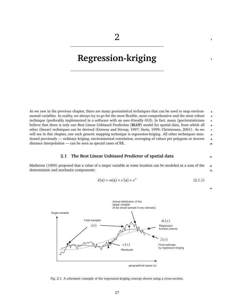
2 1
Regression-kriging 2
As we saw in the previous chapter, there are many geostatistical techniques that can be used to map environ- 3
mental variables. In reality, we always try to go for the most flexible, most comprehensive and the most robust 4
technique (preferably implemented in a software with an user-friendly GUI). In fact, many (geo)statisticians 5
believe that there is only one Best Linear Unbiased Prediction (BLUP) model for spatial data, from which all 6
other (linear) techniques can be derived (Gotway and Stroup, 1997; Stein, 1999; Christensen, 2001). As we 7
will see in this chapter, one such generic mapping technique is regression-kriging. All other techniques men- 8
tioned previously — ordinary kriging, environmental correlation, averaging of values per polygons or inverse 9
distance interpolation — can be seen as special cases of RK. 10
2.1 The Best Linear Unbiased Predictor of spatial data 11
Matheron (1969) proposed that a value of a target variable at some location can be modeled as a sum of the 12
deterministic and stochastic components: 13
Z(s) = m(s) + ε′(s) + ε′′ (2.1.1)
14
Fig. 2.1: A schematic example of the regression-kriging concept shown using a cross-section.
27

28 Regression-kriging
which he termed the universal model of spatial variation. We have seen in the previous sections (§1.3.1 and1
§1.3.2) that both deterministic and stochastic components of spatial variation can be modeled separately. By2
combining the two approaches, we obtain:3
z(s0) = m(s0) + e(s0)
=p∑
k=0
βk · qk(s0) +n∑
i=1
λi · e(si)(2.1.2)
4
where m(s0) is the fitted deterministic part, e(s0) is the interpolated residual, βk are estimated deterministic5
model coefficients (β0 is the estimated intercept), λi are kriging weights determined by the spatial dependence6
structure of the residual and where e(si) is the residual at location si . The regression coefficients βk can be7
estimated from the sample by some fitting method, e.g. ordinary least squares (OLS) or, optimally, using8
Generalized Least Squares (Cressie, 1993, p.166):9
βGLS =�
qT ·C−1 · q�−1· qT ·C−1 · z (2.1.3)
10
where βGLS is the vector of estimated regression coefficients, C is the covariance matrix of the residuals, q is11
a matrix of predictors at the sampling locations and z is the vector of measured values of the target variable.12
The GLS estimation of regression coefficients is, in fact, a special case of geographically weighted regression13
(compare with Eq.1.3.20). In this case, the weights are determined objectively to account for the spatial14
auto-correlation between the residuals.15
Once the deterministic part of variation has been estimated, the residual can be interpolated with kriging16
and added to the estimated trend (Fig. 2.1). Estimation of the residuals and their variogram model is an iter-17
ative process: first the deterministic part of variation is estimated using ordinary least squares (OLS), then the18
covariance function of the residuals is used to obtain the GLS coefficients. Next, these are used to re-compute19
the residuals, from which an updated covariance function is computed, and so on (Schabenberger and Got-20
way, 2004, p.286). Although this is recommended as the proper procedure by many geostatisticians, Kitanidis21
(1994) showed that use of the covariance function derived from the OLS residuals (i.e. a single iteration) is22
often satisfactory, because it is not different enough from the function derived after several iterations; i.e. it23
does not affect the final predictions much. Minasny and McBratney (2007) reported similar results: it is often24
more important to use more useful and higher quality data than to use more sophisticated statistical methods.25
In some situations1 however, the model needs to be fitted using the most sophisticated technique to avoid26
making biased predictions.27
In matrix notation, regression-kriging is commonly written as (Christensen, 2001, p.277):28
zRK(s0) = qT0 · βGLS +λ
T0 · (z− q · βGLS) (2.1.4)
29
where z(s0) is the predicted value at location s0, q0 is the vector of p+ 1 predictors and λ0 is the vector of n30
kriging weights used to interpolate the residuals. The model in Eq.(2.1.4) is considered to be the Best Linear31
Predictor of spatial data (Christensen, 2001; Schabenberger and Gotway, 2004). It has a prediction variance32
that reflects the position of new locations (extrapolation effect) in both geographical and feature space:33
σ2RK(s0) = (C0 + C1)− cT
0 ·C−1 · c0 +
�
q0 − qT ·C−1 · c0
�T·�
qT ·C−1 · q�−1·�
q0 − qT ·C−1 · c0
�
(2.1.5)
34
where C0 + C1 is the sill variation and c0 is the vector of covariances of residuals at the unvisited location.35
1For example: if the points are extremely clustered, and/or if the sample is�100, and/or if the measurements are noisy or obtainedusing non-standard techniques.

2.1 The Best Linear Unbiased Predictor of spatial data 29
Fig. 2.2: Whether we will use pure regression model, pure kriging or hybrid regression-kriging is basically determined byR-square: (a) if R-square is high, then the residuals will be infinitively small; (c) if R-square is insignificant, then we willprobably finish with using ordinary kriging; (b) in most cases, we will use a combination of regression and kriging.
If the residuals show no spatial auto-correlation (pure nugget effect), the regression-kriging (Eq.2.1.4) 1
converges to pure multiple linear regression (Eq.1.3.14) because the covariance matrix (C) becomes identity 2
matrix: 3
C=
C0 + C1 · · · 0... C0 + C1 0
0 0 C0 + C1
= (C0 + C1) · I (2.1.6)
4
so the kriging weights (Eq.1.3.4) at any location predict the mean residual i.e. 0 value. Similarly, the regression- 5
kriging variance (Eq.2.1.5) reduces to the multiple linear regression variance (Eq.1.3.16): 6
σ2RK(s0) = (C0 + C1)− 0+ qT
0 ·�
qT ·1
(C0 + C1)· q�−1
· q0
σ2RK(s0) = (C0 + C1) + (C0 + C1) · qT
0 ·�
qT · q�−1· q0
7
and since (C0 + C1) = C(0) =MSE, the RK variance reduces to the MLR variance: 8
σ2RK(s0) = σ
2OLS(s0) =MSE ·
h
1+ qT0 ·�
qT · q�−1· q0
i
(2.1.7)
9
Likewise, if the target variable shows no correlation with the auxiliary predictors, the regression-kriging 10
model reduces to ordinary kriging model because the deterministic part equals the (global) mean value 11
(Fig. 2.2c, Eq.1.3.25). 12
The formulas above show that, depending on the strength of the correlation, RK might turn into pure 13
kriging — if predictors are uncorrelated with the target variable — or pure regression — if there is significant 14
correlation and the residuals show pure nugget variogram (Fig. 2.2). Hence, pure kriging and pure regression 15
should be considered as only special cases of regression-kriging (Hengl et al., 2004a, 2007a). 16

30 Regression-kriging
2.1.1 Mathematical derivation of BLUP1
Understanding how a prediction model is derived becomes important once we start getting strange results or2
poor cross-validation scores. Each model is based on some assumptions that need to be respected and taken3
into account during the final interpretation of results. A detailed derivation of the BLUP for spatial data can be4
followed in several standard books on geostatistics (Stein, 1999; Christensen, 2001); one of the first complete5
derivations is given by Goldberger (1962). Here is a somewhat shorter explanation of how BLUP is derived,6
and what the implications of various mathematical assumptions are.7
All flavors of linear statistical predictors share the same objective of minimizing the estimation error vari-8
ance σ2E(s0) under the constraint of unbiasedness (Goovaerts, 1997). In mathematical terms, the estimation9
error:10
σ2(s0) = E¦
�
z(s0)− z(s0)�
·�
z(s0)− z(s0)�T© (2.1.8)
11
is minimized under the (unbiasedness) constraint that:12
E�
z(s0)− z(s0)
= 0 (2.1.9)
13
Assuming the universal model of spatial variation, we can define a generalized linear regression model14
(Goldberger, 1962):15
z(s) = qT · β + ε(s) (2.1.10)
E {ε(s)}= 0 (2.1.11)
E¦
ε · εT(s)©
= C (2.1.12)
16
where ε is the residual variation, and C is the n×n positive-definite variance-covariance matrix of residuals.17
This model can be read as follows: (1) the information signal is a function of deterministic and residual parts;18
(2) the best estimate of the residuals is 0; (3) the best estimate of the correlation structure of residuals is the19
variance-covariance matrix.20
Now that we have defined the statistical model and the minimization criteria, we can derive the best linear21
unbiased prediction of the target variable:22
z(s0) = δT0 · z (2.1.13)
23
Assuming that we use the model shown in Eq.(2.1.10), and assuming that the objective is to minimize24
the estimation error σ2E(s0), it can be shown2 that BLUP parameters can be obtained by solving the following25
system:26
C q
qT 0
·
δ
φ
=
c0
q0
(2.1.14)
27
where c0 is the vector of n×1 covariances at a new location, q0 is the vector of p×1 predictors at a new28
location, and φ is a vector of Lagrange multipliers. It can be further shown that, by solving the Eq.(2.1.14),29
we get the following:30
2The actual derivation of formulas is not presented. Readers are advised to obtain the paper by Goldberger (1962).

2.1 The Best Linear Unbiased Predictor of spatial data 31
z(s0) = qT0 · β + λ
T0 · (z− q · β)
β =�
qT ·C−1 · q�−1· qT ·C−1 · z (2.1.15)
λ0 = C−1 · c0
1
which is the prediction model explained in the previous section. 2
Under the assumption of the first order stationarity i.e. constant trend: 3
E {z(s)}= µ ∀s ∈ A (2.1.16)
4
the Eq.(2.1.15) modifies to (Schabenberger and Gotway, 2004, p.268): 5
z(s0) = µ+ λT0 · (z−µ)
λ0 = C−1 · c0
6
i.e. to ordinary kriging (§1.3.1). If we assume that the deterministic part of variation is not constant, then we 7
need to consider obtaining a number of covariates (q) that can be used to model the varying mean value. 8
Another important issue you need to know about the model in Eq.(2.1.15) is that, in order to solve the 9
residual part of variation, we need to know covariances at new locations: 10
C�
e(s0), e(si)�
= E��
e(s0)−µ
·�
e(si)−µ�
(2.1.17)
11
which would require that we know the values of the target variable at a new location (e(s0)), which we of 12
course do not know. Instead, we can use the existing sampled values (e(si) = z(si) − z(si)) to model the 13
covariance structure using a pre-defined mathematical model (e.g. Eq.1.3.8). If we assume that the covariance 14
model is the same (constant) in the whole area of interest, then the covariance is dependent only on the 15
separation vector h: 16
C�
e(s0), e(si)�
= C(h) (2.1.18)
17
which is known as the assumption of second order stationarity; and which means that we can use the 18
same model to predict values anywhere in the area of interest (global estimation). If this assumption is not 19
correct, we would need to estimate covariance models locally. This is often not so trivial because we need to 20
have a lot of points (see further §2.2), so the assumption of second order stationarity is very popular among 21
geostatisticians. Finally, you need to also be aware that the residuals in Eq.(2.1.10) are expected to be normally 22
distributed around the regression line and homoscedastic3, as with any linear regression model (Kutner et al., 23
2004). If this is not the case, then the target variable needs to be transformed until these conditions are met. 24
The first and second order stationarity, and normality of residuals/target variables are rarely tested in 25
real case studies. In the case of regression-kriging (see further §2.1), the target variable does not have to be 26
stationary but its residuals do, hence we do not have to test this property with the original variable. In the case 27
of regression-kriging in a moving window, we do not have to test neither first nor second order stationarity. 28
Furthermore, if the variable is non-normal, then we can use some sort of GLM to fit the model. If this is 29
successful, the residuals will typically be normal around the regression line in the transformed space, and this 30
will allow us to proceed with kriging. The predicted values can finally be back-transformed to the original 31
scale using the inverse of the link function. 32
3Meaning symmetrically distributed around the feature space and the regression line.

32 Regression-kriging
The lesson learned is that each statistical spatial predictor comes with: (a) a conceptual model that explains1
the general relationship (e.g. Eq.2.1.10); (b) model-associated assumptions (e.g. zero mean estimation error,2
first or second order stationarity, normality of the residuals); (c) actual prediction formulas (Eq.2.1.15); and3
(d) a set of proofs that, under given assumptions, a prediction model is the BLUP. Ignoring the important model4
assumptions can lead to poor predictions, even though the output maps might appear to be visually fine.5
2.1.2 Selecting the right spatial prediction technique6
Knowing that the most of the linear spatial prediction models are more or less connected, we can start by7
testing the most generic technique, and then finish by using the most suitable technique for our own case8
study. Pebesma (2004, p.689), for example, implemented such a nested structure in his design of the gstat9
package. An user can switch between one and another technique by following a simple decision tree shown in10
Fig. 2.3.11
YESIs the
variable correlatedwith environmental
factors?
NO
YESIs thephysical model
known?
NO
ORDINARYKRIGING
YESDo the
residuals showspatial auto-correlation?
YESDo the
residuals showspatial auto-correlation?
YESDoes the
variable showsspatial auto-correlation?
NO
MECHANICALINTERPOLATORS
YESCan a
variogram with >1parametersbe fitted?
NO
ENVIRONMENTALCORRELATION
(OLS)
REGRESSION-KRIGING
(calibration)
NO SPATIALPREDICTIONPOSSIBLE
REGRESSION-KRIGING
(GLS)
DETERMINISTICMODEL
NO
NO
Fig. 2.3: A general decision tree for selecting the suitable spatialprediction model based on the results of model estimation. Similardecision tree is implemented in the gstat package.
First, we need to check if the deterministic12
model is defined already, if it has not been, we13
can try to correlate the sampled variables with14
environmental factors. If the environmental15
factors are significantly correlated, we can fit16
a multiple linear regression model (Eq.1.3.14)17
and then analyze the residuals for spatial au-18
tocorrelation. If the residuals show no spa-19
tial autocorrelation (pure nugget effect), we20
proceed with OLS estimation of the regression21
coefficients. Otherwise, if the residuals show22
spatial auto-correlation, we can run regression-23
kriging. If the data shows no correlation with24
environmental factors, then we can still ana-25
lyze the variogram of the target variable. This26
time, we might also consider modeling the27
anisotropy. If we can fit a variogram different28
from pure nugget effect, then we can run or-29
dinary kriging. Otherwise, if we can only fit a30
linear variogram, then we might just use some31
mechanical interpolator such as the inverse dis-32
tance interpolation.33
If the variogram of the target variable34
shows no spatial auto-correlation, and no cor-35
relation with environmental factors, this practi-36
cally means that the only statistically valid pre-37
diction model is to estimate a global mean for38
the whole area. Although this might frustrate39
you because it would lead to a nonsense map where each pixel shows the same value, you should be aware40
that even this is informative4.41
How does the selection of the spatial prediction model works in practice? In the gstat package, a user can42
easily switch from one to other prediction model by changing the arguments in the generic krige function in43
R (Fig. 1.13; see further §3.2). For example, if the name of the input field samples is meuse and the prediction44
locations (grid) is defined by meuse.grid, we can run the inverse distance interpolation (§1.2.1) by specifying45
(Pebesma, 2004):46
> library(gstat)> data(meuse)> coordinates(meuse) <- ∼ x+y> data(meuse.grid)> coordinates(meuse.grid) <- ∼ x+y
4Sometimes an information that we are completely uncertain about a feature is better than a colorful but completely unreliable map.

2.1 The Best Linear Unbiased Predictor of spatial data 33
> gridded(meuse.grid) <- TRUE> zinc.id <- krige(zinc ∼ 1, data=meuse, newdata=meuse.grid)
[inverse distance weighted interpolation]
where zinc is the sampled environmental variable (vector) and zinc.id is the resulting raster map (shown 1
in Fig. 1.13). Instead of using inverse distance interpolation we might also try to fit the values using the 2
coordinates and a 2nd order polynomial model: 3
> zinc.ts <- krige(zinc ∼ x+y+x*y+x*x+y*y, data=meuse, newdata=meuse.grid)
[ordinary or weighted least squares prediction]
which can be converted to the moving surface fitting by adding a search window: 4
> zinc.mv <- krige(zinc ∼ x+y+x*y+x*x+y*y, data=meuse, newdata=meuse.grid, nmax=20)
[ordinary or weighted least squares prediction]
If we add a variogram model, then gstat will instead of running inverse distance interpolation run ordinary 5
kriging (§1.3.1): 6
> zinc.ok <- krige(log1p(zinc) ∼ 1, data=meuse, newdata=meuse.grid,+ model=vgm(psill=0.714, "Exp", range=449, nugget=0))
[using ordinary kriging]
where vgm(psill=0.714, "Exp", range=449, nugget=0) is the Exponential variogram model with a sill 7
parameter of 0.714, range parameter of 449 m and the nugget parameter of 0 (the target variable was log- 8
transformed). Likewise, if there were environmental factors significantly correlated with the target variable, 9
we could run OLS regression (§1.3.2) by omitting the variogram model: 10
> zinc.ec <- krige(log1p(zinc) ∼ dist+ahn, data=meuse, newdata=meuse.grid)
[ordinary or weighted least squares prediction]
where dist and ahn are the environmental factor used as predictors (raster maps), which are available as 11
separate layers within the spatial layer5 meuse.grid. If the residuals do show spatial auto-correlation, then 12
we can switch to universal kriging (Eq.2.1.4) by adding the variogram: 13
> zinc.rk <- krige(log1p(zinc) ∼ dist+ahn, data=meuse, newdata=meuse.grid,+ model=vgm(psill=0.151, "Exp", range=374, nugget=0.055))
[using universal kriging]
If the model between the environmental factors and our target variable is deterministic, then we can use 14
the point samples to calibrate our predictions. The R command would then look something like this: 15
> zinc.rkc <- krige(zinc ∼ zinc.df, data=meuse, newdata=meuse.grid,+ model=vgm(psill=3, "Exp", range=500, nugget=0))
[using universal kriging]
where zinc.df are the values of the target variable estimated using a deterministic function. 16
In gstat, a user can also easily switch from estimation to simulations (§2.4) by adding to the command 17
above an additional argument: nsim=1. This will generate Sequential Gaussian Simulations using the same 18
prediction model. Multiple simulations can be generated by increasing the number set for this argument. In 19
addition, a user can switch from block predictions by adding argument block=100; and from global estimation 20
of weights by adding a search radius or maximum number of pairs, e.g. radius=1000 or nmax=60. 21
By using the automap6 package one needs to specify even less arguments. For example, the command: 22
5In R a SpatialGridDataframe object.6http://cran.r-project.org/web/packages/automap/

34 Regression-kriging
> zinc.rk <- autoKrige(log1p(zinc) ∼ dist, data=meuse, newdata=meuse.grid)
[using universal kriging]
will do much of the standard geostatistical analysis without any intervention from the user: it will filter the1
duplicate points where needed, estimate the residuals, then fit the variogram for the residuals, and generate2
the predictions at new locations. The results can be plotted in a single page in a form of a report. Such generic3
commands can significantly speed up data processing, and make it easier for a non-geostatistician to generate4
maps (see further section 2.10.3).5
In the intamap package7, one needs to set even less parameters to generate predictions from a variety of6
methods:7
> meuse$value <- log(meuse$zinc)> output <- interpolate(data=meuse, newdata=meuse.grid)
R 2009-11-11 17:09:14 interpolating 155 observations, 3103 prediction locations[Time models loaded...][1] "estimated time for copula 133.479866956255"Checking object ... OK
which gives the (presumably) best interpolation method8 for the current problem (value column), given the8
time available set with maximumTime.9
A more systematic strategy to select the right spatial prediction technique is to use objective criteria of10
mapping success (i.e. a posteriori criteria). From the application point of view, it can be said that there are11
(only) five relevant criteria to evaluate various spatial predictors (see also §1.4):12
(1.) the overall mapping accuracy, e.g. standardized RMSE at control points — the amount of variation13
explained by the predictor expressed in %;14
(2.) the bias, e.g. mean error — the accuracy of estimating the central population parameters;15
(3.) the model robustness, also known as model sensitivity — in how many situations would the algorithm16
completely fail / how much artifacts does it produces?;17
(4.) the model reliability — how good is the model in estimating the prediction error (how accurate is the18
prediction variance considering the true mapping accuracy)?;19
(5.) the computational burden — the time needed to complete predictions;20
From this five, you could derive a single composite measure that would then allow you to select ‘the21
optimal’ predictor for any given data set, but this is not trivial! Hsing-Cheng and Chun-Shu (2007) suggest a22
framework to select the best predictor in an automated way, but this work would need to be much extended.23
In many cases we simply finish using some naïve predictor — that is predictor that we know has a statistically24
more optimal alternative9, but this alternative is simply not practical.25
The intamap decision tree, shown in Fig. 2.4, is an example of how the selection of the method can be26
automated to account for (1) anisotropy, (2) specified observation errors, and (3) extreme values. This is27
a specific application primarily developed to interpolate the radioactivity measurements from the European28
radiological data exchange platform, a network of around 4000 sensors. Because the radioactivity measure-29
ments can often carry local extreme values, robust techniques need to be used to account for such effects.30
For example, Copula kriging10 methods can generate more accurate maps if extreme values are also present31
in the observations. The problem of using methods such as Copula kriging, however, is that they can often32
take even few hours to generate maps even for smaller areas. To minimize the risk of running into endless33
computing, the authors of the intamap decision tree have decided to select the prediction algorithm based on34
7http://cran.r-project.org/web/packages/intamap/8intamap automatically chooses between: (1) kriging, (2) copula methods, (3) inverse distance interpolation, projected spatial gaus-
sian process methods in the psgp package, (4) transGaussian kriging or yamamoto interpolation.9For example, instead of using the REML approach to variogram modeling, we could simply fit a variogram using weighted least
squares (see §1.3.1), and ignore all consequences (Minasny and McBratney, 2007).10Copula kriging is a sophistication of ordinary kriging; an iterative technique that splits the original data set and then re-estimates the
model parameters with maximization of the corresponding likelihood function (Bárdossy and Li, 2008).

2.1 The Best Linear Unbiased Predictor of spatial data 35
the interpolation result e.g. as a GML document or coverage. To encode the interpolationerror UncertML, a markup language for specifying information that is represented prob-abilistically, has been developed within the project, which OGC has currently released asan OGC Discussion Paper [8].
Observation errors
specified?
Extreme value
distribution?
Projected sparse
Gaussian process
Data (observations)
[Interpolation domain]
Anisotropy:
significant? Correct for it
Yes
No
No
No
Maximum Likelihood Maximum likelihood
Yes
Yes
Spatial aggregation
Reformatting
Coordinate reference sytems:
Reproject?
Output
Variogram model fitting
Sample variograms,
Ordinary krigingInterpolation: Copula kriging
Modelling:
Figure 2: Decision tree for the interpolation method choices in the interpolation processthat takes place in R. References in text.The R back end and interpolation decision tree The procedure for the statistical analysisof the data are implemented in R, the major open source environment for analysing sta-tistical data. As figure 1 shows, this is not noticeable for the user of the INTAMAP webprocessing service, as R is run in the back end. Interfacing R from the web processingservice by using the TCP/IP protocol (i.e., as a web service, using the Rserve package[7])has the advantage that the R process, doing the numerical work, may be running on adedicated computing cluster not directly connected to the internet. Multiple interpolationrequests at the same time will be executed in parallel. A second advantage of having allstatistical routines in the R environment is that it can be re-used independently of the WPSinterface, e.g. interactively on a PC, from a SOAP interface, or on a mobile device. Thedecision tree for choosing an interpolation method automatically is shown in Figure 2.In the context of the INTAMAP project, dedicated interpolation methods have been im-plemented for (i) detecting and correcting for anisotropy, (ii) dealing with extreme valuedistributions, (iii) dealing with known measurement errors.
Methods for network harmonisation were also developed, but are not part of the au-tomated interpolation framework, as this should be done before interpolation takes place.The same is true for outlier removal and monitoring network optimisation. With the soft-ware developed for INTAMAP, it would be relatively simple to customize the INTAMAPweb service and perform these manipulations.
4 OPERATIONAL PERFORMANCE
At the stage of writing this paper, the INTAMAP interpolation service is fully functional,and open for testing. During the testing period, the the following issues need to be further
Fig. 2.4: Decision tree used in the intamap interpolation service for automated mapping. After Pebesma et al. (2009).
the computational time. Hence the system first estimates the approximate time needed to run the prediction 1
using the most sophisticated technique; if this is above the threshold time, the system will switch to a more 2
naïve method (Pebesma et al., 2009). As a rule of thumb, the authors of intamap suggest 30 seconds as the 3
threshold time to accept automated generation of a map via a web-service. 4
2.1.3 The Best Combined Spatial Predictor 5
Assuming that a series of prediction techniques are mutually independent11, predictions can be generated as a 6
weighted average from multiple predictions i.e. by generating the Best Combined Spatial Prediction (BCSP): 7
zBCSP(s0) =zSP1(s0) ·
1σSP1(s0)
+ zSP2(s0) ·1
σSP2(s0)+ . . .+ zSPj(s0) ·
1σSPj(s0)
p∑
j=1
1σSPj(s0)
(2.1.19)
8
where σSPj(s0) is the prediction error estimated by the model (prediction variance), and p is the number 9
of predictors. For example, we can generate a combined prediction using OK and e.g. GLM-regression and 10
then sum-up the two maps (Fig. 2.5). The predictions will in some parts of the study are look more as 11
OK, in others more as GLM, which actually depicts extrapolation areas of both methods. This map is very 12
similar to predictions produced using regression-kriging (see further Fig. 5.9); in fact, one could probably 13
mathematically prove that under ideal conditions (absolute stationarity of residuals; no spatial clustering; 14
perfect linear relationship), BCSP predictions would equal the regression-kriging predictions. In general, the 15
map in the middle of Fig. 2.5 looks more as the GLM-regression map because this map is about 2–3 times 16
more precise than the OK map. It is important to emphasize that, in order to combine various predictors, we 17
do need to have an estimate of the prediction uncertainty, otherwise we are not able to assign the weights (see 18
further §7.5). In principle, linear combination of statistical techniques using the Eq.(2.1.19) above should be 19
avoided if a theoretical basis exists that incorporates such combination. 20
11If they do not use the same model parameters; if they treat different parts of spatial variation etc.

36 Regression-kriging
Fig. 2.5: Best Combined Spatial Predictor as weighted average of ordinary kriging (zinc.ok) and GLM regression(zinc.glm).
In the example above (GLM+OK), we assume that the predictions/prediction errors are independent, and1
they are probably not. In addition, a statistical theory exists that supports a combination of regression and2
kriging (see previously §2.1.1), so there is no need to run predictions separately and derive an unrealistic3
measure of model error. The BCSP can be only interesting for situations where there are indeed several4
objective predictors possible, where no theory exists that reflects their combination, and/or where fitting of5
individual models is faster and less troublesome than fitting of a hybrid model. For example, ordinary kriging6
can be speed-up by limiting the search radius, predictions using GLMs is also relatively inexpensive. External7
trend kriging using a GLM in geoRglm package might well be the statistically most robust technique you could8
possibly use, but it can also be beyond the computational power of your PC.9
The combined prediction error of a BCSP can be estimated as the smallest prediction error achieved by any10
of the prediction models:11
σBCSP(s0) =min¦
σSP1(s0), . . . , σSPj(s0)©
(2.1.20)
12
which is really an ad hoc formula and should be used only to visualize and depict problematic areas (highest13
prediction error).14
2.1.4 Universal kriging, kriging with external drift15
The geostatistical literature uses many different terms for what are essentially the same or at least very sim-16
ilar techniques. This confuses the users and distracts them from using the right technique for their mapping17
projects. In this section, we will show that both universal kriging, kriging with external drift and regression-18
kriging are basically the same technique. Matheron (1969) originally termed the technique Le krigeage uni-19
versel, however, the technique was intended as a generalized case of kriging where the trend is modeled as20
a function of coordinates. Thus, many authors (Deutsch and Journel, 1998; Wackernagel, 2003; Papritz and21
Stein, 1999) reserve the term Universal Kriging (UK) for the case when only the coordinates are used as predic-22
tors. If the deterministic part of variation (drift) is defined externally as a linear function of some explanatory23
variables, rather than the coordinates, the term Kriging with External Drift (KED) is preferred (Wackernagel,24
2003; Chiles and Delfiner, 1999). In the case of UK or KED, the predictions are made as with kriging, with25
the difference that the covariance matrix of residuals is extended with the auxiliary predictors qk(si)’s (Web-26
ster and Oliver, 2001, p.183). However, the drift and residuals can also be estimated separately and then27
summed. This procedure was suggested by Ahmed and de Marsily (1987); Odeh et al. (1995) later named it28
Regression-kriging, while Goovaerts (1997, §5.4) uses the term Kriging with a trend model to refer to a family29
of predictors, and refers to RK as Simple kriging with varying local means. Although equivalent, KED and RK30
differ in the computational steps used.31

2.1 The Best Linear Unbiased Predictor of spatial data 37
Let us zoom into the two variants of regression-kriging. In the case of KED, predictions at new locations 1
are made by: 2
zKED(s0) =n∑
i=1
wKEDi (s0)·z(si) (2.1.21)
3
for 4
n∑
i=1
wKEDi (s0)·qk(si) = qk(s0); k = 1, ..., p (2.1.22)
5
or in matrix notation: 6
zKED(s0) = δT0 · z (2.1.23)
7
where z is the target variable, qk ’s are the predictor variables i.e. values at a new location (s0), δ0 is the vector 8
of KED weights (wKEDi ), p is the number of predictors and z is the vector of n observations at primary locations. 9
The KED weights are solved using the extended matrices: 10
λKED0 =¦
wKED1 (s0), ..., wKED
n (s0),ϕ0(s0), ...,ϕp(s0)©T
= CKED−1 · cKED0
(2.1.24)
11
where λKED0 is the vector of solved weights, ϕp are the Lagrange multipliers, CKED is the extended covariance 12
matrix of residuals and cKED0 is the extended vector of covariances at a new location. 13
In the case of KED, the extended covariance matrix of residuals looks like this (Webster and Oliver, 2001, 14
p.183): 15
CKED =
C(s1, s1) · · · C(s1, sn) 1 q1(s1) · · · qp(s1)...
......
......
C(sn, s1) · · · C(sn, sn) 1 q1(sn) · · · qp(sn)
1 · · · 1 0 0 · · · 0
q1(s1) · · · q1(sn) 0 0 · · · 0...
... 0...
...
qp(s1) · · · qp(sn) 0 0 · · · 0
(2.1.25)
16
and cKED0 like this: 17
cKED0 =¦
C(s0, s1), ..., C(s0, sn), q0(s0), q1(s0), ..., qp(s0)©T
; q0(s0) = 1 (2.1.26)
18
Hence, KED looks exactly as ordinary kriging (Eq.1.3.2), except the covariance matrix and vector are 19
extended with values of auxiliary predictors. 20
In the case of RK, the predictions are made separately for the drift and residuals and then added back 21
together (Eq.2.1.4): 22

38 Regression-kriging
zRK(s0) = qT0 · βGLS +λ
T0 · e
1
It can be demonstrated that both KED and RK algorithms give exactly the same results (Stein, 1999; Hengl2
et al., 2007a). Start from KED where the predictions are made as in ordinary kriging using zKED(s0) = λTKED· z.3
The KED kriging weights (λTKED
) are obtained by solving the system (Wackernagel, 2003, p.179):4
C q
qT 0
·
λKED
φ
=
c0
q0
5
where φ is a vector of Lagrange multipliers. Writing this out yields:6
C ·λKED + q ·φ = c0
qT ·λKED = q0(2.1.27)
7
from which follows:8
qT ·λKED = qT ·C−1 · c0 − qT ·C−1 · q ·φ (2.1.28)
9
and hence:10
φ =�
qT ·C−1 · q�−1· qT ·C−1 · c0 −
�
qT ·C−1 · q�−1· q0 (2.1.29)
11
where the identity qT · λKED = q0 has been used. Substituting φ back into Eq. (2.1.27) shows that the KED12
weights equal (Papritz and Stein, 1999, p.94):13
λKED = C−1 · c0 −C−1 · q ·h
�
qT ·C−1 · q�−1· qT ·C−1 · c0 −
�
qT ·C−1 · q�−1· q0
i
= C−1 ·h
c0 + q ·�
qT ·C−1q·�−1·�
q0 − qT ·C−1 · c0
�
i (2.1.30)
14
Let us now turn to RK. Recall from Eq.(2.1.3) that the GLS estimate for the vector of regression coefficients15
is given by:16
βGLS =�
qT ·C−1 · q�−1· qT ·C−1 · z (2.1.31)
17
and weights for residuals by:18
λT0 = cT
0 ·C−1 (2.1.32)
19
and substituting these in RK formula (Eq.2.1.4) gives:20
= qT0 · βGLS +λ
T0 · (z− q · βGLS)
=h
qT0 ·�
qT ·C−1 · q�−1· qT ·C−1 + cT
0 ·C−1 − cT
0 ·C−1 · q ·
�
qT ·C−1q�−1· qT ·C−1
i
· z
= C−1 ·h
cT0 + qT
0 ·�
qT ·C−1 · q�−1· qT − cT
0 ·C−1 · q ·
�
qT ·C−1q�−1· qTi
· z
= C−1 ·h
c0 + q ·�
qT ·C−1 · q�−1·�
q0 − qT ·C−1c0
�
i
· z
(2.1.33)

2.1 The Best Linear Unbiased Predictor of spatial data 39
The left part of the equation is equal to Eq.(2.1.30), which proves that KED will give the same predictions 1
as RK if same inputs are used. A detailed comparison of RK and KED using the 5–points example in MS Excel 2
is also available as supplementary material12. 3
Although the KED seems, at first glance, to be computationally more straightforward than RK, the vari- 4
ogram parameters for KED must also be estimated from regression residuals, thus requiring a separate regres- 5
sion modeling step. This regression should be GLS because of the likely spatial correlation between residuals. 6
Note that many analyst use instead the OLS residuals, which may not be too different from the GLS residuals 7
(Hengl et al., 2007a; Minasny and McBratney, 2007). However, they are not optimal if there is any spatial 8
correlation, and indeed they may be quite different for clustered sample points or if the number of samples is 9
relatively small (�200). 10
A limitation of KED is the instability of the extended matrix in the case that the covariate does not vary 11
smoothly in space (Goovaerts, 1997, p.195). RK has the advantage that it explicitly separates trend estimation 12
from spatial prediction of residuals, allowing the use of arbitrarily-complex forms of regression, rather than the 13
simple linear techniques that can be used with KED (Kanevski et al., 1997). In addition, it allows the separate 14
interpretation of the two interpolated components. For these reasons the use of the term regression-kriging 15
over universal kriging has been advocated by the author (Hengl et al., 2007a). The emphasis on regression is 16
important also because fitting of the deterministic part of variation is often more beneficial for the quality of 17
final maps than fitting of the stochastic part (residuals). 18
2.1.5 A simple example of regression-kriging 19
The next section illustrates how regression-kriging computations work and compares it to ordinary kriging 20
using the textbook example from Burrough and McDonnell (1998, p.139-141), in which five measurements 21
are used to predict a value of the target variable (z) at an unvisited location (s0) (Fig. 2.6a). We extend this 22
example by adding a hypothetical explanatory data source: a raster image of 10×10 pixels (Fig. 2.6b), which 23
has been constructed to show a strong negative correlation with the target variable at the sample points. 24
Fig. 2.6: Comparison of ordinary kriging and regression-kriging using a simple example with 5 points (Burrough andMcDonnell, 1998, p.139–141): (a) location of the points and unvisited site; (b) values of the covariate q; (c) variogramfor target and residuals, (d) OLS and GLS estimates of the regression model and results of prediction for a 10×10 gridusing ordinary kriging (e) and regression-kriging (f). Note how the RK maps reflects the pattern of the covariate.
The RK predictions are computed as follows: 25
12http://spatial-analyst.net/book/RK5points

40 Regression-kriging
(1.) Determine a linear model of the variable as predicted by the auxiliary map q. In this case the correlation1
is high and negative with OLS coefficients b0=6.64 and b1=-0.195 (Fig. 2.6d).2
(2.) Derive the OLS residuals at all sample locations as:3
e∗(si) = z(si)−�
b0 + b1 · q(si)�
(2.1.34)
For example, the point at (x=9, y=9) with z=2 has a prediction of 6.64− 0.195 · 23= 1.836, resulting4
in an OLS residual of e∗ =−0.164.5
(3.) Model the covariance structure of the OLS residuals. In this example the number of points is far6
too small to estimate the autocorrelation function, so we follow the original text in using a hypothetical7
variogram of the target variable (spherical model, nugget C0=2.5, sill C1=7.5 and range R=10) and8
residuals (spherical model, C0=2, C1=4.5, R=5). The residual model is derived from the target variable9
model of the text by assuming that the residual variogram has approximately the same form and nugget10
but a somewhat smaller sill and range (Fig. 2.6c), which is often found in practice (Hengl et al., 2004a).11
(4.) Estimate the GLS coefficients using Eq.(2.1.3). In this case we get just slightly different coefficients12
b0=6.68 and b1=-0.199. The GLS coefficients will not differ much from the OLS coefficients as long13
there is no significant clustering of the sampling locations (Fig. 2.6d) as in this case.14
(5.) Derive the GLS residuals at all sample locations:15
e∗∗(si) = z(si)−�
b0 + b1 · q(si)�
(2.1.35)
Note that the b now refer to the GLS coefficients.16
(6.) Model the covariance structure of the GLS residuals as a variogram. In practice this will hardly differ17
from the covariance structure of the OLS residuals.18
(7.) Interpolate the GLS residuals using ordinary kriging (OK) using the modeled variogram13. In this19
case at the unvisited point location (5, 5) the interpolated residual is −0.081.20
(8.) Add the GLS surface to the interpolated GLS residuals at each prediction point. At the unvisited point21
location (5,5) the explanatory variable has a value 12, so that the prediction is then:22
z(5, 5) = b0 + b1 · qi +n∑
i=1
λi(s0)·e(si)
= 6.68− 0.199 · 12− 0.081= 4.21
(2.1.36)
which is, in this specific case, a slightly different result than that derived by OK with the hypothetical23
variogram of the target variable (z=4.30).24
The results of OK (Fig. 2.6e) and RK (Fig. 2.6f) over the entire spatial field are quite different in this case,25
because of the strong relation between the covariate and the samples. In the case of RK, most of variation in26
the target variable (82%) has been accounted for by the predictor. Unfortunately, this version of RK has not27
been implemented in any software package yet14 (see further §3.4.3). Another interesting issue is that most28
of the software in use (gstat, SAGA) does not estimate variogram using the GLS estimation of the residuals,29
but only of the OLS residuals (0 iterations). Again, for most of balanced and well spread sample sets, this will30
not cause any significant problems (Minasny and McBratney, 2007).31
13Some authors argue whether one should interpolate residuals using simple kriging with zero expected mean of the residuals (bydefinition) or by ordinary kriging. In the case of OLS estimation, there is no difference; otherwise one should always use OK to avoidmaking biased estimates.
14Almost all geostatistical packages implement the KED algorithm because it is mathematically more elegant and hence easier toprogram.

2.2 Local versus localized models 41
2.2 Local versus localized models 1
Fig. 2.7: Local regression-kriging is a further sophistication ofregression-kriging. It will largely depend on the availabilityof explanatory and field data.
In many geostatistical packages, a user can opt to 2
limit the selection of points to determine the kriging 3
weights by setting up a maximum distance and/or 4
minimum and maximum number of point pairs (e.g. 5
take only the closest 50 points). This way, the cal- 6
culation of the new map can be significantly speed 7
up. In fact, kriging in global neighborhood where 8
n �1000 becomes cumbersome because of compu- 9
tation of C−1 (Eq.1.3.5). Recall from §1.3.1 that the 10
importance of points (in the case of ordinary kriging 11
and assuming a standard initial variogram model) 12
exponentially decreases with their distance from the 13
point of interest. Typically, geostatisticians suggest 14
that already first 30–60 closest points will be good 15
enough to obtain stable predictions. 16
A prediction model where the search radius for 17
derivation of kriging weights (Eq.1.3.4) is limited to 18
a local neighborhood can be termed localized pre- 19
diction model. There is a significant difference be- 20
tween localized and local prediction model, which of- 21
ten confuses inexperienced users. For example, if we set a search radius to re-estimate the variogram model, 22
then we speak about a local prediction model, also known as the moving window kriging or kriging using 23
local variograms (Haas, 1990; Walter et al., 2001; Lloyd, 2009). The local prediction model assumes that the 24
variograms (and regression models) are non-stationary, i.e. that they need to be estimated locally. 25
Fig. 2.8: Local variogram modeling and local ordinary kriging using a moving window algorithm in Vesper: a user canvisually observe how the variograms change locally. Courtesy of Budiman Minasny.
While localized prediction models are usually just a computational trick to speed up the calculations, 26
local prediction models are computationally much more demanding. Typically, they need to allow automated 27

42 Regression-kriging
variogram modeling and filtering of improbable models to prevent artifacts in the final outputs. A result of1
local prediction model (e.g. moving window variogram modeling) are not only maps of predictions, but also2
spatial distribution of the fitted variogram parameters (Fig. 2.7). This way we can observe how does the3
nugget variation changes locally, which parts of the area are smooth and which are noisy etc. Typically, local4
variogram modeling and prediction make sense only when we work with large point data sets (e.g.�1000 of5
field observations), which is still not easy to find. In addition, local variogram modeling is not implemented in6
many packages. In fact, the author is aware of only one: Vesper15 (Fig. 2.8).7
In the case of regression-kriging, we could also run both localized and local models. This way we will not8
only produce maps of variogram parameters but we would also be able to map the regression coefficients16.9
In the case of kriging with external drift, some users assume that the same variogram model can be used in10
various parts of the study area and limit the search window to speed up the calculations17. This is obviously11
a simplification, because in the case of KED both regression and kriging part of predictions are solved at the12
same time. Hence, if we limit the search window, but keep a constant variogram model, we could obtain13
very different predictions then if we use the global (regression-kriging) model. Only if the variogram of14
residuals if absolutely stationary, then we can limit the search window to fit the KED weights. In practice, either15
global (constant variogram) or local prediction models (locally estimated regression models and variograms16
of residuals) should be used for KED model fitting.17
2.3 Spatial prediction of categorical variables18
Fig. 2.9: Difficulties of predicting point-class data (b) and (d), as com-pared to quantitative variables (a) and (c), is that the class-interpolatorsare typically more complex and computationally more time-consuming.
Although geostatistics is primarily in-19
tended for use with continuous environ-20
mental variables, it can also be used to21
predict various types of categorical or22
class-type variables. Geostatistical anal-23
ysis of categorical variables is by many24
referred to as the indicator geostatis-25
tics (Bierkens and Burrough, 1993). In26
practice, indicator kriging leads to many27
computational problems, which probably28
explains why there are not many opera-29
tional applications of geostatistical map-30
ping of categorical variables in the world31
(Hession et al., 2006). For example, it32
will typically be difficult to fit variogram33
for less frequent classes that occur at iso-34
lated locations (Fig. 2.9d).35
Statistical grounds of indicator geo-36
statistics has been recently reviewed by37
Papritz et al. (2005); Papritz (2009) who38
recognizes several conceptual difficulties39
of working with indicator data: (1) incon-40
sistent modeling of indicator variograms,41
and (2) use of global variogram leads to biased predictions because the residuals are by definition non-42
stationary. Any attempt to use indicator kriging for data with an apparent trend either explicitly or implic-43
itly by using ordinary indicator kriging within a local neighborhood requires the modeling of non-stationary44
indicator variograms to preserve the mean square optimality of kriging (Papritz, 2009). Indicator regression-45
kriging without any transformation has also been criticized because the model (binomial variable) suggests46
that residuals have mean-dependent variance (p · (1− p)), and thus using a single variogram for the full set of47
residuals is not in accordance with theory.48
Let us denote the field observations of a class-type variable as zc(s1), zc(s2), ..., zc(sn), where c1, c2,..., ck are49
discrete categories (or states) and k is the total number of classes. A technique that estimates the soil-classes50
15http://www.usyd.edu.au/su/agric/acpa/vesper/vesper.html16Regression coefficients are often mapped with geographically weighted regression (Griffith, 2008).17Software such as gstat and SAGA allow users to limit the search radius; geoR does not allow this flexibility.

2.3 Spatial prediction of categorical variables 43
at new unvisited location zc(s0), given the input point data set (zc(s1), zc(s2), ..., zc(sn)), can then be named a 1
class-type interpolator. If spatially exhaustive predictors q1, q2, ..., qp (where p is the number of predictors) are 2
available, they can be used to map each category over the area of interest. So far, there is a limited number of 3
techniques that can achieve this: 4
Multi-indicator co-kriging — The simple multi-indicator kriging can also be extended to a case where several 5
covariates are used to improve the predictions. This technique is known by the name indicator (soft) 6
co-kriging (Journel, 1986). Although the mathematical theory is well explained (Bierkens and Burrough, 7
1993; Goovaerts, 1997; Pardo-Iguzquiza and Dowd, 2005), the application is cumbersome because of 8
the need to fit a very large number of cross-covariance functions. 9
Multinomial Log-linear regression — This a generalization of logistic regression for situations when there 10
are multiple classes of a target variable (Venables and Ripley, 2002). Each class gets a separate set of 11
regression coefficients (βc). Because the observed values equal either 0 or 1, the regression coefficients 12
need to be solved through a maximum likelihood iterative algorithm (Bailey et al., 2003), which makes 13
the whole method somewhat more computationally demanding than simple multiple regression. An 14
example of multinomial regression is given further in section 9.6. 15
Regression-kriging of indicators — One approach to interpolate soil categorical variables is to first assign 16
memberships to point observations and then to interpolate each membership separately. This approach 17
was first elaborated by de Gruijter et al. (1997) and then applied by Bragato (2004) and Triantafilis et al. 18
(2001). An alternative is to first map cheap, yet descriptive, diagnostic distances and then classify these 19
per pixel in a GIS (Carré and Girard, 2002). 20
In the case of logistic regression, the odds to observe a class (c) at new locations are computed as: 21
z+c (s0) =�
1+ exp�
−βcT · q0
��−1; c = 1,2, .., k (2.3.1)
22
where z+c (s0) are the estimated odds for class (c) at a new location s0 and k is the number of classes. The 23
multinomial logistic regression can also be extended to regression-kriging (for a complete derivation see Hengl 24
et al. (2007b)). This means that the regression modeling is supplemented with the modeling of variograms 25
for regression residuals, which can then be interpolated and added back to the regression estimate. So the 26
predictions are obtained using: 27
z+c (s0) =�
1+ exp�
−βcT · q0
��−1+ e+c (s0) (2.3.2)
28
where e+c are the interpolated residuals. The extension from multinomial regression to regression-kriging is not 29
as simple as it seems. This is because the estimated values at new locations in Eq.(2.3.2) are constrained within 30
the indicator range, which means that interpolation of residuals might lead to values outside the physical range 31
(<0 or >1)18. One solution to this problem is to predict the trend part in transformed space, then interpolate 32
residuals, sum the trend and residual part and back-transform the values (see §5.4). 33
Hengl et al. (2007b) show that memberships (µc), instead of indicators, are more suitable both for regres- 34
sion and geostatistical modeling, which has been also confirmed by several other authors (McBratney et al., 35
1992; de Gruijter et al., 1997; Triantafilis et al., 2001). Memberships can be directly linearized using the logit 36
transformation: 37
µ+c = ln�
µc
1−µc
�
; 0< µc < 1 (2.3.3)
38
where µc are the membership values used as input to interpolation. Then, all fitted values will be within the 39
physical range (0–1). The predictions of memberships for class c at new locations are then obtained using the 40
standard regression-kriging model (Eq.2.1.4): 41
µ+c (s0) = qT0 · βc,GLS +λ
Tc,0 ·�
µ+c − q · βc,GLS
�
(2.3.4)
18The degree to which they will fall outside the 0–1 range is controlled by the variogram and amount of extrapolation in feature space

44 Regression-kriging
The interpolated values can then be back-transformed to the membership range using (Neter et al., 1996):1
µc(s0) =eµ+c (s0)
1+ eµ+c (s0)(2.3.5)
2
In the case of regression-kriging of memberships, both spatial dependence and correlation with the pre-3
dictors are modeled in a statistically sophisticated way. In addition, regression-kriging of memberships allows4
fitting of each class separately, which facilitates the understanding of the distribution of soil variables and the5
identification of problematic classes, i.e. classes which are not correlated with the predictors or do not show6
any spatial autocorrelation etc.7
Spatial prediction of memberships can be excessive in computation time. Another problem is that, if the8
interpolated classes (odds, memberships) are fitted only by using the sampled data, the predictions of the9
odds/memberships will commonly not sum to unity at new locations. In this case, one needs to standardize10
values for each grid node by diving the original values by the sum of odds/memberships to ensure that they11
sum to unity, which is an ad-hoc solution. An algorithm, such as compositional regression-kriging19 will need12
to be developed.13
A number of alternative hybrid class-interpolators exists, e.g. the Bayesian Maximum Entropy (BME) ap-14
proach by D’Or and Bogaert (2005). Another option is to use Markov-chain algorithms (Li et al., 2004, 2005a).15
However, note that although use of the BME and Markov-chain type of algorithms is a promising development,16
their computational complexity makes it still far from use in operational mapping.17
2.4 Geostatistical simulations18
Regression-kriging can also be used to generate simulations of a target variable using the same inputs as in the19
case of spatial prediction system. An equiprobable realization of an environmental variable can be generated20
by using the sampled values and their variogram model:21
Z (SIM)(s0) = E¦
Z |z(s j),γ(h)©
(2.4.1)
22
where Z (SIM) is the simulated value at the new location. The most common technique in geostatistics that23
can be used to generate equiprobable realizations is the Sequential Gaussian Simulation (Goovaerts, 1997,24
p.380-392). It starts by defining a random path for visiting each node of the grid once. At first node, kriging is25
used to determine the location-specific mean and variance of the conditional cumulative distribution function.26
A simulated value can then be drawn by using the inverse normal distribution (Box and Muller, 1958; Banks,27
1998):28
zSIMi = zi + σi ·p
−2 · ln(1− A) · cos(2 ·π · B) (2.4.2)
29
where zSIMi is the simulated value of the target variable with induced error, A and B are the independent random30
numbers within the 0−0.99. . . range, zi is the estimated value at ith location, and σi is the regression-kriging31
error. The simulated value is then added to the original data set and the procedure is repeated until all nodes32
have been visited. Geostatistical simulations are used in many different fields to generate multiple realizations33
of the same feature (Heuvelink, 1998; Kyriakidis et al., 1999), or to generate realistic visualizations of a natural34
phenomena (Hengl and Toomanian, 2006; Pebesma et al., 2007). Examples of how to generate geostatistical35
simulations and use them to estimate the propagated error are further shown in section 10.3.2.36
2.5 Spatio-temporal regression-kriging37
In statistics, temporal processes (time series analysis, longitudinal data analysis) are well-known, but mixed38
spatio-temporal processes are still rather experimental (Banerjee et al., 2004). The 2D space models can be39
19Walvoort and de Gruijter (2001), for example, already developed a compositional solution for ordinary kriging that will enforceestimated values to sum to unity at all locations.

2.5 Spatio-temporal regression-kriging 45
extended to the time domain, which leads to spatio-temporal geostatistics (Kyriakidis and Journel, 1999). 1
The universal kriging model (Eq.2.1.1) then modifies to: 2
Z(s, t) = m(s, t) + ε′(s, t) + ε′′ (2.5.1)
3
where ε′(s, t) is the spatio-temporally autocorrelated residual for every (s, t) ∈ S × T , while m(s, t), the 4
deterministic component of the model, can be estimated using e.g. (Fassó and Cameletti, 2009): 5
m(s, t) = q(s, t) · β +K(s) · yt +ω(s, t) (2.5.2)
6
where q is a matrix of covariates available at all s, t locations, yt is a component of a target variable that is 7
constant in space (global trend), K(s) is a matrix of coefficients, andω(s, t) is the spatial small-scale component 8
(white noise in time) correlated over space. 9
A possible but tricky simplification of the space-time models is to consider time to be third dimension of 10
space. In that case, spatio-temporal interpolation follows the same interpolation principle as explained in 11
Eq.(1.1.2), except that here the variograms are estimated in three dimensions (two-dimensional position x 12
and y and ‘position’ in time). From the mathematical aspect, the extension from the static 2D interpolation 13
to the 3D interpolation is then rather simple. Regression modeling can be simply extended to a space-time 14
model by adding time as a predictor. For example, a spatio-temporal regression model for interpolation of land 15
surface temperature (see further §2.9.2) would look like this: 16
LST(s0, t0) = b0 + b1 ·DEM(s0) + b2 · LAT(s0) + b3 ·DISTC(s0) + b4 · LSR(s0, t0)
+ b5 · SOLAR(s0, t0) + b6 · cos�
[t0 −φ] ·π
180
�
; ∆t = 1 day(2.5.3)
17
Fig. 2.10: Extension of a 2D prediction model to the space-timedomain. Note that in the space-time cube, the amount of pixelsneeded to store the data exponentially increases as a function of:width × height × number of predictors × number of time intervals.
where DEM is the elevation map, LAT is the 18
map showing distance from the equator, DISTC 19
is the distance from the coast line, LSR is the 20
land surface radiation from natural or man- 21
made objects, SOLAR is the direct solar inso- 22
lation for a given cumulative Julian day t ∈ 23
(0,+∞), cos(t) is a generic function to ac- 24
count for seasonal variation of values and φ 25
is the phase angle20. DEM, LAT, DISTC are 26
temporally-constant predictors, while surface 27
radiation and solar insolation maps need to be 28
provided for each time interval used for data 29
fitting. 30
The residuals from this regression model 31
can then be analyzed for (spatio-temporal) 32
auto-correlation. In gstat, extension from 2D 33
to 3D variograms is possible by extending the 34
variogram parameters: for 3D space-time vari- 35
ograms five values should be given in the form 36
anis = c(p,q,r,s,t), where p is the angle 37
for the principal direction of continuity (mea- 38
sured in degrees, clockwise from y , in direction 39
of x), q is the dip angle for the principal di- 40
rection of continuity (measured in positive de- 41
grees up from horizontal), r is the third rota- 42
tion angle to rotate the two minor directions 43
20A time delay from the coldest day.

46 Regression-kriging
around the principal direction defined by p and q21 (see Fig. 1.11). A positive angle acts counter-clockwise1
while looking in the principal direction.2
Once we have fitted the space-time variogram, we can run regression-kriging to estimate the values at 3D3
locations. In practice, we only wish to produce maps for a given time interval (t0=constant), i.e. to produce4
2D-slices of values in time (Fig. 2.10). Once we have produced a time-series of predictions, we can analyze5
the successive time periods and run various types of time-series analysis. This will help us detect temporal6
trends spatially and extract informative images about the dynamics of the feature of interest.7
Note that, in order to yield accurate predictions using spatio-temporal techniques, dense sampling in both8
space and time is required. This means that existing natural resource surveys that have little to no repetition in9
time (�10 repetitions in time) cannot be adopted. Not to mention the computational complexity as the maps10
of predictors now multiply by the amount of time intervals. In addition, estimation of the spatio-temporal11
variograms will often be a cumbersome because we need to fit space-time models, for which we might not12
have enough space-time observations. A review of spatio-temporal models, i.e. dynamic linear state-space13
models, and some practical suggestions how to analyze such data and fit spatially varying coefficients can be14
followed in Banerjee et al. (2004, §8).15
A specific extension of the general model from Eq.(2.5.1) is to estimate the deterministic part of variation16
by using process-based (simulation) models, which are often based on differential equations. In this case an17
environmental variable is predicted from a set of environmental predictors incorporated in a dynamic model18
(Eq.1.3.12):19
Z(s, t) = fs,c,r,p,a(t) + ε′(s, t) + ε′′ (2.5.4)
20
where s, c, r, p, a are the input (zero-stage) environmental conditions and f is a mathematical deterministic21
function that can be used to predict the values for a given space-time position. This can be connected with the22
Einstein’s assumption that the Universe is in fact a trivial system that can be modeled and analyzed using “a23
one–dimensional differential equation — in which everything is a function of time”22. Some examples of op-24
erational soil-landscape process-based models are given by Minasny and McBratney (2001) and Schoorl et al.25
(2002). In vegetation science, for example, global modeling has proven to be very efficient for explanation of26
the actual distribution of vegetation and of global changes (Bonan et al., 2003). Integration of environmental27
process-based models will soon lead to development of a global dynamic model of environmental systems that28
would then provide solutions for different multipurpose national or continental systems.29
Fassó and Cameletti (2009) recently proposed hierarchical models as a general approach for spatio-temporal30
problems, including dynamical mapping, and the analysis of the outputs from complex environmental model-31
ing chains. The hierarchical models are a suitable solution to spatio-temporal modeling because they make it32
possible to define the joint dynamics and the full likelihood; the maximum likelihood estimation can be further33
simplified by using Expectation-Maximization algorithm. The basis of this approach is the classical two-stage34
hierarchical state-space model (Fassó and Cameletti, 2009):35
Zt = qt · β +K · yt + et (2.5.5)
yt = G · yt−1 +ηt (2.5.6)
36
where yt is modeled as the autoregressive process, G is the transition matrix and ηt is the innovation error. If37
all parameters are known, the unobserved temporal process yt can be estimated for each time point t using38
e.g. Kalman filter or Kalman smoother. Such process-based spatio-temporal models are still experimental and39
it make take time until their semi-automated software implementations appear in R.40
2.6 Species Distribution Modeling using regression-kriging41
The key inputs to a Species Distribution Model (SDM) are: the inventory (population) of animals or plants42
consisting of a total of N individuals (a point pattern X =�
siN
1 ; where si is a spatial location of individual43
21http://www.gstat.org/manual/node20.html22Quote by James Peebles, Princeton, 1990; published in “God’s Equation: Einstein, Relativity, and the Expanding Universe” by Amir D.
Aczel.

2.6 Species Distribution Modeling using regression-kriging 47
animal or plant; Fig. 1.3a), covering some area BHR ⊂ R2 (where HR stands for home-range and R2 is the 1
Euclidean space), and a list of environmental covariates/predictors (q1, q2, . . . qp) that can be used to explain 2
spatial distribution of a target species. In principle, there are two distinct groups of statistical techniques that 3
can be used to map the realized species’ distribution: (a) the point pattern analysis techniques, such as kernel 4
smoothing, which aim at predicting density of a point process (Fig. 2.11a); and (b) statistical, GLM-based, 5
techniques that aim at predicting the probability distribution of occurrences (Fig. 2.11c). Both approaches are 6
explained in detail in the following sections. 7
Fig. 2.11: Examples of (simulated) species distribution maps produced using common statistical models.
Species’ density estimation using kernel smoothing and covariates 8
Spatial density (ν; if unscaled, also known as “spatial intensity”) of a point pattern (ignoring the time dimen- 9
sion) is estimated as: 10
E [N(X∩ B)] =
∫
B
ν(s)ds (2.6.1)
11

48 Regression-kriging
In practice, it can be estimated using e.g. a kernel estimator (Diggle, 2003; Baddeley, 2008):1
ν(s) =n∑
i=1
κ ·�
s− si
�
· b(s) (2.6.2)
2
where ν(s) is spatial density at location s, κ(s) is the kernel (an arbitrary probability density), si is location of3
an occurrence record,
s− si
is the distance (norm) between an arbitrary location and observation location,4
and b(s) is a border correction to account for missing observations that occur when s is close to the border5
of the region (Fig. 2.11a). A common (isotropic) kernel estimator is based on a Gaussian function with mean6
zero and variance 1:7
bν(s) =1
H2 ·n∑
i=1
1p
2π· e−
‖s−si‖2
2 · b(s) (2.6.3)
8
The key parameter for kernel smoothing is the bandwidth (H) i.e. the smoothing parameter, which can be9
connected with the choice of variogram in geostatistics. The output of kernel smoothing is typically a map10
(raster image) consisting of M grid nodes, and showing spatial pattern of species’ clustering.11
Spatial density of a point pattern can also be modeled using a list of spatial covariates q’s (in ecology, we12
call this environmental predictors), which need to be available over the whole area of interest B. For example,13
using a Poisson model (Baddeley, 2008):14
logν(s) = logβ0 + log q1(s) + . . .+ log qp(s) (2.6.4)
15
where log transformation is used to account for the skewed distribution of both density values and covariates;16
p is the number of covariates. Models with covariates can be fitted to point patterns e.g. in the spatstat17
package23. Such point pattern–covariates analysis is commonly run only to determine i.e. test if the covariates18
are correlated with the feature of interest, to visualize the predicted trend function, and to inspect the spatial19
trends in residuals. Although statistically robust, point pattern–covariates models are typically not considered20
as a technique to improve prediction of species’ distribution. Likewise, the model residuals are typically not21
used for interpolation purposes.22
Predicting species’ distribution using ENFA and GLM (pseudo-absences)23
An alternative approach to spatial prediction of species’ distribution using occurrence-only records and envi-24
ronmental covariates is the combination of ENFA and regression modeling. In general terms, predictions are25
based on fitting a GLM:26
E(P) = µ= g−1(q · β) (2.6.5)
27
where E(P) is the expected probability of species occurrence (P ∈ [0,1]; Fig. 2.11c), q·β is the linear regression28
model, and g is the link function. A common link function used for SDM with presence observations is the29
logit link function:30
g(µ) = µ+ = ln�
µ
1−µ
�
(2.6.6)
31
and the Eq.(2.6.5) becomes logistic regression (Kutner et al., 2004).32
The problem of running regression analysis with occurrence-only observations is that we work with 1’s33
only, which means that we cannot fit any model to such data. To account for this problem, species distribution34
modelers (see e.g. Engler et al. (2004); Jiménez-Valverde et al. (2008) and Chefaoui and Lobo (2008)) typi-35
cally insert the so-called “pseudo-absences” — 0’s simulated using a plausible models, such as Environmental36
23This actually fits the maximum pseudolikelihood to a point process; for more details see Baddeley (2008).

2.6 Species Distribution Modeling using regression-kriging 49
Niche Factor Analysis (ENFA), MaxEnt or GARP (Guisan and Zimmermann, 2000), to depict areas where a 1
species is not likely to occur. ENFA is a type of factor analysis that uses observed presences of a species to 2
estimate which are the most favorable areas in the feature space, and then uses this information to predict 3
the potential distribution of species for all locations (Hirzel and Guisan, 2002). The difference between ENFA 4
and the Principal Component Analysis is that the ENFA factors have an ecological meaning. ENFA results in 5
a Habitat Suitability Index (HSI∈ [0− 100%]) — by depicting the areas of low HSI, we can estimate where 6
the species is very unlikely to occur, and then simulate a new point pattern that can be added to the occur- 7
rence locations to produce a ‘complete’ occurrences+absences data set. Once we have both 0’s and 1’s, we 8
can fit a GLM as shown in Eq.(2.6.5) and generate predictions (probability of occurrence) using geostatistical 9
techniques as described in e.g. Gotway and Stroup (1997). 10
Predicting species’ density using ENFA and logistic regression-kriging 11
Point pattern analysis, ENFA and regression-kriging can be successfully combined using the approach explained 12
in Hengl et al. (2009b). First, we will assume that our input point pattern represents only a sample of the whole 13
population (XS =�
sin
1), so that the density estimation needs to be standardized to avoid biased estimates. 14
Second, we will assume that pseudo-absences can be generated using both information about the potential 15
habitat (HSI) and geographical location of the occurrence-only records. Finally, we focus on mapping the 16
actual count of individuals over the grid nodes (realized distribution), instead of mapping the probability of 17
species’ occurrence. 18
Spatial density values estimated by kernel smoothing are primarily controlled by the bandwidth size (Bi- 19
vand et al., 2008). The higher the bandwidth, the lower the values in the whole map; likewise, the higher 20
the sampling intensity (n/N), the higher the spatial density, which eventually makes it difficult to physically 21
interpret mapped values. To account for this problem, we propose to use relative density (νr : B → [0, 1]) 22
expressed as the ratio between the local and maximum density at all locations: 23
νr(s) =ν(s)
max {ν(s)|s ∈ B}M1(2.6.7)
24
An advantage of using the relative density is that the values are in the range [0,1], regardless of the 25
bandwidth and sample size (n/N). Assuming that our sample XS is representative and unbiased, it can be 26
shown that νr(s) is an unbiased estimator of the true spatial density (see e.g. Diggle (2003) or Baddeley 27
(2008)). In other words, regardless of the sample size, by using relative intensity we will always be able to 28
produce an unbiased estimator of the spatial pattern of density for the whole population (see further Fig. 8.4). 29
Furthermore, assuming that we actually know the size of the whole population (N), by using predicted 30
relative density, we can also estimate the actual spatial density (number of individuals per grid node; as shown 31
in Fig. 2.11b): 32
ν(s) = νr(s) ·N
∑Mj=1 νr(s)
;M∑
j=1
ν(s) = N (2.6.8)
33
which can be very useful if we wish to aggregate the species’ distribution maps over some polygons of interest, 34
e.g. to estimate the actual counts of individuals. 35
Our second concern is the insertion of pseudo-absences. Here, two questions arise: (1) how many pseudo- 36
absences should we insert? and (b) where should we locate them? Intuitively, it makes sense to generate 37
the same number of pseudo-absence locations as occurrences. This is also supported by the statistical theory 38
of model-based designs, also known as “D-designs”. For example, assuming a linear relationship between 39
density and some predictor q, the optimal design that will minimize the prediction variance is to put half of 40
observation at one extreme and other at other extreme. All D-designs are in fact symmetrical, and all advocate 41
higher spreading in feature space (for more details about D-designs, see e.g. Montgomery (2005)), so this 42
principle seems logical. After the insertion of the pseudo-absences, the extended observations data set is: 43
Xf =¦
�
sin
1 ,�
s∗ in∗
1
©
; n= n∗ (2.6.9)
44

50 Regression-kriging
where s∗ i are locations of the simulated pseudo-absences. This is not a point pattern any more because now1
also quantitative values — either relative densities (νr(si)) or indicator values — are attached to locations2
(µ(si) = 1 and µ(s∗ i) = 0).3
The remaining issue is where and how to allocate the pseudo-absences? Assuming that a spreading of4
species in an area of interest is a function of the potential habitat and assuming that the occurrence locations5
on the HSI axis will commonly be skewed toward high values (see further Fig. 8.8 left; see also Chefaoui and6
Lobo (2008)), we can define the probability distribution (τ) to generate the pseudo-absence locations as e.g.:7
τ(s∗) = [100%−HSI(s)]2 (2.6.10)
8
where the square term is used to insure that there are progressively more pseudo-absences at the edge of9
low HSI. This way also the pseudo-absences will approximately follow Poisson distribution. In this paper we10
propose to extend this idea by considering location of occurrence points in geographical space also (see also an11
interesting discussion on the importance of geographic extent for generation of pseudo-absences by VanDerWal12
et al. (2009)). The Eq.(2.6.10) then modifies to:13
τ(s∗) =�
dR(s) + (100%−HSI(s))2
�2
(2.6.11)
14
where dR is the normalized distance in the range [0, 100%], i.e. the distance from the observation points (X)15
divided by the maximum distance. By using Eq.(2.6.11) to simulate the pseudo-absence locations, we will16
purposively locate them both geographically further away from the occurrence locations and in the areas of17
low HSI (unsuitable habitat).18
After the insertion of pseudo-absences, we can attach to both occurrence-absence locations values of esti-19
mated relative density, and then correlate this with environmental predictors. This now becomes a standard20
geostatistical point data set, representative of the area of interest, and with quantitative values attached to21
point locations (see further Fig. 8.10d). Recall from Eq.(2.6.7) that we attach relative intensities to obser-22
vation locations. Because these are bounded in the [0,1] range, we can use the logistic regression model to23
make predictions. Thus, the relative density at some new location (s0) can be estimated using:24
bν+r (s0) =�
1+ exp�
−βT · q0
��−1(2.6.12)
25
where β is a vector of fitted regression coefficients, q0 is a vector of predictors (maps) at a new location, and26
bν+r (s0) is the predicted logit-transformed value of the relative density. Assuming that the sampled intensities27
are continuous values in the range νr ∈ (0, 1), the model in Eq.(2.6.12) is in fact a liner model, which allows28
us to extend it to a more general linear geostatistical model such as regression-kriging. This means that the29
regression modeling is supplemented with the modeling of variograms for regression residuals, which can then30
be interpolated and added back to the regression estimate (Eq.2.1.4):31
bν+r (s0) = qT0 · βGLS +δ
T0 ·�
ν+r − q · βGLS�
(2.6.13)
32
where δ0 is the vector of fitted weights to interpolate the residuals using ordinary kriging. In simple terms,33
logistic regression-kriging consists of five steps:34
(1.) convert the relative intensities to logits using Eq.(2.6.6); if the input values are equal to 0/1, replace35
with the second smallest/highest value;36
(2.) fit a linear regression model using Eq.(2.6.12);37
(3.) fit a variogram for the residuals (logits);38
(4.) produce predictions by first predicting the regression-part, then interpolate the residuals using ordinary39
kriging; finally add the two predicted trend-part and residuals together (Eq.2.6.13)40
(5.) back-transform interpolated logits to the original (0, 1) scale by:41

2.7 Modeling of topography using regression-kriging 51
bνr(s0) =ebν+r (s0)
1+ ebν+r (s0)(2.6.14)
1
After we have mapped relative density over area of interest, we can also estimate the actual counts using 2
the Eq.(2.6.8). This procedure is further elaborated in detail in chapter 8. 3
2.7 Modeling of topography using regression-kriging 4
Fig. 2.12: Conceptual aspects of modeling topography using geo-statistics. A cross section showing the true topography and the as-sociated uncertainty: (a) constant, global uncertainty model and(b) spatially variable uncertainty; (c) estimation of the DEM errorsusing precise height measurements.
A Digital Elevation Model (DEM) is a digi- 5
tal representation of the land surface — the 6
major input to quantitative analysis of topog- 7
raphy, also known as Digital Terrain Analy- 8
sis or Geomorphometry (Wilson and Gallant, 9
2000; Hengl and Reuter, 2008). Typically, a 10
DEM is a raster map (an image or an eleva- 11
tion array) that, like many other spatial fea- 12
tures, can be efficiently modeled using geo- 13
statistics. The geostatistical concepts were in- 14
troduced in geomorphometry by Fisher (1998) 15
and Wood and Fisher (1993), then further elab- 16
orated by Kyriakidis et al. (1999), Holmes et al. 17
(2000) and Oksanen (2006). An important 18
focus of using geostatistics to model topogra- 19
phy is assessment of the errors in DEMs and 20
analysis of effects that the DEM errors have 21
on the results of spatial modeling. This is the 22
principle of error propagation that commonly 23
works as follows: simulations are generated 24
from point-measured heights to produce mul- 25
tiple equiprobable realizations of a DEM of an 26
area; a spatial model is applied m times and 27
output maps then analyzed for mean values 28
and standard deviations per pixel; the results 29
of analysis can be used to quantify DEM accu- 30
racy and observe impacts of uncertain informa- 31
tion in various parts of the study area (Hunter 32
and Goodchild, 1997; Heuvelink, 1998; Temme 33
et al., 2008). 34
So far, DEMs have been modeled by us- 35
ing solely point-sampled elevations. For exam- 36
ple, ordinary kriging is used to generate DEMs 37
(Mitas and Mitasova, 1999; Lloyd and Atkin- 38
son, 2002); conditional geostatistical simula- 39
tions are used to generate equiprobable realiza- 40
tions of DEMs (Fisher, 1998; Kyriakidis et al., 41
1999). In most studies, no explanatory infor- 42
mation on topography is employed directly in the geostatistical modeling. Compared to the approach of 43
Hutchinson (1989, 1996) where auxiliary maps of streams are often used to produce hydrologically-correct 44
DEMs, the geostatistical approach to modeling of topography has often been limited to analysis of point- 45
sampled elevations. 46
2.7.1 Some theoretical considerations 47
DEMs are today increasingly produced using automated (mobile GPS) field sampling of elevations or airborne 48
scanning devices (radar or LiDAR-based systems). In the case elevations are sampled at sparsely-located points, 49

52 Regression-kriging
a DEM can be generated using geostatistical techniques such as ordinary kriging (Wood and Fisher, 1993;1
Mitas and Mitasova, 1999). The elevation at some grid node (s0) of the output DEM can be interpolated using2
ordinary kriging (Eq.1.3.2); the same technique can be used to produce simulated DEMs (see section 2.4).3
Direct simulation of DEMs using the sampled elevations is discussed in detail by Kyriakidis et al. (1999).4
The use of kriging in geomorphometry to generate DEMs has been criticized by many (Wood and Fisher,5
1993; Mitas and Mitasova, 1999; Li et al., 2005b), mainly because it leads to many artifacts, it oversmooths6
elevations and it is very sensitive to sampling density and local extreme values. So far, splines have been used7
in geomorphometry as a preferred technique to generate DEMs or to filter local errors (Mitasova et al., 2005).8
More recently, Hengl et al. (2008) demonstrated that regression-kriging can be used to employ auxiliary maps,9
such as maps of drainage patterns, land cover and remote sensing-based indices, directly in the geostatistical10
modeling of topography. Details are now discussed in the succeeding sections.11
If additional, auxiliary maps (drainage network, water bodies, physiographic break-lines) are available, a12
DEM can be generated from the point-measured elevations using the regression-kriging model (Eq.2.1.4). The13
biggest advantage of using auxiliary maps is a possibility to more precisely model uncertainty of the sampled14
elevations and analyze which external factors cause this variability. Whereas, in pure statistical Monte Carlo15
approach where we work with global, constant parameters (Fig. 2.12a), in the case of geostatistical modeling,16
the DEM uncertainty can be modeled with a much higher level of detail (Fig. 2.12b).17
In the case a DEM is obtained from an airborne or satellite-based scanning mission (radar, LiDAR or stereo-18
scopic images), elevations are already available over the whole area of interest. Geostatistics is then used to19
analyze inherent errors in the DEM images (Grohmann, 2004), filter local errors caused by physical limita-20
tions of the instrument (Lloyd and Atkinson, 2002; Evans and Hudak, 2007), and eventually cluster the area21
according to their statistical properties (Lloyd and Atkinson, 1998).22
Geostatistical simulation of complete elevation data is somewhat more complicated than with point data.23
At the moment, the simulations of DEM images are most commonly obtained by simulating error surfaces24
derived from additional field-control samples (Fig. 2.12c). The elevations measured at control points are used25
to assess the errors. The point map of DEM errors can then be used to generate equiprobable error surfaces,26
which are then added to the original DEM to produce an equiprobable realization of a DEM (Hunter and27
Goodchild, 1997; Holmes et al., 2000; Endreny and Wood, 2001; Temme et al., 2008). From a statistical28
perspective, a DEM produced directly by using scanning devices (SRTM, LiDAR) consists of three components:29
Z∗(s) the deterministic component, ε′(s) the spatially correlated random component, and ε′′ is the pure noise,30
usually the result of the measurement error. In raster-GIS terms, we can decompose a DEM into two grids: (1)31
the deterministic DEM and (2) the error surface. If precise point-samples of topography (e.g. highly precise32
GPS measurements) are available, they can be used to estimate the errors (Fig. 2.12c):33
e(si) = z∗REF(si)− Z(si); E {e(s)}= 0 (2.7.1)
34
The measured errors at point locations can also be manipulated using geostatistics to generate the error35
surface:36
e(SIM)(s0) = E�
ε|e(si),γe(h)
(2.7.2)
37
The simulated error surface can then be added to the deterministic DEM to produce an equiprobable38
realization of a DEM:39
z(SIM)(s j) = z∗(s j) + e(SIM)(s j) (2.7.3)
40
An obvious problem with this approach is that the deterministic DEM (z∗(s j)) is usually not available, so41
that the input DEM is in fact used to generate simulations, which leads to (see e.g. Holmes et al. (2000);42
Temme et al. (2008)):43
z(SIM)(s j) = z(s j) + e(SIM)(s j)
= z∗(s j) + ε′(s j) + ε
′′ + e(SIM)(s j)(2.7.4)

2.8 Regression-kriging and sampling optimization algorithms 53
which means that the simulated error surface and the inherent error component, at some locations, will double, 1
and at others will annul each other. However, because the inherent error and the simulated error are in fact 2
independent, the mean of the summed errors will be close to zero (unbiased simulation), but the standard 3
deviation of the error component will be on average 40% larger. Hence a DEM simulated using Eq.(2.7.3) 4
will be much noisier than the original DEM. The solution to this problem is to substitute the deterministic 5
DEM component with a smoother DEM, e.g. a DEM derived from contour lines digitized from a finer-scale 6
topo-map. As an alternative, the deterministic DEM component can be prepared by smoothing the original 7
DEM i.e. filtering it for known noise and systematic errors (see e.g. Selige et al. (2006)). 8
2.7.2 Choice of auxiliary maps 9
The spatially correlated error component will also often correlate with the explanatory information (Oksanen, 10
2006). For example, in traditional cartography, it is known that the error of measuring elevations is primarily 11
determined by the complexity of terrain (the slope factor), land cover (density of objects) and relative visibility 12
(the shadow effect). Especially in the cases where the DEMs are produced through photogrammetric meth- 13
ods, information about the terrain shading can be used to estimate the expected error of measuring heights. 14
Similarly, a SRTM DEM will show systematic errors in areas of higher canopy and smaller precision in areas 15
which are hidden or poorly exposed to the scanning device (Hengl and Reuter, 2008, p.79-80). This opens 16
a possibility to also use the regression-kriging model with auxiliary maps to produce a more realistic error 17
surface (Hengl et al., 2008). 18
There are three major groups of auxiliary maps of interest to DEM generation: 19
(1.) Hydrological maps: 20
stream line data; 21
water stagnation areas (soil-water content images); 22
seashore and lakes border lines; 23
(2.) Land cover maps: 24
canopy height; 25
Leaf Area Index; 26
land cover classes; 27
(3.) Geomorphological maps: 28
surface roughness maps; 29
physiographic breaks; 30
ridges and terraces; 31
A lot of topography-connected information can be derived from remote sensing multi- and hyper-spectral 32
images, such as shading-based indices, drainage patterns, ridge-lines, topographic breaks. All these can be 33
derived using automated (pattern recognition) techniques, which can significantly speed up processing for 34
large areas. 35
Many auxiliary maps will mutually overlap in information and value. Ideally, auxiliary maps used to 36
improve generation of DEMs should be only GIS layers produced independently from the sampled elevations 37
— e.g. remotely sensed images, topographic features, thematic maps etc. Where this is not possible, auxiliary 38
maps can be derived from an existing DEM, provided that this DEM is generated using independent elevation 39
measurements. Care needs to be taken not to employ auxiliary maps which are only indirectly or accidentally 40
connected with the variations in topography. Otherwise unrealistic simulations can be generated, of even 41
poorer quality than if only standard DEM generation techniques are used (Hengl et al., 2008). 42

54 Regression-kriging
2.8 Regression-kriging and sampling optimization algorithms1
Understanding the concepts of regression-kriging is not only important to know how to generate maps, but2
also to know how to prepare a sampling plan and eventually minimize the survey costs. Because the costs3
of the field survey are usually the biggest part of the survey budget, this issue will become more and more4
important in the coming years. So far, two main groups of sampling strategies have been commonly utilized5
for the purpose of environmental mapping (Guttorp, 2003):6
Regular sampling — This has the advantage that it systematically covers the area of interest (maximized7
mean shortest distance), so that the overall prediction variance is usually minimized24. The disadvantage8
of this technique is that it misrepresents distances smaller than the grid size (short range variation).9
Randomized sampling — This has the advantage that it represents all distances between the points,10
which is beneficial for the variogram estimation. The disadvantage is that the spreading of the points in11
geographic space is lower than in the case of regular sampling, so that the overall precision of the final12
maps will often be lower.13
None of two strategies is universally applicable so that often their combination is recommended: e.g. put14
half of the points using regular and half using a randomized strategy. Both random and regular sampling15
strategies belong to the group of design-based sampling. The other big group of sampling designs are the16
model-based designs. A difference between a design-based sampling (e.g. simple random sampling) and the17
model-based design is that, in the case of the model-based design, the model is defined and commonly a single18
optimal design that maximizes/minimizes some criteria can be produced.19
In the case of regression-kriging, there are much more possibilities to improve sampling than by using20
design-based sampling. First, in the case of preparing a sampling design for new survey, the samples can be21
more objectively located by using some response surface design (Hengl et al., 2004b), including the Latin22
hypercube sampling (Minasny and McBratney, 2006). The Latin hypercube sampling will ensure that all23
points are well-placed in the feature space defined by the environmental factors — these will later be used24
as predictors — and that the extrapolation in feature space is minimized. Second, once we have collected25
samples and estimated the regression-kriging model, we can then optimize sampling and derive (1) number26
of required additional observations and (2) their optimal location in both respective spaces. This leads to a27
principle of the two-stage25 model-based sampling (Fig. 2.13).28
The two-stage sampling is a guarantee of minimization of the survey costs. In the first phase, the surveyors29
will produce a sampling plan with minimum survey costs — just to have enough points to get a ‘rough’ estimate30
of the regression-kriging model. Once the model is approximated (correlation and variogram model), and31
depending on the prescribed accuracy (overall prediction variance), the second (additional) sampling plan32
can be generated. Now we can re-estimate the regression-kriging model and update the predictions so that33
they fit exactly our prescribed precision requirements. Brus and Heuvelink (2007) tested the use of simulated34
annealing to produce optimal designs based on the regression-kriging model, and concluded that the resulting35
sampling plans will lead to hybrid patterns showing spreading in both feature and geographical space. An36
R package intamap26 (procedures for automated interpolation) has been recently released that implements37
such algorithms to run sampling optimization. The interactive version of the intamap package allows users to38
create either new sampling networks with spatial coverage methods, or to optimally allocate new observations39
using spatial simulated annealing (see results for the meuse case study in Fig. 2.13).40
Smarter allocation of the points in the feature and geographic space often proves that equally precise maps41
could have been produced with much less points than actually collected. This might surprise you, but it has a42
strong theoretical background. Especially if the predictors are highly correlated with the target variable and43
if this correlation is close to linear, there is really no need to collect many samples in the study area. In order44
to produce precise predictions, it would be enough if we spread them around extremes of the feature space45
and possibly maximized their spreading in the area of interest (Hengl et al., 2004b). Of course, number of46
sampling points is mainly dictated by our precision requirements, so that more accurate (low overall precision47
variance) and detailed (fine cell size) maps of environmental variables will often require denser sampling48
densities.49
24If ordinary kriging is used to generate predictions.25Ideally, already one iteration of additional sampling should guarantee map of required accuracy/quality. In practice, also the estima-
tion of model will need to be updated with additional predictors, hence more iterations can be anticipated.26http://intamap.org

2.9 Fields of application 55
Optimized network (SSA)
●
●
●
●●
●●
●
●●
●
●● ●
●
●
●
●
●
●
●
●
●
●
●
●
●
●
●
●
●
●
● ●
●
●
●
●
●
●
●
●
●
●
●
●
●
●
● ●
●
●
●
●
●
●●
●
●
●●
●
●
●
●
●
●●
●
●●
●
●
●
●
● ●●
●
●
●
●
●
●
●
●●
●
●
●
●
●
●
●
●
●
●
●
●
●
0.6
0.8
1.0
1.2
1.4
New sampling locations (RK)
●
●
●
●
●
●
●
●
●
●
●
●
●
●
●
●
●
●
●
●
●
●
●
●
●
●
●
●●
●●
●
●
●
●
●
●
● ●●
●
●
●
●
● ●
●
●
●
●
●
●
●
●
●●
●
●●
●
●
●
●
●
●
●
●
●
●
●
●
●
●
●
●
●
●
●● ●
●
●●
●
●
●
●
●
●
●
●
●
●
●
●
●
●
●
●
●
0.0
0.2
0.4
0.6
0.8
1.0
Fig. 2.13: Example of the two-stage model-based sampling: + — 50 first stage samples (transects); o — 100 new samplesallocated using the model estimated in the first stage (optimized allocation produced using Spatial Simulated Annealingimplemented in the intamapInteractive package). In the case of low correlation with auxiliary maps (left), new samplingdesign shows have higher spreading in the geographical space; if the correlation with predictors is high (right), then thenew sampling design follows the extremes of the features space.
2.9 Fields of application 1
With the rapid development of remote sensing and geoinformation science, natural resources survey teams 2
are now increasingly creating their products (geoinformation) using ancillary data sources and computer pro- 3
grams — the so-called direct-to-digital approach. For example, sampled concentrations of heavy metals can 4
be mapped with higher detail if information about the sources of pollution (distance to industrial areas and 5
traffic or map showing the flooding potential) is used. In the following sections, a short review of the groups 6
of application where regression-kriging has shown its potential is given. 7
2.9.1 Soil mapping applications 8
In digital soil mapping, soil variables such as pH, clay content or concentration of a heavy metal, are increas- 9
ingly mapped using the regression-kriging framework: the deterministic part of variation is dealt with maps 10
of soil forming factors (climatic, relief-based and geological factors) and the residuals are dealt with kriging 11
(McBratney et al., 2003). The same techniques is now used to map categorical variables (Hengl et al., 2007b). 12
A typical soil mapping project based on geostatistics will also be demonstrated in the following chapter of this 13
handbook. This follows the generic framework for spatial prediction set in Hengl et al. (2004a) and applicable 14
also to other environmental and geosciences (Fig. 2.14). 15
In geomorphometry, auxiliary maps, such as maps of drainage patterns, land cover and remote sensing- 16
based indices, are increasingly used for geostatistical modeling of topography together with point data sets. 17
Auxiliary maps can help explain spatial distribution of errors in DEMs and regression-kriging can be used to 18
generate equiprobable realizations of topography or map the errors in the area of interest (Hengl et al., 2008). 19
Such hybrid geostatistical techniques will be more and more attractive for handling rich LiDAR and radar- 20
based topographic data, both to analyze their inherent geostatistical properties and generate DEMs fit-for-use 21
in various environmental and earth science applications. 22

56 Regression-kriging
DIGITAL ELEVATION MODEL
REMOTE SENSING INDICES
CATEGORICAL PREDICTORS
Global coverage
Derive DEM-parameters: slope, curvatures, TWI,
solar radiation, etc.
Prepare a multi-temporal dataset that reflects also the seasonal
variation
Convert classes to indicators
PrincipalComponent
Analysis
PREDICTIVECOMPONENTS
FIELDOBSERVATIONS
Regression modelling
Variogram modelling
Spatial prediction:regression-
kriging
Compare and evaluate
Analyze relationship between the predictors
and environmentalvariables
Predictionvariance
Fig. 2.14: A generic framework for digital soil mapping based on regression-kriging. After Hengl et al. (2007b).
2.9.2 Interpolation of climatic and meteorological data1
Regression-kriging of climatic variables, especially the ones derived from DEMs, is now favoured in many2
climatologic applications (Jarvis and Stuart, 2001; Lloyd, 2005). DEMs are most commonly used to adjust3
measurements at meteorological stations to local topographic conditions. Other auxiliary predictors used4
range from distance to sea, meteorological images of land surface temperature, water vapor, short-wave radi-5
ation flux, surface albedo, snow Cover, fraction of vegetation cover (see also section 4). In many cases, real6
deterministic models can be used to make predictions, so that regression-kriging is only used to calibrate the7
values using the real observations (D’Agostino and Zelenka, 1992, see also Fig. 2.3). The exercise in chap-8
ter 11 demonstrates the benefits of using the auxiliary predictors to map climatic variables. In this case the9
predictors explained almost 90% of variation in the land surface temperatures measured at 152 stations. Such10
high R-square allows us to extrapolate the values much further from the original sampling locations, which11
would be completely inappropriate to do by using ordinary kriging. The increase of the predictive capabilities12
using the explanatory information and regression-kriging has been also reported by several participants of the13
Conference on spatial interpolation in climatology and meteorology (Szalai et al., 2007).14
Interpolation of climatic and meteorological data is also interesting because the explanatory (meteorolog-15
ical images) data are today increasingly collected in shorter time intervals so that time-series of images are16
available and can be used to develop spatio-temporal regression-kriging models. Note also that many meteo-17
rological prediction models can generate maps of forecasted conditions in the close-future time, which could18
then again be calibrated using the actual measurements and RK framework.19
2.9.3 Species distribution modeling20
Geostatistics is considered to be one of the four spatially-implicit group of techniques suited for species dis-21
tribution modeling — the other three being: autoregressive models, geographically weighted regression and22
parameter estimation models (Miller et al., 2007). Type of technique suitable for analysis of species (oc-23

2.9 Fields of application 57
currence) records is largely determined by the species’ biology. There is a distinct difference between field 1
observation of animal and plant species and measurements of soil or meteorological variables. Especially the 2
observations of animal species asks for high sampling densities in temporal dimension. If the biological species 3
are represented with quantitative composite measures (density, occurrence, biomass, habitat category), such 4
measures are fit for use with standard spatio-temporal geostatistical tools. Some early examples of using geo- 5
statistics with the species occurrence records can be found in the work of Legendre and Fortin (1989) and 6
Gotway and Stroup (1997). Kleinschmidt et al. (2005) uses regression-kriging method, based on the Gen- 7
eralized mixed model, to predict the malaria incidence rates in South Africa. Miller (2005) uses a similar 8
principle (predict the regression part, analyze and interpolate residuals, and add them back to predictions) to 9
generate vegetation maps. Miller et al. (2007) further provide a review of predictive vegetation models that 10
incorporate geographical aspect into analysis. Pure interpolation techniques will often outperform niche based 11
models (Bahn and McGill, 2007), although there is no reason not to combine them. Pebesma et al. (2005) 12
demonstrates that geostatistics is fit to be used with spatio-temporal species density records. §8 shows that 13
even occurrence-only records can be successfully analyzed using geostatistics i.e. regression-kriging. 14
GBIF
database query
(RODBC, XML)
PostGIS database query
(rgdal)
Species of interest (taxa)Study area (mask)Coordinate system (proj4/EPSG)
GISlayers
Species Distribution Model(optional) model parametersVisualization settings
1. Define taxa/domain of interest
2. SDM settings
model fittingand prediction (adehabitat,
stats)
Select GIS format for output data (geoTIFF, KML)Select format for metadata
3. Data export settings
Retrieve occurrence
records
Fit SDM parameters
data export (GDAL, OGR)
Generate a distribution map
Retrieve gridded maps
Export/archive maps and metadata
Visualize and interpret the final result
1 km5 km10 km
Select suitable grid cell size
Fig. 2.15: Schematic example of a geo-processing service to automate extraction of species distribution maps using GBIFoccurrence records and gridded predictors. The suitable R packages are indicated in brackets.
Fig. 2.15 shows an example of a generic automated data processing scheme to generate distribution maps 15
and similar biodiversity maps using web-data. The occurrence(-only) records can be retrieved from the Global 16
Biodiversity Information Facility27 (GBIF) Data Portal, then overlaid over number of gridded predictors (possi- 17
bly stored in a PostGIS database), a species’ prediction model can then be fitted, and results exported to some 18
GIS format / KML. Such automated mapping portals are now increasingly being used to generate up-to-date 19
species’ distribution maps. 20
27Established in 2001; today the largest international data sharing network for biodiversity.

58 Regression-kriging
2.9.4 Downscaling environmental data1
Interpolation becomes down-scaling once the grid resolution in more than 50% of the area is finer than it2
should be for the given sampling density. For example, in soil mapping, one point sample should cover 1603
pixels (Hengl, 2006). If we have 100 samples and the size of the area is 10 km2, then it is valid to map soil4
variables at resolutions of 25 m (maximum 10 m) or coarser. Note that down-scaling is only valid if we have5
some auxiliary data (e.g. digital elevation model) which is of finer resolution than the effective grid resolution,6
and which is highly correlated with the variable of interest.7
If the auxiliary predictors are available at finer resolutions than the sampling intensity, regression-kriging8
can be used to downscale information. Much of recent research in the field of biogeography, for example, has9
been focusing on the down-scaling techniques (Araújo et al., 2005). Hengl et al. (2008) shows how auxiliary10
maps can be used to downscale SRTM DEMs from 90 to 30 m resolution. Pebesma et al. (2007) use various11
auxiliary maps to improve detail of air pollution predictions. For the success of downscaling procedures using12
regression-kriging, the main issue is how to locate the samples so that extrapolation in the feature space is13
minimized.14
2.10 Final notes about regression-kriging15
At the moment, there are not many contra-arguments not to replace the existing traditional soil, vegetation,16
climatic, geological and similar maps with the maps produced using analytical techniques. Note that this does17
not mean that we should abandon the traditional concepts of field survey and that surveyors are becoming18
obsolete. On the contrary, surveyors continue to be needed to prepare and collect the input data and to assess19
the results of spatial prediction. On the other hand, they are less and less involved in the actual delineation of20
features or derivation of predictions, which is increasingly the role of the predictive models.21
One such linear prediction techniques that is especially promoted in this handbook is regression-kriging22
(RK). It can be used to interpolate sampled environmental variables (both continuous and categorical) from23
large point sets. However, in spite of this and other attractive properties of RK, it is not as widely used in24
geosciences as might be expected. The barriers to widespread routine use of RK in environmental modeling25
and mapping are as follows. First, the statistical analysis in the case of RK is more sophisticated than for simple26
mechanistic or kriging techniques. Second, RK is computationally demanding28 and often cannot be run on27
standard PCs. The third problem is that many users are confused by the quantity of spatial prediction options,28
so that they are never sure which one is the most appropriate. In addition, there is a lack of user-friendly GIS29
environments to run RK. This is because, for many years GIS technologies and geostatistical techniques have30
been developing independently. Today, a border line between statistical and geographical computing is fading31
away, in which you will hopefully be more convinced in the remaining chapters of this guide.32
2.10.1 Alternatives to RK33
The competitors to RK include completely different methods that may fit certain situations better. If the34
explanatory data is of different origin and reliability, the Bayesian Maximum Entropy approach might be a35
better alternative (D’Or, 2003). There are also machine learning techniques that combine neural network36
algorithms and robust prediction techniques (Kanevski et al., 1997). Henderson et al. (2004) used decision37
trees to predict various soil parameters from large quantity of soil profile data and with the help of land surface38
and remote sensing attributes. This technique is flexible, optimizes local fits and can be used within a GIS.39
However, it is statistically suboptimal because it ignores spatial location of points during the derivation of40
classification trees. The same authors (Henderson et al., 2004, pp.394–396) further reported that, although41
there is still some spatial correlation in the residuals, it is not clear how to employ it.42
Regression-kriging must also be compared with alternative kriging techniques, such as collocated co-43
kriging, which also makes use of the explanatory information. However, collocated co-kriging is developed44
for situations in which the explanatory information is not spatially exhaustive (Knotters et al., 1995). CK also45
requires simultaneous modeling of both direct and cross-variograms, which can be time-consuming for large46
28Why does RK takes so much time? The most enduring computations are connected with derivation of distances from the new pointto all sampled points. This can be speed up by setting up a smaller search radius.

2.10 Final notes about regression-kriging 59
number of covariates29. In the case where the covariates are available as complete maps, RK will generally 1
be preferred over CK, although CK may in some circumstances give superior results (D’Agostino and Zelenka, 2
1992; Goovaerts, 1999; Rossiter, 2007). In the case auxiliary point samples of covariates, in addition to 3
auxiliary raster maps, are available, regression-kriging can be combined with co-kriging: first the deterministic 4
part can be dealt with the regression, then the residuals can be interpolated using co-kriging (auxiliary point 5
samples) and added back to the estimated deterministic part of variation. 6
2.10.2 Limitations of RK 7
RK have shown a potential to become the most popular mapping technique used by environmental scientists 8
because it is (a) easy to use, and (b) it outperforms plain geostatistical techniques. However, success of 9
RK largely depends on characteristics of the case study i.e. quality of the input data. These are some main 10
consideration one should have in mind when using RK: 11
(1.) Data quality: RK relies completely on the quality of data. If the data comes from different sources and 12
have been sampled using biased or unrepresentative design, the predictions might be even worse than 13
with simple mechanistic prediction techniques. Even a single bad data point can make any regression 14
arbitrarily bad, which affects the RK prediction over the whole area. 15
(2.) Under-sampling: For regression modeling, the multivariate feature space must be well-represented in all 16
dimensions. For variogram modeling, an adequate number of point-pairs must be available at various 17
spacings. Webster and Oliver (2001, p.85) recommend at least 50 and preferably 300 points for vari- 18
ogram estimation. Neter et al. (1996) recommends at least 10 observations per predictor for multiple 19
regression. We strongly recommend using RK only for data sets with more than 50 total observations 20
and at least 10 observations per predictor to prevent over-fitting. 21
(3.) Reliable estimation of the covariance/regression model: The major dissatisfaction of using KED or RK is 22
that both the regression model parameters and covariance function parameters need to be estimated 23
simultaneously. However, in order to estimate coefficients we need to know covariance function of 24
residuals, which can only be estimated after the coefficients (the chicken-egg problem). Here, we have 25
assumed that a single iteration is a satisfactory solution, although someone might also look for other 26
iterative solutions (Kitanidis, 1994). Lark et al. (2005) recently suggested that an iterative Restricted 27
Maximum Likelihood (REML) approach should be used to provide an unbiased estimate of the vari- 28
ogram and regression coefficients. However, this approach is rather demanding for�103 point data sets 29
because for each iteration, an n× n matrix is inverted (Minasny and McBratney, 2007). 30
(4.) Extrapolation outside the sampled feature space: If the points do not represent feature space or represent 31
only the central part of it, this will often lead to poor estimation of the model and poor spatial prediction. 32
For this reason, it is important that the points be well spread at the edges of the feature space and that 33
they be symmetrically spread around the center of the feature space (Hengl et al., 2004b). Assessing the 34
extrapolation in feature space is also interesting to allocate additional point samples that can be used 35
to improve the existing prediction models. This also justifies use of multiple predictors to fit the target 36
variable, instead of using only the most significant predictor or first principal component, which if, for 37
example, advocated by the Isatis development team (Bleines et al., 2004). 38
(5.) Predictors with uneven relation to the target variable: Auxiliary maps should have a constant physical 39
relationship with the target variable in all parts of the study area, otherwise artifacts will be produced. 40
An example is a single NDVI as a predictor of topsoil organic matter. If an agricultural field has just 41
been harvested (low NDVI), the prediction map will (incorrectly) show very low organic matter content 42
within the crop field. 43
(6.) Intermediate-scale modeling: RK has not been adapted to fit data locally, with arbitrary neighborhoods for 44
the regression as can be done with kriging with moving window (Walter et al., 2001). Many practitioners 45
would like to adjust the neighborhood to fit their concepts of the scale of processes that are not truly 46
global (across the whole study area) but not completely local either. 47
29Co-kriging requires estimation of p + 1 variograms, plus�
p · (p+ 1)�
/2 cross-variograms, where the p is the number of predictors(Knotters et al., 1995).

60 Regression-kriging
(7.) Data over-fitting problems: Care needs to be taken when fitting the statistical models — today, complex1
models and large quantities of predictors can be used so that the model can fit the data almost 100%.2
But there is a distinction between the goodness of fit and true success of prediction that cannot really be3
assessed without independent validation (Rykiel, 1996).4
If any of these problems occur, RK can give even worse results than even non-statistical, empirical spatial5
predictors such as inverse distance interpolation or expert systems. The difficulties listed above might also be6
considered as challenges for the geostatisticians.7
2.10.3 Beyond RK8
Although the bibliometric research of Zhou et al. (2007) indicates that the field of geostatistics has already9
reached its peak in 1996–1998, the development of regression-kriging and similar hybrid techniques is cer-10
tainly not over and the methods will continue to evolve both from theoretical and practical aspect. Got-11
way Crawford and Young (2008) recognizes four ‘hot’ areas of geostatistics that will receive attention in the12
near future: (1) geostatistics in non-euclidian space (i.e. space that accounts for barriers, streams, disease13
transmittion vectors etc.); (2) assessment of spatio-temporal support — spatial prediction methods will be14
increasingly compared at various spatial/temporal scales; users are increasingly doing predictions from point15
to area support and vice versa; (3) kriging is increasingly used with discrete data and uncertain data (this16
emphasized the importance of using Bayesian-based models), and (4) geostatistics as a tool of politics.17
What you can certainly anticipate in the near future considering regression-kriging connected methods are18
the following six developments:19
More sophisticated prediction models: Typically, regression-kriging is sensitive to blunders in data, local20
outliers and small size data sets. To avoid such problems, we will experience an evolution of methods21
that are more generic and more robust to be used to any type of data set. Recently, several authors sug-22
gested ways to make more sophisticated, more universally applicable BLUPs (Lark et al., 2005; Minasny23
and McBratney, 2007; Bárdossy and Li, 2008). We can anticipate a further development of intelligent,24
iterative data fitting algorithms that can account for problems of local hot-spots, mixed data and poor25
sampling strategies. This is now one of the major focuses of the intamap project (Pebesma et al., 2009).26
Local regression-kriging: As mentioned previously in §2.2, local regression-kriging algorithms are yet to27
be developed. Integration of the local prediction algorithms (Haas, 1990; Walter et al., 2001) would28
open many new data analysis possibilities. For example, with local estimation of the regression coef-29
ficients and variogram parameters, a user will be able to analyze which predictors are more dominant30
in different parts of the study area, and how much these parameters vary in space. The output of the31
interpolation with not be only a map of predictions, but also the maps of (local) regression coefficients,32
R-square, variogram parameters and similar. Lloyd (2009) recently compared KED (monthly precipita-33
tion in UK) based on local variogram models and discovered that it provides more accurate predictions34
(as judged by cross-validation statistics) than any other ‘global’ approach.35
User-friendly sampling optimisation packages: Although methodologies both to plan new sampling de-36
signs, and to optimize additional sampling designs have already been tested and described (Minasny37
and McBratney, 2006; Brus and Heuvelink, 2007), techniques such as simulated annealing or Latin38
hypercube sampling are still not used in operational mapping. The recently released intamapInter-39
active package now supports simulated annealing and optimization of sampling designs following the40
regression-kriging modeling. Development of user-friendly sampling design packages will allow map-41
ping teams to generate (smart) sampling schemes at the click of button.42
Automated interpolation of categorical variables: So far no tool exists that can automatically generate43
membership maps given a point data with observed categories (e.g. soil types, land degradation types44
etc.). A compositional RK algorithm is needed that takes into account relationship between all categories45
in the legend, and then fits regression models and variogram models for all classes (Hengl et al., 2007b).46
Intelligent data analysis reports generation: The next generation of geostatistical packages will be intelli-47
gent. It will not only generate predictions and prediction variances, but will also provide interpretation48
of the fitted models and analysis of the intrinsic properties of the input data sets. This will include detec-49
tion of possible outliers and hot-spots, robust estimation of the non-linear regression model, assessment50

2.10 Final notes about regression-kriging 61
of the quality of the input data sets and final maps. The R package automap, for example, is pointing to 1
this direction. 2
Multi-temporal, multi-variate prediction models: At the moment, most of the geostatistical mapping 3
projects in environmental sciences focus on mapping a single variable sampled in a short(er) period 4
of time and for a local area of interest. It will not take too long until we will have a global repository of 5
(multi-temporal) predictors (see further section 4.1) and point data sets that could then be interpolated 6
all at once (to employ all possible relationships and cross-correlations). The future data sets will defini- 7
tively be multi-temporal and multi-variate, and it will certainly ask for more powerful computers and 8
more sophisticated spatio-temporal 3D mapping tools. Consequently, outputs of the spatial prediction 9
models will be animations and multimedia, rather then simple and static 2D maps. 10
Although we can observe that with the more sophisticated methods (e.g. REML approach), we are able 11
to produce more realistic models, the quality of the output maps depends much more on the quality of input 12
data (Minasny and McBratney, 2007). Hence, we can also anticipate that evolution of technology such as 13
hyperspectral remote sensing and LiDAR will contribute to the field of geostatistical mapping even more than 14
the development of the more sophisticated algorithms. 15
Finally, we can conclude that an unavoidable trend in the evolution of spatial prediction models will be 16
a development and use of fully-automated, robust, intelligent mapping systems (see further §3.4.3). 17
Systems that will be able to detect possible problems in the data, iteratively estimate the most reasonable 18
model parameters, employ all possible explanatory and empirical data, and assist the user in generating the 19
survey reports. Certainly, in the near future, a prediction model will be able to run more analysis with less 20
interaction with user, and offer more information to decision makers. This might overload the inexperience 21
users, so that practical guides even thicker than this one can be anticipated. 22
Further reading: 23
Æ Banerjee, S. and Carlin, B. and Gelfand, A. 2004. Hierarchical Modeling and Analysis for Spatial 24
Data. Chapman & Hall/CRC, Boca Raton, 472 p. 25
Æ Christensen, R. 2001. Best Linear Unbiased Prediction of Spatial Data: Kriging. In: Cristensen, R. Linear 26
Models for Multivariate, Time Series, and Spatial Data, Springer, 420 p. 27
Æ Hengl T., Heuvelink G. B. M., Rossiter D. G., 2007. About regression-kriging: from equations to case 28
studies. Computers & Geosciences, 33(10): 1301–1315. 29
Æ Minasny, B., McBratney, A. B., 2007. Spatial prediction of soil properties using EBLUP with Matérn 30
covariance function. Geoderma 140: 324–336. 31
Æ Pebesma, E. J., 1999. Gstat user’s manual. Department of Physical Geography, Utrecht University, 32
Utrecht, 96 p. 33
Æ Schabenberger, O., Gotway, C. A., 2004. Statistical methods for spatial data analysis. Chapman & 34
Hall/CRC, 524 p. 35
Æ Stein, M. L., 1999. Interpolation of Spatial Data: Some Theory for Kriging. Series in Statistics. 36
Springer, New York, 247 p. 37

62 Regression-kriging
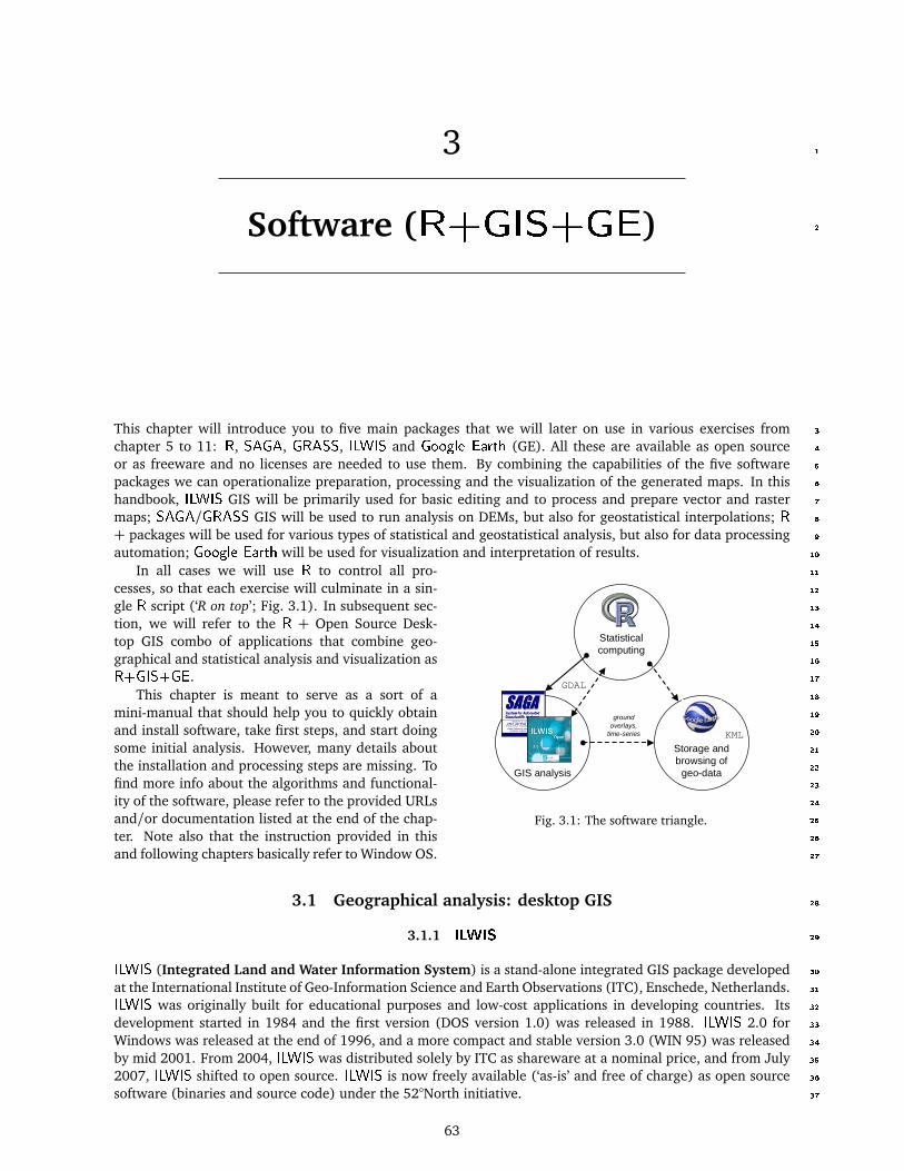
3 1
Software (R+GIS+GE) 2
This chapter will introduce you to five main packages that we will later on use in various exercises from 3
chapter 5 to 11: R, SAGA, GRASS, ILWIS and Google Earth (GE). All these are available as open source 4
or as freeware and no licenses are needed to use them. By combining the capabilities of the five software 5
packages we can operationalize preparation, processing and the visualization of the generated maps. In this 6
handbook, ILWIS GIS will be primarily used for basic editing and to process and prepare vector and raster 7
maps; SAGA/GRASS GIS will be used to run analysis on DEMs, but also for geostatistical interpolations; R 8
+ packages will be used for various types of statistical and geostatistical analysis, but also for data processing 9
automation; Google Earth will be used for visualization and interpretation of results. 10
GIS analysis
Storage andbrowsing of
geo-data
Statisticalcomputing
KML
GDAL
groundoverlays,
time-series
Fig. 3.1: The software triangle.
In all cases we will use R to control all pro- 11
cesses, so that each exercise will culminate in a sin- 12
gle R script (‘R on top’; Fig. 3.1). In subsequent sec- 13
tion, we will refer to the R + Open Source Desk- 14
top GIS combo of applications that combine geo- 15
graphical and statistical analysis and visualization as 16
R+GIS+GE. 17
This chapter is meant to serve as a sort of a 18
mini-manual that should help you to quickly obtain 19
and install software, take first steps, and start doing 20
some initial analysis. However, many details about 21
the installation and processing steps are missing. To 22
find more info about the algorithms and functional- 23
ity of the software, please refer to the provided URLs 24
and/or documentation listed at the end of the chap- 25
ter. Note also that the instruction provided in this 26
and following chapters basically refer to Window OS. 27
3.1 Geographical analysis: desktop GIS 28
3.1.1 ILWIS 29
ILWIS (Integrated Land and Water Information System) is a stand-alone integrated GIS package developed 30
at the International Institute of Geo-Information Science and Earth Observations (ITC), Enschede, Netherlands. 31
ILWIS was originally built for educational purposes and low-cost applications in developing countries. Its 32
development started in 1984 and the first version (DOS version 1.0) was released in 1988. ILWIS 2.0 for 33
Windows was released at the end of 1996, and a more compact and stable version 3.0 (WIN 95) was released 34
by mid 2001. From 2004, ILWIS was distributed solely by ITC as shareware at a nominal price, and from July 35
2007, ILWIS shifted to open source. ILWIS is now freely available (‘as-is’ and free of charge) as open source 36
software (binaries and source code) under the 52°North initiative. 37
63

64 Software (R+GIS+GE)
Fig. 3.2: ILWIS main window (above) and map window (below).
The most recent version of ILWIS1
(3.6) offers a range of image process-2
ing, vector, raster, geostatistical, statisti-3
cal, database and similar operations (Unit4
Geo Software Development, 2001). In ad-5
dition, a user can create new scripts, ad-6
just the operation menus and even build7
Visual Basic, Delphi, or C++ applications8
that will run on top of ILWIS and use9
its internal functions. In principle, the10
biggest advantage of ILWIS is that it is11
a compact package with a diverse vector12
and raster-based GIS functionality; the13
biggest disadvantages are bugs and insta-14
bilities and necessity to import data to IL-15
WIS format from other more popular GIS16
packages.17
To install ILWIS, download1 and run18
the MS Windows installation. In the19
installation folder, you will find the20
main executable for ILWIS. Double click21
this file to start ILWIS. You will first22
see the main program window, which23
can be compared to the ArcGIS catalog24
(Fig. 3.2). The main program window is,25
in fact, a file browser which lists all IL-26
WIS operations, objects and supplemen-27
tary files within a working directory. The28
ILWIS Main window consists of a Menu29
bar, a Standard toolbar, an Object selec-30
tion toolbar, a Command line, a Cata-31
log, a Status bar and an Operations/Nav-32
igator pane with an Operation-tree, an33
Operation-list and a Navigator. The left34
pane (Operations/Navigator) is used to35
browse available operations and directo-36
ries and the right menu shows available spatial objects and supplementary files (Fig. 3.2). GIS layers in37
different formats will not be visible in the catalog until we define the external file extension.38
An advantage of ILWIS is that, every time a user runs an command from the menu bar or operation tree,39
ILWIS will record the operation in ILWIS command language. For example, you can run ordinary kriging40
using: from the main menu select Operations 7→ Interpolation 7→ Point interpolation 7→ kriging, which will be41
shown as:42
ILWIS: log1p_zinc_OK.mpr = MapKrigingOrdinary(log1p_zinc, dist.grf,+ Exponential(0.000,0.770,449.000), 3000, plane, 0, 20, 60, no)
where log1p_zinc_OK.mpr is the output map, MapKrigingOrdinary is the interpolation function, log1p_zinc43
is the attribute point map with values of the target variable, dist.grf is the grid definition (georeference)44
and Exponential(0.000,0.770,449.000) are the variogram parameters (see also section 5.3.2). This means45
that you can now edit this command and run it directly from the command line, instead of manually selecting46
the operations from the menu bar. In addition, you can copy such commands into an ILWIS script to enable47
automation of data analysis. ILWIS script can use up to nine script parameters, which can be either spatial48
objects, values or textual strings.49
The new versions of ILWIS (>3.5) are developed as MS Visual 2008 project. The ILWIS user interface50
and ILWIS analytical functionality have now been completely separated making it easier to write server side51
1https://52north.org/download/Ilwis/

3.1 Geographical analysis: desktop GIS 65
applications for ILWIS. This allows us to control ILWIS also from R, e.g. by setting the location of ILWIS on 1
your machine: 2
> ILWIS <- "C:\\Progra∼1\\N52\\Ilwis35\\IlwisClient.exe -C"
To combine ILWIS and R commands in R, we use: 3
> shell(cmd=paste(ILWIS, "open log1p_zinc_OK.mpr -noask"), wait=F)
ILWIS has a number of built-in statistical and geostatistical functions. With respect to interpolation possi- 4
bilities, it can be used to prepare a variogram, to analyze the anisotropy in the data (including the variogram 5
surface), to run ordinary kriging and co-kriging (with one co-variable), to implement universal kriging with 6
coordinates2 as predictors and to run linear regression. ILWIS has also a number of original geostatistical 7
algorithms. For example, it offers direct kriging from raster data (which can be used e.g. to filter the missing 8
values in a raster map), and also does direct calculation of variograms from raster data. ILWIS is also suit- 9
able to run some basic statistical analysis on multiple raster layers (map lists): it offers principal component 10
analysis on rasters, correlation analysis between rasters and multi-layer map statistics (min, max, average and 11
standard deviation). 12
Fig. 3.3: Correlation plot dist vs log1p_zinc.
Although ILWIS cannot be used to run regression- 13
kriging as defined in §2.1.5, it can be used to run 14
a similar type of analysis. For example, a table 15
can be imported and converted to a point map us- 16
ing the Table to PointMap operation. The point 17
map can then be overlaid over raster maps to an- 18
alyze if the two variables are correlated. This can 19
be done by combining the table calculation and 20
the MapValue function. In the same table, you 21
can then derive a simple linear regression model 22
e.g. log1p_zinc = b0 + b1 * dist. By fitting a 23
least square fit using a polynomial, you will get: 24
b0=67.985 and b1=-4.429. This means that the zinc 25
concentration decreases with an increase of dist 26
— distance from the river (Fig. 3.3). Note that, 27
in ILWIS, you cannot derive the Generalized Least 28
Squares (GLS) regression coefficients (Eq.2.1.3) but 29
only the OLS coefficients, which is statistically sub- 30
optimal method, because the residuals are possibly 31
auto-correlated (see §2.1). In fact, regression mod- 32
eling in ILWIS is so limited that the best advice is to 33
always export the table data to R and then run statistical analysis using R packages. After estimating the 34
regression coefficients, you can produce a map of zinc content (deterministic part of variation) by running a 35
map calculation: 36
ILWIS: zinc_lm = 2.838 -1.169 * dist
Now you can estimate the residuals at sampled locations using table calculation: 37
ILWIS: log1p_zinc_res = log1p_zinc - MapValue(zinc_lm, coord(X,Y,NL_RD))
You can create a point map for residuals and derive a variogram of residuals by using operations Statistics 38
7→ Spatial correlation from the main menu. If you use a lag spacing of 100 m, you will get a variogram that 39
can be fitted3 with an exponential variogram model (C0=0.008, C1=0.056, R=295). The residuals can now be 40
interpolated using ordinary kriging, which produces a typical kriging pattern. The fitted trend and residuals 41
can then be added back together using: 42
2In ILWIS, the term Universal kriging is used exclusively for interpolation of point data using transforms of the coordinates.3ILWIS does not support automated variogram fitting.

66 Software (R+GIS+GE)
ILWIS: zinc_res_OK.mpr = MapKrigingOrdinary(log1p_zinc_res, dist.grf,+ Exponential(0.008,0.056,295.000), 3000, plane, 0, 20, 60, no)ILWIS: log1p_zinc_RK = zinc_lm + zinc_res_OKILWIS: zinc_rk = pow(10, log1p_zinc_RK)-1
which gives regression-kriging predictions. Note that, because a complete RK algorithm with GLS estimation1
of regression is not implemented in ILWIS (§2.1.5), we are not able to derive a map of the prediction variance2
(Eq.2.1.5). For these reasons, regression-kriging in ILWIS is not really encouraged and you should consider3
using more sophisticated geostatistical packages such as gstat and/or geoR.4
Finally, raster maps from ILWIS can be exported to other packages. You can always export them to ArcInfo5
ASCII (.ASC) format. If the georeference in ILWIS has been set as center of the corner pixels, then you might6
need to manually edit the *.asc header4. Otherwise, you will not be able to import such maps to ArcGIS (87
or higher) or e.g. Idrisi. The pending ILWIS v3.7 will be even more compatible with the OGC simple features,8
WPS query features and similar. At the moment, the fastest and most efficient solution to read/write ILWIS9
rasters to other supported GDAL formats is FWTools5.10
3.1.2 SAGA11
SAGA6 (System for Automated Geoscientific Analyzes) is an open source GIS that has been developed since12
2001 at the University of Göttingen7, Germany, with the aim to simplify the implementation of new algorithms13
for spatial data analysis (Conrad, 2006, 2007). It is a full-fledged GIS with support for raster and vector data.14
SAGA includes a large set of geoscientific algorithms, and is especially powerful for the analysis of DEMs.15
With the release of version 2.0 in 2005, SAGA runs under both Windows and Linux operating systems. SAGA16
is an open-source package, which makes it especially attractive to users that would like to extend or improve17
its existing functionality.18
Fig. 3.4: The SAGA GUI elements and displays.
SAGA handles tables, vector and raster data and natively supports at least one file format for each data19
type. Currently SAGA (2.0.4) provides about 48 free module libraries with >300 modules, most of them20
4Simply replace in the header of the file xllcenter and yllcenter with xllcorner and yllcorner.5http://fwtools.maptools.org6http://saga-gis.org7The group recently collectively moved to the Institut für Geographie, University of Hamburg.

3.1 Geographical analysis: desktop GIS 67
published under the GPL. The modules cover geo–statistics, geomorphometric analysis, image processing, 1
cartographic projections, and various tools for vector and raster data manipulation. Modules can be executed 2
directly by using their associated parameters window. After you have imported all maps to SAGA, you can 3
also save the whole project so that all associated maps and visualization settings are retained. The most 4
comprehensive modules in SAGA are connected with hydrologic, morphometric and climatic analysis of DEMs. 5
To install SAGA, download and unzip the compiled binaries8 to some default local directory. Then run 6
the saga_gui.exe and you will get a GUI as shown in Fig. 3.4. Likewise, to install SAGA on Linux machines, 7
you can also download the compiled binaries (e.g. saga_2.0.4_bin_linux.tar.gz), then run some basic 8
configuration: 9
> ./configure --enable-unicode --with-gnu-ld=yes
Note that there are two possibilities to compile the software under Linux: (a) either a Non-Unicode or (b) 10
a Unicode version of SAGA. Building the Unicode version is straight forward and recommended. Have also 11
in mind that, under Linux, wxWidgets, PROJ 4, GDAL, JASPER, TIFF and GCC packages need to be obtained 12
and configured separately before you can start using SAGA (for the unicode compilation, wx. configure does 13
not check for JASPER libraries!). For a correct installation, you should follow the instructions provided via the 14
SAGA WIKI9. SAGA is unfortunately still not available for Mac OS X. 15
In addition to the GUI, a second user front end, the SAGA command line interpreter can be used to 16
execute modules. Library RSAGA10 provides access to geocomputing and terrain analysis functions of SAGA 17
from within R by running the command line version of SAGA (Brenning, 2008)11. RSAGA provides also 18
several R functions for handling and manipulating ASCII grids, including a flexible framework for applying 19
local functions or focal functions to multiple grids (Brenning, 2008). It is important to emphasize that RSAGA 20
package is used mainly to control SAGA operations from R. To be able to run RSAGA, you need to have SAGA 21
installed locally on your machine. SAGA GIS does NOT come in the RSAGA library. 22
To find what SAGA libraries12 and modules do and require, you should use the rsaga.get.modules and 23
rsaga.get.usage commands. For example, to see which parameters are needed to generate a DEM from a 24
shapefile type: 25
> rsaga.env()
$workspace[1] "."
$cmd[1] "saga_cmd.exe"
$path[1] "C:/Progra∼1/saga_vc"
$modules[1] "C:/Progra∼1/saga_vc/modules"
> rsaga.get.modules("grid_spline")
$grid_splinecode name interactive
1 0 Thin Plate Spline (Global) FALSE2 1 Thin Plate Spline (Local) FALSE3 2 Thin Plate Spline (TIN) FALSE4 3 B-Spline Approximation FALSE5 4 Multilevel B-Spline Interpolation FALSE6 5 Multilevel B-Spline Interpolation (from Grid) FALSE7 NA <NA> FALSE8 NA <NA> FALSE
8http://sourceforge.net/projects/saga-gis/files/9http://sourceforge.net/apps/trac/saga-gis/wiki/CompilingaLinuxUnicodeversion
10http://cran.r-project.org/web/packages/RSAGA/11RPyGeo package can be used to control ArcGIS geoprocessor in a similar way.12We also advise you to open SAGA and then first run processing manually (point–and–click) processing. The names of the SAGA
libraries can be obtained by browsing the /modules/ directory.
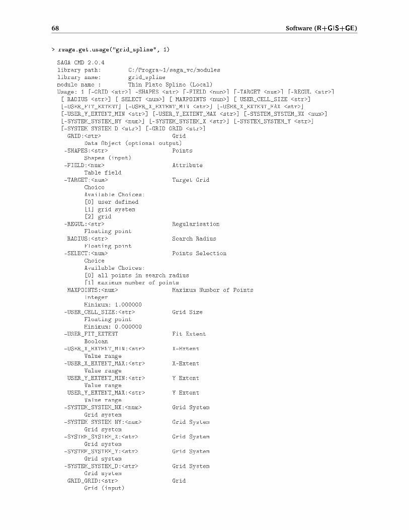
68 Software (R+GIS+GE)
> rsaga.get.usage("grid_spline", 1)
SAGA CMD 2.0.4library path: C:/Progra∼1/saga_vc/moduleslibrary name: grid_splinemodule name : Thin Plate Spline (Local)Usage: 1 [-GRID <str>] -SHAPES <str> [-FIELD <num>] [-TARGET <num>] [-REGUL <str>][-RADIUS <str>] [-SELECT <num>] [-MAXPOINTS <num>] [-USER_CELL_SIZE <str>][-USER_FIT_EXTENT] [-USER_X_EXTENT_MIN <str>] [-USER_X_EXTENT_MAX <str>][-USER_Y_EXTENT_MIN <str>] [-USER_Y_EXTENT_MAX <str>] [-SYSTEM_SYSTEM_NX <num>][-SYSTEM_SYSTEM_NY <num>] [-SYSTEM_SYSTEM_X <str>] [-SYSTEM_SYSTEM_Y <str>][-SYSTEM_SYSTEM_D <str>] [-GRID_GRID <str>]-GRID:<str> Grid
Data Object (optional output)-SHAPES:<str> Points
Shapes (input)-FIELD:<num> Attribute
Table field-TARGET:<num> Target Grid
ChoiceAvailable Choices:[0] user defined[1] grid system[2] grid
-REGUL:<str> RegularisationFloating point
-RADIUS:<str> Search RadiusFloating point
-SELECT:<num> Points SelectionChoiceAvailable Choices:[0] all points in search radius[1] maximum number of points
-MAXPOINTS:<num> Maximum Number of PointsIntegerMinimum: 1.000000
-USER_CELL_SIZE:<str> Grid SizeFloating pointMinimum: 0.000000
-USER_FIT_EXTENT Fit ExtentBoolean
-USER_X_EXTENT_MIN:<str> X-ExtentValue range
-USER_X_EXTENT_MAX:<str> X-ExtentValue range
-USER_Y_EXTENT_MIN:<str> Y-ExtentValue range
-USER_Y_EXTENT_MAX:<str> Y-ExtentValue range
-SYSTEM_SYSTEM_NX:<num> Grid SystemGrid system
-SYSTEM_SYSTEM_NY:<num> Grid SystemGrid system
-SYSTEM_SYSTEM_X:<str> Grid SystemGrid system
-SYSTEM_SYSTEM_Y:<str> Grid SystemGrid system
-SYSTEM_SYSTEM_D:<str> Grid SystemGrid system
-GRID_GRID:<str> GridGrid (input)

3.1 Geographical analysis: desktop GIS 69
Most SAGA modules — with the exception of a few that can only be executed in interactive mode — can be 1
run from within R using the rsaga.geoprocessor function, RSAGA’s low-level workhorse. However, RSAGA 2
also provides R wrapper functions and associated help pages for many SAGA modules. As an example, a slope 3
raster can be calculated from a digital elevation model with SAGA’s local morphometry module, which can 4
be accessed with the rsaga.local.morphometry function or more specifically with rsaga.slope (Brenning, 5
2008). 6
SAGA can read directly ESRI shapefiles and table data. Grids need to be converted to the native SAGA 7
grid format (*.sgrd). This raster format is now supported by GDAL (starting with GDAL 1.7.0) and can be 8
read directly via the readGDAL method. Alternatively, you can convert some GDAL-supported formats to SAGA 9
grids and back by using: 10
# write to SAGA grid:> rsaga.esri.to.sgrd(in.grids="meuse_soil.asc", out.sgrd="meuse_soil.sgrd",+ in.path=getwd())# read SAGA grid:> rsaga.sgrd.to.esri(in.sgrd="meuse_soil.sgrd", out.grids="meuse_soil.asc",+ out.path=getwd())
SAGA grid comprises tree files: 11
(1.) *.sgrd — the header file with name, data format, XLL, YLL, rows columns, cell size, z-factor and no 12
data value; 13
(2.) *.sdat - the raw data file; 14
(3.) *.hgrd - the history file; 15
In some cases, you might consider reading directly the raw data and header data to R, which can be done 16
by using e.g.: 17
# read SAGA grid format:> sgrd <- matrix((unlist(strsplit(readLines(file("meuse_soil.sgrd")), split="\t= "))),+ ncol=2, byrow=T)> sgrd
[,1] [,2][1,] "NAME" "meuse_soil"[2,] "DESCRIPTION" "UNIT"[3,] "DATAFILE_OFFSET" "0"[4,] "DATAFORMAT" "FLOAT"[5,] "BYTEORDER_BIG" "FALSE"[6,] "POSITION_XMIN" "178460.0000000000"[7,] "POSITION_YMIN" "329620.0000000000"[8,] "CELLCOUNT_X" "78"[9,] "CELLCOUNT_Y" "104"[10,] "CELLSIZE" "40.0000000000"[11,] "Z_FACTOR" "1.000000"[12,] "NODATA_VALUE" "-9999.000000"[13,] "TOPTOBOTTOM" "FALSE"
# read the raw data: 4bit, numeric (FLOAT), byte order small;> sdat <- readBin("meuse_soil.sdat", what="numeric", size=4,+ n=as.integer(sgrd[8,2])*as.integer(sgrd[9,2]))> sdat.sp <- as.im(list(x=seq(from=as.integer(sgrd[6,2]),+ length.out=as.integer(sgrd[8,2]), by=as.integer(sgrd[10,2])),+ y=seq(from=as.integer(sgrd[7,2]), length.out=as.integer(sgrd[9,2]),+ by=as.integer(sgrd[10,2])), z=matrix(sdat, nrow=as.integer(sgrd[8,2]),+ ncol=as.integer(sgrd[9,2]))))> sdat.sp <- as(sdat.sp, "SpatialGridDataFrame")# replace the mask value with NA's:> sdat.sp@data[[1]] <- ifelse(sdat.sp@data[[1]]==as.integer(sgrd[12,2]), NA,+ sdat.sp@data[[1]])> spplot(sdat.sp)

70 Software (R+GIS+GE)
Another possibility to read SAGA grids directly to R is via the read.sgrd wrapper function (this uses1
rsaga.sgrd.to.esri method to write to a tempfile()), and then read.ascii.grid to import data to R):2
> gridmaps <- readGDAL("meuse_soil.asc")> gridmaps$soil <- as.vector(t(read.sgrd("meuse_soil.sgrd", return.header=FALSE)))
which reads raw data as a vector to an existing SpatialGridDataFrame.3
SAGA offers limited capabilities for geostatistical analysis, but in a very user-friendly environment. Note4
that many commands in SAGA are available only by right-clicking the specific data layers. For example, you5
can make a correlation plot between two grids by right-clicking a map of interest, then select Show Scatterplot6
and you will receive a module execution window where you can select the second grid (or a shapefile) that you7
would like to correlate with your grid of interest. This will plot all grid-pairs and display the regression model8
and its R-square (see further Fig. 10.8). The setting of the Scatterplot options can be modified by selecting9
Scatterplot from the main menu. Here you can adjust the regression formula, obtain the regression details,10
and adjust the graphical settings of the scatterplot.11
Under the module Geostatistics, three groups of operations can be found: (a) Grid (various operations12
on grids); (b) Points (derivation of semivariances) and (c) Kriging (ordinary and universal kriging). Under13
the group Grid, several modules can be run: Multiple Regression Analysis (relates point data with rasters),14
Radius of Variance (detects a minimum radius to reach a particular variance value in a given neighborhood),15
Representativeness (derives variance in a local neighborhood), Residual Analysis (derives local mean value,16
local difference from mean, local variance, range and percentile), Statistics for Grids (derives mean, range17
and standard deviation for a list of rasters) and Zonal Grid Statistics (derives statistical measures for various18
zones and based on multiple grids). For the purpose of geostatistical mapping, we are especially interested19
in correlating points with rasters (see §1.3.2), which can be done via the Multiple Regression Analysis module.20
Initiating this module opens a parameter setting window (Fig. 3.5).21
In the Multiple Regression Analysis module, SAGA will estimate the values of points at grids, run the22
regression analysis and predict the values at each location. You will also get a textual output (message window)23
that will show the regression model, and a list of the predictors according to their importance e.g.:24
Executing module: Multiple Regression Analysis (Grids/Points)ParametersGrid system: 40; 78x 104y; 178460x 329620yGrids: 2 objects (dist, ahn))Shapes: zinc.shpAttribute: log1p_zincDetails: Multiple Regression AnalysisResiduals: zinc.shp [Residuals]Regression: zinc.shp (Multiple Regression Analysis (Grids/Points))Grid Interpolation: B-Spline Interpolation
Regression:Y = 6.651112 -2.474725*[dist] -0.116471*[ahn]
Correlation:1: R2 = 54.695052% [54.695052%] -> dist2: R2 = 55.268255% [0.573202%] -> ahn
in this case the most significant predictor is dist; the second predictor explains <1% of the variability in25
log1p_zinc (see further Fig. 5.6). The model explains 55.3% of the total variation.26
When selecting the multiple regression analysis options, you can also opt to derive the residuals and fit27
the variogram of residuals. These will be written as a shapefile that can then be used to derive semivari-28
ances. Select Geostatistics 7→ Points 7→ Semivariogram and specify the distance increment (lag) and maximum29
distance. The variogram can be displayed by again right clicking a table and selecting Show Scatterplot op-30
tion. Presently, the variogram (regression) models in SAGA are limited to linear, exponential and logarithmic31
models. In general, fitting and use of variograms in SAGA is discouraged13.32
13Exceptionally, you should use the logarithmic model which will estimate something close to the exponential variogram model(Eq.1.3.8).

3.1 Geographical analysis: desktop GIS 71
Fig. 3.5: Running predictions by using regression analysis in SAGA GIS: parameter settings window. The “Grid Interpola-tion” setting indicates the way SAGA will estimate values of grids at calibration points. This should not be confused withother gridding techniques available in SAGA.
Once the regression model and the variogram of the residuals have been estimated, a user can also run 1
regression-kriging, which is available in SAGA under the module Geostatistics 7→ Universal kriging. Global and 2
local (search radius) version of the Universal kriging are available. Use of local Universal kriging with a small 3
search radius (�100 points) is not recommended because it over-simplifies the technique, and can lead to 4
artefacts14. Note also that, in SAGA, you can select as many predictors as you wish, as long as they are all in 5
the same grid system. The final results can be visualized in both 2D and 3D spaces. 6
Another advantage of SAGA is the ability to use script files for the automation of complex work-flows, 7
which can then be applied to different data projects. Scripting of SAGA modules is now possible in two ways: 8
(1.) Using the command line interpreter (saga_cmd.exe) with DOS batch scripts. Some instructions on how 9
to generate batch files can be found in Conrad (2006, 2007). 10
(2.) A much more flexible way of scripting utilizes the Python interface to the SAGA Application Program- 11
ming Interface (SAGA-API). 12
In addition to scripting possibilities, SAGA allows you to save SAGA parameter files (*.sprm) that contain 13
all inputs and output parameters set using the module execution window. These parameter files can be edited 14
in an ASCII editor, which can be quite useful to automate processing. 15
In summary, SAGA GIS has many attractive features for both geographical and statistical analysis of spatial 16
data: (1) it has a large library of modules, especially to parameterize geomorphometric features, (2) it can 17
generate maps from points and rasters by using multiple linear regression and regression-kriging, and (3) it is 18
an open source GIS with a popular GUI. Compared to gstat, SAGA is not able to run geostatistical simulations, 19
GLS estimation nor stratified or co-kriging. However, it is capable of running regression-kriging in a statistically 20
sound way (unlike ILWIS). The advantage of SAGA over R is that it can load and process relatively large maps 21
(not recommended in R for example) and that it can be used to visualize the input and output maps in 2D and 22
2.5D (see further section 5.5.2). 23
3.1.3 GRASS GIS 24
GRASS15 (Geographic Resources Analysis Support System) is a general-purpose Geographic Information 25
System (GIS) for the management, processing, analysis, modeling and visualization of many types of geo- 26
referenced data. It is Open Source software released under GNU General Public License and is available on 27
14Neither local variograms nor local regression models are estimated. See §2.2 for a detailed discussion.15http://grass.itc.it

72 Software (R+GIS+GE)
the three major platforms (Microsfot Windows, Mac OS X and Linux). The main component of the develop-1
ment and software maintenance is built on top of highly automated web-based infrastructure sponsored by2
ITC-irst (Centre for Scientific and Technological Research) in Trento, Italy with numerous worldwide mirror3
sites. GRASS includes functions to process raster maps, including derivation of descriptive statistics for maps,4
histograms, but also generation of statistics for time series. There are also several unique interpolation tech-5
niques. For example the Regularized Spline with Tension (RST) interpolation, which has been quoted as one6
of the most sophisticated methods to generate smooth surfaces from point data (Mitasova et al., 2005).7
In version 5.0 of GRASS, several basic geostatistical functionalities existed including ordinary kriging and8
variogram plotting, however, developers of GRASS ultimately concluded that there was no need to build9
geostatistical functionality from scratch when a complete open source package already existed. The current10
philosophy (v 6.5) focuses on making GRASS functions also available in R, so that both GIS and statistical11
operations can be integrated in a single command line. A complete overview of the Geostatistics and spatial12
data analysis functionality can be found via the GRASS website16. Certainly, if you are a Linux user and13
already familiar with GRASS, you will probably not encounter many problems in installing GRASS and using14
the syntax.15
Unlike SAGA, GRASS requires that you set some initial ‘environmental’ parameters, i.e. initial setting that16
describe your project. There are three initial environmental parameters: DATABASE — a directory (folder)17
on disk to contain all GRASS maps and data; LOCATION — the name of a geographic location (defined by18
a co-ordinate system and a rectangular boundary), and MAPSET — a rectangular REGION and a set of maps19
(Neteler and Mitasova, 2008). Every LOCATION contains at least a MAPSET called PERMANENT, which is read-20
able by all sessions. GRASS locations are actually powerful abstractions that do resemble the way in which21
workflows were/are set up in larger multi-user projects. The mapsets parameter is used to distinguish users,22
and PERMANENT was privileged with regard to who could change it — often the database/location/mapset tree23
components can be on different physical file systems. On single-user systems or projects, this construction24
seems irrelevant, but it isn’t when many users work collaborating on the same location.25
GRASS can be controlled from R thanks to the spgrass617 package (Bivand, 2005; Bivand et al., 2008):26
initGRASS can be used to define the environmental parameters; description of each GRASS module can be27
obtained by using the parseGRASS method. The recommended reference manual for GRASS is the “GRASS28
book” (Neteler and Mitasova, 2008); a complete list of the modules can be found in the GRASS reference29
manual18. Some examples of how to use GRASS via R are shown in §10.6.2. Another powerful combo of30
applications similar to the one shown in Fig. 3.1 is the QGIS+GRASS+R triangle. In this case, a GUI (QGIS)31
stands on top of GRASS (which stands on top of R), so that this combination is worth checking for users that32
prefer GUI’s.33
3.2 Statistical computing: R34
R19 is the open source implementation of the S language for statistical computing (R Development Core Team,35
2009). Apparently, the name “R” was selected for two reasons: (1) precedence — “R” is a letter before36
“S”, and (2) coincidence — both of the creators’ names start with a letter “R”. The S language provides37
a wide variety of statistical (linear and nonlinear modeling, classical statistical tests, time-series analysis,38
classification, clustering,. . . ) and graphical techniques, and is highly extensible (Chambers and Hastie, 1992;39
Venables and Ripley, 2002). It has often been the vehicle of choice for research in statistical methodology, and40
R provides an Open Source route to participation in that activity.41
Although much of the R code is always under development, a large part of the code is usable, portable and42
extendible. This makes R one of the most suitable coding environments for academic societies. Although it43
typically takes a lot of time for non-computer scientists to learn the R syntax, the benefits are worth the time44
investment.45
To install R under Windows, download and run an installation executable file from the R-project homepage.46
This will install R for Windows with a GUI. After starting R, you will first need to set-up the working directory47
and install additional packages. To run geostatistical analysis in R, you will need to add the following R48
packages: gstat (gtat in R), rgdal (GDAL import of GIS layers in R), sp (support for spatial objects in R),49
16http://grass.itc.it/statsgrass/17http://cran.r-project.org/web/packages/spgrass6/18See your local installation file:///C:/GRASS/docs/html/full_index.html.19http://www.r-project.org
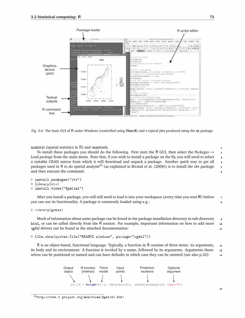
3.2 Statistical computing: R 73
Fig. 3.6: The basic GUI of R under Windows (controlled using Tinn-R) and a typical plot produced using the sp package.
spatstat (spatial statistics in R) and maptools. 1
To install these packages you should do the following. First start the R GUI, then select the Packages 7→ 2
Load package from the main menu. Note that, if you wish to install a package on the fly, you will need to select 3
a suitable CRAN mirror from which it will download and unpack a package. Another quick way to get all 4
packages used in R to do spatial analysis20 (as explained in Bivand et al. (2008)) is to install the ctv package 5
and then execute the command: 6
> install.packages("ctv")> library(ctv)> install.views("Spatial")
After you install a package, you will still need to load it into your workspace (every time you start R) before 7
you can use its functionality. A package is commonly loaded using e.g.: 8
> library(gstat)
Much of information about some package can be found in the package installation directory in sub-directory 9
html, or can be called directly from the R session. For example, important information on how to add more 10
rgdal drivers can be found in the attached documentation: 11
> file.show(system.file("README.windows", package="rgdal"))
R is an object-based, functional language. Typically, a function in R consists of three items: its arguments, 12
its body and its environment. A function is invoked by a name, followed by its arguments. Arguments them- 13
selves can be positional or named and can have defaults in which case they can be omitted (see also p.32): 14
15
20http://cran.r-project.org/web/views/Spatial.html

74 Software (R+GIS+GE)
Functions typically return their result as their value, not via an argument. In fact, if the body of a function1
changes an argument it is only changing a local copy of the argument and the calling program does not get2
the changed result.3
R is widely recognized as one of the fastest growing and most comprehensive statistical computing tools21.4
It is estimated that the current number of active R users (Google trends service) is about 430k, but this number5
is constantly growing. R practically offers statistical analysis and visualization of unlimited sophistication. A6
user is not restricted to a small set of procedures or options, and because of the contributed packages, users7
are not limited to one method of accomplishing a given computation or graphical presentation. As we will see8
later, R became attractive for geostatistical mapping mainly due to the recent integration of the geostatistical9
tools (gstat, geoR) and tools that allow R computations with spatial data layers (sp, maptools, raster and10
similar).11
Note that in R, the user must type commands to enter data, do analyzes, and plot graphs. This might seem12
inefficient to users familiar with MS Excel and similar intuitive, point-and-click packages. If a single argument13
in the command is incorrect, inappropriate or mistyped, you will get an error message indicating where the14
problem might be. If the error message is not helpful, then try receiving more help about some operation.15
Many very useful introductory notes and books, including translations of manuals into other languages than16
English, are available from the documentation section22. Another very useful source of information is the17
R News23 newsletter, which often offers many practical examples of data processing. Vol. 1/2 of R News,18
for example, is completely dedicated to spatial statistics in R; see also Pebesma and Bivand (2005) for an19
overview of classes and methods for spatial data in R. The ‘Spatial’ packages can be nicely combined with20
e.g. the ‘Environmentrics’24 packages. The interactive graphics25 in R is also increasingly powerful (Urbanek21
and Theus, 2008). To really get an idea about the recent developments, and to get support with using spatial22
packages, you should register with the special interest group R-sig-Geo26.23
Although there are several packages in R to do geostatistical analysis and mapping, many recognize24
R+gstat/geoR as the only complete and fully-operational packages, especially if you wish to run regression-25
kriging, multivariate analysis, geostatistical simulations and block predictions (Hengl et al., 2007a; Rossiter,26
2007). To allow extension of R functionalities to operations with spatial data, the developer of gstat, with27
the support of colleagues, has developed the sp27 package (Pebesma and Bivand, 2005; Bivand et al., 2008).28
Now, users are able to load GIS layers directly into R, run geostatistical analysis on grid and points and display29
spatial layers as in a standard GIS package. In addition to sp, two important spatial data protocols have also30
been recently integrated into R: (1) GIS data exchange protocols (GDAL — Geospatial Data Abstraction Li-31
brary, and OGR28 — OpenGIS Simple Features Reference Implementation), and (2) map projection protocols32
(PROJ.429 — Cartographic Projections Library). These allow R users to import/export raster and vector maps,33
run raster/vector based operations and combine them with statistical computing functionality of various pack-34
ages. The development of GIS and graphical functionalities within R has already caused a small revolution35
and many GIS analysts are seriously thinking about completely shifting to R.36
3.2.1 gstat37
gstat30 is a stand-alone package for geostatistical analysis developed by Edzer Pebesma during his PhD studies38
at the University of Utrecht in the Netherlands in 1997. As of 2003, the gstat functionality is also available39
as an S extension, either as R package or S-Plus library. Current development focuses mainly on the R/S40
extensions, although the stand alone version can still be used for many applications. To install gstat (the41
stand-alone version) under Windows, download the gstat.exe and gstatw.exe (variogram modeling with42
GUI) files from the gstat.org website and put them in your system directory31. Then, you can always run gstat43
from the Windows start menu. The gstat.exe runs as a DOS application, which means that there is no GUI.44
21The article in the New Your Times by Vance (2009) has caused much attention.22http://www.r-project.org/doc/bib/R-books.html23http://cran.r-project.org/doc/Rnews/; now superseded by R Journal.24http://cran.r-project.org/web/views/Environmetrics.html25http://www.interactivegraphics.org26https://stat.ethz.ch/mailman/listinfo/r-sig-geo27http://r-spatial.sourceforge.net28http://www.gdal.org/ogr/ — for Mac OS X users, there is no binary package available from CRAN.29http://proj.maptools.org30http://www.gstat.org31E.g. C:\Windows\system32\

3.2 Statistical computing: R 75
A user controls the processing by editing the command files. 1
gstat is possibly the most complete, and certainly the most accessible geostatistical package in the World. 2
It can be used to calculate sample variograms, fit valid models, plot variograms, calculate (pseudo) cross 3
variograms, and calculate and fit directional variograms and variogram models (anisotropy coefficients are 4
not fitted automatically). Kriging and (sequential) conditional simulation can be done under (simplifications 5
of) the universal co-kriging model. Any number of variables may be spatially cross-correlated. Each variable 6
may have its own number of trend functions specified (being coordinates, or so-called external drift variables). 7
Simplifications of this model include ordinary and simple kriging, ordinary or simple co-kriging, universal 8
kriging, external drift kriging, Gaussian conditional or unconditional simulation or cosimulation. In addition, 9
variables may share trend coefficients (e.g. for collocated co-kriging). To learn about capabilities of gstat, a 10
user is advised to read the gstat User’s manual32, which is still by far the most complete documentation of the 11
gstat. 12
A complete overview of gstat functions and examples of R commands are given in Pebesma (2004). A 13
more recent update of the functionality can be found in Bivand et al. (2008, §8); gstat development tree is 14
from 2010 also available from a public SVN33. The most widely used gstat functions in R include: 15
variogram — calculates sample (experimental) variograms; 16
plot.variogram — plots an experimental variogram with automatic detection of lag spacing and maxi- 17
mum distance; 18
fit.variogram — iteratively fits an experimental variogram using reweighted least squares estimation; 19
krige — a generic function to make predictions by inverse distance interpolation, ordinary kriging, OLS 20
regression, regression-kriging and co-kriging; 21
krige.cv — runs krige with cross-validation using the n-fold or leave-one-out method; 22
R offers much more flexibility than the stand-alone version of gstat, because users can extend the optional 23
arguments and combine them with outputs or functions derived from other R packages. For example, instead 24
of using a trend model with a constant (intercept), one could use outputs of a linear model fitting, which 25
allows even more compact scripting. 26
3.2.2 The stand-alone version of gstat 27
As mentioned previously, gstat can be run as a stand-alone application, or as a R package. In the stand- 28
alone version of the gstat, everything is done via compact scripts or command files. The best approach to 29
prepare the command files is to learn from the list of example command files that can be found in the gstat 30
User’s manual34. Preparing the command files for gstat is rather simple and fast. For example, to run inverse 31
distance interpolation the command file would look like this: 32
# Inverse distance interpolation on a mask map
data(zinc): 'meuse.eas', x=1, y=2, v=3;mask: 'dist.asc'; # the prediction locationspredictions(zinc): 'zinc_idw.asc'; # result map
where the first line defines the input point data set (points.eas — an input table in the GeoEAS35 format), 33
the coordinate columns (x , y) are the first and the second column in this table, and the variable of interest 34
is in the third column; the prediction locations are the grid nodes of the map dist.asc36 and the results of 35
interpolation will be written to a raster map zinc_idw.asc. 36
To extend the predictions to regression-kriging, the command file needs to include the auxiliary maps and 37
the variogram model for the residuals: 38
32http://gstat.org/manual/33https://52north.org/svn/geostatistics/34http://gstat.org/manual/node30.html35http://www.epa.gov/ada/csmos/models/geoeas.html36Typically ArcInfo ASCII format for raster maps.

76 Software (R+GIS+GE)
# Regression-kriging using two auxiliary maps# Target variable is log-transformed
data(ln_zinc): 'meuse.eas', x=1, y=2, v=3, X=4,5, log;variogram(ln_zinc): 0.055 Nug(0) + 0.156 Exp(374);mask: 'dist.asc', 'ahn.asc'; # the predictorspredictions(ev): 'ln_zinc_rk.asc'; # result map
where X defines the auxiliary predictors, 0.055 Nug(0) + 0.156 Exp(374) is the variogram of residuals and1
dist.asc and ahn.asc are the auxiliary predictors. All auxiliary maps need to have the same grid definition2
and need to be available also in the input table. In addition, the predictors need to be sorted in the same order3
in both the first and the third line. Note that there are many optional arguments that can be included in the4
command file: a search radius can be set using "max=50"; switching from predictions to simulations can be5
done using "method: gs"; bloc kriging can be initiated using "blocksize: dx=100".6
To run a command file start DOS prompt by typing: > cmd, then move to the active directory by typing:7
e.g. > cd c:\gstat; to run spatial predictions or simulations run the gstat program together with a specific8
gstat command file from the Windows cmd console (Fig. 3.7):9
cmd gstat.exe ec1t.cmd
Fig. 3.7: Running interpolation using the gstat stand-alone: the DOS command prompt.
gstat can also automatically fit a variogram by using:10
data(ev): 'points.eas', x=1,y=2,v=3;
# set an initial variogram:variogram(ev): 1 Nug(0) + 5 Exp(1000);# fit the variogram using standard weights:method: semivariogram;set fit=7;
# write the fitted variogram model and the corresponding gnuplotset output= 'vgm_ev.cmd';set plotfile= 'vgm_ev.plt';
where set fit=7 defines the fitting method (weights=N j/h2j ), vgm_ev.cmd is the text file where the fitted11
parameters will be written. Once you fitted a variogram, you can then view it using the wgnuplot37. Note that,12
for automated modeling of variogram, you will need to define the fitting method and an initial variogram,13
which is then iteratively fitted against the sampled values. A reasonable initial exponential variogram can be14
37http://www.gnuplot.info

3.2 Statistical computing: R 77
produced by setting nugget parameter = measurement error, sill parameter = sampled variance, and range 1
parameter = 10% of the spatial extent of the data (or two times the mean distance to the nearest neighbor). 2
This can be termed a standard initial variogram model. Although the true variogram can be quite different, 3
it is important to have a good idea of what the variogram should look like. 4
There are many advantages to using the stand-alone version of gstat. The biggest ones are that it takes little 5
time to prepare a script and that it can work with large maps (unlike R that often faces memory problems). In 6
addition, the results of interpolation are directly saved in a GIS format and can be loaded to ILWIS or SAGA. 7
However, for regression-kriging, we need to estimate the regression model first, then derive the residuals and 8
estimate their variogram model, which cannot be automated in gstat so we must in any case load the data to 9
some statistical package before we can prepare the command file. Hence, the stand-alone version of gstat, as 10
with SAGA, can be used for geostatistical mapping only after regression modeling and variogram fitting have 11
been completed. 12
3.2.3 geoR 13
An equally comprehensive package for geostatistical analysis is geoR, a package extensively described by 14
Diggle and Ribeiro Jr (2007) and Ribeiro Jr et al. (2003); a series of tutorials can be found on the package 15
homepage38. In principle, a large part of the functionality of gstat and geoR overlap39; on the other hand, 16
geoR has many original methods, including an original format for spatial data (called geodata). geoR can be 17
in general considered to be more suited for variogram model estimation (including interactive visual fitting), 18
modeling of non-normal variables and simulations. A short demo of what geoR can do considering standard 19
geostatistical analysis is given in section 5.5.3. 20
geoR also allows for Bayesian kriging; its extension — the package geoRglm — can work with binomial 21
and Poisson processes (Ribeiro Jr et al., 2003). In comparison, fitting a Generalized Linear Geostatistical 22
Model (GLGM) can be more conclusive than fitting simple linear models in gstat since we can model the 23
geographical and regression terms more objectively (Diggle and Ribeiro Jr, 2007). This was, for example, the 24
original motivation for the geoRglm and spBayes packages (Ribeiro Jr et al., 2003). However, GLGMs are not 25
yet ready for operational mapping, and R code will need to be adapted. 26
3.2.4 Isatis 27
Fig. 3.8: Exploratory data analysis possibilities in Isatis.
Isatis40 is probably the most expensive geo- 28
statistical package (>10K €) available on the 29
market today. However, it is widely regarded 30
as one of the most professional packages for 31
environmental sciences. Isatis was originally 32
built for Unix, but there are MS Windows and 33
Linux versions also. From the launch of the 34
package in 1993, >1000 licences have been 35
purchased worldwide. Standard Isatis clients 36
are Oil and Gas companies, consultancy teams, 37
mining corporations and environmental agen- 38
cies. The software will be here shortly pre- 39
sented for informative purposes. We will not 40
use Isatis in the exercises, but it is worth men- 41
tioning it. 42
Isatis offers a wide range of geostatistical 43
functions ranging from 2D/3D isotropic and di- 44
rectional variogram modeling, univariate and 45
multivariate kriging, punctual and block esti- 46
mation, drift estimation, universal kriging, col- 47
38http://www.leg.ufpr.br/geoR/geoRdoc/tutorials.html39Other comparable packages with geostatistical analysis are �elds, spatial, sgeostat and RandomFields, but this book for practical
reasons focuses only on gstat and geoR.40http://www.geovariances.com — the name “Isatis” is not an abbreviation. Apparently, the creators of Isatis were passionate
climbers so they name their package after one climbing site in France.

78 Software (R+GIS+GE)
located co-kriging, kriging with external drift, kriging with inequalities (introduce localized constraints to1
bound the model), factorial kriging, disjunctive kriging etc. Isatis especially excels with respect to interactivity2
of exploratory analysis, variogram modeling, detection of local outliers and anisotropy (Fig. 3.8).3
Regression-kriging in Isatis can be run by selecting Interpolation 7→ Estimation 7→ External Drift (Co)-4
kriging. Here you will need to select the target variable (point map), predictors and the variogram model for5
residuals. You can import the point and raster maps as shapefiles and raster maps as ArcView ASCII grids6
(importing/exporting options are limited to standard GIS formats). Note that, before you can do any analysis,7
you first need to define the project name and working directory using the data file manager. After you import8
the two maps, you can visualize them using the display launcher.9
Note that KED in Isatis is limited to only one (three when scripts are used) auxiliary raster map (called10
background variable in Isatis). Isatis justifies limitation of number of auxiliary predictors by computational11
efficiency. In any case, a user can first run factor analysis on multiple predictors and then select the most12
significant component, or simply use the regression estimates as the auxiliary map. Isatis offers a variety13
of options for the automated fitting of variograms. You can also edit the Model Parameter File where the14
characteristics of the model you wish to apply for kriging are stored.15
3.3 Geographical visualization: Google Earth (GE)16
Google Earth41, Google’s geographical browser, is increasingly popular in the research community. Google17
Earth was developed by Keyhole, Inc., a company acquired by Google in 2004. The product was renamed18
Google Earth in 2005 and is currently available for use on personal computers running Microsoft Windows19
2000, XP or Vista, Mac OS X and Linux. All displays in Google Earth are controlled by KML files, which20
are written in the Keyhole Markup Language42 developed by Keyhole, Inc. KML is an XML-based language21
for managing the display of three-dimensional geospatial data, and is used in several geographical browsers22
(Google Maps, Google Mobile, ArcGIS Explorer and World Wind). The KML file specifies a set of standard23
features (placemarks, images, polygons, 3D models, textual descriptions, etc.) for display in Google Earth.24
Each place always has a longitude and a latitude. Other data can make the view more specific, such as tilt,25
heading, altitude, which together define a camera view. The KML data sets can be edited using an ASCII editor26
(as with HTML), but they can be edited also directly in Google Earth. KML files are very often distributed27
as KMZ files, which are zipped KML files with a .kmz extension. Google has recently ‘given away’ KML to the28
general public, i.e. it has been registered as an OGC standard43.29
To install Google Earth, run the installer that you can obtain from Google’s website. To start a KML file,30
just double-click it and the map will be displayed using the default settings. Other standard background layers,31
such as roads, borders, places and similar geographic features, can be turned on or off using the Layers panel.32
There are also commercial Plus and Pro versions of Google Earth, but for purpose of our exercises, the free33
version has all necessary functionality.34
The rapid emergence and uptake of Google Earth may be considered evidence for a trend towards a more35
visual approach to spatial data handling. Google Earth’s sophisticated spatial indexing of very large data sets36
combined with an open architecture for integrating and customizing new data is having a radical effect on37
many Geographic Information Systems (Wood, 2008; Craglia et al., 2008). If we extrapolate these trends, we38
could foresee that in 10 to 20 years time Google Earth will contain near to real-time global satellite imagery39
of photographic quality, all cars and transportation vehicles (even people) will be GPS-tagged, almost every40
data will have spatio-temporal reference, and the Virtual Globe will be a digital 4D replica of Earth in the scale41
1:1 (regardless of how ‘scary’ that seems).42
One of biggest impacts of Google Earth and Maps is that they have opened up the exploration of spatial43
data to a much wider community of non-expert users. Google Earth is a ground braking software in at least44
five categories:45
Availability — It is a free browser that is available to everyone. Likewise, users can upload their own geo-46
graphic data and share it with anybody (or with selected users only).47
High quality background maps — The background maps (remotely sensed images, roads, administrative48
units, topography and other layers) are constantly updated and improved. At the moment, almost49
41http://earth.google.com42http://earth.google.com/kml/kml_tut.html / http://code.google.com/apis/kml/43http://www.opengeospatial.org/standards/kml/

3.3 Geographical visualization: Google Earth (GE) 79
30% of the world is available in high resolution (2 m IKONOS images44). All these layers have been 1
georeferenced at relatively high accuracy (horizontal RMSE of 20–30 m or better) and can be used 2
to validate the spatial accuracy of moderate-resolution remote sensing products and similar GIS layers 3
(Potere, 2008). Overlaying GIS layers of unknown accuracy on GE can be revealing. Google has recently 4
agreed to license imagery for their mapping products from the GeoEye-1 satellite. In the near future, 5
Google plans to update 50 cm resolution imagery with near to global coverage on monthly basis. 6
A single coordinate system — The geographic data in Google Earth is visualized using a 3D model (central 7
projection) rather than a projected 2D system. This practically eliminates all the headaches associated 8
with understanding projection systems and merging maps from different projection systems. However, 9
always have in mind that any printed Google Earth display, although it might appear to be 2D, will 10
always show distortions due to Earth’s curvature (or due to relief displacements). At very detailed scales 11
(blocks of the buildings), these distortions can be ignored so that distances on the screen correspond 12
closely to distances on the ground. 13
Web-based data sharing — Google Earth data is located on internet servers so that the users do not need to 14
download or install any data locally. Rasters are distributed through a tiling system: by zooming in or 15
out of the map, only local tiles at different scales (19 zoom levels) will be downloaded from the server. 16
Popular interface — Google Earth, as with many other Google products, is completely user-oriented. What 17
makes Google Earth especially popular is the impression of literarily flying over Earth’s surface and 18
interactively exploring the content of various spatial layers. 19
API services — A variety of geo-services are available that can be used via Java programming interface or 20
similar. By using the Google Maps API one can geocode the addresses, downloading various static maps 21
and attached information. Google Maps API service in fact allow mash-ups that often exceed what the 22
creators of software had originally in mind. 23
There are several competitors to Google Earth (NASA’s World Wind45, ArcGIS Explorer46, 3D Weather 24
Globe47, Capaware48), although none of them are equivalent to Google Earth in all of the above-listed aspects. 25
On the other hand, Google Earth poses some copyright limitations, so you should first read the Terms and 26
Conditions49 before you decide to use it for your own projects. For example, Google welcomes you to use 27
any of the multimedia produced using Google tools as long as you preserve the copyrights and attributions 28
including the Google logo attribution. However, you cannot sell these to others, provide them as part of a 29
service, or use them in a commercial product such as a book or TV show without first getting a rights clearance 30
from Google. 31
While at present Google Earth is primarily used as a geo-browser for exploring spatially referenced data, 32
its functionality can be integrated with geostatistical tools, which can stimulate sharing of environmental 33
data between international agencies and research groups. Although Google Earth does not really offer much 34
standard GIS functionality, it can be used also to add content, such as points or lines to existing maps, measure 35
areas and distances, derive UTM coordinates and eventually load GPS data. Still, the main use of Google 36
Earth depends on its visualization capabilities that cannot be compared to any desktop GIS. The base maps in 37
Google Earth are extensive and of high quality, both considering spatial accuracy and content. In that sense, 38
Google Earth is a GIS that exceeds any existing public GIS in the world. 39
To load your own GIS data to Google Earth, there are several possibilities. First, you need to understand 40
that there is a difference between loading vector and raster maps into Google Earth. Typically, it is relatively 41
easy to load vector data such as points or lines into Google Earth, and somewhat more complicated to do 42
the same with raster maps. Note also that, because Google Earth works exclusively with Latitude/Longitude 43
projection system (WGS8450 ellipsoid), all vector/raster maps need to be first reprojected before they can be 44
44Microsoft recently released the Bing Maps 3D (http://www.bing.com/maps/) service that also has an impressive map/imagecoverage of the globe.
45http://worldwind.arc.nasa.gov/46http://www.esri.com/software/arcgis/explorer/47http://www.mackiev.com/3d_globe.html48http://www.capaware.org49http://www.google.com/permissions/geoguidelines.html50http://earth-info.nga.mil/GandG/wgs84/

80 Software (R+GIS+GE)
exported to KML format. More about importing the data to Google Earth can be found via the Google Earth1
User Guide51.2
Fig. 3.9: Exporting ESRI shapefiles to KML using the SHAPE 2 KML ESRI script in ArcView 3.2. Note that the vector mapsneed to be first reprojected to LatLon WGS84 system.
3.3.1 Exporting vector maps to KML3
Vector maps can be loaded by using various plugins/scripts in packages such as ArcView, MapWindow and R.4
Shapefiles can be directly transported to KML format by using ArcView’s SHAPE 2 KML52 script, courtesy of5
Domenico Ciavarella. To install this script, download it, unzip it and copy the two files to your ArcView 3.26
program directory:7
..\ARCVIEW\EXT32\shape2KML.avx8
..\ARCVIEW\ETC\shp2kmlSource.apr9
This will install an extension that can be easily started from the main program menu (Fig. 3.9). Now10
you can open a layer that you wish to convert to KML and then click on the button to enter some additional11
parameters. There is also a commercial plugin for ArcGIS called Arc2Earth53, which offers various export12
options. An alternative way to export shapefiles to KML is the Shape2Earth plugin54 for the open-source GIS13
MapWindow. Although MapWindow is an open-source GIS, the Shape2Earth plugin is shareware so you14
might need to purchase it.15
To export point or line features to KML in R, you can use the writeOGR method available in rgdal package.16
Export can be achieved in three steps, e.g.:17
# 1. Load the rgdal package for GIS data exchange:> require(c("rgdal","gstat","lattice","RASAGA","maptools","akima"))
51http://earth.google.com/userguide/v4/ug_importdata.html52http://arcscripts.esri.com/details.asp?dbid=1425453http://www.arc2earth.com54http://www.mapwindow.org/download.php?show_details=29

3.3 Geographical visualization: Google Earth (GE) 81
# 2. Reproject the original map from local coordinates:> data(meuse)> coordinates(meuse) <- ∼ x+y> proj4string(meuse) <- CRS("+init=epsg:28992")> meuse.ll <- spTransform(meuse, CRS("+proj=longlat +datum=WGS84"))# 3. Export the point map using the "KML" OGR driver:> writeOGR(meuse.ll["lead"], "meuse_lead.kml", "lead", "KML")
See further p.119 for instructions on how to correctly set-up the coordinate system for the meuse case 1
study. A more sophisticated way to generate a KML is to directly write to a KML file using loops. This way 2
one has a full control of the visualization parameters. For example, to produce a bubble-type of plot (compare 3
with Fig. 5.2) in Google Earth with actual numbers attached as labels to a point map, we can do: 4
> varname <- "lead" # variable name> maxvar <- max(meuse.ll[varname]@data) # maximum value> filename <- file(paste(varname, "_bubble.kml", sep=""), "w")> write("<?xml version=\"1.0\" encoding=\"UTF-8\"?>", filename)> write("<kml xmlns=\"http://earth.google.com/kml/2.2\">", filename, append = TRUE)> write("<Document>", filename, append = TRUE)> write(paste("<name>", varname, "</name>", sep=" "), filename, append = TRUE)> write("<open>1</open>", filename, append = TRUE)# Write points in a loop:> for (i in 1:length(meuse.ll@data[[1]])) {> write(paste(' <Style id="','pnt', i,'">',sep=""), filename, append = TRUE)> write(" <LabelStyle>", filename, append = TRUE)> write(" <scale>0.7</scale>", filename, append = TRUE)> write(" </LabelStyle>", filename, append = TRUE)> write(" <IconStyle>", filename, append = TRUE)> write(" <color>ff0000ff</color>", filename, append = TRUE)> write(paste(" <scale>", meuse.ll[i,varname]@data[[1]]/maxvar*2+0.3,+ "</scale>", sep=""), filename, append = TRUE)> write(" <Icon>", filename, append = TRUE)# Icon type:> write(" <href>http://maps.google.com/mapfiles/kml/shapes/donut.png</href>",+ filename, append = TRUE)> write(" </Icon>", filename, append = TRUE)> write(" </IconStyle>", filename, append = TRUE)> write(" </Style>", filename, append = TRUE)> }> write("<Folder>", filename, append = TRUE)> write(paste("<name>Donut icon for", varname,"</name>"), filename, append = TRUE)# Write placemark style in a loop:> for (i in 1:length(meuse.ll@data[[1]])) {> write(" <Placemark>", filename, append = TRUE)> write(paste(" <name>", meuse.ll[i,varname]@data[[1]],"</name>", sep=""),+ filename, append = TRUE)> write(paste(" <styleUrl>#pnt",i,"</styleUrl>", sep=""), filename, append=TRUE)> write(" <Point>", filename, append = TRUE)> write(paste(" <coordinates>",coordinates(meuse.ll)[[i,1]],",",+ coordinates(meuse.ll)[[i,2]],",10</coordinates>", sep=""), filename, append=TRUE)> write(" </Point>", filename, append = TRUE)> write(" </Placemark>", filename, append = TRUE)> }> write("</Folder>", filename, append = TRUE)> write("</Document>", filename, append = TRUE)> write("</kml>", filename, append = TRUE)> close(filename)# To zip the file use the 7z program:# system(paste("7za a -tzip ", varname, "_bubble.kmz ", varname, "_bubble.kml", sep=""))# unlink(paste(varname, "_bubble.kml", sep=""))

82 Software (R+GIS+GE)
Fig. 3.10: Zinc values visualized using the bubble-type of plot in Google Earth (left). Polygon map (soil types) exportedto KML and colored using random colors with transparency (right).
which will produce a plot shown in Fig. 3.10. Note that one can also output a multiline file by using e.g.1
cat("ABCDEF", pi, "XYZ", file = "myfile.txt"), rather than outputting each line separately (see also2
the sep= and append= arguments to cat).3
Polygon maps can also be exported using the writeOGR command, as implemented in the package rgdal.4
In the case of the meuse data set, we first need to prepare a polygon map:5
> data(meuse.grid)> coordinates(meuse.grid) <- ∼ x+y> gridded(meuse.grid) <- TRUE> proj4string(meuse.grid) <- CRS("+init=epsg:28992")# raster to polygon conversion;> write.asciigrid(meuse.grid["soil"], "meuse_soil.asc")> rsaga.esri.to.sgrd(in.grids="meuse_soil.asc", out.sgrd="meuse_soil.sgrd",+ in.path=getwd())> rsaga.geoprocessor(lib="shapes_grid", module=6,+ param=list(GRID="meuse_soil.sgrd", SHAPES="meuse_soil.shp", CLASS_ALL=1))> soil <- readShapePoly("meuse_soil.shp", proj4string=CRS("+init=epsg:28992"),+ force_ring=T)> soil.ll <- spTransform(soil, CRS("+proj=longlat +datum=WGS84"))> writeOGR(soil.ll["NAME"], "meuse_soil.kml", "soil", "KML")
The result can be seen in Fig. 3.10 (right). Also in this case we could have manually written the KML files6
to achieve the best effect.7
3.3.2 Exporting raster maps (images) to KML8
Rasters cannot be exported to KML as easily as vector maps. Google Earth does not allow import of GIS raster9
formats, but only input of images that can then be draped over a terrain (ground overlay). The images need10
to be exclusively in one of the following formats: JPG, BMP, GIF, TIFF, TGA and PNG. Typically, export of raster11
maps to KML follows these steps:12

3.3 Geographical visualization: Google Earth (GE) 83
(1.) Determine the grid system of the map in the LatLonWGS84 system. You need to determine five param- 1
eters: southern edge (south), northern edge (north), western edge (west), eastern edge (east) and 2
cellsize in arcdegrees (Fig. 3.11). 3
(2.) Reproject the original raster map using the new LatLonWGS84 grid. 4
(3.) Export the raster map using a graphical format (e.g. TIFF), and optionally the corresponding legend. 5
(4.) Prepare a KML file that includes a JPG of the map (Ground Overlay55), legend of the map (Screen 6
Overlay) and description of how the map was produced. The JPG images you can locate on some server 7
and then refer to an URL. 8
For data sets in geographical coordinates, a cell size correction factor can be estimated as a function of the 9
latitude and spacing at the equator (Hengl and Reuter, 2008, p.34): 10
∆xmetric = F · cos(ϕ) ·∆x0degree (3.3.1)
11
where ∆xmetric is the East/West grid spacing estimated for a given latitude (ϕ), ∆x0degree
is the grid spacing 12
in degrees at equator, and F is the empirical constant used to convert from degrees to meters (Fig. 3.11). 13
Once you have resampled the map, you can then export it as an image and copy to some server. Examples 14
how to generate KML ground overlays in R are further discussed in sections 5.6.2 and 10.6.3. A KML file that 15
can be used to visualize a result of geostatistical mapping has approximately the following structure: 16
<?xml version="1.0" encoding="UTF-8"?><kml xmlns="http://earth.google.com/kml/2.1"><Document>
<name>Raster map example</name><GroundOverlay>
<name>Map name</name><description>Description of how was map produced.</description><Icon>
<href>exported_map.jpg</href></Icon><LatLonBox>
<north>51.591667</north><south>51.504167</south><east>10.151389</east><west>10.010972</west>
</LatLonBox></GroundOverlay><ScreenOverlay>
<name>Legend</name><Icon>
<href>map_legend.jpg</href></Icon><overlayXY x="0" y="1" xunits="fraction" yunits="fraction"/><screenXY x="0" y="1" xunits="fraction" yunits="fraction"/><rotationXY x="0" y="0" xunits="fraction" yunits="fraction"/><size x="0" y="0" xunits="fraction" yunits="fraction"/>
</ScreenOverlay></Document></kml>
The output map and the associated legend can be both placed directly on a server. An example of ground 17
overlay can be seen in Fig. 5.20 and Fig. 10.12. Once you open this map in Google Earth, you can edit it, 18
modify the transparency, change the icons used and combine it with other vector layers. Ground Overlays 19
can also be added directly in Google Earth by using commands Add 7→ Image Overlay, then enter the correct 20
55http://code.google.com/apis/kml/documentation/kml_tut.html
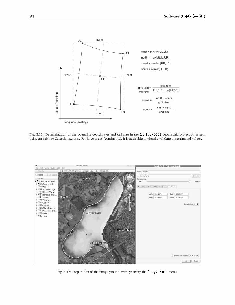
84 Software (R+GIS+GE)
Fig. 3.11: Determination of the bounding coordinates and cell size in the LatLonWGS84 geographic projection systemusing an existing Cartesian system. For large areas (continents), it is advisable to visually validate the estimated values.
Fig. 3.12: Preparation of the image ground overlays using the Google Earth menu.

3.3 Geographical visualization: Google Earth (GE) 85
bounding coordinates and location of the image file (Fig. 3.12). Because the image is located on some server, it 1
can also be automatically refreshed and/or linked to a Web Mapping Service (WMS). For a more sophisticated 2
use of Google interfaces see for example the interactive KML sampler56, that will give you some good ideas 3
about what is possible in Google Earth. Another interactive KML creator that plots various (geographical) CIA 4
World Factbook, World Resources Institute EarthTrends and UN Data is the KML FactBook57. 5
Another possibility to export the gridded maps to R (without resampling grids) is to use the vector structure 6
of the grid, i.e. to export each grid node as a small squared polygon58. First, we can convert the grids to 7
polygons using the maptools package and reproject them to geographic coordinates (Bivand et al., 2008): 8
# generate predictions e.g.:> zinc.rk <- krige(log1p(zinc) ∼ dist+ahn, data=meuse, newdata=meuse.grid,+ model=vgm(psill=0.151, "Exp", range=374, nugget=0.055))> meuse.grid$zinc.rk <- expm1(zinc.rk$var1.pred)# convert grids to pixels (mask missing areas):> meuse.pix <- as(meuse.grid["zinc.rk"], "SpatialPixelsDataFrame")# convert grids to polygons:> grd.poly <- as.SpatialPolygons.SpatialPixels(meuse.pix)# The function is not suitable for high-resolution grids!!> proj4string(grd.poly) <- CRS("+init=epsg:28992")> grd.poly.ll <- spTransform(grd.poly, CRS("+proj=longlat +datum=WGS84"))> grd.spoly.ll <- SpatialPolygonsDataFrame(grd.poly.ll,+ data.frame(meuse.pix$zinc.rk), match.ID=FALSE)
Next, we need to estimate the Google codes for colors for each polygon. The easiest way to achieve this is 9
to generate an RGB image in R, then reformat the values following the KML tutorial: 10
> tiff(file="zinc_rk.tif", width=meuse.grid@[email protected][1],+ height=meuse.grid@[email protected][2], bg="transparent")> par(mar=c(0,0,0,0), xaxs="i", yaxs="i", xaxt="n", yaxt="n")> image(as.image.SpatialGridDataFrame(meuse.grid["zinc.rk"]), col=bpy.colors())> dev.off()# read RGB layer back into R:> myTile <- readGDAL("zinc_rk.tif", silent=TRUE)> i.colors <- myTile@data[[email protected],]> i.colors[1:3,]
band1 band2 band369 72 0 255146 94 0 255147 51 0 255
> i.colors$B <- round(i.colors$band3/255*100, 0)> i.colors$G <- round(i.colors$band2/255*100, 0)> i.colors$R <- round(i.colors$band1/255*100, 0)# generate Google colors:> i.colors$FBGR <- paste("9d", ifelse(i.colors$B<10, paste("0", i.colors$B, sep=""),+ ifelse(i.colors$B==100, "ff", i.colors$B)),+ ifelse(i.colors$G<10, paste("0", i.colors$G, sep=""),+ ifelse(i.colors$G==100, "ff", i.colors$G)),+ ifelse(i.colors$R<10, paste("0", i.colors$R, sep=""),+ ifelse(i.colors$R==100, "ff", i.colors$R)), sep="")> i.colors$FBGR[1:3]
[1] "9dff0028" "9dff0037" "9dff0020"
and we can write Polygons to KML with color attached in R: 11
56http://kml-samples.googlecode.com/svn/trunk/interactive/index.html57http://www.kmlfactbook.org/58This is really recommended only for fairly small grid, e.g. with�106 grid nodes.

86 Software (R+GIS+GE)
> varname <- "zinc_rk" # variable name> filename <- file(paste(varname, "_poly.kml", sep=""), "w")> write("<?xml version=\"1.0\" encoding=\"UTF-8\"?>", filename)> write("<kml xmlns=\"http://earth.google.com/kml/2.2\">", filename, append = TRUE)> write("<Document>", filename, append = TRUE)> write(paste("<name>", varname, "</name>", sep=" "), filename, append = TRUE)> write("<open>1</open>", filename, append = TRUE)> for (i in 1:length(grd.spoly.ll@data[[1]])) {> write(paste(' <Style id="','poly', i,'">',sep=""), filename, append = TRUE)> write(" <LineStyle>", filename, append = TRUE)> write(" <width>0.5</width>", filename, append = TRUE)> write(" </LineStyle>", filename, append = TRUE)> write(" <PolyStyle>", filename, append = TRUE)> write(paste(' <color>', i.colors$FBGR[i], '</color>', sep=""),+ filename, append = TRUE)> write(" </PolyStyle>", filename, append = TRUE)> write(" </Style>", filename, append = TRUE)> }> write("<Folder>", filename, append = TRUE)> write(paste("<name>Poly ID", varname,"</name>"), filename, append = TRUE)> for (i in 1:length(grd.spoly.ll@data[[1]])) {> write(" <Placemark>", filename, append = TRUE)> write(paste(" <name>", grd.spoly.ll@polygons[[i]]@ID, "</name>", sep=""),+ filename, append = TRUE)> write(" <visibility>1</visibility>", filename, append = TRUE)> write(paste(" <styleUrl>#poly", i, "</styleUrl>", sep=""), filename, append = TRUE)> write(" <Polygon>", filename, append = TRUE)> write(" <tessellate>1</tessellate>", filename, append = TRUE)> write(" <altitudeMode>extruded</altitudeMode>", filename, append = TRUE)> write(" <outerBoundaryIs>", filename, append = TRUE)> write(" <LinearRing>", filename, append = TRUE)> write(" <coordinates>", filename, append = TRUE)> write(paste(" ", grd.spoly.ll@polygons[[i]]@Polygons[[1]]@coords[1,1], ",",+ grd.spoly.ll@polygons[[i]]@Polygons[[1]]@coords[1,2], ",1", sep=""),+ filename, append = TRUE)> write(paste(" ", grd.spoly.ll@polygons[[i]]@Polygons[[1]]@coords[2,1], ",",+ grd.spoly.ll@polygons[[i]]@Polygons[[1]]@coords[2,2], ",1", sep=""),+ filename, append = TRUE)> write(paste(" ", grd.spoly.ll@polygons[[i]]@Polygons[[1]]@coords[3,1], ",",+ grd.spoly.ll@polygons[[i]]@Polygons[[1]]@coords[3,2], ",1", sep=""), ",",+ filename, append = TRUE)> write(paste(" ", grd.spoly.ll@polygons[[i]]@Polygons[[1]]@coords[4,1], ",",+ grd.spoly.ll@polygons[[i]]@Polygons[[1]]@coords[4,2], ",1", sep=""),+ filename, append = TRUE)> write(paste(" ", grd.spoly.ll@polygons[[i]]@Polygons[[1]]@coords[5,1], ",",+ grd.spoly.ll@polygons[[i]]@Polygons[[1]]@coords[5,2], ",1", sep=""),+ filename, append = TRUE)> write(" </coordinates>", filename, append = TRUE)> write(" </LinearRing>", filename, append = TRUE)> write(" </outerBoundaryIs>", filename, append = TRUE)> write(" </Polygon>", filename, append = TRUE)> write(" </Placemark>", filename, append = TRUE)> }> write("</Folder>", filename, append = TRUE)> write("</Document>", filename, append = TRUE)> write("</kml>", filename, append = TRUE)> close(filename)
In similar fashion, time-series of maps (range of maps covering the same geographic domain, but referring1
to a different time period) can be exported and explored in Google Earth using time-slider. Note also that2
a list of remotely sensed image bands or maps produced by geostatistical simulations can be exported as a3

3.3 Geographical visualization: Google Earth (GE) 87
time-series, and then visualized as animation. The maptools package is not able to generate GE KMLs using 1
space-time data59, but we can instead write directly a KML file from R. An example is further shown in 2
section 11.5.3. 3
Users of MatLab can explore possibilities for exporting the results of geostatistical analysis to Google Earth 4
by using the Google Earth Toolbox60. This toolbox serves not only to export maps (vectors, ground overlays), 5
but also as a friendly tool to export the associated legends, generate 3D surfaces, contours from isometric 6
maps, wind barbs and 3D vector objects. For example, a gridded map produced using some spatial prediction 7
technique can be converted to a KML format using e.g.: 8
MATLAB: examplemap = ge_groundoverlay(N,E,S,W,... 'imageURL','mapimage.png');MATLAB: ge_output('examplemap.kml',kmlStr);
where N,E,S,W are the bounding coordinates that can be determined automatically or set by the user. 9
3.3.3 Reading KML files to R 10
In principle, everything we export from R to KML we can also read back into R. GDAL has an OGR KML driver 11
that should work for vector data also on Windows OS with the standard rgdal binary. The GDAL website6112
indicates that KML reading is only available if GDAL/OGR is built with the Expat XML Parser, otherwise 13
only KML writing will be supported. Supported OGR geometry types are: Point, Linestring, Polygon, 14
MultiPoint, MultiLineString, MultiPolygon and MultiGeometry. Unfortunately, reading of more complex 15
KML files is still a cumbersome. Reading of KML files can not easily be automated because the code often 16
requires editing, for the simple reason that KML does not (yet) have standard spatial data formats. 17
The most recent version of the package maptools contains methods (e.g. getKMLcoordinates) to read 18
KML files to R and coerce them to the sp formats. KML could carry a lot of non-spatial information, or 19
spatial information that is not supported by most GIS (e.g. viewing angle, transparency, description tags, style 20
definition etc.). In addition, you could have more maps within the same KML file, which makes it difficult to 21
automate import of KML files to a GIS. 22
To read the point map meuse_lead.kml we exported previously using the writeOGR method, we can always 23
use the XML62 package: 24
> library(XML)> meuse_lead.kml <- xmlTreeParse("meuse_lead.kml")> lengthp <- length(meuse_lead.kml$doc[[1]][[1]][[1]])-1> lead_sp <- data.frame(Longitude=rep(0,lengthp), Latitude=rep(0,lengthp),+ Var=rep(0,lengthp))> for(j in 1:lengthp) {> LatLon <- unclass(meuse_lead.kml$doc[[1]][[1]][[1]][j+1][[1]][2][[1]][[1]][[1]])$value> Var <- unclass(meuse_lead.kml$doc[[1]][[1]][[1]][j+1][[1]][1][[1]][[1]])$value> lead_sp$Longitude[[j]] <- as.numeric(matrix(unlist(strsplit(LatLon,+ split=",")), ncol=2)[1])> lead_sp$Latitude[[j]] <- as.numeric(matrix(unlist(strsplit(LatLon,+ split=",")), ncol=2)[2])> lead_sp$Var[[j]] <- as.numeric(matrix(unlist(strsplit(strsplit(Var,+ split="<i>")[[1]][2], split="</i>")), ncol=2)[1])> }> coordinates(lead_sp) <- ∼ Longitude+Latitude> proj4string(lead_sp) <- CRS("+proj=longlat +ellps=WGS84")> bubble(lead_sp, "Var")
Note that it will take time until you actually locate where in the KML file the coordinates of points and 25
attribute values are located (note long lines of sub-lists). After that it is relatively easy to automate creation 26
of a SpatialPointsDataFrame. This code could be shorten by using the xmlGetAttr(), xmlChildren() and 27
xmlValue() methods. You might also consider using the KML2SHP63 converter (ArcView script) to read KML 28
files (points, lines, polygons) and generate shapefiles directly from KML files. 29
59The new stpp package (see R-forge) is expected to bridge this gap.60http://www.mathworks.com/matlabcentral/fileexchange/1295461http://www.gdal.org/ogr/drv_kml.html62http://cran.r-project.org/web/packages/XML/63http://arcscripts.esri.com/details.asp?dbid=14988

88 Software (R+GIS+GE)
3.4 Summary points1
3.4.1 Strengths and limitations of geostatistical software2
Both open source and proprietary software packages have strong and weak points. A comparison of different3
aspects of geostatistical packages listed at the AI-Geostats website64 and several well-known GIS packages4
can be seen in Table 3.1. Although universal kriging (using coordinates) is available in most geostatistical5
packages, kriging with external drift with multiple auxiliary maps can be run in only a limited number of6
packages. From all software listed in Table 3.1, only Isatis, SAGA, and gstat/geoR (as stand-alone application7
or integrated into R) offer the possibility to interpolate a variable using (multiple) auxiliary maps (Hengl8
et al., 2007a). Note that the comparison of packages is not trivial because many proprietary packages rely9
on plugins/toolboxes that are either distributed separately or are valid for certain software versions only. For10
example, ArcGIS has excellent capabilities for writing and reading KML files, but the user needs to obtain the11
Arc2Earth package, which is sold separately.12
Hengl et al. (2007a) tested regression-kriging in variety of packages to discover that RK in Isatis is limited13
to use of a single (three in script mode) auxiliary maps (Bleines et al., 2004). In gstat, both RK predictions14
and simulations (predictors as base maps) at both point and block support can be run by defining short scripts,15
which can help automatize interpolation of large amounts of data. However, gstat implements the algorithm16
with extended matrix (KED), which means that both the values of predictors and of target variable are used17
to estimate the values at each new location, which for large data sets can be time-consuming or can lead18
to computational problems (Leopold et al., 2005). geoR stands out as a package with the most sophisticated19
approaches to model estimation, but it is not really operational for use with large data sets. It was not designed20
to work with common spatial classes and data formats and some manual work is needed to get the maps out21
(see further section 5.5.3).22
Fig. 3.13: Trends in the web-traffic for esri.com, r-project.org andosgeo.org (following the trends.google.com statistics).
Setting RK in gstat or SAGA to a smaller23
window search can lead to termination of the24
program due to singular matrix problems65. In25
fact, local RK with a global variogram model is26
not entirely valid because the regression model27
will differ locally, hence the algorithm should28
also estimate the variogram model for residuals29
for each local neighborhood (as mentioned pre-30
viously in §2.2). The singular matrix problem31
will happen especially when indicator variables32
are used as predictors or if the two predictor33
maps are highly correlated. Another issue is the34
computational effort. Interpolation of � 10335
points over 1M of pixels can last up to several36
hours on a standard PC. To run simulations in37
R+gstat with the same settings will take even38
more time. This proves that, although the KED39
procedure is mathematically elegant, it might40
be more effective for real-life applications to fit41
the trend and residuals separately (the regression-kriging approach). A limitation of gstat.exe is that it is42
a stand-alone application and the algorithms cannot be adjusted easily. Unlike the gstat package in R that43
can be extended and then uploaded by anybody. A limitation of R, however, is that it can reach memory use44
problems if larger rasters or larger quantities of rasters are loaded into R. Visualization and visual exploration45
of large maps in R is also not recommended.46
So in summary, if you wish to fit your data in a statistically optimal way and with no limitations on the47
number of predictors and statistical operations — R and packages gstat and geoR are the most professional48
choice. If you do not feel confident about using software environment without an interface, then you could try49
running global Universal kriging in SAGA. However, SAGA does not provide professional variogram modeling50
capabilities, so a combination R+GIS+GE is probably the best idea. In fact, the computation is a bit faster in51
SAGA than in R and there are no memory limit problems (see further section 5.5.2). However, in SAGA you52
64http://ai-geostats.org65You can prevent gstat from breaking predictions by setting the krige option set=list(cn_max=1e10, debug=0).

3.4 Summary points 89
Table 3.1: Comparison of spatio-temporal data analysis capabilities of some popular statistical and GIS packages (versionsin year 2009): Æ— full capability, ?— possible but with many limitations, −— not possible in this package. Commercialprice category: I — > 1000 EUR; II — 500-1000 EUR; III — < 500 EUR; IV — open source or freeware. Main application:A — statistical analysis and data mining; B — interpolation of point data; C — processing / preparation of input maps; E— visualization and visual exploration. After Hengl et al. (2007a).
Aspect S-PLUS
R+gstat
R+geoR
MatLab
SURFER
ISATIS
GEOEas
GSLIB
GRASS
PCRaster
ILWIS
IDRISI
ArcGIS
SAGA
Commercial pricecategory
II IV IV I III I IV IV IV III IV II I IV
Main application A, B A, B A, B A, E B, E B B B B, C C B, C B, C B, E B, C
User-friendlyenvironment tonon-expert
Æ − − Æ Æ Æ − − ? − Æ Æ Æ Æ
Quality of support anddescription of algorithms
? Æ Æ Æ Æ Æ Æ Æ ? ? Æ Æ ? ?
Standard GIS capabilities − ? − ? ? − − − Æ ? Æ Æ Æ Æ
GDAL support − Æ ? ? − ? − − Æ ? ? Æ Æ ?
Standard descriptivestatistical analysis
Æ Æ Æ Æ − Æ ? ? ? − Æ Æ Æ ?
Image processing tools(orthorectification,filtering, land surfaceanalysis)
− − − ? − − − − Æ − Æ Æ ? Æ
Comprehensiveregression analysis(regression trees, GLM)
Æ Æ Æ Æ − ? − − − − − ? − −
Interactive (automated)variogram modeling
− ? Æ − − Æ − ? − − − Æ Æ −
Regression-kriging withauxiliary maps
− Æ ? − − ? − − Æ ? ? Æ − Æ
Dynamic modeling(simulations, spatialiterations, propagation,animations)
− ? ? ? − − − − ? Æ ? ? ? ?
Processing of large datasets
Æ ? − ? ? Æ − − Æ ? ? Æ Æ Æ
Export of maps to GoogleEarth (KML)
− Æ ? Æ − − − − ? − − ? Æ −

90 Software (R+GIS+GE)
will not be able to objectively estimate the variogram of residuals or GLS model for the deterministic part of1
variation.2
The R+SAGA/GRASS+GE combo of applications allows full GIS + statistics integration and can support3
practically 80% of processing/visualization capabilities available in proprietary packages such as ArcInfo/Map4
or Idrisi. The advantage of combining R with open source GIS is that you will be able to process and visualize5
even large data sets, because R is not really suited for processing large data volumes, and it was never meant6
to be used for visual exploration or editing of spatial data. On the other hand, packages such as ILWIS and7
SAGA allow you to input, edit and visually explore geographical data, before and after the actual statistical8
analysis. Note also that ILWIS, SAGA and GRASS extend the image processing functionality (especially image9
filtering, resampling, geomorphometric analysis and similar) of R that is, at the moment, limited to only few10
experimental packages (e.g. biOps, rimage; raster66). An alternative for GIS+R integration is QGIS67, which11
has among its main characteristics a python console, and a very elaborate way of adding Python plugins, which12
is already in use used for an efficient R plugin (manageR).13
In principle, we will only use open source software to run the exercises in this book, and there are several14
good reasons. Since the 1980’s, the GIS research community has been primarily influenced by the (proprietary)15
software licence practices that limited sharing of ideas and user-controlled development of new functionality16
(Steiniger and Bocher, 2009). With the initiation of the Open Source Geospatial Foundation (OSGeo), a17
new era began: the development and use of open source GIS has experienced a boom over the last few years;18
the enthusiasm to share code, experiences, and to collaborate on projects is growing (Bivand, 2006).19
Steiniger and Bocher (2009) recognize four indicators of this trend: (1) increasing number of projects run20
using the open source GIS, (2) increasing financial support by government agencies, (3) increasing download21
rates, and (4) increasing number of use-cases. By comparing the web-traffic for proprietary and open source22
GIS (Fig. 3.13) one can notice that OSGeo has indeed an increasing role in the world market of GIS. Young23
and senior researchers are slowly considering switching from using proprietary software such as ESRI’s ArcGIS24
and/or Mathworks’ MatLab to R+SAGA, but experience (Windows vs Linux) teaches us that it would be25
over-optimistic to expect that this shift will go fast and without resistance.26
3.4.2 Getting addicted to R27
From the previously-discussed software tools, one software needs to be especially emphasized, and that is R28
(R Development Core Team, 2009). Many R users believe that there is not much in statistics that R cannot29
do68 (Zuur et al., 2009). Certainly, the number of packages is increasing everyday, and so is the community.30
There are at least five good (objective) reasons why you should get deeper into R (Rossiter, 2009):31
It is of high quality — It is a non-proprietary product of international collaboration between top statisticians.32
It helps you think critically — It stimulates critical thinking about problem-solving rather than a push the33
button mentality.34
It is an open source software — Source code is published, so you can see the exact algorithms being used;35
expert statisticians can make sure the code is correct.36
It allows automation — Repetitive procedures can easily be automated by user-written scripts or functions.37
It helps you document your work — By scripting in R, anybody is able to reproduce your work (processing38
metadata). You can record steps taken using history mechanism even without scripting, e.g. by using39
the savehistory() command.40
It can handle and generate maps — R now also provides rich facilities for interpolation and statistical anal-41
ysis of spatial data, including export to GIS packages and Google Earth.42
The main problem with R is that each step must be run via a command line, which means that the analyst43
must really be an R expert. Although one can criticize R for a lack of an user-friendly interface, in fact,44
most power users in statistics never use a GUI. GUI’s are fine for baby-steps and getting started, but not for45
66http://r-forge.r-project.org/projects/raster/ — raster is possibly the most active R spatial project at the moment.67http://qgis.org/68This is probably somewhat biased statement. For example, R is not (yet) operational for processing of large images (filter analysis,
map iterations etc.), and many other standard geographical analysis steps are lacking.

3.4 Summary points 91
production work. The whole point is that one can develop a script or program that, once it is right, can be 1
re-run and will produce exactly the same results each time (excluding simulations of course). 2
Here are some useful tips on how to get addicted to R. First, you should note that you can edit the R scripts 3
in user-friendly script editors such as Tinn-R69 or use the package R commander (Rcmdr70), which has an 4
user-friendly graphical interface. Second, you should take small steps before you get into really sophisticated 5
script development. Start with some simple examples and then try to do the same exercises with your own 6
data. The best way to learn R is to look at existing scripts. For example, a French colleague, Romain François, 7
maintains a gallery of R graphics71 that is dedicated to the noble goal of getting you addicted to R. A similar- 8
purpose website is the R Graphical Manual72. Robert I. Kabacoff maintains a website called Quick-R73 that 9
gives an overview of R philosophy and functionality. John Verzani maintains a website with simple examples 10
in R that will get you going74. If you love cookbooks, R has those too75. In fact, you might make the following 11
package the first you try. Type the following command into R to (1) download a tutorial package; (2) load the 12
package in R; and (3) tell R to open a webpage with more information about the tutorial (Verzani, 2004): 13
> install.packages("UsingR")> library(UsingR)> UsingR("exercises")
Third, if your R script does not work, do not despair, try to obtain some specialized literature. Reading 14
specialized literature from the experts is possibly the best way to learn script writing in R. Start with Zuur et al. 15
(2009), then continue with classics such as Chambers and Hastie (1992), Venables and Ripley (2002) and/or 16
Murrell (2006). Other excellent and freely available introductions to R are Kuhnert and Venables (2005), 17
Burns (2009) and Rossiter (2009). If you are interested in running spatial analysis or geostatistics in R, then 18
books by Bivand et al. (2008), Baddeley (2008) Reimann et al. (2008), and/or Diggle and Ribeiro Jr (2007) 19
are a must. 20
Getting help 21
Because the R community is large, chances are good that the problems you encounter have already been solved 22
or at least discussed, i.e. it is already there. The issue is how to find this information. There are several sources 23
where you should look: 24
(1.) the help files locally installed on your machine; 25
(2.) mailing/discussion lists; 26
(3.) various website and tutorials, and 27
(4.) books distributed by commercial publishers; 28
You should really start searching in this order — from your machine to a bookstore — although it is always 29
a good idea to cross-check all possible sources and compare alternatives. Please also bear in mind that (a) 30
not everything that you grab from www is correct and up-to-date; and (b) it is also possible that you have an 31
original problem that nobody else has experienced. 32
Imagine that you would like to find out which packages on your machine can run interpolation by kriging. 33
You can quickly find out this by running the method help.search, which will give something like this: 34
> help.search("kriging")
Help files with alias or concept or title matching 'kriging' using fuzzy matching:
image.kriging(geoR) Image or Perspective Plot with Kriging Resultskrige.bayes(geoR) Bayesian Analysis for Gaussian Geostatistical Models
69http://www.sciviews.org/Tinn-R/70http://socserv.mcmaster.ca/jfox/Misc/Rcmdr/71http://addictedtor.free.fr72http://bm2.genes.nig.ac.jp/RGM2/73http://www.statmethods.net74http://www.math.csi.cuny.edu/Statistics/R/simpleR/75http://www.r-cookbook.com

92 Software (R+GIS+GE)
krige.conv(geoR) Spatial Prediction -- Conventional Krigingkrweights(geoR) Computes kriging weightsksline(geoR) Spatial Prediction -- Conventional Kriginglegend.krige(geoR) Add a legend to a image with kriging resultswo(geoR) Kriging example data from Webster and Oliverxvalid(geoR) Cross-validation by krigingkrige(gstat) Simple, Ordinary or Universal, global or local,
Point or Block Kriging, or simulation.krige.cv(gstat) (co)kriging cross validation, n-fold or leave-one-outossfim(gstat) Kriging standard errors as function of grid spacing
and block sizekrige(sgeostat) Krigingprmat(spatial) Evaluate Kriging Surface over a Gridsemat(spatial) Evaluate Kriging Standard Error of Prediction over a Grid
Type 'help(FOO, package = PKG)' to inspect entry 'FOO(PKG) TITLE'.
This shows that kriging (and its variants) is implemented in (at least) four packages. We can now display1
the help for the method "krige" that is available in the package gstat:2
> help(krige, package=gstat)
The archives of the mailing lists are available via the servers in Zürich. They are fairly extensive and the3
best way to find something useful is to search them. The fastest way to search all R mailing lists is to use the4
RSiteSearch method. For example, imagine that you are trying to run kriging and then the console gives you5
the following error message e.g.:6
"Error : dimensions do not match: locations XXXX and data YYYY"
Based on the error message we can list at least 3–5 keywords that will help us search the mailing list, e.g.:7
> RSiteSearch("krige {dimensions do not match}")
This will give over 15 messages76 with a thread matching exactly your error message. This means that8
other people also had this problem, so now you only need to locate the right solution. You should sort the9
messages by date and then start from the most recent message. The answer to your problem will be in one of10
the replies submitted by the mailing list subscribers. You can quickly check if this is a solution that you need11
by making a small script and then testing it.12
Of course, you can at any time Google the key words of interest. However, you might instead consider13
using the Rseek.org77 search engine maintained by Sasha Goodman. The advantage of using Rseek over e.g.14
general Google is that it focuses only on R publications, mailing lists, vignettes, tutorials etc. The result of the15
search is sorted in categories, which makes it easier to locate the right source.16
If you are eventually not able to find a solution yourself, you can try sending the description of your17
problem to a mailing list, i.e. asking the R gurus. Note that there are MANY R mailing lists78, so you first have18
to be sure to find the right one. Sending a right message to a wrong mailing list will still leave you without an19
answer. Also have in mind that everything you send to a mailing list is public/archived, so better cross-check20
your message before you send it. When asking for a help from a mailing list, use the existing pre-installed data21
sets to describe your problem79.22
Do’s:23
If you have not done so already, read the R posting guide80!24
Use the existing pre-installed data sets (come together with a certain package) to describe your25
problem. You can list all available data sets on your machine by typing data(). This way you do not26
have to attach your original data or waste time on trying to explain your case study.27
76Unfortunately, RSiteSearch() no longer searches R-sig-geo — the full archive of messages is now on Nabble.77http://rseek.org78There are several specific Special Interest Group mailing lists; see http://www.r-project.org/mail.html.79Then you only need to communicate the problem and not the specifics of a data set; there is also no need to share your data.80http://www.r-project.org/posting-guide.html

3.4 Summary points 93
If your problem is completely specific to your data set, then upload it an put it on some web-directory 1
so that somebody can access it and see what really goes on. 2
Link your problem to some previously described problems; put it in some actual context (to really 3
understand what I mean here, you should consider attending the Use R conferences). 4
Acknowledge the work (time spent) other people do to help you. 5
You can submit not only the problems you discover but also the information that you think is interest- 6
ing for the community. 7
Don’ts: 8
Do not send poorly formulated questions. Make sure you give technical description of your data, 9
purpose of your analysis, even the details about your operating system, RAM etc. Try to put yourself in 10
a position of a person that is interested to help — try to provide all needed information as if the person 11
who is ready to help you would feel like sitting at your computer. 12
Do not send too much. One message, one question (or better to say “one message, one problem”). 13
Nobody reading R mailing lists has time to read long articles with multiple discussion points. Your 14
problem should fit half the page; if somebody gets more interested, you can continue the discussion also 15
off the list. 16
R comes with ABSOLUTELY NO WARRANTY. If you loose data or get strange results, you are welcome 17
to improve the code yourself (or consider obtaining some commercial software). Complaining to a 18
mailing list about what frustrates you about R makes no sense, because nobody is obliged to take 19
any responsibility. 20
R is a community project (it is based on the solidarity between the users). Think what you can do for 21
the community and not what the community can do for you. 22
Probably the worst thing that can happen to your question is that you do not get any reply (and this does 23
not necessarily mean that nobody wants to help you or that nobody know the solution)! There are several 24
possible reasons why this happened: 25
You have asked too much! Some people post questions that could take weeks to investigate (maybe this 26
justifies a project proposal?). Instead, you should always limit yourself to 1-2 concrete issues. Broader 27
discussions about various more general topics and statistical theory are sometimes also welcome, but 28
they should be connected with specific packages. 29
You did not introduce your question/topic properly. If your question is very specific to your field and 30
the subscribers cannot really understand what you are doing, you need to think of ways to introduce 31
your field and describe the specific context. The only way to learn the language used by the R mailing 32
lists is to browse the existing mails (archives). 33
You are requesting that somebody does a work for you that you could do yourself! R and its 34
packages are all open source, which allows YOU to double check the underlying algorithms and extend 35
them where necessary. If you want other people to do programming for you, then you are at the wrong 36
place (some commercial software companies do accept wish-lists and similar types of requests, but that’s 37
what they are paid for anyway). 38
Your question has been answered already few times and it is quite annoying that you did not do 39
your homework to check this. 40
Remember: everything you send to mailing lists reach large audiences (for example, R-sig-geo has +1000 41
subscribers), and it is archived on-line, so you should be more careful about what you post. If you develop a 42
bad reputation of being ignorant and/or too sloppy, then people might start ignoring your questions even if 43
they eventually start getting the right shape. 44

94 Software (R+GIS+GE)
Tips for successful scripting in R1
R is a command line based environment, but users do really write things directly to a command line. It is2
more common to first write using text editors (e.g. Tinn-R, JGR) and then “send lines” of code to R command3
line. When generating an R script, there are few useful tips that you might consider following (especially if4
you plan to share this script with a wider community):5
Document your code to explain what you are doing. Comments in R can be inserted after the "#" sign;6
You can never put too many comments in your code!7
Add some meta-information about the script at the beginning of your script — its authors, last8
update, purpose, inputs and outputs, reference where somebody can find more info (R scripts usually9
come as supplementary materials for project reports or articles) and difficulties one might experience.10
In many situations it is also advisable to mention the package version used to generate outputs. Because11
R is dynamic and many re-designs happen, some old scripts might become incompatible with the new12
packages.13
Once you tested your script and saw that it works, tidy-up the code — remove unnecessary lines,14
improve the code where needed, and test it using extreme cases (Burns (2009) provides some useful15
tips on how to improve scripting). In R, many equivalent operations can be run via different paths.16
In fact, the same techniques are commonly implemented in multiple packages. On the other hand,17
not all methods are equally efficient (speed, robustness), i.e. equally elegant, so that it is often worth18
investigating what might be the most elegant way to run some analysis. A good practice is to always19
write a number of smaller functions and then a function that does everything using the smaller functions.20
Note also that the variable names and list of input maps can be save and dealt with as with lists (see e.g.21
page166).22
Place the data sets on-line (this way you only need to distribute the script) and then call the data by23
using the download.file method in R;24
All these things will make a life easier for your colleagues, but also to yourself if you decide to come back25
to your own script in few years (or few months). Another thing you might consider is to directly write the code26
and comments in Tinn-R using the Sweave81 package. Note that you can still run this script from Tinn-R, you27
only need to specify where the R code begins (<<>>=) and ends (@). This way, you do not only distribute the28
code, but also all explanation, formulae etc. Building metadata for both the data sets and scripts you produce29
is becoming increasingly important.30
Memory limit problems31
Another important aspect to consider is R’s ability to handle large data sets. Currently, many pharmaceutical32
organizations and financial institutions use R as their primary analytical engine. They crunch huge amounts33
of data, so it works on very large data sets. However loading, displaying and processing large geographic34
data sets like big raster maps (�1M pixels) can be problematic with R. Windows 32–bit OS can allocate a35
maximum of 2 GB of memory to an application82. Even if your computer has >2 GB of RAM, you will receive36
an error message like:37
Error: cannot allocate vector of size 12.6 Mb
which might suggest to you that R has problems with surprisingly small data sets. This message actually means38
R has already allocated all of the 2 GB of memory available to it. Check the system’s memory allocation by39
typing:40
> gc()
and you will find R is already occupying a lot of RAM. The key issue is that R stores data in a temporary41
buffer, which can result in problems with memory availability. However, the benefit of this strategy is it allows42
maximum flexibility in data structures.. For Burns (2009) there are only two solutions to the problem: (1)43
Improve your code; (2) Get a bigger computer!44
To increase your computing capacities, you can also consider doing one of the following:45
81http://www.stat.uni-muenchen.de/~leisch/Sweave/82Read more at: http://www.microsoft.com/whdc/system/platform/server/PAE/PAEmem.mspx

3.4 Summary points 95
Fig. 3.14: Windows task manager showing the CPU and memory usage. Once the computing in R comes close to 2 GB ofphysical memory, Windows will not allow R to use any more memory. The solution to this problem is to use a PC with an64–bit OS.
Reduce the grid resolution of your maps. If you reduce the grid cell size by half, the memory usage will 1
be four times smaller. 2
Consider splitting your data set into tiles. Load data tile by tile, write the results to physical memory or 3
external database, remove temporary files, repeat the analysis until all tiles are finished. This is the so 4
called “database” solution to memory handling (Burns, 2009). 5
Obtain a new machine. Install a 64–bit OS with >10GB of RAM. A 64–bit OS will allow you to use more 6
application memory. 7
Consider obtaining a personal supercomputer83 with a completely customizable OS. Supercomputer is 8
about 200 times faster than your PC, mainly because it facilitates multicore operations. The price of a 9
standard personal supercomputer is about 5–10 times that of a standard PC. 10
During the processing, you might try releasing some free memory by continuously using the gc() com- 11
mand. This will remove some temporary files and hence increase some free memory. If you are Windows OS 12
user, you should closely monitor your Windows Task manager (Fig. 3.14), and then, when needed, use garbage 13
collector (gc()) and/or remove (rm()) commands to increase free space. Another alternative approach is to 14
combine R with other (preferably open-source) GIS packages, i.e. to run all excessive processing externally 15
from R. It is also possible that you could run extensive calculations even with your limited PC. This is because 16
processing is increasingly distributed. For example, colleagues from the Centre for e-Science in Lancaster 17
have been recently developing an R package called MultiR84 that should be able to significantly speed up R 18
calculations by employing grid computing facilities (Grose et al., 2006). 19
83See e.g. http://www.nvidia.com/object/personal_supercomputing.html84http://cran.r-project.org/web/views/HighPerformanceComputing.html

96 Software (R+GIS+GE)
3.4.3 Further software developments1
There are still many geostatistical operations that we are aware of, but have not been implemented and are2
not available to broader public (§2.10.3). What programmers might consider for future is the refinement of3
(local) regression-kriging in a moving window. This will allow users to visualize variation in regression (maps4
of R-square and regression coefficients) and variogram models (maps of variogram parameters). Note that5
the regression-kriging with moving window would need to be fully automated, which might not be an easy6
task considering the computational complexity. Also, unlike OK with a moving window (Walter et al., 2001),7
regression-kriging has much higher requirements considering the minimum number of observations (at least8
10 per predictor, at least 50 to model variogram). In general, our impression is that many of the procedures9
(regression and variogram modeling) in regression-kriging can be automated and amount of data modeling10
definitions expanded (local or global modeling, transformations, selection of predictors, type of GLMs etc.),11
as long as the point data set is large and of high quality. Ideally, users should be able to easily test various12
combinations of input parameters and then (in real-time) select the one that produces the most satisfactory13
predictions.14
Open-source packages open the door to analyzes of unlimited sophistication. However, they were not15
designed with a graphical user interfaces (GUI’s), or wizards typical for proprietary GIS packages. Because of16
this, they are not easily used by non-experts. There is thus opportunity both for proprietary GIS to incorporate17
regression-kriging ideas and for open-source software to become more user-friendly.18
3.4.4 Towards a system for automated mapping19
Geostatistics provides a set of mathematical tools that have been used now over 50 years to generate maps20
from point observations and to model the associated uncertainty. It has proven to be an effective tool for a large21
number of applications ranging from mining and soil and vegetation mapping to environmental monitoring22
and climatic modeling. Several years ago, geostatistical analysis was considered to be impossible without the23
intervention of a spatial analyst, who would manually fit variograms, decide on the support size and elaborate24
on selection of the interpolation technique. Today, the heart of a mapping project can be the computer program25
that implements proven and widely accepted (geo)statistical prediction methods. This leads to a principle of26
automated mapping where the analyst focuses his work only on preparing the inputs and supervising the27
data processing85. This way, the time and resources required to go from field data to the final GIS product28
(geoinformation) are used more efficiently.29
Automated mapping is still utopia for many mapping agencies. At the moment, environmental monitoring30
groups worldwide tend to run analyzes separately, often with incorrect techniques, frequently without making31
the right conclusions, and almost always without considering data and/or results of adjacent mapping groups.32
On one side, the amount of field and remotely sensed data in the world is rapidly increasing (see section 4);33
on the other side, we are not able to provide reliable information to decision makers in near real-time. It34
is increasingly necessary that we automate the production of maps (and models) that depict environmental35
information. In addition, there is an increasing need to bring international groups together and start “piec-36
ing together a global jigsaw puzzle”86 to enable production of a global harmonized GIS of all environmental37
resources. All this proves that automated mapping is an emerging research field and will receive significant38
attention in geography and Earth sciences in general (Pebesma et al., 2009).39
A group of collaborators, including the author of this book, have begun preliminary work to design, de-40
velop, and test a web-based automated mapping system called auto-map.org. This web-portal should allow41
the users to upload their point data and then: (a) produce the best linear predictions depending of the nature/-42
type of a target variable, (b) interpret the result of analysis through an intelligent report generation system,43
(c) allow interactive exploration of the uncertainty, and (d) suggest collection of additional samples — all at44
click of button. The analysis should be possible via a web-interface and through e.g. Google Earth plugin, so45
that various users can access outputs from various mapping projects. All outputs will be coded using the HTML46
and Google Earth (KML) language. Registered users will be able to update the existing inputs and re-run anal-47
ysis or assess the quality of maps (Fig. 3.15). A protocol to convert and synchronize environmental variables48
coming from various countries/themes will need to be developed in parallel (based on GML/GeoSciML87).49
85See for example outputs of the INTAMAP project; http://www.intamap.org.86Ian Jackson of the British Geological Survey; see also the http://www.onegeology.org project.87http://www.cgi-iugs.org

3.4 Summary points 97
Spatial
inference
system
Load field-data (points,
areas) to AUTO-MAP
Select method: interpolation/
simulations, sampling
optimisation, error assessment
Convert outputs to
KML format (ASP script)
including the machine
readable meta-data
Repository of auxiliary data:
- DEM parameters
- RS images
- thematic maps Select optional parameters:
target area (grid size), targeted
precision, maximum iterations
Share outputs to users’ groups:
(a) registered groups
(b) WMS / Google Earth
(1)
(2)
(3)
(5)
OUTPUTS:
- raster maps (GIS data)
- full analysis report (HTML)
- visualisations (JPG)
Evaluate results and approve
their publication/dissemination(4)
PROCESSING STEPS:
INPUTS:
- field-sampled values
Fig. 3.15: A proposal for the flow of procedures in auto-map.org: a web-based system for automated predictive mappingusing geostatistics. The initial fitting of the models should be completely automated; the user then evaluates the resultsand makes eventual revisions.
There would be many benefits of having a robust, near-realtime automated mapping tool with a friendly 1
web-interface. Here are some important ones: 2
the time spent on data-processing would be seriously reduced; the spatial predictions would be available 3
in near real time; 4
through a browsable GIS, such as Google Earth, various thematic groups can learn how to exchange 5
their data and jointly organize sampling and interpolation; 6
the cost-effectiveness of the mapping would increase: 7
– budget of the new survey projects can be reduced by optimising the sampling designs; 8
– a lower amount of samples is needed to achieve equally good predictions; 9
It is logical to assume that software for automated mapping will need to be intelligent. It will not only be 10
able to detect anomalies, but also to communicate this information to users, autonomously make choices on 11
whether to mask out parts of the data sets, use different weights to fit the models or run comparison for various 12
alternatives. This also means that development of such a system will not be possible without a collaboration 13
between geostatisticians, computer scientists and environmental engineers. 14
Many geostatisticians believe that map production should never be based on a black-box system. The 15
author of this guide agrees with these views. Although data processing automation would be beneficial to all, 16
analysts should at any time have the control to adjust the automated mapping system if needed. To do this, 17
they should have full insight into algorithms used and be able to explore input data sets at any moment. 18
Further reading: 19
Æ Bolstad, P., 2008. GIS Fundamentals, 3rd edition. Atlas books, Minnesota, 620 p. 20
Æ Burns, P. 2009. The R Inferno. Burns statistics, London, 103 p. 21

98 Software (R+GIS+GE)
Æ Conrad, O. 2007. SAGA — program structure and current state of implementation. In: Böhner, J.,1
Raymond, K., Strobl, J., (eds.) SAGA — Analysis and modeling applications, Göttinger Geographische2
abhandlungen, Göttingen, pp. 39-52.3
Æ Rossiter, D.G., 2007. Introduction to the R Project for Statistical Computing for use at ITC. Interna-4
tional Institute for Geo-information Science & Earth Observation (ITC), Enschede, Netherlands, 136 p.5
Æ Venables, W. N. and Ripley, B. D., 2002. Modern applied statistics with S. Statistics and computing.6
Springer, New York, 481 p.7
Æ Zuur, A. F., Ieno, E. N., Meesters, E. H. W. G., 2009. A Beginner’s Guide to R. Springer, Use R series,8
228 p.9
Æ http://www.52north.org — 52° North initiative responsible for the distribution of ILWIS GIS.10
Æ http://www.saga-gis.org — homepage of the SAGA GIS project.11
Æ http://cran.r-project.org/web/views/Spatial.html — CRAN Task View: Analysis of Spa-12
tial Data maintained by Roger Bivand.13
4 1
Auxiliary data sources 2
As mention previously in §2.10, geostatistical techniques increasingly rely on the availability of auxiliary data 3
sources, i.e. maps and images of surface and sub-surface features. This chapter reviews some of the widely 4
known sources of remote sensing and digital cartographic data that are of interest for various geostatistical 5
mapping applications. I will first focus on the freely available global data sets and remotely sensed data, and 6
then give an example of how to download and import to GIS various MODIS products using R scripts. A small 7
repository of global maps at 0.1 arcdegree (10 km) resolution is also available from the authors website1 (see 8
further chapter 7). 9
4.1 Global data sets 10
Global maps of our environment (both remote sensing-based and thematic) are nowadays increasingly attrac- 11
tive for environmental modeling at global and continental scales. A variety of publicly available maps can be 12
obtained at no cost at resolutions up to 1 km or better, so that the issue for mapping teams is not any more 13
whether to use this data, but where to obtain it, how to load it to an existing GIS and where to find necessary 14
metadata. The most well known global data sets (sorted thematically) are: 15
Height/geomorphology data — Global SRTM Digital Elevation Model is possibly the most known global 16
environmental data set (Rabus et al., 2003). The area covered is between 60° North and 58° South. 17
It was recorded by X-Band Radar (NASA and MIL, covering 100% of the total global area) and C- 18
Band Radar (DLR and ASI, covering 40%). The non-public DLR-ASI data is available with a resolution 19
of approximately 30 m (1 arcsec). A complete land surface model ETOPO1 Global Relief Model2 20
(Fig. 4.1; includes bathymetry data) is available at resolution of 1 km and can be obtained from the 21
NOAA’s National Geophysical Data Center (Amante and Eakins, 2008). The 90 m SRTM DEMs can be 22
obtained from the CGIAR3 — Consortium for Spatial Information. An updated 1 km resolution global 23
topography map (SRTM30 PLUS4; used by Google Earth) has been prepared by Becker et al. (2009). 24
From June 2009, ASTER-based Global Digital Elevation Model (GDEM) at resolution of 30 m has been 25
made publicly available. The GDEM was created by stereo-correlating the 1.3 million-scene ASTER 26
archive of optical images, covering almost 98% of Earth’s land surface (Hayakawa et al., 2008). The 27
one-by-one-degree tiles can be downloaded from NASA’s EOS data archive and/or Japan’s Ground Data 28
System5. 29
Administrative data — Administrative data can be used to calculate proximity-based parameters and to ori- 30
ent the users geographically. One such global administrative data database is the Global Administra- 31
1http://spatial-analyst.net/worldmaps/ — this repository is constantly updated.2http://ngdc.noaa.gov3http://srtm.csi.cgiar.org4http://topex.ucsd.edu/WWW_html/srtm30_plus.html5http://data.gdem.aster.ersdac.or.jp
99

100 Auxiliary data sources
tive Areas (GADM6) data set. It comprises borders of countries and lower level subdivisions such as1
provinces and counties (more than 100,000 areas). Another important global data set is the World Vec-2
tor Shoreline data set7 at scale 1:250,000 (Soluri and Woodson, 1990). This can be, for example, used3
to derive the global distance from the sea coast. Eight general purpose thematic layers: boundaries,4
transportation, drainage, population centers, elevation, vegetation, land use and land cover (al at scale5
1:1,000,000) can be obtained via the Global Map Data project8.6
Socio-economic data — The most important global socio-economic data layers are the population density7
maps and attached socio-economic variables. The Socioeconomic Data and Applications Center (SEDAC9)8
distributes the global population density maps at resolution of 1 km for periods from 1990 up to 20159
(projected density).10
Water resources — The most detailed and the most accurate inventory of the global water resources is the11
Global Lakes and Wetlands Database (GLWD10), which comprises lakes, reservoirs, rivers, and differ-12
ent wetland types in the form of a global raster map at 30-arcsec resolution (Lehner and Doll, 2004).13
Shapefiles of the World basins and similar vector data can be best obtained via the Remote Sensing and14
GIS Unit of the International Water Management Institute (IWMI).15
Lights at night images — Images of lights at night have shown to be highly correlated with industrial activity16
and Gross Domestic Product (Doll et al., 2007). A time-series of annual global night light images is17
available via NOAA’s National Geophysical Data Center11. The lights at night map contains the lights18
from cities, towns, and other sites with persistent lighting, including gas flares. The filtered annual19
composites are available from 1992 until 2003.20
Land cover maps — Land cover maps are categorical-type maps, commonly derived using semi-automated21
methods and remotely sensed images as the main input. A Global Land Cover map for the year 200022
(GLC200012) at 1 km resolution is distributed by the Joint Research Centre in Italy (Bartholome at23
al., 2002). A slightly outdated (1998) global map of land cover is the AVHRR Global Land Cover24
Classification13, provided at resolutions of 1 and 8 km (Hansen et al., 2000). More detailed land25
cover maps are distributed nationally. Ellis and Ramankutty (2000) prepared the first global map of the26
anthropogenic biomes (18 classes) showing dense settlements, villages, croplands, rangelands, forested27
lands and wildlands. The International Water Management Institute also produced the Global map of28
Irrigated Areas14 (GMIA; 28 classes) and the Global map of Rainfed Cropped Areas (GMRCA), both at29
10 km resolution, and based on twenty years of AVHRR images, augmented with higher resolution SPOT30
and JERS-1 imagery.31
Climatic maps — Hijmans et al. (2005) produced global maps of bioclimatic parameters (18) derived32
(thin plate smoothing splines) using >15,000 weather stations. The climatic parameters include: mean,33
minimum and maximum temperatures, monthly precipitation and bioclimatic variables15.34
Ecoregions / Biogeographic regions — Ecoregions are terrestrial, freshwater and/or marine areas with char-35
acteristic combinations of soil and landform that characterize that region. Olson et al. (2001) produced36
the Terrestrial Ecoregions16 global data set, which shows some 867 distinct eco-units, including the37
relative richness of terrestrial species by ecoregion. A somewhat more generalized is the FAO’s map of38
Eco-floristic regions17 (e.g. boreal coniferous forest, tropical rainforest, boreal mountain system etc.).39
Soil / Geology maps — USGS produced a detailed Global Soil Regions map18 at resolution of 60 arcsec.40
FAO, IIASA, ISRIC, ISSCAS, JRC have recently produced a 1 km gridded map, merged from various na-41
6http://biogeo.berkeley.edu/gadm/7http://rimmer.ngdc.noaa.gov/mgg/coast/wvs.html8http://www.iscgm.org9http://sedac.ciesin.columbia.edu/gpw/
10http://www.worldwildlife.org/science/data/item1877.html11http://ngdc.noaa.gov/dmsp/global_composites_v2.html12http://www-tem.jrc.it/glc2000/13http://glcf.umiacs.umd.edu/data/landcover/data.shtml14http://www.iwmigiam.org/info/gmia/15The 1 km resolution maps can be obtained via http://worldclim.org.16http://www.worldwildlife.org/science/ecoregions/item1267.html17http://cdiac.ornl.gov/ftp/global_carbon/18http://soils.usda.gov/use/worldsoils/mapindex/order.html

4.1 Global data sets 101
tional soil maps, which is also known as the Harmonized World Soil Database19 (v 1.1). The geological 1
maps are now being integrated via the OneGeology project. USDA Soil Survey Division also distributes 2
a global map of wetlands (includes: upland, lowland, organic, permafrost and salt affected wetlands). 3
International Soil Reference Information Center (ISRIC) maintains a global soil profile database with 4
over 12,000 profiles and over 50 analytical and descriptive parameters (Batjes, 2009). From NOAA’s 5
National Geophysical Data Center one can obtain a point map with all major earth quakes (Significant 6
Earthquake Database20; with cca 5000 quakes). 7
Forest / wildlife resources — There are two important global forest/wildlife data sets: (1) The world map 8
of intact forest landscapes21 (hardly touched by mankind) at a scale 1:1,000,000 (includes four classes 9
of intact forests: 1. intact closed forests; 2. intact open forests, 3. woodlands and savannas, closed 10
forests; and 4. open forests, woodlands and savannas) — maintained by the Greenpeace organization 11
(Potapov, P. et al., 2008), and (2) World Wilderness Areas22 at scale 1:1,000,000 — distributed via the 12
UNEP GEO Data Portal (McCloskey and Spalding, 1989). 13
Biodiversity / human impacts maps — Global maps of biodiversity measures for various groups of taxa (e.g. 14
vascular plants, birds and mammals) can be browsed using the World Atlas of Biodiversity viewer 15
(Groombridge and Jenkins, 2002). Similar type of maps can be browsed via the UNEP’s World Con- 16
servation Monitoring Centre23. Kreft and Jetz (2007) recently produced a global map of plant species 17
diversity (number of plant species) by using field records from 1,032 locations. Partners in the GLO- 18
BIO consortium created a World Map of Human Impacts24 on the Biosphere. This is basically a map 19
showing a current status of the roads, railways and settlement density. The Carbon Dioxide Information 20
Analysis Center provides access to numerous ecological layers and data of interest to global ecologists. 21
One such product is the Global Biomass Carbon Map25 (Carbon density tones of C ha−1), prepared for 22
year 2000 (Ruesch and Gibbs, 2008a). 23
Fig. 4.1: The 1 km resoluton ETOPO1 Global Relief Model (includes bathymetry data). Elevation is probably the mostwidely used global environmental data set — it is available globally at resolutions from 1 km up to 90 m (SRTM) i.e. 60 m(GDEM). Elevation can be used to extract over 100 unique land surface parameters.
19http://www.fao.org/nr/water/news/soil-db.html20http://ngdc.noaa.gov/hazard/earthqk.shtml21http://www.intactforests.org/22http://geodata.grid.unep.ch/23http://www.unep-wcmc.org/24http://www.globio.info/region/world/25http://cdiac.ornl.gov/ftp/

102 Auxiliary data sources
4.1.1 Obtaining data via a geo-service1
Much of the geo-data can be accessed directly through R i.e. via some of its packages specialized in get-2
ting geo-data via some web-service. Paul Wessel, from the University of Hawai’i, maintains A Global Self-3
consistent, Hierarchical, High-resolution Shoreline Database26, which is described in detail in Wessel and4
Smith (1996). These vectors can be imported to R by using the maptools package (see Rgshhs method).5
Some basic (and slightly out-dated) vector maps are available in the R’s package maps. This contains data6
map of political borders, world cities, CIA World Data Bank II27 data, administrative units from the NUTS III7
(Tertiary Administrative Units of the European Community) and similar. To obtain these vector maps for your8
GIS, you can run:9
> library(maps)> worldmap <- map2SpatialLines(map("world", fill=TRUE, col="transparent",+ plot=FALSE), proj4string=CRS("+proj=longlat +ellps=WGS84"))> worldmap <- SpatialLinesDataFrame(worldmap, data.frame(name=(map("world"))$names),+ match.ID=F)> writeOGR(worldmap, "worldmap.shp", "worldmap", "ESRI Shapefile")
The original shapefiles of World political borders can be obtained directly via the thematicmapping.org28.10
The lower level administrative boundaries (global coverage) can be obtained from the FAO’s GeoNetwork11
server29.12
If you wish to obtain similar type of geographic information but only for a specific point location, you13
should consider using some of the free web-services such as GeoNames (also available via the R package14
GeoNames). For example, to obtain elevation, name of the closest city and/or actual weather at some point15
location, we can run:16
> library(geonames)> GNfindNearbyPlaceName(lat=47,lng=9)
name lat lng geonameId countryCode countryName fcl fcode distanceAtzmännig 47.287633 8.988454 6559633 CH Switzerland P PPL 1.6276
> GNgsrtm3(lat=47,lng=9)
srtm3 lng lat1 2834 9 47
> GNweather(north=47,east=8,south=46,west=9)
clouds weatherCondition1 few clouds n/a
observation1 LSZA 231320Z VRB02KT 9999 FEW045 BKN060 04/M02 Q0991 NOSIGICAO lng temperature dewPoint windSpeed
1 LSZA 8.966667 4 -2 02humidity stationName datetime lat
1 64 Lugano 2009-01-23 14:20:00 46hectoPascAltimeter
1 991
Another alternative is Google’s maps service, which allows you to obtain similar information. For exam-17
ple, you can use Google’s geographic services (see also coverage detail of Google maps30) to get geographic18
coordinates given a street + city + country address. First, register your own Google API key. To geocode an19
address, you can run in R:20
26http://www.soest.hawaii.edu/wessel/gshhs/gshhs.html27http://www.evl.uic.edu/pape/data/WDB/28http://thematicmapping.org/downloads/world_borders.php29http://www.fao.org/geonetwork/srv/en/main.home30http://en.wikipedia.org/wiki/Coverage_details_of_Google_Maps

4.1 Global data sets 103
> readLines(url("http://maps.google.com/maps/geo?q=1600+Amphitheatre+Parkway,+ +Mountain+View,+CA&output=csv&key=abcdefg"), n=1, warn=FALSE)
which will give four numbers: 1. HTTP status code, 2. accuracy, 3. latitude, and 4. longitude. In the case 1
from above: 2
[1] 200.00000 8.00000 37.42197 -122.08414
where the status code is 200 (meaning “No errors occurred; the address was successfully parsed and its 3
geocode has been returned”31), the geocoding accuracy is 8 (meaning highly accurate; see also the accuracy 4
constants), longitude is 37.42197 and the latitude is -122.08414. Note that the address of a location needs to 5
be provided in the following format: 6
"StreetNumber+Street,+City,+Country"
A large number of maps can be also obtained via some of the many commercial WCS’s32. A popular 7
WMS that allows download of the original vector data is Openstreetmap33. The original data come in the 8
OSM (Open Street Map) format, but can be easily exported and converted to e.g. ESRI shapefiles using the 9
OpenJUMP GIS34. Another extensive WMS is NASA’s OnEarth35. 10
4.1.2 Google Earth/Maps images 11
You can also consider obtaining color composites of the high resolution imagery (QuickBird, Ikonos) that are 12
used in Google Earth36. With RgoogleMaps37 package you can automate retrieval and mosaicking of images. 13
For example, to obtain a hybrid satellite image of the Netherlands, it is enough to define the bounding box, 14
position of the center and the zoom level (scale): 15
> library(RgoogleMaps)# Get the Maximum zoom level:> mzoom <- MaxZoom(latrange=c(50.74995, 53.55488), lonrange=c(3.358871 7.227094),+ size=c(640, 640))[[1]]> mzoom
[1] 7
# Get a satellite image of the Netherlands:> MyMap <- GetMap.bbox(center=c(52.1551723, 5.3872035), zoom=mzoom,+ destfile="netherlands.png", maptype="hybrid")
Read 1 item[1] "http://maps.google.com/staticmap?center=52.15517,5.38720&zoom=7&size=640x640+ &maptype=hybrid&format=png32&key=****&sensor=true"trying URL 'http://maps.google.com/staticmap?center=52.15517,5.38720&zoom=7+ &size=640x640&maptype=hybrid&format=png32&key=****=true'Content type 'image/png' length 703541 bytes (687 Kb)opened URLdownloaded 687 Kb
netherlands.png has GDAL driver PNGand has 640 rows and 640 columns
> PlotOnStaticMap(MyMap, lat=52.1551723, lon=5.3872035)
31See also the status code table at: http://code.google.com/apis/maps/documentation/reference.html.32http://www.ogcnetwork.net/servicelist — a list of Open Geospatial Consortium (OGC) WMS’s.33http://www.openstreetmap.org/ — see export tab.34http://wiki.openstreetmap.org/index.php/Shapefiles35http://onearth.jpl.nasa.gov/36This has some copyright restrictions; see http://www.google.com/permissions/geoguidelines.html.37http://cran.r-project.org/web/packages/RgoogleMaps/; see also webmaps package.

104 Auxiliary data sources
The tiles obtained using RgoogleMaps are blocks of maximum 640×640 pixels distributed as PNG or JPG1
(compressed) images, which makes them of limited use compare to the multi-band satellite images we receive2
from the original distributors. Nevertheless, Google contains high resolution imagery of high spatial quality3
(Potere, 2008), which can be used to extract additional content for a smaller size GIS e.g. to digitize forest4
borders, stream lines and water bodies. Before you can extract content, you need to attach coordinates to5
the Static map i.e. you need to georeference it. To achieve this, we first need to estimate the bounding box6
coordinates of the image. This is possible with the help of the XY2LatLon.R script:7
# Get the XY2LatLon.R script from CRAN:> download.file("http://cran.r-project.org/src/contrib/RgoogleMaps_1.1.6.tar.gz",+ destfile=paste(getwd(), "/", "RgoogleMaps.tar.gz", sep=""))> library(R.utils)> gunzip("RgoogleMaps.tar.gz", overwrite=TRUE, remove=TRUE)# under windows, you need to use 7z software to unzip *.tar archives:> download.file("http://downloads.sourceforge.net/sevenzip/7za465.zip",+ destfile=paste(getwd(), "/", "7za465.zip", sep=""))> unzip("7za465.zip")> system("7za e -ttar RgoogleMaps.tar XY2LatLon.R -r -aos")
7-Zip (A) 4.65 Copyright (c) 1999-2009 Igor Pavlov 2009-02-03
Processing archive: RgoogleMaps.tar
Extracting RgoogleMaps\R\XY2LatLon.R
Everything is Ok
Size: 1001Compressed: 1228800
> source("XY2LatLon.R")# Read the Google Static image into R:> png.map <- readGDAL("netherlands.png")
netherlands.png has GDAL driver PNGand has 640 rows and 640 columns
# Estimate the bounding box coordinates:> bbox.MyMap <- data.frame(XY2LatLon(MyMap, X=png.map@bbox[1,]-640/2,+ Y=png.map@bbox[2,]-640/2))> google.prj <- "+proj=merc +a=6378137 +b=6378137 +lat_ts=0.0 +lon_0=0.0+ +x_0=0.0 +y_0=0 +k=1.0 +units=m +nadgrids=@null +wktext +no_defs"> coordinates(bbox.MyMap) <- ∼ lon+lat> proj4string(bbox.MyMap) <- CRS("+proj=longlat +ellps=WGS84")# Estimate coordinates in Google Maps projection system:> bbox.google.prj <- spTransform(bbox.MyMap, CRS(google.prj))> bbox.google.prj
SpatialPoints:lon lat
[1,] 756387.0 7035766[2,] 768616.9 7047996Coordinate Reference System (CRS) arguments: +proj=merc+a=6378137 +b=6378137 +lat_ts=0.0 +lon_0=0.0 +x_0=0.0+y_0=0 +k=1.0 +units=m +nadgrids=@null +no_defs
then attach the right georeference (east, west, north, south coordinates):8
# copy the bounding box coordinates:> png.map@bbox[1,1] <- bbox.google.prj@coords[1,1]

4.1 Global data sets 105
> png.map@bbox[2,1] <- bbox.google.prj@coords[1,2]> png.map@bbox[1,2] <- bbox.google.prj@coords[2,1]> png.map@bbox[2,2] <- bbox.google.prj@coords[2,2]# cell size:> png.map@grid@cellsize <- round(c((png.map@bbox[1,2]-png.map@bbox[1,1])/640,+ (png.map@bbox[2,2]-png.map@bbox[2,1])/640), 1)> png.map@coords[1,1] <- png.map@bbox[1,1]+png.map@grid@cellsize[1]/2> png.map@coords[1,2] <- png.map@bbox[2,1]+png.map@grid@cellsize[2]/2> png.map@coords[2,1] <- png.map@bbox[1,2]-png.map@grid@cellsize[1]/2> png.map@coords[2,2] <- png.map@bbox[2,2]-png.map@grid@cellsize[2]/2# cell offset:> png.map@[email protected] <- c(png.map@bbox[1,1]+png.map@grid@cellsize[1]/2,+ png.map@bbox[2,1]+png.map@grid@cellsize[2]/2)# attach the correct prj:> proj4string(png.map) <- CRS(google.prj)# Export map to GIS format:> write.asciigrid(png.map[1], "netherlands_B1.asc", na.value=-1)> writeGDAL(netherlands[c(1,2,3)], "netherlands.tif", drivername="GTiff",+ type="Byte", options="INTERLEAVE=PIXEL")
Note that Google Maps currently uses a modification of the Mercator projection system38 to display tiles. 1
To reproject this grid to some other system consider using the SAGA proj4 functionality, as explained further 2
in §5.6.2. 3
We can also just quickly estimate how many tiles were used to generate this map by using the maptiler 4
Python script39 (courtesy of Klokan Petr Pridal): 5
# You need to first install and register Python on your machine!> download.file("http://www.maptiler.org/google-maps-coordinates-tile-... [TRUNCATED]+ destfile=paste(getwd(), "/", "globalmaptil ..." ... [TRUNCATED]
trying URL 'http://www.maptiler.org/google-...-projection/globalmaptiles.py'Content type 'text/plain' length 16529 bytes (16 Kb)opened URLdownloaded 16 Kb
> system(paste("python.exe globalmaptiles.py", mzoom, NLprovs.ll@bbox[2,1],+ NLprovs.ll@bbox[1,1], NLprovs.ll@bbox[2,2], NLprovs.ll@bbox[1,2]))
Spherical Mercator (ESPG:900913) coordinates for lat/lon:(373907.80392051308, 6577181.3183709756)Spherical Mercator (ESPG:900913) cooridnate for maxlat/maxlon:(804516.38277077128, 7086303.4059718344)7/65/85 ( TileMapService: z / x / y )
Google: 65 42Quadkey: 1202021 ( 6281 )
EPSG:900913 Extent: (313086.06785608083, 6574807.4249777198,626172.13571216539, 6887893.4928338043)WGS84 Extent: (50.736455137010637, 2.8124999999999902,52.482780222078226, 5.6250000000000133)gdalwarp -ts 256 256 -te 313086.067856 6574807.42498 626172.1357126887893.49283 <your-raster-file-in-epsg900913.ext> 7_65_85.tif
7/66/85 ( TileMapService: z / x / y )Google: 66 42Quadkey: 1202030 ( 6284 )
EPSG:900913 Extent: (626172.13571216539, 6574807.4249777198,
38http://www.spatialreference.org/ref/user/google-projection/39http://www.maptiler.org/google-maps-coordinates-tile-bounds-projection/

106 Auxiliary data sources
939258.20356824622, 6887893.4928338043)WGS84 Extent: (50.736455137010637, 5.6250000000000133,52.482780222078226, 8.4375000000000036)gdalwarp -ts 256 256 -te 626172.135712 6574807.42498 939258.2035686887893.49283 <your-raster-file-in-epsg900913.ext> 7_66_85.tif
7/65/86 ( TileMapService: z / x / y )Google: 65 41Quadkey: 1202003 ( 6275 )
EPSG:900913 Extent: (313086.06785608083, 6887893.4928338043,626172.13571216539, 7200979.5606898852)WGS84 Extent: (52.482780222078226, 2.8124999999999902,54.162433968067809, 5.6250000000000133)gdalwarp -ts 256 256 -te 313086.067856 6887893.49283 626172.1357127200979.56069 <your-raster-file-in-epsg900913.ext> 7_65_86.tif
7/66/86 ( TileMapService: z / x / y )Google: 66 41Quadkey: 1202012 ( 6278 )
EPSG:900913 Extent: (626172.13571216539, 6887893.4928338043,939258.20356824622, 7200979.5606898852)WGS84 Extent: (52.482780222078226, 5.6250000000000133,54.162433968067809, 8.4375000000000036)gdalwarp -ts 256 256 -te 626172.135712 6887893.49283 939258.2035687200979.56069 <your-raster-file-in-epsg900913.ext> 7_66_86.tif
which shows that four tiles are needed to represent the whole of the Netherlands at zoom level 7. Again,1
you need to be aware that these maps/images are copyrighted, so you should really use them only for your2
personal purpose. In addition, access to Google imagery is possible only via the Google maps API, which means3
that you first need to register your key etc. If you really require detailed remotely sensed images for larger4
study area, then consider obtaining some of the popular RS products (Landsat, Spot, ASTER, Ikonos) from the5
official data distributers.6
A number of similar Python scripts can be found at GDAL utilities section40. For example, if you have a7
relatively large raster map and you want to export it to KML (Super Overlays), you can create a Google Earth-8
type of hierarchical images by using the gdal2tiles.py script (also available through FWtools). This will9
automatically split the map into tiles, generate a directory with small tiles and metadata following the OSGeo10
Tile Map Service Specification41.11
4.1.3 Remotely sensed images12
Remotely sensed images are increasingly the main source of data for many national and continental scale13
mapping projects. The amount of field and remotely sensed data in the world is rapidly increasing. To get an14
idea about how many sensors are currently available, see for example the ITC’s database42. The most common15
satellites/images with global coverage that are available at low cost or for free, and which are of interest for16
global modeling projects, are (Fig. 4.2):17
Landsat Landsat collects multispectral satellite imagery at resolutions 15–30 meters. A number of their prod-18
ucts is also available at no cost. High resolution (15 m) Landsat images for nearly all of the world (for19
years 1990 and 2000) can be downloaded from the NASA’s Seamless Server43. European (harmonized)20
mosaic of Landsat images is distributed by JRC Ispra (see Image200044). Another excellent repository21
of free global imagery is the GLCF geo-portal45 operated by the University of Maryland.22
40http://www.gdal.org/gdal_utilities.html41http://code.google.com/apis/kml/articles/raster.html42http://www.itc.nl/research/products/sensordb/AllSensors.aspx43http://seamless.usgs.gov/44http://image2000.jrc.ec.europa.eu45http://glcf.umiacs.umd.edu/portal/geocover/

4.1 Global data sets 107
SPOT SPOT is a commercial distributor of high quality resolution satellite imagery (multispectral images at 1
resolution of 2.5–20 m). The most recent satellite SPOT 6 carries a High Resolution Stereoscopy (HRS) 2
sensor that allows production of 3D imagery. SPOT vegetation46 offers relatively coarse vegetation- 3
based 10–day images of the whole Earth collected in the period from 1998 until today. Only two bands 4
are available at the moment: NDVI and radiometry images. 5
Ikonos The IKONOS sensor (Satellite) is a high-resolution commercial satellite operated by GeoEye company. 6
The images are available at two resolutions: 3.2 m (multispectral, Near-Infrared), and 0.82 m (panchro- 7
matic) (Dial et al., 2003). Ikonos images are sold per km2 (a standard scene is of size 12,5×12,5 km); 8
the user defines an area of interest of any shape but with a minimum surface area. Archived Ikonos 9
images at discounted price can be obtained via various companies. 10
Meteosat The Meteosat47 Second Generation (MSG) satellites (from Meteosat-8 onwards) produce SEVIRI 11
(Spinning Enhanced Visible and Infrared Imagery) 15–minutes meteorological images at a resolution 12
of 1 km. The most attractive data set for environmental applications is the High Rate SEVIRI, which 13
consists of 12 spectral channels including: visible and near infrared light, water vapor band, carbon 14
dioxide and ozone bands. 15
ENVISAT The ENVISAT satellite is a platform for several instruments adjusted for monitoring of the environ- 16
mental resources: ASAR, MERIS, AATSR, MWR and similar. The MEdium Resolution Image Spectrometer 17
(MERIS48) is used to obtain images of the Earth’s surface at a temporal resolution of 3–days. The images 18
comprise 15 bands, all at a resolution of 300 m. To obtain MERIS images (Category 1 use data), one 19
needs to register and wait few days to receive access to the repository49 (unlike the MODIS images that 20
are available directly via an FTP). 21
AVHRR Although outdated, AVHRR was the one of the main global environmental monitoring systems in the 22
80’s. Principal components derived from a set of 232 monthly NDVI images50 can be obtained from the 23
author’s repository of world maps. The original images are available at a resolution of 300 arcseconds 24
(cca 10 km), and cover the period July, 1981 through September, 2001. 25
MODIS MODIS contains a number of products ranging from raw multispectral images, to various vegetation 26
and atmospheric indices at a resolution of 250 m (also available at coarser resolutions of 500 m and 27
1 km), and at very high temporal resolution. If you only wish to use completed MODIS products, 28
then look at NASA’s Earth Observation (NEO51) portal, which distributes global time-series of MODIS- 29
derived parameters such as: snow cover and ice extent, leaf area index, land cover classes, net primary 30
production, chlorophyll concentration in the sea and sea surface temperature, cloud water content, 31
carbon monoxide in the atmosphere and many more. All global maps on NEO are freely available for 32
public use. You can simply download the 0.1 arcdegrees (∼10 km) GeoTiff’s and load them to your GIS. 33
Please credit NASA as the source. 34
From the RS systems listed above, one needs to be emphasized — NASA’s MODIS Earth observation sys- 35
tem — possibly one of the richest sources of remote-sensing data for monitoring of environmental dynamics 36
(Neteler, 2005; Lunetta et al., 2006; Ozdogana and Gutman, 2008). This is due to the following reasons: 37
(1.) it has global coverage; 38
(2.) it has a relatively high temporal resolution/coverage (1–2 days; Fig. 4.2); 39
(3.) it is open-access (see the MODIS licence specification); 40
(4.) a significant work has been done to filter the original raw images for clouds and artifacts; a variety of 41
complete MODIS products such as composite 15–day and monthly images is available at three resolu- 42
tions: 250 m, 500 m and 1 km; 43
46http://www.spot-vegetation.com47http://www.eumetsat.int48http://envisat.esa.int/instruments/49http://earth.esa.int/dataproducts/accessingeodata/50Available via the International Water Management Institute at http://iwmidsp.org/.51http://neo.sci.gsfc.nasa.gov/

108 Auxiliary data sources
Global environmental monitoring
Land use mappingForestry, coastal resources
Urban planningCivil engineering
LANDSAT-7
MODIS
Technology 2000
Technology 2008
Technology 2015
SPOT-4, 5
Rev
isit
(day
s)
ENVISAT
IKONOS-2
GEOSAT
IRS-P6
SPOT-6
Fig. 4.2: Resolution and revisit time of some common imaging satellites. Modified after Davis et al. (2009).
(5.) efficient tools exist to obtain various MODIS products and import them to various GIS;1
One of the best known MODIS products52 for terrestrial environmental applications is the Enhanced Veg-2
etation Index (EVI), which is the improved NDVI (Huete et al., 2002). EVI corrects distortions in the reflected3
light caused by particles in the air as well as ground cover below the vegetation. The EVI also does not become4
saturated as easily as the NDVI when viewing rainforests and other areas with large amounts of chlorophyll.5
EVI can be directly related to the photosynthetic production of plants, and indirectly to the green biomass6
(Huete et al., 2002). By observing dynamics of EVI for an area of the Earth’s surface, we can conclude about7
the vegetation dynamics within a season, but also detect long-term trends and sudden changes in the biomass8
(e.g. due to forest fires, deforestation, urban growth and similar).9
4.2 Download and preparation of MODIS images10
This section explains how to automate download, mosaicking, resampling and import of MODIS product into11
a GIS. We focus on the Land Surface Temperature (LST) images, which are subsequently used to improve12
spatio-temporal interpolation of temperatures in chapter 11. Before you can start downloading MODIS images13
from within R, you need to obtain and install some necessary applications and R libraries:14
RCurl53 — allows you to list directories on an FTP server;15
wget54 — this will automate download of images from within R; simply put the wget.exe in your16
Windows system folder55;17
MRT56 — MODIS reproject tool can be used to mosaic MODIS images, resample them to other coordi-18
nate systems, and export images to more common GIS formats;19
After you have finished installing all these software programs, you also need to specify the location of MRT20
and the directory where you want to output all EVI maps you will produce:21
52https://lpdaac.usgs.gov/lpdaac/products/modis_product_table53http://www.omegahat.org/RCurl/54http://users.ugent.be/~bpuype/wget/55Note: make sure you disable your antivirus tools such as Norton or McAfee otherwise it might block wget from running. This script
has not yet been tested under Mac OS X.56https://lpdaac.usgs.gov/lpdaac/tools/modis_reprojection_tool

4.2 Download and preparation of MODIS images 109
> library(RCurl)> library(rgdal)# location of the mosiacing tool:> MRT <- 'E:\\MODIS\\MRT\\bin\\'# location of the working directory:> workd <- 'E:\\MODIS\\HR\\'# location of the MODIS 1 km blocks:> MOD11A2 <- "ftp://e4ftl01u.ecs.nasa.gov/MOLT/MOD11A2.005/"> MOD11A2a <- "ftp://anonymous:[email protected]/MOLT/MOD11A2.005/"
Fig. 4.3: MODIS HDF tiles (Sinusoidal grid).
MODIS images are typically distributed as HDF 1
(Hierarchical Data Format) 10 by 10 arcdegree-tiles, 2
projected in the sinusoidal projection (Fig. 4.3). The 3
sinusoidal projection has been promoted by geogra- 4
phers as the most suited projection for global image 5
databases (Chang Seong et al., 2002). Unfortunately, 6
both HDF format and sinusoidal projection are yet 7
not supported in many GIS. Therefore, before you 8
can use MODIS images, you will need to run some 9
pre-processing to glue the tiles and convert the data 10
into a more usable format. We wish to obtain the 11
8–day 1 km resolution MODIS LST images57, i.e. the 12
average values of clear-sky LSTs during the 8–day pe- 13
riods. We will first download the original tiles, then 14
mosaic them and resample them to the UTM projec- 15
tion system (zone 33), and then export them to a 16
more common GIS format (GeoTiff). 17
The MOD13A3 tiles can be browsed and down- 18
loaded directly via NASA’s FTP server. However, for 19
larger areas, you will often need to download tens of 20
tiles, so that is fairly useful to automate the process- 21
ing. We start by fetching the list of sub-directories (the dates) of interest: 22
# get the list of directories:> items <- strsplit(getURL(MOD11A2), "\n")[[1]]> items[2]
[1] "drwxr-xr-x 2 90 129024 Dec 12 2008 2000.03.05\r"
# you get the folder names but in form of a unix directory listing# get the last word of any lines that start with 'd':> folderLines <- items[substr(items, 1, 1)=='d']# get the directory names and create a new data frame:> dirs <- unlist(lapply(strsplit(folderLines, " "), function(x){x[length(x)]}))> dates <- data.frame(dirname=unlist(strsplit(dirs, "\r")))> str(dates)
'data.frame': 430 obs. of 1 variable:$ dirname: Factor w/ 430 levels "2000.03.05","2000.03.13",..: 1 2 3 4 5 6 ...
which gives 430 dates; we are only interested in year 2006 (i.e. 268–313; i.e. 45 dates). Note that there are 23
some differences between MS-Windows vs Mac OS machines in the use of "\r\n" vs "\r" ("\n" is echoed out 24
in the R terminal with the file names). Next, we need to known the h/v position of the MODIS blocks. For 25
example, we want to generate EVI images for the whole area of Croatia. This area covers two MODIS tiles: 26
h18v04 and h19v04 (Fig. 4.3). Each MODIS tile has a unique name. We can do a directory listing and get the 27
full names of the tiles on the FTP by combining the getURL and grep methods: 28
57This data set is known by the name MOD11A2.

110 Auxiliary data sources
> getlist <- strsplit(getURL(paste(MOD11A2, dates$dirname[[1]], "/", sep=""),+ .opts=curlOptions(ftplistonly=TRUE)), "\r\n")[[1]]> str(getlist)
chr [1:1268] "BROWSE.MOD11A2.A2006001.h00v08.005.2008098013929.1.jpg" ...
This means that the FTP directory of interest58 contains a total of 1268 files. We wish to obtain only the1
names of the HDF files (two tiles) for our area of interest. These can be obtained using the grep method:2
> dates$BLOCK1 <- rep(NA, length(dates$dirname))> dates$BLOCK2 <- rep(NA, length(dates$dirname))> BLOCK1 <- getlist[grep(getlist,+ pattern="MOD11A2.********.h18v04.*************.hdf")[1]]> BLOCK2 <- getlist[grep(getlist,+ pattern="MOD11A2.********.h19v04.*************.hdf")[1]]> BLOCK1
[1] "MOD11A2.A2006001.h18v04.005.2008098031505.hdf"
which means that we have successfully determined names of the tiles we are interested in downloading. We3
look only for the first (HDF) file; the second file with the same name but .XML extension carries the production4
metadata59.5
Next, we can download each tile using the download.file method, with help from the wget package60:6
> download.file(paste(MOD11A2a, dates$dirname[[1]], "/", BLOCK1,sep=""),+ destfile=paste(getwd(), "/", BLOCK1, sep=""), mode='wb', method='wget')
--2009-03-01 18:21:37-- ftp://anonymous:*password*@e4ftl01u.ecs.nasa.gov/MOLT/...=> `D:/MODIS/HR/MOD11A2.A2006001.h18v04.005.2008098031505.hdf'
Resolving e4ftl01u.ecs.nasa.gov... 152.61.4.83Connecting to e4ftl01u.ecs.nasa.gov|152.61.4.83|:21... connected.Logging in as anonymous ... Logged in!==> SYST ... done. ==> PWD ... done.==> TYPE I ... done. ==> CWD /MOLT/MOD11A2.005/2006.01.01 ... done.==> SIZE MOD11A2.A2006001.h18v04.005.2008098031505.hdf ... 6933421==> PASV ... done. ==> RETR MOD11A2.A2006001.h18v04.005.2008098031505.hdf ... done.Length: 6933421 (6.61M)
Once we have downloaded all tiles of interest, we can mosaic them into a single image. To do this, we7
use the MODIS Resampling Tool, that you should have already installed on your machine. We first generate a8
parameter file containing a list of tiles that need to be mosaicked:9
> mosaicname <- file(paste(MRT, "TmpMosaic.prm", sep=""), open="wt")> write(paste(workd, BLOCK1, sep=""), mosaicname)> write(paste(workd, BLOCK2, sep=""), mosaicname, append=T)> close(mosaicname)
and then run the MRT mosaicking tool using this parameter file:10
# Generate a mosaic:> shell(cmd=paste(MRT, 'mrtmosaic -i ', MRT, 'TmpMosaic.prm -s+ "1 0 0 0 0 0 0 0 0 0 0 0" -o ', workd, 'TmpMosaic.hdf', sep=""))
******************************************************************************
MODIS Mosaic Tool (v4.0 February 2008)Start Time: Thu Jul 30 14:05:26 2009
58ftp://e4ftl01u.ecs.nasa.gov/MOLT/MOD11A2.005/2006.01.01/59Much about the HDF tile can be read already from the file name; see also the MODIS Naming Conventions.60You need to download the wget.exe to your windows system directory, otherwise you will not be able to download the tiles from R.

4.2 Download and preparation of MODIS images 111
------------------------------------------------------------------
Input filenames (2):D:\MODIS\HR\MOD11A2.A2006001.h18v04.005.2008098031505.hdfD:\MODIS\HR\MOD11A2.A2006001.h19v04.005.2008098031444.hdf
Output filename: D:\MODIS\HR\TmpMosaic.hdfMosaic Array:
file[ 0] file[ 1]
Mosaic : processing band LST_Day_1km% complete (1200 rows): 0% 10% 20% 30% 40% 50% 60% 70% 80% 90% 100%
Output mosaic image info------------------------output image corners (lat/lon):
UL: 50.000000000003 0.000000000000UR: 50.000000000003 31.114476537210LL: 39.999999999999 0.000000000000LR: 39.999999999999 26.108145786645
output image corners (X-Y projection units):UL: 0.000000000000 5559752.598833000287UR: 2223901.039532999974 5559752.598833000287LL: 0.000000000000 4447802.079065999947LR: 2223901.039532999974 4447802.079065999947
band type lines smpls pixsiz min max fill1) LST_Day_1km UINT16 1200 2400 926.6254 7500 65535 0
End Time: Thu Jul 30 14:05:28 2009
Finished mosaicking!
******************************************************************************
where "-s 1 0 0 0 0 0 0 0 0 0 0" is the definition of the spectral selection (1st band is the 8–Day daytime 1
1 km grid land surface temperature), and 'TmpMosaic.hdf' is the temporary mosaic HDF image. Next, we 2
need to generate a MRT parameter file that can be use to resample the image to the target coordinate system: 3
# resample to UTM 33N:> filename <- file(paste(MRT, "mrt2006_01_01.prm", sep=""), open="wt")> write(paste('INPUT_FILENAME = ', workd, 'TmpMosaic.hdf', sep=""), filename)> write(' ', filename, append=TRUE)> write('SPECTRAL_SUBSET = ( 1 )', filename, append=TRUE)> write(' ', filename, append=TRUE)> write('SPATIAL_SUBSET_TYPE = OUTPUT_PROJ_COORDS', filename, append=TRUE)> write(' ', filename, append=TRUE)> write(paste('SPATIAL_SUBSET_UL_CORNER = (', XUL, YUL, ')'), filename,+ append=TRUE)> write(paste('SPATIAL_SUBSET_LR_CORNER = (', XLR, YLR, ')'), filename,+ append=TRUE)> write(' ', filename, append=TRUE)> write(paste('OUTPUT_FILENAME = ', workd, 'LST', dirname1, '.tif', sep=""),+ filename, append=TRUE)> write(' ', filename, append=TRUE)> write('RESAMPLING_TYPE = NEAREST_NEIGHBOR', filename, append=TRUE)> write(' ', filename, append=TRUE)> write('OUTPUT_PROJECTION_TYPE = UTM', filename, append=TRUE)> write(' ', filename, append=TRUE)> write('OUTPUT_PROJECTION_PARAMETERS = ( ', filename, append=TRUE)> write(paste(lon.c, lat.c, '0.0'), filename, append=TRUE)> write(' 0 0.0 0.0', filename, append=TRUE)

112 Auxiliary data sources
> write(' 0.0 0.0 0.0', filename, append=TRUE)> write(' 0.0 0.0 0.0', filename, append=TRUE)> write(' 0.0 0.0 0.0 )', filename, append=TRUE)> write(' ', filename, append=TRUE)> write('UTM_ZONE = 33', filename, append=TRUE)> write('DATUM = WGS84', filename, append=TRUE)> write(' ', filename, append=TRUE)> write('OUTPUT_PIXEL_SIZE = 1000', filename, append=TRUE)> write(' ', filename, append=TRUE)> close(filename)
and we can again run the MRT to resample the map:1
> shell(cmd=paste(MRT, 'resample -p ', MRT, 'mrt2006_01_01.prm', sep=""))
******************************************************************************
MODIS Reprojection Tool (v4.0 February 2008)Start Time: Thu Jul 30 14:09:29 2009
------------------------------------------------------------------
Input image and reprojection info---------------------------------input_filename: D:\MODIS\HR\TmpMosaic.hdfoutput_filename: D:\MODIS\HR\LST2006_01_01.tifinput_filetype: HDF-EOSoutput_filetype: GEOTIFFinput_projection_type: SINinput_datum: WGS84output_projection_type: UTMoutput_zone_code: 33output_datum: WGS84resampling_type: NNinput projection parameters: 6371007.18 0.00 0.00 0.00 0.00 0.00 0.00 0.00
86400.00 0.00 0.00 0.00 0.00 0.00 0.00output projection parameters: 16.33 44.35 0.00 0.00 0.00 0.00 0.00 0.00 0.00
0.00 0.00 0.00 0.00 0.00 0.00
input image corners (lat/lon):UL: 50.00 0.00UR: 50.00 31.11LL: 40.00 0.00LR: 40.00 26.11
input image spatial subset corners (lat/lon):UL: 46.55 13.18UR: 46.47 19.55LL: 42.17 13.31LR: 42.11 19.23
band select type lines smpls pixsiz min max fill1) LST_Day_1km 1 UINT16 1200 2400 926.6254 7500 65535 0
SINUSOIDAL PROJECTION PARAMETERS:
Radius of Sphere: 6371007.181000 metersLongitude of Center: 0.000000 degreesFalse Easting: 0.000000 metersFalse Northing: 0.000000 meters
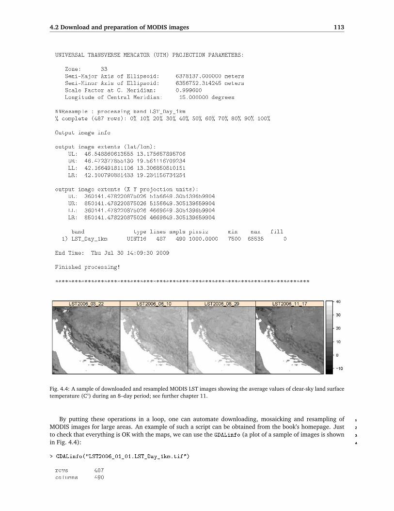
4.2 Download and preparation of MODIS images 113
UNIVERSAL TRANSVERSE MERCATOR (UTM) PROJECTION PARAMETERS:
Zone: 33Semi-Major Axis of Ellipsoid: 6378137.000000 metersSemi-Minor Axis of Ellipsoid: 6356752.314245 metersScale Factor at C. Meridian: 0.999600Longitude of Central Meridian: 15.000000 degrees
NNResample : processing band LST_Day_1km% complete (487 rows): 0% 10% 20% 30% 40% 50% 60% 70% 80% 90% 100%
Output image info-----------------output image extents (lat/lon):
UL: 46.548860613555 13.175657895706UR: 46.472377855130 19.561116709234LL: 42.166491811106 13.306850810151LR: 42.100790881433 19.234156734254
output image extents (X-Y projection units):UL: 360141.478220875026 5156649.305139659904UR: 850141.478220875026 5156649.305139659904LL: 360141.478220875026 4669649.305139659904LR: 850141.478220875026 4669649.305139659904
band type lines smpls pixsiz min max fill1) LST_Day_1km UINT16 487 490 1000.0000 7500 65535 0
End Time: Thu Jul 30 14:09:30 2009
Finished processing!
******************************************************************************
Fig. 4.4: A sample of downloaded and resampled MODIS LST images showing the average values of clear-sky land surfacetemperature (C°) during an 8–day period; see further chapter 11.
By putting these operations in a loop, one can automate downloading, mosaicking and resampling of 1
MODIS images for large areas. An example of such a script can be obtained from the book’s homepage. Just 2
to check that everything is OK with the maps, we can use the GDALinfo (a plot of a sample of images is shown 3
in Fig. 4.4): 4
> GDALinfo("LST2006_01_01.LST_Day_1km.tif")
rows 487columns 490

114 Auxiliary data sources
bands 1origin.x 360641.5origin.y 4669149res.x 1000res.y 1000oblique.x 0oblique.y 0driver GTiffprojection +proj=utm +zone=33 +ellps=WGS84 +datum=WGS84 +units=m +no_defsfile LST2006_01_01.LST_Day_1km.tif
4.3 Summary points1
The availability of remotely sensed data is everyday increasing. Every few years new generation satellites are2
launched that produce images at finer and finer detail, at shorter and shorter revisit time, and with richer3
and richer content (Fig. 4.2). For example, DEMs are now available from a number of sources. Detailed4
and accurate images of topography can now be ordered from remote sensing systems such as SPOT and5
ASTER; SPOT5 offers the High Resolution Stereoscopic (HRS) scanner, which can be used to produce DEMs at6
resolutions of up to 5 m. The cost of data is either free or dropping in price as technology advances. Likewise,7
access to remotely sensed data and various thematic maps is becoming less and less a technical problem —8
live image archives and ordering tools are now available. Multi-source layers are also increasingly compatible9
considering the coverage, scale/resolution, format and metadata description. The intergovernmental Group of10
Earth Observation is building the cyber-infrastructure called GEOSS61 needed to enhance merging of various11
geoinformation layers to a single multi-thematic, multi-purpose data repository. From the time when satellite12
sensors were used for military purposes only, we now live in an era when anybody can load high resolution13
images of earth and detailed digital maps to their computer.14
In the context of geostatistical mapping, the number of possible covariates is today increasing dramatically,15
so that there is practically no reason any more to study point-sampled variables in relation to its spatial coor-16
dinates only (Pebesma, 2006). External variables should be used wherever possible to improve geostatistical17
mapping. Majority of global spatial layers are today available at no cost at resolutions 1–10 km (see the world18
maps repository); MODIS imagery is freely available at resolution of 250 m; global elevation data is available19
at resolutions of 60–90 m; archive Landsat images (15–30 m) can be obtained for most of the world. All20
this proves that there is no reason not to use auxiliary covariates (i.e. methods such as regression-kriging) for21
geostatistical mapping.22
In this chapter, I have specifically put an emphasis on MODIS products, mainly because the images are23
relatively easy to obtain for various parts of the world (or globally), and because MODIS images are valuable24
for monitoring ecosystem dynamics. From the aspect of ecology and nature conservation, the importance of25
MODIS images for environmental management and nature conservation is enormous (Lunetta et al., 2006).26
They can be obtained by anybody at any time and can be used as an independent source of information to27
quantify degradation of natural systems that is possibly not visible using local sources of information. MODIS28
EVI images can be used to show changes in land cover, deforestation, damage caused by global warming or29
even fine long-term succession processes. Because MODIS EVI is available from year the 2000, anybody can30
compare the current situation with the situation from a decade ago. The script presented can be obtained form31
the book’s homepage and adopted to download any type of MODIS products available from the USGS Land32
Processes Distributed Active Archive Center.33
The next generation remote sensing systems/surveys will certainly be multi-thematic and based on active34
surface-penetrating sensors. The future of automated mapping lays in using technologies such as LiDAR in35
combination with other optical, radar and hyperspectral sensors. This type of multi-thematic imagery will36
enable analysts to represent both surface and sub-surface properties of objects of interest, so that none of37
the important characteristics are overlooked. Multi-thematic scanners should also make the airborne surveys38
cheaper and hence suited for local and regional scale environmental studies.39
61http://www.earthobservations.org

4.3 Summary points 115
Further reading: 1
Æ Doll, C.N.H., Muller, J.-P., Morley, J.G. 2007. Mapping regional economic activity from night-time light 2
satellite imagery. Ecological Economics, 57(1): 75–92. 3
Æ Hijmans, R.J., Cameron, S.E., Parra, J.L., Jones, P.G., Jarvis, A., 2005. Very high resolution interpolated 4
climate surfaces for global land areas. International Journal of Climatology 25: 1965–1978. 5
Æ Pebesma, E.J., 2006. The Role of External Variables and GIS Databases in Geostatistical Analysis. Trans- 6
actions in GIS, 10(4): 615–632. 7
Æ http://www.fao.org/geonetwork/srv/en/main.home — FAO’s GeoNetwork server. 8
Æ http://www.geoportal.org/web/guest/geo_image_gallery — ESA’s GeoPortal gallery. 9
Æ http://geodata.grid.unep.ch/ — UNEP/GRID GEO DataPortal. 10
Æ http://neo.sci.gsfc.nasa.gov/ — NASA’s Earth Observation (NEO) portal. 11
Æ http://glcf.umiacs.umd.edu/portal/geocover/ — Global Land Cover Facility (GLCF) geopor- 12
tal operated by the University of Maryland. 13
Æ https://lpdaac.usgs.gov/lpdaac/ — Land Processes Distributed Active Archive Center (distrib- 14
utor of MODIS products). 15

116 Auxiliary data sources

5 1
First steps (meuse) 2
5.1 Introduction 3
This exercise introduces geostatistical tools that can be used to analyze various types of environmental data. It 4
is not intended as a complete analysis of the example data set. Indeed some of the steps here can be questioned, 5
expanded, compared, and improved. The emphasis is on seeing what R and some of its add-in packages can 6
do in combination with an open source GIS such as SAGA GIS. The last section demonstrates how to export 7
produced maps to Google Earth. This whole chapter is, in a way, a prerequisite to other exercises in the book. 8
We will use the meuse data set, which is a classical geostatistical data set used frequently by the creator of 9
the gstat package to demonstrate various geostatistical analysis steps (Bivand et al., 2008, §8). The data set is 10
documented in detail by Rikken and Van Rijn (1993), and Burrough and McDonnell (1998). It consists of 155 11
samples of top soil heavy metal concentrations (ppm), along with a number of soil and landscape variables. 12
The samples were collected in a flood plain of the river Meuse, near the village Stein (Lat. 50° 58’ 16", Long. 13
5° 44’ 39"). Historic metal mining has caused the widespread dispersal of lead, zinc, copper and cadmium 14
in the alluvial soil. The pollutants may constrain the land use in these areas, so detailed maps are required 15
that identify zones with high concentrations. Our specific objective will be to generate a map of a heavy metal 16
(zinc) in soil, and a map of soil liming requirement (binary variable) using point observations, and a range of 17
auxiliary maps. 18
Upon completion of this exercise, you will be able to plot and fit variograms, examine correlation between 19
various variables, run spatial predictions using the combination of continuous and categorical predictors and 20
visualize results in external GIS packages/browsers (SAGA GIS, Google Earth). If you are new to R syntax, 21
you should consider first studying some of the introductory books (listed in the section 3.4.2). 22
5.2 Data import and exploration 23
Download the attached meuse.R script from the book’s homepage and open it in Tinn-R. First, open a new 24
R session and change the working directory to where all your data sets will be located (C:/meuse/). This 25
directory will be empty at the beginning, but you will soon be able to see data sets that you will load, generate 26
and/or export. Now you can run the script line by line. Feel free to experiment with the code and extend it as 27
needed. Make notes if you experience any problems or if you are not able to perform some operation. 28
Before you start processing the data, you will need to load the following packages: 29
> library(maptools)> library(gstat)> library(rgdal)> library(lattice)> library(RSAGA)> library(geoR)> library(spatstat)
117

118 First steps (meuse)
You can get a list of methods in each package with the help method, e.g.:1
> help(package="maptools")
The meuse data set is in fact available in the installation directory of the gstat package. You can load the2
field observations by typing:3
> data(meuse)> str(meuse)
'data.frame': 155 obs. of 14 variables:$ x : num 181072 181025 181165 181298 181307 ...$ y : num 333611 333558 333537 333484 333330 ...$ cadmium: num 11.7 8.6 6.5 2.6 2.8 3 3.2 2.8 2.4 1.6 ...$ copper : num 85 81 68 81 48 61 31 29 37 24 ...$ lead : num 299 277 199 116 117 137 132 150 133 80 ...$ zinc : num 1022 1141 640 257 269 ...$ elev : num 7.91 6.98 7.80 7.66 7.48 ...$ dist : num 0.00136 0.01222 0.10303 0.19009 0.27709 ...$ om : num 13.6 14 13 8 8.7 7.8 9.2 9.5 10.6 6.3 ...$ ffreq : Factor w/ 3 levels "1","2","3": 1 1 1 1 1 1 1 1 1 1 ...$ soil : Factor w/ 3 levels "1","2","3": 1 1 1 2 2 2 2 1 1 2 ...$ lime : Factor w/ 2 levels "0","1": 2 2 2 1 1 1 1 1 1 1 ...$ landuse: Factor w/ 15 levels "Aa","Ab","Ag",..: 4 4 4 11 4 11 4 2 2 15 ...$ dist.m : num 50 30 150 270 380 470 240 120 240 420 ...
Zn
meuse$zinc
Fre
quen
cy
500 1000 1500
05
1015
2025
Fig. 5.1: Histogram plot for zinc (meuse data set).
which shows a table with 155 observations of 14 variables.4
To get a complete description of this data set, type:5
> ?meuse
Help for 'meuse' is shown in the browser
which will open your default web-browser and show the6
Html help page for this data set. Here you can also find7
what the abbreviated names for the variables mean. We8
will focus on mapping the following two variables: zinc9
— topsoil zinc concentration in ppm; and lime — the log-10
ical variable indicating whether the soil needs liming or11
not.12
Now we can start to visually explore the data set. For13
example, we can visualize the target variable with a his-14
togram:15
> hist(meuse$zinc, breaks=25, col="grey")
which shows that the target variable is skewed towards16
lower values (Fig. 5.1), and it needs to be transformed17
before we can run any linear interpolation.18
To be able to use spatial operations in R e.g. from the19
gstat package, we must convert the imported table into a SpatialPointDataFrame, a point map (with at-20
tributes), using the coordinates method:21
# 'attach coordinates' - convert table to a point map:> coordinates(meuse) <- ∼ x+y> str(meuse)
Formal class 'SpatialPointsDataFrame' [package "sp"] with 5 slots..@ data :'data.frame': 155 obs. of 12 variables:.. ..$ cadmium: num [1:155] 11.7 8.6 6.5 2.6 2.8 3 3.2 2.8 2.4 1.6 ..... ..$ copper : num [1:155] 85 81 68 81 48 61 31 29 37 24 ...

5.2 Data import and exploration 119
.. ..$ lead : num [1:155] 299 277 199 116 117 137 132 150 133 80 ...
.. ..$ zinc : num [1:155] 1022 1141 640 257 269 ...
.. ..$ elev : num [1:155] 7.91 6.98 7.80 7.66 7.48 ...
.. ..$ dist : num [1:155] 0.00136 0.01222 0.10303 0.19009 0.27709 ...
.. ..$ om : num [1:155] 13.6 14 13 8 8.7 7.8 9.2 9.5 10.6 6.3 ...
.. ..$ ffreq : Factor w/ 3 levels "1","2","3": 1 1 1 1 1 1 1 1 1 1 ...
.. ..$ soil : Factor w/ 3 levels "1","2","3": 1 1 1 2 2 2 2 1 1 2 ...
.. ..$ lime : Factor w/ 2 levels "0","1": 2 2 2 1 1 1 1 1 1 1 ...
.. ..$ landuse: Factor w/ 15 levels "Aa","Ab","Ag",..: 4 4 4 11 4 11 4 2 2 15 ...
.. ..$ dist.m : num [1:155] 50 30 150 270 380 470 240 120 240 420 ...
..@ coords.nrs : int [1:2] 1 2
..@ coords : num [1:155, 1:2] 181072 181025 181165 181298 181307 ...
.. ..- attr(*, "dimnames")=List of 2
.. .. ..$ : NULL
.. .. ..$ : chr [1:2] "x" "y"
..@ bbox : num [1:2, 1:2] 178605 329714 181390 333611
.. ..- attr(*, "dimnames")=List of 2
.. .. ..$ : chr [1:2] "x" "y"
.. .. ..$ : chr [1:2] "min" "max"
..@ proj4string:Formal class 'CRS' [package "sp"] with 1 slots
.. .. ..@ projargs: chr NA
Note that the structure is now more complicated, with a nested structure and 5 ‘slots’1 (Bivand et al., 2008, 1
§2): 2
(1.) @data contains the actual data in a table format (a copy of the original dataframe minus the coordinates); 3
(2.) @coords.nrs has the coordinate dimensions; 4
(3.) @coords contains coordinates of each element (point); 5
(4.) @bbox stands for ‘bounding box’ — this was automatically estimated by sp; 6
(5.) @proj4string contains the definition of projection system following the proj42 format. 7
The projection and coordinate system are at first unknown (listed as NA meaning ‘not applicable’). Coordi- 8
nates are just numbers as far as it is concerned. We know from the data set producers that this map is in the 9
so-called “Rijksdriehoek” or RDH (Dutch triangulation), which is extensively documented3. This is a: 10
stereographic projection (parameter +proj); 11
on the Bessel ellipsoid (parameter +ellps); 12
with a fixed origin (parameters +lat_0 and +lon_0); 13
scale factor at the tangency point (parameter +k); 14
the coordinate system has a false origin (parameters +x_0 and +y_0); 15
the center of the ellipsoid is displaced with respect to the standard WGS84 ellipsoid (parameter +towgs84, 16
with three distances, three angles, and one scale factor)4; 17
It is possible to specify all this information with the CRS method; however, it can be done more simply if 18
the datum is included in the European Petroleum Survey Group (EPSG) database5, now maintained by the 19
International Association of Oil & Gas producers (OGP). This database is included as text file (epsg) in the 20
rgdal package, in the subdirectory library/rgdal/proj in the R installation folder. Referring to the EPSG 21
registry6, we find the following entry: 22
1This is the S4 objects vocabulary. Slots are components of more complex objects.2http://trac.osgeo.org/proj/3http://www.rdnap.nl4The so-called seven datum transformation parameters (translation + rotation + scaling); also known as the Bursa Wolf method.5http://www.epsg-registry.org/6http://spatialreference.org/ref/epsg/28992/

120 First steps (meuse)
# Amersfoort / RD New <28992> +proj=sterea +lat_0=52.15616055555555+lon_0=5.38763888888889 +k=0.999908 +x_0=155000 +y_0=463000 +ellps=bessel+towgs84=565.237,50.0087,465.658,-0.406857,0.350733,-1.87035,4.0812+units=m +no_defs <>
This shows that the Amersfoort / RD New system is EPSG reference 28992. Note that some older instal-1
lations of GDAL do not carry the seven-transformation parameters that define the geodetic datum! Hence,2
you will need to add these parameters manually to your library/rgdal/proj/epsg file. Once you have set3
the correct parameters in the system, you can add the projection information to this data set using the CRS4
method:5
> proj4string(meuse) <- CRS("+init=epsg:28992")> meuse@proj4string
CRS arguments:+init=epsg:28992 +proj=sterea +lat_0=52.15616055555555+lon_0=5.38763888888889 +k=0.9999079 +x_0=155000 +y_0=463000 +ellps=bessel+towgs84=565.237,50.0087,465.658,-0.406857,0.350733,-1.87035,4.0812+units=m +no_defs
so now the correct projection information is included in the proj4string slot and we will be able to transform6
this spatial layer to geographic coordinates, and then export and visualize further in Google Earth.7
Once we have converted the table to a point map we can proceed with spatial exploration data analysis,8
e.g. we can simply plot the target variable in relation to sampling locations. A common plotting scheme used9
to display the distribution of values is the bubble method. In addition, we can import also a map of the river,10
and then display it together with the values of zinc (Bivand et al., 2008):11
# load river (lines):> data(meuse.riv)# convert to a polygon map:> tmp <- list(Polygons(list(Polygon(meuse.riv)), "meuse.riv"))> meuse.riv <- SpatialPolygons(tmp)> class(meuse.riv)
[1] "SpatialPolygons"attr(,"package")[1] "sp"
> proj4string(meuse.riv) <- CRS("+init=epsg:28992")# plot together points and river:> bubble(meuse, "zinc", scales=list(draw=T), col="black", pch=1, maxsize=1.5,+ sp.layout=list("sp.polygons", meuse.riv, col="grey"))
which will produce the plot shown in Fig. 5.2, left7. Alternatively, you can also export the meuse data set to12
ESRI Shapefile format:13
> writeOGR(meuse, ".", "meuse", "ESRI Shapefile")
which will generate four files in your working directory: meuse.shp (geometry), meuse.shx (auxiliary file),14
meuse.dbf (table with attributes), and meuse.prj (coordinate system). This shapefile you can now open in15
SAGA GIS and display using the same principle as with the bubble method (Fig. 5.2, right). Next, we import16
the gridded maps (40 m resolution). We will load them from the web repository8:17
# download the gridded maps:> setInternet2(use=TRUE) # you need to login on the book's homepage first!> download.file("http://spatial-analyst.net/book/system/files/meuse.zip",+ destfile=paste(getwd(), "meuse.zip", sep="/"))> grid.list <- c("ahn.asc", "dist.asc", "ffreq.asc", "soil.asc")
7See also http://r-spatial.sourceforge.net/gallery/ for a gallery of plots using meuse data set.8This has some extra layers compared to the existing meusegrid data set that comes with the sp package.

5.2 Data import and exploration 121
zinc
330000
331000
332000
333000
178500 179500 180500 181500
●●● ●
●●
●●●
●●
●
●●●
●●
●●
●●●●
●●●●
●●
●
●●●
●●●
●●●●●
●●
●
●●●●
●
●●
●●●●●●
●●
●●●●
●●
●●
●
●●●●
●●●●●
●●●●
●
●
●
●
●
●●
●
● ●●●
●●
●
●●●
●●
●
●
●
●
●
●
●
●
●●
●
●
●●
●
●
●
●
●
●●
●●
●
●
●
●
●
●
●
●
●
●
●
●
●
●●●
● ●
●
●●
●●●
●
●
●
●●●
●
●
●
●
●
●
113198326674.51839
Fig. 5.2: Meuse data set and values of zinc (ppm): visualized in R (left), and in SAGA GIS (right).
# unzip the maps in a loop:> for(j in grid.list){> fname <- zip.file.extract(file=j, zipname="meuse.zip")> file.copy(fname, paste("./", j, sep=""), overwrite=TRUE)> }
These are the explanatory variables that we will use to improve spatial prediction of the two target vari- 1
ables: 2
(1.) ahn — digital elevation model (in cm) obtained from the LiDAR survey of the Netherlands9; 3
(2.) dist — distance to river Meuse (in metres). 4
(3.) ffreq — flooding frequency classes: (1) high flooding frequency, (2) medium flooding frequency, (3) 5
no flooding; 6
(4.) soil — map showing distribution of soil types, following the Dutch classification system: (1) Rd10A, 7
(2) Rd90C-VIII, (3) Rd10C (de Fries et al., 2003); 8
In addition, we can also unzip the 2 m topomap that we can use as the background for displays (Fig. 5.2, 9
right): 10
# the 2 m topomap:> fname <- zip.file.extract(file="topomap2m.tif", zipname="meuse.zip")> file.copy(fname, "./topomap2m.tif", overwrite=TRUE)
We can load the grids to R, also by using a loop operation: 11
> meuse.grid <- readGDAL(grid.list[1])
ahn.asc has GDAL driver AAIGridand has 104 rows and 78 columns
9http://www.ahn.nl
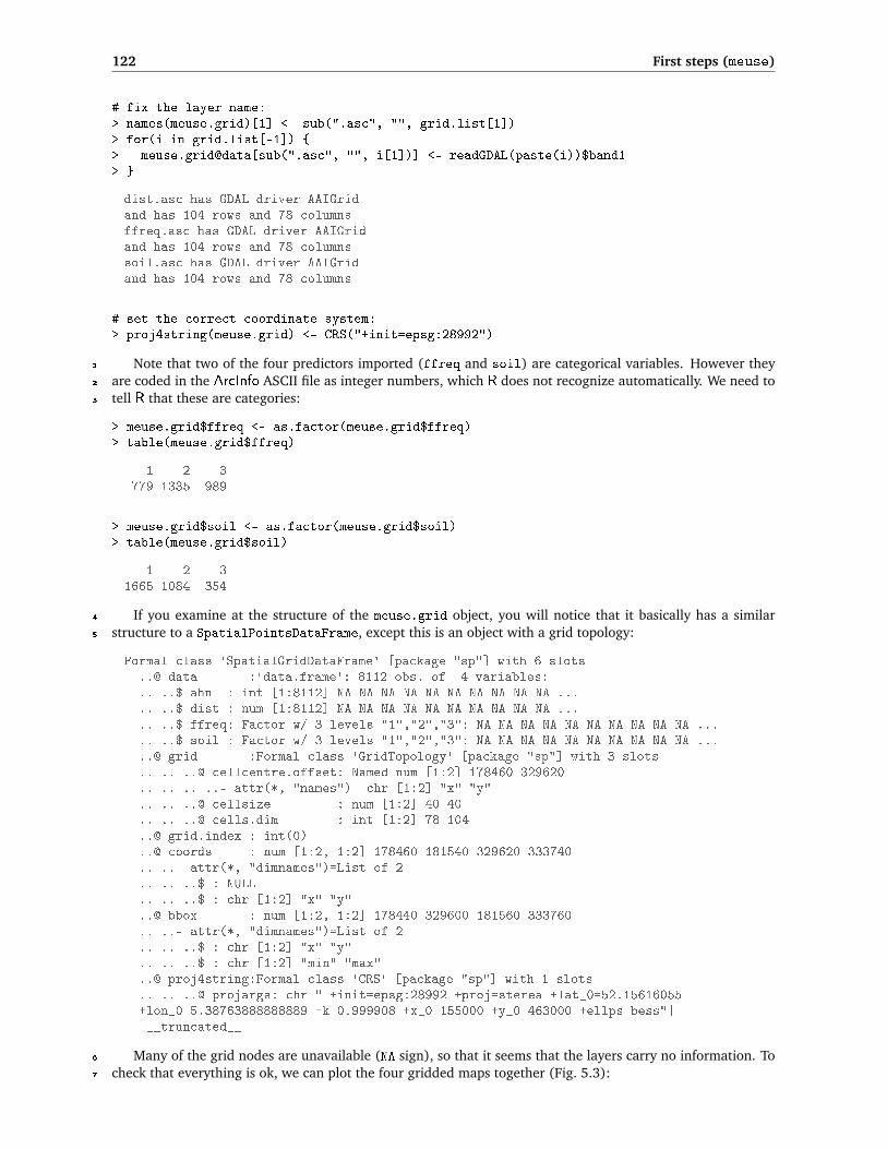
122 First steps (meuse)
# fix the layer name:> names(meuse.grid)[1] <- sub(".asc", "", grid.list[1])> for(i in grid.list[-1]) {> meuse.grid@data[sub(".asc", "", i[1])] <- readGDAL(paste(i))$band1> }
dist.asc has GDAL driver AAIGridand has 104 rows and 78 columnsffreq.asc has GDAL driver AAIGridand has 104 rows and 78 columnssoil.asc has GDAL driver AAIGridand has 104 rows and 78 columns
# set the correct coordinate system:> proj4string(meuse.grid) <- CRS("+init=epsg:28992")
Note that two of the four predictors imported (ffreq and soil) are categorical variables. However they1
are coded in the ArcInfo ASCII file as integer numbers, which R does not recognize automatically. We need to2
tell R that these are categories:3
> meuse.grid$ffreq <- as.factor(meuse.grid$ffreq)> table(meuse.grid$ffreq)
1 2 3779 1335 989
> meuse.grid$soil <- as.factor(meuse.grid$soil)> table(meuse.grid$soil)
1 2 31665 1084 354
If you examine at the structure of the meuse.grid object, you will notice that it basically has a similar4
structure to a SpatialPointsDataFrame, except this is an object with a grid topology:5
Formal class 'SpatialGridDataFrame' [package "sp"] with 6 slots..@ data :'data.frame': 8112 obs. of 4 variables:.. ..$ ahn : int [1:8112] NA NA NA NA NA NA NA NA NA NA ..... ..$ dist : num [1:8112] NA NA NA NA NA NA NA NA NA NA ..... ..$ ffreq: Factor w/ 3 levels "1","2","3": NA NA NA NA NA NA NA NA NA NA ..... ..$ soil : Factor w/ 3 levels "1","2","3": NA NA NA NA NA NA NA NA NA NA .....@ grid :Formal class 'GridTopology' [package "sp"] with 3 slots.. .. ..@ cellcentre.offset: Named num [1:2] 178460 329620.. .. .. ..- attr(*, "names")= chr [1:2] "x" "y".. .. ..@ cellsize : num [1:2] 40 40.. .. ..@ cells.dim : int [1:2] 78 104..@ grid.index : int(0)..@ coords : num [1:2, 1:2] 178460 181540 329620 333740.. ..- attr(*, "dimnames")=List of 2.. .. ..$ : NULL.. .. ..$ : chr [1:2] "x" "y"..@ bbox : num [1:2, 1:2] 178440 329600 181560 333760.. ..- attr(*, "dimnames")=List of 2.. .. ..$ : chr [1:2] "x" "y".. .. ..$ : chr [1:2] "min" "max"..@ proj4string:Formal class 'CRS' [package "sp"] with 1 slots.. .. ..@ projargs: chr " +init=epsg:28992 +proj=sterea +lat_0=52.15616055+lon_0=5.38763888888889 +k=0.999908 +x_0=155000 +y_0=463000 +ellps=bess"|__truncated__
Many of the grid nodes are unavailable (NA sign), so that it seems that the layers carry no information. To6
check that everything is ok, we can plot the four gridded maps together (Fig. 5.3):7

5.2 Data import and exploration 123
ffreq.plt <- spplot(meuse.grid["ffreq"],+ col.regions=grey(runif(length(levels(meuse.grid$ffreq)))),+ main="Flooding frequency classes")dist.plt <- spplot(meuse.grid["dist"],+ col.regions=grey(rev(seq(0,1,0.025))),+ main="Distance to river")soil.plt <- spplot(meuse.grid["soil"],+ col.regions=grey(runif(length(levels(meuse.grid$ffreq)))),+ main="Soil type classes")ahn.plt <- spplot(meuse.grid["ahn"],+ col.regions=grey(rev(seq(0,1,0.025))),+ main="Elevation (cm)")> print(ffreq.plt, split=c(1, 1, 4, 1), more=TRUE)> print(dist.plt, split=c(2, 1, 4, 1), more=TRUE)> print(ahn.plt, split=c(3, 1, 4, 1), more=TRUE)> print(soil.plt, split=c(4, 1, 4, 1), more=TRUE)
Flooding frequency classes
123
Distance to river
0.0
0.2
0.4
0.6
0.8
1.0
Elevation (cm)
3000
3500
4000
4500
5000
5500
6000
Soil type classes
123
Fig. 5.3: Meuse auxiliary predictors.
5.2.1 Exploratory data analysis: sampling design 1
As noted in the preface, no geostatistician can promise high quality products without quality input point 2
samples. To assess how representative and consistent the input data are, we can run some basic exploratory 3
analysis to look at the point geometry and how well the environmental features are represented. We can start 4
with point pattern analysis as implemented in the spatstat package, e.g. to determine the average spacing 5
between the points (Baddeley, 2008): 6
# coerce to a ppp object:> mg_owin <- as.owin(meuse.grid["dist"])> meuse.ppp <- ppp(x=coordinates(meuse)[,1], y=coordinates(meuse)[,2],+ marks=meuse$zinc, window=mg_owin)# plot(meuse.ppp)> summary(dist.points)
Min. 1st Qu. Median Mean 3rd Qu. Max.43.93 77.88 107.40 111.70 137.70 353.00
which shows that the means shortest distance is 111 m. The following two questions are relevant for further 7
analysis: (1) are the sampling locations distributed independently and uniformly over the area of interest 8
(i.e. is there a significant clustering of locations)? (2) is the environmental feature space well represented? To 9
answer the first question we can test the sampling design for Complete Spatial Randomness (CSR). CRS assumes 10
that there are no regions in the study area where events are more likely to occur, and that the presence of a 11
given event does not modify the probability of other events appearing nearby (Bivand et al., 2008). 12
The compatibility of a sampling design with CRS can be assessed by plotting the empirical function against 13
the theoretical expectation (Bivand et al., 2008, p.160–163): 14
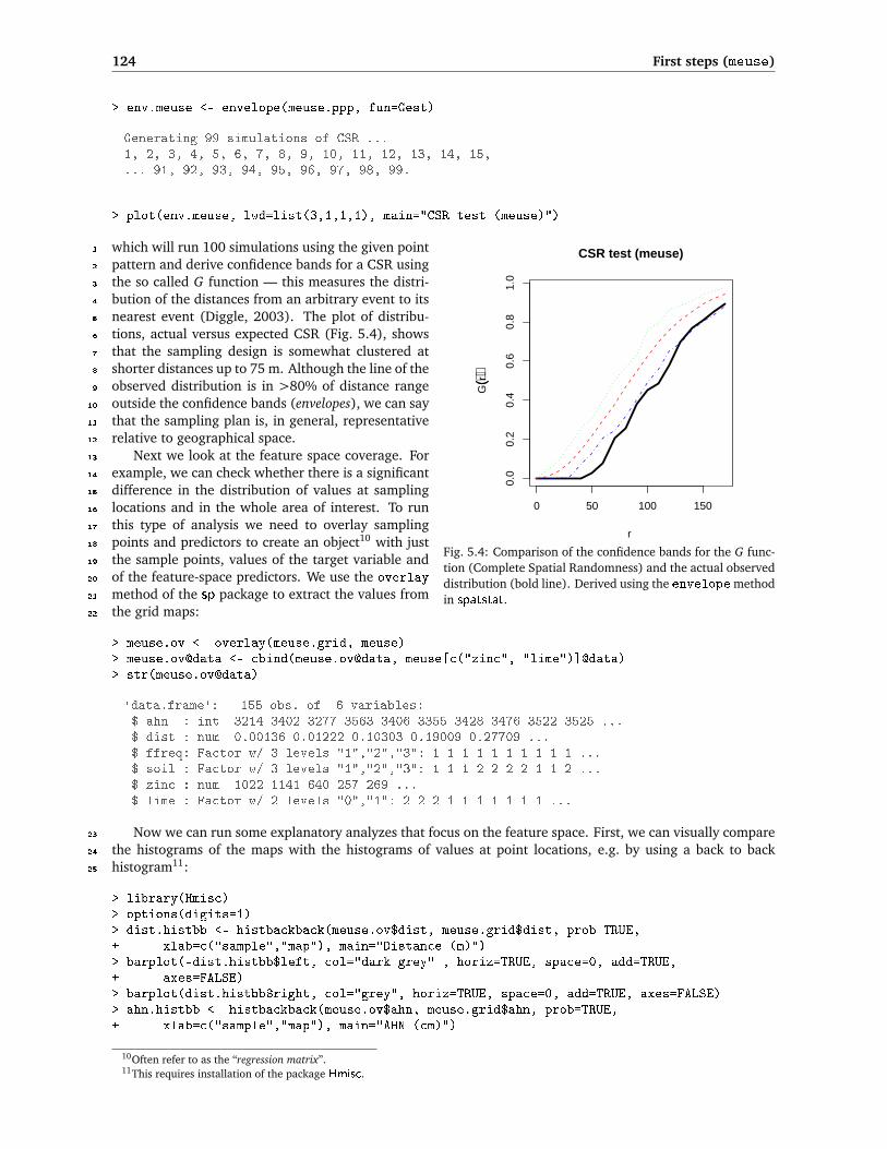
124 First steps (meuse)
> env.meuse <- envelope(meuse.ppp, fun=Gest)
Generating 99 simulations of CSR ...1, 2, 3, 4, 5, 6, 7, 8, 9, 10, 11, 12, 13, 14, 15,... 91, 92, 93, 94, 95, 96, 97, 98, 99.
> plot(env.meuse, lwd=list(3,1,1,1), main="CSR test (meuse)")
0 50 100 1500.
00.
20.
40.
60.
81.
0
CSR test (meuse)
r
G((r))
Fig. 5.4: Comparison of the confidence bands for the G func-tion (Complete Spatial Randomness) and the actual observeddistribution (bold line). Derived using the envelope methodin spatstat.
which will run 100 simulations using the given point1
pattern and derive confidence bands for a CSR using2
the so called G function — this measures the distri-3
bution of the distances from an arbitrary event to its4
nearest event (Diggle, 2003). The plot of distribu-5
tions, actual versus expected CSR (Fig. 5.4), shows6
that the sampling design is somewhat clustered at7
shorter distances up to 75 m. Although the line of the8
observed distribution is in >80% of distance range9
outside the confidence bands (envelopes), we can say10
that the sampling plan is, in general, representative11
relative to geographical space.12
Next we look at the feature space coverage. For13
example, we can check whether there is a significant14
difference in the distribution of values at sampling15
locations and in the whole area of interest. To run16
this type of analysis we need to overlay sampling17
points and predictors to create an object10 with just18
the sample points, values of the target variable and19
of the feature-space predictors. We use the overlay20
method of the sp package to extract the values from21
the grid maps:22
> meuse.ov <- overlay(meuse.grid, meuse)> meuse.ov@data <- cbind(meuse.ov@data, meuse[c("zinc", "lime")]@data)> str(meuse.ov@data)
'data.frame': 155 obs. of 6 variables:$ ahn : int 3214 3402 3277 3563 3406 3355 3428 3476 3522 3525 ...$ dist : num 0.00136 0.01222 0.10303 0.19009 0.27709 ...$ ffreq: Factor w/ 3 levels "1","2","3": 1 1 1 1 1 1 1 1 1 1 ...$ soil : Factor w/ 3 levels "1","2","3": 1 1 1 2 2 2 2 1 1 2 ...$ zinc : num 1022 1141 640 257 269 ...$ lime : Factor w/ 2 levels "0","1": 2 2 2 1 1 1 1 1 1 1 ...
Now we can run some explanatory analyzes that focus on the feature space. First, we can visually compare23
the histograms of the maps with the histograms of values at point locations, e.g. by using a back to back24
histogram11:25
> library(Hmisc)> options(digits=1)> dist.histbb <- histbackback(meuse.ov$dist, meuse.grid$dist, prob=TRUE,+ xlab=c("sample","map"), main="Distance (m)")> barplot(-dist.histbb$left, col="dark grey" , horiz=TRUE, space=0, add=TRUE,+ axes=FALSE)> barplot(dist.histbb$right, col="grey", horiz=TRUE, space=0, add=TRUE, axes=FALSE)> ahn.histbb <- histbackback(meuse.ov$ahn, meuse.grid$ahn, prob=TRUE,+ xlab=c("sample","map"), main="AHN (cm)")
10Often refer to as the “regression matrix”.11This requires installation of the package Hmisc.

5.2 Data import and exploration 125
> barplot(-ahn.histbb$left, col="dark grey" , horiz=TRUE, space=0, add=TRUE,+ axes=FALSE)> barplot(ahn.histbb$right, col="grey", horiz=TRUE, space=0, add=TRUE, axes=FALSE)> par(mfrow=c(1,2))> print(dist.histbb, add=TRUE)> print(ahn.histbb, add=FALSE)> dev.off()> options(digits=3)
Distance (m)Distance (m)
4 3 2 1 0 1 2 3
0.0
0.2
0.4
0.6
0.8
1.0
sample map
AHN (cm)AHN (cm)
0.003 0.002 0.001 0.000 0.001 0.00228
00.0
3800
.048
00.0
5800
.0
sample map
Fig. 5.5: Histogram for sampled values of dist and ahn (155 locations) versus the histogram of the raster map (all rasternodes). Produced using the histbackback method.
This will produce two histograms next to each other so that we can visually compare how well the samples 1
represent the original feature space of the raster maps (Fig. 5.5). In the case of the points data set, we can 2
see that the samples are misrepresenting higher elevations, but distances from the river are well represented. 3
We can actually test if the histograms of sampled variables are significantly different from the histograms of 4
original raster maps e.g. by using a non-parametric test such as the Kolmogorov-Smirnov test: 5
> ks.test(dist.histbb$left, dist.histbb$right)
Two-sample Kolmogorov-Smirnov test
data: dist.histbb$left and dist.histbb$rightD = 0.2, p-value = 0.9945alternative hypothesis: two-sided
> ks.test(ahn.histbb$left, ahn.histbb$right)
Two-sample Kolmogorov-Smirnov test
data: ahn.histbb$left and ahn.histbb$rightD = 0.7, p-value = 0.0001673alternative hypothesis: two-sided
Warning message:In ks.test(ahn.histbb$left, ahn.histbb$right) :
cannot compute correct p-values with ties
which shows that the first two histograms (dist) do not differ much, but the second two (ahn) have signif- 6
icantly different distributions (D=0.7, p-value=0.0001673). Another test that you might do to compare the 7
histograms is to run the correlation test12: 8
12Also known as the test of no correlation because it computes t-value for correlation coefficient being equal to zero.

126 First steps (meuse)
> cor.test(ahn.histbb$left, ahn.histbb$right)
In the step of geographic analysis of the sampling design we will assess whether the sampling density1
within different soil mapping units (soil) is consistent. First, we look at how many points fall into each zone:2
> summary(meuse.ov$soil)
1 2 397 46 12
then we need to derive the observed inspection density using:3
# observed:> inspdens.obs <- summary(meuse.ov$soil)[1:length(levels(meuse.ov$soil))]/+ (summary(meuse.grid$soil)[1:length(levels(meuse.grid$soil))]+ *meuse.grid@grid@cellsize[[1]]^2)# expected:> inspdens.exp <- rep(length(meuse.ov$soil)/+ (length(meuse.grid$soil[!is.na(meuse.grid$soil)])+ *meuse.grid@grid@cellsize[[1]]^2), length(levels(meuse.ov$soil)))# inspection density in no./ha:> inspdens.obs*10000
1 2 30.364 0.265 0.212
> inspdens.exp*10000
[1] 0.312 0.312 0.312
which can also be compared by using the Kolmogorov-Smirnov test:4
> ks.test(inspdens.obs, inspdens.exp)
Two-sample Kolmogorov-Smirnov test
data: inspdens.obs and inspdens.expD = 0.667, p-value = 0.5176alternative hypothesis: two-sided
Warning message:In ks.test(inspdens.obs, inspdens.exp) :cannot compute correct p-values with ties
In this case, we see that inspection density is also significantly inconsistent considering the map of soil,5
which is not by chance (p-value=0.5176). We could also run a similar analysis for land cover types or any6
other factor-type predictors.7
So in summary, we can conclude for the meuse sampling design that:8
the average distance to the nearest neighbor is 111 m and the size of the area is 496 ha;9
the sampling intensity is 3 points per 10 ha, which corresponds to a grid cell size of about 15 m (Hengl,10
2006);11
the sampling density varies in geographical space — sampling is significantly clustered for smaller dis-12
tance (<75 m);13
the sampling is unrepresentative considering the maps of ahn and soil — higher elevations and soil14
class 3 are significantly under-sampled;15
These results do not mean that this data set is unsuitable for generating maps, but they do indicate that it16
has some limitations considering representativeness, independency and consistency requirements.17

5.3 Zinc concentrations 127
5.3 Zinc concentrations 1
5.3.1 Regression modeling 2
The main objective of regression-kriging analysis is to build a regression model by using the explanatory 3
gridded maps. We have previously estimated values of explanatory maps and target variables in the same 4
table (overlay operation), so we can start by visually exploring the relation between the target variable and 5
the continuous predictors e.g. by using a smoothed scatterplot (Fig. 5.6): 6
> par(mfrow = c(1, 2))> scatter.smooth(meuse.ov$dist, meuse.ov$zinc, span=18/19,+ col="grey", xlab="Distance to river (log)", ylab="Zinc (ppm)")> scatter.smooth(meuse.ov$ahn, meuse.ov$zinc, span=18/19,+ col="grey", xlab="Elevation (cm)", ylab="Zinc (ppm)")
which shows that the values of zinc decrease as the distance from (water) streams and elevation increases. 7
This supports our knowledge about the area — the majority of heavy metals has been originated from fresh 8
water deposition. The relation seems to be particulary clear, but it appears to be non-linear as the fitted lines 9
are curved. 10
●
●
●
● ● ●●
●●
●●●
●
●
●
●
●
●●
●
●
●●
● ● ●●●●
●●●●
●●
●
●
●●
●
●
●●●
● ●
●●
●●
●
●
●
●
●
●
●
●
●
●
●
●●●
●●
●
●
●● ●
●
●●●
●
●●
●
●
●
●
●
●●●
●●●
●●
●●
●●
●●●● ●●
●●
● ● ● ●●●●●
●●●●● ●
●
●●●
●
●
●
●
● ● ●
●●
●●●
●●● ●●
●
●
●●●
●●
● ●
●
●●
●
●
●
●
●
0.0 0.2 0.4 0.6 0.8
500
1000
1500
Distance to river (log)
Zin
c (p
pm)
●
●
●
●●●●
●●
●●●
●
●
●
●
●
●●
●
●
●●
●●●●●●
● ●●●●●
●
●
●●
●
●
●●●
●●
●●
●●
●
●
●
●
●
●
●
●
●
●
●
●●●
●●
●
●
●●●
●
●●●
●
●●
●
●
●
●
●
● ●●
●●●●●
●●
●●
●●● ● ●●
●●
●●● ●●●
●●● ●●●
● ●
●
●●●
●
●
●
●
● ●●
●●
●●●
● ●●●●
●
●
●●●
●●
●●
●
●●
●
●
●
●
●
3200 3400 3600 3800
500
1000
1500
Elevation (cm)
Zin
c (p
pm)
Fig. 5.6: Scatterplots showing the relation between zinc and distance from river, and elevation.
Another useful analysis relevant for the success of regression modeling is to look at the multicolinearity of 11
predictors. Some predictors show the same feature, i.e. they are not independent. For example, dist.asc and 12
ahn.asc maps are correlated: 13
> pairs(zinc ∼ ahn+dist, meuse.ov)> cor(meuse.grid$ahn, meuse.grid$dist, use="complete.obs")
[1] 0.294
To visualize the relationship between the target variable and the classified predictors we used a grouped 14
boxplot; this also allows us to count the samples in each class (Fig. 5.7): 15
> par(mfrow=c(1,2))> boxplot(log1p(meuse.ov$zinc) ∼ meuse.ov$soil,+ col=grey(runif(length(levels(meuse.ov$soil)))),+ xlab="Soil type classes", ylab="Zinc (ppm)")> boxplot(log1p(meuse.ov$zinc) ∼ meuse.ov$ffreq,+ col=grey(runif(length(levels(meuse.ov$soil)))),+ xlab="Flooding frequency classes", ylab="Zinc (ppm)")> dev.off()> boxplot(log1p(meuse.ov$zinc) ∼ meuse.ov$soil, plot=FALSE)$n

128 First steps (meuse)
●
●●●
1 2 3
5.0
5.5
6.0
6.5
7.0
7.5
Soil type classes
Zin
c (p
pm)
1 2 3
5.0
5.5
6.0
6.5
7.0
7.5
Flooding frequency classes
Zin
c (p
pm)
Fig. 5.7: Boxplots showing differences in zinc values (log-scale) between various soil and flooding frequency mappingunits.
[1] 97 46 12
> boxplot(log1p(meuse.ov$zinc) ∼ meuse.ov$ffreq, plot=FALSE)$n
[1] 73 53 29
which indicates that soil class "1" carries significantly higher zinc content than the remaining two classes.1
Note that there are only 12 field samples in the soil class "3", but still enough13 to fit a regression model.2
Now that we have some idea of the qualitative relation between the predictors and target variable, we3
proceed with fitting a regression model. We will first try to explain variation in the target variable by using4
all possible physical predictors — continuous and categorical. Because the target variable is heavily skewed5
towards lower values, we will use its transform to fit a linear model:6
> lm.zinc <- lm(log1p(zinc) ∼ ahn+dist+ffreq+soil, meuse.ov)> summary(lm.zinc)
Call:lm(formula = log1p(zinc) ∼ ahn + dist + ffreq + soil, data = meuse.ov)
Residuals:Min 1Q Median 3Q Max
-0.8421 -0.2794 0.0036 0.2469 1.3669
Coefficients:Estimate Std. Error t value Pr(>|t|)
(Intercept) 8.114955 1.121854 7.23 2.3e-11 ***ahn -0.000402 0.000320 -1.26 0.21069dist -1.796855 0.257795 -6.97 9.7e-11 ***ffreq2 -0.434477 0.092897 -4.68 6.5e-06 ***ffreq3 -0.415166 0.121071 -3.43 0.00078 ***soil2 -0.368315 0.094768 -3.89 0.00015 ***soil3 -0.097237 0.163533 -0.59 0.55302---Signif. codes: 0 '***' 0.001 '**' 0.01 '*' 0.05 '.' 0.1 ' ' 1
Residual standard error: 0.43 on 148 degrees of freedomMultiple R-squared: 0.658, Adjusted R-squared: 0.644F-statistic: 47.4 on 6 and 148 DF, p-value: <2e-16
13By a rule of thumb, we should have at least 5 observations per mapping unit to be able to fit a reliable model.

5.3 Zinc concentrations 129
The lm method has automatically converted factor-variables into indicator (dummy) variables. The sum- 1
mary statistics show that our predictors are significant in explaining the variation in log1p(zinc). However, 2
not all of them are equally significant; some could probably be left out. We have previously demonstrated 3
that some predictors are cross-correlated (e.g. dist and ahn). To account for these problems, we will do the 4
following: first, we will generate indicator maps to represent all classes of interest: 5
> meuse.grid$soil1 <- ifelse(meuse.grid$soil=="1", 1, 0)> meuse.grid$soil2 <- ifelse(meuse.grid$soil=="2", 1, 0)> meuse.grid$soil3 <- ifelse(meuse.grid$soil=="3", 1, 0)> meuse.grid$ffreq1 <- ifelse(meuse.grid$ffreq=="1", 1, 0)> meuse.grid$ffreq2 <- ifelse(meuse.grid$ffreq=="2", 1, 0)> meuse.grid$ffreq3 <- ifelse(meuse.grid$ffreq=="3", 1, 0)
so that we can convert all grids to principal components to reduce their multi-dimensionality14: 6
> pc.predmaps <- prcomp( ∼ ahn+dist+soil1+soil2+soil3+ffreq1+ffreq2+ffreq3,+ scale=TRUE, meuse.grid)> biplot(pc.predmaps, xlabs=rep(".", length(pc.predmaps$x[,1])), arrow.len=0.1,+ xlab="First component", ylab="Second component")
After the principal component analysis, we need to convert the derived PCs (10) to grids, since they have 7
lost their spatial reference. This will take few steps: 8
> pc.comps <- as.data.frame(pc.predmaps$x)# insert grid index:> meuse.grid$nrs <- seq(1, length(meuse.grid@data[[1]]))> meuse.grid.pnt <- as(meuse.grid["nrs"], "SpatialPointsDataFrame")# mask NA grid nodes:> maskpoints <- as.numeric(attr(pc.predmaps$x, "dimnames")[[1]])# attach coordinates:> pc.comps$X <- meuse.grid.pnt@coords[maskpoints, 1]> pc.comps$Y <- meuse.grid.pnt@coords[maskpoints, 2]> coordinates(pc.comps) <- ∼ X + Y# convert to a grid:> gridded(pc.comps) <- TRUE> pc.comps <- as(pc.comps, "SpatialGridDataFrame")> proj4string(pc.comps) <- meuse.grid@proj4string> names(pc.comps)
[1] "PC1" "PC2" "PC3" "PC4" "PC5" "PC6" "PC7" "PC8"
overlay the points and PCs again, and re-fit a regression model: 9
> meuse.ov2 <- overlay(pc.comps, meuse)> meuse.ov@data <- cbind(meuse.ov@data, meuse.ov2@data)
Because all predictors should now be independent, we can reduce their number by using step-wise regres- 10
sion: 11
> lm.zinc <- lm(log1p(zinc) ∼ PC1+PC2+PC3+PC4+PC5+PC6+PC7+PC8, meuse.ov)> step.zinc <- step(lm.zinc)> summary(step.zinc)
Call:lm(formula = log1p(zinc) ~ PC1 + PC2 + PC3 + PC4 + PC6, data=meuse.ov)
Residuals:Min 1Q Median 3Q Max
-0.833465 -0.282418 0.000112 0.261798 1.415499
14An important assumption of linear regression is that the predictors are mutually independent (Kutner et al., 2004).

130 First steps (meuse)
Coefficients:Estimate Std. Error t value Pr(>|t|)
(Intercept) 5.6398 0.0384 146.94 < 2e-16 ***PC1 -0.3535 0.0242 -14.59 < 2e-16 ***PC2 -0.0645 0.0269 -2.40 0.01756 *PC3 -0.0830 0.0312 -2.66 0.00869 **PC4 0.0582 0.0387 1.50 0.13499PC6 -0.2407 0.0617 -3.90 0.00014 ***---Signif. codes: 0 '***' 0.001 '**' 0.01 '*' 0.05 '.' 0.1 ' ' 1
Residual standard error: 0.426 on 149 degrees of freedomMultiple R-squared: 0.661, Adjusted R-squared: 0.65F-statistic: 58.2 on 5 and 149 DF, p-value: <2e-16
The resulting models shows that there are only two predictors that are highly significant, and four that are1
marginally significant, while four predictors can be removed from the list. You should also check the diagnostic2
plots for this regression model to see if the assumptions15 of linear regression are met.3
5.3.2 Variogram modeling4
We proceed with modeling of the variogram, which will be later used to make predictions using universal5
kriging in gstat. Let us first compute the sample (experimental) variogram with the variogram method of the6
gstat package:7
> zinc.svar <- variogram(log1p(zinc) ∼ 1, meuse)> plot(zinc.svar)
This shows that the semivariance reaches a definite sill at a distance of about 1000 m (Fig. 5.8, left). We8
can use the automatic fitting method16 in gstat to fit a suitable variogram model. This method requires some9
initial parameters. We can set them using the following rule of thumb:10
Nugget is zero;11
Sill is the total (nonspatial) variance of the data set;12
Range is one-quarter of the diagonal of the bounding box.13
In R, we can code this by using:14
> zinc.vgm <- fit.variogram(zinc.svar, model=zinc.ivgm)> zinc.vgm
model psill range1 Nug 0.000 02 Exp 0.714 449
> zinc.vgm.plt <- plot(zinc.svar, zinc.vgm, pch="+", pl=TRUE,+ col="black", main="log1p(zinc)")
The idea behind using default values for initial variogram is that the process can be automated, without15
need to visually examine each variogram; although, for some variograms the automated fit may not converge16
to a reasonable solution (if at all). In this example, the fitting runs without a problem and you should get17
something like Fig. 5.8.18
In order to fit the regression-kriging model, we actually need to fit the variogram for the residuals:19
15Normally distributed, symmetric residuals around the regression line; no heteroscedascity, outliers or similar unwanted effects.16The fit.variogram method uses weighted least-squares.

5.3 Zinc concentrations 131
log1p(zinc)
distance
sem
ivar
ianc
e
0.2
0.4
0.6
500 1000 1500
+
+
+
+
+
+ +
++
+ +
+
+
+ +
57
299
419
457547
533574564
589543500
477452
457415
Residuals
distance
sem
ivar
ianc
e
0.2
0.4
0.6
500 1000 1500
+
++ + +
++
+ + + + ++
+ +
Fig. 5.8: Variogram for original variable, and regression residuals.
> zinc.rsvar <- variogram(residuals(step.zinc) ∼ 1, meuse.ov)> zinc.ivgm <- vgm(nugget=0, model="Exp",+ range=sqrt(diff(meuse@bbox["x",])^2 + diff(meuse@bbox["y",])^2)/4,+ psill=var(residuals(step.zinc)))> zinc.rvgm <- fit.variogram(zinc.rsvar, model=zinc.ivgm)> zinc.rvgm
model psill range1 Nug 0.0546 02 Exp 0.1505 374
> zinc.rvgm.plt <- plot(zinc.rsvar, zinc.rvgm, pc="+", pl=FALSE,+ col="black", main="Residuals")# synchronize the two plots:> zinc.rvgm.plt$x.limits <- zinc.vgm.plt$x.limits> zinc.rvgm.plt$y.limits <- zinc.vgm.plt$y.limits> print(zinc.vgm.plt, split=c(1,1,2,1), more=TRUE)> print(zinc.rvgm.plt, split=c(2,1,2,1), more=FALSE)
which shows a somewhat different picture than in the case of the original variable (zinc.vgm): the sill param- 1
eter is now much smaller, as you can notice from the plot (Fig. 5.8, right). This is expected because that the 2
regression model (§5.3.1) has already explained 65% of the variation in the target variable. 3
5.3.3 Spatial prediction of Zinc 4
Once we have fitted both the regression model (deterministic part of variation) and the variogram for residuals 5
(stochastic, spatially-autocorrelated part of variation), we can proceed with regression-kriging. This method 6
is implemented in the gstat’s generic spatial prediction method called krige: 7
> zinc.rk <- krige(step.zinc$call$formula, meuse.ov, pc.comps, zinc.rvgm)
[using universal kriging]
# back-transform the values:> zinc.rk$var1.rk <- expm1(zinc.rk$var1.pred)
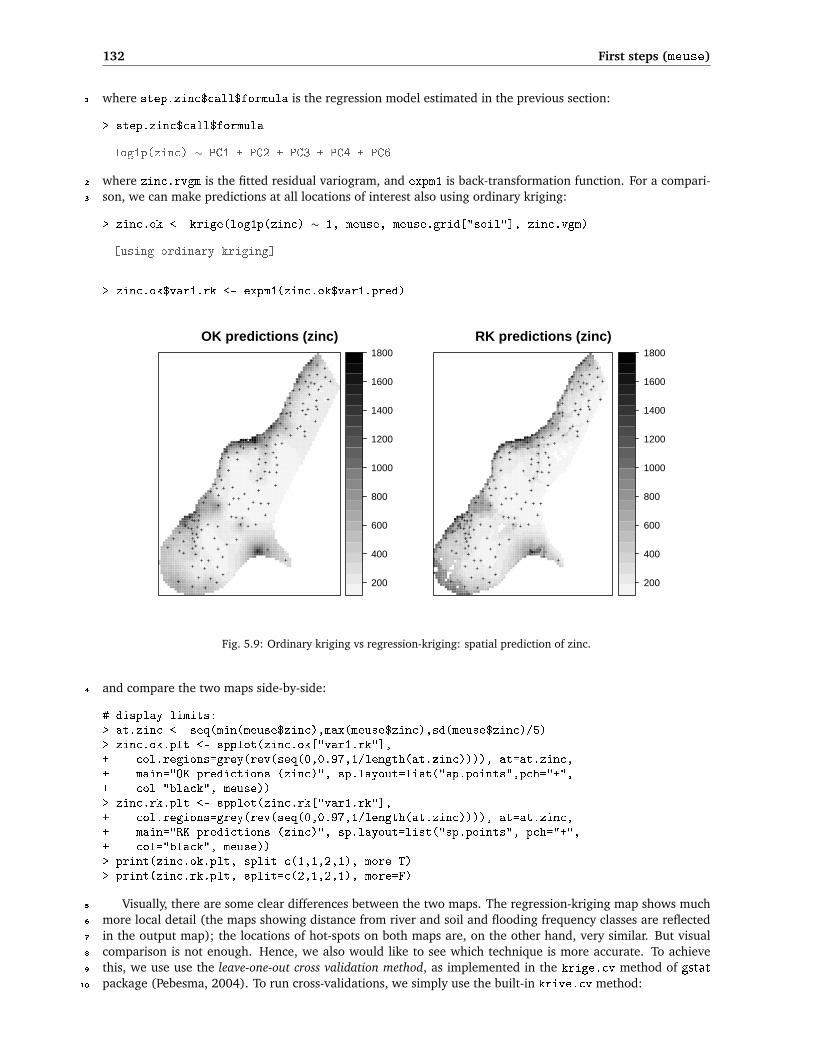
132 First steps (meuse)
where step.zinc$call$formula is the regression model estimated in the previous section:1
> step.zinc$call$formula
log1p(zinc) ∼ PC1 + PC2 + PC3 + PC4 + PC6
where zinc.rvgm is the fitted residual variogram, and expm1 is back-transformation function. For a compari-2
son, we can make predictions at all locations of interest also using ordinary kriging:3
> zinc.ok <- krige(log1p(zinc) ∼ 1, meuse, meuse.grid["soil"], zinc.vgm)
[using ordinary kriging]
> zinc.ok$var1.rk <- expm1(zinc.ok$var1.pred)
OK predictions (zinc)
++ + +
++
+++
+++
+++
++
++
+ +++
++++
++
+
+++ +
+++
+++
+++
+
+++
+
+++
++++++
++
++
++
++
++
++
+++
+ ++++
++
++
+
+
+
++
++
+
+ ++
+
++
+
+++
++
+
+
+
++
+
+
+++
++
+++
+
+
++
++
+
+
+
++
+
+
+
+
+
+
+
++
+
+++
+ ++
++
+++
+
++
+++
+
200
400
600
800
1000
1200
1400
1600
1800
RK predictions (zinc)
++ + +
++
+++
+++
+++
++
++
+ +++
++++
++
+
+++ +
+++
+++
+++
+
+++
+
+++
++++++
++
++
++
++
++
++
+++
+ ++++
++
++
+
+
+
++
++
+
+ ++
+
++
+
+++
++
+
+
+
++
+
+
+++
++
+++
+
+
++
++
+
+
+
++
+
+
+
+
+
+
+
++
+
+++
+ ++
++
+++
+
++
+++
+
200
400
600
800
1000
1200
1400
1600
1800
Fig. 5.9: Ordinary kriging vs regression-kriging: spatial prediction of zinc.
and compare the two maps side-by-side:4
# display limits:> at.zinc <- seq(min(meuse$zinc),max(meuse$zinc),sd(meuse$zinc)/5)> zinc.ok.plt <- spplot(zinc.ok["var1.rk"],+ col.regions=grey(rev(seq(0,0.97,1/length(at.zinc)))), at=at.zinc,+ main="OK predictions (zinc)", sp.layout=list("sp.points",pch="+",+ col="black", meuse))> zinc.rk.plt <- spplot(zinc.rk["var1.rk"],+ col.regions=grey(rev(seq(0,0.97,1/length(at.zinc)))), at=at.zinc,+ main="RK predictions (zinc)", sp.layout=list("sp.points", pch="+",+ col="black", meuse))> print(zinc.ok.plt, split=c(1,1,2,1), more=T)> print(zinc.rk.plt, split=c(2,1,2,1), more=F)
Visually, there are some clear differences between the two maps. The regression-kriging map shows much5
more local detail (the maps showing distance from river and soil and flooding frequency classes are reflected6
in the output map); the locations of hot-spots on both maps are, on the other hand, very similar. But visual7
comparison is not enough. Hence, we also would like to see which technique is more accurate. To achieve8
this, we use use the leave-one-out cross validation method, as implemented in the krige.cv method of gstat9
package (Pebesma, 2004). To run cross-validations, we simply use the built-in krive.cv method:10

5.4 Liming requirements 133
> cross.zinc.ok <- krige.cv(log1p(zinc) ∼ 1, meuse.ov,+ zinc.vgm, verbose=FALSE) # show no output> cross.zinc.rk <- krige.cv(step.zinc$call$formula, meuse.ov,+ zinc.rvgm, verbose=FALSE)
You will notice that the kriging system is solved once for each input data point. To evaluate the cross- 1
validation, we can compare RMSE summaries (§1.4), and in particular the standard deviations of the errors 2
(field residual of the cross-validation object). To estimate how much of variation has been explained by the 3
two models, we can run: 4
# amount of variation explained by the models:> 1-var(cross.zinc.ok$residual, na.rm=T)/var(log1p(meuse$zinc))
[1] 0.701
> 1-var(cross.zinc.rk$residual, na.rm=T)/var(log1p(meuse$zinc))
[1] 0.773
which shows that OK is not much worse than RK — RK is a better predictor, but the difference is only 7%. This 5
is possibly because variables dist and soil are also spatially continuous, and because the samples are equally 6
spread in geographic space. Indeed, if you look at Fig. 5.9 again, you will notice that the two maps do not 7
differ much. Note also that amount of variation explained by RK geostatistical model is about 80%, which is 8
satisfactory. 9
5.4 Liming requirements 10
5.4.1 Fitting a GLM 11
In the second part of this exercise, we will try to interpolate a categorical variable using the same regression- 12
kriging model. This variable is not as simple as zinc, since it ranges from 0 to 1 i.e. it is a binomial variable. 13
We need to respect that property of the data, and try to fit it using a GLM (Kutner et al., 2004): 14
E(Pc) = µ= g−1(q · β) (5.4.1)
15
where E(P) is the expected probability of class c (Pc ∈ [0,1]), q ·β is the linear regression model, and g is the 16
link function. Because the target variable is a binomial variable, we need to use the logit link function: 17
g(µ) = µ+ = ln�
µ
1−µ
�
(5.4.2)
18
so the Eq.(5.4.1) becomes logistic regression (Kutner et al., 2004). How does this works in R? Instead of fitting 19
a simple linear model (lm), we can use a more generic glm method with the logit link function (Fig. 5.10, 20
left): 21
> glm.lime <- glm(lime ∼ PC1+PC2+PC3+PC4+PC5+PC6+PC7+PC8, meuse.ov,+ family=binomial(link="logit"))> step.lime <- step(glm.lime)# check if the predictions are within 0-1 range:> summary(round(step.lime$fitted.values, 2))
Min. 1st Qu. Median Mean 3rd Qu. Max.0.000 0.010 0.090 0.284 0.555 0.920
What you do not see from your R session is that the GLM model is fitted iteratively, i.e. using a more 22
sophisticated approach than if we would simply fit a lm (e.g. using ordinary least square — no iterations). To 23
learn more about the GLMs and how are they fitted and how to interpret the results see Kutner et al. (2004). 24
Next, we can predict the values17 at all grid nodes using this model: 25
17Important: note that we focus on values in the transformed scale, i.e. logits.

134 First steps (meuse)
> p.glm <- predict(glm.lime, newdata=pc.comps, type="link", se.fit=T)> str(p.glm)
List of 3$ fit : Named num [1:3024] 2.85 2.30 2.25 1.83 2.77 .....- attr(*, "names")= chr [1:3024] "68" "144" "145" "146" ...$ se.fit : Named num [1:3024] 1.071 0.813 0.834 0.729 1.028 .....- attr(*, "names")= chr [1:3024] "68" "144" "145" "146" ...$ residual.scale: num 1
which shows that the spatial structure of the object was lost. Obviously, we will not be able to display the1
results as a map until we convert it to a gridded data frame. This takes few steps:2
# convert to a gridded layer:> lime.glm <- as(pc.comps, "SpatialPointsDataFrame")> lime.glm$lime <- p.glm$fit> gridded(lime.glm) <- TRUE> lime.glm <- as(lime.glm, "SpatialGridDataFrame")> proj4string(lime.glm) <- meuse.grid@proj4string
5.4.2 Variogram fitting and final predictions3
The remaining residuals we can interpolate using ordinary kriging. This is assuming that the residuals follow4
an approximately normal distribution. If the GLM we use is appropriate, this should indeed be the case. First,5
we estimate the variogram model:6
> hist(residuals(step.lime), breaks=25, col="grey")# residuals are normal;> lime.ivgm <- vgm(nugget=0, model="Exp",+ range=sqrt(diff(meuse@bbox["x",])^2 + diff(meuse@bbox["y", ])^2)/4,+ psill=var(residuals(step.lime)))> lime.rvgm <- fit.variogram(variogram(residuals(step.lime) ∼ 1, meuse.ov),+ model=lime.ivgm)
GLM fit (logits)
predicted (logits)
mea
sure
d
0.0
0.2
0.4
0.6
0.8
1.0
−10 −5 0
●●●
●●● ● ●●●● ●
●
●●
●●●●●●●●
●● ● ●● ●●● ●●● ● ● ●
● ●●
●● ●● ●●●●●●●
●●●●●
●●
●● ●●● ●●●
●
●
●
●●
●●
●
●●●
●● ● ●● ●
●
●
●●●●●
● ●
●●● ● ● ●●● ●●● ●● ●● ●●● ● ●●● ●●
●
●●● ●
●
● ●●●●● ● ●
●
●●● ● ● ● ● ●●● ● ●●● ●● ●●●●● ●● ●
Variogram for residuals
distance
sem
ivar
ianc
e
0.2
0.4
0.6
500 1000 1500
+
+
+ ++
+
++
+
+
+
+
+
+
+
57
299
419457547
533574
564589
543500
477
452457
415
Fig. 5.10: Measured and predicted (GLM with binomial function) values for lime variable (left); variogram for the GLMresiduals (right).
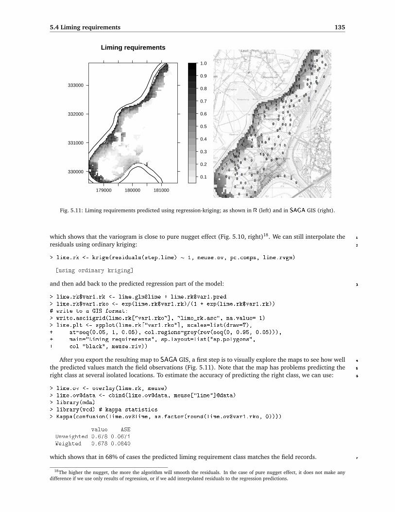
5.4 Liming requirements 135
Liming requirements
330000
331000
332000
333000
179000 180000 181000
0.1
0.2
0.3
0.4
0.5
0.6
0.7
0.8
0.9
1.0
Fig. 5.11: Liming requirements predicted using regression-kriging; as shown in R (left) and in SAGA GIS (right).
which shows that the variogram is close to pure nugget effect (Fig. 5.10, right)18. We can still interpolate the 1
residuals using ordinary kriging: 2
> lime.rk <- krige(residuals(step.lime) ∼ 1, meuse.ov, pc.comps, lime.rvgm)
[using ordinary kriging]
and then add back to the predicted regression part of the model: 3
> lime.rk$var1.rk <- lime.glm$lime + lime.rk$var1.pred> lime.rk$var1.rko <- exp(lime.rk$var1.rk)/(1 + exp(lime.rk$var1.rk))# write to a GIS format:> write.asciigrid(lime.rk["var1.rko"], "lime_rk.asc", na.value=-1)> lime.plt <- spplot(lime.rk["var1.rko"], scales=list(draw=T),+ at=seq(0.05, 1, 0.05), col.regions=grey(rev(seq(0, 0.95, 0.05))),+ main="Liming requirements", sp.layout=list("sp.polygons",+ col="black", meuse.riv))
After you export the resulting map to SAGA GIS, a first step is to visually explore the maps to see how well 4
the predicted values match the field observations (Fig. 5.11). Note that the map has problems predicting the 5
right class at several isolated locations. To estimate the accuracy of predicting the right class, we can use: 6
> lime.ov <- overlay(lime.rk, meuse)> lime.ov@data <- cbind(lime.ov@data, meuse["lime"]@data)> library(mda)> library(vcd) # kappa statistics> Kappa(confusion(lime.ov$lime, as.factor(round(lime.ov$var1.rko, 0))))
value ASEUnweighted 0.678 0.0671Weighted 0.678 0.0840
which shows that in 68% of cases the predicted liming requirement class matches the field records. 7
18The higher the nugget, the more the algorithm will smooth the residuals. In the case of pure nugget effect, it does not make anydifference if we use only results of regression, or if we add interpolated residuals to the regression predictions.

136 First steps (meuse)
5.5 Advanced exercises1
5.5.1 Geostatistical simulations2
A problem with kriging is that it over-smooths reality; especially processes that exhibits a nugget effect in the3
variogram model. The kriging predictor is the “best linear unbiased predictor” (BLUP) at each point, but the4
resulting field is commonly smoother than in reality (recall Fig. 1.4). This causes problems when running5
distributed models, e.g. erosion and runoff, and also gives a distorted view of nature to the decision-maker.6
A more realistic visualization of reality is achieved by the use of conditional geostatistical simulations:7
the sample points are taken as known, but the interpolated points reproduce the variogram model including8
the local noise introduced by the nugget effect. The same krige method in gstat can be used to generate9
simulations, by specifying the optional nsim (“number of simulations”) argument. It’s interesting to create10
several ‘alternate realities’, each of which is equally-probable. We can re-set R’s random number generator11
with the set.seed method to ensure that the simulations will be generated with the same random number12
seed19, and then generate four realizations:13
> set.seed(25)> zinc.rksim <- krige(step.zinc$call$formula, meuse.ov, pc.comps,+ zinc.rvgm, nsim=4, nmax=100)
drawing 4 GLS realisations of beta...[using conditional Gaussian simulation]
Now back-transform the predicted values, and plot all four simulations together:14
# back-transform the values:> for(i in 1:length(zinc.rksim@data)){> zinc.rksim@data[,i] <- expm1(zinc.rksim@data[,i])> }> spplot(zinc.rksim, col.regions=grey(c(rev(seq(0,0.97,1/length(at.zinc))),0)),+ at=at.zinc, main="RK simulations of log(zinc)")
RK simulations of log(zinc)
sim1 sim2 sim3 sim4
200
400
600
800
1000
1200
1400
1600
1800
Fig. 5.12: Four simulations of zinc using the fitted regression kriging model. Back-transformed to original scale (ppm).Compare with Fig. 5.9.
which shows that the general pattern of the zinc distribution repeats in each simulation (Fig. 5.12). However,15
we can also notice that some small features are not as clear as they look in Fig. 5.9. For example, it is16
relatively hard to notice the borders of the soil units, which in this case change from simulation to simulation.17
This confirms that the best predictor of zinc is the distance to the river (dist.asc map).18
To produce simulations of liming requirements, we can run (Bivand et al., 2008, p.230):19
19Hence differences between the simulated realizations are due only to the different values of the model parameters.

5.5 Advanced exercises 137
OK simulations of lime
sim1 sim2 sim3 sim4
0.0
0.2
0.4
0.6
0.8
1.0
Fig. 5.13: Four simulations of liming requirements (indicator variable) using ordinary kriging. Compare with Fig. 5.11.
# fit a variogram:> lime.ovgm <- fit.variogram(variogram(I(lime == 1) ∼ 1, meuse), vgm(1, "Sph", 800, 1))> lime.sim <- krige(I(lime == 1) ∼ 1, meuse, meuse.grid, lime.ovgm,+ nsim=4, indicators=TRUE, nmax=40)
drawing 4 GLS realisations of beta...[using conditional indicator simulation]
> spplot(lime.sim, col.regions=grey(c(rev(seq(0,0.9,0.05)), 0))+ main="OK simulations of lime")
the result is shown in Fig. 5.13. Note that in the case of liming requirements, there is a distinct difference 1
between the variogram of the original variable and of the residuals: most of spatially-correlated variation in 2
the lime requirements can be explained with auxiliary predictors, so that the variogram of residuals shows 3
pure nugget effect (Fig. 5.10, right). 4
5.5.2 Spatial prediction using SAGA GIS 5
Although SAGA has relatively limited geostatistical functionality, it contains a number of modules that are 6
of interest for geostatistical mapping: multiple linear regression (points and grids), ordinary kriging, and 7
regression-kriging. To start, we can examine if the algorithms implemented in gstat and SAGA are the same. 8
We can use the same model parameters estimated in section 5.3 to produce predictions of log1p(zinc). First, 9
we need to prepare vector and gridded maps in SAGA format: 10
# export the point data (transformed!):> meuse.ov$log1p_zinc <- log1p(meuse.ov$zinc)> writeOGR(meuse.ov["log1p_zinc"], ".", "zinc", "ESRI Shapefile")# export the grids to SAGA format:> PCs.list <- names(step.zinc$model)[-1]> for(i in PCs.list){> write.asciigrid(pc.comps[i], paste(i, ".asc", sep=""), na.value=-9999)> }> rsaga.esri.to.sgrd(in.grids=set.file.extension(PCs.list, ".asc"),+ out.sgrds=set.file.extension(PCs.list, ".sgrd"), in.path=getwd())
and then make the predictions by using the Universal kriging module in SAGA (Fig. 5.14): 11
# regression-kriging using the same parameters fitted previously:> gridcell <- pc.comps@grid@cellsize[1]

138 First steps (meuse)
> rsaga.geoprocessor(lib="geostatistics_kriging", module=8,+ param=list(GRID="zinc_rk_SAGA.sgrd", SHAPES="zinc.shp",+ GRIDS=paste(set.file.extension(PCs.list, ".sgrd"), collapse=";", sep=""),+ BVARIANCE=F, BLOCK=F, FIELD=1, BLOG=F, MODEL=1, TARGET=0,+ USER_CELL_SIZE=gridcell, NUGGET=zinc.rvgm$psill[1], SILL=zinc.rvgm$psill[2],+ RANGE=zinc.rvgm$range[2], INTERPOL=0,+ USER_X_EXTENT_MIN=pc.comps@bbox[1,1]+gridcell/2,+ USER_X_EXTENT_MAX=pc.comps@bbox[1,2]-gridcell/2,+ USER_Y_EXTENT_MIN=pc.comps@bbox[2,1]+gridcell/2,+ USER_Y_EXTENT_MAX=pc.comps@bbox[2,2]-gridcell/2))
SAGA CMD 2.0.4library path: C:/Progra∼1/saga_vc/moduleslibrary name: geostatistics_krigingmodule name : Universal Kriging (Global)author : (c) 2003 by O.Conrad
Load shapes: zinc.shp...ready
Load grid: PC1.sgrd...ready
...
Load grid: PC6.sgrd...ready
Parameters
Grid: [not set]Variance: [not set]Points: zinc.shpAttribute: log1p_zincCreate Variance Grid: noTarget Grid: user definedVariogram Model: Exponential ModelBlock Kriging: noBlock Size: 100.000000Logarithmic Transformation: noNugget: 0.054588Sill: 0.150518Range: 374.198454Linear Regression: 1.000000Exponential Regression: 0.100000Power Function - A: 1.000000Power Function - B: 0.500000Grids: 5 objects (PC1.sgrd, PC2.sgrd, PC3.sgrd, PC4.sgrd, PC6.sgrd))Grid Interpolation: Nearest Neighbor
Save grid: zinc_rk_SAGA.sgrd...
Visually (Fig. 5.14), the results look as if there is no difference between the two pieces of software. We can1
then load back the predictions into R to compare if the results obtained with gstat and SAGA match exactly:2
> rsaga.sgrd.to.esri(in.sgrds="zinc_rk_SAGA",+ out.grids="zinc_rk_SAGA.asc", out.path=getwd())> zinc.rk$SAGA <- readGDAL("zinc_rk_SAGA.asc")$band1> plot(zinc.rk$SAGA, zinc.rk$var1.pred, pch=19, xlab="SAGA", ylab="gstat")> lines(3:8, 3:8, col="grey", lwd=4)

5.5 Advanced exercises 139
which shows that both software programs implement the same algorithm, but there are some small differences 1
between the predicted values that are possibly due to rounding effect. 2
Fig. 5.14: Comparing results from SAGA (left map) and gstat (right map): regression-kriging using the same modelparameters estimated in section 5.3.
Next, we want to compare the computational efficiency of gstat and SAGA, i.e. the processing time. To 3
emphasize the difference in computation time, we will use a somewhat larger grid (2 m), and then re-run 4
ordinary kriging in both software packages: 5
> meuse.grid2m <- readGDAL("topomap2m.tif")
topomap2m.tif has GDAL driver GTiffand has 1664 rows and 1248 columns
> proj4string(meuse.grid2m) <- meuse.grid@proj4string
Processing speed can be measured from R by using the system.time method, which measures the elapsed 6
seconds: 7
> system.time(krige(log1p(zinc) ∼ 1, meuse, meuse.grid2m, zinc.vgm))
[using ordinary kriging]user system elapsed
319.14 7.96 353.44
and now the same operation in SAGA: 8
> cellsize2 <- meuse.grid2m@grid@cellsize[1]> system.time(rsaga.geoprocessor(lib="geostatistics_kriging", module=6,+ param=list(GRID="zinc_ok_SAGA.sgrd", SHAPES="zinc.shp", BVARIANCE=F, BLOCK=F,+ FIELD=1, BLOG=F, MODEL=1, TARGET=0, USER_CELL_SIZE=cellsize2,+ NUGGET=zinc.vgm$psill[1], SILL=zinc.vgm$psill[2], RANGE=zinc.rvgm$range[2],+ USER_X_EXTENT_MIN=meuse.grid2m@bbox[1,1]+cellsize2/2,+ USER_X_EXTENT_MAX=meuse.grid2m@bbox[1,2]-cellsize2/2,+ USER_Y_EXTENT_MIN=meuse.grid2m@bbox[2,1]+cellsize2/2,+ USER_Y_EXTENT_MAX=meuse.grid2m@bbox[2,2]-cellsize2/2)))
user system elapsed0.03 0.71 125.69

140 First steps (meuse)
We can see that SAGA will be faster for processing large data sets. This difference will become even larger1
if we would use large point data sets. Recall that the most ‘expensive’ operation for any geostatistical mapping2
is the derivation of distances between points. Thus, by limiting the search radius one can always increase3
the processing speed. The problem is that a software needs to initially estimate which points fall within the4
search radius, hence it always has to take into account location of all points. Various quadtree and similar5
algorithms then exist to speed up the neighborhood search algorithm (partially available in gstat also), but6
their implementation can differ between various programming languages.7
Note also that it is not really a smart idea to try to visualize large maps in R. R graphics plots grids as8
vectors; each grid cell is plotted as a separate polygon, which takes a huge amount of RAM for large grids,9
and can last up to few minutes. SAGA on other hand can handle and display grids �10 million pixels on a10
standard PC without any delays (Fig. 5.14). When you move to other exercises you will notice that we will11
typically use R to fit models, SAGA to run predictions and visualize results, and Google Earth to visualize and12
explore final products.13
5.5.3 Geostatistical analysis in geoR14
We start by testing the variogram fitting functionality of geoR. However, before we can do any analysis, we15
need to convert our point map (sp) to geoR geodata format:16
> zinc.geo <- as.geodata(meuse.ov["zinc"])> str(zinc.geo)
List of 2$ x , y : num [1:155, 1:2] 181072 181025 181165 181298 181307 .....- attr(*, "dimnames")=List of 2.. ..$ : chr [1:155] "300" "455" "459" "540" ..... ..$ : chr [1:2] "x" "y"$ data : num [1:155] 1022 1141 640 257 269 ...- attr(*, "class")= chr "geodata"
0 500 1000
0.0
0.2
0.4
0.6
0.8
1.0
distance
sem
ivar
ianc
e
0°°45°°90°°135°°
●●
●
●
●
●
●
● ●●
●●
●
0 500 1000
0.0
0.2
0.4
0.6
0.8
1.0
1.2
1.4
distance
sem
ivar
ianc
e
Fitted variogram (ML)
Fig. 5.15: Anisotropy (left) and variogram model fitted using the Maximum Likelihood (ML) method (right). The con-fidence bands (envelopes) show the variability of the sample variogram estimated using simulations from a given set ofmodel parameters.

5.5 Advanced exercises 141
which shows much simpler structure than a SpatialPointsDataFrame. A geodata-type object contains only: 1
a matrix with coordinates of sampling locations (coords), values of target variables (data), matrix with coor- 2
dinates of the polygon defining the mask map (borders), vector or data frame with covariates (covariate). 3
To produce the two standard variogram plots (Fig. 5.15), we will run: 4
> par(mfrow=c(1,2))# anisotropy ("lambda=0" indicates log-transformation):> plot(variog4(zinc.geo, lambda=0, max.dist=1500, messages=FALSE), lwd=2)# fit variogram using likfit:> zinc.svar2 <- variog(zinc.geo, lambda=0, max.dist=1500, messages=FALSE)> zinc.vgm2 <- likfit(zinc.geo, lambda=0, messages=FALSE,+ ini=c(var(log1p(zinc.geo$data)),500), cov.model="exponential")> zinc.vgm2
likfit: estimated model parameters:beta tausq sigmasq phi
" 6.1553" " 0.0164" " 0.5928" "500.0001"Practical Range with cor=0.05 for asymptotic range: 1498
likfit: maximised log-likelihood = -1014
# generate confidence bands for the variogram:> env.model <- variog.model.env(zinc.geo, obj.var=zinc.svar2, model=zinc.vgm2)
variog.env: generating 99 simulations (with 155 points each) using grfvariog.env: adding the mean or trendvariog.env: computing the empirical variogram for the 99 simulationsvariog.env: computing the envelops
> plot(zinc.svar2, envelope=env.model); lines(zinc.vgm2, lwd=2);> legend("topleft", legend=c("Fitted variogram (ML)"), lty=c(1), lwd=c(2), cex=0.7)> dev.off()
where variog4 is a method that generates semivariances in four directions, lambda=0 is used to indicate the 5
type of transformation20, likfit is the generic variogram fitting method, ini is the given initial variogram, 6
and variog.model.env calculates confidence limits for the fitted variogram model. Parameters tausq and 7
sigmasq corresponds to nugget and sill parameters; phi is the range parameter. 8
In general, geoR offers much richer possibilities for variogram modeling than gstat. From Fig. 5.15(right) 9
we can see that the variogram fitted using this method does not really go through all points (compare with 10
Fig. 5.8). This is because the ML method discounts the potentially wayward influence of sample variogram at 11
large inter-point distances (Diggle and Ribeiro Jr, 2007). Note also that the confidence bands (envelopes) also 12
confirm that the variability of the empirical variogram increases with larger distances. 13
Now that we have fitted the variogram model, we can produce predictions using the ordinary kriging 14
model. Because geoR does not work with sp objects, we need to prepare the prediction locations: 15
> locs <- pred_grid(c(pc.comps@bbox[1,1]+gridcell/2,+ pc.comps@bbox[1,2]-gridcell/2), c(pc.comps@bbox[2,1]+gridcell/2,+ pc.comps@bbox[2,2]-gridcell/2), by=gridcell)# match the same grid as pc.comps;
and the mask map i.e. a polygon showing the borders of the area of interest: 16
> meuse.grid$mask <- ifelse(!is.na(meuse.grid$dist), 1, NA)> write.asciigrid(meuse.grid["mask"], "mask.asc", na.value=-1)# raster to polygon conversion;> rsaga.esri.to.sgrd(in.grids="mask.asc", out.sgrd="mask.sgrd", in.path=getwd())> rsaga.geoprocessor(lib="shapes_grid", module=6, param=list(GRID="mask.sgrd",
20geoR implements the Box–Cox transformation (Diggle and Ribeiro Jr, 2007, p.61), which is somewhat more generic than simplelog() transformation.

142 First steps (meuse)
+ SHAPES="mask.shp", CLASS_ALL=1))> mask <- readShapePoly("mask.shp", proj4string=CRS("+init=epsg:28992"),+ force_ring=T)# coordinates of polygon defining the area of interest:> mask.bor <- mask@polygons[[1]]@Polygons[[1]]@coords> str(mask.bor)
num [1:267, 1:2] 178880 178880 178760 178760 178720 ...
Ordinary kriging can be run by using the generic method for linear Gaussian models krige.conv21:1
> zinc.ok2 <- krige.conv(zinc.geo, locations=locs,+ krige=krige.control(obj.m=zinc.vgm2), borders=mask.bor)
krige.conv: results will be returned only for locations inside the borderskrige.conv: model with constant meankrige.conv: performing the Box-Cox data transformationkrige.conv: back-transforming the predicted mean and variancekrige.conv: Kriging performed using global neighborhood
# Note: geoR will automatically back-transform the values!> str(zinc.ok2)
List of 6$ predict : num [1:3296] 789 773 756 740 727 ...$ krige.var : num [1:3296] 219877 197718 176588 159553 148751 ...$ beta.est : Named num 6.16..- attr(*, "names")= chr "beta"$ distribution: chr "normal"$ message : chr "krige.conv: Kriging performed using global neighbourhood"$ call : language krige.conv(geodata = zinc.geo, locations = locs,
borders = mask.bor, krige = krige.control(obj.m = zinc.vgm2))- attr(*, "sp.dim")= chr "2d"- attr(*, "prediction.locations")= symbol locs- attr(*, "parent.env")=<environment: R_GlobalEnv>- attr(*, "data.locations")= language zinc.geo$coords- attr(*, "borders")= symbol mask.bor- attr(*, "class")= chr "kriging"
To produce plots shown in Fig. 5.16, we use:2
> par(mfrow=c(1,2))> image(zinc.ok2, loc=locs, col=gray(seq(1,0.1,l=30)), xlab="Coord X",+ ylab="Coord Y")> title(main="Ordinary kriging predictions")> contour(zinc.ok2, add=TRUE, nlev=8)> image(zinc.ok2, loc=locs, value=sqrt(zinc.ok2$krige.var),+ col=gray(seq(1,0.1,l=30)), xlab="Coord X", ylab="Coord Y")> title(main="Prediction error")> krige.var.vals <- round(c(quantile(sqrt(zinc.ok2$krige.var),0.05),+ sd(zinc.geo$data), quantile(sqrt(zinc.ok2$krige.var), 0.99)), 0)> legend.krige(x.leg=c(178500,178800), y.leg=c(332500,333500),+ values=sqrt(zinc.ok2$krige.var), vert=TRUE, col=gray(seq(1,0.1,l=30)),+ scale.vals=krige.var.vals)> points(zinc.geo[[1]], pch="+", cex=.7)
To run regression-kriging (in geoR “external trend kriging”) we first need to add values of covariates to the3
original geodata object:4
21Meaning “kriging conventional” i.e. linear kriging.

5.5 Advanced exercises 143
Fig. 5.16: Zinc predicted using ordinary kriging in geoR. The map on the left is considered to be below critical accuracylevel in the areas where the prediction error (right map) exceeds the global variance (the middle value in legend). Comparewith Fig. 5.9.
> zinc.geo$covariate <- meuse.ov@data[,PCs.list]
which now allows us to incorporate the trend argument in the variogram model: 1
# trend model:> step.zinc$call$formula[c(1,3)]
∼ PC1 + PC2 + PC3 + PC4 + PC6
> zinc.rvgm2 <- likfit(zinc.geo, lambda=0, trend=step.zinc$call$formula[c(1,3)],+ messages=FALSE, ini=c(var(residuals(step.zinc)),500), cov.model="exponential")> zinc.rvgm2
likfit: estimated model parameters:beta0 beta1 beta2 beta3 beta4 beta5
" 5.6919" " -0.4028" " -0.1203" " -0.0176" " 0.0090" " -0.3199"tausq sigmasq phi
" 0.0526" " 0.1894" "499.9983"Practical Range with cor=0.05 for asymptotic range: 1498
likfit: maximised log-likelihood = -975
Note that geoR reports also the regression coefficients for the five predictors (beta0 is the intercept). In 2
the case of gstat this information will be hidden: gstat will typically fit a regression model only to derive the 3
residuals (regression coefficients can be printed by setting the debugging options). Neither gstat nor geoR 4
report on the goodness of fit and similar regression diagnostics. 5
Before we can make predictions, we also need to prepare the covariates at all locations. Unfortunately, 6
geoR is not compatible with sp grids, so we need to prepare the covariate values so they exactly match 7
prediction locations: 8
# get values of covariates at new locations:> locs.sp <- locs> coordinates(locs.sp) <- ∼ Var1+Var2

144 First steps (meuse)
> PCs.gr <- overlay(pc.comps, locs.sp)# fix NAs:> for(i in PCs.list){> PCs.gr@data[,i] <- ifelse(is.na(PCs.gr@data[,i]), 0, PCs.gr@data[,i])> }
which allows us to run predictions using the same trend model as used in section 5.3.1:1
# define the geostatistical model:> KC <- krige.control(trend.d = step.zinc$call$formula[c(1,3)],+ trend.l = ∼ PCs.gr$PC1+PCs.gr$PC2+PCs.gr$PC3+PCs.gr$PC4+PCs.gr$PC6,+ obj.m = zinc.rvgm2)# run predictions (external trend kriging):> zinc.rk2 <- krige.conv(zinc.geo, locations=locs, krige=KC, borders=mask.bor)
krige.conv: results will be returned only for prediction inside the borderskrige.conv: model with mean defined by covariates provided by the userkrige.conv: performing the Box-Cox data transformationkrige.conv: back-transforming the predicted mean and variancekrige.conv: Kriging performed using global neighbourhood
Fig. 5.17: Zinc predicted using external trend kriging in geoR (left); simulations using the same model (right). Comparewith Figs. 5.9 and 5.12.
The result is shown in Fig. 5.17. geoR also allows generation of simulations using the same external trend2
model by setting the output.control parameter (the resulting map shown in Fig. 5.17; right):3
> zinc.rk2 <- krige.conv(zinc.geo, locations=locs, krige=KC, borders=mask.bor,+ output=output.control(n.predictive=1))
krige.conv: results will be returned only for prediction inside the borderskrige.conv: model with mean defined by covariates provided by the userkrige.conv: performing the Box-Cox data transformationkrige.conv: sampling from the predictive distribution (conditional simulations)krige.conv: back-transforming the simulated valueskrige.conv: back-transforming the predicted mean and variancekrige.conv: Kriging performed using global neighborhood

5.6 Visualization of generated maps 145
which shows a somewhat higher range of values than the simulation using a simple linear model (Fig. 5.12). In 1
this case geoR seems to do better in accounting for the skewed distribution of values than gstat. However such 2
simulations in geoR are extremely computationally intensive, and are not recommended for large data sets. 3
In fact, many default methods implemented in geoR (Maximum Likelihood fitting for variograms, Bayesian 4
methods and conditional simulations) are definitively not recommended with data sets with�1000 sampling 5
points and/or over �100,000 new locations. Creators of geoR seem to have selected a path of running only 6
global neighborhood analysis on the point data. Although the author of this guide supports that decision (see 7
also section 2.2), some solution needs to be found to process larger point data sets because computing time 8
exponentially increases with the size of the data set. 9
Finally, the results of predictions can be exported22 to some GIS format by copying the values to an sp 10
frame: 11
> mask.ov <- overlay(mask, locs.sp)> mask.sel <- !is.na(mask.ov$MASK.SGRD)> locs.geo <- data.frame(X=locs.sp@coords[mask.sel,1],+ Y=locs.sp@coords[mask.sel,2], zinc.rk2=zinc.rk2[[1]],+ zinc.rkvar2=zinc.rk2[[2]])> coordinates(locs.geo) <- ∼ X+Y> gridded(locs.geo) <- TRUE> write.asciigrid(locs.geo[1], "zinc_rk2.asc", na.value=-1)
5.6 Visualization of generated maps 12
5.6.1 Visualization of uncertainty 13
The following paragraphs explain how to visualize results of geostatistical mapping to explore uncertainty in 14
maps. We will focus on the technique called whitening, which is a simple but efficient technique to visualize 15
mapping error (Hengl and Toomanian, 2006). It is based on the Hue-Saturation-Intensity (HSI) color model 16
(Fig. 5.18a) and calculations with colors using the color mixture (CM) concept. The HSI is a psychologically 17
appealing color model — hue is used to visualize values or taxonomic space and whiteness (paleness) is used to 18
visualize the uncertainty (Dooley and Lavin, 2007). For this purpose, a 2D legend was designed to accompany 19
the visualizations. Unlike standard legends for continuous variables, this legend has two axis (Fig. 5.18b): 20
(1) vertical axis (hues) is used to visualize the predicted values and (2) horizontal axis (whiteness) is used to 21
visualize the prediction error. Fig. 5.19 shows an example of visualization using whitening for the meuse data 22
set. 23
Visualization of uncertainty in maps using whitening can be achieved using one of the two software pro- 24
grams: ILWIS and R. In ILWIS, you can use the VIS_error script that can be obtained from the author’s 25
homepage. To visualize the uncertainty for your own case study using this technique, you should follow these 26
steps (Hengl and Toomanian, 2006): 27
(1.) Download the ILWIS script (VIS_error23) for visualization of prediction error and unzip it to the default 28
directory (C:\Program Files\ILWIS\Scripts\). 29
(2.) Derive the predictions and prediction variance for some target variable. Import both maps to ILWIS. The 30
prediction variance needs to be then converted to normalized prediction variance by using Eq.(1.4.4), 31
so you will also need to determine the global variance of your target variable. 32
(3.) Start ILWIS and run the script from the left menu (operations list) or from the main menu 7→ Operations 33
7→ Scripts 7→ VIS_error. Use the help button to find more information about the algorithm. 34
(4.) To prepare final layouts, you will need to use the legend2D.tif legend file24. 35
A more interesting option is to visualize maps using whitening in R25. You will need to load the following 36
additional package: 37
22Note that the results of prediction in geoR is simply a list of values without any spatial reference.23http://spatial-analyst.net/scripts/24http://spatial-analyst.net/scripts/legend2D.tif; This legend is a Hue-whitening legend: in the vertical direction only
Hue values change, while in the horizontal direction amount of white color is linearly increased from 0.5 up to 1.0.25http://spatial-analyst.net/scripts/whitening.R

146 First steps (meuse)
> library(colorspace)
The example with the meuse data set:1
# ordinary kriging:> m <- vgm(.59, "Sph", 874, .04)> vismaps <- krige(log(zinc) ∼ 1, meuse, meuse.grid, model=m)
As a result of ordinary kriging, we have produced two maps: predictions and the prediction variance. Now,2
we can visualize both maps together using whitening. We start by setting up threshold levels (lower and upper3
limits), and stretching the values within that range:4
> z1 <- min(log(meuse$zinc), na.rm=TRUE)> z2 <- max(log(meuse$zinc), na.rm=TRUE)> e1 <- 0.4> e2 <- 0.7> vismaps$er <- sqrt(vismaps$e)/sqrt(var(log(meuse$zinc)))> vismaps$tmpz <- (vismaps$z-z1)/(z2-z1)# Mask the values outside the 0-1 range:> vismaps$tmpzc <- ifelse(vismaps$tmpz<=0, 0, ifelse(vismaps$tmpz>1, 1, vismaps$tmpz))
The Hue-Saturation-Value (HSV) bands we can generate using:5
# The hues should lie between between 0 and 360, and the saturations# and values should lie between 0 and 1.> vismaps$tmpf1 <- -90-vismaps$tmpzc*300> vismaps$tmpf2 <- ifelse(vismaps$tmpf1<=-360, vismaps$tmpf1+360, vismaps$tmpf1)> vismaps$H <- ifelse(vismaps$tmpf2>=0, vismaps$tmpf2, (vismaps$tmpf2+360))# Strech the error values (e) to the inspection range:# Mask the values out of the 0-1 range:> vismaps$tmpe <- (vismaps$er-e1)/(e2-e1)> vismaps$tmpec <- ifelse(vismaps$tmpe<=0, 0, ifelse(vismaps$tmpe>1, 1, vismaps$tmpe))# Derive the saturation and intensity images:> vismaps$S <- 1-vismaps$tmpec> vismaps$V <- 0.5*(1+vismaps$tmpec)
The HSV values can be converted to RGB bands using:6
> RGBimg <- as(HSV(vismaps$H, vismaps$S, vismaps$V), "RGB")> summary(RGBimg@coords)> vismaps$red <- as.integer(ifelse(is.na(vismaps@data[1]), 255, RGBimg@coords[,1]*255))> vismaps$green <- as.integer(ifelse(is.na(vismaps@data[1]), 255, RGBimg@coords[,2]*255))> vismaps$blue <- as.integer(ifelse(is.na(vismaps@data[1]), 255, RGBimg@coords[,3]*255))> summary(vismaps[c("red", "green", "blue")])
Object of class SpatialGridDataFrameCoordinates:
min maxx 178440 181560y 329600 333760Is projected: NAproj4string : [NA]Number of points: 2Grid attributes:cellcentre.offset cellsize cells.dim
x 178460 40 78y 329620 40 104Data attributes:
red green blueMin. : 0.0 Min. : 0.0 Min. : 0.01st Qu.:153.0 1st Qu.:183.0 1st Qu.:194.0Median :255.0 Median :255.0 Median :255.0Mean :206.2 Mean :220.5 Mean :219.23rd Qu.:255.0 3rd Qu.:255.0 3rd Qu.:255.0Max. :255.0 Max. :255.0 Max. :255.0

5.6 Visualization of generated maps 147
Fig. 5.18: Design of the special 2D legend used to visualize the prediction variance using whitening: (a) the HSI colormodel, (b) the 2D legend and (c) the common types of Hues. After Hengl et al. (2004a).
178440 181560
178440 181560
333760
329600
178440 181560
178440 181560
333760
329640
333760
329640
ordinary kriging
4.72
7.51
40% 70%universal kriging
333760
329600
Fig. 5.19: Mapping uncertainty for zinc visualized using whitening: ordinary kriging (left) and universal kriging (right).Predicted values in log-scale. See cover of this book for a color version of this figure.

148 First steps (meuse)
which is now a spatial object with three RGB bands. To display a true RGB image in R, use the SGDF2PCT1
method26:2
> RGBimg <- SGDF2PCT(vismaps[c("red", "green", "blue")], ncolors=256, adjust.bands=FALSE)> vismaps$idx <- RGBimg$idx> image(vismaps, "idx", col=RGBimg$ct)> plot(meuse, pch="+", add=TRUE)
In the last step (optional), we can set the right georeference and export the map to e.g. GeoTIFF format:3
> proj4string(vismaps) <- CRS("+init=epsg:28992")# Export as geoTIFF / or any other format:> writeGDAL(vismaps[c("red", "green", "blue")], "vismap.tif", drivername="GTiff",+ type="Byte", options="INTERLEAVE=PIXEL")
A comparison of uncertainty for maps produced using ordinary kriging and universal kriging in gstat can4
be seen in Fig. 5.19. In this case, the universal kriging map is distinctly more precise. You can manually change5
the lower and upper values for both prediction and error maps depending on your mapping requirements. By6
default, thresholds of 0.4 and 0.8 (max 1.0) are used for the normalized prediction error values. This assumes7
that a satisfactory prediction is when the model explains more than 85% of the total variation (normalized8
error = 40%; see p.23). Otherwise, if the value of the normalized error get above 80%, the model accounts9
for less than 50% of variability at calibration points and the prediction is probably unsatisfactory.10
To prepare the 2D legend shown in Fig. 5.19 (100×100 pixels), we use:11
> legend.2D <- expand.grid(x=seq(.01,1,.01),y=seq(.01,1,.01))# Hues> legend.2D$tmpf1 <- -90-legend.2D$y*300> legend.2D$tmpf2 <- ifelse(legend.2D$tmpf1<=-360, legend.2D$tmpf1+360,+ legend.2D$tmpf1)> legend.2D$H <- ifelse(legend.2D$tmpf2>=0, legend.2D$tmpf2, (legend.2D$tmpf2+360))# Saturation:> legend.2D$S <- 1-legend.2D$x# Intensity:> legend.2D$V <- 0.5+legend.2D$x/2> gridded(legend.2D) <- ∼ x+y> legend.2D <- as(legend.2D, "SpatialGridDataFrame")> legendimg <- as(HSV(legend.2D$H, legend.2D$S, legend.2D$V), "RGB")> legend.2D$red <- as.integer(legendimg@coords[,1]*255)> legend.2D$green <- as.integer(legendimg@coords[,2]*255)> legend.2D$blue <- as.integer(legendimg@coords[,3]*255)# Write as a RGB image:> legend.2Dimg <- SGDF2PCT(legend.2D[c("red", "green", "blue")], ncolors=256,+ adjust.bands=FALSE)> legend.2D$idx <- legend.2Dimg$idx> writeGDAL(legend.2D[c("red", "green", "blue")], "legend2D.tif",+ drivername="GTiff", type="Byte", options="INTERLEAVE=PIXEL")
Another sophisticated option to visualize the results of (spatio-temporal) geostatistical mapping is the12
stand-alone visualization software called Aquila27 (Pebesma et al., 2007). Aquila facilitates interactive ex-13
ploration of the spatio-temporal Cumulative Distribution Functions (CDFs) and allows decision makers to14
explore uncertainty associated with attaching different threshold or its spatial distribution in the area of in-15
terest. It is actually rather simple to use — one only needs to prepare a sample (e.g. 12 slices) of quantile16
estimates, which are then locally interpolated to produce CDFs.17
5.6.2 Export of maps to Google Earth18
To export maps we have produced to Google Earth, we first need to reproject the maps to the WGS84 coordi-19
nate system (the native system for Google Earth). We can first reproject the map of sample points, using the20
26Note that the results might differ slightly between ILWIS and R, which is mainly due to somewhat different HSI–RGB conversionalgorithms. For example, the SGDF2PCT method is limited to 256 colors only!
27http://pcraster.geo.uu.nl/projects/aguila/

5.6 Visualization of generated maps 149
spTransform method of the sp package, and then export them using writeOGR: 1
> meuse.ll <- spTransform(meuse, CRS("+proj=longlat +datum=WGS84"))> writeOGR(meuse.ll, "meuse.kml", "meuse", driver="KML")
You can examine these in Google Earth by opening the KML file meuse.kml which you just wrote. Next, 2
we want to export the predictions of zinc, which means that we first need to reproject the interpolated values 3
onto geographic coordinates. The most efficient way to achieve this is by using the SAGA proj4 module28: 4
> rsaga.geoprocessor(lib="pj_proj4", 2, param=list(SOURCE_PROJ=paste('"',+ proj4string(meuse.grid), '"', sep=""), TARGET_PROJ="\"+proj=longlat+ +datum=WGS84\"", SOURCE="zinc_rk.sgrd", TARGET="zinc_rk_ll.sgrd",+ TARGET_TYPE=0, INTERPOLATION=1))
SAGA CMD 2.0.4library path: C:/Progra∼1/saga_vc/moduleslibrary name: pj_proj4module name : Proj.4 (Command Line Arguments, Grid)author : O. Conrad (c) 2004-8
Load grid: zinc_rk.sgrd...ready
Parameters
Inverse: noSource Projection Parameters: +init=epsg:28992 +proj=sterea+lat_0=52.15616055555555 +lon_0=5.38763888888889 +k=0.999908 +x_0=155000+y_0=463000 +ellps=bessel +towgs84=565.237,50.0087,465.658,-0.406857,0.350733,-1.87035,4.0812 +units=m +no_defsTarget Projection Parameters: +proj=longlat +datum=WGS84Grid system: 40; 77x 104y; 178500x 329620ySource: zinc_rk.sgrdTarget: [not set]Shapes: [not set]X Coordinates: [not set]Y Coordinates: [not set]Create X/Y Grids: noTarget: user definedInterpolation: Bilinear Interpolation
Source: +init=epsg:28992 +proj=sterea +lat_0=52.15616055555555+lon_0=5.38763888888889 +k=0.999908 +x_0=155000 +y_0=463000+ellps=bessel +towgs84=565.237,50.0087,465.658,-0.406857,0.350733,-1.87035,4.0812 +units=m +no_defs
Target: +proj=longlat +datum=WGS84
readySave grid: zinc_rk_ll.sgrd...
Once we have created this gridded result, we can plot the maps and export the plots to Google Earth. First 5
we need to set up metadata in the form of a SpatialGrid object for defining the size and placing of a PNG 6
image overlay in Google Earth; this is the job of the GE_SpatialGrid method of the maptools package: 7
# read back into R:> rsaga.sgrd.to.esri(in.sgrds="zinc_rk_ll.sgrd", out.grids="zinc_rk_ll.asc",+ out.path=getwd())> zinc_rk.ll <- readGDAL("zinc_rk_ll.asc")
28SAGA will automatically estimate both the grid cell size and the bounding box in geographical coordinates. Compare with sec-tion 10.6.3.

150 First steps (meuse)
zinc_rk_ll.asc has GDAL driver AAIGridand has 105 rows and 122 columns
> proj4string(zinc_rk.ll) <- CRS("+proj=longlat +datum=WGS84")> zinc_rk.kml <- GE_SpatialGrid(zinc_rk.ll)
Fig. 5.20: RK predictions of zinc for Meuse area — as visualized in Google Earth.
where zinc_rk.kml is the name of R object, which carries only a definition of the ground overlay frame and1
not the data to be exported. Next we create a PNG (Portable Network Graphics) file (the format recognized as2
an overlay by Google Earth) using the png graphics device:3
> png(file="zinc_rk.png", width=zinc_rk.kml$width, height=zinc_rk.kml$height, bg="transparent")> par(mar=c(0,0,0,0), xaxs="i", yaxs="i")> image(as.image.SpatialGridDataFrame(zinc_rk.ll[1]),+ col=grey(rev(seq(0,0.95,1/length(at.zinc)))),+ xlim=zinc_rk.kml$xlim, ylim=zinc_rk.kml$ylim)
which will plot the map over the whole area of the plotting space, so that border coordinates exactly match4
the borders of the plot. We then create the overlay itself, from the PNG file, with the kmlOverlay method,5
specifying the SpatialGrid object that orients the map in Google Earth:6
> kmlOverlay(zinc_rk.kml, kmlfile="zinc_rk.kml", imagefile="zinc_rk.png", name="zinc")
[1] "<?xml version='1.0' encoding='UTF-8'?>"[2] "<kml xmlns='http://earth.google.com/kml/2.0'>"[3] "<GroundOverlay>"

5.6 Visualization of generated maps 151
[4] "<name>zinc (RK)</name>"[5] "<Icon><href>zinc_rk.png</href><viewBoundScale>0.75</viewBoundScale></Icon>"[6] "<LatLonBox><north>50.992973</north><south>50.955488</south>+ <east>5.76502299201062</east><west>5.721466</west></LatLonBox>"[7] "</GroundOverlay></kml>"
> dev.off()
When you open the resulting KML in Google Earth, you will see a display shown in Fig. 5.20. This allows 1
you to orient yourself and make an interpretation of the produced maps. Open the final map in Google Earth 2
and visually explore how many areas next to the populated areas show high concentrations of zinc. 3
Self-study exercises: 4
(1.) How many pixels in the meuse.grid are available for spatial prediction? (HINT: Number of pixels that 5
do not have missing values for any of the variables.) 6
(2.) What is the correlation coefficient between maps dist and ahn? (HINT: use the cor method.) Is the 7
default Pearson’s parametric correlation appropriate? (HINT: Make a scatterplot of the two maps using 8
the plot method. Compute also a non-parametric Spearman correlation.) 9
(3.) How much of the variation in Zinc does the RK model explains, and which are the most significant 10
predictors? (HINT: Look at the R-square and the Pr(>|t|).) 11
(4.) Up to which distance from the points are the predictions improved by the ordinary kriging model (rather 12
than just by using an average of all the observations)? (HINT: look at the original variance, and then 13
find at which distance does the semivariance exceeds the original variance.) 14
(5.) Up to which distance is zinc spatially auto-correlated based on this model? Provide R code to support 15
your answer. 16
(6.) Is there significant difference in the accuracy of the predictions between OK and RK? 17
(7.) Up to which distance from the points are the predictions improved by the model? (HINT: At which 18
distance does the regression-kriging prediction variance exceed the global variance?) 19
(8.) Generate geostatistical simulations of zinc by using only ordinary kriging model and compare your 20
results with Fig 5.12. Which simulation produces higher variability of values (HINT: derive standard 21
deviation and range) — with RK or OK model? 22
(9.) Randomly split the meuse points in two data sets. Then repeat OK and RK using the same procedure 23
explained in section 5.3.1 and see if the difference in accuracy at validation points is still the same? 24
(10.) If you had more funds available to locate additional 50 points, and then sample soil again, where would 25
you put them? (HINT: use the sampling optimization algorithm implemented in the intamapInteractive 26
package.) 27
Further reading: 28
Æ Bivand, R., Pebesma, E., Rubio, V., 2008. Applied Spatial Data Analysis with R. Use R Series. Springer, 29
Heidelberg. 30
Æ Ribeiro Jr, P. J., Christensen, O. F. and Diggle, P. J., 2003. geoR and geoRglm: Software for Model-Based 31
Geostatistics. In: Hornik, K. and Leisch, F. and Zeileis, A. (eds) Proceedings of the 3rd International 32
Workshop on Distributed Statistical Computing (DSC 2003), Technical University Vienna, pp. 517– 33
524. 34

152 First steps (meuse)
Æ Kutner, M. H., Nachtsheim, C. J., Neter, J., Li, W. (Eds.), 2004. Applied Linear Statistical Models, 5th1
Edition. McGraw-Hill.2
Æ Pebesma, E. J., 2004. Multivariable geostatistics in S: the gstat package. Computers & Geosciences3
30(7), 683–691.4
Æ http://leg.ufpr.br/geoR/ — The geoR package project.5
Æ http://www.gstat.org — The gstat package project.6

6 1
Heavy metal concentrations (NGS) 2
6.1 Introduction 3
Now that you have become familiar with basic geostatistical operations in gstat and SAGA, we can proceed 4
with running a mapping exercises with a more complex data set, i.e. a case study that is much closer to real 5
applications. In this exercise we will produce maps of heavy metal concentrations (HMCs) for a large area 6
(almost an entire continent), by using an extensive point data set, and a large quantity of auxiliary maps. 7
Heavy metals occur naturally in rocks and soils, but increasingly higher quantities of them are being re- 8
leased into the environment by anthropogenic activities. Before any solution to the problem of soil heavy metal 9
pollution can be suggested, a distinction needs to be made between natural anomalies and those resulting from 10
human activities. Auxiliary maps such as the ones used in this exercise can be used to show that HMCs are due 11
to industrial activities, toxic releases, or due to the background geology. Such investigations permit one to do 12
an in-depth analysis of the processes that cause the distribution of HMCs, so that also appropriate remediation 13
policies can be selected. 14
We use the US National Geochemical Survey database (NGS), which contains 74,408 samples of 53(+286) 15
attributes sampled over the period from (19791) 2003 to 2008. The original goal of the NGS project was to 16
analyze at least one stream-sediment sample in every 289 km2 area by a single set of analytical methods across 17
the entire USA. This is one of the most complete and largest geochemical databases in the World. Nevertheless, 18
the most recent version of NGS (v.5) still contains some gaps2, mostly in western states, although the overall 19
coverage is already >80% of the country. The original data is provided as point maps or as county-level 20
averages. The database is explained in detail in Grossman et al. (2008) and is publicly accessible3. Our 21
objective is to map the areas of overall pollution for eight critical heavy metals: arsenic, cadmium, chromium, 22
copper, mercury, nickel, lead and zinc. For practical reasons, we will focus only on the contiguous 48-state 23
area. 24
The National Geochemical Survey Team has not yet analyzed these data using geostatistical techniques; so 25
far, only maps of individual heavy metal parameters (interpolated using inverse distance interpolation) can be 26
obtained from the NGS website. The maps presented in this exercise were created for demonstration purposes 27
only. The map shown in Fig. 6.11 should be taken with a caution. Its accuracy needs to be assessed using 28
objective criteria. 29
The advantages of NGS, as compared to e.g. similar European geochemical surveys4 is that it is: (1) 30
produced using consistent survey techniques; (2) it is spatially representative for all parts of USA; (3) it is 31
extensive; and (4) it is of high quality. The biggest disadvantage of the NGS is that the samples from different 32
media (water, soil and stream sediments) are not equally spread around the whole country — in fact in most 33
cases the two sampling projects do not overlap spatially. Soil samples are only available for about 30% of the 34
whole territory; stream/lake sediment samples have a slightly better coverage. It is unfortunate that different 35
1The NURE samples were collected around 1980.2Mainly Indian reservations and military-controlled areas (see further Fig. 6.2).3http://tin.er.usgs.gov/geochem/4European Geological Surveys Geochemical database contains only 1588 georeferenced samples for 26 European countries.
153

154 Heavy metal concentrations (NGS)
media are not equally represented in different parts of the USA. Mixing of media in this analysis is certainly a1
serious problem, which we will ignore in this exercise. For more info about NGS data, please contact the USGS2
National Geochemical Survey Team.3
This exercise is largely based on papers previously published in Geoderma (Rodriguez Lado et al., 2009),4
and in Computers and Geosciences journals (Romic et al., 2007). A more comprehensive introduction to geo-5
chemical mapping can be followed in Reimann et al. (2008). A more in-depth discussion about the statistical6
aspects of dealing with hot spots, skewed distributions and measurement errors can be followed in the work7
of Moyeed and Papritz (2002) and Papritz et al. (2005). Note also that this is an exercise with intensive com-8
putations using a large data set. It is not recommended to run this exercises using a PC without at least 2 GB9
of RAM and at least 1 GB of free space. Also make sure you regularly save your R script and the R workspace,10
using the save.image method so you do not lose any work.11
6.2 Download and preliminary exploration of data12
6.2.1 Point-sampled values of HMCs13
Open the R script (NGS.R) and run line by line. The NGS shapefile can be directly obtained from:14
> download.file("http://tin.er.usgs.gov/geochem/ngs.zip",+ destfile=paste(getwd(),"ngs.zip",sep="/"))> for(j in list(".shp", ".shx", ".dbf")){> fname <- zip.file.extract(file=paste("ngs", j, sep=""), zipname="ngs.zip")> file.copy(fname, paste("./ngs", j, sep=""), overwrite=TRUE)> }
To get some info about this map, we can use the ogrInfo method:15
> ogrInfo("ngs.shp", "ngs")
Driver: ESRI Shapefile number of rows 74408Feature type: wkbPoint with 2 dimensionsNumber of fields: 53
name type length typeName1 LABNO 4 10 String2 CATEGORY 4 11 String3 DATASET 4 19 String4 TYPEDESC 4 12 String5 COUNT 0 6 Integer6 ICP40_JOB 4 9 String7 AL_ICP40 2 14 Real8 CA_ICP40 2 14 Real...52 SE_AA 2 12 Real53 HG_AA 2 14 Real
which shows the number of points in the map, and the content of the attribute table: AL_ICP40 are the mea-16
surements of aluminum using the ICP40 method (Inductively Coupled Plasma-atomic emission spectrometry5)17
with values in wt%; HG_AA are values of mercury estimated using the AA method (Activation Analysis) in ppm18
and so on. The file is rather large, which will pose some limitations on the type of analysis we can do. We can19
now import the shapefile to R:20
> ngs <- readOGR("ngs.shp", "ngs")
The samples that compose the NGS come from five main media (CATEGORY):21
> summary(ngs$CATEGORY)
5http://tin.er.usgs.gov/geochem/doc/analysis.htm
6.2 Download and preliminary exploration of data 155
NURE NURE SIEVED PLUTO45611 4754 1453RASS STATE SW-ALASKA1755 20126 709
The majority of points belongs to the National Uranium Resource Evaluation (NURE) and the STATE pro- 1
gram, both were collected in the period (1979) 2003–2008. Following the NGS documentation6, these points 2
are in geographical coordinates with the NAD27 datum and Clarke 1866 ellipsoid, which we can set in R as: 3
> proj4string(ngs) <- CRS("+proj=longlat +ellps=clrk66 +datum=NAD27 +no_defs")
We are interested in mapping the following nine7 variables: 4
> HMC.list <- c("AS_ICP40", "CD_ICP40", "CR_ICP40", "CU_ICP40",+ "NI_ICP40", "ZN_ICP40", "AS_AA", "HG_AA", "PB_ICP40")# short names:> HM.list <- c("As","Cd","Cr","Cu","Ni","Zn","As2","Hg","Pb")
Let us first take a look at the properties of the data, i.e. what the range of values is, and how skewed the 5
variables are. We can look at the first variable on the list: 6
> summary(ngs@data[,HMC.list[1]])
Min. 1st Qu. Median Mean 3rd Qu. Max. NA's-40.00 -10.00 -10.00 -1.82 10.00 5870.00 3164.00
which shows that there are also negative values in the table — obviously artifacts. If we go back to the original 7
documentation8, we can notice that negative values mean “measured, but below detection limit”. Masking 8
the negative values with NA will not be correct because these are really zero or close to zero measurements. 9
This would make a huge difference for further analysis because the proportion of such measurements can be 10
significant. The solution is to automatically replace all negative (and values below the detection limit) values 11
with half the detection limit (Reimann et al., 2008, p.23–24): 12
# "AS_ICP40"> ngs@data[,HMC.list[1]] <- ifelse(ngs@data[,HMC.list[1]]<2,+ abs(ngs@data[,HMC.list[1]])/2, ngs@data[,HMC.list[1]])# "CD_ICP40"> ngs@data[,HMC.list[2]] <- ifelse(ngs@data[,HMC.list[2]]<1, 0.2,+ ngs@data[,HMC.list[2]])> for(hmc in HMC.list[-c(1,2)]){> ngs@data[,hmc] <- ifelse(ngs@data[,hmc]<0, abs(ngs@data[,hmc])/2, ngs@data[,hmc])> }# check the summary statistics now:> summary(ngs@data[,HMC.list[1]])
Min. 1st Qu. Median Mean 3rd Qu. Max. NA's2.500 5.000 5.000 8.843 10.000 5870.000 3164.000
Now that we have filtered negative values, we can take a look at the histograms and cross-correlations 13
between HMCs. We assume that all distributions are skewed and hence use in further analysis the log- 14
transformed values (Fig. 6.1): 15
> HMC.formula <- as.formula(paste(" ∼ ", paste("log1p(", HMC.list, ")",+ collapse="+"), sep=""))> HMC.formula ∼ log1p(AS_ICP40) + log1p(CD_ICP40) + log1p(CR_ICP40) ++ log1p(CU_ICP40) + log1p(NI_ICP40) + log1p(ZN_ICP40) + log1p(AS_AA) ++ log1p(HG_AA) + log1p(PB_ICP40)> pc.HMC <- prcomp(HMC.formula, scale=TRUE, ngs@data)> biplot(pc.HMC, arrow.len=0.1, xlabs=rep(".", length(pc.HMC$x[,1])),+ main="PCA biplot", xlim=c(-0.04,0.02), ylim=c(-0.03,0.05), ylabs=HM.list)
6See the complete metadata available in the attached document: ofr-2004-1001.met.7We will make a total of eight maps in fact. Metal Arsenic is measured by using two laboratory methods.8see also http://tin.er.usgs.gov/geochem/faq.shtml

156 Heavy metal concentrations (NGS)
log1p(AS_ICP40)
2 4 6 8
010
000
3000
050
000
log1p(CD_ICP40)
0 1 2 3 4 5
020
000
4000
060
000
log1p(CR_ICP40)
0 2 4 6 8
050
0010
000
1500
0
log1p(CU_ICP40)
0 2 4 6 8
050
0010
000
1500
020
000
log1p(NI_ICP40)
2 4 6 8 10
050
0010
000
1500
020
000
log1p(ZN_ICP40)
2 4 6 8 10
050
0015
000
2500
0
log1p(AS_AA)
0 2 4 6 8
050
0010
000
1500
0
log1p(HG_AA)
0 1 2 3 4 5
010
000
3000
050
000
log1p(PB_ICP40)
2 4 6 8 10
050
0015
000
2500
0
Fig. 6.1: Histograms for log-transformed target variables (HMCs). Note that variables Cd and Hg show skewness evenafter the transformation.
Fig. 6.2: Sampling locations and values of Pb (ppm) based on the NGS data set. Notice the large areas completely un-sampled (Indian reservations and military controlled areas), while on the other hand, many states and/or regions havebeen really densely sampled. Visualized in ILWIS GIS.
The biplot (Fig. 6.3) shows two interesting things: (1) it appears that there are two main clusters of values1
— Zn, Cu, Ni, Cr, and As, Pb, Hg, Cd; (2) HMCs in both clusters are positively correlated, which means that if2
e.g. values of Zn increase, so will the values of Cu, Ni, Cr. Similar properties can be noticed with the HMCs in3
Europe (Rodriguez Lado et al., 2009).4

6.2 Download and preliminary exploration of data 157
If we look at individual correlations we can see that the most correlated heavy metals are: Cu, Ni and Zn 1
(r=0.76), Cr and Zn (r=0.62), As and Zn (r=0.56). Note also that, at this stage, because the density of points 2
is so high, and because distributions of the target variables are skewed, it is hard to see any spatial pattern in 3
the HMC values (see Fig. 6.2). 4
6.2.2 Gridded predictors 5
Fig. 6.3: HMCs shown using a PCA biplot.
A sound approach to geostatistical mapping is 6
to first consider all factors that can possibly 7
control the spatial distribution of the feature 8
of interest, and then try to prepare maps that 9
can represent that expert knowledge (Koptsik 10
et al., 2003; Pebesma, 2006). For example, 11
we can conceptualize that the distribution of 12
HMCs is controlled by the a number of envi- 13
ronmental and anthropogenic factors: (a) ge- 14
ology, (b) continuous industrial activities — 15
traffic, heating plants, chemical industry and 16
airports, (c) historic land use and mining ac- 17
tivities, and (d) external factors and random 18
events — spills and accidents, transported and 19
wind-blown materials. 20
Because for USA a large quantity of GIS lay- 21
ers9 is available from the USGS10 or the Na- 22
tional Atlas11, we have at our disposal a wide 23
variety of predictors: 24
Urbanization level — Urbanization level can be represented by using images of lights at night (Fig. 6.4; 25
nlights03.asc). These are typically highly correlated with industrial activity. The assumption is that 26
HMCs will increase in areas of high urbanization. 27
Density of traffic — Maps of main roads and railroads can be used to derive density12 of transportation 28
infrastructure (sdroads.asc). In addition, we can use the kernel density of airport traffic (dairp.asc), 29
derived using the total enplanements (ranging from few hundreds to >30 million) as weights. 30
Density of mineral operations — The National Atlas contains an inventory of all major mineral operations 31
(ferrous and nonferrous metal mines). These layers can be merged to produce a kernel density map 32
(dmino.asc) showing overall intensity of mineral exploration. In addition, we can also consider the 33
type of mineral exploration (minotype.asc; 67 classes), which should help us explain the local hot 34
spots for different heavy metals. 35
Density of Earthquakes — The magnitude of significant United States Earthquakes (1568–2004) can be used 36
to derive the overall intensity of earthquakes (dquksig.asc). We are not certain if this feature controls 37
the distribution of HMCs, but it quantifies geological activities, ergo it could also help us explain back- 38
ground concentrations. 39
Industrial pollutants — The pan-American Environmental Atlas of pollutants (35,000 industrial facilities in 40
North America that reported on releases or transfers of pollutants in 2005) can be used to derive the 41
density of toxic releases (dTRI.asc, Fig. 6.4). This feature should likewise be able to explain local 42
hot-spots for heavy metals. 43
Geological stratification — Geological map at scale 1:1,000,000 (geomap.asc; 39 classes) is available from 44
USGS (Fig. 6.4). We can assume that, within some geological units, concentrations will be more ho- 45
mogenous. 46
9See also section 7.2.1.10http://www.usgs.gov/pubprod/data.html11http://nationalatlas.gov/12See function Segment density in ILWIS GIS.

158 Heavy metal concentrations (NGS)
Geomorphological characteristics — From the global Digital Elevation Model (globedem.asc), a number1
of DEM parameters of interest can be derived: Topographic Wetness Index (twi.asc), visible sky2
(vsky.asc) and wind effect index (winde.asc). This can help us model HMCs carried by wind or3
water.4
Green biomass — Green biomass can be represented with the Global Biomass Carbon Map that shows carbon5
density in tons of C ha−1 (gcarb.asc, Fig. 6.4). We assume that areas of high biomass amortize pollution6
by HMCs, and are inversely correlated with HMCs.7
Wetlands areas — Because the HMCs have been sampled in various mediums (streams, rivers, lakes, soils,8
rocks etc.), we also need to use the map of lakes and wetlands (glwd31.asc) to distinguish eventual9
differences.10
The maps listed above can be directly obtain from the data repository, and then extracted to a local direc-11
tory:12
> download.file("http://spatial-analyst.net/book/system/files/usgrids5km.zip",+ destfile=paste(getwd(), "usgrids5km.zip", sep="/"))> grid.list <- c("dairp.asc", "dmino.asc", "dquksig.asc", "dTRI.asc", "gcarb.asc",+ "geomap.asc", "globedem.asc", "minotype.asc", "nlights03.asc", "sdroads.asc",+ "twi.asc", "vsky.asc", "winde.asc", "glwd31.asc")> for(j in grid.list){> fname <- zip.file.extract(file=j, zipname="usgrids5km.zip")> file.copy(fname, paste("./", j, sep=""), overwrite=TRUE)> }
Fig. 6.4: Examples of environmental predictors used to interpolate HMCs: geomap — geological map of US; nlights03— lights and night image for year 2003; dTRI — kernel density of reported toxic releases; gcarb — biomass carbon map.Visualized using the image method of the adehabitat package.
In total, we have at our disposal 14 gridded maps, possibly extendable to 130 grids if one also includes the13
indicators (geomap.asc, minotype.asc, and glwd31.asc maps are categories). Note also that, although all14
6.2 Download and preliminary exploration of data 159
layers listed above are available in finer resolutions (1 km or better), for practical reasons we will work with 1
the 5 km resolution maps. 2
The gridded maps are projected in the Albers equal-area projection system: 3
# read grids into R:> gridmaps <- readGDAL(grid.list[1])> names(gridmaps)[1] <- sub(".asc", "", grid.list[1])> for(i in grid.list[-1]) {> gridmaps@data[sub(".asc", "", i[1])] <- readGDAL(paste(i))$band1> }> AEA <- "+proj=aea +lat_1=29.5 +lat_2=45.5 +lat_0=23 +lon_0=-96 +x_0=0 +y_0=0+ +ellps=GRS80 +datum=NAD83 +units=m +no_defs"> proj4string(gridmaps) <- CRS(AEA)
which is often used to display the whole North American continent. 4
In the same zip file (usgrids5km.zip), you will also find a number of ASCII files with the extension 5
*.rdc13. The *.rdc file carries the complete layer metadata, which allows easy access and editing. This is an 6
example of a description file for the Global Lakes and Wetlands map (categorical variable): 7
file format : Arc/Info ASCII Gridfile title : glwd31.asclast update : 12.07.2009producer : T. Hengllineage : The GLWD31 1 km grid was resampled to 5 km grid.data type : bytefile type : ASCIIcolumns : 940rows : 592meas. scale : categoricaldescription : Global Lakes and Wetlandsproj4string : +proj=aea +lat_1=29.5 +lat_2=45.5 +lat_0=23 +lon_0=-96+x_0=0 +y_0=0 +ellps=GRS80 +datum=NAD83 +units=m +no_defsref. system : projectedref. units : metersunit dist. : 1min. X : -2405000max. X : 2295000min. Y : 260000max. Y : 3220000pos'n error : 1000resolution : 5000min. value : 1max. value : 12display min : 1display max : 12value units : factorvalue error : unspecifiedflag value : -1flag def'n : unavailable datasrc. English: Global Lakes and Wetlands v3.1src. URL : http://www.worldwildlife.org/science/data/item1877.htmlsrc. scale : 1000 msrc. refs : Lehner, B., Doll, P., 2004. Development and validation of a globaldatabase of lakes, reservoirs and wetlands. Journal of Hydrology 296(1-4): 1-22.
src. date : 2003src. owner : WWF; GLWD is available for non-commercial scientific, conservation,and educational purposes.
legend cats : 13category 0: other classes
13Idrisi GIS format raster (image) documentation file.

160 Heavy metal concentrations (NGS)
category 1: Lakecategory 2: Reservoircategory 3: Rivercategory 4: Freshwater Marsh, Floodplaincategory 5: Swamp Forest, Flooded Forestcategory 6: Coastal Wetlandcategory 7: Pan, Brackish/Saline Wetlandcategory 8: Bog, Fen, Mire (Peatland)category 9: Intermittent Wetland/Lakecategory 10: 50-100% Wetlandcategory 11: 25-50% Wetlandcategory 12: Wetland Complex (0-25% Wetland)
such metadata will become important once we start doing interpretation of the results of model fitting — we1
might need to check the original document describing how was the map produced, what each legend category2
means etc.3
6.3 Model fitting4
6.3.1 Exploratory analysis5
Before we run any geostatistical predictions, we can simply generate a raster map showing the general spatial6
pattern of the target variable by using a mechanical interpolator. Because this is a data set with a fairly dense7
sampling density, the easiest way to generate a complete map from points is to use the “Close gap” operation8
in SAGA. First, we need to convert point data to a raster map:9
# prepare the mask map:> rsaga.esri.to.sgrd(in.grids="geomap.asc",+ out.sgrds="geomap.sgrd", in.path=getwd())# reproject to the local coordinate system:> ngs.aea <- spTransform(ngs, CRS(AEA))# write each element and convert to a raster map:> for(hmc in HMC.list){> writeOGR(subset(ngs.aea, !is.na(ngs.aea@data[,hmc]))[hmc],+ paste(hmc, ".shp", sep=""), paste(hmc), "ESRI Shapefile")> rsaga.geoprocessor(lib="grid_gridding", module=0, param=list(GRID=paste(hmc,+ ".sgrd",sep=""), INPUT=paste(hmc, ".shp",sep=""), FIELD=0, LINE_TYPE=0,+ USER_CELL_SIZE=cell.size, USER_X_EXTENT_MIN=gridmaps@bbox[1,1]+cell.size/2,+ USER_X_EXTENT_MAX=gridmaps@bbox[1,2]-cell.size/2,+ USER_Y_EXTENT_MIN=gridmaps@bbox[2,1]+cell.size/2,+ USER_Y_EXTENT_MAX=gridmaps@bbox[2,2]-cell.size/2))# close gaps (linear interpolation):> rsaga.geoprocessor(lib="grid_tools", module=7, param=list(INPUT=paste(hmc,+ ".sgrd", sep=""), MASK="geomap.sgrd", RESULT=paste(hmc, ".sgrd", sep="")))> }
which will produce the maps shown below (Fig. 6.5). Although these maps seem to be rather complete,10
they can also be very misleading because we have produced them by completely ignoring landscape features,11
geology, anthropogenic sources, heterogeneity in the sampling density, spatial auto-correlation effects and12
similar.13
6.3.2 Regression modeling using GLM14
Before we can correlate HMCs with environmental predictors, we need to obtain values of predictor grids at15
sampling locations:16
> ngs.ov <- overlay(gridmaps, ngs.aea)> ngs.ov@data <- cbind(ngs.ov@data, ngs.aea@data)

6.3 Model fitting 161
61
42
23
4
100.0
67.0
34.0
1.0
Pb (ppm) Ni (ppm)
Fig. 6.5: General spatial pattern in values of Pb and Ni generated using interpolation from gridded data (close gap opera-tion in SAGA). Compare further with the maps generated using regression-kriging (as shown in Fig. 6.9).
which creates a matrix with 9+14 variables. This allows us to do some preliminary exploration, e.g. to see for 1
example how much the geological mapping units differ for some HMCs. Let us focus on Pb: 2
> boxplot(log1p(ngs.ov@data[,HMC.list[9]]) ∼ ngs.ov$geomap.c,+ col=grey(runif(levels(ngs.ov$geomap.c))), ylim=c(1,8))
●
●●●●
●
●
●
●
●●●
●●●
●●
●
●
●
●
●●●●
●
●●
●
●
●
●
●
●
●●
●
●
●●●
●
●
●
●
●
●
●●
●
●●
●●
●
●
●
●
●
●
● ●●
●●
●
●
●●
●
●
●
●●
●
●
●
●
●
●
●
●
●
●●
●●
●●
●●
●●●
●●
●
●
●
●●
●
●●●
●●
●●●●
●●
●●
●
●
●
●
●
●●
●
●●●●
●●●
●
●
●
●
●
●
●●●
●
●●●●
●
●
●●
●●
●
●
●●
●
●
●●
●
●●●
●
●●●
●
●
●
●
●
●
●
●
●
●●
●●●●●●
●●
●
●
●
●
●
●
●
●
●
●
●●●●●●●
●
●
●
●
●
●
●
●
●●
●
●
●●
●
●
●●
●●●
●●
●
●●
●
●
●
●
●
●
●
●
●
●
●
●
●
●●
●
●●●●●
●
●●●●●
●
●
●
●●
●
●
●
●
●
●
●
●
●●
●
●●●●
●●●
●
●
●
●●●
●
●
●
●●●
●●●
●
●●
●●●
●
●●●
●
●
●●
●
●
●
●
●
●●●●●●●●●●●●●
●
●
●
●●●
●●●
●●
●
●
●●●●
●
●
●
●
●
●
●
●
●
●
●
●
●●
●
●
●
●
●
●
●
●
●
●
●
●
●●
●
●
●●●●●●●●●
●●●●
●
●
●
●
●
●
●
●
●●
●●●
●
●
●
●●
●●
●
●
●
●
●
●
●
●
●●●●●●
●
●●●●
●
●●
●
●
●●
●
●
●●●
●
●
●●●
●
●●
●
●●
●
●
●
●
●●
●
●
●
●
●
●
●
●
●
●
●
●
●
●
●●●●●●
●
●●
●
●●●
●
●
●
●
●
●
●
●
●
●
●
●
●
●
●
●
●
●
●
●●●
●●●
●
●
●●
●
●
●●
●●●●●●
●
●
●●●●●
●
●●●
●●
●●
●
●●●
●
●●
●
●
●●
●●●
●
●●
●●
●
●●
●●
●
●●
●
●●
●
●●
●●●
●●
●
●●●●
●
●●●●●●●●
●●
●
●
●
●
●
●●●
●●●●●
●●●●●●●●●
●
●●●●●●●
●●●
●
●
●
●●●
●
●
●
●
●●
●●●●
●●
●●
●●●●●●●●●
●●
●●●●●●
●
●
●
●
●●
●
●●
●
●
●
●
●
●
●
●
●●
●
●●●
●
● ●●
●
●●●●●●●●●●
●●
●
●●●●●
●
●
●
●
●●
●
●
●
●
●
●
●
●●
●
●
●●
●
●●
●
●
●
●●●
●
●
●●●●
●
●●●
●
●
●
●
●●
●●●●
●●
●
●●
●
●
●●
●
●●●
●
●●●
●
●
●
●
●●
●
●●●
●
●
●
●
●
●
●
●
●●
●
●●●
●●●●●●
●●
●
●
●
●
●
●
●
●
●
●
●●
●
●
●
●
●
●●
●●
●●
●
●●●●
●
●
●
●
●●●
●
●
●●
●●
●
●●●●
●
●●
●
●●●
●●●
●
●●●●
●
●
●
●
●
●
●
●●
●●
●
●
●●
●
●
●●
●
●
●●●●
●
●
●●●● ●
●●●●●●●●
●●
●●
●
●
●●
●
●
●●
●
●
●●
●
●
●
●●
●●
●●
●
●
●
●
●●
●
●
●
●●
●
●
●●
●
●
●●
●●
●●
●
●
●
●
●
●●●
●
●
●
●
●
●●
●
●
●
●●
●●
●●
●
●●●●●●●●●
●
●●
●
●
●●
●●
●●●●
●
●
●●●●●
●●
●
●
●●
●
●●
●
●
●
●
●
●
●●●●●
●
●●
●●
●●●●
●
●●
●
●
●●●●●●●
●
●●●●●●●●
●●●
●
●●
●
●
●
●
●
●●
●●
●
●
●
●●●●●●●●
●
●
●
●
●●
●●●
●
●
●
●
●●●
●●●●
●
●
●
●●
●
●●●
●
●
●●●
●
●
●
●●
●
●●
●●
●●
●
●
●
●
●
●
●
●●
●
●
●
●
●
●●
●●
●
●●●
●●
●
●
●
●
●●●
●●
●
●●●●
●
●
●
●
●●●
●
●●
●●
●
●
●
●
●
●
●
●
●●
●
●●●●
●
●
●
●
●●●●
●●
●
●
●
●●●
●
●
●
●●●●●●●
●●
●
●
●
●
●
●
●
●
●
●
●
●●
●
●
●●
●
●●
●
●
●●
●
●●●●
●
●
●●
●
●
●●
●●
●
●
●
●
●
●●
●●
●
●●
●
●●
●
●
●
●
●●
●
●
●
●
●
●●
●
●●●
●
●
●●●
●●●
●
●●
●
●●●
●
●
●
●
●
●
●●
●
●●
●●
●
●●
●
●
●●●●
●
●
●●
●
●
●
●
●
●●●●
●
●
●
●
●
●
●
●●
●●
●
●
●
●●●
●
●●
●
●●●
● ●●
●
●
●
●●
●
●
●●
●●
●
●●
●
●●●
●
●●
●●
●
●
●●
●●●
●●
●●
●●●
●●
●
●
●
●
●
●
●
●
●●
●
●
●
●
●
●
●●
●
●●
●
●●●
●
●
●●●
●
●●
●●●●
●
●
●
●
●●●
●●●
●●
●●●●●●●●●●●●●●●●
●
●●●
●●
●
●●
●
●●
●
●
●
●●
●
●
●
●●●●
●
●●
●
●●
●●
●
●●
●
●
●
●
●
●
●
●
●
●
●
●
●
●
●
●●●●
●
●
●
●
●●
●
●●●●
●
●
●
●
●●
●●●●
●
●
●
●
●●
●
●●●
●
●
●●●●●●
●
●
●
●
●
●
●
●●●●●●
●
●
●
●
●
●●●●●●
●
●●
●
●●●
●
●
●
●
●
●●
●
●●
●
●
●
●
●
●
●
●
●●
●
●
●
●
●●●●
●
●
●●●
●●●●●
●●
●●
●
●
●●●●
●
●●●
●
●
●
●
●
●
●
●
●
●
●●●
●●●●
●●●
●
●●●
●
●
●
●●
●
●●
●
●●
●
●
●
●
●
●
●
●
●
●●●
●
●
●
●
●
●●●●●●
●
●
●●
●
●
●
●
●●
●
●
●●
●
●●
●
●
●●●●●●●●
●●●●
●
●
●●
●
●
●●
●
●
●
●
●●●
●
●
●
●●
●
●
●
●
●
●
●
●
●
●
●
●
●
●
●
●
●●
●
●
●
●
●●
●
●●●
●
●●●
●
●
●
●●
●
●
●
●
●
●
●
●●
●
●●●●
●
●●●●●●●
●
●
●●
●●
●●●●●
●●●
●
●
●●
●
●●●
●●●
●
●●●●●●
●
●
●●
●●●
●●
●●●
●
●
●
●●●
●
●●
●
●
●●
●●●●●●●●●●●●●
●
●●●●
●
●
●
●
●●
●●●●
●
●●
●●
●
●
●●●●
●
●●
●●●
●
●●●●●
●
●
●
●●
●●●●●●●●●
●●
●●●●
●
●●●●●●●●
●
●●●
●
●●●●●●●●●●
●●
●●●●●
●
●●●●●
●●
●●●
●
●
●
●
●
●
●●●●
●
●●
●
●●●
●
●●●
●●
●●●
●
●●●●●●●●●●
●
●●●
●
●
●●●
●
●
●●●●●●●
●●
●●
●
●
●●●●●●●●●●●●●●●●●●●●●●●●●●●●●●●●●●●●●●●●●●●●●●●●●●●●●●●
●
●
●
●●●●
●
●
●
●
●
●●●●●●●●●●●●●●●●●●●●●
●●
●
●
●●●●●
●
●●●●●●
●
●
●
●●●●●●●●
●●●
●
●
●
●
●
●●●
●
●
●
●
●●●●
●●
●
●
●●●●●
●
●
●
●
●
●
●
●
●
●
●
●●●●●●●●●●●●●●●●●●
●
●●●●●●●●●●
●
●●
●
●●●●●
●
●
●●
●
●
●
●●●●
●
●●●
●
●
●
●
●●●●
●●●
●
●
●●
●
●
●
●
●
●
●●●●●●
●
●●
●●●●
●●
●
●●
●●
●●●●
●●●
●●●●●
●●●
●
●
●●●
●
●●
●●
●
●
●
●●
●●
●●
●
●●
●●
●
●
●
●
●
●
●
●
●●
●
●●
●
●●●
●
●
●
●
●
●●●
●
●
●●
●
●
●
●
●●●●
●●
●
●
●
●
●
●●
●●
●●●
●
●●●
●
●
●
●
●
●●●
●
●●
●
●
●
●
●●
●
●
●
●
●
●
●
●
●
●
●●
●
●●●●●
●
●
●●●●●●●●
●
●
●●●●●
●
●
●
●
●
●
●●
●
●
●
●
●
●
●
●
●●
●
●
●
●
●●●
●
●
●
●
●●●
●●
●
●
●
●
●●
●●
●
●●●
●
●●●●●
●●
●
●●
●
●
●●●
●
●
●●
●●●●
●●●
●
●●
●
●●●●●
●
●
●●
●
●●
●●
●
●
●●
●
●
●●●●
●●●●●●
●
●
●
●
●●
●●
●
●
●
●
●
●
●
●
●●●
●●●●
●●●
●
●
●
●●●
●
● ●●●
●
●
●
●
●
●
●
●●●
●
●●●
●
●
●
●
●
●
●●
●
●●●
●
●
●●
●
●
●
●
●●●●●●●●●●●●●●●●
●
●
●
●
●
●
●
●
●
●
●●
●
●
●
●
●
●
●
●
●
●●
●●
●
●●●●
●
●●●●
●
●
●●
●
●●
●●
●
●●●
●
●●●●
●●●
●
●
●
●
●
●●●●
●
●●●●●
●
●
●●
●
●●
●
●●
●
●●●●●
●●●
●
●
●●●
●
●●●●●
●
●
●
●●●
●
●
●●●●●
● ●
●
●●
●
●
●
●●●●●
●
●
●
●
●
●
●
●
●
●
●●
●●
●
●
●
●
●
●
●●
●
●●●●
●
●
●●
●
●
●
●●●●
●
●
●
●●●●●
●
●●●●
●
●
●
●
●
●
●
●●
●
●
●●
1 2 3 4 5 6 7 8 9 11 13 15 17 19 22 24 26 28 30 32 34 36 38
12
34
56
78
Fig. 6.6: Boxplot showing differences in values of Pb for different geological mapping units (39).
which shows that only a few units (e.g. "1", "11", "16") have distinctly different concentrations of Pb. Some 3
units do not have enough points for statistical analysis, which poses a problem: 4
# how many units need to be masked:> summary(summary(ngs.ov$geomap.c)<5)
Mode FALSE TRUE NA'slogical 37 2 0
We can run the same check for the other two categorical maps: 5
> summary(ngs.ov$minotype.c)
0 1 2 3 4 5 65 66 NA's67245 4 0 6 12 13 9 0 6749
> summary(summary(ngs.ov$minotype.c)<5)

162 Heavy metal concentrations (NGS)
Mode FALSE TRUE NA'slogical 27 36 0
which shows that there are many units that do not have enough observations for statistical analysis and need1
to be masked out14. We need to do that also with the original grids, because it is important that the regression2
matrix and the prediction locations contain the same range of classes. We can replace the classes without3
enough points with dominant classes in the map by using:4
# determine inappropriate classes (geomap):> geomap.c.fix <- as.numeric(attr(sort(summary(ngs.ov$geomap.c))+ [1:sum(summary(ngs.ov$geomap.c)<5)], "names"))> geomap.c.fix
[1] 2 15
> geomap.c.dom <- as.numeric(attr(sort(summary(gridmaps$geomap.c+ [!is.na(gridmaps$geomap.c)]), decreasing=TRUE)[1], "names"))# replace the values using the dominant class:> for(j in geomap.c.fix){> gridmaps$geomap <- ifelse(gridmaps$geomap==j, geomap.c.dom, gridmaps$geomap)> }> gridmaps$geomap.c <- as.factor(gridmaps$geomap)# repeat the same for minotype and glwd31...
and we can check that the classes with insufficient observations have been replaced:5
# update the regression matrix:> ngs.ov <- overlay(gridmaps, ngs.aea)> ngs.ov@data <- cbind(ngs.ov@data, ngs.aea@data)> summary(summary(ngs.ov$geomap.c)<5)
Mode FALSE NA'slogical 37 0
Next we can fit a regression model for our sample variable and generate predictions at all grid nodes.6
Because the values of HMCs are skewed, we will be better off if we fit a GLM model to this data, i.e. using a7
Poisson family with a log link function:8
> Pb.formula <- as.formula(paste(HMC.list[9], "∼", paste(sub(".asc", "",+ grid.list[-c(6,8,14)]), collapse="+"), "+geomap.c+glwd31.c"))> Pb.formula
PB_ICP40 ∼ dairp + dmino + dquksig + dTRI + gcarb + globedem +nlights03 + sdroads + twi + vsky + winde + geomap.c + glwd31.c
# fit the model using GLM:> Pb.lm <- glm(Pb.formula, ngs.ov@data, family=poisson(link="log"))# predict values at new locations:> Pb.trend <- predict(Pb.lm, newdata=gridmaps, type="link", na.action=na.omit, se.fit=TRUE)
note that the result of prediction is just a data frame with two columns: (1) predicted values in the transformed9
scale15 (controlled with type="link", (2) model prediction error (set with se.fit=TRUE):10
> str(Pb.trend)
List of 3$ fit : Named num [1:314719] 3.55 3.75 3.84 3.71 3.62 .....- attr(*, "names")= chr [1:314719] "10429" "10430" "10431" "10432" ...$ se.fit : Named num [1:314719] 0.0065 0.00557 0.00529 0.00509 0.00473 .....- attr(*, "names")= chr [1:314719] "10429" "10430" "10431" "10432" ...$ residual.scale: num 1
14Recall that, by a rule of thumb, we should have at least 5 observations per mapping unit.15We use the transformed scale because we will further sum the interpolated residuals, which are also in the transformed scale.

6.3 Model fitting 163
which means that the coordinates of the grids nodes are not attached any more, and we cannot really visualize 1
or export this data to a GIS. We can reconstruct a gridded map because the grid node names are still contained 2
in the attribute field. This will take several processing steps: 3
# get the coordinates of the original grid:> pointmaps <- as(gridmaps["globedem"], "SpatialPointsDataFrame")> sel2 <- as.integer(attr(Pb.trend$fit, "names"))> rk.Pb <- data.frame(X=pointmaps@coords[sel2,1],+ Y=pointmaps@coords[as.integer(attr(Pb.trend$fit, "names")),2],+ HMC=Pb.trend$fit, HMC.var=Pb.trend$se)> coordinates(rk.Pb) <- ∼ X+Y> gridded(rk.Pb) <- TRUE# resample to the original grid:> write.asciigrid(rk.Pb["HMC"], "tmp.asc", na.value=-999)> rsaga.esri.to.sgrd(in.grids="tmp.asc", out.sgrds="tmp.sgrd", in.path=getwd())# create an empty grid:> rsaga.geoprocessor(lib="grid_tools", module=23,+ param=list(GRID="tmp2.sgrd", M_EXTENT=0,+ XMIN=gridmaps@bbox[1,1]+cell.size/2, YMIN=gridmaps@bbox[2,1]+cell.size/2,+ NX=gridmaps@[email protected][1], NY=gridmaps@[email protected][2],+ CELLSIZE=cell.size))# add decimal places:> rsaga.geoprocessor("grid_calculus", module=1,+ param=list(INPUT="tmp2.sgrd", RESULT="Pb_trend_GLM.sgrd", FORMUL="a/100"))# resample the target grid:> rsaga.geoprocessor(lib="grid_tools", module=0, param=list(INPUT="tmp.sgrd",+ GRID="Pb_trend_GLM.sgrd", KEEP_TYPE=FALSE, METHOD=2, SCALE_DOWN_METHOD=0,+ GRID_GRID="Pb_trend_GLM.sgrd"))> rsaga.sgrd.to.esri(in.sgrds="Pb_trend_GLM.sgrd", out.grids="Pb_trend_GLM.asc",+ out.path=getwd())
We can quickly check whether the prediction model is efficient in reflecting the original distribution of 4
sampled Pb values: 5
# compare the distributions (95% range of values):> round(quantile(expm1(Pb.trend$fit), c(.05,.95), na.rm=TRUE), 0)
5% 95%12 46
# samples:> quantile(ngs.ov@data[,HMC.list[9]], c(.05,.95), na.rm=TRUE)
5% 95%6 41
# precision:> sd(residuals(Pb.lm))
[1] 6.65979
If we zoom into the original data, we can notice that there are very few of the original point data that are 6
extremely high (over 5000 times higher than the mean value), most of the values are in the range 6–41 ppm. 7
If we plot the predicted and measured values next to each other, we can notice that the model will have serious 8
problems in predicting both high and low values. There is noticable scatter around the regression line, which 9
also means that the residuals will be significant. 10
At this stage, it also useful to explore some individual plots between the target variable and predictors. 11
In the case of mapping Pb, it seems that only dTRI.asc shows a clear relationship with the target variable, 12
all other correlation plots are less distinct (Fig. 6.7). The good news is that majority of correlations reflect 13
our expectations in qualitative terms: higher concentrations of Pb are connected with higher density of toxic 14
releases and higher industrial activity. 15

164 Heavy metal concentrations (NGS)
Fig. 6.7: Correlation plots Pb versus some significant predictors: density of toxic release accidents (dTRI.asc), and lightsat night image (nlights03.asc).
6.3.3 Variogram modeling and kriging1
Now that we have predicted the trend part of the model, we can proceed with interpolating the residuals. We2
will also interpolate the residuals in the transformed scale, and not in the response scale, which means that3
we need to derive them:4
> residuals.Pb <- log1p(Pb.lm$model[,HMC.list[j]])-log1p(fitted.values(Pb.lm))
An important check we need to make is to see that the residuals are normally distributed:5
> hist(residuals.Pb, breaks=25, col="grey")# residuals are normally distributed!
which is a requirement to interpolate this variable using ordinary kriging.6
Fitting a variogram model with >50,000 points in gstat is computationally intensive and would take7
significant time, especially if we would like to do it using global search radius. Instead, we can speed up the8
processing by: (a) limiting the search radius, (b) sub-setting the points randomly16. To estimate the mean9
shortest distance between points we can use spatstat package:10
> library(spatstat)> ngs.ppp <- as(ngs.aea[1], "ppp")> boxplot(dist.ngs <- nndist(ngs.ppp), plot=F)$stats
[,1][1,] 0.000[2,] 1020.381[3,] 3021.972[4,] 7319.961[5,] 16766.662
> search.rad <- 2*boxplot(dist.ngs <- nndist(ngs.ppp), plot=F)$stats[5]
which shows that the mean shortest distance to the nearest point is about 3 km, none of the points is >17 km11
away from the first neighbor. To be on the safe side, we can limit the search radius to two times the highest12
nndist i.e. 34 km in this case.13
Next, we can prepare a point map with residuals, and randomly sub-sample the data set to 20% of its14
original size:15
16Assuming that a large part of variation has already been explained by the GLM model, we can be less accurate about fitting thevariogram.

6.4 Automated generation of HMC maps 165
> sel <- as.integer(attr(Pb.lm$model, "na.action"))> res.Pb <- data.frame(X=coordinates(ngs.ov[-sel,])[,1],+ Y=coordinates(ngs.ov[-sel,])[,2], res=residuals.Pb)# mask out NA values:> res.Pb <- subset(res.Pb, !is.na(res.Pb$res))> coordinates(res.Pb) <- ∼ X+Y> proj4string(res.Pb) <- CRS(AEA)# sub-sample to 20%!> res.Pb.s <- res.Pb[runif(length(res.Pb@data[[1]]))<0.2,]
so that fitting of the variogram will go much faster: 1
> var.Pb <- variogram(res ∼ 1, data=res.Pb.s, cutoff=34000)> rvgm.Pb <- fit.variogram(var.Pb, vgm(nugget=var(res.Pb$res, na.rm=TRUE)/5,+ model="Exp", range=34000, psill=var(res.Pb$res, na.rm=TRUE)))> plot(var.Pb, rvgm.Pb, plot.nu=F, pch="+", cex=2,+ col="black", main="Vgm for Pb residuals")
Vgm for Pb residuals
distance
sem
ivar
ianc
e
0.1
0.2
0.3
5000 10000 15000 20000 25000 30000
+
++
++
+ + + ++ + + +
+ +
Fig. 6.8: Results of variogram fitting for the PbGLM-residuals (log-transformed).
The variogram shows that the feature is correlated up to the 2
distance of about 10 km; about 50% of sill variation (nugget) 3
we are not able to explain. Use of GLM Poisson model is ben- 4
eficial for further geostatistical modeling — the residuals have 5
a symmetrical distribution; the final predictions will also follow 6
a similar distribution, i.e. they will maintain hot-spot locations, 7
which might have been otherwise smoothed-out if a simple lin- 8
ear regression was used. 9
To speed up the interpolation17, we use the SAGA geostatis- 10
tics module: 11
# export to a shapefile:> writeOGR(res.Pb, "Pb_res.shp", "Pb_res",+ "ESRI Shapefile")# Ordinary kriging in SAGA:> rsaga.geoprocessor(lib="geostatistics_kriging",+ module=5, param=list(GRID="Pb_res_OK.sgrd",+ SHAPES="Pb_res.shp", BVARIANCE=F, BLOCK=F,+ FIELD=1, BLOG=F, MODEL=1, TARGET=0,+ NPOINTS_MIN=10, NPOINTS_MAX=60,+ NUGGET=rvgm.Pb$psill[1], SILL=rvgm.Pb$psill[2],+ RANGE=rvgm.Pb$range[2],+ MAXRADIUS=3*search.rad, USER_CELL_SIZE=cell.size,+ USER_X_EXTENT_MIN=gridmaps@bbox[1,1]+cell.size/2,+ USER_X_EXTENT_MAX=gridmaps@bbox[1,2]-cell.size/2,+ USER_Y_EXTENT_MIN=gridmaps@bbox[2,1]+cell.size/2,+ USER_Y_EXTENT_MAX=gridmaps@bbox[2,2]-cell.size/2))
Finally, we can combine the two maps (predicted trend and interpolated residuals) to produce the best 12
estimate of the Pb values (Fig. 6.9): 13
# sum the regression and residual part:> rsaga.sgrd.to.esri(in.sgrds="Pb_rk.sgrd", out.grids="Pb_rk.asc", out.path=getwd())> gridmaps@data[,"Pb_rk"] <- exp(readGDAL("Pb_rk.asc")$band1)> spplot(gridmaps["Pb_rk"], col.regions=grey(rev((1:59)^2/60^2)), at=seq(4,250,5))
17The data set consists of >50,000 points! Even if we are using a small search radius, this data set will always take a significant amountof time to generate predictions.
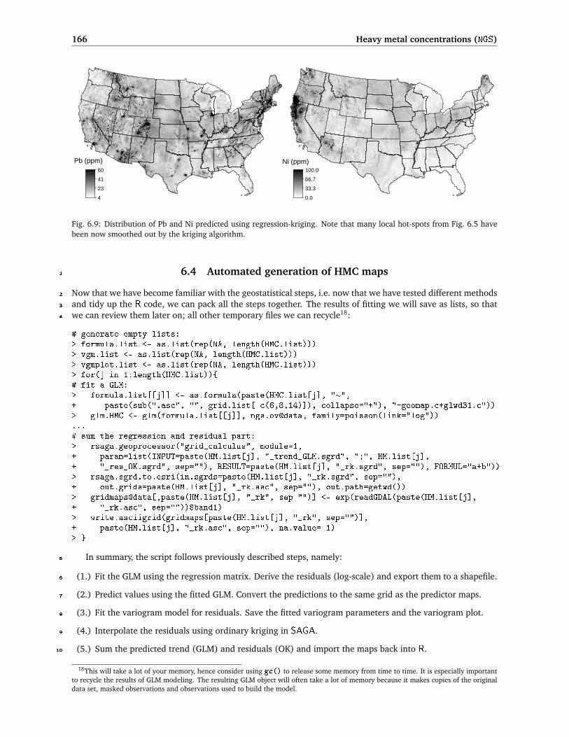
166 Heavy metal concentrations (NGS)
60
41
23
4
Pb (ppm)100.0
66.7
33.3
0.0
Ni (ppm)
Fig. 6.9: Distribution of Pb and Ni predicted using regression-kriging. Note that many local hot-spots from Fig. 6.5 havebeen now smoothed out by the kriging algorithm.
6.4 Automated generation of HMC maps1
Now that we have become familiar with the geostatistical steps, i.e. now that we have tested different methods2
and tidy up the R code, we can pack all the steps together. The results of fitting we will save as lists, so that3
we can review them later on; all other temporary files we can recycle18:4
# generate empty lists:> formula.list <- as.list(rep(NA, length(HMC.list)))> vgm.list <- as.list(rep(NA, length(HMC.list)))> vgmplot.list <- as.list(rep(NA, length(HMC.list)))> for(j in 1:length(HMC.list)){# fit a GLM:> formula.list[[j]] <- as.formula(paste(HMC.list[j], "∼",+ paste(sub(".asc", "", grid.list[-c(6,8,14)]), collapse="+"), "+geomap.c+glwd31.c"))> glm.HMC <- glm(formula.list[[j]], ngs.ov@data, family=poisson(link="log"))...# sum the regression and residual part:> rsaga.geoprocessor("grid_calculus", module=1,+ param=list(INPUT=paste(HM.list[j], "_trend_GLM.sgrd", ";", HM.list[j],+ "_res_OK.sgrd", sep=""), RESULT=paste(HM.list[j], "_rk.sgrd", sep=""), FORMUL="a+b"))> rsaga.sgrd.to.esri(in.sgrds=paste(HM.list[j], "_rk.sgrd", sep=""),+ out.grids=paste(HM.list[j], "_rk.asc", sep=""), out.path=getwd())> gridmaps@data[,paste(HM.list[j], "_rk", sep="")] <- exp(readGDAL(paste(HM.list[j],+ "_rk.asc", sep=""))$band1)> write.asciigrid(gridmaps[paste(HM.list[j], "_rk", sep="")],+ paste(HM.list[j], "_rk.asc", sep=""), na.value=-1)> }
In summary, the script follows previously described steps, namely:5
(1.) Fit the GLM using the regression matrix. Derive the residuals (log-scale) and export them to a shapefile.6
(2.) Predict values using the fitted GLM. Convert the predictions to the same grid as the predictor maps.7
(3.) Fit the variogram model for residuals. Save the fitted variogram parameters and the variogram plot.8
(4.) Interpolate the residuals using ordinary kriging in SAGA.9
(5.) Sum the predicted trend (GLM) and residuals (OK) and import the maps back into R.10
18This will take a lot of your memory, hence consider using gc() to release some memory from time to time. It is especially importantto recycle the results of GLM modeling. The resulting GLM object will often take a lot of memory because it makes copies of the originaldata set, masked observations and observations used to build the model.

6.4 Automated generation of HMC maps 167
(6.) Back-transform the values to the original scale; export the map to a GIS format. 1
distance (m)
sem
ivar
ianc
e
0.05
0.10
0.15
0.20
0.25
5000 15000 25000
+
++ + +
++ + + + + + +
+ +
As
distance (m)
sem
ivar
ianc
e
0.01
0.02
0.03
0.04
0.05
5000 15000 25000
+ +
+ ++
+ ++
++
+ + + + +
Cd
distance (m)
sem
ivar
ianc
e
0.1
0.2
0.3
0.4
0.5
5000 15000 25000
+
++
+ ++ + + + + + + + + +
Cr
distance (m)
sem
ivar
ianc
e
0.05
0.10
0.15
0.20
0.25
0.30
5000 15000 25000
+ +
+ + + + + + ++ + + + + +
Cu
distance (m)
sem
ivar
ianc
e
0.1
0.2
0.3
5000 15000 25000
+
++ + +
+ + + + + + + ++ +
Ni
distance (m)
sem
ivar
ianc
e
0.05
0.10
0.15
0.20
5000 15000 25000
++
++ +
+ + + + + + + + + +
Zn
distance (m)
sem
ivar
ianc
e
0.05
0.10
0.15
0.20
0.25
0.30
5000 15000 25000
+
++ +
+ + ++ + + + +
+ + +
As(2)
distance (m)
sem
ivar
ianc
e
0.005
0.010
0.015
5000 15000 25000
++
+
+++
+
++
+
+++
++
Hg
distance (m)
sem
ivar
ianc
e0.05
0.10
0.15
0.20
0.25
0.30
5000 15000 25000
+
++
+ + + + + + + + + + + +
Pb
Fig. 6.10: Variograms fitted for GLM residuals.
To review the results of model fitting we can best look at the fitted variograms (Fig. 6.10). If the variograms 2
are stable and fitted correctly, and if they do not exceed the physical range of values, we can be confident that 3
the predictions will be meaningful. In this case, we can see that all variograms have a standard shape, except 4
for Hg, which seems to show close to pure nugget effect. We can repeat the variogram fitting by-eye for this 5
HMC, and then re-interpolate the data, at least to minimize artifacts in the final map. Note also that the nugget 6
variation is significant for all variables. 7
The final predictions for various HMCs can be used to extract the principal components, i.e. reduce eight 8
maps to two maps. Recall from Fig. 6.3 that there are basically two big groups of HMCS: Zn, Cu, Ni, Cr; 9
and As, Pb, Hg, Cd. The first component derived using these maps is shown in Fig. 6.11. This map can be 10
considered to show the overall pollution by HMCs with ‘industrial’ origin (As, Pb, Hg and Cd) for the whole of 11
USA. 12
Based on the results of analysis, we can conclude the following. First, auxiliary maps such as density of 13
toxic releases, urbanization intensity, geology and similar, can be used to improve interpolation of various 14
heavy metals. For example, distribution of Pb can be largely explained by density of toxic releases and night 15
light images, several heavy metals can be explained by geological soil mapping units. Second, selected heavy 16
metals are positively correlated — principal component plots for NGS are similar to the results of the European 17
case study (Rodriguez Lado et al., 2009). Third, most of HMCs have distributions skewed towards low values. 18
This proves that HMCs can in general be considered to follow a Poisson-type distribution. 19
This results also confirm that some local hot-spots shown in Fig. 6.5 are not really probable, and therefore 20
have been smoothed out (compare with Fig. 6.9). Interpolation of some HMCs is not trivial. Mercury is, for 21
example, a difficult element for which to obtain accurate analyzes (Grossman et al., 2008). Samples can easily 22
be contaminated with Hg during handling, storage, and preparation for analysis. 23

168 Heavy metal concentrations (NGS)
Fig. 6.11: First principal component derived using a stack of predicted maps of eight heavy metals. This PC basicallyrepresents mapped overall concentration of As, Pb and Cd (compare with Fig. 6.3); shown as a ground overlay in Google
Earth.
6.5 Comparison of ordinary and regression-kriging1
Finally we can also run a comparison between OK and RK methods to analyze the benefits of using auxiliary2
predictors (or are there benefits at all)? The recommended software to run such analysis is geoR, because it3
is more suited to analyzing skewed variables, and because it provides more insight into the results of model4
fitting. To speed up processing, we can focus on two US states (Illinois and Indiana) and only the most5
significant predictors. We can subset (using the bounding box coordinates) the auxiliary maps using:6
# subset the original predictors:> grid.list.s <- c("dairp.asc", "dTRI.asc", "nlights03.asc", "sdroads.asc")> rsaga.esri.to.sgrd(in.grids=grid.list.s, out.sgrds=set.file.extension(grid.list.s,+ ".sgrd"), in.path=getwd())> for(i in 1:length(grid.list.s)) {# first, create a new grid:> rsaga.geoprocessor(lib="grid_tools", module=23, param=list(GRID="tmp2.sgrd",+ M_EXTENT=1, XMIN=360000, YMIN=1555000, XMAX=985000, YMAX=2210000, CELLSIZE=5000))# 0.01 decimal places:> rsaga.geoprocessor("grid_calculus", module=1, param=list(INPUT="tmp2.sgrd",+ RESULT=paste("m_", set.file.extension(grid.list.s[i], ".sgrd"), sep=""),+ FORMUL="a/100")) # 0.01 decimal places# now, resample all grids:> rsaga.geoprocessor(lib="grid_tools", module=0,+ param=list(INPUT=set.file.extension(grid.list.s[i], ".sgrd"),+ GRID=paste("m_", set.file.extension(grid.list.s[i], ".sgrd"), sep=""),+ GRID_GRID=paste("m_", set.file.extension(grid.list.s[i], ".sgrd"), sep=""),+ METHOD=2, KEEP_TYPE=FALSE, SCALE_DOWN_METHOD=0))> }> rsaga.sgrd.to.esri(in.sgrds=paste("m_", set.file.extension(grid.list.s, ".sgrd"),+ sep=""), out.grids=paste("m_", set.file.extension(grid.list.s, ".asc"),+ sep=""), out.path=getwd(), pre=3)# read maps into R:> gridmaps.s <- readGDAL(paste("m_", set.file.extension(grid.list.s[1], ".asc"), sep=""))> for(i in 2:length(grid.list.s)) {
6.5 Comparison of ordinary and regression-kriging 169
> gridmaps.s@data[i] <- readGDAL(paste("m_", set.file.extension(grid.list.s[i],+ ".asc"), sep=""))$band1> }> names(gridmaps.s) <- sub(".asc", "", grid.list.s)> str(gridmaps.s@data)
'data.frame': 16632 obs. of 4 variables:$ dairp : num 0.031 0.03 0.031 0.032 0.033 ...$ dTRI : num 0.007 0.007 0.007 0.008 0.008 ...$ nlights03: num 6 3 6 2 0 4 5 16 5 5 ...$ sdroads : num 0 0 7497 0 0 ...
which has resampled the original grids to a 125×131 pixels block. We also need to subset the point data (we 1
focus on Pb) using the same window (Xmin=360000, Xmax=985000, Ymin=1555000, Ymax=2210000) with the 2
help of SAGA module shapes_tools: 3
# subset the point data:> rsaga.geoprocessor(lib="shapes_tools", module=14,+ param=list(SHAPES="PB_ICP40.shp", CUT="m_PB_ICP40.shp", METHOD=0, TARGET=0,+ CUT_AX=360000, CUT_BX=985000, CUT_AY=1555000, CUT_BY=2210000))> m_PB <- readOGR("m_PB_ICP40.shp", "m_PB_ICP40")
OGR data source with driver: ESRI ShapefileSource: "m_PB_ICP40.shp", layer: "m_PB_ICP40"with 2787 rows and 1 columnsFeature type: wkbPoint with 2 dimensions
which limits the analysis to only 2787 points within the area of interest. We convert the data to the native 4
geoR format: 5
> Pb.geo <- as.geodata(m_PB["PB_ICP40"])
as.geodata: 622 redundant locations foundWARNING: there are data at coincident or very closed locations, some of the geoR'sfunctions may not work. Use function dup.coords to locate duplicated coordinates.
which shows that there might be some problems for further analysis because there are many duplicate points 6
and the calculation might fail due to singular matrix problems. Even though the data set is much smaller than 7
the original NGS data set, geoR might still have problems running any analysis. Hence, a good idea is to (1) 8
remove duplicates, and (2) randomly subset point data: 9
> m_PB <- remove.duplicates(m_PB)> str(Pb.geo[[2]])
num [1:2165] 9 10 10 9 16 14 8 15 11 9 ...
> m_PB.ov <- overlay(gridmaps.s, m_PB)# subset to speed up:> sel <- runif(length(m_PB@data[[1]]))<0.5> Pb.geo1 <- as.geodata(m_PB[sel, "PB_ICP40"])> str(Pb.geo1[[2]])
num [1:1120] 9 10 14 11 11 18 14 13 10 8 ...
# copy values of covariates:> Pb.geo1$covariate <- m_PB.ov@data[sel, sub(".asc", "", grid.list.s)]
We can now proceed with variogram modeling. First, we estimate the variogram for the original variable: 10
> Pb.vgm <- likfit(Pb.geo1, lambda=0, messages=FALSE, ini=c(var(log1p(Pb.geo$data)),+ 50000), cov.model="exponential")> Pb.vgm
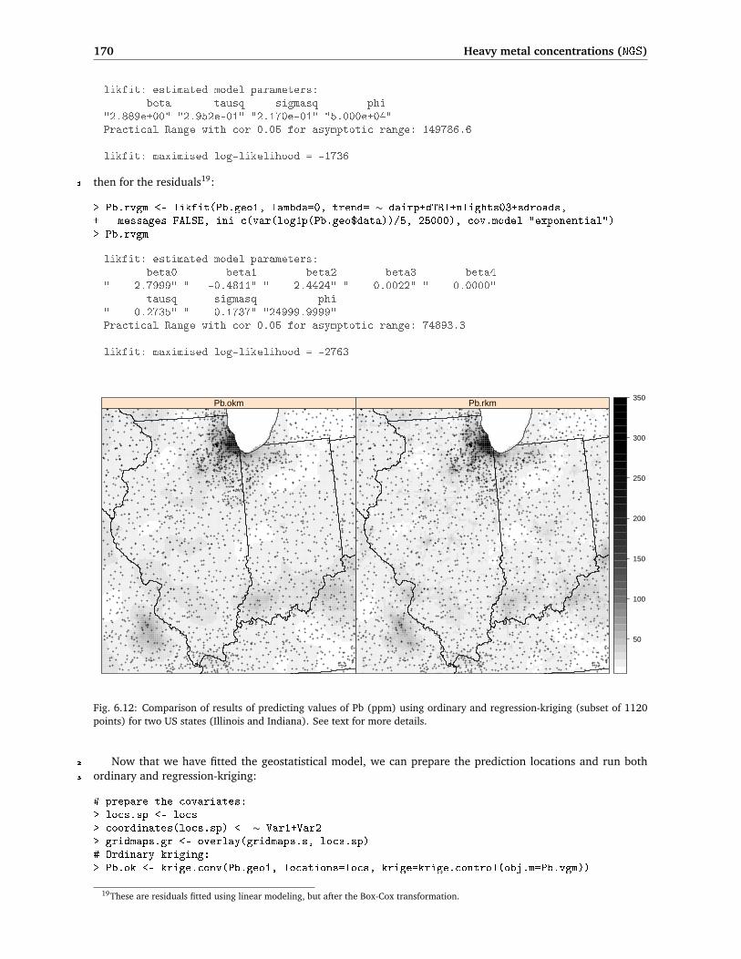
170 Heavy metal concentrations (NGS)
likfit: estimated model parameters:beta tausq sigmasq phi
"2.889e+00" "2.952e-01" "2.170e-01" "5.000e+04"Practical Range with cor=0.05 for asymptotic range: 149786.6
likfit: maximised log-likelihood = -1736
then for the residuals19:1
> Pb.rvgm <- likfit(Pb.geo1, lambda=0, trend= ∼ dairp+dTRI+nlights03+sdroads,+ messages=FALSE, ini=c(var(log1p(Pb.geo$data))/5, 25000), cov.model="exponential")> Pb.rvgm
likfit: estimated model parameters:beta0 beta1 beta2 beta3 beta4
" 2.7999" " -0.4811" " 2.4424" " 0.0022" " 0.0000"tausq sigmasq phi
" 0.2735" " 0.1737" "24999.9999"Practical Range with cor=0.05 for asymptotic range: 74893.3
likfit: maximised log-likelihood = -2763
+++ +
+
+ ++
+
+
+
+ +
++
+
+ +++++ + +
++
+ ++++
++
+
++
++
+ +
+++
+++
++
++
++ ++
++
++
+
+++++ + +
++
++
++
+ +++
+
++ +
++
++
++ ++
++
+
+ ++
+
++
+ +
+++ +
++
+
+++
+
+ ++
+
+
+
+ ++
+ +
+
+ +
+ +
++
++
+
++
+
+
+
+
+
+
+
+
+ ++
+
+
+
++
+
+
+
+
+
+
++
+
+
+
+
++
+
+
+
+
+
+
+
+
++
+
+
++
+
+
+
+
+ +
+
+
+
+
+
+
+
+
+
+
+
++
+
+
+
++
+
+
+
+
+
+
++
++
+
+
+
+
++
++
+
+
+
+
+
+
+
+
+
++
+
+
+
+
+
+
++
+
+
++
+
+
+
+
+
+
+
+
++
+
+
+
+
+
+
+
++
+
+
+
+++
+
+
+
+
+
+
+
+
+
+
+
++
+
+
+
+
++
+
+
+
+
+
+
+
+
+
+
+
+
+
+
+
+
+
+
+
++
+
+
++
+
++
+
+
+
+
+
+
+
+
+
+
+
++ +
++
+
+ ++
+
+
+
+ +
+
+
+
++
+
+
+ +
++
+
+
++
+
+
++
+
+
+
+
+
+
+
++
+
+
+ ++
+
++
+
+
+
+
+
+
+
+
+
+
+
+
+
+
++
+
+
+
+
+++
+
+
+
+
+
+ ++++
+
+
++
+
+
+
+
+
++
++
++
++
++ +
+
++
+
+
+ ++
+
+
++ +
+
+
++
+
+
+
+
+
++
+
+
+ +
+
+
+
++
+
+
+
+
+
++
+
+
++
+
+
+
++ +
+
+
++
+
++ +
++
+
++
+
+
+
+
+
+
++
++
+
+
+ +
+
+
+
+
+
+
+
+
++
+
+
+
+
+
+
+
+
+
+
+ +
++
++
+
+
+
+
+
+
+
+
+
+
+
+
+
+
+
+
+
+
+
+
+
+
+
+
+
+
+
+
+
+
+
+
+ +
++
++
+
+
++
+
+
+
+
+
+
+
+
+
+
+
+
+
+
+
+
+
+
+
+
++ +
+
+
+
+
+
+
+
+
++
+
+
+
+
+
+
+
+
+
++
+
+
+
+
+
+
+
+
+
+
+
+
+
+
+
+
+
+
+
+
+
+
++
+
+
+
+
+
+
+
+
+
+
+
+
+
+
+
+
+
+
+
+
+
+
+
+
++
++
+
+
+
+
+
+
++
+
+
+
+
+
+
+
+
+
+
+
+
+
+
+
+
+
+
+
+
+
+
+
+
+
+
+
+
+
+
+
+
+
+
+
+
+
+
+
+
+
++
+
++
++
+
+
+
+
+
+
+
+
+
+
+
+
+
+
+
+
+
+
+
+
++
+
+
++
+
+ +
+
+
+
+
+
+
+
+
+
+
+
++
+
+
++
+
+
+
+
+
+
+
+
+
+
+
+
++
+
+
+
++
+
++
+
+
+
+
+
++
+
+
+
+
+
+
+
+
+
+
+
+
+
+
+
+
+
+
+
+
+
+
+
+
+
+
+
+
+
+
+
+
+
+
+
+
+ +
++
+
+
+
+
+
+
+
+
+ +
+
+
+
+
+
+
+
+
+
+
+
+
+
+
+
+
+
++
+
+
+
+
+
+
+
+
+ + +
+
+
+
+
+
+
+
+
+
+
+
++
+
+
+
+
+
+
+
+
+
+
+
+
+
+
+
+
+
+
+
+
+
+
+
+
+
+
+
+
+
+
+
+
+
+
+
+
+
+
+
+
+
+
+
+
+
+
+
+
+
+
+
+
+
+
+
+
+
+
+
+
+
+
+
+
+
+
+
+
+
+
++
+
+
+
+
+
+
+
+
+
+
+
+
+
+
+
+
+
++
+
+
+
++
+
++
+
+
+
+
+
+
+
+
+
+
+
+
+
+
+
+
+
+
+
+
+
+
+
+
+
++
+
++
+
++
+
+
+
+
+
+
+
+
++
+
+
+
+
+
+
+
+
+
+
++
+
+
+
+
+
+
+
+
+
++
+
+
++
+
+
+
+
++
+
+
++
+
+
+
+
+
+
+
+
++
+
+
++
+
+
++
+
+
+
+
+
+
++
+
+
+
+
+
+
+
+
+
+
+
+
++
+
+
+
++
+
+
++
+
+ +
+
+
+
+
+
+
+
++
+
++
+
+
+++
+
+
+
+
+
+ +
+
+
++
+
+
+ +
+
+
+
+
+
+
+
++ +
+
++ +
+
+
+
++
+
++
++
+
++
+
++
+
+
+
+
+
+ ++
+
+
+
+
+
+
+
+
+
+
+
+
+
+
+
+
+
+
+
+
+
+
+ ++
+
+
+
+
+++ ++
+
+
+
+
+
+
+
+
+
+
+
+
+
++
+
+
+
+
+
+
+
++
+
+
+
+++
+
+
+
+
+
+
+
+
++
+
+
+
+
++
+
+
+
+
+
+
+
+
+
++
++
+ +
++
++
+
+
+
+
++
+
+
+
+
+
+
+
+
+
+
+
++
+
+
+
+
+ +
+
+ ++
+
+
+
+
++
+
+
+
+
+
+
+
+ +
++
+
+
+
+
+
+
+
+
+
+
+
+
++
++
+
+
++
+
++
+
++
+
+
+
++
+
+
+
+++++++++++
++
+
+
+++
+
+
+
+
+
+
+
+
+++
+
+++
+++
++
+
++
+
++
++
+++++++++++
+
+
++
+
+++
+
+
+
+
+
+
+
+
+
+
+
+
+
+
+
+
+
+
+
+
++
+
+
+
+
+
+
+
+
+
+
+
+
+
+
+
+
+
+
+
+
+
+
+
+
+
+
+
+
+
+
+
+
+
+
+
+
+
+
+
+
+
+
+
+
+
+
+
+
+
+
+
+
+
+
+
+
+
+
+
+
+
+
+
+
+
+
+
+
+
+
+
+
+
+
+
+
+
+
+
+
+
+
+
+
+
+
+
+
+
+
+
+
+
++
+
+
+
+
+
+
+
+
+
+
+
+
+
+
+
+
+
+
+
++
+
+
+
+
+
+
+
+
+
+
+
+ +
+
+
+
+
+
+
++
+
+
+
+
+
+
+
+
+
+
+
+
+
+
+
+
+
+
+
+
+
+
+
+
+
+
+
+
+
+
+
+
+
+
+
+
+
+
++
+
+
+
+
+
+
+
+
+
+
+
+
+
+
+
+
+
+
+
+
+
+
+
+
+
+
+
+
+
+
+
+
+
+
+
+
+
+
+
+
+
+
+
+
+
+
+
+
+
+
+
+
++
+
+
++
+
++
+
+
+
+
+
+
++
+
+
+
+
+
+
+
+
+
+
+
+
+
+
+
+
+
+
+
+
+
+
+
+
+
+
+
+
+
+
+
+
+
+
+
++
+
+
+
+
+
+
+
+
+
+
+
++
+
+
+
+ +
+
+
+
+
+
+
+
++
+
+
+
+
+
+
+
+
+
+
+
+
+
+
+
+
+
++
+
+
+
+
+
+
+
+
+
+
+
+
+
+
+
+
+
+
+
++
+
+
+
+
+
+
+
+
+
+
+
+
+ + +
+
+
+
+
+ +
++
+
+
+
+
+
+
+
+
+
+
+
++
+
+
+
++
+
+
+
+
+
+
++
+
+
+
+
+
++
+
+
+
+
++
+
+
+
+
+
+
+
+
+
+
+
+
+
+
+
+
+
+
+
+
+
+
+
+
+
+
+
+
+
+
+
+
+
+
+
++
+++ ++
+ ++ + ++ +
+ +
+ +++
++ +
++
++ +
+ +
+ ++++
+
++
++ ++ +
+ +++
+ ++ ++
+ ++
+ ++++ + ++ +
++
+ + ++
++
++
+ +
+ + ++
++
++++ + + +
++
+
+
++
+
+
+
+
+++ +
+
++
++
+
++
+
+
+
+
+
++
+ ++
+ +
+
+ +++
+ + + ++
+ ++
++ ++
+
+
++
+ + +++
+ ++ + +
++
++ ++
+
+
+
+
++
+
++
+ + +
++ +
++ ++
++
++ +
++
+ ++
+
+
+ + ++++ + +
+ +++
+ ++ + + + + +
++
++
+ +++
+ + + +
+++
+
+
++
++
+ + +
++
+
+++++
+
++
++
++
++
+
+++
++
Pb.okm+++ +
+
+ ++
+
+
+
+ +
++
+
+ +++++ + +
++
+ ++++
++
+
++
++
+ +
+++
+++
++
++
++ ++
++
++
+
+++++ + +
++
++
++
+ +++
+
++ +
++
++
++ ++
++
+
+ ++
+
++
+ +
+++ +
++
+
+++
+
+ ++
+
+
+
+ ++
+ +
+
+ +
+ +
++
++
+
++
+
+
+
+
+
+
+
+
+ ++
+
+
+
++
+
+
+
+
+
+
++
+
+
+
+
++
+
+
+
+
+
+
+
+
++
+
+
++
+
+
+
+
+ +
+
+
+
+
+
+
+
+
+
+
+
++
+
+
+
++
+
+
+
+
+
+
++
++
+
+
+
+
++
++
+
+
+
+
+
+
+
+
+
++
+
+
+
+
+
+
++
+
+
++
+
+
+
+
+
+
+
+
++
+
+
+
+
+
+
+
++
+
+
+
+++
+
+
+
+
+
+
+
+
+
+
+
++
+
+
+
+
++
+
+
+
+
+
+
+
+
+
+
+
+
+
+
+
+
+
+
+
++
+
+
++
+
++
+
+
+
+
+
+
+
+
+
+
+
++ +
++
+
+ ++
+
+
+
+ +
+
+
+
++
+
+
+ +
++
+
+
++
+
+
++
+
+
+
+
+
+
+
++
+
+
+ ++
+
++
+
+
+
+
+
+
+
+
+
+
+
+
+
+
++
+
+
+
+
+++
+
+
+
+
+
+ ++++
+
+
++
+
+
+
+
+
++
++
++
++
++ +
+
++
+
+
+ ++
+
+
++ +
+
+
++
+
+
+
+
+
++
+
+
+ +
+
+
+
++
+
+
+
+
+
++
+
+
++
+
+
+
++ +
+
+
++
+
++ +
++
+
++
+
+
+
+
+
+
++
++
+
+
+ +
+
+
+
+
+
+
+
+
++
+
+
+
+
+
+
+
+
+
+
+ +
++
++
+
+
+
+
+
+
+
+
+
+
+
+
+
+
+
+
+
+
+
+
+
+
+
+
+
+
+
+
+
+
+
+
+ +
++
++
+
+
++
+
+
+
+
+
+
+
+
+
+
+
+
+
+
+
+
+
+
+
+
++ +
+
+
+
+
+
+
+
+
++
+
+
+
+
+
+
+
+
+
++
+
+
+
+
+
+
+
+
+
+
+
+
+
+
+
+
+
+
+
+
+
+
++
+
+
+
+
+
+
+
+
+
+
+
+
+
+
+
+
+
+
+
+
+
+
+
+
++
++
+
+
+
+
+
+
++
+
+
+
+
+
+
+
+
+
+
+
+
+
+
+
+
+
+
+
+
+
+
+
+
+
+
+
+
+
+
+
+
+
+
+
+
+
+
+
+
+
++
+
++
++
+
+
+
+
+
+
+
+
+
+
+
+
+
+
+
+
+
+
+
+
++
+
+
++
+
+ +
+
+
+
+
+
+
+
+
+
+
+
++
+
+
++
+
+
+
+
+
+
+
+
+
+
+
+
++
+
+
+
++
+
++
+
+
+
+
+
++
+
+
+
+
+
+
+
+
+
+
+
+
+
+
+
+
+
+
+
+
+
+
+
+
+
+
+
+
+
+
+
+
+
+
+
+
+ +
++
+
+
+
+
+
+
+
+
+ +
+
+
+
+
+
+
+
+
+
+
+
+
+
+
+
+
+
++
+
+
+
+
+
+
+
+
+ + +
+
+
+
+
+
+
+
+
+
+
+
++
+
+
+
+
+
+
+
+
+
+
+
+
+
+
+
+
+
+
+
+
+
+
+
+
+
+
+
+
+
+
+
+
+
+
+
+
+
+
+
+
+
+
+
+
+
+
+
+
+
+
+
+
+
+
+
+
+
+
+
+
+
+
+
+
+
+
+
+
+
+
++
+
+
+
+
+
+
+
+
+
+
+
+
+
+
+
+
+
++
+
+
+
++
+
++
+
+
+
+
+
+
+
+
+
+
+
+
+
+
+
+
+
+
+
+
+
+
+
+
+
++
+
++
+
++
+
+
+
+
+
+
+
+
++
+
+
+
+
+
+
+
+
+
+
++
+
+
+
+
+
+
+
+
+
++
+
+
++
+
+
+
+
++
+
+
++
+
+
+
+
+
+
+
+
++
+
+
++
+
+
++
+
+
+
+
+
+
++
+
+
+
+
+
+
+
+
+
+
+
+
++
+
+
+
++
+
+
++
+
+ +
+
+
+
+
+
+
+
++
+
++
+
+
+++
+
+
+
+
+
+ +
+
+
++
+
+
+ +
+
+
+
+
+
+
+
++ +
+
++ +
+
+
+
++
+
++
++
+
++
+
++
+
+
+
+
+
+ ++
+
+
+
+
+
+
+
+
+
+
+
+
+
+
+
+
+
+
+
+
+
+
+ ++
+
+
+
+
+++ ++
+
+
+
+
+
+
+
+
+
+
+
+
+
++
+
+
+
+
+
+
+
++
+
+
+
+++
+
+
+
+
+
+
+
+
++
+
+
+
+
++
+
+
+
+
+
+
+
+
+
++
++
+ +
++
++
+
+
+
+
++
+
+
+
+
+
+
+
+
+
+
+
++
+
+
+
+
+ +
+
+ ++
+
+
+
+
++
+
+
+
+
+
+
+
+ +
++
+
+
+
+
+
+
+
+
+
+
+
+
++
++
+
+
++
+
++
+
++
+
+
+
++
+
+
+
+++++++++++
++
+
+
+++
+
+
+
+
+
+
+
+
+++
+
+++
+++
++
+
++
+
++
++
+++++++++++
+
+
++
+
+++
+
+
+
+
+
+
+
+
+
+
+
+
+
+
+
+
+
+
+
+
++
+
+
+
+
+
+
+
+
+
+
+
+
+
+
+
+
+
+
+
+
+
+
+
+
+
+
+
+
+
+
+
+
+
+
+
+
+
+
+
+
+
+
+
+
+
+
+
+
+
+
+
+
+
+
+
+
+
+
+
+
+
+
+
+
+
+
+
+
+
+
+
+
+
+
+
+
+
+
+
+
+
+
+
+
+
+
+
+
+
+
+
+
+
++
+
+
+
+
+
+
+
+
+
+
+
+
+
+
+
+
+
+
+
++
+
+
+
+
+
+
+
+
+
+
+
+ +
+
+
+
+
+
+
++
+
+
+
+
+
+
+
+
+
+
+
+
+
+
+
+
+
+
+
+
+
+
+
+
+
+
+
+
+
+
+
+
+
+
+
+
+
+
++
+
+
+
+
+
+
+
+
+
+
+
+
+
+
+
+
+
+
+
+
+
+
+
+
+
+
+
+
+
+
+
+
+
+
+
+
+
+
+
+
+
+
+
+
+
+
+
+
+
+
+
+
++
+
+
++
+
++
+
+
+
+
+
+
++
+
+
+
+
+
+
+
+
+
+
+
+
+
+
+
+
+
+
+
+
+
+
+
+
+
+
+
+
+
+
+
+
+
+
+
++
+
+
+
+
+
+
+
+
+
+
+
++
+
+
+
+ +
+
+
+
+
+
+
+
++
+
+
+
+
+
+
+
+
+
+
+
+
+
+
+
+
+
++
+
+
+
+
+
+
+
+
+
+
+
+
+
+
+
+
+
+
+
++
+
+
+
+
+
+
+
+
+
+
+
+
+ + +
+
+
+
+
+ +
++
+
+
+
+
+
+
+
+
+
+
+
++
+
+
+
++
+
+
+
+
+
+
++
+
+
+
+
+
++
+
+
+
+
++
+
+
+
+
+
+
+
+
+
+
+
+
+
+
+
+
+
+
+
+
+
+
+
+
+
+
+
+
+
+
+
+
+
+
+
++
+++ ++
+ ++ + ++ +
+ +
+ +++
++ +
++
++ +
+ +
+ ++++
+
++
++ ++ +
+ +++
+ ++ ++
+ ++
+ ++++ + ++ +
++
+ + ++
++
++
+ +
+ + ++
++
++++ + + +
++
+
+
++
+
+
+
+
+++ +
+
++
++
+
++
+
+
+
+
+
++
+ ++
+ +
+
+ +++
+ + + ++
+ ++
++ ++
+
+
++
+ + +++
+ ++ + +
++
++ ++
+
+
+
+
++
+
++
+ + +
++ +
++ ++
++
++ +
++
+ ++
+
+
+ + ++++ + +
+ +++
+ ++ + + + + +
++
++
+ +++
+ + + +
+++
+
+
++
++
+ + +
++
+
+++++
+
++
++
++
++
+
+++
++
Pb.rkm
50
100
150
200
250
300
350
Fig. 6.12: Comparison of results of predicting values of Pb (ppm) using ordinary and regression-kriging (subset of 1120points) for two US states (Illinois and Indiana). See text for more details.
Now that we have fitted the geostatistical model, we can prepare the prediction locations and run both2
ordinary and regression-kriging:3
# prepare the covariates:> locs.sp <- locs> coordinates(locs.sp) <- ∼ Var1+Var2> gridmaps.gr <- overlay(gridmaps.s, locs.sp)# Ordinary kriging:> Pb.ok <- krige.conv(Pb.geo1, locations=locs, krige=krige.control(obj.m=Pb.vgm))
19These are residuals fitted using linear modeling, but after the Box-Cox transformation.

6.5 Comparison of ordinary and regression-kriging 171
krige.conv: model with constant meankrige.conv: performing the Box-Cox data transformationkrige.conv: back-transforming the predicted mean and variancekrige.conv: Kriging performed using global neighbourhood
# Regression-kriging:> KC <- krige.control(trend.d = ∼ dairp+dTRI+nlights03+sdroads, trend.l =+ ∼ gridmaps.gr$dairp+gridmaps.gr$dTRI+gridmaps.gr$nlights03+gridmaps.gr$sdroads,+ obj.m = Pb.rvgm)> Pb.rk <- krige.conv(Pb.geo1, locations=locs, krige=KC)
krige.conv: model with mean defined by covariates provided by the userkrige.conv: performing the Box-Cox data transformationkrige.conv: back-transforming the predicted mean and variancekrige.conv: Kriging performed using global neighbourhood
This time we did not use any mask (border coordinates), so that we need to mask the water bodies after 1
converted the data to sp class (compare with §5.5.3): 2
# sp plot:> locs.geo <- data.frame(X=locs.sp@coords[,1], Y=locs.sp@coords[,2],+ Pb.rk=Pb.rk[[1]], Pb.ok=Pb.ok[[1]], Pb.rkvar=Pb.rk[[2]], Pb.okvar=Pb.ok[[2]])> coordinates(locs.geo) <- ∼ X+Y> gridded(locs.geo) <- TRUE# mask out water bodies:> mask.s <- as.vector(t(as.im(gridmaps.s["geomap"])$v)) # flip pixels up-side down> locs.geo$Pb.ok <- ifelse(is.na(mask.s), NA, locs.geo$Pb.ok)> locs.geo$Pb.rk <- ifelse(is.na(mask.s), NA, locs.geo$Pb.rk)> spplot(locs.geo[c("Pb.ok", "Pb.rk")], col.regions=grey(rev(seq(0,1,0.025)^2)),+ at=seq(5,350,l=40), sp.layout=list(list("sp.points", m_PB, pch="+", col="black"),+ list("sp.lines", USA.borders, col="black")))> summary(locs.geo$Pb.okvar)
Min. 1st Qu. Median Mean 3rd Qu. Max.25.91 145.80 198.40 336.10 271.00 26860.00
> summary(locs.geo$Pb.rkvar)
Min. 1st Qu. Median Mean 3rd Qu. Max.22.13 144.10 190.40 306.50 258.60 42200.00
The results are illustrated in Fig. 6.12. RK does seem to be more efficient in reflecting the spatial pattern 3
of industrial activities and pollution sources. The range of values in the map predicted using RK is somewhat 4
higher, which is due the fact that we have now used geoR package that deals very well with skewed distribu- 5
tions so that many peaks, invisible in the OK predictions map, have been emphasized with RK. The prediction 6
error of RK is, as expected, somewhat smaller than for OK, but the difference is rather small (378 vs 391). 7
This is also because the prediction error of the RK is proportionally higher in areas with high values, so that 8
the overall average error is higher. 9
Self-study exercises: 10
(1.) At which locations are the maps shown in Fig. 6.5 and 6.9 the most different? (HINT: derive and plot a 11
difference map) 12
(2.) Which predictors are most highly correlated with each other? Plot first and second component derived 13
using all maps — what do they reflect? 14
(3.) Which HMC is the most difficult to interpolate? (HINT: look at the residuals of the regression model, 15
nugget parameter etc.) 16

172 Heavy metal concentrations (NGS)
(4.) Split the original NGS point data set based on source (stream sediments, soils etc.) and then repeat1
the analysis for at least three HMCs. Is there a difference between the regression models? (HINT: plot2
correlation lines for various media in the same graph.)3
(5.) How much does the accuracy in the HMC maps decrease if we use only 10% of samples (randomly4
selected) versus the complete data set? (HINT: use standard measures described in §1.4 to run a com-5
parison.)6
(6.) Which US state has highest concentration of Pb on average?7
(7.) Run the cross-validation following the exercise in §6.5 and see if the predictions made using RK are8
significantly better than with OK.9
(8.) Compare the accuracy of predictions for element Pb using ordinary kriging on untransformed data and10
using the Box–Cox transformation — are there significant differences? (HINT: randomly split the NGS11
data set to two equal size data sets; then use one for validation only.)12
Further reading:13
Æ Grossman, J. N. and Grosz, A. E. and Schweitzer, P. N. and Schruben, P. G., 2008. The National Geo-14
chemical Survey — Database and Documentation, Version 5. U.S. Geological Survey, Reston, VA.15
Æ Papritz, A. and Reichard, P. U., 2009. Modeling the risk of Pb and PAH intervention value exceedance in16
allotment soils by robust logistic regression. Environmental Pollution, 157(7): 2019–2022.17
Æ Reimann, C., Filzmoser, P., Garrett, R., Dutter, R., 2008. Statistical Data Analysis Explained Applied18
Environmental Statistics with R. Wiley, Chichester, 337 p.19
Æ Rodriguez Lado, L. and Hengl, T. and Reuter, H. I., 2009. Heavy metals in European soils: a geostatistical20
analysis of the FOREGS Geochemical database. Geoderma, 148(2): 189–199.21
Æ http://tin.er.usgs.gov/geochem/ — The National Geochemical Survey website.22
Æ http://www.gtk.fi/publ/foregsatlas/ — The Geochemical atlas of Europe.23

7 1
Soil Organic Carbon (WISE_SOC) 2
7.1 Introduction 3
ISRIC WISE is an international soil profile data set; a selection of globally distributed soil profiles, prepared 4
by the International Soil Reference and Information Centre (ISRIC) located in Wageningen (Batjes, 2008, 5
2009). The most recent version (3.1) of the soil profile database contains 10,253 profiles1. The database 6
consists of several tables, the most important are: WISE3_SITE (information about the soil profile site) and 7
WISE3_HORIZON (laboratory data per horizon). This chapter demonstrates how to estimate the global Soil 8
Organic Carbon (SOC) stock using regression-kriging and a large repository of publicly accessible global 9
environmental maps (about 10 km resolution) described in section 4.1. The results contribute to the Glob- 10
alSoilMap.net initiative that aims at producing high resolution images of key soil properties and functions 11
(Sanchez et al., 2009). 12
The maps presented in this exercise were created for demonstration purposes only. The true accuracy/- 13
consistency of these maps has not been evaluated and is heavily controlled by the representativeness of the 14
sampling pattern and accuracy of individual measurements (refer to the ISRIC WISE general disclaimer2). 15
Positional accuracy of profiles in WISE varies depending on the source materials from which they were de- 16
rived — this may range from the nearest second Lat/Lon up to few meters. Most of the available legacy data 17
considered in WISE date from the pre-GPS era. In addition, the list of predictors we use in this exercise could 18
be much more extensive; many of the maps are also available at finer resolutions (∼1 km). Compare also the 19
maps produced in this chapter with the global soil property maps distributed by ISRIC3, and/or the Global 20
Biomass Carbon Map produced by the CDIAC4 (Ruesch and Gibbs, 2008b). Note that this is also a relatively 21
large data set and computations can become time-consuming. It is not recommended to run this exercise using 22
a PC without at least 2 GB of RAM and at least 1 GB of hard disk memory. 23
7.2 Loading the data 24
To run this script, you first need to register and obtain the MS Access file from the ISRIC website5. Before you 25
start using the ISRIC WISE database, please also read about its limitations in Batjes (2008). Next, load the 26
necessary packages: 27
> library(RODBC)> library(gstat)> library(rgdal)> library(RSAGA)> library(spatstat)
1Not all profiles are complete.2http://www.isric.org/isric/webdocs/Docs/ISRIC_Report_2008_02.pdf3http://www.isric.org/UK/About+Soils/Soil+data/Geographic+data/Global/WISE5by5minutes.htm4http://cdiac.ornl.gov/epubs/ndp/global_carbon/carbon_documentation.html5http://www.isric.org/isric/CheckRegistration.aspx?dataset=9
173

174 Soil Organic Carbon (WISE_SOC)
For more info on how to set-up SAGA GIS and run the commands from R see section 3.1.2.1
7.2.1 Download of the world maps2
Next, download and unzip all relevant predictors from the web-repository6:3
# location of maps:> URL <- "http://spatial-analyst.net/worldmaps/"# list of maps:> map.list <- c("biocl01", "biocl02", "biocl04", "biocl05", "biocl06", "biocl12",+ "biocl15", "countries", "dcoast", "globedem", "landcov", "landmask", "gcarb",+ "nlights", "pcndvi1", "pcndvi2", "pcndvi3", "pcpopd1", "himpact", "glwd31",+ "wildness", "hwsd", "quakein", "iflworld", "treecov")# download the zipped maps one by one:> for(i in 1:length(map.list)) {> download.file(paste(URL, map.list[i], ".zip", sep=""),+ destfile=paste(getwd(), "/", map.list[i], ".zip", sep=""))> unzip(paste(getwd(), "/", map.list[i], ".zip", sep=""))> unlink(paste(map.list[i], ".zip", sep=""))# Delete temporary file:> unlink(paste(map.list[i], ".zip", sep=""))> }
trying URL 'http://spatial-analyst.net/worldmaps/biocl01.zip'Content type 'application/zip' length 1362739 bytes (1.3 Mb)opened URLdownloaded 1.3 Mb...
where biocl1-15 are long-term bioclimatic variables; dcoast is the distance from coastline; globedem is the4
ETOPO1 Global Relief Model; landcov is the Global Land Cover map of the world; landmask is the land5
mask; gcarb is the carbon (biomass) density in tones of C/ha; nlights is the long-term annual image of6
lights at night; pcndvi1/2 are first and second principal component derived from 20 years of AVHRR NDVI7
monthly images; pcpopd1 is PC1 of the Gridded Population of the World, version 3 (GPWv3), himpact is the8
world map of human impacts-free areas estimated by the GLOBIO initiative of the United Nations Environment9
Programme; glwd31 is the indicator map showing location of wetlands based on the Global Lakes and Wetlands10
Database (GWLD3.1) database; wildness is a map of the World wilderness areas; hwsd is soil class map11
based on the FAO Harmonized World Soil Database v 1.1 (37 classes); quakein is the Earthquake intensity12
(magnitude) based on the NOAA’s Significant Earthquake Database; iflworld is the world map of intact forest13
landscapes; treecov is the Vegetation percent tree cover (see also §4.1). If the download was successful, you14
will notice that the ArcInfo ASCII grids are now available in your working directory. A detailed description of15
each layer is available via the raster description (*.rdc) file. See p.159 for an example.16
We can load some maps, that we will need later on, into R using rgdal:17
> worldmaps <- readGDAL("landmask.asc")
landmask.asc has GDAL driver AAIGridand has 1300 rows and 3600 columns
> names(worldmaps) <- "landmask"> worldmaps$landcov <- as.factor(readGDAL("landcov.asc")$band1)> worldmaps$glwd31 <- as.factor(readGDAL("glwd31.asc")$band1)> worldmaps$hwsd <- as.factor(readGDAL("hwsd.asc")$band1)> proj4string(worldmaps) <- CRS("+proj=longlat +ellps=WGS84")
6http://spatial-analyst.net/worldmaps/

7.2 Loading the data 175
7.2.2 Reading the ISRIC WISE into R 1
If you have obtained the ISRIC-WISE_ver3.mdb file from ISRIC, you can connect to it by using the RODBC72
package: 3
> cGSPD <- odbcConnectAccess("ISRIC-WISE_ver3.mdb")# Look at available tables:> sqlTables(cGSPD)$TABLE_NAME
[1] "MSysAccessObjects"[2] "MSysAccessXML"[3] "MSysACEs"[4] "MSysObjects"[5] "MSysQueries"[6] "MSysRelationships"[7] "WISE3__ReadMeFirst"[8] "WISE3_coding_conventions"[9] "WISE3_HORIZON"[10] "WISE3_LABcodes_Description"[11] "WISE3_LABname"[12] "WISE3_LABname_codes"[13] "WISE3_SITE"[14] "WISE3_SOURCE"
Now that we have connected to the database, we query it to obtain values from the tables like with any 4
other SQL database. We need to obtain the following five variables: 5
ORGC = Organic carbon content in promille (or g C kg−1); 6
TOPDEP, BOTDEP = Thickness of soil horizons in cm; 7
LON, LAT = Point coordinates; 8
We first fetch measured values for organic content and the depths of each horizon from WISE3_HORIZON 9
table: 10
> GSPD.HOR <- sqlQuery(cGSPD, query="SELECT WISE3_ID, HONU, ORGC, TOPDEP,+ BOTDEP FROM WISE3_HORIZON")> str(GSPD.HOR)
'data.frame': 47833 obs. of 5 variables:$ WISE3_ID: Factor w/ 10253 levels "AF0001","AF0002",..: 1 1 1 2 2 2 2 3 3 3 ...$ HONU : int 1 2 3 1 2 3 4 1 2 3 ...$ ORGC : num 7.6 2.3 0.9 12.8 6 3.9 2.7 5.9 2.4 NA ...$ TOPDEP : int 0 15 60 0 20 60 110 0 20 50 ...$ BOTDEP : int 15 60 150 20 60 110 170 20 50 110 ...
# Horizon thickness:> GSPD.HOR$HOTH <- GSPD.HOR$BOTDEP-GSPD.HOR$TOPDEP# unique ID:> GSPD.HOR$ID <- as.factor(paste(as.character(GSPD.HOR$WISE3_ID),+ GSPD.HOR$HONU, sep="_"))
where HONU is the horizon number (from the soil surface) and TOPDEP and BOTDEP are the upper and lower 11
horizon depths. This shows that there are over 45 thousand measurements of the four variables of interest. 12
The number of soil profiles is in fact much smaller — as you can see from the WISE3_ID column (unique profile 13
ID), there are 10,253 profiles in total. 14
We know from literature that total soil organic carbon (SOC) depends on bulk density of soil and coarse 15
fragments (Batjes, 1996; Batjes et al., 2007). There is certainly a difference in how ORGC relates to SOC in 16
7http://cran.r-project.org/web/packages/RODBC/

176 Soil Organic Carbon (WISE_SOC)
volcanic soils, wetland soils, organic soils and well drained mineral soils. To correctly estimate total Soil1
Organic Carbon in kg C m−2, we can use the following formula8:2
SOC [kg m−2] =ORGC
1000[kg kg−1] ·
HOTH
100[m] · BULKDENS · 1000 [kg m−3] ·
100− GRAVEL [%]100
(7.2.1)
3
where BULKDENS is the soil bulk density9 in g cm−3 and GRAVEL is the gravel content in profile expressed in %.4
Because we are interested in total organic carbon content for soil profile, we will first estimate SOC values5
for all horizons, then aggregate these values per whole profile. Alternatively, one could try to predict organic6
carbon for various depths separately, then aggregate number of maps. Spatial analysis of soil layers makes7
sense because one can observe both shallow soils with high and low SOC content and vice versa, and these can8
both be formed under different environmental conditions. For the purpose of this exercise, we will focus only9
on the aggregate value i.e. on the total estimated soil organic carbon per profile location.10
We can load an additional table10 with Bulk density / gravel content estimated at fixed depth intervals11
(0–20, 20–40, 40–60, 60–80, 80–100, 100–150, 150–200 cm):12
> load(url("http://spatial-analyst.net/book/system/files/GSPD_BDG.RData"))> str(GSPD.BDG)
'data.frame': 47111 obs. of 4 variables:$ WISE3_ID: Factor w/ 8189 levels "AF0001","AF0002",..: 1 1 1 1 1 1 2 2 2 2 ...$ BULKDENS: num 1.55 1.58 1.58 1.6 1.55 ...$ GRAVEL : int 16 5 6 5 4 3 2 4 4 2 ...$ DEPTH : num 10 30 50 70 90 125 10 30 50 70 ...
where BULKDENS is expressed in g cm−3, GRAVEL is expressed in %, and DEPTH in cm. We first need to re-13
estimate the BULKDENS and GRAVEL at original depths for which we have ORGC measurements. We can do this14
by using e.g. linear interpolation:15
# re-estimate values of BULKDENS and GRAVEL for original depths:> GSPD.BDGa <- merge(x=GSPD.HOR[,c("WISE3_ID", "ID", "HOTH")],+ y=GSPD.BDG, by=c("WISE3_ID"))# estimate inverse distance weights:> GSPD.BDGa$w <- 1/(GSPD.BDGa$HOTH-GSPD.BDGa$DEPTH)^2> GSPD.BDGa$w <- ifelse(is.infinite(GSPD.BDGa$w), 0, GSPD.BDGa$w)> GSPD.BDGa$BULKDENSa <- GSPD.BDGa$BULKDENS*GSPD.BDGa$w> GSPD.BDGa$GRAVELa <- GSPD.BDGa$GRAVEL*GSPD.BDGa$w# aggregate per each horizon:> GSPD.BDG_ID <- aggregate(GSPD.BDGa[c("BULKDENSa", "GRAVELa", "w")],+ by=list(GSPD.BDGa$ID), FUN=sum)> GSPD.BDG_ID$BULKDENS <- GSPD.BDG_ID$BULKDENSa/GSPD.BDG_ID$w> GSPD.BDG_ID$GRAVEL <- GSPD.BDG_ID$GRAVELa/GSPD.BDG_ID$w> names(GSPD.BDG_ID)[1] <- "ID"
To combine the two tables we use:16
> GSPD.HORa <- merge(x=GSPD.HOR[c("WISE3_ID", "HONU", "ID", "ORGC", "HOTH")],+ y=GSPD.BDG_ID[,c("ID", "BULKDENS", "GRAVEL")], by=c("ID"))
and now we can estimate ORGC.d (kg C m−2) using Eq.(7.2.1):17
> GSPD.HORa$ORGC.d <- GSPD.HORa$ORGC/1000 * GSPD.HORa$HOTH/100 * GSPD.HORa$BULKDENS*1000+ * (100-GSPD.HORa$GRAVEL)/100> options(list(scipen=3,digits=3))> round(summary(GSPD.HORa$ORGC.d), 1) # total organic carbon in kg m^-2
8http://www.eoearth.org/article/soil_organic_carbon9The average soil density is about 1682 kg m−3. Different mean values for bulk density will apply for e.g. organic soils, Andosols,
Arenosols, low activity (LAC) and high activity clays (HAC) soils.10Prepared by Niels Batjes by using taxo-transfer procedures described in Batjes et al. (2007).
7.2 Loading the data 177
Min. 1st Qu. Median Mean 3rd Qu. Max. NA's0.0 0.7 1.5 2.9 3.1 298.0 4851.0
where HOTH is the total thickness of the profile and ORGC.d is the estimated soil organic carbon for each 1
horizon. We can now estimate the total soil organic carbon (SOC) in kg m−2 for the whole profile: 2
# select only horizons with ORGC!> GSPD.orgc <- subset(GSPD.HORa, !is.na(GSPD.HORa$ORGC.d)&GSPD.HORa$ORGC.d>0,+ c("WISE3_ID", "ORGC.d"))# aggregate OGRC values per profiles (in kg / m^2):> GSPD.orgc <- aggregate(GSPD.orgc["ORGC.d"], by=list(GSPD.orgc$WISE3_ID), FUN=sum)# thickness of soil with biological activity:> GSPD.hoth <- subset(GSPD.HORa, !is.na(GSPD.HORa$ORGC.d)&GSPD.HORa$ORGC.d>0,+ c("WISE3_ID", "HOTH"))# aggregate HOTH values to get the thickness of soil:> GSPD.orgc$HOTH <- aggregate(GSPD.hoth["HOTH"],+ by=list(GSPD.hoth$WISE3_ID), FUN=sum)$HOTH
which gives the following result: 3
> GSPD.orgc[1:10,]
Group.1 ORGC.d HOTH1 AF0001 4.26 1502 AF0002 12.07 1703 AF0003 2.70 504 AF0004 4.63 355 AF0005 3.69 1906 AL0001 10.66 947 AL0002 6.31 878 AL0003 8.73 859 AL0004 22.34 12010 AL0005 11.89 170
This shows that, for example, the profile AF0001 has 4.3 kg C m−2, and organic carbon was observed up to 4
the depth of 150 cm. Next, we want to obtain the coordinates of profiles: 5
# coordinates of points> GSPD.latlon <- sqlQuery(cGSPD, query="SELECT WISE3_id, LATIT, LATDEG, LATMIN,+ LATSEC, LONGI, LONDEG, LONMIN, LONSEC FROM WISE3_SITE")> GSPD.latlon[1,]
WISE3_id LATIT LATDEG LATMIN LATSEC LONGI LONDEG LONMIN LONSEC1 AL0030 N 40 39 40 E 20 48 58
These need to be converted to arcdegrees i.e. merged in single column. First, we remove the missing 6
coordinates and then convert the multiple columns to a single column: 7
# make coordinates in arcdegrees:> GSPD.latlon <- subset(GSPD.latlon, !is.na(GSPD.latlon$LATDEG)&+ !is.na(GSPD.latlon$LONDEG)&!is.na(GSPD.latlon$LATMIN)&+ !is.na(GSPD.latlon$LONMIN))> GSPD.latlon$LATSEC <- ifelse(is.na(GSPD.latlon$LATSEC), 0, GSPD.latlon$LATSEC)> GSPD.latlon$LONSEC <- ifelse(is.na(GSPD.latlon$LONSEC), 0, GSPD.latlon$LONSEC)# define a new function to merge the degree, min, sec columns:> cols2dms <- function(x,y,z,e)+ {as(char2dms(paste(x, "d", y, "'", z, "\"", e, sep="")), "numeric")}> GSPD.latlon$LAT <- cols2dms(GSPD.latlon$LATDEG, GSPD.latlon$LATMIN,+ GSPD.latlon$LATSEC, GSPD.latlon$LATIT)> GSPD.latlon$LON <- cols2dms(GSPD.latlon$LONDEG, GSPD.latlon$LONMIN,+ GSPD.latlon$LONSEC, GSPD.latlon$LONGI)
The two tables (horizon properties and profile locations) can be merged by using: 8

178 Soil Organic Carbon (WISE_SOC)
> GSPD <- merge(x=data.frame(locid=GSPD.latlon$WISE3_id, LAT=GSPD.latlon$LAT,+ LON=GSPD.latlon$LON), y=data.frame(locid=GSPD.orgc$Group.1, HOTH=GSPD.orgc$HOTH,+ SOC=GSPD.orgc$ORGC.d), all.y=F, all.x=T, sort=F, by.x="locid")> str(GSPD)
'data.frame': 8065 obs. of 5 variables:$ locid: Factor w/ 10253 levels "AF0001","AF0002",..: 1 2 3 4 5 6 7 8 9 10 ...$ LAT : num 34.5 34.5 34.5 34.3 32.4 ...$ LON : num 69.2 69.2 69.2 61.4 62.1 ...$ HOTH : int 150 170 50 35 190 94 87 85 120 170 ...$ SOC : num 4.26 12.07 2.7 4.63 3.69 ...
which can be converted to a point map (Fig. 7.1), and exported to a shapefile:1
> coordinates(GSPD) <- ∼ LON+LAT> proj4string(GSPD) <- CRS("+proj=longlat +ellps=WGS84")# export to a shapefile:> writeOGR(GSPD, "SOC.shp", "SOC", "ESRI Shapefile")# plot the world distribution:> load(url("http://spatial-analyst.net/book/system/files/worldborders.RData"))> bubble(subset(GSPD, !is.na(GSPD$SOC))["SOC"], col="black",+ sp.layout=list("sp.lines", worldborders, col="light grey"))
SOC
●●●●
●
●●
●●●●●●●●●●●●●●●
●●●●●●
●●●●●●●●●●●● ●●●●●●
●●
●
●●
●
●
●●
●
●
●● ●●
●●
●
●
●
●
●●
●
●
●●
●
●
●●● ●
●●●
●
●●
●
●●●●●
● ●
●●●●●●●
●●
●●●●●●●
●
●
●●
●
●
●●●
●●●
●
●
●
● ●
●
●●●
●
●●●
●●
●
●●
●
●●
●
●
●
●
● ●
●
●
●
●
●
●
●
●
●
●
●
●
●
●
●
●
●
●
●●
●
●
●
●●
●
●
●
●
●
●
●●
●
●●
●
●●
●
●
●
●●
●
●
●
●
●
●
●●
●
●
●
●
●
●●
●
●
●
●
●
●
●●●●
●
●
●
●
●
●
●
●
●
●
● ●
●●
●●
●
●
●
●
●
●
●
● ●
●
●●●
●
●
●
●
●
●●
●
●
●
●
●●
●●
●
●
● ●●●
●●●
●●●
●●
●
●●
●
●
●
●
●
●●
●
●
●●
●
●
●●●●
●
●●●
●
●
●
●●
●●●
●
●●●●●
●
●
●●●●●●
●●●●
●
●
●
●
●
●●
●
●
●
●
●●●●
●
●●
●●●●
●
●
●●●●●●●
●●●●●●●
●●●
●
●
●●
●●
●
●●
●●●●
●
●
●●●● ●
●●
●●●
●
●
●●●
●
●●
●
●●
●
●●
●●● ●
●●●
●●●●●●●●●●●
●
●
●●●
●●●●●●●●●●●● ●
●●●● ●●●●● ●●●
● ●● ●
●●
●●●●●●●●●●●●
●●●
●●●●●●●●●●●●●●●●●●●●●●●●●●●●●●
●
●●
●●●●●
●●●
●
●●
●●
●
●● ●
●
●●
●
●● ●●
●●
●●●
●
●●
●●●
●●
●
●
●
●
● ●
●
●
●
●
●●
●
●
●
●● ●
●●●
●●
●
●
●
●●●●
●●
●●●●
●●
●●●
●
●
●
●●
●●●
●
●●
●
●
●●
●
●
●
●
●
●
● ●
●●
●
●
●
●
●●
●●
●●
●
●
●●
●
●
●
●●
●
●
●
●
●● ●
●
●●
●
●
●
●
●
●
●
●●
●●
●
●
●●●●
●
●
●
●
●
●●
●
●
●●
●
●
●
● ●
●
●●
●
●●
●
●
●●
●
●
●
●●
●●●
●
●
●
●●
●
●
●
●●●●
●
●
●
●●
●
●
●
●●
●●
●●
●
●●
●
●
●●
●
●●● ●
●
●
● ●●
●
●
●●
●
●
●
●●●
●●●
●●
●
●
●
●
●
●
● ●
●
●
●
●
●
●
●
●●
●
●
●
●
●
●●
●
●●
●
●
●●●
●
●
●●
●●
●●
●●
● ●
●
●
●
●
●
●●
●●●
●
●
●
●●
● ●●●●
●
● ●
●
●
●
●
●
●
●
●●
●
●
●
●
●
●
●
●
●● ●
●
●
●
●
●
●●
●
●
●
●●
●●
●
●
●
●
●●
●●●
●
●
●
●
●
●
●
●
●●●
● ●
●
●
●
●
●
●
●●●
●●
●
●
●
●
●
●●
●
●
●
●
●
●●●
●
●●
●
●
●
●●
●
●
●
●
●
●
●
●
●
●
●
●
●
●
●
●
●
●
●
●
●
●
●
●
●
●
●
●
●●
●
●
●
●
●
●
●
●
● ●
●
●
●●●●
●
●●
●
●
●
●
●●
●
●
●
●●●
●
●●●
●
●
●●
●
●
●
●
●
●
●●
●
●
●●●●
●
●
●●●
●
●
●
●
●
●
●
●
●
●
●
●
●
●
●
●
●
●
●
● ●
●
●●
●
●
●
●
●
●●
●
●
●
●
●
●
●
●●
●
●
●●
●
●
●● ●
●
●
●●●
●
●
●
●
●
●●●
●
●
●
●●
●
● ●
●●
●●
●●
●
●
●
●
●●
●●
●
●
●●
●●●
●
●
●●
●
●
●
●
●
●●
●●
●
●
●
●
●
●
●●
●●
●
●
●
●
●
●●
●
●
●
●●
●● ●
●
●
●
●
●
●●●●
●●●
●●
●
●
●
●
●
●
●●●
●
●
●
●
●●
●
●●● ●
●
● ●
●
●
●
●
●
●
●
●
●
●
●●
●
●
●
●
●
●
●
●
●
●●
●
●
●
●
●
●
●
●
●●●
●●●
● ●●
● ●●
●
●●
●
●●●
●
●●
●
●●
●
●●
●
●●●
●
●
●
●
●
●
●
●
●●
●
●
● ●●
●
●●
●
●
●
●● ● ●
●
●●
●
●
●●●
●● ●
●
●
●
●
●
●
●
●●
●●●●●●●●●●●●● ●●●●●●●
●
● ●● ●●●
●
●●● ●●
●
●
●●●●●●●
●
●●●
●
●
●●
●●●
●●●●
●
●●
●
●●●●●●●
● ●
●
●●●
●●
●
●●●
●●●●●
●●●●●●●●●●●
●
●
●●
●
●●●●●●
●●
●●●●●●●●●
●●●●●●●●●●●●
●●●●●●●
●●●
●
●●●
●
●●●●●●●●
●
●●●
●●●
●
●
●●
●
●●●●●●●●●●●●●●●
●●
●●●●
●
●●
● ●●
●
●
●
●●
●●● ●●
●
●● ●●●●●
●●
●
●●
●
●●●
●
●●
●
●
●
●
●
●
●●●●
●
●●
●●
●
●●
●●●●
●
●●●●●●●
●
●●
●●●●●●●●●
●●
●
●
●
●●●
●
●
●●
●
●
●●●●●
●●
●●●●
●
●
●●
●●
●●
●●●
●
●
●
●
●●
●
●●●●●
● ●●●●
●
●
●●
●
●
●
●
●●
●
●●
●●
● ●●●●
●
●●●●●●●●
●
●
●●●
●
●
●●
●
●● ●
●
●●●●●●●●
●
●●
●
●
●
●●
●
●
●●●●●●●
●
●
●●
●
●●
●
●● ●
●●
●●●●
●●
●
●●
●
●●●●
●●●●●●●●●●
●●●●●●●●●●●●
●●●●
●
●●●●●
●
●
●
●
●
●
●
●
●
●
●●●●●●●
●
●
●
●
● ●● ●
●
●
●
●●●●●
● ●
●
●
●●●●●
●
●
●
●
●
●
●●
●●●
●●
●
●●●●
●
●
●●
●
●
●●●
●●
●
●●●●
●
●●
●●●●
●●
●
●
●
●●
●
●
●●●●●●●●●
●●●●●
●
●
●●●
●
●●●
●
●
●●●●●●
●
●●●●●●●●●●●●●●●●●●●●●
●
●●●●●●
●
●
●●●●●●
●
●●
●
●
●
●
●
●●
●
●●●●●●●●●●●●●●●●●●●●●●●●●●●●●●●●●
●●
●●●●●
●
●● ●
●
●●●
●●
●●
●
●
● ● ●●●
●●●●●●
●
●●●●
●●
●●
●
●
● ●●●●●
●
●
●
●
●
●
●●
●
●
●●
●
●
●
●●
●
●
●
●
●
●
●●●●● ●●
●
●
●●
●●
●
●
●
●
●
●●●●●●●
●
●
●
●●●
●●
●
●●
●
●
●
●
●
●
●●
●
●
●
●●
●●
●
●● ●
●
●●
●
●
●●●●●
●●
●●
●
●
●
●●●
●●
●
●
●
●
●●
●●●
●●
●●
●●●● ●●
●●●
●
●●●
●●●
●
●●●●●●● ●
●●
●
●●
●
●●●●●●●●●●
●
●● ●● ●
●●●
●
●●●
●●
●
●●
●
●
●●●●●
●●● ●
●●●
●●●
● ●●
●
●●●●
● ●
●
●●
●●
● ●
●
● ●
●
●●●
●
● ●
●
●
●●●
●
●
●
●●●●
●
●●
●●●
●
●
●
●
●
●●●●
●●●
●●●●●●●●
●● ●●●
●
●
●
●
●
●●
●●●
●
●
●●● ●
●
●
●●●
●●●●●●
●
●
●●
●
●
●●
●
●●●
●
●
●●
●●●
●
●
●●
●
●
●
●
●
●
●
●
●
●●
●
●
●
●
●●●
●●●●
●●●
●●●●●●
●●
●●● ●
●
●
●
●
●●●
●
●●●●●●●
●●●● ●●
●●●
●●●●●
●●●●●●●●●●●●
●● ●●●●●●● ●●●
●●●
●●●●● ●
●●●
●●●●
●●●●●●
●●●●
● ●●●●●●●
●
●●
●●●●●●
●●●●●●●●●●●●● ●
●● ●●●●
●●●●●●●●●●●●●●
●
●●
●
●
●
●●●●●●●
●●●●●●●●●●●●
●
●
●
●
●●●●●●●
●
●
●●●●●
●
●
●●●●●●
●
●●
●
●●
●
●●●●●
●
● ●
●●●●●●●●
●●●●●●●●●●●●●
●●●●●●
●
● ●●
●●●●●● ●●●●●●●●●●●●●●●●●●
●●●● ●●●●●●
●
●
●●
●
●
●
●
●
●
●
●
●
●
●
●●
●●
●●●
●
●●
●●
●
●
●
●
●●
●
●●
●
●
●
●
●
●
●
●●
●
●
●
●
●●●●●●●●
●●
●●●●●●●
●
●
●
●●
●
●
●●●●●●●●●●●●●●●●
●
●●
●●
●
●●
●
●
●●●●
●
●
●●●
●●●●●●●
●
●
●
●●
●
●
●
●
●
●
● ●●
●●
●● ●●
●● ●●
●
●●●
● ●
●●
●
●
●●
●●●● ●
●●●●
●
●
●●●
●
●
●
●
●●●●●
●●
●
● ●●●
●
●●●●●
●● ●●●●●
●
●●●●●
●
●●
●
●
●
●●●●●
●
●●●
●●●●●●●●●●●● ●●●●●●●●● ●●●●
●●●●● ●
● ●
●●
● ●●
●●●●
●●●●●●●●
●●●●
●● ●●●●●
●●
●
●●●
●●●●●
●●●●
●
●●● ●●●●●
●●
● ●
● ● ●●●●●● ●●
●● ●● ●●● ●
●
●●●
●●●●
●●
●●●●
●●●●●●
●●
●
●
●●
● ●●
●●
●
●●
●●●●
●
●● ●
●●●
●
●●●●●●●●●●
●●●
●●●●●●●●● ●●● ●
●●●●
●
●●●●
●●● ●●●
●●●●
●
●●●● ●●
●
●
●●●●●●●●
●
●
●
●●●●●●●●●●●●●●●●●
●●●●●
●
● ●●
●●●●●
●●
● ●●●
●
●●●
●●● ●●●●● ●●●
●●
●●●●●
●●●●● ●
●●●●●
●
●●●●●●● ●●●●●● ●●
●●
●●
●
●
●●●
●●
●●●●
●●●
●●●
●●
●
●
● ●●● ●
●●
●
●●● ●
●●
●●●●●●●●●●●●
●●●●
●●●●●
●●
●●●●●●●●●●●
●●
●●●
●●●●
●●●●
●●
●●●●●●●●●
●●●●●
●●
●
●●●●
●●●
●●
●
●●●●
●●
●●●●●●
●
●●●● ●●●●●●●●●●●●●●●●●●●
●●●
●●●●●●
●●●●●●●●●
●
●
●●●●●
●●
●●
●
●●●
●
● ●
●
●●●●●●●
●●
●●● ●
●●●●●
●●●●●
●●●●●●●●●
●●
●
●●
●●●
●●● ●●●●●●
●●●●●●●
●●●●●
●●●
●●●
●●
●
●●●●●●
●
●
●●
●●●
●●●
●
●
●
●●●●
●●●●●●●
●●
●●
●
●●
●
●● ●
●●●●●●
●
●● ●●
●●●●●
●
●
●
●●●
●
●●
●●●●
●●●
●●●●●●●●
●● ●●
●●●●●● ●●
●
●
●●●
●
●●
●●
●●● ●●
●●● ●●●●
●●● ●
●
●●●●
●●●
●
●
●●●
●
●●●
●
●●
●●● ●●●●●●●●●
●
●
●
●●●
●
●●●
●●
●●●●●●●
●●
●●
●
●●●
●
●●
●
●
●●●●
●
●●
●
●
●●●●●●●
●
●●●●●●●●●●●●●●●●●●
●●●●
●●
●●●●●●●●●●●
●●
●
●●●●●●●●
●●●●●● ●●●
●●●● ●●●●●●●●●●●
●
●
●●
●
●
●
●
●
● ●
●●●
●●●
●●
●
●●●
●
●
●
●
●
●●●●
●●●
●
●●
●
●
●●
●
●
●
●
●
●
●
●●
●
●
●
●
●
●
●
●
●●
●
●
●
●
●●
●●●●●
●
●
●
●
●
●
●
●●
●
●●
●
●
●●
●●
●
●
●
●
●
●●
●●
●
●●
●●
●
●●
●
●
●
●●●●●●
●●
●
●●
●●●●
●●●●●
●
●
●
●
●●
●
● ●●
●
●
●
●
●
●●●
●
●
●
●●
●
●
●●●●●
●●●●●●
●
●
●
●
●●●●●●●
●●●●●●●●●●●●●●●●●
●●● ●●●
●●●●● ●●●●
●●●●●●
●●●●
●●●●
●●●●●●●●●●●●●
●●●●●●●●●●●●●●●●●●●●●●●●●●●●●●●●●●●●●●●●●●●●●●●●●●●●●●●●●●●●●●
●●●
●●●● ●●●●●●
●
●●●
●●●●
●● ●●
●
●●●●
●
●
●●
●
●
●●
●
●
●
●●
●
●●
●
●
●●
●
●●●●●●
●●
●
●●
●
●● ●●
●
●
●
●
●●●●●●●●
●
●●●●●●● ●●●
●
●●●●●●
●●●●
●
●
●●●
●
●●
●
●
●●●
●
●●●
●
●●
●
●
●
●●
●●
●●
●
●●
●●●●●
●●
●
●
●●●
●
●
●
●●● ●●
●
●●●●
●
●●
●● ●●●●
●
●●
●
●●●●
●
●●●●
●
●●
●●
●
●
●
●
●
●
●
●●●
●●
●
●●●
●●●●●●
●●
●●
●
●
●●●
●●●
●●●●●●●
●
●●●●●●●●●●●●●●●●●●
●●●●●●●
●●
●
●●●
●
●
●●●
●●
●●●
●●
●● ●●●●●●
●
●●●●●●●
●●●●●●●●●●●●●●●●●●●●●●●
●●●
●
●●●
●
●
●●● ●●
●●
●
●●
●
●●● ●
●
●●●●
●
●●●●●●●●●●●●●●●●●
●●●●●
●●
●●
●●●●●●●
●●●●●●
●●●●●●●●●●●●●●●●●●●●●●●●●●●●●●●
●●
●●●●
●
●●●●● ●●●●● ●●●●●●●●●
●●● ●●●●
●
●●
●●●●
●●
●●●●
●
●●●●●●● ●●
●
●
●● ●● ●●●●●●● ●●●●●
●●●●
●
●
●●●●●●●●●●●
●
●●●●●●●
●●●●●●●●●●●
●
●●●●●●●●●●●●●●
●●●●●●●●●●●●●●●●●●●
●●●●●●●●●●●●●●●●●●●●●●●●●●●●●●
●●
●
●●●●●●●●●●●●●●●●●●●●
●●●●
●
●
●
●
●
●
●●
●
●
●●●●●●
●
● ●●●●
●
●
●
●
●●
●
●
●●
●
●
●●●
● ●●●●
●
●●
●
●
●
●
●
●
●●
●
●
●
● ●
●
●
●
●
●●●
●
●
●
●
●
● ●
●
●●
●●
●
●
●
●
●●
●
● ● ●●●●
●
●
●● ●
●●
●●
●●●
●●●●●●●●●●●●●●●●●●
●●●
●●
●●
●
●●●●
●
●●●●●
●●●
●●●
●
●
●●
●●
●
●
●●
● ●
●●●
●●●
●
●
●
●
●
●
●
●●●●●
●
●
●●
● ●●●
●●●●
●●
●●●
●●● ●●
●●●
●
●●●●● ●●
●
●●●
●●●
●
●●
●●
●●
●●
●●●●●
●●●●● ●
●
●●●
●●●
●
●●●●●
● ●
●●
●●
●
●
●●●
●
●●
●●●●●●●●
●
● ●●●
●●●
●
●●●
●
●
●●
● ●●●●● ●●●
●
●●●
●●
●●●
●
●●●
●● ●●
●
●
●●●
● ●●●●●●●
●●
●●●●
●●●●●●●●●●●●
●●
●●
●●●●●●●●●
●●●●●●●●●●
●●●●●●
●●
●●●●●●●
●●●●
●●
●●● ●
●●
●●●
●●●●
●●●●●● ●
●
●●●●
●●
●●●
●●
●●
●
●●●●●●
●●
●●
●
●
●●
●
●●●
●●
●●●
●
●●
●●●●●●●
●
●
●
●●
●●●●●
●●
●
●
●●
●
●●●●●●●●●●●●●
●●
●● ●
●●●●
●●●
●●●●●
●●
●●●●●
●
●●●●
●
●
●●●
●●●●●●●
●●●●●●
●●
●●●●●●
●●●●
●
●
●●
●●●
●●●●
●
●●●●●●●●●
●●●●●●
●●
●●
●●●●
●
●●● ●●●●●●●●●●●●●
●●
●●●●●●●● ●●●● ●●● ●
●
●
●●
●
●
●●●●●●●●●●●●
●●
●●●
●●●●
●●●●●
●
●●
●●●●●●●●●●●●●●●●●●●●●
●●●●●●●●
●●●●●●●●●●●●●●●●●●●●●
●●●
●●●●
●●●●●●●●●●
●●
●
●
●
●
●
●●
●
●
●●
●●
●
● ●●●●●●●
●●●●●●●●●●●●●●
●●
●●
●●●●●
●
●
●●
●
●●●
●
●
●
●
●
●
●
●
●
●
●●
●
●
●
●
●
●●
●●
●
●
●●
●
●●●
●
●
●●
●
●●
●
●
●
●
●
●
●
●
●●
●
●
●
●
●●
●●●●
●●
●
●
●
●●
●
●●●
●
●
●
●●
●
●
●
●
●●●
●
●
●●●●●
●●
●●●
●
●
●●●●
●
●●●●
●●
●
●
●
●
●
● ●● ●●●●
●●
●●
●
●●●
●●●●
●
●
●●●●●●
●●
●
●●●●●
●
●
●●
●●
●
●
●
●
●
●●
●●
●
●
● ●●●●●●
●●● ●●●●●●●●
●
● ●●
●
●●
●●●
●
●●●●
●
●
●●
●
●●●●●
●
●
●
●
●
●●
●
●
●
●
●●
●
●
●●
●●
●
●●●●●●
●
●●
●●
●●
●●
● ●●●
●
●●
●
●●●● ●
●
●
● ●●●●●● ●●●
●
●●●
● ●●
●
●
●● ●
●
●●
●●
●
●●
●●
●
●
●
●●●●●●●●●●●●●●●●●●
●●●
●●●
●●●●
●●●●●●●●●●●●●●●●●●●●●●●●
●●●●●●●●●●●
●●●
●●●
●●●●●●●●
●●
●
●
●
●●●●●●●●●● ●●● ●
● ●●●● ●●●●●●●
● ●
●●
●
●
●
●●
●
●
●●
● ●
●
●●
●
●●●●
●
●
●
●
●
●●
●●
●
●
●
●
●
●
●●
●
●
●
●
●
●
●●
●●
●●
●
●
●
●
●
●
●
●
●●
●
●
●
●
●
●
●
●
●
●●
●
●
●
●
●●●
●
●
●
●
●
●
●●●
●
●
●
●
●
●
●●
●
●
●
●
●
●
●
●●
●
●●
●●●
●●●●
●
●●●
●
●
●●
●
●●
●
●●●
●
●
●
●
●
●
●●●●
●●●●●●●●
●●●●
●●●●●●●●●●●●●●●●●●●●●●●●●●●●●●●●●●●●●●●●●●●●●●●●●●●●
●●●●●●●●●
●
●●● ●●● ●●●●
●
●●
●●
●●●●●●●●
●
●
●
●●
●
●
●
●●
●
●●
●
●
●
●●
●
●●
●
●
●
●
●●●●●
●●
●●
●●
●●●
●●●●●●●●
●
●●●
●
●●
●●●●●
●
●
●
●
●●●●
●●
●●●●●● ●●●●●●
●●●●● ●● ●●●●●
●● ●● ●● ●●
●● ●●●●●●●●
●
●
●
●
●
●●
●
●
●●●
●
●
●●
●●●●●●●●●●●●●●●●●●●●●●●●●●●●●●●●●●●●
●
●●
●● ●
●
●
●●●●●●
●
●
●
●●●
●
●●●●●●●●
●●●●●●●
●
●●●●●
●●●●
●●●●●●●●●●●●●●●
●●●●
●●●●●● ●●●●●
●●●
●●●●●●●●●●●●●
●●●●●
●
●
●●●●
●●●
●●● ●●
●●●●
●
●●●
●●
●●
●
●●
●●
●
●●●●●●●●
●
●
●
●
●
●
●
●
●
●
●
●
●●
●
●
●
●
●
●
●
●
●
●
●
●●
● ●
●
●
● ●
●●
●
●●●●
●
●
●
●●
●●
●
●
●
●●
●
●
●●
●●
●
●
●●
●
●
●●
●
●
●●●
●●
●
●
●
●
●
●
●●
●
●
●
●●
●
●●●
●
●●
●
●●●
●
●●
●●●●●
●●
●●
●●
●
●
●●●
●●
●
●
●
●
●
●●
●●●●●●●●
●●
●
●●●●
●
●●
●
●●●
●●●
●●
●
●●●●
●
●
●●● ●
●
●●
●
●●
●●
●
●
●●
●
●
●
●
●
●
●
●
●
●
●●
●●●
●●
●
●
●
●●
●
●
●● ●●
●●●●●
●●●●
●
●●●●●● ●
●
●
●
●●●
●
●
●
●
●●●●●
●●●●●●●
●
●●●●
●
●
●●●●
●●●
●
●
●
●
●
●● ●●●●●
●
●●●
●●●
●●●
●●●●
●●
●●●●●●
●●
●●●●●
● ●● ●●
●
●●●●● ●●
●
●●● ●●● ●
●●●●●●
●●
●●● ● ●
●●
●●
●●●●
●●●●●●● ●●●●●●●●
●●
●
●●●●●●●●●●●●●●●●●●●●●●●●●●●●●●●●●● ●●●●●
●●
●●●●●●●●●
● ●●●
●●●●●●●●●●●●●●● ●●●●●●●●
●
●●
●●●●●
●●●●●
●●
●
●●●
●
●●●
●
● ●●
●●●●●
●
●
●●●●●
●
●
●●
●●●
●●●
●
●●●
●
●
●●
●
●
●
●●●●
●●●● ●●
●
●
●●● ● ●
●●
●●
●●
●
●
●●●●
●
●
●●
●●●●●●●●●●
●●●
●
●
● ●
●
●
●
●
●●
●
●●
●●
●●●●●
●●
●●●●●●
●●
●●●●●
●
● ●●●●
●
●●●
●●●●●●
●
●●●●●●●●●
●
●●
●●●●●
●●●
●
●●
●●●●●
●
●
●
●●●
●●●
●●
●
●
●●
●
●●
●●
●● ●
●●
●
●
●●
●
●● ●●●●●●●●
●
● ●●●●●●●●●●●
●●
●
●●●● ●
●
●
●
●●
●
●●●
●
●
●●
●
●
●●
●
●
●
●
●
●
●
●
●
● ●
●
●
●
●●
●
●
●
●
●●●
●
●
●
●
●
●
●
●
●
●
●
●●
●
●
●
●●
●
●●
●
●
●
●●
●
●●
●●●
●
●
●
●●
●
●
●
●●
●
●●●
●
●●
●●
●
●
●
●
●● ●
●
●
●
●
●
●
●
●●
●
●●
●●
●
●
●
●
●
●●
●
●
●
●
●●
●●
●●●
●
●
●
●
●●
●
●
●●●
●
●
●
●●
● ●
●●
●
●● ●●
●
●
●●
●
●●
●
●
●
●●●
●
●
●
●
●
●
●
●
●
●
●
●
●
●
●
●
●●●
●●●●●●● ●●
●
●● ●● ●●●
●
●● ●
●●●●
●●
●
●●●●●
●●
●●●●●●●
●●
●●●
●
●
●
●●●
●●●
●●
●●●●
●●
●●
●
●●
●● ●
●● ●●●●●
●●
●
●●●
●
●●●●
●●● ●●●
●
●●
●
●●●●●●
●● ●●
●
●
●●●
●●● ●●● ●
●●●●
● ●
●
●●●
●●●●
●
●● ●●●
●●●
●●
●
●●
●
●
●●●
● ●●
●●
●
●
●
●●
●● ●●●
●
●●●
●
●
●●●● ●●●●●●
●
●
● ●●
●
●
●●
●
● ●
●●
● ● ●●●
●●●●
●
●●
●●●
●●●●●●
●
●●● ●
●
●
●●
●●
●
●
●
●
●●●●●●●
●●
●
●
●
●
●● ●●
●
● ●●
●
●●●
●
●
●●●
●●
●●●●
●●●●
● ●
●
●
●●●●
●
● ●●
●
●●
● ● ●●
●●
●
●
●●●●
●
●●●●●●●●●●●●●●●●
● ●●●●●●●●●●●●●●●●●● ●●●●●
●
●●●●●●●●●●●●●●●●●●●●●●●●●●●● ●●●●●●●●●●● ●●●●●●●
●●●●●●●●●●●●●●●●●●●●●●●●●●●●●●●●●●●●●●●●●●●●●●●●●●●●●●●●●●●●●●●●●●●●●●●●●●●●●● ●●●●● ●
●●●●●●●
●●●●
●●●●●
●●●●●●●●
●●●●●●●●
●
●●●●●●●●●●●●●●●● ●●●●●●●●●●●●●●●●●●●
●●●●●●●●●●●●●●●●●●●●●●●●●●●●●●●●●●●●●●●●●●
●●●
●
●● ●
●
●
●
●
●
●
●●●●●●●●●●●●
●
●
●
●●●
●
●
●
●●
●●
●
●●
● ●
●●●
●●●●●
●●●●
●
●●●●●●●●●
●
●
●●●
●
●●●
●
●
●●●
●●●●
●●
●●●●●●
●●●
●●
●●●
●
●
●●●
●●
●● ●
● ●
●●
●
●●
●●●
●
●
●● ●
●●
●●●
●●●
●
●
●
●
●● ●●
●●
●
●●
●
●
●
●●● ●
●
●
● ●●
●
●
●
●
●
0.033.9017.89214.118625.402
Fig. 7.1: Global distribution of soil profiles in the ISRIC WISE v3 database and values of total soil organic carbon (SOC inkg C m−2). Note that the distribution of points is highly non-uniform — many large areas are not represented. See Batjes(2008) for more info.
Because we will use SAGA GIS to run the interpolation, you will also need to convert the downloaded2
worldmaps to the SAGA grid format:3
> rsaga.esri.to.sgrd(in.grids=set.file.extension(map.list, ".asc"),+ out.sgrds=set.file.extension(map.list, ".sgrd"), in.path=getwd())
Have in mind that these are relatively large grids (3600×1200 pixels), so the conversion process can take4
few minutes. To check that conversion was successful, you can open the maps in SAGA.5
7.3 Regression modeling 179
7.3 Regression modeling 1
Now that we have prepared a point map showing values of aggregated target variables, we can overlay the 2
points over predictors (worldmaps) and prepare a regression matrix. Because there are many maps and they 3
are relatively large, we run this operation instead using SAGA GIS11: 4
> rsaga.geoprocessor(lib="shapes_grid", module=0, param=list(SHAPES="SOC.shp",+ GRIDS=paste(set.file.extension(map.list, ".sgrd"), collapse=";"),+ RESULT="SOC_ov.shp", INTERPOL=0)) # simple nearest neighbor overlay
SAGA CMD 2.0.4
library path: C:/PROGRA∼2/R/R-29∼1.2/library/RSAGA/saga_vc/moduleslibrary name: shapes_gridmodule name : Add Grid Values to Pointsauthor : (c) 2003 by O.Conrad
Load shapes: SOC.shp...ready
Load grid: biocl01.sgrd...ready
...
Points: GSPDGrids: 25 objects (biocl01, biocl02, biocl04, biocl05, biocl06, biocl12, biocl15,countries, dcoast, globedem, landcov, landmask, nlights, pcndvi1, pcndvi2,pcndvi3, pcpopd1, himpact, glwd31, wildness, gcarb, quakein, iflworld, treecov))Result: ResultInterpolation: Nearest Neighbor
readySave shapes: SOC_ov.shp...
readySave table: SOC_ov.dbf...
This will produce a point shapefile, which we can then read back into R: 5
> SOC.ov <- readShapePoints("SOC_ov.shp", CRS("+proj=longlat +ellps=WGS84"))# fix the names:> names(SOC.ov@data)[4:length(SOC.ov@data)] <- map.list# note that SAGA can not generate NA values but inserts instead "0" values!!> SOC.ov <- subset(SOC.ov, SOC.ov$landmask==1&SOC.ov$HOTH>0)# some points fall outside the landmask!> str(SOC.ov@data)
'data.frame': 7681 obs. of 30 variables:$ LOCID : Factor w/ 8065 levels "AF0001","AF0002",..: 1 2 3 4 5 6 7 8 9 10 ...$ HOTH : int 150 170 50 35 190 94 87 85 120 170 ...$ SOC : num 4.26 12.07 2.7 4.63 3.69 ...$ biocl01 : num 119 119 119 172 199 104 138 110 160 156 ...$ biocl02 : num 149 149 149 156 174 ...$ biocl04 : num 8678 8678 8678 8549 9028 ...$ biocl05 : num 321 321 321 375 421 268 294 270 291 291 ...$ biocl06 : num -82 -82 -82 -13 -9 -28 16 -30 48 40 ...$ biocl12 : num 340 340 340 222 79 ...$ biocl15 : num 98 98 98 102 107 32 61 26 46 44 ...$ countries: num 1 1 1 1 1 2 85 2 2 2 ...
11Loading such a large quantity of maps to R would be very inefficient and is not recommended for OS with <4GB RAM.
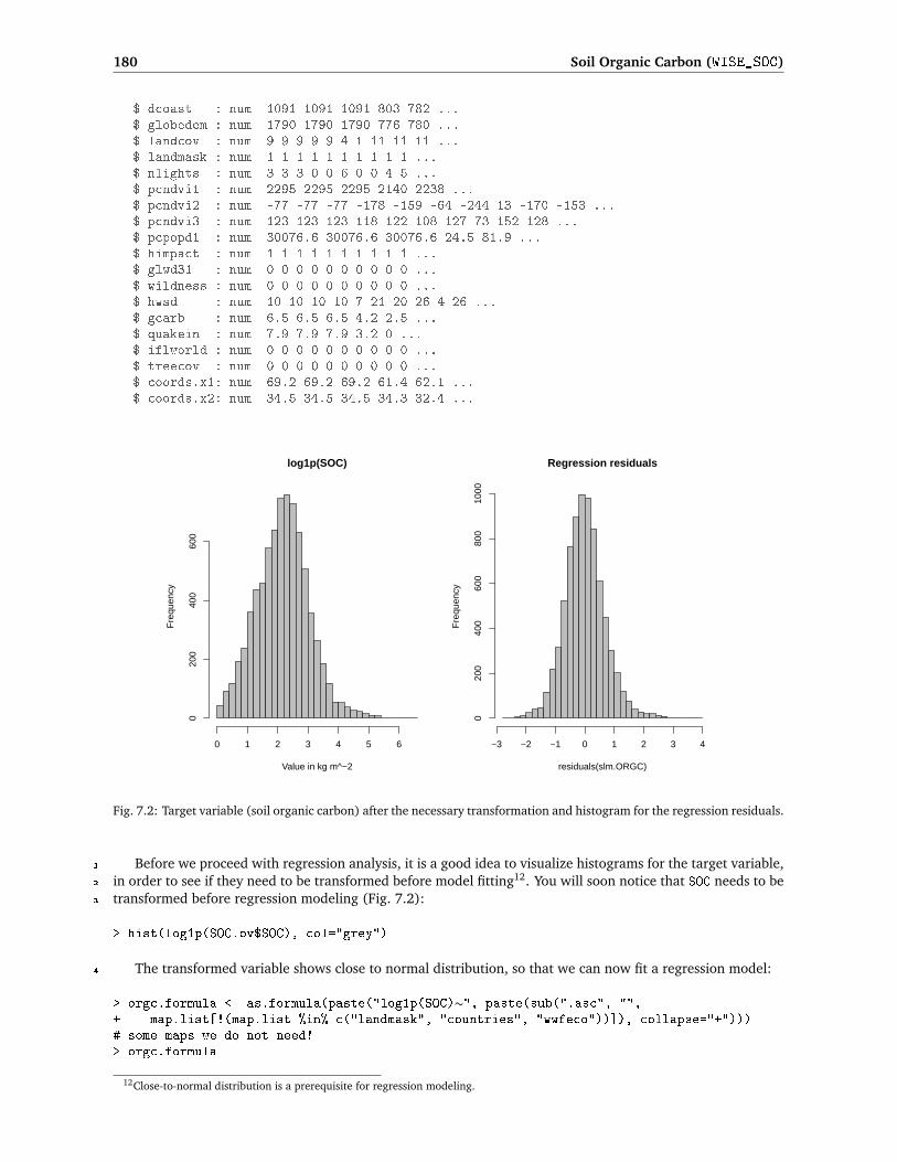
180 Soil Organic Carbon (WISE_SOC)
$ dcoast : num 1091 1091 1091 803 782 ...$ globedem : num 1790 1790 1790 776 780 ...$ landcov : num 9 9 9 9 9 4 1 11 11 11 ...$ landmask : num 1 1 1 1 1 1 1 1 1 1 ...$ nlights : num 3 3 3 0 0 6 0 0 4 5 ...$ pcndvi1 : num 2295 2295 2295 2140 2238 ...$ pcndvi2 : num -77 -77 -77 -178 -159 -64 -244 13 -170 -153 ...$ pcndvi3 : num 123 123 123 118 122 108 127 73 152 128 ...$ pcpopd1 : num 30076.6 30076.6 30076.6 24.5 81.9 ...$ himpact : num 1 1 1 1 1 1 1 1 1 1 ...$ glwd31 : num 0 0 0 0 0 0 0 0 0 0 ...$ wildness : num 0 0 0 0 0 0 0 0 0 0 ...$ hwsd : num 10 10 10 10 7 21 20 26 4 26 ...$ gcarb : num 6.5 6.5 6.5 4.2 2.5 ...$ quakein : num 7.9 7.9 7.9 3.2 0 ...$ iflworld : num 0 0 0 0 0 0 0 0 0 0 ...$ treecov : num 0 0 0 0 0 0 0 0 0 0 ...$ coords.x1: num 69.2 69.2 69.2 61.4 62.1 ...$ coords.x2: num 34.5 34.5 34.5 34.3 32.4 ...
log1p(SOC)
Value in kg m^−2
Fre
quen
cy
0 1 2 3 4 5 6
020
040
060
0
Regression residuals
residuals(slm.ORGC)
Fre
quen
cy
−3 −2 −1 0 1 2 3 4
020
040
060
080
010
00
Fig. 7.2: Target variable (soil organic carbon) after the necessary transformation and histogram for the regression residuals.
Before we proceed with regression analysis, it is a good idea to visualize histograms for the target variable,1
in order to see if they need to be transformed before model fitting12. You will soon notice that SOC needs to be2
transformed before regression modeling (Fig. 7.2):3
> hist(log1p(SOC.ov$SOC), col="grey")
The transformed variable shows close to normal distribution, so that we can now fit a regression model:4
> orgc.formula <- as.formula(paste("log1p(SOC)∼", paste(sub(".asc", "",+ map.list[!(map.list %in% c("landmask", "countries", "wwfeco"))]), collapse="+")))# some maps we do not need!> orgc.formula
12Close-to-normal distribution is a prerequisite for regression modeling.

7.3 Regression modeling 181
log1p(SOC) ∼ biocl01 + biocl02 + biocl04 + biocl05 + biocl06 +biocl12 + biocl15 + dcoast + globedem + landcov + nlights +pcndvi1 + pcndvi2 + pcndvi3 + pcpopd1 + himpact + glwd31 +wildness + hwsd + gcarb + quakein + iflworld + treecov
> lm.ORGC <- lm(orgc.formula, SOC.ov@data)> slm.ORGC <- step(lm.ORGC, trace=-1) # step-wise regression> summary(slm.ORGC)$adj.r.squared
[1] 0.363
This shows that the predictors explain 36% of variability in the SOC values (cumulative density of organic 1
carbon in the soil). For Digital Soil Mapping projects (Lagacherie et al., 2006), this is a promising value. 2
For practical reasons (computational intensity), we will further focus on using only the top 20 most signif- 3
icant predictors to generate predictions. These can be selected by using: 4
> pr.rank <- rank(summary(slm.ORGC)$coefficients[,4])<20> SOC.predictors <- attr(summary(slm.ORGC)$coefficients[pr.rank,1], "names")[-1]> SOC.predictors
[1] "biocl01" "biocl02" "biocl04" "biocl12"[5] "globedem" "landcov9" "landcov12" "nlights"[9] "glwd312" "glwd314" "glwd317" "hwsd4"[13] "hwsd6" "hwsd17" "hwsd19" "hwsd25"[17] "hwsd26" "quakein"
After we have determined the top 20 most significant predictors, we can make predictions by using the 5
SAGA multiple linear regression module. However, before we can produce predictions in SAGA, we need 6
to prepare the indicator maps and a shapefile with transformed target variable. For example, to prepare 7
indicators for different classes of land cover, we can use: 8
> for(j in c("9","12")){> worldmaps$tmp <- ifelse(worldmaps$landcov==j, 1, 0)> write.asciigrid(worldmaps["tmp"], paste("landcov", j, ".asc", sep=""), na.value=-1)> }...# list all indicators and convert to SAGA grids:> indicator.grids <- c(list.files(getwd(), pattern="hwsd[[:digit:]]*.asc",+ recursive=F, full=F),+ list.files(getwd(), pattern="glwd31[[:digit:]]*.asc", recursive=F, full=F),+ list.files(getwd(), pattern="landcov[[:digit:]]*.asc", recursive=F, full=F))> rsaga.esri.to.sgrd(in.grids=indicator.grids,+ out.sgrds=set.file.extension(indicator.grids, ".sgrd"), in.path=getwd())
We also need to prepare the point map with transformed target variables: 9
> SOC.ov$SOC.T <- log1p(SOC.ov$SOC)> SOC.ov$HOTH.T <- sqrt(SOC.ov$HOTH)> writeOGR(SOC.ov[c("SOC.T","HOTH.T")], "SOC_ov.shp", "SOC_ov", "ESRI Shapefile")
which now allows us to use SAGA GIS to make predictions using multiple linear regression: 10
> rsaga.geoprocessor(lib="geostatistics_grid", module=4,+ param=list(GRIDS=paste(set.file.extension(SOC.predictors, ".sgrd"), collapse=";"),+ SHAPES="SOC_ov.shp", ATTRIBUTE=0, TABLE="regout.dbf", RESIDUAL="res_SOC.shp",+ REGRESSION="SOC_reg.sgrd", INTERPOL=0))
...1: R² = 15.508441% [15.508441%] -> biocl02
2: R² = 21.699108% [6.190666%] -> globedem

182 Soil Organic Carbon (WISE_SOC)
3: R² = 24.552229% [2.853121%] -> hwsd4
4: R² = 26.552463% [2.000235%] -> biocl12
5: R² = 30.908089% [4.355626%] -> biocl01
6: R² = 31.498327% [0.590238%] -> hwsd26
7: R² = 31.993559% [0.495233%] -> hwsd6
8: R² = 32.407088% [0.413529%] -> hwsd17
9: R² = 32.738160% [0.331072%] -> landcov12
10: R² = 33.136920% [0.398761%] -> landcov9
11: R² = 33.434208% [0.297288%] -> hwsd19
12: R² = 33.700079% [0.265871%] -> biocl04
...
which shows that the best predictors are Mean Diurnal Range (biocl02), elevation (globedem), various1
soil types (hwsd), annual temperature (biocl01), temperature seasonality (biocl04), annual precipitation2
(biocl12), and land cover classes. Most of variation in SOC values can be explained by using only bioclimatic3
maps.4
The resulting map (Fig. 7.3) shows that high organic carbon concentration in soil can be mainly observed5
in the wet and cooler areas (mountain chains); deserts and areas of low biomass have distinctly lower soil6
organic carbon. Surprisingly, the model predicts high SOC concentration also in arctic zones (Greenland) and7
Himalayas, which is an obvious artifact. Recall that the sampling locations have not been chosen to represent8
all possible environmental conditions, so the model is probably extrapolating in these areas (see also p.59).9
To speed up further analysis we will focus on estimating SOC for South American continent only. This is the10
continent with best (most consistent) spatial coverage, as visible from Fig. 7.3 (below). For further analysis,11
we do not really need all maps, but just the estimate of the trend (SOC_reg). We can reproject the maps using12
(see also §6.5):13
> SA.aea <- "+proj=aea +lat_1=-5 +lat_2=-42 +lat_0=-32 +lon_0=-60 +x_0=0 +y_0=0+ +ellps=aust_SA +units=m +no_defs"> rsaga.geoprocessor(lib="pj_proj4", 2,+ param=list(SOURCE_PROJ="\"+proj=longlat +datum=WGS84\"",+ TARGET_PROJ=paste('"', SA.aea ,'"', sep=""), SOURCE="SOC_reg.sgrd",+ TARGET="m_SOC_reg.sgrd", TARGET_TYPE=2, INTERPOLATION=1,+ GET_SYSTEM_SYSTEM_NX=586, GET_SYSTEM_SYSTEM_NY=770, GET_SYSTEM_SYSTEM_X=-2927000,+ GET_SYSTEM_SYSTEM_Y=-2597000, GET_SYSTEM_SYSTEM_D=10000))
SAGA CMD 2.0.4
library path: C:/PROGRA∼2/R/R-29∼1.2/library/RSAGA/saga_vc/moduleslibrary name: pj_proj4module name : Proj.4 (Command Line Arguments, Grid)author : O. Conrad (c) 2004-8
Load grid: SOC_reg.sgrd...ready
Parameters
Inverse: noSource Projection Parameters: +proj=longlat +datum=WGS84Target Projection Parameters: +proj=aea +lat_1=-5 +lat_2=-42 +lat_0=-32+lon_0=-60 +units=m +no_defs +x_0=0 +y_0=0 +ellps=aust_SA

7.3 Regression modeling 183
3.20
2.70
2.20
1.70
5.0
3.3
1.7
0.0
log1p(kg / m^2)
ISRIC WISE profile density
predicted Soil Organic Carbon
Fig. 7.3: Predicted values of the target variable (log1p(SOC)) using the 20 most significant predictors and multiple linearregression module in SAGA GIS (above). ISRIC WISE coverage map — sampling density on 0.5 arcdegree grid derivedusing kernel smoothing (below).
Grid system: 0.1; 3600x 1300y; -179.95x -64.95ySource: SOC_regTarget: [not set]Shapes: [not set]X Coordinates: [not set]Y Coordinates: [not set]Create X/Y Grids: noTarget: grid systemInterpolation: Bilinear Interpolation
Source: +proj=longlat +datum=WGS84
Target: +proj=aea +lat_1=-5 +lat_2=-42 +lat_0=-32 +lon_0=-60 +x_0=0+y_0=0 +ellps=aust_SA +units=m +no_defs
Save grid: m_SOC_reg.sgrd...ready
> gridsSA <- readGDAL("m_SOC_reg.asc")
m_SOC_reg.asc has GDAL driver AAIGridand has 770 rows and 586 columns

184 Soil Organic Carbon (WISE_SOC)
> names(gridsSA) <- "SOC_reg"> proj4string(gridsSA) <- CRS(SA.aea)> SA.bbox <- gridsSA@bbox> SA.bbox
min maxx -2932000 2928000y -2602000 5098000
which will reproject and resample the predicted log1p(SOC) map from geographic coordinates to the Albers1
Equal-Area Conic projection system13, commonly used to represent the whole South American continent.2
7.4 Modeling spatial auto-correlation3
We have explained some 36% of variation in the SOC values using worldmaps. Next we can look at the4
variograms i.e. try to improve interpolations using kriging. Because we focus only on the South American5
continent, we also need to subset the point map of profiles:6
# reproject the profile data:> GSPD.aea <- spTransform(GSPD, CRS(SA.aea))> writeOGR(GSPD.aea, "GSPD_aea.shp", ".", "ESRI Shapefile")# subset the points:> rsaga.geoprocessor(lib="shapes_tools", module=14,+ param=list(SHAPES="GSPD_aea.shp", CUT="m_GSPD_aea.shp",+ METHOD=0, TARGET=0, CUT_AX=SA.bbox[1,1], CUT_BX=SA.bbox[1,2],+ CUT_AY=SA.bbox[2,1], CUT_BY=SA.bbox[2,2]))
which will subset the input point map to 1729 points. These can be now analyzed for spatial auto-correlation:7
> m_SOC <- readShapePoints("m_GSPD_aea.shp", CRS(SA.aea))> m_SOC.ov <- overlay(gridsSA, m_SOC)> m_SOC.ov$SOC <- m_SOC$SOC> m_SOC.ov <- remove.duplicates(m_SOC.ov) # many duplicate points!> sel <- !is.na(m_SOC.ov$SOC)&!is.na(m_SOC.ov$SOC_reg)> res_SOC.svar <- variogram(log1p(SOC) ∼ SOC_reg, m_SOC.ov[sel,])> SOC.rvgm <- fit.variogram(res_SOC.svar, vgm(nugget=var(SOC.ov$SOC, na.rm=T)/2,+ model="Exp", range=80000, sill=var(SOC.ov$SOC, na.rm=T)/2))> SOC.rvgm
model psill range1 Nug 0.3879486 0.02 Exp 0.1151655 823650.5
which shows that the residuals are correlated up to the distance of >1000 km. This number seems unrealistic.8
In practice, we know that soils form mainly at watershed level or even at short distances, so chances that9
two profile locations that are so far away still make influence on each other are low. On the other hand, from10
statistical perspective, there is no reason not to utilize this auto-correlation to improve the existing predictions.11
Variograms for the original variable and regression residuals can be seen in Fig. 7.4. Note also that the12
variance of the residuals is about 70% of the original variance, which corresponds to the R-square estimated13
by the regression model. Compare also this plot to some previous exercises, e.g. Fig. 5.8. We can in general14
say that the nugget variation of SOC is relatively high, which indicates that our estimate of global SOC will be15
of limited accuracy.16
7.5 Adjusting final predictions using empirical maps17
Once we have estimated the variogram for residuals, we can proceed with regression-kriging14:18
13http://spatialreference.org/ref/esri/102033/14In this case implemented as kriging with external drift, and with a single predictor — regression estimate (see §2.1.4).

7.5 Adjusting final predictions using empirical maps 185
Original variable
distance
sem
ivar
ianc
e
0.1
0.2
0.3
0.4
0.5
0.6
500000 1000000 2000000 3000000
+
++
+ + ++ + + + + +
+ + +
14490
2962037868
451175283958057613256521166648700447022470212
678726408259725
Residuals
distance
sem
ivar
ianc
e
0.1
0.2
0.3
0.4
0.5
0.6
500000 1000000 2000000 3000000
++ + + + + + +
+ + + ++ +
+
Fig. 7.4: Variograms for SOC fitted in gstat using standard settings.
# block regression-kriging:> m_SOC.rk <- krige(log1p(SOC) ∼ SOC_reg, m_SOC.ov[sel,], gridsSA, SOC.rvgm,+ nmin=30, nmax=40, block=c(10e3, 10e3))
[using universal kriging]Warning message:In points2grid(points, tolerance, round, fuzz.tol) :
grid has empty column/rows in dimension 2
# back-transform values:> m_SOC.rk$SOC_rk <- expm1(m_SOC.rk$var1.pred)
in this case, gstat reported about empty pixels in the map that have been removed. The final regression-kriging 1
map of SOC for South American continent can be seen in Fig. 7.5. The RK model predicts even in the areas 2
where there are almost no soil profiles, hence the map is possibly of poor quality in some regions. To improve 3
this map, we can use the USDA–produced Soil Organic Carbon Map15, which is shown in Fig. 7.5 (2): 4
# reproject and import the USDA map:> download.file("http://spatial-analyst.net/worldmaps/SOC.zip",+ destfile=paste(getwd(), "/SOC.zip", sep=""))> unzip("SOC.zip")# resample to the same grid:> rsaga.esri.to.sgrd(in.grids="SOC.asc", out.sgrd="SOC.sgrd", in.path=getwd())> rsaga.geoprocessor(lib="pj_proj4", 2,+ param=list(SOURCE_PROJ="\"+proj=longlat +datum=WGS84\"",+ TARGET_PROJ=paste('"', SA.aea ,'"', sep=""),+ SOURCE="SOC.sgrd", TARGET="m_SOC_USDA.sgrd", TARGET_TYPE=2, INTERPOLATION=1,+ GET_SYSTEM_SYSTEM_NX=m_SOC.rk@[email protected][[1]],+ GET_SYSTEM_SYSTEM_NY=m_SOC.rk@[email protected][[2]],+ GET_SYSTEM_SYSTEM_X=m_SOC.rk@[email protected][[1]],+ GET_SYSTEM_SYSTEM_Y=m_SOC.rk@[email protected][[2]],+ GET_SYSTEM_SYSTEM_D=10000))> rsaga.sgrd.to.esri(in.sgrds="m_SOC_USDA.sgrd", out.grids="m_SOC_USDA.asc",+ out.path=getwd(), prec=3)> m_SOC.rk$SOC_USDA <- readGDAL("m_SOC_USDA.asc")$band1
15http://soils.usda.gov/use/worldsoils/mapindex/

186 Soil Organic Carbon (WISE_SOC)
Recall from §2.1.3 that, if we know the uncertainty of both maps, we can derive a weighted average and1
create a combined prediction. In this case, we do not have any estimate of the uncertainty of the USDA SOC2
map; we only have an estimate of the uncertainty of RK SOC map. Because there are only two maps, the3
weights for the RK map (Fig. 7.5 (3)) can be derived using the inverse of the relative prediction variance (see4
p.25); the remaining weights for the USDA map can be derived as 1−w. Or in R syntax:5
# merge the two maps (BCSP formula):> w <- sqrt(m_SOC.rk$var1.var)/sqrt(var(log1p(m_SOC.ov$SOC), na.rm=T))> m_SOC.rk$w <- 1-w/max(w, na.rm=TRUE)> m_SOC.rk$SOC.f <- m_SOC.rk$w * m_SOC.rk$SOC_rk + (1-m_SOC.rk$w) * m_SOC.rk$SOC_USDA
25
18
12
5
25
18
12
5
0.850
0.767
0.683
0.600
25
18
12
5
ISRIC WISE USGS corrected map
kg / m^2kg / m^2 kg / m^2
correction
(1) (2) (3) (4)
Fig. 7.5: Soil Organic Carbon stock (kg C m−2) for South America: (1) predicted using regression-kriging, (2) the USDASOC map produced using soil regions; (3) sampling locations and map of weights derived as the inverse relative predictionerror; (4) the final corrected map of SOC derived as a weighted average between the maps (1) and (2).
The final corrected map of SOC is shown in Fig. 7.5 (4). In this case, the USDA map is assume to be more6
spatially ‘consistent’ about the actual SOC stock. The weighted average between the two maps is possibly the7
best estimate of the Soil Organic Carbon given the limited data. To validate this map, one would need to8
collect block estimates of SOC with a support size of 10 km (Heuvelink and Pebesma, 1999).9
7.6 Summary points10
Estimation of organic carbon stock using ISRIC WISE profiles and geostatistical techniques is possible, but the11
final map is of limited quality: (a) soil samples are fairly clustered (Fig. 7.3, below), for many regions there12
are still no measured soil data; (b) predictors used are rather coarse (cca. 10 km), which limits the regression13
modeling; (c) the residuals for SOC consequently show high nugget. The map presented in Fig. 7.5 (1) can14
be considered to be especially poor where the density of point samples is low. The question remains whether15
the models would improve if one would consider fitting variogram models locally (moving window), or by16
using finer-grain predictors (<10 km) that could potentially be able to explain short-range variation. On the17
other hand, we know that there is inherent uncertainty in the geo-locations of WISE profiles, so that not even18
finer-grain predictors would help us improve the predictions.19
If you repeat a similar analysis with other soil variables of interest, you will notice that the gridded predic-20
tors explain only between 10–40% of the observed variability in the values (e.g. 36% for SOC, 11% for HOTH,21
22% for SAND, 28% for SILT, 15% for CLAY), which means that these maps are of limited accuracy. The var-22
iograms also show relatively high nugget, which also means that about 30–60% of variability in these target23
variables cannot be explained by regression-kriging. This is particulary problematic for large regions that are24
completely under represented — most of the former Russian federation, Australia and Canada (see the map in25
Fig. 7.1). Nevertheless, the main patterns of soil parameters produced using ISRIC WISE will often correspond26
to our empirical knowledge: high soil organic carbon mainly reflects the cold and wet temperatures (Batjes,27
1996); deep soils are predicted in the tropical regions and areas of high biomass (Eswaran et al., 1993);28
texture classes are connected with the land cover, relief and soil mapping units etc.29

7.6 Summary points 187
The advantage of automating the operations, on the other hand, is that these maps can be easily updated 1
once the ISRIC WISE becomes more representative and of higher quality. Due to the data processing automa- 2
tion, many other important soil parameters from the ISRIC WISE database could easily be revised once updates 3
with better geographical coverage are released . 4
Self-study exercises: 5
(1.) Estimate nugget variation for SOC for the five largest countries in the world. Plot the variograms one 6
over the other. 7
(2.) Compare the Global Biomass Carbon Map distributed by The Carbon Dioxide Information Analysis Cen- 8
ter and the total soil carbon map shown in Fig. 7.5(4). Are the two maps correlated and how much? 9
Where is the difference highest and why? 10
(3.) Repeat the spatial prediction of soil carbon by focusing on the North American continent (HINT: resam- 11
ple the maps following the previous exercise in §6.5.) 12
(4.) Which country in the world has highest reserves of organic carbon in absolute terms (total soil carbon 13
in tones), and which one in relative terms (average density of carbon)? 14
(5.) Compare spatial prediction of SOC for South America and Africa (regression-kriging variance). Why are 15
soil profile data in South America more suited for geostatistical mapping? 16
(6.) Interpolate soil textures (SAND, SILT, CLAY) using the same procedure explained in the text and produce 17
global maps. 18
(7.) Focus on Australia and compare the soil organic carbon map available from the Australian soil atlas with 19
the map shown in Fig. 7.3. Plot the two maps next to each other using the same grid settings. 20
Further reading: 21
Æ Batjes, N.H., 2009. Harmonized soil profile data for applications at global and continental scales: up- 22
dates to the WISE database. Soil Use and Management 25, 124-127. 23
Æ Lagacherie, P., McBratney, A.B., Voltz, M., (eds) 2006. Digital Soil Mapping: An Introductory Perspec- 24
tive. Developments in Soil Science, Volume 31. Elsevier, Amsterdam, 350 p. 25
Æ Ruesch, A., Gibbs, H.K., 2008. New IPCC Tier-1 Global Biomass Carbon Map For the Year 2000. Carbon 26
Dioxide Information Analysis Center, Oak Ridge National Laboratory, Oak Ridge, Tennessee, 45 p. 27
Æ http://www.isric.org — ISRIC World Soil Information center; 28
Æ http://www.pedometrics.org — The international research group on pedometrics; 29
Æ http://www.globalsoilmap.net — International consortium that aims to make a new digital soil 30
map of the world using state-of-the-art and emerging technologies for soil mapping and predicting soil 31
properties at fine resolution; 32

188 Soil Organic Carbon (WISE_SOC)

8 1
Species’ occurrence records (bei) 2
8.1 Introduction 3
A special group of Species Distribution Models (SDMs) focuses on the so-called occurrence-only records — 4
pure records of locations where a species occurred (Tsoar et al., 2007). Although such point data set can be 5
considered of interest to geostatistics, standard geostatistical techniques cannot be used to generate (realized) 6
species’ distributions using occurrence-only data, mainly for two reasons: (1) absence locations are missing 7
(‘1’s only), so that it is not possible to analyze the data using e.g. indicator geostatistics; and (2) the sampling 8
is purposive and points are often clustered in both geographical and feature spaces, which typically causes 9
difficulties during the model estimation. 10
Spatial statisticians (e.g. Diggle (2003); Bivand et al. (2008)) generally believe that geostatistical tech- 11
niques are suited only for modeling of features that are inherently continuous (spatial fields); discrete objects 12
(points, lines, polygons) should be analyzed using point pattern analysis and similar methods. This exercises 13
tries to bridge this gap. It demonstrates how to combine geostatistical techniques with conceptually different 14
techniques — point pattern analysis and Niche analysis — to allow prediction of species’ distributions using 15
regression-kriging. For more info about the theoretical basis for this approach see section 2.6. This chapter is 16
based on an article published in Ecological Modeling journal (Hengl et al., 2009b). 17
We will use the data set bei, distributed together with the spatstat1 package, and used in school books 18
on point pattern analysis by Baddeley (2008) and many other authors. This data set consists of a point map 19
showing observed locations of trees of the species Beilschmiedia pendula Lauraceae. This is only a small part 20
of the Barro Colorado Island 50 Hectare Plot2 Data set (Panama) that contains about 2 million records — 21
complete inventory of all plant species and numerous plant and environmental attributes for six time periods 22
(Leigh et al., 2004). 23
8.1.1 Preparation of maps 24
To run the bei.R script, you will first need to load the following packages: 25
> library(spatstat)> library(adehabitat)> library(gstat)> library(splancs)> library(rgdal)> library(RSAGA)
We load the bei data set directly from R: 26
1http://spatstat.org2http://www.stri.org/english/research/facilities/terrestrial/barro_colorado/
189

190 Species’ occurrence records (bei)
> data(bei)> str(bei)
List of 5$ window :List of 5..$ type : chr "rectangle"..$ xrange: num [1:2] 0 1000..$ yrange: num [1:2] 0 500..$ units :List of 3.. ..$ singular : chr "metre".. ..$ plural : chr "metres".. ..$ multiplier: num 1.. ..- attr(*, "class")= chr "units"..$ area : num 5e+05..- attr(*, "class")= chr "owin"$ n : int 3604$ x : num [1:3604] 11.7 998.9 980.1 986.5 944.1 ...$ y : num [1:3604] 151 430 434 426 415 ...$ markformat: chr "none"- attr(*, "class")= chr "ppp"
Fig. 8.1: The bei data set — locations of Beilschmiedia pendula Lauraceae trees, and a 5 m DEM used as environmentalpredictor. Viewed from south to north.
This shows locations of individual trees (a total of 3604 trees) observed in a 1000 m by 500 m rectangular1
window3. The beginning of the rectangle is at Lat. 9.15125°, Long. -79.8553°. The bei object is of type ppp,2
which is the native spatstat format (point pattern data set in the two-dimensional plane). If you would try to3
analyze this data set using some geostatistical package, you would soon find out that not much can be done4
because this is not even a binary variable.5
8.1.2 Auxiliary maps6
In addition to the point map a map of elevation and slope gradient is provided in the bea.extra data set:7
> str(bei.extra, max.level=1)
List of 4$ elev :List of 11..- attr(*, "class")= chr "im"$ grad :List of 11..- attr(*, "class")= chr "im"
3What makes this data set especially suitable for this exercise is the fact that the complete population of the trees has been mapped forthe area of interest.

8.2 Species distribution modeling 191
We can extend the initial list of covariates and attach two more maps that we can derive in SAGA and then 1
import back into R — the wetness index and vertical distance from the channel network (Fig. 8.2): 2
> grids <- as(bei.extra[[1]], "SpatialGridDataFrame")> names(grids)[1] <- "elev"> grids$grad <- as(bei.extra[[2]], "SpatialGridDataFrame")$v> write.asciigrid(grids["elev"], "dem.asc")> write.asciigrid(grids["grad"], "grad.asc")# Generate the wetness index and vertical distance from the channel network:> rsaga.esri.to.sgrd(in.grids="dem.asc", out.sgrds="dem.sgrd", in.path=getwd())# Filter the spurious sinks:> rsaga.geoprocessor(lib="ta_preprocessor", module=2,+ param=list(DEM="dem.sgrd", RESULT="dem_f.sgrd"))> rsaga.geoprocessor(lib="ta_hydrology", module=15, param=list(DEM="dem_f.sgrd",+ C="catharea.sgrd", GN="catchslope.sgrd", CS="modcatharea.sgrd", SB="twi.sgrd", T=10))> rsaga.geoprocessor(lib="ta_channels", module=0, param=list(ELEVATION="dem.sgrd",+ CHNLNTWRK="chnlntwrk.sgrd", CHNLROUTE="channel_route.sgrd", SHAPES="channels.shp",+ INIT_GRID="dem_f.sgrd", DIV_CELLS=10, MINLEN=30))> rsaga.geoprocessor(lib="ta_channels", module=3, param=list(ELEVATION="dem.sgrd",+ CHANNELS="chnlntwrk.sgrd", ALTITUDE="achan.sgrd", THRESHOLD=0.1, NOUNDERGROUND=TRUE))> rsaga.sgrd.to.esri(in.sgrds=c("twi.sgrd","achan.sgrd"),+ out.grids=c("twi.asc","achan.asc"), prec=1, out.path=getwd())> grids$achan <- readGDAL("achan.asc")$band1> grids$twi <- readGDAL("twi.asc")$band1
Fig. 8.2: Auxiliary (environmental) maps used to explain species’ distribution: Elevation (elev), Slope in % (grad),Topographic Wetness Index (twi) and Altitude above channel network in m (achan) derived in SAGA GIS.
where twi.sgrd is the Topographic Wetness Index, and achan.sgrd is the Altitude above channel network. 3
For more info about the SAGA syntax, see section 3.1.2 or refer to Conrad (2007). 4
We will now implement all steps described in §2.6 to predict the spatial density of trees over the area of 5
interest (M=20301 grid nodes). To test our algorithm we will use a 20% sub-sample of the original population 6
and then validate the accuracy of our technique versus the whole population. 7

192 Species’ occurrence records (bei)
8.2 Species distribution modeling1
8.2.1 Kernel density estimation2
We start by estimating a suitable bandwidth size for kernel density estimation (Eq.2.6.3). For this we use the3
method of Berman and Diggle (1989), as described in Bivand et al. (2008, p.166–167), that looks for the4
smallest Mean Square Error (MSE) of a kernel estimator:5
> gridbbox <- as.points(list(x=c(grids@bbox[1,1], grids@bbox[1,2], grids@bbox[1,2],+ grids@bbox[1,1]), y=c(grids@bbox[2,1], grids@bbox[2,1], grids@bbox[2,2], grids@bbox[2,2])))> mserw <- mse2d(as.points(coordinates(bei.pnt)), gridbbox, 100, 10*bei.pixsize)> bw <- mserw$h[which.min(mserw$mse)]> plot(mserw$h,mserw$mse, type="l")
0 20 40 60 80 100 120
−5
05
1015
mserw$h
mse
rw$m
se
Fig. 8.3: Selection of the optimal bandwidth using the method of Berman and Diggle (1989).
This shows that the optimal bandwidth size is about 4 m. But since our grid cell size is 5 m this bandwidth6
is not really suited for this scale of work. Based on the plot from above we only know that we should not use a7
bandwidth finer/smaller than 5 m; coarser bandwidths are all plausible. We can also consider the least squares8
cross validation method to select the bandwidth size using the method of Worton (1995), as implemented in9
the adehabitat package:10
> bei.pnt <- data.frame(x=bei$x, y=bei$y, no=rep(1, length(bei$x)))> coordinates(bei.pnt) <- ∼ x+y> dem.asc <- import.asc("dem.asc")> bei.kdens <- kernelUD(xy=as.data.frame(bei.pnt@coords), id=NULL, h="LSCV", grid=dem.asc)
Warning message:In kernelUD(xy = as.data.frame(bei.pnt@coords), id = NULL, h = "LSCV", :The algorithm did not converge within the specified range of hlim: try to increase it
This does not converge either4, hence we need to set the bandwidth size using some ad hoc method. As a11
rule of thumb we can start by estimating the smallest suitable range as the average size of block:12
p =p
area(BHR)/N (8.2.1)
13
and then set the bandwidth size at two times this value. There are 3605 trees (N) in the area of size14
507,525 m2, which means that we could use a bandwidth of 24 m (H):15
4This is unfortunately a very common problem with many real point patterns.

8.2 Species distribution modeling 193
> bei.pixsize <- sqrt(areaSpatialGrid(grids)/length(bei$x))> bei.pixsize
[1] 11.86687
We next derive a relative kernel density map using the standard methods in the spatstat package (Eq.2.6.7). 1
The resulting density map is shown in Fig. 8.4: 2
> bei.ppp <- ppp(coordinates(bei.pnt)[,1], coordinates(bei.pnt)[,2],+ marks=bei.pnt$no, window=as(grids[1], "owin"))# reformat the point pattern so it fits the grids:> summary(bei.ppp)
Marked planar point pattern: 3604 pointsAverage intensity 0.0071 points per square unitmarks are numeric, of type 'double'Summary:
Min. 1st Qu. Median Mean 3rd Qu. Max.1 1 1 1 1 1
Window: binary image mask101 x 201 pixel array (ny, nx)pixel size: 5 by 5 unitsenclosing rectangle: [-2.5, 1002.5] x [-2.5, 502.5] unitsWindow area = 507525 square units
> bei.dens <- density(bei.ppp, sigma=2*bei.pixsize)> grids$dens <- as(bei.dens, "SpatialGridDataFrame")$v# relative density:> grids$densr <- grids$dens/(max(grids$dens, na.rm=T))> bei.pnt.plot <- list("sp.points", bei.pnt, pch="+", cex=.7, col="black")> plt.dens1 <- spplot(grids["densr"], scales=list(draw=F), at=seq(0,1,0.025),+ col.regions=grey(rev(seq(0,1,0.025))), sp.layout=bei.pnt.plot)
Fig. 8.4: Relative intensity estimated for the original bei data set (left), and its 20% sub-sample (right). In both cases thesame bandwidth was used: H=24 m.
If we randomly subset the original occurrence locations and then re-calculate the relative densities, we 3
notice that the spatial pattern of the two maps does not differ significantly, and neither do their histograms: 4
# Randomly subset points:> sel <- runif(length(bei.pnt$no))<0.2> bei.sub.pnt <- bei.pnt[sel,]> bei.sub <- ppp(coordinates(bei.sub.pnt)[,1], coordinates(bei.sub.pnt)[,2],+ marks=bei.sub.pnt$no, window=as(grids[1], "owin"))# plot(bei.sub)# Derive kernel density:

194 Species’ occurrence records (bei)
> bei.sub.dens <- density(bei.sub, sigma=2*bei.pixsize)> grids$sub.dens <- as(bei.sub.dens, "SpatialGridDataFrame")$v> grids$sub.densr <- grids$sub.dens/(max(grids$sub.dens, na.rm=T))# Plot the second map:> bei.sub.pnt.plot <- list("sp.points", bei.sub.pnt, pch="+", cex=.7, col="black")> plt.dens2 <- spplot(grids["sub.densr"], scales=list(draw=F), at=seq(0,1,0.025),+ col.regions=grey(rev(seq(0,1,0.025))), sp.layout=bei.sub.pnt.plot)> print(plt.dens1, split=c(1,1,1,2), more=T)> print(plt.dens2, split=c(1,2,1,2), more=T)
then check if the two maps follow the same distribution:1
> t.test(grids$sub.densr, grids$densr)> t.test(grids$sub.densr, grids$densr)
Welch Two Sample t-test
data: grids$sub.densr and grids$densrt = -6.5351, df = 40567.5, p-value= 6.432e-11alternative hypothesis: true difference in means is not equal to 095 percent confidence interval:-0.010186940 -0.005486209sample estimates:mean of x mean of y0.1125212 0.1203578
which confirms that the two maps basically follow the same distribution. This supports our assumption that2
the relative density map (Eq.2.6.7) can be indeed reproduced also from a representative sample (n=721).3
We proceed with preparing the environmental predictors and testing their correlation with the density val-4
ues. We can extend the original single auxiliary map (DEM) by adding some hydrological parameters: slope, to-5
pographic wetness index and altitude above channel network. We want to attach the SpatialGridDataFrame6
class maps to the original im class bei.extra, which means that we need to ‘coerce’ the objects to format of7
interest:8
> bei.extra$twi <- as.im(as.image.SpatialGridDataFrame(grids["twi"]))> bei.extra$achan <- as.im(as.image.SpatialGridDataFrame(grids["achan"]))> plot.im(bei.extra, col=grey(rev(seq(0,1,0.025))))
which will produce the map shown in Fig. 8.2. The result of fitting a non-stationary point process with a9
log-linear density using the ppm method of spatstat shows that density is negatively correlated with wetness10
index, and positively correlated with all other predictors (Baddeley, 2008):11
> bei.sub.ppm <- ppm(bei.sub, ∼ elev+grad+twi+achan, covariates=list(elev=bei.extra$elev,+ grad=bei.extra$grad, twi=bei.extra$twi, achan=bei.extra$achan))> summary(bei.sub.ppm)
Point process modelfitted by maximum pseudolikelihood (Berman-Turner approximation)Call:ppm(Q = bei.sub, trend = ∼ elev + grad + twi + achan,covariates = list(elev = bei.extra$elev,...Edge correction: "border"----------------------------------------------------FITTED MODEL:
Nonstationary Poisson process
---- Intensity: ----
Trend formula: ∼ elev + grad + twi + achanModel involves external covariates

8.2 Species distribution modeling 195
Fitted coefficients for trend formula:(Intercept) elev grad twi achan-9.00309481 0.01675857 4.24494406 -0.07240637 0.03017035
We can actually use this model to predict the species density by using the generic predict method: 1
> bei.ppm.trend <- predict(bei.sub.ppm, type="trend", ngrid=c(grids@[email protected][2],+ grids@[email protected][1]), window=as(grids[1], "owin"))> plot(bei.ppm.trend)> plot(bei.sub, add=T, pch=".")
Fig. 8.5: Trend model "ppm" predicted using elevation, slope, topographic wetness index and altitude above channelnetwork as environmental covariates (left); Habitat Suitability Index (0-100%) derived in the adehabitat package usingthe same list of covariates (right).
Visually (Fig. 8.5), we can see that the predicted trend seriously misses some hot-spots i.e. clusters of points. 2
It seems that using point pattern analysis techniques to map (realized) species’ distribution with covariates is 3
of limited use. A comparison between the Akaike Information Criterion (AIC) for a model without predictors 4
and with predictors shows that there is a slight gain in using the covariates to predict the spatial density: 5
> fitnull <- ppm(bei.sub, ∼ 1)> AIC(fitnull)
[1] 10496.56
> AIC(bei.sub.ppm) # this is a slightly better model
[1] 10289.79
Just for a comparison, we can also fit a GLM model5 using all grid nodes: 6
> bei.ppp.lm <- glm(sub.densr ∼ grad+elev+twi+achan, grids@data, family=poisson())
There were 50 or more warnings (use warnings() to see the first 50)
> summary(bei.ppp.lm)
This shows a similar picture: the best predictor of the density is TWI. 7
5We need to use the log as the link function because the density values are heavily skewed.

196 Species’ occurrence records (bei)
8.2.2 Environmental Niche analysis1
We proceed with the Environmental Niche Factor Analysis (Hirzel and Guisan, 2002), as implemented in the2
adehabitat6 package (Calenge, 2007). Our objective is to derive the Habitat Suitability Index (0–100%) which3
basically shows potential spreading of a species in the feature space (environmental preference). We need to4
prepare the maps in the adehabitat native format:5
> beidata <- data2enfa(as.kasc(list(dem=import.asc("dem.asc"), grad=import.asc("grad.asc"),+ twi=import.asc("twi.asc"), achan=import.asc("achan.asc"))), bei.sub.pnt@coords)# run ENFA and make predictions of habitat suitability index:> enfa.bei <- enfa(dudi.pca(beidata$tab, scannf=FALSE), beidata$pr, scannf=FALSE, nf=2)
Warning message:In predict.enfa(enfa.bei, beidata$index, beidata$attr) :the enfa is not mathematically optimal for prediction:please consider the madifa instead
> bei.dist <- predict(enfa.bei, beidata$index, beidata$attr)> grids$bei.dist <- as.SpatialGridDataFrame.im(asc2im(bei.dist))$v# Convert to 0-100 scale:> sum.dist <- summary(grids$bei.dist)> grids$rankv <- rank(grids$bei.dist, ties.method="first")> grids$hsit <- ifelse(grids$bei.dist<sum.dist[["Median"]],+ (1-grids$rankv/max(grids$rankv))*100, (1-grids$rankv/max(grids$rankv))*100)> grids$hsi <- 100*round((grids$hsit-min(grids$hsit, na.rm=T))/(max(grids$hsit,+ na.rm=T)-min(grids$hsit, na.rm=T)), 3)> plt.HSI <- spplot(grids["hsi"], at=seq(0,100,2.5), col.regions=bpy.colors())
The resulting HSI map shows that this species generally avoids the areas of high wetness index, i.e. it6
prefers ridges/dry positions (Fig. 8.5, right). This spatial pattern is now more distinct (compare with the trend7
model in Fig. 8.5, left). This demonstrates the power of ENFA, which is in this case more suited for analysis of8
the occurrence-only locations than regression analysis and/or the point pattern analysis.9
8.2.3 Simulation of pseudo-absences10
In the next section we will use the results of Niche analysis to generate pseudo-absences. Recall (§2.6) that11
insertion of pseudo-absences is an important step because it will allow us to fit regression models. We use12
two maps as weight maps to randomize allocation of the pseudo-absences: the geographical distance from the13
occurrence locations and habitat suitability index. We first derive the buffer distance to the points in SAGA14
GIS:15
# first the buffer distance:> rsaga.geoprocessor(lib="grid_gridding", module=3, param=list(GRID="bei_buffer.sgrd",+ INPUT="bei_sub.shp", FIELD=0, LINE_TYPE=0, USER_CELL_SIZE=grids@grid@cellsize[[1]],+ USER_X_EXTENT_MIN=grids@bbox[1,1]+grids@grid@cellsize[[1]]/2,+ USER_X_EXTENT_MAX=grids@bbox[1,2]-grids@grid@cellsize[[1]]/2,+ USER_Y_EXTENT_MIN=grids@bbox[2,1]+grids@grid@cellsize[[1]]/2,+ USER_Y_EXTENT_MAX=grids@bbox[2,2]-grids@grid@cellsize[[1]]/2))# now extract a buffer distance map and load it back into R:# (the parameters DIST and IVAL are estimated based on the grid properties)> rsaga.geoprocessor(lib="grid_tools", module=10, param=list(SOURCE="bei_buffer.sgrd",+ DISTANCE="bei_dist.sgrd", ALLOC="bei_alloc.sgrd", BUFFER="bei_bdist.sgrd",+ DIST=sqrt(areaSpatialGrid(grids))/3, IVAL=grids@grid@cellsize[[1]]))> rsaga.sgrd.to.esri(in.sgrds="bei_dist.sgrd", out.grids="bei_dist.asc",+ out.path=getwd(), prec=1)> grids$buffer <- readGDAL("bei_dist.asc")$band1# relative distance:> grids$bufferr <- grids$buffer/max(grids$buffer, na.rm=T)
6http://cran.r-project.org/web/packages/adehabitat/

8.2 Species distribution modeling 197
By combining HSI and buffer map around the occurrence locations (Eq.2.6.11) we can generate the same 1
amount of pseudo-absence locations: 2
# weight map:> grids$weight <- ((100*grids$bufferr+(100-grids$hsi))/2)^2> dens.weight <- as.im(as.image.SpatialGridDataFrame(grids["weight"]))> bei.absences <- rpoint(length(bei.sub.pnt$no), f=dens.weight)> bei.absences <- data.frame(x=bei.absences$x, y=bei.absences$y,+ no=rep(0, length(bei.sub.pnt$no)))> coordinates(bei.absences) <- ∼ x+y# combine the occurences and absences:> bei.all <- rbind(bei.sub.pnt["no"], bei.absences["no"])
One realization of the simulated pseudo-absences (overlaid over the weight map) can be seen in Fig. 8.10a. 3
Correct insertion of pseudo-absences is crucial for the success of regression analysis (see Chefaoui and Lobo 4
(2008) for discussion), hence it also a good idea to visually validate each simulated pseudo-absence and 5
remove ‘suspicious’ candidates. 6
8.2.4 Regression analysis and variogram modeling 7
Before we run any regression analysis we will convert the original four predictors to principal components (in 8
order to reduce their dimensions and the multicolinearity effect): 9
# derive PCs from the original predictors:> pc.grids <- prcomp( ∼ grad+elev+twi+achan, scale=TRUE, grids)> pc.comps <- as.data.frame(pc.grids$x)> pointgrids <- as(grids, "SpatialPointsDataFrame")> pc.comps$X <- coordinates(pointgrids)[,1]> pc.comps$Y <- coordinates(pointgrids)[,2]> coordinates(pc.comps) <- ∼ X+Y> gridded(pc.comps) <- TRUE> pc.comps <- as(pc.comps, "SpatialGridDataFrame")> spplot(pc.comps, c("PC1","PC2","PC3","PC4"),+ col.regions=grey(c(rep(0,10),seq(0,1,0.05),rep(1,10))), cuts=40)
Fig. 8.6: Principal Components generated using the original predictors.

198 Species’ occurrence records (bei)
●● ●
●
●●
●●
● ● ● ●●
●
●
●
●● ●
●
●
●●
●
●
●
●
●
●
●
●●●
●●
●
●
●●
●
●●●●
● ●●
●
●●●●●
●
●
●● ●
●●●
●●●
●●●
●
●
●●
●●
●● ●●●
●●
● ●●● ●
●●●
●●
●● ●●
●●●
●
●●●● ●●●
●●●
●●
●
●
●●
●
●●
●●
●●●
●
●
●●●●
●●
●
●●●●●●
●
●
●●
●
●●●●
●●●
●
●●
●
●
●● ●●
●●●
●●●
●
●
●●
●●
●●
●
●
● ●●●
●●
●
●
●
●
●
●●
●
●
●
●●
●●●●
●
●● ●
●●●
●
●
●●●●● ●
●●● ●
●
●
●
●●●● ●
●●
●
●
●●
● ●
●
●●●
●●
●●●
●
●
●
●
●
●
●●
● ●
● ●●●● ●●●●
●
●
●●
●●●
●
●●●●
●●●●●
●
●●
●●
●
●●●
●●●
●
●●
●
●
●
●
●●
●●●●
●●
●●
●
●
●
●●
●●●
●●
●●●●
●●
●
●
●● ●
●●
●
●●
●●● ●
●
●●
● ●
●●●
●●●●●
●
●●●●●●
●
●●●
●●
●●●
●
●
●●●●
●●●
● ●●●●
●
● ●● ● ●●
● ●●
●● ●●
●
●
●
●
● ●●
●●● ●● ●●●
●●
●●●●
●●●●
●●●● ●● ●●
●●●
●●●●●
●
●●●
● ●●
●
●● ●
●
●
●●
●●
● ●
●● ● ● ●●
●●●●
●
●●
●
●●
●
●
●
●
●
●●●●
●
●●
●●
●
●●●●●
●
●●
●●
●
●●●
●●
●
●
●
●
●●
●
●● ●
● ●
●
●
●●
●●
●●
●
●●
●
●●●
●●
●
●
●●
● ●●●
●
●●
●
●
●
●
●
●● ●●
●
●● ● ●
●
●
●
● ●
●●●●
●●
●●
●●●
●
●●
● ●●●●
●
●
●●
●●
●
●
●
●
●●
●
●
●
● ●
●● ●●● ●●
●●
● ●
●●
●●
●●
●
●
●●
●●
● ●
●●
● ●
●
●●●
●
●●●●
●
●●●
●
●● ●
●
●
●● ●
●●●
●●●
●●
●
● ●
●
●
●
●
●
●
●●
●
●
● ●●
●
●
●
●●
●
●●
●
●●
●
●●
●
●
●●
●●
●●●
●
●●
●
●
●
●
●
●
●
●
●
●
●
●
●●
●
●
●
●
●
●
●
●
●
●
●
●
●
●●
●
●
●
●
●
●
●
●
●●
●
●
●● ●
●●
●
●
●●
●●●
●●
●●
●
●
●
●
●
●
●
●
●
●
●
●
●
●
●
●
●●
●
●
●
●
●
●
●
●
●
●
●
●
●
●
●
●●
●
●
●
●
●
●
●
●●
●
●
●
●●
●
●
●
●
●●
●
●
●
●●
●
●
●
●
●
●●
●
●
●
●
●
●
●
●
●●
●
●
●
●●
●
●●
●
●
●
●
●
●
●
●
●
●
●
●
●
●
●
●●
●
●
●
●
●
●
●
●●
●
●
●
●
●
●
●
●
●
●●
●
●●
●●
●
●
●
●
●
●
●
●
●
●
●
●
●
●
●
●
●
●●
●
●
●
●
●
●
●
●●
●
●
●
●
●
●
●
●
●
●
●
●
●
●
●
●
●●
●
●
●
●
●
●
●
●
●
●
●
●
●
●
●
●
●
●
●
●
●
●●
●
●
●
●
●
●
●●
●
●
●
●
●
●
●
●
●
●
●
●
●
●
●●
●
●
●
●
●
●
●
●
●
●
●
● ●
●
●
●
●
●
●
●
●
●
●
● ●
●
●●
●
●
●
●
●
● ●
●
●
●
●
●●
●
●
●
●
●●
●
●
●
●
●
●
●
●
●
●
●
●
●●
●
●●
●
●
●
●
●
●
●
●
●
●
●
●
●
●
●●
●
●
●
● ● ●
●
●
●
●
●
●
●
●
●
●
●●
●
●
●
●
●
●
●
●
●
●●
●
●
●
●
●
●●
●
●
●
●
●
●
●
●
●●
●
●
●
●
●
●
●
●
●
●
●
●
●
●
●
●
●
●
●
●
●
●
●
●
●
●
●
●
●
●
●
●
●
●
●
●●
●
●
●
●
●
●●●
●
●
●
●●●
●
●
●
●
●
●
●
●
●
●
●
●
●
●
●
●
●
●
●
●
●
●
●
●
●
●
●
●
● ●
● ●
●
●
●
●
●
●●●
●
●
●●
●
●
●
●
●
●
●●
●
●
●
●●●
●
● ● ●
●
●
●
●
●
●
●
●
●
●
●
●
●
●
●
●
●
●
●
●●
●
●
●●
●
●
●
●
●
●
●
●●
●
●
● ●
●
●
●
●
●●
●
●
●
●
●
●
●
●
●
●
●●
●
●
●
●
●
●
●
●
●
●
●●
●
●
●
●
●●
●
●
●
●
●
●●
●
●
●
●●
●
●
●
●
●●
●
●
●●●
●
●
●
●●
●
●
●
●
●
●
●
●
●
●
● ●●
●
●
●
●
●
●
●
●
●
●
●
●
●
●
●
●●
●
●
●
●●●
●
●
●
●
●
●
●
●
●
●●
●
●●
●
●
●
●
●
●
●
●
●
●
●
●
●
●
●
●
●
●
●
●
●
−4 −2 0 2
−6
−4
−2
02
4
PC1
logi
t(de
nsity
)●
● ●
●
●●
●●
●● ● ●●
●
●
●
●● ●●
●
●●
●
●
●
●
●
●
●
●●●
●●
●
●
●●
●
●●●●
●●●
●
●●●●●
●
●
●●●
●●●
●●●●●
●
●
●
●●
● ●
●●●●●
●●
●●●● ●
●●●
●●
●●●●
●●●
●
●● ●●●● ●
●●●
●●
●
●
●●
●
●●●●
●●●
●
●
●●●●
●●
●
●●
●●●●
●
●
●●
●
●●●●
●●●
●
●●
●
●
●●●●
●●●
●●●
●
●
●●
●●
●●
●
●
●●●●
●●
●
●
●
●
●
● ●
●
●
●
●●●
● ●●
●
●●●
●●●
●
●
●●●●●●
●●●●
●
●
●
●● ●●●
●●
●
●
●●●●
●
●●●
●●
●●●
●
●
●
●
●
●
●●
●●
● ● ●●● ● ●●●
●
●
●●
●●●
●
●●●●●●●●
●
●
●●
●●
●
●●●
●●●
●
●●
●
●
●
●
●●
● ●●●
●●
●●
●
●
●
●●
●●●
●●
●●●●
●●
●
●
●●●●
●●
●●
●●● ●
●
●●
● ●
●●●
●●●●●
●
●●●●●●
●
●●●
●●
●●●
●
●
●●●●
● ●●
●●●●●
●
● ●●● ●●
● ●●
●● ●●
●
●
●●
● ●●
●● ●●●●●
●●
●
●●●●
●●●●
●●● ● ●● ●●
●●●
●●●●●
●
●●●
● ●●
●
●●●●
●
●●
●●
●●
●●● ● ●●
●●●●
●
●●
●
●●
●
●
●
●
●●●●
●
●
●●
●●
●
●●●●●
●●●
●●
●
●●●
●●
●
●
●
●
●●
●
●●●
●●
●
●
●●
●●
●●
●
● ●
●
●●●
●●
●
●
●●
●●●●
●
●●
●
●
●
●
●
●● ●●
●
●● ● ●
●
●
●
● ●
●●●●
● ●●
●
●●●
●
●●
●●●●●
●
●
●●
●●
●
●
●
●
● ●
●●
●
●●
●● ●●● ●●
● ●
●●
●●
●●
●●
●
●
●●
●●
●●
●●
● ●
●
●●●
●
●● ●●
●
●●●
●
●●●
●
●
● ●●
●● ●●
●●●●
●
● ●
●
●
●
●
●
●
●●
●
●
●● ●
●
●
●
●●
●
●●
●
●●
●
●●
●
●
●●
●●
●●●
●
●●
●
●
●
●
●
●
●
●
●
●
●
●
●●
●
●
●
●
●
●
●
●
●
●
●
●
●
●●
●
●
●
●
●
●
●
●
●●
●
●
●● ●
●●
●
●
●●
●●●
●●
●●
●
●
●
●
●
●
●
●
●
●
●
●
●
●
●
●
●●
●
●
●
●
●
●
●
●
●
●
●
●
●
●
●
●●
●
●
●
●
●
●
●
●●
●
●
●
●●
●
●
●
●
●●
●
●
●
●●
●●
●
●
●
●●
●
●
●
●
●
●
●
●
●●
●
●
●
● ●
●
●●
●
●
●
●
●
●
●
●
●
●
●
●
●
●
●
●●
●
●
●
●
●
●
●
●●
●
●
●
●
●
●
●
●
●
●●
●
●●
●●
●
●
●
●
●
●
●
●
●
●
●
●
●
●
●
●
●
● ●
●
●
●
●
●
●
●
●●
●
●
●
●
●
●
●
●
●
●
●
●
●
●
●
●
●●
●
●
●
●
●
●
●
●
●
●
●
●
●
●
●
●
●
●
●
●
●
● ●
●
●
●
●
●
●
●●
●
●
●
●
●
●
●
●
●
●
●
●
●
●
●●
●
●
●
●
●
●
●
●
●
●
●
● ●
●
●
●
●
●
●
●
●
●
●
● ●
●
●●
●
●
●
●
●
●●
●
●
●
●
●●
●
●
●
●
●●
●
●
●
●
●●
●
●
●
●
●
●
●●
●
● ●
●
●
●
●
●
●
●
●
●
●
●
●
●
●
●●
●
●
●
● ● ●
●
●
●
●
●
●
●
●
●
●
●●
●
●
●
●
●
●
●
●
●
●●
●
●
●
●
●
● ●
●
●
●
●
●
●
●
●
●●
●
●
●
●
●
●
●
●
●
●
●
●
●
●
●
●
●
●
●
●
●
●
●
●
●
●
●
●
●
●
●
●
●
●
●
●●
●
●
●
●
●
●● ●
●
●
●
● ●●
●
●
●
●
●
●
●
●
●
●
●
●
●
●
●
●
●
●
●
●
●
●
●
●
●
●
●
●
● ●
● ●
●
●
●
●
●
●● ●
●
●
●●
●
●
●
●
●
●
●●
●
●
●
●●●
●
●●●
●
●
●
●
●
●
●
●
●
●
●
●
●
●
●
●
●
●
●
●●
●
●
●●
●
●
●
●
●
●
●
●●
●
●
● ●
●
●
●
●
●●
●
●
●
●
●
●
●
●
●
●
●●
●
●
●
●
●
●
●
●
●
●
●●
●
●
●
●
●●
●
●
●
●
●
●●
●
●
●
●●
●
●
●
●
●●
●
●
●●●
●
●
●● ●
●
●
●
●●
●
●
●
●
●
●●●
●
●
●
●
●
●
●
●
●
●
●
●
●
●
●
●●
●
●
●
●●
●
●
●
●
●
●
●
●
●
●
● ●
●
●●
●
●
●
●
●
●
●
●
●
●
●
●
●
●
●
●
●
●
●
●
●
−2 −1 0 1 2 3 4
−8
−6
−4
−2
02
4
PC2
logi
t(de
nsity
)
Fig. 8.7: Correlation plot PC1/PC2 versus the logit-transformed density.
which shows that the first component reflects pattern in the twi and grad; the third component reflects1
pattern in achan (Fig. 8.6). Next, we can overlay the predictors and the estimated intensities at occurrence2
and absence locations:3
> bei.ov2 <- overlay(pc.comps, bei.all)> bei.ov2$no <- bei.all$no# convert the original values to logits:> bei.ov2$log.densr <- log((bei.ov2$densr+0.001)/(1-(bei.ov2$densr-0.001)))> summary(bei.ov2$log.densr)
Min. 1st Qu. Median Mean 3rd Qu. Max.-6.908 -3.378 -1.882 -2.297 -1.197 4.253
> var(bei.ov2$log.densr, na.rm=T)
[1] 3.666165
The benefit of converting the target variable to logits and the predictors to PCs is that the relationship4
between the two is now close to linear (Fig. 8.7):5
> scatter.smooth(bei.ov2$PC1, bei.ov2$log.densr, span=19/20, col="grey",+ xlab="PC1", ylab="logit(density)")> lm3.bei <- lm(log.densr ∼ PC1+PC2+PC3+PC4, bei.ov2@data)> summary(lm3.bei)
Call:lm(formula = log.densr ∼ PC1 + PC2 + PC3 + PC4, data = bei.ov2@data)
Residuals:Min 1Q Median 3Q Max
-4.09463 -0.98535 0.04709 0.99504 5.52267
Coefficients:Estimate Std. Error t value
(Intercept) -2.35896 0.04247 -55.546PC1 -0.40174 0.02864 -14.025PC2 -0.79147 0.03684 -21.482PC3 -0.34820 0.04629 -7.522PC4 0.34360 0.07423 4.629

8.2 Species distribution modeling 199
Pr(>|t|)(Intercept) < 2e-16 ***PC1 < 2e-16 ***PC2 < 2e-16 ***PC3 9.65e-14 ***PC4 4.02e-06 ***---Signif. codes: 0 '***' 0.001 '**' 0.01 '*' 0.05 '.' 0.1 ' ' 1
Residual standard error: 1.559 on 1379 degrees of freedomMultiple R-squared: 0.3441, Adjusted R-squared: 0.3422F-statistic: 180.9 on 4 and 1379 DF, p-value: < 2.2e-16# the model explains 34% of variation
●
● ●●
● ●● ●●
●
●●
●
●●
● ●●
●
●● ●●●●●
●●●
●
●●
● ●●
●●● ●● ● ●● ●●●●●
●●●●
● ●
●
●●
●●●●
●● ●●
●● ●●
●● ●●
●
●●
●●
●
●●● ●
●● ●● ●●●●
●●
●●●●●●●
●●●
●● ●●
●
●●
●
●●
●
●
●
●●
●
●●
●
●
● ●
●
●●
●
●
●
●
●●●
●●●
●
●
●● ●
●●●
●
● ●●
●
●●
●●
●●
●●
●
●
●●
●
●●
●
●
●
●●
●
●
●● ●
●
●
●
●
●
●●●●
●●●●
●●●
● ●●●●
●●
●
●
● ●● ●● ●●●● ●●●
●●●● ●
●●●
●●● ●
●● ●●●● ●●
● ●● ●●
● ●●●● ●
●●● ●
●●
●●
●●●● ●●
●●●●● ●
●●● ●●●
●●●● ●●
●●●●
●●●
●
●●●●●●●●
●●
● ●
●
●
●
● ●● ●●●● ●● ●● ● ● ●● ●●
●●●
●●
● ●● ●●●●●●●● ●●
●●
●
●●
●●●
●
● ● ●●●●●
●● ● ●● ●●● ●●
● ●●●●● ●● ●●● ●● ● ●●● ● ● ●
●●● ●●●●● ●●● ●
●●
●
●●● ●
● ● ●●●●●●●
● ● ●● ●●
● ●● ●●● ●●
●
●
●● ●
●●
●
●●●●●●
● ●●● ● ●●●● ●● ●●● ●● ●●●
●●●
●
● ●●●
●●●●●
●●
●●●● ●●●●
●● ●●
●●●●●●●●●●●●
●
●●
●●●●● ●●● ● ●● ●●
●●
●
●●
● ●
●●●●
●
●●●●● ●
●●● ●
●
●●●
●●●
●
●
●●●●●
●●●●
● ●●● ● ● ●
●
●●
●●
●●●●
●
●●●●●
●● ●●
●●●
●●●●●
●
●● ● ●●●●●●
● ●●
●●
●●●
●●●
●
●●
●●●
●●●●
●
●●●●
●●
●●●
●
●
●
●
●
●●● ●●
● ●
●●
●●
●●
● ●●●●●●●
●●
●
● ●●●●●● ● ●●● ●
●
●
●●●●
● ● ●●
●
●
●
●●
● ●
●
●
●●●●●●
● ●●
●●●●●●
●●●●●●
●●
● ●
●
●
●●●●●
●●●
●
●
●
●●
●●●
● ●● ●● ●
●● ●●●
● ●●●●
●●
●
●●● ●●
●
●● ●● ●
●●
●●● ●●●●
●●● ●● ● ●●●●● ●
●●
●
●
●●●
●●
●●●●●
●●
●●
●●●●● ●
●
● ●●●●●
●●●
●●●●● ●●●●●
●●●
●●
●
●●● ●
●
●●
●
●●●● ●●
●●●●
●●
●●●
●
●●
●
●
●
●●●
●
●●
●●●●●●● ●●
● ●
●
●●
● ●●●
●●● ●●
●●●
●● ●● ●●●●
●●●●
●●
●
●
●
● ●
●
●●●●●● ●●●● ●
●●●
●●
●●
●●●
●●
●
●●●●●●
●● ●●●●●●
●
●●●
●●
●● ●
●●●●
●
●●
● ●● ●●● ●● ● ●● ●●
●
●● ●
●
●● ●●●
●
●●
●
●
● ●●●● ●● ●●●●
● ●
●
●
●
●
●●●● ●● ●●
●●●●●●●● ●●● ●●
●
●●
● ●●●●
● ●●
●
●
●●●●●●●●
● ●●● ●●
●
●●● ●●●
● ●●
●
●●●●●
●●●●●● ●●●●
●●●●●
● ●●●●● ●
●● ●
● ●●● ●●
●●
● ●
● ●●●●●●● ●●
●●●●●●●●
●●●●●●●
●
●● ●● ●●
●● ●
●●
●●
●●●
●●
● ●●
●
●
●●●●
●
●● ●●●
●●●●●
● ●●●
● ●●●● ●●● ●●●●
●
● ●●●
●●
●
●●
●●● ●●●
●
●●
●●●
●
●●●
●●●●● ●● ●●●● ●
●
●
●
●
●
●
●
●
●●●●●
●●
●
●
●
●
●
●
●
●
●
●●
●
●
●●●● ●
● ●● ●● ●●●●
●●
●●
●●●●
●●● ●●●●
●●●
●● ● ●●●●● ●
●●●●●●
●●
●●●●
●●
●●
●
●●
● ●●●
●●●●●●
●●●●
●●
●●
●
●
●
●
●●
●
●●●●
●●
●●●●●●●●●●●
●●●●●
● ●
●
●
●● ●●● ●●● ●●●●
● ●●●
●●●●●
●●●●
●
● ●●● ●● ●●●
●●●●●
●●●●●
●●
●●
●
●
●
●●
●●●●
●●●●●●●●●●●
●
●
●
●
●●●●●
●●●●●●●●
●●●●●●●●●●●●●●●●●
●
●●●●●
●●
●
●
●
●
●●●●●●●
●
●
●●●
●
●●
●●
●●●●
●●●
● ●●
●●●
●
●
●●
●
●●
●
●●●
●●
●
●
●●
●●
●●●
●
●● ●●
●● ●
● ●
●●●●
●
●●●●
●● ●
●●●●●
●●
● ●●● ●●
●
●●
●●●
●
●
●●
●
●●●
●
●
●
●
●
●● ●● ● ● ●●
●●●
● ●
●●●
●●
●●●●●●
●
●
●●
●●●
●
●●
●
●
●● ●
●●●●● ●● ●● ●●●● ●●
●● ●●●●
●●●●
●●
● ●●
●
●●●●
●● ●●
●●●
● ●●●
●● ●●●● ●●
●●● ●●●
●●
●●●
●●●
●●
●
● ●● ●●●●
●
●● ●
● ●●● ●●
●●●
● ●●
●●
●●●●
●●● ●●●●●
●●
●●●
●●
●●
●●●
●●●● ●● ● ●
●●
●
●●●●● ●
● ●●●● ●●●
●●●●● ●●●●
●●●● ●●● ●●
●●●●●● ●●
●●
●
●●●●●● ●● ●
●●●● ●●●
●●
●●
●●
●●●●
●●●●
●● ● ●●●● ●●●●●●●●●●●●● ●
●●
●
●● ●
●●●
●●●●
●●
●● ●●● ●
●●●●● ●
● ●
●●●
●●●
●
●●●● ● ●●● ●●●●●
●●● ●●●●
●●●●
●
●● ●● ● ●
● ●
●●●●●● ●●●
●●●●● ●●●●
●●● ●●● ● ● ●● ●●
●●●●●●
● ●●
● ● ●●
●●●●
●●●●● ●● ● ●●●●● ●●●● ●● ●●●●●●●●●●●●●●●●●●
●●●
●●●●● ● ●
●●●●●
● ● ●●●●● ●●● ● ● ●
●
●●●
● ●● ●●
●●●
●●●●● ●● ● ●● ● ●●●●●●
●● ●●●●●●●● ●●● ●●
● ●● ●●●
● ●●● ●
●●● ●●●
●●● ●● ●
●●
●●
●
●●
●
●
●●
●●●
●
●●●
● ● ●● ●●● ●●●●●
●●●●
●●●●●●●●●●●● ●●● ● ● ●●●
●●●●●●●●●●●●● ●● ●
●●●
●●
●●
●●
●
●●●●●●●●●● ● ●●● ●●
●●●●
●●
●
●
●●●●● ●●●●● ●
●●●
●● ●●
● ●●●● ●●
●●●
●
●
●● ●
●●
●●●
●●●
● ●
●●●●●●●● ● ●●●●●●● ●●
●●
●● ●●
●● ●●●● ●●
●●● ●● ●●● ● ●● ● ●●●
●
●●
●●●
●●●●
●●● ●
●●
●● ●●●
●
●●
●
●
●●
●●●●●
●
●●●●
●●● ●● ●●
●
●●●
●
●●
● ●●
●●●●
●
●●●
●●●● ●● ●● ●● ●● ●●
●● ●●
●
●
●●●
●● ●●
●●● ●●
●●
●●
● ●●
●
● ●●
●●
●●●
●● ●
●
● ●
● ●
●●
●●
●●
●●
●
●
●●
●●
●
●●●
●●
●
●●●
●●
● ●
●●
●●●
●●
●●
●●●
●● ●
●●
●●● ●
● ●
●
●● ● ● ●●
●
●
●●
●●
●
●● ●
●●●●
●
● ● ●●
●●
●
●●●●●●● ● ●
● ● ●●●●●
●
●●●● ●●●●●
●●
●
●●●
●●
●
●●●●
●●●
●●
●
●●
●●
●
●
● ●●
●●●●●●●
●
●●
●
●
●
●●
●●
●●
●●
●
●
●
●
●●●
●●
●●
●
●●
●
●●●●●●●
●
●
●
●●
●●●●●
●
●●●●●●
●●●
●●●●
●●●
●●
●●
●
●●
●
●
●
●
●●●●●●●
●
●●
●●●●
●●●●●
●
●●●
●●●●
●
●
●●●●
●●
●
● ●
●
●
●●
●● ●
●● ●
●●●
●
●●
●
● ●
● ●●
●●
●
●
●●
●●●
●●
●
●● ●
●
●
● ●
●●●●●●●
●●● ●
●
●
●
●●●
●
●
● ●●●
●
●●
●●●
●●
●
●●
●●●●
● ●●
● ● ●
●
●
●● ●●
●●●●●
●
●
●
●
● ●
●
●●
●●●
●●
● ●●
●●
●●
●
●
●
●
●
●
●
●
●●●
●
●
●●●
●
●
●
●
●● ● ●●●●
●●●●
●
●●●●●●
●●●●
●●● ●
●
●
●
●
●
●●●
●
● ●●
●
●●●●
● ●
●
●
●●
● ●
●
●●
●●●
●
●
●
●
●●
●●●
● ●●●●●●●●
●●●
●●
●●● ●
●
●●
●●
●●
● ●
●
●
●●●
●●● ●
●
●●●● ●●
●●
● ● ●●●
● ●
●● ●
●●
● ●●
●● ●●●
●●●●
●●
●●
●
●●●
●
●●●●●
●
●
●●●●
●
●
●●
●●
●
●
●●●
●
●●●●
●●●● ●●
● ●
●●
●
●
●●●
●
●●●
●
● ●●
●
●
●
●●●
●●
●
●● ●
●●●●
●
●
●
●●●●
●
●
●●●● ●
●
●
● ●●
● ●
●●●
●
●
● ●●●●●
●
●●●
●●
●
●
●●
●
●
●
●●●●●●
●●
● ●●
●
●
●
●●
●
●
●
●
●●
●
●
●
●
●
●
●●
●●●●
●
●
●
●● ●●● ●●
●
●
●
●●●●
●
●●
●
●●●
●●
●
●
●
●
●
●●
●●
● ●●
●
●
●●
●
●●● ●
●
●●●● ●
●●●●
●
● ●●
●●
●
●●●
●
●●
●
●
●●
●
●●
●●●●●●●
●●●●
●
●
●●
●
●●
●●
●● ●
●●
●
●
●●●
●
●●●
●● ●●●
●
●
● ●
●●
●
●
●
●●
●●
●
●●
● ●●
●
●
●
●
● ●
●●●
●
●● ●
●
●●●
●●●●●
●●●●●●
●
●
●
●
●●●
● ● ●
●
●● ●●● ●● ●
●●●
●
●
●●●●
●●●●
● ●
●●●
●
●●●
●●●●●● ●●●●●●●● ●●
●
●
● ●●
● ●
●
●●●
●●
●
● ●● ●●●
●
●
●
●
●●●●●●
●
●●● ●
●●● ● ● ●●
●● ●
●● ●● ●
●
●
●
● ●●
●●
●
●
●
●●●
●
●
●
●
●●
●●
●
●●●
●●
●●●
●
●
●
●●●
●●
●●
● ●● ●●● ●●
●
● ●●●
●●
●
●
●●
●
●●
●●
●●
●
●●
●●
●●●
●●●
●
●●
●
●
●
●●●
●
●
●
●
●
●
●
●●
●
●
●
●●
●
●
●
●
●●
●
●●
●●
●
●●
●●
●
●●
●
●
●
●●●
●●●
●●
●
●
●
●
●
●
●
●●
●
●● ●
●●
●●
●
●
●
●
●●
●
●
● ●
●
●●● ●
●
●
●
●
●
●● ●
●
● ●
● ●
●
●
●●●
●
●
●●
●
●●●
● ●
●
●●
●
●●● ●
●
●●
●
●
●
●
●● ●●●
● ●
●
●●●●●●
●● ●●
●●
● ●●●
●●●
●●●● ●●
● ●● ●●
0 20 40 60 80 100
0.0
0.2
0.4
0.6
0.8
1.0
HSI
dens
ity (
occu
rren
ces)
●
●
●●
●
● ●●
●
●●
●●●
● ●● ● ●
●
●
●●
● ●●●
● ●● ●●●● ●
●●
●
●●
●
●
●
●
●
●
●
●●
●
●
●● ●
●
●●
●
●
●
● ●
●
●
●●
●
●
●● ● ●●
●
●●
●●
● ●●●●
● ●●●●● ●
●●
●●●
●●
●●●
●●●●● ●●●
●●
●
●● ●
●●
●●●● ●● ●
● ●
●
●●●●● ●●●● ●
● ● ●●●
●●
●
●●● ●● ●
●●●
●
●●●
●
●
●●●● ●●
●
●
●●●
●●
●
●●
●
●●
●●●●
● ●
●●●
●
●
●●●
●
●●
●
●●
●●●
●
● ●●● ●●
●
●
●●
●
● ●●●
●●●●
●
●●●
●
●
●●
●● ●●
●
●
●●● ●● ●●
●●
●
●●●●●
●
●
●●
●
●
●●
●
● ●●
●
● ●
● ●
● ●●
●
●●●
●
●
● ●
●
●●
●●
●●
●●
●●●
●●
●●
●
●●● ●
●●●
●
●●
●●●
● ●●
●●
●
●
●●●●●●
●●●
● ●●●●
●●
● ●
● ●●
●
●● ●●
●●
●●●
●
●● ●●●●●●
●●
●
●● ●
●
●
●●
●● ●●
●
●
●
●
●
●
●
●
●● ●●●
●
●●
●●
●
● ●●● ●●
●●
● ●●
●
●●●
●●
●
● ●●
● ●
●●●
● ●● ●●
●●
●●
●
●
●●
●●
●
●●
●●●●●●●
●●●●●●
●
●
●
●
●
●●
●
●
●
●
●●
●
● ●
●
●●●●●
●●●
●●
●●
●
● ●
●
●
●●●
●
●● ●
●●
●●
●
●
●
● ●●●
● ●●
●●●
●●
●●●●
●●
●
●● ●●
●●
●●● ●●
●
●● ●●●
●● ●●●
●●●
●●●● ●
●
●●● ● ● ●●●●
●
●●●
●●
●
●
● ● ●●●● ●
●
●
● ●
●●●●●
●●●
●●●●●
●
● ●●●● ●●●
●●●
●
●
●●● ● ●
●●●
● ●●
● ●● ●●●
●●●●● ●
●●
● ●●●
●●●
●●●●
●●●●●●● ●●
●●●
●
●
●●●
●●●
●● ●●
●
●●●●
●●●●●●● ● ● ●●
●●
●
●
●●●
●
●●● ●
●●
● ●●●●
●●
●● ●
●
●
●
●
● ●●●
●
●
●●
●
●
●
●●
●● ●
● ●
●
●
●
●●●
●
●●
●●
●●
● ● ●
●
●●
●
●●●
●
●
●
●
●
●
●●
●
●●●
●●
●
●●
●●
●●
●
●●●●●
●●
●
●●
●●
●
●●●
●●●
●
●●●
●
●
●
●●
●
●
●●●●
●
●
●
●
●
●
●
●
● ●
●
●
●
●
●
● ●
●
●● ●
●
●
●
●● ●● ●
●●
●
●
●
●
●
●
●●
●●
●●●
● ●●●
● ●
●●
●
●
●
●●
●
●
●●● ● ●
●
●●
●● ●●
●●
●
●
●
●
●
●●
●●
●●
●
●●
●●
●●
●●●
●
●●
●
● ● ●●
●
●
●
●
●
●
●●
●
●
●
●
●●
●
●●●
●●
●
●●
●
● ●●
●●●
● ● ●
●
●●
●●
●
●
●
●●
●
●
●
●
●● ●●●
●
●
●●
●●
●●●
●●
●●
● ●●●
●●●
●
●
●●
●●●
●
●
●
●●
●
●●
● ●
●
●
●●●
●● ●
●
●●
●●
●
●●
●
●●
●
●
●
●
●
●●
●
●
●● ●
●
●
●
●
●
● ●●
●● ●
●●
●
● ●
●
●
●
●
●
●
●
●
●
●
●
●●●
●●●
● ●
●
●●
●●
●●
● ●●
●
●
●
●
●
●
●
●
●● ●●
●
●
●
●●
●
●●
● ●
●
● ●●
●
●●
●●●● ●
●●●
●●
●● ●●
●
● ●
●
● ●●
●
●●
● ●
●
●
●●● ●●●
●● ●
●
●
●●
●
●●
●
●
●●
●●
●
●●● ●
●
●●
●
●
●
●
● ●●●
●
●●●●●
● ●●
●
●●●
●
●● ●
●●
●
●
●
●●
●●
●
●
●
● ●
●
●●
●
●
●
●
●●
●●●
●
●● ●●
●
●
●●
●●
●●
●
●●●●
●
●●
● ●
●
●
●
●
●
● ●●●
●● ● ●
●
●
●
●
●●
●●
●●
●
●● ●
●●
●
●● ●● ●●● ●
●
●
●●
●
●●
●
● ●●● ●●●
●
●
●
●
●
●
●
●●
●
●●●
●
●
● ●●
●
●
●
●
●
●
●●
●●
●
●●
●●
●●
●
●●
●●● ●●
●
●● ●● ●●
●
●
●
●
●●● ●
●
●
●●
●
● ●●
●● ● ●●
●● ●●
●●
●
●
●
●●●
●
●
● ●●
●
●
●●
● ●
● ●
●
●● ●
●
●
●
●
●
● ●●
●
●
●●
●
●●
●
●
●
●
●
●
●
●
●
● ●●
●●
●●
●
●●
●
●
●
●
●
● ●●
●● ●
●
●
●
●
●
●●
●
●
● ●
●
●
●●● ●
●
●●
●●
●
●● ● ●
● ●
●
●
●●
●● ●
●
●
●●
●
●
●
●●
●●● ●●
●
●●
●
●
●
●● ● ●
●
●●
●
●
●
●
●
●●
●
● ●
●●
●
●
●●
● ●●
●
●●
●
●
●
●
●
●●
●
● ●
●
● ●●● ●
●●
● ●
●
●
●●
●
●
●
●
●
●
●
●
●
●
●● ●
●
● ●
●
●
●● ●
●
●●
●
●
●●
●
●●● ●
●
●
●●
●
●
●
●
●
●●
●●
● ●●
●
●
●● ●
●
●
●●
●
●●
●●●
●
●
●●
●
●●
●
●
●● ●
●
●●
●●●
●
●●●
●
●
● ●●
●
●●
●
●
●●
●
●
●●●
●
●
●●
●
●
●
●
●●
● ●
●
●●
●
●
●
●
●
●● ●●
●
●
●
●
●●
●●
●
●
●●
● ●
●
●●
● ●
●
●
●
●
●
●●
●
●
●●
●
●
● ●
●
●
●
●
●
● ●●
●
●●
●
●
●
●
●
●
●
●●
●
●
●
●
●●●
●
●●
●●
●
●●● ●
●
●
●●
●
●
●
●●●
●●
●
●●
●
●
●
●
●
●●
●
●
● ●● ●
●
●● ●
●
● ●●
●
●
●
●●
●●
●●● ●
●
●
●●
●
●
●●
●
●
●
●●● ● ●● ●
●
●
●● ●
●
●●
●● ●
● ●
●●●
●
●● ●●
●● ●●●
●
●●
●
●
●
●
●●
●
● ●●
●
●
●
●
●
●
●
●●
●
●
●
●
●
●
●
●●●●
●
●●
●
●●
●
● ●
●
●● ●
●
● ●●
●
●
● ●●
●●
●● ●
●●
●
●● ●
●●
●
●
●
●
●
● ●●
●
●● ●
●●● ● ●●●
●●
●●
●
●
●●
●
●
●
●●●
●
●●
●
●
●
●
●
●
●
●● ● ●●
●
●●●●
● ●●●
● ●●
●●
●
●
●
●
●● ●
●
●
● ●●
●
●
●
●
●
● ●
● ●
●●
●
●
●
●
●
●
●
●
●
● ●● ●
●
●●
●
●
●
●
●
●● ●●
●
●● ● ●●
●
●●●●
●
●●●●
●●
●
●●●●
●●
●●
●
●
●
●
●
●
●●
●●
●
●●
●
●●
● ●●
●
●
●
●
●● ●● ●●
●●
●
●
●●
●
●
●
●
●
●●
●●
●
●
●
●
●
●
●●
●
●
●
●●
●
●
●● ●
●
●●
●
●
●
●●
●
●● ●●
●
●
●
●●
●●●●
0 20 40 60 80 100
0.0
0.2
0.4
0.6
0.8
1.0
HSI
dens
ity (
occu
rren
ces
+ a
bsen
ces)
HSI (occurrences)
Den
sity
0 20 40 60 80 100
0.00
00.
010
0.02
00.
030
HSI (occurrences + absences)
Den
sity
0 20 40 60 80 100
0.00
00.
005
0.01
00.
015
Fig. 8.8: Correlation plot HSI vs relative density with occurrence-only locations (left) and after the insertion of the pseudo-absence locations (right). Note that the pseudo-absences ensure equal spreading around the feature space (below).
The correlation between the HSI and density is now clearer and the spreading of the points around the HSI 1
feature space is symmetric: 2
# Glue occurrences and pseudo-absences:> bei.all <- rbind(bei.sub.pnt["no"], bei.absences["no"])> scatter.smooth(bei.ov2$hsi[bei.ov2$no>0], bei.ov2$densr[bei.ov2$no>0], span=19/20,+ col="darkgrey", pch=21, cex=.5, xlab="HSI", ylab="density (occurrences-only)")> scatter.smooth(bei.ov2$hsi, bei.ov2$densr, span=19/20, col="darkgrey", pch=21,+ cex=.5, xlab="HSI", ylab="density (+ absences)")> hist(bei.ov2$hsi[bei.ov2$no>0], col="grey", freq=F, breaks=30,+ xlab="HSI (occurrences)", ylab="frequency", main="")> hist(bei.ov2$hsi, col="grey", freq=F, breaks=30,+ xlab="HSI (occurrences + absences)", ylab="frequency", main="")

200 Species’ occurrence records (bei)
Intensity residuals
distance
sem
ivar
ianc
e
0.5
1.0
1.5
2.0
100 200 300
+
+
+
+
++
+
+
+
+ ++
+
+
+
4975
11093
16265
20666
248732749730830
32113
35479
3727638122378133771438101
39113
Binomial GLM residuals
distance
sem
ivar
ianc
e
0.05
0.10
0.15
0.20
100 200 300
+
+
+
+
+
+ +
++
+ + + ++
+
4975
11093
16265
20666
248732749730830
3211335479372763812237813377143810139113
Fig. 8.9: Variogram models for residuals fitted in gstat using occurrence-absence locations: (left) density values (logits),and (right) probability values.
which produces the plot shown in Fig. 8.8 (right). Consequently, the model fitting is more successful: the1
adjusted R-square fitted using the four environmental predictors jumped from 0.07 to 0.34. This demonstrates2
the benefits of inserting the pseudo-absence locations using a feature-space design model. It can be further3
demonstrated that, if we would randomly insert the pseudo-absences, the model would not improve or would4
become even noisier.5
We proceed with analyzing the point data set indicated in Fig. 8.10b using standard geostatistical tools. We6
can fit a variogram for the residuals and then predict relative densities using regression-kriging as implemented7
in the gstat package. For a comparison, we also fit a variogram for the occurrence-absence data but using the8
residuals of the GLM modeling with the logit link function, i.e. using the 0/1 values (Fig. 8.9):9
> glm.bei <- glm(no ∼ PC1+PC2+PC3+PC4, bei.ov2@data, family=binomial())
We can now deal with the residuals by using some standard geostatistical techniques. To fit a variogram10
for the residuals, we run:11
> res.var <- variogram(residuals(lm3.bei) ∼ 1, bei.ov2)> res.vgm <- fit.variogram(res.var, vgm(nugget=0, model="Exp",+ range=sqrt(areaSpatialGrid(grids))/3, psill=var(residuals(lm3.bei), na.rm=T)))> plot(res.var, res.vgm, plot.nu=T, pch="+", main="Intensity residuals")
As with any indicator variable, the variogram of the binomial GLM will show higher nugget and less distinct12
auto-correlation than the variogram for the (continuous) density values (Fig. 8.9). This is also because the13
residuals of the density values will still reflect kernel smoothing, especially if the predictors explain only a14
small part of variation in the density values.15
8.3 Final predictions: regression-kriging16
We can finally generate predictions using a regression-kriging model7:17
# regression part:> vt.gt <- gstat(id=c("dens"), formula=log.densr ∼ PC1+PC2+PC3+PC4, data=bei.ov2)# residuals:> vt.gr <- gstat(id=c("dens"), formula=residuals(lm3.bei) ∼ 1,+ data=bei.ov2, model=res.vgm)> vt.reg <- predict.gstat(vt.gt, pc.comps) # regression part> vt.ok <- predict.gstat(vt.gr, pc.comps, nmax=80, beta=1, BLUE=FALSE,+ debug.level=-1)
7Residuals and the deterministic part are predicted separately.

8.3 Final predictions: regression-kriging 201
# Back-transform:> vt.reg$dens <- exp(vt.reg$dens.pred+vt.ok$dens.pred)/+ (1+exp(vt.reg$dens.pred+vt.ok$dens.pred))> vt.reg$densA <- vt.reg$dens * length(bei.pnt$no)/sum(vt.reg$dens, na.rm=F)> sum(vt.reg$densA) # check if the sum of counts equals the population!
[1] 3604
> bei$n
[1] 3604
To predict the probability of species’ occurrence we run similar steps: 1
> bin.reg <- predict(glm.bei, newdata=pc.comps, type="response", na.action=na.omit)> bin.gr <- gstat(id=c("no"), formula=glm.bei$residual ∼ 1, data=bei.ov2, model=res.bvgm)> bin.ok <- predict.gstat(bin.gr, pc.comps, nmax=80, beta=1, BLUE=FALSE, debug.level=-1)> bin.ok$rk.bin <- bin.reg$fit + bin.ok$no.pred> bin.ok$rk.binf <- ifelse(bin.ok$rk.bin<0, 0, ifelse(bin.ok$rk.bin>1, 1, bin.ok$rk.bin))
The resulting map of density predicted using regression-kriging (shown in Fig. 8.10c) is indeed a hybrid 2
map that reflects kernel smoothing (hot spots) and environmental patterns, thus it is a map richer in content 3
than the pure density map estimated using kernel smoothing only (Figs. 8.4), or the Habitat Suitability Index 4
(Fig. 8.5, right). Note also that, although the GLM-kriging with a binomial link function (Fig. 8.10d) is statisti- 5
cally a more straight forward procedure (it is completely independent from point pattern analysis), its output 6
is limited in content because it also fails to represent some hot-spots. GLM-kriging of 0/1 values in fact only 7
shows the areas where a species’ is likely to occur, without any estimation of how dense will the population 8
be. Another advantage of using the occurrences+absences with attached density values is that we are able not 9
only to generate predictions, but also to generate geostatistical simulations, map the model uncertainty, and 10
run all other common geostatistical analysis steps. 11
1.0
0.7
0.3
0.0
0.80
0.53
0.27
0.00
(a) (b)
(c) (d)
9965
6643
3322
0
1.000
0.667
0.333
0.000
no / grid
[ - ]
relative intensity
probability
Fig. 8.10: Spatial prediction of species distribution using the bei data set (20% sub-sample): (a) the weight map andthe randomly generated pseudo-absences using the Eq.(2.6.11); (b) input point map of relative intensities (includes thesimulated pseudo-absences); (c) the final predictions of the overall density produced using regression-kriging (showingnumber of individuals per grid cell as estimated using Eq.(2.6.8); and (d) predictions using a binomial GLM.
In the last step of this exercises we want to validate the model performance using the ten-fold cross vali- 12
dation (as implemented in the gstat package): 13

202 Species’ occurrence records (bei)
> vt.cross <- krige.cv(log.densr ∼ PC1+PC2+PC3+PC4, bei.ov2, res.vgm, nfold=10)# 10-fold cross-validation# MPE, ideally 0 (unbiased estimate)> mean(vt.cross$residual)
[1] -0.004776853
# MSPE, ideally small> var(vt.cross$residual, na.rm=T)
[1] 0.01412567
# portion of variation explained by the model:> 1-var(vt.cross$residual, na.rm=T)/var(bei.ov2$log.densr, na.rm=T)
[1] 0.9961782
Fig. 8.11: Evaluation of the mapping accuracy for the mapshown in Fig. 8.10c versus the original mapped density using100% of samples (Fig. 8.4).
which shows that the model is highly precise — it ex-1
plains over 99% of the variance in the training sam-2
ples. Further comparison between the map shown in3
Fig. 8.10c and Fig. 8.4 shows that with 20% of sam-4
ples and four environmental predictors we are able5
to explain 96% of the pattern in the original den-6
sity map (R-square=0.96). Fig. 8.11 indeed confirms7
that this estimator is unbiased. These are rather high8
values8 and you will possibly not expect to achieve9
such high accuracy with your own data.10
One last point: although it seems from this exer-11
cise that we are recycling auxiliary maps and some12
analysis techniques (we use auxiliary maps both13
to generate the pseudo-absences and make predic-14
tions), we in fact use the HSI map to generate the15
pseudo-absences, and the original predictors to run16
predictions, which do not necessarily need to reflect17
the same features. Relative densities do not have to18
be directly correlated with the HSI, although a signif-19
icant correlation will typically be anticipated. Like-20
wise, we use kernel smoother to estimate the intensi-21
ties, but we then fit a variogram, which is controlled22
by the amount of smoothing, i.e. value of the bandwidth, hence the variogram will often show artificially23
smooth shape (as shown in Fig. 8.9). The only way to avoid this problem is to estimate the bandwidth using24
some objective technique (which we failed to achieve in this example), or to scale the variogram fitted for the25
indicator variable (Fig. 8.9; right) to the density values scale.26
8.4 Niche analysis using MaxEnt27
In section §8.2.2 we have derived Habitat Suitability Index map using the adehabitat package. An alternative28
approach to estimate species ecological preference is by using the MaxEnt package (Phillips and Dudík, 2008),29
which is by many considered to be the most robust approach to species distribution modeling (see §2.6). For30
example, MaxEnt can work with both continuous and categorical predictors and has very extensive and flexible31
possibilities for analysis of biodiversity data. With MaxEnt, we can request cross-validation and investigate32
which predictors are most significant, which is not as simple with adehabitat.33
MaxEnt is not available as an R package, therefore you will first need to request and download it from the34
MaxEnt homepage9. The complete algorithm is contained in a single maxent.jar (Java ARchive) file, which35
is basically a zipped Java (class file) code10. Then, define location of MaxEnt in the R session:36
8This is an ideal data set where all individual trees have been mapped and the species’ distribution is systematic.9www.cs.princeton.edu/~schapire/maxent/
10Obviously, before you can run MaxEnt, you will need to install Java software on your machine.

8.4 Niche analysis using MaxEnt 203
Fig. 8.12: Extraction of Habitat Suitability Index using MaxEnt.
# Location of MaxEnt and directories:> Sys.chmod(getwd(), mode="7777") # write permissions> MaxEnt <- "C:\\MaxEnt\\maxent.jar"> dir.create(path="MEout"); dir.create(path="MEsamples")> MaxEnt.layers <- paste(gsub("/", "\\\\", getwd()), "\\grids", sep="")> MaxEnt.out <- paste(gsub("/", "\\\\", getwd()), "\\MEout", sep="")> MaxEnt.samples <- paste(gsub("/", "\\\\", getwd()), "\\MEsamples", sep="")
where MEout is the directory where MaxEnt will write the results of analysis (plots, grids and table data), 1
and MEsamples is a directory containing the input samples. Next, copy the grids of interest to some working 2
directory e.g. /grids: 3
> dir.create(path="grids")> for(j in c("dem.asc", "grad.asc", "twi.asc", "achan.asc")) {> file.copy(j, paste("grids/", j, sep=""), overwrite=TRUE)> }> asc.list <- list.files(paste(getwd(), "/grids", sep=""),+ pattern="\\.asc$", recursive=TRUE, full=FALSE)> asc.list
[1] "achan.asc" "dem.asc" "twi.asc"
Before we can run MaxEnt, we still need to prepare the occurrence records in the required format (.csv): 4
# Write records to a csv file (species, longitude, latitude):> bei.csv <- data.frame(sp=rep("bei", bei$n), gx=bei$x, gy=bei$y)> write.csv(bei.csv[,c("sp","gx","gy")], "MEsamples/bei.csv", quote=FALSE, row.names=FALSE)
We can now run MaxEnt using the system command in R: 5
# Run a batch process (opens a process window):> system(command=paste("java -mx1000m -jar ", MaxEnt, " environmentallayers=",+ MaxEnt.layers, " samplesfile=", MaxEnt.samples, "\\bei.csv", " outputdirectory=",+ MaxEnt.out, " randomtestpoints=25 maximumiterations=100 redoifexists+ autorun nowarnings notooltips", sep=""))

204 Species’ occurrence records (bei)
where randomtestpoints=25 will randomly take 25% points for cross-validation, redoifexists will replace1
the existing files, autorun, nowarnings and notooltips will force MaxEnt to run without waiting. For more2
information about MaxEnt batch mode flags, look in the Help file.3
After the analysis, open the /MEout directory and browse the generated files. We are most interested in4
two files: bei.asc — the Habitat Suitability Index map (0–1), and bei.html — the complete report from the5
analysis. Optionally, you can also read the result of analysis directly to R by using the XML package:6
> library(XML)> bei.html <- htmlTreeParse("MEout/bei.html")# summary result:> bei.html[[3]][[1]][[2]][[65]]; bei.html[[3]][[1]][[2]][[52]];+ bei.html[[3]][[1]][[2]][[56]]; bei.html[[3]][[1]][[2]][[67]]
12703 points used to determine the Maxent distribution(background points and presence points).Regularized training gain is 0.167, training AUC is 0.712,unregularized training gain is 0.193.Test AUC is 0.704, standard deviation is 0.008Environmental layers used (all continuous): achan dem grad twi
which shows that AUC (Area Under Curve) statistics for cross-validation locations is 0.704 (maximum AUC is7
1.0). Note that the HSI map derived using ENFA and MaxEnt are in fact very similar. MaxEnt also shows8
the most important predictors that can be used to explain distribution of bei trees are twi (40.6%) and dem9
(32.5%).10
Self-study exercises:11
(1.) Delineate all areas with >50 trees per ha. How big is this area in ha?12
(2.) Randomly allocate 300 points and derive an HSI map using these points. Is there a significant difference13
between the map you derived and the map shown in Fig. 8.5 (right)?14
(3.) Derive additional four DEM parameters in SAGA: two based on the lightning module and two based15
on the residual analysis (see p.230) and repeat the regression modeling explained in §8.2.4 using the16
extended list of predictors. Which predictor is now the most significant?17
(4.) Produce a factor type map showing: (1) actual spreading (predicted probability exceeds 0.5), (2) poten-18
tial spreading (HSI> 50%), and (3) no spreading using the original data set.19
(5.) Run 4–6 geostatistical simulations using the model fitted in §8.2.4. Where is the distribution of the20
species most variable? Relate to both geographical and state space.21
(6.) Try to allocate the pseudo-absences (section 8.2.3) using even higher spreading at the edges of the22
feature space. Determine the optimal spreading based on the improvement in the R-square.23
(7.) Compare HSI maps derived in adehabitat and MaxEnt (using the same inputs) and derive correlation24
coefficient between the two maps.25
Further reading:26
Æ Baddeley, A., 2008. Analysing spatial point patterns in R. CSIRO, Canberra, Australia.27
Æ Calenge, C., 2007. Exploring Habitat Selection by Wildlife with adehabitat. Journal of Statistical Soft-28
ware 22(6), 2–19.29
Æ Diggle, P. J., 2003. Statistical Analysis of Spatial Point Patterns, 2nd Edition. Arnold Publishers.30
Æ Hirzel A. H., Hausser J., Chessel D., Perrin N., 2002. Ecological-niche factor analysis: How to compute31
habitat-suitability maps without absence data? Ecology, 83, 2027–2036.32

8.4 Niche analysis using MaxEnt 205
Æ Pebesma, E. J., Duin, R. N. M., Burrough, P.A., 2005. Mapping sea bird densities over the North Sea: 1
spatially aggregated estimates and temporal changes. Environmetrics 16(6), 573–587. 2
Æ Phillips, S. J., Dudík, M., 2008. Modeling of species distributions with Maxent: new extensions and a 3
comprehensive evaluation. Ecography, 31(2): 161-175. 4
Æ Tsoar, A., Allouche, O., Steinitz, O., Rotem, D., Kadmon, R., 2007. A comparative evaluation of presence- 5
only methods for modeling species distribution. Diversity & Distributions 13(9), 397–405. 6

206 Species’ occurrence records (bei)

9 1
Geomorphological units (fishcamp) 2
9.1 Introduction 3
The purpose of this exercise is to: (1) generate and filter a DEM from point data, and use it to derive various 4
DEM parameters; (2) extract landform classes using an objective procedure (fuzzy k-means algorithm); and 5
(3) improve the accuracy of soil mapping units using an existing map. We will also use geostatistical tools 6
to assess variogram parameters for various landform classes to see if there are significant differences between 7
them. For geographical analysis and visualization, we will exclusively use SAGA GIS (Brenning, 2008); an 8
equally good alternative to run a similar analysis is GRASS GIS1 (Neteler and Mitasova, 2008). 9
We will use three standard elevation data sets common for contemporary geomorphometry applications: 10
point-sampled elevations (LiDAR), contours lines digitized from a topo map, and a raster of elevations sampled 11
using a remote sensing system. All three elevation sources (lidar.shp, contours.shp and DEMSRTM1.asc) 12
refer to the same geographical area — a 1×2 km case study fishcamp located in the eastern part of California 13
(Fig. 9.4). This area is largely covered with forests; the elevations range from 1400 to 1800 meters. The data 14
set was obtained from the USGS National Map seamless server2. The map of soil mapping units was obtained 15
from the Natural Resources Conservation Service (NRCS) Soil Data Mart3. There are six soil mapping units: 16
(1) Holland family, 35 to 65% slopes; (2) Chaix-chawanakee family-rock outcrop complex; (3) Chaix family, 17
deep, 5 to 25% slopes; (4) Chaix family, deep, 15 to 45% slopes, (5) Holland family, 5 to 65% slopes, valleys; 18
(6) Chaix-chawanakee families-rock outcrop complex, hilltops. The complete data set shown in this chapter 19
is available via the geomorphometry.org website4; the scripts used to predict soil mapping units and extract 20
landforms are available via the book’s homepage. 21
There are basically two inputs to a supervised extraction of landforms (shown in Fig. 9.5): (1) raw eleva- 22
tion measurements (either points or un-filtered rasters); (2) existing polygon map i.e. the expert knowledge. 23
The raw elevations are used to generate the initial DEM, which typically needs to be filtered for artifacts. An 24
expert then also needs to define a set of suitable Land Surface Parameters (LSPs) that can be used to param- 25
eterize the features of interest. In practice, this is not trivial. On one hand, classes from the geomorphological 26
or soil map legend are often determined by their morphology; hence we can easily derive DEM parameters 27
that describe shape (curvatures, wetness index), hydrologic context (distance from the streams, height above 28
the drainage network) or climatic conditions (incoming solar radiation). On the other hand, many classes are 29
defined by land surface and sub-surface (geological) parameters that are difficult to obtain and often not at 30
our disposal. Hence, the results of mapping soil and landform units will often be of limited success, if based 31
only on the DEM and its derivatives. Please keep that in mind when running similar types of analysis with 32
your own data. 33
This chapter is largely based on the most recent book chapter for the Geomorphological Mapping handbook 34
by Seijmonsbergen et al. (2010). An introduction to some theoretical considerations connected with the 35
1http://grass.itc.it2http://seamless.usgs.gov3http://soildatamart.nrcs.usda.gov4http://geomorphometry.org/content/fishcamp
207

208 Geomorphological units (fishcamp)
geostatistical modeling of land surface topography is given in section 2.7.1
9.2 Data download and exploration2
Open the R script (fishcamp.R) and start preparing the data. First, download the fischamp.zip complete3
data set and layers of interest:4
> download.file("http://geomorphometry.org/system/files/fishcamp.zip",+ destfile=paste(getwd(), "fishcamp.zip", sep="/"))# LiDAR points:> for(j in list(".shp", ".shx", ".dbf")){> fname <- zip.file.extract(file=paste("lidar", j, sep=""),+ zipname="fishcamp.zip")> file.copy(fname, paste("./lidar", j, sep=""), overwrite=TRUE)> }# contour lines:> for(j in list(".shp", ".shx", ".dbf")){> fname <- zip.file.extract(file=paste("contours", j, sep=""),+ zipname="fishcamp.zip")> file.copy(fname, paste("./contours", j, sep=""), overwrite=TRUE)> }# streams:> for(j in list(".shp", ".shx", ".dbf")){> fname <- zip.file.extract(file=paste("streams", j, sep=""),+ zipname="fishcamp.zip")> file.copy(fname, paste("./streams", j, sep=""), overwrite=TRUE)> }# SRTM DEM:> fname <- zip.file.extract(file="DEMSRTM1.asc", zipname="fishcamp.zip")> file.copy(fname, "./DEMSRTM1.asc", overwrite=TRUE)# soil map:> fname <- zip.file.extract(file="soilmu.asc", zipname="fishcamp.zip")> file.copy(fname, "./soilmu.asc", overwrite=TRUE)
where lidar.shp is a point map (LiDAR ground reflections), contours.shp is a map of contours (lines)5
digitized from a topo map, and DEMSRTM1.asc is the 1 arcsec (25 m) Shuttle Radar Topography Mission6
(SRTM) DEM.7
To load LiDAR point data set, SRTM DEM, and the soil map to R, we use functionality of the rgdal package:8
> lidar <- readOGR("lidar.shp", "lidar")
OGR data source with driver: ESRI ShapefileSource: "lidar.shp", layer: "lidar"with 273028 rows and 1 columnsFeature type: wkbPoint with 2 dimensions
> grids25m <- readGDAL("DEMSRTM1.asc")
DEMSRTM1.asc has GDAL driver AAIGridand has 40 rows and 80 columns
> grids5m <- readGDAL("soilmu.asc")
soilmu.asc has GDAL driver AAIGridand has 200 rows and 400 columns
this shows that lidar.shp contains 273,028 densely sampled points. The original LiDAR data set consist of,9
in fact, over 5 million of points; these points were subsampled for the purpose of this exercise, i.e. to speed10
up the processing. Next, we can estimate the approximate grid cell size5 based on the density of points in the11
area of interest:12
5We can take a rule of thumb that there should be at least 2 points per grid cell.

9.3 DEM generation 209
> pixelsize <- round(2*sqrt(areaSpatialGrid(grids25m)/length(lidar$Z)),0)> pixelsize
[1] 5
and then also attach the correct coordinate system to each spatial object: 1
> proj4string(lidar) <- CRS("+init=epsg:26911")> proj4string(lidar)
[1] " +init=epsg:26911 +proj=utm +zone=11 +ellps=GRS80+ +datum=NAD83 +units=m +no_defs +towgs84=0,0,0"
which is the UTM coordinate system with North American Datum 83 and GRS80 ellipsoid6. This allows us to 2
obtain the geographical coordinates of the study area: 3
> proj4string(grids25m) <- CRS("+init=epsg:26911")# coordinates of the center:> grids25m.ll <- spTransform(grids25m, CRS("+proj=longlat +ellps=WGS84"))> grids25m.ll@bbox
min maxx -119.6232 -119.60060y 37.4589 37.46817
> clon <- mean(grids25m.ll@bbox[1,])> clat <- mean(grids25m.ll@bbox[2,])
9.3 DEM generation 4
9.3.1 Variogram modeling 5
The first data analysis step is generation of a DEM from the LiDAR point data. Here geostatistics can provide 6
a lot of information. First, we can determine how smoothly elevation varies in space, are the measurements 7
noisy, is the feature of interest anisotropic? This type of analysis can be run by using e.g. the gstat pack- 8
age. However, fitting a variogram model with such a large point data set will take a long time on standard 9
desktop PC. Instead, an equally reliable variogram can be produced by taking a random sub-sample of the 10
measurements: 11
> lidar.sample <- lidar[runif(length(lidar$Z))<0.05,]> varmap.plt <- plot(variogram(Z ∼ 1, lidar.sample, map=TRUE, cutoff=50*pixelsize,+ width=pixelsize), col.regions=grey(rev(seq(0,1,0.025))))> Z.svar <- variogram(Z ∼ 1, lidar.sample, alpha=c(45,135)) # cutoff=50*dem.pixelsize> Z.vgm <- fit.variogram(Z.svar, vgm(psill=var(lidar.sample$Z), "Gau",+ sqrt(areaSpatialGrid(grids25m))/4, nugget=0, anis=c(p=135, s=0.6)))> vgm.plt <- plot(Z.svar, Z.vgm, plot.nu=F, cex=2, pch="+", col="black")# plot the two variograms next to each other:> print(varmap.plt, split=c(1,1,2,1), more=T)> print(vgm.plt, split=c(2,1,2,1), more=F)
which results in Fig. 9.1. This variogram map provides a clear picture of how semivariances change in ev- 12
ery compass direction. This allows one to more easily find the appropriate principal axis for defining the 13
anisotropic variogram model. In this case, elevations are more spatially ‘continuous’ in the direction NW–SE. 14
> Z.vgm
model psill range ang1 anis11 Nug 64.34422 0.0000 0 1.02 Gau 11309.80343 963.0828 135 0.6
The resulting variogram shows that the feature of interest varies smoothly in the area of interest (Fig. 9.1), 15
which is typical for elevation data. Nugget variation is insignificant, but 6=0. This information can help us 16
determine the amount of filtering needed to reduce man-made objects and artifacts in the LiDAR DEM. 17
6http://spatialreference.org/ref/epsg/26911/

210 Geomorphological units (fishcamp)
dx
dy
−200
−100
0
100
200
−200 −100 0 100 200
var1
0
500
1000
1500
2000
2500
3000
3500
4000
distancese
miv
aria
nce
2000
4000
6000
8000
10000
200 400 600
+++
++
+
+
+
+
+
+
+
+
+
+45
200 400 600
+++++++
++
++
++
++
135
Fig. 9.1: Variogram map (left) and fitted anisotropic variogram model (right) for LiDAR-based elevations.
9.3.2 DEM filtering1
Although the original LiDAR product is suppose to contain only ground reflection measurements, we can easily2
notice that there are still many artificial spikes and isolated pixels, with much higher elevation values than the3
neighboring pixels. For example, we can quickly generate a DEM in SAGA by converting the point map to a4
raster map:5
> rsaga.geoprocessor(lib="grid_gridding", module=0,+ param=list(GRID="DEM5LIDAR.sgrd", INPUT="lidar.shp", FIELD=0, LINE_TYPE=0,+ USER_CELL_SIZE=pixelsize, USER_X_EXTENT_MIN=grids5m@bbox[1,1]+pixelsize/2,+ USER_X_EXTENT_MAX=grids5m@bbox[1,2]-pixelsize/2,+ USER_Y_EXTENT_MIN=grids5m@bbox[2,1]+pixelsize/2,+ USER_Y_EXTENT_MAX=grids5m@bbox[2,2]-pixelsize/2))
which will contain many missing pixels (Fig. 9.2a). In addition, this DEM will show many small pixels with6
10–20 m higher elevations from the neighbors. Spikes, roads and similar artifacts are not really connected7
with the geomorphology and need to be filtered before we can use the DEM for geomorphological mapping.8
Spikes7 can be detected using, for example, difference from the mean value, given a search radius (see ‘residual9
analysis’ in SAGA):10
> rsaga.geoprocessor(lib="geostatistics_grid", 0,+ param=list(INPUT="DEM5LIDAR.sgrd", MEAN="tmp.sgrd", STDDEV="tmp.sgrd",+ RANGE="tmp.sgrd", DEVMEAN="tmp.sgrd", PERCENTILE="tmp.sgrd", RADIUS=5,+ DIFF="dif_lidar.sgrd"))# read back into R and mask out all areas:> rsaga.sgrd.to.esri(in.sgrd=c("dif_lidar.sgrd", "DEM5LIDAR.sgrd"),+ out.grids=c("dif_lidar.asc", "DEM5LIDAR.asc"), out.path=getwd(), prec=1)> grids5m$DEM5LIDAR <- readGDAL("DEM5LIDAR.asc")$band1> grids5m$dif <- readGDAL("dif_lidar.asc")$band1> lim.dif <- quantile(grids5m$dif, c(0.025,0.975), na.rm=TRUE)> lim.dif
7These individual pixels are most probably dense patches of forest, which are very difficult for LiDAR to penetrate.

9.3 DEM generation 211
2.5% 97.5%-3.9 3.4
> grids5m$DEM5LIDARf <- ifelse(grids5m$dif<=lim.dif[[1]]|grids5m$dif>=lim.dif[[2]],+ NA, grids5m$DEM5LIDAR)> summary(grids5m$DEM5LIDARf)[7]/length(grids5m@data[[1]])# 15% pixels have been masked out
which will remove about 15% of ‘suspicious’ pixels. The remaining missing pixels can be filtered/re-interpolated81
from the neighboring pixels (see ‘close gaps’ method in SAGA; the resulting map is shown in Fig. 9.2b): 2
rsaga.geoprocessor(lib="grid_tools", module=7, param=list(INPUT="DEM5LIDARf.sgrd",+ RESULT="DEM5LIDARf.sgrd")) # we write to the same file!
Fig. 9.2: Initial 5 m DEM (a) generated directly from the LiDAR points, and after filtering (b). In comparison with the25 m DEM (c) derived from the contour lines. Seen from the western side.
9.3.3 DEM generation from contour data 3
We can also generate DEM surfaces from digitized contour lines (contours.shp) using a spline interpolation, 4
which is often recommended as the most suited DEM gridding technique for contour data (Conrad, 2007; 5
Neteler and Mitasova, 2008). In SAGA: 6
> rsaga.geoprocessor(lib="grid_spline", module=1, param=list(GRID="DEM25TPS.sgrd",+ SHAPES="contours.shp", TARGET=0, SELECT=1, MAXPOINTS=10,+ USER_CELL_SIZE=25, USER_FIT_EXTENT=T))
This looks for the nearest 10 points in a local search radius and fits the Thin Plate Spline9 over a 25 grid. 7
This initial DEM can be hydrologically adjusted using the deepen drainage route: 8
> rsaga.geoprocessor(lib="ta_preprocessor", module=1,+ param=list(DEM="DEM25TPS.sgrd", DEM_PREPROC="DEM25TPSf.sgrd", METHOD=0))
The resulting DEM surface can be seen in Fig. 9.2(c). We can compare the LiDAR-based and topo-map 9
based DEMs and estimate the accuracy10 of the DEM derived from the contour lines. First, we need to aggre- 10
gate the 5 m resolution DEM5LIDAR to 25 m resolution: 11
8This can then be considered a void filling type of DEM filtering (Hengl and Reuter, 2008, p.104–106).9SAGA implements the algorithm of Donato and Belongie (2003).
10Assuming that the LiDAR DEM is the ‘true’ DEM.

212 Geomorphological units (fishcamp)
# create empty grid:> rsaga.geoprocessor(lib="grid_tools", module=23,+ param=list(GRID="DEM25LIDAR.sgrd", M_EXTENT=0,+ XMIN=grids5m@bbox[1,1]+pixelsize/2, YMIN=grids5m@bbox[2,1]+pixelsize/2,+ NX=grids25m@[email protected][1], NY=grids25m@[email protected][2], CELLSIZE=25))# resample to 25 m:> rsaga.geoprocessor(lib="grid_tools", module=0,+ param=list(INPUT="DEM5LIDARf.sgrd", GRID="DEM25LIDAR.sgrd",+ GRID_GRID="DEM25LIDAR.sgrd", METHOD=2, KEEP_TYPE=FALSE, SCALE_UP_METHOD=5))
The difference between the two DEMs is then:1
> rsaga.sgrd.to.esri(in.sgrd=c("DEM25LIDAR.sgrd", "DEM25TPS.sgrd"),+ out.grids=c("DEM25LIDAR.asc", "DEM25TPS.asc"), out.path=getwd(), prec=1)> grids25m$DEM25LIDAR <- readGDAL("DEM25LIDAR.asc")$band1> grids25m$DEM25TPS <- readGDAL("DEM25TPS.asc")$band1> sqrt(sum((grids25m$DEM25LIDAR-grids25m$DEM25TPS)^2)/length(grids25m$DEM25LIDAR))
[1] 5.398652
which means that the average error of the DEM derived using contour lines (topo map) is about 5 m, which is2
well within the accuracy standards for this scale.3
9.4 Extraction of Land Surface Parameters4
We proceed with the extraction of LSPs that will be used to explain the distribution of soil mapping units.5
SAGA can derive over 100 LSPs given an input DEM. There is no need of course to use all of them; instead6
we need to try to list the LSPs that are relevant to the mapping objectives, study area characteristics and7
scale of application. For example, because the area is of high relief we can derive some representative DEM8
parameters that can explain hydrological, climatic and morphological properties of a terrain. For example: (1)9
SAGA Topographic Wetness Index (TWI), (2) Valley depth (VDEPTH), (3) Solar Insolation (INSOLAT), and (4)10
Convergence index (CONVI):11
# Topographic Wetness Index:> rsaga.geoprocessor(lib="ta_hydrology", module=15,+ param=list(DEM="DEM5LIDARf.sgrd", C="catharea.sgrd", GN="catchslope.sgrd",+ CS="modcatharea.sgrd", SB="TWI.sgrd", T=10))# valley depth:> rsaga.geoprocessor(lib="ta_morphometry", module=14,+ param=list(DEM="DEM5LIDARf.sgrd", HO="tmp.sgrd", HU="VDEPTH.sgrd",+ NH="tmp.sgrd", SH="tmp.sgrd", MS="tmp.sgrd", W=12, T=120, E=4))# incoming solar radiation:> rsaga.geoprocessor(lib="ta_lighting", module=2,+ param=list(ELEVATION="DEM5LIDARf.sgrd", INSOLAT="INSOLAT.sgrd",+ DURATION="durat.sgrd", LATITUDE=clat, HOUR_STEP=2, TIMESPAN=2, DAY_STEP=5))# convergence index:> rsaga.geoprocessor(lib="ta_morphometry", module=2,+ param=list(ELEVATION="DEM5LIDARf.sgrd", RESULT="CONVI.sgrd", RADIUS=3,+ METHOD=0, SLOPE=TRUE))
Note that, because the features of interest (soil mapping units) are geographically continuous and smooth,12
we should use a wide search radius to derive the LSPs. In this case we use arbitrary parameters to derive13
specific LSPs — these are not as easy to determine objectively11.14
Now that we have prepared a list of DEM parameters that can be used to describe geomorphology of the15
terrain, we can proceed with the extraction of land-surface objects. Before we can proceed, we need to read16
the maps into R:17
11Note also that the resulting LSPs can also differ largely for different combination of parameters

9.5 Unsupervised extraction of landforms 213
> LSP.list <- c("TWI.asc", "VDEPTH.asc", "INSOLAT.asc", "CONVI.asc")> rsaga.sgrd.to.esri(in.sgrds=set.file.extension(LSP.list, ".sgrd"),+ out.grids=LSP.list, prec=1, out.path=getwd())> for(i in 1:length(LSP.list)){> grids5m@data[strsplit(LSP.list[i], ".asc")[[1]]] <- readGDAL(LSP.list[i])$band1> }
TWI.asc has GDAL driver AAIGridand has 200 rows and 400 columns...CONVI.asc has GDAL driver AAIGridand has 200 rows and 400 columns
9.5 Unsupervised extraction of landforms 1
9.5.1 Fuzzy k-means clustering 2
Fig. 9.3: The PCA biplot showing first two componentsderived using five LSPs.
Geomorphological classes can be optimally extracted us- 3
ing, for example, the fuzzy k-means clustering approach 4
as implemented in that stats package (Venables and Rip- 5
ley, 2002). This will optimally assign each individual pixel 6
to an abstract class; the class centers will be selected in 7
such way that the within groups sum of squares is mini- 8
mized. In statistical terms, this is the cluster analysis ap- 9
proach to extraction of features. 10
We can start by converting the LSPs to indepen- 11
dent components by using Principal Component analysis 12
(Fig. 9.3): 13
> pc.dem <- prcomp( ∼ DEM5LIDARf+TWI+VDEPTH++ INSOLAT+CONVI, scale=TRUE, grids5m@data)> biplot(pc.dem, arrow.len=0.1,+ xlabs=rep(".", length(pc.dem$x[,1])),+ main="PCA biplot")
which shows that the LSPs are relatively independent. To 14
be statistically correct, we will proceed with clustering the 15
Principal Components instead of using the original pre- 16
dictors. Next we can try to obtain the optimal number 17
of classes for fuzzy k-means clustering by using (Venables 18
and Ripley, 2002)12: 19
> demdata <- as.data.frame(pc.dem$x)> wss <- (nrow(demdata)-1)*sum(apply(demdata,2,var))> for (i in 2:20) {wss[i] <- sum(kmeans(demdata, centers=i)$withinss)}
Warning messages:1: did not converge in 10 iterations
which unfortunately did not converge13. For practical reasons, we will assume that 12 classes are sufficient: 20
> kmeans.dem <- kmeans(demdata, 12)> grids5m$kmeans.dem <- kmeans.dem$cluster> grids5m$landform <- as.factor(kmeans.dem$cluster)> summary(grids5m$landform)
12An alternative to k-means clustering is to use the Partitioning Around Medoids (PAM) method, which is generally more robust to‘messy’ data, and will always return the same clusters.
13Which also means that increasing the number of classes above 20 will still result in smaller within groups sum of squares.

214 Geomorphological units (fishcamp)
1 2 3 4 5 62996 3718 6785 7014 4578 7895
7 8 9 10 11 127367 13232 2795 6032 7924 9664
Fig. 9.4: Results of unsupervised classification (12 classes) visualized in Google Earth.
The map of predicted classes can be seen in Fig. 9.4. The size of polygons is well distributed and the1
polygons are spatially continuous. The remaining issue is what do these classes really mean? Are these2
really geomorphological units and could different classes be combined? Note also that there is a number3
of object segmentation algorithms that could be combined with extraction of (homogenous) landform units4
(Seijmonsbergen et al., 2010).5
9.5.2 Fitting variograms for different landform classes6
Now that we have extracted landform classes, we can see if there are differences between the variograms for7
different landform units (Lloyd and Atkinson, 1998). To be efficient, we can automate variogram fitting by8
running a loop. The best way to achieve this is to make an empty data frame and then fill it in with the results9
of fitting:10
> lidar.sample.ov <- overlay(grids5m["landform"], lidar.sample)> lidar.sample.ov$Z <- lidar.sample$Z# number of classes:> landform.no <- length(levels(lidar.sample.ov$landform))# empty dataframes:> landform.vgm <- as.list(rep(NA, landform.no))> landform.par <- data.frame(landform=as.factor(levels(lidar.sample.ov$landform)),+ Nug=rep(NA, landform.no), Sill=rep(NA, landform.no),+ range=rep(NA, landform.no))# fit the variograms:> for(i in 1:length(levels(lidar.sample.ov$landform))) {> tmp <- subset(lidar.sample.ov,+ lidar.sample.ov$landform==levels(lidar.sample.ov$landform)[i])> landform.vgm[[i]] <- fit.variogram(variogram(Z ∼ 1, tmp, cutoff=50*pixelsize),+ vgm(psill=var(tmp$Z), "Gau", sqrt(areaSpatialGrid(grids25m))/4, nugget=0))> landform.par$Nug[i] <- round(landform.vgm[[i]]$psill[1], 1)> landform.par$Sill[i] <- round(landform.vgm[[i]]$psill[2], 1)> landform.par$range[i] <- round(landform.vgm[[i]]$range[2], 1)> }

9.6 Spatial prediction of soil mapping units 215
and we can print the results of variogram fitting in a table: 1
> landform.par
landform Nug Sill range1 1 4.0 5932.4 412.62 2 0.5 871.1 195.13 3 0.1 6713.6 708.24 4 8.6 678.7 102.05 5 0.0 6867.0 556.86 6 7.6 2913.6 245.57 7 3.3 1874.2 270.98 8 5.8 945.6 174.19 9 6.4 845.6 156.010 10 5.0 3175.5 281.211 11 5.1 961.6 149.512 12 7.4 1149.9 194.4
which shows that there are distinct differences in variograms between different landform classes (see also 2
Fig. 9.4). This can be interpreted as follows: the variograms differ mainly because there are differences in the 3
surface roughness between various terrains, which is also due to different tree coverage. 4
Consider also that there are possibly still many artificial spikes/trees that have not been filtered. Also, 5
many landforms are ‘patchy’ i.e. represented by isolated pixels, which might lead to large differences in the 6
way the variograms are fitted. It would be interesting to try to fit local variograms14, i.e. variograms for each 7
grid cell and then see if there are real discrete jumps in the variogram parameters. 8
9.6 Spatial prediction of soil mapping units 9
9.6.1 Multinomial logistic regression 10
Next, we will use the extracted LSPs to try to improve the spatial detail of an existing traditional15 soil map. 11
A suitable technique for this type of analysis is the multinomial logistic regression algorithm, as implemented 12
in the multinom method of the nnet package (Venables and Ripley, 2002, p.203). This method iteratively 13
fits logistic models for a number of classes given a set of training pixels. The output predictions can then be 14
evaluated versus the complete geomorphological map to see how well the two maps match and where the most 15
problematic areas are. We will follow the iterative computational framework shown in Fig. 9.5. In principle, 16
the best results can be obtained if the selection of LSPs and parameters used to derive LSPs are iteratively 17
adjusted until maximum mapping accuracy is achieved. 18
9.6.2 Selection of training pixels 19
Because the objective here is to refine the existing soil map, we use a selection of pixels from the map to fit 20
the model. A simple approach would be to randomly sample points from the existing maps and then use them 21
to train the model, but this has a disadvantage of (wrongly) assuming that the map is absolutely the same 22
quality in all parts of the area. Instead, we can place the training pixels along the medial axes for polygons of 23
interest. The medials axes can be derived in SAGA, but we need to convert the gridded map first to a polygon 24
map, then extract lines, and then derive the buffer distance map: 25
# convert the raster map to polygon map:> rsaga.esri.to.sgrd(in.grids="soilmu.asc", out.sgrd="soilmu.sgrd",+ in.path=getwd())> rsaga.geoprocessor(lib="shapes_grid", module=6, param=list(GRID="soilmu.sgrd",+ SHAPES="soilmu.shp", CLASS_ALL=1))# convert the polygon to line map:> rsaga.geoprocessor(lib="shapes_lines", module=0,+ param=list(POLYGONS="soilmu.shp", LINES="soilmu_l.shp"))
14Local variograms for altitude data can be derived in the Digeman software provided by Bishop et al. (2006).15Mapping units drawn manually, by doing photo-interpretation or following some similar procedure.

216 Geomorphological units (fishcamp)
# derive the buffer map using the shapefile:> rsaga.geoprocessor(lib="grid_gridding", module=0,+ param=list(GRID="soilmu_r.sgrd", INPUT="soilmu_l.shp", FIELD=0, LINE_TYPE=0,+ TARGET_TYPE=0, USER_CELL_SIZE=pixelsize,+ USER_X_EXTENT_MIN=grids5m@bbox[1,1]+pixelsize/2,+ USER_X_EXTENT_MAX=grids5m@bbox[1,2]-pixelsize/2,+ USER_Y_EXTENT_MIN=grids5m@bbox[2,1]+pixelsize/2,+ USER_Y_EXTENT_MAX=grids5m@bbox[2,2]-pixelsize/2))# buffer distance:> rsaga.geoprocessor(lib="grid_tools", module=10,+ param=list(SOURCE="soilmu_r.sgrd", DISTANCE="soilmu_dist.sgrd",+ ALLOC="tmp.sgrd", BUFFER="tmp.sgrd", DIST=sqrt(areaSpatialGrid(grids25m))/3,+ IVAL=pixelsize))# surface specific points (medial axes!):> rsaga.geoprocessor(lib="ta_morphometry", module=3,+ param=list(ELEVATION="soilmu_dist.sgrd", RESULT="soilmu_medial.sgrd",+ METHOD=1))
DEM
List of Land Surface
Parameters
NOFiltering
needed?
YES
Training pixels
(class centres)
SAGA GISTerrain
analysis
modules
library(nnet)Multinomial
Logistic
Regression
Experts knowledge
(existing map)
Select suitable LSPs
based on the legend
description
filtered
DEM
Raw measurements
(elevation)
++
+
+
+
+
++
+
+
+
+
++
+
+
+ ++
+
+
+
Initial
output
library(mda)Accuracy
assessment
YES
Poorly
predicted
class?
Redesign the selected LSPs
NO
Revised
output
A
B
C
Fig. 9.5: Data analysis scheme and connected R packages: supervised extraction of geomorphological classes using theexisting geomorphological map — a hybrid expert/statistical based approach.
The map showing medial axes can then be used as a weight map to randomize the sampling (see further1
Fig. 9.6a). The sampling design can be generated using the rpoint method16 of the spatstat package:2
# read into R:> rsaga.sgrd.to.esri(in.sgrds="soilmu_medial.sgrd",+ out.grids="soilmu_medial.asc", prec=0, out.path=getwd())> grids5m$soilmu_medial <- readGDAL("soilmu_medial.asc")$band1# generate the training pixels:> grids5m$weight <- abs(ifelse(grids5m$soilmu_medial>=0, 0, grids5m$soilmu_medial))> dens.weight <- as.im(as.image.SpatialGridDataFrame(grids5m["weight"]))# image(dens.weight)
16This will generate a point pattern given a prior probability i.e. a mask map.

9.6 Spatial prediction of soil mapping units 217
> training.pix <- rpoint(length(grids5m$weight)/10, f=dens.weight)# plot(training.pix)> training.pix <- data.frame(x=training.pix$x, y=training.pix$y,+ no=1:length(training.pix$x))> coordinates(training.pix) <- ∼ x+y
This reflects the idea of sampling the class centers, at least in the geographical sense. The advantage of 1
using the medial axes is that also relatively small polygons will be represented in the training pixels set (or 2
in other words — large polygons will be under-represented, which is beneficial for the regression modeling). 3
The most important is that the algorithm will minimize selection of transitional pixels that might well be in 4
either of the two neighboring classes. 5
Fig. 9.6: Results of predicting soil mapping units using DEM-derived LSPs: (a) original soil mapping units and trainingpixels among medial axes, (b) soil mapping units predicted using multinomial logistic regression.
Once we have allocated the training pixels, we can fit a logistic regression model using the nnet package, 6
and then predict the mapping units for the whole area of interest: 7
# overlay the training points and grids:> training.pix.ov <- overlay(grids5m, training.pix)> library(nnet)> mlr.soilmu <- multinom(soilmu.c ∼ DEM5LIDARf+TWI+VDEPTH+INSOLAT+CONVI, training.pix.ov)
# weights: 42 (30 variable)initial value 14334.075754iter 10 value 8914.610698iter 20 value 8092.253630...iter 100 value 3030.721321final value 3030.721321stopped after 100 iterations
# make predictions:> grids5m$soilmu.mlr <- predict(mlr.soilmu, newdata=grids5m)
Finally, we can compare the map generated using multinomial logistic regression versus the existing map 8
(Fig. 9.6). To compare the overall fit between the two maps we can use the mda package: 9
> library(mda) # kappa statistics> sel <- !is.na(grids5m$soilmu.c)> Kappa(confusion(grids5m$soilmu.c[sel], grids5m$soilmu.mlr[sel]))

218 Geomorphological units (fishcamp)
value ASEUnweighted 0.6740377 0.002504416Weighted 0.5115962 0.003207276
which shows that the matching between the two maps is 51–67%. A relatively low kappa is typical for soil1
and/or geomorphological mapping applications17. We have also ignored that these map units represent suites2
of soil types, stratified by prominence of rock outcroppings and by slope classes and NOT uniform soil bodies.3
Nevertheless, the advantage of using a statistical procedure is that it reflects the experts knowledge more4
objectively. The results will typically show more spatial detail (small patches) than the hand drawn maps.5
Note also that the multinom method implemented in the nnet package is a fairly robust technique in the6
sense that it generates few artifacts. Further refinement of existing statistical models (regression-trees and/or7
machine-learning algorithms) could also improve the mapping of landform categories.8
9.7 Extraction of memberships9
Fig. 9.7: Membership values for soil mapping unit: Chaixfamily, deep, 15 to 45% slopes.
We can also extend the analysis and extract member-10
ships for the given soil mapping units, following the11
fuzzy k-means algorithm described in Hengl et al.12
(2004c). For this purpose we can use the same train-13
ing pixels, but then associate the pixels to classes just14
by standardizing the distances in feature space. This15
is a more trivial approach than the multinomial logis-16
tic regression approach used in the previous exercise.17
The advantage of using membership, on the18
other hand, is that one can observe how crisp cer-19
tain classes are, and where the confusion of classes20
is the highest. This way, the analyst has an oppor-21
tunity to focus on mapping a single geomorpholog-22
ical unit, adjust training pixels where needed and23
increase the quality of the final maps (Fisher et al.,24
2005). A supervised fuzzy k-means algorithm is not25
implemented in any R package (yet), so we will de-26
rive memberships step-by-step.27
First, we need to estimate the class centers (mean28
and standard deviation) for each class of interest:29
# mask-out classes with <5 points:mask.c <- as.integer(attr(summary(training.pix.ov$soilmu.c+ [summary(training.pix.ov$soilmu.c)<5]), "names"))# fuzzy exponent:> fuzzy.e <- 1.2# extract the class centroids:> class.c <- aggregate(training.pix.ov@data[c("DEM5LIDARf", "TWI", "VDEPTH",+ "INSOLAT", "CONVI")], by=list(training.pix.ov$soilmu.c), FUN="mean")> class.sd <- aggregate(training.pix.ov@data[c("DEM5LIDARf", "TWI", "VDEPTH",+ "INSOLAT", "CONVI")], by=list(training.pix.ov$soilmu.c), FUN="sd")
which allows us to derive diagonal/standardized distances between the class centers and all individual pixels:30
# derive distances in feature space:> distmaps <- as.list(levels(grids5m$soilmu.c)[mask.c])> tmp <- rep(NA, length(grids5m@data[[1]]))> for(c in (1:length(levels(grids5m$soilmu.c)))[mask.c]){> distmaps[[c]] <- data.frame(DEM5LIDARf=tmp, TWI=tmp, VDEPTH=tmp,+ INSOLAT=tmp, CONVI=tmp)> for(j in list("DEM5LIDARf", "TWI", "VDEPTH", "INSOLAT", "CONVI")){> distmaps[[c]][j] <- ((grids5m@data[j]-class.c[c,j])/class.sd[c,j])^2
17An in-depth discussion can be followed in Kempen et al. (2009).

9.7 Extraction of memberships 219
> }> }# sum up distances per class:> distsum <- data.frame(tmp)> for(c in (1:length(levels(grids5m$soilmu.c)))[mask.c]){> distsum[paste(c)] <- sqrt(rowSums(distmaps[[c]], na.rm=T, dims=1))> }> str(distsum)
'data.frame': 80000 obs. of 6 variables:$ 1: num 1.53 1.56 1.75 2.38 3.32 ...$ 2: num 4.4 4.41 4.53 4.88 5.48 ...$ 3: num 37.5 37.5 37.5 37.5 37.6 ...$ 4: num 10 10 10.1 10.2 10.5 ...$ 5: num 2.64 2.54 3.18 4.16 5.35 ...$ 6: num 8.23 8.32 8.28 8.06 7.58 ...
# total sum of distances for all pixels:> totsum <- rowSums(distsum^(-2/(fuzzy.e-1)), na.rm=T, dims=1)
Once we have estimated the standardized distances, we can then derive memberships using formula (Sokal 1
and Sneath, 1963): 2
µc(i) =
�
d2c (i)�− 1
(q−1)
k∑
c=1
�
d2c (i)�− 1
(q−1)
c = 1, 2, ...k i = 1, 2, ...n (9.7.1)
µc(i) ∈ [0, 1] (9.7.2)
3
where µc(i) is a fuzzy membership value of the ith object in the cth cluster, d is the similarity (diagonal) 4
distance, k is the number of clusters and q is the fuzzy exponent determining the amount of fuzziness. Or in 5
R syntax: 6
> for(c in (1:length(levels(grids5m$soilmu.c)))[mask.c]){> grids5m@data[paste("mu_", c, sep="")] <-+ (distsum[paste(c)]^(-2/(fuzzy.e-1))/totsum)[,1]> }
The resulting map of memberships for class “Chaix family, deep, 15 to 45% slopes” is shown in Fig. 9.7. 7
Compare also with Fig. 9.6. 8
Self-study exercises: 9
(1.) How much is elevation correlated with the TWI map? (derive correlation coefficient between the two 10
maps) 11
(2.) Which soil mapping unit in Fig. 9.6 is the most correlated to the original map? (HINT: convert to 12
indicators and then correlate the maps.) 13
(3.) Derive the variogram for the filtered LIDAR DEM and compare it to the variogram for elevations derived 14
using the (LiDAR) point measurements. (HINT: compare nugget, sill, range parameter and anisotropy 15
parameters.) 16

220 Geomorphological units (fishcamp)
(4.) Extract landform classes using the pam algorithm as implemented in the cluster package and compare it1
with the results of kmeans. Which polygons/classes are the same in >50% of the area? (HINT: overlay2
the two maps and derive summary statistics.)3
(5.) Extract the landform classes using unsupervised classification and the coarse SRTM DEM and identify if4
there are significant differences between the LiDAR based and coarse DEM. (HINT: compare the average5
area of landform unit; derive a correlation coefficient between the two maps.)6
(6.) Try to add five more LSPs and then re-run multinomial logistic regression. Did the fitting improve and7
how much? (HINT: Compare the resulting AIC for fitted models.)8
(7.) Extract membership maps (see section 9.7) for all classes and derive the confusion index. Where is the9
confusion index the highest? Is it correlated with any input LSP?10
Further reading:11
Æ Brenning, A., 2008. Statistical Geocomputing combining R and SAGA: The Example of Landslide suscep-12
tibility Analysis with generalized additive Models. In: J. Böhner, T. Blaschke & L. Montanarella (eds.),13
SAGA — Seconds Out (Hamburger Beiträge zur Physischen Geographie und Landschaftsökologie, 19),14
23–32.15
Æ Burrough, P. A., van Gaans, P. F. M., MacMillan, R. A., 2000. High-resolution landform classification16
using fuzzy k-means. Fuzzy Sets and Systems 113, 37–52.17
Æ Conrad, O., 2007. SAGA — Entwurf, Funktionsumfang und Anwendung eines Systems für Automa-18
tisierte Geowissenschaftliche Analysen. Ph.D. thesis, University of Göttingen, Göttingen.19
Æ Fisher, P. F., Wood, J., Cheng, T., 2005. Fuzziness and ambiguity in multi-scale analysis of landscape mor-20
phometry. In: Petry, F. E., Robinson, V. B., Cobb, M. A. (Eds.), Fuzzy Modeling with Spatial Information21
for Geographic Problems. Springer-Verlag, Berlin, pp. 209–232.22
Æ Smith, M. J., Paron, P. and Griffiths, J. (eds) 2010. Geomorphological Mapping: a professional hand-23
book of techniques and applications. Developments in Earth Surface Processes, Elsevier, in prepara-24
tion.25

10 1
Stream networks (baranjahill) 2
10.1 Introduction 3
The purpose of this exercise is to generate a map of stream networks using error propagation1 techniques 4
(Heuvelink, 2002), i.e. to generate multiple DEMs using conditional simulations, then derive a stream network 5
for each realization, and finally evaluate how the propagated uncertainty correlates to various topographic pa- 6
rameters. Upon completion of this exercise, you will be able to generate loops, run SAGA via the R command 7
line, and import and export raster maps from R to SAGA GIS and Google Earth. The last section in this 8
exercise focuses on GRASS GIS and how to run a similar type of analysis in this open source GIS. 9
The “Baranja hill” study area, located in eastern Croatia, has been mapped extensively over the years 10
and several GIS layers are available at various scales (Hengl and Reuter, 2008). The study area corresponds 11
approximately to the size of a single 1:20,000 aerial photo. Its main geomorphic features include hill summits 12
and shoulders, eroded slopes of small valleys, valley bottoms, a large abandoned river channel, and river 13
terraces. Elevation of the area ranges from 80 to 240 m with an average of 157.6 m and a standard deviation 14
of 44.3 m. The complete “Baranja hill” data set is available from the geomorphometry website2. 15
In principle, the only input for this exercise is a point map showing field-measured elevations (ESRI Shape- 16
file). This map will be used to generate multiple realizations of a Digital Elevation Model, and then extract 17
drainage networks, as implemented in the SAGA GIS package. This exercise is based on previous articles 18
published in Computers and Geosciences (Hengl et al., 2008). A similar exercise can be found in Temme et al. 19
(2008). A detailed description of the RSAGA package can be can be found in Brenning (2008). 20
10.2 Data download and import 21
First, open a new R session and change the working directory to where all the data sets are located. Download 22
the R script (baranjahill.R) needed to complete this exercise, and open it in some script editor. Before you 23
start any processing, you will need to load the following packages: 24
> library(maptools)> library(gstat)> library(geoR)> library(rgdal)> library(lattice)> library(RSAGA)
Check rsaga.env to make sure that RSAGA can find your local installation of SAGA. As indicated in 25
§3.1.2, SAGA is not an R package, but an external application and needs to be installed separately. 26
We also need to set-up the correct coordinate system for this study area, which is the Gauss-Krueger-based 27
coordinate system zone 6, with a 7–parameter datum definition: 28
1A practical guide to error propagation is available via http://spatial-accuracy.org/workshopSUP.2http://geomorphometry.org/content/baranja-hill
221

222 Stream networks (baranjahill)
# set the correct coordinate system:> gk_6 <- "+proj=tmerc +lat_0=0 +lon_0=18 +k=0.9999 +x_0=6500000 +y_0=0+ +ellps=bessel +units=m+ +towgs84=550.499,164.116,475.142,5.80967,2.07902,-11.62386,0.99999445824
Next, download the shapefile (elevations.shp) and extract it to the local folder3:1
> download.file("http://spatial-analyst.net/book/system/files/elevations.zip",+ destfile=paste(getwd(),"elevations.zip",sep="/"))
trying URL 'http://spatial-analyst.net/book/system/files/elevations.zip'Content type 'application/x-zip-compressed' length 165060 bytes (161 Kb)opened URLdownloaded 161 Kb
> for(j in list(".shp", ".shx", ".dbf")){> fname <- zip.file.extract(file=paste("elevations", j, sep=""),+ zipname="elevations.zip")> file.copy(fname, paste("./elevations", j, sep=""), overwrite=TRUE)> }> unlink("elevations.zip")> list.files(getwd(), recursive=T, full=F)
[1] "baranjahill.R" "elevations.dbf"[3] "elevations.shp" "elevations.shx"
We can import the sampled elevations from elevations.shp to R using:2
> elevations <- readShapePoints("elevations.shp", proj4string=CRS(gk_6))> str(elevations)
Formal class 'SpatialPointsDataFrame' [package "sp"] with 5 slots..@ data :'data.frame': 6367 obs. of 1 variable:.. ..$ VALUE: num [1:6367] 206 208 207 204 203 ..... ..- attr(*, "data_types")= chr "N"..@ coords.nrs : num(0)..@ coords : num [1:6367, 1:2] 6551880 6552027 6551949 6552134 6551846 ..... ..- attr(*, "dimnames")=List of 2.. .. ..$ : chr [1:6367] "0" "1" "2" "3" ..... .. ..$ : chr [1:2] "coords.x1" "coords.x2"..@ bbox : num [1:2, 1:2] 6551799 5070471 6555640 5074356.. ..- attr(*, "dimnames")=List of 2.. .. ..$ : chr [1:2] "coords.x1" "coords.x2".. .. ..$ : chr [1:2] "min" "max"..@ proj4string:Formal class 'CRS' [package "sp"] with 1 slots.. .. ..@ projargs: chr " +proj=tmerc +lat_0=0 +lon_0=18 +k=0.9999 +x_0=6500000+y_0=0 +ellps=bessel +units=m +towgs84=550.499,164.116,475.142,5.80967,2"|__truncated__
> names(elevations@data) <- "Z"
This shows that the data set consists of 6367 points of field measured heights. The heights can be used to3
generate a Digital Elevation Model (DEM), that can then be used to extract a stream network. For example,4
you can open the point layer in SAGA GIS, then use the module Grid 7→ Gridding 7→ Spline interpolation 7→5
Thin Plate Splines (local) and generate a smooth DEM4. Then, you can preprocess the DEM to remove spurious6
sinks using the method of Planchon and Darboux (2001). Select Terrain Analysis Preprocessing Fill sinks, and7
then set the minimum slope parameter to 0.1. Now that we have prepared a DEM, we can derive stream8
networks using the Channel Network function which is available in SAGA under Terrain Analysis 7→ Channels.9
You can use e.g. 40 (pixels) as the minimum length of streams. This would produce a map (vector layer) as10
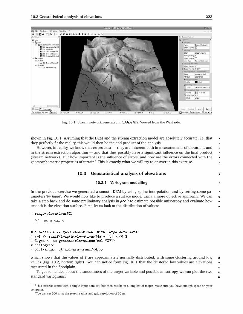
10.3 Geostatistical analysis of elevations 223
Fig. 10.1: Stream network generated in SAGA GIS. Viewed from the West side.
shown in Fig. 10.1. Assuming that the DEM and the stream extraction model are absolutely accurate, i.e. that 1
they perfectly fit the reality, this would then be the end product of the analysis. 2
However, in reality, we know that errors exist — they are inherent both in measurements of elevations and 3
in the stream extraction algorithm — and that they possibly have a significant influence on the final product 4
(stream network). But how important is the influence of errors, and how are the errors connected with the 5
geomorphometric properties of terrain? This is exactly what we will try to answer in this exercise. 6
10.3 Geostatistical analysis of elevations 7
10.3.1 Variogram modelling 8
In the previous exercise we generated a smooth DEM by using spline interpolation and by setting some pa- 9
rameters ‘by hand’. We would now like to produce a surface model using a more objective approach. We can 10
take a step back and do some preliminary analysis in geoR to estimate possible anisotropy and evaluate how 11
smooth is the elevation surface. First, let us look at the distribution of values: 12
> range(elevations$Z)
[1] 85.0 244.2
# sub-sample -- geoR cannot deal with large data sets!> sel <- runif(length(elevations@data[[1]]))<0.2> Z.geo <- as.geodata(elevations[sel,"Z"])# histogram:> plot(Z.geo, qt.col=grey(runif(4)))
which shows that the values of Z are approximately normally distributed, with some clustering around low 13
values (Fig. 10.2, bottom right). You can notice from Fig. 10.1 that the clustered low values are elevations 14
measured in the floodplain. 15
To get some idea about the smoothness of the target variable and possible anisotropy, we can plot the two 16
standard variograms: 17
3This exercise starts with a single input data set, but then results in a long list of maps! Make sure you have enough space on yourcomputer.
4You can set 500 m as the search radius and grid resolution of 30 m.
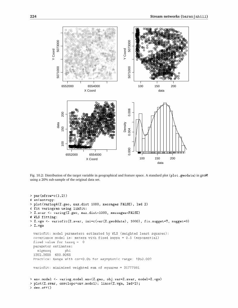
224 Stream networks (baranjahill)
6552000 6554000
5071
000
5073
000
X Coord
Y C
oord
●●●
● ●
●●●
●●●
●●●
●●
●●●
●●●●
●
● ●
●●
●
●● ●
●● ●
●●●
●
●●●● ●
●●●●
●●● ●
●●●
●
● ●●●
●
●
● ●●
●●
●●●
● ●●
●
●
●●●
● ●
●●
●
●
●●●●
●
●
●
●
●
● ●●●●
●●
●●
●●
●
●●
●
● ●●●●
●
●●●
●●●● ●
●
●
●●●
●
●
●●
● ●
●
●●
●
●●
●●●●●
●●
●●
●
●
●●
●
●●● ●●
●●
● ●
●●●
●●
●
●●
●
●●●
●
●●
●
●
●
● ●
●●
●●
●●
●
●
●
●●
●●
●
●●
●
●●
●
●●●
●
●
●
●●
● ●
●●●●
●●● ●●
●●●
●
●●● ●
● ●
●
●
● ●
●●●●
●●●
●
● ●●
●
●● ●●
●●●
●
●●●●
●●
●●
●
●●
●
●●●●●●
●
●●●●●
●●
●●
●●●
●
●
●●●
●● ●
●●
●●●
●●
●
●●●
●
●
● ●●●
●●
●●●●
●
●
●
●●
●●
●●
●●●
●
●●
●
●●
●●
●
●
●
●●
●
●
●●
●●
●
●
●
●
● ●
●●●
●●●●●●
●●
●●●
●●●●●
●●
●●
●
●●
● ●
●
●●
●●
●●
●
●
●
●●
●
●
●●●●
●
●
●●
●
●
●●
●●
●●
●
●
●●
●●
●
●
●●●
●●●
●●●
●
●●●●●
● ●●
●
●●●●
●●●●
●●●●
●
●
●●●
●●
●●●
●●●
●
●●
●●●
●●
●●
●
●
●
●●
●
●
●
● ● ●
●
●●
●
●
●
●
●●●
●●
●●●
●
●
●●
●●
●
●
●
●●●●
●
●
●
●
●●●●●
●●
●
●●
●
●
●●●●●●●
●
●●●
●●●●●
●
●
●●
●
●●
●
●
●
●●
●●
●●●●●
●
●●●●●
●
●●●
●●
●
●●●●●
●●
●
●●
●●●
●●
●●●●
●
●●●●
●●
●●
●●
●
●
●
●
●●●
●●●
●●●
●
●
●●●
●
●●
●
●●
●●
●●●
●●
●●●●●
●
●
●
●
●●●●●
●●
●●
●●
●
●●
●
●●●●●
●
●●●●●●
●●
●
●
●●●
●
●
●●●●
●
●●●
●●●●●
●●●●●●
●
●
●●
●
●●●●●
●●
●●
●●●
●●
●
●●●
●●●●
●●
●
●●●●
●
●●
●
●
●●
●● ●
●●
●
●
●
●
●
●
●●●
●
●●●
●
●●
●●
●
●●
●
●●●●
●●●
●
●●●●
●
●
●●●●
●●●
●●●
●
●●●
●●●
●●●
●
●●●●
●
●●●●●
●
●●●●
●
●●●
●●
●
●●
●
●●●
●
●
●
●●●●
●
●
●●●
●●●●●●●
●●●
●
●●
●
●●●●
●
●
●
●●●
●●●
●●●●●
●●●
●
●●●●●
●
●● ●●●
●●
●
●
●
●●
●●
●●
●●
●
●
●
●●
●●
●
●●
●●●
●
●●
●
●●
●●
●●●
●
●
●●
●●
●●●●
●
●●
●
●
●
●
●●●●●●
●
●
●
●●
●●
●
●
●
●●●●●●●
●●●
●●●●
●●●
●●●●
●●●
●
●
●
●
●
●●●●
●
●
●
●●●
●
●●
● ●●●
●●●●
●
●●●●
●●●
●
●
●●●●●●●●●
●●
●●
●●●●
●
●●●●●
●
●●●●
●●
●●●●
●●●
●
●●●
●
●●●●●
●●●
●●●●
●●
●●●●
●
●●●●
●
●
●●●●●
●●
●●●
●●●
●●●●
●●●
●
●●
●●●●●●●●
●●●
●●
●●
●●●
●
●●
●●●
●
●
●●
●●●
●
●
●●●
●
●●●
●
●●
●
●
●●●
●
●●
●
●
●●
●
●●
●●
●●●
●
●
●
●
●●●●●●●●●
●●●
●
●●●●●
●
●
●●
●
●
●●
●
●
●●
●●
●
●
●●
●●
●●●●
●●●●●
●●●●
●●●●
●●
●
●
●●
●●●●
●●●●
●●●
●
●●●●
●●●
●
●●●●
●●●●
●
●●●
●●●●●●
●
●
●●●
●●
●●
●●
●●●
●
●
●●●
●●●●●
●●●
●●
●
●
●
●●
●
●●●●●●●●●●
●●
●
●●●●
●●●●
●●●
●●●
●
●●
●●●
●●● ●
●●
●●
●●●●●
●
●
●
●
●●
●
●
● ●●●
●●●●●●
●
●●●●
●●●
●
●●●●●●
●
●●●●●
●●●●
●
●●●
●●●
●●
●●●●
●●●
●●●
●●
●●●
●●
●●
●●●●●
●●●●●
●●●
●●●
●●
●●●●
●●
●●●●
●●
●●
●●
●
●
●
●●●●
●●●●
●
●●●
●●●●●
●●●●
●
●
●●
●
●●●
●●
●
●
●●●
●
●
●●
●●
●
●●
●●
●
●
●●●
●
●●
●
●
●●●
●●●●
●●●
●
●
●
●●
●●●
●
●
●
●
●●
●●
●●
●●
●
●
●
●
●●●●
●
●
●●
●
●
●
●
●
●●
●
●●
●
●●●●
●
●●●●
●
●
●
●
●●
●●
●●
●●●
●●
●
●●
●●
●●
100 150 200
5071
000
5073
000
data
Y C
oord
●●
●
●
●
●
●
●
●
●
●
●
●
●
●●
●
●
●
●
●
●
●
●
●
●
●
●
●●
●
●●
● ●●●●●●●●
●●●●●
●
●
●●
●●
●
●
●●
●
●
●●
●
●
●●
●●
●
●
●
●
●
●●
●
●●
●●
●
●●
●●
●
●●
●
●
●
●
●
●
●
● ● ●●● ●● ●●●●●●●●●
●●●●●●●
●●● ●● ● ●●●●
● ●●●●●●●● ● ●
●
●
●
●
●●● ●●●●
●
●
●
●
●
●●
●
●●●
●
●
●
●
●
●●●
● ●●
●●●
● ●●●●●●●●●●●
●● ● ● ●●●● ●●●● ●●●●
●●●●●●●●●●●● ●●●●● ●● ● ●●●●● ● ●● ●●● ●
●●●●●
●●● ●●●● ● ●● ●● ● ●●●●●●●●●●●●●●●
●●● ● ●● ● ●●● ●● ●●●●●●●●●●●●●
●● ● ●●● ●● ●●● ●●●●●●●●●
●●●●● ● ● ●●● ●●●●●●●●●●
●
●●●● ●●●●●●●●●●
●● ● ●● ●●●●●●● ● ● ●●●●●●●●
●●● ● ● ● ●●●●●●●●● ●●●●
● ●●●●
●
●● ●●●●●●●●●●●●●
●●●●● ● ●●●
●
● ●●●●●●●●●●●●
●●●●●●●●
●●● ●●●●●●●●●
●●●●●●●●●●● ●●● ●●● ●●●
●●●●●●● ●●●● ● ●●
●●●●●●●●●●●●
●●●●●● ●●●
●● ●●● ●●●●●●
●● ● ●● ●●●●●●●●●●●●●●
● ●●●●
●●●●
●●●●●●●●●●●
●●●
●
●●
●●
●●● ●●● ● ●●●●●●● ●●●●● ●●● ●●
●●●
●●●●
●●● ●●●
●
●●
●●●●●●
●●●
●●
●● ●●●●●●●●●● ●●●●● ● ●●●
●●●●●
●●●●
●● ●●●●●●●●
●●●●
●
●●●●●●●●● ● ●●●● ●●●
●
●●
●
●●● ●●●●●●● ●●● ● ●●●●●● ●●●● ●
●● ●●●●●●●●●●●●●●●● ● ●
●●● ●●●●● ● ●
● ●●●●● ●●●● ●●●●●●●● ● ●●
●●●●●● ● ●●●● ●●●●●●● ●
●●●●●● ●●●●●●● ●
●●●
●●● ●●●●● ●●
●●●●●●●●● ●●●●●●●● ● ●● ●
●●●●●●● ●●
●●●●●●●●●● ●●●● ● ●
●●●●● ● ● ●
●●●●●●●●●●●●●●
●
●●●●●●● ●●
●●●
●●●●● ●●●●●●●● ●● ●●●●●●● ●● ●●●● ● ●●●●●●●●● ●●●●● ● ●● ●●●●●●●●●●●●●
● ●
●●●●●●●●●●●●● ●●● ●
●●●●●●●●
●● ●●●●●●●
● ●●
●●●● ● ●●●● ●● ●●●●●●
● ●●●● ●●●●●
●●● ●●●●
● ●●●●●
●
●●●●
●●●●●
●
●
●
●
●● ●
●●
●●●●● ●●●
●●
●●●
●●●●● ●●●●●● ●
●● ●●●●●●●● ●●
●●●● ●●●●●●
●●● ●● ●●●●●●●●
●●●●● ● ●●●●●●●
●●●● ●●●●●●●●●●●●●●● ●●
●● ●●●●●●●●●●●
● ●●●●●●●●●●
●●●
●●●
●●●●
●●
●●
●●●●●●●●●
●●●
●●●●●●●
●●●●●●●●●●
●●●●● ●●●●●●●●●●
●●●● ●
●
●●●●● ●● ● ●●●●●●●●●●
●●● ●● ●●●●●●●
●● ●●●● ●●●●
●●
● ●
●●●●●
●●
●●
●
●●●●
6552000 6554000
100
150
200
X Coord
data
data
Den
sity
100 150 200
0.00
00.
004
0.00
8
Fig. 10.2: Distribution of the target variable in geographical and feature space. A standard plot (plot.geodata) in geoR
using a 20% sub-sample of the original data set.
> par(mfrow=c(1,2))# anisotropy:> plot(variog4(Z.geo, max.dist=1000, messages=FALSE), lwd=2)# fit variogram using likfit:> Z.svar <- variog(Z.geo, max.dist=1000, messages=FALSE)# WLS fitting:> Z.vgm <- variofit(Z.svar, ini=c(var(Z.geo$data), 1000), fix.nugget=T, nugget=0)> Z.vgm
variofit: model parameters estimated by WLS (weighted least squares):covariance model is: matern with fixed kappa = 0.5 (exponential)fixed value for tausq = 0parameter estimates:
sigmasq phi1352.3685 650.9268Practical Range with cor=0.05 for asymptotic range: 1950.002
variofit: minimised weighted sum of squares = 31777661
> env.model <- variog.model.env(Z.geo, obj.var=Z.svar, model=Z.vgm)> plot(Z.svar, envelope=env.model); lines(Z.vgm, lwd=2);> dev.off()
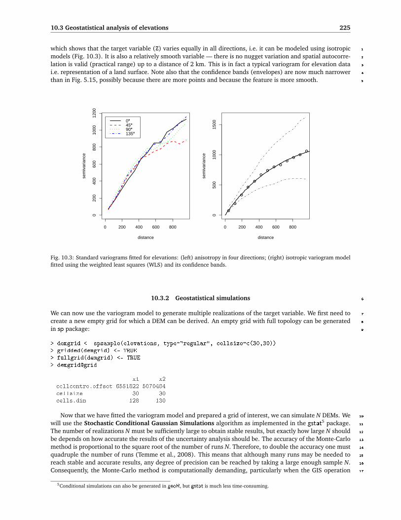
10.3 Geostatistical analysis of elevations 225
which shows that the target variable (Z) varies equally in all directions, i.e. it can be modeled using isotropic 1
models (Fig. 10.3). It is also a relatively smooth variable — there is no nugget variation and spatial autocorre- 2
lation is valid (practical range) up to a distance of 2 km. This is in fact a typical variogram for elevation data 3
i.e. representation of a land surface. Note also that the confidence bands (envelopes) are now much narrower 4
than in Fig. 5.15, possibly because there are more points and because the feature is more smooth. 5
0 200 400 600 800
020
040
060
080
010
0012
00
distance
sem
ivar
ianc
e
0°°45°°90°°135°°
●
●
●
●
●
●
●
●●
●
●●
●
0 200 400 600 800
050
010
0015
00
distance
sem
ivar
ianc
e
Fig. 10.3: Standard variograms fitted for elevations: (left) anisotropy in four directions; (right) isotropic variogram modelfitted using the weighted least squares (WLS) and its confidence bands.
10.3.2 Geostatistical simulations 6
We can now use the variogram model to generate multiple realizations of the target variable. We first need to 7
create a new empty grid for which a DEM can be derived. An empty grid with full topology can be generated 8
in sp package: 9
> demgrid <- spsample(elevations, type="regular", cellsize=c(30,30))> gridded(demgrid) <- TRUE> fullgrid(demgrid) <- TRUE> demgrid@grid
x1 x2cellcentre.offset 6551822 5070484cellsize 30 30cells.dim 128 130
Now that we have fitted the variogram model and prepared a grid of interest, we can simulate N DEMs. We 10
will use the Stochastic Conditional Gaussian Simulations algorithm as implemented in the gstat5 package. 11
The number of realizations N must be sufficiently large to obtain stable results, but exactly how large N should 12
be depends on how accurate the results of the uncertainty analysis should be. The accuracy of the Monte-Carlo 13
method is proportional to the square root of the number of runs N. Therefore, to double the accuracy one must 14
quadruple the number of runs (Temme et al., 2008). This means that although many runs may be needed to 15
reach stable and accurate results, any degree of precision can be reached by taking a large enough sample N. 16
Consequently, the Monte-Carlo method is computationally demanding, particularly when the GIS operation 17
5Conditional simulations can also be generated in geoR, but gstat is much less time-consuming.

226 Stream networks (baranjahill)
takes significant computing time (Heuvelink, 2002). As a rule of thumb, we will take 100 simulations as large1
enough.2
Because we further use gstat, we need to copy the fitted variogram values to a vgm object:3
# copy the values fitted in geoR:> Z.ovgm <- vgm(psill=Z.vgm$cov.pars[1], model="Mat",+ range=Z.vgm$cov.pars[2], nugget=Z.vgm$nugget, kappa=1.2)> Z.ovgm
model psill range kappa1 Nug 0.000 0.0000 02 Mat 1352.368 650.9268 1.2
Fig. 10.4: Four realizations of the DEM following conditional geostatistical simulations.
Note that we have purposively set the kappa6 parameter at 1.2 (it was originally 0.5). Following our4
knowledge about the feature of interest, we know that a land surface is inherently smooth — due to the5
erosional processes and permanent leveling of topography — so we wish to generate realizations of DEMs that6
fit our knowledge of the area.7
The conditional simulations in gstat can be run by simply adding the nsim argument to the generic krige8
method:9
> N.sim <- 100> DEM.sim <- krige(Z ∼ 1, elevations, demgrid, Z.ovgm, nmax=30, nsim=N.sim)
drawing 100 GLS realisations of beta...
# this can take few minutes!!> fullgrid(DEM.sim) <- TRUE> spplot(DEM.sim[1:4], col.regions=grey(seq(0,1,0.025)))
which shows that we have accomplished our objective: we have managed to simulate 100 equiprobable DEMs10
that are equally smooth as the DEM shown in Fig. 10.1. To visualize the differences between realizations, we11
can make a cross section and plot all simulated surfaces on top of each other (Fig. 10.5):12
# Cross-section at y=5,073,012:> cross.s <- data.frame(X=seq(demgrid@bbox[1,1]+gridcell/2,+ demgrid@bbox[1,2]-gridcell/2, gridcell), Y=rep(5073012, demgrid@[email protected][1]))> coordinates(cross.s) <- ∼ X+Y# proj4string(cross.s) <- elevations@proj4string> cross.ov <- overlay(DEM.sim, cross.s)> plot(cross.ov@coords[,1], cross.ov@data[[1]], type="l", xlab="X",+ ylab="Z", col="grey")> for(i in 2:N.sim-1){> lines(cross.ov@coords[,1], cross.ov@data[[i]], col="grey")> }> lines(cross.ov@coords[,1], cross.ov@data[[N.sim]], lwd=2)

10.4 Generation of stream networks 227
6552000 6553000 6554000 6555000
100
150
200
X
Z
Fig. 10.5: 100 simulations of DEM showing using a cross-section from West to East (cross-section at X=5,073,012).Compare with Temme et al. (2008, p.130).
You will notice that the confidence band is relatively wide (few meters). The confidence band is controlled 1
with the density of sampling locations — the further you get from sampling locations, the higher will be the 2
error. This property we will further explore in §10.5. 3
Why is a high kappa parameter necessary? If you run DEM simulations with e.g. an exponential model, 4
you will see that the realizations will be much noisier than what we would expect (Hengl et al., 2008). This 5
will happen even if you set the nugget parameters at zero (smooth feature). There are several explanations for 6
this. Having a non-zero grid resolution implies that the correlation between adjacent grid cells is not equal to 7
1, so that grids may still appear to have noise (Temme et al., 2008). A noisy DEM leads to completely different 8
drainage networks — the streams will be shorter and more random — which we know does not fit knowledge 9
about the area. The Matérn variogram model (Eq.1.3.10), on the other hand, allow us to produce smoother 10
DEMs, while still using objectively estimated nugget, sill and range parameters. This makes it especially 11
suitable for modeling of land surface. 12
10.4 Generation of stream networks 13
Now that we have simulated N DEMs, we can derive stream networks using the “Channel Network” function, 14
which is available also via the command line i.e. via the ta_channels SAGA library. To get complete info 15
about this module you can use: 16
> rsaga.get.usage("ta_channels", 0)
First, convert the maps to SAGA format: 17
# write simulated DEMs to SAGA format:> for(i in 1:N.sim){> write.asciigrid(DEM.sim[i], paste("DEM", i, ".asc", sep=""), na.value=-1)> }# get a list of files:> dem.list <- list.files(getwd(), pattern="DEM[[:digit:]]*.asc")> rsaga.esri.to.sgrd(in.grids=dem.list, out.sgrd=set.file.extension(dem.list,+ ".sgrd"), in.path=getwd(), show.output.on.console=FALSE)> unlink(dem.list)
Recall that, before we derive a stream network, we also want to remove7 spurious sinks. For this we can 18
use e.g. the method of Planchon and Darboux (2001): 19
6See Diggle and Ribeiro Jr (2007, p.51–53).7This is also based on the empirical knowledge: water typically erodes small obstacles and creates continuous paths.

228 Stream networks (baranjahill)
> stream.list <- list(rep(NA, N.sim))> for (i in 1:N.sim) {# First, filter the spurious sinks:> rsaga.geoprocessor(lib="ta_preprocessor", module=2,+ param=list(DEM=paste("DEM", i, ".sgrd", sep=""),+ RESULT="DEMflt.sgrd", MINSLOPE=0.05), show.output.on.console=FALSE)# Second, extract the channel network:> rsaga.geoprocessor(lib="ta_channels", module=0, param=list(ELEVATION="DEMflt.sgrd",+ CHNLNTWRK=paste("channels", i, ".sgrd", sep=""), CHNLROUTE="channel_route.sgrd",+ SHAPES="channels.shp", INIT_GRID="DEMflt.sgrd", DIV_CELLS=3, MINLEN=40),+ show.output.on.console=FALSE)# read vector maps into R:> stream.list[[i]] <- readOGR("channels.shp", "channels")> proj4string(stream.list[[i]]) <- elevations@proj4string> }
Here we use arbitrary input parameters for the minimum length of streams (40) and initial grid, but this is1
not relevant for this exercise. Note that we do not really need all maps, but only the vector map showing the2
position of streams. Therefore, we can recycle temporary maps in each loop.3
Once the processing is finished, we can visualize all derived streams on top of each other:4
# plot all derived streams on top of each other:> stream.plot <- as.list(rep(NA, N.sim))> for(i in 1:N.sim){> stream.plot[[i]] <- list("sp.lines", stream.list[[i]])> }> lines.plt <- spplot(DEM.sim[1], col.regions=grey(seq(0.5,1,0.025)),+ scales=list(draw=T), sp.layout=stream.plot, main="100 streams")
Fig. 10.6: 100 realizations of stream network overlaid on top of each other (left); probability of stream network, overlaidwith one realization (right).
which is shown in Fig. 10.6 (left). This visualization of density of streams illustrates the concept of propagated5
uncertainty. If you zoom in into this map, you will notice that the streams follow the gridded-structure of the6
DEMs, which explains some artificial breaks in the lines.7
To actually derive a probability of mapping a stream, we need to import all gridded maps of streams, then8
count how many times the model estimated a stream over a certain grid node:9
# get the list of maps:> streamgrid.list <- list.files(getwd(), pattern="channels[[:digit:]]*.sgrd")

10.5 Evaluation of the propagated uncertainty 229
> rsaga.sgrd.to.esri(in.sgrds=streamgrid.list,+ out.grids=set.file.extension(streamgrid.list, ".asc"),+ out.path=getwd(), prec=0, show.output.on.console=FALSE)# read all grids into R:> streamgrid <- readGDAL(set.file.extension(streamgrid.list[[1]], ".asc"))> streamgrid@data[[1]] <- ifelse(streamgrid$band1<0, 0, 1)> for(i in 2:length(streamgrid.list)){> tmp <- readGDAL(set.file.extension(streamgrid.list[[i]], ".asc"))# convert to a binary map:> streamgrid@data[[i]] <- ifelse(tmp$band1<0, 0, 1)> }> names(streamgrid) <- set.file.extension(streamgrid.list, ".asc")> proj4string(streamgrid) <- elevations@proj4string
Now we have a pack of grids (streamgrid), with 0/1 values depending on the stream occurrence (yes/no). 1
These can be summed using the rowSums method: 2
> streamgrid$pr <- rowSums(streamgrid@data, na.rm=TRUE, dims=1)/length(streamgrid@data)
and the probability of detecting a stream is simply the average value of stream from multiple simulations. This 3
map is shown in Fig. 10.6 (right): 4
> stream.plt <- spplot(streamgrid["pr"], col.regions=grey(rev((1:59)/60)),+ scales=list(draw=T), sp.layout=list("sp.lines", stream.list[[1]]),+ main="Stream (probability)")> print(lines.plt, split=c(1,1,2,1), more=TRUE)> print(stream.plt, split=c(2,1,2,1), more=FALSE)
Next, we would like to derive the propagated uncertainty of mapping a stream. Theoretically speaking, 5
stream is a discrete feature that follows a Bernoulli distribution which takes value 1 with success probability 6
p and value 0 with failure probability q=1 − p. Thus the error of mapping a stream can be derived as: 7
−q ln(q)− p ln(p), or in R syntax: 8
> streamgrid$pr.var <- -streamgrid$pr*log2(streamgrid$pr)+ -(1-streamgrid$pr)*log2(1-streamgrid$pr)
which means that the highest uncertainty of mapping a stream is when p approaches 0.5 (equal probability 9
of stream and not-stream). As anticipated, the propagated variability of detecting a stream is much higher (in 10
cumulative terms) in the terrace region of the study area (Fig. 10.5). The remaining issue is whether we could 11
explain this variability using some topographic, land surface parameters. 12
10.5 Evaluation of the propagated uncertainty 13
Now that we have estimated the propagated uncertainty of extracting channel networks (streams) from DEMs, 14
we can try to understand how this uncertainty relates to the geomorphology of terrain. We will derive and 15
run a comparison by using only a few land surface parameters; you might consider extending the list. First, 16
we can derive mean value (the ‘most probable’ DEM) and standard deviation i.e. the propagated uncertainty 17
of mapping elevation: 18
> rsaga.geoprocessor(lib="geostatistics_grid", module=5,+ param=list(GRIDS=paste(set.file.extension(dem.list,".sgrd"), collapse=";"),+ MEAN="DEM_avg.sgrd", STDDEV="DEM_std.sgrd"), show.output.on.console=FALSE)> rsaga.sgrd.to.esri(in.sgrds=c("DEM_avg.sgrd","DEM_std.sgrd"),+ out.grids=c("DEM_avg.asc","DEM_std.asc"), out.path=getwd(), prec=2)
Next, it is interesting to derive a map of slope, as it largely controls the hydrological properties, and the 19
difference from the mean value in 5×5 search radius 8: 20
8Note that these are wrapper function, which means that they combine several operations together — in this case derivation of slopeand conversion of maps to ArcInfo ASCII format.

230 Stream networks (baranjahill)
Fig. 10.7: Relationship between the standard error of interpolating elevation and local slope; and probability of derivingstreams and difference from the mean elevation.
# slope:> rsaga.esri.wrapper(rsaga.slope, method="poly2zevenbergen", in.dem="DEM_avg.sgrd",+ out.slope="SLOPE.sgrd", prec=3, clean.up=F)# residual analysis:> rsaga.geoprocessor(lib="geostatistics_grid", 0, param=list(INPUT="DEM_avg.sgrd",+ MEAN="tmp.sgrd", STDDEV="tmp.sgrd", RANGE="tmp.sgrd", DEVMEAN="tmp.sgrd",+ PERCENTILE="tmp.sgrd", RADIUS=5, DIFF="DIFMEAN.sgrd"))
and then read back the results to R:1
> rsaga.sgrd.to.esri(in.sgrds=c("DEM_avg.sgrd","DEM_std.sgrd", "DIFMEAN.sgrd"),+ out.grids=c("DEM_avg.asc","DEM_std.asc", "DIFMEAN.asc"), out.path=getwd(), prec=2)# read back into R:> gridmaps <- readGDAL("DEM_avg.asc")> names(gridmaps) <- "DEM"> gridmaps$std <- readGDAL("DEM_std.asc")$band1> gridmaps$SLOPE <- readGDAL("SLOPE.asc")$band1> gridmaps$DIFMEAN <- readGDAL("DIFMEAN.asc")$band1
Which allows us to plot the two DEM parameters versus the probability of finding stream and propagated2
DEM error:3
> par(mfrow=c(1,2))> scatter.smooth(gridmaps$SLOPE, gridmaps$std, span=18/19, col="grey",+ xlab="Slope", ylab="DEM error", pch=19)> scatter.smooth(streamgrid$pr[streamgrid$pr>0], gridmaps$DIFMEAN[streamgrid$pr>0],+ span=18/19, col="grey", xlab="Stream probability", ylab="Dif. from mean", pch=19)> dev.off()
Fig. 10.7 shows two interesting things: (1) the errors in elevations are largely controlled by the slope; (2)4
streams are especially difficult to map in areas where the difference from the mean value is high, i.e. close5
to zero or positive (meaning areas with low local relief or close to concave shapes). This largely reflects our6
expectation, but it is rewarding to be able to prove these assumptions using hard data.7

10.6 Advanced exercises 231
Fig. 10.8: Scatter plot in SAGA GIS. This is the same plot asshown in Fig. 10.7.
Optional: open all derived maps in SAGA and 1
visualize correlations between the probability of 2
streams and DEM error versus various DEM param- 3
eters using the scatter plot option. To produce a 4
plot shown in Fig. 10.8 right click on the raster map 5
of interest (DEM_std) and then select “Show scatter- 6
plot” 7→ select grid. You can adjust the size of grid 7
cells and default representation in this plot by edit- 8
ing properties (from the main menu). 9
10.6 Advanced exercises 10
10.6.1 Objective selection of the grid cell size 11
In the previous exercise we set the grid cell size 12
at 30 m, without any real justification. Now we 13
can consider statistically sound approach to select a 14
grid cell size based on the accuracy of the derived 15
stream network. This follows the idea of Hutchin- 16
son (1996), who use an iterative DEM cell-size opti- 17
mization algorithm as implemented in theANUDEM 18
package. By plotting the error of mapping streams 19
versus the grid spacing index, one can select the grid 20
cell size that shows the maximum information content in the final map. The optimal grid cell size is the one 21
where further refinement does not change the accuracy of derived streams. 22
We can implement this principle using our case study, i.e. we can derive drainage networks using several 23
grid cell sizes and then see if the spatial location of streams differs significantly from the one derived using the 24
finest resolution (see Fig. 10.9). We can start with generating DEMs from point data (e.g. using splines) using 25
a range of grid cell sizes: 26
> pixel.range <- c(20, 30, 40, 50, 60, 80, 100)# generate DEMs using splines:> for(i in 1:length(pixel.range)){> rsaga.geoprocessor(lib="grid_spline", module=1,+ param=list(GRID=paste("DEMpix", pixel.range[i], ".sgrd", sep=""),+ SHAPES="elevations.shp", FIELD=1, RADIUS=sqrt(areaSpatialGrid(demgrid))/3,+ SELECT=1, MAXPOINTS=10, TARGET=0, USER_CELL_SIZE=pixel.range[i],+ USER_X_EXTENT_MIN=demgrid@bbox[1,1]+pixel.range[i]/2,+ USER_X_EXTENT_MAX=demgrid@bbox[1,2]-pixel.range[i]/2,+ USER_Y_EXTENT_MIN=demgrid@bbox[2,1]+pixel.range[i]/2,+ USER_Y_EXTENT_MAX=demgrid@bbox[2,2]-pixel.range[i]/2))> }
Next, we can derive stream networks for each DEM, and then buffer distance to the stream network using 27
a loop. We set the minimum length of stream (min.len) based on the cell size of DEM: 28
# estimate drainage map for each DEM:> for(i in 1:length(pixel.range)){# filter the spurious sinks:> rsaga.geoprocessor(lib="ta_preprocessor", module=2,+ param=list(DEM=paste("DEMpix", pixel.range[i], ".sgrd", sep=""),+ RESULT="DEMflt.sgrd", MINSLOPE=0.05), show.output.on.console=FALSE)# minimum length:> min.len <- round(sqrt(areaSpatialGrid(demgrid))/(pixel.range[i]*3.5), 0)# extract the channel network:> rsaga.geoprocessor(lib="ta_channels", module=0,+ param=list(ELEVATION="DEMflt.sgrd", CHNLNTWRK=paste("chnlntwrk_pix",+ pixel.range[i], ".sgrd", sep=""), CHNLROUTE="tmp.sgrd",+ SHAPES=paste("channels_pix", i, ".shp", sep=""), INIT_GRID="DEMflt.sgrd",

232 Stream networks (baranjahill)
Fig. 10.9: Drainage network derived using different grid cell sizes.
+ DIV_CELLS=3, MINLEN=min.len), show.output.on.console=FALSE)# buffer distance to actual streams (use the finest grid cell size):> rsaga.geoprocessor(lib="grid_gridding", module=0,+ param=list(GRID="stream_pix.sgrd",+ INPUT=paste("channels_pix", i, ".shp", sep=""), FIELD=1, LINE_TYPE=0,+ USER_CELL_SIZE=pixel.range[1],+ USER_X_EXTENT_MIN=demgrid@bbox[1,1]+pixel.range[1]/2,+ USER_X_EXTENT_MAX=demgrid@bbox[1,2]-pixel.range[1]/2,+ USER_Y_EXTENT_MIN=demgrid@bbox[2,1]+pixel.range[1]/2,+ USER_Y_EXTENT_MAX=demgrid@bbox[2,2]-pixel.range[1]/2),+ show.output.on.console=FALSE)# extract a buffer distance map:> rsaga.geoprocessor(lib="grid_tools", module=10,+ param=list(SOURCE="stream_pix.sgrd", DISTANCE="tmp.sgrd",+ ALLOC="tmp.sgrd", BUFFER=paste("buffer_pix", pixel.range[i], ".sgrd", sep=""),+ DIST=2000, IVAL=pixel.range[1]), show.output.on.console=FALSE)> }
and then read maps into R:1
> rsaga.sgrd.to.esri(in.sgrds="chnlntwrk_pix20.sgrd",+ out.grids="chnlntwrk_pix20.asc", out.path=getwd(), prec=1)> griddrain <- readGDAL("chnlntwrk_pix20.asc")> names(griddrain) <- "chnlntwrk"> for(i in 2:length(pixel.range)){> rsaga.sgrd.to.esri(in.sgrds=paste("buffer_pix", pixel.range[i], ".sgrd", sep=""),+ out.grids=paste("buffer_pix", pixel.range[i], ".asc", sep=""),+ out.path=getwd(), prec=1)> griddrain@data[paste("buffer_pix", pixel.range[i], sep="")] <-+ readGDAL(paste("buffer_pix", pixel.range[i], ".asc", sep=""))$band1> }> str(griddrain@data)
'data.frame': 37440 obs. of 7 variables:$ chnlntwrk : num NA NA NA NA NA NA NA NA NA NA ...$ buffer_pix30 : num 500 500 480 460 460 440 420 420 400 400 ...$ buffer_pix40 : num 500 480 460 460 440 420 420 400 400 380 ...$ buffer_pix50 : num 520 500 500 480 460 460 440 440 420 420 ...
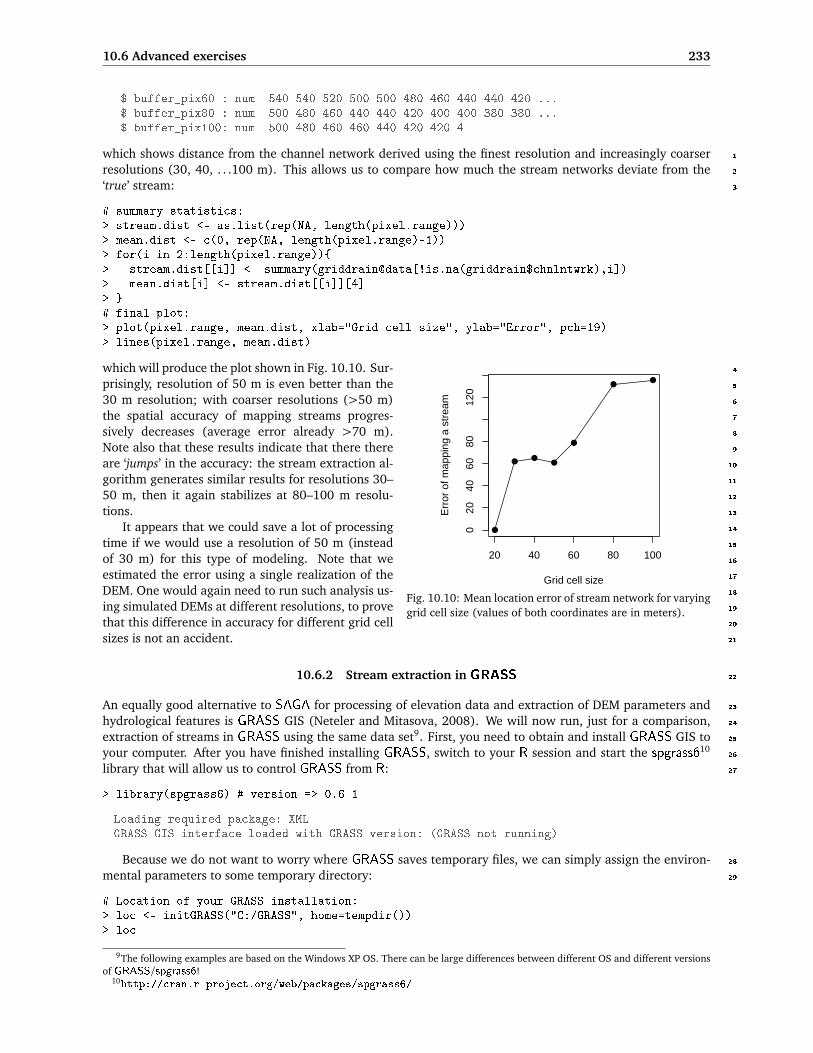
10.6 Advanced exercises 233
$ buffer_pix60 : num 540 540 520 500 500 480 460 440 440 420 ...$ buffer_pix80 : num 500 480 460 440 440 420 400 400 380 380 ...$ buffer_pix100: num 500 480 460 460 440 420 420 4
which shows distance from the channel network derived using the finest resolution and increasingly coarser 1
resolutions (30, 40, . . .100 m). This allows us to compare how much the stream networks deviate from the 2
‘true’ stream: 3
# summary statistics:> stream.dist <- as.list(rep(NA, length(pixel.range)))> mean.dist <- c(0, rep(NA, length(pixel.range)-1))> for(i in 2:length(pixel.range)){> stream.dist[[i]] <- summary(griddrain@data[!is.na(griddrain$chnlntwrk),i])> mean.dist[i] <- stream.dist[[i]][4]> }# final plot:> plot(pixel.range, mean.dist, xlab="Grid cell size", ylab="Error", pch=19)> lines(pixel.range, mean.dist)
●
●●
●
●
●●
20 40 60 80 100
020
4060
8012
0
Grid cell size
Err
or o
f map
ping
a s
trea
m
Fig. 10.10: Mean location error of stream network for varyinggrid cell size (values of both coordinates are in meters).
which will produce the plot shown in Fig. 10.10. Sur- 4
prisingly, resolution of 50 m is even better than the 5
30 m resolution; with coarser resolutions (>50 m) 6
the spatial accuracy of mapping streams progres- 7
sively decreases (average error already >70 m). 8
Note also that these results indicate that there there 9
are ‘jumps’ in the accuracy: the stream extraction al- 10
gorithm generates similar results for resolutions 30– 11
50 m, then it again stabilizes at 80–100 m resolu- 12
tions. 13
It appears that we could save a lot of processing 14
time if we would use a resolution of 50 m (instead 15
of 30 m) for this type of modeling. Note that we 16
estimated the error using a single realization of the 17
DEM. One would again need to run such analysis us- 18
ing simulated DEMs at different resolutions, to prove 19
that this difference in accuracy for different grid cell 20
sizes is not an accident. 21
10.6.2 Stream extraction in GRASS 22
An equally good alternative to SAGA for processing of elevation data and extraction of DEM parameters and 23
hydrological features is GRASS GIS (Neteler and Mitasova, 2008). We will now run, just for a comparison, 24
extraction of streams in GRASS using the same data set9. First, you need to obtain and install GRASS GIS to 25
your computer. After you have finished installing GRASS, switch to your R session and start the spgrass61026
library that will allow us to control GRASS from R: 27
> library(spgrass6) # version => 0.6-1
Loading required package: XMLGRASS GIS interface loaded with GRASS version: (GRASS not running)
Because we do not want to worry where GRASS saves temporary files, we can simply assign the environ- 28
mental parameters to some temporary directory: 29
# Location of your GRASS installation:> loc <- initGRASS("C:/GRASS", home=tempdir())> loc
9The following examples are based on the Windows XP OS. There can be large differences between different OS and different versionsof GRASS/spgrass6!
10http://cran.r-project.org/web/packages/spgrass6/

234 Stream networks (baranjahill)
gisdbase c:/WINNT/profiles/software/LOCALS∼1/Temp/RtmpdeK5s9location file678418bemapset file3d6c4ae1rows 1columns 1north 1south 0west 0east 1nsres 1ewres 1projection NA
Note that these settings are in fact nonsense. We will soon replace these with the actual parameters once1
we import an actual raster map. What is important is that we have established a link with GRASS and set the2
working directory. We can proceed with importing the previously derived DEM into GRASS:3
> parseGRASS("r.in.gdal") # commmand description
Command: r.in.gdalDescription: Import GDAL supported raster file into a binary raster map layer.Keywords: raster, importParameters:name: input, type: string, required: no, multiple: no[Raster file to be imported]...
# Import the ArcInfo ASCII file to GRASS:> execGRASS("r.in.gdal", flags="o", parameters=list(input="DEM_avg.asc", output="DEM"))
WARNING: Over-riding projection check
RINGDA∼1 complete. Raster map <DEM> created.
We can use the parameters of the imported map to set up the geographic region:4
> execGRASS("g.region", parameters=list(rast="DEM"))> gmeta6()
gisdbase c:/WINNT/profiles/software/LOCALS∼1/Temp/RtmpdeK5s9location file678418bemapset file3d6c4ae1rows 130columns 128north 5074369south 5070469west 6551807east 6555647nsres 30ewres 30projection NA
which is the averaged DEM from multiple realizations derived in §10.5. Note that Windows system generates5
the temporary name of the mapset and location. Again, we do not worry too much about this because we use6
GRASS as an external application to run geographical analysis; temporary files will be recycled, at the end we7
will read only the final results back into R.8
We proceed with the extraction of the drainage network:9
# extract the drainage network:> execGRASS("r.watershed", flags=c("m", "overwrite"),+ parameters=list(elevation="DEM", stream="stream", threshold=as.integer(50)))

10.6 Advanced exercises 235
SECTION 1 beginning: Initiating Variables. 5 sections total.SECTION 1b (of 5): Determining Offmap Flow.
SECTION 2: A * Search.
SECTION 3: Accumulating Surface Flow.
SECTION 4: Watershed determination.
SECTION 5: Closing Maps.
Fig. 10.11: Example of a screen shot — drainage extraction steps using the Baranja hill data set in GRASS GIS.
which will generate a raster map showing the position of streams (Fig. 10.11). Note that GRASS typically 1
generates a rich output with many technical details of interest to a specialist. Before we can convert the 2
derived map to a vector layer, we need to thin it: 3
> execGRASS("r.thin", parameters=list(input="stream", output="streamt"))
File stream -- 130 rows X 128 columnsBounding box: l = 2, r = 129, t = 2, b = 131Pass number 1Deleted 55 pixelsPass number 2Deleted 0 pixelsThinning completed successfully.Output file 130 rows X 128 columnsWindow 130 rows X 128 columns
# convert to vectors:> execGRASS("r.to.vect", parameters=list(input="streamt",+ output="streamt", feature="line"))

236 Stream networks (baranjahill)
WARNING: Default driver / database set to:driver: dbfdatabase: $GISDBASE/$LOCATION_NAME/$MAPSET/dbf/
Extracting lines...
Building topology for vector map <streamt>...Registering primitives...
165 primitives registered652 vertices registeredBuilding areas...
0 areas built0 isles builtAttaching islands...Attaching centroids...
Number of nodes: 176Number of primitives: 165Number of points: 0Number of lines: 165Number of boundaries: 0Number of centroids: 0Number of areas: 0Number of isles: 0RTOVEC ∼1 complete.
Processing is now complete, so we can read the produced map from R. For this, we use the generic spgrass61
command that reads any type of GRASS vector:2
# read the generated stream network map into R:> streamt <- readVECT6("streamt")
Exporting 165 points/lines...
165 features writtenOGR data source with driver: ESRI ShapefileSource: "c:/WINNT/profiles/software/LOCALS∼1/Temp/RtmpdeK5s9/file3d6c4ae1/.tmp",layer: "streamt"with 165 rows and 3 columnsFeature type: wkbLineString with 2 dimensions
> plot(streamt)
which shows a similar result as shown in Fig. 10.1. You can now open all maps you have generated and3
visualize them in GRASS. Fig. 10.11 will give you some idea about the GRASS interface. In summary, there4
are noticable differences in the ways the things are run with SAGA and GRASS. GRASS seem to be more de-5
manding considering the control of the package. On the other hand, it is a much larger and more international6
project than SAGA. It is really a question of taste if one prefers to use one or the other, but there are also no7
obstacles to combine them.8
10.6.3 Export of maps to GE9
In the final step we will export the stream probability map from R to Google Earth, this time without using10
SAGA GIS11. We can start by re-projecting the derived grid to the latitude longitude system:11
> streamgrid.ll <- spTransform(streamgrid["pr"], CRS("+proj=longlat +datum=WGS84"))> streamgrid.ll@bbox
11This is somewhat more complicated. Compare with §5.6.2.

10.6 Advanced exercises 237
min maxx 18.66122 18.71065y 45.77646 45.81158
which will create a point map (not a grid!), which means that we need to create the grid topology in the 1
longlat coordinate system ourselves. To do this, we first need to estimate the grid cell size in arcdegrees, e.g. 2
by using the Eq.(3.3.1) explained in §3.3.1. The width correction factor12 based on the latitude of the center 3
of the study area, can be estimated as: 4
> corrf <- (1 + cos((streamgrid.ll@bbox[1, "max"] ++ streamgrid.ll@bbox[2, "min"])/2 * pi/180))/2
and then the grid cell size in arcdegrees is approximately: 5
> geogrd.cell <- corrf*(streamgrid.ll@bbox[1,"max"] -+ streamgrid.ll@bbox[1, "min"]) / streamgrid@[email protected][1]> geogrd.cell
[1] 0.0003564123
which means that a width of a 30 m pixel at this latitude corresponds to about 1.3 arcseconds. 6
Fig. 10.12: Baranja hill and derived stream probability, visualized in Google Earth.
Once we have estimated the grid cell size in geographical coordinates, we can also generate the new grid 7
system: 8
> geoarc <- spsample(streamgrid.ll, type ="regular", cellsize=c(geogrd.cell, geogrd.cell))> gridded(geoarc) <- TRUE> gridparameters(geoarc)
cellcentre.offset cellsizex1 18.66127 0.0003564123x2 45.77662 0.0003564123
cells.dimx1 139x2 99
12For data sets in geographical coordinates, a cell size correction factor can be estimated as a function of the latitude and spacing at theequator.

238 Stream networks (baranjahill)
> geoarc.grid <- SpatialGridDataFrame(geoarc@grid,+ data=data.frame(rep(1, length([email protected]))),+ proj4string=streamgrid.ll@proj4string)
Now we need to estimate values of our target variable at the new grid nodes. We use the interp method1
as implemented in the akima package, which leads to a simple bilinear resampling:2
> library(akima)> streamgrid.llgrd <- interp(x=streamgrid.ll@coords[,1], y=streamgrid.ll@coords[, 2],+ z=streamgrid.ll$pr, xo=seq(geoarc.grid@bbox[1, "min"], geoarc.grid@bbox[1, "max"],+ length=geoarc.grid@[email protected][[1]]), yo=seq(geoarc.grid@bbox[2, "min"],+ geoarc.grid@bbox[2, "max"], length=geoarc.grid@[email protected][[2]]),+ linear=TRUE, extrap=FALSE)# convert to sp class:> streamgrid.llgrd <- as(as.im(streamgrid.llgrd), "SpatialGridDataFrame")> proj4string(streamgrid.llgrd) <- CRS("+proj=longlat +datum=WGS84")# mask the "0" values:> streamgrid.llgrd$pr <- ifelse(streamgrid.llgrd$v < 0.05, NA, streamgrid.llgrd$v)
which allows us to finally generate a KML ground overlay for Google Earth (Fig. 10.12):3
> streamgrid.kml <- GE_SpatialGrid(streamgrid.llgrd)> png(file="stream.png", width=streamgrid.kml$width,+ height=streamgrid.kml$height, bg="transparent")> par(mar=c(0, 0, 0, 0), xaxs="i", yaxs="i")> image(as.image.SpatialGridDataFrame(streamgrid.llgrd["pr"]),+ col=rev(), xlim=streamgrid.kml$xlim,+ ylim=streamgrid.kml$ylim)> kmlOverlay(streamgrid.kml, "stream.kml", "stream.png",+ name="Stream probability")
[1] "<?xml version='1.0' encoding='UTF-8'?>"[2] "<kml xmlns='http://earth.google.com/kml/2.0'>"[3] "<GroundOverlay>"[4] "<name>Stream probability</name>"[5] "<Icon><href>stream.png</href><viewBoundScale>0.75</viewBoundScale></Icon>"[6] "<LatLonBox><north>45.8119041798664</north><south>45.7762593102449</south>
<east>18.7108375328584</east><west>18.6609075254189</west></LatLonBox>"[7] "</GroundOverlay></kml>"
> dev.off()
windows2
Visualization of generated maps in Google Earth is important for several reasons: (1) we can check if the4
coordinate system definition is correct; (2) we can evaluate and interpret the results of mapping using high5
resolution satellite imagery; (3) Google Earth allows 3D exploration of data, which is ideal for this type of6
exercise (read more in §3.3.1).7
Before closing the R session, it is also advisable to clean up all the temporary files:8
> save.image(".RData")> unlink("*.hgrd")> unlink("*.sgrd")> unlink("*.sdat")> unlink("DEM**.***")> unlink("channels**.***")

10.6 Advanced exercises 239
Self-study exercises: 1
(1.) What is the sampling density of the elevations map in no./ha? (HINT: divide number of points per 2
size of area.) 3
(2.) How precise is the interpolation of elevations overall following the ordinary kriging model? (HINT: run 4
ordinary kriging and derive mean value of the kriging variance for the whole area.) 5
(3.) What is the inter-quantile range of derived stream probability? (HINT: derive summary statistics and 6
then take the first and third quantile.) 7
(4.) How does the precision of generating DEM changes considering the edge of area? (HINT: plot the 8
standard deviation of generated DEMs versus the edge contamination map that you can derive in SAGA 9
GIS.) 10
(5.) How does the probability of mapping streams change with PLANC? (HINT: derive a correlation coeffi- 11
cient between propagated error and mapped values; plot a scatter plot.) 12
(6.) What is the percentage of area with stream probability >0.5? 13
(7.) How much is 50 m in arcdegrees for this study area? And in arcsecond? 14
Further reading: 15
Æ Hengl, T., Bajat, B., Reuter, H. I., Blagojevic, D., 2008. Geostatistical modelling of topography using 16
auxiliary maps. Computers & Geosciences, 34: 1886–1899. 17
Æ Hengl, T., Reuter, H. (Eds.), 2008. Geomorphometry: Concepts, Software, Applications. Vol. 33 of 18
Developments in Soil Science. Elsevier, Amsterdam, p. 772. 19
Æ Heuvelink, G. B. M. 2002. Analysing uncertainty propagation in GIS: why is it not that simple?. In: 20
Foody, G. M., Atkinson, P. M. (Eds.), Uncertainty in Remote Sensing and GIS, Wiley, Chichester, pp. 21
155–165. 22
Æ Temme, A. J. A. M., Heuvelink, G. B. M., Schoorl, J. M., Claessens, L., 2008. Geostatistical simulation and 23
error propagation in geomorphometry. In: Hengl, T., Reuter, H. I. (Eds.), Geomorphometry: Concepts, 24
Software, Applications, volume 33: Developments in Soil Science. Elsevier, Amsterdam, 121–140. 25
Æ http://geomorphometry.org — The Geomorphometry research group. 26

240 Stream networks (baranjahill)

11 1
Land surface temperature (HRtemp) 2
11.1 Introduction 3
In this exercise we use one year of measurements of daily mean temperature in Croatia; kindly provided by 4
Melita Percec–Tadic from the Croatian Meteorological and Hydrological Service1. Croatia is a relatively small 5
country but it comprises several different climate regions, which is result from its specific position on the 6
Adriatic sea and fairly diverse topography ranging from plains on the east, through a hilly central part to the 7
mountains separating the continental from the maritime part of the country. 8
14.645
9.341
4.038
-1.266
N
14° 15° 16° 17° 18° 19°
43°
44°
45°
46°
0 125 km
Fig. 11.1: Location of climatic stations in Croatia and long-term monthly temperature for April from the Climatic Atlasof Croatia (Zaninovic et al., 2008).
Weather systems originating or crossing over 9
Croatian territory are strongly influenced by this to- 10
pography, thus the influence they have on weather 11
and climate is highly dependent on the region. The 12
temperature measurements are automatically col- 13
lected at 123 meteorological stations (Fig. 11.1). 14
The spatial distribution of the stations is not ideal 15
(Zaninovic et al., 2008): there is a certain under- 16
sampling at higher elevations and in areas with 17
lower population density (for practical reasons, areas 18
of higher population density have been given a prior- 19
ity). Hence, one could expect that mapping accuracy 20
will be lower at higher elevations and in highlands. 21
In addition, some well-known smaller scale effects 22
cannot be represented successfully, e.g. the Zagreb 23
urban heat island that is, according to measurement, 24
0.5–1.5°C warmer from the surrounding countryside. 25
We will model temperature as a function of eleva- 26
tion, distance from the sea, latitude, longitude, time 27
of the year and MODIS daily LST images: 28
LST(s0, t0) = b0 + b1 ·DEM(s0) + b2 · LAT(s0) + b3 · LON(s0) + b4 ·DISTC(s0)
+ b5 · cos�
[t0 −φ] ·π
180
�
+ b6 · LSTMODIS(s0, t0); ∆t = 1 day(11.1.1)
29
where DEM is the elevation map, LAT is the map showing distance from the equator, LON is the longitude, 30
DISTC is the distance from the coast line, cos(t) is a generic function to account for seasonal variation of 31
values, φ is the phase angle2, and LSTMODIS is the land surface temperature estimated by the MODIS satellite. 32
1http://meteo.hr2A time delay from the coldest day.
241

242 Land surface temperature (HRtemp)
DEM, LAT, DISTC are temporally-constant predictors; LSTMODIS are temporally variable predictors i.e. time-1
series of remotely sensed images. More details about how were the MODIS LST images were obtained can be2
found in section 4.2.3
The residuals from such a spatio-temporal regression model can also be analyzed for (spatio-temporal)4
auto-correlation and used to run 3D interpolation (see §2.5). Once we have fitted the space-time variogram,5
we can then run spatio-temporal regression-kriging3 to estimate the values at 3D locations. In practice, we6
only wish to produce maps for a given time interval (t0=constant), i.e. to produce 2D-slices of values in time7
(see Fig. 2.10; §2.5). For a more gentle introduction to spatio-temporal interpolation see some classical papers8
by e.g. Huerta et al. (2004), Jost et al. (2005) and Pebesma et al. (2007). A geostatistical exercises with9
stochastic simulation of rainfall data using remote sensing images can be followed in Teo and Grimes (2007).10
Schuurmans et al. (2007) propose an automated framework, similar to the one described in this chapter, for11
prediction of the rainfall fields using spatio-temporal data and Kriging with External Drift.12
11.2 Data download and preprocessing13
The time-series of remotely sensed images, data from meteorological stations and auxiliary maps have been14
previously prepared by author (§4.2). First, open a new R session and change the working directory to where15
all the data sets are located (e.g. C:/croatia/). Open the R script (HRtemp.R) and load the necessary libraries:16
> library(maptools)> library(gstat)> library(rgdal)> library(lattice)
The ground measurements of temperatures can be obtained from the book’s homepage. There are two zip17
files: (1) HRtemp2006.zip — contains a digital elevation model, distance from the coast line and temperature18
measurements from the meteorological stations, (2) LST2006HR.zip — contains 92 geotiff’s of reprojected19
MODIS LST images. We need to download and unzip them locally:20
# Download MODIS LST images:> download.file("http://spatial-analyst.net/book/system/files/LST2006HR.zip",+ destfile=paste(getwd(), "LST2006HR.zip", sep="/"))
trying URL 'http://spatial-analyst.net/book/system/files/LST2006HR.zip'Content type 'application/zip' length 20655622 bytes (19.7 Mb)opened URLdownloaded 19.7 Mb
> unzip(zipfile="LST2006HR.zip", exdir=getwd())> unlink("LST2006HR.zip")# Download auxiliary maps and LST measurements:> download.file("http://spatial-analyst.net/book/system/files/HRtemp2006.zip",+ destfile=paste(getwd(), "HRtemp2006.zip", sep="/"))
trying URL 'http://spatial-analyst.net/book/system/files/HRtemp2006.zip'Content type 'application/zip' length 682970 bytes (666 Kb)opened URLdownloaded 666 Kb
> unzip(zipfile="HRtemp2006.zip", exdir=getwd())
and you will find the following data sets:21
HRdem.asc — Digital Elevation Model projected in the UTM (zone 33) system;22
HRdsea.asc — buffer to coast line in km;23
3This is called a “Space-time metric model”, because time dimension is modeled as space dimension (Huerta et al., 2004).

11.2 Data download and preprocessing 243
IDSTA.shp — location of meteorological stations in geographical coordinates; 1
HRtemp2006.txt — mean daily temperatures measured at 123 locations for 365 days (the whole year 2
2006); 3
LST2006_**_**.LST_Day_1km.tif — 8-day estimates of daily LST; 4
LST2006_**_**.LST_Night_1km.tif — 8-day estimates of night time LST; 5
We start by importing the temperatures from the HRtemp2006.txt file: 6
> HRtemp2006 <- read.delim("HRtemp2006.txt")> str(HRtemp2006) # Mean daily temperatures;
'data.frame': 44895 obs. of 3 variables:$ IDT_AK: Factor w/ 123 levels "GL001","GL002",..: 1 1 1 1 1 1 1 1 1 1 ...$ DATE : Factor w/ 365 levels "2006-1-1","2006-1-10",..: 1 12 23 26 27 28 29...$ MDTEMP: num 1.6 0.7 1.5 0.3 -0.1 1 0.3 -1.9 -5.4 -3.6 ...
This shows that there are 44,895 measurements of mean daily temperature in total. These are only daily 7
mean values, meteorologists typically work with even finer support size (e.g. hourly values). We need to 8
format the imported dates, from string format to the date-time class and then to a numerical format, so that 9
we can use them in further quantitative analysis: 10
> HRtemp2006$cday <- floor(unclass(as.POSIXct(HRtemp2006$DATE))/86400)
where POSIXct is the date-time class. Now the days are expressed as cumulative days since 1970-01-01, i.e. 11
as numeric values. For example, a date 2006-01-30, corresponds to: 12
> floor(unclass(as.POSIXct("2006-01-30"))/86400)[[1]]
[1] 13177
# inverse transformation:# as.POSIXct(13177*86400, origin="1970-01-01")
Next, we can import the latitude/longitude coordinates of the 152 meteorological stations and convert 13
them to the target coordinate system4: 14
> IDSTA <- readShapePoints("IDSTA.shp", proj4string=CRS("+proj=longlat +datum=WGS84"))> IDSTA.utm <- spTransform(IDSTA, CRS("+proj=utm +zone=33 +ellps=WGS84+ +datum=WGS84 +units=m +no_defs"))> locs <- as.data.frame(IDSTA.utm)> names(locs) <- c("IDT_AK", "X", "Y")> str(locs)
'data.frame': 152 obs. of 3 variables:$ IDT_AK: Factor w/ 152 levels "GL001","GL002",..: 1 2 3 4 5 6 7 8 9 10 ...$ X : num 670760 643073 673778 752344 767729 ...$ Y : num 5083464 5086417 5052001 4726567 4717878 ...
# stations without measurements:dif.IDSTA <- merge(locs["IDT_AK"], data.frame(IDT_AK=levels(HRtemp2006$IDT_AK),+ sel=rep(1, length(levels(HRtemp2006$IDT_AK)))), by.x="IDT_AK", all.x=TRUE)
and then the raster maps: 15
4Note that we import coordinates of the stations separately because the stations are fixed, so that we only need to know the ID of astation. Otherwise would be inefficient to attach coordinates to each space-time measurements.

244 Land surface temperature (HRtemp)
# Import grids:> grids <- readGDAL("HRdem.asc")> names(grids@data)[1] <- "HRdem"> grids$HRdsea <- readGDAL("HRdsea.asc")$band1> proj4string(grids) <- IDSTA.utm@proj4string# create dummy grids (Lat/Lon):> grids.ll <- spTransform(grids[1], CRS("+proj=longlat +datum=WGS84"))> grids$Lat <- grids.ll@coords[,2]> grids$Lon <- grids.ll@coords[,1]> str(grids@data)
'data.frame': 238630 obs. of 4 variables:$ HRdem : int 1599 1426 1440 1764 1917 1912 1707 1550 1518 1516 ...$ HRdsea: num 93 89.6 89.8 93.6 95 ...$ Lat : num 46.5 46.5 46.5 46.5 46.5 ...$ Lon : num 13.2 13.2 13.2 13.2 13.2 ...
We will import both nighttime and daytime values, and then derive the average daily values of LST as an1
average between the two5. From the data set description for the MOD11A2 MODIS product we can notice that2
the original values are in degree Kelvin, which we need to transform to degree Celsius; all values <7500 are3
NA values; the scaling ratio is 0.02. So in summary, we run:4
> LST.listday <- dir(pattern=glob2rx("LST2006_**_**.LST_Day_1km.tif"))> LST.listnight <- dir(pattern=glob2rx("LST2006_**_**.LST_Night_1km.tif"))> for(i in 1:length(LST.listday)){> LSTname <- strsplit(LST.listday[i], ".LST_")[[1]][1]> tmp1 <- readGDAL(LST.listday[i])$band1> tmp2 <- readGDAL(LST.listnight[i])$band1# convert to Celsius:> tmp1 <- ifelse(tmp1<=7500, NA, tmp1*0.02-273.15)> tmp2 <- ifelse(tmp2<=7500, NA, tmp2*0.02-273.15)> grids@data[,LSTname] <- (tmp1+tmp2)/2# simple average -- this ignores that day/night ratio is variable!> }
If you visualize some LST images for various dates (use SAGA GIS), you will notice that there are many NA5
pixels (especially for winter months). In average, there will always be 10–30% missing pixels in the MODIS6
images, which is a serious limitation. Also notice that the images can be fairly noisy and with many strange7
patterns — line or polygon features, jumps in values — which are obviously artifacts. You need to know that8
these images have been created by patching together images from a period of ±4 days, this way the amount of9
clouds can be reduced to minimum. Depending on the local meteorological conditions, amount of clouds in an10
8–day LST image can still be high (up to 100%). On the other hand, the advantage of using MODIS LST images11
is that they account for small differences in temperature that are due to different land cover, moisture content,12
and human-connected activities. Such features cannot be modeled with the constant physical parameters such13
as elevation, latitude, longitude and distance from the coast line.14
11.3 Regression modeling15
We first need to prepare the regression matrix by overlaying the meteorological stations and imported grids:16
> IDSTA.ov <- overlay(grids, IDSTA.utm)> locs <- cbind(IDSTA.ov@data[c("HRdem", "HRdsea", "Lat", "Lon")], locs)> str(locs)
'data.frame': 152 obs. of 7 variables:$ HRdem : int 161 134 202 31 205 563 80 96 116 228 ...$ HRdsea: num 198.5 181.7 192.9 0 1.5 ...$ Lat : num 45.9 45.9 45.6 42.7 42.6 ...
5Here we will ignore that the length of daytime and nighttime differ for different days.

11.3 Regression modeling 245
$ Lon : num 17.2 16.8 17.2 18.1 18.3 ...$ IDT_AK: Factor w/ 152 levels "GL001","GL002",..: 1 2 3 4 5 6 7 8 9 10 ...$ X : num 670760 643073 673778 752344 767729 ...$ Y : num 5083464 5086417 5052001 4726567 4717878 ...
which is the initial regression matrix with temporally constant predictors. Temperatures measured at the 1
meteorological stations are missing. We also need to copy the coordinates of stations to the original table. The 2
two tables can be merged by using: 3
> HRtemp2006locs <- merge(HRtemp2006, locs, by.x="IDT_AK")
which will basically copy values of constant predictors for all dates. Next we also need to copy the values of 4
MODIS estimated LST at meteorological stations. This is not as trivial because MODIS LST images are not 5
available for all dates. They also need to be sorted in a way that is suitable for analysis. First, let us see which 6
days of the year are available as images: 7
> LSTdate <- rep(NA, length(LST.listday))> for(i in 1:length(LST.listday)){> LSTdate[i] <- gsub("_", "-", strsplit(strsplit(LST.listday[i],+ ".LST_")[[1]][1], "LST")[[1]][2])> }# cumulative days since 2006-01-01:> LSTcdate <- round((unclass(as.POSIXct(LSTdate)) -+ unclass(as.POSIXct("2006-01-01")))/86400, 0)# add one extra day:> LSTcdate <- c(LSTcdate, 365)> LSTcdate[1:5]
[1] 0 8 16 24 32
next, we need to sort the values in a data frame of the same size as the HRtemp2006locs: 8
# create an empty data frame:> MODIStemp <- expand.grid(IDT_AK=levels(HRtemp2006$IDT_AK),+ DATE=levels(HRtemp2006$DATE), stringsAsFactors=TRUE)> MODIStemp$MODIS.LST <- rep(NA, length(MODIStemp[1]))# copy MODIS LST values per date:> MODIStemp$MODIS.LST[1:(123*4)] <- rep(IDSTA.ov@data[!is.na(dif.IDSTA$sel),+ strsplit(LST.listday[i], ".LST_")[[1]][1]], 4)# all other days:> for(i in 2:length(LST.listday)){> LSTname <- strsplit(LST.listday[i], ".LST_")[[1]][1]# position/date:> d.days <- round((LSTcdate[i+1]-LSTcdate[i-1])/2, 0)> d.begin <- round((LSTcdate[i]-d.days/2)*123+1, 0)> d.end <- round((LSTcdate[i]+d.days/2)*123+1, 0)# copy the values:> MODIStemp$MODIS.LST[d.begin:d.end] <- rep(IDSTA.ov@data[!is.na(dif.IDSTA$sel),+ LSTname], d.days)> }# the last days:> MODIStemp$MODIS.LST[(d.end+1):length(MODIStemp$MODIS.LST)] <-+ rep(IDSTA.ov@data[!is.na(dif.IDSTA$sel),+ strsplit(LST.listday[i], ".LST_")[[1]][1]], 2)
so that we can finally copy all MODIS LST values: 9
> HRtemp2006locs$MODIS.LST <- MODIStemp$MODIS.LST[order(MODIStemp$IDT_AK)]> str(HRtemp2006locs)
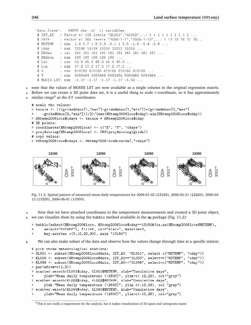
246 Land surface temperature (HRtemp)
'data.frame': 44895 obs. of 11 variables:$ IDT_AK : Factor w/ 123 levels "GL001","GL002",..: 1 1 1 1 1 1 1 1 1 1 ...$ DATE : Factor w/ 365 levels "2006-1-1","2006-1-10",..: 1 12 23 26 27 28...$ MDTEMP : num 1.6 0.7 1.5 0.3 -0.1 1 0.3 -1.9 -5.4 -3.6 ...$ cday : num 13148 13149 13150 13151 13152 ...$ HRdem : int 161 161 161 161 161 161 161 161 161 161 ...$ HRdsea : num 198 198 198 198 198 ...$ Lat : num 45.9 45.9 45.9 45.9 45.9 ...$ Lon : num 17.2 17.2 17.2 17.2 17.2 ...$ X : num 670760 670760 670760 670760 670760 ...$ Y : num 5083464 5083464 5083464 5083464 5083464 ...$ MODIS.LST: num -1.17 -1.17 -1.17 -1.17 -5.92 ...
note that the values of MODIS LST are now available as a single column in the original regression matrix.1
Before we can create a 3D point data set, it is a useful thing to scale t-coordinate, so it has approximately2
similar range6 as the X Y coordinates:3
# scale the values:> tscale <- (((grids@bbox[1,"max"]-grids@bbox[1,"min"])+(grids@bbox[2,"max"]+ -grids@bbox[2,"min"]))/2)/(max(HRtemp2006locs$cday)-min(HRtemp2006locs$cday))> HRtemp2006locs$cdays <- tscale * HRtemp2006locs$cday# 3D points:> coordinates(HRtemp2006locs) <- c("X", "Y", "cdays")> proj4string(HRtemp2006locs) <- CRS(proj4string(grids))# copy values:> HRtemp2006locs$cdays <- HRtemp2006locs@coords[,"cdays"]
13150
●●
●
●●
●
●
●
●
●
●
●
●
●
●
●
●
●
●
●
●
●
●
●
●●●
●
●
●●●
●
●●
●●●
●
●
●
●
●
●
●
●
●
●●
●
●
●
●
●
●
●
●
●
●
●
●
●
●
●
●
●
●
●
●
●●
●
●●
●
●
●
●
●
●
●
●●
●●
●
●
●
●
●●
●●
●
●
●
●
●
●
●
●
●
●
●
●
●
●
●
●
●
●
●
●●
●
●●
●
●●
0102030
13200
●●●
●●
●
●
●
●
●
●
●
●
●
●
●
●
●
●
●
●
●
●
●
●●●
●●
●●●
●
●●
●●●
●
●
●
●●
●
●
●
●
●
●●
●
●
●●
●
●
●
●
●
●
●
●
●
●
●
●
●
●
●
●
●
●●
●
●●
●
●
●
●●
●
●
●●
●●
●
●
●●
●●
●●
●●
●
●
●
●
●
●
●
●
●
●
●
●
●
●
●
●
●●
●
●
●
●●
●
● ●
●
●●
0102030
13250
●●●
●●
●
●
●
●
●
●
●
●
●
●
●●
●
●
●
●
●
●
●
●●●
●●
●●●
●
●●
●●●
●
●
●
●●
●●
●
●
●●
●
●
●●
●
●
●
●
●
●
●
●
●
●
●
●
●
●
●
●
●
●
●●
●
●●
●
●
●●
●
●
●
●●
●●
●
●
●●
●● ●
●●
●
●
●
●
●
●
●
●
●
●
●
●
●
●
●
●●
●
●
●
●●●
● ●
●
●●
0102030
13300
●●●
●●
●
●
●
●
●
●
●
●
●
●
●●
●
●
●
●
●
●
●
●●●
●●
●●●
●
●●
●●●
●
●
●
●●
●
●●
●
●
●●
●
●
●●
●
●
●
●
●
●
●
●
●
●
●
●
●
●
●
●
●
●●
●
●●
●
●
●●
●
●
●●
●●
●●●
●●
● ●
●●
●
●
●
●
●
●
●
●
●
●
●
●
●
●
●
●
●●
●
●
●
●●●
● ●
●
●●
0102030
Fig. 11.2: Spatial pattern of measured mean-daily temperatures for 2006-01-02 (13150), 2006-02-21 (13200), 2006-04-12 (13250), 2006-06-01 (13300).
Now that we have attached coordinates to the temperature measurements and created a 3D point object,4
we can visualize them by using the bubble method available in the sp package (Fig. 11.2):5
> bubble(subset(HRtemp2006locs, HRtemp2006locs$cday==13150&!is.na(HRtemp2006locs$MDTEMP),+ select="MDTEMP"), fill=F, col="black", maxsize=2,+ key.entries=c(0,10,20,30), main="13150")
We can also make subset of the data and observe how the values change through time at a specific station:6
# pick three meteorological stations:> GL001 <- subset(HRtemp2006locs@data, IDT_AK=="GL001", select=c("MDTEMP", "cday"))> KL003 <- subset(HRtemp2006locs@data, IDT_AK=="KL003", select=c("MDTEMP", "cday"))> KL094 <- subset(HRtemp2006locs@data, IDT_AK=="KL094", select=c("MDTEMP", "cday"))> par(mfrow=c(1,3))> scatter.smooth(GL001$cday, GL001$MDTEMP, xlab="Cumulative days",+ ylab="Mean daily temperature (\260C)", ylim=c(-12,28), col="grey")> scatter.smooth(KL003$cday, KL003$MDTEMP, xlab="Cumulative days",+ ylab="Mean daily temperature (\260C)", ylim=c(-12,28), col="grey")> scatter.smooth(KL094$cday, KL094$MDTEMP, xlab="Cumulative days",+ ylab="Mean daily temperature (\260C)", ylim=c(-12,28), col="grey")
6This is not really a requirement for the analysis, but it makes visualization of 3D space and variograms easier.
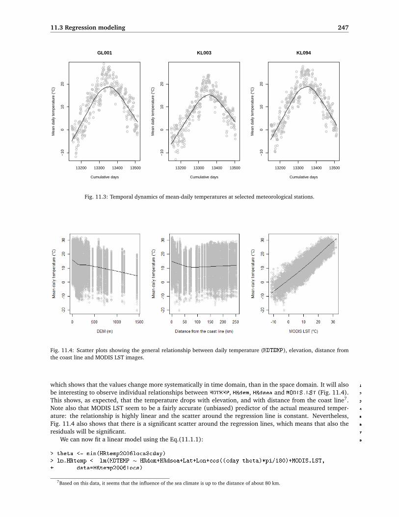
11.3 Regression modeling 247
●●●●●●●
●
●
●●●●●●●●
●
●●
●
●
●
●●
●●
●●
●●
●●●●
●●
●
●●●
●●●
●
●
●●
●●●●
●
●●
●
●●●
●
●
●
●
●●●●
●●●
●
●●
●●●●
●
●
●●
●●
●
●
●
●
●
●●
●
●
●
●
●
●
●
●
●
●
●●●
●●
●
●●●●●●
●●
●
●
●●
●
●
●
●●●
●
●●
●
●
●
●
●
●
●
●
●
●
●
●●
●
●
●
●
●
●●
●
●
●
●●
●
●
●●
●
●
●
●
●
●
●●●
●
●●●●●
●●
●
●
●●
●
●
●●
●●●
●
●
●●
●●●
●●●●
●
●
●
●
●●●●●●●●●
●
●●
●
●
●●
●●●
●
●
●
●
●●●●
●
●
●●●
●
●●
●
●
●●●●
●
●
●●
●●
●●
●●
●●●●●●
●●
●●●●
●●
●
●
●
●●●
●●●●●●
●●●●
●
●●●●●●●
●
●
●●
●
●●
●●
●
●●●
●
●●●
●
●
●
●
●●
●●
●●
●●
●●●●●
●
●●●
●
●
●●
●●●●●●
●
●●
●
●
●
●
●
●
●●●●
●
●
●
●●●●●●
●●
●●
●
●
●
13200 13300 13400 13500
−10
010
20
GL001
Cumulative days
Mea
n da
ily te
mpe
ratu
re (
°C)
●●
●
●●●●●●
●
●●
●
●●
●
●
●
●
●
●
●
●●●
●
●
●●
●●●●
●
●
●●
●
●●
●●●●●
●
●
●●●
●
●●●
●●●
●
●
●
●●
●
●
●●●
●
●
●
●
●●
●
●
●●
●●
●
●
●●
●●●
●
●●
●●
●
●
●
●
●
●
●●
●
●
●●
●
●●
●●
●
●
●●●●●●
●
●
●●
●●●●
●●
●
●●●
●●
●
●●●
●
●
●
●
●
●
●●
●●
●
●
●
●●●
●●●
●●●●●●
●●●●●●●●
●
●
●●
●●
●●●●●●●●
●●
●
●●
●
●
●●●●
●●●
●●
●●●●
●●
●
●●
●●●●●
●
●●
●●
●
●●●
●
●●●
●●
●
●
●
●
●
●
●●
●
●
●●
●
●●●●
●
●●
●●●●
●●●
●●●●●
●●●
●
●●
●
●●●●●●
●●
●●●
●
●
●
●
●●
●●●●
●●
●
●
●●
●
●
●
●
●
●●
●
●
●●●
●
●●●●●●●●
●
●
●
●●
●
●
●
●
●
●●
●
●●●●●
●
●●●
●
●
●●
●
●
●
●
13200 13300 13400 13500
−10
010
20
KL003
Cumulative days
Mea
n da
ily te
mpe
ratu
re (
°C)
●●●●●●●
●
●●●
●●●
●●●
●
●●
●
●
●●●
●●
●
●
●●●●
●●●
●
●
●●
●●●●
●
●
●●
●●
●
●
●●●
●●
●
●
●●
●
●
●
●
●●
●
●●
●
●●
●●●●●
●
●●
●
●
●
●●
●
●
●●
●
●●
●
●
●●
●
●
●
●●●
●
●●●
●●
●●
●●●●
●
●●
●
●●
●
●●●
●●●●●●
●
●●●
●●●●●
●
●
●
●●
●
●●
●
●
●
●
●
●
●●●●
●●
●
●
●●●●
●●
●●●●●
●●●
●●
●
●
●●●●●●
●●●●●
●●●
●
●
●●
●
●
●
●●●●●
●
●●●●●
●
●●
●●
●
●●
●●●
●●
●●
●
●●●
●
●●
●
●
●●●
●
●
●
●●●
●
●●
●●
●
●●●●●
●
●●●●●●●
●●●●●●●●●
●
●●
●
●
●●●●●●●●●●
●
●
●●
●
●●
●●
●●●●●
●
●
●
●
●
●
●
●
●●
●
●●●
●
●●
●●
●
●●●●
●
●
●●
●●●●●
●
●
●
●●●
●●
●
●
●●●●●
●●
●●●●●
●●●
●●
●
●
●
13200 13300 13400 13500
−10
010
20
KL094
Cumulative days
Mea
n da
ily te
mpe
ratu
re (
°C)
Fig. 11.3: Temporal dynamics of mean-daily temperatures at selected meteorological stations.
Fig. 11.4: Scatter plots showing the general relationship between daily temperature (MDTEMP), elevation, distance fromthe coast line and MODIS LST images.
which shows that the values change more systematically in time domain, than in the space domain. It will also 1
be interesting to observe individual relationships between MDTEMP, HRdem, HRdsea and MODIS.LST (Fig. 11.4). 2
This shows, as expected, that the temperature drops with elevation, and with distance from the coast line7. 3
Note also that MODIS LST seem to be a fairly accurate (unbiased) predictor of the actual measured temper- 4
ature: the relationship is highly linear and the scatter around the regression line is constant. Nevertheless, 5
Fig. 11.4 also shows that there is a significant scatter around the regression lines, which means that also the 6
residuals will be significant. 7
We can now fit a linear model using the Eq.(11.1.1): 8
> theta <- min(HRtemp2006locs$cday)> lm.HRtemp <- lm(MDTEMP ∼ HRdem+HRdsea+Lat+Lon+cos((cday-theta)*pi/180)+MODIS.LST,+ data=HRtemp2006locs)
7Based on this data, it seems that the influence of the sea climate is up to the distance of about 80 km.

248 Land surface temperature (HRtemp)
> summary(lm.HRtemp)$adj.r.squared
[1] 0.8423278
# plot(lm.HRtemp)
which shows that all predictors are highly significant; the model explains 84% of variability in the MDTEMP1
values; the derived residuals are normally distributed around the 0 value, with only 3 influential values (out-2
liers).3
11.4 Space-time variogram estimation4
XY
cdays
Fig. 11.5: Cloud plot showing location of meteorological sta-tions in the space-time cube.
Now we can also try to fit the 3D variogram for resid-5
uals. Note that gstat supports 3D interpolation, but6
it does not actually support interactive fitting of 3D7
variograms. In fact, to my knowledge, interactive8
modeling of space-time autocorrelation is still very9
limited in R, but also in commercial packages such10
as Isatis or ArcGIS.11
We can start with plotting the points in a 3D12
space, which is possible by using the cloud method13
available in the lattice package. This will produce a14
plot shown in Fig. 11.5, which gives us a good idea15
about the sampling design specific to this data set.16
The data set consist of large number of space-time17
points. Furthermore, for the purpose of this exer-18
cise, we can first randomly subset the original data19
set to 10% of its size to speed up plotting and fitting20
of the variograms:21
# remove missing values:> HRtemp2006.f <- HRtemp2006locs[-lm.HRtemp$na.action,]# copy the residuals:> HRtemp2006.f$rMDTEMP2006 <- lm.HRtemp$residuals# sub-sample:> HRtemp2006.sel <- HRtemp2006.f[+ runif(length(HRtemp2006.sel$rMDTEMP2006))<0.1,]# str(HRtemp2006.sel)# plot the 3D points:> coords <- as.data.frame(HRtemp2006.sel@coords)> cloud(cdays ∼ X*Y, coords, col="grey")
In addition, assuming that the variogram will be anisotropic, a good idea is to plot a variogram map22
(Fig. 11.6, left):23
> varmap.plt <- plot(variogram(rMDTEMP2006 ∼ 1, HRtemp2006.sel, map=TRUE,+ cutoff=sqrt(areaSpatialGrid(grids))/2, width=30*grids@grid@cellsize[1]),+ col.regions=grey(rev(seq(0,1,0.025))))> rv.MDTEMP2006 <- variogram(rMDTEMP2006 ∼ 1, HRtemp2006.sel, alpha=c(45,135))> rvgm.MDTEMP2006 <- fit.variogram(rv.MDTEMP2006,+ vgm(psill=var(HRtemp2006.sel$rMDTEMP2006),+ "Exp", sqrt(areaSpatialGrid(grids))/4, nugget=0, anis=c(p=45,s=0.5)))> vgm.plt <- plot(rv.MDTEMP2006, rvgm.MDTEMP2006, plot.nu=FALSE, cex=2, pch="+",+ col="black")> print(varmap.plt, split=c(1,1,2,1), more=T)> print(vgm.plt, split=c(2,1,2,1), more=F)> rvgm.MDTEMP2006

11.5 Spatio-temporal interpolation 249
model psill range ang1 anis11 Nug 6.094418 0.00 0 1.02 Exp 4.639634 15392.17 45 0.5
which shows that a strong anisotropy exists (the azimuth of the longer axis is somewhere at 135°), although 1
it is not so distinct. Recall that the main mountain chain on the Balkans (see Fig. 11.1) spreads approximately 2
in the same direction. 3
dx
dy
−2e+05
−1e+05
0e+00
1e+05
2e+05
−2e+05 −1e+05 0e+00 1e+05 2e+05
var1
6
7
8
9
10
11
12
13
14
distance
sem
ivar
ianc
e
2
4
6
8
10
50000 100000 150000 200000
+
++++++++++++++45
50000 100000 150000 200000
+
++++++++++++++
135
Fig. 11.6: Variogram map (left) and fitted anisotropic variogram model (right) for MDTEMP residuals.
The plotted 3D variograms look the same as in Fig. 9.1, although we know that this is not a 2D but a 3D 4
data set. Visual exploration of space-time (3D or 4D) variogram models in R is at the moment limited to 2D 5
spaces, although the situation might change with the new space-time (stpp8) package. Note also from Fig. 11.3 6
that is obvious that nugget variation in time direction will be much higher greater in the space domain. 7
11.5 Spatio-temporal interpolation 8
Making prediction in the space-time domain (3D) is not as easy as making 2D predictions (the previous exer- 9
cises). It will take some time to prepare the prediction locations, get the values of all constant and temporal 10
predictors and then visualize the final results. As mentioned previously, we do not intend to make predictions 11
for the whole space-time cube, but only for fixed time-intervals, i.e. time slices (see also Fig. 2.10). Detailed 12
steps are now explained down-below. 13
11.5.1 A single 3D location 14
We can start by defining the geostatistical model (for residuals): 15
> g.MDTEMP <- gstat(id=c("rMDTEMP2006"), formula=rMDTEMP2006 ∼ 1,+ data=HRtemp2006.f, nmax=40, model=rvgm.MDTEMP2006)
We can now first test the algorithm by using a single 3D point. For example, we ask ourselves what is the 16
mean daily temperature for 1st of August 2006, at location X=575671 E, Y=5083528 N? To prepare the new 17
point location we can use: 18
8http://stpp.r-forge.r-project.org

250 Land surface temperature (HRtemp)
> newloc.t <- "2006-08-01"> newloc.ct <- floor(unclass(as.POSIXct(newloc.t))/86400)[[1]]> newloc.x <- 575671> newloc.y <- 5083528> newloc.xyt <- as.data.frame(matrix(c(newloc.x, newloc.y, tscale*newloc.ct),+ ncol=3, dimnames = list(c("p1"), c("X","Y","cdays"))))> coordinates(newloc.xyt) <- c("X","Y","cdays")> proj4string(newloc.xyt) <- CRS(proj4string(grids))# 3D prediction location:> newloc.xyt
SpatialPoints:X Y cdays
[1,] 575671 5083528 17929560Coordinate Reference System (CRS)arguments: +proj=utm +zone=33+ellps=WGS84 +datum=WGS84 +units=m+no_defs +towgs84=0,0,0
Next, we need to get the values of the auxiliary predictors at this location. We can do this by overlaying1
the new point with the imported gridded maps:2
> newloc.xy <- as.data.frame(newloc.xyt)> coordinates(newloc.xy) <- c("X","Y")> proj4string(newloc.xy) <- CRS(proj4string(grids))> ov.newloc.xy <- overlay(grids, newloc.xy)# add the "time"-location:> ov.newloc.xy$cday <- newloc.ct> str(ov.newloc.xy@data)
'data.frame': 1 obs. of 52 variables:$ HRdem : int 805$ HRdsea : num 165$ Lat : num 45.9$ Lon : num 16$ LST2006_01_01: num NA$ LST2006_01_09: num -5.23...$ LST2006_12_27: num 0.37$ cday : num 13360
Notice that the value of MODIS.LST is missing. The overlay operation works only in 2D, hence it does not3
know what the value of MODIS.LST is for the given date. We need to first estimate what would be the closest4
MODIS image for 2006-08-01, and then copy those values:5
> cdate <- round((unclass(as.POSIXct(newloc.t)) -+ unclass(as.POSIXct("2006-01-01")))/86400, 0)[1]> cdate
[1] 212
> LSTname <- strsplit(LST.listday[which.min(abs(cdate-LSTcdate))], ".LST_")[[1]][1]> LSTname
[1] "LST2006_07_28"
> ov.newloc.xy$MODIS.LST <- ov.newloc.xy@data[,LSTname]> ov.newloc.xy$MODIS.LST
[1] 21.29

11.5 Spatio-temporal interpolation 251
which shows that the ‘closest’ MODIS image is from 2006-07-28 and MODIS estimated temperature for that 1
date is 21.29°C. Now the new location is complete, we can make predict the mean daily temperature at this 2
location, and using the model estimated in the previous section: 3
> locMDTEMP.reg <- predict(lm.HRtemp, ov.newloc.xy)# the trend part:> locMDTEMP.reg
3549718.76291
# OK of residuals;> locMDTEMP <- predict.gstat(g.MDTEMP, newloc.xyt, beta=1, BLUE=FALSE)
[using ordinary kriging]
> locMDTEMP.reg + locMDTEMP$rMDTEMP2006.pred
3549718.98239
which is somewhat lower than we expected for this time of year. Just to check how close the result is to the 4
temperature actually measured at the closest location: 5
# locate the closest measured temperature:> closest.pnt <- which.min(dist(rbind(newloc.xy@coords,+ IDSTA.utm@coords))[1:length(IDSTA.utm@coords[,1])])> closest.IDSTA <- as.character(IDSTA.utm$IDSTA[closest.pnt])> closest.IDSTA
[1] "GL023"
> subset(HRtemp2006locs, HRtemp2006locs$cday==newloc.ct&+ HRtemp2006locs$IDT_AK==closest.IDSTA, select="MDTEMP")
coordinates MDTEMP8243 (575118, 5084260, 17929600) 17.2
which shows that the predicted temperature is somewhat higher than the one measured at the same day, at 6
the closest station. The values are higher mainly because the LST image shows higher values for that period. 7
Surprisingly, the residuals are positive, even though measured values are above predicted and even though the 8
prediction point is fairly close to the measurement location (distance is only 913 m). Take into account that 9
station GL023 is at the top of a mountain, so that it is realistic to always expect a lower temperature even at so 10
short distance. 11
11.5.2 Time-slices 12
We can now generate predictions for a list of new locations. Because there is still no support for 3D grids in R, 13
we can instead make 3D regular points and then predict at those locations. In fact, we will define only slices of 14
the space-time cube for which we will make predictions. Another important issue is that we will put operations 15
in a loop to speed up the processing. Imagine, there are 365 days, and if we would want to interpolate the 16
values for MDTEMP — this would take a lot of scripting. To avoid this problem, we create a R loop that will 17
interpolate as many maps as we like. For the purpose of this exercise, we derive only time-slices for which we 18
also have MODIS images available: 19

252 Land surface temperature (HRtemp)
# available MODIS images:> slices <- LSTdate# new locations:> grids.xy <- as(grids[c("HRdem", "HRdsea", "Lat", "Lon")], "SpatialPixelsDataFrame")> for(i in 1:length(slices)) {> newlocs.xyt <- grids.xy@data> newlocs.xyt$X <- grids.xy@coords[,"x"]> newlocs.xyt$Y <- grids.xy@coords[,"y"]> slice <- floor(unclass(as.POSIXct(slices[i]))/86400)[[1]]> newlocs.xyt$cday <- rep(slice, length(newlocs.xyt[1]))> newlocs.xyt$cdays <- tscale * newlocs.xyt$cday> LSTname <- strsplit(LST.listday[i], ".LST_")[[1]][1]> newlocs.xyt$MODIS.LST <- grids@data[[email protected],LSTname]> coordinates(newlocs.xyt) <- c("X","Y","cdays")> proj4string(newlocs.xyt) <- CRS(proj4string(grids))> MDTEMP.ok <- predict.gstat(g.MDTEMP, newlocs.xyt, beta=1, BLUE=FALSE)> MDTEMP.reg <- predict(lm.HRtemp, newlocs.xyt)> grids@data[,paste(LSTname,".RK",sep="")] <- MDTEMP.reg+MDTEMP.ok$rMDTEMP2006.pred> }
Fig. 11.7: Mean daily temperatures (°C) predicted using spatio-temporal regression-kriging (see titles for dates). Missingpixels are due to clouds in the MODIS LST images.
This operation is relatively time and memory consuming9 so try also to limit the number of slices to <20.1
After the process is finished, a useful thing to do is to visualize the predicted maps together with the measured2
point values by using e.g. (Fig. 11.7):3
> pr.list <- c("LST2006_06_26.RK", "LST2006_07_28.RK", "LST2006_08_29.RK", "LST2006_09_30.RK")> spplot(grids[pr.list], col.regions=grey(seq(0,1,0.025)), at=seq(5,30,1),+ xlim=c(450000,600000), ylim=c(4950000,5100000), sp.layout=list("sp.points",+ IDSTA.utm, pch="+", cex=1.5, col="black"))
You will soon discover that these predictions are mainly controlled by the MODIS LST images (also clearly4
visible from Fig. 11.4); a large portion of NA areas is visible in the output maps. These could be fixed by5
iteratively filtering10 the original MODIS images before these are used as predictors.6
11.5.3 Export to KML: dynamic maps7
We have produced a series of maps of daily temperatures. We want now to export these maps to Google Earth8
and visualize them as a time series. Note that Google Earth support spatio-temporal data that can be browsed9
by using a Timeline bar (Fig. 11.8). In principle, transformation of 2D data to spatio-temporal data is rather10
9A way to speed up the processing would be to limit the search radius (see p.94), but this would also lead to artifacts in the maps.10See for example Addink and Stein (1999).

11.5 Spatio-temporal interpolation 253
simple — we only need to add a field called <TimeSpan> and then define the begin and end time to which a 1
map refers to. If Google Earth sees that this field has been defined, it will automatically browse it with a time 2
slider. We first need to resample all maps to geographic grid (see also section 5.6.2 for more details): 3
# resampling of maps to geographic coordinates:> for(i in seq(5,35,2)) {> LSTname <- strsplit(LST.listday[i], ".LST_")[[1]][1]> write.asciigrid(grids[paste(LSTname, ".RK", sep="")],+ paste(LSTname, "_RK.asc", sep=""), na.value=-999)> rsaga.esri.to.sgrd(in.grids=paste(LSTname, "_RK.asc", sep=""),+ out.sgrd=paste(LSTname, "_RK.sgrd", sep=""), in.path=getwd())# bilinear resample:
> rsaga.geoprocessor(lib="pj_proj4", 2, param=list(SOURCE_PROJ=paste('"',+ proj4string(grids), '"', sep=""), TARGET_PROJ="\"+proj=longlat+ +datum=WGS84\"", SOURCE=paste(LSTname, "_RK.sgrd", sep=""),+ TARGET=paste(LSTname, "_RK_ll.sgrd", sep=""), TARGET_TYPE=0,+ INTERPOLATION=1))# write back to ASCII:
> rsaga.sgrd.to.esri(in.sgrds=paste(LSTname, "_RK_ll.sgrd", sep=""),+ out.grids=paste(LSTname, "_RK.asc", sep=""), prec=1, out.path=getwd())> }
and then read the maps back into R: 4
> MDTEMP.list <- dir(pattern=glob2rx("LST2006_**_**_RK.asc"))> grids.geo <- readGDAL(MDTEMP.list[1])> proj4string(grids.geo) <- CRS("+proj=longlat +datum=WGS84")> names(grids.geo) <- strsplit(MDTEMP.list[1], ".asc")[[1]][1]> for(i in 2:length(MDTEMP.list)){> LSTname <- strsplit(MDTEMP.list[i], ".asc")[[1]][1]> grids.geo@data[,LSTname] <- readGDAL(MDTEMP.list[i])$band1> }
We can now prepare a GE_SpatialGrid object using the original sp SpatialGridDataFrame: 5
> grids.kml <- GE_SpatialGrid(grids.geo)
We want to use the same legend for all time-slices and add it as a screen overlay, which means that we 6
need to determine suitable limits for the legend, e.g. 98% range of values: 7
> MDTEMPxlim <- quantile(HRtemp2006.f$MDTEMP, probs=c(0.01,0.99))> MDTEMPxlim
1% 99%-6.0 28.4
We export all maps as PNGs using a fixed legend: 8
# export all maps as PNG:> for(i in 1:length(MDTEMP.list)) {> LSTname <- strsplit(MDTEMP.list[i], ".asc")[[1]][1]> png(file=paste(LSTname, ".png", sep=""), width=grids.kml$width,+ height=grids.kml$height, bg="transparent")> par(mar=c(0,0,0,0), xaxs="i", yaxs="i")> image(as.image.SpatialGridDataFrame(grids.geo[LSTname]), col=bpy.colors(),+ zlim=(MDTEMPxlim), xlim=grids.kml$xlim, ylim=grids.kml$ylim)> dev.off()> }
To export the legend PNG, we use: 9

254 Land surface temperature (HRtemp)
# prepare the legend:> png(file="legend.png", width=grids.kml$width/4, height=grids.kml$height/3, bg="white")> par(mar=c(0,0.1,0,0.1), yaxs="i")> image(grids, names(grids[5]), col="white")> source("http://spatial-analyst.net/scripts/legend_image.R")> legend_image(c(grids@bbox[1,1],+ grids@bbox[1,2]-(grids@bbox[1,2]-grids@bbox[1,1])/4), c(grids@bbox[2,1],+ grids@bbox[2,2]), seq(MDTEMPxlim[[1]],MDTEMPxlim[[2]],1), vertical=TRUE,+ col=bpy.colors(round(MDTEMPxlim[[2]]-MDTEMPxlim[[1]]/1,0)), offset.leg=.2,+ cex=1.5)> dev.off()
Fig. 11.8: Interpolation of temperatures visualized in Google Earth as time-series of maps. Unlike many standard GIS,Google Earth allows visual exploration of spatio-temporal data. Note from the time-bar that you can also edit the temporalsupport and produce smoothed images in time dimension.
The package maptools does not support export of time-series of maps to Google Earth. This means that1
we need to write the KML file ourselves. This is more simple than you anticipate, because we can again use2
loops (see below). In principle, we only need to respect some common headers and structure used in KML,3
everything else we can easily control. Note also that the KML file structure is easy to read and can be easily4
edited, even manually:5
> filename <- file("MDTEMP2006.kml")> write('<?xml version="1.0" encoding="UTF-8"?>', filename)> write('<kml xmlns="http://earth.google.com/kml/2.2">', filename, append=TRUE)> write('<Folder>', filename, append=TRUE)> write(' <name>Mean Daily TEMP</name>', filename, append=TRUE)> write(' <open>1</open>', filename, append=TRUE)> for(i in 1:length(MDTEMP.list)) {> LSTname <- strsplit(MDTEMP.list[i], ".asc")[[1]][1]# KML is compatible with POSIXct formats:> slice <- as.POSIXct(gsub("_", "-", strsplit(strsplit(MDTEMP.list[i],+ ".asc")[[1]][1], "LST")[[1]][2]))> write(' <GroundOverlay>', filename, append=TRUE)> write(paste(' <name>', LSTname, '</name>',sep=""), filename, append=TRUE)> write(' <TimeSpan>', filename, append=TRUE)

11.6 Summary points 255
> write(paste(' <begin>',slice,'</begin>',sep=""), filename,+ append=TRUE)> write(paste(' <end>',slice+1,'</end>',sep=""), filename, append=TRUE)> write(' </TimeSpan>', filename, append=TRUE)> write(' <color>99ffffff</color>', filename, append=TRUE)> write(' <Icon>', filename, append=TRUE)> write(paste(' <href>', getwd(), '/', LSTname, '.png</href>',sep=""),+ filename, append=TRUE)> write(' <viewBoundScale>0.75</viewBoundScale>', filename,+ append=TRUE)> write(' </Icon>', filename, append=TRUE)> write(' <altitude>50</altitude>', filename, append=TRUE)> write(' <altitudeMode>relativeToGround</altitudeMode>', filename, append=TRUE)> write(' <LatLonBox>', filename, append=TRUE)> write(paste(' <north>',grids.kml$ylim[[2]],'</north>',sep=""),+ filename, append=TRUE)> write(paste(' <south>',grids.kml$ylim[[1]],'</south>',sep=""),+ filename, append=TRUE)> write(paste(' <east>',grids.kml$xlim[[2]],'</east>',sep=""),+ filename, append=TRUE)> write(paste(' <west>',grids.kml$xlim[[1]],'</west>',sep=""),+ filename, append=TRUE)> write(' </LatLonBox>', filename, append=TRUE)> write(' </GroundOverlay>', filename, append=TRUE)> }> write('<ScreenOverlay>', filename, append=TRUE)> write(paste(' <name>from',MDTEMPxlim[[1]],' to+ ',MDTEMPxlim[[2]],'</name>',sep=""), filename, append=TRUE)> write(' <Icon>', filename, append=TRUE)> write(paste(' <href>',getwd(),'/legend.png</href>',sep=""), filename, append=TRUE)> write(' </Icon>', filename, append=TRUE)> write(' <overlayXY x="0" y="0" xunits="fraction" yunits="fraction"/>',+ filename, append=TRUE)> write(' <screenXY x="0" y="0" xunits="fraction" yunits="fraction"/>',+ filename, append=TRUE)> write(' <rotationXY x="0" y="0" xunits="fraction" yunits="fraction"/>',+ filename, append=TRUE)> write(' <size x="0" y="0" xunits="fraction" yunits="fraction"/>',+ filename, append=TRUE)> write(' </ScreenOverlay>', filename, append=TRUE)> write('</Folder>', filename, append=TRUE)> write('</kml>', filename, append=TRUE)> close(filename)
The final output of data export is shown in Fig. 11.8. You can try to modify the original script and produce 1
even more time-slices. In theory, we would normally want to interpolate temperatures for all 365 days and 2
then export all these as images to Google Earth, but this is not maybe a good idea to do considering the size 3
of the maps and the computational effort. 4
11.6 Summary points 5
The results of this case study demonstrate that regression-kriging models can be used also with spatio-temporal 6
records, both of predictors and of target variables. The output pattern of the interpolated temperatures for this 7
data set is mainly controlled with the MODIS LST images. Surprisingly, much of the variation in values can 8
be explained by using just date. On the other hand, local variability of temperatures in the time dimension is 9
more noisy (hence the significant nugget in Fig. 11.6) than in the geographical space. Although elevation and 10
distance from the sea are less significant predictors of temperature than e.g. dates, it is even more important to 11
include information on landscape to model changes in temperatures because this model is based on a physical 12
law. 13

256 Land surface temperature (HRtemp)
This exercises also shows that spatio-temporal prediction models are both more complex and more com-1
putationally intensive than plain spatial techniques. One significant issue not really addressed in this exercise2
is the problem of space-time anisotropy and space-time interactions. One should always address the issue that3
time units principally differ from space units, and separately quantify how fast autocorrelation decreases in4
time, and in space — the differences will often be large (Pebesma et al., 2007). Think of rainfall that might5
occur abruptly over short temporal periods, but then continuously over wide geographical areas. In this ex-6
ercise we have only considered modeling the geometric anisotropy; we have completely ignored products of7
space-time and different scale in time dimension. An alternative would be to model the zonal anisotropy,8
where (also) the variance (sill) depends on direction.9
Estimation of spatio-temporal variograms will often be cumbersome because we need to fit space-time10
models, for which we might not have enough space-time observations (Jost et al., 2005). Not to mention that11
many authors do not believe that temporal variograms are the same in both directions (past vs future). In12
fact, many argue whether there is any logical explanation to use observations from today to predict values13
from yesterday — conceptually speaking, the future does not influence the past! Nevertheless, if you compare14
this approach with the plain 2D techniques used to interpolate daily temperatures (Jarvis and Stuart, 2001;15
Schuurmans et al., 2007), you will notice that the space-time model (Eq.11.1.1) will be able to explain more16
variation in the temperature measurements than e.g. simple ordinary kriging using only temporally fixed17
measurements. Hence it is an investment worth the computational effort.18
Self-study exercises:19
(1.) What is the 95% range of values for MDTEMP? (HINT: use the quantile method and probabilities at 0.02520
and 0.975.)21
(2.) Are the differences between daily values of temperature also very different at other stations? (HINT: try22
looking at least two more stations.)23
(3.) Try to fit a linear model with temperature only. Is the model much different? What would happen if we24
would try to model temperature as a function of time only?25
(4.) How would you decrease the nugget variation in Fig. 11.6? (Consider at least two strategies and then26
try to prove them.)27
(5.) Does it make sense to make predictions of temperature using measurements from a day or more days28
after (the future measurements)? How would you limit the search algorithm to one direction in time29
only?30
(6.) What is the mean daily temperature for 1st of June 2006, at location lon=15.5 E, lat=45.0 N? (HINT:31
you will need to convert the time to numeric variable and then prepare a one-point spatial data layer.32
See section 11.5.1.)33
(7.) At which locations is standard deviation of daily temperatures over the year the highest? (HINT: predict34
MDTEMP values for at least 20 slices over the whole year; then derive the mean value of temperature at35
each grid node and the standard deviation.)36
(8.) Are the maps produced using the method explained in section 11.5.2 valid for the entire mapped region37
or only in the vicinity of the points? (how much are we allowed to extrapolate in geographical space?38
HINT: look at the variogram of residuals in Fig. 11.6.)39
(9.) Obtain temperature measurements for a similar area, download the MODIS LST images (following the40
instructions in §4.2), and repeat this exercise with your own case study.41

11.6 Summary points 257
Further reading: 1
Æ Jarvis, C. H., Stuart, N., 2001. A comparison among strategies for interpolating maximum and minimum 2
daily air temperatures. Part II: The interaction between number of guiding variables and the type of 3
interpolation method. Journal of Applied Meteorology 40: 1075–1084. 4
Æ Jost, G., Heuvelink, G. B. M., Papritz, A. 2005. Analysing the space-time distributions of soil water 5
storage of a forest ecosystem using spatio-temporal kriging. Geoderma 128 (3), 258–273. 6
Æ Huerta, G., Sansó, B., Stroud, J.R. 2004. A spatiotemporal model for Mexico City ozone levels. Journal 7
Of The Royal Statistical Society Series C, 53 (2): 231–248. 8
Æ Pebesma, E. J., de Jong, K., Briggs, D. J., 2007. Visualising uncertain spatial and spatio-temporal data 9
under different scenarios: an air quality example. International Journal of Geographical Information 10
Science 21 (5): 515–527. 11
Æ Schuurmans, J., Bierkens, M., Pebesma, E., Uijlenhoet, R., 2007. Automatic prediction of high-resolution 12
daily rainfall fields for multiple extents: The potential of operational radar. Journal of Hydrometeorology 13
8: 1204–1224. 14

258 Land surface temperature (HRtemp)

Bibliography
Addink, E. A., Stein, A., 1999. A comparison of conventional1
and geostatistical methods to replace clouded pixels in NOAA-2
AVHRR images. International Journal of Remote Sensing 20 (5):3
961–977.4
Ahmed, S., de Marsily, G., 1987. Comparison of geostatistical meth-5
ods for estimating transmissivity using data on transmissivity6
and specific capacity. Water Resources Research 23 (9): 1717–7
1737.8
Amante, C., Eakins, B. W., 2008. ETOPO1 1 Arc-Minute Global9
Relief Model: Procedures, Data Sources and Analysis. National10
Geophysical Data Center, NESDIS, NOAA, U.S. Department of11
Commerce, Boulder, CO, p. 54.12
Araújo, M. B., Thuiller, W., Williams, P. H., Reginster, I., 2005.13
Downscaling european species atlas distributions to a finer res-14
olution: implications for conservation planning. Global Ecology15
and Biogeography 14 (1): 17–30.16
Atkinson, P., Quattrochi, D. A., 2000. Special issue on geostatistics17
and geospatial techniques in remote sensing. Computers & Geo-18
sciences 26 (4): 359.19
Baddeley, A., 2008. Analysing spatial point patterns in R. CSIRO,20
Canberra, Australia, p. 171.21
Bahn, V., McGill, B. J., 2007. Can niche-based distribution models22
outperform spatial interpolation? Global Ecology and Biogeog-23
raphy 16 (6): 733–742.24
Bailey, N., Clements, T., Lee, J. T., Thompson, S., 2003. Modelling25
soil series data to facilitate targeted habitat restoration: a poly-26
tomous logistic regression approach. Journal of Environmental27
Management 67 (4): 395–407.28
Banerjee, S., Carlin, C. P., Gelfand, A. E. (Eds.), 2004. Hierarchical29
Modeling and Analysis for Spatial Data. Monographs on Statis-30
tics and Applied Probability. Chapman & Hall/CRC, Boca Raton,31
Florida, p. 472.32
Banks, J. (Ed.), 1998. Handbook of Simulation — Principles,33
Methodology, Advances, Applications, and Practice. Wiley, New34
York, p. 864.35
Bárdossy, A., Li, J., 2008. Geostatistical interpolation using copulas.36
Water Resources Research 44: W07412.37
Bartholome at al., 2002. GLC 2000 Global Land Cover mapping for38
the year 2000. EUR 20524 EN. European Commission, DG Joint39
Research Centre, Luxemburg, p. 62.40
Batjes, N., 1996. Total carbon and nitrogen in the soils of the world. 41
European Journal of Soil Science 47: 151–163. 42
Batjes, N., 2008. ISRIC-WISE Harmonized Global Soil Profile 43
Dataset (Ver. 3.1). Report 2008/02 (with dataset). ISRIC — 44
World Soil Information, Wageningen, p. 59. 45
Batjes, N., 2009. Harmonized soil profile data for applications at 46
global and continental scales: updates to the WISE database. 47
Soil Use and Management 25: 124–127. 48
Batjes, N., Al-Adamat, R., Bhattacharyya, T., Bernoux, M., Cerri, 49
C., Gicheru, P., Kamoni, P., Milne, E., Pal, D., Rawajfi, Z., 2007. 50
Preparation of consistent soil data sets for modelling purposes: 51
Secondary SOTER data for four case study areas. Agriculture, 52
Ecosystems & Environment 122: 26–34. 53
Becker, J. J., Sandwell, D. T., Smith, W. H. F., Braud, J., Binder, B., 54
Depner, J., Fabre, D., Factor, J., Ingalls, S., Kim, S.-H., Ladner, 55
R., Marks, K., Nelson, S., Pharaoh, A., Sharman, G., Trimmer, 56
R., vonRosenburg, J., Wallace, G., Weatherall, P., 2009. Global 57
Bathymetry and Elevation Data at 30 Arc Seconds Resolution: 58
SRTM30_PLUS. Marine Geodesy in press: 18. 59
Berman, M., Diggle, P. J., 1989. Estimating weighted integrals of 60
the second-order intensity of a spatial point process. Journal of 61
the Royal Statistical Society B 51: 81–92. 62
Bierkens, M. F. P., Burrough, P. A., 1993. The indicator approach to 63
categorical soil data I: Theory. Journal of Soil Science 44: 361– 64
368. 65
Bishop, T., Minasny, B., McBratney, A., 2006. Uncertainty analysis 66
for soil-terrain models. International Journal of Geographical In- 67
formation Science 20 (1-2): 117–134. 68
Bishop, T. F. A., McBratney, A. B., 2001. A comparison of predic- 69
tion methods for the creation of field-extent soil property maps. 70
Geoderma 103 (1-2): 149–160. 71
Bishop, T. F. A., Minasny, B., 2005. Digital Soil-Terrain Modelling: 72
The Predictive Potential and Uncertainty. In: Grunwald, S. (Ed.), 73
Environmental Soil-Landscape Modeling: Geographic Informa- 74
tion Technologies and Pedometrics. CRC Press, Boca Raton, 75
Florida, pp. 185–213. 76
Bivand, R., 2006. Implementing Spatial Data Analysis Software 77
Tools in R. Geographical Analysis 38: 23–40. 78
Bivand, R., Pebesma, E., Rubio, V., 2008. Applied Spatial Data Anal- 79
ysis with R. Use R Series. Springer, Heidelberg, p. 400. 80
259

260 Bibliography
Bivand, R. S., 2005. Interfacing GRASS 6 and R. Status and devel-1
opment directions. GRASS Newsletter 3: 11–16.2
Bleines, C., Perseval, S., Rambert, F., Renard, D., Touffait, Y., 2004.3
ISATIS. Isatis software manual, 5th Edition. Geovariances &4
Ecole Des Mines De, Paris, p. 710.5
Bolstad, P. (Ed.), 2008. GIS Fundamentals, 3rd Edition. Atlas Books,6
Minnesota, p. 650.7
Bonan, G. B., Levis, S., Sitch, S., Vertenstein, M., Oleson, K. W.,8
2003. A dynamic global vegetation model for use with climate9
models: concepts and description of simulated vegetation dy-10
namics. Global Change Biology 9 (11): 1543–1566.11
Boucneau, G., van Meirvenne, M., Thas, O., Hofman, G., 1998. Inte-12
grating properties of soil map delineations into ordinary kriging.13
European Journal of Soil Science 49 (2): 213–229.14
Box, G. E. P., Muller, M. E., 1958. A note on the generation of15
random normal deviates. The Annals of Mathematical Statistics16
29 (2): 610–611.17
Bragato, G., 2004. Fuzzy continuous classification and spatial in-18
terpolation in conventional soil survey for soil mapping of the19
lower Piave plain. Geoderma 118 (1-2): 1–16.20
Brenning, A., 2008. Statistical geocomputing combining r and saga:21
The example of landslide susceptibility analysis with generalized22
additive models. In: Böhner, J., Blaschke, T., Montanarella, L.23
(Eds.), SAGA — Seconds Out. Vol. 19. Hamburger Beiträge zur24
Physischen Geographie und Landschaftsökologie, pp. 23–32.25
Brus, D. J., Heuvelink, G. B. M., 2007. Optimization of sample pat-26
terns for universal kriging of environmental variables. Geoderma27
138 (1-2): 86–95.28
Burns, P., 2009. The R Inferno. Burns Statistics, London, p. 103.29
Burrough, P. A., McDonnell, R. A., 1998. Principles of Geographical30
Information Systems. Oxford University Press Inc., New York, p.31
333.32
Calenge, C., 2007. Exploring Habitat Selection by Wildlife with ade-33
habitat. Journal of Statistical Software 22 (6): 2–19.34
Carré, F., Girard, M. C., 2002. Quantitative mapping of soil types35
based on regression kriging of taxonomic distances with land-36
form and land cover attributes. Geoderma 110 (3-4): 241–263.37
Chambers, J. M., Hastie, T. J., 1992. Statistical Models in S.38
Wadsworth & Brooks/Cole, Pacific Grove, California, p. 595.39
Chang Seong, J., Mulcahy, K., Usery, E., 2002. The Sinusoidal Pro-40
jection: A New Importance in Relation to Global Image Data.41
The Professional Geographer 54 (2): 218–225.42
Chefaoui, R. M., Lobo, J. M., 2008. Assessing the effects of pseudo-43
absences on predictive distribution model performance. Ecolog-44
ical Modelling 210: 478–486.45
Chiles, J. P., Delfiner, P., 1999. Geostatistics: modeling spatial un-46
certainty. John Wiley & Sons, New York, p. 720.47
Christensen, R., 2001. Linear Models for Multivariate, Time Series,48
and Spatial Data, 2nd Edition. Springer Verlag, New York, p. 393.49
Congalton, R. G., Green, K., 1999. Assessing the accuracy of re-50
motely sensed data: principles and practices. Lewis, Boca Raton,51
FL, p. 137.52
Conrad, O., 2006. SAGA — Program Structure and Current State of53
Implementation. In: Böhner, J., McCloy, K. R., Strobl, J. (Eds.),54
SAGA — Analysis and Modelling Applications. Vol. 115. Verlag55
Erich Goltze GmbH, pp. 39–52.56
Conrad, O., 2007. SAGA — Entwurf, Funktionsumfang und An- 57
wendung eines Systems für Automatisierte Geowissenschaftliche 58
Analysen. Ph.D. thesis, University of Göttingen, Göttingen. 59
Craglia, M., Goodchild, M., Annoni, A., Camara, G., Gould, M., 60
Kuhn, W., Mark, D., Masser, I., Maguire, D., Liang, S., Parsons, 61
E., 2008. Next-Generation Digital Earth: A position paper from 62
the Vespucci Initiative for the Advancement of Geographic Infor- 63
mation Science. International Journal of Spatial Data Infrastruc- 64
tures Research 3 (6): 146–167. 65
Cressie, N. A. C., 1990. The origins of kriging. Mathematical Geol- 66
ogy 22 (3): 239–252. 67
Cressie, N. A. C., 1993. Statistics for Spatial Data, revised edition. 68
John Wiley & Sons, New York, p. 416. 69
D’Agostino, V., Zelenka, A., 1992. Supplementing solar radiation 70
network data by co-Kriging with satellite images. International 71
Journal of Climatology 12 (7): 749–761. 72
Davis, C., Fonseca, F., Câmara, G., 2009. Beyond SDI: Integrating 73
Science and Communities to Create Environmental Policies for 74
the Sustainability of the Amazon. International Journal of Spa- 75
tial Data Infrastructures Research 4: 156–174. 76
de Fries, F., Groot, W., Hoogland, T., Denneboom, J., 2003. De 77
Bodemkaart van Nederland digitaal. Alterra Rapport 811. Al- 78
terra, Wageningen, p. 45. 79
de Gruijter, J. J., Walvoort, D. J. J., van Gaans, P. F. M., 1997. Contin- 80
uous soil maps — a fuzzy set approach to bridge the gap between 81
aggregation levels of process and distribution models. Geoderma 82
77 (2-4): 169–195. 83
Deutsch, C. V., Journel, A. G., 1998. GSLIB: Geostatistical Software 84
and User’s Guide, 2nd Edition. Oxford University Press, New 85
York, p. 384. 86
Dial, G., Bowen, H., Gerlach, F., Grodecki, J., Oleszczuk, R., 2003. 87
Ikonos satellite, imagery, and products. Remote Sensing of Envi- 88
ronment 88: 23–36. 89
Diggle, P. J., 2003. Statistical Analysis of Spatial Point Patterns, 2nd 90
Edition. Arnold Publishers, p. 288. 91
Diggle, P. J., Ribeiro Jr, P. J., 2007. Model-based Geostatistics. 92
Springer Series in Statistics. Springer, p. 288. 93
Doll, C., Muller, J.-P., Morley, J., 2007. Mapping regional economic 94
activity from night-time light satellite imagery. Ecological Eco- 95
nomics 57 (1): 75–92. 96
Donato, G., Belongie, S., 2003. Approximation Methods for Thin 97
Plate Spline Mappings and Principal Warps. In: Heyden, A., 98
Sparr, G., Nielsen, M., Johansen, P. (Eds.), Proceedings, Part III, 99
Lecture Notes in Computer Science. Computer Vision — ECCV 100
2002: 7th European Conference on Computer Vision. Copen- 101
hagen, Denmark, pp. 21–31. 102
Dooley, M. A., Lavin, S. J., 2007. Visualizing method-produced un- 103
certainty in isometric mapping. Cartographic Perspectives 56: 104
17–36. 105
D’Or, D., 2003. Spatial prediction of soil properties, the Bayesian 106
Maximum Entropy approach. Phd, Université Catholique de Lou- 107
vain. 108
D’Or, D., Bogaert, P., 2005. Spatial prediction of categorical vari- 109
ables with the Bayesian Maximum Entropy approach: the Ooy- 110
polder case study. European Journal of Soil Science 55 (Decem- 111
ber): 763–775. 112
Draper, N. R., Smith, H., 1998. Applied Regression Analysis, 3rd 113
Edition. John Wiley, New York, p. 697. 114

Bibliography 261
Dubois, G. (Ed.), 2005. Automatic mapping algorithms for routine1
and emergency monitoring data. Report on the Spatial Interpo-2
lation Comparison (SIC2004) exercise. EUR 21595 EN. Office3
for Official Publications of the European Communities, Luxem-4
bourg, p. 150.5
Dubois, G., Galmarini, S., 2004. Introduction to the Spatial Inter-6
polation Comparison (SIC). Applied GIS 1 (2): 9–11.7
Ellis, E., Ramankutty, N., 2000. Putting people in the map: an-8
thropogenic biomes of the world. Frontiers in Ecology and the9
Environment 6 (8): 439–447.10
Endreny, T. A., Wood, E. F., 2001. Representing elevation uncer-11
tainty in runoff modelling and flowpath mapping. Hydrological12
Processes 15: 2223–2236.13
Engler, R., Guisan, A., Rechsteiner, L., 2004. An improved approach14
for predicting the distribution of rare and endangered species15
from occurrence and pseudo-absence data. Journal of Applied16
Ecology 41 (2): 263–274.17
Eswaran, H., van den Berg, E., Reich, P., 1993. Organic carbon in18
soils of the world. Soil Science Society of America journal 57:19
192–194.20
Evans, J. S., Hudak, A. T., 2007. A multiscale curvature filter for21
identifying ground returns from discrete return lidar in forested22
environments. IEEE Transactions on Geoscience and Remote23
Sensing 45 (4): 1029–1038.24
Fassó, A., Cameletti, M., 2009. A Unified Statistical Approach for25
Simulation, Modeling, Analysis and Mapping of Environmental26
Data. SIMULATION in press: 1–16.27
Fisher, P., 1998. Improved Modeling of Elevation Error with Geo-28
statistics. GeoInformatica 2 (3): 215–233.29
Fisher, P. F., Wood, J., Cheng, T., 2005. Fuzziness and Ambiguity30
in Multi-Scale Analysis of Landscape Morphometry. In: Petry,31
F. E., Robinson, V. B., Cobb, M. A. (Eds.), Fuzzy Modeling with32
Spatial Information for Geographic Problems. Springer-Verlag,33
Berlin, pp. 209–232.34
Foody, G. M., 2004. Thematic map comparison: evaluating the sta-35
tistical significance of differences. Photogrammetric Engineering36
and Remote Sensing 70: 627–633.37
Fotheringham, A. S., Brunsdon, C., Charlton, M., 2002. Geographi-38
cally Weighted Regression: The Analysis of Spatially Varying Re-39
lationships. GIS & Remote Sensing. Wiley, p. 282.40
Gandin, L. S., 1963. Objective Analysis of Meteorological Fields.41
translated from Russian in 1965 by Israel Program for Scientific42
Translations, Jerusalem. Gidrometeorologicheskoe Izdatel’stvo43
(GIMIZ), Leningrad, p. 242.44
Gelfand, A. E., Kim, H.-J., Sirmans, C. F., , Banerjee, S., 2003. Spa-45
tial Modeling With Spatially Varying Coefficient Processes. Jour-46
nal of the American Statistical Association 98 (462): 387–396.47
Goldberger, A., 1962. Best Linear Unbiased Prediction in the Gen-48
eralized Linear Regression Model. Journal of the American Sta-49
tistical Association 57: 369–375.50
Goovaerts, P., 1997. Geostatistics for Natural Resources Evaluation51
(Applied Geostatistics). Oxford University Press, New York, p.52
496.53
Goovaerts, P., 1999. Geostatistics in soil science: State-of-the-art54
and perspectives. Geoderma 89 (1-2): 1–45.55
Gotway, C., Young, L., 2002. Combining Incompatible Spatial Data.56
Journal of the American Statistical Association 97: 632–648.57
Gotway, C. A., Stroup, W. W., 1997. A Generalized Linear Model ap- 58
proach to spatial data analysis and prediction. Journal of Agri- 59
cultural, Biological, and Environmental Statistics 2 (2): 157– 60
198. 61
Gotway Crawford, C. A., Young, L. J., 2008. Geostatistics: What’s 62
Hot, What’s Not, and Other Food for Thought. In: Wan, Y. et al. 63
(Ed.), Proceeding of the 8th international symposium on spatial 64
accuracy assessment in natural resources and environmental sci- 65
ences (Accuracy 2008). World Academic Union (Press), Shang- 66
hai, pp. 8–16. 67
Griffith, D., 2008. Spatial-filtering-based contributions to a critique 68
of geographically weighted regression (GWR). Environment and 69
Planning A40: 2751–2769. 70
Grohmann, C. H., 2004. Morphometric analysis in Geographic In- 71
formation Systems: applications of free software GRASS and R. 72
Computers & Geosciences 30: 1055–1067. 73
Groombridge, B., Jenkins, M., 2002. World Atlas of Biodiversity: 74
Earth’s Living Resources in the 21st Century. University of Cali- 75
fornia Press, p. 340. 76
Grose, D., Crouchley, R., van Ark, T., Allan, R., Kewley, J., Braimah, 77
A., Hayes, M., 2006. sabreR: Grid-Enabling the Analysis of Mul- 78
tiProcess Random Effect Response Data in R. In: Halfpenny, 79
P. (Ed.), Second International Conference on e-Social Science. 80
Vol. 3c. National Centre for e-Social Science, Manchester, UK, 81
p. 12. 82
Grossman, J., Grosz, A., Schweitzer, P., Schruben, P. (Eds.), 2008. 83
The National Geochemical Survey — Database and Documen- 84
tation, Version 5. Open-File Report 2004-1001. U.S. Geological 85
Survey, Reston, VA, p. 45. 86
Guisan, A., Zimmermann, N. E., 2000. Predictive habitat distribu- 87
tion models in ecology. Ecological Modelling 135 (2-3): 147– 88
186. 89
Guttorp, P., 2003. Environmental Statistics — A Personal View. In- 90
ternational Statistical Review 71: 169–179. 91
Haas, T. C., 1990. Kriging and automated semivariogram modelling 92
within a moving window. Atmospheric Environment 24A: 1759– 93
1769. 94
Hansen, M., DeFries, R., Townshend, J., Sohlberg, R., 2000. Global 95
land cover classification at 1km resolution using a decision tree 96
classifier. International Journal of Remote Sensing 21: 1331– 97
1365. 98
Hardy, R. L., 1971. Multiquadratic equations of topography and 99
other irregular surfaces. Journal of Geophysical Research 76: 100
1905–1915. 101
Hayakawa, Y., Oguchi, T., Lin, Z., 2008. Comparison of new and ex- 102
isting global digital elevation models: ASTER G-DEM and SRTM- 103
3. Geophys. Res. Lett. 35: L17404. 104
Henderson, B. L., Bui, E. N., Moran, C. J., Simon, D. A. P., 2004. 105
Australia-wide predictions of soil properties using decision trees. 106
Geoderma 124 (3-4): 383–398. 107
Hengl, T., 2006. Finding the right pixel size. Computers & Geo- 108
sciences 32 (9): 1283–1298. 109
Hengl, T., Bajat, B., Reuter, H., Blagojevic, D., 2008. Geostatisti- 110
cal modelling of topography using auxiliary maps. Computers & 111
Geosciences 34: 1886–1899. 112
Hengl, T., Heuvelink, G. B. M., Rossiter, D. G., 2007a. About 113
regression-kriging: from theory to interpretation of results. Com- 114
puters & Geosciences 33 (10): 1301–1315. 115

262 Bibliography
Hengl, T., Heuvelink, G. M. B., Stein, A., 2004a. A generic frame-1
work for spatial prediction of soil variables based on regression-2
kriging. Geoderma 122 (1-2): 75–93.3
Hengl, T., Minasny, B., Gould, M., 2009a. A geostatistical analysis4
of geostatistics. Scientometrics 80: 491–514.5
Hengl, T., Reuter, H. (Eds.), 2008. Geomorphometry: Concepts,6
Software, Applications. Vol. 33 of Developments in Soil Science.7
Elsevier, Amsterdam, p. 772.8
Hengl, T., Rossiter, D. G., Stein, A., 2004b. Soil sampling strategies9
for spatial prediction by correlation with auxiliary maps. Aus-10
tralian Journal of Soil Research 41 (8): 1403–1422.11
Hengl, T., Sierdsema, H., Radovic, A., Dilo, A., 2009b. Spatial pre-12
diction of species’ distributions from occurrence-only records:13
combining point pattern analysis, ENFA and regression-kriging.14
Ecological Modelling 220: 3499–3511.15
Hengl, T., Toomanian, N., 2006. Maps are not what they seem:16
representing uncertainty in soil-property maps. In: Caetano, M.,17
Painho, M. (Eds.), Proceedings of the 7th International Sympo-18
sium on Spatial Accuracy Assessment in Natural Resources and19
Environmental Sciences (Accuracy 2006). Instituto Geográphico20
Português, Lisbon, Portugal, pp. 805–813.21
Hengl, T., Toomanian, N., Reuter, H. I., Malakouti, M. J., 2007b.22
Methods to interpolate soil categorical variables from profile ob-23
servations: lessons from Iran. Geoderma 140 (4): 417–427.24
Hengl, T., Walvoort, D. J. J., Brown, A., Rossiter, D. G., 2004c. A25
double continuous approach to visualisation and analysis of cate-26
gorical maps. International Journal of Geographical Information27
Science 18 (2): 183–202.28
Hession, S. L., Shortridge, A. M., Torbick, M. N., 2006. Categorical29
models for spatial data uncertainty. In: Caetano, M., Painho, M.30
(Eds.), Proceedings of the 7th International Symposium on Spa-31
tial Accuracy Assessment in Natural Resources and Environmen-32
tal Sciences (Accuracy 2006). Instituto Geográphico Português,33
Lisbon, pp. 386–395.34
Heuvelink, G., 1998. Error propagation in environmental modelling35
with GIS. Taylor & Francis, London, UK, p. 144.36
Heuvelink, G., 2002. Analysing uncertainty propagation in GIS:37
why is it not that simple? In: Foody, G., Atkinson, P. (Eds.),38
Uncertainty in Remote Sensing and GIS. Wiley, Chichester, pp.39
155–165.40
Heuvelink, G. B. M., Pebesma, E. J., 1999. Spatial aggregation and41
soil process modelling. Geoderma 89 (1-2): 47–65.42
Heuvelink, G. B. M., Webster, R., 2001. Modelling soil variation:43
past, present, and future. Geoderma 100 (3-4): 269–301.44
Hijmans, R., Cameron, S., Parra, J., Jones, P., Jarvis, A., 2005. Very45
high resolution interpolated climate surfaces for global land ar-46
eas. International Journal of Climatology 25: 1965–1978.47
Hirzel, A. H., Guisan, A., 2002. Which is the optimal sampling48
strategy for habitat suitability modelling. Ecological Modelling49
157 (2-3): 331–341.50
Holmes, K. W., Chadwick, O. A., Kyriakidis, P. C., 2000. Error in51
a USGS 30m digital elevation model and its impact on digital52
terrain modeling. Journal of Hydrology 233: 154–173.53
Hsing-Cheng, H., Chun-Shu, C., 2007. Optimal Geostatistical Model54
Selection. Journal of the American Statistical Association 102:55
1009–1024.56
Huerta, G., Sansó, B., Stroud, J., 2004. A spatiotemporal model 57
for Mexico City ozone levels. Journal Of The Royal Statistical 58
Society Series C 53 (2): 231–248. 59
Huete, A., Didan, K., Miura, T., Rodriguez, E., Gao, X., Ferreira, L., 60
2002. Overview of the radiometric and biophysical performance 61
of the MODIS vegetation indices. Remote Sensing of Environ- 62
ment 83: 195–213. 63
Hunter, G. J., Goodchild, M. F., 1997. Modeling the Uncertainty 64
of Slope and Aspect Estimates Derived from Spatial Databases. 65
Geographical Analysis 29 (1): 35–49. 66
Hutchinson, M. F., 1989. A new procedure for gridding elevation 67
and stream line data with automatic removal of spurious pits. 68
Journal of Hydrology 106: 211–232. 69
Hutchinson, M. F., 1995. Interpolating mean rainfall using thin 70
plate smoothing splines. International Journal of Geographical 71
Information Systems 9: 385–403. 72
Hutchinson, M. F., 1996. A locally adaptive approach to the interpo- 73
lation of digital elevation models. In: Proceedings of the Third 74
International Conference/Workshop on Integrating GIS and En- 75
vironmental Modeling. National Center for Geographic Informa- 76
tion and Analysis, Santa Barbara, CA, p. 6. 77
Isaaks, E. H., Srivastava, R. M., 1989. Applied Geostatistics. Oxford 78
University Press, New York, p. 542. 79
Jarvis, C. H., Stuart, N., 2001. A comparison among strategies for 80
interpolating maximum and minimum daily air temperatures. 81
Part II: The interaction between number of guiding variables and 82
the type of interpolation method. Journal of Applied Meteorol- 83
ogy 40: 1075–1084. 84
Jiménez-Valverde, A., Gómez, J., Lobo, J., Baselga, A., Hortal, J., 85
2008. Challenging species distribution models: the case of Ma- 86
culinea nausithous in the Iberian Peninsula. Annales Zoologici 87
Fennici 45: 200–210. 88
Jost, G., Heuvelink, G. B. M., Papritz, A., 2005. Analysing the space- 89
time distributions of soil water storage of a forest ecosystem us- 90
ing spatio-temporal kriging. Geoderma 128 (3): 258–273. 91
Journel, A. G., 1986. Constrained interpolation and qualitative in- 92
formation. Mathematical Geology 18 (3): 269–286. 93
Kanevski, M., Maignan, M., Demyanov, V., Maignan, M., 1997. 94
How neural network 2-D interpolations can improve spatial data 95
analysis: neural network residual kriging (NNRK). In: Hohn, 96
M. (Ed.), Proceedings of the Third Annual Conference of the 97
IAMG. International Center for Numerical Methods in Engineer- 98
ing (CIMNE), Barcelona, Spain, pp. 549–554. 99
Kempen, B., Brus, D., Heuvelink, G., Stoorvogel, J., 2009. Updating 100
the 1:50,000 Dutch soil map using legacy soil data: A multino- 101
mial logistic regression approach. Geoderma 151 (3-4): 311– 102
326. 103
Kitanidis, P. K., 1994. Generalized covariance functions in estima- 104
tion. Mathematical Geology 25: 525–540. 105
Kleinschmidt, I. Sharp, B. L., Clarke, G. P. Y., Curtis, B., Fraser, C., 106
2005. Use of Generalized Linear Mixed Models in the Spatial 107
Analysis of Small-Area Malaria Incidence Rates in KwaZulu Na- 108
tal, South Africa. American Journal of Epidemiology 153 (12): 109
1213–1221. 110
Knotters, M., Brus, D. J., Voshaar, J. H. O., 1995. A comparison of 111
kriging, co-kriging and kriging combined with regression for spa- 112
tial interpolation of horizon depth with censored observations. 113
Geoderma 67 (3-4): 227–246. 114

Bibliography 263
Koptsik, S., Koptsik, G., Livantsova, S., Eruslankina, L., Zhmelkova,1
T., Vologdina, Z., 2003. Heavy metals in soils near the nickel2
smelter: Chemistry, spatial variation, and impacts on plant di-3
versity. Journal of Environmental Monitoring 5 (3): 441–50.4
Kreft, H., Jetz, W., 2007. Global Patterns and Determinants of Vas-5
cular Plant Diversity. Proceedings National Academy of Science6
104: 5925–5930.7
Krige, D. G., 1951. A statistical approach to some basic mine valu-8
ation problems on the Witwatersrand. Journal of the Chemical,9
Metallurgical and Mining Society 52: 119–139.10
Kuhnert, P., Venables, W. N., 2005. An Introduction to R: Software11
for Statistical Modelling & Computing. CSIRO, Canberra, Aus-12
tralia, p. 362.13
Kutner, M. H., Nachtsheim, C. J., Neter, J., Li, W. (Eds.), 2004.14
Applied Linear Statistical Models, 5th Edition. McGraw-Hill, p.15
1396.16
Kyriakidis, P. C., Journel, A. G., 1999. Geostatistical Space–Time17
Models: A Review. Mathematical Geology 31 (6): 651–684.18
Kyriakidis, P. C., Shortridge, A. M., Goodchild, M. F., 1999. Geo-19
statistics for conflation and accuracy assessment of Digital Eleva-20
tion Models. International Journal of Geographical Information21
Science 13 (7): 677–708.22
Lagacherie, P., McBratney, A., Voltz, M. (Eds.), 2006. Digital Soil23
Mapping: An Introductory Perspective. Developments in Soil Sci-24
ence. Elsevier, Amsterdam, p. 350.25
Lam, N. S.-N., 1983. Spatial interpolation methods: a review. The26
American Cartographer 10: 129–149.27
Lark, R. M., Cullis, B., Welham, S. J., 2005. On Spatial Prediction of28
Soil Properties in the Presence of a Spatial Trend: The Empirical29
Best Linear Unbiased Predictor (E-BLUP) with REML. European30
Journal of Soil Science 57: 787–799.31
Latimer, A. M., Wu, S., Gelfand, A. E., Silander Jr., J. A., 2004.32
Building statistical models to analyze species distributions. Eco-33
logical Applications 16 (1): 33–50.34
Legendre, P., Fortin, M. J., 1989. Spatial pattern and ecological anal-35
ysis. Plant Ecology 80 (2): 107–138.36
Lehner, B., Doll, P., 2004. Development and validation of a global37
database of lakes, reservoirs and wetlands. Journal of Hydrology38
296 (1-4): 1–22.39
Leigh, E. G. J., de Lao, S. L., Condit, R. G., Hubbell, S. P., Foster,40
R. B., Perez, R., 2004. Barro Colorado Island Forest Dynamics41
Plot, Panama. In: Losos, E. C., Leigh, E. G. J. (Eds.), Tropical42
forest diversity and dynamism: Findings from a large-scale plot43
network. University of Chicago Press, Chicago, pp. 451–463.44
Leopold, U., Heuvelink, G. B. M., Tiktak, A., Finke, P. A.,45
Schoumans, O., 2005. Accounting for change of support in spa-46
tial accuracy assessment of modelled soil mineral phosphorous47
concentration. Geoderma 130 (3-4): 368–386.48
Li, J., Heap, A., 2008. A review of spatial interpolation methods for49
environmental scientists. Record 2008/23. Geoscience Australia,50
Canberra, p. 137.51
Li, W., Zhang, C., Burt, J., Zhu, A., 2005a. A markov chain-based52
probability vector approach for modelling spatial uncertainties53
of soil classes. Soil Science Society of America Journal 69: 1931–54
1942.55
Li, W., Zhang, C., Burt, J., Zhu, A., Feyen, J., 2004. Two-dimensional56
markov chain simulation of soil type spatial distribution. Soil57
Science Society of America Journal 68: 1479–1490.58
Li, Z., Zhu, Q., Gold, C., 2005b. Digital Terrain Modeling: Principles 59
and Methodology. CRC Press, Boca Raton, Florida, p. 319. 60
Lloyd, C., 2009. Nonstationary models for exploring and map- 61
ping monthly precipitation in the United Kingdom. International 62
Journal of Climatology in press. 63
Lloyd, C. D., 2005. Assessing the effect of integrating elevation data 64
into the estimation of monthly precipitation in Great Britain. 65
Journal of Hydrology 308 (1-4): 128–150. 66
Lloyd, C. D., Atkinson, P. M., 1998. Scale and the spatial structure of 67
landform: optimizing sampling strategies with geostatistics. In: 68
Proceedings of the 3rd International Conference on GeoCompu- 69
tation, University of Bristol, United Kingdom, 17-19 September 70
1998. University of Bristol, Bristol, UK, p. 16. 71
Lloyd, C. D., Atkinson, P. M., 2002. Deriving DSMs from LiDAR data 72
with kriging. International Journal of Remote Sensing 23 (12): 73
2519–2524. 74
Lunetta, R., Knight, J., Ediriwickrema, J., Lyon, J., Dorsey Wor- 75
thy, L., 2006. Land-cover change detection using multi-temporal 76
MODIS NDVI data. Remote Sensing of Environment 105 (2): 77
142–154. 78
Matheron, G., 1962. Traité de géostatistique appliquée. Vol. 14 of 79
Mémoires du Bureau de Recherches Géologiques et Minières. 80
Editions Technip, Paris, p. NA. 81
Matheron, G., 1969. Le krigeage universel. Vol. 1. Cahiers du Cen- 82
tre de Morphologie Mathématique, École des Mines de Paris, 83
Fontainebleau, p. NA. 84
McBratney, A. B., de Gruijter, J. J., Brus, D. J., 1992. Spatial predic- 85
tion and mapping of continuous soil classes. Geoderma 54 (1-4): 86
39–64. 87
McBratney, A. B., Mendoça Santos, M. L., Minasny, B., 2003. On 88
digital soil mapping. Geoderma 117 (1-2): 3–52. 89
McCloskey, J., Spalding, H., 1989. A reconnaissance level inven- 90
tory of the amount of wilderness remaining in the world. Ambio 91
18 (4): 221–227. 92
McKenzie, N. J., Ryan, P. J., 1999. Spatial prediction of soil prop- 93
erties using environmental correlation. Geoderma 89 (1-2): 67– 94
94. 95
Miller, J., 2005. Incorporating Spatial Dependence in Predictive 96
Vegetation Models: Residual Interpolation Methods. The Profes- 97
sional Geographer 57 (2): 169–184. 98
Miller, J., Franklin, J., Aspinall, R., 2007. Incorporating spatial de- 99
pendence in predictive vegetation models. Ecological Modelling 100
202: 225–242. 101
Minasny, B., McBratney, A. B., 2001. A rudimentary mechanistic 102
model for soil formation and landscape development II. A two- 103
dimensional model incorporating chemical weathering. Geo- 104
derma 103: 161–179. 105
Minasny, B., McBratney, A. B., 2005. The Matérn function as a gen- 106
eral model for soil variograms. Geoderma 128 (3-4): 192–207. 107
Minasny, B., McBratney, A. B., 2006. A conditioned Latin hypercube 108
method for sampling in the presence of ancillary information. 109
Computers & Geosciences 32 (9): 1378–1388. 110
Minasny, B., McBratney, A. B., 2007. Spatial prediction of soil prop- 111
erties using EBLUP with Matérn covariance function. Geoderma 112
140: 324–336. 113

264 Bibliography
Mitas, L., Mitasova, H., 1999. Spatial interpolation. In: Longley, P.,1
Goodchild, M. F., Maguire, D. J., Rhind, D. W. (Eds.), Geograph-2
ical Information Systems: Principles, Techniques, Management3
and Applications. Vol. 1. Wiley, pp. 481–492.4
Mitasova, H., Mitas, L., 1993. Interpolation by regularized spline5
with tension, I Theory and implementation. Mathematical Geol-6
ogy 25: 641–655.7
Mitasova, H., Mitas, L., Harmon, R., 2005. Simultaneous Spline Ap-8
proximation and Topographic Analysis for Lidar Elevation Data9
in Open-Source GIS. IEEE Geoscience and Remote Sensing Let-10
ters 2: 375–379.11
Montgomery, D. C., 2005. Design and Analysis of Experiments, 6th12
Edition. Wiley, New York, p. 660.13
Moyeed, R., Papritz, A., 2002. An Empirical Comparison of Kriging14
Methods for Nonlinear Spatial Point Prediction. Mathematical15
Geology 34 (4): 365–386.16
Murrell, P., 2006. R Graphics. Computer Science and Data Analysis17
Series. Chapman & Hall/CRC, Boca Raton, FL, p. 328.18
Myers, D. E., 1994. Spatial interpolation: an overview. Geoderma19
62: 17–28.20
Neteler, M., 2005. Time series processing of MODIS satellite data21
for landscape epidemiological applications. International Jour-22
nal of Geoinformatics 1 (1): 133–138.23
Neteler, M., Mitasova, H., 2008. Open Source GIS: A GRASS GIS24
Approach, 3rd Edition. Springer, New York, p. 406.25
Neter, J., Kutner, M. H., Nachtsheim, C. J., Wasserman, W. (Eds.),26
1996. Applied Linear Statistical Models, 4th Edition. McGraw-27
Hill, p. 1391.28
Odeh, I. O. A., McBratney, A. B., Chittleborough, D. J., 1995.29
Further results on prediction of soil properties from terrain30
attributes: heterotopic cokriging and regression-kriging. Geo-31
derma 67 (3-4): 215–226.32
Oksanen, J., 2006. Uncovering the statistical and spatial character-33
istics of fine toposcale DEM error. International Journal of Geo-34
graphical Information Science 20 (4): 345–369.35
Olson et al., 2001. Terrestrial Ecoregions of the World: A New Map36
of Life on Earth. BioScience 51: 933–938.37
Ott, R. L., Longnecker, M. (Eds.), 2001. An Introduction to Statis-38
tical Methods and Data Analysis, 5th Edition. Duxbury press, p.39
1152.40
Ozdogana, M., Gutman, G., 2008. A new methodology to map irri-41
gated areas using multi-temporal MODIS and ancillary data: An42
application example in the continental US. Remote Sensing of43
Environment 112 (9): 3520–3537.44
Papritz, A., 2009. Limitations of Indicator Kriging for Predicting45
Data with Trend. In: Cornford, D. et al. (Ed.), StatGIS Confer-46
ence Proceedings. Milos, Greece, pp. 1–6.47
Papritz, A., Herzig, C., Borer, F., Bono, R., 2005. Modelling the spa-48
tial distribution of copper in the soils around a metal smelter in49
northwestern Switzerland. In: Renard, P., Demougeot-Renard,50
H., Froidevaux, R. (Eds.), Geostatistics for environmental Ap-51
plications: Proceedings of the fifth European conference on geo-52
statistics for environmental applications. Springer, Berlin Heidel-53
berg New York, pp. 343–354.54
Papritz, A., Stein, A., 1999. Spatial prediction by linear kriging. In:55
Stein, A., van der Meer, F., Gorte, B. (Eds.), Spatial statistics56
for remote sensing. Kluwer Academic publishers, Dodrecht, pp.57
83–113.58
Pardo-Iguzquiza, E., Dowd, P. A., 2005. Multiple indicator cokriging 59
with application to optimal sampling for environmental moni- 60
toring. Computers & Geosciences 31 (1): 1–13. 61
Park, S. J., Vlek, P. L. G., 2002. Environmental correlation of three- 62
dimensional soil spatial variability: a comparison of three adap- 63
tive techniques. Geoderma 109 (1-2): 117–140. 64
Patil, G. P., 2002. Composite sampling. In: El-Shaarawi, A. H., 65
Piegorsch, W. W. (Eds.), Encyclopedia of Environmetrics. Vol. 1. 66
John Wiley & Sons, Chichester, UK, pp. 387–391. 67
Pebesma, E., 2006. The Role of External Variables and GIS 68
Databases in Geostatistical Analysis. Transactions in GIS 10 (4): 69
615–632. 70
Pebesma, E., Cornford, D., Dubois, G., Heuvelink, G., Hristopoulos, 71
D., Pilz, J., Stoehlker, U., Skoien, J., 2009. INTAMAP: an inter- 72
operable automated interpolation web service. In: Cornford, D. 73
et al. (Ed.), StatGIS Conference Proceedings. Milos, Greece, pp. 74
1–6. 75
Pebesma, E. J., 2004. Multivariable geostatistics in S: the gstat pack- 76
age. Computers & Geosciences 30 (7): 683–691. 77
Pebesma, E. J., Bivand, R. S., 2005. Classes and methods for spatial 78
data in R. R News 5 (2): 9–13. 79
Pebesma, E. J., de Jong, K., Briggs, D. J., 2007. Visualising uncer- 80
tain spatial and spatio-temporal data under different scenarios: 81
an air quality example. International Journal of Geographical In- 82
formation Science 21 (5): 515–527. 83
Pebesma, E. J., Duin, R. N. M., Burrough, P. A., 2005. Mapping sea 84
bird densities over the North Sea: spatially aggregated estimates 85
and temporal changes. Environmetrics 16 (6): 573–587. 86
Phillips, S. J., Dudík, M., 2008. Modeling of species distributions 87
with Maxent: new extensions and a comprehensive evaluation. 88
Ecography 31: 161–175. 89
Planchon, O., Darboux, F., 2001. A fast, simple and versatile algo- 90
rithm to fill the depressions of digital elevation models. Catena 91
46: 159–176. 92
Potapov, P. et al., 2008. Mapping the world’s intact forest landscapes 93
by remote sensing. Ecology and Society 13 (2): 51. 94
Potere, D., 2008. Horizontal Positional Accuracy of Google Earth’s 95
High-Resolution Imagery Archive. Sensors 8: 7973–7981. 96
R Development Core Team, 2009. R: A language and environment 97
for statistical computing. R Foundation for Statistical Comput- 98
ing, Vienna, Austria, p. 409, ISBN 3-900051-07-0. 99
Rabus, B., Eineder, M., Roth, A., Bamler, R., 2003. The shuttle radar 100
topography mission — a new class of digital elevation models ac- 101
quired by spaceborne radar. Photogrammetric Engineering and 102
Remote Sensing 57 (4): 241–262. 103
Reimann, C., Filzmoser, P., Garrett, R., Dutter, R., 2008. Statistical 104
Data Analysis Explained Applied Environmental Statistics with 105
R. Wiley, Chichester, p. 337. 106
Ribeiro Jr, P. J., Christensen, O. F., Diggle, P. J., 2003. geoR and 107
geoRglm: Software for Model-Based Geostatistics. In: Hornik, 108
K., Leisch, F., Zeileis, A. (Eds.), Proceedings of the 3rd Inter- 109
national Workshop on Distributed Statistical Computing (DSC 110
2003). Technical University Vienna, Vienna, pp. 517–524. 111
Rikken, M., Van Rijn, R., 1993. Soil pollution with heavy metals 112
— an inquiry into spatial variation, cost of mapping and the risk 113
evaluation of copper, cadmium, lead and zinc in the oodplains of 114
the meuse west of Stein. Technical Report. Department of Physi- 115
cal Geography, Utrecht University, Utrecht, p. NA. 116

Bibliography 265
Ripley, B. D., 2004. Spatial statistics, 4th Edition. Wiley-IEEE, Lon-1
don, p. 252.2
Rodriguez Lado, L., Hengl, T., Reuter, H., 2009. Heavy metals in Eu-3
ropean soils: a geostatistical analysis of the FOREGS Geochemi-4
cal database. Geoderma 148: 189–199.5
Romic, M., Hengl, T., Romic, D., 2007. Representing soil pollution6
by heavy metals using continuous limitation scores. Computers7
& Geosciences 33: 1316–1326.8
Rossiter, D. G., 2007. Technical Note: Co-kriging with the gstat9
package of the R environment for statistical computing, 2nd Edi-10
tion. International Institute for Geo-information Science & Earth11
Observation (ITC), Enschede, Netherlands, p. 81.12
Rossiter, D. G., 2009. Introduction to the R Project for Statistical13
Computing for use at ITC, 3rd Edition. International Institute for14
Geo-information Science & Earth Observation (ITC), Enschede,15
Netherlands, p. 128.16
Rowe, J. S., Barnes, B. V., 1994. Geo-ecosystems and bio-17
ecosystems. Bulletin of the Ecological Society of America 75 (1):18
40–41.19
Ruesch, A., Gibbs, H., 2008a. New IPCC Tier-1 Global Biomass Car-20
bon Map For the Year 2000. Carbon Dioxide Information Analysis21
Center, Oak Ridge National Laboratory, Oak Ridge, Tennessee,22
p. NA.23
Ruesch, A., Gibbs, H., 2008b. New IPCC Tier-1 Global Biomass Car-24
bon Map For the Year 2000. Carbon Dioxide Information Analysis25
Center, Oak Ridge, Tennessee, p. 68.26
Rykiel, E. J., 1996. Testing ecological models: the meaning of vali-27
dation. Ecological Modelling 90: 229–244.28
Sanchez et al., 2009. Digital Soil Map of the World. Science 325:29
680–681.30
Schabenberger, O., Gotway, C., 2004. Statistical methods for spatial31
data analysis. Chapman & Hall/CRC, Boca Raton, FL, p. 524.32
Schoorl, J. M., Veldkamp, A., Bouma, J., 2002. Modelling water and33
soil redistribution in a dynamic landscape context. Soil Science34
Society of America Journal 66 (5): 1610–1619.35
Schuurmans, J., Bierkens, M., Pebesma, E., Uijlenhoet, R., 2007.36
Automatic prediction of high-resolution daily rainfall fields for37
multiple extents: The potential of operational radar . Journal of38
Hydrometeorology 8: 1204–1224.39
Seijmonsbergen, A., Hengl, T., Anders, N., 2010. Semi-automated40
identification and extraction of geomorphological features us-41
ing digital elevation data. In: Smith, M., Paron, P., Griffiths, J.42
(Eds.), Geomorphological Mapping: a professional handbook of43
techniques and applications. Developments in Earth Surface Pro-44
cesses. Elsevier, Amsterdam, p. in progress.45
Selige, T., Böhner, J., Ringeler, A., 2006. Processing of SRTM X-46
SAR Data to Correct Interferometric Elevation Models for Land47
Surface Applications. In: Böhner, J., McCloy, K. R., Strobl, J.48
(Eds.), SAGA — Analyses and Modelling Applications. Vol. 115.49
Verlag Erich Goltze GmbH, pp. 97–104.50
Shepard, D., 1968. A two-dimensional interpolation function for51
irregularly-spaced data. In: Blue, R. B. S., Rosenberg, A. M.52
(Eds.), Proceedings of the 1968 ACM National Conference. ACM53
Press, New York, pp. 517–524.54
Sokal, R. R., Sneath, P. H. A., 1963. Principles of Numerical Taxon-55
omy. W. H. Freeman and Company, San Francisco, p. 359.56
Soluri, E., Woodson, V., 1990. World Vector Shoreline. International57
Hydrographic Review LXVII (1): NA.58
Stein, M. L., 1999. Interpolation of Spatial Data: Some Theory for 59
Kriging. Series in Statistics. Springer, New York, p. 247. 60
Steiniger, S., Bocher, E., 2009. An Overview on Current Free and 61
Open Source Desktop GIS Developments. International Journal 62
of Geographical Information Science 23: 1345–1370. 63
Szalai, S., Bihari, Z., Szentimrey, T., Lakatos, M. (Eds.), 2007. COST 64
Action 719 — The Use of Geographic Information Systems in Cli- 65
matology and Meteorology. Proceedings from the Conference on 66
on spatial interpolation in climatology and meteorology. Office 67
for Official Publications of the European Communities, Luxem- 68
burg, p. 264. 69
Temme, A. J. A. M., Heuvelink, G. B. M., Schoorl, J. M., Claessens, 70
L., 2008. Geostatistical simulation and error propagation in ge- 71
omorphometry. In: Hengl, T., Reuter, H. I. (Eds.), Geomorphom- 72
etry: concepts, software, applications. Developments in Soil Sci- 73
ence. Elsevier, pp. 121–140. 74
Teo, C.-K., Grimes, D., 2007. Stochastic Modelling of rainfall from 75
satellite data. Journal of Hydrology 346 (1-2): 33–50. 76
Thompson, J. A., Bell, J. C., Butler, C. A., 2001. Digital elevation 77
model resolution: effects on terrain attribute calculation and 78
quantitative soil-landscape modeling. Geoderma 100: 67–89. 79
Tobler, W. R., 1970. A computer model simulation of urban growth 80
in the detroit region. Economic Geography 46 (2): 234–240. 81
Triantafilis, J., Ward, W. T., Odeh, I. O. A., McBratney, A. B., 2001. 82
Creation and Interpolation of Continuous Soil Layer Classes in 83
the Lower Namoi Valley. Soil Science Society of America Journal 84
65: 403–413. 85
Tsoar, A., Allouche, O., Steinitz, O., Rotem, D., Kadmon, R., 2007. A 86
comparative evaluation of presence-only methods for modelling 87
species distribution. Diversity & Distributions 13 (9): 397–405. 88
Unit Geo Software Development, 2001. ILWIS 3.0 Academic user’s 89
guide. ITC, Enschede, p. 520. 90
Urbanek, S., Theus, M., 2008. Interactive Graphics for Data Analy- 91
sis: Principles and Examples. Chapman & Hall/CRC, p. 290. 92
Vance, A., January 7 2009. Data Analysts Captivated by R’s Power. 93
The New York Times . 94
VanDerWal, J., Shooa, L. P., Grahamb, C., Williams, S. E., 2009. Se- 95
lecting pseudo-absence data for presence-only distribution mod- 96
eling: How far should you stray from what you know? Ecological 97
Modelling 220: 589–594. 98
Venables, W. N., Ripley, B. D., 2002. Modern applied statistics with 99
S, 4th Edition. Springer-Verlag, New York, p. 481. 100
Verzani, J., 2004. Using R for Introductory Statistics. Chapman & 101
Hall, p. 432. 102
Wackernagel, H., 2003. Multivariate geostatistics: an introduction 103
with applications, 2nd Edition. Springer-Verlag, p. 381. 104
Walter, C., McBratney, A. B., Donuaoui, A., Minasny, B., 2001. Spa- 105
tial prediction of topsoil salinity in the Chelif valley, Algeria, us- 106
ing local ordinary kriging with local variograms versus whole- 107
area variogram. Australian Journal of Soil Research 39: 259– 108
272. 109
Walvoort, D. J. J., de Gruijter, J. J., 2001. Compositional Kriging: 110
A Spatial Interpolation Method for Compositional Data. Mathe- 111
matical Geology 33 (8): 951–966. 112
Webster, R., Oliver, M. A., 2001. Geostatistics for Environmental 113
Scientists. Statistics in Practice. Wiley, Chichester, p. 265. 114

266 Bibliography
Wessel, P., Smith, W. H. F., 1996. A Global Self-consistent, Hierarchi-1
cal, High-resolution Shoreline Database. Journal of Geophysical2
Research 101: 8741–8743.3
Wheeler, D., Tiefelsdorf, M., 2005. Multicollinearity and correlation4
among local regression coefficients in geographically weighted5
regression. Journal of Geographical Systems 7: 161–187.6
Wilson, J. P., Gallant, J. C. (Eds.), 2000. Terrain Analysis: Principles7
and Applications. Wiley, New York, p. 303.8
Wood, J., 2008. Overview of software packages used in geomor-9
phometry. In: Hengl, T., Reuter, H. I. (Eds.), Geomorphometry:10
concepts, software, applications. Developments in Soil Science.11
Elsevier, pp. 257–267.12
Wood, J., Fisher, P. F., 1993. Assessing interpolation accuracy in ele-13
vation models. IEEE Computer Graphics and Applications 13 (2):14
48–56.15
Worton, B. J., 1995. Using Monte Carlo simulation to evaluate16
kernel-based home range estimators. Journal of Wildlife Man-17
agement 4: 794–800.18
Zaninovic, K., Gajic-Capka, M., Percec-Tadic, M., et al., 2008. Kli-19
matski atlas Hrvatske / Climate altas of Croatia 1961–1990.,20
1971–2000. Meteorological and Hydrological Service Republic21
of Croatia, Zagreb, p. 157.22
Zhou, F., Huai-Cheng, G., Yun-Shan, H., Chao-Zhong, W., 2007. Sci-23
entometric analysis of geostatistics using multivariate methods.24
Scientometrics 73: 265–279.25
Zuur, A., Ieno, E., Meesters, E., 2009. A Beginner’s Guide to R. Use26
R. Springer, p. 228.27

Index
3D1
cloud, 2482
variogram, 453
vertical variation, 84
3D space-time variograms, 45, 2485
Akaike Information Criterion, 1956
anisotropy, 197
LiDAR, 2098
zonal, 2569
applications10
climatology, 5611
soil mapping, 5512
Aquila, 14813
Arc/Info ASCII, 6614
automated mapping, 9615
bandwidth size, 19216
Bayesian Maximum Entropy, 4417
Best Combined Spatial Prediction, 3518
Best Linear Unbiased Prediction, 2719
binomial variable, 13320
Box–Cox transformation, 14121
cannot allocate vector, 9422
cell size, 8323
close gaps, see DEM filtering24
closest location, 102, 25025
cloud, 24826
co-kriging, 24, 5827
Complete Spatial Randomness, 12328
cor.test, 12529
correlation coefficient, 2330
correlation plots, 12731
covariance, see semivariance32
extended matrix, 3733
stationarity, 1634
covariates, 2035
cross-validation36
leave-one-out, 2537
leave-one-out, 132 38
ten-fold, 201 39
data set 40
Baranja hill, 221 41
Fishcamp, 207 42
ISRIC soil profile data, 173 43
Mean daily temperatures in Croatia, 241 44
meuse, 117 45
National Geochemical Survey database, 153 46
trees of species Beilschmiedia p., 189 47
DEM, see Digital Elevation Model 48
density, 193 49
Digital Elevation Model, 51, 66 50
Land Surface Parameters, 207 51
dimensions do not match, 92 52
dip angle, 45 53
dummy variables, 129 54
Earth Observation Portal, 107 55
elapsed seconds, 139 56
envelope, 123 57
environmental correlation, 23 58
environmental factors, 7, see predictors 59
Environmental Niche Factor Analysis, 49 60
environmental variables, 4 61
error propagation, 221 62
error surface, 52 63
extrapolation, 3, 59 64
fit.variogram, 130 65
fuzzy k-means, 213 66
supervised, 218 67
GDAL, 74 68
gdal2tiles, 106 69
GDALinfo, 113 70
General Additive Models, 21 71
Generalized Least Squares, 28 72
Generalized Linear Models, 21, 133 73
267

268 Index
geodata, 77, 140, 1421
GeoEAS, 752
geographic predictors, 143
geographically weighted regression, 234
geostatistical mapping, 35
geostatistics6
application fields, 27
definition, 28
objectives, 39
societies, 210
software, 8911
getURL, 10912
global neighborhood, 41, 14513
GLS residuals, 4014
Google Earth, 7815
Timeline, 25216
Google Static images, 10417
GRASS, 7118
grid cell size19
in arcdegrees, 23720
selection, 192, 208, 23121
grid node, 1022
gstat, 32, 7423
computing time, 14024
singular matrix problem, 8825
stand-alone, 7526
habitat mapping, 5, 20227
Habitat Suitability Index, 19628
heavy metal concentrations, 15329
help.search, 9130
Hierarchical Data Format, 10931
histbackback, 12432
ILWIS, 6333
mapvalue, 6534
indicator geostatistics, 4235
indicator simulation, 13636
inspection density, 12637
intamap, 3438
intelligent mapping systems, 6139
inverse distance interpolation, 1240
Isatis, 7741
kappa statistics, 26, 135, 21742
kernel density estimation, 19243
Keyhole Markup Language, 7844
KML45
bubble plot, 8146
exporting legend, 25347
ground overlay, 83, 14948
image overlay, 8249
import to R, 8750
resampling in R, 23651
shapefiles export, 8052
time-series, 25453
krige, 32, 73, 75, 13154
krige.conv, 142, 170 55
krige.cv, 25, 75 56
kriging 57
block predictions, 20 58
blocksize, 76 59
explained, 19 60
R, 91 61
moving window, 41 62
ordinary, 15, 31, 33 63
stratified, 24 64
kriging with external drift, 36, 42 65
ks.test, 125 66
Lagrange multiplier, 17, 37 67
Latin hypercube sampling, 54 68
likfit, 141, 142, 169, 223 69
list FTP directories, 109 70
logistic 71
multinomial regression, 43 72
regression, 43 73
logit, 198 74
logit transformation, 200 75
Map tiler, 105 76
MatLab, 87 77
MaxEnt, 202 78
ME, 25 79
measurement error, 7 80
medial axes, 215 81
memory limit problems, 94, 154 82
merge, 245 83
metadata, 159 84
MODIS 85
EVI, 108 86
Land Surface Temperature, 113, 246 87
reprojection, 110 88
multinomial logistic regression, 215 89
multiple linear regression, 21 90
occurrence-only records, 5, 189 91
odbcConnect, 175 92
OGR, 74 93
Ordinary Least Squares, 13, 22 94
pairs, 127 95
plot.geodata, 223 96
point pattern 97
clustering, 123 98
regression model, 194 99
point pattern analysis, 1 100
ppm, 194 101
ppp, 190 102
prediction error, 25 103
prediction variance, 17 104
predictors 105
polygon maps, 24 106
PROJ.4, 74 107

Index 269
projection system1
Albers Equal-Area, 1592
Albers Equal-Area Conic, 1843
Google Maps, 1054
sinusoidal, 1095
UTM, 2096
pseudo-absence, 1977
pure nugget effect, 20, 1358
quadtree, 1409
R10
advantages, 9011
backgrounds, 7212
getting help, 9113
insert special character, 24714
mailing lists, 9215
R package16
Hmisc, 12417
MultiR, 9518
RCurl, 10819
RODBC, 17520
RSAGA, 67, 22121
Rcmdr, 9122
RgoogleMaps, 10323
XML, 8724
adehabitat, 19225
akima, 23826
geoR, 77, 88, 168, 22327
gstat, 32, 45, 72, 13028
intamap, 34, 5429
lattice, 24830
nnet, 21731
rgdal, 72, 11932
spatstat, 123, 189, 21633
spgrass6, 23334
sp, 7435
stats, 21336
stpp, 24937
R-sig-Geo, 7438
range39
parameter, 1640
practical, 16, 22541
Rcmdr, 9142
regression43
geographically weighted, 2344
GLM, 13345
multinomial logistic, 21746
multiple linear, 2147
regression matrix, 12448
regression-kriging49
explained, 3950
geoR, 14251
in gstat, 3352
SAGA, 13753
limitations, 5954
local, 41, 6055
model, 28 56
Regularized spline with tension, 72 57
REML, 59 58
remotely sensed images, 106 59
listed, 106 60
MODIS, 108, 244 61
remove.duplicates, 169 62
resampling, 110, 236, 238 63
residual analysis, 210 64
residuals, 28 65
variogram fitting, 170 66
response, see target variable 67
RMNSE, 25 68
RMSE, 25, 212 69
rpoint, 216 70
RSiteSearch, 92 71
SAGA, 66 72
close gap, 160 73
geostatistics, 70 74
land surface parameters, 212 75
medial axes, 215 76
multiple linear regression, 181 77
ordinary kriging, 165 78
overlay, 179 79
proj4, 149 80
resampling, 163, 168 81
scatterplot, 70 82
stream extraction, 231 83
subsetting (window), 169 84
vector to raster, 210 85
sampling, 54 86
optimisation, 60 87
scale, 9, 231 88
scatter.smooth, 247 89
semivariance, 15 90
at zero distance, 18 91
Sequential Gaussian Simulations, 33, 44 92
simulations 93
geoR, 145 94
land surface, 52, 225 95
sequential gaussian, 44 96
software 97
comparison, 89 98
Google Earth, 78 99
GRASS, 71 100
ILWIS, 63 101
Isatis, 77 102
MaxEnt, 202 103
SAGA, 66 104
soil mapping, 55 105
Soil Organic Carbon, 173 106
sp, 74 107
space-time cube, 46, 248 108
space-time point pattern, 87 109
spatial interpolation, see spatial prediction 110

270 Index
spatial prediction, 31
best combined, 352
classification, 113
comparison, 1334
distribution of animals, 45
evaluation criteria, 346
memberships, 437
model, 108
occurrence-only records, 499
process-based models, 4610
space-time location, 24911
Spatial Simulated Annealing, 5412
spatial variation13
aspects, 814
models, 815
SpatialPointDataFrame, 118, 163, 197, 22216
spatio-temporal17
anisotropy, 4618
geostatistics, 45, 6119
Spatio-temporal Data Analysis, 120
splines21
with tension, 1422
spTransform, 80, 160, 209, 23623
stationarity24
first order, 3125
second order, 16, 3126
statistical models27
classification-based, 2128
tree-based, 2129
sub-sampling, 16430
support size, 831
surface interpolation, 1332
system.time, 13933
t.test, 19434
target variable, 935
transformation, 18036
temporal variability, 837
test38
correlation, 12539
Kolmogorov-Smirnov, 12540
testing41
spatial randomness, 12342
Tinn-R, 9143
total Soil Organic Carbon, 18644
transformation45
logit, 4346
two-stage sampling, 5447
universal kriging, 3648
vs splines, 1449
universal model of variation, 5, 2850
unsupervised classification, 21451
tar files, 10452
validation points, 2553
variogram54
geoR, 142 55
envelopes, 140 56
experimental, 15 57
exponential model, 18 58
in gstat, 75 59
Matérn model, 19, 226 60
models, 16 61
standard initial, 77 62
vector to raster, 210 63
Weighted Least Squares, 225 64
WGS84, 79 65
whitening, 145 66
worldmaps, 99 67
metadata, 159 68
writeOGR, 80, 149 69
XY2LatLon, 104 70

Title: A PRACTICAL GUIDE TO GEOSTATISTICAL MAPPING 1
Author: Tomislav Hengl 2
Employer: University of Amsterdam 3
2009 — 290 p. — 8.5 × 11" or 21.6 × 27.9 cm 4
Creative Commons Attribution-Noncommercial-No Derivative Works 3.0 license 5
URL: http://spatial-analyst.net/book/ 6
Estimated manufacturing cost (standard paper, BW prints, perfect bound): $12.5 7
ISBN: 978-90-9024981-0 8
ABSTRACT 9
Geostatistical mapping can be defined as analytical production of maps by using field observations, auxiliary 10
information and a computer program that calculates values at locations of interest. The purpose of this guide 11
is to assist you in producing quality maps by using fully-operational open source software packages. It will first 12
introduce you to the basic principles of geostatistical mapping and regression-kriging, as the key prediction 13
technique, then it will guide you through software tools — R+gstat/geoR, SAGA GIS and Google Earth — 14
which will be used to prepare the data, run analysis and make final layouts. Geostatistical mapping is further 15
illustrated using seven diverse case studies: interpolation of soil parameters, heavy metal concentrations, 16
global soil organic carbon, species density distribution, distribution of landforms, density of DEM-derived 17
streams, and spatio-temporal interpolation of land surface temperatures. Unlike similar books from the “use 18
R” series, or purely GIS user manuals, this book specifically aims to bridge the gap between statistical and 19
geographical computing. Materials presented in this book have been used for the five–day advanced training 20
course “GEOSTAT: spatio-temporal data analysis with R+SAGA+Google Earth”, that is periodically organized 21
by the author and collaborators. Visit the book’s homepage to obtain a copy of the data sets and scripts used 22
in the exercises. 23
This is an Open Access Publication! 24
25

A Practical Guide to Geostatistical Mapping
Tomislav Hengl
Hen
gl, T
.A
Pra
ctic
al
Gu
ide
to
Ge
ost
ati
stic
al
Ma
pp
ing
http://spatial-analyst.net/book/
Printed copies of this book can be ordered via
www.lulu.com
178440 181560
178440 181560
333760
329600
178440 181560
178440 181560
333760
329640
333760
329640
ordinary kriging
4.72
7.51
40% 70%universal kriging
333760
329600
Geostatistical mapping can be defined as analytical production of maps by using field
observations, auxiliary information and a computer program that calculates values at
locations of interest. The purpose of this guide is to assist you in producing quality maps by
using fully-operational open source software packages. It will first introduce you to the
basic principles of geostatistical mapping and regression-kriging, as the key prediction
technique, then it will guide you through software tools – R+gstat/geoR, SAGA GIS and
Google Earth – which will be used to prepare the data, run analysis and make final layouts.
Geostatistical mapping is further illustrated using seven diverse case studies: interpolation
of soil parameters, heavy metal concentrations, global soil organic carbon, species density
distribution, distribution of landforms, density of DEM-derived streams, and spatio-
temporal interpolation of land surface temperatures. Unlike other books from the “use R”
series, or purely GIS user manuals, this book specifically aims at bridging the gaps between
statistical and geographical computing. Materials presented in this book have been used for the five-day advanced training course
“GEOSTAT: spatio-temporal data analysis with R+SAGA+Google Earth”, that is periodically
organized by the author and collaborators.
Visit the book's homepage to obtain a copy of the data sets and scripts used in the exercises:
Fig. 5.19. Mapping uncertainty for zinc visualized using whitening: ordinary kriging (left) and universal kriging (right). Predicted values in log-scale.
Get involved: join the R-sig-geo mailing list!
Related Documents


![References - rd.springer.com978-1-4614-0685-3/1.pdfA Practical Guide to Geostatistical Mapping. 2nd edition, 2010. References 665 [30] J. M. Hilbe. ... 2009. R package ver-sion 1.2-3.](https://static.cupdf.com/doc/110x72/5abb87cb7f8b9a567c8cbcb1/references-rd-978-1-4614-0685-31pdfa-practical-guide-to-geostatistical-mapping.jpg)