2003TheofilisProgAeroSci_Vol39_pp249-315_2003

Progress in Aerospace Sciences 39 (2003) 249–315

Advances in global linear instability analysis of nonparalleland three-dimensional flows

Vassilios Theofilis*

DLR Institute of Aerodynamics and Flow Technology, BunsenstraX e 10, D-37073 G .ottingen, Germany

Abstract

A summary is presented of physical insights gained into three-dimensional linear instability through solution of the

two-dimensional partial-differential-equation-based nonsymmetric real or complex generalised eigenvalue problem.

The latter governs linear development of small-amplitude disturbances upon two-dimensional steady or time-periodic

essentially nonparallel basic states; on account of this property the term BiGlobal instability analysis has been

introduced to discern the present from earlier global instability methodologies which are concerned with the analysis of

mildly inhomogeneous two-dimensional basic flows. Alternative forms of the two-dimensional eigenvalue problem are

reviewed, alongside a discussion of appropriate boundary conditions and numerical methods for the accurate and

efficient recovery of the most interesting window of the global eigenspectrum. A number of paradigms of open and

closed flow systems of relevance to aeronautics are then discussed in some detail. Besides demonstrating the strengths

and limitations of the theory, these examples serve to demarcate the current state-of-the-art in applications of the theory

to aeronautics and thus underline the steps necessary to be taken for further progress to be achieved.

r 2003 Published by Elsevier Science Ltd.

Contents

1. Introduction . . . . . . . . . . . . . . . . . . . . . . . . . . . . . . . . . . . . . . . . . . 251

2. Theory . . . . . . . . . . . . . . . . . . . . . . . . . . . . . . . . . . . . . . . . . . . . . 255

2.1. Decompositions and resulting linear theories . . . . . . . . . . . . . . . . . . . . . . 255

2.2. On the solvability of the linear eigenvalue problems . . . . . . . . . . . . . . . . . . . 256

2.3. Basic flows for global linear theory . . . . . . . . . . . . . . . . . . . . . . . . . . . 257

2.4. The linear disturbance equations at OðeÞ: a Navier–Stokes based perspective . . . . . . 258

2.5. The different forms of the partial-derivative eigenvalue problem (EVP) . . . . . . . . . 259

2.6. Boundary conditions for the inhomogeneous two-dimensional linear EVP . . . . . . . 261

3. Numerical methods . . . . . . . . . . . . . . . . . . . . . . . . . . . . . . . . . . . . . . . 263

3.1. The two-dimensional basic flow . . . . . . . . . . . . . . . . . . . . . . . . . . . . . 263

3.2. The eigenvalue problem . . . . . . . . . . . . . . . . . . . . . . . . . . . . . . . . . 264

3.3. On the performance of the Arnoldi algorithm . . . . . . . . . . . . . . . . . . . . . . 266

*Fax: +49-551-709-2830.

E-mail address: [email protected] (V. Theofilis).

0376-0421/03/$ - see front matter r 2003 Published by Elsevier Science Ltd.

doi:10.1016/S0376-0421(02)00030-1

Nomenclature

Abbreviations

EVD eigenvalue decomposition

EVP eigenvalue problem

DNS direct numerical simulation

OSE Orr–Sommerfeld equation

PSE parabolised stability equations

LHS left-hand side

LNSE linearised Navier–Stokes equations

TS Tollmien–Schlichting

WKB Wentzel/Kramers/Brillouin

Latin symbols

A aspect ratio

A; B; C matrices describing a discrete EVP

b1; b2 distances between vortex centres/centroids

c chord length

cph phase velocity

Cm momentum coefficient

D cylinder diameter/base-height

ez unit vector in the z-direction

f frequency

fe excitation frequency

Fþ reduced frequency

i imaginary unit

Lz periodicity length in the z-direction

m leading dimension of Hessenberg matrix in

the Arnoldi algorithm

M Mach number

%p basic flow pressure

*p disturbance flow pressure#p amplitude function of disturbance flow pres-

sure

r radial distance

Re Reynolds number%T basic flow temperature*T disturbance flow temperature#T amplitude function of disturbance flow tem-

perature

T time period

t time

tr trailing-edge

UN free-stream velocity value

ð %u; %v; %wÞT basic flow velocity vector

ð *u; *v; *wÞT disturbance flow velocity vector

ð #u; #v; #wÞT amplitude functions of disturbance flow

velocity vector

Wz peak corrugation height

ðx; y; zÞ cartesian coordinates

Calligraphic symbols

Dx @=@x

Dy @=@y

B;D;E;L;M;N;O;P;R;S linear operators

Greek symbols

a; d real wavenumbers in the x-direction

b real wavenumber in the z-direction

b0; b1 velocity and deceleration scales

e infinitesimal quantity

G; g circulation values

dn boundary layer displacement thickness

z vorticity in 2D

Y phase function

W azimuth

y boundary layer momentum thickness

k ratio of specific heats

l shift parameter

n kinematic viscosity

x scaled x-direction

r density

%r basic flow density

*r disturbance flow density

#r amplitude function of disturbance flow den-

sity

s complex eigenvalue

t wall-shear stress

f angle

c stream function in 2D

O complex eigenvalue

Superscripts0 time-dependent disturbance

Subscripts

1D,2D, 3D one-, two-, three-dimensional

i imaginary part

r real part

s@

@s; s measured along a tangential spatial

direction

x; y; t@

@x;

@

@y;@

@t

V. Theofilis / Progress in Aerospace Sciences 39 (2003) 249–315250

1. Introduction

Flow instability research plays a central role in the

quest for identification of deterministic routes leading a

laminar flow through transition into turbulence. Under-

standing the physics of laminar-turbulent flow transition

has been originally motivated by aerodynamic applica-

tions and actively pursued by means of the classic linear

instability theory due to Tollmien [1] for the best part of

the last century. Tollmien’s theory deals with instability

of basic states that develop in two homogeneous and one

resolved spatial direction and may mathematically be

formulated by the eigenvalue problem (EVP) expressed

by the system of the Orr–Sommerfeld and Squire

equations [2]. Numerous attempts to incorporate non-

parallel and nonlinear phenomena into the Orr–Som-

merfeld equation (OSE) culminated in the successful

applications of spatial and temporal direct numerical

simulation (DNS) to flows in aerodynamics [3,4] and the

relaxation of the assumption of homogeneity in one

4. Results of BiGlobal flow instability analysis . . . . . . . . . . . . . . . . . . . . . . . . . . 267

4.1. The swept attachment line boundary layer . . . . . . . . . . . . . . . . . . . . . . . . 268

4.1.1. The basic flow . . . . . . . . . . . . . . . . . . . . . . . . . . . . . . . . . . 268

4.1.2. The eigenvalue problem . . . . . . . . . . . . . . . . . . . . . . . . . . . . . 268

4.2. The crossflow region on a swept wing . . . . . . . . . . . . . . . . . . . . . . . . . . 272

4.2.1. The basic flow . . . . . . . . . . . . . . . . . . . . . . . . . . . . . . . . . . 272


4.3. Model separated flows . . . . . . . . . . . . . . . . . . . . . . . . . . . . . . . . . . 275

4.3.1. The basic flow . . . . . . . . . . . . . . . . . . . . . . . . . . . . . . . . . . 276

4.3.2. The eigenvalue problems . . . . . . . . . . . . . . . . . . . . . . . . . . . . . 276

4.4. Separated flow at the trailing-edge of an aerofoil . . . . . . . . . . . . . . . . . . . . 278

4.4.1. The basic flow . . . . . . . . . . . . . . . . . . . . . . . . . . . . . . . . . . 279


4.5. Flows over steps and open cavities . . . . . . . . . . . . . . . . . . . . . . . . . . . . 281

4.5.1. The basic flows . . . . . . . . . . . . . . . . . . . . . . . . . . . . . . . . . 281

4.5.2. Eigenvalue problems and DNS-based BiGlobal instability analyses . . . . . . . 281

4.6. Flow in lid-driven cavities . . . . . . . . . . . . . . . . . . . . . . . . . . . . . . . . 284

4.6.1. The basic flows . . . . . . . . . . . . . . . . . . . . . . . . . . . . . . . . . 284


4.7. Flows in ducts and corners . . . . . . . . . . . . . . . . . . . . . . . . . . . . . . . . 289

4.7.1. Basic flows . . . . . . . . . . . . . . . . . . . . . . . . . . . . . . . . . . . . 289


4.8. Global instability of G .ortler vortices and streaks . . . . . . . . . . . . . . . . . . . . 292

4.9. The wake–vortex system . . . . . . . . . . . . . . . . . . . . . . . . . . . . . . . . . 295

4.9.1. Basic flow models . . . . . . . . . . . . . . . . . . . . . . . . . . . . . . . . 295

4.9.2. Analysis, numerical solutions and the eigenvalue problem . . . . . . . . . . . 295

4.10. Bluff-body instabilities . . . . . . . . . . . . . . . . . . . . . . . . . . . . . . . . . 298

4.10.1. Laminar flow past a circular cylinder . . . . . . . . . . . . . . . . . . . . . 298

4.10.2. Laminar flow past a rectangular corrugated cylinder . . . . . . . . . . . . . . 298

4.11. Turbulent flow in the wake of a circular cylinder and an aerofoil . . . . . . . . . . . 299

4.12. On turbulent flow control . . . . . . . . . . . . . . . . . . . . . . . . . . . . . . . . 302

4.13. Analyses based on the linearised Navier–Stokes equations (LNSE) . . . . . . . . . . 302

5. Discussion and research frontiers . . . . . . . . . . . . . . . . . . . . . . . . . . . . . . . . 303

Acknowledgements . . . . . . . . . . . . . . . . . . . . . . . . . . . . . . . . . . . . . . . . . 305

Appendix A . . . . . . . . . . . . . . . . . . . . . . . . . . . . . . . . . . . . . . . . . . . . . 305

A.1. A spectral-collocation/finite-difference algorithm for the numerical solution

of the nonsimilar boundary layer equations . . . . . . . . . . . . . . . . . . . . . . . 305

Appendix B. An eigenvalue decomposition algorithm for direct numerical simulation . . . . . . 306

References . . . . . . . . . . . . . . . . . . . . . . . . . . . . . . . . . . . . . . . . . . . . . . 309

V. Theofilis / Progress in Aerospace Sciences 39 (2003) 249–315 251

spatial coordinate into one of weak dependence of flow

by the parabolised stability equations (PSE; Herbert [5]).

The distinction between convective and absolute

instability, which originated in a different field [6], was

put forward in the context of fluid flows in the seminal

work of Huerre and Monkewitz [7]. This work remains

essential reading in this respect, especially since confu-

sion can be generated regarding the use of the term

‘global’ in the sense of these authors and that employed

herein, as will be discussed in what follows.

Irrespective of whether the instability problem has

been addressed by the OSE, the PSE, DNS or with

respect to its absolute/convective instability, most

attention in aeronautics to-date has been paid to flows

in which the underlying basic state is taken to be an one-

dimensional solution of the equations of motion, or one

which varies mildly in the downstream direction. The

flat-plate boundary layer monitored in the context of

OSE or temporal DNS at specific locations/Reynolds

number values on a flat plate or the same problem

studied by PSE or spatial DNS is the archetypal example

in external aerodynamics. One can arrive at useful

predictions using the aforementioned methodologies

also when the basic state is two-dimensional by

performing the analysis at successive downstream

locations in isolation from upstream effects or down-

stream propagation phenomena. Instability of a laminar

separation bubble [8] or that in an open cavity [9] are

two well-known examples in this class of flows.

However, the scope of aerodynamically relevant basic

flows in which two spatial directions are homogeneous

or mildly developing is rather limited. Most basic states

of industrial significance are inhomogeneous in either

two or all three spatial directions. Examples in

aerodynamics include flows in ducts, cavities, corners,

forward- or backward facing steps as well as flows on

cylinders/lifting surfaces, delta-wings and the wake

vortex system. In most of these flows classic OSE/PSE

analyses have been attempted with various degrees of

success while it is always possible, though not necessarily

practicable in such flows, to employ DNS in order to

gain understanding of flow instability. On the other

hand, an appropriate linear instability theory, in which

the inhomogeneous spatial directions are resolved

numerically without any assumptions on the form of

the basic state, has a prominent role to play in furthering

current understanding of flow instability physics. It is

the objective of the present review to discuss details of

this theory.

Specifically, recent advances in algorithms for the

numerical solution of large nonsymmetric real/complex

generalised EVPs alongside continuous computing hard-

ware improvements have resulted in the ability to extend

both Tollmien’s local theory and the PSE into a

new theory which is concerned with the instability

of flows developing in two inhomogeneous and one

homogeneous spatial direction. The scope of applica-

tions of linear theory is thereby dramatically broadened

compared with that of older instability analysis meth-

odologies. A natural extension of the Orr–Sommerfeld/

Squire system, the tool utilised in the context of this

extended linear theory is solution of the partial-

differential-equation-based two-dimensional EVP de-

scribing linear growth/damping of small-amplitude

three-dimensional disturbances which are inhomoge-

neous in two and periodic in the third spatial direction.

This defines the term ‘global’ linear instability analysis in

the present context.

Results obtained using global linear instability analy-

sis are slowly emerging in all areas of fluid mechanics,

following the pace of hardware and algorithmic devel-

opments. In the first analysis of its kind, Pierrehumbert

[10] reported the discovery of short-wavelength elliptic

instability in inviscid vortex flows, a problem of

relevance to both transition and turbulence research.

Viscous global analysis were reported by Jackson [11]

and Zebib [12], who studied global instability of flow

around a cylinder, Lee et al. [13] who addressed stability

of fluid in a rectangular container and Tatsumi and

Yoshimura [14] who presented the first application with

relevance to internal aerodynamics, namely flow in a

rectangular duct driven by a constant pressure gradient.

Several works in this vein followed, a representative

sample of which (in the context of aeronautics) is

reviewed herein. The penalty of the ability to resolve two

spatial dimensions is that the size of the real or complex

nonsymmetric generalised EVPs in which the linearised

Navier–Stokes and continuity equations are recast can

be challenging even on present-day hardware. Several

early global instability analyses have circumvented this

challenge by addressing the computationally much less

demanding inviscid global linear instability problem, by

solving problems the viscous global linear instability of

which is manifested at low Reynolds numbers, by

addressing reduced systems in which the same viscous

instability problem may be recast, by imposing symme-

tries in the expected solutions, or by combination of the

last three approaches. An additional hurdle for success-

ful analysis of aeronautical-engineering relevant high-

Reynolds number viscous instability problems has been

the use of the classic QZ algorithm [15], which returns

the full eigenvalue spectrum. The QZ algorithm requires

the storage of four matrices the leading dimension of

which is the product of the number of nodes used to

resolve the two spatial directions. The size required to

address interesting applications can be of OðGbÞ for each

matrix; worse, the CPU time necessary for the solution

of the eigenproblem scales with the cube of the leading

dimension of the matrices involved; both reasons

make use of this algorithm entirely inappropriate for

global instability analysis of all but the most academic

flows. A breakthrough was achieved in the mid-1990s


independently by several investigators [16–18] who

combined viscous global linear instability analysis with

efficient Krylov subspace iteration [19–21] to recover the

part of the eigenspectrum which contains the most

interesting, from a physical point of view, most

unstable/least stable global linear eigenmodes. A single

LU-factorisation followed by a small number of matrix–

vector multiplications and storage of a single matrix

is required by this approach. Methodologies also exist

[22–24] which circumvent storage of the matrix alto-

gether. Subspace iteration methods permit investment of

the freed memory compared with the QZ to improve

resolution and thus attain substantially higher Reynolds

numbers and it is only consequent that this has been

reflected in the accuracy of most of the currently

available results in the literature.

This review is bound to be limited by the low degree of

exposure of the author to global instability problems

beyond aeronautics. The reader should be aware that a

growing body of results of two-dimensional EVPs is

being generated in magnetohydrodynamics, theoretical

physics, electrical engineering, with the list of applica-

tions of the concept being continuously enlarged.

Without any pretense of being exhaustive, but merely

as an indication of the potential areas of application to

aeronautics, a small sample of the basic flows that have

been analysed by solution of two-dimensional EVPs is

presented schematically in Fig. 1. Areas of critical

importance in this context, the instability of which has

traditionally been performed using local analysis and in

which recent global linear analyses have shed new light

in the physical mechanisms at play, are highlighted.

Inevitably, some comments are made on the issue of

flow control; readers interested in this topic are referred

to the comprehensive recent reviews of Greenblatt and

Wygnanski [25] and Stanewsky [26]. Even within the

limited scope of the present review, the interpretation of

results could be unwillingly partial and/or reference to

recent/current work could be missing. It is hoped that

this will not hamper the objective of the paper to provide

an outline of the capabilities of the emerging global

linear instability theory in a self-contained source and to

highlight validated numerical approaches so as to

stimulate further research into this topic.

x

z

y

U

x

Q∞

A

x

yx

z

δ

External streamline surface

Cylinder surface

Fig. 1. Representative areas of application of global instability analysis in aeronautics.


In an attempt to elucidate the differences in ‘global’

theory as discussed in the literature and as proposed

herein, we return to and elaborate somewhat on the

issue of terminology. Huerre and Monkewitz [7] have

used the term ‘absolute’ instability to discern between

flow behaviour after the introduction of an infinitesimal

disturbance; given a predominant downstream flow

direction, convectively unstable flows are characterised

by propagation of a disturbance introduced at a location

in the flow in the downstream direction (albeit amplify-

ing/decaying in the process) while a flow in which the

disturbance remains at or propagates upstream from its

point of introduction is characterised as being absolutely

unstable. In either case, the key assumption underlying

this distinction is that the basic state is a truly parallel

flow. Consequently, homogeneity of space in two out of

three directions permits wave-like solutions of the

disturbance equations, schematically depicted in Fig. 2.

On the other hand, the term ‘global’ instability has been

introduced in the literature as the analogon of ‘absolute’

instability, when the assumption of independence of the

basic state on the downstream spatial direction is

relaxed and a basic state which is weakly dependent on

the downstream direction is considered. In this case

progress can be made by combined analysis based

on a WKB approximation and computation. Model

differential equations have been used in this respect,

which mimic the essential properties of the equations of

motion, while being amenable to analysis (e.g. [27–29]).

An overlapping area of application of this concept of

global instability and that used herein exists when the

basic state is weakly dependent on the predominant flow

direction. The results of the former approach may be

related with those of the two-dimensional limit (i.e. the

limit of infinitely long wavelength in the third/homo-

geneous spatial direction) of the global analysis in the

present sense. Boundary-layer flow encompassing a

closed recirculation region, discussed herein, illustrates

this point. In case the two aforementioned directions are

different, it is presently unclear whether/how the two

concepts of global instability can be related. Indeed,

work is necessary in this area in order for the concept of

global flow instability (in the present sense) to benefit

from the wealth of knowledge which has been generated

in the last decade by analysis of weakly nonparallel

flows. In the author’s view, on account of its capacity to

analyse both weakly nonparallel and essentially nonpar-

allel (as well as three-dimensional) flows, the concept of

global instability analysis based on the solution of

multidimensional EVPs is broader than that based on

the assumption of weakly varying basic state. As such

the present review will only be concerned with presenta-

tion of results arising from numerical solution of linear

eigenvalue problems; for clarity ‘global’ will be refined

herein by the introduction of the terms BiGlobal and

TriGlobal to describe instability analyses of two- and

three-dimensional basic states, respectively. This also

clarifies the present use of the term ‘global’ instability in

comparison with that of Manneville [30], the latter

author using this term to describe nonlinear instability

or global bifurcations.

The article is organised as follows. In Section 2 the

concept of decomposition into basic flow and small-

amplitude perturbations is utilised to arrive at a

systematic presentation of the alternative forms of the

two-dimensional eigenvalue problem. This is followed

by discussion of appropriate boundary conditions to

close the related elliptic problems. Numerical aspects

x x

Fig. 2. Schematic representation of the concepts of convective (left) and absolute (right) instability of parallel flows, whose basic state

is independent of the downstream coordinate.


mainly focussing on accuracy and efficiency are pre-

sented in Section 3. Global instability analysis results of

the problems highlighted in Fig. 1, alongside bluff-body

global instabilities and evidence of the potential role of

global eigenmodes in turbulent flow are presented in

Section 4. Concluding remarks on achievements and

potential future advances of global instability theory are

furnished in Section 5. Motivated by the realisation that

accurate basic states are essential for the success of the

subsequent global instability analysis, a suite of vali-

dated algorithms for the accurate and efficient recovery

of some two-dimensional basic flows of significance to

aeronautics is presented in the appendix.

2. Theory

2.1. Decompositions and resulting linear theories

Central to linear flow instability research is the

concept of decomposition of any flow quantity into an

Oð1Þ steady or time-periodic laminar so-called basic flow

upon which small-amplitude three-dimensional distur-

bances are permitted to develop. In order to expose the

ideas in the present paper but without loss of generality,

and unless otherwise stated, incompressible flow is

considered throughout and attention is mainly focussed

on steady basic flows. Physical space is three-dimen-

sional and the most general framework in which a linear

instability analysis can be performed is one in which

three spatial directions are resolved and time-periodic

small-amplitude disturbances, inhomogeneous in all

three directions, are superimposed upon a steady Oð1Þbasic state, itself inhomogeneous in space. This is

consistent with the separability in the governing

equations of time on the one hand and the three spatial

directions on the other. We term this a three-dimensional

global, or TriGlobal, linear instability analysis, in line

with the dimensionality of the basic state. The relevant

decomposition in this context is

qðx; y; z; tÞ ¼ %qðx; y; zÞ þ e*qðx; y; z; tÞ ð1Þ

with %q ¼ ð %u; %v; %w; %pÞT and *q ¼ ð *u; *v; *w; *pÞT representing the

steady basic flow and the unsteady infinitesimal pertur-

bations, respectively. On substituting (1) into the

governing equations, taking e51 and linearising about

%q one may write

*qðx; y; z; tÞ ¼ #qðx; y; zÞeiY3D þ c:c:; ð2Þ

with #q ¼ ð #u; #v; #w; #pÞT representing three-dimensional am-

plitude functions of the infinitesimal perturbations, Obeing a complex eigenvalue and

Y3D ¼ �Ot ð3Þ

being a complex phase function. Complex conjugation is

introduced in (2) since #q;O and their respective complex

conjugates are solutions of the linearised equations,

while *q is real. The three-dimensional eigenvalue

problem resulting at OðeÞ is not tractable numerically

at Reynolds numbers of relevance to aeronautics, as will

be discussed shortly.

Simplifications are called for, in the most radical of

which the assumptions @%q=@x5@%q=@y and @%q=@z5@%q=@y

are made, effectively neglecting the dependence of the

basic flow %q on x and z; further, the basic flow velocity

component %v is also neglected. The first, in conjunction

with the second, best-known as parallel-flow assumption,

permit considering the decomposition

qðx; y; z; tÞ ¼ %qðyÞ þ e#qðyÞeiY1D þ c:c: ð4Þ

This Ansatz is typical of and well-validated in linear

instability of external aerodynamic flows of boundary

layer or shear layer type. In axisymmetric geometries the

analogous Ansatz1 decomposes all flow quantities into

basic flow and disturbance amplitude functions depend-

ing on the radial spatial direction alone and assumes

independence of the basic flow on the azimuthal and

axial spatial directions. The latter two spatial directions

are taken to be homogeneous as far as the linear

disturbances are concerned. No special reference to the

latter Ansatz will be made, since it conceptually belongs

to the same class as (4). In (4) #q are one-dimensional

complex amplitude functions of the infinitesimal pertur-

bations and O is in general complex. Two classes of

flows are currently being considered within (4), dis-

criminated by the phase function Y1D: In the first class,

Y1D ¼ YOSE ¼ ax þ bz � Ot; ð5Þ

where a and b are wavenumber parameters in the spatial

directions x and z; respectively.

Introduction of a harmonic decomposition in these

directions implies homogeneity of the basic flow in both

x and z; furthermore, a basic flow velocity vector of the

form ð %uðyÞ; 0; %wðyÞÞT ensures separability of the linearised

equations and their consistency with the decomposition

(4). Mathematical feasibility and numerical tractability

of the resulting ordinary-differential-equation-based

eigenvalue problem has made (4) and (5) the basis of

exhaustive studies, in the span of the last three quarters

of last century, of a small class of flows which satisfy

these assumptions. Substitution into the incompressible

continuity and Navier–Stokes equations results in a

system which may be rearranged into the celebrated

Orr–Sommerfeld and Squire equations, while the

Rayleigh equation is obtained in the limit Re-N [2].

We term this class of instability theory an one-

dimensional linear analysis, again by reference to

the dimensionality of the basic state. Most representa-

tive wall-bounded flow of this class, in which the

viscous (Orr–Sommerfeld) type of theory resulting from

1qðr; y; z; tÞ ¼ %qðrÞ þ e#qðrÞeiY1D þ c:c:


decomposition (4) has been applied, is the flat-plate

boundary layer [31]; the free shear layer is the prototype

example of open system in which the respective inviscid

limit of the theory is applicable [32]. A note is in place

here, namely that treating physical space as being

homogeneous in two out of its three directions results

in the (wrong) identification of linear instabilities

exclusively with wave-like solutions of the linearised

system of governing equations (e.g. the Tollmien–

Schlichting waves in Blasius flow); potential of confu-

sion is generated in that small-amplitude nonperiodic

linear disturbances may be associated with a nonlinear

flow phenomenon [33].

Several attempts have been made to circumvent

the restriction of a parallel basic flow and thus enlarge

the scope of the instability problems which may be

addressed by the linear theory based on (4) and (5). The

most successful effort to-date in the context of

boundary-layer type flows is the PSE concept, intro-

duced and recently summarised by Herbert [5]. Analo-

gously with the classic linear theory based on (4) and (5),

one spatial direction of the basic flow is resolved. By

contrast to this linear theory, though, the basic flow in

the context of PSE is permitted to grow mildly in one or

both remaining spatial directions. The linear instability

problem is thus parabolised and may be solved

efficiently by space-marching numerical procedures.

The second class of flows satisfying (4) is thus

obtained by taking the velocity-component %v into

account and considering locally, i.e. at a specific

x-location,

Y1D ¼ YPSE ¼Z x

x0

aðxÞ � dxþ bz � Ot: ð6Þ

Implicit here is the WKB-type of assumption of the

existence of two scales on which the instability problem

is studied, one slow upon which the basic flow develops

and one fast on which the instability problem is

considered. Strictly speaking, #q in (4) must be written

as a function of the slowly-varying x-scale, which has

been avoided in order for the capturing of ‘most’ of the

streamwise variation in the instability problem in the

phase function (6) to be stressed. Specifically, aðxÞ is a

slowly varying in the streamwise direction x wavenum-

ber which is intended to capture practically all stream-

wise variations of the disturbance on the fast scale. A

normalisation condition which removes the ambiguity

existing on account of the two streamwise scales was

introduced by Bertolotti et al. [34]Z ye

0

#qw@#q

@xdy ¼ 0: ð7Þ

The superscript w refers to the complex conjugate and ye

stands for the upper boundary of the discretised domain.

In line with the terminology introduced earlier, the PSE

is a quasi-two-dimensional approach to linear instability

analysis. The scope of mildly growing basic flows

for which the quasi-two-dimensional linear analysis

may be applied without changing the mathematical

character of the system of equations describing flow

instability into an elliptic problem is steadily being

extended; a recent example is offered by the favourable

comparison of PSE and DNS results in a laminar

boundary layer which encompasses a steady closed

recirculating flow region [35].

Between the two extremes (1) and (4) one may

consider a basic flow in which @%q=@z5@%q=@x and

@%q=@z5@%q=@y: The decomposition

qðx; y; z; tÞ ¼ %qðx; yÞ þ e#qðx; yÞeiY2D þ c:c: ð8Þ

in which the basic flow %q ¼ ð %u; %v; %w; %pÞT is a steady

solution of the two-dimensional continuity and Navier–

Stokes equations and

Y2D ¼ bz � Ot ð9Þ

is thus considered. While the idea of decomposition in

this approach is shared with that in the classic Orr–

Sommerfeld type of linear analysis, the key difference

with the latter theory is that here three-dimensional

space comprises an inhomogeneous two-dimensional

domain which is extended periodically in z and is

characterised by a wavelength Lz; associated with the

wavenumber of each eigenmode, b; through Lz ¼ 2p=b:The corresponding linear eigenmodes are three-dimen-

sional functions of space, inhomogeneous in both x

and y and periodic in z: The symmetries of the basic

flow %q determine those of the amplitude functions #q

while in the limit @%qðx; yÞ=@x-0 the analysis based

on (8) and (9) yields the eigenfunctions predicted by (4)

and (5). It is clear, however, that wave-like instabili-

ties, solutions of the ordinary-differential-equation-

based linear instability theory which follows (4) and

either (5) or (6) are only one small class of the

disturbances which solve the partial-differential-equa-

tion-based two-dimensional generalised eigenvalue pro-

blem resulting from (8) and (9) as will be shown by

several examples in Section 4. The instability analyses

reported herein have (8) and (9) as their departure point.

On grounds of the resolution of two spatial directions, x

and y; and in line with the terminology introduced

earlier, the linear analysis following (8) and (9) is coined

a two-dimensional global, or BiGlobal, linear instability

theory.

2.2. On the solvability of the linear eigenvalue problems

Formulation of the three-dimensional global linear

eigenvalue problem is straightforward; however, its

numerical solution is not feasible with present-genera-

tion computer architectures at Reynolds numbers

encountered in aeronautical applications. Indeed,

coupled resolution of d spatial directions requires


storage of arrays each occupying

4 � 26 � N2�d � 10�9 Gbytes

of core memory in primitive variables formulation and

64-bit arithmetic, if N points resolve each spatial

direction. The size of each array is doubled if 128-bit

arithmetic is deemed to be necessary [36]. If a numerical

method of optimal resolution power for a given number

of discretisation points is utilised, such as spectral

collocation, experience with the one-dimensional eigen-

value problem suggests that in excess of N ¼ 64 must be

used for adequate resolution of eigenfunction features in

the neighbourhood of critical Reynolds numbers that

are typical of boundary layer flows. The resulting

estimates for the sizes of the respective matrices are

B17:6 Tbytes; B4:3 Gbytes and B1:0 Mbytes;

if d ¼ 3; 2 and 1, respectively, i.e. when decompositions

(1), (8) or (4) are considered. It becomes clear that while

the classic linear local analysis ðd ¼ 1Þ requires very

modest computing effort and is indeed part of industrial

prediction toolkits, the main memory required for the

solution of the three-dimensional linear EVP is well

beyond any currently available or forecast computing

technology. An additional subtle point regarding

decomposition (1)–(3) is that, from the point of view

of a linear instability analysis, solution of the three-

dimensional linear generalised eigenvalue problem

which results from substitution of this decomposition

into the incompressible Navier–Stokes and continuity

equations and subtraction of the basic-flow related

terms (themselves satisfying the equations of motion)

may be uninteresting; the very existence of a three-

dimensional steady state solution %q is synonymous with

stability of all three-dimensional perturbations #q; i.e. the

imaginary part of all eigenvalues O defined in (3) is

negative. On the other hand, a global instability analysis

based on decomposition (8) and (9) is well feasible using

current hardware and algorithmic technology and is the

focus of the present review.

2.3. Basic flows for global linear theory

Before presenting the different forms that the

eigenvalue problem of two-dimensional linear theory

assumes, some comments on the basic flow %q are made.

A two-dimensional basic state will be known analytically

only in exceptional model flows; in the vast majority of

cases of industrial interest it must be determined by

numerical means. However, an accurate basic state is a

prerequisite for reliability of the instability results

obtained; if numerical residuals exist in the basic

state (at Oð1Þ) they will act as forcing terms in the

OðEÞ disturbance equations and result in erroneous in-

stability predictions. In their most general form

the Oð1Þ equations resulting from (8) and (9) are the

two-dimensional equations of motion

Dx %u þDy %v ¼ 0; ð10Þ

%ut þ %uDx %u þ %vDy %u ¼ �Dx %p þK %u; ð11Þ

%vt þ %uDx %v þ %vDy %v ¼ �Dy %p þK%v; ð12Þ

%wt þ %uDx %w þ %vDy %w ¼ �@ %p=@z þK %w; ð13Þ

where

K ¼ 1=ReðD2x þD2

yÞ; ð14Þ

D2x ¼ @2=@x2 and D2

y ¼ @2=@y2: The need to perform a

direct numerical simulation for the basic field is in

remarkable contrast with the OSE/PSE type of linear

analyses, in which the basic flow is either known

analytically (e.g. plane Poiseuille or Couette flow), is

obtained by solution of systems of ordinary differential

equations or, at most, solution of the nonsimilar

boundary layer equations. Depending on the global

instability problem considered, limiting cases may exist

in which the solution of the basic flow required for a

global instability analysis may also be obtained by

relatively straightforward numerical methods. In the

simplest of cases the basic flow is known analytically.

However, in general a DNS will be required to solve

(10)–(13). The quality of the solution of (10)–(13)

critically conditions that of the global linear eigenvalue

problem; results of sufficiently high quality must be

obtained for the basic flow velocity vector %q prior to

attempting a global instability analysis.

Two simplified cases of system (10)–(13) deserve

mention, one of a parallel basic flow which has a single

velocity component %w along the homogeneous z-direc-

tion while %u ¼ %v � 0 and one of a basic flow defined

on the Oxy plane, having nonzero components %u and %v

and %w � 0 or @ %w=@z � 0: In the first case the Poisson

problem

K %w ¼ @ %p=@z ð15Þ

must be solved. With current algorithmic and hardware

technologies a two-dimensional Poisson problem may be

integrated numerically to arbitrarily high accuracy.

Tatsumi and Yoshimura [14], Ehrenstein [16] and

Theofilis et al. [37] solved (15) to obtain the basic flows

for their respective analyses, which will be described in

what follows.

It is more efficient to address the vorticity transport

equation alongside the relation between streamfunction

and vorticity,

@z@t

þ@c@y

@z@x

�@c@x

@z@y

� ��Kz ¼ 0; ð16Þ

Kcþ1

Rez ¼ 0; ð17Þ


rather than solving the system of four equations

(10)–(13) in the second case, where z ¼ �@ %u=@y þ @%v=@x is

the vorticity of the basic flow and c is its streamfunction,

for which %u ¼ @c=@y and %v ¼ �@c=@x holds. Theofilis

et al. [38], Hawa and Rusak [39] and Theofilis [40] pro-

vide examples of global analyses in which the basic state

was obtained using the system (16) and (17). In case the

basic state comprises a third velocity component %w for

which @ %w=@z � 0 holds, this velocity component can be

calculated from

@ %w

@tþ

@c@y

@ %w

@x�

@c@x

@ %w

@y

� ��K %w ¼ 0; ð18Þ

subject to appropriate boundary conditions (e.g. [37]).

Note that (16), (17) and (18) are decoupled such that the

latter equation can be solved after ð %u; %wÞ have been

determined. In view of the significance of the basic state

for two-dimensional global linear instability analysis,

the appendix is used to present an efficient two-

dimensional DNS algorithm for the solution of (16)

and (17); the same algorithm can be also used for

solution of (18).

In an aeronautical engineering context an important

flow is that of a boundary layer encompassing a closed

recirculation region, i.e. ‘‘bubble’’ laminar separation.

The first model for this flow was provided by the free-

stream velocity distribution of Howarth [41]

UN ¼ b0 � b1x; ð19Þ

where b0; b1; x and UN are dimensional quantities.

Details of the derivation and accurate numerical

solution of the nonsimilar boundary layer equation

which results from the free-stream velocity distribution

(19) are also provided in the appendix. There, an

accurate algorithm for the numerical solution of the

appropriate governing equation will also be discussed.

An alternative method for obtaining the basic flow is

experimentation using modern field measurement tech-

niques, such as particle image velocimetry, and analysis

of the data by appropriate algorithms (e.g. [42,43]). Care

has to be taken when using experimentation in that the

measured field corresponds to q in (1). There are two

caveats; first, q may contain an unsteady component

that must be filtered out before a steady basic state %q is

obtained, as will be discussed in what follows. Second,

the dependence of q on the three spatial coordinates

must be examined in order to ensure satisfaction of the

condition @%q=@z � 0 along an appropriately defined

homogeneous spatial direction. On account of the fact

that field resolution in the measurements is typically too

coarse for subsequent analyses2 it is recommended to

model the experimental data, for example by use of two-

dimensional DNS, compare the modelled results with

measurements at different locations and, on satisfactory

conclusion, proceed with the analysis. Prime examples of

such modelling have been performed in the framework

of the classic analysis of trailing vortex instability by

Crow [44] and the recent efforts of de Bruin et al. [45],

Crouch [46] and Fabre and Jacquin [47] in the same

area. Either experiment or computation will ultimately

deliver a basic state %q the global linear instability of

which is now examined.

2.4. The linear disturbance equations at OðeÞ: a Navier–

Stokes based perspective

A step back from decomposition (8) and (9) is first

taken and homogeneity of space in the z-direction is

retained as the only assumption. This results in the

coefficients of the linearised disturbance equations at

OðeÞ being independent of the z-coordinate, in which an

eigenmode decomposition may be introduced, such that

*qðx; y; z; tÞ ¼ q0ðx; y; tÞeibz þ c:c: ð20Þ

with q0 ¼ ðu0; v0;w0; p0ÞT: Complex conjugation is intro-

duced in (20) since b is taken to be real in the framework

of the present temporal linear nonparallel analysis, *q is

real while q0 may in general be complex. One substitutes

decomposition (20) into the equations of motion,

subtracts out the Oð1Þ basic-flow terms and solves the

linearised Navier–Stokes equations (LNSE)

�@u0

@tþ ½L� ðDx %uÞu0 � ðDy %uÞv0 �Dxp0 ¼ 0; ð21Þ

�@v0

@t� ðDx %vÞu0 þ ½L� ðDy %vÞv0 �Dyp0 ¼ 0; ð22Þ

�@w0

@t� ðDx %wÞu0 � ðDy %wÞv0 þLw0 � ibp0 ¼ 0; ð23Þ

Dxu0 þDyv0 þ ibw0 ¼ 0; ð24Þ

where the linear operator is

L ¼ ð1=ReÞðD2x þD2

y � b2Þ � %uDx � %vDy � ib %w: ð25Þ

Here the nonlinearities in q0 are neglected for numerical

expediency, making LNSE a subset of a DNS approach.

The basic flow may be taken either as steady or unsteady

and obtained from a solution of (10)–(13). The issue of

appropriate boundary conditions for the LNSE ap-

proach will be addressed in conjunction with the

subsequent discussion of solution of the partial-deriva-

tive eigenvalue problem (EVP).

Early global flow instability analyses employed the

LNSE concept to recover linear instabilities of nonlinear

basic flow. Kleiser [48], Orszag and Patera [49], Brachet

and Orszag [50] and Goldhirsch et al. [51] used this

approach in which the desired instability results can

be obtained by post-processing the DNS results

during the regime of linear amplification or damping

2In case of wall-bounded flows proximity to solid surfaces is

an additional limitation to resolution.


of small-amplitude disturbances, for instance from

different logarithmic derivatives of the DNS solution

(e.g. [52]). More recently, Collis and Lele [53] and Malik

[54] have utilised the LNSE concept in subsonic three-

dimensional and hypersonic two-dimensional flows.

Provided the third spatial direction could be neglected

altogether, LNSE results are related with the linear

development of the two-dimensional eigenmodes of

the global EVP ðb ¼ 0Þ: If the homogeneous spatial

direction is resolved using a Fourier spectral method

the three-dimensional ðba0Þ global flow eigenmodes are

actually the two-dimensional Fourier coefficients of

the decomposition and can be monitored during the

simulation. Otherwise, if a different discretisation of the

homogeneous spatial direction is used, the development

of all but the least-stable/most-unstable global flow

eigenmode may be obscured.

In the important class of a time-periodic basic state

that takes the form

%qðx; y; tÞ ¼ %qðx; y; t þ TÞ ð26Þ

and the global eigenmodes may be derived from

(21)–(24) using Floquet theory, taking the form

q0ðx; y; tÞ ¼ estXN

n¼�N

#qðx; yÞeidt; where d ¼2pT: ð27Þ

Floquet theory was introduced to study the linear

instability of nonlinearly modified basic states by

Herbert [55–57], whose EVP results were reproduced

in DNS by Orszag and Patera [49], Gilbert [58] and Zang

and Hussaini [59]. More recently, the linear analyses of

Henderson and Barkley [23], Barkley and Henderson

[24] and the subsequent nonlinear analyses of Hender-

son [60] and Barkley et al. [61] on the instability of

steady flow on an unswept infinitely long circular

cylinder, in which the entire B!enard–K!arm!an vortex

street constitutes the time-periodic basic state, are

examples of Floquet analyses.

Although it is difficult to compare directly, the

conceptual advantage of a DNS/LNSE-based global

instability analysis over the EVP approach is that both

the linear and the nonlinear development of the most

unstable eigendisturbances, as well as the issue of

receptivity [62], can be studied in a unified manner. Its

disadvantage compared with the EVP is that a DNS/

LNSE approach is substantially less efficient than the

numerical solution of the EVP in performing parametric

studies. It has to be stressed, however, that the nontrivial

solution of a partial derivative EVP, in which two

spatial directions are coupled, in conjunction with

the continuous development of efficient approaches

for the performance of DNS do not permit making

definitive statements as to the choice of an optimal

approach for global instability analysis.

2.5. The different forms of the partial-derivative

eigenvalue problem (EVP)

If the two-dimensional basic state is a steady solution

of the equations of motion, the linear disturbance

equations at OðeÞ are obtained by substituting decom-

position (8) and (9) into the equations of motion,

subtracting out the Oð1Þ basic flow terms and neglecting

terms at Oðe2Þ: In the present temporal framework, b is

taken to be a real wavenumber parameter describing an

eigenmode in the z-direction, while the complex

eigenvalue O; and the associated eigenvectors #q are

sought. The real part of the eigenvalue, Or � RfOg; is

related with the frequency of the global eigenmode while

the imaginary part is its growth/damping rate; a positive

value of Oi � IfOg indicates exponential growth of the

instability mode *q ¼ #qeiY2D in time t while Oio0 denotes

decay of *q in time. The system for the determination of

the eigenvalue O and the associated eigenfunctions #q in

its most general form can be written as the complex

nonsymmetric generalised EVP

½L� ðDx %uÞ #u � ðDy %uÞ#v �Dx #p ¼ �iO #u; ð28Þ

�ðDx %vÞ #u þ ½L� ðDy %vÞ#v �Dy #p ¼ �iO#v; ð29Þ

�ðDx %wÞ #u � ðDy %wÞ#v þL #w � ib #p ¼ �iO #w; ð30Þ

Dx #u þDy #v þ ib #w ¼ 0; ð31Þ

subject to appropriate boundary conditions, which will

be addressed shortly.

Simplifications of the partial-derivative EVP (28)–(31)

valid for certain classes of basic flows are discussed first.

One such case arises when the wavenumber vector bez is

perpendicular to the plane on which the basic flow

ð %u; %v; 0; %pÞ develops. The absence of a basic flow z-

velocity component in the linear operator in conjunction

of the redefinitions

*O ¼ iO; ð32Þ

*w ¼ i #w ð33Þ

result in the following generalised real nonsymmetric

partial derivative EVP after linearisation and subtrac-

tion of the basic-flow related terms:

½M� ðDx %uÞ #u � ðDy %uÞ#v �Dx #p ¼ *O #u; ð34Þ

�ðDx %vÞ #u þ ½M� ðDy %vÞ#v �Dy #p ¼ *O#v; ð35Þ

þM *w � b #p ¼ *O *w; ð36Þ

Dx #u þDy #v � b *w ¼ 0; ð37Þ

where

M ¼ ð1=ReÞðD2x þD2

y � b2Þ � %uDx � %vDy: ð38Þ


From the point of view of a numerical solution of the

EVP, formulation (34)–(37) enables storage of real

arrays alone, as opposed to the complex arrays

appearing in (28)–(31). Although this may appear a

trivial point, freeing half of the storage required for the

coupled numerical discretisation of two spatial direc-

tions results in the ability to address flow instability at

substantially higher resolutions using (34)–(37) as

opposed to those that could have been addressed based

on (28)–(31). This ability is essential in case high

Reynolds numbers are encountered and/or resolution

of strong gradients in the flow is required. This point has

been clearly manifested in the difficulties encountered in

the problem of global linear instability analysis in the

classic lid-driven cavity flow. While smaller than the

original EVP system (34)–(37) still consists of four

coupled equations. The dense structure of the LHS of

(28)–(31) and (34)–(37) is presented in Fig. 3. From a

physical point of view (34)–(37) delivers real or complex

conjugate pairs of eigenvalues, which points to the

existence of stationary ðRf *Og ¼ 0Þ or pairs ð7Rf *Oga0Þof disturbances, travelling in opposite directions along the

z axis.

A reduction of the number of equations that need be

solved is possible in a class of basic flows ð0; 0; %w; %pÞT

which possess one velocity component alone, the

spanwise velocity component %w along the direction of

the wavenumber vector bez: In this case the EVP may be

re-written in the form of the generalised Orr–Sommer-

feld and Squire system,

E #u ¼ O #w; ð39Þ

E#v ¼ O #u; ð40Þ

where

E ¼ �i

bNþ ð %w � O=bÞ

� �ðD2

y � b2Þ þ ðD2y %wÞ ð41Þ

and

O ¼i

bNþ ð %w � O=bÞ

� �@2

@x@y

� ðDx %wÞDy � ðDy %wÞDx �@2 %w

@x@yð42Þ

with

N ¼ ð1=ReÞðD2x þD2

y � b2Þ: ð43Þ

This form of the two-dimensional global EVP was first

presented and solved by Tatsumi and Yoshimura [14].

Compared with the original EVP (28)–(31), the two

discretised Eqs. (39) and (40) have 22 lower storage

requirements and demand 23 shorter runtime for their

solution if the standard QZ algorithm is used for the

recovery of the eigenspectrum. However, the appearance

of fourth-order derivatives in the generalised Orr–

Sommerfeld and Squire system as opposed to second-

order derivatives in the original EVP may result in a

higher number of discretisation points per eigenfunction

being necessary for results of the former problem to be of

comparable quality as those of the latter, so that the above

estimates of savings may not be fully realisable in practice.

An important subclass of two-dimensional eigenvalue

problems deserves being mentioned separately since it

arises frequently in applications where physical grounds

exist to treat one of the two resolved spatial directions as

homogeneous and resolve it by a discrete Fourier

Ansatz. As a matter of fact the first successful extension

of the classic linear theory based on (4), coined by

Herbert [57] a secondary instability analysis, solves

eigenvalue problems of this class. In case one spatial

direction, say x; is taken to be periodic the two-

dimensional eigenvalue problem can be formulated by

considering an expansion of the eigenmodes using

Floquet theory [63]

#qðx; yÞ ¼ eidxXN

n¼�N

*qnðyÞeinax: ð44Þ

0

0

0

u

v

w

p

0

0

0

u

v

w

p

0 0

Fig. 3. Structure of the complex (left) and the real (right) matrix A in (55) resulting from numerical discretisation of (28)–(31) and

(34)–(37), respectively.


This is feasible if the basic state %q is a consistently

defined homogeneous state, usually composed of an x-

independent laminar profile and a linear or nonlinear

superposition of an x-periodic primary disturbance.

What sets this class of eigenvalue problems conceptually

apart from the straightforwardly formulated systems

(28)–(31), (34)–(37) or (39) and (40), besides being of

utility in the particular situation of one periodic spatial

direction, is that the simplicity of the boundary

conditions of this class of global eigenvalue problems

is not matched by that of their formulation. As a matter

of fact, the number of Fourier coefficients in (44) needed

to converge x-periodic global eigenmodes in typical

applications of aeronautical interest is such that the

effort of formulating the EVP using Floquet theory (c.f.

[64]) may not be justified compared with a direct

solution of the global EVP ((28)–(31)) in which the

periodic direction is treated numerically using appro-

priate expansions [65].

A brief discussion of inviscid instability analysis is

warranted here, since the simplest form of the

two-dimensional EVP can be obtained in the Re-N

limit, if physical grounds exist on which an inviscid

linear analysis can be expected to recover the essential

flow instability mechanisms. Some justification is

provided by inviscid analyses of compressible flow

instability in flat-plates and bodies of revolution (in

either case resolving one spatial dimension), which was

shown to deliver results in full qualitative and good

quantitative agreement with the considerably more

elaborate numerical solution of the corresponding

viscous problem [31].

In the incompressible limit, straightforward manip-

ulation of the linearised system of disturbance equations

under the assumption of existence of a single basic

flow velocity component in the direction of flow motion,

%w; results in a single equation to be solved, the

generalised Rayleigh equation first solved by Henning-

son [66] and subsequently by Hall and Horseman [67],

Balachandar and Malik [68] and Otto and Denier [69] in

the form:

ReN #p �2 %wx #px

%w � O=b�

2 %wy #py

%w � O=b¼ 0: ð45Þ

This real EVP presents the lowest storage and operation

count requirements for the performance of a global

linear instability analysis, since in a temporal framework

it is linear in the desired eigenvalue c ¼ O=b and hence

demands solution of one as opposed to the four coupled

equations of the original problem, thus being optimal

from the point of view of the ability to devote the

available computing resources to the resolution of a

single eigenfunction #p; all components of the disturbance

velocity eigenvector may be recovered from #p and its

derivatives.

In compressible flow, the same assumption of a single

velocity component #w; together with an equation of state

kM2 #p ¼ %r #T þ %T #r; ð46Þ

also leads to the single equation

ReN #p þ%px

k %p�

%rx

%r

� ��

2b %wx

ðb %w � OÞ

� �#px

þ%py

k %p�

%ry

%r

� ��

2b %wy

ðb %w � OÞ

� �#py

þ%r b %w � Oð Þ2

k %p

� �#p ¼ 0: ð47Þ

However, this equation is cubic in either of O or b; in

a temporal or spatial framework, respectively. Numer-

ical solution as a matrix eigenvalue problem in this case

requires use of the companion matrix approach [70] such

that the leading dimension of the inviscid eigenvalue

problem is only a factor 3=5 smaller than that of the

corresponding viscous problem. This in turn makes the

choice of approach to follow for a global instability

analysis less straightforward than in incompressible

flow. Theofilis (unpublished) has solved (47) in the

course of an instability analysis of compressible flow

over an elliptic cone.

The boundary conditions for the disturbance pressure

must be modified compared with those of a viscous

analysis, to reflect the inviscid character of the analysis

based on the partial-differential-equation (45) and (47).

However, in all four aforementioned incompressible

inviscid global analyses one spatial direction was treated

as periodic, which considerably simplified the numerical

solution of the problem in that no issues of appropriate

boundary conditions in this direction or their compat-

ibility with those in the other resolved spatial direction

arise. This is no longer the case if both resolved spatial

directions are taken to be inhomogeneous. Further, in

view of the well-established results of the one-dimen-

sional inviscid linear instability theory, attention needs

to be paid to the issue of critical layer resolution [32];

such theoretical considerations extending the concept of

a critical layer in two spatial dimensions are currently

not available. Comparisons between viscous and inviscid

solutions of the two-dimensional eigenvalue problem are

also presently absent.

2.6. Boundary conditions for the inhomogeneous two-

dimensional linear EVP

The subspace of admissible solutions of the EVPs

(28)–(31), (34)–(37), (39) and (40) or (45) can be

determined by imposition of physically plausible bound-

ary conditions. Two types of boundaries may be

distinguished, namely closed and open boundaries,

respectively, corresponding to either solid-walls or

any of far-field, inflow or outflow boundaries. Some


guidance for the boundary conditions to be imposed in

the two-dimensional EVP at solid walls and far-field

boundaries is offered by the classic one-dimensional

linear analysis. At solid walls, viscous boundary condi-

tions are imposed on all disturbance velocity component

in all but the inviscid EVP; the viscous boundary

conditions for the disturbance velocity components read

#u ¼ 0; #v ¼ 0; #w ¼ 0; ð48Þ

#us ¼ 0; #vs ¼ 0; #ws ¼ 0 ð49Þ

with subscript s denoting first derivative along the

tangential direction. In the free-stream, exponential

decay of all disturbance quantities is expected. The

boundary condition (48) is imposed at a large distance

from the wall by use of homogeneous Dirichlet

boundary conditions on all disturbance velocity compo-

nents and pressure, or by use of asymptotic boundary

conditions which permit considerable reduction of the

integration domain. However, in view of the stretching

transformation of wall-normal coordinates, which is

typically applied to resolve near-wall structures of the

eigenmodes, imposition of asymptotic boundary condi-

tions near a solid wall does not necessarily imply

substantial savings in the size of the discretised problem

compared with that which results from considering a

domain in which homogeneous Dirichlet boundary

conditions are imposed at large distances from the solid

wall. Homogeneous Dirichlet boundary conditions are

also imposed on the disturbance velocity components at

a solid wall and a far-field boundary in case one spatial

direction is treated as periodic.

Boundary conditions for the disturbance pressure at a

solid wall do not exist physically; instead the compat-

ibility condition

@ #p

@x¼ K #u � %u

@ #u

@x� %v

@ #u

@y; ð50Þ

@ #p

@y¼ K#v � #u

@#v

@x� #v

@#v

@yð51Þ

can be collocated. Homogeneous Dirichlet boundary

conditions can be imposed on the disturbance pressure

at a free boundary, or on its first derivative in the

direction normal to the boundary.

At inflow one may use homogeneous Dirichlet

boundary conditions on the disturbance velocity com-

ponents; this choice corresponds to studying distur-

bances generated within the examined basic flowfield.

The study of global linear instability in the laminar

separation bubble [35] is based on such an approach.

Other choices are possible, for example based on

information on incoming perturbations obtained from

linear local (5) or nonlocal (6) analysis. This freedom

highlights the potential of the partial-derivative EVP

approach to be used as a numerical tool for receptivity

analyses alongside the more commonly used (and

substantially more expensive) spatial DNS approach.

Care has to be taken in case the free boundary is taken

too close to regions where the disturbance eigenmodes

are still developing. Analytically known asymptotic

boundary conditions, derived from the governing

equations and taking into account the form of the basic

flow at the boundary, is the method of choice in this

case, when the boundary is located at a region where the

basic flow has reached a uniform value. Typical example

is the free-stream in boundary layer flow. However, in

the course of solution of the two-dimensional EVP a

closure boundary may be necessary at regions where the

basic flow is itself developing. This may for instance

occur at the downstream free boundary in boundary

layer flow.

At an outflow boundary one encounters an ambiguity

with respect to the boundary conditions to be imposed

on the disturbance velocity components analogous to

that encountered in spatial DNS. In the latter case, one

solution presented by Fasel et al. [71] is imposition of

boundary conditions based on incoming/outgoing wave

information. Specifically, one may impose

@#q=@x ¼ 7ijaj#q; ð52Þ

to ensure propagation of wave-like small-amplitude

disturbances #q into or out of the integration domain.

Although this approach has been successfully used in

cases the eigenmode structure merges uniformly into a

wave-like linear disturbance (e.g. [72]) imposition of this

solution may be restrictive in general, since a wave-like

solution is only one of the possible disturbances

developing in the resolved two-dimensional domain.

This is certainly not the most interesting instability, from

a physical point of view, in the context of a global

instability analysis of two problems discussed in what

follows, that of global instability in the laminar

separation bubble [35] and the swept attachment-line

boundary layer [73,18]. Furthermore, even if one is

interested only in wave-like solutions, the wavenumber ain (52) is an a priori unknown quantity.

An alternative to analytic closure at an open

boundary is imposition of numerical boundary condi-

tions which extrapolate information from the interior of

the calculation domain. Such conditions have been

imposed by several investigators who showed extrapola-

tion to perform adequately in a variety of flow problems.

Theofilis [18] and Heeg and Geurts [74] employed linear

extrapolation along the chordwise direction x of the

swept attachment-line boundary layer, while H.artel et al.

[75,76] used this approach in their studies of gravity-

current head and obtained very good agreement with

DNS results, as shown in Fig. 4. Finally, linear

extrapolation of results from the interior of the domain

was used in the separation bubble global instability

analyses of Theofilis et al. [35]. One obvious criterion for


the adequacy of this approach and reliability of the

results it delivers is the insensitivity of the eigenvalues

obtained on the order of the extrapolation. Experience

has shown that if the location of the closure boundary is

not affecting the simulation results, linear extrapolation

will suffice.

In case the linear analysis is based on solution of

Eq. (45) inviscid boundary conditions for pressure at

solid walls must close the system of equations [66,67],

@ #p

@y¼ 0 at y ¼ 0 and y-N; ð53Þ

where y denotes the spatial coordinate normal to a solid

surface. Finally, when symmetries exist in the steady

basic state upon which instability develops, it is tempting

to reduce the computational cost of the partial derivative

EVP by considering that the disturbance field inherits

these symmetries. The domain on which the disturbance

field is defined is then divided into subdomains according

to the symmetries of the basic flow and the eigenproblem

is solved on one of these subdomains, after imposing

boundary conditions at the artificially created internal

boundaries, which express the symmetries of the basic

flow. The partial-derivative EVP in the rectangular duct

[14], G .ortler vortices [67] and swept attachment-line

boundary layer [73] has used this approach. Unless

supported by theoretical arguments (derived for instance

using Lie-group methods) it is far from clear that the

disturbance field should satisfy the symmetries of

the basic flow and one should be cautious whether

imposition of symmetries on the disturbance field

constrains the space of solutions obtained and inhibits

classes of potentially interesting eigensolutions from

manifesting themselves in the global eigenspectrum.

3. Numerical methods

3.1. The two-dimensional basic flow

The choice of numerical method for the BiGlobal

eigenvalue problem is crucial for the success of the

Fig. 4. Comparison of global eigenmodes obtained by DNS (left column) and solution of the two-dimensional eigenvalue problem

(right column) in the gravity-current head [75].


computation. Several reasons contribute to this asser-

tion. With respect to the provision of a two-dimensional

basic flow, it has been stressed that this should be an

accurate solution of the equations of motion at Oð1Þ:This implies the need for convergence in the two

resolved spatial coordinates and, if applicable, in time.

It may at first sight appear a straightforward task to

achieve these goals, given the maturity of existing

algorithms for the solution of the two-dimensional

equations of motion and the ever increasing capabilities

of modern hardware. Indeed, a wide palette of methods

exist in the literature, but the mixed success of their

results might be an indication of the little attention that

has been paid to the following points.

First, the need may arise for the basic flow to be

obtained on much finer a grid than that on which the

subsequent analysis is feasible in order for information

to be reliably interpolated on the latter grid. Second, a

complete parametric study of the BiGlobal instability

analysis problem requires the provision of basic flows at

sufficient Reynolds number values, until a neutral loop

can be constructed with reasonable degree of refinement.

Third, a more subtle point is worthy of being highlighted

here. In case of integration in time until a steady state is

obtained and starting from a low Reynolds number at

which convergence in time is quickly achieved, one notes

that increasingly long time-integrations are necessary as

the Reynolds number increases. As a matter of fact

straightforward rearrangement of (8) and (9) delivers an

estimate of the time TA1=A2necessary (under linear

conditions) for the least stable BiGlobal mode present in

the numerical solution to be reduced from an amplitude

A1 to A2: This may be calculated using

TA1=A2¼ lnðA1=A0Þ=ð�OiÞ; ð54Þ

where Oi is the damping rate of the mode in question.

The worst case scenario in a time-accurate integration is

that the solution will lock-in the least-stable BiGlobal

eigenmode which develops upon %q and has b ¼ 0

throughout the course of the simulation [77]; an upper

bound for the time necessary for the steady-state to be

obtained may then be calculated by (54) in which Oi is

the damping rate of this mode. Defining, for example,

convergence as the reduction of an Oð1Þ residual by 10

orders of magnitude results in an integration time of

T10�10E23=jOij: This is a conservative estimate since it is

occasionally observed that other stronger damped

eigenmodes will come into play early in the simulation

and the least-damped eigenmode will only determine the

late stages of the convergence process. However, with

Oi-0 as conditions for amplification of the two-

dimensional BiGlobal eigenmode ðb ¼ 0Þ are ap-

proached the integration time in the DNS until

convergence in time is achieved could be substantial.

Consequently, terminating the time-integration for the

basic state prematurely, on grounds of computational

expediency, will be reflected in erroneous BiGlobal

instability analysis results.

Even on modern hardware, a combination of these

reasons can result in the limit of feasibility of a BiGlobal

instability analysis quickly being reached on account of

poor choice of numerical approach for the solution of

the basic flow problem; not only accurate but also

efficient methods for the calculation of the basic state

are called for. Description of numerical approaches for

solving the unsteady equations of motion is beyond the

scope of the present paper; the interested reader is

referred to a number of recent articles and monographs

(e.g. [78–80]) on the issue. In the appendix a well-

validated DNS approach based on spectral collocation

on rectangular grids is presented, which has been shown

to fulfill the aforementioned prerequisites of accuracy

and efficiency in a variety of open- and closed-system

flows. Additionally, an algorithm for the numerical

solution of the nonsimilar boundary-layer equations is

presented, the results of which form inflow conditions

for the DNS of one of the most common instability

problems in aeronautics, that of separated boundary

layer flow.

3.2. The eigenvalue problem

As far as the eigenvalue problem is concerned, if the

BiGlobal instability analysis is performed using a DNS

methodology, the above comments apply in addition to

aggravation of the cost of the analysis on account of

parametric studies at different b values. On the other hand,

if an EVP is solved, consensus appears to emerge that the

classic approach of using variants of the QZ algorithm

which delivers the full eigenvalue spectrum is inefficient

and even on present-day hardware may constrain the

analysis to Reynolds numbers of Oð102Þ: Numerical

discretisation of the two spatial directions of any of the

alternative formulations of the EVP, for instance using the

collocation derivative matrices (107) and (108) and

imposition of the appropriate boundary conditions, results

in a matrix eigenvalue problem of the form

AX ¼ OBX : ð55Þ

The major challenge associated with the BiGlobal

instability analysis is the size of this generalised

nonsymmetric, in general complex, matrix eigenvalue

problem. While the absence of %w results in the ability to

formulate a real EVP, the storage requirements of the

discretised problem are still formidable. Typical resolu-

tions for adequate description of the spatial structure of

BiGlobal eigenfunctions require the solution of upwards

of 1000 coupled linear equations for each component

of the disturbance eigenvector #q: Clearly, the numeri-

cally least demanding formulation is the inviscid

generalised Rayleigh equation (45) followed by the

generalised Orr–Sommerfeld and Squire system (39) and


(40). In its most general form, however, the dense

structure of matrix A in (55) schematically shown in

Fig. 4 does not permit further simplifications and one

must rely on adequate computing power in order to

solve the two-dimensional eigenvalue problem.

Two aspects of the numerical solution must be

addressed independently. The first concerns methods for

the spatial discretisation of the linear system. Several

alternatives have been used in the literature. An indicative

list contains finite-difference [81,74], finite-volume [82,83]

and finite-element approaches [11,84,85], spectral Galer-

kin/collocation methods [86,14,73,87], spectral element

methods [24,88] and mixed finite-difference/spectral

schemes [66,69]. A detailed description of either numerical

method is beyond the scope of the present review and can

be found in the original references.

The second aspect concerns methods for the recovery

of the eigenvalue. Since interest from a physical point of

view is in the leading eigenvalues, use of the classic QZ

algorithm [15] which delivers the full spectrum is either

inefficient or impractical. The reason is that this

algorithm requires the storage of four arrays, two for

the discretised matrices in (55) and two for the returned

results. Even less efficient when used as the only means

of eigenvalue computation are iterative techniques based

on the inverse Rayleigh [15] or the less-known Wieland

[89] algorithms. Nevertheless, if the full spectrum is

required, the QZ algorithm is one of the viable

alternatives that may be used and has indeed delivered

accurate results when combined with a spectral method

for the discretisation of the spatial operator (e.g.

[14,73]). Further iterative methods in this vein are the

schemes used in [66,67,69].

Krylov subspace iteration (e.g. [19,50,90]), on the

other hand, provides efficient means of recovering an

arbitrarily large window of either leading or interior

eigenvalues of a matrix at a fraction of both the memory

and the computing time requirements of the QZ

algorithm. Several BiGlobal instability analyses to-date

have used the Arnoldi algorithm, which solves either the

generalised EVP or a standard EVP resulting from the

so-called shift-and-invert strategy which converts (55) to

#AX ¼ mX ; #A ¼ ðA� lBÞ�1B; m ¼1

O� l; ð56Þ

where l is a shift parameter. In solving the original

generalised EVP one may take advantage of the sparsity

of A and the simple structure of B; this advantage is lost

when one uses the shift-and-invert algorithm. In return

one gains the ability to store a single array, which may

be decisive for the success of the computation.

The outline of the Arnoldi algorithm for the standard

eigenvalue problem, including the calculation of the Ritz

vectors which approximate the eigenvectors of the

original eigenvalue problem, is presented in Table 1.

The algorithm itself is both vectorisable and paralleli-

sable. Lehoucq et al. [91] have provided open-source

vector and parallel versions of the Arnoldi algorithm

which have been used successfully, amongst others, by

Wintergerste and Kleiser [92]. On the other hand, hand-

coded versions of the algorithm have reached perfor-

mance of over 4 Gflops on a single-processor NEC SX-5

supercomputer, without optimisation [87,40,35,93].

Further efficiency gains can be achieved by parallelizing

the most CPU time consuming element of the algorithm,

namely calculation of the inverse of matrix A:Worthy of mention is a particular aspect of subspace

iteration methods, which has been employed in combi-

nation with finite-element discretisation of the spatial

operator by Morzynski et al. [85], namely precondition-

ing of the problem combined with a real-shift inverse

Cayley transformation. The advantage of the latter

transformation is that it permits reducing the eigenvalue

computations from complex to real arithmetic, which

in turn permits devoting the freed memory to either

resolve the flow better at a certain Reynolds number or

attain substantially larger Reynolds numbers in com-

parison with an eigenvalue computation based on

complex arithmetic. Yet another modern method for

the calculation of large-scale eigenvalue problems, the

Table 1

One variant of the Arnoldi algorithm, including calculation of the Ritz vectors

� Compute #A ¼ A þ il And overwrite #A by its LU-decomposition

� Compute the entries hi;j of the Hessenberg Matrix %Hm

Initialize#r0 ¼ ½1; 1;y; 1T; r0 :¼ #r0=jj#r0jj2;h0;0 ¼ jj#r0jj2; %V0 ¼ r0

�For j ¼ 0;y;m � 1 do

Set rj :¼ ðB; rjÞUse #A to solve (55)

For i ¼ 0;y; j dohi;j :¼ ð %Vi; rjÞrj :¼ rj � hi;j %Vi

�

Form hjþ1;j ¼ jjrj jj2 and %Vjþ1 ¼ rj=hjþ1;j

� Compute the eigenvalues of Hm � %Hm�last row using the QZ

� Select an interesting eigenvalue and calculate its Ritz vector q ¼ ð %V; yÞ


Jacobi–Davidson algorithm for polynomial-eigenvalue

problems [94], deserves mention. This algorithm can be

used if the two-dimensional eigenvalue is addressed in

the framework of a spatial analysis, i.e. an approach

which takes O in the original EVP or in any of the

derivatives of system (28)–(31) as a real parameter and

seeks to calculate a complex eigenvalue b and associated

eigenvectors #q: Rearranging terms in the two-dimen-

sional EVP one obtains a quadratic eigenvalue problem

of the form

AX þ bBX þ b2CX ¼ 0: ð57Þ

The size of the matrices involved precludes application

of the classic companion-matrix approach [70] in

conjunction with the Arnoldi algorithm.3 The Jacobi–

Davidson algorithm, on the other hand, solves poly-

nomial eigenvalue problems directly, without the need to

convert them to larger linear eigenvalue problems. As in

the Arnoldi algorithm, efficient solution approaches can

be used for the residual linear operations involved.

Furthermore, it is feasible to use domain decomposition

in conjunction with the Jacobi–Davidson algorithm and

consequently both vectorise and parallelise the entire

procedure for the calculation of the two-dimensional

spatial eigenvalue spectrum in complex geometries.

However, a word of caution is warranted regarding a

‘spatial’ BiGlobal eigenvalue problem from a physical

point of view. The spatial concept is well-defined only in

the case of two-dimensional instabilities in the framework

of (4) and (5), where the real part of the sought eigenvalue

corresponds to the wavenumber of an instability wave. If

two spatial directions are resolved, the eigenmodes will not

possess a wave-like character in the general case [33] and it

is not clear whether the concept of a complex b can be

simply borrowed from its counterpart terminology in one-

dimensional linear analysis. By contrast to the temporal

BiGlobal linear analysis, which has produced several

results which compare very well with both experiment and

DNS in a variety of inhomogeneous flows, no such

example is known in spatial BiGlobal theory. Further-

more, from a numerical point of view Heeg and Geurts

[74] have documented that the computing effort of a

spatial BiGlobal eigenvalue problem solved with the

Jacobi–Davidson algorithm scales with the size of the

problem solved raised to a power between two and three;

this could become excessive compared with the cost of the

respective temporal problem. In short, the issues of

physical interpretation of the results and of affordability

of the algorithm for the solution of the EVP should be

resolved before one embarks upon a spatial BiGlobal

linear analysis.

For further details and variants of subspace iteration

methods the interested reader is referred to [19]; it

suffices here to mention that subspace iteration methods

are slowly establishing themselves as methods of choice

for the solution of problems which deal with matrices of

large leading dimension both in a fluid-mechanics

context [20–22] and in other areas of engineering where

they replace traditional fixed-point iteration methods

(e.g. [95–97]).

3.3. On the performance of the Arnoldi algorithm

Returning to the Arnoldi algorithm for the temporal

BiGlobal eigenvalue problem, the question of its

performance which has been addressed by Nayar

and Ortega [98] is revisited here. The reason is that these

authors claimed that choosing the shift parameter l is

nontrivial and, ideally, prior information on it is required

in order for reliable results to be obtained. This

statement is put in perspective by reference to the one-

dimensional eigenvalue problem which results from

substitution of the Ansatz (4) into (28)–(31). As test case

the classic problem of linear stability in plane Poiseuille

flow at Re ¼ 7500; a ¼ 1 [99] is chosen; the dependence

of the flow on the spanwise direction z is neglected.

The one-dimensional linear stability system is solved

using both the QZ and the Arnoldi algorithms, in order

to assess the performance of the latter with respect to the

dimension of the Hessenberg matrix m and the shift

parameter l: The problem is discretised by 64 Chebyshev

collocation points; the QZ algorithm delivers the

unstable eigenvalue O ¼ 0:24989154 þ i0:00223497 [99].

The discretisation is then kept constant and Hessenberg

matrices of order m ¼ 8 and 16 are constructed.

The shift-and-inverted Arnoldi problems are solved at

l ¼ ðl07Dl; 0Þ; and ðl0;7DlÞ with l0 ¼ 0 and 1 and

Dl ¼ 0:1; results are presented in Table 2.

Worthy of discussion in this table are a number of

facts. First, the Arnoldi algorithm is capable of delivering

an approximation to the desired eigenvalue using

arbitrary (but reasonable) shifts at m ¼ 8; i.e. from

solution of an eigenvalue problem the size of which is

orders of magnitude smaller than the original problem.

This is the primary desirable property which gave

impetus to the multitude of applications on which

Table 2

The effect of l on the accuracy of the eigenvalue obtained by a

spectral method and the Arnoldi algorithm using a complex

shift-and-invert strategy

jl� Oj } J

Or 102 � Oi Or 102 �Oi

0.27 0.24996772 0.221510 0.24989154 0.223497

0.15 0.24989150 0.223459 0.24989154 0.223497

0.27 0.24989934 0.224441 0.24989154 0.223497

0.35 0.24975903 0.213338 0.24989154 0.223497

Krylov subspace dimension } m ¼ 8;J m ¼ 16:3And even less so in conjunction with the QZ.


algorithms of this class are currently being applied.

Second, at fixed m the degree to which the true eigenvalue

O is approximated is systematically demonstrated to be a

function of the distance between it and the shift

parameter l: If the latter happens to be very close to

the true eigenvalue the approximation at low m is very

well acceptable. Third, irrespective of the radius l of the

disk centred at O an increase of the number of Arnoldi

iterations and, consequently, of the size of the Hessenberg

matrix m significantly improves the approximation to Othat the Arnoldi algorithm delivers. In other words, the

decisive parameter determining the accuracy of the

computations is not an arbitrary shift parameter l but

the distance in the complex plane between l and an

unknown desired eigenvalue O which, in turn, is a

function of m; so that a large enough m eliminates the

need for a priori information on l: Indeed, one of the

safest ways to identify a correct eigenvalue of the original

problem is its independence of l at a given m:These conclusions carry weight when solving the

two-dimensional eigenvalue problem (28)–(31) also.

The flow problem here is the two-dimensional counter-

part of plane Poiseuille flow, namely flow in a

rectangular duct driven by a constant pressure gradient

along the homogeneous direction z: The aspect ratio

is taken A ¼ 100 and the parameters Re ¼ 104; a ¼ 1

[100] are chosen. The ability of the Arnoldi algorithm

to deliver the most interesting part of the eigenspectrum

at a fraction of the computing effort required by the

QZ algorithm is documented on two different platforms

in Table 3. The first observation is that use of the QZ

also for the two-dimensional eigenvalue problem at

discretisations dictated by the resolution of near-wall

features of the eigenmodes is entirely inappropriate on

the workstation, while it requires significant CPU

resources on the supercomputer. On the other hand,

the Arnoldi algorithm is substantially more efficient in

terms of both memory and CPU requirements on both

platforms, enabling the use of a workstation for this

numerically challenging problem. The substantial mem-

ory savings materialised by the Arnoldi algorithm

become increasingly attractive from an efficiency point

of view as the resolution of the eigenvalue problem

increases.

Fig. 5 shows a comparison of the eigenspectra

obtained by the two algorithms. A notable result is the

excellent agreement of the most interesting (from a

physical point of view) most unstable/least stable part of

the discrete eigenspectrum. Several converged eigenva-

lues have been obtained by using a low subspace

dimension m ¼ 64 in the example solved. Doubling m

results in additional converged eigenvalues, while the

overall runtime requirement remains an order of

magnitude lower than that of the QZ. The splitting of

the tail of the continuous spectrum is known to

represent a numerical problem of the type of arithmetic

used [36]; however, use of 128-bit arithmetic for the two-

dimensional eigenvalue problem is not feasible on

present-day hardware for all but Reynolds numbers of

at most Oð102Þ: Further discussion of numerical aspects

of the eigenvalue problem is beyond the scope of the

present article and will be presented elsewhere in due

course.

4. Results of BiGlobal flow instability analysis

The wide spectrum of the outlined methodologies

has been used to establish basic flows for linear BiGlobal

instability analysis. At the simplest level, an analytic

solution may be available; only a small number of

such flows exist. At a higher level of complexity

ordinary differential equation systems must be solved;

nonsimilar boundary-layer type of flows represent the

next level of sophistication. Finally, in the most general

case a two-dimensional DNS methodology on arbitrary

Table 3

Comparison of core memory and runtime requirements for the numerical solution of (7) using the Arnoldi algorithm against a solution

of (6) based on the QZ algorithm

Resolution Arnoldi QZ

ðA� lBÞ�1BX ¼ mX AX ¼ OBX

Memory (Mb) Runtime (s) Memory (Mb) Runtime (s)

} J v x " #

12 � 12 9 1.46 2.69 2.00 2.97 23 40 108

16 � 16 23 3.97 6.31 8.38 10.98 63 85 765

20 � 20 51 10.32 14.18 26.46 32.60 145 220 2873

24 � 24 101 41.73 58.23 70.06 82.05 291 440 8617

28 � 28 183 84.59 108.69 164.07 185.64 525 990 22 029

32 � 32 292 164.62 199.06 349.62 383.01 879 3100 51 270

Runs on a NEC SX-4 supercomputer using subspace dimension } m ¼ 64 and J m ¼ 128 (Arnoldi) and " QZ, and on an

EV6=500 MHz Alpha workstation using subspace dimension v m ¼ 64; x m ¼ 128 (Arnoldi) and # QZ.


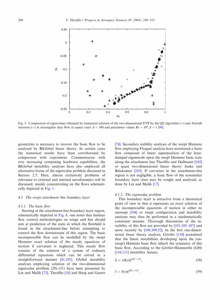
geometries is necessary to recover the basic flow to be

analysed by BiGlobal linear theory. In certain cases

the numerical results have been corroborated by

comparison with experiment. Commensurate with

ever increasing computing hardware capabilities, the

BiGlobal instability analyses have also employed all

alternative forms of the eigenvalue problem discussed in

Section 2.5. Here, almost exclusively problems of

relevance to external and internal aerodynamics will be

discussed, mainly concentrating on the flows schemati-

cally depicted in Fig. 1.

4.1. The swept attachment line boundary layer

4.1.1. The basic flow

Starting at the attachment-line boundary layer region,

schematically depicted in Fig. 6, one notes that laminar

flow control methodologies on wings and fins should

aim at prediction of the state at which the flowfield is

found in the attachment-line before attempting to

control the flow downstream of this region. The basic

incompressible flow can be modelled by the swept

Hiemenz exact solution of the steady equations of

motion if curvature is neglected. This steady flow

consists of the solution of a system of ordinary

differential equations which can be solved in a

straightforward manner [41,101]. Global instability

analyses employing solution of the two-dimensional

eigenvalue problem (28)–(31) have been presented by

Lin and Malik [73], Theofilis [18] and Heeg and Geurts

[74]. Secondary stability analyses of the swept Hiemenz

flow employing Floquet analysis have monitored a basic

flow composed of linear superposition of the least-

damped eigenmode upon the swept Hiemenz basic state

along the attachment line Theofilis and Dallmann [102]

or quasi two-dimensional linear theory Janke and

Balakumar [103]. If curvature in the attachment-line

region is not negligible, a basic flow of the nonsimilar

boundary layer class may be sought and analysed, as

done by Lin and Malik [17].

4.1.2. The eigenvalue problem

This boundary layer is attractive from a theoretical

point of view in that it represents an exact solution of

the incompressible equations of motion in either its

unswept [104] or swept configuration and instability

analyses may thus be performed in a mathematically

consistent manner. Thorough discussions of the in-

stability of this flow are provided by [101,105–107] and

more recently by [108,109,52]. In the first one-dimen-

sional linear theory analysis, G .ortler [110] postulated

that the linear instabilities developing upon the (un-

swept) Hiemenz basic flow inherit the symmetry of this

basic flow. According to the G .ortler-H.ammerlin (GH)

[110,111] instability Ansatz,

#u ¼ x *uðyÞeiðbz�otÞ; ð58Þ

#v ¼ *vðyÞeiðbz�otÞ: ð59Þ

0.05

0

−0.05

−0.1

−0.15

−0.2

−0.250 0.2 0.4 0.6 0.8 1

ωi

ωr

Fig. 5. Comparison of eigenvalues obtained by numerical solution of the two-dimensional EVP by the QZ algorithm ðþÞ and Arnoldi

iteration ð�Þ in rectangular duct flow at aspect ratio A ¼ 100 and parameter values Re ¼ 104; b ¼ 1 [99].


This idea was extended to the swept Hiemenz flow by

Hall et al. [101] who additionally assumed

#w ¼ *wðyÞeiðbz�otÞ ð60Þ

and solved an ordinary-differential-equation-based

linear eigenvalue problem of class (4) and (5) to recover

a critical Reynolds number RecritE581: This compares

very well with the results of both experiments performed

under linear conditions and several two- and three-

dimensional DNS studies; however, in the presence of

large-amplitude disturbances in the flow, subcritical

instability has been observed experimentally and in DNS

at a much lower ReE245 value [105,107].

Theofilis and Dallmann [102] employed the shape

assumption [57] for the secondary instability problem

and, staying within the bounds imposed by this

approach, showed that amplitudes of the primary

(decaying) GH mode of Oð1%Þ are sufficient to

excite secondary instability of both fundamental

and subharmonic type at Re > 250; as shown in Fig. 7.

On the other hand, motivated by the discrepancy in

linear critical Reynolds numbers Lin and Malik [73,17],

formulated and solved the two-dimensional eigenvalue

problem (28)–(31) in which the assumption on the

form of the disturbances in the streamwise direction x

has been relaxed. These investigators utilised the

symmetries of the basic flow in their analysis and

discovered new BiGlobal eigenmodes in the swept

Hiemenz case, the frequencies of which were documen-

ted as being very close to, while their growth rates

were found to be smaller than the respective

quantities of the GH eigenmode. In this respect, the

new modes cannot be held responsible within a linear

framework for subcritical instability in the swept

Hiemenz flow.

Theofilis [18] solved the partial-derivative eigenvalue

problem without utilising the symmetries of the basic

flow and documented the chordwise variation of the new

modes with respect to x: He went on to analyse the

spatial structure of the BiGlobal eigenmodes, the first

three of which are shown in Fig. 8. All BiGlobal flow

eigenmodes were classified into two families of sym-

metric and antisymmetric modes, discriminated by their

chordwise dependence. The analytical description of the

chordwise structure of the BiGlobal eigenmodes in terms

of polynomials in x was utilised to derive two ordinary-

differential-equation-based eigenvalue problems for the

symmetric

fP� 2M %u þ ibReOg *u2M�1 � %u0 *v2M�2 ¼ 0; ð61Þ

2ð2M � 1Þ½ %uDþ %u0 *u2M�1 þ fRþ ð2M � 1Þ %u00

þ ibReO½D2 � b2g*v2M�2 ¼ 0; ð62Þ

and the antisymmetric modes

fP� ð2M þ 1Þ %u þ ibReO *u2Mg *u2M � %u0 *v2M�1 ¼ 0; ð63Þ

4Mf %uDþ %u0g *u2M

þ fRþ 2M %u00 þ ibReO½D2 � b2g*v2M�1 ¼ 0: ð64Þ

External streamline surfaceCylinder surface

A

x

yx

zA

δ

V∞ W∞

WΘ

Q∞

y

Fig. 6. Schematic representation of the swept attachment-line boundary layer [105,52].


Here ð %u; %v; %wÞT denotes the swept Hiemenz basic flow,

M ¼ 1; 2;y denotes the discrete BiGlobal eigenmodes,

P ¼ D2 � %vD� b2 � ibRe %w;

R ¼D4 � %vD3 � ½2ðM � 1Þ %u þ %v0 þ ibRe %w þ 2b2D2

þ ½ %u0 þ b2%vDþ 2ðM � 1Þb2

%u þ b2%v0

þ b4 þ ib3Re %w þ ibRe %w00;

where D � d=dy: These systems allow the calculation of

the BiGlobal instability in the attachment-line region

and recover the eigenvalues of the temporal partial-

derivative eigenvalue problem results at a fraction of the

cost of solving (28)–(31). When written as a spatial

eigenvalue problem (61)–(64) yield results which are in

excellent agreement with those of the spatial DNS of

the attachment-line region [112] or the results of

the corresponding spatial partial-derivative eigenvalue

200.0 300.0 400.0 500.0 600.0 700.0

Re

−0.020

−0.015

−0.010

−0.005

0.000

0.005

0.010

σ r

Fundamental Secondary Growth β=0.3, α=0.2

LSTA=3.0%A=2.5%A=2.0%

0 200 400 600 800

Re

−0.06

−0.04

−0.02

0.00

σ

Subharmonic Secondary Growth β=0.3, α=0.2

LSTA=1.0%A=1.5%A=2.0%

Fig. 7. Secondary instability in the swept Hiemenz flow [102].


problem in this flow. The supergeometric decay of the

amplitude functions of all model eigenmodes as M-N;which accounts for finite results being delivered by the

three-dimensional extension of the GH model, is shown

in Fig. 9 at a particular set of values of the parameters

ðRe; bÞ: Fedorov (unpublished) has independently ar-

rived at the prediction of the instability results of [73]

through WKB analysis, which delivers results equivalent

to those obtained by solution of the one-dimensional

eigenvalue problem (61)–(64). A discussion of linear and

nonlinear instability in the three-dimensional swept

Hiemenz flow, including direct numerical simulations

initialised on the extended GH model eigenfunctions

may be found in [113]. Bertolotti [114] in his work on the

connection of attachment-line and crossflow instabilities

showed that the polynomial modes (61)–(64) are the

only families of linear disturbances relevant to instability

in the attachment-line region itself. The spatial BiGlobal

Fig. 8. Upper: The spatial structure of Rf #ug; If #ug;Rf #wg and If #wg; of the G .ortler-H.ammerlin (GH) mode, recovered as solution of

the two-dimensional eigenvalue problem (28)–(31). Middle: The spatial structure of components of the disturbance eigenvectors

pertinent to the global eigenmode A1. Lower: Same result for S2. Left two columns Rf #ug; right two columns Rf #wg:


eigenvalue problem has been solved by Heeg and Geurts

[74]. An interesting characteristic of this work from a

numerical point of view is its use of a high-order finite-

difference method in conjunction with Jacobi–Davidson

iteration; the latter permits solving eigenvalue problems

in which the eigenvalue appears either linearly or

nonlinearly at the same computing effort. Finally, Lin

and Malik [17] departed from the swept-Hiemenz flow

model and addressed the problem of instability in the

attachment-line region taking curvature into account

and solving the respective two-dimensional eigenvalue

problem. In line with analogous results using the one-

dimensional eigenvalue problem, curvature was found to

stabilise the flow.

In summary, BiGlobal instability analysis has deliv-

ered the full-spectrum of attachment-line eigenmodes

relevant to laminar-turbulent flow transition on account

of linear mechanisms. Owing to the simple nature of

the model basic flow it has been possible to model the

EVP results by solution of (61–64), thus aiding their

incorporation into engineering-prediction toolkits.

4.2. The crossflow region on a swept wing


Moving downstream of the attachment line on to the

portion of the flowfield where different degrees of

deflection of the flow in the freestream and in the

boundary layer result in the latter having an inflectional

profile, as schematically depicted in Fig. 10, a well-

understood primary inviscid linear instability mechan-

ism of the class (4) is encountered [115]. The amplifica-

tion of this primary instability leads to a saturated

nonlinear basic state, identified as the well-known

stationary or travelling crossflow vortices [116–118].

The basic flow on this portion of a swept wing is

obtained by superposition of results of one-dimensional

linear theory upon a boundary layer solution at

arbitrarily low levels [119,120] or by three-dimensional

DNS [92]. Other investigations solve the nonsimilar

boundary layer equations upon which the crossflow

vortex primary instability is superimposed as a result of

PSE computation [65,103]. Yet another possibility which

circumvents the need to solve the receptivity problem

associated with PSE is superposition of nonlinear

saturation states of the primary linearly unstable

solutions upon the latter [64]. However, Haynes and

Reed [121] have shown that the nonlinear PSE is the

methodology which delivers best agreement with experi-

ment as far as the saturated nonlinear crossflow-vortex

basic flow is concerned. All subsequent BiGlobal

instability analyses define a local coordinate system in

which the basic flow plane is locally normal to the axis of

the primary crossflow vortices. A visualisation of this

basic flow taken from the DLR experiment on crossflow

instability [118] is presented in Fig. 11.

0 1 2 3 4 5 6 7 8mode index

10−12

10−9

10−6

10−3

100

103

max

val

ueu

Sv

Sw

Su

Av

Aw

A

Fig. 9. Maximum values of amplitude functions of the extended GH model against mode index m at Re ¼ 800; b ¼ 0:255: uS ; vS ;wS ; pS

and uA; vA;wA; pA denote maximum values of *um; *vm; *wm; *pm of symmetric and antisymmetric modes, respectively.



The significance of crossflow vortices for swept wings

has prompted intense investigation into instability

mechanisms leading to breakdown of the nonlinear

saturated basic state to turbulent flow. The first

experimental evidence that a high-frequency secondary

instability is responsible for transition of the flow to

turbulence was provided in the swept cylinder experi-

ments of Poll [122], while Kohama et al. [123] were the

first to identify this mechanism on a swept wing.

Subsequent experimental [124–126] and a multitude of

numerical work has confirmed the existence of high-

frequency secondary instability, linear amplification of

which rapidly leads the flow to breakdown and

turbulence. Reibert et al. [124], Saric et al. [127] and

Saric and Reed [128] went on to exploit this phenom-

enon and offer efficient technological solutions for

laminar flow control in incompressible and supersonic

swept wing flows, respectively. High-frequency second-

ary instability has been addressed theoretically in a

number of papers, notably the DNS work of Hoegberg

and Henningson [129], Wintergerste and Kleiser [92] and

Wassermann and Kloker [130] and the analyses of

Fischer and Dallmann [119], Fischer et al. [120], Malik

et al. [65], Wintergerste and Kleiser [92], Janke and

Balakumar [103] and Koch et al. [64]. In all analyses the

two-dimensional eigenvalue problem has been solved by

taking the homogeneous flow direction to be aligned

with the axis of the crossflow vortices and resolving the

other two spatial directions using a Fourier Ansatz in

the direction parallel to the wall. The crossflow vortex

y

external streamline

chordwisecomponent

crossflowcomponent

x*

z*

Fig. 10. Schematic representation of a 3D boundary layer velocity profile [115].

Fig. 11. Flow visualisation of crossflow vortices, taken from

the experiment on the DLR swept wing [118].


axis is assumed to be straight, an assumption which can

be a posteriori justified by reference to the wavelengths

of the amplified high-frequency secondary disturbances.

A BiGlobal eigenvalue problem was formulated and

solved by Malik et al. [65], using a Krylov subspace

iteration method. The BiGlobal eigenmodes could be

classified in two families, while the predicted frequencies

of the two dominant modes were found to peak between

3.5 and 4:5 kHz: The spatial structure of these modes

was found to be consistent with available experimental

results. One such result, showing (in colour) the

structure of the high-frequency secondary instability

superimposed upon the crossflow vortices (dashed lines)

is shown in Fig. 12. However, Malik et al. [65] stressed

that in order for reliable transition-prediction criteria to

be provided, additional work is necessary on at least two

fronts, receptivity of the flow during the stages prior to

linear growth of the primary disturbances and the

correlation of transition onset location and onset of

the secondary instability. They pointed out that one

possible means to achieve this is through DNS which

takes into account onset of high-frequency secondary

instability, interaction of stationary and travelling

crossflow disturbances and nonlinearity. A step in

this direction was taken by Hoegberg and Henningson

[129] while work is in progress by Wintergerste and

Kleiser [92].

The latter authors studied the BiGlobal eigenvalue

problem by expanding the eigenfunctions into finite

Fourier–Chebyshev series, in view of the periodic

nature of the problem in the lateral spatial direction.

Use of the Arnoldi algorithm described in Section 3.2

was found to be essential for convergence of the results

in this work. During the early stages of the DNS

computation of the basic state, only low-frequency

Oð102Þ Hz secondary disturbances were found. As the

amplitude of the crossflow vortex rose beyond 10%

high-frequency secondary instability appeared, in line

with the results of Fischer et al. [120] who used the

simplifying assumption of a basic flow modified by

model linear primary eigenfunctions, as opposed to the

DNS-obtained basic state of [92]. As a matter of fact

two modes I and II were found by the latter authors in

the BiGlobal eigenspectrum, corresponding to frequen-

cies f ¼ 2134 and f ¼ 510 Hz; respectively. The corre-

sponding phase velocities were found to be cphE0:76

and 0.41, respectively. The spatial structure of the high-

frequency secondary instability eigenmodes corresponds

to elongated vortices located above the centre of the

crossflow vortex, at an angle of yE70� to it. As time

progresses the instability amplifies in an explosive

manner.

Janke and Balakumar [103] and Koch et al. [64] used

Floquet theory along the lines of (44) to solve the

BiGlobal eigenvalue problem. The first work focussed

on the existence of multiple roots of the eigenvalue

problem and the claim was put forward that this could

explain the origin of high-frequency instability and the

time-dependent occurrence of an exponential growth of

travelling disturbances observed in experiment. In the

second work, it was first stressed that the model basic

flow utilised had a universal character in terms of it

being independent of the receptivity problem. Earlier

findings on the large number of Fourier components in

Fig. 12. Saturated stationary primary crossflow vortex and superimposed secondary instability structure for the DLR-Experiment at

x=c ¼ 0:60 [103].


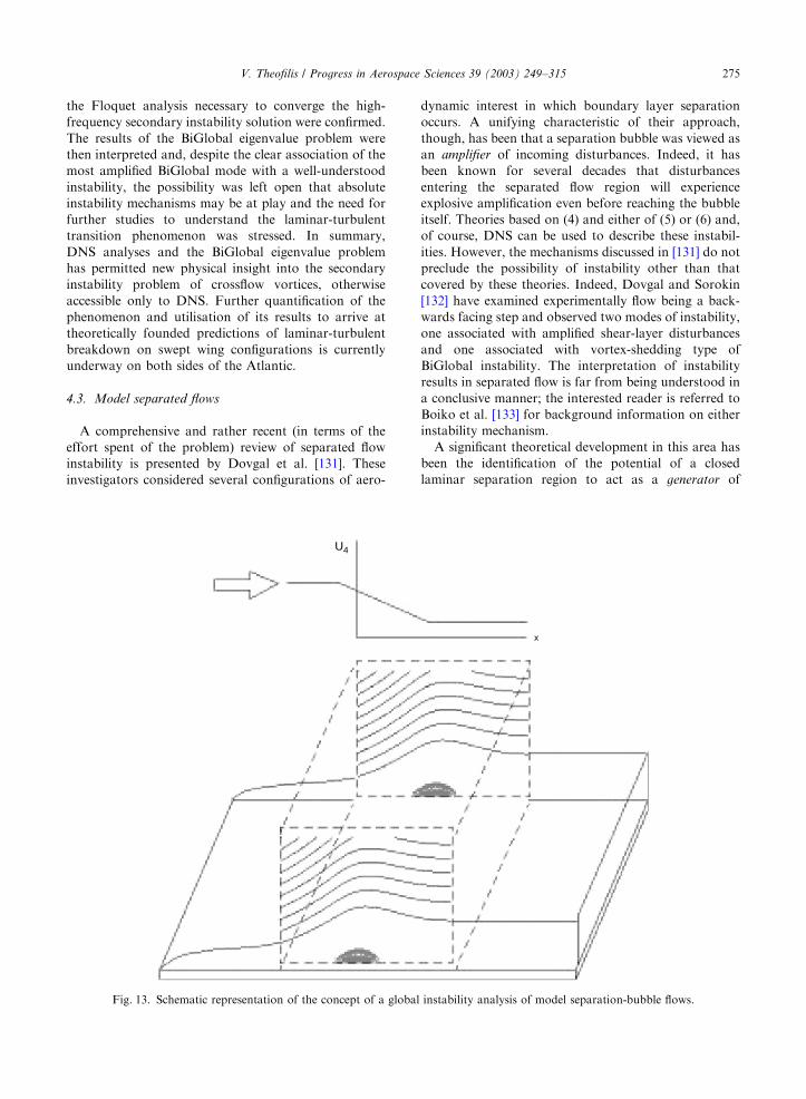
the Floquet analysis necessary to converge the high-

frequency secondary instability solution were confirmed.

The results of the BiGlobal eigenvalue problem were

then interpreted and, despite the clear association of the

most amplified BiGlobal mode with a well-understood

instability, the possibility was left open that absolute

instability mechanisms may be at play and the need for

further studies to understand the laminar-turbulent

transition phenomenon was stressed. In summary,

DNS analyses and the BiGlobal eigenvalue problem

has permitted new physical insight into the secondary

instability problem of crossflow vortices, otherwise

accessible only to DNS. Further quantification of the

phenomenon and utilisation of its results to arrive at

theoretically founded predictions of laminar-turbulent

breakdown on swept wing configurations is currently

underway on both sides of the Atlantic.

4.3. Model separated flows

A comprehensive and rather recent (in terms of the

effort spent of the problem) review of separated flow

instability is presented by Dovgal et al. [131]. These

investigators considered several configurations of aero-

dynamic interest in which boundary layer separation

occurs. A unifying characteristic of their approach,

though, has been that a separation bubble was viewed as

an amplifier of incoming disturbances. Indeed, it has

been known for several decades that disturbances

entering the separated flow region will experience

explosive amplification even before reaching the bubble

itself. Theories based on (4) and either of (5) or (6) and,

of course, DNS can be used to describe these instabil-

ities. However, the mechanisms discussed in [131] do not

preclude the possibility of instability other than that

covered by these theories. Indeed, Dovgal and Sorokin

[132] have examined experimentally flow being a back-

wards facing step and observed two modes of instability,

one associated with amplified shear-layer disturbances

and one associated with vortex-shedding type of

BiGlobal instability. The interpretation of instability

results in separated flow is far from being understood in

a conclusive manner; the interested reader is referred to

Boiko et al. [133] for background information on either

instability mechanism.

A significant theoretical development in this area has

been the identification of the potential of a closed

laminar separation region to act as a generator of

U4

x

Fig. 13. Schematic representation of the concept of a global instability analysis of model separation-bubble flows.


eigendisturbances and support BiGlobal instability in

the absence of incoming disturbances [134]. Further

detailed studies of the phenomenon using two different

model flows have been addressed independently by

Hammond and Redekopp [135] and Theofilis et al. [35];

the concept employed in either case is sketched in

Fig. 13.


In the work of Hammond and Redekopp [135] the

generic mechanism of BiGlobal instability4 was demon-

strated on the analytical model

%uðZÞ ¼ f 0ðZ; b0Þ � aZe�ðZ�Z0Þ=Z0 ; ð65Þ

where f is the solution to the Falkner–Skan equation5

subject to the boundary conditions

f ð0Þ ¼ f 0ð0Þ ¼ 0; f 0ðZ-NÞ ¼ 1; ð66Þ

where the parameters a; b0 and Z0 independently control

the strength of the backflow velocity and the depth of

the reversed-flow, which has been chosen to have

circular-arc dividing streamlines.

The mixed finite-difference/spectral algorithm de-

scribed in the appendix was used for the solution of

the boundary-layer equations in the BiGlobal instability

analysis of laminar separated flow model presented by

Theofilis et al. [35]. These authors solved the nonsimilar

boundary-layer equation (A.7) to obtain the inflow

boundary condition at x ¼ 0:05 for the subsequent two-

dimensional DNS of the separated flow region; the

algorithm also described in the appendix was used for

the DNS, in which parameters were chosen to match

those of Briley [137], while the inflow location was kept

constant at x0 ¼ 0:202 to ensure a well-defined recircu-

lation region [138]. The vorticity and two integral

quantities of the closed separation bubble flowfield thus

obtained are presented in Fig. 14. The total divergence

of these results, defined as

d ¼XNx

ix¼0

XNy

iy¼0

Dx %uðix; iyÞ þDy %vðix; iyÞ; ð67Þ

is d ¼ 6:6 � 10�8; implying satisfaction of the continuity

equation to within 5 � 10�11 at this resolution.

4.3.2. The eigenvalue problems

Hammond and Redekopp [135] performed a global

(in the classic sense) instability analysis within the

framework of WKB theory, in which the basic state

and its instabilities are assumed to develop on different

spatial scales. This assumption facilitates the numerical

work in that instead of the two-dimensional eigenvalue

problem (34)–(37) a sequence of Orr–Sommerfeld

equations may be solved at successive downstream

locations within the bubble. However, instead of

following the classic temporal or spatial OSE models,

in the two-dimensional limit of which the parameters

ða;OÞ in (5) are real/complex and complex/real respec-

tively, the OSE problem for this type of global instability

analysis is solved taking both a and O to be complex

quantities. The dispersion relation

Dða;O;ReÞ ¼ 0 ð68Þ

was used to compute a growth rate for BiGlobal

instability through the requirement that the group

velocity

@O=@aja0¼ 0 ð69Þ

at a particular a0: Note, this dispersion relation contains

parameters defined in (65). The instability analysis

showed that model separated flow can become BiGlob-

ally unstable when the peak reversed flow in the bubble

reaches about 30% of the freestream value. These

authors went on to associate their result with the

experimental evidence on pitching aerofoils and dy-

namic stall that time-dependent large-scale dynamics

lead to collapse of the separated flow region when the

latter approaches about 40% of the free-stream value.

The question of the shape of the BiGlobal eigenmode

and its possible implication for flow control will be

revisited in Section 4.12.

Theofilis et al. [35] have employed one-dimensional

(OSE), quasi-two-dimensional (PSE) and two-dimen-

sional (BiGlobal) analyses to study numerically the

instability of incompressible steady laminar boundary-

layer flow which encompasses a recirculation bubble.

Both stationary and pairs of travelling linear instabilities

were discovered, which are distinct from known solu-

tions of the linear OSE or linear PSE instability theories,

and can both become unstable at sufficiently high

backflow strength, at the present parameters of the

Oð10%Þ: It should be mentioned that at these parameters

Tollmien–Schlichting instability has a wavelength which

is an order of magnitude smaller than a typical scale of

the BiGlobal eigenmode amplitude functions and its

growth rates are approximately two orders of magnitude

smaller than those of TS instability. A conjecture on the

consequence of this disparity in amplification rates of

the two instability mechanisms Theofilis [139] has

suggested that, although the classic TS mechanism

may act as a catalyst for laminar breakdown, attention

must be paid to the control of BiGlobal instability of the

flow as a precursor to vortex-shedding and a mechanism

relevant to turbulent flow control, in a manner that will

be discussed in what follows.

4This basic state is one in which the concepts of global

instability, as used by earlier theoretical analyses of weakly

nonparallel flows and in the present sense of inhomogeneous

two-dimensional basic flows, coincide.5A special case of the nonsimilar boundary layer equations

(A.7) and prime denotes differentiation w.r.t. Z: [136].


The spatial structure of the most unstable BiGlobal

eigenmode, recovered by solution of the real eigenvalue

problem (34)–(37) at ReE1:7 � 104; is shown in Fig. 15.

The innocuous nature of the primary separation line

alongside the three-dimensionalisation of the primary

reattachment region is shown in Fig. 16, where an

isosurface of the disturbance vorticity is shown at an

arbitrary level. The primary separation bubble is

contained within the dashed lines and paths of particles

released in the flow provide a qualitative demonstration

of the effect of the BiGlobal eigenmode on the closed

streamlines of the basic flow. The recovery of unstable

eigenvalues in the problem at hand must be seen in the

perspective of the artificial (from a physical point of

view) homogeneous Dirichlet inflow boundary condi-

tions. In practice, Tollmien–Schlichting instability in the

flow under consideration is orders of magnitude

stronger than the BiGlobal mechanism, at least in the

bracket of parameters monitored by Theofilis et al. [35].

Recent numerical efforts [140] have independently

confirmed the existence of BiGlobal instability at the

parameters of [35], although later efforts (Hetsch,

personal communication) have attributed the results of

[140] to insufficient numerical resolution. This further

0.025

0.02

0.03

0.015

0.01

0.005

0

−0.5

−1

−1.5

−2

−2.5

−3

−3.5

−4

−4.5

−5

0.50.4 0.450.350.30.250.20.150.10.05

y

× 104

Xo : present solution; -- : Blasius theory o : present solution; -- : Blasius theory

1.6

1.4

1.2

1

0.8

0.6

0.4

0.20 0.1 0.2 0.3 0.4 0.50.450.350.250.150.05

δ* (

x)

1.2

1

0.8

0.6

0.4

0.2

0

−0.2

τ (x

)

x0 0.1 0.2 0.3 0.4 0.50.450.350.250.150.05

x

Basic Flow Vorticity

Fig. 14. Basic flow vorticity z ¼ @%v=@x � @ %u=@y (upper) and integral quantities of the [137] separation bubble.


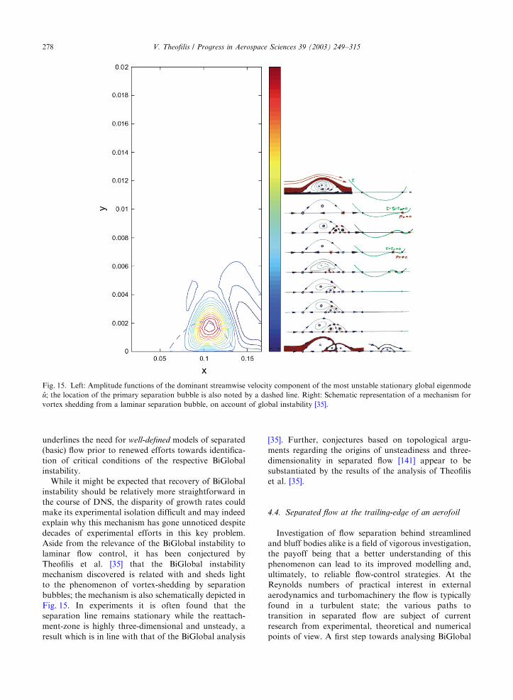
underlines the need for well-defined models of separated

(basic) flow prior to renewed efforts towards identifica-

tion of critical conditions of the respective BiGlobal

instability.

While it might be expected that recovery of BiGlobal

instability should be relatively more straightforward in

the course of DNS, the disparity of growth rates could

make its experimental isolation difficult and may indeed

explain why this mechanism has gone unnoticed despite

decades of experimental efforts in this key problem.

Aside from the relevance of the BiGlobal instability to

laminar flow control, it has been conjectured by

Theofilis et al. [35] that the BiGlobal instability

mechanism discovered is related with and sheds light

to the phenomenon of vortex-shedding by separation

bubbles; the mechanism is also schematically depicted in

Fig. 15. In experiments it is often found that the

separation line remains stationary while the reattach-

ment-zone is highly three-dimensional and unsteady, a

result which is in line with that of the BiGlobal analysis

[35]. Further, conjectures based on topological argu-

ments regarding the origins of unsteadiness and three-

dimensionality in separated flow [141] appear to be

substantiated by the results of the analysis of Theofilis

et al. [35].

4.4. Separated flow at the trailing-edge of an aerofoil

Investigation of flow separation behind streamlined

and bluff bodies alike is a field of vigorous investigation,

the payoff being that a better understanding of this

phenomenon can lead to its improved modelling and,

ultimately, to reliable flow-control strategies. At the

Reynolds numbers of practical interest in external

aerodynamics and turbomachinery the flow is typically

found in a turbulent state; the various paths to

transition in separated flow are subject of current

research from experimental, theoretical and numerical

points of view. A first step towards analysing BiGlobal

Fig. 15. Left: Amplitude functions of the dominant streamwise velocity component of the most unstable stationary global eigenmode

#u; the location of the primary separation bubble is also noted by a dashed line. Right: Schematic representation of a mechanism for

vortex shedding from a laminar separation bubble, on account of global instability [35].


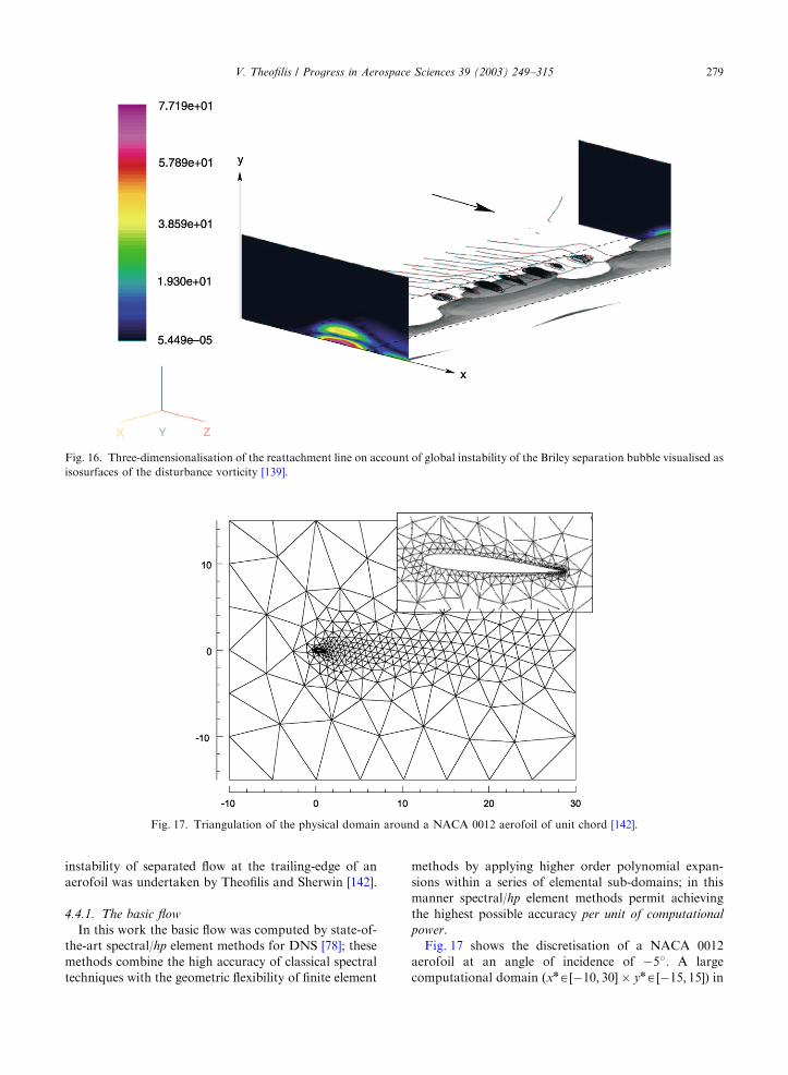
instability of separated flow at the trailing-edge of an

aerofoil was undertaken by Theofilis and Sherwin [142].


In this work the basic flow was computed by state-of-

the-art spectral/hp element methods for DNS [78]; these

methods combine the high accuracy of classical spectral

techniques with the geometric flexibility of finite element

methods by applying higher order polynomial expan-

sions within a series of elemental sub-domains; in this

manner spectral/hp element methods permit achieving

the highest possible accuracy per unit of computational

power.

Fig. 17 shows the discretisation of a NACA 0012

aerofoil at an angle of incidence of �5�: A large

computational domain ðxnA½�10; 30 � ynA½�15; 15Þ in

Fig. 17. Triangulation of the physical domain around a NACA 0012 aerofoil of unit chord [142].

XX Y Z

Fig. 16. Three-dimensionalisation of the reattachment line on account of global instability of the Briley separation bubble visualised as

isosurfaces of the disturbance vorticity [139].


chord length c units was chosen to remove any influence

of the artificial computational boundaries. A key point

regarding the accuracy of this basic flow is that the

geometry of the aerofoil was consistently described by

isoparametric elements, e.g. the surface was represented

by a similar order polynomial order within each element

as that in the solver itself. The calculations were

performed at a chord Reynolds number Rec ¼ UNc=n ¼103 where UN is the magnitude of the free stream

velocity, c is the chord length and n is the kinematic

viscosity of the fluid. The aerofoil was assumed to have a

finite trailing-edge thickness of 0:003c and so the local

Reynolds number based on the trailing-edge was Retr ¼3; which is well below typical bluff body vortex shedding

values of approximately 50. At this Reynolds number

one of the most interesting features of the flow is

trailing-edge separation, visualised in Fig. 18. The high-

lighted part of the flow was extracted from the

simulation data, rotated by an angle fE� 12� and

interpolated on a rectangular cartesian grid approximat-

ing a body-fitted coordinate system and extending

between xA½0:714; 0:992 � yA½0:199; 0:2589 to form

the basic flow of the BiGlobal instability analysis.


In a manner analogous to the model separated flow

problems of Section 4.3 the two-dimensionality of the

basic state suggests ability to solve the real eigenvalue

problem (34)–(37). For reasons of numerical feasibility

but also in order to monitor instability mechanisms

potentially generated on account of the trailing-edge

separated region in isolation from other instabilities

present in this flow Theofilis and Sherwin [142] solved

the two-dimensional eigenvalue problem using a rectan-

gular standard Chebyshev grid mapped onto the high-

lighted part of the flow shown in Fig. 18 through an

algebraic transformation. In order to prevent distur-

bances potentially existing upstream of the upstream

boundary of the monitored domain from entering the

trailing-edge region, homogeneous Dirichlet boundary

conditions were imposed on all disturbance amplitude

functions at this boundary. No slip conditions were

imposed on the disturbance velocity components at the

wall, where the compatibility conditions (50) and (51)

were imposed on pressure. At the farfield boundary,

homogeneous Dirichlet conditions have been imposed

on all disturbance amplitude functions. Finally, at the

outflow boundary a linear extrapolation procedure has

been used.

The wavenumber parameter space was examined,

taking the periodic spanwise extent of the domain

Lz=LxA½1=8; 32; where LxE0:278 is the streamwise

extent of the separated region monitored, which results

in bA½0:7; 180: Only damped eigenmodes have been

found in this wavenumber range at this modest

Reynolds number. The spatial structure of the spanwise

disturbance velocity component #w of the least damped

eigenmode is shown in Fig. 19 at Lz=LxE1; as a matter

of fact the qualitative structure of the least damped

eigenmode is practically independent of b such that this

Fig. 18. Steady laminar separated in the trailing-edge of a NACA 0012 aerofoil at chord Re ¼ 103 and angle of incidence �5� [142].


result can be considered representative of those obtained

at different wavenumber values. The #w component of

the BiGlobal eigenvector is interesting in that the actual

three-dimensionalisation of the flow is determined by its

structure when the eigenmode becomes unstable. The

structure of *w is reminiscent of that found in the laminar

separation bubble problem of Howarth/Briley, as

discussed in the previous section; the basic flow

recirculation zone will be split into two regions of fluid

travelling in the opposite directions along the

z-coordinate. The critical Reynolds number at which

this will occur is the subject of current investigations.

The key discovery of global instabilities in separated

flow alongside the prevalence of the phenomenon of

flow separation in aeronautics warrant, in the author’s

view, renewed efforts in order to arrive at a more

complete understanding of all instability mechanisms

related to flow separation.

4.5. Flows over steps and open cavities

4.5.1. The basic flows

Open systems of practical importance in the context

of aeronautics are the backward and forward facing

steps, that over rectangular two-dimensional protrusions

from a flat plate as well as open cavity configurations.

All can be used as elementary models of parts of a high-

lift configuration. Different methodologies have been

followed for the recovery of the basic flow in these cases

by the investigators who solved the respective BiGlobal

instability problems. Barkley et al. [143] have used a

spectral element discretisation of the backward facing

step and Newton iteration for the two-dimensional basic

state, which was obtained as the zeroth Fourier mode of

the same three-dimensional spectral element numerical

scheme also employed for the subsequent instability

analysis. St .uer [82] and St .uer et al. [144] calculated the

basic flow in the forward-facing step employing a

second-order finite-volume method incorporating a

projection step for the decoupled calculation of velocity

and pressure fields. McEligot and co-workers [145] have

produced benchmark experimental results for (three-

dimensional) flow over a two-dimensional rectangular

protrusion, covering Reynolds number ranges low

enough so that well upstream and downstream of the

protrusion essentially Blasius flow is established, up to

such Reynolds numbers that flow is turbulent immedi-

ately downstream of the protrusion; no analysis of these

experiments has been undertaken to-date.

The basic flow in open cavities of different aspect

ratios was solved using 6th-order compact finite-

differences [146] and a spectral multidomain algorithm

[40] to recover solutions in compressible and incom-

pressible open cavities, respectively. Interestingly, in

both the backward facing step and the open cavity the

shear layer emanating from the upstream corner

becomes unsteady in two and unstable in three spatial

dimensions in the context of the one-dimensional linear

local theory discussed in Section 2. This has diverted

attention of past investigations from the possibility of

the entire two-dimensional separated flow in either the

steps or the open cavity flows become unstable to three-

dimensional spanwise periodic BiGlobal linear instabil-

ities. The related conjecture is that a BiGlobal instability

may act in these flows alongside the local instability, the

origin of which is in the shear layer, in a manner

analogous to that of separated flow on flat surfaces

[135,35], and be responsible for the appearance of the

currently little-understood so-called wake-mode in-

stability [146]. Furthermore, if stores exist inside an

open cavity the steady basic flow pattern is strongly

affected; a demonstration can be found in Fig. 22. It

may be inferred from this result that instability of the

shear layer at the upstream wall may only partly be held

responsible for the complex physical instability mechan-

isms encountered in experiments and three-dimensional

simulations [9].

4.5.2. Eigenvalue problems and DNS-based BiGlobal

instability analyses

Barkley et al. [143] have considered the stability of

steady flow in a backward-facing step of inlet-to-outlet

Fig. 19. Amplitude functions of the spanwise disturbance

velocity component *w developing upon the basic flow of

Fig. 18; upper Rf *wg; lower If *wg [142].


height 1:2 in the range of Reynolds numbers (built

with the centreline value of the parabolic velocity

profile upstream of the step and the step height)

ReA½450; 1050: They used DNS and a Krylov subspace

iteration method for the determination of the most

unstable eigenvalues, in both cases discretising space by

a spectral-element method. One advantage of the latter

is the ability to retain the same grid for both the basic

flow and the eigenvalue problem but use the order of the

expansion within elements to ensure convergence of the

numerical results at modest resolution. These authors

determined the critical conditions for the specific step

geometry to be Recrit ¼ 750; b ¼ 0:9; i.e. the flow

becomes three-dimensional to a BiGlobal eigenmode

having a spanwise periodicity of approximately seven

step heights. This critical Reynolds number value is

substantially higher than those reported in experiments

and DNS; however the intricate interplay of convective

instability of the shear layer emanating at the lips of the

step and BiGlobal instability of the entire recirculation

bubble behind the step are far from being understood in

a satisfactory manner for comparisons of the Reynolds

number(s) to be made. The leading eigenmode of the

BiGlobal instability has a spatial structure concentrated

in the region immediately downstream of the step corner

and, significantly, within the primary recirculation

region, manifesting itself as a three-dimensionalisation

of the basic-flow reattachment line. The latter aspect

makes the BiGlobal instability mechanism in this flow

qualitatively analogous to that of the pressure-gradient

induced separation on a flat plate [35]. Barkley et al.

[143] also addressed the issue of instability of the flow to

two-dimensional BiGlobal eigenmodes. Based on extra-

polation of damping-rate results these authors asserted

that unsteadiness of the two-dimensional flow is

expected beyond Re ¼ 1350:St .uer [82] and St .uer et al. [144] employed the same

finite-volume algorithm used for the solution of the

basic flow problem to calculate the BiGlobal instability

of the forward-facing step. Their work covered a range

of step-height based Reynolds numbers ReA½10; 200:On grounds of computing expediency these investigators

have used the same grid for the calculation of the basic

flow and the eigenvalue problem so their results cannot

be considered definitive until confirmed by higher-

resolution calculations or by a different high-order

numerical method. In the parameter range examined,

pertinent to a step-to-channel height ratio 0.5, they

reported stability of the flow at Re ¼ 50; instability of a

stationary eigenmode at Re ¼ 100 and instability of

several travelling modes at Re ¼ 150 and 200; they

concluded that the 1:2 forward-facing step flow loses

stability to three-dimensional travelling disturbances at

ReE75:Theofilis [40] obtained incompressible flows over open

cavities of different aspect ratios at Reynolds numbers

which were chosen to be low enough such that no

unsteadiness of the shear-layer was encountered. Char-

acteristic results are shown in Fig. 20. Several models of

the steady flowfield were analysed and the potential for

BiGlobal instability of the flow, in the absence of shear-

layer instability, was shown. At the other end of flow

speeds, namely hypersonic flow, recent experimental and

numerical investigations qualitatively relate flow over a

so-called ‘open’ configuration of the open cavity with

incompressible lid-driven rectangular cavity flow [147].

In the former case the shear layer formed at the

upstream lip of the open cavity spans the entire width

of the cavity and acts as a lid which isolates slow flow

inside from that outside the open cavity. Inside the

cavity the steady basic flow pattern resembles quite

closely that of incompressible lid-driven cavity flow at

moderate Reynolds number and comparable aspect

ratios; the instability of the lid-driven cavity flow will

be discussed in the next section.

Only DNS-based analyses of compressible open cavity

flow are available [146,9]. Given the predominant role

that the unsteady shear layer plays in this flow much

effort is devoted towards analysing this essentially one-

dimensional instability mechanism which can be

formulated using (4) and either of (5) or (6), with

appropriate acoustic forcing generated by interaction of

the shear-layer with the downstream edge. However, the

existence of a wake-mode instability [148] has raised

intriguing questions, since its appearance cannot be

explained using one-dimensional theory. Clearly a full

understanding of all instability mechanisms, including

those relevant to more complex cavities, is warranted.

Some progress towards understanding was made by

Colonius et al. [146], who found that the frequencies of

oscillation of the wake-mode instability were nearly

independent of the Mach number, over the range

0:2oMo0:8; indicating that acoustic feedback did not

play a role in the instability. They conjectured that

wake-mode BiGlobal instability was related to a

stronger recirculating flow within the cavity than that

which exists in the shear-layer-mode.

Theofilis et al. [149] have analysed the steady two-

dimensional basic state obtained in a length-to-depth

ratio L=D ¼ 2 cavity flow at incoming boundary layer

displacement thickness Rey ¼ 51 and Mach number

M ¼ 0:2; shown in Fig. 20. The #u disturbance velocity

component of the least damped two-dimensional ðb ¼ 0Þeigenmode of this flow is shown in Fig. 21; the most

interesting characteristic of this BiGlobal eigenmode is

its spatial shape, composed of a large-scale structure

inside the cavity, reminiscent of the most unstable

BiGlobal eigenmode in the lid-driven cavity (see below)

and possibly related with the wake-mode, and a well-

defined Tollmien–Schlichting instability developing on

the downstream wall of the cavity. Moreover, this least-

stable eigenmode shows no sign of a shear-layer related


eigenfunction. This counter-intuitive result is rather

intriguing and points to the need for further work to

quantify the relationship and relative significance of this

BiGlobal instability mechanism with that in the shear-

layer. This is even more compelling if an understanding

of instability in 3D and/or full-store configurations is

Fig. 20. Qualitative modification of the incompressible steady low-Re flow inside an open cavity on account of the presence of a model

store.


to be achieved. This understanding is in the author’s

view a prerequisite for physically based efficient model-

ling and control in this flow.

4.6. Flow in lid-driven cavities

Three interesting classes of duct flows are schemati-

cally presented in Fig. 23; they correspond to pressure-

driven flow in rectangular ducts having stationary walls

(left) and duct flows driven by a lid which makes an

angle f with the axis Ox: The case f ¼ 0 is the classic

(rectangular) lid-driven cavity while f ¼ p=2 corre-

sponds to the two-dimensional analogon of Couette

flow. All three classes have been studied in detail by

Theofilis et al. [37].

4.6.1. The basic flows

The instability analysis in a lid-driven cavity flow,

schematically depicted in Fig. 24, has clearly demon-

strated the challenges presented by a BiGlobal linear

analysis on account of poor resolution of the basic flow.

The square lid-driven cavity has attracted considerable

interest with respect to its BiGlobal linear instability by

Ramanan and Homsy [81], St .uer [82], Ding and

Kawahara [150,84] and Theofilis [40]. Ramanan and

Homsy [81] used high-order accurate finite-differences,

while Ding and Kawahara [150,84] used a finite-element

methodology and St .uer [82] addressed this flow as part

of the validations of a finite-volume algorithm. Theofilis

[40] solved the basic flow problem using the spectral

collocation algorithm of Appendix A. The accuracy of

the obtained steady-state solutions has been assessed by

comparison with the established works of Ghia et al.

[151] and Schreiber and Keller [152] and converged basic

states calculated at several Reynolds numbers and

presented at Re ¼ 1000 and 4000 in Table 4 demonstrate

a satisfactory agreement with both benchmark works at

the lower Re-value and especially with the Richardson

extrapolated results of Schreiber and Keller [152] at the

higher Reynolds number value monitored.

A different cavity flow configuration has been

addressed by Kuhlmann and co-workers [83,153]. These

authors considered basic flows set up by motion of two

facing walls in opposite directions, which they mon-

itored experimentally and analysed numerically. The

4

3

2

1

0

−10 2 4

Y

X

Fig. 21. Streamwise basic flow velocity component %u of

compressible flow in an open cavity [146,9].

6

5

4

3

2

1

0

−10 5

X

Y

Fig. 22. Streamwise disturbance velocity component #u in compressible flow over an open cavity at length-to-depth ratio 2, Rey ¼ 51

and M ¼ 0:2 [149].


basic flow was described by two Reynolds numbers built

with the aid of the speeds of the moving lids. Kuhlmann

et al. [83] used a two-dimensional finite-difference/

spectral-collocation DNS algorithm to calculate the

basic states. To overcome the singularity in the

boundary conditions at the junctions of stationary and

moving cavity walls, these authors regularised the lid-

velocity analytically and asserted that their chosen

procedure affected the instability results maximally by

a few percent. Furthermore, they justified the use of a

two-dimensional solution procedure for the recovery of

the basic state by comparison with experimental results

in the neighbourhood of the plane of symmetry z ¼ 0 of

the configuration monitored. Based on their BiGlobal

instability analysis results at the appropriate limit

Kuhlmann et al. [83] questioned the accuracy of the

BiGlobal instability analysis results of Ramanan and

Homsy [81], thus raising renewed interest in the

BiGlobal instability analysis of the classic (one-sided)

lid-driven cavity flow.


This has been addressed by numerical solution of the

real eigenvalue problem (34)–(37) in [150,84,82,40] or of

x

z

y

Fig. 24. Global instability analysis concept in a driven-cavity.

x

y

z

φ

Fig. 23. Schematic representation of pressure-gradient driven flow in a duct with four stationary walls (left) and of flow driven by the

motion of one wall which slides with constant velocity making an angle j with the axis Ox (right).


a reduced form of this system in which a lower number

of equations must be solved6 in [81]. Furthermore,

different numerical means, consistent with those used by

the different investigators for the calculation of the basic

flow, have been employed for the spatial discretisation

of the eigenvalue problem. While the experimentally

established stability of the two-dimensional basic state

at low Reynolds numbers, i.e. two-dimensionality of the

flow at these conditions [154], is reproduced in all

available analyses, only those of Ding and Kawahara

[84] and Theofilis [40] have produced consistent results

at high Reynolds numbers as far as the third most

unstable BiGlobal eigenmode is concerned. In the last

work two additional eigenmodes were discovered, one

stationary and one travelling. The critical parameters of

the most unstable stationary mode S1 are Recrit;S1 ¼ 783

at b ¼ 15:4; those of the first travelling eigenmode T1

are ðRecrit;T1 ¼ 845; b ¼ 15:8Þ while the respective para-

meters of the previously known mode T2 [84] are

ðRecrit;T2 ¼ 922; b ¼ 7:4Þ: The frequency of the most

unstable travelling mode T1 shows very good agreement

with experimentally obtained frequency results of

Benson and Aidun [155], as shown in Fig. 25. The

spatial structure of two components of the (stable) two-

dimensional ðb ¼ 0Þ eigenvector of a square cavity at

Re ¼ 1000 is shown in Fig. 26 with the values of the

marked levels cited in Table 5; both the spanwise

disturbance velocity component #w and the disturbance

pressure #p are seen to acquire the vortical structure of

the underlying two-dimensional basic flow [154]. The

spatial structure of the most unstable three-dimensional

eigenmode is shown in Fig. 27 as isosurfaces of the

disturbance vorticity. It is interesting to note that such a

structure might be confused with nonlinear flow

behaviour in flow visualisations of experimental or

DNS results, although it is the result of a BiGlobal

linear mechanism.

The two-sided lid-driven cavity flow [83] is in certain

ways analogous to the one-sided lid-driven cavity, but

important differences also exist. The second Reynolds

number introduces an additional control parameter in

the problem. Keeping the two Reynolds numbers at the

same value (‘symmetric driving’) Kuhlmann et al. [83]

discussed the hysteresis loop encountered in the range

ReA½234; 427 from the point of view of its instability to

two-dimensional BiGlobal infinitesimal disturbances

and showed that the flow is unstable within this bracket

of Reynolds numbers and linearly stable at Reo234;where it is found in a two-vortex state, as well as at

Re > 427; where a cats eye structure is the prevalent flow

configuration. However, the latter flow is unstable to

three-dimensional perturbations, the critical conditions

of which are a function of the cavity aspect ratio A: The

minimum critical Reynolds number was found to be

ReE190 at b ¼ 2:4 and A ¼ 1:45: A different type of

instability was also documented in the experiments,

namely the appearance of multiple cells as the Reynolds

number increases, which is another discriminating

characteristic between the one- and two-sided lid-driven

cavity flows. Finally, based on their experimental and

numerical results, Kuhlmann et al. [83] proposed that in

the two-vortex state the diameter D of the main inviscid

vortex core scales linearly with the cavity aspect ratio,

as opposed to DBRe1=2 that Pan and Acrivos [156]

Table 4

Comparison of the interpolated values of our solutions on the maxima presented by [151] (GGS) and [152] (SK)

Re ¼ 1000

Primary UL LL LR

c z c z 104c z 103c z

GGS �0:117929 2:04968 2:31129 �0:36175 1:75102 �1:1547

Present �0:118902 2:06839 2:37806 �0:36575 1:77911 �1:1486

SK �0:11894n 2:0677n 2:1700 �0:302000 1:700 �0:9990

Present �0:118905 2:068234 2:3151 �0:312162 1:763 �1:0481

Re ¼ 4000

Primary UL LL LR

c z c z 103c z 103c z

SK �0:12202n 1:9498n 1:1200 �1:0670 2:8000 �2:14500

Present �0:122026 1:94960 1:2411 �1:1427 2:9228 �2:31944

An asterisk denotes Richardson-extrapolated data in the latter work.

6Although higher-order derivatives appear, which are more

challenging to represent numerically when using a moderate

number of discretisation points.


β

Re700 750 800 850 900 950 1000 1050 1100 1150 12000

5

10

15

20

25

30

ωr

Re700 750 800 850 900 950 1000 1050 1100 1150 12000

0.05

0.1

0.15

0.2

0.25

Fig. 25. Upper: theoretical neutral loops in the square lid-driven cavity. Lower: dependence of the frequency of the three most unstable

global eigenmodes on Reynolds number and their comparison with experimental results of [155] denoted by star symbols; note, the

most unstable mode is stationary, Or � 0 [40].


0 0.1 0.2 0.3 0.4 0.5 0.6 0.7 0.8 0.9 10

0.1

0.2

0.3

0.4

0.5

0.6

0.7

0.8

0.9

1

x

y abcdefgh

0 0.1 0.2 0.3 0.4 0.5 0.6 0.7 0.8 0.9 10

0.1

0.2

0.3

0.4

0.5

0.6

0.7

0.8

0.9

1

x

y

a

ab

c

c

c

d

ef

gh

i

j

d

Fig. 26. Isolines of disturbance velocity component #w and disturbance pressure #p of the two-dimensional (b ¼ 0Þ global mode at

Re ¼ 103 in a square lid-driven cavity [40].


predicted in the limit A-N of an one-sided lid-driven

cavity.

4.7. Flows in ducts and corners

4.7.1. Basic flows

Besides the handful of basic flows directly relevant to

aeronautics which have been addressed by BiGlobal

instability analysis to-date, several simple model flows

which generalise analytically known one-dimensional

steady profiles have been monitored with respect to their

BiGlobal instability. Tatsumi and Yoshimura [14]

studied the instability of flow in a rectangular duct,

while Kerswell and Davey [157] addressed that of flow in

a duct of elliptic cross section. The limit of large aspect

ratio in the first flow and that of large eccentricity in the

second approximate plane Poiseuille flow, while the case

of unit eccentricity in the elliptic duct corresponds to one

of the best known failures in the predictions of classic

one-dimensional linear instability theory, namely

Hagen–Poiseuille flow. In both the case of basic flow

in a rectangular duct and that in the elliptic pipe analytic

solutions are known for the single nonzero velocity

component %w set up when flow is driven by a constant

pressure gradient along the homogeneous spatial direc-

tion z: In a rectangular duct defined in the domain S ¼fxA½�A;Ag � fyA½�1; 1g; where A is the aspect ratio

(all lengthscales being nondimensionalised with respect

to the duct semi-depth), the steady laminar flow is

independent of z and possesses a velocity vector

ð0; 0; %wÞT: Taking the constant pressure gradient value

d %p=dz ¼ �2 and scaling the result with the value of %w at

the midpoint of the duct, the Poisson problem may be

solved in series form [136]

%wðx; yÞ ¼ 1 � y2 � 42

p

� �3XNn¼0

ð�1Þn

ð2n þ 1Þ3

�cosh½ð2n þ 1Þpx=2cos ½ð2n þ 1Þpy=2

cosh½ð2n þ 1ÞpA=2: ð70Þ

The plane Poiseuille basic flow result is retrieved from

this expression in the limit A-N: In the analysis of

Theofilis et al. [37] the basic flow problem was solved

numerically; an 8 � 8 Legendre collocation grid suffices

to obtain a solution of the two-dimensional Poisson

problem the relative deviation of which from the

analytic solution is less than 10�8 while analyses were

performed using upwards of 482 Legendre collocation

y

x

Fig. 27. Isosurface of disturbance vorticity magnitude in a square lid-driven cavity [40].

Table 5

Isoline levels of the results of Fig. 25

#w Symbol a b c d e f g h

Level 0.90 0.70 0.50 0.30 0.10 0.00 �0:10 �0:20

#p Symbol a b c d e f g h i j

Level 0.90 0.80 0.70 0.60 0.45 0.30 0.15 0.00 �0:15 �0:20


points. A different extension of the classic plane

Poiseuille flow has been addressed by Ehrenstein [16]

who solved the BiGlobal eigenvalue problem in a

channel one wall of which was covered by riblets. Here

the basic flow was obtained by solution of the

appropriate two-dimensional Poisson problem (15),

after an analytic description of the riblet geometry was

provided.

Yet another two-dimensional duct flow which has a

classic analytically known one-dimensional counterpart

has been investigated recently with respect to its

BiGlobal instability, namely wall-bounded Couette flow

between parallel plates defined by xA½�A;A and

yA½�1; 1 set up by keeping three walls at rest and

permitting the fourth to move at a constant speed along

the homogeneous direction, in the absence of a pressure

gradient. Normalising the moving-wall speed to %wðy ¼1Þ ¼ 1 it is straightforward to solve the homogeneous

two-dimensional Poisson equation (15) subject to

inhomogeneous boundary conditions and derive an

analytic solution for the basic flow %w [37]

%wðx; yÞ ¼XNn¼0

4ð�1Þn

ð2n þ 1Þpsinhð2n þ 1Þpðy þ AÞ=2

sinhð2n þ 1ÞpA

� cosð2n þ 1Þpx=2; ð71Þ

an expression which merges into the linear profile in the

limit A-N: Finally, flow in a sudden-expansion pipe

has recently received attention with respect to its

BiGlobal instability by Hawa and Rusak [39]. These

investigators obtained the basic state in a slightly

asymmetric channel numerically by solving (16) and

(17) using finite-difference techniques before employing

asymptotic expansions in the framework of a bifurcation

analysis to address the instability problem.

Another problem of considerable relevance to aero-

nautical applications is that of boundary-layer flow in

the junction of flat plates, an idealisation of corner flows

encountered in external aerodynamics, notably at wing-

body junctions and those of the rotor and hub of a

propeller, as well as in junctions of wind-tunnel walls.

Despite extensive efforts on the analytical/numerical

description of the steady laminar boundary layer in this

problem dating back to Carrier [158] the nonsimilar

nonlinear nature of the governing equations is a source

of a wealth of mathematically realisable and physically

plausible solutions still being discovered Dhanak and

Duck [159], Duck et al. [160]. The question which of the

corner boundary layer basic flow solutions can be

physically realisable may be addressed by BiGlobal

instability analysis; two such efforts have been under-

taken by Balachandar and Malik [68] and Parker and

Balachandar [72]. The latter two works used steady

laminar basic flows derived from a similar boundary-

layer concept, with the two spatial coordinates x and y

along the directions of the normals to the intersecting

plates, as well as the streamwise direction z scaling

uniformly with the inverse square-root of the Reynolds

number built with z: The freestream velocity is taken to

be of the form

W ðzÞ ¼ Czn ð72Þ

with C a constant and n an integer associated with the

streamwise pressure gradient. A coupled set of inhomo-

geneous Poisson problems must be solved for the

determination of the basic flow at a given downstream

location z subject to boundary conditions, a detailed

discussion of which is beyond the scope of the present

review. It should be noted, however, that the analyses

proceed by using a parallel-flow approximation, i.e. by

neglecting streamwise variation of the three-dimensional

steady laminar basic state set up by (72).


Tatsumi and Yoshimura [14], employing spectrally

accurate numerical solutions of system (39) and (40),

produced one of the early applications of viscous linear

BiGlobal flow instability theory in an aerodynamics

related configuration, that of pressure-gradient driven

flow in a rectangular duct. Commensurate with the

computing capabilities of the time, these authors took

advantage of the symmetries of the basic flow in the duct

and monitored eigendisturbances of odd or even parity

across the axes, x ¼ 0 and y ¼ 0: In this manner

accurate instability results could be produced at very

large Reynolds numbers. From a physical point of view,

it turned out that the plane Poiseuille flow, correspond-

ing to an A-N duct, represents the most unstable flow

configuration, while the limit of a square duct, A ¼ 1;was postulated to be linearly stable. Another paradox in

the predictions of (BiGlobal) linear theory was thus

added to the classic failure of the OSE-based analysis of

Hagen–Poiseuille flow. From a numerical point of view,

this flow is challenging on account of the need either to

discretise a wide domain (Ab1) at moderate Reynolds

numbers or instability at moderate aspect ratios AE1

manifesting itself at large Reynolds numbers, rendering

system (28)–(31) increasingly stiff. These challenges were

shown by Theofilis [87] to be well met by the Arnoldi

algorithm; the dependence of the eigenvalue ðOr;OiÞ of

mode I instability on b at A ¼ 5 is presented in Fig. 28;

the spatial structure of the streamwise disturbance

velocity component of this mode is shown in Fig. 29

where it can be seen that the symmetries imposed by

Tatsumi and Yoshimura [14] are recovered as result of

the calculations. However, the question which motivated

the analysis of [14], namely subcritical instability of the

rectangular duct flow [161] remains unanswered. One

plausible explanation may be sought in the framework

of subcritical instability of a nonlinearly modified basic

state [56]; such an analysis would increase the size of the

secondary BiGlobal eigenvalue problem by a factor


equal to the number of harmonics maintained in the

secondary analysis and is currently beyond reach of a

straightforward solution of the relevant extension to

(28)–(31).

Another anomaly in the predictions of BiGlobal linear

instability theory has been added by Theofilis et al. [37]

who analysed the wall-bounded Couette flow (71).

The eigenspectrum of (71) was found to have the

familiar Y -shape of its one-dimensional analogon. The

linear eigenmodes were found to comprise structures

symmetric about x ¼ 0 and concentrated at the top,

middle or lower part of the domain; two typical

eigenfunctions are shown in Fig. 30. However, a

systematic search of the ðRe; bÞ parameter space has

yielded no linearly unstable modes, despite the presence

of lateral walls. As a matter of fact, the wall-bounded

version of this flow was found to be more stable than the

classic linear profile. On the other hand, another duct

geometry, that in an analytically prescribed U-grooved

channel, could be analysed successfully with respect to

its BiGlobal linear instability. Ehrenstein [16] used the

Arnoldi algorithm to address the instability of this flow

and predicted that a channel in which one wall was

covered by riblets leads to a flow which is linearly more

unstable than the plane Poiseuille flow. Further, he

showed that an increase of the periodicity lengths of the

riblets increases their instability and could recover pairs

of counter-rotating vortices with a wavelength approxi-

mately that of the imposed riblet spacing, in line with

analogous experimental observations.

Strong experimental evidence exists that the establish-

ment of steady laminar corner flow is extremely sensitive

to factors such as details of the geometry and shape of

the leading-edge region as well as angle of incidence of

the flow/streamwise pressure gradient. The conjecture

put forward is that an instability mechanism is

responsible for the wide discrepancies in the experi-

mental literature; compilation of results at favourable

pressure gradients and their extrapolation towards zero

streamwise pressure-gradient conditions has yielded a

critical Reynolds number based on distance from the

leading edge of Oð102Þ [162]. The inviscid linear

instability analysis of a model corner flow by Balachan-

dar and Malik [68], performed by solution of the

generalised Rayleigh equation (45), indeed delivered

several unstable inviscid eigenmodes at zero streamwise

pressure gradient. The issue of a critical Reynolds

number remained outside the scope of this work and

was addressed in the subsequent viscous BiGlobal linear

instability analysis by Parker and Balachandar [72]. The

latter work failed to identify inviscid instabilities at

Reynolds numbers Reo5 � 105: Instead, a multitude of

viscous BiGlobal modes, related with Tollmien–

Schlichting instability away from the plates bisection,

and a single inviscid so-called ‘corner mode’ were

obtained in the latter work; the spatial structure of the

0.75 0.8 0.85 0.9 0.95 1-1

-0.5

0

0.5

1

1.5× 10−3

Re

110001200013000

A=5

beta

omeg

a i

0.16 0.18 0.2 0.22 0.24-1

-0.5

0

0.5

1

1.5

omegar

A=5

omeg

a i

130001200011000

Re

× 10−3

(a) (b)

Fig. 28. Growth rate of mode I global instability as function of frequency in an A ¼ 5 rectangular duct at three supercritical Reynolds

numbers [14].


three most significant viscous modes is shown in Fig. 31,

where the imposed symmetries can be observed as well

as the TS structure that these BiGlobal eigendistur-

bances acquire away from the corner z ¼ Z ¼ 0: The

wide gap between the critical Reynolds number con-

jectured from experiment and the theoretical predictions

of [72], and the focus of the two available BiGlobal

instability analyses on a similarity basic flow solution, in

conjunction with the recent discovery of additional

nonsimilar basic flows, suggest that the corner flow

boundary layer problem and its BiGlobal linear

instability will remain a challenging application for

BiGlobal linear analysis in the foreseeable future.

4.8. Global instability of G .ortler vortices and streaks

As a matter of fact, vortical flows have been the first

to attract attention with respect to their BiGlobal

elliptic linear instability. In the first analysis of its

kind Pierrehumbert [10] reported the discovery of

1

0.8

0.6

0.4

0.2

0

−0.2

−0.4

−0.6

−0.8

−1−5 0 5

0.03

0.02

0.01

0

−0.01

−0.02

−0.03

0.03

0.02

0.05

0.04

0.01

0

−0.01

−0.02

−0.03

−0.04

−0.05

1

0.8

0.6

0.4

0.2

0

−0.2

−0.4

−0.6

−0.8

−1

yy

−5 0 5

X

X

Fig. 29. Amplitude functions of the spanwise disturbance velocity component Rf *wg in a A ¼ 5 rectangular duct at critical conditions;

upper: neutral eigenmode, lower: least damped eigenmode [87].


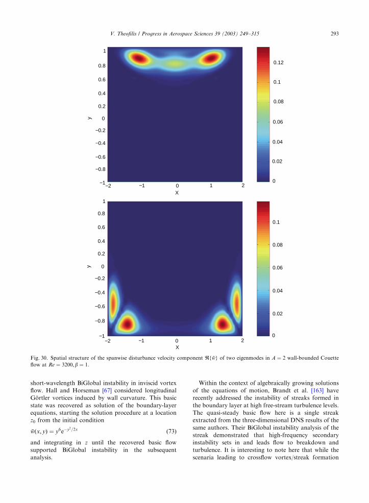
short-wavelength BiGlobal instability in inviscid vortex

flow. Hall and Horseman [67] considered longitudinal

G .ortler vortices induced by wall curvature. This basic

state was recovered as solution of the boundary-layer

equations, starting the solution procedure at a location

z0 from the initial condition

%wðx; yÞ ¼ y6e�y2=2x ð73Þ

and integrating in z until the recovered basic flow

supported BiGlobal instability in the subsequent

analysis.

Within the context of algebraically growing solutions

of the equations of motion, Brandt et al. [163] have

recently addressed the instability of streaks formed in

the boundary layer at high free-stream turbulence levels.

The quasi-steady basic flow here is a single streak

extracted from the three-dimensional DNS results of the

same authors. Their BiGlobal instability analysis of the

streak demonstrated that high-frequency secondary

instability sets in and leads flow to breakdown and

turbulence. It is interesting to note here that while the

scenaria leading to crossflow vortex/streak formation

1

0.8

0.6

0.4

0.2

0

−0.2

−0.4

−0.6

−0.8

−1

0.12

0.1

0.08

0.06

0.04

0.02

0

0.1

0.08

0.06

0.04

0.02

0

1

0.8

0.6

0.4

0.2

0

−0.2

−0.4

−0.6

−0.8

−1

yy

−2 −1 10 2

−2 −1 10 2X

X

Fig. 30. Spatial structure of the spanwise disturbance velocity component Rf *wg of two eigenmodes in A ¼ 2 wall-bounded Couette

flow at Re ¼ 3200;b ¼ 1:


35

30

25

20

15

10

5

00 5 10 15 20 25 30 35

ζ

η35

30

25

20

15

10

5

0 5 10 15 20 25 30 35ζ

η35

30

25

20

15

10

5

0 5 10 15 20 25 30 35ζ

η35

30

25

20

15

10

5

0 5 10 15 20 25 30 35ζ

η

35

30

25

20

15

10

5

0 5 10 15 20 25 30 35ζ

η

35

30

25

20

15

10

5

0 5 10 15 20 25 30 35ζ

η

(e) (f)

(e) (f)

(e) (f)

Fig. 31. Spatial structure of the real (left column) and imaginary (right column) parts of the streamwise disturbance velocity

component #w of the three most unstable viscous eigenmodes in corner flow instability as function of the transformed x and y

coordinates, z and Z; respectively [72], Upper to lower, modes I, II and III.


are fundamentally different, flow turbulence in both

cases originates through a qualitatively analogous

mechanism which can be described by BiGlobal linear

theory.

4.9. The wake–vortex system

4.9.1. Basic flow models

In the course of current efforts to minimise the

extent and strength of coherent vorticity in the wake

of passenger aircraft during take-off and approach,

the subject of instability of systems of trailing vortex

models has received renewed attention. Since the

key objective of the current efforts is to provide

recommendations leading to reduction of aircraft-

separation limits, currently of the order of a few

minutes, focus of instability analyses is on mechanisms

other than the classic Crow [44] instability, the long-

wavelength nature of which excludes it from playing an

active role in the sought process. Rather than the single

pair of counter-rotating or co-rotating vortices, the

stability of which has respectively been addressed by

Crow [44] and Jim!enez [164] attention is currently

focussed on systems of multiple vortices produced by a

flaps-down configuration. These flows can be modelled

by linear superposition of isolated vortex tubes of

prescribed circulation as schematically depicted in

Fig. 32; however injecting such a system into the

governing equations in general does not deliver a steady

or time-periodic basic state in the sense of Section 2.

Experimentation and numerical simulation are indis-

pensable to understanding the basic flow character in

this problem.

de Bruin et al. [45] have measured the (three-

dimensional) wake behind a commercial aircraft model;

assuming that the turbulence level in the wake was low,

they used the two-dimensional field at a specific down-

stream location in the axial direction of the aircraft

motion, z; as input for two-dimensional DNS calcula-

tions based on (16) and (17) and obtained very good

agreement between experiment and DNS calculation at

further downstream locations. The basic flow was found

to be a time-periodic state in which each pair of

starboard/port vortices rotates about the common

centroid. A different approach has been followed by

Rennich and Lele [165] who used the equilibrium

condition

b2

b1

� �3

þ3gG

b2

b1

� �2

þ3b2

b1

� �þ

gG

¼ 0 ð74Þ

to relate the circulations G; g and distances b1; b2 of the

vortices, taking advantage of the well-known fact that

satisfaction of (74) renders the configuration of Fig. 32 a

quasi-stationary solution of the equations of motion in

which the entire vortex system descends at a constant

speed. Moreover, it has been argued that configurations

having parameters which satisfy this equilibrium condi-

tion can be representative of a number of commercial

aircraft wakes.

4.9.2. Analysis, numerical solutions and the eigenvalue

problem

Crouch [46] addressed the instability of a basic flow

composed of two pairs of co-rotating vortices, taking the

first pair of signs for the circulation g in Fig. 32. He

employed the vortex-filament approach also used by

Crow [44] and Jim!enez [164] and numerical solutions of

the initial value problem resulting from matching the

induced velocities that the Biot–Savart law delivers with

kinematic conditions resulting from temporal differen-

tiation of the position vectors of the vortex system. The

elegance of this approach lies in that the stability

investigation may proceed analytically to a large extent.

Its drawback is that the instability results delivered are

relevant to the physical problem only for wavelengths

that are long compared to the core size of the vortices

and spurious instabilities may be predicted if this

condition is violated. Taking this condition into

consideration Crouch [46] proceeded by assuming that

b1

b2

2r1 2r2

Γ +/−γ −Γ−/+γ

Fig. 32. One global instability analysis concept in a trailing vortex system.


the helical motion of the vortex pair on either side of the

aircraft has a wavelength much larger than that of a

developing instability and thus time is the only para-

meter characterising the motion of each vortex pair in

the basic state; the periodic motion was treated by

Floquet theory.

Three different instability mechanisms were discov-

ered by Crouch [46]; they are depicted in Fig. 33 after

one period of their respective evolution. The first is akin

to Crow instability and corresponds to wavelengths and

growth rates that are, respectively, too large and too

small to be interesting for the wake–vortex minimisation

problem (top of figure). The second mechanism corre-

sponds to a new class of symmetric and antisymmetric

disturbances (as viewed from the ground), which were

discovered at shorter wavelengths, having growth rates

up to twice as large as those of the Crow-like instabilities

(middle of figure); as such, these instabilities may have

an active role to play in the problem at hand. However,

the third physical mechanism, transient growth of the

wake–vortex system, has been identified to be the most

promising one to be exploited for early breakdown of

trailing vortices in the problem at hand. While this well-

established in channel flows [166,167] route to transition

is inactive at short wavelengths (scaling with the vortex

spacing), at large wavelengths and/or when one vortex

pair only is excited, it yields growth rates which can be

an order of magnitude larger than those delivered by

linear theory, leading the wake–vortex system to lose its

coherence in a fifth of the time that the strongest of the

linear mechanisms of the previous two types may do.

Physically founded instability mechanisms have been

experimentally verified on realistic wing configurations

(Crouch, personal communication) as part of the effort

of transitioning this theoretical knowledge to systems

for wake–vortex control of commercial airliners.

Fabre and Jacquin [47] addressed a configuration

composed of two pairs of counter-rotating vortices (i.e.

considered the second pair of signs for g in Fig. 32)

subject to (74), which determines the positioning of the

vortices once circulation is specified, i.e. modelled from

experiment. These authors also used a vortex filament

method for the instability analysis and complemented

their linear theory by a transient growth study. In the

case of a system of counter-rotating vortices too, linear

instabilities additional to the Crow mode were discov-

ered; the dependence of the (scaled) growth rates on

wavenumber is shown in Fig. 34. The analogon of the

Crow instability is denoted by the second symmetric

mode S2, while it can be seen that the discovered modes

S1 and A are respectively amplified by factors 10 and 5

stronger than S1; the spatial structure of the new

eigenmodes is shown in Fig. 35. While interesting in

their own right, these instabilities, of the classic elliptic

nature first discussed theoretically by Pierrehumbert [10]

and Bayly [86], they contribute little to the modification

of the (stronger) outer vortices and attention must be

focussed on mechanisms other than their BiGlobal

linear instability in order to address the wake–vortex

minimisation problem; work is in progress on this issue.

The restrictions of the vortex-filament approach and

those implied by (74) may be relaxed when solving the

two-dimensional eigenvalue problem (28)–(31). Jacquin

et al. [93] have discussed applicability of the BiGlobal

instability analysis concept by analysing basic flow

systems constructed by linear superposition of pairs of

co-rotating and counter-rotating Batchelor-like vortices

t = T

t = T

t = T

Fig. 33. Modification of the wake–vortex system on account of

the mechanisms discussed by [46].


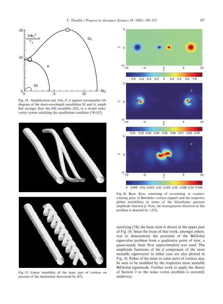
satisfying (74); the basic state is shown in the upper part

of Fig. 36. Since the focus of that work, amongst others,

was to demonstrate the potential of the BiGlobal

eigenvalue problem from a qualitative point of view, a

quasi-steady basic flow approximation was used. The

amplitude functions of the #p component of the most

unstable eigenvector in either case are also plotted in

Fig. 36. Either of the inner or outer pairs of vortices may

be seen to be modified by the respective most unstable

BiGlobal eigenmode. Further work to apply the theory

of Section 2 to the wake–vortex problem is currently

underway.

18

10

00 5 10

A

S2

S12πb1

2

Γ1σ

kb1

Fig. 34. Amplification rate 2pb1=G1s against wavenumber kb1

diagram of the short-wavelength instabilities S1 and A, ampli-

fied stronger than the [44] instability (S2), in a model wake–

vortex system satisfying the equilibrium condition (74) [47].

Fig. 35. Linear instability of the inner pair of vortices on

account of the mechanism discovered by [47].

5

0

−5−10 0−5 5 10

y

z

0.80.4 0.60.20−0.2−0.4−0.6−0.8

5

0

−5−10 0−5 5 10

y

z

0.090.07 0.080.060.050.040.030.020.015

0

−5−10 0−5 5 10

y

z

0.0450.035 0.040.030.0250.020.0150.010.0050

Fig. 36. Basic flows consisting of co-rotating or counter-

rotating pairs of Batchelor vortices (upper) and the respective

global instabilities in terms of the disturbance pressure

amplitude function #p: Note, the homogeneous direction in this

problem is denoted by z [93].


4.10. Bluff-body instabilities

4.10.1. Laminar flow past a circular cylinder

Bluff-body instability and transition is one problem in

external aerodynamics, full understanding of which

should, in the author’s view, precede theoretically

founded flow control methodologies. Insight into bluff-

body three-dimensional instability has been gained by

substantial progress made in the elementary configura-

tion of an infinite cylinder from both an experimental

[168] and a theoretical/numerical point of view, the

latter employing accurate spectral-element DNS meth-

odologies [169,23,24]. The linear stages of the transition

process on the cylinder are now reasonably well-under-

stood. A Hopf-bifurcation above a Reynolds number

Re ¼ UND=nE47; establishes a time-periodic nominally

two-dimensional state of the form (26) in which two-

dimensional vortices having their axes parallel to that of

the cylinder are shed. The Hopf bifurcation itself can be

associated with instability of the ðb ¼ 0Þ-BiGlobal

eigenmode superimposed upon the laminar two-dimen-

sional steady-state circular cylinder solution prevailing

at Reo47: The instability of the time-periodic state is

subsequently sought by Floquet theory. Barkley and

Henderson [24] and Henderson and Barkley [23] have

made essential contributions by identifying two distinct

mechanisms, visualised in Fig. 37. Mode A instability

sets in at Re ¼ 189 and corresponds to a spanwise

wavelength Lz ¼ 2p=bE4D; mode B instability is

encountered at Re ¼ 259 and has a characteristic

wavelength of the order of the cylinder diameter; the

spatial structure of both can be seen in Fig. 38. While

the BiGlobal linear problem of circular cylinder

instability may be considered closed, the nonlinear

development of the BiGlobal eigenmodes A and B,

including the question of energy transfer between them

as the Reynolds number increases has continued

receiving attention [23,61]. The earlier modelling efforts

of Noack and Eckelmann [170] and co-workers as well

as recent renewed efforts of the same investigators are

also noted in this respect.

4.10.2. Laminar flow past a rectangular corrugated

cylinder

The envelope of bluff bodies the linear and nonlinear

instability of which has recently been studied was

enlarged by the DNS-based analyses of Darekar and

Sherwin [171]. These authors considered a cylinder of

rectangular cross-section of base-height D on the Oxy

plane, the corrugation of which was determined by a

wavelength Lz in the z-direction and a peak height of

the waviness Wx: The essential generalisation that

the specific geometry offers compared with that of the

circular cylinder is the introduction of three-dimension-

ality, determined by the independent parameters Wx=Lz

and Lz=D: The underlying experimental observation for

this and analogous geometries has been that corrugated

cylinders have distinct advantages over the circular

cylinder geometry in terms of suppression of vortex

shedding and drag reduction [172]. While experiments

were performed at Re ¼ 4 � 104 a spectral=hp element

methodology was used for computations at Rep150;

A

BRe*2

Re2

6

4

2

0200 250 300

Re

λ =

2π

/ β

Fig. 37. Neutral loops of global Mode A and B instabilities in

the wake of a circular cylinder [24].

Fig. 38. Mode A (upper) and B (lower) instability in the wake

of a circular cylinder [197].


based on cylinder-base height, after the corrugated

geometry was mapped onto a rectangular cartesian grid.

The Reynolds numbers chosen for the computations

ensured full resolution of the numerical results obtained

but at the same time revealed previously unknown

BiGlobal instability mechanisms at different flow

regimes.

At a constant Lz=D value these regimes are classified

as I, II (A) and (B) and III (A) and (B). In regime I the

principal effect of the corrugation is a weak three-

dimensionalisation of the K!arm!an vortex street. An

increase in the peak-waviness height leads to a regime II

(A) where a drastic decrease in the lift and a milder one

in the drag coefficient is observed. Simultaneous increase

of the parameter Lz=D; leads to regime II (B) which is a

combination between the previous two, the lift and drag

coefficients saturating in a time-periodic state with a

low-frequency modulation. Returning to the original

value of the parameter Lz=D and increasing Wx=Lz

further, regimes III (A) and (B) are reached, in the first

of which the lift coefficient is reduced to zero and the

drag coefficient attains its minimum value, while in

regime III (B) a small nonzero lift is produced and the

drag also increases by a few percent over that prevailing

in regime III (A). The key qualitative characteristics of

the wake in the three regimes are, respectively, two-

dimensionality, transitional flow and complete suppres-

sion of vortex shedding. Perspective views of the

different regimes in the wake behind the corrugated

cylinder are shown in Fig. 39.

The DNS computations of [171] rather than covering

the entire parameter space, a task practically impossible

using DNS, serve as a challenge for a quasi-three-

dimensional extension of BiGlobal linear instability

theory. Progress could be made by exploiting analytical

introduction of three-dimensionality, as done in the

computations of [171]; on the other hand, the potential

practical benefits from a detailed exploration of para-

meter space and the associated increase of the predictive

capacity of methodologies aiming at drag-reduction of

bluff-body configurations render such an extension of

the BiGlobal linear instability theory highly desirable.

Such an extension will also provide impetus to analyses

of flows at substantially higher Reynolds numbers

compared with those in [171], a task practically

impossible by use of DNS.

4.11. Turbulent flow in the wake of a circular cylinder

and an aerofoil

The progression from laminar flow on the unswept

circular or rectangular cylinder towards flight Reynolds

numbers highlights one of the most commonly encoun-

tered problems of flow on aerofoils at these conditions,

that of transitional or turbulent flow separation. Large-

scale cellular structures are long known to be associated

with this phenomenon [173] which has received a fair

amount of attention and interpretations; a qualitative

depiction is shown in the upper part of Fig. 40 [174].

Arguments have been put forward in the literature, that

these cellular structures may be related with end-effects

of the measurement section; such arguments can be

dismissed on account of the repeatability of the

phenomenon shown in Fig. 40 with varying spanwise

extent of the measurement domain, both in the case of

the cylinder and that of the aerofoil. One conjecture was

put forward by Goelling [174] on the basis of his

experimental results on the cylinder, namely that these

structures point to a BiGlobal instability mechanism.

y

xz

y

xz

yx

z

(b)

(c)

(b)

Fig. 39. Visualisation of r!egimes I (upper), II-B (middle) and

III-B (lower) in the wake of a corrugated cylinder [171].


Experimental findings in support of this conjecture

are the following. On a qualitative level, the two-

dimensional closed separation bubble on the unswept

cylinder first becomes spanwise unsteady with increasing

Re; the related spanwise periodic vortical cellular

structure appearing as a result is shown in the lower

part of Fig. 40. Associated is the formation of K!arm!an-

like vortices, having their axes parallel to the generator

of the cylinder, while up to this point the same

qualitative scenario is followed on the aerofoil. The

topological description of one of the spanwise periodic

cells at the upper side of the cylinder is shown in the

lower part of Fig. 40; a pair of streamwise vortices

separates from one of these cells, either from the cylinder

or from the aerofoil at comparable flow parameters. On

a quantitative level Humphreys [173] has argued that the

spanwise periodicity length Lz of the structures on the

circular cylinder scales with its diameter D: In flow

visualisations he found Lz=DA½1:7; 2:4: In recent

experiments Goelling [174] confirmed this bracket at

corresponding Re values and showed that an increase of

Reynolds number decreases the spanwise periodicity

ϕDr = 135 Grad

ϕDr = -135 Grad

0°

0°

b

ac

d

e

95f

95 Grad

105 Grad

140 Grad

180 Grad

Fig. 40. Upper: symmetric cellular structures arising in transitional flow on a circular cylinder [174]. Lower: detailed view of one of the

structures and sketch of its topological characteristics.


length to LzED: Interestingly, this progression is not

continuous; this is interpreted as a hint of amplification

of different BiGlobal eigenmodes as Re increases.

The link to the BiGlobal instability scenario discussed

in Section 4.10.1 is provided by the shear-layer which

engulfs the wake-region within which the unstable

BiGlobal ‘‘B’’ mode develops and flow outside the

cylinder wake [175]. With increasing Reynolds number

the laminar shear-layer emanating from the cylinder

surface becomes unstable and turbulent, whereby

transition is associated with the appearance of small-

scale streamwise-oriented turbulent vortices [176,177].

The transition point moves upstream as the Reynolds

number increases above Re 5 �B103: It has been

conjectured [174] that the interaction of the laminar

boundary-layer at the cylinder surface with the unsteady

flowfield in the near-wake is the reason for the

appearance (through a BiGlobal instability mechanism)

of the large-scale spanwise periodic structures on the

cylinder surface itself. Such structures have also been

observed by Schewe [178–180] on his generic aerofoil

experiment, with periodicity lengths in the same range as

on the cylinder at comparable conditions, as seen in

Fig. 41. Whether this mechanism can be described in the

framework of a BiGlobal linear instability of separated

flow or bluff-body instability deserves further investiga-

tion. In case of the absence of a steady or time-periodic

laminar two-dimensional basic state underlying a

BiGlobal instability analysis in the problem at hand,

one may employ the recently developed and successfully

applied to one-dimensional instability problems triple-

decomposition methodology of Reau and Tumin [181].

Flow

Re = 7.4 × 105 CD = 0.11 CL = 1.1

CL = 0.65CD = 0.14Re = 7.7 × 106

Re = 0.32 × 106 CL = 0.50 CD = 0.50

CL = 1.52 CD = 0.02

CL = 1.20 CD = 0.13

CL = 0.79 CD = 0.15

Re = 0.80 × 106

Re = 1.2 × 106

Re = 7.4 × 106

subcritical

supercritical

step region

transcritical

Fig. 41. Upper: asymmetric cellular structures in transitional flow over an aerofoil [180]. Lower: topological characteristics of the cell

structures.


The connection of the topological features in the present

flow with those in the BiGlobally unstable laminar

separation bubble on an aerofoil, discussed earlier,

including mechanisms for vortex shedding from cylin-

ders and aerofoils also deserves investigation in the

framework of the present theory.

4.12. On turbulent flow control

The scope of the discussion of the previous section can

be naturally broadened to incorporate the broader field

of turbulent separated flow control. The reader is

referred to the recent milestone review of this problem

by Greenblatt and Wygnanski [25] who highlighted the

potential of periodic excitation, i.e. oscillatory momen-

tum injection as effective and efficient means of flow

control, irrespective of the latter being found in a

laminar, transitional or turbulent state. Based on

overwhelming amounts of experimental information

Wygnanski and co-workers ([182–185,25] and references

therein) arrived at the conclusion that periodic excita-

tion can be more efficient for certain airfoil applications

than classic boundary-layer control methodologies

based on steady suction/injection and provided two

key parameters to quantify excitation.

The amount of injected flow was referred to free-

stream conditions to arrive at the momentum coefficient

Cm ¼rU2

j G

12rN

U2N

L; ð75Þ

where G denotes a characteristic length associated with

the excitation, e.g. a slot width, Uj is the magnitude of

the injected velocity and L ¼ Oð1Þ is the length of the

body in consideration, e.g. the length of the separation

region, for simplicity taken to be the chord length of an

aerofoil [182]. The actuation itself is characterised by a

reduced frequency

Fþ ¼feX

UN

; ð76Þ

where X is a distance from the location on the body

surface at which excitation is provided to the end of the

body (or the natural reattachment point) in question and

fe is the excitation frequency. The underlying theme of

the experimental work in this group is that efforts must

be directed towards utilising the natural flow instability,

enhanced by the periodic addition of momentum at the

appropriate location, magnitude and frequency to

interact with the large-scale coherent structures of

the flow.

In the case of turbulent flow it is found that the most

effective oscillation frequencies of the periodic forcing

are widely disparate from those of turbulence; further-

more, it is proposed to monitor the dependence of the

reduced frequency in conjunction with the momentum

coefficient. Nishri and Wygnanski [186] proposed a

generic deflected flap configuration as an example on

which the controlling parameters could be isolated and

discovered that practically independently of Reynolds

number

FþB1 ð77Þ

is the optimum reduced frequency for control of

turbulent separated flow, independently of the level of

free-stream turbulence [183,184]. This suggests that

structures scaling with the separation bubble length

itself, and not the order-of-magnitude smaller TS-

wavelengths associated with shear-layer instability, are

being modified by a reduced frequency (77) a result that

may be pointing to the BiGlobal eigenmodes structure

shown in Fig. 15. The result that Fþ ¼ Oð1Þ has been

corroborated in a multitude of turbulent separated flow

control experiments [25] and its potential association

with a generic BiGlobal instability mechanism is worthy

of further investigation.

4.13. Analyses based on the linearised Navier–Stokes

equations (LNSE)

Finally, as an exception to the main focus of the

present paper on incompressible flows, a short discus-

sion of the recent efforts of Collis and Lele [53] and

Malik [54] in subsonic and hypersonic boundary layer

flow stability, respectively, is provided. Both approaches

use the (compressible) LNSE concept to study the

problems of receptivity [62] and subsequent linear and

nonlinear instability of boundary-layer (its instability

per se being amenable to analysis based on the PSE) in a

unified manner. One motivation provided by current

practitioners of the LNSE approach is that while the

nonlinear PSE provides a complete framework to study

nonparallel and nonlinear phenomena in boundary-

layer transition, question of receptivity, i.e. the accurate

description of the process by which disturbances enter

the boundary layer, cannot be tackled by PSE and even

less so by OSE-based analyses; this problem is circum-

vented by use of the linearised Navier–Stokes equations.

A point in this case was the work of Collis and Lele

[53] who considered the leading-edge region of a swept

wing including an analytically described roughness

element. Their work was placed within the framework

of laminar-flow wings and receptivity of the flow to the

introduced roughness was the main issue addressed.

Technical details are omitted here and may be found in

the original reference. Key results were provided by

comparison of parallel-flow predictions and the LNSE;

it was noted that nonparallel and curvature effects

counteracted each other, but nonparallel effects domi-

nated the configuration studied and strongly reduced the

initial amplitude of the crossflow vortices developing on

the wing surface compared with one-dimensional theory

predictions. The implication is that, in the absence of the


LNSE predictions, a PSE-based analysis of crossflow

vortices on the specific configuration would produce

inaccurate results on account of wrong initialisation of

the computations.

Malik [54], on the other hand, employed two-

dimensional LNSE to study stability of a Mach 8 wedge

flow. The domain considered was bounded by a solid

wall with a suction slot, a shock on which appropriate

conditions were imposed, an inflow boundary near

but not at the wedge tip, at which appropriate

inflow boundary conditions were imposed and a

buffer-domain outflow boundary at which, in a manner

analogous with spatial DNS, disturbances were

artificially reduced to zero. Inside the domain thus

defined the compressible analogon of the two-dimen-

sional limit of (20)–(24) was solved, the key difference

from solution of the two-dimensional ðb ¼ 0Þ BiGlobal

EVP being the relaxation of the assumption of harmonic

disturbances on time. Disturbances were introduced into

the flow by localised wall suction/blowing. Key result of

this work has been the generation of fast and slow

acoustic modes and the subsequent dominance of second

mode instability, in line with the predictions of one-

dimensional linear theory and earlier spatial DNS

of Mach 4.8 boundary layer flow of Eissler and Bestek

[187]. The potential of LNSE instability analyses

of essentially nonparallel basic flows and its

potential synergy with the BiGlobal EVP have not been

exploited yet.

5. Discussion and research frontiers

The present review has emerged as an attempt to

summarise recent theoretical developments in the field of

linear instability of essentially nonparallel flows of

relevance to aeronautics. Both open and closed systems

were considered, having the unifying characteristic of a

basic state that is inhomogeneous in two and periodic in

the third spatial direction. The scope has been narrowed

by focussing mainly on solutions of the two-dimensional

eigenvalue problem which describes linear instability of

such nonparallel flows. Since the classic review of

Huerre and Monkewitz [7] at the latest, the term ‘global’

flow instability has been used in a different context too.

In this review, the term ‘global’ has been synonymous

with instability of nonparallel basic flows; further, the

more precise notion of ‘BiGlobal’ instability analysis has

been introduced to denote the essential two-dimension-

ality of the corresponding basic state. This definition

may encompass that of work in the vein of [7] in that

‘absolute/global’ instability in the latter methodology

may be related, in principle, with instability of the two-

dimensional ðb ¼ 0Þ global eigenmode in the present

terminology in certain limiting cases. However, no work

is known at present explicitly linking the two approaches

although such a link may exist as evidenced by the

qualitative consistency of the independently produced

results of the two analysis approaches on the only

problem on which they have been concurrently applied,

that of global instability of a separation bubble,

discussed herein.

The historical evolution of approaches for the

formulation and numerical solution of the BiGlobal

instability EVP has followed the rapid developments in

computing hardware as well as those in efficient

algorithms for the linear algebra of large matrices. Born

in the late 1980s, the BiGlobal EVP initially focussed on

the inviscid generalised Rayleigh equation applied to an

analytic two-dimensional basic state, which from a

numerical point of view requires the recovery of a single

two-dimensional eigenfunction. The theory progressed

into the viscous regime, where the generalised Orr–

Sommerfeld and Squire coupled system was solved for

the recovery of two-dimensional eigenfunctions. In the

early work, the classic QZ algorithm has been used for

the recovery of the eigenspectrum. Its limitations were

quickly appreciated so that currently efficient Krylov

subspace iteration methods are almost exclusively used.

These permit addressing the incompressible/compressi-

ble two-dimensional EVP in primitive-variables formu-

lation, requiring simultaneous solution of systems for

the recovery of four/five two-dimensional eigenfunc-

tions, respectively. A key observation in this evolu-

tionary process of the methodologies for the numerical

solution of the two-dimensional EVP has been the

consistent failure of second-order accurate numerical

methods to deliver reliable global instability results; for

the problem at hand, in which resolution cannot be

increased beyond hardware-limited bounds, a high-

order method (spectral/finite element, spectral colloca-

tion, compact finite-difference) is in the author’s view

indispensable.

Alternative methodologies for the solution of the two-

dimensional eigenvalue problem exist for the recovery of

BiGlobal instability results. DNS may, in principle, be

employed, though at a larger computing cost and,

potentially, at the expense of information on members

of the eigenspectrum other than the most unstable/least

stable eigenmode going unnoticed. If applicable on

physical grounds, a combination of Floquet analysis in a

homogeneous spatial direction with one-dimensional

EVPs in the second resolved inhomogeneous direction

may be employed. If sufficient computing power is

available but the overhead of DNS is deemed to be too

high, developing and maintaining a Floquet/1D-EVP

code may not be justified compared with a straightfor-

ward two-dimensional EVP in which the homogeneous

spatial direction is treated by a discrete Fourier

expansion. Yet another alternative for global instability

analysis, that of LNSE, is slowly emerging in the

literature.


The ability to address the numerical aspects of global

instability analysis in an adequate manner does not

necessarily imply that the results obtained are also

adequate from a physical point of view. Consistent with

the failure of the one-dimensional limit of linear theory

on the corresponding problem, global linear analysis of

wall-bounded Couette flow has not delivered unstable

eigenmodes. This paradox is thus added to that of a duct

of square cross-section and to the best-known failure of

one-dimensional linear theory, Hagen–Poiseuille flow in

a circular pipe. In other applications mixed success has

been obtained: the discovery of new global eigenmodes

in the swept attachment line boundary layer, or that in

the rectangular duct, is not sufficient to explain the

respective subcritical instability problems, although the

BiGlobal eigenmodes of the first problem are essential

building blocks of theoretical approaches which address

the (nonlinear) physical problem successfully. On the

other hand, BiGlobal linear instability analysis has also

delivered spectacular successes in its own right. In-

stability in the wake of cylinders of circular or

rectangular cross-section is one paradigm, as is flow in

the long-standing numerical benchmark of the lid-driven

cavity. Instability of separated flow is another example

where application of global linear theory has delivered

new physical insight into an old problem of external and

internal aerodynamics.

For the most part, however, the field of potential

applications of BiGlobal linear theory in aeronautics is

wide open with an associated large potential for

improvement of current understanding of flow physics.

BiGlobal instability of vortical flows on lifting surfaces

or the wake–vortex system has only started being

examined by this general concept and already first

successes have been reported (cf. crossflow vortices,

G .ortler vortices, streaks). The applicability of the

concept on the entire aerofoil has commenced but much

work needs to be done, not least from the point of view

of algorithmic developments. In the latter respect,

development of global flow methodologies on unstruc-

tured grids could come to bear both in the problem of an

aerofoil and in that of blade configurations in turbo-

machinery. Open cavity instability research might profit

from investigations into scenarios other than the

empirical Rossiter mode, especially in view of the (far

from idealised shear-layer) flowfield in three-dimen-

sional cavities with/without stores. Corner flows, in

which the issue of the basic flow itself is far from being

settled, is another configuration in external aerody-

namics, for which BiGlobal instability theory could

prove beneficial and should be pursued further.

Progress in BiGlobal instability theory could be

viewed as the advancing of knowledge stemming, firstly,

from revisiting with the new methodology many of the

idealised flows the linear instability of which has been

addressed using one-dimensional analysis in the last

century and, secondly, by solving problems of industrial

significance, the instability of which cannot be addressed

by classical means. BiGlobal instability analysis has

been shown to encompass the results of classic linear

theory either at appropriate limits (e.g. duct flows at

A-N) or as part of the two-dimensional eigenvalue

problem solution (c.f. attachment-line boundary layer,

corner flows and open cavity results discussed herein)

such that linear theory in future work may in principle

focus on the two-dimensional eigenvalue problem alone.

A different point of view on progress comes from the

realisation of some essential problems in aeronautics.

From a numerical point of view, most applications

involve complex geometries for the resolution of which

the tensor-product grids currently used by a BiGlobal

analysis on canonical grids are either not optimal or

entirely inappropriate. Efficient adaptive-grid algo-

rithms are known in aeronautics for a long time;

however, their accuracy properties may be inferior to

those required by a global instability analysis (or,

indeed, DNS); progress could result from designing

flexible, efficient and accurate numerical algorithms for

the two-dimensional EVP. Further progress from a

physical point of view, on the other hand, could result

from incorporation of inhomogeneity of the third spatial

direction in the analysis. Specifically, an intrinsic

difficulty of several applications in aeronautics is three-

dimensionality of the underlying basic flowfields (e.g.

vortical flows or the corner boundary layers discussed

herein). These are approximated in current analyses

(including some employing DNS) by an assumption

equivalent to the parallel-flow approximation in bound-

ary layers, although such an assumption is not permitted

on physical grounds. One potentially interesting exten-

sion of global linear theory could enlarge the scope of

current analysis based on the two-dimensional eigenva-

lue problem and address mild three-dimensionality in

the third spatial direction by means more efficient than a

DNS in which all three spatial directions are taken to be

inhomogeneous, or the three-dimensional (TriGlobal)

EVP.

Last but not least, the time may now be ripe to revisit

the issue of ‘coherent structures’ of turbulent flow. This

issue became popular in past decades before interest

subsided in the absence of a convincing breakthrough

delivered by approaches focussing on coherent struc-

tures compared with more traditional turbulent flow

research methodologies. It should be stressed, however,

that the structures discussed in the past were for the

most part a result of post-dicting an existing flowfield. A

key new element offered by global instability theory is

the a priori knowledge of the global eigenmodes of a

three-dimensional flowfield and its exploitation, for

example in the framework of nonlinear global instability

analyses, to advance understanding of their relation

to turbulent flow structures. The potential benefit for


effective flow-control methodologies that such an

understanding could deliver is, in the author’s view,

worthy of exploration.

Acknowledgements

This work was initiated by an Alexander von

Humboldt Research Fellowship and partly supported

by the European Office of Aerospace Research and

Development under contracts monitored by C. Raffoul.

His active interest as well as interactions with several

colleagues over the last years, notably P.W. Duck

(University of Manchester), U. Dallmann, W. Koch

and S. Hein (DLR), S.J. Sherwin (Imperial College),

E. Janke (BMW/Rolls-Royce), T. Colonius (Caltech),

R.L. Kimmel and M. Stanek (Wright-Patterson AFB),

are gratefully acknowledged.

Appendix A

With ever increasing computing hardware capabilities

the list of flows of aeronautical interest whose global

instability is addressed numerically increases steadily. In

the cases studied so far, experience has shown that

substantial discrepancies in the instability analysis

results can occur on account of insufficient attention

being paid to the issue of the basic flow. The set of

algorithms which follow have been used for the recovery

of basic flows relevant to external aerodynamics in

closed and open systems, and shown to satisfy the key

requirement of global instability analysis to deliver

results of optimal quality on a modest number of

discretisation points.

A.1. A spectral-collocation/finite-difference algorithm for

the numerical solution of the nonsimilar boundary layer

equations

In this case length, time and velocity scales may be

built,

L ¼ b0=b1; T ¼ 1=b1; and b0; ðA:1Þ

respectively, defining a Reynolds number

Re ¼b0L

n: ðA:2Þ

The dimensional independent variables x and y may

be transformed into dimensionless boundary-layer vari-

ables, x and Z; according to

x ¼b1

b0

x; and Z ¼b1

b0

ffiffiffiffiffiffiRe

2x

ry: ðA:3Þ

A streamfunction may be defined through

cH ¼ffiffiffiffiffiffiffiffiffiffiffiffiffiffiffi2b0nLx

pf ðx; ZÞ ðA:4Þ

and the velocity components of the Howarth boundary

layer flow, uH and vH; take the form

uH ¼@cH

@y¼ b0

@f

@Zand

vH ¼ �@cH

@x¼ �

ffiffiffiffiffiffiffib1n2x

sf þ 2x

@f

@x� Z

@f

@Z

� �: ðA:5Þ

The steady boundary layer equation

uH@uH

@xþ vH

@uH

@y¼ Ue

dUe

dxþ n

@2uH

@y2ðA:6Þ

is then transformed into

@3f

@Z3þ f

@2f

@Z2þ 2x

@f

@x@2f

@Z2�

@f

@Z@2f

@x@Z

� �¼ 2xð1 � xÞ: ðA:7Þ

This nonsimilar boundary layer equation constitutes a

parabolic problem which may be marched in x: The

boundary conditions in Z are no penetration and no-slip

at the wall and (19) in the free-stream,

f ðZ ¼ 0Þ ¼ 0; ðA:8Þ

@f

@ZðZ ¼ 0Þ ¼ 0; ðA:9Þ

@f

@ZðZ-NÞ ¼ 1 � x: ðA:10Þ

The vorticity of the flow is given by

zH ¼ r2cH ¼b1ffiffiffiffiffiffiffiffiffiffiffiffiffi8x3Re

p �f þ 4x@f

@xþ 4x2 @

2f

@x2þ 2Z

@f

@Z

�

� 4xZ@2f

@x@Z� Z

@f

@xþ Z2 @

2f

@Z2þ 2xRe

@2f

@Z2

�:

ðA:11Þ

A numerical solution of (A.7) subject to boundary

conditions (A.9) and (A.10) has been the subject of

intense investigation in the past with respect to the

appearance of the singularity in the solution and the

determination of the abscissa for separation [136]. A

simple modification of the boundary layer equations

which takes the interactive nature of the boundary layer

into account [138] succeeds in closely reproducing the

results obtained by solution of the Navier–Stokes

equations [137].

The nonsimilar boundary layer equations constitute a

parabolic problem which may be solved by marching in

the x direction. This is discretised by a grid of uniform

spacing Dx: In the wall-normal Z-direction the optimal

resolution properties of a spectral expansion are

exploited. Spectral methods have been applied to the

solution of the boundary-layer equations by Streett et al.

[188] who transformed the problem (A.7) using G .ortler

variables. Here, at each x-station we solve (A.7) by


Newton-Kantorowitz iteration, in boundary-layer vari-

ables, in a manner analogous to that used by Theofilis

[52] for the generalised Hiemenz boundary layer.

Specifically, we define

*u ¼@f

@Z� Df ; ðA:12Þ

*v ¼ f ; ðA:13Þ

which transforms (A.7) into the system

D2 *u þ *vD *u þ 2x D *u@*v

@x� *u

@ *u

@x

� �¼ 2xð1 � xÞ; ðA:14Þ

*u �D*v ¼ 0; ðA:15Þ

subject to the boundary conditions

*uð0Þ ¼ *vð0Þ ¼ 0; and *uðZ-NÞ ¼ 1 � x: ðA:16Þ

A standard Newton procedure follows, writing

*uðnÞ ¼ *uðoÞ þ D *u; ðA:17Þ

*vðnÞ ¼ *vðoÞ þ D*v; ðA:18Þ

while a second-order accurate backward-difference

scheme discretisation in x results in the problem

D2 þ *vðoÞ þxDx

ð3*vðoÞ � 4 %v þ %%vÞ� �

D

�

þxDx

ð�6 *uðoÞ þ 4 %u � %%uÞ� ��

D *u

þ D *uðoÞ þ 3D *uðoÞxDx

� �D*v

¼ �D2 *uðoÞ � *vðoÞD *uðoÞ

�xDx

½D *uðoÞð3*vðoÞ � 4%v þ %%vÞ

þ *uðoÞð�3 *uðoÞ þ 4 %u � %%uÞ

þ 2xð1 � xÞ; ðA:19Þ

D *u �DD*v ¼ � *uðoÞ þD *vðoÞ ðA:20Þ

to be solved at each station x for the Newton

corrections, with %u and %v the converged solutions at

x� Dx and %%u and %%v those at x� 2Dx; respectively.

Once the boundary-layer solution at a downstream

location on the plate has been obtained a variant of the

EVD algorithm discussed may be used in a DNS

context. System (16) and (17) is then closed by the

following boundary conditions for separated boundary

layer flow [137]

At the inflow boundary : c ¼ cH; ðA:21Þ

z ¼ zH; ðA:22Þ

At the top boundary : @c=@y ¼ F ðxÞ; ðA:23Þ

z ¼ 0; ðA:24Þ

At the outflow boundary : @2c=@x2 ¼ 0; ðA:25Þ

@2z=@x2 ¼ 0; ðA:26Þ

At the wall : c ¼ 0; ðA:27Þ

@c=@y ¼ 0; ðA:28Þ

where

F ðxÞ ¼b0 � b1x; xpx0;

b0 � b1x0; x > x0:

(ðA:29Þ

A full discussion of these boundary conditions may be

found in Briley [137]. In short, the boundary layer

solution (A.4) and (A.11) is used at the inflow boundary

x ¼ b0x=b1; the flow is taken to be irrotational at the

far-field boundary y-N where the free-stream velocity

distribution (A.29) is imposed, x0 being a free parameter

which determines the size of the recirculation region.

The outflow boundary conditions are satisfied to within

Oð1=ReÞ by the quantities @2c=@x2 and n @2z=@x2:Finally, (A.27) and (A.28) represent the physical

boundary conditions of no penetration and no-slip

at the solid wall. A subtle point worthy of mention here

is that the boundary condition for z based on the

Howarth boundary layer solution (A.11) is consistent

with that derived from the full Navier–Stokes equations,

zw ¼ @u=@yðy ¼ 0Þ; consequently no numerical instabil-

ity is expected to be generated owing to a singularity in

the boundary conditions at ðx ¼ xL; y ¼ 0Þ: This is

significant, especially in the context of numerical

solutions using spectral methods, since an incorrect

specification of boundary conditions in conjunction

with the absence of numerical dissipation may result

in propagation of the error and global numerical

instability.

Appendix B. An eigenvalue decomposition algorithm for

direct numerical simulation

The principles of the algorithm discussed in what

follows can be applied to recover three two-dimensional

velocity components or indeed a three-dimensional

flowfield [189]; however, for simplicity we confine the

present discussion to solutions of system (16) and (17)

which deliver a basic flowfield %q ¼ ð %u; %v; 0; %pÞT: It has

been mentioned that the main advantage of the velocity–

vorticity formulation is that the continuity equation is

exactly satisfied. However, the problem of imposition of

boundary conditions within the framework of an overall

efficient numerical solution algorithm remains. This is

compounded by the fact that the number of points

discretising the two spatial directions in the subsequent

analysis cannot be increased at will; while interpolation

of a basic flow solution obtained on a very large number


of points onto a modest EVP grid is one possible option,

it is more elegant to avoid the interpolation procedure

altogether and seek an accurate basic flow solution on

the same small number of discretisation points on which

the subsequent global instability analysis is to be

performed. This appears tailor-made for a spectral

numerical solution approach [100]. Ehrenstein and

Peyret [190] discussed one spectral algorithm for solving

(16) and (17) using the influence-matrix approach [191];

in what follows we discuss a different solution based

on an efficient real-space eigenvalue decomposition

(EVD) algorithm. Regarding spatial discretisation,

there is no restriction as to whether one or both spatial

directions x and y may be treated as periodic in the

basic flow problem; since aperiodic functions are

wider in scope and in line with the spirit of the present

two-dimensional linear instability analysis, we focus on

such solutions only.

Chebyshev polynomials have almost exclusively been

used in the past in the context of spectral simulations of

the time-accurate Navier–Stokes and continuity equa-

tions, mainly due to the availability of fast transform

algorithms necessary for efficient time-integration.

However, for the present problems we have not

restricted ourselves to this class of orthogonal poly-

nomials. Considerable freedom exists in the choice of the

expansion functions and the associated collocation grids

by using Jacobi polynomials Pðq;rÞ for the discretisation

of both spatial directions; of course, q ¼ r ¼ �0:5 may

be related to the Chebyshev—while q ¼ r ¼ 0 are the

Legendre polynomials. Collocation derivative matrices

for both Jacobi–Gauss–Lobatto and equidistant grids

can be constructed from first principles; if ðxj ; j ¼0;y; nÞ is the collocation grid chosen, the entries dij of

the ð0 : nÞ � ð0 : nÞ first-order derivative collocation

matrix D; derived analytically from the interpolating

polynomial [192], are

dij ¼Qn

k¼0ðxi � xkÞðxi � xjÞ

Qnk¼0ðxj � xkÞ

;

i; j; k ¼ 0;y; n; iajak; ðB:1Þ

dii ¼1Pn

k¼0ðxi � xkÞ; i; k ¼ 0;y; n; iak: ðB:2Þ

These formulae result in the well-known ones if the

analytically known Chebyshev–Gauss–Lobatto grid

ðxj ¼ cos jp=n; j ¼ 0;y; nÞ is used [193]. Values of

order m derivatives on the collocation grid xj are

obtained by ðDÞm:As far as temporal discretisation of (16) is concerned,

the viscous nature of the problems in which we are

interested introduces scales which dictate an implicit

treatment of the linear term in this equation; the

nonlinear term may be treated explicitly. Within the

framework of solution methods which do not resort to

splitting and introduction of intermediate fields but

rather address the governing equations directly the

combination of Crank–Nicholson (CN) with second-

order Adams–Bashforth (AB2) or Runge–Kutta (RK)

schemes has been extensively used for the time-integra-

tion of the viscous and the convective terms, respectively

[100]. However, the family of compact schemes pro-

posed by Spalart et al. [194] (SMR) presents more

accurate and more stable alternatives to the CN-AB2

algorithm although it does not require additional

computational effort to the latter scheme. The SMR

algorithm may be written in compact form as

q000 ¼ q00 þ DtfLiðkq00 þ lq000Þ þ mNlðq00Þ þ nNlðq0Þg;

ðB:3Þ

where the superscript denotes fractional time-step, LiðqÞand NlðqÞ are, respectively, the linear and nonlinear

operators in the problem to be solved and Dt is the time-

step. The rationale behind the derivation as well as

sample values of the constants k; l; m and n of a

self-starting SMR algorithm may be found in [194].

The time-discretisation of (16) using (B.3) delivers the

following problem to be solved for ðz;cÞ at each

fractional time-step

M1z000 ¼ R; ðB:4Þ

M2c000 þ z000 ¼ 0; ðB:5Þ

where M1 ¼ @2=@x2 þ @2=@y2 � Re=ðlDtÞ and M2 ¼@2=@x2 þ @2=@y2; subject to the boundary conditions

appropriate to the problem in consideration. R com-

prises the nonlinear and the terms arising from the

discretisation at previous fractional time-steps,

R ¼ � ðk=lÞ@2

@x2þ

@2

@y2� Re=ðkDtÞ

� �z00

þ ðmRe=lÞðc00yz

00x � c00

xz00yÞ

þ ðnRe=lÞðc0yz

0x � c0

xz0yÞ: ðB:6Þ

The accuracy of the overall procedure clearly depends

on the scheme utilised for calculation of the spatial

derivatives. The spectral discretisation chosen intro-

duces dense matrices and can only become competitive

against other numerical approaches from the point of

view of efficiency on account of the existence of a fast

algorithm for the inversion of the implicit operators M1

in (B.4) and M2 in (B.5). While M2 is time-independent,

the first implicit operator is a function of a CFL-

controlled maximum permitted time-step Dt and needs

to be inverted at every time-step. If one sacrifices the

advantage of an adjustable time-step and keeps Dt fixed

at a slightly lower than its optimal value, a powerful

EVD algorithm may be constructed for the efficient

solution of the incompressible two-dimensional Navier–

Stokes and continuity equations in streamfunction-

vorticity formulation.


Key papers on EVD algorithms are the work of

Haidvogel and Zang [195] and that of Ku et al. [189].

The first authors discuss the solution of Poisson’s

equation subject to homogeneous Dirichlet boundary

conditions in transform space while the second authors

present an eigenvalue decomposition algorithm for the

Poisson equation resulting from a time-splitting of the

incompressible Navier–Stokes and continuity equations

in primitive-variables formulation in the context of real-

space spectral collocation using Neumann boundary

data. Here we present a variant of the EVD algorithm

for the solution of the equations of motion in real-space

using the streamfunction-vorticity formulation. Using

this formulation within a direct, as opposed to time-

splitting or iterative, time-integration methodology one

Poisson and one Helmholz problem are to be solved

within each fractional time-step. This minimises the

necessary computing effort and makes the present

algorithm one viable candidate to obtain the desired

basic states.

Physical boundary conditions can only be provided

for the stream-function c itself and its derivatives on the

domain boundary. For the sake of exposure of the idea

in what follows the boundary conditions associated with

the standard testbed lid-driven cavity problem are

discussed. Further, we refrain from discussion of the

Ku et al. algorithm, which we term EVD2 for reasons

which will become apparent in what follows, and

concentrate on the EVD4 extension of the algorithm in

order to address problems in which both Dirichlet and

Neumann boundary conditions are imposed on the

stream-function while no boundary data are necessary

for the vorticity. We take the square lid-driven cavity

to be defined in the two-dimensional domain

ðxiA½0; 1; i ¼ 0;y;mÞ � ðyjA½0; 1; j ¼ 0;y; nÞ: The

boundary conditions on c are

cin ¼ c0j ¼ ci0 ¼ cmj ¼ 0; ðB:7Þ

ð@c=@yÞin ¼ F ðxiÞ; ðB:8Þ

ð@c=@xÞ0j ¼ 0; ðB:9Þ

ð@c=@yÞi0 ¼ 0; ðB:10Þ

ð@c=@xÞmj ¼ 0; ðB:11Þ

where fij � f ðxi; yjÞ represents either of c or z grid-

values at a fractional time-step and F ðxÞ is a function

used to distinguish between the classic singular lid-

driven cavity in which F ðxÞ ¼ 1 and a regularised [196]

cavity in which F ðxÞ ¼ 16x2ð1 � x2Þ: The numerical

discretisation of (B.4) and (B.5) leads to a system of

simultaneous equations of the type

Mf þ f N þ cIf ¼ g; ðB:12Þ

where M represents the ð0 : mÞ � ð0 : mÞ discrete analo-

gon of D2x; N represents the transpose of the ð0 : nÞ �

ð0 : nÞ discrete analogon of D2y; I is the identity matrix,

c ¼ �Re=ðlDtÞ and g ¼ R if (B.4) is being solved, while

c ¼ 0; g ¼ �z in the case of (B.5). On account of the

homogeneous boundary conditions (B.7) on c (B.5)

becomes

Xm�2

i¼2

Mkicil þXn�2

j¼2

Nljckj ¼ �zkl � Mk1c1l

� Mkm�1cm�1l � Nl1ck1 � Nln�1ckn�1: ðB:13Þ

The boundary conditions (B.8)–(B.11) may be expressed

using the discrete analoga X and Y of the collocation

derivative matrices Dx and Dy; respectively, as given by

(B.1) and (B.2). It follows that

c1l ¼Xm�2

i¼2

d1icil ; cm�1l ¼Xm�2

i¼2

dm�1icil ; ðB:14Þ

ck1 ¼ %kk þXn�2

j¼2

e1jckj ; ckn�1 ¼ %lk þXn�2

j¼2

en�1jckj ;

ðB:15Þ

where %kk and %lk are used to impose the boundary

condition on the lid,

%kk ¼�FkY0n�1

Y01Ynn�1 � Yn1Y0n�1;

%lk ¼FkY01

Y01Ynn�1 � Yn1Y0n�1ðB:16Þ

and the vectors d1i; dm�1i and e1j ; en�1j are known

functions of the entries of X and Y ;

d1i ¼X0m�1Xmi � Xmm�1X0i

X01Xmm�1 � Xm1X0m�1;

dm�1i ¼Xm1X0i � X01Xmi

X01Xmm�1 � Xm1X0m�1; ðB:17Þ

e1j ¼Y0n�1Ynj � Ynn�1Y0j

Y01Ynn�1 � Yn1Y0n�1;

en�1j ¼Yn1Y0j � Y01Ynj

Y01Ynn�1 � Yn1Y0n�1: ðB:18Þ

The essence of the EVD4 algorithm is to diagonalise

the ð0 : m � 4Þ2 matrix #M and the ð0 : n � 4Þ2 matrix #N

whose entries are

#Mki ¼ Mki þ Mk1d1i þ Mkm�1dm�1i;

k; i ¼ 0;y;m � 4; ðB:19Þ

#Nlj ¼ Nlj þ Nl1e1j þ Nln�1en�1j ;

l; j ¼ 0;y; n � 4: ðB:20Þ

The Poisson problem (B.13) becomes

#Mfkl þ fkl#N ¼ �zkl � #Nl1 %kk � #Nln�1

%lk ¼ rkl ðB:21Þ

in which the nonsingular matrices #M and #N may be

diagonalised using their eigenvalue decomposition

#M ¼ ðMnÞmnðMnÞ�1 and #N ¼ ðNnÞnnðNnÞ�1 ðB:22Þ


to yield

mnðMnÞ�1fklðNnÞ þ nnðMnÞ�1fklðNnÞ

¼ ðMnÞ�1rklðNnÞ: ðB:23Þ

As a consequence, instead of having to solve the

ðm � 3Þ � ðn � 3Þ system of simultaneous equations

(B.21) one solves the ðm � 3Þ � ðn � 3Þ algebraic equa-

tions

f n ¼ rn=ðmn þ nnÞ ðB:24Þ

for f n ¼ ðMnÞ�1fklðNnÞ; given rn ¼ ðMnÞ�1rklðNnÞ:The structure of the EVD4 algorithm is summarised in

Table 6. Clearly, the cost of this algorithm is a negligibly

small fraction of the cost of a direct algorithm for the

solution of the Poisson problem. This is documented in

Table 7 where memory and runtime requirements are

shown for solution of (16) and (17) in the lid-driven

cavity problem.

References

[1] Tollmien W. .Uber die Entstehung der Turbulenz, Nach

Ges Wiss G .ottingen, 1929; 21–44.

[2] Drazin PG, Reid WH. Hydrodynamic stability. Cam-

bridge: Cambridge University Press, 1981.

Table 6

An algorithm for the solution of the two-dimensional incompressible Navier–Stokes and continuity equations using the

streamfunction-vorticity formulation and eigenvalue decomposition

1 Pre-processing Stage

a. Set up the matrices #M and #N;calculate their EVD and store the results

b. Set up the matrices *M and n;calculate and store their EVD

2 Time-advancement

I. First fractional time-step

a. Given an initial c00calculate z00 ¼ �r2c00

or read-in ðc00; z00Þ data generated at an earlier simulationb. Calculate derivatives of c00

and z00 and form R

c. Use EVD2 to solve r2z000 ¼ R

d. Use EVD4 to solve r2c000 ¼ �z000

e. Overwrite ðc0; z0Þ by ðc00; z00Þ and ðc00; z00Þ by ðc000; z000Þ respectivelyII. Second fractional time-step

a. Given c00; z00;c0and z0 calculate their derivatives and form R

c. Use EVD2 to solve r2z000 ¼ R

d. Use EVD4 to solve r2c000 ¼ �z000

e. Overwrite ðc0; z0Þ by ðc00; z00Þ and ðc00; z00Þ by ðc000; z000Þ; respectivelyIII. Third fractional time-step

a.-e. Same as 2 ii.

IV. Check convergence in time and either Go To 2 I. or Exit

Table 7

Comparison of memory and runtime requirements for a single solution of a two-dimensional Poisson equation using direct inversion

and the EVD4 algorithm on one processor of a workstation and a supercomputer

Problem Size SUN Sparc 10 NEC SX4

EVD Direct inversion EVD Direct inversion

Size Time Size Time Size Time Size Time

(Mb) (sec) (Mb) (sec) (Mb) (sec) (Mb) (sec)

16 � 16 0.4 4.4 1.1 3.7 4.03 0.03 4.03 0.1

24 � 24 0.5 5.4 3.6 10.5 5.03 0.14 6.03 0.3

32 � 32 0.6 6.6 10.0 39.7 5.03 0.25 13.03 1.1

48 � 48 0.8 15.3 46.9 460.6 6.03 0.56 48.03 8.4

64 � 64 1.1 31.8 143.9 5203.5 6.03 1.08 140.03 40.7

96 � 96 1.8 143.3 ð*Þ ð*Þ 8.03 2.48 680.03 417.4

128 � 128 2.8 523.1 ð*Þ ð*Þ 8.03 4.41 ð*Þ ð*Þ

Asterisks denote that the respective problem does not fit in the available memory on the workstation or that it cannot be solved within

the existing batch queue time-limit on the supercomputer.


[3] Fasel H. Investigation of the stability of boundary layers

by a finite-difference model of the Navier–Stokes

equations. J Fluid Mech 1976;78:355–83.

[4] Kleiser L, Zang TA. Numerical simulation of transition

in wall-bounded shear flows. Ann Rev Fluid Mech

1991;23:495.

[5] Herbert Th. Parabolized stability equations. Ann Rev

Fluid Mech 1997;29:245–83.

[6] Briggs RJ. Electron-stream interaction with plasmas.

Cambridge MA: MIT Press, 1964.

[7] Huerre P, Monkewitz PA. Local and global instabilities

in spatially developing flows. Ann Rev Fluid Mech

1990;22:473–537.

[8] Bestek H, Gruber K, Fasel H. Self-excited unsteadiness of

laminar separation bubbles caused by natural transition.

In: Prediction and exploitation of separated flows. The

Royal Aeronautical Society, 1989.

[9] Colonius T. An overview of simulation, modeling and

active control of flow/acoustic resonance in open cavities.

AIAA 2001;2001-0076:12.

[10] Pierrehumbert RT. A universal shortwave instability of

two-dimensional eddies in an inviscid fluid. Phys Rev Lett

1986;57:2157–9.

[11] Jackson CP. A finite-element study of the onset of vortex

shedding in flow past variously shaped bodies. J Fluid

Mech 1987;182:23–45.

[12] Zebib A. Stability of viscous flow past a circular cylinder.

J Eng Math 1987;21:155–65.

[13] Lee NY, Schultz WW, Boyd JP. Stability of fluid in a

rectangular enclosure by spectral method. Int J Heat

Mass Transfer 1989;32:513–20.

[14] Tatsumi T, Yoshimura T. Stability of the laminar flow in

a rectangular duct. J Fluid Mech 1990;212:437–49.

[15] Wilkinson JH. The algebraic eigenvalue problem. Oxford:

Clarendon, 1965.

[16] Ehrenstein U. On the linear stability of channel flows over

riblets. Phys Fluids 1996;8:3194–6.

[17] Lin R-S, Malik MR. On the stability of attachment-line

boundary layers. Part 2. the effect of leading-edge

curvature. J Fluid Mech 1996;333:125–37.

[18] Theofilis V. On the verification and extension of the

G .ortler-H.ammerlin assumption in three-dimensional in-

compressible swept attachment-line boundary layer flow.

Tech. Rep. IB 223-97 A 44, DLR, 1997.

[19] Saad Y. Variations of Arnoldi’s method for computing

eigenelements of large unsymmetric matrices. Lin Algebra

Appl 1980;34:269–95.

[20] Braconnier T. The Arnoldi-Tchebycheff method for

solving large complex non-Hermitian generalised

eigenproblems. Tech. Rep. TR/PA/94/08, CERFACS,

1994.

[21] Kooper MN, van der Vorst HA, Poedts S, Goedbloed JP.

Application of implicitly updated Arnoldi method with a

complex shift-and-invert strategy in MHD. J Comput

Phys 1995;118:320–8.

[22] Edwards WS, Tuckerman LS, Friesner RA, Sorensen

DC. Krylov methods for the incompressible Navier–

Stokes equations. J Comput Phys 1994;110:82–102.

[23] Henderson RD, Barkley D. Secondary instability in

the wake of a circular cylinder. Phys Fluids 1996;8:

1683–6.

[24] Barkley D, Henderson RD. Three-dimensional Floquet

stability analysis of the wake of a circular cylinder.

J Fluid Mech 1996;322:215–41.

[25] Greenblatt D, Wygnanski IJ. The control of flow

separation by periodic excitation. Prog Aerosp Sci

2000;36:487–545.

[26] Stanewsky E. Adaptive wing and flow control technology.

Prog Aerosp Sci 2001;37:583–667.

[27] Chomaz JM, Huerre P, Redekopp LG. Bifurcations to

local and global modes in spatially developing flows. Phys

Rev Lett 1988;60:25–8.

[28] Le Diz"es S, Huerre P, Chomaz JM, Monkewitz PA.

Linear global modes in spatially developing media. Philos

Trans R Soc London A 1996;354:169–212.

[29] Cossu C, Chomaz JM. Global measures of global

convective instabilities. Phys Rev Lett 1997;78:

4387–90.

[30] Manneville P. Dissipative structures and weak turbu-

lence. In: Garbaczewski P, Wolf M, Weron A, editors.

Chaos: the interplay between stochastics, classics, and

quanta, 1995. p. 257–72.

[31] Mack LM. Boundary layer linear stability theory. In:

AGARD-R-709 Special course on stability and transition

of laminar flow, 1984. p. 3.1–3.81.

[32] Lin CC. The theory of hydrodynamic stability.

Cambridge: Cambridge University Press, 1955.

[33] Theofilis V. On the spatial structure of global linear

instabilities and their experimental identification. Aerosp

Sci Technol 2000;4:249–62.

[34] Bertolotti FP, Herbert Th, Spalart PR. Linear and

nonlinear stability of the Blasius boundary layer. J Fluid

Mech 1992;242:441–74.

[35] Theofilis V, Hein S, Dallmann UCh. On the origins of

unsteadiness and three-dimensionality in a laminar

separation bubble. Philos Trans R Soc London A

2000;358:3229–46.

[36] Dongarra JJ, Straughan B, Walker DW. Chebyshev tau-

QZ algorithm methods for calculating spectra of hydro-

dynamic stability problems. J Appl Numer Math

1996;22:399–435.

[37] Theofilis V, Duck PW, Owen J. Global instability of flows

in rectangular ducts. J Fluid Mech 2001, submitted.

[38] Hein S, Theofilis V, Dallmann UCh. Unsteadiness and

three-dimensionality of steady two-dimensional laminar

separation bubbles as result of linear nonlocal instability

mechanisms. Tech. Rep. IB 223-98 A 39, DLR, 1998.

[39] Hawa T, Rusak Z. The dynamics of a viscous flow in a

slightly asymmetric channel with a sudden expansion.

AIAA 1999;99-3789:16.

[40] Theofilis V. Globally unstable basic flows in open

cavities. AIAA 2000;2000-1965:12.

[41] Howarth L. On calculation of the steady flow in the

boundary layer near the surface of a cylinder in a stream.

A.R.C. Reports and Memoranda, vol. 1632, 1934.

[42] Vollmers H. Detection of vortices and quantitative

evaluation of their main parameters from experimental

velocity data. Meas Sci Technol 2001;12:1199–207.

[43] Stuff R. The relationship between the near- and far-field

of vortex wakes from aircraft with high aspect ratio

wings. In: Proceedings of AG-STAB Symposium,

Braunschweig: Vieweg Verlag, 2000. p. 7.


[44] Crow SC. Stability theory for a pair of trailing vortices.

AIAA J 1970;8:2172–9.

[45] de Bruin AC, Hegen GH, Rohne PB, Spalart PR.

Flowfield survey in trailing vortex system behind a civil

aircraft model at high lift. Tech. Rep. TP 96284, NLR,

1996.

[46] Crouch JD. Instability and transient growth of two

trailing-vortex pairs. J Fluid Mech 1997;350:311–30.

[47] Fabre D, Jacquin L. Stability of a four-vortex aircraft

wake model. Phys Fluids 2000;12:1–6.

[48] Kleiser L. Numerische Simulationen zum Laminar-

Turbulenten Umschlagprozess der ebenen Poiseuille-Str-

.omung. PhD thesis, Inst. Reaktorenentwicklung KFZ

Karlsruhe, 1982.

[49] Orszag SA, Patera AT. Secondary instability of wall-

bounded shear flows. J Fluid Mech 1983;128:347–85.

[50] Brachet ME, Orszag SA. Secondary instability of free

shear flows. In: Tatsumi T, editor. IUTAM Turbulence

and chaotic phenomena in fluids. Amsterdam: Elsevier,

1984. p. 27–9.

[51] Goldhirsh I, Orszag SA, Maulik BK. An efficient method

for computing leading eigenvalues and eigenvectors

of large asymmetric matrices. J Sci Comput 1987;2:

33–58.

[52] Theofilis V. On linear and nonlinear instability of the

incompressible swept attachment-line boundary layer.

J Fluid Mech 1998;355:193–227.

[53] Collis SS, Lele SK. Receptivity to surface roughness near

a swept leading edge. J Fluid Mech 1999;380:141–68.

[54] Malik MR. Hypersonic boundary-layer receptivity and

stability. In: Saric W, Fasel H, editors. Proceedings of the

IUTAM Laminar–Turbulent Symposium V. Sedona, AZ,

USA, 2000. p. 409–14.

[55] Herbert Th. .Uber endliche Amplituden periodischer

St .orungen der Grenzschicht an der ebenen Platte. Tech.

Rep. FB 74-53, DLR, 1974 (Engl. Transl. ESA TT-169

(1975)).

[56] Herbert Th. Finite amplitude stability of plane parallel

flows. AGARD 1977; CP-224: 3-1–3-10.

[57] Herbert Th. Secondary instability of plane channel flow

to subharmonic 3D-disturbances. Phys Fluids 1983;26:

871–4.

[58] Gilbert N. Numerische Simulation der Transition von der

laminaren in die tirbulente Kanalstr .omung. Tech. Rep.

DFVLR-FB 88-55, DLR, 1988.

[59] Zang TA, Hussaini MY. Numerical experiments on

subcritical transition mechanism. In: AIAA Paper 85-

0296, 1985. p. 18.

[60] Henderson RD. Nonlinear dynamics and pattern forma-

tion in turbulent wake transition. J Fluid Mech

1997;352:65–112.

[61] Barkley D, Tuckerman LS, Golubitsky M. Bifurcation

theory for three-dimensional flow in the wake of a

circular cylinder. Phys Rev E 2000;61:5247–52.

[62] Morkovin MV. Bypass transition research: issues and

philosophy. Tech. Rep. AFFDL-TR-68-149, Air Force

Research Laboratory, Wright-Patterson Air Force Base,

1968.

[63] Herbert Th. Secondary instability of shear flows. In:

GARD-R-709 Special Course on Stability and Transition

of Laminar Flow, 1984. p. 7.1–7.13.

[64] Koch W, Bertolotti FP, Stolte A, Hein S. Nonlinear

equilibrium solutions in a three-dimensional boundary

layer and their secondary instability. J Fluid Mech

2000;406:131–74.

[65] Malik MR, Li F, Choudhari MM, Chang C-L. Secondary

instability of crossflow vortices and swept-wing boundary

layer transition. J Fluid Mech 1999;399:85–115.

[66] Henningson D. Stability of parallel inviscid shear flow

with mean spanwise variation. Tech. Rep. FFA Report

TN 1987-57, FFA, 1987.

[67] Hall P, Horseman NJ. The linear inviscid secondary

instability of longitudinal vortex structures in boundary

layers. J Fluid Mech 1991;232:357–75.

[68] Balachandar S, Malik MR. Inviscid instability of

streamwise corner flow. J Fluid Mech 1995;282:

187–201.

[69] Otto SR, Denier JP. Numerical solution of a generalized

elliptic partial differential eigenvalue problem. J Comput

Phys 1999;156:352–9.

[70] Bridges TJ, Morris PJ. Differential eigenvalue problems

in which the parameter appears nonlinearly. J Comput

Phys 1984;55:437.

[71] Fasel H, Rist U, Konzelmann U. Numerical investigation

of the three-dimensional development in boundary layer

transition. AIAA J 1990;28(1):29–37.

[72] Parker SJ, Balachandar S. Viscous and inviscid instabil-

ities of flow along a streamwise corner. Theoret Comput

Fluid Dyn 1999;13:231–70.

[73] Lin R-S, Malik MR. On the stability of attachment-line

boundary layers. Part 1. The incompressible swept

Hiemenz flow. J Fluid Mech 1996;311:239–55.

[74] Heeg RS, Geurts BJ. Spatial instabilities of the incom-

pressible attachment-line flow using sparse matrix

Jacobi–Davidson techniques. Appl Sci Res 1998;59:

315–29.

[75] H.artel C, Carlsson F, Thunblom M. Analysis and direct

numerical simulation of the flow at a gravity-current

head. Part 2. the lobe-and-cleft instability. J Fluid Mech

2000;418:213–29.

[76] H.artel C, Meiburg E, Necker F. Analysis and direct

numerical simulation of the flow at a gravity-

current head. Part 1. flow topology and front speed

for slip and no-slip boundaries. J Fluid Mech 2000;418:

189–212.

[77] Theofilis V. On steady-state flow solutions and their

nonparallel global linear instability. In: Dopazo C, editor.

Eighth European Turbulence Conference, June 27–30,

2000. Barcelona, Spain, 2000. p. 35–8.

[78] Em Karniadakis G, Sherwin SJ. Spectral/hp element

methods for CFD. Oxford: Oxford University Press,

1999.

[79] Deville MO, Fischer PF, Mund EH. High-Order

Methods for Incompressible Fluid Flow. Cambridge

University Press, New York.

[80] Quartapelle L. Numerical solution of the incompressible

Navier–Stokes equations. Basel: Birkh.auser, 1993.

[81] Ramanan N, Homsy GM. Linear stability of lid-driven

cavity flow. Phys Fluids 1994;6:2690–701.

[82] St .uer H. Investigation of separation on a forward facing

step. Tech. Rep. ISBN 3-906445-05-4, IHW-ETH Z .urich,

1999.


[83] Kuhlmann HC, Wanschura M, Rath HJ. Flow in two-

sided lid-driven cavities: non-uniqueness, instabilities and

cellular structures. J Fluid Mech 1997;336:267–99.

[84] Ding Y, Kawahara M. Linear stability of incompressible

flow using a mixed finite element method. J Comput Phys

1998;139:243–73.

[85] Morzy !nski M, Afanasiev K, Thiele F. Solution of the

eigenvalue problems resulting from global non-parallel

flow stability analysis. Comput Methods Appl Mech Eng

1999;169:161–76.

[86] Bayly BJ. Three-dimensional instability of elliptical flow.

Phys Rev Lett 1986;57:2160–2.

[87] Theofilis V. Linear instability in two spatial dimensions.

In: Papailiou K et al., editors. Proceedings of the

European Computational Fluid Dynamics Conference

ECCOMAS ’98, Athens, Greece, 1998. p. 547–52.

[88] Theofilis V, Barkley D, Sherwin SJ. Spectral/hp technol-

ogy for global flow instability. Aeronaut J 2002;106:

619–25.

[89] Zurm .uhl R. Matrizen und ihre technische Anwendungen.

Berlin: Springer, 1961.

[90] Saad Y. Iterative methods for sparse linear systems.

Boston, MA: PWS Publishing, 1996.

[91] Lehoucq R, Maschhoff K, Sorensen D, Yang C.

ARPACK a collection of Fortran77 subroutines designed

to solve large scale eigenvalue problems. 2001.

[92] Wintergerste T, Kleiser L. Secondary stability analysis of

nonlinear crossflow vortices. In: Saric W, Fasel H,

editors. Proceedings of the IUTAM Laminar-Turbulent

Symposium V, Sedona, AZ, USA, 2000. p. 583–6.

[93] Jacquin L, Fabre D, Sipp D, Theofilis V, Vollmers H.

Instability and unsteadiness of aircraft wake vortices.

Aerosp Sci Technol 2002, to appear.

[94] Sleijpen G, van der Vorst H. A Jacobi–Davidson iteration

method for linear eigenvalue problems. SIAM J Matrix

Anal Appl 1996;17:401–25.

[95] Gourary MM, Rusakov SG, Ulyanov SL, Zharov MM,

Gullapalli KK, Mulvaney BJ. Iterative solution of linear

systems in harmonic-balance analysis. In: IEEE MTT-S

International Microwave Symposium Dig., Denver, CO,

1997. p. 1507–10.

[96] Rizzoli V, Neri A, Mastri F, Lipparini A. A Krylov-

subspace technique for the simulation of integrated RF/

microwave subsystems driven by digitally modulated

carriers. Int J RF Microwave 1999; 490–505.

[97] Rizzoli V, Mastri F, Sgallari F, Spalletta G. Harmonic-

balance simulation of strongly nonlinear very large-size

microwave circuits by inexact newton methods. In: MTT-

S International Microwave Symposium Dig., San Fran-

cisco, CA, 1996. p. 1357–60.

[98] Nayar N, Ortega JM. Computation of selected eigenva-

lues of generalized eigenvalue problems. J Comput Phys

1993;108:8–14.

[99] Orszag SA. Accurate solution of the Orr–Sommerfeld

stability equation. J Fluid Mech 1971;50:689–703.

[100] Canuto C, Hussaini MY, Quarteroni A, Zang TA.

Spectral methods in fluid dynamics. Berlin: Springer,

1987.

[101] Hall P, Malik MR, Poll DIA. On the stability of an

infinite swept attachment-line boundary layer. Proc R Soc

London A 1984;395:229–45.

[102] Theofilis V, Dallmann U. On subcritical breakdown to

turbulence in swept wing attachment line boundary layer

flows. Notes Numer Fluid Mech 1996;60:351–8.

[103] Janke E, Balakumar P. On the secondary instability of

three-dimensional boundary layers. Theoret Comput

Fluid Dyn 2000;14:167–94.

[104] Hiemenz K. Die Grenzschicht an einem in den gleichf-

.ormigen Fl .ussigkeitsstrom eingetauchten geraden Kreis-

zylinder, Thesis, G .ottingen. Dingl Polytechn J

1911;326:321–4.

[105] Poll DIA. Some aspects of the flow near a swept

attachment line with particular reference to boundary

layer transition. Tech. Rep. CoA Report 7805, Cranfield

University, 1978.

[106] Hall P, Malik MR. On the instability of a three-

dimensional attachment-line boundary layer: weakly

nonlinear theory and a numerical approach. J Fluid

Mech 1986;163:257–82.

[107] Spalart PR. Direct simulation of a turbulent boundary

layer up to Ry ¼ 1410: J Fluid Mech 1988;187:61–98.

[108] Jim!enez J, Martel C, Ag .u!i J, Zufiria J. Direct numerical

simulation of transition in the incompressible leading

edge boundary layer. No. MF-903, 1990.

[109] Joslin RD. Direct simulation of evolution and control of

three-dimensional instabilities in attachment-line bound-

ary layers. J Fluid Mech 1995;291:369–92.

[110] G .ortler H. Dreidimensionale Instabilit.at der ebenen

Staupunktstr .omung gegen .uber wirbelartigen St .orungen.

In: G .ortler H, Tollmien W, editors. 50 Jahre

Grenzschichtforschung, Braunschweig: Vieweg und Sohn,

1955. p. 304–14.

[111] H.amerlin G. Zur Instabilit.atstheorie der ebenen

Staupunktstr .omung. In: G .ortler H, Tollmien W, editors.

50 Jahre Grenzschichtforschung, Braunscheweig: Vieweg

und Sohn, 1955. p. 315–27.

[112] Joslin RD. Simulation of three-dimensional symmetric

and antisymmetric instabilities in attachment-line bound-

ary layers. AIAA J 1996;34:2432–4.

[113] Theofilis V, Fedorov A, Obrist D, Dallmann UCh. An

extended G .ortler-H.ammerlin model for linear and non-

linear instability in the three-dimensional incompressible

swept attachment-line boundary layer. J Fluid Mech

2002, submitted.

[114] Bertolotti FP. On the connection between cross-flow

vortices and attachment-line instabilities. In: Saric W,

Fasel H, editors. Proceedings of the IUTAM Laminar-

Turbulent Symposium V, Sedona, AZ, USA, 2000.

p. 625–30.

[115] Gregory N, Stuart JT, Walker W. On the stability of

three-dimensional boundary layers with application to

the flow due to a rotating disk. Philos Trans R Soc

London A 1955;248:155–99.

[116] Reed H, Saric WS. Stability of three-dimensional

boundary layers. Annu Rev Fluid Mech 1989;21:

235–84.

[117] Radeztsky RH, Reibert MS, Saric WS. Development of

stationary crossflow vortices on a swept wing, AIAA

1994; 94-2373.

[118] Bippes H. Basic experiments on transition in three-

dimensional boundary layers dominated by crossflow

instability. Prog Aerosp Sci 1999;35:363–412.


[119] Fischer TM, Dallmann U. Primary and secondary

instability analysis of a three-dimensional boundary layer

flow. Phys Fluids 1991;3:2378–91.

[120] Fischer TM, Hein S, Dallmann U. A theoretical

approach for describing secondary instability features in

three-dimensional boundary-layer flows. In: AIAA Paper

93-0080, 1993.

[121] Haynes TS, Reed HL. Simulation of swept-wing vortices

using nonlinear parabolised stability equations. J Fluid

Mech 2000;405:325–49.

[122] Poll DIA. Some observations of the transition process on

the windward face of a long yawed cylinder. J Fluid Mech

1985;150:85–115.

[123] Kohama Y, Saric WS, Hoos W. A high frequency,

secondary instability of crossflow vortices. In: Proceed-

ings of the Royal Aeronautical Society Conference on

Boundary-layer and Control, 1991. p. 4-1–4-13.

[124] Reibert MS, Saric WS, Carillo RB, Chapman KL.

Experiments in nonlinear saturation of stationary cross-

flow vortices in a swept wing boundary layer. AIAA 1996;

96-0184.

[125] Lerche T, Bippes H. Experimental investigation of cross-

flow instability under the influence of controlled dis-

turbance excitation. In: Henkes RAWM, van Ingen JL,

editors. Transitional boundary layers in aeronautics.

Amsterdam, The Netherlands: North-Holland, 1996.

p. 137–44.

[126] White EB. Secondary instability growth measurements in

crossflow boundary layers. In: Wagner S, Kloker M,

Rist U, editors. Euromech 423 Boundary Layer Transi-

tion in Aerodynamics, April 2–4. Germany: Stuttgart,

2001.

[127] Saric WS, Carillo RB, Reibert MS. Leading-edge rough-

ness as a transition control mechanism, AIAA, 1998;

98-0781.

[128] Saric WS, Reed H. Supersonic laminar flow control on

swept wings using distributed roughness. Paper No.

AIAA-02-0147, 2002.

[129] H .ogberg M, Henningson D. Secondary instability of

crossflow vortices in Falkner–Skan–Coke boundary

layers. J Fluid Mech 1998;368:339–57.

[130] Wassermann P, Kloker M. Secondary instability of

steady and unsteady crossflow vortices. J Fluid Mech

2002;456:49–84.

[131] Dovgal AV, Kozlov VV, Michalke A. Laminar boundary

layer separation: instability and associated phenomena.

Prog Aerosp Sci 1994;30:61–94.

[132] Dovgal AV, Sorokin AM. Instability of a laminar

separation bubble to vortex shedding. Thermophys

Aeromech 2001;8(2):189–97.

[133] Boiko AV, Grek GR, Dovgal AV, Kozlov VV. Origin of

turbulence in near-wall flows. Berlin: Springer, 2002.

[134] Gaster M. Stability of velocity profiles with reverse

flow. In: Hussaini MY, Streett CL, editors. Instability,

transition and turbulence. Berlin: Springer, 1992.

p. 212–5.

[135] Hammond DA, Redekopp LG. Local and global

instability properties of separation bubbles. Eur J Mech

B 1998;17:145–64.

[136] Rosenhead L. Laminar boundary layers. Oxford: Oxford

University Press, 1963.

[137] Briley WR. A numerical study of laminar separation

bubbles using the Navier–Stokes equations. J Fluid Mech

1971;47:713–36.

[138] Cebeci T, Stewartson K. On the calculation of separation

bubbles. J Fluid Mech 1983;133:287–96.

[139] Theofilis V. Global linear instability in laminar separated

boundary layer flow. In: Saric W, Fasel H, editors.

Proceedings of the IUTAM Laminar-Turbulent Sympo-

sium V, Sedona, AZ, USA, 2000. p. 663–8.

[140] Hetsch T, Rist U. Instabilit.aten in der Abl .oseblase nach

Briley. In: Heinemann HJ et al., editors. AG-Stab Bericht

2001: Str .omungen mit Abl .osung. 2001. p. 130–1.

[141] Dallmann UCh, Vollmers H, Shu W-H, Zhang H-Q.

Flow topology and tomography for vortex identification

in unsteady and in three-dimensional flows. In: Proceed-

ings of the IUTAM Symposium on Simulation and

Identification of Organised Structures in Flows, Lyngby,

Denmark, 1997. p. 25–9.

[142] Theofilis V, Sherwin SJ. Global instabilities in trailing-

edge laminar separated flow on a NACA 0012 aerofoil.

In: Proceedings of the XV International Symposium on

Airbreathing Engines ISABE 2001-1094, Bangalore,

India, 2001.

[143] Barkley D, Gomes G, Henderson RD. Three-dimensional

instability in flow over a backward facing step. J Fluid

Mech 2002;473:167–90.

[144] St .uer H, Gyr A, Kinzelbach W, Laminar-turbulent

transition of a separating flow on a forward facing step.

In: Saric W, Fasel H, editors. Proceedings of the IUTAM

Laminar-Turbulent Symposium V. Sedona, AZ, USA,

2000. p. 541–6.

[145] Becker S, Stoots CM, Condie KG, McEligot DM.

Reynolds stress development in a transitioning boundary

layer. In: APS Meeting, 2000.

[146] Colonius T, Basu AJ, Rowley CW. Numerical investiga-

tion of the flow past a cavity. AIAA Paper 99-1912,

1999.

[147] Jackson AP, Hillier R, Soltani S. Experimental and

computational study of laminar cavity flows at hyperso-

nic speeds. J Fluid Mech 2001;427:329–58.

[148] Gharib M, Roshko A. The effect of flow oscillations on

cavity drag. J Fluid Mech 1987;177:501–30.

[149] Theofilis V, Colonius T, Rowley CW. Global instability

of compressible flow in open cavities, 2000. unpublished.

[150] Ding Y, Kawahara M. Linear stability of incompressible

flow in a cavity using finite element method. Int J Numer

Methods Fluids 1998;27:139–57.

[151] Ghia U, Ghia KN, Shin CT. High-Re solutions for

incompressible flow using the Navier–Stokes equations

and a multigrid method. J Comput Phys 1982;48:

387–411.

[152] Schreiber R, Keller HB. Driven cavity flows by

efficient numerical techniques. J Comput Phys 1983;49:

310–33.

[153] Albensoeder S, Kuhlmann HC, Rath HJ. Multiplicity

of steady two-dimensional flows in two-sided

lid-driven cavities. Theoret Comput Fluid Dyn 2001;14:

223–41.

[154] Burggraf O. Analytical and numerical studies of the

structure of steady separated flows. J Fluid Mech

1966;24:113–51.


[155] Benson JD, Aidun CK. Transition to unsteady nonper-

iodic state in a through-flow lid-driven cavity. Phys Fluids

A 1992;4:2316–9.

[156] Pan F, Acrivos A. Steady flows in rectangular cavities.

J Fluid Mech 1967;28:643–55.

[157] Kerswell RR, Davey AL. On the linear instability of

elliptic pipe flow. J Fluid Mech 1996;316:307–24.

[158] Carrier G. The boundary layer in a corner. Q Appl Math

1947;4:367–70.

[159] Dhanak MR, Duck PW. The effects of freestream

pressure gradient on a corner boundary layer. Proc R

Soc London A 1997;453:1793–815.

[160] Duck PW, Stow SR, Dhanak MR. Non-similar solutions

to the corner boundary layer equations (and the effects of

wall-transpiration). J Fluid Mech 1999;400:125–62.

[161] Kao TW, Park C. Experimental investigations of the

stability of channel flows. Part 1. Flow of a single

liquid in a rectangular channel. J Fluid Mech 1970;43:

145–64.

[162] Zamir M. Similarity and stability of the boundary layer in

a streamwise corner. Proc R Soc London A 1981;377:

269–88.

[163] Brandt L, Andersson P, Henningson DS. Secondary

instability of streaks in boundary layers. In: Dopazo C,

editor. Eigth European Turbulence Conference, June

27–30, Barcelona, Spain, 2000. p. 141–5.

[164] Jim!enez J. Stability of a pair of co-rotating vortices. Phys

Fluids 1975;18:1580.

[165] Rennich SC, Lele SK. A method for accelerating the

destruction of aircraft wake vortices. J Aircr 1999;36:398.

[166] Reddy SC, Henningson DS. Energy growth in viscous

channel flows. J Fluid Mech 1993;252:209–38.

[167] Reddy SC, Schmid PJ, Baggett JS, Henningson DS. On

the stability of streamwise streaks and transition thresh-

olds in plane channel flows. J Fluid Mech 1998;365:

269–303.

[168] Williamson CHK. Annu Rev Fluid Mech 1996;28:477.

[169] Em Karniadakis G, Triantafyllou GS. Three-dimensional

dynamics and transition to turbulence in the wake of

bluff bodies. J Fluid Mech 1992;238:1.

[170] Noack BR, Eckelmann H. A global stability analysis of

the steady and periodic cylinder wake. J Fluid Mech

1994;270:297–330.

[171] Darekar R, Sherwin SJ. Flow past a bluff body with a

wavy separation line. J Fluid Mech 2001;426:263–95.

[172] Bearman PW, Owen JC. Reduction of bluff-body

drag and suppression of vortex shedding by the introduc-

tion of wavy separation line. J Fluids Struct 1998;12:

123–30.

[173] Humphreys JS. On a circular cylinder in a steady wind.

J Fluid Mech 1960;9:603–12.

[174] G .olling B. Experimentelle Untersuchungen des lamina-

ren-turbulenten .uberganges der Zylindergrenzschichtstr-

.omung. Tech. Rep. Forschungsbericht 2001-14, DLR

Institut f .ur Aerodynamik und Str .omungstechnik, 2001.

[175] Bloor MG, Gerrard JH. Measurement on turbulent

vortices in a cylinder wake. Proc R Soc London A

1966;294:319–42.

[176] Schiller L, Linke W. Druck- und Reibungswiderstand des

Zylinders bei Reynoldszahlen 5000 bis 40000. Z Flug-

technik Motorluft 1933;24:193–8.

[177] Zdravkovich MM. Flow around circular cylinder, vol. I.

Oxford: Oxford University Press, 1997.

[178] Schewe G. On the force fluctuations acting on a circular

cylinder in cross flow from subcritical up to transcritical

Reynolds numbers. J Fluid Mech 1983;133:265.

[179] Schewe G. Sensitivity of transition phenomena to small

perturbations in flow round a circular cylinder. J Fluid

Mech 1986;172:33–46.

[180] Schewe G. Reynolds-number effects in flow around more-

or-less bluff bodies. J Wind Eng Ind Aerodyn

2001;8:1267–89.

[181] Reau N, Tumin A. On harmonic perturbations in

turbulent shear flows. In: Advances in turbulence VIII,

Eighth European Turbulence Conference, June 27–30,

Barcelona, Spain, 2000. p. 209–12.

[182] Seifert A, Bachar T, Koss D, Shepshelovich M, Wyg-

nanski I. Oscillatory blowing: a tool to delay boundary-

layer separation. AIAA J 1993;31:2052–60.

[183] Seifert A, Darabi A, Wygnanski I. Delay of airfoil stall by

periodic excitation. J Aircraft 1996;33:691–8.

[184] Nishri B, Seifert A, Wygnanski I. Active control of a

transitional separation bubble at low Reynolds number

and elevated free-stream turbulence. In: La Graff JE,

editor. Proceedings of the Minnowbrook III Workshop

on Boundary Layer Transition and Unsteady Aspects in

Turbomachinery Flows. Blue Mountain, Adirondracks,

NY, 2000. p. 6.

[185] Darabi A, Lourenco L, Wygnanski I. On flow reattach-

ment by periodic excitation. In: Advances in turbulence

VIII, Eighth European Turbulence Conference, June

27–30, Barcelona, Spain, 2000. p. 201–4.

[186] Nishri B, Wygnanski I. Effects of periodic excitation on

turbulent separation from a flap 1998;36(4):547–56.

[187] EiXler W, Bestek H. Spatial numerical simulation of

nonlinear transition phenomena in supersonic boundary

layers. In: Kral L, Zang TA, editors. ASNE FED-151,

1993. p. 69–76.

[188] Streett CL, Zang TA, Hussaini MY. Spectral methods for

solution of the boundary layer equations. In: AIAA

Paper 84-0170, 1984.

[189] Ku HC, Hirsh RS, Taylor TD. A pseudospectral method

for solution of the three-dimensional Navier–Stokes

equations. J Comput Phys 1987;70:439–62.

[190] Ehrenstein U, Peyret R. A Chebyshev collocation method

for the Navier–Stokes equations with application to

double-diffusive convection. Int J Numer Methods Fluids

1989;9:427–52.

[191] Kleiser L, Schumann U. Treatment of incompressibility

and boundary conditions in 3-d numerical simulations of

plane channel flows. In: Hirschel EH, editor.

Proceedings, Third GAMM-Conference on Numerical

Methods in Fluid Dynamics. Braunschweig, 1980.

p. 165–73.

[192] Abramowitz M, Stegun I. Handbook of mathematical

functions. New York: Dover, 1970.

[193] Boyd JP. Chebyshev and Fourier spectral methods.

Berlin: Springer, 1989.

[194] Spalart PR, Moser RD, Rogers MM. Spectral methods

for the Navier–Stokes equations with one infinite

and two periodic directions. J Comput Phys 1991;96:

297–324.


[195] Haidvogel DB, Zang T. The accurate solution of

Poisson’s equation by expansion in Chebyshev polyno-

mials. J Comput Phys 1979;39:167–80.

[196] Bourcier M, Fran@ois C. Int!egration num!erique des!equations de Navier–Stokes dans un domaine carr!e.

La Rech. A!er 1969;131:23–33.

[197] Thompson MC, Hourigan K, Sheridan J. Three-dimen-

sional mode development in low Reynolds number flow

over a cylinder. In: Australasian Fluid Mechanics

Conference, Sydney, Australia, 1995. p. 7.


2003TheofilisProgAeroSci_Vol39_pp249-315_2003

Documents

linear eigenvalue problems

global linear theory

p basic

t basic

linear theories2552

linear disturbance equations

p disturbance

t disturbance

2003__Theofilis__ProgAeroSci_Vol39_pp249-315_2003

2003TheofilisProgAeroSci_Vol39_pp249-315_2003