2 Time Series Regression and Exploratory Data Analysis

2

Time Series Regression and ExploratoryData Analysis

2.1 Introduction

The linear model and its applications are at least as dominant in the timeseries context as in classical statistics. Regression models are important fortime domain models discussed in Chapters 3, 5, and 6, and in the frequencydomain models considered in Chapters 4 and 7. The primary ideas dependon being able to express a response series, say xt, as a linear combinationof inputs, say zt1, zt2, . . . , ztq. Estimating the coefficients β1, β2, . . . , βq in thelinear combinations by least squares provides a method for modeling xt interms of the inputs.

In the time domain applications of Chapter 3, for example, we will expressxt as a linear combination of previous values xt−1, xt−2, . . . , xt−p, of the cur-rently observed series. The outputs xt may also depend on lagged values ofanother series, say yt−1, yt−2, . . . , yt−q, that have influence. It is easy to seethat forecasting becomes an option when prediction models can be formulatedin this form. Time series smoothing and filtering can be expressed in termsof local regression models. Polynomials and regression splines also provideimportant techniques for smoothing.

If one admits sines and cosines as inputs, the frequency domain ideas thatlead to the periodogram and spectrum of Chapter 4 follow from a regressionmodel. Extensions to filters of infinite extent can be handled using regressionin the frequency domain. In particular, many regression problems in the fre-quency domain can be carried out as a function of the periodic componentsof the input and output series, providing useful scientific intuition into fieldslike acoustics, oceanographics, engineering, biomedicine, and geophysics.

The above considerations motivate us to include a separate chapter onregression and some of its applications that is written on an elementary leveland is formulated in terms of time series. The assumption of linearity, sta-tionarity, and homogeneity of variances over time is critical in the regression

© Springer Science+Business Media, LLC 2011

R.H. Shumway and D.S. Stoffer, Time Series Analysis and Its Applications: With R Examples,Springer Texts in Statistics, DOI 10.1007/978-1-4419-7865-3_2,

47

48 2 Time Series Regression and Exploratory Data Analysis

context, and therefore we include some material on transformations and othertechniques useful in exploratory data analysis.

2.2 Classical Regression in the Time Series Context

We begin our discussion of linear regression in the time series context byassuming some output or dependent time series, say, xt, for t = 1, . . . , n,is being influenced by a collection of possible inputs or independent series,say, zt1, zt2, . . . , ztq, where we first regard the inputs as fixed and known.This assumption, necessary for applying conventional linear regression, willbe relaxed later on. We express this relation through the linear regressionmodel

xt = β1zt1 + β2zt2 + · · ·+ βqztq + wt, (2.1)

where β1, β2, . . . , βq are unknown fixed regression coefficients, and {wt} isa random error or noise process consisting of independent and identicallydistributed (iid) normal variables with mean zero and variance σ2

w; we willrelax the iid assumption later. A more general setting within which to embedmean square estimation and linear regression is given in Appendix B, wherewe introduce Hilbert spaces and the Projection Theorem.

Example 2.1 Estimating a Linear Trend

Consider the global temperature data, say xt, shown in Figures 1.2 and 2.1.As discussed in Example 1.2, there is an apparent upward trend in the seriesthat has been used to argue the global warming hypothesis. We might usesimple linear regression to estimate that trend by fitting the model

xt = β1 + β2t+ wt, t = 1880, 1857, . . . , 2009.

This is in the form of the regression model (2.1) when we make the identifi-cation q = 2, zt1 = 1 and zt2 = t. Note that we are making the assumptionthat the errors, wt, are an iid normal sequence, which may not be true.We will address this problem further in §2.3; the problem of autocorrelatederrors is discussed in detail in §5.5. Also note that we could have used, forexample, t = 1, . . . , 130, without affecting the interpretation of the slopecoefficient, β2; only the intercept, β1, would be affected.

Using simple linear regression, we obtained the estimated coefficients β1 =−11.2, and β2 = .006 (with a standard error of .0003) yielding a highlysignificant estimated increase of .6 degrees centigrade per 100 years. Wediscuss the precise way in which the solution was accomplished after theexample. Finally, Figure 2.1 shows the global temperature data, say xt, withthe estimated trend, say xt = −11.2 + .006t, superimposed. It is apparentthat the estimated trend line obtained via simple linear regression does notquite capture the trend of the data and better models will be needed.

To perform this analysis in R, use the following commands:

2.2 Classical Regression in the Time Series Context 49

Fig. 2.1. Global temperature deviations shown in Figure 1.2 with fitted linear trendline.

1 summary(fit <- lm(gtemp~time(gtemp))) # regress gtemp on time

2 plot(gtemp, type="o", ylab="Global Temperature Deviation")

3 abline(fit) # add regression line to the plot

The linear model described by (2.1) above can be conveniently written ina more general notation by defining the column vectors zzzt = (zt1, zt2, . . . , ztq)

′

and βββ = (β1, β2, . . . , βq)′, where ′ denotes transpose, so (2.1) can be written

in the alternate formxt = βββ′zzzt + wt. (2.2)

where wt ∼ iid N(0, σ2w). It is natural to consider estimating the unknown

coefficient vector βββ by minimizing the error sum of squares

Q =

n∑t=1

w2t =

n∑t=1

(xt − βββ′zzzt)2, (2.3)

with respect to β1, β2, . . . , βq. Minimizing Q yields the ordinary least squaresestimator of βββ. This minimization can be accomplished by differentiating (2.3)with respect to the vector βββ or by using the properties of projections. In thenotation above, this procedure gives the normal equations( n∑

t=1

zzztzzz′t

)βββ =

n∑t=1

zzztxt. (2.4)

The notation can be simplified by defining Z = [zzz1 | zzz2 | · · · | zzzn]′ as then × q matrix composed of the n samples of the input variables, the ob-served n × 1 vector xxx = (x1, x2, . . . , xn)′ and the n × 1 vector of errors


www = (w1, w2, . . . , wn)′. In this case, model (2.2) may be written as

xxx = Zβββ +www. (2.5)

The normal equations, (2.4), can now be written as

(Z ′Z) βββ = Z ′xxx (2.6)

and the solutionβββ = (Z ′Z)−1Z ′xxx (2.7)

when the matrix Z ′Z is nonsingular. The minimized error sum of squares(2.3), denoted SSE, can be written as

SSE =n∑t=1

(xt − βββ′zzzt)

2

= (xxx− Zβββ)′(xxx− Zβββ)

= xxx′xxx− βββ′Z ′xxx

= xxx′xxx− xxx′Z(Z ′Z)−1Z ′xxx,

(2.8)

to give some useful versions for later reference. The ordinary least squaresestimators are unbiased, i.e., E(βββ) = βββ, and have the smallest variance withinthe class of linear unbiased estimators.

If the errors wt are normally distributed, βββ is also the maximum likelihoodestimator for βββ and is normally distributed with

cov(βββ) = σ2w

( n∑t=1

zzztzzz′t

)−1= σ2

w(Z ′Z)−1 = σ2wC, (2.9)

whereC = (Z ′Z)−1 (2.10)

is a convenient notation for later equations. An unbiased estimator for thevariance σ2

w is

s2w = MSE =SSE

n− q, (2.11)

where MSE denotes the mean squared error, which is contrasted with themaximum likelihood estimator σ2

w = SSE/n. Under the normal assumption,s2w is distributed proportionally to a chi-squared random variable with n− qdegrees of freedom, denoted by χ2

n−q, and independently of β. It follows that

tn−q =(βi − βi)sw√cii

(2.12)

has the t-distribution with n − q degrees of freedom; cii denotes the i-thdiagonal element of C, as defined in (2.10).


Table 2.1. Analysis of Variance for Regression

Source df Sum of Squares Mean Square

zt,r+1, . . . , zt,q q − r SSR = SSEr − SSE MSR = SSR/(q − r)Error n− q SSE MSE = SSE/(n− q)Total n− r SSEr

Various competing models are of interest to isolate or select the best subsetof independent variables. Suppose a proposed model specifies that only asubset r < q independent variables, say, zzzt:r = (zt1, zt2, . . . , ztr)

′ is influencingthe dependent variable xt. The reduced model is

xxx = Zrβββr +www (2.13)

where βββr = (β1, β2, . . . , βr)′ is a subset of coefficients of the original q variables

and Zr = [zzz1:r | · · · | zzzn:r]′ is the n × r matrix of inputs. The null hypothesisin this case is H0: βr+1 = · · · = βq = 0. We can test the reduced model (2.13)against the full model (2.2) by comparing the error sums of squares under thetwo models using the F -statistic

Fq−r,n−q =(SSEr − SSE)/(q − r)

SSE/(n− q), (2.14)

which has the central F -distribution with q − r and n− q degrees of freedomwhen (2.13) is the correct model. Note that SSEr is the error sum of squaresunder the reduced model (2.13) and it can be computed by replacing Z withZr in (2.8). The statistic, which follows from applying the likelihood ratiocriterion, has the improvement per number of parameters added in the nu-merator compared with the error sum of squares under the full model in thedenominator. The information involved in the test procedure is often summa-rized in an Analysis of Variance (ANOVA) table as given in Table 2.1 for thisparticular case. The difference in the numerator is often called the regressionsum of squares

In terms of Table 2.1, it is conventional to write the F -statistic (2.14) asthe ratio of the two mean squares, obtaining

Fq−r,n−q =MSR

MSE, (2.15)

where MSR, the mean squared regression, is the numerator of (2.14). A specialcase of interest is r = 1 and zt1 ≡ 1, when the model in (2.13) becomes

xt = β1 + wt,

and we may measure the proportion of variation accounted for by the othervariables using


R2 =SSE1 − SSE

SSE1, (2.16)

where the residual sum of squares under the reduced model

SSE1 =n∑t=1

(xt − x)2, (2.17)

in this case is just the sum of squared deviations from the mean x. The mea-sure R2 is also the squared multiple correlation between xt and the variableszt2, zt3, . . . , ztq.

The techniques discussed in the previous paragraph can be used to testvarious models against one another using the F test given in (2.14), (2.15),and the ANOVA table. These tests have been used in the past in a stepwisemanner, where variables are added or deleted when the values from the F -test either exceed or fail to exceed some predetermined levels. The procedure,called stepwise multiple regression, is useful in arriving at a set of usefulvariables. An alternative is to focus on a procedure for model selection thatdoes not proceed sequentially, but simply evaluates each model on its ownmerits. Suppose we consider a normal regression model with k coefficientsand denote the maximum likelihood estimator for the variance as

σ2k =

SSEkn

, (2.18)

where SSEk denotes the residual sum of squares under the model with kregression coefficients. Then, Akaike (1969, 1973, 1974) suggested measuringthe goodness of fit for this particular model by balancing the error of the fitagainst the number of parameters in the model; we define the following.1

Definition 2.1 Akaike’s Information Criterion (AIC)

AIC = log σ2k +

n+ 2k

n, (2.19)

where σ2k is given by (2.18) and k is the number of parameters in the model.

The value of k yielding the minimum AIC specifies the best model. Theidea is roughly that minimizing σ2

k would be a reasonable objective, exceptthat it decreases monotonically as k increases. Therefore, we ought to penalizethe error variance by a term proportional to the number of parameters. Thechoice for the penalty term given by (2.19) is not the only one, and a consid-erable literature is available advocating different penalty terms. A corrected

1 Formally, AIC is defined as −2 logLk + 2k where Lk is the maximized log-likelihood and k is the number of parameters in the model. For the normal regres-sion problem, AIC can be reduced to the form given by (2.19). AIC is an estimateof the Kullback-Leibler discrepency between a true model and a candidate model;see Problems 2.4 and 2.5 for further details.


form, suggested by Sugiura (1978), and expanded by Hurvich and Tsai (1989),can be based on small-sample distributional results for the linear regressionmodel (details are provided in Problems 2.4 and 2.5). The corrected form isdefined as follows.

Definition 2.2 AIC, Bias Corrected (AICc)

AICc = log σ2k +

n+ k

n− k − 2, (2.20)

where σ2k is given by (2.18), k is the number of parameters in the model, and

n is the sample size.

We may also derive a correction term based on Bayesian arguments, as inSchwarz (1978), which leads to the following.

Definition 2.3 Bayesian Information Criterion (BIC)

BIC = log σ2k +

k log n

n, (2.21)

using the same notation as in Definition 2.2.

BIC is also called the Schwarz Information Criterion (SIC); see also Ris-sanen (1978) for an approach yielding the same statistic based on a minimumdescription length argument. Various simulation studies have tended to ver-ify that BIC does well at getting the correct order in large samples, whereasAICc tends to be superior in smaller samples where the relative number ofparameters is large; see McQuarrie and Tsai (1998) for detailed comparisons.In fitting regression models, two measures that have been used in the past areadjusted R-squared, which is essentially s2w, and Mallows Cp, Mallows (1973),which we do not consider in this context.

Example 2.2 Pollution, Temperature and Mortality

The data shown in Figure 2.2 are extracted series from a study by Shumwayet al. (1988) of the possible effects of temperature and pollution on weeklymortality in Los Angeles County. Note the strong seasonal components in allof the series, corresponding to winter-summer variations and the downwardtrend in the cardiovascular mortality over the 10-year period.

A scatterplot matrix, shown in Figure 2.3, indicates a possible linear rela-tion between mortality and the pollutant particulates and a possible relationto temperature. Note the curvilinear shape of the temperature mortalitycurve, indicating that higher temperatures as well as lower temperaturesare associated with increases in cardiovascular mortality.

Based on the scatterplot matrix, we entertain, tentatively, four modelswhere Mt denotes cardiovascular mortality, Tt denotes temperature and Ptdenotes the particulate levels. They are


Cardiovascular Mortality

1970 1972 1974 1976 1978 1980

7080

9011

013

0

Temperature

1970 1972 1974 1976 1978 1980

5060

7080

9010

0

Particulates

1970 1972 1974 1976 1978 1980

2040

6080

100

Fig. 2.2. Average weekly cardiovascular mortality (top), temperature (middle)and particulate pollution (bottom) in Los Angeles County. There are 508 six-daysmoothed averages obtained by filtering daily values over the 10 year period 1970-1979.

Mt = β1 + β2t+ wt (2.22)

Mt = β1 + β2t+ β3(Tt − T·) + wt (2.23)

Mt = β1 + β2t+ β3(Tt − T·) + β4(Tt − T·)2 + wt (2.24)

Mt = β1 + β2t+ β3(Tt − T·) + β4(Tt − T·)2 + β5Pt + wt (2.25)

where we adjust temperature for its mean, T· = 74.6, to avoid scaling prob-lems. It is clear that (2.22) is a trend only model, (2.23) is linear temperature,(2.24) is curvilinear temperature and (2.25) is curvilinear temperature andpollution. We summarize some of the statistics given for this particular casein Table 2.2. The values of R2 were computed by noting that SSE1 = 50, 687using (2.17).

We note that each model does substantially better than the one beforeit and that the model including temperature, temperature squared, andparticulates does the best, accounting for some 60% of the variability andwith the best value for AIC and BIC (because of the large sample size, AIC


Mortality

50 60 70 80 90 100

7080

9010

012

0

5060

7080

9010

0

Temperature

70 80 90 100 120 20 40 60 80 10020

4060

8010

0

Particulates

Fig. 2.3. Scatterplot matrix showing plausible relations between mortality, temper-ature, and pollution.

Table 2.2. Summary Statistics for Mortality Models

Model k SSE df MSE R2 AIC BIC

(2.22) 2 40,020 506 79.0 .21 5.38 5.40(2.23) 3 31,413 505 62.2 .38 5.14 5.17(2.24) 4 27,985 504 55.5 .45 5.03 5.07(2.25) 5 20,508 503 40.8 .60 4.72 4.77

and AICc are nearly the same). Note that one can compare any two modelsusing the residual sums of squares and (2.14). Hence, a model with onlytrend could be compared to the full model using q = 5, r = 2, n = 508, so

F3,503 =(40, 020− 20, 508)/3

20, 508/503= 160,


which exceeds F3,503(.001) = 5.51. We obtain the best prediction model,

Mt = 81.59− .027(.002)t− .473(.032)(Tt − 74.6)

+ .023(.003)(Tt − 74.6)2 + .255(.019)Pt,

for mortality, where the standard errors, computed from (2.9)-(2.11), aregiven in parentheses. As expected, a negative trend is present in time aswell as a negative coefficient for adjusted temperature. The quadratic effectof temperature can clearly be seen in the scatterplots of Figure 2.3. Pollutionweights positively and can be interpreted as the incremental contribution todaily deaths per unit of particulate pollution. It would still be essential tocheck the residuals wt = Mt − Mt for autocorrelation (of which there is asubstantial amount), but we defer this question to to §5.6 when we discussregression with correlated errors.

Below is the R code to plot the series, display the scatterplot matrix, fitthe final regression model (2.25), and compute the corresponding values ofAIC, AICc and BIC.2 Finally, the use of na.action in lm() is to retain thetime series attributes for the residuals and fitted values.

1 par(mfrow=c(3,1))

2 plot(cmort, main="Cardiovascular Mortality", xlab="", ylab="")

3 plot(tempr, main="Temperature", xlab="", ylab="")

4 plot(part, main="Particulates", xlab="", ylab="")

5 dev.new() # open a new graphic device for the scatterplot matrix

6 pairs(cbind(Mortality=cmort, Temperature=tempr, Particulates=part))

7 temp = tempr-mean(tempr) # center temperature

8 temp2 = temp^2

9 trend = time(cmort) # time

10 fit = lm(cmort~ trend + temp + temp2 + part, na.action=NULL)

11 summary(fit) # regression results

12 summary(aov(fit)) # ANOVA table (compare to next line)

13 summary(aov(lm(cmort~cbind(trend, temp, temp2, part)))) # Table 2.1

14 num = length(cmort) # sample size

15 AIC(fit)/num - log(2*pi) # AIC

16 AIC(fit, k=log(num))/num - log(2*pi) # BIC

17 (AICc = log(sum(resid(fit)^2)/num) + (num+5)/(num-5-2)) # AICc

As previously mentioned, it is possible to include lagged variables in timeseries regression models and we will continue to discuss this type of problemthroughout the text. This concept is explored further in Problems 2.2 and2.11. The following is a simple example of lagged regression.

2 The easiest way to extract AIC and BIC from an lm() run in R is to use thecommand AIC(). Our definitions differ from R by terms that do not change frommodel to model. In the example, we show how to obtain (2.19) and (2.21) fromthe R output. It is more difficult to obtain AICc.

2.3 Exploratory Data Analysis 57

Example 2.3 Regression With Lagged Variables

In Example 1.25, we discovered that the Southern Oscillation Index (SOI)measured at time t− 6 months is associated with the Recruitment series attime t, indicating that the SOI leads the Recruitment series by six months.Although there is evidence that the relationship is not linear (this is dis-cussed further in Example 2.7), we may consider the following regression,

Rt = β1 + β2St−6 + wt, (2.26)

where Rt denotes Recruitment for month t and St−6 denotes SOI six monthsprior. Assuming the wt sequence is white, the fitted model is

Rt = 65.79− 44.28(2.78)St−6 (2.27)

with σw = 22.5 on 445 degrees of freedom. This result indicates the strongpredictive ability of SOI for Recruitment six months in advance. Of course,it is still essential to check the the model assumptions, but again we deferthis until later.

Performing lagged regression in R is a little difficult because the seriesmust be aligned prior to running the regression. The easiest way to do thisis to create a data frame that we call fish using ts.intersect, which alignsthe lagged series.

1 fish = ts.intersect(rec, soiL6=lag(soi,-6), dframe=TRUE)

2 summary(lm(rec~soiL6, data=fish, na.action=NULL))

2.3 Exploratory Data Analysis

In general, it is necessary for time series data to be stationary, so averag-ing lagged products over time, as in the previous section, will be a sensiblething to do. With time series data, it is the dependence between the valuesof the series that is important to measure; we must, at least, be able to es-timate autocorrelations with precision. It would be difficult to measure thatdependence if the dependence structure is not regular or is changing at everytime point. Hence, to achieve any meaningful statistical analysis of time seriesdata, it will be crucial that, if nothing else, the mean and the autocovariancefunctions satisfy the conditions of stationarity (for at least some reasonablestretch of time) stated in Definition 1.7. Often, this is not the case, and wewill mention some methods in this section for playing down the effects ofnonstationarity so the stationary properties of the series may be studied.

A number of our examples came from clearly nonstationary series. TheJohnson & Johnson series in Figure 1.1 has a mean that increases exponen-tially over time, and the increase in the magnitude of the fluctuations aroundthis trend causes changes in the covariance function; the variance of the pro-cess, for example, clearly increases as one progresses over the length of theseries. Also, the global temperature series shown in Figure 1.2 contains some


evidence of a trend over time; human-induced global warming advocates seizeon this as empirical evidence to advance their hypothesis that temperaturesare increasing.

Perhaps the easiest form of nonstationarity to work with is the trend sta-tionary model wherein the process has stationary behavior around a trend.We may write this type of model as

xt = µt + yt (2.28)

where xt are the observations, µt denotes the trend, and yt is a stationaryprocess. Quite often, strong trend, µt, will obscure the behavior of the sta-tionary process, yt, as we shall see in numerous examples. Hence, there is someadvantage to removing the trend as a first step in an exploratory analysis ofsuch time series. The steps involved are to obtain a reasonable estimate of thetrend component, say µt, and then work with the residuals

yt = xt − µt. (2.29)

Consider the following example.

Example 2.4 Detrending Global Temperature

Here we suppose the model is of the form of (2.28),

xt = µt + yt,

where, as we suggested in the analysis of the global temperature data pre-sented in Example 2.1, a straight line might be a reasonable model for thetrend, i.e.,

µt = β1 + β2 t.

In that example, we estimated the trend using ordinary least squares3 andfound

µt = −11.2 + .006 t.

Figure 2.1 shows the data with the estimated trend line superimposed. Toobtain the detrended series we simply subtract µt from the observations, xt,to obtain the detrended series

yt = xt + 11.2− .006 t.

The top graph of Figure 2.4 shows the detrended series. Figure 2.5 showsthe ACF of the original data (top panel) as well as the ACF of the detrendeddata (middle panel).

3 Because the error term, yt, is not assumed to be iid, the reader may feel thatweighted least squares is called for in this case. The problem is, we do not knowthe behavior of yt and that is precisely what we are trying to assess at this stage.A notable result by Grenander and Rosenblatt (1957, Ch 7), however, is thatunder mild conditions on yt, for polynomial regression or periodic regression,asymptotically, ordinary least squares is equivalent to weighted least squares.


Fig. 2.4. Detrended (top) and differenced (bottom) global temperature series. Theoriginal data are shown in Figures 1.2 and 2.1.

To detrend in the series in R, use the following commands. We also showhow to difference and plot the differenced data; we discuss differencing af-ter this example. In addition, we show how to generate the sample ACFsdisplayed in Figure 2.5.

1 fit = lm(gtemp~time(gtemp), na.action=NULL) # regress gtemp on time

2 par(mfrow=c(2,1))

3 plot(resid(fit), type="o", main="detrended")

4 plot(diff(gtemp), type="o", main="first difference")

5 par(mfrow=c(3,1)) # plot ACFs

6 acf(gtemp, 48, main="gtemp")

7 acf(resid(fit), 48, main="detrended")

8 acf(diff(gtemp), 48, main="first difference")

In Example 1.11 and the corresponding Figure 1.10 we saw that a randomwalk might also be a good model for trend. That is, rather than modelingtrend as fixed (as in Example 2.4), we might model trend as a stochasticcomponent using the random walk with drift model,

µt = δ + µt−1 + wt, (2.30)


0 10 20 30 40

−0.2

0.2

0.6

1.0

ACF

gtemp

0 10 20 30 40

−0.2

0.2

0.6

1.0

ACF

detrended

0 10 20 30 40

−0.2

0.2

0.6

1.0

Lag

ACF

first difference

Fig. 2.5. Sample ACFs of the global temperature (top), and of the detrended(middle) and the differenced (bottom) series.

where wt is white noise and is independent of yt. If the appropriate model is(2.28), then differencing the data, xt, yields a stationary process; that is,

xt − xt−1 = (µt + yt)− (µt−1 + yt−1) (2.31)

= δ + wt + yt − yt−1.

It is easy to show zt = yt − yt−1 is stationary using footnote 3 of Chapter 1on page 20. That is, because yt is stationary,

γz(h) = cov(zt+h, zt) = cov(yt+h − yt+h−1, yt − yt−1)

= 2γy(h)− γy(h+ 1)− γy(h− 1)

is independent of time; we leave it as an exercise (Problem 2.7) to show thatxt − xt−1 in (2.31) is stationary.


One advantage of differencing over detrending to remove trend is thatno parameters are estimated in the differencing operation. One disadvantage,however, is that differencing does not yield an estimate of the stationaryprocess yt as can be seen in (2.31). If an estimate of yt is essential, thendetrending may be more appropriate. If the goal is to coerce the data tostationarity, then differencing may be more appropriate. Differencing is alsoa viable tool if the trend is fixed, as in Example 2.4. That is, e.g., if µt =β1 + β2 t in the model (2.28), differencing the data produces stationarity (seeProblem 2.6):

xt − xt−1 = (µt + yt)− (µt−1 + yt−1) = β2 + yt − yt−1.

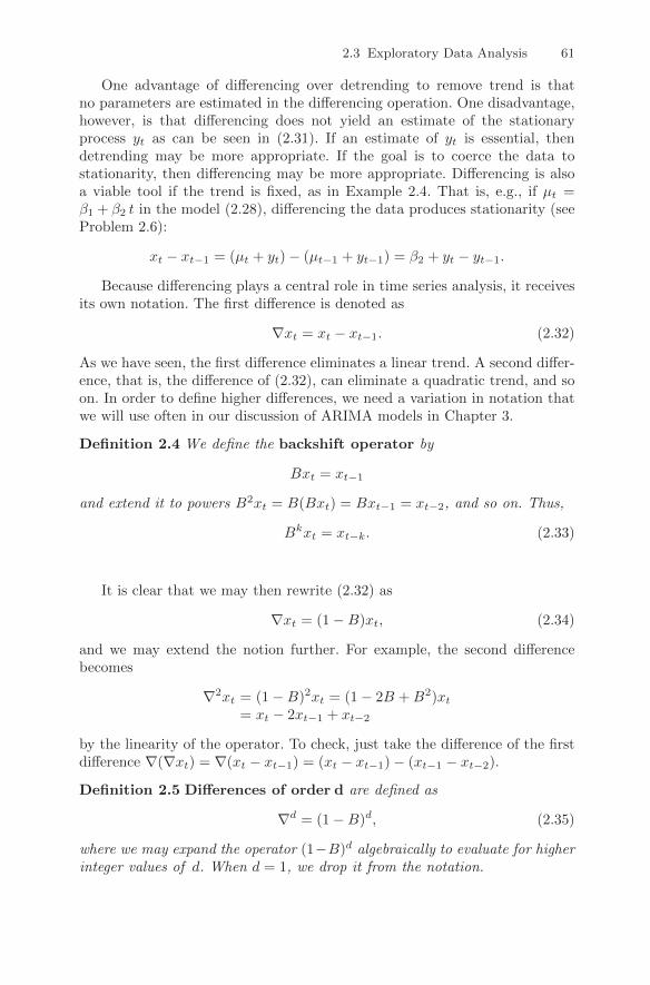
Because differencing plays a central role in time series analysis, it receivesits own notation. The first difference is denoted as

∇xt = xt − xt−1. (2.32)

As we have seen, the first difference eliminates a linear trend. A second differ-ence, that is, the difference of (2.32), can eliminate a quadratic trend, and soon. In order to define higher differences, we need a variation in notation thatwe will use often in our discussion of ARIMA models in Chapter 3.

Definition 2.4 We define the backshift operator by

Bxt = xt−1

and extend it to powers B2xt = B(Bxt) = Bxt−1 = xt−2, and so on. Thus,

Bkxt = xt−k. (2.33)

It is clear that we may then rewrite (2.32) as

∇xt = (1−B)xt, (2.34)

and we may extend the notion further. For example, the second differencebecomes

∇2xt = (1−B)2xt = (1− 2B +B2)xt= xt − 2xt−1 + xt−2

by the linearity of the operator. To check, just take the difference of the firstdifference ∇(∇xt) = ∇(xt − xt−1) = (xt − xt−1)− (xt−1 − xt−2).

Definition 2.5 Differences of order d are defined as

∇d = (1−B)d, (2.35)

where we may expand the operator (1−B)d algebraically to evaluate for higherinteger values of d. When d = 1, we drop it from the notation.


The first difference (2.32) is an example of a linear filter applied to elim-inate a trend. Other filters, formed by averaging values near xt, can pro-duce adjusted series that eliminate other kinds of unwanted fluctuations, asin Chapter 3. The differencing technique is an important component of theARIMA model of Box and Jenkins (1970) (see also Box et al., 1994), to bediscussed in Chapter 3.

Example 2.5 Differencing Global Temperature

The first difference of the global temperature series, also shown in Figure 2.4,produces different results than removing trend by detrending via regression.For example, the differenced series does not contain the long middle cyclewe observe in the detrended series. The ACF of this series is also shown inFigure 2.5. In this case it appears that the differenced process shows minimalautocorrelation, which may imply the global temperature series is nearly arandom walk with drift. It is interesting to note that if the series is a randomwalk with drift, the mean of the differenced series, which is an estimate ofthe drift, is about .0066 (but with a large standard error):

1 mean(diff(gtemp)) # = 0.00659 (drift)

2 sd(diff(gtemp))/sqrt(length(diff(gtemp))) # = 0.00966 (SE)

An alternative to differencing is a less-severe operation that still assumesstationarity of the underlying time series. This alternative, called fractionaldifferencing, extends the notion of the difference operator (2.35) to fractionalpowers −.5 < d < .5, which still define stationary processes. Granger andJoyeux (1980) and Hosking (1981) introduced long memory time series, whichcorresponds to the case when 0 < d < .5. This model is often used for en-vironmental time series arising in hydrology. We will discuss long memoryprocesses in more detail in §5.2.

Often, obvious aberrations are present that can contribute nonstationaryas well as nonlinear behavior in observed time series. In such cases, transfor-mations may be useful to equalize the variability over the length of a singleseries. A particularly useful transformation is

yt = log xt, (2.36)

which tends to suppress larger fluctuations that occur over portions of theseries where the underlying values are larger. Other possibilities are powertransformations in the Box–Cox family of the form

yt =

{(xλt − 1)/λ λ 6= 0,

log xt λ = 0.(2.37)

Methods for choosing the power λ are available (see Johnson and Wichern,1992, §4.7) but we do not pursue them here. Often, transformations are alsoused to improve the approximation to normality or to improve linearity inpredicting the value of one series from another.


varve

0 100 200 300 400 500 600

050

100

150

log(varve)

0 100 200 300 400 500 600

23

45

Fig. 2.6. Glacial varve thicknesses (top) from Massachusetts for n = 634 yearscompared with log transformed thicknesses (bottom).

Example 2.6 Paleoclimatic Glacial Varves

Melting glaciers deposit yearly layers of sand and silt during the springmelting seasons, which can be reconstructed yearly over a period rangingfrom the time deglaciation began in New England (about 12,600 years ago)to the time it ended (about 6,000 years ago). Such sedimentary deposits,called varves, can be used as proxies for paleoclimatic parameters, such astemperature, because, in a warm year, more sand and silt are depositedfrom the receding glacier. Figure 2.6 shows the thicknesses of the yearlyvarves collected from one location in Massachusetts for 634 years, beginning11,834 years ago. For further information, see Shumway and Verosub (1992).Because the variation in thicknesses increases in proportion to the amountdeposited, a logarithmic transformation could remove the nonstationarityobservable in the variance as a function of time. Figure 2.6 shows the originaland transformed varves, and it is clear that this improvement has occurred.We may also plot the histogram of the original and transformed data, asin Problem 2.8, to argue that the approximation to normality is improved.The ordinary first differences (2.34) are also computed in Problem 2.8, andwe note that the first differences have a significant negative correlation at


lag h = 1. Later, in Chapter 5, we will show that perhaps the varve serieshas long memory and will propose using fractional differencing.

Figure 2.6 was generated in R as follows:1 par(mfrow=c(2,1))

2 plot(varve, main="varve", ylab="")

3 plot(log(varve), main="log(varve)", ylab="" )

Next, we consider another preliminary data processing technique that isused for the purpose of visualizing the relations between series at different lags,namely, scatterplot matrices. In the definition of the ACF, we are essentiallyinterested in relations between xt and xt−h; the autocorrelation function tellsus whether a substantial linear relation exists between the series and its ownlagged values. The ACF gives a profile of the linear correlation at all possiblelags and shows which values of h lead to the best predictability. The restrictionof this idea to linear predictability, however, may mask a possible nonlinearrelation between current values, xt, and past values, xt−h. This idea extendsto two series where one may be interested in examining scatterplots of ytversus xt−h

Example 2.7 Scatterplot Matrices, SOI and Recruitment

To check for nonlinear relations of this form, it is convenient to display alagged scatterplot matrix, as in Figure 2.7, that displays values of the SOI,St, on the vertical axis plotted against St−h on the horizontal axis. Thesample autocorrelations are displayed in the upper right-hand corner andsuperimposed on the scatterplots are locally weighted scatterplot smoothing(lowess) lines that can be used to help discover any nonlinearities. We discusssmoothing in the next section, but for now, think of lowess as a robustmethod for fitting nonlinear regression.

In Figure 2.7, we notice that the lowess fits are approximately linear,so that the sample autocorrelations are meaningful. Also, we see strongpositive linear relations at lags h = 1, 2, 11, 12, that is, between St andSt−1, St−2, St−11, St−12, and a negative linear relation at lags h = 6, 7. Theseresults match up well with peaks noticed in the ACF in Figure 1.14.

Similarly, we might want to look at values of one series, say Recruitment,denoted Rt plotted against another series at various lags, say the SOI, St−h,to look for possible nonlinear relations between the two series. Because,for example, we might wish to predict the Recruitment series, Rt, fromcurrent or past values of the SOI series, St−h, for h = 0, 1, 2, ... it would beworthwhile to examine the scatterplot matrix. Figure 2.8 shows the laggedscatterplot of the Recruitment series Rt on the vertical axis plotted againstthe SOI index St−h on the horizontal axis. In addition, the figure exhibitsthe sample cross-correlations as well as lowess fits.

Figure 2.8 shows a fairly strong nonlinear relationship between Recruit-ment, Rt, and the SOI series at St−5, St−6, St−7, St−8, indicating the SOIseries tends to lead the Recruitment series and the coefficients are negative,implying that increases in the SOI lead to decreases in the Recruitment. The


−1.0 −0.5 0.0 0.5 1.0

−1.

00.

00.

51.

0soi(t−1)

soi(t

)

0.6

−1.0 −0.5 0.0 0.5 1.0

−1.

00.

00.

51.

0

soi(t−2)

soi(t

)

0.37

−1.0 −0.5 0.0 0.5 1.0

−1.

00.

00.

51.

0

soi(t−3)

soi(t

)

0.21

−1.0 −0.5 0.0 0.5 1.0

−1.

00.

00.

51.

0

soi(t−4)

soi(t

)

0.05

−1.0 −0.5 0.0 0.5 1.0

−1.

00.

00.

51.

0

soi(t−5)

soi(t

)−0.11

−1.0 −0.5 0.0 0.5 1.0

−1.

00.

00.

51.

0

soi(t−6)

soi(t

)

−0.19

−1.0 −0.5 0.0 0.5 1.0

−1.

00.

00.

51.

0

soi(t−7)

soi(t

)

−0.18

−1.0 −0.5 0.0 0.5 1.0

−1.

00.

00.

51.

0

soi(t−8)

soi(t

)

−0.1

−1.0 −0.5 0.0 0.5 1.0−

1.0

0.0

0.5

1.0

soi(t−9)

soi(t

)

0.05

−1.0 −0.5 0.0 0.5 1.0

−1.

00.

00.

51.

0

soi(t−10)

soi(t

)

0.22

−1.0 −0.5 0.0 0.5 1.0

−1.

00.

00.

51.

0

soi(t−11)

soi(t

)

0.36

−1.0 −0.5 0.0 0.5 1.0

−1.

00.

00.

51.

0

soi(t−12)

soi(t

)

0.41

Fig. 2.7. Scatterplot matrix relating current SOI values, St, to past SOI values,St−h, at lags h = 1, 2, ..., 12. The values in the upper right corner are the sampleautocorrelations and the lines are a lowess fit.

nonlinearity observed in the scatterplots (with the help of the superimposedlowess fits) indicate that the behavior between Recruitment and the SOI isdifferent for positive values of SOI than for negative values of SOI.

Simple scatterplot matrices for one series can be obtained in R usingthe lag.plot command. Figures 2.7 and 2.8 may be reproduced using thefollowing scripts provided with the text (see Appendix R for detials):

1 lag.plot1(soi, 12) # Fig 2.7

2 lag.plot2(soi, rec, 8) # Fig 2.8

As a final exploratory tool, we discuss assessing periodic behavior in timeseries data using regression analysis and the periodogram; this material maybe thought of as an introduction to spectral analysis, which we discuss in


−1.0 −0.5 0.0 0.5 1.0

020

4060

8010

0soi(t−0)

rec(

t)

0.02

−1.0 −0.5 0.0 0.5 1.0

020

4060

8010

0

soi(t−1)

rec(

t)

0.01

−1.0 −0.5 0.0 0.5 1.0

020

4060

8010

0

soi(t−2)

rec(

t)

−0.04

−1.0 −0.5 0.0 0.5 1.0

020

4060

8010

0

soi(t−3)

rec(

t)

−0.15

−1.0 −0.5 0.0 0.5 1.0

020

4060

8010

0soi(t−4)

rec(

t)

−0.3

−1.0 −0.5 0.0 0.5 1.0

020

4060

8010

0

soi(t−5)

rec(

t)

−0.53

−1.0 −0.5 0.0 0.5 1.0

020

4060

8010

0

soi(t−6)

rec(

t)

−0.6

−1.0 −0.5 0.0 0.5 1.0

020

4060

8010

0

soi(t−7)

rec(

t)

−0.6

−1.0 −0.5 0.0 0.5 1.0

020

4060

8010

0soi(t−8)re

c(t)

−0.56

Fig. 2.8. Scatterplot matrix of the Recruitment series, Rt, on the vertical axisplotted against the SOI series, St−h, on the horizontal axis at lags h = 0, 1, . . . , 8.The values in the upper right corner are the sample cross-correlations and the linesare a lowess fit.

detail in Chapter 4. In Example 1.12, we briefly discussed the problem ofidentifying cyclic or periodic signals in time series. A number of the timeseries we have seen so far exhibit periodic behavior. For example, the datafrom the pollution study example shown in Figure 2.2 exhibit strong yearlycycles. Also, the Johnson & Johnson data shown in Figure 1.1 make one cycleevery year (four quarters) on top of an increasing trend and the speech datain Figure 1.2 is highly repetitive. The monthly SOI and Recruitment series inFigure 1.6 show strong yearly cycles, but hidden in the series are clues to theEl Nino cycle.


Example 2.8 Using Regression to Discover a Signal in Noise

In Example 1.12, we generated n = 500 observations from the model

xt = A cos(2πωt+ φ) + wt, (2.38)

where ω = 1/50, A = 2, φ = .6π, and σw = 5; the data are shown onthe bottom panel of Figure 1.11 on page 16. At this point we assume thefrequency of oscillation ω = 1/50 is known, but A and φ are unknownparameters. In this case the parameters appear in (2.38) in a nonlinear way,so we use a trigonometric identity4 and write

A cos(2πωt+ φ) = β1 cos(2πωt) + β2 sin(2πωt),

where β1 = A cos(φ) and β2 = −A sin(φ). Now the model (2.38) can bewritten in the usual linear regression form given by (no intercept term isneeded here)

xt = β1 cos(2πt/50) + β2 sin(2πt/50) + wt. (2.39)

Using linear regression on the generated data, the fitted model is

xt = −.71(.30) cos(2πt/50)− 2.55(.30) sin(2πt/50) (2.40)

with σw = 4.68, where the values in parentheses are the standard er-rors. We note the actual values of the coefficients for this example areβ1 = 2 cos(.6π) = −.62 and β2 = −2 sin(.6π) = −1.90. Because the pa-rameter estimates are significant and close to the actual values, it is clearthat we are able to detect the signal in the noise using regression, eventhough the signal appears to be obscured by the noise in the bottom panelof Figure 1.11. Figure 2.9 shows data generated by (2.38) with the fittedline, (2.40), superimposed.

To reproduce the analysis and Figure 2.9 in R, use the following com-mands:

1 set.seed(1000) # so you can reproduce these results

2 x = 2*cos(2*pi*1:500/50 + .6*pi) + rnorm(500,0,5)

3 z1 = cos(2*pi*1:500/50); z2 = sin(2*pi*1:500/50)

4 summary(fit <- lm(x~0+z1+z2)) # zero to exclude the intercept

5 plot.ts(x, lty="dashed")

6 lines(fitted(fit), lwd=2)

Example 2.9 Using the Periodogram to Discover a Signal in Noise

The analysis in Example 2.8 may seem like cheating because we assumed weknew the value of the frequency parameter ω. If we do not know ω, we couldtry to fit the model (2.38) using nonlinear regression with ω as a parameter.Another method is to try various values of ω in a systematic way. Using the

4 cos(α± β) = cos(α) cos(β)∓ sin(α) sin(β).


Time

x

0 100 200 300 400 500

−15

−10

−50

510

Fig. 2.9. Data generated by (2.38) [dashed line] with the fitted [solid] line, (2.40),superimposed.

regression results of §2.2, we can show the estimated regression coefficientsin Example 2.8 take on the special form given by

β1 =

∑nt=1 xt cos(2πt/50)∑nt=1 cos2(2πt/50)

=2

n

n∑t=1

xt cos(2πt/50); (2.41)

β2 =

∑nt=1 xt sin(2πt/50)∑nt=1 sin2(2πt/50)

=2

n

n∑t=1

xt sin(2πt/50). (2.42)

This suggests looking at all possible regression parameter estimates,5 say

β1(j/n) =2

n

n∑t=1

xt cos(2πt j/n); (2.43)

β2(j/n) =2

n

n∑t=1

xt sin(2πt j/n), (2.44)

where, n = 500 and j = 1, . . . , n2 − 1, and inspecting the results for large

values. For the endpoints, j = 0 and j = n/2, we have β1(0) = n−1∑nt=1 xt

and β1( 12 ) = n−1

∑nt=1(−1)txt, and β2(0) = β2( 1

2 ) = 0.For this particular example, the values calculated in (2.41) and (2.42) are

β1(10/500) and β2(10/500). By doing this, we have regressed a series, xt, of

5 In the notation of §2.2, the estimates are of the form∑nt=1 xtzt

/ ∑nt=1 z

2t where

zt = cos(2πtj/n) or zt = sin(2πtj/n). In this setup, unless j = 0 or j = n/2 if nis even,

∑nt=1 z

2t = n/2; see Problem 2.10.


0.0 0.1 0.2 0.3 0.4 0.5

01

23

45

67

Frequency

Sca

led

Perio

dogr

am

Fig. 2.10. The scaled periodogram, (2.45), of the 500 observations generated by(2.38); the data are displayed in Figures 1.11 and 2.9.

length n using n regression parameters, so that we will have a perfect fit.The point, however, is that if the data contain any cyclic behavior we arelikely to catch it by performing these saturated regressions.

Next, note that the regression coefficients β1(j/n) and β2(j/n), for eachj, are essentially measuring the correlation of the data with a sinusoid os-cillating at j cycles in n time points.6 Hence, an appropriate measure of thepresence of a frequency of oscillation of j cycles in n time points in the datawould be

P (j/n) = β21(j/n) + β2

2(j/n), (2.45)

which is basically a measure of squared correlation. The quantity (2.45)is sometimes called the periodogram, but we will call P (j/n) the scaledperiodogram and we will investigate its properties in Chapter 4. Figure 2.10shows the scaled periodogram for the data generated by (2.38), and it easilydiscovers the periodic component with frequency ω = .02 = 10/500 eventhough it is difficult to visually notice that component in Figure 1.11 dueto the noise.

Finally, we mention that it is not necessary to run a large regression

xt =

n/2∑j=0

β1(j/n) cos(2πtj/n) + β2(j/n) sin(2πtj/n) (2.46)

to obtain the values of β1(j/n) and β2(j/n) [with β2(0) = β2(1/2) = 0]because they can be computed quickly if n (assumed even here) is a highly

6 Sample correlations are of the form∑t xtzt

/ (∑t x

2t

∑t z

2t

)1/2.


composite integer. There is no error in (2.46) because there are n obser-vations and n parameters; the regression fit will be perfect. The discreteFourier transform (DFT) is a complex-valued weighted average of the datagiven by

d(j/n) = n−1/2n∑t=1

xt exp(−2πitj/n)

= n−1/2

(n∑t=1

xt cos(2πtj/n)− in∑t=1

xt sin(2πtj/n)

) (2.47)

where the frequencies j/n are called the Fourier or fundamental frequencies.Because of a large number of redundancies in the calculation, (2.47) may becomputed quickly using the fast Fourier transform (FFT)7, which is availablein many computing packages such as Matlab R©, S-PLUS R© and R. Note that8

|d(j/n)|2 =1

n

(n∑t=1

xt cos(2πtj/n)

)2

+1

n

(n∑t=1

xt sin(2πtj/n)

)2

(2.48)

and it is this quantity that is called the periodogram; we will write

I(j/n) = |d(j/n)|2.

We may calculate the scaled periodogram, (2.45), using the periodogram as

P (j/n) =4

nI(j/n). (2.49)

We will discuss this approach in more detail and provide examples with datain Chapter 4.

Figure 2.10 can be created in R using the following commands (and thedata already generated in x):

1 I = abs(fft(x))^2/500 # the periodogram

2 P = (4/500)*I[1:250] # the scaled periodogram

3 f = 0:249/500 # frequencies

4 plot(f, P, type="l", xlab="Frequency", ylab="Scaled Periodogram")

2.4 Smoothing in the Time Series Context

In §1.4, we introduced the concept of smoothing a time series, and in Ex-ample 1.9, we discussed using a moving average to smooth white noise. Thismethod is useful in discovering certain traits in a time series, such as long-term

7 Different packages scale the FFT differently; consult the documentation. R cal-culates (2.47) without scaling by n−1/2.

8 If z = a− ib is complex, then |z|2 = zz = (a− ib)(a+ ib) = a2 + b2.

2.4 Smoothing in the Time Series Context 71

Fig. 2.11. The weekly cardiovascular mortality series discussed in Example 2.2smoothed using a five-week moving average and a 53-week moving average.

trend and seasonal components. In particular, if xt represents the observations,then

mt =k∑

j=−k

ajxt−j , (2.50)

where aj = a−j ≥ 0 and∑kj=−k aj = 1 is a symmetric moving average of the

data.

Example 2.10 Moving Average Smoother

For example, Figure 2.11 shows the weekly mortality series discussed inExample 2.2, a five-point moving average (which is essentially a monthlyaverage with k = 2) that helps bring out the seasonal component and a53-point moving average (which is essentially a yearly average with k = 26)that helps bring out the (negative) trend in cardiovascular mortality. In bothcases, the weights, a−k, . . . , a0, . . . , ak, we used were all the same, and equalto 1/(2k + 1).9

To reproduce Figure 2.11 in R:1 ma5 = filter(cmort, sides=2, rep(1,5)/5)

2 ma53 = filter(cmort, sides=2, rep(1,53)/53)

3 plot(cmort, type="p", ylab="mortality")

4 lines(ma5); lines(ma53)

9 Sometimes, the end weights, a−k and ak are set equal to half the value of theother weights.


Fig. 2.12. The weekly cardiovascular mortality series with a cubic trend and cubictrend plus periodic regression.

Many other techniques are available for smoothing time series data basedon methods from scatterplot smoothers. The general setup for a time plot is

xt = ft + yt, (2.51)

where ft is some smooth function of time, and yt is a stationary process. Wemay think of the moving average smoother mt, given in (2.50), as an estimatorof ft. An obvious choice for ft in (2.51) is polynomial regression

ft = β0 + β1t+ · · ·+ βptp. (2.52)

We have seen the results of a linear fit on the global temperature data inExample 2.1. For periodic data, one might employ periodic regression

ft = α0 + α1 cos(2πω1t) + β1 sin(2πω1t)

+ · · ·+ αp cos(2πωpt) + βp sin(2πωpt), (2.53)

where ω1, . . . , ωp are distinct, specified frequencies. In addition, one mightconsider combining (2.52) and (2.53). These smoothers can be applied usingclassical linear regression.

Example 2.11 Polynomial and Periodic Regression Smoothers

Figure 2.12 shows the weekly mortality series with an estimated (via ordi-nary least squares) cubic smoother

ft = β0 + β1t+ β2t2 + β3t

3


superimposed to emphasize the trend, and an estimated (via ordinary leastsquares) cubic smoother plus a periodic regression

ft = β0 + β1t+ β2t2 + β3t

3 + α1 cos(2πt/52) + α2 sin(2πt/52)

superimposed to emphasize trend and seasonality.The R commands for this example are as follows (we note that the sam-

pling rate is 1/52, so that wk below is essentially t/52).1 wk = time(cmort) - mean(time(cmort))

2 wk2 = wk^2; wk3 = wk^3

3 cs = cos(2*pi*wk); sn = sin(2*pi*wk)

4 reg1 = lm(cmort~wk + wk2 + wk3, na.action=NULL)

5 reg2 = lm(cmort~wk + wk2 + wk3 + cs + sn, na.action=NULL)


7 lines(fitted(reg1)); lines(fitted(reg2))

Modern regression techniques can be used to fit general smoothers to thepairs of points (t, xt) where the estimate of ft is smooth. Many of the tech-niques can easily be applied to time series data using the R or S-PLUS sta-tistical packages; see Venables and Ripley (1994, Chapter 10) for details onapplying these methods in S-PLUS (R is similar). A problem with the tech-niques used in Example 2.11 is that they assume ft is the same function overthe range of time, t; we might say that the technique is global. The movingaverage smoothers in Example 2.10 fit the data better because the techniqueis local; that is, moving average smoothers allow for the possibility that ft isa different function over time. We describe some other local methods in thefollowing examples.

Example 2.12 Kernel Smoothing

Kernel smoothing is a moving average smoother that uses a weight function,or kernel, to average the observations. Figure 2.13 shows kernel smoothingof the mortality series, where ft in (2.51) is estimated by

ft =n∑i=1

wi(t)xi, (2.54)

where

wi(t) = K(t−ib

) / n∑j=1

K(t−jb

). (2.55)

are the weights and K(·) is a kernel function. This estimator, which wasoriginally explored by Parzen (1962) and Rosenblatt (1956b), is often calledthe Nadaraya–Watson estimator (Watson, 1966); typically, the normal ker-nel, K(z) = 1√

2πexp(−z2/2), is used. To implement this in R, use the

ksmooth function. The wider the bandwidth, b, the smoother the result.In Figure 2.13, the values of b for this example were b = 5/52 (roughly


Fig. 2.13. Kernel smoothers of the mortality data.

weighted two to three week averages because b/2 is the inner quartile rangeof the kernel) for the seasonal component, and b = 104/52 = 2 (roughlyweighted yearly averages) for the trend component.

Figure 2.13 can be reproduced in R (or S-PLUS) as follows.1 plot(cmort, type="p", ylab="mortality")

2 lines(ksmooth(time(cmort), cmort, "normal", bandwidth=5/52))

3 lines(ksmooth(time(cmort), cmort, "normal", bandwidth=2))

Example 2.13 Lowess and Nearest Neighbor Regression

Another approach to smoothing a time plot is nearest neighbor regression.The technique is based on k-nearest neighbors linear regression, wherein oneuses the data {xt−k/2, . . . , xt, . . . , xt+k/2} to predict xt using linear regres-

sion; the result is ft. For example, Figure 2.14 shows cardiovascular mor-tality and the nearest neighbor method using the R (or S-PLUS) smoothersupsmu. We used k = n/2 to estimate the trend and k = n/100 to esti-mate the seasonal component. In general, supsmu uses a variable windowfor smoothing (see Friedman, 1984), but it can be used for correlated databy fixing the smoothing window, as was done here.

Lowess is a method of smoothing that is rather complex, but the basic ideais close to nearest neighbor regression. Figure 2.14 shows smoothing of mor-tality using the R or S-PLUS function lowess (see Cleveland, 1979). First,a certain proportion of nearest neighbors to xt are included in a weightingscheme; values closer to xt in time get more weight. Then, a robust weightedregression is used to predict xt and obtain the smoothed estimate of ft. Thelarger the fraction of nearest neighbors included, the smoother the estimate


nearest neighborm

orta

lity

1970 1972 1974 1976 1978 1980

7080

9011

013

0

lowess

mor

talit

y

1970 1972 1974 1976 1978 1980

7080

9011

013

0

Fig. 2.14. Nearest neighbor (supsmu) and locally weighted regression (lowess)smoothers of the mortality data.

ft will be. In Figure 2.14, the smoother uses about two-thirds of the datato obtain an estimate of the trend component, and the seasonal componentuses 2% of the data.

Figure 2.14 can be reproduced in R or S-PLUS as follows.1 par(mfrow=c(2,1))

2 plot(cmort, type="p", ylab="mortality", main="nearest neighbor")

3 lines(supsmu(time(cmort), cmort, span=.5))

4 lines(supsmu(time(cmort), cmort, span=.01))

5 plot(cmort, type="p", ylab="mortality", main="lowess")

6 lines(lowess(cmort, f=.02)); lines(lowess(cmort, f=2/3))

Example 2.14 Smoothing Splines

An extension of polynomial regression is to first divide time t = 1, . . . , n,into k intervals, [t0 = 1, t1], [t1 + 1, t2] , . . . , [tk−1 + 1, tk = n]. The valuest0, t1, . . . , tk are called knots. Then, in each interval, one fits a regression ofthe form (2.52); typically, p = 3, and this is called cubic splines.

A related method is smoothing splines, which minimizes a compromisebetween the fit and the degree of smoothness given by


Fig. 2.15. Smoothing splines fit to the mortality data.

n∑t=1

[xt − ft]2 + λ

∫ (f′′

t

)2dt, (2.56)

where ft is a cubic spline with a knot at each t. The degree of smoothness iscontrolled by λ > 0. There is a relationship between smoothing splines andstate space models, which is investigated in Problem 6.7.

In R, the smoothing parameter is called spar and it is monotonicallyrelated to λ; type ?smooth.spline to view the help file for details. Fig-ure 2.15 shows smoothing spline fits on the mortality data using generalizedcross-validation, which uses the data to “optimally” assess the smoothingparameter, for the seasonal component, and spar=1 for the trend. The figurecan be reproduced in R as follows.


2 lines(smooth.spline(time(cmort), cmort))

3 lines(smooth.spline(time(cmort), cmort, spar=1))

Example 2.15 Smoothing One Series as a Function of Another

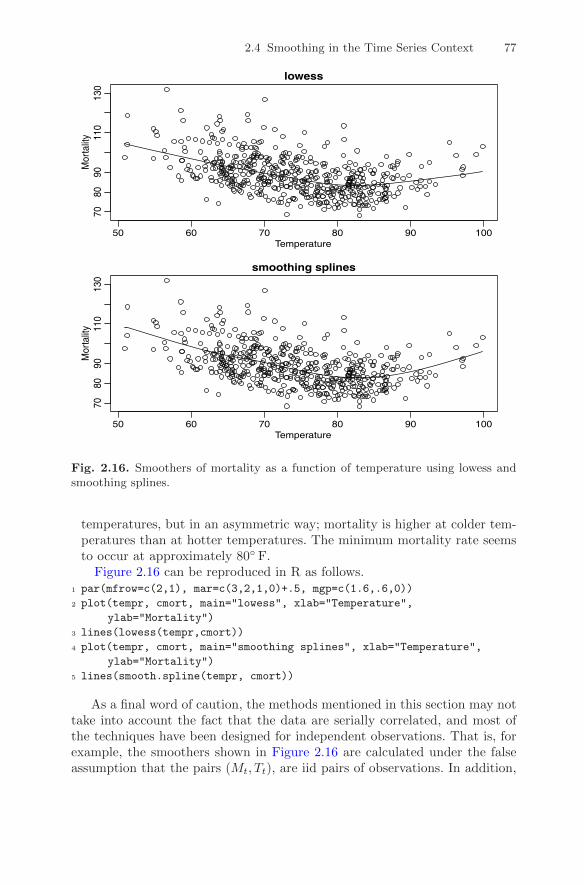
In addition to smoothing time plots, smoothing techniques can be appliedto smoothing a time series as a function of another time series. In this ex-ample, we smooth the scatterplot of two contemporaneously measured timeseries, mortality as a function of temperature. In Example 2.2, we discov-ered a nonlinear relationship between mortality and temperature. Continu-ing along these lines, Figure 2.16 shows scatterplots of mortality, Mt, andtemperature, Tt, along with Mt smoothed as a function of Tt using lowessand using smoothing splines. In both cases, mortality increases at extreme


50 60 70 80 90 100

7080

9011

013

0

lowess

Temperature

Mor

talit

y

50 60 70 80 90 100

7080

9011

013

0

smoothing splines

Temperature

Mor

talit

y

Fig. 2.16. Smoothers of mortality as a function of temperature using lowess andsmoothing splines.

temperatures, but in an asymmetric way; mortality is higher at colder tem-peratures than at hotter temperatures. The minimum mortality rate seemsto occur at approximately 80◦ F.

Figure 2.16 can be reproduced in R as follows.1 par(mfrow=c(2,1), mar=c(3,2,1,0)+.5, mgp=c(1.6,.6,0))

2 plot(tempr, cmort, main="lowess", xlab="Temperature",

ylab="Mortality")

3 lines(lowess(tempr,cmort))

4 plot(tempr, cmort, main="smoothing splines", xlab="Temperature",

ylab="Mortality")

5 lines(smooth.spline(tempr, cmort))

As a final word of caution, the methods mentioned in this section may nottake into account the fact that the data are serially correlated, and most ofthe techniques have been designed for independent observations. That is, forexample, the smoothers shown in Figure 2.16 are calculated under the falseassumption that the pairs (Mt, Tt), are iid pairs of observations. In addition,


the degree of smoothness used in the previous examples were chosen arbitrarilyto bring out what might be considered obvious features in the data set.

Problems

Section 2.2

2.1 For the Johnson & Johnson data, say yt, shown in Figure 1.1, let xt =log(yt).

(a) Fit the regression model

xt = βt+ α1Q1(t) + α2Q2(t) + α3Q3(t) + α4Q4(t) + wt

where Qi(t) = 1 if time t corresponds to quarter i = 1, 2, 3, 4, and zerootherwise. The Qi(t)’s are called indicator variables. We will assume fornow that wt is a Gaussian white noise sequence. What is the interpreta-tion of the parameters β, α1, α2, α3, and α4? (Detailed code is given inAppendix R on page 574.)

(b) What happens if you include an intercept term in the model in (a)?(c) Graph the data, xt, and superimpose the fitted values, say xt, on the

graph. Examine the residuals, xt− xt, and state your conclusions. Does itappear that the model fits the data well (do the residuals look white)?

2.2 For the mortality data examined in Example 2.2:

(a) Add another component to the regression in (2.25) that accounts for theparticulate count four weeks prior; that is, add Pt−4 to the regression in(2.25). State your conclusion.

(b) Draw a scatterplot matrix of Mt, Tt, Pt and Pt−4 and then calculate thepairwise correlations between the series. Compare the relationship betweenMt and Pt versus Mt and Pt−4.

2.3 Repeat the following exercise six times and then discuss the results. Gen-erate a random walk with drift, (1.4), of length n = 100 with δ = .01 andσw = 1. Call the data xt for t = 1, . . . , 100. Fit the regression xt = βt + wtusing least squares. Plot the data, the mean function (i.e., µt = .01 t) and the

fitted line, xt = β t, on the same graph. Discuss your results.

The following R code may be useful:

1 par(mfcol = c(3,2)) # set up graphics

2 for (i in 1:6){

3 x = ts(cumsum(rnorm(100,.01,1))) # the data

4 reg = lm(x~0+time(x), na.action=NULL) # the regression

5 plot(x) # plot data

6 lines(.01*time(x), col="red", lty="dashed") # plot mean

7 abline(reg, col="blue") } # plot regression line

Problems 79

2.4 Kullback-Leibler Information. Given the random vector yyy, we define theinformation for discriminating between two densities in the same family, in-dexed by a parameter θθθ, say f(yyy; θθθ1) and f(yyy; θθθ2), as

I(θθθ1; θθθ2) =1

nE1 log

f(yyy; θθθ1)

f(yyy; θθθ2), (2.57)

where E1 denotes expectation with respect to the density determined by θθθ1.For the Gaussian regression model, the parameters are θθθ = (βββ′, σ2)′. Showthat we obtain

I(θθθ1; θθθ2) =1

2

(σ21

σ22

− logσ21

σ22

− 1

)+

1

2

(βββ1 − βββ2)′Z ′Z(βββ1 − βββ2)

nσ22

(2.58)

in that case.

2.5 Model Selection. Both selection criteria (2.19) and (2.20) are derived frominformation theoretic arguments, based on the well-known Kullback-Leiblerdiscrimination information numbers (see Kullback and Leibler, 1951, Kull-back, 1958). We give an argument due to Hurvich and Tsai (1989). We thinkof the measure (2.58) as measuring the discrepancy between the two densities,characterized by the parameter values θθθ′1 = (βββ′1, σ

21)′ and θθθ′2 = (βββ′2, σ

22)′. Now,

if the true value of the parameter vector is θθθ1, we argue that the best modelwould be one that minimizes the discrepancy between the theoretical valueand the sample, say I(θθθ1; θθθ). Because θθθ1 will not be known, Hurvich and Tsai

(1989) considered finding an unbiased estimator for E1[I(βββ1, σ21 ; βββ,σ

2)], where

I(βββ1, σ21 ; βββ,σ

2) =1

2

(σ21

σ2− log

σ21

σ2− 1

)+

1

2

(βββ1 − βββ)′Z ′Z(βββ1 − βββ)

nσ2

and βββ is a k × 1 regression vector. Show that

E1[I(βββ1, σ21 ; βββ,σ

2)] =1

2

(− log σ2

1 + E1 log σ2 +n+ k

n− k − 2− 1

), (2.59)

using the distributional properties of the regression coefficients and error vari-ance. An unbiased estimator for E1 log σ2 is log σ2. Hence, we have shownthat the expectation of the above discrimination information is as claimed.As models with differing dimensions k are considered, only the second andthird terms in (2.59) will vary and we only need unbiased estimators for thosetwo terms. This gives the form of AICc quoted in (2.20) in the chapter. Youwill need the two distributional results

nσ2

σ21

∼ χ2n−k and

(βββ − βββ1)′Z ′Z(βββ − βββ1)

σ21

∼ χ2k

The two quantities are distributed independently as chi-squared distributionswith the indicated degrees of freedom. If x ∼ χ2

n, E(1/x) = 1/(n− 2).


Section 2.3

2.6 Consider a process consisting of a linear trend with an additive noise termconsisting of independent random variables wt with zero means and variancesσ2w, that is,

xt = β0 + β1t+ wt,

where β0, β1 are fixed constants.

(a) Prove xt is nonstationary.(b) Prove that the first difference series ∇xt = xt − xt−1 is stationary by

finding its mean and autocovariance function.(c) Repeat part (b) if wt is replaced by a general stationary process, say yt,

with mean function µy and autocovariance function γy(h).

2.7 Show (2.31) is stationary.

2.8 The glacial varve record plotted in Figure 2.6 exhibits some nonstationar-ity that can be improved by transforming to logarithms and some additionalnonstationarity that can be corrected by differencing the logarithms.

(a) Argue that the glacial varves series, say xt, exhibits heteroscedasticity bycomputing the sample variance over the first half and the second half ofthe data. Argue that the transformation yt = log xt stabilizes the vari-ance over the series. Plot the histograms of xt and yt to see whether theapproximation to normality is improved by transforming the data.

(b) Plot the series yt. Do any time intervals, of the order 100 years, existwhere one can observe behavior comparable to that observed in the globaltemperature records in Figure 1.2?

(c) Examine the sample ACF of yt and comment.(d) Compute the difference ut = yt − yt−1, examine its time plot and sample

ACF, and argue that differencing the logged varve data produces a rea-sonably stationary series. Can you think of a practical interpretation forut? Hint: For |p| close to zero, log(1 + p) ≈ p; let p = (yt − yt−1)/yt−1.

(e) Based on the sample ACF of the differenced transformed series computedin (c), argue that a generalization of the model given by Example 1.23might be reasonable. Assume

ut = µ+ wt − θwt−1

is stationary when the inputs wt are assumed independent with mean 0and variance σ2

w. Show that

γu(h) =

σ2w(1 + θ2) if h = 0,

−θ σ2w if h = ±1,

0 if |h| > 1.

Problems 81

(f) Based on part (e), use ρu(1) and the estimate of the variance of ut, γu(0),to derive estimates of θ and σ2

w. This is an application of the method ofmoments from classical statistics, where estimators of the parameters arederived by equating sample moments to theoretical moments.

2.9 In this problem, we will explore the periodic nature of St, the SOI seriesdisplayed in Figure 1.5.

(a) Detrend the series by fitting a regression of St on time t. Is there a signif-icant trend in the sea surface temperature? Comment.

(b) Calculate the periodogram for the detrended series obtained in part (a).Identify the frequencies of the two main peaks (with an obvious one at thefrequency of one cycle every 12 months). What is the probable El Ninocycle indicated by the minor peak?

2.10 Consider the model (2.46) used in Example 2.9,

xt =n∑j=0

β1(j/n) cos(2πtj/n) + β2(j/n) sin(2πtj/n).

(a) Display the model design matrix Z [see (2.5)] for n = 4.(b) Show numerically that the columns of Z in part (a) satisfy part (d) and

then display (Z ′Z)−1 for this case.(c) If x1, x2, x3, x4 are four observations, write the estimates of the four betas,

β1(0), β1(1/4), β2(1/4), β1(1/2), in terms of the observations.(d) Verify that for any positive integer n and j, k = 0, 1, . . . , [[n/2]], where [[·]]

denotes the greatest integer function:10

(i) Except for j = 0 or j = n/2,

n∑t=1

cos2(2πtj/n) =

n∑t=1

sin2(2πtj/n) = n/2

.(ii) When j = 0 or j = n/2,

n∑t=1

cos2(2πtj/n) = n but

n∑t=1

sin2(2πtj/n) = 0.

(iii) For j 6= k,

n∑t=1

cos(2πtj/n) cos(2πtk/n) =n∑t=1

sin(2πtj/n) sin(2πtk/n) = 0.

Also, for any j and k,

n∑t=1

cos(2πtj/n) sin(2πtk/n) = 0.

10 Some useful facts: 2 cos(α) = eiα + e−iα, 2i sin(α) = eiα − e−iα, and∑nt=1 z

t =z(1− zn)/(1− z) for z 6= 1.


Section 2.4

2.11 Consider the two weekly time series oil and gas. The oil series is indollars per barrel, while the gas series is in cents per gallon; see Appendix Rfor details.

(a) Plot the data on the same graph. Which of the simulated series displayed in§1.3 do these series most resemble? Do you believe the series are stationary(explain your answer)?

(b) In economics, it is often the percentage change in price (termed growth rateor return), rather than the absolute price change, that is important. Arguethat a transformation of the form yt = ∇ log xt might be applied to thedata, where xt is the oil or gas price series [see the hint in Problem 2.8(d)].

(c) Transform the data as described in part (b), plot the data on the samegraph, look at the sample ACFs of the transformed data, and comment.[Hint: poil = diff(log(oil)) and pgas = diff(log(gas)).]

(d) Plot the CCF of the transformed data and comment The small, but signif-icant values when gas leads oil might be considered as feedback. [Hint:ccf(poil, pgas) will have poil leading for negative lag values.]

(e) Exhibit scatterplots of the oil and gas growth rate series for up to threeweeks of lead time of oil prices; include a nonparametric smoother in eachplot and comment on the results (e.g., Are there outliers? Are the rela-tionships linear?). [Hint: lag.plot2(poil, pgas, 3).]

(f) There have been a number of studies questioning whether gasoline pricesrespond more quickly when oil prices are rising than when oil prices arefalling (“asymmetry”). We will attempt to explore this question here withsimple lagged regression; we will ignore some obvious problems such asoutliers and autocorrelated errors, so this will not be a definitive analysis.Let Gt and Ot denote the gas and oil growth rates.

(i) Fit the regression (and comment on the results)

Gt = α1 + α2It + β1Ot + β2Ot−1 + wt,

where It = 1 if Ot ≥ 0 and 0 otherwise (It is the indicator of nogrowth or positive growth in oil price). Hint:

1 indi = ifelse(poil < 0, 0, 1)

2 mess = ts.intersect(pgas, poil, poilL = lag(poil,-1), indi)

3 summary(fit <- lm(pgas~ poil + poilL + indi, data=mess))

(ii) What is the fitted model when there is negative growth in oil price attime t? What is the fitted model when there is no or positive growthin oil price? Do these results support the asymmetry hypothesis?

(iii) Analyze the residuals from the fit and comment.

2.12 Use two different smoothing techniques described in §2.4 to estimate thetrend in the global temperature series displayed in Figure 1.2. Comment.

http://www.springer.com/978-1-4419-7864-6

2 Time Series Regression and Exploratory Data Analysis

Documents