2-Mode Concepts in Social Network Analysis - Steve …steveborgatti.com/papers/2modeconcepts.pdf · 2-Mode Concepts in Social Network Analysis ... In social network analysis, 2-mode

[Forthcoming in Encyclopedia of Complexity and System Science]

2-Mode Concepts in Social Network Analysis Stephen P. Borgatti

Chellgren Chair and Professor of Management Gatton College of Business and Economics

University of Kentucky Lexington, KY 40506 USA

[email protected]

Glossary 1. Definition of Subject 2. Introduction 3. Basic Concepts 4. 2-Mode Data in Social Network Analysis 5. Unimodal Approaches to 2-Mode Data

5.1. Visualization 5.2. Analysis

6. Bimodal Analysis 6.1. Visualization 6.2. Analysis

7. Conclusion 8. Future Directions References Glossary 2-Mode Matrix. A (2-dimensional) matrix is said to be 2-mode if the rows and columns index different sets of entities (e.g., the rows might correspond to persons while the columns correspond to organizations). In contrast, a matrix is 1-mode if the rows and columns refer to the same set of entities, such as a city-by-city matrix if distances. Blockmodel. A blockmodel is a partitioning of the cells of a matrix into blocks that is induced by the partitioning the rows and columns into classes and sorting the matrix such that rows (and columns) that belong to the same class are next to each other. More specifically, two matrix cells xij and xmp are in the same block if class(i) = class(m) and class(j) = class(p). Centrality. A family of concepts of characterizing the structural importance of a node’s position in a network. Graph Cohesion. A family of concepts characterizing the extent of connectedness of a graph, such as density (the proportion of pairs of nodes that have ties), or average path distance.


Multidimensional Scaling (MDS). A method of locating points in space such that Euclidean distances between the points correspond to a matrix of input similarities/distances. Used to provide visual representations of 1-mode matrices such as correlation matrices or perceptual distances among objects. Regular Equivalence. The definition of regular equivalence is recursive. If two nodes are regularly equivalent, then they are connected to regularly equivalent nodes. Regular equivalence is used to identify nodes that are playing the same structural role, even if they are not connected to each other. Social Network (or, in mathematics, a Graph). A collection of nodes (also referred to as vertices or actors) together with a set of ties (also known as edges or links) that connect pairs of nodes. Typically used to represent social relations such as who is friends with whom, or who is the supervisor of whom. Structural Equivalence. At an intuitive level, a pair of nodes is said to be structurally equivalent to the extent that they occupy identical locations in a network, meaning that they are connected to exactly the same others. Structurally equivalent nodes are identical with respect to all structural properties, such as centrality or subgroup membership. 1. Definition of Subject In social network analysis, 2-mode data refers to data recording ties between two sets of entities. In this context, the term “mode” refers to a class of entities – typically called actors, nodes or vertices – whose members have social ties with other members (in the 1-mode case) or with members of another class (in the 2-mode case). Most social network analysis is concerned with the 1-mode case, as in the analysis of friendship ties among a set of school children or advice-giving relations within an organization. The 2-mode case arises when researchers collect relations between classes of actors, such as persons and organizations, or persons and events. For example, a researcher might collect data on which students in a university belong to which campus organizations, or which employees in an organization participate in which electronic discussion forums. These kinds of data are often referred to as affiliations. Co-memberships in organizations or participation in events are typically thought of as providing opportunities for social relationships among individuals (and also as the consequences of pre-existing relationships). At the same time, ties between organizations through their members are thought to be conduits through which organizations influence each other. 2. Introduction Perhaps the best known example of 2-mode network analysis is contained in the study of class and race by Davis, Gardner and Gardner (henceforth DGG) published in the 1941 book Deep South. They followed 18 women over a nine-month period, and reported their


participation in 14 events, such as a meeting of a social club, a church event, a party, and so on. Their original figure is shown in Figure 1.

Figure 1. DGG women-by-events matrix.

DGG used the data to investigate the extent to which social relations tended to occur within social classes. 3. Basic Concepts A typical data matrix has two dimensions or ways, corresponding to the rows and columns of the matrix. The number of ways in a matrix X can be thought of as the number of subscripts needed to represent a particular datum, as in xij. If we stack together a number of similarly sized 2-dimensional matrices, we can think of the result as a 3-dimensional or 3-way matrix. The modes of a matrix correspond to the distinct sets of entities indexed by the ways. In the DGG dataset described above, the rows correspond to women and the columns to a different class of entities, namely events. Hence, the matrix has two modes in addition to two ways; it is 2-way, 2-mode. In contrast, a persons-by-persons matrix A, in which aij = 1 if person i is friends with person j, is a 2-way, 1-mode matrix, because both ways point to the same set of entities. In a sense, what constitutes different modes is up to the researcher. If we collect romantic ties among a group of people of both genders, we could construct a 2-mode men-by-women matrix X in which xij = 1 if a romantic tie was observed between man i and woman j, and xij = 0 otherwise. Or, one could construct a larger 1-mode person-by-person matrix B also consisting of 1s and 0s in which it just happens that 1s only occur in cells where the row and column correspond to persons of different gender. Use of the men-by-women matrix would imply that same-gender relations were impossible, whereas use of


the person-by-person matrix would suggest that same-gender relations were logically possible, even if actually not observed. Matrices recording relational information such as romantic ties can be represented as mathematical graphs as well. A graph G(V,E) consists of a set of nodes or vertices V together with a set of lines or edges E that connect them. An edge is simply an unordered pair of nodes (u,v). (In directed graphs or digraphs we use ordered pairs to indicate direction of the tie.) To indicate a tie between two nodes u and v, we simply include the pair (u,v) in the set E. The number of nodes in a graph is denoted by |V| or n. A bipartite graph is a graph in which we can partition all nodes into two sets, V1 and V2, such that all edges include a member of V1 and a member of V2. The number of nodes in each vertex set is denoted n1 and n2, respectively. 4. Two-Mode Data in Social Network Analysis Most social networks are conceived of as relations among a set of nodes, and therefore represented as a 1-mode matrix (typically of 1s and 0s) or a simple graph or digraph. For example, we might collect data on who is friendly with whom within an organization, or who injects drugs with whom in a neighborhood. However, 2-mode data are common in social network contexts as well. Typical examples include, actor-by-event attendance (as in the DGG data), actor by group membership (such as managers sitting on corporate boards), and actor by trait possession (such as adjective checklist data), and actor by object possession (such as material style of life scales in which inventories are made of household possessions). In many cases when 2-mode data are collected, the analytical interest is focused on one mode or the other. For example, in the DGG dataset, person-by-event attendances were collected in order to understand social relations among the women, specifically, whether women tended to have social relations primarily within their own social classes. In the interlocking directorate literature, membership of executives on corporate boards is collected mainly in order to understand how corporations are intertwined, and how the structure of this connectivity affects corporate control of society. However, it can also occur that neither mode dominates our analytical focus and the primary interest is in the correspondence of one mode to the other. For example, a university might ask its faculty which courses they prefer to teach. Here, the objective is typically not to understand how faculty are related to each other through courses, nor how courses are related via faculty, but in the optimal assignments of persons to courses so that courses are staffed and faculty are not complaining. 5. Unimodal Approaches to 2-Mode Data One approach to handling 2-mode data in social network analysis is to convert the data to 1-mode data. This is especially appropriate when the analytical interest focuses primarily


on just one of the modes. Consider, for example, the case of a person by group matrix X in which xij = 1 if person i belongs to group j. Let us assume that the groups are small and everyone in a group knows everyone else. In that case, we could try to infer an acquaintance network by constructing a 1-mode matrix A such that aij = 1 if person i is in at least one group with person j. Better yet, we can construct a valued matrix A such that aij gives the number of groups that i and j are both members of. In other words,

jkk

ikij xxa ∑= or A = XX' Equation 1

We might regard aij as a proxy for the social proximity of i and j, or perhaps as a rough indicator of the potential for information flow between them. In this approach, we analyze each mode of the data separately. Figure 2 shows the values of A for the 2-mode data shown in Figure 2.

EVE LAU THE BRE CHA FRA ELE PEA RUT VER MYR KAT SYL NOR HEL DOR OLI FLOEVELYN 8 6 7 6 3 4 3 3 3 2 2 2 2 2 1 2 1 1LAURA 6 7 6 6 3 4 4 2 3 2 1 1 2 2 2 1 0 0THERESA 7 6 8 6 4 4 4 3 4 3 2 2 3 3 2 2 1 1BRENDA 6 6 6 7 4 4 4 2 3 2 1 1 2 2 2 1 0 0CHARLOTTE 3 3 4 4 4 2 2 0 2 1 0 0 1 1 1 0 0 0FRANCES 4 4 4 4 2 4 3 2 2 1 1 1 1 1 1 1 0 0ELEANOR 3 4 4 4 2 3 4 2 3 2 1 1 2 2 2 1 0 0PEARL 3 2 3 2 0 2 2 3 2 2 2 2 2 2 1 2 1 1RUTH 3 3 4 3 2 2 3 2 4 3 2 2 3 2 2 2 1 1VERNE 2 2 3 2 1 1 2 2 3 4 3 3 4 3 3 2 1 1MYRNA 2 1 2 1 0 1 1 2 2 3 4 4 4 3 3 2 1 1KATHERINE 2 1 2 1 0 1 1 2 2 3 4 6 6 5 3 2 1 1SYLVIA 2 2 3 2 1 1 2 2 3 4 4 6 7 6 4 2 1 1NORA 2 2 3 2 1 1 2 2 2 3 3 5 6 8 4 1 2 2HELEN 1 2 2 2 1 1 2 1 2 3 3 3 4 4 5 1 1 1DOROTHY 2 1 2 1 0 1 1 2 2 2 2 2 2 1 1 2 1 1OLIVIA 1 0 1 0 0 0 0 1 1 1 1 1 1 2 1 1 2 2FLORA 1 0 1 0 0 0 0 1 1 1 1 1 1 2 1 1 2 2

Figure 2. Women-by-women matrix of overlaps across events. It should be noted that A can be seen as a matrix of profile similarities or correlations among pairs of rows in X. For example, the matrix of Pearson correlations among rows of X is defined as follows:

ji

jijkk

ik

ij ss

uuxxmr

−=

∑1

Equation 2

Where ui is the mean of row i and si is the standard deviation of row i. It is evident that the correlation rij is essentially aij corrected for the number of groups that each belongs to. This kind of correction seems eminently desirable, but of course there are many ways of doing this. For example, consider a cross-tabulation T of row i and row j, such that tuv gives the number of columns k of X for which xik = u and xjk = v, as follows:


Row j 1 0

Row i 1 a b 0 c d

Figure 3. Contingency table T

The first row marginal (a+b) gives the number of groups that person i belongs to while the first column marginal gives the number of groups that person j belongs to. Note that aij of Equation 1 corresponds to a in Figure 3. An obvious approach is the Jaccard coefficient, which may be defined as

cbaacij ++

= Equation 3

Thus, cij is essentially the cardinality of the intersection of the groups belonged to by both persons, divided by the cardinality of their union. The Jaccard coefficient is often recommended when the number of columns in X is large and the number of 1s in each row is highly limited. An alternative specifically designed for 2-mode affiliation data is given by Bonacich (1972). It normalizes aij as follows:

bcadadbca

a ijij −

−=* , for ad ≠ bc Equation 4

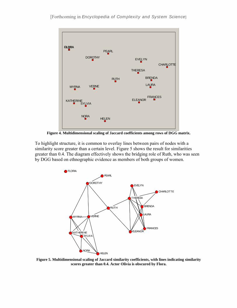
5.1 Unimodal Visualization of 2-Mode Data Given that a 2-mode matrix has been transformed into a 1-mode matrix by taking similarities among the rows (or columns), one can visualize the network using all the usual techniques for visualization of valued networks. For example, a standard approach is to use metric multidimensional scaling (MDS) on the matrix A, generating a map in which points corresponding to nodes (e.g., persons) appear close to each other to the extent that they share many groups. Figure 4 shows such an MDS map based on Jaccard similarities.


EVELYN

LAURA

THERESA

BRENDA

CHARLOTTE

FRANCESELEANOR

PEARL

RUTH

VERNEMYRNA

KATHERINESYLVIA

NORAHELEN

DOROTHY

OLIVIAFLORA

Figure 4. Multidimensional scaling of Jaccard coefficients among rows of DGG matrix.

To highlight structure, it is common to overlay lines between pairs of nodes with a similarity score greater than a certain level. Figure 5 shows the result for similarities greater than 0.4. The diagram effectively shows the bridging role of Ruth, who was seen by DGG based on ethnographic evidence as members of both groups of women.

EVELYN

LAURA

THERESA

BRENDA

CHARLOTTE

FRANCESELEANOR

PEARL

RUTH

VERNEMYRNA

KATHERINESYLVIA

NORAHELEN

DOROTHY

OLIVIAFLORA

Figure 5. Multidimensional scaling of Jaccard similarity coefficients, with lines indicating similarity

scores greater than 0.4. Actor Olivia is obscured by Flora.


Alternatively, one can use a standard graph layout algorithm (GLA) to draw the graph induced by dichotomizing the Jaccard similarity matrix. For example, define Evu ∈),( if and only if (iff) 4.0>ijc . Compared to multidimensional scaling representations, GLAs have the disadvantage that distances between points cannot strictly be interpreted, but this property also means that nodes need not obscure each other. Figure 6 shows the results of applying a spring-embedding (Kamada and Kawai, 1989) GLA to the dichotomized data.

EVELYN

LAURATHERESA

BRENDA

CHARLOTTE

FRANCES

ELEANOR

PEARL

RUTHVERNE

MYRNAKATHERINE

SYLVIA

NORA HELEN

DOROTHY

OLIVIAFLORA

Figure 6. Spring-embedding representation of Jaccard similarities dichotomized at > 0.4

A similar analysis can be carried out on the events rather than the women. Applying Equation 3 to the columns of the 2-mode matrix in Figure 1 yields a matrix of Jaccard coefficients which can be visualized using the same methods used for the women. Figure 7 shows events with Jaccard overlaps greater than 0.35.

E1

E2

E3

E4

E5

E6

E7

E8E9

E10

E11

E12E13

E14

Figure 7. Spring-embedding representation of “ties” among events ( 35.0>ijc ).

5.2 Unimodal Analysis of 2-Mode Data In general, analysis of 2-mode data transformed into valued 1-mode networks proceeds like any other valued network. As with visualization, this often means generating a graph from the valued data via some rule such as (u,v) ∈ E iff aij > q, where q is chosen by the researcher. Typically, there is no theoretical reason for choosing any particular value of q; hence a series of different values is generally chosen and the analysis repeated for each.


There are, however, a few consequences that stem from the 2-mode origin of the data. By their very nature, many commonly used measures of similarity and dissimilarity satisfy triangle inequality laws. For example, for Euclidean distance, every triple of nodes i, j, k satisfy the following rule: jkijik ddd +≤ Equation 5 As a result, the 1-mode data (especially if not dichotomized) artifactually exhibit a certain level of transitivity that may be higher than baseline models built on simple sociometric choice data would expect. Statistics based on transitivity, such as structural holes and clustering coefficients, must similarly be interpreted with some caution in such data. 6. Bimodal Approaches to 2-Mode Data Another approach to working with 2-mode data seeks to analyze both modes simultaneously. The data are seen to represent relations between two sets of nodes, forming a bipartite graph GB(V1+V2,E) in which, or all u and v, (u,v) ∈ E if and only if u and v belong to different vertex sets. In other words, all ties are between vertex sets and none are within-group. The matrix representation of such a graph can be a rectangular incidence matrix X (as in Figure 1) or a square bipartite adjacency matrix B with n=n1+n2 rows representing both modes, and an equal number of columns, also representing both modes. In the latter case, the original matrix X forms a submatrix of the larger adjacency matrix B in which both rows and columns index the V1+V2 entities. The matrix B is composed of four blocks, two of which are empty, as shown in Figure 8. Note that the original matrix X forms the top right quadrant of B, and its transpose forms the bottom left quadrant.

0 0 0 0 0 0 0 0 0 0 0 0 0 0 0 0 0 0 1 1 1 1 1 1 0 1 1 0 0 0 0 00 0 0 0 0 0 0 0 0 0 0 0 0 0 0 0 0 0 1 1 1 0 1 1 1 1 0 0 0 0 0 00 0 0 0 0 0 0 0 0 0 0 0 0 0 0 0 0 0 0 1 1 1 1 1 1 1 1 0 0 0 0 00 0 0 0 0 0 0 0 0 0 0 0 0 0 0 0 0 0 1 0 1 1 1 1 1 1 0 0 0 0 0 00 0 0 0 0 0 0 0 0 0 0 0 0 0 0 0 0 0 0 0 1 1 1 0 1 0 0 0 0 0 0 00 0 0 0 0 0 0 0 0 0 0 0 0 0 0 0 0 0 0 0 1 0 1 1 0 1 0 0 0 0 0 00 0 0 0 0 0 0 0 0 0 0 0 0 0 0 0 0 0 0 0 0 0 1 1 1 1 0 0 0 0 0 00 0 0 0 0 0 0 0 0 0 0 0 0 0 0 0 0 0 0 0 0 0 0 1 0 1 1 0 0 0 0 00 0 0 0 0 0 0 0 0 0 0 0 0 0 0 0 0 0 0 0 0 0 1 0 1 1 1 0 0 0 0 00 0 0 0 0 0 0 0 0 0 0 0 0 0 0 0 0 0 0 0 0 0 0 0 1 1 1 0 0 1 0 00 0 0 0 0 0 0 0 0 0 0 0 0 0 0 0 0 0 0 0 0 0 0 0 0 1 1 1 0 1 0 00 0 0 0 0 0 0 0 0 0 0 0 0 0 0 0 0 0 0 0 0 0 0 0 0 1 1 1 0 1 1 10 0 0 0 0 0 0 0 0 0 0 0 0 0 0 0 0 0 0 0 0 0 0 0 1 1 1 1 0 1 1 10 0 0 0 0 0 0 0 0 0 0 0 0 0 0 0 0 0 0 0 0 0 0 1 1 0 1 1 1 1 1 10 0 0 0 0 0 0 0 0 0 0 0 0 0 0 0 0 0 0 0 0 0 0 0 1 1 0 1 1 1 0 00 0 0 0 0 0 0 0 0 0 0 0 0 0 0 0 0 0 0 0 0 0 0 0 0 1 1 0 0 0 0 00 0 0 0 0 0 0 0 0 0 0 0 0 0 0 0 0 0 0 0 0 0 0 0 0 0 1 0 1 0 0 00 0 0 0 0 0 0 0 0 0 0 0 0 0 0 0 0 0 0 0 0 0 0 0 0 0 1 0 1 0 0 01 1 0 1 0 0 0 0 0 0 0 0 0 0 0 0 0 0 0 0 0 0 0 0 0 0 0 0 0 0 0 01 1 1 0 0 0 0 0 0 0 0 0 0 0 0 0 0 0 0 0 0 0 0 0 0 0 0 0 0 0 0 01 1 1 1 1 1 0 0 0 0 0 0 0 0 0 0 0 0 0 0 0 0 0 0 0 0 0 0 0 0 0 01 0 1 1 1 0 0 0 0 0 0 0 0 0 0 0 0 0 0 0 0 0 0 0 0 0 0 0 0 0 0 01 1 1 1 1 1 1 0 1 0 0 0 0 0 0 0 0 0 0 0 0 0 0 0 0 0 0 0 0 0 0 01 1 1 1 0 1 1 1 0 0 0 0 0 1 0 0 0 0 0 0 0 0 0 0 0 0 0 0 0 0 0 00 1 1 1 1 0 1 0 1 1 0 0 1 1 1 0 0 0 0 0 0 0 0 0 0 0 0 0 0 0 0 01 1 1 1 0 1 1 1 1 1 1 1 1 0 1 1 0 0 0 0 0 0 0 0 0 0 0 0 0 0 0 01 0 1 0 0 0 0 1 1 1 1 1 1 1 0 1 1 1 0 0 0 0 0 0 0 0 0 0 0 0 0 00 0 0 0 0 0 0 0 0 0 1 1 1 1 1 0 0 0 0 0 0 0 0 0 0 0 0 0 0 0 0 00 0 0 0 0 0 0 0 0 0 0 0 0 1 1 0 1 1 0 0 0 0 0 0 0 0 0 0 0 0 0 00 0 0 0 0 0 0 0 0 1 1 1 1 1 1 0 0 0 0 0 0 0 0 0 0 0 0 0 0 0 0 00 0 0 0 0 0 0 0 0 0 0 1 1 1 0 0 0 0 0 0 0 0 0 0 0 0 0 0 0 0 0 00 0 0 0 0 0 0 0 0 0 0 1 1 1 0 0 0 0 0 0 0 0 0 0 0 0 0 0 0 0 0 0

Figure 8. Bipartite adjacency matrix B created from the original

DGG 2-mode matrix X.


6.1 Bimodal Visualization of 2-Mode Data All of the standard ways to visualize networks, such as MDS and GLAs, apply to bipartite graphs. For example, Figure 9 shows a spring-embedding layout of the bipartite graph represented by the matrix in Figure 8.

EVELYN

LAURATHERESA

BRENDA

CHARLOTTE

FRANCESELEANOR

PEARL

RUTH

VERNE

MYRNA

KATHERINE

SYLVIA

NORA

HELEN

DOROTHY

OLIVIAFLORA

E1

E2

E3

E4

E5

E6

E7

E8

E9

E10

E11

E12

E13

E14

Figure 9. Spring-embedding representation of bipartite graph.

In the representation, two nodes are near each other roughly to the extent that the geodesic distance between them is short. Thus, events are near each other if they are attended by the same women (distance 2), and women are near each other if they attend the same events. In this example, the representation makes clear that there is a set of women on the left (Mryna, Helen, Katherine, Nora, Silvia, etc) that attend a set of events exclusive to them (events 10 through 13), and another set of women (Evelyn, Theresa, Laura, Brenda, etc) that have their own events (E1 through E4), and finally a set of events that both “circles” of women attend (events E6 through E9). For small datasets, this bimodal visualization is often extremely effective for transmitting a holistic understanding of the whole dataset. It is worth noting that there is a simple mathematical relationship between pairwise overlaps as aij as defined in Equation 1 and path lengths in the bipartite graph. Specifically, the number of 2-step paths between any pair of women i and j in the bipartite graph is equal to aij, the number of events they attended in common. Of course, the number of 2-step paths is simply the matrix product BB, the bipartite adjacency matrix multiplied by itself. As shown in Figure 10, the top left block and bottom right


blocks of BB are the matrices A as calculated by Equation 1 for rows and columns respectively of X.

EVE LAU THE BRE CHA FRA ELE PEA RUT VER MYR KAT SYL NOR HEL DOR OLI FLO E1 E2 E3 E4 E5 E6 E7 E8 E9 E10 E11 E12 E13 E14EVELYN 8 6 7 6 3 4 3 3 3 2 2 2 2 2 1 2 1 1 0 0 0 0 0 0 0 0 0 0 0 0 0 0LAURA 6 7 6 6 3 4 4 2 3 2 1 1 2 2 2 1 0 0 0 0 0 0 0 0 0 0 0 0 0 0 0 0THERESA 7 6 8 6 4 4 4 3 4 3 2 2 3 3 2 2 1 1 0 0 0 0 0 0 0 0 0 0 0 0 0 0BRENDA 6 6 6 7 4 4 4 2 3 2 1 1 2 2 2 1 0 0 0 0 0 0 0 0 0 0 0 0 0 0 0 0CHARLOTTE 3 3 4 4 4 2 2 0 2 1 0 0 1 1 1 0 0 0 0 0 0 0 0 0 0 0 0 0 0 0 0 0FRANCES 4 4 4 4 2 4 3 2 2 1 1 1 1 1 1 1 0 0 0 0 0 0 0 0 0 0 0 0 0 0 0 0ELEANOR 3 4 4 4 2 3 4 2 3 2 1 1 2 2 2 1 0 0 0 0 0 0 0 0 0 0 0 0 0 0 0 0PEARL 3 2 3 2 0 2 2 3 2 2 2 2 2 2 1 2 1 1 0 0 0 0 0 0 0 0 0 0 0 0 0 0RUTH 3 3 4 3 2 2 3 2 4 3 2 2 3 2 2 2 1 1 0 0 0 0 0 0 0 0 0 0 0 0 0 0VERNE 2 2 3 2 1 1 2 2 3 4 3 3 4 3 3 2 1 1 0 0 0 0 0 0 0 0 0 0 0 0 0 0MYRNA 2 1 2 1 0 1 1 2 2 3 4 4 4 3 3 2 1 1 0 0 0 0 0 0 0 0 0 0 0 0 0 0KATHERINE 2 1 2 1 0 1 1 2 2 3 4 6 6 5 3 2 1 1 0 0 0 0 0 0 0 0 0 0 0 0 0 0SYLVIA 2 2 3 2 1 1 2 2 3 4 4 6 7 6 4 2 1 1 0 0 0 0 0 0 0 0 0 0 0 0 0 0NORA 2 2 3 2 1 1 2 2 2 3 3 5 6 8 4 1 2 2 0 0 0 0 0 0 0 0 0 0 0 0 0 0HELEN 1 2 2 2 1 1 2 1 2 3 3 3 4 4 5 1 1 1 0 0 0 0 0 0 0 0 0 0 0 0 0 0DOROTHY 2 1 2 1 0 1 1 2 2 2 2 2 2 1 1 2 1 1 0 0 0 0 0 0 0 0 0 0 0 0 0 0OLIVIA 1 0 1 0 0 0 0 1 1 1 1 1 1 2 1 1 2 2 0 0 0 0 0 0 0 0 0 0 0 0 0 0FLORA 1 0 1 0 0 0 0 1 1 1 1 1 1 2 1 1 2 2 0 0 0 0 0 0 0 0 0 0 0 0 0 0E1 0 0 0 0 0 0 0 0 0 0 0 0 0 0 0 0 0 0 3 2 3 2 3 3 2 3 1 0 0 0 0 0E2 0 0 0 0 0 0 0 0 0 0 0 0 0 0 0 0 0 0 2 3 3 2 3 3 2 3 2 0 0 0 0 0E3 0 0 0 0 0 0 0 0 0 0 0 0 0 0 0 0 0 0 3 3 6 4 6 5 4 5 2 0 0 0 0 0E4 0 0 0 0 0 0 0 0 0 0 0 0 0 0 0 0 0 0 2 2 4 4 4 3 3 3 2 0 0 0 0 0E5 0 0 0 0 0 0 0 0 0 0 0 0 0 0 0 0 0 0 3 3 6 4 8 6 6 7 3 0 0 0 0 0E6 0 0 0 0 0 0 0 0 0 0 0 0 0 0 0 0 0 0 3 3 5 3 6 8 5 7 4 1 1 1 1 1E7 0 0 0 0 0 0 0 0 0 0 0 0 0 0 0 0 0 0 2 2 4 3 6 5 10 8 5 3 2 4 2 2E8 0 0 0 0 0 0 0 0 0 0 0 0 0 0 0 0 0 0 3 3 5 3 7 7 8 14 9 4 1 5 2 2E9 0 0 0 0 0 0 0 0 0 0 0 0 0 0 0 0 0 0 1 2 2 2 3 4 5 9 12 4 3 5 3 3E10 0 0 0 0 0 0 0 0 0 0 0 0 0 0 0 0 0 0 0 0 0 0 0 1 3 4 4 5 2 5 3 3E11 0 0 0 0 0 0 0 0 0 0 0 0 0 0 0 0 0 0 0 0 0 0 0 1 2 1 3 2 4 2 1 1E12 0 0 0 0 0 0 0 0 0 0 0 0 0 0 0 0 0 0 0 0 0 0 0 1 4 5 5 5 2 6 3 3E13 0 0 0 0 0 0 0 0 0 0 0 0 0 0 0 0 0 0 0 0 0 0 0 1 2 2 3 3 1 3 3 3E14 0 0 0 0 0 0 0 0 0 0 0 0 0 0 0 0 0 0 0 0 0 0 0 1 2 2 3 3 1 3 3 3

Figure 10. Matrix BB giving the number of paths of length 2 between all pairs of nodes.

6.2 Bimodal Analysis of 2-Mode Data Given a bimodal perspective, one approach to analyzing 2-mode data is to develop entirely new metrics and algorithms designed specifically for 2-mode data. Such techniques take cognizance of the fact that the observed network is not just bipartite by happenstance, but could not have been any other way. In other words, taking account of the fact that the observed lack ties between certain nodes (namely, those belonging to different modes) was by design – similar to the concept of structural zeros in log-linear modeling. To date, few techniques of this kind have been developed, the exception being the area of 2-mode centrality measures, which has received significant attention (e.g., Bonacich, 1991). Another approach is to treat the bipartite graphs as ordinary graphs and apply all the standard algorithms and techniques of social network analysis. Effectively this assumes either that the special nature of the graphs will not affect the techniques, or that we can pretend that ties within modes could have occurred and just didn’t. This approach works for a small class of methods, but by no means all. For example, calculating transitivity fails because transitive triples are impossible in bipartite graphs (all ties are between modes, which means that if a b and b c then a and c must be members of the same class, and therefore cannot be tied, making transitivity impossible). In contrast, if we were to adapt the definition of transitivity to be based on quadruples such that a quad is transitive if a b, b c, c d and a d, this would be an example of the first approach.


Finally, a compromise approach is to use the standard metrics and algorithms that apply to general graphs, and then either adjust the outputs via normalization or adjust the baseline expectations for the results (Borgatti and Everett, 1997; Faust, 1997). In the former case, we develop normalizations that adjust the metrics (typically by dividing by theoretical bipartite maxima), and in the latter case we derive different theoretical distributions for the statistics in question. In general, we choose the former approach when statistics are bounded between 0 and 1 and can be interpreted as proportions of maximum possible values. We choose the latter approach when the statistics are unbounded and have direct interpretations (see example of cohesion below). In this section, we can consider a mix of techniques drawn from these three approaches. 6.2.1 Bimodal Approaches to Graph Cohesion The simplest and most common measure of network cohesion is density – the number of edges divided by the number of pairs of nodes (using ordered pairs in the case of directed graphs and unordered pairs in the case of undirected graphs). In bipartite graphs, of course, only edges between vertex sets are possible. As a result, the maximum possible undirected ordinary density is

)1)(( 2121

21

−++ nnnnnn Equation 6

Thus, if density were calculated on a 2-mode network as if it were an ordinary graph, we would probably want to normalize the result by dividing by the sum above, otherwise the calculated density would appear misleadingly low. This is a case where the “compromise approach” discussed above is effective. (Of course, in terms of computation, it would be easier to simply calculate the average of the 2-mode matrix X rather than convert to bipartite form and then perform this adjustment.) For measures of cohesion that are not expressed as fractions of maximum possible values, such as average geodesic path length, the need to renormalize is not as great, since the raw values are directly interpretable. In doing so, however, we must be careful not to compare the results with standard rules of thumb or theoretical models based on simple random graphs, as these have not assumed the bipartite restrictions. 6.2.2 Bimodal Approaches to Centrality Four measures of centrality are used with high frequency in social network analysis today: degree, closeness, betweenness and eigenvector. We discuss each in turn. Degree centrality, di, is defined as the number of ties incident upon node i. Degree centrality is typically normalized by dividing by the maximum number of ties possible, which in a graph of n nodes is n-1. Hence

1*

−=

ndd i

i Equation 7


However, in any (non-trivial) bipartite graph, no node can be connected to all others, since this would mean within-mode ties. Instead, for a node in V1, the maximum number of ties it could have is n2, whereas for a node in V2, the maximum number of ties is n1. Hence a natural adjustment is to provide two separate normalization formulas as follows:

2

*

ndd i

i = , for 1Vi∈

1

*

nd

d jj = , for 2Vj∈

Equation 8

Closeness centrality is ordinarily defined as the sum of geodesic distances from a node to all others, as shown in Equation 8, where dij is the length of the shortest path from i to j and n = n1+n2 is the total number of nodes. The best (smallest) score possible occurs when the node has a tie to every other node, in which case the total distance to all others is n-1. Thus, closeness centrality is usually normalized by dividing ci into n-1.

∑=n

jiji dc

ii c

nc 1* −=

Equation 9

In the bipartite case, the maximum number of nodes that a node can be distance 1 from is the number of nodes in the other class. For other nodes in its own class, the closest it can be is two links away. Thus, the theoretical bipartite minimum value of ci (where 1Vi∈ ) is

)1(2 12 −+ nn and the minimum for cj (where 2Vj∈ ) is )1(2 21 −+ nn . Therefore, closeness centrality can be normalized in bipartite graphs as follows:

ii c

nnc )1(2 12* −+= , for 1Vi∈

jj c

nnc )1(2 21* −+= , for 2Vj∈

Equation 10

Betweenness centrality refers to the sum of shares of shortest paths that pass through a given node. The betweenness of node k in an ordinary graph is defined by Equation 11, where gij is the number of geodesic paths from node i to node j, and gikj is the number of geodesic paths from i to j that pass through k.

∑∑≠ ≠

=n

ki

n

ikj ij

ikjk g

gb

,21 Equation 11


Betweenness is ordinarily normalized by dividing by (n-1)(n-2) = n2 – 3n + 2, which is the maximum betweenness that any node can achieve in a graph with n nodes, which occurs for the node at the center of a star-shaped graph. This maximum is appropriate for bipartite graphs only when one mode has just one node; otherwise we must take account of the sizes of each vertex set. Equation 11 gives the maximums for nodes in each vertex set as a function of the vertex set sizes. In the equation, x div y refers to integer division of x by y and x mod y refers to the remainder of an integer division of x by y. )]32()12)(1()1([ 2

2222

1max1

+−−−−+++= tststsnsnbV

21 )1( ndivns −= , 21 mod)1( nnt −= )]32()12)(1()1([ 1

2212

1max2

+−−−−+++= rprprpnpnbV

12 )1( ndivnp −= , 21 mod)1( nnr −=

Equation 12

Given these maxima, we can normalize standard betweenness centrality for bipartite graphs by dividing by these maxima, as shown in Equation 13.

max

*

1V

ii b

bb = , for 1Vi∈

max

*

2V

jj b

bb = , for 2Vj∈

Equation 13

6.2.3. Cohesive Subgroups Detecting cohesive subgroups is somewhat more difficult in bipartite graphs than in ordinary graphs. For example, one of the earliest formal definitions of a subgroup is the clique (Luce and Perry, 1949) which is defined as a maximal complete subgraph – i.e., a set of nodes that is as large as possible subject to the condition that every pair is adjacent. However, in bipartite graphs, cliques are impossible, since in any connected triple, two nodes must be non-adjacent. Thus, cliques are not useful in this context. In addition, relaxations of the clique concept based on density or frequency of paths (such as k-plexes, lambda sets and ls-sets) do not work well, due to the sparse nature of bipartite graphs. For example, if we calculate k-plexes for the DGG dataset, we find huge numbers of very small groups. For k = 2, there are 394 2-plexes of size 3 or greater. For k = 3, there are 5,553 3-plexes, and for k = 4, there are 37,633 4-plexes of size 3 or greater. However, other classical notions of cohesive subgroups make more sense for bipartite graphs. In particular, relaxations of the clique concept based on distance, such as n-cliques, n-clans and n-clubs have good interpretations in bipartite graphs and work well in practice. In fact, 2-cliques defined on the bipartite graph have the property of bipartite completeness, meaning that, within the bipartite subgraph induced by the 2-clique, every node of one mode has a tie with every node of the other mode, which is to say that all possible ties are present. In this sense, for bipartite graphs, 2-cliques capture the underlying idea of a clique better than cliques do. This notion has been formalized in the definition of a biclique, which is defined as a maximal complete bipartite subgraph. Mathematically, it is identical to a 2-clique computed on the bipartite representation.


As a practical example, a biclique analysis of the DGG dataset finds 68 bicliques, and a secondary analysis of similarities of nodes across biclique membership profiles does a good job of revealing structure, as shown in Figure 11. In the figure, an edge is shown between two nodes if the Pearson correlation between their biclique membership profiles is greater than 0.4 (i.e., (u,v) ∈ E iff rij > 0.4). The two groups are women are clearly shown, as well as the two groups of events that are associated with each of the groups of women. In addition, the separation of Flora and Olivia is clearly shown, as well as the bridging position of Ruth and Pearl.

EVELYN

LAURA

THERESA

BRENDA

CHARLOTTEFRANCES

ELEANOR

PEARL

RUTHVERNE

MYRNA

KATHERINE

SYLVIA

NORA

HELEN

DOROTHY

OLIVIAFLORA

E1

E2

E3

E4

E5

E6E7E8E9

E10

E11

E12

E13

E14

Figure 11. Graph induced by Pearson correlations across biclique membership profiles. Edges

indicate a correlation greater than 0.4. The success of bicliques as 2-mode analogues of cliques suggests the possibility of creating 2-mode analogues for other cohesive subgroup concepts that we previously dismissed as unusable in the 2-mode context. For example, a k-plex is defined in ordinary network analysis as a maximal subgraph S(V,E) of size n such that each member of the k-plex is adjacent to at least n-k others. By analogy, for 2-mode networks we can define a (k1,k2)-biplex as a maximal bipartite subgraph G(V1,V2,E) such that each node in V1 is adjacent to |V2|-k2 others and each node in V2 is adjacent is adjacent to |V1|-k1 others. Obviously, a (0,0)-biplex is a biclique. A useful feature of this relaxation of a biclique is that we can set different standards of cohesiveness for each mode of the data network, perhaps reflecting the relative sizes of the modes, or the affiliative capabilities of the nodes themselves.


6.2.3. Bimodal Approaches to Positions and Roles Two concepts of position and role are particularly well known in social network analysis. These are structural equivalence and regular equivalence. Generalizations to 2-mode (and higher) data were developed by Borgatti (1989) and Borgatti and Everett (1992) and Everett and Borgatti (1993). We consider each of these in turn. 6.2.3.1 Structural Equivalence In the best definition of structural equivalence (Everett and Borgatti, 1994), two nodes u and v are said to be structurally equivalent if there exists a graph automorphism that would be an identity except that u and v are mapped to each other. In other words, given a diagram of the graph, you could swap nodes u and v (and no other nodes) without changing the structure of the network one iota. A key implication of this definition is that structurally equivalent nodes have identical relational environments – aside from each other, they are connected and not connected to exactly the same third parties. As a result, one approach to identifying structurally equivalent nodes is to compute a similarity measure among rows and columns of the adjacency matrix defining the graph. This approach requires no modification for the bipartite case. In fact, the unimodal analysis described in Section 5 (applied to each mode in turn) is precisely the same as computing structural equivalence on the 2-mode incidence matrix (Figure 1). In addition, for certain measures such as the Jaccard coefficient, computing structural equivalence on the bipartite adjacency matrix B of Figure 8 gives exactly the same results as computing it on the 2-mode incidence matrix X. Another approach to structural equivalence is known as blockmodeling. Instead of (or as a result of) measuring the extent of structural equivalence between nodes, we partition the nodes into classes such that nodes in the same class are structurally equivalent (or nearly so). Given such a partition of nodes, we can reorder and partition the corresponding rows and columns of the adjacency matrix. This in turn induces to partition of matrix cells into matrix blocks. A characteristic property of perfect structural equivalence partitions is that matrix blocks are necessarily homogeneous with respect to cell values, and each block will consist of all 1s or all 0s (known as 1-blocks and 0-blocks respectively). Figure 12 gives an example with three equivalence classes.


A1 A2 A3 B1 B2 B3 B4 C1 C2 C3A1 0 0 0 1 1 1 1 0 0 0A2 0 0 0 1 1 1 1 0 0 0A3 0 0 0 1 1 1 1 0 0 0B1 1 1 1 0 0 0 0 1 1 1B2 1 1 1 0 0 0 0 1 1 1B3 1 1 1 0 0 0 0 1 1 1B4 1 1 1 0 0 0 0 1 1 1C1 1 1 1 1 1 1 1 0 0 0C2 1 1 1 1 1 1 1 0 0 0C3 1 1 1 1 1 1 1 0 0 0

Figure 12. Perfect structural equivalence blockmodel.

In the 2-mode case, one approach is to blockmodel the bipartite adjacency matrix B. This can be done, but the bipartite structure imposes certain constraints. For example, blocks involving within-mode ties must be 0-blocks. In addition, the best 2-block partition will almost certainly be the mode partition (except in trivial cases), and in general, all other partitions will be refinements of the mode partition (i.e., they will be nested hierarchically within the mode partition). A more elegant (and computationally efficient) approach is to work from the 2-mode incidence matrix X. In this case, we redefine a blockmodel to refer to a coordinated pair of partitions, one for the rows and one for the columns. We then redefine structural equivalence as follows. Given a 2-mode matrix X with modes V1 and V2, a 2-mode blockmodeling P is said to be a structural equivalence if for all nodes u,v in Vi and all w in Vj, p(u) = p(v) iff xuw = xvw for i ≠ j and where p(u) indicates the equivalence class of node u. Restating this in words, a 2-mode structural equivalence blockmodeling is one in which row nodes in the same class if and only if they have identical rows, and column nodes are in the same class if and only if they have identical columns. An example involving 4 classes of rows and 3 classes of columns is shown in Figure 13.

E1 E2 E3 F1 F2 F3 F4 G1 G2 G3A1 1 1 1 1 1 1 1 0 0 0A2 1 1 1 1 1 1 1 0 0 0A3 1 1 1 1 1 1 1 0 0 0B1 1 1 1 0 0 0 0 0 0 0B2 1 1 1 0 0 0 0 0 0 0B3 1 1 1 0 0 0 0 0 0 0B4 1 1 1 0 0 0 0 0 0 0C1 0 0 0 1 1 1 1 0 0 0C2 0 0 0 1 1 1 1 0 0 0C3 0 0 0 1 1 1 1 0 0 0D1 0 0 0 1 1 1 1 1 1 1D2 0 0 0 1 1 1 1 1 1 1

Figure 13. A 2-mode structural equivalence blockmodel in which the row partition has 4 classes and

the column partition has 3 classes.


In empirical work, of course, we do not expect to obtain perfect 1-blocks and 0-blocks. Instead we seek partitions that minimize the number of errors (where we define an error as either a 1 inside a 0-block or a 0 inside a 1-block). 6.2.3.2 Regular Equivalence Two nodes are said to be regularly equivalent (i.e., play the same structural role) to each other to the extent that they have ties (lack of ties) to corresponding others who are themselves regularly equivalent to each other. That is, u and v are regularly equivalent if, (a) for all x such that u has a tie to x, there exists a y that is regularly equivalent to x such that v has a tie to y, and (b) for all x such that u has an incoming tie from x, there exists a y that is regularly equivalent to x such that v has an incoming tie from y. Whereas in structural equivalence equivalent nodes are connected to the same others, in regular equivalence equivalent nodes are connected to the same types of others. Alternatively, we can define regular equivalence in terms of a partition C of nodes into labeled classes (known as colors) such that regularly equivalent nodes are required to have the same colors in their neighborhoods. That is, for all nodes u and v, C(u) = C(v) implies C(N(u)) = C(N(v)), Equation 14 where C(N(u)) is the set of distinct colors found among the nodes constituting u’s immediate neighborhood.1 Taking a blockmodeling perspective, it can readily be seen that Equation 14 implies a blockmodel in which each matrix block is either entirely zero (a “zeroblock”) or contains at least one 1 in every column and in every row (a “regular oneblock”), as illustrated in Figure 14.

N1 N2 N3 N4 N5 N6 N7 N8 N9 N10N1 0 0 0 1 0 0 1 0 0 0N2 0 0 0 0 1 0 0 0 0 0N3 0 0 0 1 1 1 1 0 0 0N4 1 0 0 0 0 0 0 0 1 1N5 1 0 1 0 0 0 0 1 1 0N6 0 1 0 0 0 0 0 0 1 1N7 0 1 1 0 0 0 0 1 0 1N8 1 0 1 0 1 1 0 0 0 0N9 0 0 1 0 0 1 0 0 0 0N10 0 1 0 1 1 0 1 0 0 0

Figure 14. Perfect regular equivalence blockmodel on an ordinary graph.

1 For directed graphs, we require C(No(u)) = C(No(v)) and C(Ni(u)) = C(Ni(v)), where No(v) refers to the set of nodes that v sends a tie to, and Ni(u) refers to the set of nodes that v receives a tie from.


Equation 14 lends itself easily to the bipartite case. Instead of seeking a single partition of nodes, we seek a different partition for each mode. Labeling these partitions R and C, we modify our definition such that for all u,v ∈ V1 and x,y ∈ V2, C(u) = C(v) implies R(N(u)) = R(N(v)),

and R(x) = R(y) implies C(N(x)) = C(N(y)).

Equation 15

Of course, the neighbors N() of any node consist entirely of nodes belonging to the other mode. Thinking in terms of the 2-mode incidence matrix shown in Figure 1, Equation 15 implies that we can section the matrix into rectangular blocks such that each block is zeroblock or a regular 1-block. An example of a 2-mode regular blockmodel is shown in Figure 15.

Figure 15. A 2-mode regular equivalence blockmodel. As with structural equivalence, in empirical work we do not expect to obtain perfect 1-blocks and 0-blocks. Instead we seek partitions induce matrix blocks that are as nearly regular as possible. 7. Conclusion In this chapter we have considered methods of visualizing and analyzing 2-mode network data. An examination of the chapter suggests that four strategies are employed for handling 2-mode data. First, there is converting the data into two separate 1-mode datasets, and analyzing each separately. Second, there is using existing 1-mode methods on a bipartite representation of the 2-mode data, and essentially ignoring its special features. Third, there is using 1-mode methods but either adjusting the interpretation or applying some kind of normalization to adjust the results. Finally, there is developing new methods designed specifically for the 2-mode case. The chapter has provided examples of all four strategies.

R1 R2 R3 R4 R5 R6 R7 R8 R9 R10C1 1 0 1 0 1 1 0 0 0 0C2 0 0 1 0 0 1 0 0 0 0C3 0 1 0 1 1 0 1 0 0 0C4 1 0 0 0 0 0 0 0 1 1C5 1 0 1 0 0 0 0 1 1 0C6 0 1 0 0 0 0 0 0 1 1C7 0 1 1 0 0 0 0 1 0 1C8 0 0 0 0 1 1 0 0 0 0C9 0 0 0 0 0 1 0 0 0 0C10 0 0 0 1 1 0 1 0 0 0C11 1 0 1 0 0 0 0 0 1 1C12 0 1 0 0 0 0 0 1 0 1


It is worth reminding the reader that only 2-mode data viewed in a network context has been considered here. In principle, most data dealt with by social scientists is structured as a 2-mode matrix of cases (rows) and variables (columns) and most statistical techniques assume such data. This chapter obviously does not discuss this vast pantheon of techniques, although it is clear that many would be appropriate, particularly structure-finding techniques such as factor analysis and correspondence analysis. 8. Future Directions Although it would be a mistake to think of 2-mode data as an advance over 1-mode data, it is important to note that there are many cases were extending network analysis methodology to more than 2 modes is desirable. For example, we might analyze membership in organizations over time, yielding a 3-way, 3-mode data matrix of relations that is person by organization by period. Similarly, we might be interested in modeling the intellectual landscape of an academic field, representing publications as k-mode bundles of authors, journals, years, institutional affiliations and topics. References Bonacich P. 1972 'Techniques for analyzing overlapping memberships' Sociological Methodology 176-185 Jossey-Bass. Bonacich, Phillip. 1991. Simultaneous group and individual centralities. Social Networks 13, 155-168. Borgatti, S. P. 1989. Regular equivalence in graphs, hypergraphs, and matrices. Doctoral Dissertation, Univ. of California, Irvine. Ann Arbor: UMI. Borgatti, S. P., & Everett, M. G. 1992. Regular blockmodels of multiway, multimode matrices. Social Networks, 14: 91-120. Borgatti, S. P., & Everett, M. G. 1997. Network analysis of 2-mode data. Social Networks, 19(3): 243-269 Davis, A., B. Gardner and M. Gardner 1941 Deep South: A Social Anthropological Study of Caste and Class. Chicago: University of Chicago Press. Everett, M. G., & Borgatti, S. P. 1993. An extension of regular colouring of graphs to digraphs, networks and hypergraphs. Social Networks, 15: 237-254 Everett, M.G., & Borgatti, S. P. 1994. Regular equivalence: General theory. Journal of Mathematical Sociology, 19(1): 29-52. Faust, K. 1997. "Centrality in affiliation networks." Social Networks 19:157-191


Luce, R.D. and A.D. Perry. 1949. A method of matrix analysis of group structure. Psychometrika. 20, 319-327

2-Mode Concepts in Social Network Analysis - Steve …steveborgatti.com/papers/2modeconcepts.pdf · 2-Mode Concepts in Social Network Analysis ... In social network analysis, 2-mode

Documents