2. Introduction to Probability 2015 - UMass Amherstpeople.umass.edu/biep540w/pdf/2. Introduction to Probability 2015.pdf · BIOSTATS 540 – Fall 2015 2. Introduction to Probability

BIOSTATS 540 – Fall 2015 2. Introduction to Probability Page 1 of 53

Nature Population/ Sample

Observation/ Data

Relationships/ Modeling

Analysis/ Synthesis

Unit 2 Introduction to Probability

“Chance favours only those who know how to court her”

- Charles Nicolle

A weather report statement such as “the probability of rain today is 50%” is familiar and we have an intuition for what it means. But what does it really mean? Our intuitions about probability come from our experiences of relative frequencies of events. Counting! This unit is a very basic introduction to probability. It is limited to the “frequentist” approach. It’s important because we hope to generalize findings from data in a sample to the population from which the sample came. Valid inference from a sample to a population is best when the probability framework that links the sample to the population is known.



Observation/ Data


Analysis/ Synthesis

Table of Contents Topics

1. Unit Roadmap …………………………………………………………….. 2. Learning Objectives ………………………………………………………. 3. Why We Need Probability ………….……………..………………..……… 4. The Basics: Some Terms Explained………..……………………………… a. “Frequentist” versus “Bayesian” versus “Subjective”………..………… b. Sample Space, Elementary Outcomes, Events ………………………… c. “Mutually Exclusive” and “Statistical Independence” …………………. d. Complement, Union, and Intersection ………………………………… e. The Joint Probability of Independent Events ………………………….. 5. The Basics: Introduction to Probability Calculations …………………… “Equally Likely” Setting - ………………………………………………. 6. The Addition Rule ……....…………………………..…..………………… 7. The Multiplication Rule - The Basics ……..……………………………… 8. Conditional Probability ………………………………..…………………. a. Terms Explained: Independence, Dependence, Conditional Probability b. The Multiplication Rule – A little More Advanced ……………………. c. TOOL - The Theorem of Total Probability ……………………….…… d. TOOL - Bayes Rule ………………..…………………………….…… 9. Probabilities in Practice - Screening Tests and Bayes Rule …….………..… a. Prevalence…………………………………………………………...

b. Incidence ………………………………….……………..…..….…. c. Sensitivity, Specificity ………………………………………….… d. Predictive Value Positive, Negative Test ……………………….…

10. Probabilities in Practice - Risk, Odds, Relative Risk, Odds Ratio …....

a. Risk ………………………………………………………...…….. b. Odds ………………………………..……………………..……… c. Relative Risk ………………………………………………….…… d. Odds Ratio …………………………………………….………...…

Appendices 1. Some Elementary Laws of Probability ……………………….…… 2. Introduction to the Concept of Expected Value .………….…………

3

4

5

7 7 8

10 12 14

15 15

21

24

25 25 28 30 32

35 35 35 36 39

41 41 43 45 46

49 52



Observation/ Data


Analysis/ Synthesis

1. Unit Roadmap

Nature/

Populations

In Unit 1, we learned that a variable is something whose value can vary. A random variable is something that can take on different values depending on chance. In this context, we define a sample space as the collection of all possible outcomes for a random variable. Note – It’s tempting to call this collection a ‘population.’ We don’t because we reserve that for describing nature. So we use the term “sample space” instead. An event is one outcome or a set of outcomes. Gerstman BB defines probability as the proportion of times an event is expected to occur in the population. It is a number between 0 and 1, with 0 meaning “never” and 1 meaning “always.”

Unit 2. Introduction to Probability

Sample

Observation/ Data

Relationships

Modeling

Analysis/ Synthesis



Observation/ Data


Analysis/ Synthesis

2. Learning Objectives

When you have finished this unit, you should be able to:

§ Define probability, from a “frequentist” perspective.

§ Explain the distinction between outcome and event.

§ Calculate probabilities of outcomes and events using the proportional frequency approach.

§ Define and explain the distinction among the following kinds of events: mutually exclusive, complement, union, intersection.

§ Define and explain the distinction between independent and dependent events.

§ Define prevalence, incidence, sensitivity, specificity, predictive value positive, and predictive value negative.

§ Calculate predictive value positive using Bayes Rule.

§ Defined and explain the distinction between risk and odds. Define and explain the distinction between relative risk and odds ratio.

§ Calculate and interpret an estimate of relative risk from observed data in a 2x2 table.

§ Calculate and interpret an estimate of odds ratio from observed data in a 2x2 table.



Observation/ Data


Analysis/ Synthesis

3. Why We Need Probability

In unit 1 (Summarizing Data), our scope of work was a limited one, describe the data at hand. We learned some ways to summarize data:

• Histograms, frequency tables, plots; • Means, medians; and • Variance, SD, SE, MAD, MADM.

And previously, (Course Introduction), we saw that, in our day to day lives, we have some intuition for probability.

• What are the chances of winning the lottery? (simple probability) • From an array of treatment possibilities, each associated with its own costs and prognosis, what is the optimal therapy? (conditional probability)

Chance - In these settings, we were appealing to “chance”. The notion of “chance” is described using concepts of probability and events. We recognize this in such familiar questions as:

• What are the chances that a diseased person will obtain a test result that indicates the same? (Sensitivity) • If the experimental treatment has no effect, how likely is the observed discrepancy between the average response of the controls and the average response of the treated? (Clinical Trial)



Observation/ Data


Analysis/ Synthesis

To appreciate the need for probability, consider the conceptual flow of this course:

• Initial lense - We are given a set of data. We don’t know where it came from. In summarizing it, our goal is to communicate its important features. (Unit 1 – Summarizing Data)

• Enlarged lense – Suppose now that we are interested in the population that gave rise to the sample. We ask how the sample was obtained. (Unit 3 – Populations and Samples).

• Same enlarged lense – If the sample was obtained using a method in which every possible sample is

equally likely (this is called “simple random sampling”), we can then calculate the chances of particular outcomes or events (Unit 2 – Introduction to Probability).

• Sometimes, the data at hand can be reasonably modeled as being a simple random sample from a particular population distribution – eg. - Bernoulli, Binomial, Normal. (Unit 4 – Bernoulli and Binomial Distribution, Unit 5 – Normal Distribution).

• Estimation – We use the values of the statistics we calculate from a sample of data as estimates of the unknown population parameter values from the population from which the sample was obtained. Eg – we might want to estimate the value of the population mean parameter (µ) using the value of the sample mean X (Unit 6 – Estimation and Unit 9-Correlation and Regression).

• Hypothesis Testing –We use calculations of probabilities to assess the chances of obtaining data summaries such as ours (or more extreme) for a null hypothesis model relative to a competing model called the alternative hypothesis model. (Unit 7-Hypothesis Testing, Unit 8 –Chi Square Tests)

Going forward:

• We will use the tools of probability in confidence interval construction.

• We will use the tools of probability in statistical hypothesis testing.



Observation/ Data


Analysis/ Synthesis

4. The Basics – Some Terms Explained

4a. “Frequentist” versus “Bayesian” versus “Subjective A Frequentist Approach -

• Begin with a sample space: This is the collection of all possible outcome values of sampling from a population. Example – A certain population of university students consists of 53 men and 47 women. Tip – Populations versus Sample Spaces: A collection of all possible individuals in nature is termed a “population”. The collection of all possible outcomes of sampling the population is termed a “sample space” • Suppose that we can do sampling of the population by the method of simple random sampling many times. (more on this in Unit 3, Populations and Samples). Example continued - What are our chances of selecting a female student? Call this our event of interest: “A.” • As the number of simple random samples drawn increases, the proportion of samples in

which the event “A” occurs eventually settles down to a fixed proportion. This eventual fixed proportion is an example of a limiting value. Example, continued – After 10 simple random samples, the proportion of samples in which gender=female might be 6/10, after 20 simple random samples, it might be 10/20, after 100 it might be 41/100, and so on. Eventually, with simple random sampling, the proportion of samples in which gender=female will reach its limiting value of .47

• The probability of event “A” is the value of the limiting proportion (percent of times). Example, continued – Probability [ A ] = .47

Again - This is a “frequentist” approach to probability. It is just one of three approaches.

• Bayesian - “This is a fair coin. It lands “heads” with probability 1/2. • Frequentist – “In 100 tosses, this coin landed heads 48 times”. • Subjective - “This is my lucky coin”.



Observation/ Data


Analysis/ Synthesis

4b. Sample Space, Elementary Outcomes, Event The sample space is comprised of all the possible outcomes of sampling of a population. Each of the possible outcomes in this scenario is also called an “elementary outcome”. What we are interested in might be an elementary outcome or it might be some collection of outcomes. Either way, we’ll use the term “event” to refer to what is of interest. Sample Space - The sample space is defined as the set of all possible (elementary) outcomes of sampling. I’m representing a sample space with a parallelogram that looks like this à I’m representing an (elementary) outcome with a dark circle that looks like this à Elementary Outcome (Sample Point), Each possible outcome of the sampling from the sample space is called an elementary outcome. Example – In this example, the outcome of sampling is a pair defined as { sex of 1st born twin, sex of 2nd born twin} There are exactly 4 possibilities: (boy,boy), (boy, girl), (girl, boy), (girl, girl). à Thus, the sample space is comprised of these 4 possibilities. Each of the 4 possible paired outcomes constitutes an elementary outcome. Definition Elementary Outcome: = {sex 1st twin, sex 2nd twin} Definition Sample Space: All 4 possible elementary outcomes:

{ boy, boy } { boy, girl } { girl, boy } { girl, girl }



Observation/ Data


Analysis/ Synthesis

Event -

Often, our interests are a bit broader than the elementary outcomes. For example, what if we want to know the probability of a boy? Snag. “Boy” isn’t an elementary outcome. But it is a realizable event! In particular, any of 3 elementary outcomes qualify as constituting the occurrence of a boy: (boy, boy), (boy, girl) and (girl, boy). Thus, the outcome of a “boy” is an example of an event. An event “E” is a collection of one or more elementary outcomes “O”. Notation - Notice that the individual outcomes or elementary sample points are denoted O1, O2, … while events are denoted E1, E2, …

Example, putting it all togther – In the language of these notes, we now say that we are interested in the event of “boy”. The event of a boy is satisfied when any of three elementary outcomes has occurred. The three qualifying elementary outcomes are the following:

{ boy, boy } { boy, girl } { girl, boy }

Example – continued Here are some more examples of “events”, together with their associated collections of qualifying elementary outcomes: Notation Event Qualifying elementary outcomes E1 “boy” {boy, boy} {boy, girl} {girl, boy} E2 “two boys” {boy, boy} E3 “two girls” {girl, girl} E4 “one boy, one girl” {boy, girl} {girl, boy}



Observation/ Data


Analysis/ Synthesis

4c. “Mutually Exclusive” and “Statistical Independence” Explained

The ideas of mutually exclusive and independence are different and can be confusing. The ways we work with them are also different. Mutually Exclusive (“cannot occur at the same time”) Here’s a mind numbingly boring example …. Nevertheless, it makes the point. A single coin toss cannot land heads and tails at the same time. So we say: A coin landed “heads” excludes the possibility that the coin landed “tails”. And then we say: The outcomes “heads” and “tails” in the outcome of a single coin toss are mutually exclusive. Two events are mutually exclusive if they cannot occur at the same time. Every day Examples of Mutually Exclusive –

• The weight of a single individual cannot be simultaneously “underweight”, “normal”, “overweight.” à These 3 events are mutually exclusive.

• Similarly, the race/Ethnicity of a single individual cannot be simultaneously “White Caucasian”, “African American”, “Latino”, “Native African”, “South East Asian”, “Other”. à These 6 events are mutually exclusive.

• The gender of a single individual cannot be simultaneously “Female”, “Male”, “Transgender” à These 3 events are mutually exclusive.



Observation/ Data


Analysis/ Synthesis

Statistical Independence (“the occurrence of the first does not change the chances of the second”) It’s not a perfect strategy but it’s a workable one – Think time. Consider three sets of paired events. Eg.-

• Individual is male with red hair. Paired event = [male gender, red hair]. The forces that determine hair being red might be independent of those that determine gender.

• Individual is young in age with high blood pressure. Paired event = [young age, high blood pressure]. The biology that produces high blood pressure might be independent of age.

• First coin toss yields “heads” and second, subsequent, coin toss yields “tails”. Paired event = [heads on 1st toss, tails on 2nd toss] The influences (wind, trajectory, etc) that determine the 2nd toss landing heads might be independent of those that determined the 1st toss landing heads.

Two events are statistically independent if the chances, or likelihood/probability, of one event is in no way related to the likelihood of the other event. We’ll get to calculating chances or likelihoods/probabilities in the next section. Here, consider the game of tossing one coin once and then tossing that same coin a second time. So what are the chances of two heads? This is familiar; it is 50% x 50%, representing a 25% chance. This is a simple example of statistical independence. By the definition of statistical independence (and its applicability to this silly example of a single fair coin): “Chances of two heads” = Pr[1st toss lands heads AND 2nd toss lands heads] = Pr[1st toss lands heads] x Pr[2nd toss lands heads] = .50 x .50 = .25 Thus, the distinction between “mutually exclusive” and “statistical independence” can be appreciated by incorporating an element of time. Mutually Exclusive (“cannot occur at the same time”) “heads on 1st coin toss” and “tails on 1st coin toss” are mutually exclusive. Probability [“heads on 1st” and “tails on 1st” ] = 0 Statistical Independence (“the first does not influence the subsequent occurrence of the later 2nd”) “heads on 1st coin toss” and “tails on 2nd coin toss” are statistically independent Probability [“heads on 1st” and “tails on 2nd ” ] = (1/2) (1/2)



Observation/ Data


Analysis/ Synthesis

4d. Complement, Union, Intersection Complement (”the opposite occurred”) - The complement of an event E is the event consisting of all outcomes in the population or sample space that are not contained in the event E. The complement of the event E is denoted using a superscript c, as in Ec Example – For the twins example, consider the event E2 = “two boys” that is introduced on page 10. The complement of the event E2 is denoted E2

c and is comprised of 3 elementary outcomes: E2

c = { boy, girl }, { girl, boy }, { girl, girl } Union, A or B (”either A occurred OR B occurred OR both A and B occurred”) - The union of two events, say A and B, is another event which contains those outcomes which are contained either in A or in B. The notation used is A ∪ B.



Observation/ Data


Analysis/ Synthesis

Example – For the twins example, consider the event (this is actually an elementary outcome) {boy, girl }. Call this “A”. Call “B” the event { girl, boy }. The union of events A and B is: A ∪ B = { boy, girl }, { girl, boy } Intersection, A and B (”only what is common to both A and B occurred”) - The intersection of two events, say A and B, is another event which contains only those outcomes which are contained in both A and in B. The notation used is A ∩ B. Here it is depicted in the color gray.

Example – For the twins example, consider next the events E1 defined as “having a boy” and E2 defined as “having a girl”. Thus, E1 = { boy, boy }, { boy, girl }, { girl, boy } E2 = { girl, girl }, { boy, girl }, { girl, boy } These two events do share some common outcomes. I’ve highlighted them in bold. The intersection of E1 and E2 is “having a boy and a girl”: E1 ∩ E2 = { girl, boy }, { boy, girl }



Observation/ Data


Analysis/ Synthesis

4e. The Joint Probability of Independent Events Independence, Dependence and conditional probability are discussed in more detail later. But we need a little bit of discussion of independent events here. Specifically,

If the occurrence of event E1 is independent of the occurrence of event E2, Then the probability that they BOTH occur is given by multiplying together the two probabilities: Probability [E1 occurs and E2 occurs ] = Pr[E1] x Pr[E2]

Example – The probability that two tosses of a fair coin both yield heads is ½ x ½ = ¼. chance. E1 = Outcome of heads on 1st toss. Pr[E1] = .50 E2 = Outcome of heads on 2nd toss Pr[E2] = .50 Pr[both land “heads”] = Pr[heads on 1st toss AND heads on 2nd toss ] = = Pr[heads on 1st toss] x Pr[heads on 2nd toss] = Pr[E1] x Pr[E2] = (.50)(.50) = .25



Observation/ Data


Analysis/ Synthesis

5. The Basics – Introduction to Probability Calculations The Equally Likely Setting In the “frequentist” framework, discrete probability calculations (these are also calculations of chance) are extensions of counting! We count the number of times an event of interest actually occurred, relative to how many times that event could possibly have occurred. For now, we consider the scenario in which every elementary outcome in the sample space is equally likely - • Consider again the population of 100 university students comprised of 53 men and 47 women. • We select one student from this population by the method of simple random sampling (Imagine. All the students are put into a big pot. The pot is stirred. We reach into the pot and select one). Each of the 100 students has the same (1 in 100) chance of being selected. “Simple random sampling” here means that each of the 100 students has the same (1 in 100) chance of being selected. à Equally likely refers to the common 1 in 100 chance of selection that each student has. • What if we want to know the chances of selecting a male? Or, the chances of selecting a female? This is our event of interest. We can define a random variable from this event. To do this: 1) list out all the possible values of the random variable. Answer – male, female. 2) For each, identify all the “qualifying” equally likely elementary outcomes. Answer - Easy in this example. They are the same. 3) The probability of each random variable value is obtained by adding together the probabilities of the associated elementary outcomes. Example – continued. We’ll call this new random variable X.

X = gender of selected individual student.

And, rather than having to write out “male” and “female”, we’ll use “0” and “1” as their representations, respectively. Thus, for convenience, we will say

X = 0 when the student selected is “male” X = 1 when the student selected is “female”



Observation/ Data


Analysis/ Synthesis

• From an initial collection of equally likely elementary outcomes (each of 100 students has an equal, 1 in 100, chance of being selected), together with a defined event of interest (the student selected is male) , we can now define what is called a discrete random variable. And we can state its probability distribution. The probability distribution of a discrete random variable is defined by a listing of all the possible outcomes (this is the sample space), together with the associated chances of occurrence (this is the probability model). Discrete Random Variable X = Gender of Selected Student Sample Space List of all the possible outcomes

Probability Model List of all the associated chances of occurrence

0 = male 1 = female

Tip! Be sure to check that this listing of all possible outcomes is truly “exhaustive”.

0.53 0.47 Be sure to check that all these probabilities add up to 100% or a total of 1.00.



Observation/ Data


Analysis/ Synthesis

Some More Formal Language

1. For a discrete random variable (we’ll get to continuous random variables later), a probability model is the set of assumptions used to assign probabilities to each possible value (realization) of the random variable. The sample space for the discrete random variable is the collection, of all the possible values that that random variable can have.

2. A probability distribution defines the relationship between the outcomes and their likelihood of occurrence.

3. To define a probability distribution, we make an assumption (the probability model) and use this to assign likelihoods.

4. When the values of a random variable are all equally likely, the probability model is called a uniform probability model.

Example #1 of a Uniform Probability Distribution – Role ONE die exactly ONE time Random Variable X = “face” of die Sample Space List of all the possible outcomes


1 2 3 4

5 6

Check! This listing of all possible outcomes is “exhaustive”.

1/6 1/6 1/6 1/6

1/6 1/6

Check! These probabilities total 1 or 100%.



Observation/ Data


Analysis/ Synthesis

Example #2 of a Uniform Probability Distribution – Toss ONE fair coin exactly ONE time Random Variable X = “face” of coin Sample Space List of all the possible outcomes


heads tails Check! This listing of all possible outcomes is “exhaustive”.

1/2 1/2 Check! These probabilities total 1 or 100%.

Example #3 of a Uniform Probability Distribution (Sampling With Replacement) – Select 1 digit, by simple random sampling from the list: 1, 2, 3. Return it. Then select a 2nd digit, by equal random sampling from the same list: 1, 2, 3.. N = size of list. n=size of sample. Random Variable X = {1st selected digit, 2nd selected digit} Sample Space (Size is 32 or Nn) List of all the possible outcomes


1,1 1,2 1,3 2,1

2,2 2,3 3,1

3,2 3,3 Check! This listing of all possible outcomes is “exhaustive”.

1/9 1/9 1/9 1/9

1/9 1/9

1/9 1/9 1/9 Check! These probabilities total 1 or 100%.



Observation/ Data


Analysis/ Synthesis

Example #4 of a Uniform Probability Distribution (Sampling Without Replacement) – Select 1 digit, by simple random sampling from the list: 1, 2, 3. Do not return it. Then select a 2nd digit, by equal random sampling from the remaining 2 numbers in the list. N = size of list. n=size of sample. Random Variable X = {1st selected digit, 2nd selected digit} Sample Space (Size is 3x2x1 or N x (N-1) x … x (N-n+1) List of all the possible outcomes


1,2 1,3 2,1 2,3

3,1 3,2

Check! This listing of all possible outcomes is “exhaustive”.

1/6 1/6 1/6 1/6

1/6 1/6

Check! These probabilities total 1 or 100%.

Tip – More on the ideas of “with replacement” and “without replacement” later.



Observation/ Data


Analysis/ Synthesis

How to Calculate Probability [Events “E”] in the Equally Likely Setting Now you know how to do this: – Add up the probabilities of the qualifying elementary outcomes. Example – Toss one coin two times. Assume that, for each toss, the coin lands heads or tails with the same probability = .50. Assume also that the outcomes of the two tosses are independent (the outcome of the 2nd toss is not influenced or changed in any way depending on the outcome of the 1st toss). Each elementary outcome is a pair = (1st coin face, 2nd coin face) Event , E Set of Qualifying Outcomes, O P(Event, Ei) E1: 2 heads {HH} ¼ = .25 E2: Just 1 head {HT, TH} ¼ + ¼ = .50 E3: 0 heads {TT} ¼ = .25 E4: Both the same {HH, TT} ¼ + ¼ = .50 E5: At least 1 head {HH, HT, TH} ¼ + ¼ + ¼ = .75



Observation/ Data


Analysis/ Synthesis

6. The Addition Rule

When to Use the Addition Rule Tip – Think “or” Use the addition rule when you want to calculate the event that either “A” occurs or “B” occurs or both occur. Example 1 – Starbucks will give you a latte with probability = .15. Suppose that independent of Starbucks, Dunkin Donuts will give you a donut with probability = .35. What are the chances that you will get a latte OR a donut? Reminder - think “either or both” here

Event A: “A” is the event of getting a latte at Starbucks Thus, Pr [ A ] = 0.15 Event B: “B “ is the event of getting a donut at Dunkin Donuts

Thus, Pr[ B ] = 0.35 What is the probability of the event “latte or donut”? Here is the formula with its solution. Justification follows … Pr[latte OR donut] = Pr[latte] + Pr[donut] - Pr[BOTH latte and donut] = 0.15 + 0.35 - (0.15)(0.35) = 0.15 + 0.35 - 0.0525 = 0.4475 To see how this works, let’s first list out the entire sample space of this morning’s drink and food experience (the elementary outcomes). Keep in mind that the food outcome is independent of the drink outcome, please. Sampling Space of Elementary Outcome, O Probability of O, Pr[O] {no latte, no donut} Pr[no latte AND no donut] = (.85)(.65) = .5525 {latte, no donut} Pr[latte AND no donut] = (.15)(.65) = .0975 {no latte, donut} Pr[no latte AND donut] = (.85)(.35) = .2975 {latte, donut} Pr[latte AND donut] = (.15)(.35) = .0525 Sum = 1 or 100%



Observation/ Data


Analysis/ Synthesis

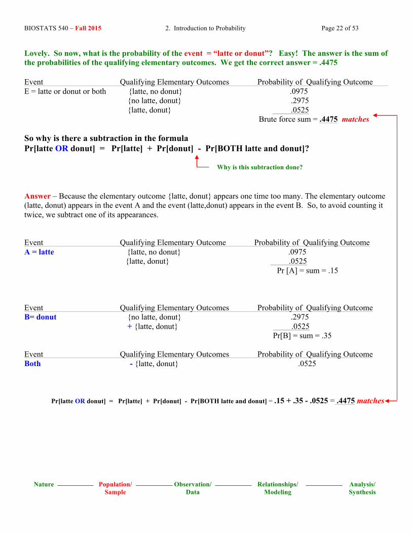
Lovely. So now, what is the probability of the event = “latte or donut”? Easy! The answer is the sum of the probabilities of the qualifying elementary outcomes. We get the correct answer = .4475 Event Qualifying Elementary Outcomes Probability of Qualifying Outcome E = latte or donut or both {latte, no donut} .0975 {no latte, donut} .2975 {latte, donut} .0525 Brute force sum = .4475 matches So why is there a subtraction in the formula Pr[latte OR donut] = Pr[latte] + Pr[donut] - Pr[BOTH latte and donut]? Why is this subtraction done? Answer – Because the elementary outcome {latte, donut} appears one time too many. The elementary outcome (latte, donut) appears in the event A and the event (latte,donut) appears in the event B. So, to avoid counting it twice, we subtract one of its appearances. Event Qualifying Elementary Outcome Probability of Qualifying Outcome A = latte {latte, no donut} .0975 {latte, donut} .0525 Pr [A] = sum = .15 Event Qualifying Elementary Outcomes Probability of Qualifying Outcome B= donut {no latte, donut} .2975 + {latte, donut} .0525 Pr[B] = sum = .35 Event Qualifying Elementary Outcomes Probability of Qualifying Outcome Both - {latte, donut} .0525 Pr[latte OR donut] = Pr[latte] + Pr[donut] - Pr[BOTH latte and donut] = .15 + .35 - .0525 = .4475 matches



Observation/ Data


Analysis/ Synthesis

The Addition Rule For two events, say A and B, the probability of an occurrence of either or both is written Pr [A ∪ B ] and is Pr [A ∪ B ] = Pr [ A ] + Pr [ B ] - Pr [ A and B ] Notice what happens to the addition rule if A and B are mutually exclusive! The subtraction of Pr [ A and B ] disappears because mutually exclusive events can never happen which means their probability is zero (Pr [ A and B ]=0) Pr [A ∪ B ] = Pr [ A ] + Pr [ B ]



Observation/ Data


Analysis/ Synthesis

7. The Multiplication Rule – The Basics When to Use the Multiplication Rule Tip – Think “and” Use the multiplication rule when you want to calculate the event that event “A” occurs and then event “B” occurs and then event “C” occurs and so on. The multiplication rule was introduced previously. See page 14, (4d. The Joint Probability of Independent Events). The Joint Probability of Two Independent Events is Obtained by Simple Multiplication Consider again the example from page 21 – Latte’s and Donuts ….– Wouldn’t you really rather have both a drink and something to eat? So now, instead of the event of “latte OR donut”, suppose we are interested in the event of “latte AND donut”. Yum. We use the multiplication rule to obtain the probability of both (much like we did on page 14 when we considered the outcome of two coin tosses). A = Outcome of latte at Starbucks. Pr[A] = .15 B = Outcome of donut at Dunkin Donuts Pr[B] = .35 Under the assumption that the outcomes at Starbucks and Dunkin Donuts are independent of one another, we can obtain our answer by simple multiplication: Pr[latte and donut] = Pr[latte] x Pr[donut] = (.15)(.35) = .0525 Introduction to Probability Trees Latte’s and Donuts, continued – We can construct a little probability tree that shows all the possibilities and their associated probabilities:

Probability .35 Donut (.15)(.35) = .0525 latte .65 No Donut (.15)(.65) = .0975 .15 .85 .35 Donut (.85)(.35) = .2975 No latte .65 No donut (.85)(.65) = .5525

Total = 1 or 100% Thus, we see that the Pr[latte and donut] = .0525 while Pr[latte and no donut] = .0975, and so on.



Observation/ Data


Analysis/ Synthesis

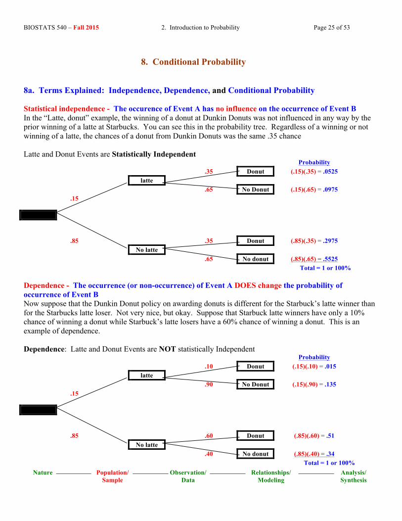
8. Conditional Probability 8a. Terms Explained: Independence, Dependence, and Conditional Probability Statistical independence - The occurence of Event A has no influence on the occurrence of Event B In the “Latte, donut” example, the winning of a donut at Dunkin Donuts was not influenced in any way by the prior winning of a latte at Starbucks. You can see this in the probability tree. Regardless of a winning or not winning of a latte, the chances of a donut from Dunkin Donuts was the same .35 chance Latte and Donut Events are Statistically Independent


Total = 1 or 100% Dependence - The occurrence (or non-occurrence) of Event A DOES change the probability of occurrence of Event B Now suppose that the Dunkin Donut policy on awarding donuts is different for the Starbuck’s latte winner than for the Starbucks latte loser. Not very nice, but okay. Suppose that Starbuck latte winners have only a 10% chance of winning a donut while Starbuck’s latte losers have a 60% chance of winning a donut. This is an example of dependence. Dependence: Latte and Donut Events are NOT statistically Independent


Total = 1 or 100%



Observation/ Data


Analysis/ Synthesis

More on Dependence - Two events are dependent if they are not independent. The probability of both occurring depends on the outcome of at least one of the two. Two events A and B are dependent if the probability of one event is related to the probability of the other event. Not independent! à If two events are dependent, then: P(A and B) ≠ P(A) P(B) It is still possible to calculate the joint probability of both “A” and “B occurring, P(A and B), but this requires a slightly different machinery. In particular, it requires knowing how to relate P(A and B) to what are called conditional probabilities. This is explained next. Conditional Probability Tip –Imagine you are in a situation where event “A” has occurred. Now you want an answer to the question “Given that A has occurred, now what is the probability that B will occur? The particulars of the event “A” having occurred changes the probability of the event “B” .

The conditional probability that event B occurs given that event A has occurred is denoted P(B|A) and is defined

P(B|A) = P(A and B)P(A)

= P(both A and B occur)P(A)

provided that P(A) ≠ 0.



Observation/ Data


Analysis/ Synthesis

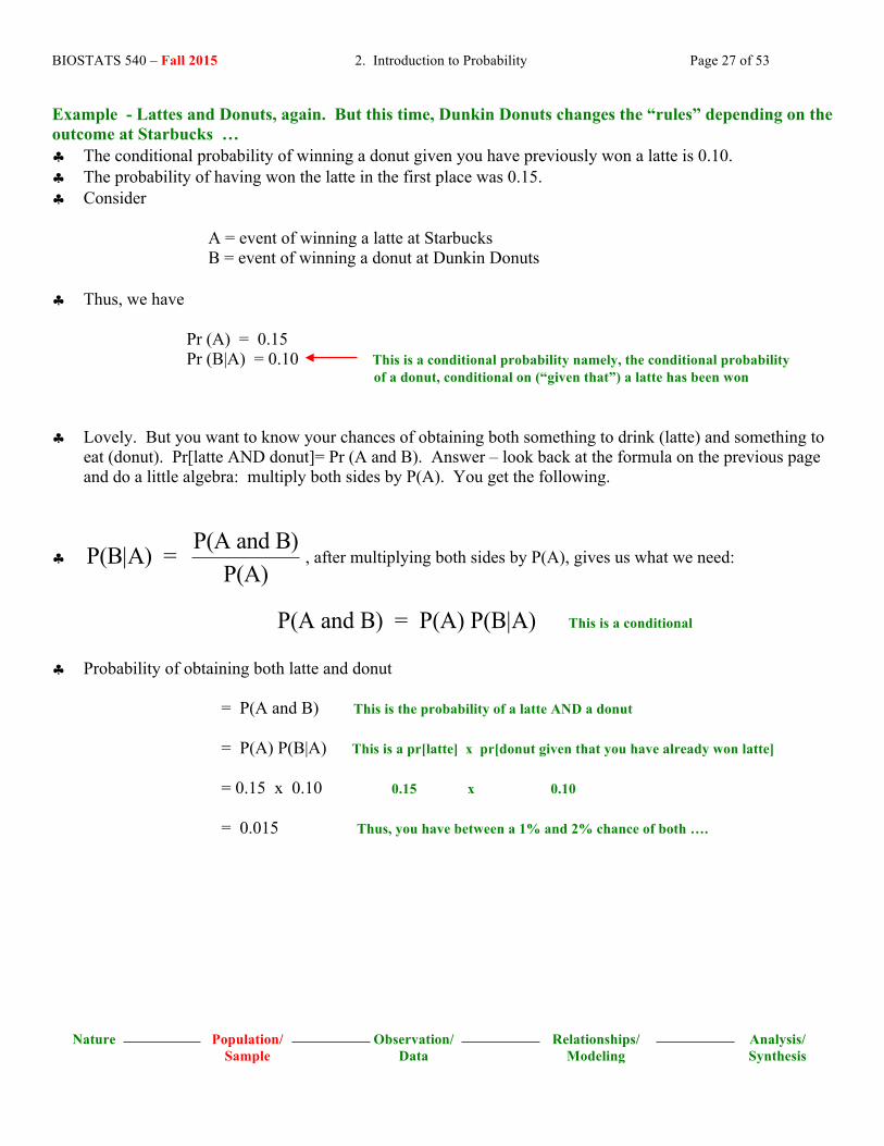
Example - Lattes and Donuts, again. But this time, Dunkin Donuts changes the “rules” depending on the outcome at Starbucks … ♣ The conditional probability of winning a donut given you have previously won a latte is 0.10. ♣ The probability of having won the latte in the first place was 0.15. ♣ Consider A = event of winning a latte at Starbucks B = event of winning a donut at Dunkin Donuts ♣ Thus, we have Pr (A) = 0.15 Pr (B|A) = 0.10 This is a conditional probability namely, the conditional probability of a donut, conditional on (“given that”) a latte has been won ♣ Lovely. But you want to know your chances of obtaining both something to drink (latte) and something to

eat (donut). Pr[latte AND donut]= Pr (A and B). Answer – look back at the formula on the previous page and do a little algebra: multiply both sides by P(A). You get the following.

♣ P(B|A) = P(A and B)P(A)

, after multiplying both sides by P(A), gives us what we need:

P(A and B) = P(A) P(B|A) This is a conditional

♣ Probability of obtaining both latte and donut = P(A and B) This is the probability of a latte AND a donut = P(A) P(B|A) This is a pr[latte] x pr[donut given that you have already won latte] = 0.15 x 0.10 0.15 x 0.10 = 0.015 Thus, you have between a 1% and 2% chance of both ….



Observation/ Data


Analysis/ Synthesis

8b. The Multiplication Rule – A Little More Advanced Tip – Think “and” Now that we have t he ideas of probability trees and conditional probability, we’re ready for the multiplication rule. Suppose you want to calculate the joint probability of event “A” occurs and then event “B” occurs and then event “C” occurs and so on.

Multiplication Rule

Pr[A and B and C] = Pr[A] • Pr[B|A] • Pr[C|B] provided (1) Pr[A] is not zero; and (2) the conditional probabilities are known; and (3) the conditional probabilities are not zero.

Example – Survival analysis Consider survival following an initial diagnosis of cancer. Suppose the one-year survival rate is .75. Suppose further that, given survival to one year, the probability of surviving to two years is .85. Suppose then that given survival to two years, the probability of surviving five years is then .95. What is the overall two survival rate? What is the overall five year survival rate? We can calculate the overall probabilities of surviving 2 and 5 years from just the probabilities given to us. The multiplication rule is used as follows:

Event of interest is probability of What we are given are conditional probabilities A = surviving 1 year Pr [ A ] = .75 B = surviving 2 years Pr [B | A ] = .85 C = surviving 5 years Pr [C | B] = .95



Observation/ Data


Analysis/ Synthesis

Overall 2-year survival = Pr [ B ] = Pr [ A ] Pr [ B| A ] Pr [ survival is 2 years or more ] = Pr[surviving 1 year] * Pr[surviving 2 years given survival to 1 year] * is the same as “times” = Pr[A] * Pr[B | A] = (.75) * (.85) = .6375 Overall 5-year survival = Pr [ C ] = Pr [ B ] Pr [ C | B ] = Pr [ A ] Pr [ B | A ] Pr [ C | B ] Pr [ survival is 5 years or more ] = Pr[surviving 1 year] * Pr[surviving 2 years given survival to 1 year] * Pr[surviving 5 yrs given 2 yrs] = Pr[A] * Pr[B | A] * Pr[C | B] = (.75) * (.85) * (.95) = .605625 In BIOSTATS 640, Intermediate Biostatistics, we will see that this is Kaplan-Meier estimation.



Observation/ Data


Analysis/ Synthesis

8c. TOOL - The Theorem of Total Probabilities Tip! Think chronology over time and map it out using a probability tree. The theorem of total probabilities is used when there is more than one path to a win and you want to calculate the overall probability of a win. Chronology over Time -

Step 1: First, choose one of two games to play: G1 or G2 G1 is chosen with probability = 0.85 G2 is chosen with probability = 0.15 (notice that probabilities sum to 1) Step 2: Now that you’ve chosen a game (“given that you choose a game, G1 or G2) : G1 yields “win” with conditional probability P(win|G1) = 0.01 G2 yields “win” with conditional probability P(win|G2) = 0.10

Probability Tree Tool -

.01 Conditional

Win (.85)(.01) = .0085

G1 chosen

.99 No win (.85)(.99) = .8415 .85

Choose Game

.15 .10 Conditional

Win (.15)(.10) = .015

G2 chosen

.90 No win (.15)(.90) = .135 What is the overall probability of a win, Pr(win)? Answer – ADD together the qualifying pathways! Pr(win) = Pr[G1 chosen] Pr[win|G1] + Pr[G2 chosen] Pr[win|G2]

= (.85) (.01) + (.15) (.10) = .0085 + 0.015 = 0.0235

This is the theorem of total probabilities.



Observation/ Data


Analysis/ Synthesis

Theorem of Total Probabilities

Suppose that a sample space S can be partitioned (carved up into bins) so that S is actually a union that looks like S = G G G1 2 K∪ ∪ ∪... If you are interested in the overall probability that an event “E” has occurred, this is calculated P[E] = P[G ]P[E|G ] + P[G P[E|G + ... + P[G P[E|G1 1 2 2 K K] ] ] ] pathway pathway pathway

provided the conditional probabilities are known.

Example – The lottery game just discussed. E = Event of a win

G1 = Game #1 G2 = Game #2

We’ll see this again in this course and also in BIOSTATS 640

♣ Diagnostic Testing ♣ Survival Analysis



Observation/ Data


Analysis/ Synthesis

8d. TOOL - Bayes Rule Tip! Bayes Rule is a clever “putting together” of the multiplication rule and the theorem of total probabilities.

1. Multiplication rule – This is our tool for computing a joint probability P(A and B) = P(A) P(B|A) = P(B) P(A|B)

2. Theorem of total probabilities – This provides us with a way of computing an overall pr[event] 1 1 2 2 K KP[E] = P[G ]P[E|G ] + P[G ]P[E|G ] + ... + P[G ]P[E|G ] Here is the rule. The next page is a “walk-through”

Bayes Rule

Suppose that a sample space S can be partitioned (carved up into bins) so that S is actually a union that looks like S = G G G1 2 K∪ ∪ ∪... If you are interested in calculating P(Gi |E), this is calculated

P[G |E] = P(E|G P(G

P[G ]P[E|G ] + P[G P[E|G + ... + P[G P[E|Gii i

1 1 2 2 K K

) )] ] ] ]

provided the conditional probabilities are known.



Observation/ Data


Analysis/ Synthesis

Example of Bayes Rule Calculation: “Given I have a positive screen, what are the chances that I have disease?” Source: http://yudkowsky.net/bayes/bayes.html This URL is reader friendly.

• Suppose it is known that the probability of a positive mammogram is 80% for women with breast cancer and is 9.6% for women without breast cancer.

• Suppose it is also known that the likelihood of breast cancer is 1% • If a women participating in screening is told she has a positive mammogram, what are the chances

that she has breast cancer disease? Let

• A = Event of breast cancer • X = Event of positive mammogram

à What we want to calculate is Probability (A | X) What we have as available information is

• Probability (X | A) = .80 Probability (A) = .01 • Probability (X | not A) = .096 Probability (not A) = .99

Here’s how the Bayes Rule solution works …

Pr(A and X)Pr( A | X ) = Pr (X)

by definition of conditional Probability

Pr(X | A) Pr(A)=

Pr(X) because we can re-write the numerator this way

Pr(X | A) Pr(A)=

Pr(X | A) Pr(A) + Pr(X | not A) Pr(not A) by thinking in steps in denominator

(.80) (.01)=

(.80) (.01) + (.096) (.99) = .078 , representing a 7.8% likelihood.



Observation/ Data


Analysis/ Synthesis

Alternative to Bayes Rule Formula for the Formula Haters: “Given I have a positive screen, what are the chances that I have disease?” Make a Tree of NUMBERS Using the Information about Prevalence and Test Results -

1st Disease

2nd Testing

80%

+ Test 800

Cancer 1,000

(1%)

20% - Test 200

100,000 Women

(99%)

9.6% + Test 9,504

Healthy 99,000

90.4% - Test 89,496

Time à

Counting Approach Solution From the “tree” of numbers,

Total # with positive test = 800 + 9,504 = 10, 304 # of individuals with positive test and cancer = 800 Pr[cancer given positive test]= Pr[cancer| + test]

# with cancer and +test= # with +test

800= 10,304

= .078

which matches the answer on page 33!



Observation/ Data


Analysis/ Synthesis

9. Probabilities in Practice – Screening Tests and Bayes Rule

In your epidemiology class, you are learning about:

• diagnostic testing (sensitivity, specificity, predictive value positive, predictive value negative); • disease occurrence (prevalence, incidence); and • measures of association for describing exposure-disease relationships (risk, odds, relative risk,

odds ratio).

Most of these have their origins in notions of conditional probability. 9a. Prevalence ("existing") The point prevalence of disease is the proportion of individuals in a population that has disease at a single point in time (point), regardless of the duration of time that the individual might have had the disease. In actuality, Prevalence is NOT a probability; it is a proportion. Example 1 - A study of sex and drug behaviors among gay men is being conducted in Boston, Massachusetts. At the time of enrollment, 30% of the study cohort were sero-positive for the HIV antibody. Rephrased, the point prevalence of HIV sero-positivity was 0.30 at baseline. 9b. Cumulative Incidence ("new") The cumulative incidence is a probability. The cumulative incidence of disease is the probability an individual who did not previously have disease will develop the disease over a specified time period. Example 2 - Consider again Example 1, the study of gay men and HIV sero-positivity. Suppose that, in the two years subsequent to enrollment, 8 of the 240 study subjects sero-converted. This represents a two-year cumulative incidence of 8/240 or 3.33%.



Observation/ Data


Analysis/ Synthesis

9c. Sensitivity, Specificity The ideas of sensitivity, specificity, predictive value of a positive test, and predictive value of a negative test are most easily understood using data in the form of a 2x2 table: Disease Status Breast Cancer Healthy

Test Positive 800 9, 504 10,304 Result Negative 200 89,496 89,696

1,000 99,000 100,000 Disease Status Present Absent

Test Positive a b a + b Result Negative c d c +d

a + c b +d a + b +c +d In this table, a total of (a+b+c+d) individuals are cross-classified according to their values on two variables: disease (present or absent) and test result (positive or negative). It is assumed that a positive test result is suggestive of the presence of disease. The counts have the following meanings: a = number of individuals who test positive AND have disease (=800) b = number of individuals who test positive AND do NOT have disease (=9,504) c = number of individuals who test negative AND have disease (=200) d = number of individuals who test negative AND do NOT have disease (=89,496) (a+b+c+d) = total number of individuals, regardless of test results or disease status (= 100,000) (b + d) = total number of individuals who do NOT have disease, regardless of their test outcomes (= 99,000) (a + c) = total number of individuals who DO have disease, regardless of their test outcomes (= 1,000) (a + b) = total number of individuals who have a POSITIVE test result, regardless of their disease status. (= 10,304) (c + d) = total number of individuals who have a NEGATIVE test result, regardless of their disease status. (= 89,696)



Observation/ Data


Analysis/ Synthesis

Sensitivity Sensitivity is a conditional probability. Among those persons who are known to have disease, what are the chances that the diagnostic test will correctly yield a positive result? Counting Solution: From the 2x2 table, we would estimate sensitivity using the counts “a” and “c”:

80.000,1800

c+aa=ysensitivit ==

Conditional Probability Solution:

( )( ) ( )

( )( ) ( )

sensitivity = Pr[+test|disease]

Pr["+test" AND "disease"] = Pr[disease]

a a+b+c+d =

a+c a+b+c+d

800 100,000 =

1,000 100,000

⎡ ⎤⎣ ⎦⎡ ⎤⎣ ⎦

⎡ ⎤⎣ ⎦⎡ ⎤⎣ ⎦

800 = 1,000

=.80

which matches the “counting” solution.



Observation/ Data


Analysis/ Synthesis

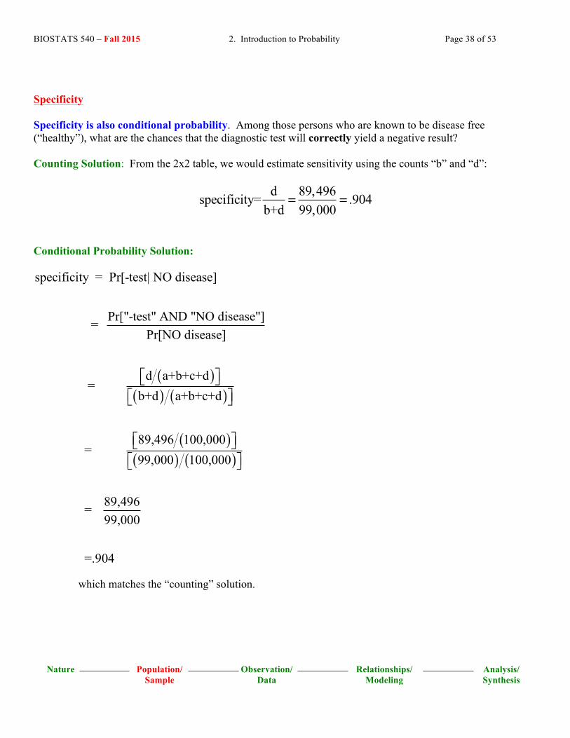
Specificity Specificity is also conditional probability. Among those persons who are known to be disease free (“healthy”), what are the chances that the diagnostic test will correctly yield a negative result? Counting Solution: From the 2x2 table, we would estimate sensitivity using the counts “b” and “d”:

d 89,496specificity= .904b+d 99,000

= =

Conditional Probability Solution:

( )( ) ( )

( )( )

specificity = Pr[-test| NO disease]

Pr["-test" AND "NO disease"] = Pr[NO disease]

d a+b+c+d =

b+d a+b+c+d

89,496 100,000 =

99,000

⎡ ⎤⎣ ⎦⎡ ⎤⎣ ⎦

⎡ ⎤⎣ ⎦( )100,000

89,496 = 99,000

=.904

⎡ ⎤⎣ ⎦

which matches the “counting” solution.



Observation/ Data


Analysis/ Synthesis

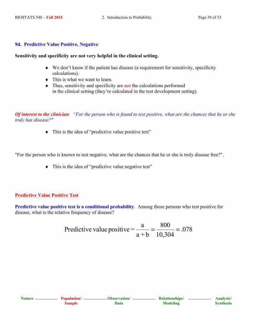
9d. Predictive Value Positive, Negative Sensitivity and specificity are not very helpful in the clinical setting.

♦ We don’t know if the patient has disease (a requirement for sensitivity, specificity calculations).

♦ This is what we want to learn. ♦ Thus, sensitivity and specificity are not the calculations performed

in the clinical setting (they’re calculated in the test development setting). Of interest to the clinician: “For the person who is found to test positive, what are the chances that he or she truly has disease?"

♦ This is the idea of “predictive value positive test” "For the person who is known to test negative, what are the chances that he or she is truly disease free?".

♦ This is the idea of “predictive value negative test” Predictive Value Positive Test Predictive value positive test is a conditional probability. Among those persons who test positive for disease, what is the relative frequency of disease?

078.304,10

800b+a

a = positive valuePredictive ==



Observation/ Data


Analysis/ Synthesis

Other Names for "Predictive Value Positive Test": * posttest probability of disease given a positive test * posterior probability of disease given a positive test Also of interest to the clinician: Will unnecessary care be given to a person who does not have the disease? Predictive Value Negative Test Predictive value positive test is a conditional probability. Among those persons who test negative for disease, what is the relative frequency of disease-free?

d 89,496Predictive value negative = .99

c+d 89,696= =

Other Names for "Predictive Value Negative Test": * post-test probability of NO disease given a negative test * posterior probability of NO disease given a negative test



Observation/ Data


Analysis/ Synthesis

10. Probabilities in Practice – Risk, Odds, Relative Risk, Odds Ratio Epidemiologists and public health researchers are often interested in exploring the relationship between a yes/no (dichotomous) exposure variable and a yes/no (dichotomous) disease outcome variable. Our 2x2 summary table is again useful. NOTE! Note that the rows now represent EXPOSURE status. We can do this because these numbers are hypothetical anyway. They are just for illustration. Disease Status Breast Cancer Healthy

Exposure Exposed 800 9, 504 10,304 Status Not exposed 200 89,496 89,696

1,000 99,000 100,000 Disease Status Present Absent

Test Exposed a b a + b Result Not exposed c d c +d

a + c b +d a + b +c +d a = number of exposed individuals who have disease (=800) b = number of exposed individuals who do NOT have disease (=9,504) c = number of NON exposed individuals who have disease (=200) d = number of NON exposed individuals who do NOT have disease (=89,496) (a+b+c+d) = total number of individuals, regardless of exposure or disease status (= 100,000) (b + d) = total number of individuals who do NOT have disease, regardless of exposure (= 99,000) (a + c) = total number of individuals who DO have disease, regardless of exposure (= 1,000) (a + b) = total number of individuals who are EXPOSED regardless of their disease status (= 10,304) (c + d) = total number of individuals who are NOT exposed regardless of their disease status. (= 89,696)



Observation/ Data


Analysis/ Synthesis

10a. Risk ("simple probability") Risk of disease, without referring to any additional information, is simply the probability of disease. An estimate of the probability or risk of disease is provided by the relative frequency:

( )

( )a+c 1,000Overall risk = .01

a+b+c+d 100,000= =

Typically, however, conditional risks are reported. For example, if it were of interest to estimate the risk of disease for persons with a positive exposure status, then attention would be restricted to the (a+b) persons positive on exposure. For these persons only, it seems reasonable to estimate the risk of disease by the relative frequency: The straightforward calculation of the risk of disease for the persons known to have a positive exposure status is:

a 800P(Disease | Exposed)= .078

(a+b) 10,304= =

Repeating the calculation using the definition of conditional probability yields the same answer.

( )( ) ( )

( )( ) ( )

Pr[ disease| + exposure]Pr["disease" AND "+ exposure"] =

Pr[+ exposure]a a+b+c+d

= a+b a+b+c+d

800 100,000 =

10,304 100,000

⎡ ⎤⎣ ⎦⎡ ⎤⎣ ⎦

⎡ ⎤⎣ ⎦⎡ ⎤⎣ ⎦

800 = 10,304

=.078

, which matches.



Observation/ Data


Analysis/ Synthesis

10b. Odds("comparison of two complementary (opposite) outcomes"): In words, the odds of an event "E" is the chances of the event occurring in comparison to the chances of the same event NOT occurring.

c

Pr(Event occurs) P(E) P(E)Odds = Pr(Event does NOT occur) 1 -P(E) (E )

= =

Example - Perhaps the most familiar example of odds is reflected in the expression "the odds of a fair coin landing heads is 50-50". This is nothing more than:

Odds(heads) = P(heads)P(heads

P(heads)P(tails)

.50

.50c )= =

For the exposure-disease data in the 2x2 table,

d)+(bc)+(a

d)+c+b+d)/(a+(bd)+c+b+c)/(a+(a

disease) P(NOP(disease)

)P(diseaseP(disease) = se)Odds(disea

c===

= 1,000

99,000= .0101

Odds(exposed) = P(exposed)P(exposed

P(exposed)P(NOT exposed)

(a + b) / (a + b + c + d)(c + d) / (a + b + c + d)

(a + b)(c + d)c )

= = =

10,304 .114989,696

= =



Observation/ Data


Analysis/ Synthesis

Conditional Odds. What if it is suspected that exposure has something to do with disease? In this setting, it might be more meaningful to report the odds of disease separately for persons who are exposed and persons who are not exposed. Now we’re in the realm of conditional odds.

Odds(disease | exposed) = Pr(disease|exposed)Pr(NO disease|exposed)

a / (a + b)b / (a + b)

ab

= =

800 .0849,504

= =

Odds(disease | NOT exposed) = Pr(disease|not exposed)Pr(NO disease|not exposed)

c / (c + d)d / (c + d)

cd

= =

200 .00289,496

= =

Similarly, one might calculate the odds of exposure separately for diseased persons and NON-diseased persons:

Odds(exposed | disease) = Pr(exposed|disease)Pr(NOT exposed|disease)

a / (a + c)c / (a + c)

ac

= =

800 4200

= =

Odds(exposed | NO disease) = Pr(exposed|NO disease)Pr(NOT exposed|NO disease)

b / (b + d)d / (b + d)

bd

= =

9,504 .106289,496

= =



Observation/ Data


Analysis/ Synthesis

11c. Relative Risk("comparison of two conditional probabilities") Various epidemiological studies (prevalence, cohort, case-control designs) give rise to data in the form of counts in a 2x2 table.

New! Example – Suppose we are interested in exploring the association between exposure and disease.

Disease Healthy Exposed a b a+b Not exposed c d c+d a+c b+d a+b+c+d Suppose now that we have (a+b+c+d) = 310 persons cross-classified by exposure and disease:

Disease Healthy Exposed 2 8 10 Not exposed 10 290 300 12 298 310 Relative Risk The relative risk is the ratio of the conditional probability of disease among the exposed to the conditional probability of disease among the non-exposed. Relative Risk: The ratio of two conditional probabilities

RR = a / (a + b)c / (c + d)

Example: In our 2x2 table, we have

a/(a+b) 2/10RR = 6c/(c+d) 10/300

= =



Observation/ Data


Analysis/ Synthesis

10d. Odds Ratio The odds ratio measure of association has some wonderful advantages, both biological and analytical. Recall first the meaning of an “odds”: Recall that if p = Probability[event] then Odds[Event] = p/(1-p) Let’s look at the odds that are possible in our 2x2 table:

Disease Healthy Exposed a b a+b Not exposed c d c+d a+c b+d a+b+c+d

Odds of disease among exposed = a/(a+b) a 2= = =.25b/(a+b) b 8⎡ ⎤⎢ ⎥⎣ ⎦

(“cohort” study)

Odds of disease among non exposed = c/(c+d) c 10= = =.0345d/(c+d) d 290⎡ ⎤⎢ ⎥⎣ ⎦

(“cohort”)

Odds of exposure among diseased = a/(a+c) a 2= = =.20c/(a+c) c 10⎡ ⎤⎢ ⎥⎣ ⎦

(“case-control”)

Odds of exposure among healthy = b/(b+d) b 8= = =.0276d/(b+d) d 290⎡ ⎤⎢ ⎥⎣ ⎦

(“case-control”)



Observation/ Data


Analysis/ Synthesis

Students of epidemiology learn the following great result! Odds ratio, OR In a cohort study: OR = Odds disease among exposed = a/b = ad Odds disease among non-exposed c/d bc In a case-control study: OR = Odds exposure among diseased = a/c = ad Odds exposure among healthy b/d bc Terrific! The OR is the same, regardless of the study design, cohort (prospective) or case-control (retrospective) Note: Come back to this later if this is too “epidemiological”! Example: In our 2x2 table, we have

OR = a *d

b*c=

2( ) 290( )8( ) 10( ) = 7.25



Observation/ Data


Analysis/ Synthesis

Thus, there are advantages of the Odds Ratio, OR. 1. Many exposure disease relationships are described better using ratio measures of association rather than difference measures of association. 2. ORcohort study = ORcase-control study

3. The OR is the appropriate measure of association in a case-control study.

- Note that it is not possible to estimate an incidence of disease in a retrospective study. This is because we select our study persons based on their disease status.

4. When the disease is rare, ORcase-control ≈ RR



Observation/ Data


Analysis/ Synthesis

Appendices 1. Some Elementary Laws of Probability

A. Definitions:

1) One sample point corresponds to each possible outcome of sampling. 2) The sample space (some texts do use term population) consists of all sample points. 3) A group of events is said to be exhaustive if their union is the entire sample space or population. Example - For the variable SEX, the outcomes "male" and "female" exhaust all possibilities. 4) Two events A and B are said to be mutually exclusive or disjoint if their intersection is the empty set. Example – One individual cannot be simultaneously "male" and "female". 5) Two events A and B are said to be complementary if they are both mutually exclusive and exhaustive. 6) The events E1, E2, ..., En are said to partition the sample space or population if: (i) Ei is contained in the sample space, and (ii) The event (Ei and Ej) = empty set for all i ≠ j; (iii) The event (E1 or E2 or ... or En) is the entire sample space or population.” In words: E1, E2, ..., En are said to partition the sample space if they are pairwise mutually exclusive and collectively exhaustive. Not sure of the meaning of “partitioning the sample space”? Imagine a whole pie that you cut into pieces. You’ve just partitioned the pie.



Observation/ Data


Analysis/ Synthesis

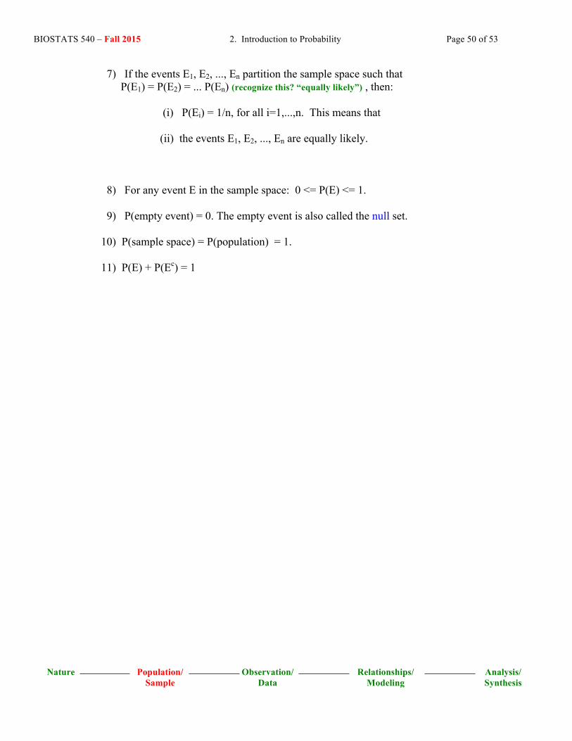
7) If the events E1, E2, ..., En partition the sample space such that P(E1) = P(E2) = ... P(En) (recognize this? “equally likely”) , then: (i) P(Ei) = 1/n, for all i=1,...,n. This means that (ii) the events E1, E2, ..., En are equally likely. 8) For any event E in the sample space: 0 <= P(E) <= 1. 9) P(empty event) = 0. The empty event is also called the null set. 10) P(sample space) = P(population) = 1. 11) P(E) + P(Ec) = 1



Observation/ Data


Analysis/ Synthesis

B. Addition of Probabilities - 1) If events A and B are mutually exclusive: (i) P(A or B) = P(A) + P(B) (ii) P(A and B) = 0 2) More generally: P(A or B) = P(A) + P(B) - P(A and B) 3) If events E1, ..., En are all pairwise mutually exclusive: P(E1 or ... or En) = P(E1) + ... + P(En)

C. Conditional Probabilities -

1) P(B|A) = P(A and B) / P(A) 2) If A and B are independent: P(B|A) = P(B) 3) If A and B are mutually exclusive: P(B|A) = 0 4) P(B|A) + P(Bc|A) = 1 5) If P(B|A) = P(B|Ac): Then the events A and B are independent

D. Theorem of Total Probabilities - Let E1, ..., Ek be mutually exclusive events that partition the sample space. The unconditional probability of the event A can then be written as a weighted average of the conditional probabilities of the event A given the Ei; i=1, ..., k: P(A) = P(A|E1)P(E1) + P(A|E2)P(E2) + ... + P(A|Ek)P(Ek) E. Bayes Rule - If the sample space is partitioned into k disjoint events E1, ..., Ek, then for any event A:

j jj

1 1 2 2 k k

P(A|E )P(E )P(E |A)=

P(A|E )P(E )+P(A|E )P(E )+...+P(A|E )P(E )



Observation/ Data


Analysis/ Synthesis

Appendices 2. Introduction to the Concept of Expected Value

We’ll talk about the concept of “expected value” again; this is an introduction. Suppose you stop at a convenience store on your way home and play the lottery. In your mind, you already have an idea of your chances of winning. That is, you have considered the question “what are the likely winnings?” Here is an illustrative example. Suppose the back of your lottery ticket tells you the following–

$1 is won with probability = 0.50 $5 is won with probability = 0.25 $10 is won with probability = 0.15 $25 is won with probability = 0.10

THEN “likely winning” = [$1](probability of a $1 ticket) + [$5](probability of a $5 ticket) + [$10](probability of a $10 ticket) + [$25](probability of a $25 ticket) =[$1](0.50) + [$5](0.25) +[$10](0.15) + [$25](0.10)

= $5.75

Do you notice that the dollar amount $5.75, even though it is called “most likely” is not actually a possible winning? What it represents then is a “long run average”.

Other names for this intuition are

♣ Expected winnings ♣ “Long range average” ♣ Statistical expectation!



Observation/ Data


Analysis/ Synthesis

Statistical Expectation for a Discrete Random Variable is the Same Idea.

For a discrete random variable X (e.g. winning in lottery) Having probability distribution as follows: Value of X, x = P[X = x] = $ 1 0.50 $ 5 0.25 $10 0.15 $25 0.10 The random variable X has statistical expectation E[X]=µ

µ = [x]P(X = x)all possible X=x

∑

Example – In the “likely winnings” example, the statistically expected winning is µ = $5.75

2. Introduction to Probability 2015 - UMass Amherstpeople.umass.edu/biep540w/pdf/2. Introduction to Probability 2015.pdf · BIOSTATS 540 – Fall 2015 2. Introduction to Probability

Documents