2. GOVERNING EQUATIONS 2.1 Two-phase Flow Regimes

2. GOVERNING EQUATIONS 2.1 Two-phase Flow Regimes The dynamics and evaporation of drops in a spray is influenced by the spray regime. Important regimes are summarized in Fig. 2.1. In a region where the spray drops occupy a significant fraction of the total volume of the two phase mixture, the spray is termed "thick" or dense. This regime is typically found in the region near the injector nozzle exit. At the other extreme, because practical sprays often diverge away from the nozzle, and the size of the drops is reduced due to evaporation and breakup, the spray drops far from the nozzle become isolated and have negligible mass and volume compared to that of the gas that has been set in motion by the spraying process. In this case, the spray is termed "very thin" or dilute and, although the drops continue to exchange mass, momentum and energy with the gas, the state of the gas is not altered appreciably by the exchange. The term "thin" spray has been used to describe the intermediate spray regime between the "very thin" and the "thick" regimes (O'Rourke, 1981).

Intact Churning Thick Thin Very thin

Computational cell

Fig. 2.1 Schematic representation of spray regimes for liquid injection from a single hole nozzle.

2.1

In the "very thin" spray regime, the gas flow field can be computed ignoring the volume occupied by the drops, and the drops can be tracked using the spray equation (Williams, 1985). In this case, the probable number of drops located in physical space between x and x+dx (i.e., the number of drops per unit volume), with drop radii in the range from r to r+dr, with drop velocities between v and v+dv and with temperatures between Td and Td+dTd at time t, is probable drop number/unit volume = f(x,r,v,Td,t) dr dv dTd Here the drop temperature is assumed to be uniform within the drop, and, since x and v are vector quantities, f is a function of 9 independent variables. The total fraction of the volume occupied by the gas is the gas-phase void (volume) fraction, θ, which is found by integrating the liquid volume over all of the different classes of drops (i.e., over all drop sizes, velocities and temperatures) θ = 1− (

43∫∫∫ π r3 f drdv dTd

Vol∫ )dVol / Vol (2.1)

In the "very thin" spray regime, isolated drop correlations can be used to calculate the exchanges between the drops and the gas and, since the drops are widely spaced, collisions and other interactions between drops can be ignored. In the "thin" spray regime, the drops occupy negligible volume but have significant mass compared to the gas, due to the large density ratio between the liquid and the gas. The drops influence the state of the gas, which, in turn, influences the rate of mass, momentum and energy exchange between other drops and the gas. For example, the wake produced by drops at the tip of a transient spray leads to a reduced relative velocity between the subsequent drops and the gas since these drops experience "drafting" forces. The reduced drag on the subsequent drops allows them to overtake the leading drops at the tip of the spray, and the process repeats. In the "thick" spray regime the drops occupy a significant volume fraction but are still recognizable as discrete drops or liquid

2.2

d

b

Fig. 2.2 Packing geometry for drops with diameter, d, spaced a distance, b, apart. "blobs" in a continuous phase. An appreciation for the values of θ that might represent a thick spray can be obtained by considering the geometrical packing problem shown in Fig. 2.2. It can be shown that for this cubic lattice arrangement (O'Rourke, 1981) θ = 1−

π3 3(1 + b / d)3

so when the drops are spaced one drop diameter apart θ = 0.92 (i.e., when b=d). When the drops touch each other the gas in the spaces between the drops represents a volume fraction θ = 0.395 (i.e., when b=0). These results suggest that a practical definition for beginning of the "thick" spray regime may be taken as θ < 0.9. In this case, drop-drop effects such as collisions and coalescence become extremely important. Exchange rates are then influenced by neighboring drops. A regime termed "churning flow" (O'Rourke, 1981) can be defined when the volume fraction of the liquid equals or exceeds that of the gas, and the liquid is no longer dispersed in a continuous gas phase. This regime occurs very close to (or even inside) the nozzle exit, in the region where the intact injected liquid first begins to breakup into a spray. In this case, equations of mass, momentum and energy conservation for compressible two-phase flows have been derived by considering the phases to be co-existing continua (e.g., Ishii, 1975). However,

2.3

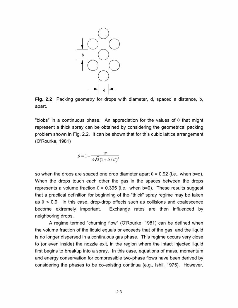
there is still considerable uncertainty about the form and the ranges of applicability of the coupling terms between the liquid and gas phases. Most current multidimensional spray simulations have adopted the "thin" or "very thin" spray assumptions, where the volume occupied by the dispersed phase is assumed to be small. As will be discussed next, the gas phase equations include source terms to account for exchange processes. This approach can be justified if the simulation starts some distance downstream of the nozzle exit, where the gas void fraction is large enough (e.g., θ > 0.9), or if the computational cells are relatively large, as is depicted in Fig. 2.1. "Thick" spray effects can be accounted for approximately, as is also described below. However, in order to formulate the exchange terms, it is first helpful to review the nature of conditions at a drop-gas interface. 2.2 Interface Conditions The interfacial region between fluids that do not mix behaves as if it were in a state of uniform tension due to molecular forces. In this region the physical properties differ noticeably from those in either bulk phase. Away from the critical point the interfacial layer is only a few molecules thick, and comparable to the wavelength of visible light. It is thus convenient to assume that the interface is a geometric surface across which there is a discontinuity in the pressure. As depicted in Fig. 2.3a, the surface can be characterized using two radii of curvature, R1 and R2, which are measured in perpendicular planes containing the local normal to the surface (positive if the center of curvature is in the liquid, as shown in Fig. 2.3a). If the surface is moved a distance dy in the direction of the normal to the surface, n, the area and volume of the liquid change by dA = d(S1 S2) = S1dS2 + S2dS1 and dV = dV1 = S1 S2 dy = - dV2, respectively. Analysis of the similar triangles in Fig. 2.3a shows that dS1/S1 = dy/R1, and dS2/S2 = dy/R2 or

dAdV

= (1R1

+1R 2

) = −∇ ⋅ n (2.2)

2.4

R

R

1

2

n

tgas

liquid Fig. 2.3a Details of interface region between liquid and the gas

Fig. 2.3b Infinitesimal control volume at liquid-gas interface

The discontinuity in pressure at the interface is supported by the surface tension force per unit area, where the surface tension, σ, is the excess free energy required to extend the surface area of the liquid by unit area at constant temperature. At equilibrium, thermodynamical arguments show that the Helmholtz free energy is a minimum, i.e., δF = − P1dV1 + P2dV2 + σ dA = 0 (2.3) where the terms involving pressure represent the work done in moving the surface. In the presence of evaporation, conservation of mass across the interface in Fig. 2.3b shows that Ý m = ρg (u − w) ⋅nd = ρl(v − w) ⋅ nd (2.4)

where Ým is the evaporative mass flux, ρ is the fluid density, w is the interface velocity, and u and v are the gas and liquid velocities, respectively, and nd is the unit outward normal pointing into the gas. Equations (2.2), (2.3) and (2.4) lead to an expression for the balance of normal forces on the fluid element shown in Fig. 2.3b, i.e., nd ⋅ (−PI + τ)l − nd ⋅(−P I + τ)g = σ∇ ⋅nd + Ý m (v − u) (2.5)

2.5

where P is the thermodynamic pressure, I is the unit dyadic, τ is the viscous stress tensor. The last term on the right-hand-side is the recoil force on the surface from vapor leaving the interface. As an example of the application of Eq. (2.5), consider a stationary spherical drop with radius R=R1=R2. The viscous stresses are zero in the absence of fluid motion and hence the pressure in the interior of the drop is higher than that of the surrounding gas pressure, i.e., Pl − Pg = 2σ / R .

A force balance at the interface also shows that the tangential stresses in the liquid and the gas must be equal, t (2.6) ⋅ τ l = t ⋅ τg

where, t is the tangent vector to the interface. Thus there is continuity in the shear stress at the interface, without which the fluid element shown in Fig. 2.3b would have an unbounded acceleration. 2.3 Gas Phase Equations The governing equations for the gas phase include equations for mass, momentum and energy conservation, supplemented by turbulence model equations. The interaction between the spray drops and the gas phase is accounted for by considering exchange functions. The present review is based on Williams (1985), O'Rourke (1981) and Amsden et al. (1985, 1989). The gas phase conservation equations are derived starting from an appropriate form of the Reynold's transport integral equation,

dΦdt

= ∂∂ t

ϕ ρ dvolVol( t )∫ + ϕ (ρV ⋅ ndA)

surf∫

= ∂∂t

(ϕ ρ )dvolVol( t )∫ + ϕ (ρV ⋅ ndA)

surf outer

∫ − ϕ (ρ{V − w} ⋅ nddA)surf d

∫ (2.7)

2.6

v

w

u

Fig. 2.4a Schematic diagram used for application of Reynold's transport integral equation (2.7) Equation 2.7 makes it possible to relate conservation principles that apply to systems (of fixed mass) to deformable volumes (of specified volume). For example, a school of small fish surrounded by a very coarse net, as depicted in Fig. 2.4a represents a system. The change in number of fish within the volume defined by the instantaneous shape of the net is related to the number of fish swimming through the holes in the net at velocity, v. Clearly, fish also escape through the net when the net is moved toward the fish with net velocity, w. These effects are represented by the terms on the right-hand-side of Eq. (2.7). In Eq. (2.7), V is the velocity of the fluid crossing the surfaces of the (time varying) control volume, Vol(t), and the surfaces of the control volume have been divided into two surfaces shown dotted in Fig. 2.4b. The "inner" surfaces, Surfd, are in contact with drops and the "outer" surface represents the outer surface of the entire control volume, Surfouter. dA is an element of the total surface. ϕ is a conserved intensive quantity, and Φ is the total (extensive) amount of that quantity in the system, as summarized in Table 2.1. In Fig. 2.4b, n = -nd is the unit normal pointing out of the gas.

2.7

Table 2.1 Summary of conservation variables for Eq. (2.7)

Quantity ϕ dΦ/dt Mass 1 0 Species Y chemical sources Momentum linear momentum per

unit mass u, v Sum of surface and body forces on c.v.

Energy internal plus kinetic energy, I +u2/2

Sum of heat and work transferred into c.v.

Volgn

u

dAVold

n d

dVolx

y

z

v

Fig. 2.4b Schematic diagram of control volume. Volg is the volume occupied by the gas (the surfaces of the volume are shown by the dashed lines, i.e., excluding the drops), Vold is the volume of the drops.

2.8

The term involving w in Eq. (2.7) arises from the application of Leibnitz' rule when the time derivative is moved inside the first integral on the right-hand-side, i.e., as the drops evaporate, the control surfaces at the drop-gas interfaces move at velocity, w. This causes the size of the control volume bounded by the area surfd to change with time. For simplicity it is assumed that there are no drops (or portions of drops) located on the outer surface of the control volume bounded by the area surfouter. The derivation of the conservation equations involves a limiting process where the spatial scale of the control volume in Eq. (2.7) is assumed to be large compared to the drop sizes, but small compared to the scale of change of gas phase properties. Figure 2.4b thus represents a small spatial region within a spray. The exchange terms result from evaluating the contributions from the surface area integrals at the interfaces between the dispersed drops and the gas in the control volume. The gas-phase volume fraction is θ(x,t) = ( dVol

Vo lg( t )∫ g) / Vol where Volg is the

volume occupied by the gas and the total volume is Vol = Volg + Vold (Vold is the volume occupied by the drops). Thus it follows that θ(x,t) = ( dVol

Vol ( t )∫ − dVold

Vold (t )∫ ) / Vol

which is the same as Eq. (2.1) since the first integral is equal to the total volume, and the second is the volume occupied by all the drops. In dense or thick sprays it is necessary to distinguish between the microscopic density of the gas, ρg (the gas mass per unit volume occupied by the gas) and the macroscopic gas mass-density, ρ = ρg θ (the gas mass per unit volume of mixture). In the absence of drops, the local gas-phase mass conservation equation is

{∂ρg

∂t+ ∇⋅(ρgu)

Vo lg∫ }dVo lg = 0 (2.8)

which follows from Eq. (2.7) when Gauss' theorem is applied to convert the surface integral to a volume integral. As shown in Table 2.1, ϕ = 1, and dΦ/dt=0, since the total mass in the system is constant. Also V = u, where u is the velocity of the gas leaving the "outer" surface of the control volume. Since the volume was chosen

2.9

arbitrarily, the term in braces in Eq. (2.8) must be zero, and this is the differential form of the mass conservation equation for the (microscopic) gas density. When spray drops are present and Eq. (2.7) is integrated over the gas (see Fig. 2.4b), the differential form of Eq. (2.8) becomes

{∂ρ∂t

+ ∇ ⋅(ρu)}Vol∫ dVol = − ρg

Surfd

∫ (u − w) ⋅n ddA (2.9)

The second term on the left-hand-side of Eq. (2.9) represents the (gas) mass leaving the "outer" surface of the control volume at the gas velocity, u. The integral on the right-hand-side represents the source/sink of gas mass due to evaporation/condensation from the drops, as was also discussed in Eq. (2.4). Applying Eq. (2.7) to an individual drop, gives the rate of change of liquid mass (e.g., due to evaporation) as

∂∂ t

(43 π r 3ρl) = ρl

Surfd

∫ (w − v) ⋅ nd dA (2.10)

where ρl is the liquid density, v is the drop velocity and the integration is over the surface of the drop. From mass conservation (see Eq. (2.4), it follows that the right hand sides of Eqs. (2.9) and (2.10) must be equal, and when Eq. (2.10) is summed over all of the drops, and the liquid density is assumed to be constant, Eq. (2.9) becomes

∂ρ∂t

+ ∇ ⋅(ρu) = − ρl 4πr 2∫∫∫ R f drdv dTd (2.11)

This is the final form of the mass conservation equation. Expressions for the time rate of change of drop radius, R = dr/dt, will be considered in Section 4.5.

2.10

Similar derivations are followed for the momentum and the energy equations. For example, for a single drop, linear momentum conservation gives

∂∂ t

(43 π r 3ρlv) = [ρl

Surfd

∫ v(w − v) ⋅n d − pdn d + τd ⋅ nd ]dA

or, using Eq. (2.5) 4

3 πr 3ρlF = [ρg(Surfd

∫ u − v)(u − w) ⋅n − Pgn + τg ⋅ n+ σ∇⋅ n]dA (2.12)

where the acceleration of the drops is F= dv/dt, and the right-hand-side of Eq. (2.12) follows from the interface condition, Eq. (2.4). When Eq. (2.7) is integrated over the gas volume, Volg, with ϕ=u, it can be shown that the integral in Eq. (2.12) appears as the source term on the right hand side of the equation (O'Rourke, 1981). The term involving the surface tension is zero if the surface tension is constant over the surface of the drop, and the thrust imparted to the drop (first term on the right-hand-side) is zero if the evaporation is symmetric. Similarly, energy conservation considerations for a single drop give rise to terms that account for the energy required to heat the drop and the work associated with the normal stresses plus heat transfer. These source terms are discussed further in the next section. The mass conservation equation can be generalized for a mixture of reacting gases. The equation for species m has source terms arising from the vaporizing spray and chemical reactions, i.e.,

∂ρm∂t

+ ∇ ⋅ ρm u = ∇⋅ ρD∇ ρmρ + ρm

c + ρsδm1 (2.13)

where ρm is the mass density of species m, ρ is the total mass density, i.e., ρm

m∑ , D

is the (molecular plus turbulent) diffusion coefficient of Fick's Law, and ρmc is the

source term due to chemical reactions (i.e., the dΦ/dt term in Table 2.1). Species 1 corresponds to the fuel and δ is the Kronecker delta function and ρsδm1 corresponds to the source term on the right-hand-side of Eq. (2.11). As usual, pressure gradient and Soret and Dufour diffusion effects are neglected (Williams, 1985). The momentum equation for the fluid mixture becomes

2.11

∂ρu∂ t

+ ∇⋅ (ρuu) = −∇p − ∇( 23 ρk) + ∇τ + Fs + ρg (2.14)

where P is the fluid pressure, k is the turbulent kinetic energy, τ is the (laminar plus turbulent) viscous stress tensor in Newtonian form, τ = ρD{[∇u + ∇uT ] − 2

3 ∇⋅ uI}

where I is a unit dyadic. Fs is the rate of momentum gain per unit volume due to the spray, as discussed in Eq. (2.12), and g is the body force which is assumed to be constant. The internal energy equation is

∂ρI∂t

+ ∇ ⋅ ρuI = -P∇⋅u - ∇⋅J + ρε + Qc + Qs

(2.15) where I is the specific internal energy, exclusive of chemical energy, J is the heat flux vector including turbulent heat conduction and enthalpy diffusion effects, i.e., J = −λ∇T − ρD hm

m∑ ∇(ρm / ρ)

where λ is the thermal conductivity, T is the gas temperature, hm is the specific enthalpy of species m, and Q

c and Q

s are the source terms due to the chemical heat

release and spray interactions. The turbulent transport of mass, momentum and energy is controlled by diffusion coefficients that are modeled as D = Cµ k2 / ε (2.16)

with appropriate forms for the turbulence Prandlt and Schmidt numbers. Cµ = 0.09 is a constant and k, is the turbulent kinetic energy k and, ε, is its dissipation rate which are typically modeled by the k-ε turbulence model using transport equations as follows,

∂ρk∂t

+ ∇⋅ (ρuk) = − 23 ρ k∇⋅ u + τ ⋅ u + ∇⋅ (

µPr k

)∇k⎡

⎣ ⎢ ⎤

⎦ ⎥ −ρε + Ý W s (2.17)

2.12

∂ρε∂t

+ ∇ ⋅ ρuε = - 23

Cε1 - Cε3 ρε∇⋅ u + ∇⋅ µPrε

∇ε

+ ε

k Cε1τ :∇u - Cε2ρε + CsW

s

(2.18) These are standard k-ε equations with some added terms. The source term - 2

3Cε1 - Cε3 ρε∇⋅u accounts for length scale changes when there is velocity

dilatation. The terms involving the shear stress, τ, represent turbulence production. Source terms involving the quantity W s arise due to interactions with the spray. The model constants use the values from the standard k-ε model, i.e., Cε1=1.44, Cε2=1.92, Cε3=-1.0, Prk=1.0, Prε=1.3, and Cs=1.5 as suggested by Amsden et al. (1989). Other turbulence models have been proposed for spray modeling, including Reynolds stress models, subgrid scale (SGS) turbulence model (large eddy simulation models) and, recently, the RNG (Renormalized Group theory) modification of the k-ε model (Yakot et al., 1992). To complete the governing equations, state equations are required. These are usually assumed to be those of an ideal gas mixture, e.g., p = RT ρm

m∑ / Wm (2.19)

where R is the universal gas constant and Wm is the molecular weight of species m. The thermodynamic quantities such as the specific internal energy, Im(T), specific heat cpm(T) and enthalpy, hm(T), are taken from the JANAF tables (Stull and Prophet, 1971). In addition, boundary conditions which depend on the specific application are required for the flow variables, e.g., periodic, or inflow/outflow boundaries, rigid walls with free slip, no-slip, or turbulent law-of-the-wall conditions. Temperature boundary condition options are adiabatic walls and fixed temperature walls. In calculations of turbulent flow, boundary conditions for turbulent kinetic energy k and its dissipation rate ε are taken to be

∇k⋅n = 0 and ε = Cµε k

3/2y (2.20)

2.13

where k and ε are evaluated a distance y from the wall and Cµε=0.38. The effect of compressibility on the turbulence has also been accounted for by using a transformed distance in Eq. (2.20) and in the turbulent law-of-the-wall dy' = ρ / ρ0 dy , where ρ0 is a reference density as described by Reitz (1991b). 2.4 Spray Equation and Exchange Terms The spray equation of (Williams, 1985), describes the evolution of the droplet distribution function, f.. In the KIVA model, f has eleven independent variables including three droplet position coordinates x, three velocity components v, the drop radius coordinate r, the drop temperature Td (assumed to be uniform within the drop), and the drop's distortion from sphericity y, the time rate of change dy/dt=y, and time t. Therefore, f(x, v, r, Td, y,y,t) dr dv dTd dy dy (2.21) is the probable number of droplets per unit volume at position x and time t with velocities in the interval (v, v+dv), radii in the interval (r, r+dr), temperatures in the interval (Td, Td+dTd) and displacement parameters in the intervals (y, y+dy) and (y, y+dy). The time evolution of f is obtained by solving a form of the spray equation,

∂f∂t

+ ∇x ⋅ fv + ∇v ⋅ fF + ∂∂r

(fR ) + ∂∂Td

fTd + ∂∂y

fy + ∂∂y

fy = fcoll + fbu (2.22)

In the above equation, the quantities F, R, Td, and y are the time rates of changes, following an individual drop, of its velocity, radius, temperature, and oscillation velocity y. The terms fcoll and fbu are the sources due to droplet collisions and breakup. All these spray droplet parameters must be provided by the spray model. By solving the spray equation, the exchange functions ρs, Fs, Q

s, and W s can

be obtained for the use in Eqs. (2.11), (2.13-15) and (2.17-18). These are obtained by summing the rate of change of mass, momentum, and energy of all droplets at position x and time t.

ρs = - fρd4πr2R dv dr dTd dy dy

(2.23)

2.14

Fs = - fρd 4/3 πr3F ' + 4πr2Rv dv dr dTd dy dy

(2.24)

Qs = - fρd 4πr2R Il+1

2v-u 2 + 4/3 πr3 clTd + F '⋅ v-u-u'

dv dr dTd dy dy (2.25)

W s = - fρd 4/3 πr3F '⋅u' dv dr dTd dy dy

(2.26) where F'=F - g, (v-u) is the relative velocity between the drop and the gas, u' is the gas-phase turbulence velocity (assumed to be normally distributed with a variance of

23k), Il and cl are the internal energy and specific heat of liquid drops,

respectively. Physically, Ý ρ s is the rate of mass evaporation from the drops, Fs is the force transmitted to the gas through droplet drag, body forces and momentum exchange due to evaporation, Ý Q s is the energy transmitted to the gas by evaporation, by heat transfer into the drop and by work due to turbulent fluctuations, and W s is the negative of the rate at which the turbulent eddies are doing work in dispersing the droplets. Through these exchange functions, interactions between spray droplets and gas phase are then accounted for.

2.15

2.5 Classification of Models Two main classes of models are used in spray modeling that differ in assumptions used to simplify the governing equations. In the limit of very small drops it can be safely assumed that the spray drops are in dynamic and thermodynamic equilibrium with the gas. At each point in the flow the drops have the same velocity and temperature as that of the gas, and the phases are in equilibrium. 'Slip' between the phases is neglected and the models are referred to as Locally Homogeneous Flow models (LHF). In this case the spray is "very dilute", the spray equation is not needed, and the source terms in the gas equations due to the spray are neglected (e.g., Dodge, 1995 - Appendix A). The main modification to the gas-phase equations involves the introduction of a mixture density, ρ, which includes the partial density of species both in the liquid and gas phases. For example ρ = (Y fl / ρ fl + Y fg / ρ fg + YA / ρ A)−1

where Y is the species mass fraction, and the subscripts A refers to the "air" or inert species and, f, l, g, refer to the "fuel" species in its liquid and gaseous phases, respectively. For vaporization problems the local fuel vapor mass fraction, Yfg, is found from the vapor pressure, Pfg, using equilibrium equations such as the Clausius Clapyron equation, LogPfg = A − B / T , where the total pressure, P = PA +

Pfg (the liquid phase is assumed to occupy negligible volume and thus does not to contribute to the total pressure), T is the local (saturation) temperature and A and B are constants that depend on the fuel type. Applications of LHF models are discussed in detail by Faeth (1983). The other major class of models are the Two-Phase-Flow or Separated-Flow (SF) models which are considered in detail in the following sections. These are the most general models since they account for effects due to finite rates of mass, momentum and energy exchange between the gas and liquid phases and all of the terms are retained in the liquid and gas conservation equations. As discussed previously, due to computer storage and run-time limitations it is not possible to accurately model the details of flows around individual drops. Thus, the exchange processes between the phases are modeled using semi-empirical correlations, as will be discussed in Chapter 4.

2.16

2.6 Numerical Implementation The gas-phase field equations are typically solved using an Eulerian finite difference or finite volume approach. Good introductions to numerical methods for CFD (Computational Fluid Dynamics) are given by Roache (1976) or Warsi (1993). The three-dimensional computational domain is divided into a number of small cells that are hexahedrons, as shown in Fig. 2.5, or in some applications, into cells that are tetrahedrons. Typical computational meshes are either structured or unstructured (i.e., the cells are joined regularly or in an 'arbitrary' manner to fill any volume, respectively), and the cells can distort in a prescribed time-varying fashion to accommodate boundary motion. An example is the 'Arbitrary Lagrangian-Eulerian' method of the KIVA code (Amsden et al., 1989) in which the cell vertices can be moved with the fluid velocity (Lagrangian - with no convection across cell boundaries), or remain

Fig. 2.5 Typical numerical mesh for 3-D spray computations fixed (Eulerian), or be moved following some user prescribed motion. In KIVA the mesh need not be orthogonal and the volume of each cell is effectively the control

2.17

volume of Eq. (2.7). In some codes sliding motion between adjacent mesh regions is allowed which is useful for treating problems involving rotational movements between parts, such as in rotating machinery (e.g., STAR-CD, 1994). Dynamic addition and removal of cells is desirable, to facilitate control over mesh resolution and mesh distortion in moving boundary problems. In finite volume codes, the divergence terms in the equations are transformed to surface integrals using the divergence theorem, thus ensuring local mass, momentum and energy conservation. Accurate solutions usually require that the convective terms in the governing equations be represented with second order difference schemes. However, in practice, considerations of numerical stability usually require the use of schemes that are effectively less than second order accurate. For a transient flow computation, the transient solution is marched out in a sequence of timesteps. The time differencing can be explicit or implicit (advanced time level data is not needed or is needed, respectively). The maximum value of the numerical timestep is usually restricted by the sound speed or convective (CFL) or diffusive constraints in explicit codes, and numerical instabilities can result if these restrictions are violated. Implicit codes are generally more robust, but can be less accurate if the time steps are too large. The so-called SIMPLE algorithm (Semi-Implicit Pressure Linked Equations (Patankar, 1980) is often used solve the momentum and continuity equations for compressible flow applications. In this case, the pressure field is obtained by solving a modified Poisson equation, and the solution is iterated until the continuity equation is satisfied to within a specified tolerance. Numerical accuracy is also influenced by grid resolution, and can be assessed by repeating the computations on successively finer grids. Gonzalez et al. (1992) studied diesel combustion in a Cummins diesel engine using the KIVA code and computational domain shown in Fig. 2.6 which had 24x12x18 cells with non-uniform azimuthal spacing).

2.18

Fig. 2.6 Perspective view of computational grid used for Cummins engine diesel combustion studies (Gonzalez et al., 1992).

Fig. 2.7 Plan view of sprays showing effect of grid resolution on predicted spray penetration. Top: Coarse grid of 25x6x18 cells. Bottom: Finer grid of 24x12x18 cells with non-uniform azimuthal spacing (Gonzalez et al., 1992).

2.19

To save computer time, 45 degree sector symmetry was assumed and the computations only considered one of the 8 spray nozzles. Computational experiments showed that the results were most sensitive to the azimuthal mesh spacing. This is demonstrated in Fig. 2.7 which compares predictions of spray penetration at TDC for a grid of 25x6x18 cells (equal spaced in the azimuthal direction) and a grid with non-uniform azimuthal spacing with increased resolution in the vicinity of the spray. The spray drop locations are indicated by the circles. The sensitivity of the spray penetration to the azimuthal mesh spacing is explained by the fact that the largest gradients in the flow are across the spray cross-section. The numerical details also influence combustion predictions. Predicted engine cylinder pressures made using meshes with uniform azimuthal mesh spacings of 7.5, 2.25, 1.8 and 1 degrees are shown in Fig. 2.8. These computations were made using 25x18 cells in the radial and axial directions, respectively.

3000

4000

5000

6000

7000

-20 -15 -10 -5 0 5 10

Pre

ssur

e (k

Pa)

Crank Angle (degrees)

1.01.8

2.257.5

Fig. 2.8 The effect of grid resolution on predicted cylinder pressure using grids with azimuthal mesh spacings of 7.5, 2.25, 1.8 and 1.0 degrees (equally spaced).

2.20

Table 2.2 Error estimates for the peak cylinder pressure as a function of azimuthal mesh spacing, ∆φ (Gonzalez et al., 1992). grid ∆φ max.

pressure (kPa)

error (%)

cpu time (hour)

∆φ=0 7233 (est.)

- -

1° 6875 4.95 14.5 1.8° 6589 8.89 6.5 2.25° 6249 13.6 3.5 7.5° 5619 22.4 0.3 It can be seen that finer grid resolution gives higher cylinder pressures (faster combustion). The magnitude of the numerical error in the peak pressure can be estimated using the Richardson extrapolation technique where the results of two computations made on successively finer meshes with spacings ∆φ1 and ∆φ2 are used to estimate the 'exact' solution, P(0), from:

P(0) = ∆φ2 P(∆φ1) - ∆φ1 P(∆φ2) / (∆φ2-∆φ1)

As can be seen from Table 2.2, the convergence is quite slow, and very fine mesh resolution is needed to get accurate results. The cpu time in Table 2.2 is the time spent during the combustion period from 18 crank angle degrees before top dead center to 8 degrees after top dead center. The results show that to maintain reasonable accuracy while avoiding excessive computer time, an azimuthal grid size of less than about 2° is a good compromise.

2.21

The spray equation, Eq. (2.22), has been solved by some researchers using an Eulerian finite difference method (e.g., Gupta and Bracco, 1978). However, this method has been found to be impractical since each independent variable has to be discretized on a grid, and with the 11 independent variables of Eq. (2.22) the computer storage required becomes excessive (e.g., with a coarse mesh of 10 mesh points in each dimension, 1011 grid points would be needed). A practical solution technique is the Lagrangian Monte Carlo approach proposed by Dukowicz, 1980, and implemented in the KIVA code (Amsden et al., 1989). Here the paths of stochastic parcels of drops are followed in physical, velocity, radius and temperature space (together with the drop distortion parameters). Mathematically, the spray Eq. (2.22) is a hyperbolic equation, and the paths represent characteristics in the solution space. As depicted in Fig. 2.9, a drop is moved to its new location in physical space after a time interval, dt following

u

v

t t+dt

u'

l

Fig. 2.9 Schematic diagram of spray drop history in a computational cell during time dt.

2.22

dxdt

= v (2.27)

The drop velocity vector is determined from dv

dt= F (2.28)

where the force per unit mass, F, on the drop (see Eq. 2.24) depends on drop drag and body forces. As will be discussed in Section 4.2, the drop drag depends on the gas mean velocity, u (which is defined at the vertices of the computational cell shown in Fig. 2.6), and on the gas turbulence velocity, u', and the turbulence eddy length scale, l, and the drop size, r. For a vaporizing spray, the change in drop size with time is determined from dr

dt= R (2.29)

where the quantity, R, is found from vaporization rate correlations, as will be discussed in Section 4.5. The drop size is also influenced by drop breakup and drop collision and coalescence, to be discussed in Sections 4.1 and 4.4. From Eq. (2.22) it is seen that these effects lead to a change in the number of drops in a particular size class, and to the appearance (or disappearance) of drops from the computation, which can be expressed as df = ( Ý f coll + Ý f bu )dt (2.30)

In the stochastic particle model of Dukowicz (1980), each parcel represents a number of identical drops, each with the same values of drop velocity, drop radius, drop temperature, and drop distortion and turbulent eddy parameters. The collection of parcels in the computational domain represents the spray drop number distribution and, since only discrete values of the independent variables are represented in the computation, as the number of parcels is increased, the statistics are improved. To start a spray computation, drop parcels are introduced at a specified rate at the injector location with specified drop sizes, velocities and temperatures, etc. (i.e., specified atomization characteristics). The injection velocities are

2.23

usually determined from measurements of the injector nozzle mass flow rate, or from the equation U = CD 2∆P ρl (2.27)

where CD is the nozzle discharge coefficient (determined experimentally or assumed) and ∆P is the injection pressure, Pl-Pg. The injected drops undergo further breakup and penetrate into the gas while interacting with each other (through collisions and coalescences) and with the gas (through the exchange terms). The mass, momentum and energy exchange is preferably treated implicitly to avoid small numerical timesteps. Submodels for these processes are discussed in more detail below. An alternative spray modeling approach called the PSI Cell (Particle-Source-in-Cell) model was proposed by Crowe et al. (1977). This technique is most suited for steady-state spray computations and is currently in use in many commercially available spray codes. The procedure begins by solving the gas flow field assuming that no particles are present in the flow. Particle trajectories, and the mass and temperature history on each trajectory are then computed. The particle properties are used to calculate the mass, momentum and energy source terms for the gas in each cell traversed by the particles. The gas flow field is then recalculated, incorporating these source terms. New trajectories are then computed, the source terms reevaluated, and the process continues until the flow field converges. The basic difference between the PSI and the stochastic parcel approach of Dukowicz (1980) is that in Dukowicz' method the drop motion equations are solved as functions of time, and the drop-gas coupling is non-iterative. The PSI Cell method is not well suited for modeling particle dispersion effects in turbulent sprays, since these flows are inherently unsteady (see Section 4.3).

2.24