Dick, H.J.B., Natland, J.H., Miller, D.J., et al., 1999 Proceedings of the Ocean Drilling Program, Initial Reports Volume 176 2. EXPLANATORY NOTES 1 Shipboard Scientific Party 2 INTRODUCTION In this chapter, we have assembled information that will help the reader understand the basis for our preliminary conclusions and help the interested investigator select samples for further analysis. This information concerns only shipboard operations and analyses described in the site reports in the Initial Reports volume of the Leg 176 Proceedings of the Ocean Drilling Program. Methods used by various inves- tigators for shore-based analyses of Leg 176 data will be described in the individual scientific contributions published in the Scientific Results vol- ume and in publications in various professional journals. Authorship of Site Chapter The separate sections of the site chapter were written by the follow- ing shipboard scientists (authors are listed in alphabetical order, no seniority is implied): Leg Summary: Dick, Natland Operations: Dick, Miller, Natland, Storms Igneous Petrology: Holm, Le Roux, Maeda, Meyer, Naslund, Natland, Niu, Snow Metamorphic Petrology: Alt, Bach, Bideau, Kelley, Robinson Geochemistry: Hertogen Structural Geology: Hirth, Ildefonse, John, Trimby, Yoshinobu Paleomagnetism: Gee, Kikawa, Worm Physical Properties: Kingdon, Stephen Downhole Logging: Haggas, Iturrino, Kingdon, Stephen, Worm Shore-based Logging: Bartetzko Visual Core Description: Shipboard Scientific Party 1 Examples of how to reference the whole or part of this volume. 2 Shipboard Scientific Party addresses. Ms 176IR-102

Welcome message from author
This document is posted to help you gain knowledge. Please leave a comment to let me know what you think about it! Share it to your friends and learn new things together.
Transcript

Dick, H.J.B., Natland, J.H., Miller, D.J., et al., 1999Proceedings of the Ocean Drilling Program, Initial Reports Volume 176
2. EXPLANATORY NOTES1
Shipboard Scientific Party2
INTRODUCTION
In this chapter, we have assembled information that will help thereader understand the basis for our preliminary conclusions and helpthe interested investigator select samples for further analysis. Thisinformation concerns only shipboard operations and analysesdescribed in the site reports in the Initial Reports volume of the Leg 176Proceedings of the Ocean Drilling Program. Methods used by various inves-tigators for shore-based analyses of Leg 176 data will be described in theindividual scientific contributions published in the Scientific Results vol-ume and in publications in various professional journals.
Authorship of Site Chapter
The separate sections of the site chapter were written by the follow-ing shipboard scientists (authors are listed in alphabetical order, noseniority is implied):
Leg Summary: Dick, NatlandOperations: Dick, Miller, Natland, StormsIgneous Petrology: Holm, Le Roux, Maeda, Meyer, Naslund, Natland,
Niu, SnowMetamorphic Petrology: Alt, Bach, Bideau, Kelley, RobinsonGeochemistry: HertogenStructural Geology: Hirth, Ildefonse, John, Trimby, YoshinobuPaleomagnetism: Gee, Kikawa, WormPhysical Properties: Kingdon, StephenDownhole Logging: Haggas, Iturrino, Kingdon, Stephen, WormShore-based Logging: BartetzkoVisual Core Description: Shipboard Scientific Party
1Examples of how to reference the whole or part of this volume.2Shipboard Scientific Party addresses.
Ms 176IR-102
SHIPBOARD SCIENTIFIC PARTYCHAPTER 2, EXPLANATORY NOTES 2
Numbering of Sites, Holes, Cores, and Samples
Drilling sites are numbered consecutively from the first site drilled bythe Glomar Challenger in 1968. A site refers to one or more holes drilledwhile the ship was positioned over a single acoustic beacon. Multipleholes are often drilled at a single site by pulling the drill pipe above theseafloor (out of the hole), offsetting the ship some distance from theprevious hole (without deploying a new acoustic beacon), and drillinganother hole.
For all Ocean Drilling Program (ODP) drill sites, a letter suffix distin-guishes each hole drilled at a single site. The first hole at a given site isassigned the suffix A, the second hole is designated with the same sitenumber and assigned suffix B, and so on. Note that this procedure dif-fers slightly from that used by the Deep Sea Drilling Project (DSDP; Sites1–624) but prevents ambiguity between site- and hole-number designa-tions. These suffixes are assigned regardless of recovery, as long as pene-tration takes place. Distinguishing among holes drilled at a site isimportant, because recovered rocks from different holes, particularlywhen recovery is less than 100%, are likely to represent different inter-vals in the cored section.
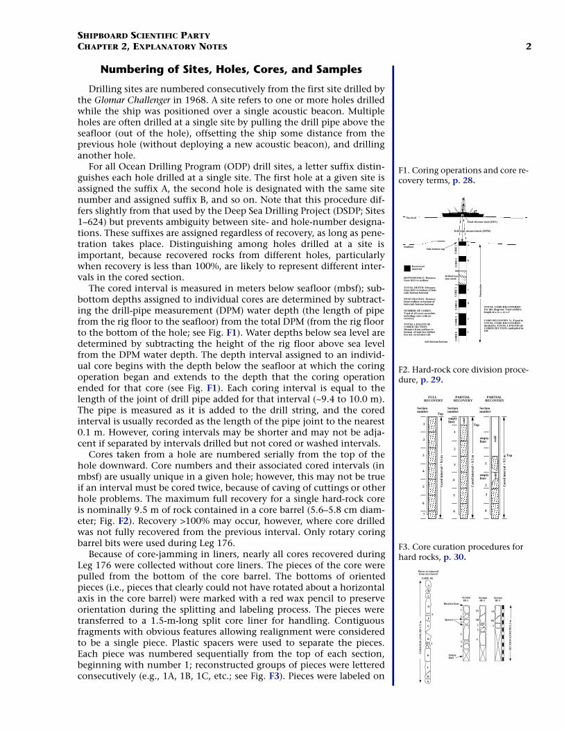
The cored interval is measured in meters below seafloor (mbsf); sub-bottom depths assigned to individual cores are determined by subtract-ing the drill-pipe measurement (DPM) water depth (the length of pipefrom the rig floor to the seafloor) from the total DPM (from the rig floorto the bottom of the hole; see Fig. F1). Water depths below sea level aredetermined by subtracting the height of the rig floor above sea levelfrom the DPM water depth. The depth interval assigned to an individ-ual core begins with the depth below the seafloor at which the coringoperation began and extends to the depth that the coring operationended for that core (see Fig. F1). Each coring interval is equal to thelength of the joint of drill pipe added for that interval (~9.4 to 10.0 m).The pipe is measured as it is added to the drill string, and the coredinterval is usually recorded as the length of the pipe joint to the nearest0.1 m. However, coring intervals may be shorter and may not be adja-cent if separated by intervals drilled but not cored or washed intervals.
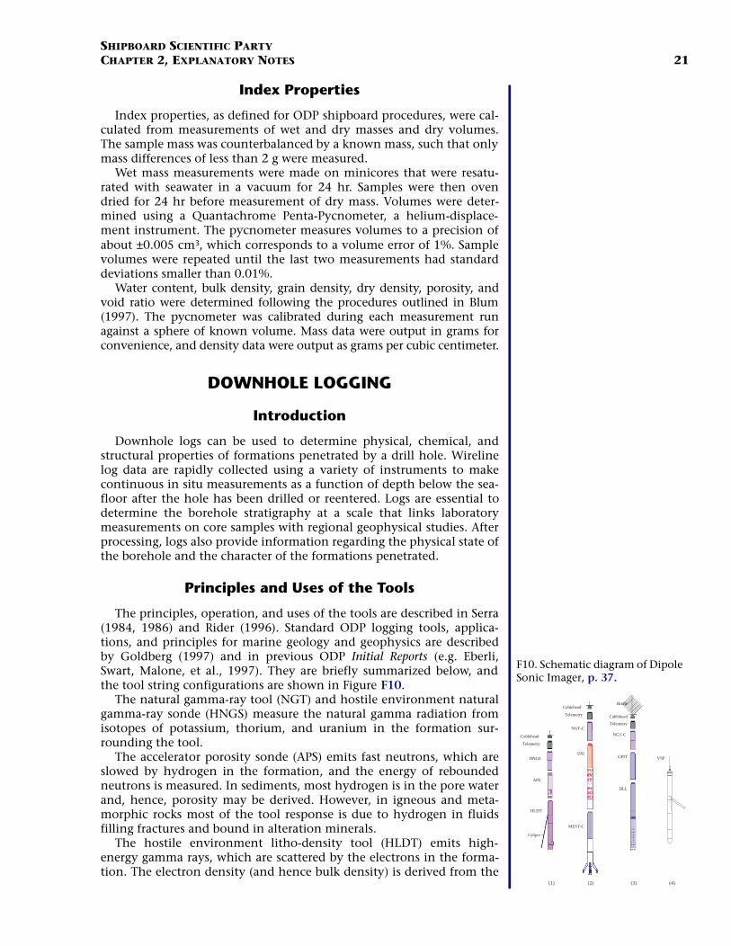
Cores taken from a hole are numbered serially from the top of thehole downward. Core numbers and their associated cored intervals (inmbsf) are usually unique in a given hole; however, this may not be trueif an interval must be cored twice, because of caving of cuttings or otherhole problems. The maximum full recovery for a single hard-rock coreis nominally 9.5 m of rock contained in a core barrel (5.6–5.8 cm diam-eter; Fig. F2). Recovery >100% may occur, however, where core drilledwas not fully recovered from the previous interval. Only rotary coringbarrel bits were used during Leg 176.
Because of core-jamming in liners, nearly all cores recovered duringLeg 176 were collected without core liners. The pieces of the core werepulled from the bottom of the core barrel. The bottoms of orientedpieces (i.e., pieces that clearly could not have rotated about a horizontalaxis in the core barrel) were marked with a red wax pencil to preserveorientation during the splitting and labeling process. The pieces weretransferred to a 1.5-m-long split core liner for handling. Contiguousfragments with obvious features allowing realignment were consideredto be a single piece. Plastic spacers were used to separate the pieces.Each piece was numbered sequentially from the top of each section,beginning with number 1; reconstructed groups of pieces were letteredconsecutively (e.g., 1A, 1B, 1C, etc.; see Fig. F3). Pieces were labeled on
F1. Coring operations and core re-covery terms, p. 28.
Sea level
SeafloorSub-bottom top
CO
RE
1C
OR
E 2
CO
RE
3C
OR
E 6
CO
RE
4C
OR
E 5
a
b
c
d
e
f
Drilled butnot cored
Pen
etra
tion
Recoveredmaterial
Sub-bottom bottom
Dual elevator stool (DES)
BOTTOM FELT- Distancefrom DES to seafloor
TOTAL DEPTH- Distancefrom DES to bottom of hole(sub-bottom bottom)
PENETRATION- Distancefrom seafloor to bottom ofhole (sub-bottom bottom)
NUMBER OF CORES-Total of all cores recorded,including cores with norecovery
TOTAL LENGTH OFCORED SECTION-Distance from seafloor tobottom of hole less drilledbut not cored intervals
TOTAL CORE RECOVERED-For this diagram: Total additivelength of a, b, c, d, e, f
CORE RECOVERY %- Equal toTOTAL CORE RECOVEREDdivided by TOTAL LENGTH OFCORED SECTION, multiplied by100
Drill pipe measurement (DPM)
F2. Hard-rock core division proce-dure, p. 29.
Sectionnumber
1
2
3
4
5
6
7
1
2
3
4
void
Sectionnumber
Sectionnumber
FULLRECOVERY
PARTIALRECOVERY
PARTIALRECOVERY
Cor
ed in
terv
al =
9.5
m
6
5vo
idvo
id
4
3
2
1
emptyliner
emptyliner
emptyliner
Top
Top
Top
Cor
ed in
terv
al =
9.5
m
Cor
ed in
terv
al =
9.5
m
1A
1B
2
3
4
1R-2
Pieces as removed from core barrel
CU
RA
TE
D L
EN
GT
H 2
.75
m
CORE 1R
H
I
1
2
3
4
5
6
1R-1
2
1R-3
A
B
C
D
E
F
G
J
K
L
M
N
Butylate liner
Spacers
Section Section Section
SEC
TIO
N L
EN
GT
H 1
.5 m
Emptyliner
1A
1B
F3. Core curation procedures for hard rocks, p. 30.

SHIPBOARD SCIENTIFIC PARTYCHAPTER 2, EXPLANATORY NOTES 3
external surfaces, and, if oriented, a this-way-up arrow was added to thelabel.
Recovery rates were calculated based on the total length of a corerecovered divided by the length of the cored interval (see Fig. F1). Asmost hard-rock coring operations are characterized by <100% recovery,the spacers between pieces can represent intervals of no recovery up tothe difference in length between a cored interval and the total corerecovered. Of the more than 120 cores recovered during Leg 176, 18had a curated length in excess of the cored interval. While this is notunique when sampling sediments (gas expansion in the core linerscauses anomalously high curated core lengths), it is problematic whendealing with curation of hard-rock cores (which do not expand). In 15of the 18 circumstances, the error is <5% and is almost certainly causedby misestimation of the depth of penetration at the rig floor. Duringmost of the Leg 176 operations, rig floor heave was >2 m; error of 20-30cm in depth of penetration yields 2-3% error in recovery calculations.In all other cases, the incidence of high recovery was immediately pre-ceded by a lower recovery core. Amount of unrecovered core in the pre-vious cored interval was invariably greater than the amount of materialoversampled and was likely caused by a piston of rock that was leftbehind as a core barrel was retrieved, only to be picked up on the subse-quent coring run. Since the database was not designed to process coresstarting at a level above the depth of penetration of the previous core,we could not make this correction to archived data. The interestedreader should be aware of these anomalies, however, and account forthese discrepancies when using curated length or recovery data. Allcores recovered during Leg 176 were designated “R” (rotary drilled) forcuratorial purposes. For detailed descriptions of each core sampled,including photographs of each core, and for thin-section descriptions,see the “Core Descriptions” contents list. Also included on this CD-ROM are logs that list details of Leg 176 photomicrographs (see “Photo-micrographs” contents list).
Summary Core Descriptions
As an aid to the interested investigator, we have compiled summaryinformation of core descriptions on a section-by-section basis and pre-sented these on hard-rock visual core description (HRVCD) forms (seethe “Core Descriptions” contents list). These forms summarize theigneous, metamorphic, and structural character of the core, and presentgraphical representations of the pieces recovered and the lithologicunits identified (see Fig. F4). The far right side of these forms presentsan image of the archive half of the core captured shortly after splitting.To the right side of the image, several columns contain informationabout the core. In left-to-right sequence, these columns includearchived piece numbers and a graphic representation of piece shapewith additional details (veins, fractures, etc.) added to help distinguishfeatures in the image. Next to these is a column indicating pieces thatcould be oriented relative to the core top and a vein number column forcorrelation with a vein log (see “Metamorphic Petrology,” p. 10). Thenext column indicates the location of shipboard samples. For reference,the samples noted conform to the sampling code in the JANUS database(XRF = X-ray fluorescence analysis; TSB = polished thin-section billet;PMAG = paleomagnetic samples, most of which were passed to thephysical properties laboratory; and XRD = X-ray diffraction analysis). Agraphic lithology column illustrates changes in lithologic units (see
CORE/SECTION
176-735B-89R-1
100
150
140
130
120
110
90
80
70
60
50
40
30
20
10
0
H
M
H
M
H
PMAG
1
2
3
4A
4B
5
6
495
496
Interval 495: TROCTOLITIC GABBRODepth in Depth
Interval Location: Core Section Section Piece mbsfUpper contact: 88 1 4 1 500.04Lower contact: 89 1 125 6 502.30Thickness: 2.29 m
Grain Size:Mode Max Min Size Shape/Habit
Plagioclase 60 10 3 coarse tabular /subhedral
Clinopyroxene 35 100 2 coarse equant/oikocrysticanhedral
Olivine 10 25 3 coarse amoeboidal/anhedral
Opaques 0.5Total 105.5**Major phases estimated to ± 5%Modal name (calculated): Olivine GabbroGrain Size: Medium
Type DistributionStructure: intergranular evenly distributedFabric N/A N/AComments: Olivine heavily altered in zones next to fractures. Someclinopyroxene elongated. Clinopyroxene mode variable (5%-40%). Locallygranular. Pegmatitic clinopyroxene from 32-40 cm. Poikilitic clinopyroxenefrom 72-76 cm.
Alteration:Dark green amphibole:
Total Percent: <15Mode of occurrence: Mainly after clinopyroxene, partly after olivine.Comments: As alteration rims, secondary plagioclase.
Secondary plagioclase:Total Percent: <20Mode of occurrence: Replacing primary plagioclase.Comments: Irregularly distributed.
Talc, oxides and (chlorite):Total Percent: <2Mode of occurrence: Replacing olivine.Comments: As mixures in the crystal crack network and aroundcrystals (green amphinbole and dark blue chlorite).
Oxyhydroxides and smectites:Total Percent: <2Mode of occurrence: Replacing olivine relics.Comments: Mixture of orange-red clays and carbonates with earlymetamorphic assemblages.
Carbonates:Total Percent: <1Mode of occurrence: In veins and replacing olivine.Comments: Weathering of olivine is related to carbonate veinformation.
Background Alteration:Degree of alteration: moderate (30%-40%). Olivine is largely replaced byamphibole, talc, and oxides (ca. 80%). Clinopyroxene is rimmed by amphibole(ca. 5%). Plagioclase is partly recrystallized (5%). Superimposed to this high-temperature alteration is weathering of olivine relicts along cracks and carbonateveins.
Vein/Fracture Filling:Amphibole veins in Pieces 1 and 4A are 7 cm in length, 0.5-0.6 mm wide.Carbonate veins in Pieces 3,4A, 5, and 6 are 4-6 cm in length, 0.5-1.0 mm wideand are associated with pervasive oxidation of olivine.
Structures:Mf>V; Mf>JThis section does not contain plastic deformation. Igneous texture can beobserved along the complete section. Magmatic fabric is null or weak (0,1).One narrow cataclastic zone (<1cm) overprints the magmatic texture at the topof the section (Piece 1). A few veins and joints. Arrays of subvertical cracks ormicroveins are often visible in big plagioclases and pyroxenes.
Interval 496: See next section
1
2
3
4
5
Gra
phic
Rep
rese
ntat
ion
Pie
ce n
um
ber
Measu
rem
ent I
D
Str
uctu
re
Lith
olog
ic u
nit
Shi
pboa
rd s
tudi
es
Orie
nta
tion
Str
uct
ure
Met
amor
phis
m
Vei
ns
Gra
phic
Lith
olog
y
cm
F4. Example of hard-rock VCD form, p. 31.

SHIPBOARD SCIENTIFIC PARTYCHAPTER 2, EXPLANATORY NOTES 4
“Igneous Petrology,” p. 4); lithologies recovered are represented by thepatterns illustrated in Figure F5. A unit number corresponds to eachlithologic unit and is recorded in the next column. Metamorphic inten-sity intervals are represented by uppercase letters (see “MetamorphicPetrology,” p. 10). We also present a graphic representation of struc-tural features in the core and a column noting particular structural fea-tures (see “Structural Geology,” p. 13). On the right side of these formsis a text summary of observations from each section. The upper andlower contacts of each lithologic interval are noted, as are primarylithology and other comments summarized from igneous descriptions.Text summaries of metamorphic and structural description for each sec-tion are also compiled on these forms.
IGNEOUS PETROLOGY
General Procedures
Procedures used during Leg 176 for describing igneous rocks in gen-eral follow the outline presented in the “Explanatory Notes” chapter ofLeg 153 (Shipboard Scientific Party, 1995), and much of the discussionpresented here comes from that source. Observations on hard-rockpetrology and petrography were stored in ODP written and electronicmedia and in Excel spreadsheet files according to the definitions givenbelow and the terminology and outlines described in “Linked Spread-sheets,” p. 8. For a detailed discussion of the hard-rock core “barrelsheets,” the reader is referred to “Introduction,” p. 1. Hard-rock macro-scopic observations of igneous rocks were recorded on HRVCD forms bythe igneous petrologists.
Measurements were not made in traditional ODP shift mode butwere performed by the entire igneous petrology group working in tan-dem. For consistency in the measurements, qualitative measurements(especially the selection of igneous contacts) were made by the entiregroup. Each quantitative measurement (e.g., grain size, mode, etc.) wasmeasured by a single team member through the entire core. This, webelieve, resulted in a better and more consistent measurement of mac-roscopic features than is possible by teams working in shifts.
Igneous units were defined on the basis of primary igneous litholo-gies and textures. Mineral modes were estimated (each mineral by anindependent observer), totaled, and rechecked if the total was not100% ± 10%. Plagioclase and augite were estimated to ±5%. Because theabundance of each mineral was determined independently, there is noconstraint that would require a total of 100% for the mode, as would bethe case if a single observer estimated the abundance of all the miner-als. Inasmuch as the total derived by this method provides an indica-tion of the accuracy of the method, the modes were not arbitrarilyrenormalized to 100%. Mineral habits, igneous structures, and igneousfabrics were also recorded, as well as the nature of igneous contacts.Observations were recorded in Excel spreadsheets for each lithologicunit in the core. Details of the individual measurements are givenbelow.
Differences between Leg 176 and Leg 118 VCDs
Differences in the procedures used during Legs 118 and 176, and theopportunity to incorporate insights into the geology of Hole 735B
F5. Graphic lithology patterns used, p. 32.
Gabbro
Oxide gabbro
Olivine gabbro
Oxide olivine gabbro
Gabbronorite
Oxide gabbronorite
Microgabbro
Oxide troctolite
Diorite
Clinopyroxenite
Troctolite

SHIPBOARD SCIENTIFIC PARTYCHAPTER 2, EXPLANATORY NOTES 5
gained on the earlier leg, have resulted in significant differences in thepresentation of the macroscopic visual core descriptions (VCDs) of Leg176. The Leg 118 report recognized only six major lithotectonic units inthe Hole 735B core. A subsequent redescription of the core dividedthese units into 495 primary igneous lithologic intervals (Dick et al.,1991b). The description of the core during Leg 176 extended the philos-ophy of that later study, but the larger group involved in the descrip-tion enabled a more extensive set of measurements to be made.
To provide some continuity between these three studies, the lower 50m of the Leg 118 core from Hole 735B was redescribed using the newsystem. This is illustrated in Figure F6, where the interval sequencesderived by the two data sets are shown side by side. As much as possiblethe old interval numbers were retained in the new description. Whereold intervals were subdivided by the new description, they were labeledA, B, C, and so forth. Where old units were not recognized in the newdescription, the interval numbers of the old description were skipped inthe new sequence.
Rock Classification
The classification of mafic phaneritic rocks recovered during Leg 176closely follows the International Union of Geological Sciences (IUGS)system (Streckeisen, 1974; Le Maitre, 1989; Figs. F7, F8). Minor modifi-cations were made to subdivide the rock types more accurately in theHole 735B core on the basis of significant differences rather than arbi-trary cutoffs based on the abundance of a single mineral. For gabbroicrocks, the modifier “disseminated oxide” is used when the abundanceof Fe-Ti oxide is 1%–2%, and the modifier “oxide” is used when theabundance is >2%. The terms “orthopyroxene-bearing gabbro” and“gabbronorite” are used to denote the presence of discrete orthopyrox-ene grains; orthopyroxene present as reaction rims is ignored for thepurpose of assigning a rock name. Rocks with between 1% and 5%orthopyroxene are called orthopyroxene-bearing gabbros and sampleswith >5% orthopyroxene are called gabbronorite. The term “troctolitic”is used to describe olivine gabbros with 5%–15% clinopyroxene and therock name “troctolite” is used for rocks with <5% clinopyroxene.“Anorthositic” is used for gabbros with >80% plagioclase. High propor-tions (>65%) of mafic minerals are noted by the prefix mela-, and highproportions (>65%) of plagioclase are noted by the prefix leuco-. Themodifier “micro” is used to distinguish gabbroic rocks with a dominantgrain size of <1 mm (e.g., microgabbro, microtroctolite, and microgab-bronorite). Leucocratic rocks with >20% quartz and <1% K-feldspar (arestricted part of the “tonalite” field of the IUGS system) are called“trondhjemites” in keeping with previous usage in the ocean crust liter-ature. On the HRVCDs, the rock names as described above are given atthe top of each interval description, the official IUGS names calculatedfrom the mode are given in the text.
If a mafic rock exhibits the effects of dynamic metamorphism suchthat the assemblage consists of secondary hydrous minerals that com-pletely obliterate the protolith mineralogy and texture, or if the rock ismade up of recrystallized primary minerals such that the original igne-ous protolith cannot be recognized, the appropriate metamorphic rocknames are used. The textural terms “mylonitic,” “schistose,” and“gneissic” are added to metamorphic rock names, such as “greenstone,”“amphibolite,” or “metagabbro” to indicate that the rocks exhibit theeffects of dynamic metamorphism. The methods for describing the
F6. Legs 176, 118 lithostratigraph-ic intervals compared, p. 33.
438a
439439
440 440
450
452
454
456
458
460
462
464
466
468
470
472
474
442 442
444 444
446
447
448 448
451
449451451a
452452
452a
452c
453
453
457
457456d
455456a
476
478
480
482
484
486
488
490
492
494
496
498
500
461
460
460b
462462
465a
466
469a
469b
471
473a
474
474
471
470
469
466
467
475 475
476 476
477
478
482
476a
476b
477
480
482
492
485
486
487
484a484b
487
491a
493
Depth(mbsf)
Leg 176intervals
Leg 118intervals
Depth(mbsf)
Leg 176intervals
Leg 118intervals
447
463 463
446
F7. Classification of ultramafic and gabbroic rocks, p. 34.
olivineplagioclase plagioclase
plagioclase
orthopyroxeneclin
opyr
oxen
e
dunitetroctolite troctolite
gabb
ro
wehrlite
harz
burg
ite
norite
websterite
gabbronorite
gabb
ro norite
olivinewebsterite
olivine gabbro olivine noritelherzolite
clinopyroxenite
orthopyroxenite
anorthositeanorthosite
anorthosite
oliv
ine
orth
opyr
oxen
ite
olivine
clinopyroxenite
90
5
40
F8. Classification of silicic pluton-ic rocks, p. 35.
granite
granodiorite
tonalite
quartz diorite
dioritemonzodioritemonzonite
quartzmonzodiorite
quartzmonzonite
syenite
quartz syenite
alkali feldspar quartz syenite
alkali feldspar syenite
alkalifeldspar plagioclase10 35 65 90
5
20
60
alka
li fe
ldsp
ar g
rani
te
quartz
granitoids

SHIPBOARD SCIENTIFIC PARTYCHAPTER 2, EXPLANATORY NOTES 6
metamorphic and structural petrology of the core are outlined in subse-quent sections of this chapter.
Primary Silicate Minerals
The principal rock-forming silicate minerals in the core are plagio-clase, olivine, clinopyroxene, and orthopyroxene. For each of theseminerals, the following data were recorded in the HRVCDs and in Excelspreadsheets: (1) estimated modal percent of the primary minerals; (2)smallest and largest size of mineral grains (measured along the longestaxis in millimeters); (3) average crystal size for each mineral phase usingfine-grained (<1 mm), medium-grained (1–5 mm), coarse-grained (5–30mm), and pegmatitic (>30 mm); (4) mineral shapes using terms such asequidimensional, tabular, prismatic, platy, elongate, acicular, andamoeboidal; (5) mineral habit using the terms euhedral, subhedral,anhedral, rounded, deformed, and fractured; and (6) mineral occur-rence if minerals occurred as chadacrysts or oikocrysts.
Primary Fe-Ti Oxide and Sulfide Mineralogy
The abundance of oxides in the core was visually estimated using abinocular microscope with 10× magnification. A continuous log ofoxide abundance was compiled along with average abundances in eachinterval. Oxide habits in hand sample are divided into the followingcategories: disseminated, interstitial network, concordant seams, discor-dant seams, and matrix. There is a strong correlation between the tex-tures and abundance. “Disseminated” is used to describe scatteredgrains or grain clusters of oxides with no pronounced fabric, and ismost commonly observed in samples with low oxide abundances.“Interstitial network texture” is used to describe oxides that occur inter-stitial to the silicates, surrounding or partially surrounding groups ofsilicate grains, and was most commonly observed in samples with lowto moderate oxide abundances. “Concordant seams” is used to describethin, elongate lenses or patches of oxides parallel to the silicate fabric,and “discordant seams” is used to describe those that crosscut the sili-cate fabric. Both types of seams are most commonly observed in sam-ples with low to moderate oxide abundances. “Matrix” is used todescribe continuous networks of oxides that completely surround andseparate the silicate phases and is most commonly observed in sampleswith high oxide abundances. Oxide shapes in hand sample are dividedinto the following categories: euhedral, anhedral, angular aggregates,amoeboidal aggregates, and interstitial lenses. “Euhedral” and “anhe-dral” are used when it appeared that isolated individual grains werepresent; “aggregates” are used to describe what appeared to be contigu-ous grain clusters.
Relative sulfide abundance in hand specimen was estimated using a10× binocular microscope and a scale of 0 to 5, where 0 = not observed,1 = rare, 2 = average, 3 = above average, 4 = abundant, and 5 = veryabundant. Many samples contain sulfide grains too small to be seen onthe saw-cut surface at 10× magnification, and for these samples the esti-mated abundances are too low. Sulfide habits in hand specimen aredivided into the following categories: disseminated, disseminated withoxides, disseminated in silicates, concordant seams, discordant seams,clusters with oxides, clusters in silicates, and massive. “Disseminated insilicates” is used to describe low concentrations of scattered sulfidegrains enclosed in silicates, and “disseminated with oxides” is used to

SHIPBOARD SCIENTIFIC PARTYCHAPTER 2, EXPLANATORY NOTES 7
describe low concentrations of scattered sulfide grains enclosed ineither silicates or oxides but associated with oxide concentrations.“Concordant seams” is used to describe thin, elongate lenses or patchesof sulfides parallel to the silicate fabric, and “discordant seams” is usedto describe thin, elongate lenses or patches of sulfides that crosscut thesilicate fabric. “Clusters in silicates” is used to describe sulfide grainsthat are present near other sulfide grains, and are included in silicates,and “clusters with oxides” is used to describe sulfide grains that arepresent near other sulfide grains included in either silicates or oxidesbut associated with oxide concentrations. Massive is used to describelarge patches or lenses of sulfides with an average dimension >1 cm.Sulfide shapes in hand sample were divided into the following catego-ries: euhedral, anhedral, globular inclusions, angular inclusions, globu-lar interstitial, and angular interstitial. “Euhedral” and “anhedral” areused when isolated individual grains are present; “globular” and “angu-lar” are used to describe what appear to be contiguous grain clustersthat are nearly spherical masses or are not nearly spherical, respectively.
Igneous Textures
Textures of igneous rocks are characterized on the basis of grain size,grain shape, preferred mineral orientation, and mineral proportions.The dominant grain size for each unit is recorded as fine grained (<1mm), medium grained (1–5 mm), coarse grained (5–30 mm), or pegma-titic (>30 mm). Rock textures such as “equigranular,” “inequigranular,”“intergranular,” and “granular” are used to describe the overall textureof each lithologic unit. “Poikilitic,” “ophitic,” and “subophitic” texturesare distinguished according to the predominant grain shapes in eachunit. Igneous fabrics that are distinguished include “lamination” forrocks exhibiting a preferred orientation of mineral grains that was likelyderived from magmatic processes, “clusters” for mineral aggregates, and“schlieren” for lenses of igneous minerals.
Igneous Structures
Igneous structures noted in the core description include layering,gradational grain-size variations, gradational modal variations, grada-tional textural variations, and breccias. “Layering” is used to describeplanar changes in grain-size, mode, or texture within a unit. Grain-sizevariations are described as normal if the coarser part was at the bottomand as reversed if the coarser part was at the top. Modal variations aredescribed as normal if mafic minerals are more abundant at the bottomand as reversed if mafic minerals are more abundant at the top. “Igne-ous breccia” is noted where the breccia matrix appears to be of mag-matic origin.
Contacts between Lithologic Intervals
The most common types of contacts are those without chilled mar-gins. These are either planar, curved, irregular, interpenetrative,sutured, or gradational. Sutured refers to contacts where individualmineral grains are interlocking across the contact. In many cases, con-tacts are obscured by subsolidus or subrigidus deformation and meta-morphism and are called “sheared” if an interval with deformationfabric is in contact with an undeformed interval, “foliated” if both

SHIPBOARD SCIENTIFIC PARTYCHAPTER 2, EXPLANATORY NOTES 8
intervals have deformation fabrics, or “tectonic” if the contact appearsto be the result of faulting.
Thin-Section Description
Thin sections of igneous rocks were examined to complement andrefine the hand-specimen observations. In general, the same type ofdata were collected from thin sections as from hand-specimen descrip-tions, and a similar terminology is used. Modal data were collectedusing standard point-counting techniques. All data are recorded in thethin-section spreadsheet (see “Appendix,” p. 31, in the “Leg 176 Sum-mary” chapter) and summarized in ODP-format thin-section descrip-tions (see the “Core Descriptions” contents list). Crystal sizes weremeasured using a micrometer scale and are generally more precise thanhand-specimen estimates. The presence of inclusions, overgrowths, andzonation is noted, and the apparent order of crystallization is suggestedin the comment section for samples with appropriate textural relation-ships. The presence and relative abundance of accessory minerals suchas oxides, sulfides, apatite, and zircon are noted. The percentage ofalteration is also reported (see “Metamorphic Petrology,” p. 10).
Linked Spreadsheets
Because the hard-rock application of JANUS was not yet complete,and the old database (HARVI) had been discontinued, igneous data col-lected during this leg are recorded in a set of linked Microsoft Excelspreadsheets. There are five interlinked spreadsheets (I_LITH.XLS,I_TEX.XLS, I_MIN.XLS, I_COMM.XLS, and DEPTHS.XLS) and threeindependent spreadsheets (I_OPAQUE.XLS, I_VEIN.XLS, and176GEOCH.XLS) in this collection (For detailed information on thespreadsheets, see “Appendix,” p. 31, in the “Leg 176 Summary” chap-ter). The interlinked spreadsheets cover lithologies, mineralogy, tex-tures, and comments. Most data in these spreadsheets are recorded asnumerical values, and the numeric codes are translated to English andback via a pair of “Visual Basic for Applications” (VBA) look-up macros.Information about igneous contacts is recorded in the lithology spread-sheet (I_LITH.XLS). This includes information about the position ofthe contact, its depth, the thickness and type of rock above the contact,the type of contact (e.g., igneous or tectonic), and the form of the con-tact (e.g., planar or curved).
The other three databases link to the I_LITH.XLS spreadsheet col-umns defining the position of the lower contact of each interval. TheI_MIN.XLS spreadsheet additionally records the mode of the igneousminerals (plagioclase, clinopyroxene, olivine, orthopyroxene, oxides,and sulfides), as well as the grain size of the silicate minerals (plagio-clase, clinopyroxene, olivine, and orthopyroxene). From these data, arock name is automatically generated by a VBA macro. The I_TEX.XLSspreadsheet records mineral shapes (e.g., acicular, platy, etc.) and habits(e.g., chadacrystic, ophitic, etc.). The I_COMM.XLS spreadsheet con-tains number codes for igneous textures and fabrics, as well as text com-ments on each interval. An independent (unlinked) spreadsheet,I_OPAQUE.XLS, records the approximate oxide abundance in therecovered core on a centimeter by centimeter basis.
An independent (unlinked) spreadsheet, I_VEIN.XLS, records thedata on “trondhjemite veins.” Here, “trondhjemite” represents any ofthe various quartzo-feldspathic igneous rocks that were recovered
Note: To open the Excel spread-sheets, either click on the file-names in the text or open the files through Microsoft Excel. To use the in-text links, your computer must be configured to automati-cally launch Microsoft Excel when files with .XLS extensions are opened. The spreadsheet files can be found in the \176_IR\SUPP_MAT\APPENDIX\ directory on the CD-ROM.

SHIPBOARD SCIENTIFIC PARTYCHAPTER 2, EXPLANATORY NOTES 9
(including tonalite and granodiorite), it being the most common.Trondhjemite of apparent igneous origin that crosscuts the core, andthat is more than 5 cm in thickness along the length of the core, isrecorded as a separate lithologic interval. Trondhjemite of igneous orhydrothermal origin that is less than 5 cm in thickness along the lengthof the core is recorded as a vein. Although this is an arbitrary cutoff, itprovides a workable solution for the description of the hundreds of thintrondhjemite dikelets, fracture fillings, and/or veins that cut the core.The I_VEIN.XLS spreadsheet records the position and igneous intervalof each trondhjemite vein, the apparent thickness relative to the verti-cal axis of the core, the true thickness perpendicular to the plane of thevein, the thickness of the zone in which the vein or vein networkoccurs, the percentage by area of trondhjemite within that zone, andcomments about the vein. Although many of the thicker “veins”appear to be of igneous origin, for many of the veins it is not possible inhand specimen to determine whether they are of igneous or hydrother-mal origin. Although the log excludes veins of clearly hydrothermal ori-gin, it includes any veins of unclear origin.
A macro in the I_MIN.XLS file extracts a condensed data report oneach igneous interval. This macro is accessed from the “Report” work-sheet of the I_MIN.XLS spreadsheet. All other spreadsheets must firstbe loaded and translated using their respective “Translate” buttons;then the Up and Down buttons on the report page scroll through theentire database one line at a time. It is possible to jump to any part ofthe database by typing an interval number in the appropriate cell andpressing the “Go” button. This loads the values from that interval intothe report and copies the entire report onto the (Windows or Mac) clip-board.
Multi-interval reports are generated by switching to the “Mineral-ogy” worksheet and highlighting a group of interval numbers, switch-ing back to the report sheet and pressing the “Multi” button. Thecorresponding unit reports are formatted and transferred via OLE toMicrosoft Word. Word is then brought to the foreground, where furtherediting can take place.
Depths below seafloor for the igneous spreadsheets and for otherpurposes are calculated using the EDepth and CDepth functions of theDEPTHS.XLS spreadsheet. This spreadsheet by default hides itself afterloading. Its functions can be used by selecting the Tools|Add-ins menuitem in Excel. From the Add-in manager dialog box select “Browse,”and go to the DPTHSMTH\EXCOM directory where DEPTHS.XLSresides. Double click on DEPTHS.XLA to install this add-in to Excel. If adialogue box asks you to copy the add-in to the Microsoft DefaultLibrary, it is important to select “NO.” The item “Hole 735B Depths”should now be listed as an item in the Add-in manager. It is now perma-nently installed in Excel until the checkbox next to its name is dese-lected, which will uninstall it. The depth calculator will now reloadautomatically every time Excel is started. To use the depth calculator,type in a destination cell
=EDepth(A1,B1,C1/100).
Make sure to replace A1 in this equation with the cell where the corenumber of interest resides, making sure that the core number is an inte-ger rather than the alphanumeric combination (i.e., 90 instead of 90R).Replace B1 with the cell where the section number of interest residesand C1 with the cell where curated depth in the section resides (in cm).
Note: Add-in functions may not operate in all versions of Microsoft Excel.

SHIPBOARD SCIENTIFIC PARTYCHAPTER 2, EXPLANATORY NOTES 10
Expanded/compressed depth should appear in the destination cell,which can be copied and pasted to subsequent cells.
An additional add-in menu item was also written that calculates aspatial moving average of irregularly spaced data points. This add-initem resides in the DPTHSMTH directory in a subdirectory namedSMOOTH. The “Smooth” add-in is installed the same way as the depthscalculation add-in (see above). Once the add-in is installed, it adds theitem “Smooth” to the Tools menu. To use this function, make sure thereis a free column in a destination spreadsheet for the output. Depths andvalues for those depths must reside in two other columns. Highlight afew cells of the output destination column and select “Smooth” fromthe tools menu. A “Set-up” dialog box will appear; ensure the destina-tion range is correct. Enter into the cells below the destination rangethe number of columns that the depth and value range are offset fromthe output column and select a smoothing interval. Selecting the “Fast”checkbox speeds up the smoothing process by hiding the individualcell updates. The “Keep Going” checkbox instructs the algorithm tokeep working its way downward as long as there is data to process.Once everything is entered, selecting the “Go” icon should outputsmoothed data to the destination column.
Igneous Lithology, Interval Definitions, and Summary
For a complex sequence of plutonic rocks, interpretations of thevertical lithologic successions in the core are difficult because of over-printing of synmagmatic, metamorphic, and tectonic processes. Thelithologic intervals adopted here are defined by vertical sections withconsistent internal characteristics and lithology and are separated basedon geological contacts defined by significant changes in modal mineral-ogy or primary texture, as encountered downhole. To the extent possi-ble, boundaries were not defined where changes in rock appearancewere only the result of changes in the type or degree of metamorphism,or the intensity of deformation. Both sharp and gradational contactsoccur between intervals. If the contact was recovered, its location isrecorded by the core, section, position (cm), and piece number. If thecontact was not recovered, but a significant change in lithology or tex-ture is observed, the contact is placed at the bottom of the lowest pieceof the upper interval. The information recorded for each section of thecore includes the rock type; igneous, metamorphic, and/or deforma-tional texture; evidence for igneous layering; extent, type, and intensityof deformation; primary, and secondary minerals present; grain shapefor each primary mineral phase; evidence of preferred orientation; theposition of quartzo-feldspathic veins (whether of igneous or hydrother-mal origin); and general comments. The description and summary ofeach interval were entered into the standard ODP-format programwhere the general lithologic description and top and bottom of theinterval are recorded with reference to curated core, section, piece(s),depth, and thickness.
METAMORPHIC PETROLOGY
Visual core descriptions of metamorphic characteristics were com-piled together with igneous and structural documentation of the coreto provide information on the extent of alteration, alteration mineralphases, and vein characteristics. These data were recorded in the Alter-

SHIPBOARD SCIENTIFIC PARTYCHAPTER 2, EXPLANATORY NOTES 11
ation and Vein Logs (for detailed information see “Appendix,” p. 31, inthe “Leg 176 Summary” chapter [BGALTLOG.XLS, VEINLOG.XLS]),respectively, and are summarized in the HRVCDs. To ensure accuratecore descriptions, the petrography of representative samples wasrecorded in the Alteration Thin-Section Log (see “Appendix,” p. 31, inthe “Leg 176 Summary” chapter) and integrated with the visual coredescriptions. Identification of mineral phases was checked by XRDanalyses according to ODP standard procedures outlined in previousInitial Reports volumes (e.g., Volume 118; Shipboard Scientific Party,1989). For each section the following information was recorded: leg,site, hole, core number, core type, section number, piece number (con-secutively downhole), and position in the section.
Macroscopic Descriptions
The metamorphic mineral assemblages and alteration intensity wererecorded in the Alteration Log. Primary phases (olivine, clinopyroxene,orthopyroxene, and plagioclase) and the secondary minerals thatreplace them were noted and, where possible, the volume percent ofeach phase was estimated in hand specimen and checked by observa-tion of representative thin sections. Vein mineralogy, vein length andwidth (measured on the cut face of a piece or pieces), the top and thebottom location of the vein in the piece(s), vein type, vein mineralogyand mineral abundance, associated halo widths, and wall rock alter-ation were recorded in the Vein Log. The length and width of each veinwere used to calculate the vein area; where veins are very abundant (netveins), the percent area of the veins within a piece or interval was esti-mated visually. These data were used to calculate the density of veins inthe core and the volume percentage of each vein type within a giveninterval and within the entire core.
Thin-Section Descriptions
Detailed petrographic descriptions were made aboard ship to aid inidentification and characterization of metamorphic and vein mineralassemblages. Stable mineral parageneses were noted, as were texturalfeatures of minerals indicating overprinting events (e.g., coronas, over-growths, and pseudomorphs). Mineral abundances were either esti-mated visually or determined by point counting. These data arerecorded in the Alteration Thin Section Log and summarized in thethin-section descriptions (see the “Core Descriptions” contents list).The modal data allowed accurate characterization of the intensity ofmetamorphism and aided in establishing the accuracy of the macro-scopic and microscopic visual estimates of the extent of alteration.
GEOCHEMISTRY
Samples considered by the shipboard scientific party to be represen-tative of the various lithologies cored were analyzed for major oxideand selected trace element compositions with the shipboard ARL 8420wavelength-dispersive XRF apparatus. Full details of the shipboard ana-lytical facilities and methods are presented in previous ODP InitialReports volumes (e.g., Legs 118, 140, 147, 153; Shipboard ScientificParty, 1989, 1992, 1993, 1995a). The elements analyzed and the operat-ing conditions for Leg 176 XRF analyses are presented in Table T1. T1. X-ray fluorescence data, p. 39.

SHIPBOARD SCIENTIFIC PARTYCHAPTER 2, EXPLANATORY NOTES 12
After coarse crushing, samples were ground in a tungsten carbideshatterbox. Then 600-mg aliquots of ignited rock powder were inti-mately mixed with a fusion flux consisting of 80 wt% lithiumtetrabo-rate and 20 wt% “heavy absorber” La2O3. The glass disks for the analysisof the major oxides were prepared by melting the mixture in a plati-num mold in an electric induction furnace. Trace elements were deter-mined on pressed powder pellets prepared from 5 g of rock powder(dried at 110°C) mixed with a small amount of a polyvinylalcoholbinder solution. The calibration of the XRF system was based on themeasurement of a set of reference rock powders. A Compton scatteringtechnique was used for matrix absorption correction for trace elementanalysis.
The total sum of the oxides determined on ignited powders was gen-erally high. About 60% of the samples had “totals” between 101% and103%. The systematic analytical error presumably reflects small inade-quacies in the procedure for correction for matrix absorption or errorsin the concentration of the “heavy absorber” in the fusion flux. A smallset of samples was reanalyzed after the cruise by atomic emission andatomic absorption spectrometry at Leuven University, Belgium. Itappeared that the error affects all the major element oxides, but it sig-nificantly affects only the result of the main component SiO2, and tolesser extent of Al2O3, CaO, MgO, and Fe2O3.
A second analytical problem concerned the trace element zirconium.Zirconium data for olivine gabbros obtained during Leg 176 were sys-tematically higher than in equivalent rocks analyzed during Leg 118. Todetermine whether this was a real geochemical difference, a selection ofLeg 118 shipboard powder samples was reanalyzed during Leg 176.Consistently higher Zr values were obtained. A postcruise analysis ofcontrol samples at the Universities of Copenhagen, Denmark, and Leu-ven, Belgium, showed that the lower values obtained during Leg 118are the more accurate ones. Inadequacies in the correction for the inter-ference of Sr X-rays on Zr X-ray peaks are the most likely source of ana-lytical errors. Unfortunately, the problem could not be remedied duringthe cruise. As a consequence, the reported Zr data may be too high by afactor of two in the 15- to 30-ppm concentration range. At higher Zrconcentration levels, the effect of the analytical error is minor.
Loss on ignition (LOI) for each sample was determined by the stan-dard practice of heating an oven-dried (110°C) sample to 1010°C forseveral hours. To more fully investigate the results of LOI determina-tions of selected samples, gas chromatography of the expelled volatileswas performed on a Carlo Erba NA 1500 CHS analyzer; 20 mg of dried(110°C) rock sample was combusted at 1010°C, releasing water and car-bon dioxide. Sulfur from sulfide minerals is oxidized to SO2 (by additionof V2O5), and SO3 is released from any sulfate minerals present in thesample. Gas-chromatographic separation was followed by quantitativedetermination of the respective gaseous oxides of carbon, hydrogen,and sulfur by a thermal conductivity detector. Reagent grade sulfanil-amide (C6H8N2O2S) was used to calculate the bias factor of the analyzerfor CO2, H2O, and SO3. Control rock samples covering the concentra-tion ranges of hydrogen, carbon, and sulfur observed in the cored sam-ples were repeatedly analyzed. These control samples were prepared byintimately mixing weighed quantities of a low-sulfur, low-carbon sili-cate rock (Gaby 153 Interlaboratory Standard prepared during Leg 153)and of sediment sample ODP6 (containing 3.2 wt% C, 0.56 wt% H, and5300 ppm S). Because the concentration of total sulfur in most of the

SHIPBOARD SCIENTIFIC PARTYCHAPTER 2, EXPLANATORY NOTES 13
rock samples was close to the determination limit of the CHS analyzer,results of duplicate analyses for sulfur showed large scatter. Therefore,no results of sulfur analysis are listed in this volume.
After the cruise all the shipboard samples were analyzed for ferrousiron content at the University of Leuven, Belgium, using the redox-titration method of Shafer (1966). Sample aliquots weighing from 50 to100 mg were dissolved in a H2SO4/HF mixture in a nitrogen atmo-sphere. Ferrous iron is titrated with potassium-dichromate solutionusing sodiumdiphenylaminesulfonate as a redox color indicator.
STRUCTURAL GEOLOGY
Conventions for structural studies established during previous “hard-rock” drilling legs (e.g., Legs 118, 131, 140, 147, and 153) were gener-ally followed during Leg 176. However, several minor changes innomenclature and procedure were adopted. These changes aredescribed below. Where procedures followed directly from previouslegs, references to the appropriate Initial Reports “Explanatory Notes”chapter are given.
Overview of Macroscopic Core Description
Because of the high recovery rate during Leg 176, archive halves ofthe cores were stored immediately, and all structural measurements hadto be made on the working halves. Following procedures described inthe Leg 153 Initial Reports volume (Shipboard Scientific Party, 1995a),data were entered into a VCD form (Fig. F4), used in conjunction withfive spreadsheet logs (see “Appendix,” p. 31, in the “Leg 176 Sum-mary” chapter). The structural sketches drawn on the VCD form areintended to illustrate the most representative structures and crosscut-ting relationships present on a core section; in addition, a brief generaldescription of the structures is printed on the same form. Where nomagmatic fabric, or only a weak one, was present (predating any otherstructure), the structural column was left blank.
Paper copies of spreadsheet forms were used for recording specificstructures and measurements during core description. Separate spread-sheets were used to record data on (1) joints, veins, cleavage, and folds;(2) breccias, faults, and cataclastic fabrics; (3) crystal-plastic fabrics andsense of shear indicators; (4) magmatic fabrics, compositional layering,and igneous contacts; and (5) crosscutting relationships. The descrip-tion and orientation of all features were recorded using curated depthso that “structural intervals” could be correlated with other lithologicintervals. The spreadsheets were organized to identify five separatetypes of structural intervals using deformation intensity scales summa-rized in Table T2. The structural geologists worked together during thesame shift to minimize measurement inconsistencies. Each member ofthe team was responsible for making a specific set of observationsthroughout the entire core (e.g., characterization of magmatic fabricintensity). Descriptions and structural measurements were based onobservations on the working half of the core (see orientation of struc-tures below).
T2. Deformation intensity scales, p. 40.

SHIPBOARD SCIENTIFIC PARTYCHAPTER 2, EXPLANATORY NOTES 14
Nomenclature
To maintain consistency of core descriptions, we used feature “iden-tifiers” for structures similar to those outlined in Shipboard ScientificParty (1995a). Modifications to this scheme are shown in the commentschecklist (Table T3) and include designation of breccia type (hydro-thermal - Bh, cataclastic - Bc, or magmatic - Bm). In core sections wherecrystal-plastic fabrics clearly overprint brittle hydrothermal or mag-matic breccia, a note was made in the comment section of the crystal-plastic fabric spreadsheet that deformation occurred in the retrogrademetamorphic assemblage. Where brittle fabrics overprint crystal-plasticfabrics, or deformation was “semi-brittle,” a note was made in the com-ments section and documented in the crosscutting relations spread-sheet.
Structural Measurements
Structural features were recorded relative to core section depths incentimeters from the top of the core section. Depth was defined as thepoint where the structure intersects the center of the cut face of theworking half of the core, as detailed during Leg 153 (see fig. 15A inShipboard Scientific Party, 1995a). Crosscutting relationships weredescribed in intervals delimited by top and bottom depth.
Apparent fault displacements were recorded as they appeared on thecut face of the archive half of the core and the end of broken pieces.Displacements seen on the core face were treated as components of dip-slip movement, either normal or reverse. Strike-slip displacements ofvertical features were termed either sinistral or dextral. Displacementsof features visible on the upper and lower surfaces of core pieces weretreated as components of strike slip and termed sinistral or dextral. Dis-placements were measured between displaced planar markers, parallelto the trace of the fault. Additional cuts and slickenside orientationswere incorporated wherever possible to differentiate among apparentdip slip, oblique slip, and strike slip.
The structures were oriented with respect to the core reference frame;the convention we used for the core reference frame is explained inShipboard Scientific Party (1995a) and shown at the top of the com-ments box in the structural data spreadsheets (see “Appendix,” p. 31,in the “Leg 176 Summary” chapter).
Planar structures were oriented using the techniques outlined duringLegs 131 and 153 (Shipboard Scientific Party, 1991; 1995a). Apparent-dip angles of planar features were measured on the cut face of the work-ing half of the core. To obtain a true-dip value, a second apparent-dipreading was obtained where possible in a section perpendicular to thecore face (second apparent orientation). Apparent dips in the cut planeof the working core were recorded as two-digit numbers (between 00°and 90°) with a dip direction to 090° or 270°. In the “second” plane,apparent-dip directions were recorded as either 000° or 180°. The dipand the dip direction with respect to the working half of the core wererecorded on the spreadsheet together with second plane measurements.If the feature intersected the upper or lower surface of the core piece,measurements were made directly of the strike and dip in the core refer-ence frame. Where broken surfaces exposed lineations or striations, thetrend and plunge were measured directly, relative to the core referenceframe.
T3. Checklist used for spreadsheet comments, p. 41.

SHIPBOARD SCIENTIFIC PARTYCHAPTER 2, EXPLANATORY NOTES 15
The two apparent dips and dip directions measured for each planarfeature were used to calculate a true dip. These calculations were per-formed using either (1) LinesToPlane by S.D. Hurst or (2) App2truedipby B. Celerier (see “Appendix,” p. 31, in the “Leg 176 Summary” chap-ter). Calculated data can be read directly into the shareware stereonetplotting program Stereoplot 3.05 of Neil Mancktelow.
Deformation Intensities
A semiquantitative scale of deformation intensities was used by theshipboard structural geologists during core description. This scale,shown in Table T2, has been modified from the deformation scale usedduring Leg 147 (table 2 in Shipboard Scientific Party, 1993) and the fab-ric intensity scales used during Leg 153 (fig. 13 in Shipboard ScientificParty, 1995a) and conforms to the scales for deformation textures usedby Cannat et al. (1991) and Dick et al. (1991b) in the Leg 118 ScientificResults volume. Wherever possible we have assigned specific values tointensity estimates (e.g., the spacing of veins; the percentage of matrixin a cataclastic zone) to maintain consistency throughout the core.However, for some categories this proved difficult (e.g., the intensity ofany crystal-plastic fabric) in which cases we have used qualitative esti-mates of intensity based on hand-specimen and thin-section observa-tions. We chose five distinct types of deformation for intensitymeasurements (Table T2):
1. Magmatic: The presence and intensity of any shape-preferredorientation of magmatic phases. Four levels, from no shape-preferred orientation (0) to a strong shape-preferred orientation(3), were used.
2. Crystal-plastic: Six levels of deformation intensity were used,ranging from a lack of any crystal-plastic fabric, through twostages of foliation development, and finally to (ultra)myloniticfabrics.
3. Cataclastic: Six levels of deformation intensity were used withfabrics categorized depending on the percentage of matrixpresent within each cataclastic zone. Thin-section descriptions,wherever possible, significantly aid this categorization.
4. Joints (fractures): Four levels of joint density were used, depend-ing on the average frequency of joints across a 10-cm depth in-terval along the long axis of the core. Joints were distinguishedfrom faults (cataclastic features) by the lack of any identifiableoffset.
5. Veins: The same four-level scale of density used for joints was in-corporated for veins. However, where there was an identifiableoffset across a vein, it was treated as a fault rather than a vein.The widths of individual veins were measured by the metamor-phic team and entered into the vein log.
Occasionally it proved difficult to differentiate between crystal-plasticand cataclastic deformation in relatively high-strain shear zones basedon hand-specimen observations only. For this reason, as during Leg 147,we have tried to classify both of these deformation styles using parallelscales where a certain intensity of cataclasite is a direct equivalent to thesame intensity of crystal-plastic deformation.
Initial inspections of the core indicated a prevalence of small, sub-horizontal microfractures throughout the core; to avoid unnecessary
Note: Stereoplot only works on Macintosh computers running OS version 8.1 or lower.

SHIPBOARD SCIENTIFIC PARTYCHAPTER 2, EXPLANATORY NOTES 16
measurements of these regular features, a column was introduced intothe structural spreadsheet to indicate the density of these features usingthe same density scale as for joints. The microfractures, which werelikely induced by drilling, have been termed “subhorizontal microfrac-tures” (SHM).
Thin-Section Descriptions
Thin sections were examined to characterize the microstructuralaspects of important mesoscopic structures in the core. Classes of infor-mation that were obtained include deformation mechanisms on a min-eral-by-mineral basis, kinematic indicators, crystallographic and shapefabrics, qualitative estimates of the degree of crystallographic preferredorientation along local, principal finite strain axes, syn- and post-kinematic alteration, and the relative timing of microstructures.
The orientation of thin sections relative to the deformation fabricsand core axes is noted in the comments section of the spreadsheet.Thin sections were oriented, where possible, with respect to the coreaxis and in the core reference frame described in “Structural Measure-ments,” p. 14. Selected samples were cut perpendicular to the foliationand parallel to any lineation to examine kinematic indicators and theshape-preferred orientation of minerals (see fig. 15, Shipboard ScientificParty, 1995a). We adopted and modified the thin-section descriptionform used by the structural geologists during Leg 140 (Shipboard Scien-tific Party, 1992) to enter the microstructural information into thespreadsheet database.
The terms used to describe microstructures generally follow thoseused during Leg 153. Microstructures of gabbroic rocks recovered at Site735 are discussed in detail in “Igneous Petrology,” p. 12, and “Struc-tural Geology,” p. 54, in the “Site 735” chapter. Although a large spec-trum of microstructures occurs, for the purposes of entering data intospreadsheets a number of textural types characterized by specific micro-structural styles were defined and are keyed to the spreadsheet. Theseare summarized for gabbroic rock in Table T4.
It is possible that superposition of different microstructures or defor-mation mechanisms may occur during solidification and subsoliduscooling. Thus the physical state of the material during fabric develop-ment may span the transition from magmatic to solid state. Fabricsdefined entirely by igneous minerals with no crystal-plastic deforma-tion microstructures we term “magmatic.” Where local crystal-plasticfabrics are possibly produced in the presence of melt (e.g., Hirth andKohlstedt, 1995; Bouchez et al., 1992; Means and Park, 1994; Nicolasand Ildefonse, 1996), we term the physical state “crystal-plastic ± melt.”Where fabric development is produced entirely by dislocation creep, weuse the term “crystal-plastic” to define the physical state of the rock.The other groups refer to rocks whose magmatic and/or crystal-plastictexture is overprinted by brittle deformation.
PALEOMAGNETISM
Paleomagnetic measurements were performed on discrete minicoresamples and, where practical, on continuous pieces of the archive half-core. A standard 2.5-cm-diameter minicore sample was generally takenfrom each section of core for shipboard study. Minicore samples werechosen to be representative of the lithology and alteration mineralogy,
T4. Textural types defined for gabbroic rocks, p. 42.

SHIPBOARD SCIENTIFIC PARTYCHAPTER 2, EXPLANATORY NOTES 17
and an effort was made to select samples near important structural fea-tures for possible reorientation using the remanent magnetizationdirections. The azimuths of core samples recovered by rotary drillingare not constrained. All magnetic data are therefore reported relative tothe following core coordinates: +X (north) is into the face of the work-ing half of the core, +Y (east) points toward the right side of the face ofthe working half, and +Z is down (e.g., Leg 153 Initial Reports “Explana-tory Notes” chapter; Shipboard Scientific Party, 1995a).
The remanent magnetization of continuous core pieces was mea-sured with the 2-G Enterprises (Model 760R) pass-through magnetome-ter equipped with superconducting quantum interference devices. Anin-line alternating field (AF) demagnetizer capable of producing alter-nating fields up to 80 mT was used with the 2-G magnetometer. TheLong Core v2.2 program developed by William Mills was employed.The maximum intensities that could be measured without significantflux jumps remaining depend on the velocity of measurements. Maxi-mum intensities of 7 A/m, corresponding for example to ~20,000 fluxcounts for a half core measured on the Z sensor, could be measured atthe slowest possible tray velocity of 1 cm/s. At 5 cm/s the maximummeasurable intensity decreases to ~2 A/m. Archive-half cores wereselected for remanence measurements depending on the susceptibilityvalues measured with the multisensor track (MST) whole-core logger.Core pieces having susceptibilities (k) that are >0.05 (SI) were removedfrom the liner for remanence measurements. The natural remanentmagnetization and the remanence remaining after demagnetization(typically at 5, 10, 15, and 20 mT) were measured at an interval of 2 cm.
Oriented discrete samples were obtained as standard 2.54-cm cylin-drical samples. These also were measured with the 2-G magnetometerin the discrete sample mode of the Long Core v2.2 program. Because ofthe reduced volume (10 cm3) compared to half cores, maximum mea-surable intensities are on the order of 100 A/m. Samples were AFdemagnetized up to 80 mT in steps of typically 3, 5, 10, 15, 20, 30, 40,50, 60, and 80 mT with the integrated demagnetizer. A small number ofsamples were thermally demagnetized, using the Schönstedt ThermalDemagnetizer (Model TSD-1). The initial susceptibility was monitoredbetween each temperature step as means of assessing mineralogicalchanges associated with heating.
The anisotropy of magnetic susceptibility was determined for mostcylindrical samples, using the Kappabridge KLY-2 and the programANI20, provided by the manufacturer Geofyzika Brno, Czech Republic.A 15-position measuring scheme is used to derive the susceptibility ten-sor and associated eigenvectors and eigenvalues.
In addition to standard paleomagnetic measurements, a limitednumber of discrete samples were given an anhysteretic remanent mag-netization (ARM) with a Dtech D-2000 AF Demagnetizer employingpeak AF fields of 200 mT and a direct field of 0.1 mT. The ARMs werealso measured and AF demagnetized with the 2-G magnetometer.
PHYSICAL PROPERTIES
Introduction
Measurements of the following physical properties were recordedduring Leg 176: natural gamma-ray emissions, bulk density (wet and

SHIPBOARD SCIENTIFIC PARTYCHAPTER 2, EXPLANATORY NOTES 18
dry), compressional wave velocity, magnetic susceptibility, thermalconductivity, and electrical resistivity.
Physical properties measurements were performed on the cores inthree phases:
1. The whole-core sections (fully intact core in split liners), onceequilibrated to laboratory temperatures (>18°C), were runthrough the MST system. This measured three parameters: bulkdensity, magnetic susceptibility, and natural gamma-ray (NGR)emission. Compressional wave (P-wave) velocity was not record-ed using the MST during this leg because of poor acoustic cou-pling between the liner and core.
2. Following core splitting, thermal conductivity measurementswere performed on representative half-round core pieces.
3. Following sampling, the minicores were tested for P-wave veloc-ity, resistivity, and index properties (wet and dry mass and dryvolume).
Figure F9 shows a flow diagram of core flow for physical propertiesmeasurements for ODP hard-rock boreholes.
MST Measurements
Bulk Density (Gamma-Ray Attenuation)
The gamma-ray attenuation densiometer (GRAPE) allowed determi-nation of wet bulk density. This was achieved by measuring the attenu-ation (Compton scattering) of gamma rays passing through the unsplitcores; the degree of attenuation being proportional to natural bulk den-sity (Boyce, 1976; Gerland and Villinger, 1995). The system was cali-brated during the cruise using an aluminum density standard. Thisconsisted of four cylinders of varying diameters in a distilled-water-filled core liner; the four different diameters resulted in four differentbulk densities. The GRAPE measurements are compromised where thecore does not completely fill the core liner, as is the case for all hard-rock cores. Actual measurements were taken at a 4-cm interval, with anintegration time of 10 s, and results were output in grams per cubic cen-timeter.
Magnetic Susceptibility
Whole-core magnetic susceptibility was measured using a BartingtonMS2C meter with an 80-mm (internal diameter) loop sensor. Measure-ments were made at 4-cm intervals, with an integration time of 10 s.The principal controls for the rate of data acquisition of the MST systemwere the rate of arrival of new core and the acquisition rates of the NGRtool. Longer integration periods could not be chosen because of thelimited time available for each measurement. For shipboard analysis,the magnetic susceptibility data were converted to nominal volume-normalized 10–5 SI units based on the assumption that the geometriccorrection factor of 0.66 applied to sediment cores could be used toapproximate the correction factor for hard-rock cores.
F9. Flow chart for physical proper-ties measurements, p. 36.
Core into lab
Core preparation& equilibration
Core is runthrough MST
Core splitting
Thermal conductivity
measurements
Apply thermaljoint compound
Archive half core
Working half core
Check andupload into
JANUS
Sampling party
Minicores cut
Resaturateminicore
in vacuum
Wet mass
Dry in oven
Drymass
Dry densityin pycnometer
Smooth ends ofminicore and
check they areparallel
Check andupload into
JANUS
Check andupload into
JANUS
P-wave velocityCheck andupload into
JANUS
1-2 HOURS
1 HOUR +
DAILY
24 HOURS
24 HOURS
ITALICS = Time lags
BOLD = PHYSICAL PROPERTY TEAM ACTIONS
Smooth surfaceand clean
ultrasonically Teflon wrap sample
Measureresistivity
Check andupload into
JANUS
Emerse in basinto equilibrate &resaturate core

SHIPBOARD SCIENTIFIC PARTYCHAPTER 2, EXPLANATORY NOTES 19
Natural Gamma-Ray Emission
Natural gamma-ray emission was routinely recorded for all core sec-tions, both to monitor variations in radioactive counts of sample rocksand to provide a correlation with the geophysical logging. The NGR sys-tem records radioactive decay of 40K, 232Th, and 238U, three long-periodisotopes that decay at an essentially constant rate within measurabletime scales. Both the total gamma-ray count and the individual countsfrom these three isotopes (and therefore their relative contents) wererecorded. The installation and operating principles of the NGR systemused on board JOIDES Resolution are discussed by Hoppie et al. (1994)
The area of influence for the four NGR sensors was about ±10 cmfrom the points of measurements along the core axis. As gamma-rayemission is a random event, count times have to be sufficiently large toaverage for short-period variation. This was achieved on the MST sys-tem by utilizing the long area of influence on the sensors and using amoving average window to smooth count rate variations and to achievea statistically valid sample.
The NGR was calibrated in port against a thorium source. The mea-surements were made for 10 s every 4 cm, using a twofold moving aver-age window. Results were output in GAPI units for ease of comparabilitywith borehole logging.
Thermal Conductivity
Half-core specimens were nondestructively measured for thermalconductivity using a single-probe Teka (Berlin) TK-04 unit. A half-spaceneedle probe, containing a heater wire and a calibrated thermistor, wasclamped onto the flat surface of the half core. Good coupling with theneedle probes was ensured by flattening and smoothing the core sur-face with 240 carbide grit on a glass plate. Thermal conductivity wasfurther improved by the application of a thermally conductive com-pound between the needle and sample. The samples and needles werethen immersed in seawater. This procedure has been used since Leg 140(Shipboard Scientific Party, 1992), with the TK-04 unit first being usedfor hard-rock thermal conductivity measurements during Leg 169, andfor which full procedures are reported (Shipboard Scientific Party,1998).
At the beginning of each test, temperatures in the samples weremonitored automatically, without applying a heater current, until thebackground thermal drift was determined to be less than 0.04°C/min.The heater circuit was then closed, and the temperature rise in theprobe was recorded.
This technique proved highly sensitive to small variations in ambi-ent temperature. Core samples and monitor needles were thereforeequilibrated to a constant temperature by immersion in a covered tankof seawater for at least 1 hr before measurements were taken. In addi-tion, immersion in seawater kept the samples saturated, improved thethermal contact between the needle and the sample, and reduced ther-mal drift during the tests. Adding a sample or needle to the seawaterwhile the test sample was equilibrating was enough to distort the mea-surements. Therefore, after any disturbance of the needle or sample, itwas left to further equilibrate for at least 15 min to prevent acquisitionof erroneous data.
Thermal conductivities were calculated from the rate of temperaturerise while the heater current was flowing. The meter was calibrated dur-

SHIPBOARD SCIENTIFIC PARTYCHAPTER 2, EXPLANATORY NOTES 20
ing the cruise against four standards of known thermal conductivity:black rubber, red rubber, basalt, and Macor, which have a similar con-ductivity range to the tested samples. Temperatures were recorded dur-ing a time interval of 80 s, and data were reported in units of W/(m·K).
Compressional (P-) Wave Velocities
The pulse transmission method was employed to determine com-pressional wave velocity. This utilized piezoelectric transducers assources and detectors in a screw-press modified Hamilton Frame,described by Boyce (1976). All measurements were made on seawater-saturated minicores cut perpendicular to the axis of the core (diameter= 2.54 cm; approximate length = 2 cm) at a confining pressure of zero.A small number of minicores cut parallel to the core axis were alsotested.
Minicores for P-wave velocity measurements were taken approxi-mately once per core section. The minicores were resaturated with sea-water in a vacuum for 24 hr before measurement. Flat ends of theminicores were polished with 240 carbide grit on a glass plate to ensureparallel faces. The length of each minicore was checked using a caliperalong its circumference, and grinding continued until all length mea-surements were within 0.02 mm. Before measurement, the grit wasremoved by thoroughly cleaning the samples in an ultrasonic bath. Dis-tilled water was used to improve the acoustic contact between the sam-ple and the transducers.
Calibration measurements were performed during the cruise usingpolycarbonate standard minicores of varying lengths to determine thezero-displacement time delay inherent in the measuring system. Resultswere recorded in meters per second.
Electrical Resistivity
The electrical resistivity of hard-rock samples was measured on sea-water-saturated minicores at room temperature and atmospheric pres-sure using a two-electrode cell to measure resistance. The method usedfor derivation of resistivity on board JOIDES Resolution was describedduring Leg 158 (Shipboard Scientific Party, 1995b).
The cell consisted of a nylon holder and spring-loaded aluminumholders. The holder was designed to have the same diameter as theminicores to minimize leakage along the sides of the sample. The mea-surements were performed with the cylindrical surfaces of the mini-cores wrapped in Teflon tape to prevent a short circuit between the twoends.
The samples were resaturated in seawater under a vacuum for 24 hrbefore measurement. The minicore faces were cut smooth and parallelto allow good contact with the electrodes, and seawater was used toensure good electrical coupling between the electrical contacts and theminicores. The apparatus was calibrated during the cruise against alu-minum standard minicores. Because of time constraints, resistivitymeasurements were made only on a subset of available minicores. Mea-surements were made at 5 V AC and 50 kHz frequency and wererecorded in ohm-meters.
SHIPBOARD SCIENTIFIC PARTYCHAPTER 2, EXPLANATORY NOTES 21
Index Properties
Index properties, as defined for ODP shipboard procedures, were cal-culated from measurements of wet and dry masses and dry volumes.The sample mass was counterbalanced by a known mass, such that onlymass differences of less than 2 g were measured.
Wet mass measurements were made on minicores that were resatu-rated with seawater in a vacuum for 24 hr. Samples were then ovendried for 24 hr before measurement of dry mass. Volumes were deter-mined using a Quantachrome Penta-Pycnometer, a helium-displace-ment instrument. The pycnometer measures volumes to a precision ofabout ±0.005 cm3, which corresponds to a volume error of 1%. Samplevolumes were repeated until the last two measurements had standarddeviations smaller than 0.01%.
Water content, bulk density, grain density, dry density, porosity, andvoid ratio were determined following the procedures outlined in Blum(1997). The pycnometer was calibrated during each measurement runagainst a sphere of known volume. Mass data were output in grams forconvenience, and density data were output as grams per cubic centimeter.
DOWNHOLE LOGGING
Introduction
Downhole logs can be used to determine physical, chemical, andstructural properties of formations penetrated by a drill hole. Wirelinelog data are rapidly collected using a variety of instruments to makecontinuous in situ measurements as a function of depth below the sea-floor after the hole has been drilled or reentered. Logs are essential todetermine the borehole stratigraphy at a scale that links laboratorymeasurements on core samples with regional geophysical studies. Afterprocessing, logs also provide information regarding the physical state ofthe borehole and the character of the formations penetrated.
Principles and Uses of the Tools
The principles, operation, and uses of the tools are described in Serra(1984, 1986) and Rider (1996). Standard ODP logging tools, applica-tions, and principles for marine geology and geophysics are describedby Goldberg (1997) and in previous ODP Initial Reports (e.g. Eberli,Swart, Malone, et al., 1997). They are briefly summarized below, andthe tool string configurations are shown in Figure F10.
The natural gamma-ray tool (NGT) and hostile environment naturalgamma-ray sonde (HNGS) measure the natural gamma radiation fromisotopes of potassium, thorium, and uranium in the formation sur-rounding the tool.
The accelerator porosity sonde (APS) emits fast neutrons, which areslowed by hydrogen in the formation, and the energy of reboundedneutrons is measured. In sediments, most hydrogen is in the pore waterand, hence, porosity may be derived. However, in igneous and meta-morphic rocks most of the tool response is due to hydrogen in fluidsfilling fractures and bound in alteration minerals.
The hostile environment litho-density tool (HLDT) emits high-energy gamma rays, which are scattered by the electrons in the forma-tion. The electron density (and hence bulk density) is derived from the
F10. Schematic diagram of Dipole Sonic Imager, p. 37.
Cablehead
Telemetry
NGT-C
DSI
(2)
Cablehead
Telemetry
HNGS
APS
HLDT
Caliper
(1)
NGT-C
DLL
GPIT
(3)
Cablehead
Telemetry
Bridle
VSP
(4)
MEST-C

SHIPBOARD SCIENTIFIC PARTYCHAPTER 2, EXPLANATORY NOTES 22
energy of the returning gamma rays. Porosity may also be derived frombulk density, if the matrix density is known. In addition, the photoelec-tric effect (PEF) is measured, and this varies according to the chemicalcomposition of the formation. The HLDT, APS, and HNGS were firstused by ODP during Leg 166 (Eberli, Swart, Malone, et al., 1997).
The dual laterolog (DLL) tool measures the formation resistivity attwo different penetration depths by measuring the intensity of a vari-able current flowing from an electrode to a remote return. This inten-sity is proportional to the formation’s electrical conductivity. Twosymmetrical guard electrodes emit focusing currents constraining thecurrent beam to flow perpendicularly out into the formation and coaxi-ally with the tool. The deep current (LLd) is focused in a path ~0.6 mwide that flows back to the surface while achieving deep penetrationinto the formation and reducing the borehole effect. For the shallowmeasurement (LLs), the same current electrode is used at a different fre-quency for measuring and focusing currents for the LLs return to elec-trodes located within the tool. This restricts the measurement to ashallower region. Definition of lithologic units, as well as estimation oftotal and fracture porosity, are often obtained from DLL measurements.
The Dipole Sonic Imager (DSI) employs a combination of monopoleand dipole transducers to make accurate measurements of sonic wavepropagation in a wide variety of lithologies (Schlumberger, 1995). Inaddition to high-quality compressional wave velocity measurements,the DSI excites a flexural mode in the borehole that can be used todetermine shear-wave velocity in all types of formations. The configura-tion of the DSI also allows recording of cross-line dipole waveforms thatcan be used to estimate shear-wave splitting caused by preferred min-eral and/or structural orientations in consolidated formations. A low-frequency source enables Stoneley waveforms to be acquired as well.
The Formation MicroScanner (FMS) produces high-resolution imagesof the microresistivity character of the borehole wall. The tool is com-prised of four orthogonal pads, each having 16-button electrodes thatare pressed against the borehole wall (Serra, 1989). Roughly 30% of a25-cm diameter borehole is imaged. The vertical resolution is ~5 mm,which allows features such as thin units, fractures, and veins to beimaged. A three-component magnetometer within the general-purposeinclinometry tool (GPIT) is part of the FMS tool configuration andallows the images to be oriented with respect to true geographicalnorth. Hence, directional structure information can be obtained forunit boundaries, faults, and foliations.
Vertical seismic profile (VSP) experiments measure compressional-wave velocities in situ in the seafloor where it is intersected at the bore-hole from direct waves at seismic frequencies (10–100 Hz) and at seis-mic scales (hundreds of meters). The experiment provides resultsintermediate between small-scale measurements such as laboratoryanalysis of cores and sonic logs and large-scale measurements such asseismic refraction and reflection. During a VSP, a borehole seismometeris clamped successively at different depths in the borehole (Fig. F11;Hardage, 1983; Balch and Lee, 1984; Gal’perin, 1974). Seismic sourcessuch as air guns and water guns are fired next to the ship, and the bore-hole seismometer records both the direct, downgoing waves andupgoing waves reflected from changes in acoustic impedance below thereceiver. Interval velocities are computed from the difference in arrivaltime of the direct wave between different receiver depths. An excellentreview of VSP methodology as carried out on JOIDES Resolution is givenin Shipboard Scientific Party (1989; pp. 182–199). Processing tech-
Time
1
2
3
4
5
Downgoingdirect wave
Downgoing multiple direct wave
Source
Seafloor
ReflectorReflected wave
Geophone position
F11. Schematic diagram of VSP geometry, p. 38.

SHIPBOARD SCIENTIFIC PARTYCHAPTER 2, EXPLANATORY NOTES 23
niques can be applied to separate the upgoing and downgoing wave-fields (Ross and Shaw, 1987; Christie et al., 1983; Kommedal andTjostheim, 1989), which can then be analyzed for the attenuation prop-erties of rock (Rutledge and Winkler, 1989; Swift and Stephen, 1992),for prediction of acoustic properties below the bottom of the hole (Swiftet al., 1991) and for correlation with borehole lithology, wireline logs,and events on conventional seismic reflection and refraction profiles(Bolmer et al., 1992). Resolution of structure is limited by the signal-to-noise ratio, bandwidths of the source and receiver, and rock velocities.In marine use, the frequency of the source ranges from 5–30 Hz forexplosives and large air guns to ~120 Hz for water guns. In rocks havingvelocities from 4 to 8 km/s, the finest scales resolvable (about one-quarter of a wavelength) with a broadband receiver under good signal-to-noise conditions are 8–200 m. Previous DSDP and ODP VSP experi-ments are described in Stephen (1979), Duennebier et al. (1987), andShipboard Scientific Party (1995c).
Data Quality
Data quality is largely determined by the state of the borehole wall. Ifit is irregular, wide, or has many washouts, there are problems with thetools that require good contact with the wall (density, porosity, andFMS). However, deep investigative measurements, such as resistivityand sonic velocity, are less sensitive to variations in the hole diameter.
Operations
During Leg 176, Hole 735B was reentered and logged using two dif-ferent wireline tool strings at the beginning of the leg and four toolstrings at the end (Fig. F10), after coring and fishing operations wereconcluded. The wireline tool strings combined standard ODP tools withtwo new tools, the DSI and the Schlumberger BGKT three-componentVSP tool. The wireline tools and the shipboard MAXIS unit, whichrecorded and monitored the log data acquisition in real time, were pro-vided by Schlumberger. The Lamont-Doherty Earth Observatory Bore-hole Research Group (LDEO-BRG) active wireline heave compensatorwas used during the logging operations to minimize the effects of theship’s motion during each of the logging runs. The LDEO-BRG memorytemperature logging tool was also used to record in situ borehole tem-peratures. After the logs were acquired, the data were transferred to theshipboard Downhole Measurements Laboratory for preliminary inter-pretation using the Geoframe software package and also to the LDEO-BRG for processing using the SeaNET high-speed satellite data link.
Dipole Sonic Imager
The deployment of the DSI during Leg 176 consisted of two passeswith the FMS-sonic tool string, where the DSI replaced the commonlyused array sonic tool (SDT). Two passes are required to obtain consistentazimuth measurements for the cross-dipole mode and to acquire addi-tional recording modes at normal logging speeds. Switching of record-ing modes was accomplished while the tool was downhole and in thesame manner as it was performed during ODP Leg 174B (Becker,Malone, et al., 1998). The DSI was run first using the conventional P-wave first arrival, in-line dipole, and cross-dipole recording modes; then
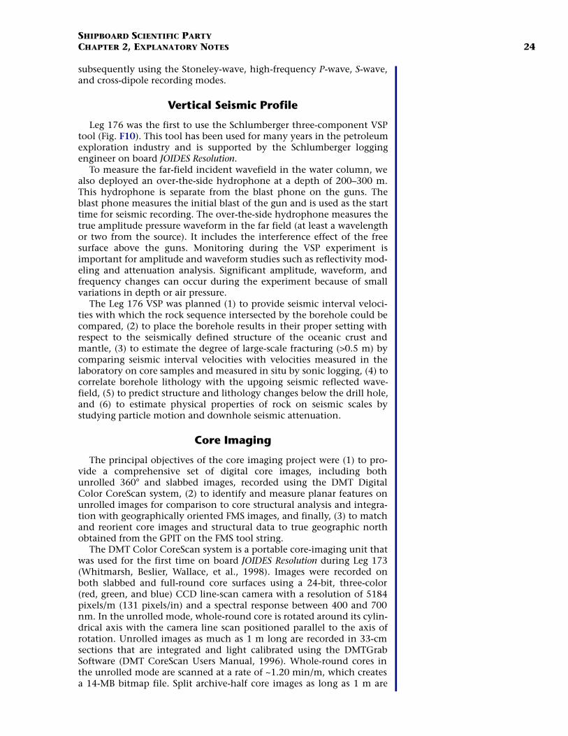
SHIPBOARD SCIENTIFIC PARTYCHAPTER 2, EXPLANATORY NOTES 24
subsequently using the Stoneley-wave, high-frequency P-wave, S-wave,and cross-dipole recording modes.
Vertical Seismic Profile
Leg 176 was the first to use the Schlumberger three-component VSPtool (Fig. F10). This tool has been used for many years in the petroleumexploration industry and is supported by the Schlumberger loggingengineer on board JOIDES Resolution.
To measure the far-field incident wavefield in the water column, wealso deployed an over-the-side hydrophone at a depth of 200–300 m.This hydrophone is separate from the blast phone on the guns. Theblast phone measures the initial blast of the gun and is used as the starttime for seismic recording. The over-the-side hydrophone measures thetrue amplitude pressure waveform in the far field (at least a wavelengthor two from the source). It includes the interference effect of the freesurface above the guns. Monitoring during the VSP experiment isimportant for amplitude and waveform studies such as reflectivity mod-eling and attenuation analysis. Significant amplitude, waveform, andfrequency changes can occur during the experiment because of smallvariations in depth or air pressure.
The Leg 176 VSP was planned (1) to provide seismic interval veloci-ties with which the rock sequence intersected by the borehole could becompared, (2) to place the borehole results in their proper setting withrespect to the seismically defined structure of the oceanic crust andmantle, (3) to estimate the degree of large-scale fracturing (>0.5 m) bycomparing seismic interval velocities with velocities measured in thelaboratory on core samples and measured in situ by sonic logging, (4) tocorrelate borehole lithology with the upgoing seismic reflected wave-field, (5) to predict structure and lithology changes below the drill hole,and (6) to estimate physical properties of rock on seismic scales bystudying particle motion and downhole seismic attenuation.
Core Imaging
The principal objectives of the core imaging project were (1) to pro-vide a comprehensive set of digital core images, including bothunrolled 360° and slabbed images, recorded using the DMT DigitalColor CoreScan system, (2) to identify and measure planar features onunrolled images for comparison to core structural analysis and integra-tion with geographically oriented FMS images, and finally, (3) to matchand reorient core images and structural data to true geographic northobtained from the GPIT on the FMS tool string.
The DMT Color CoreScan system is a portable core-imaging unit thatwas used for the first time on board JOIDES Resolution during Leg 173(Whitmarsh, Beslier, Wallace, et al., 1998). Images were recorded onboth slabbed and full-round core surfaces using a 24-bit, three-color(red, green, and blue) CCD line-scan camera with a resolution of 5184pixels/m (131 pixels/in) and a spectral response between 400 and 700nm. In the unrolled mode, whole-round core is rotated around its cylin-drical axis with the camera line scan positioned parallel to the axis ofrotation. Unrolled images as much as 1 m long are recorded in 33-cmsections that are integrated and light calibrated using the DMTGrabSoftware (DMT CoreScan Users Manual, 1996). Whole-round cores inthe unrolled mode are scanned at a rate of ~1.20 min/m, which createsa 14-MB bitmap file. Split archive-half core images as long as 1 m are

SHIPBOARD SCIENTIFIC PARTYCHAPTER 2, EXPLANATORY NOTES 25
recorded in slabbed mode with the camera line scan traveling perpen-dicular to the vertical core axis. Scanning 1 m of split core takes ~45 sand creates a 10-MB bitmap file.
During Leg 176, all cores were scanned in the unrolled mode withthe exception of those pieces that were not fully cylindrical and inter-vals of drilling breccia. Whole-round cores were scanned after the corewas run through the MST. A vertical line marked on the core with a redgrease pencil aided initial reorientation of the images back to the ODPreference frame. Unrolled images were obtained on contiguous corepieces whenever possible. The lengths of whole-round pieces unsuitablefor scanning were measured so the allowance could be made for themwhen images were integrated into core barrel lengths using the DMTSoftware CoreLog (DMT CoreScan Users Manual, 1996). Initial struc-tural analysis was performed; however, the majority of the structuralanalysis and core reorientation work was done after the cruise. Duringour sail to Hole 735B, split core (slabbed) images of the archive-halfwere obtained from the bottommost 50 m of the hole cored during Leg118. Selected images of the working half were also obtained from newcores during Leg 176.

SHIPBOARD SCIENTIFIC PARTYCHAPTER 2, EXPLANATORY NOTES 26
REFERENCES
Balch, A.H., and Lee, M.W. (Eds.), 1984. Vertical Seismic Profiling: Techniques, Applica-tions, and Case Histories: Boston (Int. Human Resour. Develop. Corp.).
Becker, K., Malone, M., et al., 1998. Proc. ODP, Init. Repts., 174B: College Station, TX(Ocean Drilling Program).
Blum, P., 1997. Physical Properties Handbook: a Guide to the Shipboard Measure-ments of Physical Properties of Deep-Sea cores. ODP Tech. Note, 26. College Station,TX (Ocean Drilling Program).
Bolmer, S.T., Buffler, R.T., Hoskins, H., Stephen, R.A., and Swift, S.A., 1992. Verticalseismic profile at Site 765 and seismic reflectors in the Argo Abyssal Plain. In Grad-stein, F.M., Ludden, J.N., et al., Proc. ODP, Sci. Results, 123: College Station, TX(Ocean Drilling Program), 583–600.
Bouchez, J.L., et al., 1992. Submagmatic microfractures in granite. Geology, 20:456–459.
Boyce, R.E., 1976. Definitions and laboratory techniques of compressional soundvelocity parameters and wet-water content, wet-bulk density, and porosity parame-ters by gravimetric and gamma-ray attenuation techniques. In Schlanger, S.O.,Jackson, E.D., et al., Init. Repts. DSDP, 33: Washington (U.S. Govt. Printing Office),931–958.
Cannat, M., Mével, C., and Stakes, D., 1991. Normal ductile shear zones at an oceanicspreading ridge: tectonic evolution of Site 735 gabbros (southwest Indian Ocean).In Von Herzen, R.P., Robinson, P.T., et al., Proc. ODP, Sci. Results, 118: College Sta-tion, TX (Ocean Drilling Program), 415–429.
Christie, P.A.F., Hughes, V.J., and Kennett, B.L.N., 1983. Velocity filtering of seismicreflection data. First Break, 1:9–24.
Dick, H.J.B., Meyer, P.S., Bloomer, S., Kirby, S., Stakes, D., and Mawer, C., 1991a.Lithostratigraphic evolution of an in-situ section of oceanic Layer 3. In VonHerzen, R.P., Robinson, P.T., et al., Proc. ODP, Sci. Results, 118: College Station, TX(Ocean Drilling Program), 439–538.
Dick, H.J.B., Schouten, H., Meyer, P.S., Gallo, D.G., Bergh, H., Tyce, R., Patriat, P.,Johnson, K.T.M., Snow, J., and Fisher, A., 1991b. Tectonic evolution of the AtlantisII Fracture Zone. In Von Herzen, R.P., Robinson, P.T., et al., Proc. ODP, Sci. Results,118: College Station, TX (Ocean Drilling Program), 359–398.
DMT-GeoTec/Geo-Engineering, 1996. DMT Color CoreScan Users Manual. Acquisitionand Evaluation Software.
Duennebier, F.K., Lienert, B., Cessaro, R., Anderson, P., and Mallick, S., 1987. Con-trolled-source seismic experiment at Hole 581C. In Duennebier, F.K., Stephen, R., etal., Init. Repts. DSDP, 88: Washington (U.S. Govt. Printing Office), 105–125.
Eberli, G.P., Swart, P.K., Malone, M.J., et al., 1997. Proc. ODP, Init. Repts., 166: CollegeStation, TX (Ocean Drilling Program).
Gal’perin, E.I., 1974. Vertical Seismic Profiling. Spec. Publ.—Soc. Explor. Geophys., 12.Gerland, S., and Villinger, H., 1995. Nondestructive density determination on marine
sediment cores from gamma-ray attenuation measurements. Geo-Mar. Lett.,15:111–118
Goldberg, D., 1997. The role of downhole measurements in marine geology and geo-physics. Rev. Geophys., 315–342.
Hardage, B.A., 1983. Vertical Seismic Profiling: Part A, Principles: London (GeophysicalPress).
Hirth, G., and Kohlstedt, D.L., 1995. Experimental constraints on the dynamics ofthe partially molten upper mantle: deformation in the diffusion creep regime. J.Geophys. Res, 100:1981–2001.
Hoppie, B.W., Blum, P., and the Shipboard Scientific Party, 1994. Natural gamma-raymeasurements on ODP cores: introduction to procedures with examples from Leg

SHIPBOARD SCIENTIFIC PARTYCHAPTER 2, EXPLANATORY NOTES 27
150. In Mountain, G.S., Miller, K.G., Blum, P., et al., Proc. ODP, Init. Repts., 150: Col-lege Station, TX (Ocean Drilling Program), 51–59.
Kommedal, J.H., and Tjøstheim, B.A., 1989. A study of different methods of wavefieldseparation for application to VSP data. Geophys. Prospect., 37:117–142.
Le Maitre, R.W., 1989. A Classification of Igneous Rocks and Glossary of Terms: Oxford(IUGS, Blackwell).
Means, W.D., and Park, Y., 1994. New experimental approach to understanding igne-ous texture. Geology, 22:323–326.
Mons, R., and Barbour, K., 1981. Vertical seismic profiling. Schlumberger WirelineAtlantic-Marketing Geophys., SMP-1108.
Nicolas, A., and Ildefonse, B., 1996. Flow mechanisms and viscosity in basalticmagma chambers. Geophys. Res. Lett., 23:2013–2016.
Rider, M., 1996. The Geological Interpretation of Well Logs: Caithness (Whittles Publish-ing).
Ross, W.S., and Shaw, P.M., 1987. Vertical seismic profile reflectivity: ups over downs.Geophysics, 52:1149–1154.
Rutledge, J.T., and Winkler, H., 1989. Attenuation measurements from vertical seis-mic profile data: Leg 104, Site 642. In Eldholm, O., Thiede, J., Taylor, E., et al., Proc.ODP, Sci. Results, 104: College Station, TX (Ocean Drilling Program), 965–972.
Schlumberger, 1995. DSI—Dipole Sonic Imager: (Schlumberger Wireline and Testing),SMP-5128.
Serra, O., 1984. Fundamentals of Well-Log Interpretation (Vol. 1): The Acquisition of Log-ging Data: Dev. Pet. Sci., 15A: Amsterdam (Elsevier).
————, 1989. Formation MicroScanner Image Interpretation: Houston (SchlumbergerEduc. Services), SMP-7028.
————, 1986. Fundamentals of Well-Log Interpretation (Vol. 2): The Interpretation ofLogging Data. Dev. Pet. Sci., 15B.
Shafer, H.N.S., 1996. The determination of iron(II) oxide in silicate and refractorymaterials. Part II. The Analyst, 91:755–762.
Shipboard Scientific Party, 1989. Site 735. In Robinson, P.T., Von Herzen, R., et al.,Proc. ODP, Init. Repts., 118: College Station, TX (Ocean Drilling Program), 89–222.
————, 1991. Explanatory notes. In Taira, A., Hill, I., Firth, J.V., et al., Proc. ODP,Init. Repts., 131: College Station, TX (Ocean Drilling Program), 25–60.
————, 1992. Explanatory notes. In Dick, H.J.B., Erzinger, J., Stokking, L.B., et al.,Proc. ODP, Init. Repts., 140: College Station, TX (Ocean Drilling Program), 5–33.
————, 1993. Explanatory notes. In Gillis, K., Mével, C., Allan, J., et al., Proc. ODP,Init. Repts., 147: College Station, TX (Ocean Drilling Program), 15–42.
————, 1995a. Explanatory notes. In Cannat, M., Karson, J.A., Miller, D.J., et al.,Proc. ODP, Init. Repts., 153: College Station, TX (Ocean Drilling Program), 15–42.
————, 1995b. Explanatory notes. In Humphris, S.E., Herzig, P.M., Miller, D.J., etal., Proc. ODP, Init Repts., 158: College Station, TX (Ocean Drilling Program),37–53.
————, 1995c. Explanatory notes. In Shipley, T.H., Ogawa, Y., Blum, P., et al., Proc.ODP, Init. Repts., 156: College Station, TX (Ocean Drilling Program), 39–68.
————, 1998. Explanatory notes. In Fouquet, Y., Zierenberg, R., Miller, D.J., et al.,Proc. ODP, Init. Repts., 169: College Station, TX (Ocean Drilling Program), 17–32.
Stephen, R.A., 1979. The oblique seismic experiment in oceanic crust: experimentand technique. Mar. Geophys. Res., 4:213–226.
Streckeisen, A., 1974. Classification and nomenclature of plutonic rocks. Geol. Rund-sch., 63:773–786.
Swift, S.A., Hoskins, H., and Stephen, R.A., 1991. Seismic stratigraphy in a transverseridge, Atlantis II Fracture Zone. In Von Herzen, R.P., Robinson, P.T., et al., Proc.ODP, Sci. Results, 118: College Station, TX (Ocean Drilling Program), 219–226.
Swift, S.A., and Stephen, R.A., 1992. How much gabbro is in ocean seismic layer 3?Geophys. Res. Lett., 19:1871–1874.
Whitmarsh, R.B., Beslier, M.-O., Wallace, P.J., et al., 1998. Proc. ODP, Init. Repts., 173:College Station, TX (Ocean Drilling Program).

SHIPBOARD SCIENTIFIC PARTYCHAPTER 2, EXPLANATORY NOTES 28
Figure F1. Diagram illustrating terms used in the discussion of coring operations and core recovery.
Sea level
SeafloorSub-bottom top
CO
RE
1C
OR
E 2
CO
RE
3C
OR
E 6
CO
RE
4C
OR
E 5
a
b
c
d
e
f
Drilled butnot cored
Pen
etra
tion
Recoveredmaterial
Sub-bottom bottom
Dual elevator stool (DES)
BOTTOM FELT- Distancefrom DES to seafloor
TOTAL DEPTH- Distancefrom DES to bottom of hole(sub-bottom bottom)
PENETRATION- Distancefrom seafloor to bottom ofhole (sub-bottom bottom)
NUMBER OF CORES-Total of all cores recorded,including cores with norecovery
TOTAL LENGTH OFCORED SECTION-Distance from seafloor tobottom of hole less drilledbut not cored intervals
TOTAL CORE RECOVERED-For this diagram: Total additivelength of a, b, c, d, e, f
CORE RECOVERY %- Equal toTOTAL CORE RECOVEREDdivided by TOTAL LENGTH OFCORED SECTION, multiplied by100
Drill pipe measurement (DPM)

SHIPBOARD SCIENTIFIC PARTYCHAPTER 2, EXPLANATORY NOTES 29
Figure F2. Diagram illustrating hard-rock core division procedures.
Sectionnumber
1
2
3
4
5
6
7
1
2
3
4
void
Sectionnumber
Sectionnumber
FULLRECOVERY
PARTIALRECOVERY
PARTIALRECOVERY
Cor
ed in
terv
al =
9.5
m
6
5
void
void
4
3
2
1
emptyliner
emptyliner
emptyliner
Top
Top
Top
Cor
ed in
terv
al =
9.5
m
Cor
ed in
terv
al =
9.5
m

SHIPBOARD SCIENTIFIC PARTYCHAPTER 2, EXPLANATORY NOTES 30
Figure F3. This figure illustrates core curation procedures for hard rocks. Letters designating pieces as re-moved from core barrel are for illustrative purposes only. Pieces A, B, C, D, E, and F become interval XXX-YYYZ-1R-1, Piece 1 to Piece 6 (where XXX is the leg, YYY is the site, and Z is the hole designator). Becausepieces G and H can be reoriented to fit along a fracture, they are curated as a single piece. In this case, thereassembled single piece is too long to fit in the bottom of Section 1R-1, so it is shunted to the top of Section1R-2 and curated as interval XXX-YYYZ-1R-2, (Pieces 1A and 1B). Similarly, pieces L and M are too long tofit in the bottom of Section 1R-2 after realignment and are shunted to the top of Section 1R-3. Spacers be-tween pieces also artificially add length to the core when measured for archiving and curation. For exam-ple, pieces L and M represent an interval from 2.17 to 2.63 m down from the top of the core as removedfrom the core barrel, but are archived as interval XXX-YYYZ-1R-3 (Pieces 1A and 1B, 0.0–46.0 cm).
1A
1B
2
3
4
1R-2
Pieces as removed from core barrel
CU
RA
TE
D L
EN
GT
H 2
.75
m
CORE 1R
H
I
1
2
3
4
5
6
1R-1
2
1R-3
A
B
C
D
E
F
G
J
K
L
M
N
Butylate liner
Spacers
Section Section Section
SEC
TIO
N L
EN
GT
H 1
.5 m
Emptyliner
1A
1B

SHIPBOARD SCIENTIFIC PARTYCHAPTER 2, EXPLANATORY NOTES 31
Figure F4. Example of hard-rock visual core description (HRVCD) form.
CORE/SECTION
176-735B-89R-1
100
150
140
130
120
110
90
80
70
60
50
40
30
20
10
0
H
M
H
M
H
PMAG
1
2
3
4A
4B
5
6
495
496
Interval 495: TROCTOLITIC GABBRODepth in Depth
Interval Location: Core Section Section Piece mbsfUpper contact: 88 1 4 1 500.04Lower contact: 89 1 125 6 502.30Thickness: 2.29 m
Grain Size:Mode Max Min Size Shape/Habit
Plagioclase 60 10 3 coarse tabular /subhedral
Clinopyroxene 35 100 2 coarse equant/oikocrysticanhedral
Olivine 10 25 3 coarse amoeboidal/anhedral
Opaques 0.5Total 105.5**Major phases estimated to ± 5%Modal name (calculated): Olivine GabbroGrain Size: Medium
Type DistributionStructure: intergranular evenly distributedFabric N/A N/AComments: Olivine heavily altered in zones next to fractures. Someclinopyroxene elongated. Clinopyroxene mode variable (5%-40%). Locallygranular. Pegmatitic clinopyroxene from 32-40 cm. Poikilitic clinopyroxenefrom 72-76 cm.
Alteration:Dark green amphibole:
Total Percent: <15Mode of occurrence: Mainly after clinopyroxene, partly after olivine.Comments: As alteration rims, secondary plagioclase.
Secondary plagioclase:Total Percent: <20Mode of occurrence: Replacing primary plagioclase.Comments: Irregularly distributed.
Talc, oxides and (chlorite):Total Percent: <2Mode of occurrence: Replacing olivine.Comments: As mixures in the crystal crack network and aroundcrystals (green amphinbole and dark blue chlorite).
Oxyhydroxides and smectites:Total Percent: <2Mode of occurrence: Replacing olivine relics.Comments: Mixture of orange-red clays and carbonates with earlymetamorphic assemblages.
Carbonates:Total Percent: <1Mode of occurrence: In veins and replacing olivine.Comments: Weathering of olivine is related to carbonate veinformation.
Background Alteration:Degree of alteration: moderate (30%-40%). Olivine is largely replaced byamphibole, talc, and oxides (ca. 80%). Clinopyroxene is rimmed by amphibole(ca. 5%). Plagioclase is partly recrystallized (5%). Superimposed to this high-temperature alteration is weathering of olivine relicts along cracks and carbonateveins.
Vein/Fracture Filling:Amphibole veins in Pieces 1 and 4A are 7 cm in length, 0.5-0.6 mm wide.Carbonate veins in Pieces 3,4A, 5, and 6 are 4-6 cm in length, 0.5-1.0 mm wideand are associated with pervasive oxidation of olivine.
Structures:Mf>V; Mf>JThis section does not contain plastic deformation. Igneous texture can beobserved along the complete section. Magmatic fabric is null or weak (0,1).One narrow cataclastic zone (<1cm) overprints the magmatic texture at the topof the section (Piece 1). A few veins and joints. Arrays of subvertical cracks ormicroveins are often visible in big plagioclases and pyroxenes.
Interval 496: See next section
1
2
3
4
5
Gra
phic
Rep
rese
ntat
ion
Pie
ce n
umbe
r
Mea
sure
men
t ID
Str
uctu
re
Lith
olog
ic u
nit
Shi
pboa
rd s
tudi
es
Orie
nta
tion
Str
uct
ure
Met
amor
phis
m
Vei
ns
Gra
phic
Lith
olog
y
cm

SHIPBOARD SCIENTIFIC PARTYCHAPTER 2, EXPLANATORY NOTES 32
Figure F5. Graphic lithology patterns used during Leg 176.
Gabbro
Oxide gabbro
Olivine gabbro
Oxide olivine gabbro
Gabbronorite
Oxide gabbronorite
Microgabbro
Oxide troctolite
Diorite
Clinopyroxenite
Troctolite

SHIPBOARD SCIENTIFIC PARTYCHAPTER 2, EXPLANATORY NOTES 33
Figure F6. Comparison of lithostratigraphic intervals defined during Leg 176 with those defined by Dicket al. (1991a) for the core recovered from 450 to 500 mbsf during Leg 118.
438a
439439
440 440
450
452
454
456
458
460
462
464
466
468
470
472
474
442 442
444 444
446
447
448 448
451
449451451a
452452
452a
452c
453
453
457
457456d
455456a
476
478
480
482
484
486
488
490
492
494
496
498
500
461
460
460b
462462
465a
466
469a
469b
471
473a
474
474
471
470
469
466
467
475 475
476 476
477
478
482
476a
476b
477
480
482
492
485
486
487
484a484b
487
491a
493
Depth(mbsf)
Leg 176intervals
Leg 118intervals
Depth(mbsf)
Leg 176intervals
Leg 118intervals
447
463 463
446

SHIPBOARD SCIENTIFIC PARTYCHAPTER 2, EXPLANATORY NOTES 34
Figure F7. Classification of ultramafic and gabbroic rocks composed of olivine, clinopyroxene,orthopyroxene, and plagioclase (after Streckeisen, 1974).
olivineplagioclase plagioclase
plagioclase
orthopyroxeneclin
opyr
oxen
e
dunitetroctolite troctolite
gabb
ro
wehrlite
harz
burg
ite
norite
websterite
gabbronoritega
bbro norite
olivinewebsterite
olivine gabbro olivine noritelherzolite
clinopyroxenite
orthopyroxenite
anorthositeanorthosite
anorthosite
oliv
ine
orth
opyr
oxen
ite
olivine
clinopyroxenite
90
5
40

SHIPBOARD SCIENTIFIC PARTYCHAPTER 2, EXPLANATORY NOTES 35
Figure F8. Classification of silica saturated or oversaturated plutonic rocks, based on quartz, plagioclase,and alkali feldspar (Streckeisen, 1974).
granite
granodiorite
tonalite
quartz diorite
dioritemonzodioritemonzonite
quartzmonzodiorite
quartzmonzonite
syenite
quartz syenite
alkali feldspar quartz syenite
alkali feldspar syenite
alkalifeldspar plagioclase10 35 65 90
5
20
60
alka
li fe
ldsp
ar g
rani
te
quartz
granitoids

SHIPBOARD SCIENTIFIC PARTYCHAPTER 2, EXPLANATORY NOTES 36
Figure F9. Core flow for physical properties measurements in hard-rock boreholes.
Core into lab
Core preparation& equilibration
Core is runthrough MST
Core splitting
Thermal conductivity
measurements
Apply thermaljoint compound
Archive half core
Working half core
Check andupload into
JANUS
Sampling party
Minicores cut
Resaturateminicore
in vacuum
Wet mass
Dry in oven
Drymass
Dry densityin pycnometer
Smooth ends ofminicore and
check they areparallel
Check andupload into
JANUS
Check andupload into
JANUS
P-wave velocityCheck andupload into
JANUS
1-2 HOURS
1 HOUR +
DAILY
24 HOURS
24 HOURS
ITALICS = Time lags
BOLD = PHYSICAL PROPERTY TEAM ACTIONS
Smooth surfaceand clean
ultrasonically Teflon wrap sample
Measureresistivity
Check andupload into
JANUS
Emerse in basinto equilibrate &resaturate core

SHIPBOARD SCIENTIFIC PARTYCHAPTER 2, EXPLANATORY NOTES 37
Figure F10. Schematic diagram of the wireline logging tool strings deployed during Leg 176. (1) Modifiedtriple combo string deployed at the end of the cruise; (2) FMS/DSI combination; (3) resistivity (DLL) andgeneral purpose inclinometry tool (GPIT) combination; and (4) VSP tool.
Cablehead
Telemetry
NGT-C
DSI
(2)
Cablehead
Telemetry
HNGS
APS
HLDT
Caliper
(1)
NGT-C
DLL
GPIT
(3)
Cablehead
Telemetry
Bridle
VSP
(4)
MEST-C

SHIPBOARD SCIENTIFIC PARTYCHAPTER 2, EXPLANATORY NOTES 38
Figure F11. Schematic diagram of VSP geometry and record section illustrating how direct and reflectedarrivals differ with changes in receiver depth (modified after Mons and Barbour, 1981).
Time
1
2
3
4
5
Downgoingdirect wave
Downgoing multiple direct wave
Source
Seafloor
ReflectorReflected wave
Geophone position

SHIPBOARD SCIENTIFIC PARTYCHAPTER 2, EXPLANATORY NOTES 39
Table T1. X-ray fluorescence operating conditions.
Notes: All major elements measured using a rhodium X-ray tube operated at 30 kV and 80 mA. Trace ele-ments are measured using a rhodium X-ray tube operated at 60 kV and 50 mA. Detector: FPC = flowproportional counter (P10 gas); Scint = NaI Scintillation counter. Detection limits in weight percent formajor oxides, parts per million for trace elements.
Oxide orelement Line Crystal Detector Collimator
Peakangle(°2θ)
Backgroundoffset(°2θ)
Count timeon
peak(s)
Count timeon
background (s)
SiO2 Kα PET FPC Medium 109.21 40TiO2 Kα LIF200 FPC Fine 86.14 40Al2O3 Kα PET FPC Medium 145.12 100Fe2O3 Kα LIF200 FPC Fine 57.52 40MnO Kα LIF200 FPC Fine 62.97 100MgO Kα TLAP FPC Medium 45.17 ±0.80 150 150CaO Kα LIF200 FPC Medium 113.09 40Na2O Kα TLAP FPC Medium 54.10 –1.20 150 150K2O Kα LIF200 FPC Medium 136.69 100P2O5 Kα GE111 FPC Medium 141.04 100
Rh Kα Compton LIF200 Scint Fine 18.58 60Nb Kα LIF200 Scint Fine 21.40 +0.35 200 100Zr Kα LIF200 Scint Fine 22.55 –0.35 100 50Y Kα LIF200 Scint Fine 23.80 –0.40 100 50Sr Kα LIF200 Scint Fine 25.15 –0.40 100 50Rb Kα LIF200 Scint Fine 26.62 –0.60 100 50Zn Kα LIF200 Scint Medium 41.81 –0.55 100 50Cu Kα LIF200 Scint Fine 45.03 –0.55 100 50Ni Kα LIF200 Scint Medium 48.67 –0.60 100 50Cr Kα LIF200 FPC Fine 69.35 –0.50 100 50V Kα LIF220 FPC Fine 123.06 –0.50 100 50

SHIPBOARD SCIENTIFIC PARTYCHAPTER 2, EXPLANATORY NOTES 40
Table T2. Deformation intensity scales.
Category: 0 1 2 3 4 5
Magmatic Isotropic: no shape fabric
Weak shape fabric Moderate shape fabric
Strong shape fabric
Crystal plastic Undeformed Weakly foliated Strongly foliated Porphyroclastic (proto)mylonite
Mylonite Ultramylonite
Cataclastic Undeformed Minor fracturing: no significant grain-size reduction
Moderate fracturing: no significant grain-size reduction
Dense anastomosing fracturing and incipient breccia(<20% matrix)
Well-developed fault brecciation; rotation of clasts (20% to 70% matrix)
Cataclasite(>70% matrix)
Joints Unfractured Minor fracturing (≤1 per 10 cm)
(1 to 5 per 10 cm) (>5 per 10 cm)
Veins No veins Occasional veins(= filled fractures)(≤1 per 10 cm)
Moderate veining (1 to 5 per 10 cm)
Intense vein networks (>5 per 10 cm)

SHIPBOARD SCIENTIFIC PARTYCHAPTER 2, EXPLANATORY NOTES 41
Table T3. Checklist used for spreadsheet comments associatedwith each structural identifier.
The following is a checklist of structural characteristics that were searched for in macroscopic core samples. These characteristics supplement the information required by the spreadsheet and were noted in the comments section of the spreadsheet. The abbreviations for these features were used to document crosscutting relationships (where > indicates “older than”) on the structure section of the VCDs.
Subhorizontal microcracks (Shm) Drilling-induced fractures
Join ts (J) Joint density Orientation Plume structures on joint surface
Veins (V) Orientation of veins and vein-array boundaries Magnitude and nature of offset Density of vein network Array characteristicsSense of shearAngle between new vein segments and array boundary (measure of array dilatation) Internal structure of fibers Crack-seal structures and number of vein-opening events Wall-rock alteration and shape Vein terminations (splayed or tapered) Vein mineralogy
Faults (F) Fault-zone thickness, orientation and density Movement sense (r,n,d,s), reverse, normal, dextral sinistral Intensity of cataclastic fabric (Cf) Matrix material (gouge or secondary minerals) Overprinting of pre-existing fabric Semi-brittle
Breccias (B) Hydrothermal (Bh), magmatic (Bm) or cataclastic (Bc) Clast size and shape, matrix composition, relative proportions
Cleavages (C) Style of cleavage (e.g., crenulation [Cc], spaced [Cs]) Spacing or wavelength Angle between cleavage and earlier fabrics, noting directions of larger-scale fold closures
Folds (Fo) Inter-limb angle Estimate of hinge curvature (e.g., kink vs. round) Asymmetry of hingeline relative to other fabrics (e.g., stretching lineations, etc.) other geometrical aspects preserved in core (e.g., wavelength, amplitude, etc.) Number of folds, if more than one
Crystal-Plastic Fabrics (Pf) Intensity of fabric Intensity of fabric in retrograde assemblage Orientation of foliation (Sp) and lineation (Lp) L-, LS- and S-tectonite Shear sense indicators: block-rotated porphyroclasts, asymmetric augen, SC fabrics, discrete
shear bands, mica-fish, and tension-gash arrays (r,n,d,s), reverse, normal, dextral sinistral Mineralogical segregation or banding
Magmatic Fabrics (Mf) Intensity and orientation of foliations (Sm) and lineations (Lm) Minerals that define the shape and/or crystallographic preferred orientations Angle between crystallographic and shape fabrics Orientation of subfabrics
Compositional Layering (Cl)/Gradational Boundaries (Gb) Type of layering (e.g., sedimentary, igneous cumulate, alteration, etc.) Orientation, thickness, and density of layers
Igneous Contacts (Ic) Orientation and density Concordant or discordant
Crosscutting Relationships Intrusive relationships, relative chronology of the different fabrics Angle between compositional layering and magmatic or crystal-plastic fabric

SHIPBOARD SCIENTIFIC PARTYCHAPTER 2, EXPLANATORY NOTES 42
Table T4. Textural types characterized by specific microstructural styles for gabbroic rocks.
Textural group Plagioclase Olivine Pyroxene Physical state
1 No or minor crystal-plastic deformation microstructures (e.g., deformation twins, undulose extinction)
No deformation microstructures ± local undulose extinction and/or local subgrain development
No deformation microstructures Primarily magmatic
a Random shape orientationb Preferred shape orientation
2 <30% fine-grained recrystallized matrix; deformation twins and subgrain boundaries may be present
Common subgrain boundaries and undulose extinction
No deformation microstructures ± minor crystal-plastic deformation microstructures
Crystal-plastic ± magmatic
3 >30% recrystallized matrix; deformation twins, subgrain boundaries, and undulose extinction common; moderate shape preferred orientation; strong crystallographic preferred orientation
Elongated aggregates of neoblasts Kinked grains; common to extensive recrystallization
Crystal-plastic
4 Strongly bimodal grain size distribution; localized fine-grained neoblasts, polygonal neoblasts, sutured neoblasts
Closely spaced subgrain boundaries; pervasive undulose extinction extensive neoblasts
Bent/kinked porphyroclasts; localized recrystallization
Crystal-plastic
5 Common intracrystalline microfractures associated with very fine-grained neoblasts; extensive kinked and deformation twinned grains; pervasive undulose extinction; may contain hydrothermal alteration mineral assemblages
Same as plagioclase Same as plagioclase Semibrittle
6 Intra/intercrystalline microfractures and cataclastic bands; extensive kinked and deformation twinned grains; pervasive undulose extinction
Same as plagioclase Same as plagioclase Brittle/cataclastic
Related Documents


