2 Earnings Inequality and Educational Mobility in Brazil over Two Decades Denis Cogneau and Je ´re ´mie Gignoux 2.1 Introduction Brazilian society, from a number of points of view, is one of the most inegalitarian in the world, and special attention has consequently been paid to it for a long time (Fishlow 1972). The South American and Caribbean societies are particularly inegalitarian. This characteristic has now been related to the institutions left over from the colonial pe- riod (Sokoloff and Engerman 2000). The level of inequality in Brazil is much greater even than the average on the subcontinent with, for example, a Gini index one-third higher than Argentina (UN/WIDER data), and at the same level as in South Africa (Lam 1999). The colonial legacy probably weighs heavy from this point of view, since Brazil was the region’s main slave country. Correlatively, the Brazilian economy and society display an extremely high degree of dualism, visible both in the education system (private/state) and on the labor market (official/unofficial). Brazil is also among the countries with the lowest intergenerational educational mobility and equality of social and eco- nomic opportunities in the world (Dunn 2007). A series of nationally representative annual surveys based on large samples (Pesquisa Nacional por Amostra de Domicilios, or PNAD, 1976–1996) provides a fairly accurate observation of the change in inequality in Brazil over nearly thirty years. These data show that income inequality remained remarkably stable, whether the gaps were in individual earnings or household standards of living. The 1976, 1982, 1988, and 1996 PNAD surveys also include certain information on individuals’ social origin. Sociologists have used these data to pro- duce the first quantitative analyses of intergenerational social mobility in Brazil (Pastore 1982, Pastore and Valle Silva 2000, Picanc ¸o 2004). Economists have also recently looked into the impact of family origins

Welcome message from author
This document is posted to help you gain knowledge. Please leave a comment to let me know what you think about it! Share it to your friends and learn new things together.
Transcript

2 Earnings Inequality and Educational Mobility inBrazil over Two Decades
Denis Cogneau and Jeremie Gignoux
2.1 Introduction
Brazilian society, from a number of points of view, is one of the most
inegalitarian in the world, and special attention has consequently been
paid to it for a long time (Fishlow 1972). The South American and
Caribbean societies are particularly inegalitarian. This characteristic
has now been related to the institutions left over from the colonial pe-
riod (Sokoloff and Engerman 2000). The level of inequality in Brazil
is much greater even than the average on the subcontinent with, for
example, a Gini index one-third higher than Argentina (UN/WIDER
data), and at the same level as in South Africa (Lam 1999). The colonial
legacy probably weighs heavy from this point of view, since Brazil was
the region’s main slave country. Correlatively, the Brazilian economy
and society display an extremely high degree of dualism, visible both
in the education system (private/state) and on the labor market
(official/unofficial). Brazil is also among the countries with the lowest
intergenerational educational mobility and equality of social and eco-
nomic opportunities in the world (Dunn 2007).
A series of nationally representative annual surveys based on large
samples (Pesquisa Nacional por Amostra de Domicilios, or PNAD,
1976–1996) provides a fairly accurate observation of the change in
inequality in Brazil over nearly thirty years. These data show that
income inequality remained remarkably stable, whether the gaps were
in individual earnings or household standards of living. The 1976,
1982, 1988, and 1996 PNAD surveys also include certain information
on individuals’ social origin. Sociologists have used these data to pro-
duce the first quantitative analyses of intergenerational social mobility
in Brazil (Pastore 1982, Pastore and Valle Silva 2000, Picanco 2004).
Economists have also recently looked into the impact of family origins

and inequality of educational and labor market opportunities (Lam
and Schoeni 1993; Arias, Yamada, and Tejerina 2002; Andrade et al.
2003; Ferreira and Veloso 2006; Bourguignon, Ferreira, and Menendez
2007; Dunn 2007). All these studies emphasize that inequality in Brazil
comes with a high degree of intergenerational transmission of educa-
tion, occupational status, or income. One of the main questions put in
these papers concerns the contribution of education to the reduction of
economic inequality. Most argue that education is one prominent chan-
nel through which parental resources, and in particular parental edu-
cation, influence the labor market position and the living standard of
individuals.
This analytic question ties in with a contemporary political issue,
since Brazil set up extensive means-based transfer programs in 1999
that were conditional on sending children to school (Bolsa Escola) and
stopping child labor (PETI). These programs have now been combined
into a single program called Bolsa Familia and are reaching cruising
speed with widespread coverage. However, it is not easy to evaluate
the impact of these programs since, unlike the Mexican Progresa pro-
gram, no randomly allocated pilot setup has been implemented. An
ex-ante evaluation of the Bolsa Escola program using a structural
microeconometric model finds that the transfers have a significantly
positive, albeit modest, impact on school enrollment and child labor.
Hence they only have a marginal impact on income inequality and
poverty (Bourguignon, Ferreira, and Leite 2003). An ex-post evaluation
of the program is underway using data from the PNAD surveys,
which identify the recipient households (Leite 2006).
Whatever the impact of these programs on the education of the most
underprivileged children, a second question arises as to the long-run
impact of a decrease in educational inequality on the distribution of
income in Brazil. As regards the reduction of income inequality, the
hopes raised by the huge surge in the average level of education have
not yet been realized, contrary to optimistic forecasts by Lam and Lev-
ison (1991) (see Ferreira and Paes de Barros 2000 and 2004 on house-
hold income poverty). A recent paper by Bourguignon, Ferreira, and
Menendez (2007) applies microsimulation techniques to the 1996
PNAD survey to analyze the contribution of inequalities of educational
and income opportunity to the formation of inequality in an urban
environment. It concludes that the canceling out of inequality due to
social origin variables (race, region of birth, and parental education
and occupation) would reduce the Theil index of individual earnings
48 Denis Cogneau and Jeremie Gignoux
by more than one-fifth. The study’s authors deem these findings dis-
appointing since they only bring Brazil down to an average level of
inequality by Latin American standards and a level way above compa-
rable Asian countries. They however argue that this 20 percent share
should be considered as a lower bound. They also find that a large
part (55 to 75 percent) of the impact of factors of origin on individual
earnings is associated with parental schooling. Lastly, 70 percent of
this impact can be imputed to the direct effect of factors of origin on
earnings while the remaining 30 percent corresponds to the indirect ef-
fect of social origins going through education—that is, the equalization
of schooling opportunities.
This chapter addresses similar questions using a different set of data
and other econometric methods. The remainder of the introduction
provides a road map along with an overview of the main results.
The first section describes the data and the construction of the main
variables. We use four PNAD surveys from 1976, 1982, 1988, and 1996
to focus on individual earnings inequalities among men aged 40 to 49
and to conduct a historical decomposition of the evolution of inequal-
ities; in contrast, Bourguignon, Ferreira, and Menendez (2007) conduct
static microsimulations by cohorts on the 1996 survey.
The second section describes the evolution of two kinds of earnings
inequality over the 1976–1996 period: overall inequality in observed
earnings and inequality of opportunity. Alongside traditional indica-
tors of earnings inequality, we construct and calculate—for the first
time in the case of Brazil—inequality of opportunity indicators in
keeping with the axiomatics proposed by Roemer (1996 and 1998) and
by Van de Gaer (1993) and Van de Gaer, Schokkaert, and Martinez
(2001). Inequality of opportunity is defined as the amount of earnings
inequality that can be attributed to individuals’ social origins. We first
show that the two kinds of earnings inequality displayed a similar his-
torical path, including a peak in the late 1980s with the end of the dic-
tatorship (1985) and the height of the inflationary crisis (the Cruzado,
Bresser, Summer, and Collor Plans). All things considered, overall in-
equality rose slightly from the beginning to the end of the period,
while inequality of opportunity posted a slight drop.
A third section looks at educational inequality with the same lenses
as for earnings: overall inequality in education levels and inequality of
opportunity. It reveals that the average number of years spent in the
education system rose steadily for the generations born from 1927 to
1956, with a slight acceleration for the generations born in and after
Earnings Inequality, Educational Mobility in Brazil over Two Decades 49

the 1940s. Intergenerational educational transmission, defined as the
strength of the association between fathers’ and sons’ education, also
recorded a very slight downturn for these generations. The rise in sec-
ondary and higher education immediately following the war, meaning
the generations educated from 1945 to 1965, benefited mainly the chil-
dren of the upper classes. For the generations educated from 1955 to
1975, the expansion of primary schooling had more benefit for the chil-
dren of the underprivileged classes.
A fourth section then looks at the impact of these educational
changes on earnings inequalities evolution. Three factors of the evolu-
tion are considered: 1) changes in the distribution of education of
fathers and of sons; 2) changes in the pattern of mobility corresponding
to the transition matrix between them; and 3) the structure of returns
to parental education and own education. As an alternative to the
parametric microsimulation techniques, we propose a semiparametric
decomposition furnished by the log-linear model and nonparametric
reweighting techniques inspired by Di Nardo, Fortin, and Lemieux
(1996). We reveal that changes in the distribution of education levels
initially had an inegalitarian effect before becoming equalizing in the
late 1980s, for both kinds of earnings inequality. However, other fac-
tors, especially macroeconomic shocks, with soaring inflation and a
drop in the minimum wage in real terms, provoked a sharp rise in
earnings inequalities from 1982 to 1988. Yet this increase was virtually
absorbed in the 40–49-year-old age bracket from 1988 to 1996 due to
the expansion of primary education. Moreover, the change in the struc-
ture of earnings by education level and type of social origin had an
egalitarian effect mainly at the end of the period, in particular in the
form of a decrease in returns to education. Lastly, we determine that
the historical growth in intergenerational educational mobility for the
generations born from 1927 to 1956 was too small to play a significant
part in the developments observed. This explains the persisting in-
equality of economic opportunity at a high level.
A fifth and final section explores the potential for a reduction in eco-
nomic inequality stemming from an acceleration of intergenerational
educational mobility; that is, a mitigation of what Bourguignon, Fer-
reira, and Menendez (2007) call the ‘‘indirect effect’’ of parental edu-
cation on earnings. This kind of improvement indeed constitutes a
long-term target for the Bolsa Escola program. We confirm that the
bulk of the inequality of opportunity on the labor market can be
imputed to this factor; in contrast with Bourguignon, Ferreira, and
50 Denis Cogneau and Jeremie Gignoux

Menendez, we attribute an even larger share to this indirect effect, in
comparison with the direct impact of fathers’ education on earnings.
However, as found by Bourguignon, Ferreira, and Menendez, both
effects only play a modest role in overall inequality. We nevertheless
put forward that, in contrast with the historical decompositions or the
impact on inequality of opportunity, this last evaluation is highly sen-
sitive to earnings measurement errors.
2.2 Data
We use the data from four editions of the national survey of house-
holds (PNAD) conducted by the Brazilian Institute of Statistics (IBGE)
in 1976, 1982, 1988, and 1996. The PNAD surveys cover a large sample
since the data concern nearly 100,000 households every year. The sam-
ple is representative of the population of Brazil, but excludes the rural
areas in the northern region (the Amazon).1
These four editions contain information on the adults’ social origins,
collected for the head of household and his spouse.2 This concerns the
father’s level of education and occupation when the individual started
working.3 In addition, a question on migration provides information
on the individual’s place of birth (Federative Republic State)4 and the
questionnaire on demographic characteristics provides information on
the individual’s color. Overall, therefore, we use four data on social
origins.
We restrict the sample to men aged 40 to 49 and subsequently dis-
regard age effects on the assumption that such effects are negligible
within this group. We limit the sample to men declared as the head of
household or, more rarely, the spouse of the head (who combined rep-
resent 92 to 94 percent of this age bracket depending on the edition)
and to employed individuals (93 to 89 percent, with this proportion
decreasing over time) for whom information on social mobility, work-
ing hours, and earned income is provided. Our samples cover 2,860
observations in 1976; 18,833 in 1982; 11,304 in 1988; and 14,096 in 1996.
We construct an hourly earnings rate variable based on the informa-
tion on monthly incomes in the different economic activities, wage and
nonwage combined,5 and on the weekly hours worked in these activ-
ities.6 The incomes are discounted to September 2002 Brazilian reals
using the IBGE deflators derived from the INPC national consumer
price index. Ferreira, Lanjouw, and Neri (2003) posit that the PNAD
underestimates agricultural earnings due to the lack of information on
Earnings Inequality, Educational Mobility in Brazil over Two Decades 51

income in kind and production for own consumption, and overesti-
mates the production of family businesses due to the lack of informa-
tion on their expenditure on inputs. Overall, they deem that incomes
are underestimated in rural areas. This would appear to be borne out
by a comparison with the incomes measured by the 1996–1997 Pes-
quisa Sobre Padroes de Vida (PPV) living standards measurement
survey containing more information on these points. Despite these po-
tential measurement errors, we do not limit the sample to urban areas
as done by Bourguignon, Ferreira, and Menendez (2007). Analyzing
intergenerational mobility based on an urban subsample can result in
substantial selection biases. We believe that such biases are greater
than those caused by the underestimation of incomes in rural areas.
Disregarding spatial variations in purchasing power constitutes an-
other source of potential bias in the measurement of incomes. Ferreira,
Lanjouw, and Neri (2003) propose a series of regional deflators based
on data from the 1996 Pequisa de Orcamento Familiar (POF) house-
hold budget survey. We have tested these deflators in our empirical
analyses for this year and observed that the findings changed little.
We therefore do not correct these potential biases in the rest of this
work.
The variable used for the education level of the individuals in the
sample corresponds to the highest education level attained in numbers
of years after entry into primary school, which is normally at seven
years old.7 We use a discrete decomposition of this variable into nine
education levels (0, 1, 2, 3, 4, 5–7, 8, 9–11, and 12 or more years of
education).
We use two characterizations of the social origins of the individuals
in the sample. The first consists of four categorical variables. Variable
1 is a color variable coded into two categories, white for individuals
declared as being white or Asian and black for individuals declared as
being black, mixed race, or Indian. A birth region is variable 2, coded
into four categories designed so as to optimize both their sample size
and their discriminating power,8 covering respectively the individuals
born in (1) the Federal District and the state of Sao Paulo; (2) the states
of the southern region [excepting Rio Grande do Sul], center-western
region and west of the northern region; (3) the states of the south-
eastern region [excepting Sao Paulo], of the south of the northeastern
region [Alagoas, Bahia, and Sergipe], and Rio Grande do Sul; (4) the
states of the north of the northeastern region and east of the northern
region [Amapa and Para]). Father’s level of education is variable 3,
52 Denis Cogneau and Jeremie Gignoux

coded into four categories covering respectively the individuals whose
father (1) never went to school, (2) is literate or for whom the inter-
viewee is unable to give an answer, (3) completed one of the first four
years of primary education, and (4) completed at least the fifth year of
primary education). The fourth variable concerns the father’s occupa-
tion, and is coded into four categories covering respectively the indi-
viduals whose father was (1) a farmer; (2) employed in a traditional
industry, a domestic employee, or whose occupation is poorly defined
or for whom the interviewee is unable to give an answer; (3) employed
in a modern industry, an unincorporated entrepreneur, or employed in
a service sector; and (4) in a skilled profession, an employer, adminis-
trator, or manager. These four variables identify 128 groups of poten-
tial social origins.
The second characterization of social origins consists of a nine-
category classification based on the father’s level of education and oc-
cupation, covering the individuals whose father (1) never went to
school and was a farmer, (2) never went to school and had another oc-
cupation, (3) was merely literate and was a farmer, (4) was literate and
had another occupation, (5) completed one of the first four years of pri-
mary education and was a farmer, (6) completed one of the first four
years of primary education and had another occupation, (7) completed
one of the four years of upper primary education (5–8), (8) completed
nine or more years of education, and (9) the interviewee was unable to
answer.
We use resampling techniques (bootstrapping) to estimate the accu-
racy of the statistics calculated, including our decompositions. For this,
we take into account the sample design used for the PNAD surveys;
that is, the stratification of the sample into 36 natural strata corre-
sponding to 27 Brazilian states and nine metropolitan regions (Bertail
and Combris 1997).9
2.3 Growth in Earnings Inequalities over the 1976–1996 Period
In this section, we describe the changes in the measurements of overall
inequality and inequality of opportunity regarding the hourly earnings
of men aged 40 to 49.
2.3.1 Overall Earnings Inequality
Table 2.1 presents the growth in overall inequality in the distribution
of hourly earnings as measured by the Gini and Theil indices.
Earnings Inequality, Educational Mobility in Brazil over Two Decades 53

The Gini index remains close to 0.60 for the entire period. It increases
significantly from 1976 to 1988, then falls from 1988 to 1996 before
returning to a level slightly above, but not significantly different to, its
1976 level. The Theil index displays similar growth. It rises more
sharply than the Gini index from 1976 to 1988, and decreases from
1988 to 1996 to a level significantly higher than in 1976. The difference
between the growth in the two indices shows that overall inequality
changed little over these twenty years, but that inequality rose, to the
detriment of the bottom of the earnings distribution. These trends are
illustrated by figure 2.1, which presents the smoothed density differ-
ences in hourly earnings from 1976 to 1996.
2.3.2 The Inequality of Labor Market Opportunity
We construct the inequality of labor market opportunity indices in
keeping with the two main economic literature proposals on economic
justice and equality of opportunity (Roemer 1996 and 1998; Van de
Gaer 1993; Van de Gaer, Schokkaert, and Martinez 2001). For a given
outcome variable (here hourly earnings), both proposals distinguish
between what is due to circumstances, defined as an individual’s char-
acteristics that influence his outcome but over which he has no control
(here social origin), and what is due to effort, for which the individual is
held responsible. More generally, we use this latter term to cover all
the outcome factors considered irrelevant to the establishment of ille-
gitimate inequality.
The first approach proposed by Roemer considers that only the rela-
tive efforts in each group of circumstances (called types by this author)
are comparable. The inequality between types is then measured by
comparing individuals with the same relative level of effort; the in-
Table 2.1
Measurements of overall inequality in hourly earnings
1976 1982 1988 1996
Gini index 0.570 (0.009) 0.585* (0.004) 0.623* (0.005) 0.599* (0.005)
Theil index 0.625 (0.027) 0.687 (0.017) 0.772* (0.018) 0.719 (0.028)
(Per capita GDP) 100 105.4 114.9 120.4
Source: PNAD surveys, IBGE.Coverage: Men aged 40 to 49.Reading: Indices on inequality in the distribution of hourly earnings.Notes: * indicates significance at 5 percent compared with the previous year; (in brackets):bootstrap standard deviations, 100 replications.
54 Denis Cogneau and Jeremie Gignoux

equality of opportunity is measured at different points of the distri-
bution of relative levels of effort and these measurements are then
aggregated into a single index. Roemer proposes measuring relative
levels of efforts as within-types quantiles for the outcome variable. We
here choose to compare deciles of hourly earnings conditional on the
types of social origin.10 We calculate the inequality indices at each
decile and aggregate them, taking their average. These Roemer indices
are written
ROE ¼ 1=10 �Xp
Ifyo;pg ð2:1Þ
where o is an index for the different types of social origins, yo;p is the
earning at decile p for type o, and I is an index of inequality. Instead of
a traditional index of inequality like Gini or Theil, Roemer favors the
minimum function (I ¼ min), in keeping with a Rawlsian maximin
principle. We also compute this original Roemer’s index.
The second approach proposed by Van de Gaer (1993) considers that
there is equality of opportunity when the distribution of expected earn-
ings is independent of social origins. The extent of equality of opportu-
nity is then measured by an indicator of the inequality of income
expectations obtained by individuals of different origins. These con-
ditional income expectations can be obtained from the distribution of
Figure 2.1
Variations in hourly earnings densities.Source: PNAD surveys, IBGE. Method: Double smoothing by a Gaussian kernel function(bandwidth 0.2).
Earnings Inequality, Educational Mobility in Brazil over Two Decades 55

average earnings estimated by categories of origin; very simply, we
can choose, for instance, the Gini of average earnings by category of
origin.11 In their general form, these Van de Gaer indices are written
VdG ¼ IfEðy j oÞg ð2:2Þ
where I is an inequality index and Eðy j oÞ is the earning expectation
conditional on social origin o.
We therefore calculate two series of inequality of opportunity indi-
ces. We use the two social origin characterizations comprising respec-
tively 128 and 9 categories of origins. The results are presented in
tables 2.2 and 2.3.
As argued by Van de Gaer, Schokkaert, and Martinez (2001), the two
Roemer and Van de Gaer measurements considered here produce the
same rankings when the transition matrices between origins and out-
comes are ‘‘Shorrocks monotonic’’ (Shorrocks 1978)—that is, when the
most underprivileged types of origin in each decile are the same.
We can first of all observe that the indices based on nine types of or-
igin (table 2.3) underestimate the inequality of opportunity by 10 per-
cent to 20 percent compared with the indices based on 128 types (table
2.2). The Gini indices measured are situated between 0.30 and 0.40.
Note that the nondecomposable nature of this index makes it impossi-
ble to use to deduce a measurement of the proportion of inequality of
opportunity in overall inequality. The Theil indices measured are situ-
Table 2.2
Measurements of the inequality of economic opportunity (128 types of origin)
1976 1988 1996
VDG approach
Gini index 0.385 (0.016) 0.409 (0.008) 0.359* (0.007)
Theil index 0.254 (0.023) 0.280 (0.012) 0.213* (0.009)
Roemer approach
Minimum 1.297 (0.080) 1.048* (0.043) 1.223* (0.045)
Gini index 0.342 (0.013) 0.375* (0.007) 0.343* (0.005)
Theil index 0.211 (0.020) 0.243 (0.010) 0.197* (0.006)
Source: PNAD surveys, IBGE.Coverage: Men aged 40 to 49.Reading: Inequality of opportunity indices calculated based on 128 categories of social ori-gins constructed from four variables regarding the father’s level of education (4 catego-ries), the father’s occupation (4), region of birth (4), and color (2); not available in 1982.Notes: * indicates significance at 5 percent compared with the previous year; (in brackets):bootstrap standard deviations, 100 replications.
56 Denis Cogneau and Jeremie Gignoux

ated between 0.20 and 0.30. In this case, the decomposability of the
Theil index means that the contribution of social origins to overall in-
equality can be estimated at nearly 30 percent. These findings can be
directly compared with those of Bourguignon, Ferreira, and Menendez
(2007), who attribute around 26 percent of the overall inequality to so-
cial origins for men aged 40–59 in 1996.
All indices tell the same story about the evolution of the inequality
of economic opportunity between 1976 and 1996, thus confirming the
kind of consistency provided by Shorrocks’s monotonicity. As already
announced, we also present the average (over deciles) of minimum
earnings for the different categories of origin at each decile of the earn-
ings distribution.12 This measurement corresponds to Roemer’s first
proposal to define the equal opportunity policies (see equation 2.1).
This indicator grows in parallel with the Gini and Theil indices.
The indices also display similar growth to the overall inequality in-
dices. All the indices find that the inequality of opportunity rises from
1976 to 1988, and that this rise is generally significant at least at 10 per-
cent (and at 5 percent for the Gini index when using the Roemer
approach). All the indices subsequently post a decrease in inequality
of opportunity, and this drop is also significant (at 5 percent for all the
indices). In all cases, the end-of-period indices (1996) are the lowest
even though they are not significantly different from the indices at the
beginning of the period (1976). Nevertheless, it is possible to say that
the inequality of opportunity fell slightly from 1982 to 1996.13
Table 2.3
Measurements of the inequality of economic opportunity (nine types of origin)
1976 1982 1988 1996
VDG approach
Gini index 0.339 (0.015) 0.351 (0.007) 0.365 (0.009) 0.317* (0.007)
Theil index 0.212 (0.021) 0.222 (0.009) 0.239 (0.013) 0.173* (0.008)
Roemer approach
Minimum 2.020 (0.056) 1.988 (0.025) 1.747* (0.032) 2.034* (0.046)
Gini index 0.327 (0.014) 0.339 (0.006) 0.357* (0.007) 0.322* (0.006)
Theil index 0.222 (0.024) 0.228 (0.009) 0.246 (0.011) 0.192* (0.009)
Source: PNAD surveys, IBGE.Coverage: Men aged 40 to 49.Reading: Inequality of opportunity indices calculated based on nine categories of socialorigins.Notes: * indicates significance at 5 percent compared with the previous year; (in brackets):bootstrap standard deviations, 100 replications.
Earnings Inequality, Educational Mobility in Brazil over Two Decades 57

2.4 Intergenerational Educational Mobility
In this section, we leave aside the inequality of earnings opportunity
to concentrate on the inequality of educational opportunity, measured
here by the number of years of education. Contrary to earnings, it
would be problematic to treat the number of years of education as a
suitable continuous metric for measuring the welfare procured by edu-
cation. This section therefore uses another method to describe the
changes in the inequality of educational opportunity: the comparison
of odds ratios. We also limit our study here and in the following sec-
tion to a categorization of social origins based on the father’s education
and occupation, in the form of the second nine-category origin variable
described in section 2.2.
Table 2.4 shows growth in the average number of years of education
and the distribution of years of education. It reveals that the average
number of years spent in the education system rose steadily, by 2.3
years for the generations born from 1927 to 1956, with a slight accelera-
tion for the generations born in and after the 1940s. However, it also
shows that this growth was mainly in secondary and higher educa-
tion for the first cohorts: the proportion of individuals having never
attended school remains stable as well as the proportion of those hav-
ing completed some primary education (from five to eight years of ed-
Table 2.4
Distribution of education levels by year
Year of birth19761927–36
19821933–42
19881939–48
19961947–56
Never attended school 28.4 28.0 22.2 16.9
1 year 7.5 5.6 5.6 3.3
2 years 10.6 9.0 8.7 5.7
3 years 11.8 11.7 10.7 8.3
4 years 19.9 19.9 20.7 20.2
5–7 years 9.1 8.6 9.4 11.8
8 years 4.2 5.3 5.6 9.1
9–11 years 4.4 5.8 8.2 13.4
12 years and over 4.1 6.1 9.0 11.3
Total 100.0 100.0 100.0 100.0
Average no. of years 3.3 3.8 4.6 5.6
Source: PNAD surveys, IBGE.Coverage: Men aged 40 to 49, employed, head of household, or spouse of head.
58 Denis Cogneau and Jeremie Gignoux

ucation), whereas the distribution of education levels shifts toward the
top. The intermediate cohorts born during World War II post both an
upturn in school attendance, which increases by 6 percentage points
(the weight of the never-attended category decreases from 28 to 22 per-
cent), and continued sharp growth in the weight of secondary and
higher education sectors (more than eight years of education), from
11.9 (¼ 5.8þ 6.1) to 17.2 percent. Upper primary education still re-
mains stable from 13.9 (¼ 8.6þ 5.3) to 15 percent. It is only in the last
cohorts born after the war that primary education also shows marked
growth, from 15 to 20.9 percent.
These developments were reflected at the beginning of the period by
a sharp rise in the probability of access to secondary and higher educa-
tion for the children of privileged families, and then at the end of the
period by a rise in the probability of access to upper primary educa-
tion (five to eight years) for less privileged children (see the destination
matrices in the working paper version of Cogneau and Gignoux
2005). For the postwar generations, therefore, the expansion of educa-
tion structurally generated ascending intergenerational growth paths
among certain children of modest origin. However, it did not necessar-
ily give rise to greater equality of educational opportunity; that is, it
did not necessarily increase their access to higher levels when com-
pared with more advantaged children. This is what we shall study
now.
We use the following notations: our level of education variable S is
divided into nine categories indexed by s ¼ 1; . . . 9; our social origin
variable O is also divided into nine categories indexed by o ¼ 1; . . . 9.
The analysis of educational mobility over the 1976–1996 period is
based on the estimation of log-linear models using the four stacked
educational mobility tables cross-tabulating S et O. The log-linear
model proposes a descriptive analysis of the counts of these four mo-
bility tables:
Ln½ntðs; oÞ� ¼ mþ aðsÞ þ bðoÞ þ gðs; oÞ þ mt þ atðsÞ þ btðoÞ þ gtðs; oÞð2:3Þ
where ntðs; oÞ is the number of individuals in the contingency table
cross-tabulating S and O at year t. Ln denotes neperian logarithm.
This decomposition is purely descriptive and is unique under the
following constraints:
SsaðsÞ ¼ 0; SobðoÞ ¼ 0; Stmt ¼ 0:
Earnings Inequality, Educational Mobility in Brazil over Two Decades 59

For all s and o:
Ssgðs; oÞ ¼ 0; Sogðs; oÞ ¼ 0;
and for all t, s and o:
SsatðsÞ ¼ 0; SobtðoÞ ¼ 0; Ssgtðs; oÞ ¼ 0; Sogtðs; oÞ ¼ 0:
Coefficients gðs; oÞ and gtðs; oÞ are directly linked to odds ratios of
the educational mobility table ntðs; oÞ (Bishop, Fienberg, and Holland
1975):14
Odd-Rtðs; o; s 0; o 0Þ ¼ ½ntðs; oÞntðs 0; o 0Þ�=½ntðs 0; oÞntðs; o 0Þ� ð2:4Þ
These odds ratios compare the probabilities of access to education
level s versus s 0 for two sons with different educational origins o and
o 0. For instance, let s be the 8 years of completed primary education
and s 0 be the level just below (5–7 years). Although symmetry is not
required, let o and o 0 stand for the same levels in the generation of
fathers. Then, for two individuals, one whose father did not go more
than 5–7 years and another whose father achieved 8 years, the odds
ratio can be read as the relative probability of reproducing their
father’s position rather than of changing it.
Under the assumption that counts ntðs; oÞ follow a multinomial
distribution, this model can be estimated by maximum likelihood,
whether in its saturated form (equation 2.3) or in a more constrained
form where, for instance, some parameters are assumed to be equal to
zero. The joint test of the hypothesis [gtðs; oÞ ¼ 0 for all ðs; oÞ and t] can
be therefore written as a likelihood ratio test following with a law of
w2. It is used to evaluate the existence of a change in nonstructural
educational mobility, in the sense of a change in the odds ratio,
independently of the change in the marginal distribution of origins
and education levels from one period to the next.
The global test suggests that we should reject the hypothesis of
odds-ratio stability over the four years. Odds-ratio stability is also
rejected for all the pairs of years from 1976 to 1996. Table 2.5 presents
some odds ratios, called reproduction coefficients here since the fathers
and sons categories are the same. For the categories considered, it
shows that educational mobility was lower for men aged 40 to 49 in
1982 and in 1988 than for those aged 49 to 49 in 1996 and even in 1976.
The expansion of education has moreover given rise to a race for
qualifications, shifting the educational hierarchy upward, and also a
60 Denis Cogneau and Jeremie Gignoux

probable quality race (private system versus state system), both pro-
ducing an apparent drop in returns (Lam and Levison 1991).
2.5 The Effects of Educational Changes on Earnings Inequalities
from 1976 to 1996
2.5.1 Methodology
Our methodology is based on the nonparametric reweighting tech-
niques introduced by Di Nardo, Fortin, and Lemieux (1996) in an ap-
plication to changes in the distribution of earnings in the United
States. Here, we look at the impact of the distribution of two variables
on the distribution of earnings; that is, individuals’ schooling S and so-
cial origin O.
Like Di Nardo, Fortin, and Lemieux (1996) and the majority of
papers that analyze inequality evolutions (Bourguignon, Ferreira, and
Menendez 2007 as one other example), we look at Blinder-Oaxaca de-
compositions (Blinder 1973, Oaxaca 1973). In other words, our decom-
positions reconstitute counterfactual income distributions by applying
counterfactual population structures to an observed earnings struc-
ture. These decompositions consist in calculating what the overall in-
equality and inequality of earnings opportunity would be in 1996
if, for example, the distribution of the population between education
Table 2.5
Educational mobility reproduction coefficients
1976 1982 1988 1996Year of birth 1927–36 1933–42 1939–48 1947–56
Schooled/unschooled 6.29(0.81)
8.70*(0.22)
10.80(0.85)
7.40*�
(0.23)
5 years or þ/less than 5 24.66(25.67)
28.36(7.78)
23.72(8.42)
22.63(7.82)
5 years or þ/1–4 years 7.66(2.76)
10.41(1.20)
7.82(1.03)
11.28(2.20)
1–4 years/unschooled 2.58(0.18)
3.63*(0.05)
3.60(0.12)
2.86*�
(0.05)
Reading: In 1976, for an individual whose father had never been to school and for an indi-vidual whose father attended school, the probability of reproducing the paternal situa-tions was over six times higher than the probability of interchanging them.Notes: *: For 1996, the odds ratio is significantly different (and lower) than in 1982, at the 5percent level; for 1982, the odds ratio is significantly different (and higher) than in 1976.�: For 1996, the odds ratio is significantly different (and lower) than in 1988, at the 5 per-cent level.
Earnings Inequality, Educational Mobility in Brazil over Two Decades 61

levels and categories of social origins had remained the same as in
1976, or if the structure of earnings by education level and social origin
had not changed. The changes in the distribution of the population
between education levels and categories of social origin can then be
broken down into two notional changes, the first altering the marginal
distributions and the second the relations between social origins and
levels of education,that is, educational mobility.
These decompositions assume independence between the structure
of earnings (here by education level and origin) and the distribution of
the population. This assumption of independence implies the absence
of general equilibrium effects: the distribution of the population by ed-
ucation level and origin does not alter the structure of earnings. It also
implies the nonendogeneity of the origin and education level variables
as regards the unobserved determinants of earnings: the conditional
earnings densities (vis-a-vis origin and level of education) are assumed
to be invariant to the redistribution of the population by origin or edu-
cation level.15
2.5.1.1 Construction of the Counterfactual Inequality We first of
all assume that we have a counterfactual distribution dF�ðs; oÞ of edu-cation levels and origins in the population, whose construction we
present later. As variables S and O are discrete, this distribution is per-
fectly summed up by frequencies p�ðs; oÞ.As regards the effect on overall inequality, the basic idea consists in
reweighting the observed distribution of earnings y. The observed in-
come density is written
ftðyÞ ¼ðfðy j s; o; ty ¼ tÞdFðs; o j ts;o ¼ tÞ ð2:5Þ
and the counterfactual density
f�t ðyÞ ¼ðfðy j s; o; ty ¼ tÞdF�ðs; oÞ
¼ðfðy j s; o; ty ¼ tÞdFðs; o j ts;o ¼ tÞcðs; oÞ; ð2:6Þ
where cðs; oÞ ¼ dF�ðs; oÞ=dFðs; o j ts;o ¼ tÞ is the weighting system to
be applied to the observed distribution of earnings. Let p�ðs; oÞ be the
counterfactual population frequencies and ptðs; oÞ those of the real
62 Denis Cogneau and Jeremie Gignoux

population. By applying the Bayes rule, this weighting system is writ-
ten simply as cðs; oÞ ¼ p�ðs; oÞ=pðs; oÞ.The Equality of Opportunity (EOp) indices are functions of the con-
ditional distribution of y vis-a-vis o and the distribution of origins in
the population.
EOpt ¼ EOp½fðy j o; ty ¼ tÞ;dFðo j to ¼ tÞ� ð2:7Þ
It is obviously hard to produce counterfactuals for the conditional
densities of earnings (y) vis-a-vis origins (o), fðy j o; ty ¼ tÞ, needed to
construct a Roemer index. However, the Van de Gaer index only
requires the conditional expectations
VdGt ¼ I½Eðy j o; ty ¼ tÞ;dFðo j to ¼ tÞ�; ð2:8Þ
where I is a usual inequality index (Gini, Theil, or other entropy in-
dices) applied to the distribution of Eðy j oÞ weighted by dF(o).
From this point of view, it is relatively easy to construct a coun-
terfactual with a fixed earnings structure since, here again, it is sim-
ply a question of constructing a counterfactual of the distribution
of the population by education level and origin type: dF�ðs; oÞ ¼dF�ðs j oÞdF�ðoÞ. Hence,
VdG�t ¼ I½E�ðy j o; ty ¼ tÞ;dF�ðoÞ�; ð2:9aÞ
and
E�ðy j o; ty ¼ tÞ ¼ðEðy j o; s; ty ¼ tÞdF�ðs j oÞ: ð2:9bÞ
In the case of large samples, the conditional expectations
Eðy j o; s; ty ¼ tÞ can be estimated by the empirical means for each sub-
population ðs; oÞ.
2.5.1.2 Construction of Counterfactual Educational Mobility We
explain here how we construct counterfactual frequencies p�ðs; oÞusing the log-linear model.
As mentioned in section 2.4, this model, in what is known as its satu-
rated form, provides a descriptive decomposition of the observed fre-
quencies ptðs; oÞ:
Ln½ptðs; oÞ� ¼ �LnðNtÞ þ mt þ atðsÞ þ btðoÞ þ gtðs; oÞ ð2:10Þ
Earnings Inequality, Educational Mobility in Brazil over Two Decades 63

where Nt is the total number of individuals in the sample, mt is a con-
stant, atðsÞ the effect of the margins of s, btðoÞ the effect of the margins
of o, and gtðs; oÞ the effect of the interactions between o and s. This de-
composition is unique under the constraints
SsatðsÞ ¼ 0; SobtðoÞ ¼ 0; Ssgtðs; oÞ ¼ 0; Sogtðs; oÞ ¼ 0; for all s and o:16
If S and O are independent of one another—that is, when the
observed frequencies are equal to the product of marginal frequencies
ptðs; oÞ ¼ ptðs; :Þptð:; oÞ—then all coefficients gðs; oÞ are zero. Coeffi-
cients gtðs; oÞ are directly linked to the odds ratios of the mobility table
ptðs; oÞ:
Ln½Odd-Rtðs; o; s 0; o 0Þ� ¼ ½gtðs; oÞ þ gtðs 0; o 0Þ� � ½gtðs 0; oÞ þ gtðs; o 0Þ�:
For each year t, we estimate the saturated log-linear model of fre-
quencies and retrieve the coefficients gtðs; oÞ. Then we estimate a series
of constrained models where the second order interactions gtðs; oÞ areconstrained to be equal to gt 0 ðs; oÞ for t 0 0 t:
Ln½ptðs; oÞ� ¼ �LnðNtÞ þ m�t þ a�
t ðsÞ þ b �t ðoÞ þ gt 0 ðs; oÞ: ð2:11Þ
We hence obtain an estimated table p�t=t 0 ðs; oÞ whose margins are ex-
actly those of t and whose odds ratios are those of t 0. This is the distri-
bution of the population in t if the educational odds ratios were those
of t 0. For the period ½t; t 0�, we can therefore break down the change
in the structure of the population by education level and category of
origin into two movements: an educational mobility movement from
ptðs; oÞ to p�t=t 0 ðs; oÞ, and a movement in the marginal distributions of
education and origins from p�t=t 0 ðs; oÞ to pt 0 ðs; oÞ. Such a decomposition
can obviously operate in the opposite direction: an educational mobil-
ity movement from pt 0 ðs; oÞ to p�t 0=tðs; oÞ, and a movement in the mar-
ginal distributions of education and origins from p�t 0=tðs; oÞ to ptðs; oÞ.
Here is an example of a decomposition of change in the population
structure. Let’s assume that there are only two groups of social origins
and two groups of education and that the distributions observed on
dates t and t 0 are given by frequency tables 2.6 and 2.7.
The change in the marginal distributions of education levels and so-
cial origins from t to t 0 could represent an expansion in education, with
the marginal distributions of education levels and origins changing
from (0.80; 0.20) to (0.60; 0.40) for both education and origins. Two
64 Denis Cogneau and Jeremie Gignoux

individuals of different origin have respectively seven and two times
less chance of changing their original situations than of reproducing
them in t and in t 0. This reflects an increase in educational mobility.
The change in the population structure can be broken down into two
movements, representing respectively the changes in marginal distri-
butions and educational mobility. Table 2.8 presents the structure of
the simulated population obtained by applying educational mobility
in t 0 to the table observed in t. We first simulate the change in educa-
tional mobility from table 2.6 to table 2.8, and then the change in mar-
ginal distributions from table 2.8 to table 2.7.
A second decomposition of these developments can be made. Table
2.9 gives the structure of the simulated population obtained by apply-
ing the marginal distributions of t 0 to the table observed in t. We hence
first simulate the change in marginal distributions from table 2.6 to
table 2.9, and then the change in educational mobility from table 2.9 to
table 2.7.
Table 2.6
Frequencies of the assumed distribution observed in t
Education 1 Education 2
Origins 1 0.700 0.100
Origins 2 0.100 0.100
Note: Marginal distributions (0.80; 0.20) and reproduction coefficient of 7.
Table 2.7
Frequencies of the assumed distribution observed in t’
Education 1 Education 2
Origins 1 0.400 0.200
Origins 2 0.200 0.200
Note: Marginal distributions (0.60; 0.40) and reproduction coefficient of 2.
Table 2.8
Frequencies of the distribution simulated with the marginal distributions of t and educa-tional mobility of t’
Education 1 Education 2
Origins 1 0.660 0.140
Origins 2 0.140 0.060
Note: Marginal distributions (0.80; 0.20) and reproduction coefficient of 2.
Earnings Inequality, Educational Mobility in Brazil over Two Decades 65

2.5.1.3 Semiparametric Decomposition This last methodological
part sums up the construction of the semiparametric decompositions
of changes in inequality using the counterfactual educational mobility
tables.
As regards overall inequality between the two dates t and t 0, a first
counterfactual density can be constructed using the table p�t=t 0 ðs; oÞ
(educational mobility of t 0 and marginal distribution of t) to reweight
the observations in t. We combine equations (2.6) and (2.11):
f�t=t 0 ðyÞ ¼ðfðy j s; o; ty ¼ tÞdFðs; o j ts;o ¼ tÞc�
t=t 0 ðs; oÞ ð2:12Þ
with ct=t 0 ðs; oÞ ¼ p�t=t 0 ðs; oÞ=ptðs; oÞ.
We can then calculate a second counterfactual density by applying
the table of educational mobility observed in t 0 to the earnings struc-
tures of t:
f��t=t 0 ðyÞ ¼ðfðy j s; o; ty ¼ tÞdFðs; o j ts;o ¼ tÞct=t 0 ðs; oÞ ð2:13Þ
with ct=t 0 ðs; oÞ ¼ pt 0 ðs; oÞ=ptðs; oÞ.The first counterfactual describes the movement of overall inequality
that can be attributed to the change in nonstructural educational mo-
bility, and the second describes the movement of inequality that can
be attributed to the change in the structure of the population by educa-
tion level and origin.
The residual difference between the second counterfactual and the
density observed in t 0, ft 0 ðyÞ, represents not only the impact of the
change in earnings structures by education level and social origin (con-
ditional expectations, or returns), but also all the other factors that
have contributed to the deformation of the conditional densities, like
changes in the composition of the labor force by unobserved skills or
changes in the remuneration of unobserved skills (Lemieux 2002).
Parametric estimation of conditional density fðy j s; oÞ would allow
Table 2.9
Frequencies of the distribution simulated with the educational mobility of t
Education 1 Education 2
Origins 1 0.467 0.133
Origins 2 0.133 0.267
Note: Marginal distributions (0.60; 0.40) and reproduction coefficient of 7.
66 Denis Cogneau and Jeremie Gignoux

us to make the distinction between returns to education and social
origins and other elements, as in Juhn, Murphy, and Pierce (1993).
It would require making two major additional assumptions, the first
about the function relating hourly earnings Y to observables S and O,
and the second about the distribution of unobservables of Y. Many
Blinder-Oaxaca decompositions rely on a log-linear relationship and
log-normality of unobservables, like in Bourguignon, Ferreira, and
Menendez (2007). We preferred to stick with our semiparametric
methodology.
Furthermore, when we no longer consider overall inequality but in-
equality of opportunity—and in the case of Van de Gaer, inequality of
opportunity indices—the decomposition only involves the intergen-
erational transition matrix between social origin and education levels
dFðS;OÞ and expected earnings conditional to schooling and origins
EðY j S;OÞ, as can be seen from equations (2.9a–b). The assumption of
exogeneity of S and O with respect to earnings Y allows us to estimate
EðY j S;OÞ from the structure of average earnings by education level
and social origins. This means that neither the distribution of un-
observables (selection) nor the returns to them play any role in that
inequality of opportunity measurement. In contrast with overall in-
equality, the residual third term of the decomposition can be inter-
preted as the impact of changes in the returns to education levels and
to social origins.
Decompositions are path-dependent. In the case of overall inequal-
ity, it is possible to start by altering the marginal distribution, given
constant educational mobility, and then to alter the nonstructural edu-
cational mobility. Decompositions of overall inequality can also be
made backward, starting from the final date t 0. Four decompositions
are hence possible: MDR (Mobility, marginal Distribution and Resid-
ual), or DMR starting from t, and RMD or RDM starting from t 0. As
regards the Van de Gaer inequality of opportunity indices, the decom-
positions of the distribution of earnings can use two earnings struc-
tures (conditional expectations), that of t ðEðy j o; s; ty ¼ tÞÞ or that of
t 0 ðEðy j o; s; ty ¼ t 0ÞÞ. This means that there are ultimately six possible
decompositions of the change in the distribution of earnings between t
and t 0. Let’s take the decomposition example given earlier. As shown
in table 2.10, we can apply the structure of earnings observed in t or
that observed in t 0 to each of the four tables.
In practice, we do not consider the last two counterfactual paths that
introduce an earnings structure change in the middle of the population
Earnings Inequality, Educational Mobility in Brazil over Two Decades 67

structure change. Note that these paths do not have their symmetric in
the decomposition of overall equalities since the conditional densities
are not estimated.
2.5.2 Empty Cells and Selection Biases
Some cells in the educational mobility matrices have small and even
zero values: children of illiterate fathers very rarely go to university
and, conversely, it is even rarer to find children of qualified fathers not
attending school. The 1976 educational mobility matrix hence contains
three empty cells, and those for 1982 and 1996 contain respectively two
and one empty cells. However, the 1988 matrix has none. We have
solved the problem from a technical point of view by allocating a very
small value (0.5) to the few empty cells for the estimation of the log-
linear model. The missing occurrences are then disregarded in the cal-
culation of the indices and counterfactual densities. A comparison of
the findings obtained for 1988, whose matrix has no empty cells, with
the findings for the other years shows that the problem is fairly innoc-
uous. The values in these cells remain low regardless of the simulation
considered.
However, it might still be thought that the earnings observed for the
rare individuals bear a selection bias. Unfortunately, it is particularly
hard to correct this type of bias, given that it concerns as much the ori-
gin variables as the levels of education. For example, the estimation of
Table 2.10
The path-dependency of decompositions: six roads
Observed tFirst-stagesimulation
Second-stagesimulation Observed t’
MDS table 2.6,Eðy j o; s; ty ¼ tÞ
table 2.8,Eðy j o; s; ty ¼ tÞ
table 2.7,Eðy j o; s; ty ¼ tÞ
table 2.7,Eðy j o; s; ty ¼ t 0Þ
DMS — table 2.9,Eðy j o; s; ty ¼ tÞ
table 2.7,Eðy j o; s; ty ¼ tÞ
—
SMD — table 2.6,Eðy j o; s; ty ¼ t 0Þ
table 2.8,Eðy j o; s; ty ¼ t 0Þ
—
SDM — table 2.6,Eðy j o; s; ty ¼ t 0Þ
table 2.9,Eðy j o; s; ty ¼ t 0Þ
—
MSD — table 2.8,Eðy j o; s; ty ¼ tÞ
table 2.9,Eðy j o; s; ty ¼ t 0Þ
—
DSM — table 2.9,Eðy j o; s; ty ¼ tÞ
table 2.9,Eðy j o; s; ty ¼ t 0Þ
—
68 Denis Cogneau and Jeremie Gignoux

nonparametric bounds for the returns to education (Manski and Pep-
per 2000) by type of origin yields particularly high upper bounds.
2.5.3 Results: Historical Decomposition of Growth in Earnings
Inequalities from 1976 to 1996
Table 2.11 presents the results of the decompositions of the Theil in-
equality of opportunity indices and the Theil overall inequality indices
in the three subperiods from 1976 to 1996: 1976–1982, 1982–1988, and
1988–1996.17 Four decompositions are presented according to the path
taken for each index and subperiod. In addition, the standard devia-
tions for each effect are calculated by fifty samples with replacement
(bootstraps) based on the sample’s stratified sampling plan and ap-
plied to the entire decomposition procedure (including the log-linear
model estimates used to generate the counterfactual mobility tables).
Our comments concern the findings that are both statistically signifi-
cant and robust to the order of the decomposition; in particular, the
small size of the 1976 sample means that statistically significant varia-
tions are generally not obtained.
First of all, the effects of the variations in the marginal distributions
of education levels and social origins are considerable. As regards the
equality of economic opportunity, changes in the distribution of the
education levels of individuals and their fathers initially had an inegal-
itarian effect before becoming equalizing as of the late 1980s. These
changes dominate the inequality of opportunity growth paths. As al-
ready pointed out (section 2.4, table 2.4), the first two subperiods ana-
lyzed (1976–1982 and 1982–1988) show an increase in secondary and
higher education from 1945 to 1965, benefiting mainly children of priv-
ileged origins. The third subperiod (1988–1996) corresponds to the
generations educated from 1955 to 1975. This subperiod was marked
by an expansion in primary education that had more benefit for the
children of the underprivileged classes.
Therefore, among the men aged 40 to 49 whose father had com-
pleted nine or more years of education, 40 percent had completed 12
years or more of education in 1976, 58 percent in 1982, and 64 percent
in 1988, with this proportion peaking at 65 percent in 1996. Likewise,
among the individuals whose father had completed five to eight years
of education (upper primary), the probability of entering secondary
education (nine or more years) rose from 50 percent to 55 percent
and then 64 percent from 1976 to 1988, peaking at 68 percent in 1996.
Earnings Inequality, Educational Mobility in Brazil over Two Decades 69
Conversely, among the men whose fathers were uneducated farmers,
53 percent had in turn not attended school in 1976 and 1982, 46 percent
in 1988, and 41 percent in 1996. Of these same men, only 3 percent had
attained the upper primary level (five years and more) in 1976, 5 per-
cent in 1982, and 7 percent in 1988—but 15 percent in 1996.
The democratization of access to school came about mainly for the
generations born after World War II, educated from 1955 to 1975, who
were under 50 years old in 1996. This is why the first period of educa-
tion expansion was rather disadvantageous in terms of the inequality
of earnings opportunities, while the 1988–1996 period was particularly
equalizing.
As regards the overall earnings inequality, the expansion of educa-
tion likewise initially had an inegalitarian effect on the prewar gen-
erations (1976–1982) before becoming equalizing for the postwar
generations (1988–1996). Its impact is found to be negligible for the
intermediate generations (1982–1988). Other factors, in particular
the nosedive in the minimum wage in real terms (a 20 percent drop),
generated a sharp rise in earnings inequalities at the start of hyperin-
flation, from 1982 to 1988. Nevertheless, this increase was virtually
absorbed among the 40–49 year old age bracket from 1988 to 1996 due
to the expansion of primary education. Figure 2.2 represents the im-
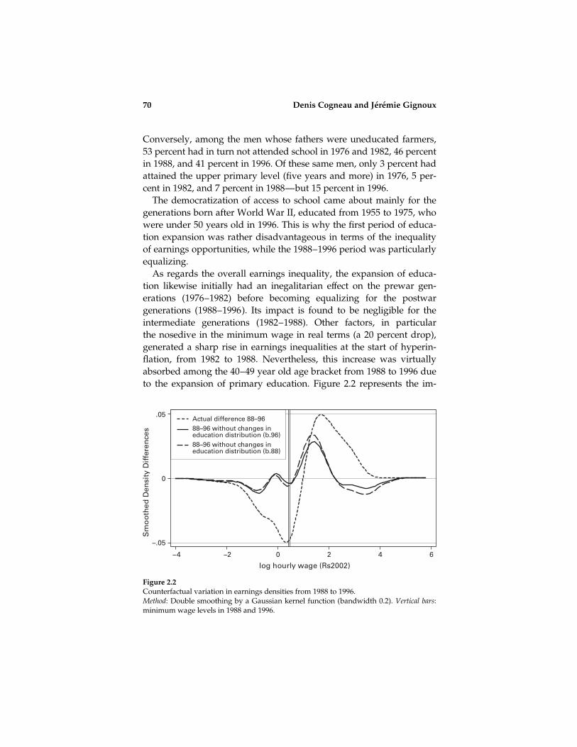
Figure 2.2
Counterfactual variation in earnings densities from 1988 to 1996.Method: Double smoothing by a Gaussian kernel function (bandwidth 0.2). Vertical bars:minimum wage levels in 1988 and 1996.
70 Denis Cogneau and Jeremie Gignoux

pact of this expansion of primary schooling on the development of
earnings densities in the last period. Vertical bars indicate the mini-
mum wages levels in 1988 (right) and 1996 (left). It suggests that the
observed reduction in poverty and inequalities would have been much
lower without this change in the marginal distribution of education
levels. The only notable development would have been a concentration
of the distribution to the right of the minimum wage, probably due to
the slow recovery in growth in the early 1990s and the end of hyper-
inflation in 1995.
Secondly, the change in the structure of earnings by education level
and type of social origin had an egalitarian effect at the end of the pe-
riod, in particular in the form of a sharp drop in returns to education
from 1988 to 1996. For example, the ratio of hourly average earnings
for uneducated men whose father was also uneducated to those of
men with a secondary education whose father had reached the same
education level was 11.4 in 1976 and 10.5 in 1982, rising to 11.3 in 1988
following a fall of over 15 percent in uneducated men’s earnings,
but finally descending to 8.8 in 1996. Over the 1988–1996 period,
the narrowing of the earnings scale contributed almost equally with
the expansion of primary education to the reduction in inequality of
opportunity.
Lastly, table 2.11 shows that changes in intergenerational educa-
tional mobility for the generations born from 1927 to 1956 were too
small to play a significant part in the developments observed. As the
following section argues, this explains the persisting inequality of eco-
nomic opportunity at a high level.
2.6 The Potential Effects of an Increase in Education Mobility on
Earnings Inequalities
2.6.1 Methodology
It is also possible to consider counterfactual population structures
other than the distributions observed for another year t 0. We construct,
for each year, the educational mobility matrices corresponding to the
independence assumption
pðiÞt ðs; oÞ ¼ ptðs; :Þptð:; oÞ ð2:14Þ
where ptðs; :Þ (resp. ptð:; oÞÞ stand for the row (resp. column) frequency
of schooling level s (resp. origin o).
Earnings Inequality, Educational Mobility in Brazil over Two Decades 71

Table
2.11
Historicaldecomposition19
76–19
96
1976
–1982
1982
–1988
1988
–1996
M:Ed.
mobility
D:
Distribution
S:Earnings
M:Ed.
mobility
D:Distribution
S:Earnings
M:Ed.
mobility
D:Distribution
S:Earnings
Ineq
ualityof
opportunity
effect
s.error
effect
s.error
effect
s.erroreffect
s.error
effect
s.error
effect
s.erroreffect
s.error
effect
s.error
effect
s.error
MDS
�0.005
0.029
0.016
0.012
�0.003
0.020
�0.002
0.004
0.011
0.006
0.011
0.011
�0.003
0.006
�0.041
0.005
�0.023
0.012
DMS
�0.001
0.011
0.013
0.019
�0.003
0.020
0.000
0.005
0.008
0.006
0.011
0.011
�0.003
0.006
�0.041
0.005
�0.023
0.012
SMD
0.011
0.014
0.024
0.013
�0.027
0.047
�0.004
0.005
0.012
0.007
0.012
0.010
�0.001
0.006
�0.035
0.005
�0.031
0.013
SDM
0.011
0.012
0.024
0.015
�0.027
0.047
�0.001
0.005
0.009
0.007
0.012
0.010
0.000
0.006
�0.036
0.005
�0.031
0.013
Var.
s.error
Var.
s.error
Var.
s.error
Total
variation
0.008
0.026
0.020
0.016
�0.067
0.016
percentages
over
the
total:
MDS
�60%
201%
�41%
�12%
56%
57%
5%61%
34%
DMS
�17%
158%
�41%
2%41%
57%
4%62%
34%
SMD
141%
301%
�341%
�19%
59%
60%
2%53%
46%
SDM
139%
302%
�341%
�4%
44%
60%
0%54%
46%
72 Denis Cogneau and Jeremie Gignoux

M:Ed.
mobility
D:
Distribution
R:Residual
M:Ed.
mobility
D:Distribution
R:Residual
M:Ed.
mobility
D:Distribution
R:Residual
Overall
ineq
uality
effect
s.error
effect
s.error
effect
s.erroreffect
s.error
effect
s.error
effect
s.erroreffect
s.error
effect
s.error
effect
s.error
MDR
�0.014
0.016
0.019
0.016
0.058
0.031
0.001
0.003
0.000
0.007
0.082
0.025
0.002
0.004
�0.052
0.006
0.001
0.035
DMR
�0.019
0.013
0.024
0.013
0.058
0.031
0.002
0.003
0.000
0.007
0.082
0.025
0.002
0.003
�0.052
0.006
0.001
0.035
SMR
�0.006
0.021
0.025
0.017
0.044
0.035
0.001
0.003
�0.001
0.006
0.084
0.026
�0.001
0.005
�0.039
0.010
�0.010
0.031
RDM
�0.004
0.011
0.022
0.012
0.044
0.035
0.002
0.003
�0.002
0.007
0.084
0.026
�0.001
0.004
�0.038
0.011
�0.010
0.031
Var.
s.error
Var.
s.error
Var.
s.error
Total
variation
0.063
0.035
0.084
0.025
�0.049
0.035
percentages
over
the
total:
MDR
�22%
30%
93%
2%0%
98%
�4%
106%
�3%
DMR
�30%
38%
93%
2%0%
98%
�3%
106%
�3%
RMD
�10%
40%
70%
1%�1%
100%
2%79%
20%
RDM
�6%
36%
70%
2%�2%
100%
2%78%
20%
Reading:
Sem
iparam
etricdecompositionofvariationsin
theVan
deGaerineq
ualityofopportunityindices
andoverallineq
ualityindices
interm
sof
theresp
ectiveeffectsofch
anges
ined
ucational
mobility,marginal
distributionsoforiginsan
ded
ucationlevels,an
dearningsfrom
1976
to19
96.T
he
simulationpathsarenotedbytheorder
ofch
anges,withM
den
otinged
ucational
mobility,D
themarginal
distributionsofsocial
originsan
ded
uca-
tionlevels,an
dSthestructuresofearningsbyed
ucationlevel
andtypeoforigin
orRtheresidual
(see
text).Standarddev
iations(s.e.)obtained
by
bootstrap
pingwith50
replications.
Earnings Inequality, Educational Mobility in Brazil over Two Decades 73

We then apply these perfect mobility matrices to the earnings struc-
tures observed in the year t considered, and hence estimate the total
contribution of educational mobility to the observed inequalities. This
type of counterfactual simulation leaves the population distributions
by type of origin and especially by education level invariant. It could
therefore be thought that the general equilibrium effects count less,
since the educational supply remains similar. However, there is an ex-
tensive redistribution of the population within the educational mobil-
ity matrix. So the assumption of the absence of selection effects and
especially the exogeneity of social origin as regards the unobserved
earning determinants has a large weight here. Our theoretical scenario
consists of simulating a fictitious world far removed from reality in
which the children of university-educated fathers stand as much
chance of failing at primary school as the children of illiterate fathers.
To illustrate this simulation, we again assume that there are only
two groups of social origins and two groups of education and that the
distribution observed on date t is given by frequency table 2.12. Two
individuals of different origin then are sixteen times more likely to
reproduce their fathers’ situations than to change them (reproduction
coefficient of 16). Perfect educational mobility can be simulated by
seeking the population structure that retains the marginal distributions
(0.50; 0.50) of education levels and origins, but such that two individu-
als of different origins stand as much chance of changing their situa-
tions as of reproducing them (odds ratio of 1). Table 2.13 presents the
frequencies for such a simulated distribution. The probabilities of
reaching a given level of education conditional on origins are equal.
The counterfactual earnings densities are obtained by reweighting
the observations by the ratios of values between tables 2.12 and 2.13,
based on the formula given by equation (2.6). The counterfactual in-
Table 2.12
Frequencies of the assumed distribution observed in t and average earnings by level ofeducation and type of origin
Education 1 Education 2
Origins 1 0.40y11
0.10y12
Origins 2 0.10y21
0.40y22
Note: Marginal distributions (0.50; 0.50) and odds-ratio of 16.
74 Denis Cogneau and Jeremie Gignoux
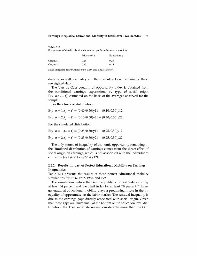
dices of overall inequality are then calculated on the basis of these
reweighted data.
The Van de Gaer equality of opportunity index is obtained from
the conditional earnings expectations by type of social origin
Eðy j o; ty ¼ tÞ, estimated on the basis of the averages observed for the
sample.
For the observed distribution:
Eðy j o ¼ 1; ty ¼ tÞ ¼ ð0:40=0:50Þy11þ ð0:10=0:50Þy12
Eðy j o ¼ 2; ty ¼ tÞ ¼ ð0:10=0:50Þy21þ ð0:40=0:50Þy22
For the simulated distribution:
Eðy j o ¼ 1; ty ¼ tÞ ¼ ð0:25=0:50Þy11þ ð0:25=0:50Þy12
Eðy j o ¼ 2; ty ¼ tÞ ¼ ð0:25=0:50Þy21þ ð0:25=0:50Þy22
The only source of inequality of economic opportunity remaining in
the simulated distribution of earnings comes from the direct effect of
social origin on earnings, which is not associated with the individual’s
education (y210 y11 et y220 y12).
2.6.2 Results: Impact of Perfect Educational Mobility on Earnings
Inequalities
Table 2.14 presents the results of these perfect educational mobility
simulations for 1976, 1982, 1988, and 1996.
The simulations reduce the Gini inequality of opportunity index by
at least 54 percent and the Theil index by at least 78 percent.18 Inter-
generational educational mobility plays a predominant role in the in-
equality of opportunity on the labor market. The residual inequality is
due to the earnings gaps directly associated with social origin. Given
that these gaps are fairly small at the bottom of the education level dis-
tribution, the Theil index decreases considerably more than the Gini
Table 2.13
Frequencies of the distribution simulating perfect educational mobility
Education 1 Education 2
Origins 1 0.25 0.25
Origins 2 0.25 0.25
Note: Marginal distributions (0.50; 0.50) and odds-ratio of 1.
Earnings Inequality, Educational Mobility in Brazil over Two Decades 75

index. Nevertheless, this difference in variation between the two indices
depends to a large extent on the sound estimation of the social origin
effects in cells with low or zero values in the educational mobility
matrices.
As regards overall inequality, figure 2.3, estimated by double kernel
smoothing, shows that perfect educational mobility not surprisingly
concentrates the distribution of earnings around the average. How-
ever, under our assumptions, the equalization of educational opportu-
nities only generates a reduction of one to three Gini index points
depending on the year, or a relative reduction of two to five percent
(table 2.14). Here again, the variation in the Theil index is greater, be-
tween 4 and 13 percent (10 percent in 1996) for the aforementioned
reason. For 1996, this last finding is in line with the seven percent
obtained by Bourguignon, Ferreira, and Menendez (2007) for the same
age bracket as regards the indirect (education-related) effect of social
origin on earnings inequality.
Table 2.14
Simulations of perfect educational mobility
1976 1982 1988 1996
Inequality ofopportunity
Gini indexSimulated variation �0.184 0.015 �0.260 0.009 �0.266 0.017 �0.186 0.008Observed 0.341 0.026 0.351 0.008 0.366 0.007 0.315 0.008
�54% �74% �73% �59%
Theil indexSimulated variation �0.163 0.016 �0.207 0.009 �0.220 0.014 �0.142 0.008Observed 0.209 0.030 0.222 0.009 0.242 0.010 0.171 0.009
�78% �93% �91% �83%
Overall inequality
Gini indexSimulated variation �0.009 0.017 �0.028 0.006 �0.032 0.009 �0.026 0.010Observed 0.570 0.009 0.586 0.005 0.623 0.004 0.597 0.005
�2% �5% �5% �4%
Theil indexSimulated variation �0.028 0.055 �0.074 0.019 �0.100 0.030 �0.069 0.043Observed 0.626 0.030 0.687 0.021 0.771 0.017 0.712 0.024
�4% �11% �13% �10%
Reading: Comparison of Van de Gaer inequality of opportunity indices and overallinequality indices observed and obtained by simulating independence between educa-tion levels and social origins. Standard deviations obtained by bootstrapping with 50replications.
76 Denis Cogneau and Jeremie Gignoux

However, both of our decompositions attribute a larger weight to
the indirect channel going through educational mobility. When look-
ing at the same cohorts (born between 1947 and 1956) in the same year
(1996), and for overall inequality decomposition, we obtain a 42/58
indirect/direct sharing against 18/82 in Bourguignon, Ferreira, and
Menendez (2007). Three main differences might explain this diver-
gence between the two studies. A first one lies in the decomposition
methology: nonparametric versus parametric. The second lies in the
list of origin variables: rather restricted in our case (nine categories)
due to the sample size constraints that bear on semiprametric estima-
tions, but rather long in their case (with race, region of birth, and
father’s detailed occupation included, even if parental education ends
up as the most important variable). A third and maybe more important
difference lies in the sample selection, national versus urban, even
though Bourguignon, Ferreira, and Menendez try to account for migra-
tion bias. Further research is warranted in order to understand the
source of this divergence.
Coming back to the weight of educational mobility in overall
inequality, we agree with Bourguignon, Ferreira, and Menendez in
Figure 2.3
Differences between observed densities and simulated densities with perfect educationalmobility.Method: Densities simulated by reweighting using the formula given by equation (2.6)and based on educational mobility matrices, where origin and education level are inde-pendent, estimated using the formula given in equation (2.14).
Earnings Inequality, Educational Mobility in Brazil over Two Decades 77

saying that our estimates as well as theirs only represent a lower
bound. Contrary to the simulations regarding the inequality of oppor-
tunity indices, but also contrary to the historical decompositions
presented in section 2.5, this last decomposition is indeed highly sensi-
tive to measurement errors and transient components in the analyzed
variable—here, hourly earnings. This is intuitively understood since
this static decomposition can only concern the proportion of inequality
corresponding to actual and permanent earnings gaps. In the working
paper version of this chapter (Cogneau and Gignoux 2005), we use a
simple case (log-normality) to show the effect of measurement errors
or irrelevant transitory components in terms of their share in the vari-
ance of the analyzed variable. The review of the literature by Bound,
Brown, and Mathiowetz (2001) suggests that a proportion of 20 to 30
percent is not unreasonable in the case of the measurement of hourly
earnings. Yet the simulations show that a proportion of 20 percent can
reduce the true effect threefold, while a proportion of 30 percent re-
duces it four- or fivefold. These approximations obviously only serve
as notional examples, since they are based on particularly simple
assumptions: the log-normality of the variables and multiplicative
white noise errors. Moreover, other contradictory arguments could at-
tenuate this underestimation of the effect of social origins on earnings
(endogeneity).
In the case of the inequality of opportunity indices, the practice of
considering averages or quantiles by type of social origin at least par-
tially offsets these measurement errors. However, such a discussion
calls for caution with regard to this theoretical scenario of perfect edu-
cational mobility, which has no close or even remote basis in historical
fact, since intergenerational educational mobility varies little over the
twenty years analyzed.19
2.7 Conclusion
This paper studies the impact of changes in educational opportunity
on overall inequality and the inequality of opportunity on the labor
market in Brazil over two decades. We use four editions of the na-
tionally representative PNAD survey to analyze growth in earnings
inequalities among 40–49-year-old men. We design and implement
semiparametric decompositions of the respective effects of schooling
expansion, changes in the structure of earnings, and changes in inter-
generational educational mobility.
78 Denis Cogneau and Jeremie Gignoux
Earnings inequalities varied little over the period, with a peak in the
late 1980s probably largely due to hyperinflation, which raged through
to 1994 (a four-figure rate). First of all, the decompositions show that
changes in the distribution of education contributed to the increase in
both types of inequality among the oldest generations before sharply
reducing them among the post-WWII cohorts. Second, the decrease
in returns to education also contributed to equalizing labor market
opportunities in the 1988–1996 period. Lastly, the changes in educa-
tional mobility were not large enough to significantly affect earnings
inequalities, whereas it is shown that they should play a prominent
role in equalizing opportunities in the future.
Brazil’s history, at least during the macroeconomic crisis and adjust-
ment period analyzed here, is one of steadily high income inequality.
This rigidity of inequality is observed despite the expansion of educa-
tion and despite the drop in returns to education, as already observed
by Lam in 1991 and by Ferreira and de Barros for household income
(2000 and 2004). Among the generations born before World War II,
growth in education mainly concerned the spread of access to second-
ary and higher education for the children of the upper classes, which
increased the inequality, as already noticed by Fishlow (1972). It was
only with the postwar generations that the expansion of primary edu-
cation and the opening of the secondary system to children of farmers
and of fathers with very little education started to play a major role in
the reduction of earnings inequalities. The decrease in returns to edu-
cation underpinned this reduction during the period of slow growth
recovery from 1988 to 1996 (marked by the Cardoso presidency and
the real plan).
This last period of education-related reduction in earnings inequality
could give rise to optimism as to the long-run effects of programs to
educate poor children, such as conditional cash-transfer programs. The
period also saw a slight upturn in intergenerational educational mobil-
ity, but this increase was too small to play a significant role in reducing
the inequality of opportunity and overall inequality. The expansion of
education prompted a race for qualifications and a quality race, both
of which probably contributed to the decrease in returns to years of
education. It will probably not be possible to attain a greater reduction
in inequality via education in the future without a marked increase in
intergenerational educational mobility. Yet it is still too soon to know
whether targeted educational programs will manage to significantly
stimulate this mobility.20
Earnings Inequality, Educational Mobility in Brazil over Two Decades 79
Acknowledgements
The authors would like to thank Francisco Ferreira, Michael Grimm,
Marc Gurgand, Stephan Klasen, Sylvie Lambert, and Petra Todd, as
well as two anonymous referees, and participants at an Education Day
at INED in Paris, at the AFSE development economics meeting at
CERDI in Clermont-Ferrand, at the Ibero-America Conference in Got-
tingen, and at the first ECINEQ conference in Palma de Mallorca. The
views expressed in this paper are those of the authors alone.
Notes
1. Only the rural areas of Tocantins State were covered in this region.
2. For 1976, this information was collected solely for a subsample representing approxi-mately 25 percent of the total sample.
3. In 1976, the question concerned the father’s education when the individual was 15years old.
4. This information was not collected by the 1982 PNAD.
5. The information on earned income is collected by a single question covering bothwage and nonwage activities.
6. We thank Pierre-Emmanuel Couralet for his help in building the databases.
7. Since the 1990s, the first two levels of the Brazilian education system have been theelementary level (equivalent to primary education), lasting for eight years and normallycovering children aged 7 to 14, and the intermediate level (equivalent to secondary edu-cation), lasting for three years and normally covering children aged 15 to 17. However,when the cohorts studied in this paper were educated, a basic level also existed coveringthe first four years of the elementary level.
8. We computed the hourly earnings means for 26 birth regions and grouped regionsinto four categories according to earnings differentials and geographical homogeneity.We also tried to preserve a balance in sample sizes. The highest levels of wages areobserved in category 1 and the lowest in category 2.
9. A second stratification at the level of the municipalities of the metropolitan strata, themain municipalities, and grouping of municipalities of the other strata cannot be takeninto account since the data do not enable these strata to be identified.
10. In the case when the number of types to be considered is too large, we implementthis type of measurement by estimating decile regressions of earnings (Koenker and Bas-sett 1978), using dummy variables for the different types of social origin. This means weassume that the effects of the origin variables are additive. This assumption enables us toestimate a decile level for a large number of types (128) when considering the four socialorigin variables (see section 2.2). In this latter case, direct nonparametric estimates are ineffect impossible due to sample size limitations.
80 Denis Cogneau and Jeremie Gignoux
11. Here again we use an intermediate regression step when considering 128 types of or-igin. We estimate an OLS earnings regression with the dummy variables for social originsas explanatory variables. The predictions resulting from this regression are the averageearnings conditional on the different categories of origin. When the nine-category originvariable is used so that sample sizes are large enough, we estimate the means directly ina nonparametric way.
12. These minimum earnings are not normed by the average. The growth presentedtherefore includes an absolute component (growth in welfare) and a relative component(Rawlsian inequality index). The growth in average earnings is nevertheless virtuallyzero throughout the entire period.
13. Earnings inequality is slightly underestimated by the exclusion of unemployed andinactive men from the sample. This bias increases with unemployment and inactivity in1996, but the decrease in inequality remains significant: the Theil index in 1988 reaches0.83 when including null wages against 0.77 with strictly positive wages; in 1996 theTheil index is 0.80 against 0.70. Regarding inequality of opportunity, the sample selectionseems completely innocuous. The Van de Gaer Theil index, with nine groups of socialorigins, is underestimated by 0.001—that is, by less than 1 percent. This very small re-duction mainly comes from the higher employment rates of men whose fathers wereworking in agriculture.
14. For 2� 2 transition matrices, there is a strict equality between the unique g coefficientand the unique odd-ratio. For transition matrices of a higher dimension (like 9� 9 here),equation (2.3) implies
Ln½Odd-Rtðs; o; s 0; o 0Þ� ¼ ½gðs; oÞ þ gtðs; oÞ þ gðs; oÞ þ gtðs; oÞ�
� ½gðs 0; oÞ þ gtðs 0; oÞ þ gðs; o 0Þ þ gtðs; o 0Þ�:
15. Bourguignon, Ferreira, and Menendez (2003) address the question of the endogeneityof education levels by making simulations under a number of assumptions of correlationbetween education level and wage unobservables. The origin variables are neverthelessassumed to be exogenous, an assumption that is also open to debate.
16. In contrast with section 2.4, we do not stack the contingency tables of different years;log-linear models are then written and estimated independently for each year.
17. The decomposition of the Gini indices can be found in the working paper version ofthis chapter (Cogneau and Gignoux 2005). They do not differ much from the decomposi-tions based on the Theil index.
18. These reductions are found to be smaller in certain cases due to the existence of sev-eral empty cells, reducing the education level value taken into account in the constructionof the notional matrices of perfect mobility, and hence the extent of the redistribution be-tween education levels.
19. In the case of the historical decompositions of section 2.4, the main factor likely toconfound the estimates is a variation in the variance proportion of these errors, due to achange in survey quality or methodology. Yet the effect of constant measurement errorsis largely eradicated by the consideration of time differences. In addition, all of thesedecompositions remain influenced by the measurement errors associated with the analy-sis variables (level of education and social origin) and by the selection and endogeneitybiases affecting the causal effect of these variables on earnings.
Earnings Inequality, Educational Mobility in Brazil over Two Decades 81

20. A recent paper from Ferreira, Leite, and Litchfield (2006) reveals a significant fall inhousehold income inequality between 1993 and 2004, which they associate with five fac-tors: declining inflation, sharp declines in the returns to education, pronounced rural-urban convergence, increases in the social transfers targeted to the poor, and a possibledecline in racial inequality.
References
Andrade, E., S. Ferreira, R. Madalozzo, and F. Veloso. 2003. ‘‘Do Borrowing ConstraintsDecrease Intergenerational Mobility in Brazil? A Test Using Quantile Regression.’’ Work-ing Paper, IBMEC.
Arias, O., G. Yamada, and L. Tejerina. 2002. ‘‘Education, Family Background and RacialEarnings Inequality in Brazil.’’ Working Paper, Inter-American Development Bank,Washington, D.C.
Bertail, P., and P. Combris. 1997. ‘‘Bootstrap Generalise d’un Sondage.’’ Annales d’Econo-mie et de Statistiques 46: 49–83.
Bishop, Y., S. Fienberg, and P. Holland. 1975. Discrete Multivariate Analysis: Theory and
Practice. Cambridge, MA: MIT Press.
Blinder, A. S. 1973. ‘‘Wage Discrimination: Reduced Form and Structural Estimates.’’Journal of Human Resources 8, no. 4: 436–455.
Bound, J., C. Brown, and N. Mathiowetz. 2001. ‘‘Chapter 59: Measurement Error in Sur-vey Data.’’ In Handbook of Econometrics, vol. 5, eds. J. J. Heckman and E. Leamer, 3705–3843. Amsterdam: North-Holland.
Bourguignon, F., F. H. G. Ferreira, and P. G. Leite. 2003. ‘‘Conditional Cash Transfers,Schooling, and Child Labor: Micro-Simulating Brazil’s Bolsa Escola Program.’’ World
Bank Economic Review 17, no. 2: 229–254.
Bourguignon, F., F. H. G. Ferreira, and M. Menendez. 2007. ‘‘Inequality of Opportunity inBrazil’’, Review of Income and Wealth 53, no. 4: 585–618.
Cogneau, D., and J. Gignoux. 2005. ‘‘Earnings Inequalities and Educational Mobilityin Brazil over Two Decades.’’ Working Paper 2005/03, DIAL, Paris, and DiscussionPaper No. 121, Ibero-America Institute for Economic Research, University of Gottingen.Available at http://www.dial.prd.fr/dial_publications/PDF/Doc_travail/2005–03.pdfor http://wiwi.uni-goettingen.de/vwlseminar/working_papers/ibero/DB121.pdf.
Di Nardo, J., N. Fortin, and T. Lemieux. 1996. ‘‘Labor Market Institutions and the Distri-bution of Wages, 1973–1992: A Semiparametric Approach.’’ Econometrica 64, no. 5: 1001–1044.
Dunn, C. E. 2007. ‘‘The Intergenerational Transmission of Lifetime Earnings: Evidencefrom Brazil’’, The B.E. Journal of Economic Analysis & Policy 7, no. 2 (Contributions), Arti-cle 2.
Ferreira, F. H. G., P. Lanjouw, and M. Neri. 2003. ‘‘A Robust Poverty Profile for BrazilUsing Multiple Data Sources.’’ Revista Brasileira de Economia 57, no. 1: 60–92.
Ferreira, F. H. G., and R. Paes de Barros. 2000. ‘‘Education and Income Distribution inUrban Brazil, 1976–1996.’’ CEPAL Review 71: 41–61.
82 Denis Cogneau and Jeremie Gignoux

Ferreira, F. H. G., and R. Paes de Barros. 2004. ‘‘The Slippery Slope: Explaining the In-crease in Extreme Poverty in Urban Brazil, 1976–96.’’ In The Microeconomics of Income Dis-
tribution Dynamics in East Asia and Latin America, eds. F. Bourguignon, F. H. G. Ferreira,and N. Lustig, 83–124. Washington, D.C. and New York: World Bank and Oxford Uni-versity Press.
Ferreira, F. H. G., P. G. Leite, and J. A. Litchfield. 2006. ‘‘The Rise and Fall of Brazilian In-equality: 1981–2004.’’ Policy Research Working Paper 3867, World Bank, Washington,D.C.
Ferreira, S., and F. Veloso. 2006. ‘‘Intergenerational Mobility of Wages in Brazil.’’ BrazilianReview of Econometrics 26, no. 2: 181–211.
Fishlow, A. 1972. ‘‘Brazilian Size Distribution of Income.’’ American Economic Review 62,no. 1–2: 391–402.
Juhn, C., K. M. Murphy, and B. Pierce. 1993. ‘‘Wage Inequality and the Rise in Returns toSkill.’’ Journal of Political Economy 101, no. 3: 410–442.
Koenker, R., and G. Bassett. 1978. ‘‘Regression Quantiles.’’ Econometrica 46, no. 1: 33–50.
Lam, D. 1999. ‘‘Generating Extreme Inequality: Schooling, Earnings, and Intergenera-tional Transmission of Human Capital in South Africa and Brazil.’’ Research Report, Pop-ulation Studies Center, University of Michigan.
Lam, D., and D. Levison. 1991. ‘‘Declining Inequality in Schooling in Brazil and its Effectson Inequality in Earnings.’’ Journal of Development Economics 37, no. 1/2: 199–225.
Lam, D., and R. Schoeni. 1993. ‘‘Effects of Family Background on Earnings and Returns toSchooling: Evidence from Brazil.’’ Journal of Political Economy 101, no. 4: 710–740.
Leite, P. G. 2006. ‘‘L’efficacite de Bolsa Escola par la Methode RDD.’’ Mimeo, EHESS andDIAL.
Lemieux, T. 2002. ‘‘Decomposing Changes in Wage Distributions: A Unified Approach.’’Canadian Journal of Economics 35, no. 4: 646–688.
Manski, C., and J. Pepper. 2000. ‘‘Monotone Instrumental Variables: With an Applicationto the Returns to Schooling.’’ Econometrica 68, no. 4: 997–1010.
Oaxaca, R. 1973. ‘‘Male-Female Wage Differentials in Urban Labor Markets.’’ InternationalEconomic Review 14, no. 3: 673–709.
Pastore, J. 1982. Inequality and Social Mobility in Brazil. Chicago: University of WisconsinPress.
Pastore, J., and N. Valle Silva. 2000. ‘‘Mobilidade Social no Brasil.’’ Sao Paulo: MakronBooks.
Pesquisa National por Amostra de Domicılios (PNAD) 1976–1996. ‘‘Notas methodologi-cas’’, Instituto Brasileiro de Geografia e Estatıstica, Rio de Janeiro. For more information:http://www.ibge.gov.br/home/estatistica/populacao/trabalhoerendimento/pnad2006/default.shtm
Picanco, F. 2004. ‘‘Economic Modernization and Socio-Occupational Mobility in Brazil.’’Communication presented at the International Sociological Association, RC28.
Roemer, J. 1996. Theories of Distributive Justice. Cambridge, MA: Harvard UniversityPress.
Earnings Inequality, Educational Mobility in Brazil over Two Decades 83

Roemer, J. 1998. Equality of Opportunity. Cambridge, MA: Harvard University Press.
Shorrocks, A. 1978. ‘‘The Measurement of Mobility.’’ Econometrica 46, no. 5: 1013–1024.
Sokoloff, K., and S. Engerman. 2000. ‘‘History Lessons: Institutions, Factor Endowments,and Paths of Development in the New World.’’ Journal of Economic Perspectives 14, no. 3:217–232.
Van de Gaer, D. 1993. ‘‘Equality of opportunity and investment in human capital’’, Catho-lic University of Leuven, Faculty of Economics, no. 92.
Van de Gaer, D., E. Schokkaert, and M. Martinez. 2001. ‘‘Three Meanings of Intergenera-tional Mobility.’’ Economica 68: 519–537.
84 Denis Cogneau and Jeremie Gignoux
Related Documents