NPTEL – Civil Engineering – Construction Economics & Finance Joint initiative of IITs and IISc – Funded by MHRD Page 1 of 107 Construction Economics & Finance Module 2 Lecture-1 Comparison of alternatives:- For most of the engineering projects, equipments etc., there are more than one feasible alternative. It is the duty of the project management team (comprising of engineers, designers, project managers etc.) of the client organization to select the best alternative that involves less cost and results more revenue. For this purpose, the economic comparison of the alternatives is made. The different cost elements and other parameters to be considered while making the economic comparison of the alternatives are initial cost, annual operating and maintenance cost, annual income or receipts, expected salvage value, income tax benefit and the useful life. When only one, among the feasible alternatives is selected, the alternatives are said to be mutually exclusive. As already mentioned in module-1, the cost or expenses are generally known as cash outflows whereas revenue or incomes are generally considered as cash inflows. Thus in the economic comparison of alternatives, cost or expenses are considered as negative cash flows. On the other hand the income or revenues are considered as positive cash flows. From the view point of expenditure incurred and revenue generated, some projects involve initial capital investment i.e. cash outflow at the beginning and show increased income or revenue i.e. cash inflow in the subsequent years. The alternatives having this type of cash flow are known as investment alternatives. So while comparing the mutually exclusive investment alternatives, the alternative showing maximum positive cash flow is generally selected. In this case, the investment is made at the beginning to gain profit at the future period of time. Example for such type alternatives includes purchase of a dozer by a construction firm. The construction firm will have different feasible alternatives for the dozer with each alternative having its own initial investment, annual operating and maintenance cost, annual income depending upon the production capacity, useful life, salvage values etc. Thus the alternative which will yield more economic benefit will be

Welcome message from author
This document is posted to help you gain knowledge. Please leave a comment to let me know what you think about it! Share it to your friends and learn new things together.
Transcript

8/15/2019 2 Comparision of Alternatives
http://slidepdf.com/reader/full/2-comparision-of-alternatives 1/107
NPTEL – Civil Engineering – Construction Economics & Finance
Joint initiative of IITs and IISc – Funded by MHRD Page 1 of 107
Construction Economics & Finance
Module 2
Lecture-1
Comparison of alternatives:-
For most of the engineering projects, equipments etc., there are more than one feasible
alternative. It is the duty of the project management team (comprising of engineers,
designers, project managers etc.) of the client organization to select the best alternative
that involves less cost and results more revenue. For this purpose, the economic
comparison of the alternatives is made. The different cost elements and other parameters
to be considered while making the economic comparison of the alternatives are initial
cost, annual operating and maintenance cost, annual income or receipts, expected salvage
value, income tax benefit and the useful life. When only one, among the feasible
alternatives is selected, the alternatives are said to be mutually exclusive.
As already mentioned in module-1, the cost or expenses are generally known as cash
outflows whereas revenue or incomes are generally considered as cash inflows. Thus in
the economic comparison of alternatives, cost or expenses are considered as negative
cash flows. On the other hand the income or revenues are considered as positive cash
flows. From the view point of expenditure incurred and revenue generated, some projects
involve initial capital investment i.e. cash outflow at the beginning and show increased
income or revenue i.e. cash inflow in the subsequent years. The alternatives having this
type of cash flow are known as investment alternatives. So while comparing the mutually
exclusive investment alternatives, the alternative showing maximum positive cash flow is
generally selected. In this case, the investment is made at the beginning to gain profit atthe future period of time. Example for such type alternatives includes purchase of a dozer
by a construction firm. The construction firm will have different feasible alternatives for
the dozer with each alternative having its own initial investment, annual operating and
maintenance cost, annual income depending upon the production capacity, useful life,
salvage values etc. Thus the alternative which will yield more economic benefit will be

8/15/2019 2 Comparision of Alternatives
http://slidepdf.com/reader/full/2-comparision-of-alternatives 2/107
NPTEL – Civil Engineering – Construction Economics & Finance
Joint initiative of IITs and IISc – Funded by MHRD Page 2 of 107
selected by the construction firm. There are some other projects which involve only costs
or expenses throughout the useful life except the salvage value if any, at the end of the
useful life. The alternatives having this type of cash flows are known as cost alternatives.
Thus while comparing mutually exclusive cost alternatives, the alternative showing
minimum negative cash flow is generally selected. Example for such type alternatives
includes construction of a government funded national highway stretch between two
regions. For this project there will be different feasible alternatives depending upon
length of the stretch, type of pavement, related environmental, social and regulatory
aspects etc. Each alternative will have its initial cost of construction, annual repair and
maintenance cost and some major repair cost if any, at some future point of time. The
alternative that will exhibit lowest cost will be selected for the construction of the
highway stretch.
The differences in different parameters namely initial capital investment, annual
operation cost, annually generated revenue, expected salvage value, useful life,
magnitude of output and its quality, performance and operational characteristics etc. may
exist among the mutually exclusive alternatives. Thus the economic analysis of the
mutually exclusive alternatives is generally carried out on the similar or equivalent basis
since each of the feasible alternatives will meet the desired requirements of the project, ifselected.
The economic comparison of mutually exclusive alternatives can be carried out by
different equivalent worth methods namely present worth method, future worth method
and annual worth method. In these methods all the cash flows i.e. cash outflows and cash
inflows are converted into equivalent present worth, future worth or annual worth
considering the time value of money at a given interest rate per interest period.

8/15/2019 2 Comparision of Alternatives
http://slidepdf.com/reader/full/2-comparision-of-alternatives 3/107
NPTEL – Civil Engineering – Construction Economics & Finance
Joint initiative of IITs and IISc – Funded by MHRD Page 3 of 107
Comparison of alternatives by present worth method:
In the present worth method for comparison of mutually exclusive alternatives, the future
amounts i.e. expenditures and incomes occurring at future periods of time are converted
into equivalent present worth values at a certain rate of interest per interest period and are
added to present worth occurring at „0 time. The converted equivalent present worth
values are always less than the respective future amounts since the rate of interest is
normally greater than zero. The cash flow of the mutually exclusive alternatives may
consist of future expenditures and incomes in different forms namely randomly placed
single amounts, uniform amount series commencing from end of year 1, randomly placed
uniform amount series i.e. commencing at time period other than end of year 1, positive
and negative uniform gradient series starting either from end of year 1 or at different time
periods and geometric gradient series etc. The different compound interest factors namely
single payment present worth factor, uniform series present worth factor and present
worth factors for arithmetic and geometric gradient series etc. will be used to convert the
respective future amounts to the equivalent present worth values for different alternatives.
The methodology for the comparison of mutually exclusive alternatives by the present
worth method depends upon the magnitude of useful lives of the alternatives. There are
two cases; a) the useful lives of alternatives are equal and b) the useful lives ofalternatives are not equal. The alternatives having equal useful lives are designated as
equal life span alternatives whereas the alternatives having unequal life spans are referred
as different life span alternatives.
a) Equal life span alternatives
The comparison of mutually exclusive alternatives having equal life spans by present
worth method is comparatively simpler than those having different life spans. In case of
equal life span mutually exclusive alternatives, the future amounts as already stated are
converted into the equivalent present worth values and are added to the present worth
occurring at time zero. Then the alternative that exhibits maximum positive equivalent
present worth or minimum negative equivalent present worth is selected from the
considered feasible alternatives.

8/15/2019 2 Comparision of Alternatives
http://slidepdf.com/reader/full/2-comparision-of-alternatives 4/107
NPTEL – Civil Engineering – Construction Economics & Finance
Joint initiative of IITs and IISc – Funded by MHRD Page 4 of 107
a) Different life span alternatives
In case of mutually exclusive alternatives, those have different life spans, the comparison
is generally made over the same number of years i.e. a common study period. This is
because; the comparison of the mutually exclusive alternatives over same period of time
is required for unbiased economic evaluation of the alternatives. If the comparison of the
alternatives is not made over the same life span, then the cost alternative having shorter
life span will result in lower equivalent present worth i.e. lower cost than the cost
alternative having longer life span. Because in this case, the cost of the short span
alternative is considered only for a shorter period of time, even though this alternative
may not be economical. In case of mutually exclusive investment alternatives, the
alternative with longer life span will result in higher equivalent present worth i.e. higher
positive equivalent worth, as the costs, revenues, savings through reduced costs is
considered over a longer period of time than the alternative with shorter life span. Thus in
order to minimize the effect of such kind of discrepancy on the selection of best
alternative from the considered feasible alternatives, the comparison is made over the
same life span.
The two approaches used for economic comparison of different life span alternatives are
as follows;i) Comparison of mutually exclusive alternatives over a time period that is equal to least
common multiple (LCM) of the individual life spans
ii) Comparison of mutually exclusive alternatives over a study period which is not
necessarily equal to the life span of any of the alternatives.
In the first approach the comparison is made over a time period equal to the least
common multiple of the life spans of mutually exclusive alternatives. The cash flow of
the alternatives i.e. cash flow of the first cycle is repeated and the number of repetitions
depends upon the value of least common multiple of life spans between the mutually
exclusive alternatives. It may be noted here that the cash flow i.e. all the costs and
revenues of the alternatives in the successive cycle will be exactly same as that in the first
cycle. For example if there are two alternatives with useful lives of 4 years and 5 years.

8/15/2019 2 Comparision of Alternatives
http://slidepdf.com/reader/full/2-comparision-of-alternatives 5/107
NPTEL – Civil Engineering – Construction Economics & Finance
Joint initiative of IITs and IISc – Funded by MHRD Page 5 of 107
Then the alternatives will compared over a period of 20 years (least common multiple of
life spans) at the given rate of interest per year. Thus the cash flow of the alternative
having the life span of 4 years will be repeated 5 times including the first cycle whereas
the cash flow of the alternative with life span of 5 years will be repeated 4 times
including the first cycle. After that the most economical alternative will be selected.
Taking another example, there are two alternatives with life spans of 5 years and 10
years. In this case the alternatives will be compared over a period of 10 years (LCM).
Thus the alternative with life span of 5 years will be analyzed for 2 cycles whereas the
alternative with 10 year life span will be analyzed for one cycle only at the given rate of
interest per year.
In the second approach, a study period is selected over which the economic comparison
of mutually exclusive alternatives is carried out. The length of the study period will
depend on the overall benefit of the project i.e. it may be shorter or longer (as compared
to useful lives of the individual alternatives) depending upon the short-term or long-term
benefits as desired for the project. Thus the cash flows of the alternatives occurring
during the study period are only considered for the economic comparison. However if
any alternative possesses salvage value at the end of its useful life and that occurs after
the study period, then its equivalent value must be included in the economic analysis. The
values of equivalent present worth of the mutually exclusive alternatives are calculatedover the selected study period and the alternative showing maximum positive equivalent
present worth or minimum negative equivalent present worth is selected.

8/15/2019 2 Comparision of Alternatives
http://slidepdf.com/reader/full/2-comparision-of-alternatives 6/107
NPTEL – Civil Engineering – Construction Economics & Finance
Joint initiative of IITs and IISc – Funded by MHRD Page 6 of 107
Lecture-2
Comparison by present worth method:-
Now some examples showing the use of present worth method for comparison of
mutually exclusive alternatives are presented. First the comparison of equal life span
mutually exclusive alternatives by present worth method will be illustrated followed by
comparison of different life span alternatives. The following examples are formulated
only to demonstrate the use of different methods for comparison of alternatives. The
values of different cost and incomes mentioned in the examples are not the actual ones
pertaining to a particular item. In addition it may also be noted here that the cash flow
diagrams have been drawn not to the scale. These are merely graphical representations.
Example -1
There are two alternatives for purchasing a concrete mixer. Both the alternatives have
same useful life. The cash flow details of alternatives are as follows;
Alternative-1: Initial purchase cost = Rs.3,00,000, Annual operating and maintenance
cost = Rs.20,000, Expected salvage value = Rs.1,25,000, Useful life = 5 years.
Alternative-2: Initial purchase cost = Rs.2,00,000, Annual operating and maintenance
cost = Rs.35,000, Expected salvage value = Rs.70,000, Useful life = 5 years.
Using present worth method, find out which alternative should be selected, if the rate of
interest is 10% per year.
Solution:
Since both alternatives have the same life span i.e. 5years, the present worth of the
alternatives will be compared over a period of 5 years. The cash flow diagram of
Alternative-1 is shown in Fig. 2.1.
As already mentioned Module-1, the cash outflows i.e. costs or expenditures are
represented by vertically downward arrows whereas the cash inflows i.e. revenue or
income are represented by vertically upward arrows. The same convention is adopted
here.

8/15/2019 2 Comparision of Alternatives
http://slidepdf.com/reader/full/2-comparision-of-alternatives 7/107
NPTEL – Civil Engineering – Construction Economics & Finance
Joint initiative of IITs and IISc – Funded by MHRD Page 7 of 107
Fig. 2.1 Cash flow diagram of Alternative-1
The equivalent present worth of Alternative-1 i.e. PW 1 is calculated as follows;
The initial cost, P = Rs.3,00,000 (cash outflow),
Annual operating and maintenance cost, A = Rs.20,000 (cash outflow),Salvage value, F = Rs.1,25,000 (cash inflow).
PW 1 = - 3,00,000 – 20,000( P/A, i, n ) + 1,25,000( P/F, i, n )
PW 1 = - 3,00,000 – 20,000( P/A, 10%, 5 ) + 1,25,000( P/F, 10%, 5 )
Now putting the mathematical expressions of different compound interest factors (as
mentioned in Module-1) in the above expression for PW 1 (in Rs.) results in the following;
nn
n
iii
i PW
1
1000,25,1
1
11000,20000,00,31
55
5
11.01
1000,25,1
1.011.0
11.01000,20000,00,3 PW
6209.0000,25,17908.3000,20000,00,31 PW
PW 1 = - 3,00,000 -75,816 + 77,613
PW 1 = - Rs.2,98,203
Rs.20,000
Rs.3,00,000
2 31 4 50
Rs.1,25,000
Time (Year)
Income
Expenditure

8/15/2019 2 Comparision of Alternatives
http://slidepdf.com/reader/full/2-comparision-of-alternatives 8/107
NPTEL – Civil Engineering – Construction Economics & Finance
Joint initiative of IITs and IISc – Funded by MHRD Page 8 of 107
The cash flow diagram of Alternative-2 is shown in Fig. 2.2.
Fig. 2.2 Cash flow diagram of Alternative-2
Now the equivalent present worth of Alternative-2 i.e. PW 2 (in Rs.) is calculated as
follows;The initial cost, P = Rs.2,00,000 (cash outflow),
Annual operating and maintenance cost, A = Rs.35,000 (cash outflow),
Salvage value, F = Rs.70,000 (cash inflow).
PW 2 = - 2,00,000 – 35,000( P/A, i, n ) + 70,000( P/F, i, n )
PW 2 = - 2,00,000 – 35,000( P/A, 10%, 5 ) + 70,000( P/F, 10%, 5 )
nn
n
iii
i PW
1
1000,70
1
11000,35000,00,22
55
5
21.01
1000,70
1.011.0
11.01000,35000,00,2 PW
6209.0000,707908.3000,35000,00,22 PW
PW 2 = - 2,00,000 – 1,32,678 + 43,463
PW 2 = - Rs.2,89,215
Comparing the equivalent present worth of both the alternatives, it is observed that
Alternative-2 will be selected as it shows lower negative equivalent present worth
compared to Alternative-1 at the interest rate of 10% per year.
The equivalent present worth of both the alternatives can also be calculated by using the
values of compound interest factors from interest tables. The equivalent present worth of
Alternative-1 i.e. PW 1 is calculated as follows;
PW 1 = - 3,00,000 – 20,000( P/A, i, n ) + 1,25,000( P/F, i, n )
Rs.2,00,000
2 31 4 50
Rs.35,000
Rs.70,000
Time (Year)

8/15/2019 2 Comparision of Alternatives
http://slidepdf.com/reader/full/2-comparision-of-alternatives 9/107

8/15/2019 2 Comparision of Alternatives
http://slidepdf.com/reader/full/2-comparision-of-alternatives 10/107
NPTEL – Civil Engineering – Construction Economics & Finance
Joint initiative of IITs and IISc – Funded by MHRD Page 10 of 107
Example -2
Alternative-1: Initial purchase cost = Rs.300000, Annual operating and maintenance cost
= Rs.20000, Expected salvage value = Rs.125000, Useful life = 5 years.
Alternative-2: Initial purchase cost = Rs.200000, Annual operating and maintenance cost
= Rs.35000, Expected salvage value = Rs.70000, Useful life = 5 years.
The annual revenue to be generated from production of concrete (by concrete mixer)
from Alternative-1 and Alternative-2 are Rs.50000 and Rs.45000 respectively. Compute
the equivalent present worth of the alternatives at the same rate of interest as in Example-
1 i.e. 10% per year and find out the economical alternative.
Solution:
The cash flow diagram of Alternative-1 is shown in Fig. 2.3.
Fig. 2.3 Cash flow diagram of Alternative-1
The equivalent present worth of Alternative-1 is calculated as follows;
PW 1 = - 300000 - 20000( P/A, i, n ) + 50000 (P/A, i, n) + 125000( P/F, i, n )
PW 1 = - 300000 - 20000( P/A, 10%, 5 ) + 50000( P/A, 10%, 5 ) + 125000( P/F, 10%, 5 )
PW 1 = - 300000 + (50000 – 20000) ( P/A, 10%, 5 ) + 125000( P/F, 10%, 5 )
PW 1 = - 300000 + 30000( P/A, 10%, 5 ) + 125000( P/F, 10%, 5 )
nn
n
iii
i PW
1
1125000
1
1130000300000
1
55
5
11.01
1125000
1.011.0
11.0130000300000 PW
6209.01250007908.3300003000001 PW
PW 1 = - 300000 + 113724 + 77613
300000
2 31 4 50
Rs.20000
Rs.125000
Time (Year)
Rs.50000

8/15/2019 2 Comparision of Alternatives
http://slidepdf.com/reader/full/2-comparision-of-alternatives 11/107
NPTEL – Civil Engineering – Construction Economics & Finance
Joint initiative of IITs and IISc – Funded by MHRD Page 11 of 107
PW 1 = - Rs.108663
The cash flow diagram of Alternative-2 is shown in Fig. 2.4.
Fig. 2.4 Cash flow diagram of Alternative-2
Now the equivalent present worth of Alternative-2 i.e. PW 2 (in Rs.) is calculated as
follows;
PW 2 = - 200000 - 35000( P/A, i, n ) + 45000 (P/A, i, n) + 70000( P/F, i, n )
PW 2 = - 200000 - 35000( P/A, 10%, 5 ) + 45000 (P/A, 10%, 5) + 70000( P/F, 10%, 5 )
PW 2 = - 200000 + (45000 – 35000) ( P / A, 10%, 5 ) + 70000( P/F, 10%, 5 )
PW 2 = - 200000 + 10000( P/A, 10%, 5 ) + 70000( P/F, 10%, 5 )
nn
n
iii
i PW 1
1700001
11100002000002
55
5
21.01
170000
1.011.0
11.0110000200000 PW
6209.0700007908.3100002000002 PW
PW 2 = - 200000 + 37908 + 43463
PW 2 = - Rs.118629
Comparing the equivalent present worth of the both the alternatives, it is observed that
Alternative-1 will be selected as it shows lower cost compared to Alternative-2. The
annual revenue to be generated by the alternatives made the difference as compared to the
outcome obtained in Example-1.
200000
2 31 4 50
Rs.35000
Rs.70000
Time (Year)
Rs.45000
8/15/2019 2 Comparision of Alternatives
http://slidepdf.com/reader/full/2-comparision-of-alternatives 12/107
NPTEL – Civil Engineering – Construction Economics & Finance
Joint initiative of IITs and IISc – Funded by MHRD Page 12 of 107
When there are more than two alternatives for the selection of the best economical
alternative by present worth method, the same procedure as mentioned earlier for the case
of two alternatives is followed and illustrated in the next example.
Example -3
A construction contractor has three options to purchase a dump truck for transportation
and dumping of soil at a construction site. All the alternatives have the same useful life.
The cash flow details of all the alternatives are provided as follows;
Option-1: Initial purchase price = Rs.2500000, Annual operating cost Rs.45000 at the
end of 1 st year and increasing by Rs.3000 in the subsequent years till the end of useful
life, Annual income = Rs.120000, Salvage value = Rs.550000, Useful life = 10 years.
Option-2: Initial purchase price = Rs.3000000, Annual operating cost = Rs.30000,
Annual income Rs.150000 for first three years and increasing by Rs.5000 in the
subsequent years till the end of useful life, Salvage value = Rs.800000, Useful life = 10
years.
Option-3: Initial purchase price = Rs.2700000, Annual operating cost Rs.35000 for first
5 years and increasing by Rs.2000 in the successive years till the end of useful life,
Annual income = Rs.140000, Expected salvage value = Rs.650000, Useful life = 10years.
Using present worth method, find out which alternative should be selected, if the rate of
interest is 8% per year.
Solution:
The cash flow diagram of Option-1 is shown in Fig. 2.5.

8/15/2019 2 Comparision of Alternatives
http://slidepdf.com/reader/full/2-comparision-of-alternatives 13/107
NPTEL – Civil Engineering – Construction Economics & Finance
Joint initiative of IITs and IISc – Funded by MHRD Page 13 of 107
Fig. 2.5 Cash flow diagram of Option-1
For Option-1, the annual operating cost is in the form of a positive uniform gradient
series with gradient starting from end of year „2 . T he operating cost at the end of
different years can be split into the uniform base amount of Rs.45000 and the gradient
amount in multiples of Rs.3000 as shown in Fig. 2.6.
Fig. 2.6 Cash flow diagram of Option-1
with annual operating cost split i nto uniform base amount and gradient amount
The present worth of the uniform gradient series will be located at the beginning i.e. in
year „0 i.e. 2 years before the commencement of the uniform gradient.
Time (Year)
Rs.72000
2 31 4 50
Rs.45000
Rs.550000
6 7 1098
Rs.120000
Rs.48000Rs.51000
Rs.54000Rs.57000
Rs.60000Rs.63000
Rs.66000
Rs.69000
Rs.2500000
2 31 4 50
Uniform amountRs.45000
Rs.550000
6 7 1098
Rs.120000
Rs.2500000Rs.3000
Rs.6000Rs.9000
Rs.12000Rs.15000
Rs.18000
Rs.21000
Rs.24000
Rs.27000
Time (Year)

8/15/2019 2 Comparision of Alternatives
http://slidepdf.com/reader/full/2-comparision-of-alternatives 14/107
NPTEL – Civil Engineering – Construction Economics & Finance
Joint initiative of IITs and IISc – Funded by MHRD Page 14 of 107
Now the equivalent present worth (in Rs.) of Option-1 is calculated as follows;
PW 1 = - 2500000 - 45000( P/A, i, n ) - 3000 (P/G, i, n) + 120000 (P/A, i, n) + 550000( P/F,
i, n )
PW 1 = - 2500000 - 45000 (P/A, 8%, 10) - 3000 (P/G, 8%, 10) + 120000 (P/A, 8%, 10) +
550000 (P/F, 8%, 10)
PW 1 = - 2500000 + (120000 - 45000) (P/A, 8%, 10) - 3000 (P/G, 8%, 10) + 550000 (P/F,
8%, 10)
Now putting the values of different compound interest factors (the expressions in terms
of ‘i’ and ‘n’ already stated in Module-1) in the above expression for PW 1 results in the
following;
4632.05500009768.2530007101.67500025000001 PW
PW 1 = - 2500000 + 503258 - 77930 + 254760
PW 1 = - Rs.1819912
The cash flow diagram of Option-2 is shown in Fig. 2.7.
Fig. 2.7 Cash flow diagram of Option-2
Time (Year)
Rs.180000
2 31 4 50
Rs.160000
Rs.800000
6 7 1098
Rs.150000
Rs.30000
Rs.185000
Rs.155000
Rs.165000
Rs.170000
Rs.175000
Rs.3000000

8/15/2019 2 Comparision of Alternatives
http://slidepdf.com/reader/full/2-comparision-of-alternatives 15/107
NPTEL – Civil Engineering – Construction Economics & Finance
Joint initiative of IITs and IISc – Funded by MHRD Page 15 of 107
For Option-2, the annual income is in the form of a positive uniform gradient series with
gradient starting from end of year „4 . The annual income can be split into the uniform
base amount of Rs.150000 and the gradient amount in multiples of Rs.5000 starting from
end of year „4 and is shown in Fig. 2.8.
Fig. 2.8 Cash flow diagram of Option-2 with
annual income split into uniform base amount and gradient amount
The equivalent present worth of the gradient series (of the annual income) starting from
end of year „4 will be located at the end of year „2 i.e. 2 years before the start of the
gradient. Further the present worth of this amount at beginning i.e. at time „0 will be
obtained by multiplying the equivalent present worth „ P g ’ (shown in Fig. 2.8) at the end
of year „2 (which is a future amount) with the single payment present worth factor (P/F,
i, n) .
Now the equivalent present worth (in Rs.) of Option-2 is determined as follows;
PW 2 = - 3000000 - 30000( P/A, 8%, 10 ) + 150000 (P/A, 8%, 10) + P g (P/F, 8%, 2) +
800000( P/F, 8%, 10 )
Now in the above expression, P g will be replaced by G (P/G, i, n) i.e. 5000( P/G, 8%, 8 ).
Time (Year)
Rs.35000
2 31 4 50
Rs.20000
6 7 1098
Uniform amountRs.150000
Rs.30000
Rs.15000
Rs.25000
Rs.10000
Rs.30000
Rs.3000000
Rs.5000Pg
Rs.800000

8/15/2019 2 Comparision of Alternatives
http://slidepdf.com/reader/full/2-comparision-of-alternatives 16/107
NPTEL – Civil Engineering – Construction Economics & Finance
Joint initiative of IITs and IISc – Funded by MHRD Page 16 of 107
PW 2 = - 3000000 - 30000( P/A, 8%, 10 ) + 150000 (P/A, 8%, 10) + 5000 (P/G, 8%, 8) (P/F,
8%, 2) + 800000( P/F, 8%, 10 )
PW 2 = - 3000000 + (150000 - 30000) (P/A, 8%, 10) + 5000 (P/G, 8%, 8) (P/F, 8%, 2) +
800000( P/F, 8%, 10 )
Now putting the values of different compound interest factors in the above expression for
PW 2 results in the following;
4632.08000008573.08061.1750007101.612000030000002 PW
PW 2 = - 3000000 + 805212 + 76326 + 370560
PW 2 = - Rs.1747902
The cash flow diagram of Option-3 is shown in Fig. 2.9.
Fig. 2.9 Cash flow diagram of Option-3
For Option-3, the annual operating cost is in the form of a positive uniform gradient
series with gradient starting fr om end of year „ 6 . The annual operating cost can thus be
split into the uniform base amount of Rs.35000 and the gradient amount in multiples of
Rs.2 000 starting from end of year „ 6 (shown in Fig. 2.10).
The equivalent present worth of the gradient series for the annual operating cost starting
from end of year „ 6 will be located at the end of year „ 4 . Further the present worth of
this amount at time „0 will be determined by multiplying the equivalent present worth
„ P g ’ (shown in Fig. 2.10) at the end o f year „ 4 with the single payment present worth
factor (P/F, i, n) .
Time (Year)
Rs.45000
2 31 4 50
Rs.35000
Rs.650000
6 7 1098
Rs.140000
Rs.37000Rs.39000
Rs.41000Rs.43000
Rs.2700000

8/15/2019 2 Comparision of Alternatives
http://slidepdf.com/reader/full/2-comparision-of-alternatives 17/107
NPTEL – Civil Engineering – Construction Economics & Finance
Joint initiative of IITs and IISc – Funded by MHRD Page 17 of 107
Fig. 2.10 Cash flow diagram of Option-3 with
annual operating cost split into uniform base amount and gradient amount
The equivalent present worth (in Rs.) of Option-3 is obtained as follows;
PW 3 = - 2700000 - 35000( P/A, 8%, 10 ) - P g (P/F, 8%, 4) + 140000 (P/A, 8%, 10) +
650000( P/F, 8%, 10 )
Now in the above expression, P g will be replaced by G (P/G, i, n) i.e. 2000( P/G, 8%, 6 ).
PW 3 = - 2700000 - 35000( P/A, 8%, 10 ) - 2000 (P/G, 8%, 6) (P/F, 8%, 4) + 140000 (P/A,
8%, 10) + 650000( P/F, 8%, 10 )
PW 3 = - 2700000 + (140000 - 35000) (P/A, 8%, 10) - 2000 (P/G, 8%, 6) (P/F, 8%, 4) +
650000( P/F, 8%, 10 )
Now putting the values of different compound interest factors in the above expression,
the value of PW 3 is given by;
4632.06500007350.05233.1020007101.610500027000003 PW
PW 3 = - 2700000 + 704561 - 15469 + 301080
PW 3 = - Rs.1709828
From the comparison of equivalent present worth of all the three mutually exclusivealternatives, it is observed that Option-3 shows lowest negative equivalent present worth
as compared to other options. Thus Option-3 will be selected for the purchase of the
dump truck.
Time (Year) 2 31 4 50
Uniform amountRs.35000
Rs.650000
6 7 1098
Rs.140000
Rs.2700000 Rs.2000Rs.4000
Rs.6000Rs.8000
Rs.10000
Pg

8/15/2019 2 Comparision of Alternatives
http://slidepdf.com/reader/full/2-comparision-of-alternatives 18/107
NPTEL – Civil Engineering – Construction Economics & Finance
Joint initiative of IITs and IISc – Funded by MHRD Page 18 of 107
Lecture-3
Comparison by present worth method:-
After the illustration of comparison of equal life span mutually exclusive alternatives,now some examples illustrating the use of present worth method for comparison of
different life span mutually exclusive alternatives are presented.
Example -4
A material testing laboratory has two alternatives for purchasing a compression testing
machine which will be used for determining the compressive strength of different
construction materials. The alternatives are from two different manufacturing companies.
The cash flow details of the alternatives are as follows;
Alternative-1: Initial purchase price = Rs.1000000, Annual operating cost = Rs.10000,
Expected annual income to be generated from testing of different construction materials =
Rs.175000, Expected salvage value = Rs.200000, Useful life = 10 years.
Alternative-2: Initial purchase price = Rs.700000, Annual operating cost = Rs.15000,
Expected annual income to be generated from testing of different construction materials =
Rs.165000, Expected salvage value = Rs.250000, Useful life = 5 years.
Using present worth method, find out the most economical alternative at the interest rateof 10% per year.
Solution:
The alternatives have different life spans i.e. 10 years and 5 years. Thus the comparison
will be made over a time period equal to the least common multiple of the life spans of
the alternatives. In this case the least common multiple of the life spans is 10 years. Thus
the cash flow of Alternative-1 will be analyzed for one cycle (duration of 10 years)
whereas the cash flow of Alternative-2 will be analyzed for two cycles (duration of 5
years for each cycle). The cash flow of the Alternative-2 for the second cycle will be
exactly same as that in the first cycle.

8/15/2019 2 Comparision of Alternatives
http://slidepdf.com/reader/full/2-comparision-of-alternatives 19/107
NPTEL – Civil Engineering – Construction Economics & Finance
Joint initiative of IITs and IISc – Funded by MHRD Page 19 of 107
The cash flow diagram of Alternative-1 is shown in Fig. 2.11.
Fig. 2.11 Cash flow diagram of Al ternative-1
The equivalent present worth PW 1 (in Rs.) of Alternative-1 is calculated as follows;
PW 1 = - 1000000 - 10000( P/A, i, n ) + 175000 (P/A, i, n) + 200000( P/F, i, n )
PW 1 = - 1000000 - 10000( P/A, 10%, 10 ) + 175000 (P/A, 10%, 10) + 200000( P/F, 10%,
10)
PW 1 = - 1000000 + (175000 - 10000) ( P/A, 10%, 10 ) + 200000( P/F, 10%, 10 )
Putting the values of different compound interest factors in the above expression for PW 1;
3855.02000001446.616500010000001 PW
PW 1 = - 1000000 + 1013859 + 77100
PW 1 = Rs.90959
The cash flow diagram of Alternative-2 is shown in Fig. 2.12. As the least commonmultiple of the life spans of the alternatives is 10 years, the cash flow of Alternative-2 is
shown for two cycles with each cycle of duration 5 years.
Time (Year)2 31 4 50
Rs.10000
Rs.200000
6 7 1098
Rs.175000
Rs.1000000

8/15/2019 2 Comparision of Alternatives
http://slidepdf.com/reader/full/2-comparision-of-alternatives 20/107
NPTEL – Civil Engineering – Construction Economics & Finance
Joint initiative of IITs and IISc – Funded by MHRD Page 20 of 107
Fig. 2.12 Cash flow diagram of Alternative-2 for two cycle s
In the cash flow diagram of Alternative-2, the initial purchase price of Rs.700000 is againlocated at the end of year „5 i.e. at the end of first cycle or the beginning of the second
cycle. In addition the annual operating cost and the annual income are also repeated in the
second cycle from end of year „6 till end of year „10 . Further the salvage value of
Rs.250000 is also located at end of year „10 i.e. at the end of second cyc le.
The equivalent present worth PW 2 (in Rs.) of Alternative-2 is determined as follows;
PW 2 = - 700000 - 15000( P/A, 10%, 10 ) + 165000 (P/A, 10%, 10) + 250000( P/F, 10%, 5 ) -
700000 (P/F, 10%, 5) + 250000 (P/F, 10%, 10) PW 2 = - 700000 + (165000 - 15000) ( P/A, 10%, 10 ) - (700000 – 250000) ( P/F, 10%, 5 ) +
250000 (P/F, 10%, 10)
Putting the values of different compound interest factors in the above expression for PW 2
results in the following;
3855.02500006209.04500001446.61500007000002 PW
PW 2 = - 700000 + 921690 - 279405 + 96375
PW 2 = Rs.38660
Thus from the comparison of equivalent present worth of the alternatives, it is evident
that Alternative-1 will be selected for purchase of the compression testing machine as it
shows the higher positive equivalent present worth.
Rs.250000
2 31 4 50
Rs.15000
6 7 1098
Rs.700000
Rs.250000
Rs.700000
Rs.165000
First Cycle Second Cycle
Time (Year)

8/15/2019 2 Comparision of Alternatives
http://slidepdf.com/reader/full/2-comparision-of-alternatives 21/107
NPTEL – Civil Engineering – Construction Economics & Finance
Joint initiative of IITs and IISc – Funded by MHRD Page 21 of 107
In the following example, the comparison of different life span mutually exclusive
alternatives having expenditure or income in the form of gradient series by present worth
method is illustrated.
Example -5
A construction firm has decided to purchase a dozer to be employed at a construction site.
Two different companies manufacture the dozer that will fulfill the functional
requirement of the construction firm. The construction firm will purchase the most
economical one from one of these companies. The alternatives have different useful lives.
The cash flow details of both alternatives are presented as follows;
Company-A Dozer: Initial purchase cost = Rs.3050000, Annual operating cost Rs.40000
at end of 1 st year and increasing by Rs.2000 in the subsequent years till the end of useful
life, Annual income = Rs.560000, Expected salvage value = Rs.1050000, Useful life = 6
years.
Company-B Dozer: Initial purchase cost = Rs.4000000, Annual operating cost =
Rs.55000, Annual revenue to be generated Rs.600000 at the end of 1 st year and
increasing by Rs.5000 in the subsequent years till the end of useful life, Expected salvage
value = Rs.1000000, Useful life = 12 years.
Using present worth method, find out the most economical alternative at the interest rate of 7% per year.
Solution:
Since the alternatives have different life spans i.e. 6 and 12 years, the comparison will be
made over a time period equal to the least common multiple of the life spans of the
alternatives i.e. 12 years. The cash flow of Company-A Dozer will be analyzed for two
cycles i.e. duration of 6 years for each cycle. The cash flow of Company-B Dozer will be
analyzed for one cycle i.e. duration of 12 years.The cash flow diagram of Company-A Dozer is shown in Fig. 2.13. Since the least
common multiple of the life spans of the alternatives is 12 years, the cash flow is shown
for two cycles.

8/15/2019 2 Comparision of Alternatives
http://slidepdf.com/reader/full/2-comparision-of-alternatives 22/107
NPTEL – Civil Engineering – Construction Economics & Finance
Joint initiative of IITs and IISc – Funded by MHRD Page 22 of 107
Fig. 2.13 Cash flow diagram of Company-A Dozer for two cycle s
For Company-A Dozer, the annual operating cost is in the form of a positive uniform
gradient series which can be split into the uniform base amount of Rs.40000 and the
gradient amount in multiples of Rs.2000 starting from end of year „ 2 for first cycle as
shown in Fig. 2.14. The equivalent present worth of this gradient for cycle one will be
located at the beginning i.e. in year „0 . However for second cycle, the equivalent presentworth of the gradient for the annual operating cost starting from end of year „8 (shown in
Fig. 2.14) will be located at the end of year „6 . Furth er the present worth of this amount
at time „0 will be determined by multiplying the equivalent present worth of the gradient
at the end of year „6 with the single payment present worth factor (P/F, i, n) .
Time(Year) 2 31 4 50
Rs.44000
6 7 1098
Rs.46000
Rs.40000Rs.42000
Rs.3050000
Rs.560000
Rs.50000
11 12
Rs.48000
Rs.3050000
Rs.1050000
Rs.44000Rs.46000
Rs.40000Rs.42000
Rs.50000
Rs.48000
Rs.1050000
First Cycle Second Cycle

8/15/2019 2 Comparision of Alternatives
http://slidepdf.com/reader/full/2-comparision-of-alternatives 23/107
NPTEL – Civil Engineering – Construction Economics & Finance
Joint initiative of IITs and IISc – Funded by MHRD Page 23 of 107
Fig. 2.14 Cash flow diagram of Company-A Dozer for two cycle s
with annual operating cost split into uniform base amount and gradient amount
The equivalent present worth PW A (in Rs.) of Company-A Dozer is calculated as follows;
PW A = - 3050000 - 40000 (P/A, 7%, 12) - 2000 (P/G, 7%, 6) + 560000 (P/A, 7%, 12) +
1050000 (P/F, 7%, 6) - 3050000 (P/F, 7%, 6) - 2000 (P/G, 7%, 6) (P/F, 7%, 6) +1050000 (P/F, 7%, 12)
PW A = - 3050000 + (560000 - 40000) (P/A, 7%, 12) - 2000 (P/G, 7%, 6) - (3050000 -
1050000) (P/F, 7%, 6) - 2000 (P/G, 7%, 6) (P/F, 7%, 6) + 1050000 (P/F, 7%,
12)
Putting the values of different compound interest factors in the above expression;
4440.010500006663.09784.102000
6663.020000009784.1020009427.75200003050000 A PW
PW A = - 3050000 + 4130204 - 21957 - 1332600 - 14630 + 466200
PW A = Rs.177217
Time(Year)
2 31 4 50
Rs.4000
6 7 1098
Rs.6000
Rs.2000
Rs.3050000
Rs.560000
Rs.10000
11 12
Rs.8000
Rs.3050000
Rs.1050000Rs.1050000
First Cycle Second Cycle
Rs.4000Rs.6000
Rs.2000
Rs.10000Rs.8000
Uniform amountRs.40000

8/15/2019 2 Comparision of Alternatives
http://slidepdf.com/reader/full/2-comparision-of-alternatives 24/107
NPTEL – Civil Engineering – Construction Economics & Finance
Joint initiative of IITs and IISc – Funded by MHRD Page 24 of 107
The cash flow diagram of Company-B Dozer is shown in Fig. 2.15.
Fig. 2.15 Cash flow diagram of Company-B Dozer
For Company-B Dozer, the annual revenue is in the form of a positive uniform gradient
series that can be split into the uniform base amount of Rs.600000 and gradient amount in
multiples of Rs.5000 as shown in Fig. 2.16. The equivalent present worth of this gradient
amount will be located at the beginning i.e. in year „0 .
Time(Year)
Rs.4000000
Rs.1000000
Rs.635000
2 31 4 50
Rs.630000
Rs.640000
6 7 1098
Rs.610000
Rs.55000
Rs.620000
Rs.615000
Rs.605000
Rs.645000
Rs.625000
Rs.600000
Rs.650000
Rs.655000
11 12

8/15/2019 2 Comparision of Alternatives
http://slidepdf.com/reader/full/2-comparision-of-alternatives 25/107
NPTEL – Civil Engineering – Construction Economics & Finance
Joint initiative of IITs and IISc – Funded by MHRD Page 25 of 107
Fig. 2.16 Cash flow diagram of Company-B Dozer
with annual revenue split into uniform base amount and gradient amount
The equivalent present worth PW B (in Rs.) of Company-B Dozer is determined as
follows;
PW B
= - 4000000 - 55000 (P/A, 7%, 12) + 600000 (P/A, 7%, 12) + 5000 (P/G, 7%, 12) +
1000000 (P/F, 7%, 12)
PW B = - 4000000 + (600000 - 55000) (P/A, 7%, 12) + 5000 (P/G, 7%, 12) +
1000000 (P/F, 7%, 12)
Now putting the values of different compound interest factors in the above expression for
PW B results in the following;
4440.010000003506.3750009427.75450004000000 B PW
PW B = - 4000000 + 4328772 + 186753 + 444000
PW B = Rs.959525
Thus from the comparison of equivalent present worth of the alternatives, it is evident
that the construction firm should select Company-B Dozer over Company-A Dozer, as it
shows higher positive equivalent present worth i.e. PW B > PW A .
Time
(Year)
Rs.35000
2 31 4 50
Rs.30000
Rs.40000
6 7 1098
Rs.10000
Rs.55000
Rs.20000
Rs.15000
Rs.5000
Rs.45000
Rs.25000
Rs.4000000
Uniform amountRs.600000
Rs.50000
Rs.55000
Rs.1000000
11 12

8/15/2019 2 Comparision of Alternatives
http://slidepdf.com/reader/full/2-comparision-of-alternatives 26/107
NPTEL – Civil Engineering – Construction Economics & Finance
Joint initiative of IITs and IISc – Funded by MHRD Page 26 of 107
Lecture-4
Comparison of alternatives by future worth method:
In the future worth method for comparison of mutually exclusive alternatives, the
equivalent future worth (i.e. value at the end of the useful lives of alternatives) of all the
expenditures and incomes occurring at different periods of time are determined at the
given interest rate per interest period. As already mentioned, the cash flow of the
mutually exclusive alternatives may consist of expenditures and incomes in different
forms. Therefore the equivalent future worth of these expenditures and incomes will be
determined using different compound interest factors namely single payment compound
amount factor, uniform series compound amount factor and future worth factors for
arithmetic and geometric gradient series etc.
The use of future worth method for comparison of mutually exclusive alternatives will be
illustrated in the following examples. Similar to present worth method, first the
comparison of equal life span alternatives by future worth method will be illustrated
followed by comparison of different life span alternatives. Some of the examples already
worked out by the present worth method will be illustrated using the future worth method
in addition to some other examples.
Example -6 (Using data of Example-1)
There are two alternatives for purchasing a concrete mixer. Both the alternatives have
same useful life. The cash flow details of alternatives are as follows;
Alternative-1: Initial purchase cost = Rs.300000, Annual operating and maintenance cost
= Rs.20000, Expected salvage value = Rs.125000, Useful life = 5 years.
Alternative-2: Initial purchase cost = Rs.200000, Annual operating and maintenance cost
= Rs.35000, Expected salvage value = Rs.70000, Useful life = 5 years.Using future worth method, find out which alternative should be selected, if the rate of
interest is 10% per year.
Solution:
The future worth of the mutually exclusive alternatives will be compared over a period of
5 years. The equivalent future worth of the alternatives can be obtained either by

8/15/2019 2 Comparision of Alternatives
http://slidepdf.com/reader/full/2-comparision-of-alternatives 27/107
NPTEL – Civil Engineering – Construction Economics & Finance
Joint initiative of IITs and IISc – Funded by MHRD Page 27 of 107
multiplying the equivalent present worth of each alternative already obtained by present
worth method with the single payment compound amount factor or determining the future
worth of expenditures and incomes individually and adding them to get the equivalent
future worth of each alternative.
The equivalent future worth of Alternative-1 is obtained as follows;
ni P F PW FW ,,/11
PW 1 is the equivalent present worth of Alternative-1 which is equal to - Rs.298203
(referring to Example-1). (F/P, i, n) is the single payment compound amount factor.
5%,10,/2982031 P F FW
Now putting the value of single payment compound amount factor in the above
expression;
6105.12982031 FW
F W 1 = -Rs.480256
The equivalent future worth of Alternative-1 can also be determined in the following
manner (Referring to cash flow diagram of Alternative-1, Fig. 2.1);
1250005%,10,/200005%,10,/3000001 A F P F FW
Now putting the values of different compound interest factors in the above expression;
1250001051.6200006105.13000001 FW
1250001221024831501 FW
F W 1 = -Rs.480252
Now it can be seen that the calculated future worth of Alternative-1 by both ways is
same. The minor difference between the values is due to the effect of decimal points in
the calculations.
The equivalent future worth of Alternative-2 is calculated as follows;
ni P F PW FW ,,/22
PW 2 is the equivalent present worth of Alternative-2 which is equal to - Rs.289215
(referring to Example-1).
5%,10,/2892152 P F FW

8/15/2019 2 Comparision of Alternatives
http://slidepdf.com/reader/full/2-comparision-of-alternatives 28/107
NPTEL – Civil Engineering – Construction Economics & Finance
Joint initiative of IITs and IISc – Funded by MHRD Page 28 of 107
Now putting the value of single payment compound amount factor in the above
expression;
6105.12892152 FW
F W 2 = -Rs.465781The equivalent future worth of Alternative-2 can also be determined in the same manner
as in case of Alternative-1 and is presented as follows (Referring to cash flow diagram of
Alternative-2, Fig. 2.2);
700005%,10,/350005%,10,/2000002 A F P F FW
Now putting the values of different compound interest factors in the above expression;
700001051.6350006105.12000002 FW
700002136793221002
FW F W 2 = -Rs.465779
Thus the future worth of Alternative-2 obtained by both methods is same. In this case
also the minor difference between the values is due to the effect of the decimal points in
the calculations.
Comparing the equivalent future worth of the both the alternatives, it is observed that
Alternative-2 will be selected as it shows lower negative equivalent future worth as
compared to Alternative-1. This outcome of the comparison of the alternatives by futureworth method is same as that obtained from the present worth method (Example-1). This
is due to the equivalency relationship between present worth and future worth through
compound interest factors at the given rate of interest per interest period.
Example -7
There are two alternatives for a construction firm to purchase a road roller which will be
used for the construction of a highway section. The cash flow details of the alternatives
are as follows;
Alternative-1: Initial purchase cost = Rs.1500000, Annual operating cost = Rs.35000
starting from the end of yea r „2 (negligible in the first year) till the end of useful life,
Annual revenue to be generated = Rs.340000 for first 4 years and then Rs.320000

8/15/2019 2 Comparision of Alternatives
http://slidepdf.com/reader/full/2-comparision-of-alternatives 29/107
NPTEL – Civil Engineering – Construction Economics & Finance
Joint initiative of IITs and IISc – Funded by MHRD Page 29 of 107
afterwards till the end of useful life, Expected salvage value = Rs.430000, Useful life = 8
years.
Alternative-2: Initial purchase cost = Rs.1800000, Annual operating cost = Rs.25000,
Annual revenue to be generated = Rs.365000, Expected salvage value = Rs.550000,
Useful life = 8 years.
Find out the most economical alternative on the basis of equivalent future worth at the
interest rate of 9.5% per year.
Solution:
The cash flow diagram of Alternative-1 is shown in Fig. 2.17.
Fig. 2.17 Cash flow diagram of Alternative-1
From Fig. 2.17, it is observed that there are two uniform amount series for the annual
income i.e. first series with Rs.340000 from end of year „1 till end of year „4 and second
one with Rs.320000 from end of year „5 till end of year „8 . For the first series, the
equivalent present worth at time „0 will be calculated first and then it will be multiplied
with single payment compound amount factor i.e. (F/P, i, n) to calculate its equivalent
future worth . For the second uniform series with Rs.320000, the future worth will be
calculated by multiplying the uniform amount i.e. Rs.320000 with uniform series
compound amount factor by taking the appropriate „n’
i.e. number of years.The annual operating cost is in the form of a uniform amount series, which starts from
end of year „2 till the end of useful life i.e. the uniform amount series is shifted by one
year.
The equivalent future worth of the Alternative-1 i.e. FW 1 is computed as follows;
Time (Year)2 31 4 50
Rs.35000
Rs.430000
6 7 8
Rs.340000
Rs.1500000
Rs.320000

8/15/2019 2 Comparision of Alternatives
http://slidepdf.com/reader/full/2-comparision-of-alternatives 30/107
NPTEL – Civil Engineering – Construction Economics & Finance
Joint initiative of IITs and IISc – Funded by MHRD Page 30 of 107
4300004%,5.9,/320000
8%,5.9,/4%,5.9,/3400007%,5.9,/350008%,5.9,/15000001
A F
P F A P A F P F FW
Putting the values of different compound interest factors in the above expression results
in the following;
4300006070.43200000669.22045.33400003426.9350000669.215000001 FW
4300001474240225195032699131003501 FW
FW 1 = Rs.728849
The cash flow diagram of Alternative-2 is shown in Fig. 2.18.
Fig. 2.18 Cash flow diagram of Alternative-2
The equivalent future worth of the Alternative-2 i.e. FW 2 is calculated as follows;
5500008%,5.9,/3650008%,5.9,/250008%,5.9,/00001802 A F A F P F FW Now putting the values of different compound interest factors in the above expression
results in the following;
5500002302.11250003650000669.218000002 FW 550000381826837204202
FW
FW 2 = Rs.647848
Comparing the equivalent future worth of the alternatives, it is observed that Alternative-
1 shows higher positive equivalent future worth as compared to Alternative-2. Thus
Alternative-1 will be selected for purchase of the road roller.
Time (Year) 2 31 4 50
Rs.25000
Rs.550000
6 7 8
Rs.365000
Rs.1800000
8/15/2019 2 Comparision of Alternatives
http://slidepdf.com/reader/full/2-comparision-of-alternatives 31/107
NPTEL – Civil Engineering – Construction Economics & Finance
Joint initiative of IITs and IISc – Funded by MHRD Page 31 of 107
Lecture-5
Comparison by future worth method:-
In the following example, the comparison of three mutually exclusive alternatives by
future worth method will be illustrated. The data presented in Example-3 will be used for
comparison of the alternatives by the future worth method.
Example -8 (Using data of Example-3)
A construction contractor has three options to purchase a dump truck for transportation
and dumping of earth at a construction site. All the alternatives have the same useful life.
The cash flow details of all the alternatives are presented as follows;
Option-1: Initial purchase price = Rs.2500000, Annual operating cost Rs.45000 at theend of 1 st year and increasing by Rs.3000 in the subsequent years till the end of useful
life, Annual income = Rs.120000, Salvage value = Rs.550000, Useful life = 10 years.
Option-2: Initial purchase price = Rs.3000000, Annual operating cost = Rs.30000,
Annual income Rs.150000 for first three years and increasing by Rs.5000 in the
subsequent years till the end of useful life, Salvage value = Rs.800000, Useful life = 10
years.
Option-3: Initial purchase price = Rs.2700000, Annual operating cost Rs.35000 for first
5 years and increasing by Rs.2000 in the successive years till the end of useful life,
Annual income = Rs.140000, Expected salvage value = Rs.650000, Useful life = 10
years.
Using future worth method, find out which alternative should be selected, if the rate of
interest is 8% per year.

8/15/2019 2 Comparision of Alternatives
http://slidepdf.com/reader/full/2-comparision-of-alternatives 32/107
NPTEL – Civil Engineering – Construction Economics & Finance
Joint initiative of IITs and IISc – Funded by MHRD Page 32 of 107
Solution:
The cash flow diagram of Option-1 is shown here again for ready reference.
Fig. 2.6 Cash flow diagram of Option-1 wi th annual operating cost split into
uniform base amount and gradient amount (shown for r eady reference)
The equivalent future worth (in Rs.) of Option-1 is determined as follows;
55000010%,8,/120000
10%,8,/300010%,8,/4500010%,8,/25000001
A F
G F A F P F FW
55000010%,8,/300010%,8,/4500012000010%,8,/25000001 G F A F P F FW
Now putting the values of different compound interest factors in the above expression for
FW 1 results in the following;
5500000820.5630004866.14750001589.225000001 FW
550000168246108649553972501 FW
F W 1 = - Rs.3929001
2 31 4 50
Uniform amountRs.45000
Rs.550000
6 7 1098
Rs.120000
Rs.2500000Rs.3000
Rs.6000Rs.9000
Rs.12000Rs.15000
Rs.18000
Rs.21000
Rs.24000
Rs.27000
Time (Year)

8/15/2019 2 Comparision of Alternatives
http://slidepdf.com/reader/full/2-comparision-of-alternatives 33/107
NPTEL – Civil Engineering – Construction Economics & Finance
Joint initiative of IITs and IISc – Funded by MHRD Page 33 of 107
The cash flow diagram of Option-2 is shown again for ready reference.
Fig. 2.8 Cash flow diagram of Option-2 wi th annual income split into
uniform base amount and gradient amount (shown for r eady reference)
The equivalent present worth of the gradient series (of the annual income) starting from
end of year „4 will be located at the end of year „2 . The future worth of this amount at
end of year „10 will be obtained by multiplying the equivalent present worth „ P g ’
(shownin Fig. 2.8) at the end of year „2 with the single payment compound amount factor (F/P,
i, n) .
The equivalent future worth (in Rs.) of Option-2 is determined as follows;
800000
8%,8,/10%,8,/15000010%,8,/3000010%,8,/30000002 P F P A F A F P F FW g
Now replacing P g with G (P/G, i, n) i.e. 5000( P/G, 8%, 8 ) in the above expression;
800000
8%,8,/8%,8,/500010%,8,/3000015000010%,8,/30000002 P F G P A F P F FW
It may be noted here that, in the above expression, 5000 (P/G, 8%, 8) (F/P, 8%, 8) can be
replaced by 5000 (F/G, 8%, 8) and will result in the same value.
Now putting the values of different compound interest factors in the above expression;
Time (Year)
Rs.35000
2 31 4 50
Rs.20000
6 7 1098
Uniform amountRs.150000
Rs.30000
Rs.15000
Rs.25000
Rs.10000
Rs.30000
Rs.3000000
Rs.5000Pg
Rs.800000

8/15/2019 2 Comparision of Alternatives
http://slidepdf.com/reader/full/2-comparision-of-alternatives 34/107
NPTEL – Civil Engineering – Construction Economics & Finance
Joint initiative of IITs and IISc – Funded by MHRD Page 34 of 107
8000008509.18061.1750004866.141200001589.230000002 FW
FW 2 = - 6476700 + 1738392 + 164787 + 800000
F W 2 = - Rs.3773521
The cash flow diagram of Option-3 is shown here again for ready reference.
Fig. 2.10 Cash flow diagram of Option-3 with annual operating cost split into
uniform base amount and gradient amount (shown for r eady reference)
For the annual operating cost, the equivalent present worth of the gradient series starting
from end of year „6 will be located at the end of year „4 . The future worth of this
amount at end of year „10 will be determined by multiplying the equivalent presentworth „ P g ’ (shown in Fig. 2.10) at the end of year „4 with the single payment compound
amount factor (F/P, i, n) .
The equivalent future worth (in Rs.) of Option-3 is determined as follows;
650000
10%,8,/1400006%,8,/10%,8,/3500010%,8,/27000003 A F P F P A F P F FW g
Now replacing P g with G (P/G, i, n) i.e. 2000( P/G, 8%, 6 ) in the above expression;
650000
6%,8,/6%,8,/200010%,8,/3500014000010%,8,/27000003 P F G P A F P F FW
In the above expression, 2000 (P/G, 8%, 6) (F/P, 8%, 6) can also be replaced by
2000 (F/G, 8%, 6) .
Now putting the values of different compound interest factors in the above expression;
6500005869.15233.1020004866.141050001589.227000003 FW
Time (Year)2 31 4 50
Uniform amountRs.35000
Rs.650000
6 7 1098
Rs.140000
Rs.2700000Rs.2000 Rs.4000
Rs.6000Rs.8000
Rs.10000
Pg

8/15/2019 2 Comparision of Alternatives
http://slidepdf.com/reader/full/2-comparision-of-alternatives 35/107
NPTEL – Civil Engineering – Construction Economics & Finance
Joint initiative of IITs and IISc – Funded by MHRD Page 35 of 107
65000033399152109358290303 FW
F W 3 = - Rs.3691336
Comparing the equivalent future worth of all the three alternatives, it is evident that
Option-3 shows lowest negative equivalent future worth as compared to other options.
Thus Option-3 will be selected for the purchase of the dump truck. This outcome
obtained by future worth method is same as that obtained from the present worth method
(Example-3) i.e. Option-3 is the most economical alternative.
After carrying out the comparison of equal life span mutually exclusive alternatives, now
the illustration of future worth method for comparison of different life sp an mutually
exclusive alternatives is presented.
Example -9 (Using data of Example-4)
A material testing laboratory has two alternatives for purchasing a compression testing
machine which will be used for determining the compressive strength of different
construction materials. The alternatives are from two different manufacturing companies.
The cash flow details of the alternatives are as follows;
Alternative-1: Initial purchase price = Rs.1000000, Annual operating cost = Rs.10000,
Expected annual income to be generated from testing of different construction materials =
Rs.175000, Expected salvage value = Rs.200000, Useful life = 10 years.
Alternative-2: Initial purchase price = Rs.700000, Annual operating cost = Rs.15000,
Expected annual income to be generated from testing of different construction materials =
Rs.165000, Expected salvage value = Rs.250000, Useful life = 5 years.
Find out the most economical alternative at interest rate of 10% per year by future worth
method.
Solution:As the alternatives have different life spans i.e. 10 years and 5 years, the comparison will
be made over a time period equal to the least common multiple of the life spans of the
alternatives i.e. 10 years. Thus the cash flow of Alternative-1 is analyzed for one cycle

8/15/2019 2 Comparision of Alternatives
http://slidepdf.com/reader/full/2-comparision-of-alternatives 36/107
NPTEL – Civil Engineering – Construction Economics & Finance
Joint initiative of IITs and IISc – Funded by MHRD Page 36 of 107
(duration of 10 years) whereas that of cash flow of Alternative-2 is analyzed for two
cycles of duration 5 years each (already mentioned in Example-4).
The cash flow diagram of Alternative-1 is shown here again for ready reference.
Fig. 2.11 Cash flow diagram of Alternative-1 (shown for ready reference)
The equivalent future worth FW 1 (in Rs.) of Alternative-1 is determined as follows;
20000010%,10,/17500010%,10,/1000010%,10,/10000001 A F A F P F FW
20000010%,10,/1000017500010%,10,/10000001 A F P F FW
Putting the values of different compound interest factors in the above expression;
2000009374.151650005937.210000001 FW
200000262967125937001 FW
F W 1 = Rs.235971
The cash flow diagram of Alternative-2 is shown here again for ready reference.
The equivalent future worth FW 2 (in Rs.) of Alternative-2 is determined as follows;
2500005%,10,/7000005%10,/250000
10%,10,/16500010%,10,/1500010%,10,/7000002
P F P F
A F A F P F FW
Time (Year)2 31 4 50
Rs.10000
Rs.200000
6 7 1098
Rs.175000
Rs.1000000

8/15/2019 2 Comparision of Alternatives
http://slidepdf.com/reader/full/2-comparision-of-alternatives 37/107
NPTEL – Civil Engineering – Construction Economics & Finance
Joint initiative of IITs and IISc – Funded by MHRD Page 37 of 107
Fig. 2.12 Cash flow diagram of Alternative-2 for two cycle s
250000
5%10,/25000070000010%,10,/1500016500010%,10,/7000002 P F A F P F FW
Putting the values of different compound interest factors in the above expression for FW 2
results in the following;
2500006105.14500009374.151500005937.27000002 FW
250000724725239061018155902 FW
F W 2 = Rs.100295Thus Alternative-1 will be selected for purchase of the compression testing machine, as it
shows the higher positive equivalent future worth as compared to Alternative-2.
Rs.250000
2 31 4
50
Rs.15000
6 71098
Rs.700000
Rs.250000
Rs.700000
Rs.165000
First Cycle Second Cycle
Time (Year)

8/15/2019 2 Comparision of Alternatives
http://slidepdf.com/reader/full/2-comparision-of-alternatives 38/107
NPTEL – Civil Engineering – Construction Economics & Finance
Joint initiative of IITs and IISc – Funded by MHRD Page 38 of 107
Lecture-6
Comparison of alternatives by annual worth method:
In this method, the mutually exclusive alternatives are compared on the basis of
equivalent uniform annual worth. The equivalent uniform annual worth represents the
annual equivalent value of all the cash inflows and cash outflows of the alternatives at the
given rate of interest per interest period. In this method of comparison, the equivalent
uniform annual worth of all expenditures and incomes of the alternatives are determined
using different compound interest factors namely capital recovery factor, sinking fund
factor and annual worth factors for arithmetic and geometric gradient series etc. Since
equivalent uniform annual worth of the alternatives over the useful life are determined,
same procedure is followed irrespective of the life spans of the alternatives i.e. whether itis the comparison of equal life span alternatives or that of different life span alternatives.
In other words, in case of comparison of different life span alternatives by annual worth
method, the comparison is not made over the least common multiple of the life spans as
is done in case of present worth and future worth method. The reason is that even if the
comparison is made over the least common multiple of years, the equivalent uniform
annual worth of the alternative for more than one cycle of cash flow will be exactly same
as that of the first cycle provided the cash flow i.e. the costs and incomes of the
alternative in the successive cycles is exactly same as that in the first cycle. Thus the
comparison is made only for one cycle of cash flow of the alternatives. This serves as one
of greater advantages of using this method over other methods of comparison of
alternatives. However if the cash flows of the alternatives in the successive cycles are not
the same as that in the first cycle, then a study period is selected and then the equivalent
uniform annual worth of the cash flows of the alternatives are computed over the study
period.
Now the comparison of mutually exclusive alternatives by annual worth method will be
illustrated in the following examples. First the data presented in Example-2 will be used
for comparison of the alternatives by the annual worth method.

8/15/2019 2 Comparision of Alternatives
http://slidepdf.com/reader/full/2-comparision-of-alternatives 39/107
NPTEL – Civil Engineering – Construction Economics & Finance
Joint initiative of IITs and IISc – Funded by MHRD Page 39 of 107
Example -10 (Using data of Example-2)
There are two alternatives for purchasing a concrete mixer and following are the cash
flow details;
Alternative-1: Initial purchase cost = Rs.300000, Annual operating and maintenance cost
= Rs.20000, Expected salvage value = Rs.125000, Useful life = 5 years.
Alternative-2: Initial purchase cost = Rs.200000, Annual operating and maintenance cost
= Rs.35000, Expected salvage value = Rs.70000, Useful life = 5 years.
The annual revenue to be generated from production of concrete (by concrete mixer)
from Alternative-1 and Alternative-2 are Rs.50000 and Rs.45000 respectively. Compute
the equivalent uniform annual worth of the alternatives at the interest rate of 10% per
year and find out the economical alternative.
Solution:
The cash flow diagram of Alternative-1 i.e. Fig. 2.3 is shown here again for ready
reference.
Fig. 2.3 Cash flow diagram of Alternative -1
The equivalent uniform annual worth of Alternative-1 i.e. AW 1 is computed as follows;
ni F Ani P A AW ,,/1250005000020000,,/3000001
5%,10,/12500050000200005%,10,/3000001 F A P A AW
Here Rs.20000 and Rs.50000 are annual amounts.
Now putting the values of different compound interest factors;
1638.012500020000500002638.03000001 AW
2047530000791401 AW
AW 1 = - Rs.28665
300000
2 31 4 50
Rs.20000
Rs.125000
Time (Year)
Rs.50000

8/15/2019 2 Comparision of Alternatives
http://slidepdf.com/reader/full/2-comparision-of-alternatives 40/107
NPTEL – Civil Engineering – Construction Economics & Finance
Joint initiative of IITs and IISc – Funded by MHRD Page 40 of 107
The cash flow diagram of Alternative-2 is shown here again for ready reference.
Fig. 2.4 Cash flow diagram of Alternative -2
Now the equivalent uniform annual worth of Alternative-2 i.e. AW 2 is calculated asfollows;
ni F Ani P A AW ,,/700004500035000,,/2000002
5%,10,/7000045000350005%,10,/2000002 F A P A AW
For alternative-2, Rs.35000 and Rs.45000 are annual amounts.
Now putting the values of different compound interest factors in the above expression;
1638.07000035000450002638.02000002 AW
1146610000527602 AW
AW 2 = - Rs.31294
From this comparison, it is observed that Alternative-1 will be selected as it shows lower
negative equivalent uniform annual worth compared to Alternative-2. This outcome is in
consistent with the outcome obtained by present worth method in Example-2.
Example -11
A material supply contractor has two options (i.e. from two different manufacturingcompanies, Company-1 and Company-2) to purchase a tractor for supply of construction
materials. The details of cash flow of the two options are given below;
Company-1 Tractor: Initial purchase cost = Rs.2000000, Annual operating cost
including labor and maintenance = Rs.50000, Cost of new set of tires to be replaced at the
200000
2 31 4 50
Rs.35000
Rs.70000
Time (Year)
Rs.45000

8/15/2019 2 Comparision of Alternatives
http://slidepdf.com/reader/full/2-comparision-of-alternatives 41/107
NPTEL – Civil Engineering – Construction Economics & Finance
Joint initiative of IITs and IISc – Funded by MHRD Page 41 of 107
end of year „ 3 , year „6 and year „ 9 = Rs.110000 each, Expected salvage value =
Rs.520000, Useful life = 10 years.
Company-2 Tractor: Initial purchase cost = Rs.2200000, Annual operating cost
including labor and maintenance = Rs.27000, Cost of new set of tires to be replaced at the
end of year „4 and year „8 = Rs.1 20000 each, Expected salvage value = Rs.700000,
Useful life = 10 years.
Determine which company tractor should be selected on the basis of equivalent uniform
annual worth at the interest rate of 12% per year.
Solution:
The cash flow diagram of Company-1 tractor is shown in Fig. 2.19.
Fig. 2.19 Cash flow diagram of Company-1 Tractor
From the cash flow diagram it is noted that three single amounts i.e. Rs.110000 each are
located at the end of year „3 , year „6 and year „9 . For these amounts, first the
equivalent present worth at time „0 is determined and then equivalent annual worth of
this present worth is computed using the appropriate compound interest factor.
The equivalent uniform annual worth of Company-1 tractor is determined as follows;
10%,12,/52000010%,12,/9%,12,/11000010%,12,/6%,12,/110000
10%,12,/3%,12,/1100005000010%,12,/20000001
F A P A F P P A F P
P A F P P A AW
Now putting the values of different compound interest factors in the above expression;
0570.05200001770.03606.0110000
1770.05066.01100001770.07118.0110000500001770.020000001 AW
296407021986413859500003540001 AW
AW 1 = - 405104
Time (Year)2 31 4 50 6 7 1098
Rs.50000
Rs.2000000
Rs.520000
Rs.110000 Rs.110000Rs.110000

8/15/2019 2 Comparision of Alternatives
http://slidepdf.com/reader/full/2-comparision-of-alternatives 42/107
NPTEL – Civil Engineering – Construction Economics & Finance
Joint initiative of IITs and IISc – Funded by MHRD Page 42 of 107
The cash flow diagram of Company-2 tractor is shown in Fig. 2.20.
Fig. 2.20 Cash flow diagram of Company-2 Tractor
From Company-2 tractor, two single amounts i.e. Rs.120000 each are located at the end
of year „ 4 , and year „ 8 . Similar to first alternative, first the equivalent present worth at
time „0 of these amounts is determined and then equivalent annual worth is computed.
The equivalent uniform annual worth of Company-2 tractor is computed as follows;
10%,12,/70000010%,12,/8%,12,/120000
10%,12,/4%,12,/1200002700010%,12,/22000002
F A P A F P
P A F P P A AW
Now putting the values of different compound interest factors in the above expression;
0570.0700000
1770.04039.01200001770.06355.0120000270001770.022000002 AW
39900857913498270003894002 AW AW 2 = - 398577
From the above comparison, it is observed that Company-2 Tractor shows lower negative
equivalent uniform annual worth as compared to Company-1 tractor. Thus the contractor
should select Company-2 Tractor for purchase.
Time (Year)2 31 4 50 6 7 1098
Rs.27000
Rs.2200000
Rs.700000
Rs.120000 Rs.120000

8/15/2019 2 Comparision of Alternatives
http://slidepdf.com/reader/full/2-comparision-of-alternatives 43/107
NPTEL – Civil Engineering – Construction Economics & Finance
Joint initiative of IITs and IISc – Funded by MHRD Page 43 of 107
Lecture-7
Comparison by annual worth method:
Now the comparison of alternatives with cash flows involving gradient series and
randomly placed single amount by annual worth method will be illustrated followed by
the comparison of different life span alternatives.
Example -12
Compare the following equipment on the basis of the equivalent uniform annual worth
and find out the most economical one at the interest rate of 9.5% per year.
Equipment-A
Cash flow details:
Initial purchase cost = Rs.5000000
Annual operating cost = Rs. 60000 at the end of year „1 and increasing by Rs.3000 in the
subsequent years till the end of useful life.
Annual income = Rs.770000
Cost of one time major repair = Rs.200000 at the end of ye ar „8
Expected salvage value = Rs.1400000
Useful life = 12 yearsEquipment-B
Cash flow details:
Initial purchase cost = Rs.4600000
Annual operating cost = Rs.75000
Annual income = Rs.710000 for the first 5 years and increasing by Rs.5000 in the
subsequent years till the end of useful life.
Cost of one time major repair = Rs.23 0000 at the end of year „6
Expected salvage value = Rs.1200000
Useful life = 12 years

8/15/2019 2 Comparision of Alternatives
http://slidepdf.com/reader/full/2-comparision-of-alternatives 44/107
NPTEL – Civil Engineering – Construction Economics & Finance
Joint initiative of IITs and IISc – Funded by MHRD Page 44 of 107
Solution:
The cash flow diagram of Equipment-A is shown in Fig. 2.21.
Fig. 2.21 Cash flow diagram of Equipment-A
The annual operating cost is in the form of a positive uniform gradient series. This can besplit into the uniform base amount of Rs.60000 and gradient amount in multiples of
Rs.3 000 starting from end of year „2 till the end of useful life as shown in Fig. 2.22.
Rs.87000
Rs.60000Rs.63000
Rs.66000Rs.69000
Rs.72000
Rs.75000Rs.78000
Rs.81000
Rs.84000
Time(Year)
Rs.5000000
2 31 4 50 6 7 1098
Rs.770000
11 12
Rs.90000
Rs.93000
Rs.1400000
Rs.200000
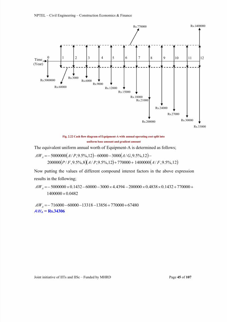
8/15/2019 2 Comparision of Alternatives
http://slidepdf.com/reader/full/2-comparision-of-alternatives 45/107
NPTEL – Civil Engineering – Construction Economics & Finance
Joint initiative of IITs and IISc – Funded by MHRD Page 45 of 107
Fig. 2.22 Cash flow diagram of Equipment-A with annual operating cost split into
uniform base amount and gradient amount
The equivalent uniform annual worth of Equipment-A is determined as follows;
12%,5.9,/140000077000012%,5.9,/8%,5.9,/200000
12%,5.9,/30006000012%,5.9,/5000000
F A P A F P
G A P A AW A
Now putting the values of different compound interest factors in the above expression
results in the following;
0482.01400000
7700001432.04838.02000004394.43000600001432.05000000 A AW
67480770000138561331860000716000
A AW AW A = Rs.34306
Rs.27000
Rs.60000
Rs.3000Rs.6000
Rs.9000Rs.12000
Rs.15000
Rs.18000Rs.21000
Rs.24000
Time(Year)
Rs.5000000
2 31 4 50 6 7 1098
Rs.770000
11 12
Rs.30000
Rs.1400000
Rs.200000
Rs.33000

8/15/2019 2 Comparision of Alternatives
http://slidepdf.com/reader/full/2-comparision-of-alternatives 46/107
NPTEL – Civil Engineering – Construction Economics & Finance
Joint initiative of IITs and IISc – Funded by MHRD Page 46 of 107
The cash flow diagram of Equipment-B is shown in Fig. 2.23.
Fig. 2.23 Cash flow diagram of Equipment-B
For Equipment-B, the annual income is in the form of a positive uniform gradient series
with gradient starting from end of year „ 6 . T he annual income is split into the uniform
base amount of Rs.710000 and the gradient amount in multiples of Rs.5000 starting from
end of year „ 6 till the end of useful life as shown in Fig. 2.24.
Fig. 2.24 Cash flow diagram of Equipment-B with annual income split into uniform base amount and gradient amount
Rs.230000
Rs.730000Rs.735000
Rs.715000
Rs.75000
Rs.720000Rs.725000
Time(Year)
Rs.4600000
2 31 4 50 6 7 1098
Rs.710000
11 12
Rs.740000
Rs.745000
Rs.1200000
Rs.75000
Time(Year)
Rs.4600000
2 31 4 50 6 7 1098
Rs.710000
11 12
Rs.20000Rs25000
Rs.5000Rs.10000
Rs.15000
Rs.30000Rs.35000
Rs.1200000
Rs.230000

8/15/2019 2 Comparision of Alternatives
http://slidepdf.com/reader/full/2-comparision-of-alternatives 47/107
NPTEL – Civil Engineering – Construction Economics & Finance
Joint initiative of IITs and IISc – Funded by MHRD Page 47 of 107
For the gradient series (of annual income), the equivalent present worth will be located at
the end of year „4 i.e. 2 years before the start of the gradient. The n the present worth of
this amount at time „0 will be c alculated and after that the equivalent annual worth of
this amount will be determined.
The equivalent uniform annual worth of Equipment-B is determined as follows;
12%,5.9,/120000012%,5.9,/4%,5.9,/8%,5.9,/5000710000
12%,5.9,/6%,5.9,/2300007500012%,5.9,/4600000
F A P A F P G P
P A F P P A AW B
Now putting the values of different compound interest factors in the above expression;
0482.012000001432.06956.04510.165000
7100001432.05801.0230000750001432.04600000 B AW
5784081937100001910675000658720
B AW AW B = Rs.23207
From the comparison by annual worth method, it is observed that Equipment-A exhibits
higher positive equivalent uniform annual worth as compared to Equipment-B. Thus the
Equipment-A is the most economical alternative.
Example -13
Using the annual worth method, compare the following machines having different life
spans at an interest rate of 11.5% per year.Machine-1
Cash flow details:
Initial purchase price = Rs.1200000
Annual operating cost = Rs.38000
Annual revenue = Rs.210000 for first 6 years and then Rs.225000 afterwards till the end
of useful life.
Expected salvage value = Rs.320000
Useful life = 14 years
Machine-2
Cash flow details:
Initial purchase price = Rs.1400000
Annual operating cost = Rs.26000

8/15/2019 2 Comparision of Alternatives
http://slidepdf.com/reader/full/2-comparision-of-alternatives 48/107
NPTEL – Civil Engineering – Construction Economics & Finance
Joint initiative of IITs and IISc – Funded by MHRD Page 48 of 107
Annual revenue = Rs.290000
Expected salvage value = Rs.450000
Useful life = 7 years
Solution:
The cash flow diagram of Machine-1 is shown in Fig. 2.25.
Fig. 2.25 Cash flow diagram of Machine-1
It may be noted here that the annual revenue is in the form of two uniform annual amount
series i.e. one with annual amount of Rs.21 0000 from beginning till end of year „6 and
the second one with annual amount of Rs.22 5000 from end of year „7 till the end of
useful life (as shown in Fig. 2.25). The annual revenue in the cash flow diagram can also
be represented as annual amount of Rs.210000 from beginning till the end of useful life
and the annual amount of Rs.15000 from end of year „7 till the end of useful lif e as
shown in Fig. 2.26.
Fig. 2.26 Cash flow diagram of Machine-1 with simplified representation of annual revenue
Time(Year)
Rs.1200000
2 31 4 50 6 7 1098
Rs.320000
11 12
Rs.210000
13 14
Rs.225000
Rs.38000
Time(Year)
Rs.1200000
2 31 4 50 6 7 1098
Rs.320000
11 12
Rs.210000
13 14
Rs.15000
Rs.38000
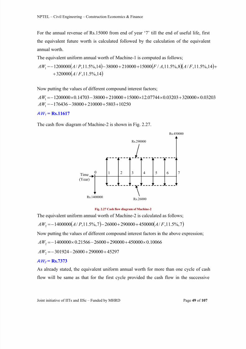
8/15/2019 2 Comparision of Alternatives
http://slidepdf.com/reader/full/2-comparision-of-alternatives 49/107
NPTEL – Civil Engineering – Construction Economics & Finance
Joint initiative of IITs and IISc – Funded by MHRD Page 49 of 107
For the annual revenue of Rs.15000 from end of year „7 till the end of useful life, first
the equivalent future worth is calculated followed by the calculation of the equivalent
annual worth.
The equivalent uniform annual worth of Machine-1 is computed as follows;
14%,5.11,/320000
14%,5.11,/8%,5.11,/150002100003800014%,5.11,/12000001
F A
F A A F P A AW
Now putting the values of different compound interest factors;
03203.032000003203.007744.12150002100003800014703.012000001 AW
102505803210000380001764361 AW
AW 1 = Rs.11617
The cash flow diagram of Machine-2 is shown in Fig. 2.27.
Fig. 2.27 Cash flow diagram of Machine-2
The equivalent uniform annual worth of Machine-2 is calculated as follows;
7%,5.11,/450000290000260007%,5.11,/14000002 F A P A AW
Now putting the values of different compound interest factors in the above expression;
10066.04500002900002600021566.014000002
AW 45297290000260003019242
AW
AW 2 = Rs.7373
As already stated, the equivalent uniform annual worth for more than one cycle of cash
flow will be same as that for the first cycle provided the cash flow in the successive
Time(Year)
Rs.1400000
2 31 4 50 6 7
Rs.450000
Rs.290000
Rs.26000

8/15/2019 2 Comparision of Alternatives
http://slidepdf.com/reader/full/2-comparision-of-alternatives 50/107
NPTEL – Civil Engineering – Construction Economics & Finance
Joint initiative of IITs and IISc – Funded by MHRD Page 50 of 107
cycles is exactly same as that in the first cycle. For illustration of this note, the cash flow
of Machine-2 is repeated for two cycles with life span of 7 years each (least common
multiple of life spans of the alternatives is 14 years).
The cash flow diagram of Machine-2 for two cycles is shown in Fig. 2.28
Fig. 2.28 Cash flow diagram of Machine-2 repeated for two cycles
The equivalent uniform annual worth of Machine-2 is determined as follows;
14%,5.11,/45000014%,5.11,/7%,5.11,/1400000
14%,5.11,/7%,5.11,/4500002900002600014%,5.11,/14000002
F A P A F P
P A F P P A AW
Now putting the values of different compound interest factors in the above expression
results in the following;
03203.045000014703.046674.01400000
14703.046674.04500002900002600014703.014000002 AW
03203.0450000
14703.046674.045000014000002900002600014703.014000002 AW
1441465194290000260002058422
AW AW 2 = Rs.7378
Now it can be seen that, the calculated equivalent uniform annual worth of Machine-2 for
two cycles of cash flow is same as that with only one cycle i.e. first cycle. The minor
difference among the values is due to the effect of decimal points in the above
calculations.
Time(Year)
Rs.1400000
2 31 4 50 6 7 1098
Rs.450000
11 12
Rs.290000
13 14
Rs.26000
Rs.450000
Rs.1400000

8/15/2019 2 Comparision of Alternatives
http://slidepdf.com/reader/full/2-comparision-of-alternatives 51/107
NPTEL – Civil Engineering – Construction Economics & Finance
Joint initiative of IITs and IISc – Funded by MHRD Page 51 of 107
Lecture-8
Rate of return:-
The rate of return technique is one of the methods used in selecting an alternative for a
project. In this method, the interest rate per interest period is determined, which equates
the equivalent worth (either present worth, future worth or annual worth) of cash
outflows (i.e. costs or expenditures) to that of cash inflows (i.e. incomes or revenues) of
an alternative. The rate of return is also known by other names namely internal rate of
return (IRR), profitability index etc. It is basically the interest rate on the unrecovered
balance of an investment which becomes zero at the end of the useful life or the study
period. In the following lectures, the rate of return is denoted by “ ir ” .
Using present worth, the equation for rate of return can be written as follows;
I C PW PW ……………………………… (2.1)
PW C = Present worth of cash outflows (cost or expenditure)
PW I = Present worth of cash inflows (income or revenue)
As already stated in earlier lectures, cost or expenditures are considered as negative cash
flows whereas income or revenues are considered as positive cash flows.
Equation (2.1) can be rewritten as;
I C PW PW 0 ………………………….. (2.2)
In the above equation the net present worth is zero.
Now putting the expressions for present worth of cash outflows and that of cash inflows
in equation (2.1) results in the following expression;
ni A P Ani F P F ni A P Ani F P F P r I r I r C r C o ,,/,,/,,/,,/ ……………. (2.3)
On left hand side of the above equation, P o is the initial cost at time zero and F C (single
amount) and AC (uniform amount series) are the expenditures occurring at future period
of time. Similarly on the right hand side of the equation, F I (single amount) and A I
(uniform amount series) are the incomes or revenues occurring at future period of time.
The value of interest period „n will vary depending upon the occurrence of the future
amounts (either expenditure or income).

8/15/2019 2 Comparision of Alternatives
http://slidepdf.com/reader/full/2-comparision-of-alternatives 52/107
NPTEL – Civil Engineering – Construction Economics & Finance
Joint initiative of IITs and IISc – Funded by MHRD Page 52 of 107
Equation (2.3) can be rewritten as follows;
ni A P Ani F P F ni A P Ani F P F P r I r I r C r C o ,,/,,/,,/,,/0 ……………..
(2.4)
The value of rate of return „ ir ’ can be calculated by solving the above equation. The
equation (2.4) can be solved either manually through trial and error process or using
Microsoft Excel spreadsheet. The first method i.e. trial and error process for
determination of the rate of return consumes more time whereas the second method is
faster. However the trial and error method gives a clear understanding of the analysis of
calculation for the rate of return. Similar to equivalent present worth, the rate of return
can also be determined by finding out the interest rate at which the net future worth or net
annual worth is zero.After determination of the rate of return for a given alternative, it is compared with
minimum attractive rate of return (MARR) to find out the acceptability of this alternative
for the project. If the rate of return i.e. ir is greater than or equal to MARR, then the
alternative will be selected or else it will not be selected. The MARR is the minimum rate
of return from the investment, which is acceptable. In other words it is the minimum rate
of return below which the investment alternatives are economically not acceptable. The
minimum attractive rate of return (MARR) serves as an important criteria while selecting
a single alternative or comparing mutually exclusive alternatives whenever the
investments are made. For an organization, it is governed by various parameters namely
availability of financially viable projects, amount of fund available for investment along
with the associated risk, and type of organization (i.e. government, public sector, private
sector etc.).
The difference between equivalent worth methods (present worth method/future worth
method/annual worth method) and rate of return method is that; in case of former, the
equivalent worth of the cash inflows and cash outflows are determined at MARR whereas
in case of latter, a rate is determined which equates the equivalent worth of cash inflows
to that of the cash outflows and the resulting rate is compared against MARR. The rate of
return and MARR are expressed in terms of percentage per period i.e. mostly percentage
per year.

8/15/2019 2 Comparision of Alternatives
http://slidepdf.com/reader/full/2-comparision-of-alternatives 53/107
NPTEL – Civil Engineering – Construction Economics & Finance
Joint initiative of IITs and IISc – Funded by MHRD Page 53 of 107
In the following example, the illustration of the procedure for determination of rate of
return for an alternative is presented.
Example -14A construction firm is planning to invest Rs.800000 for the purchase of a construction
equipment which will generate a net profit of Rs.140000 per year after deducting the
annual operating and maintenance cost. The useful life of the equipment is 10 years and
the expected salvage value of the equipment at the end of 10 years is Rs.200000.
Compute the rate of return using trial and error method based on present worth, if the
construction firm s minimum attractive rate of return (MARR) is 10% per year.
Solution:
The cash flow diagram of the construction equipment is shown in Fig. 2.29.
Fig. 2.29 Cash flow diagram of the construction equipment
For determination of rate of return „ir of the construction equipment, first the equation
for net present worth of cash inflows and cash outflows is equated to zero. Then using the
trial and error method the value of „i r is determined . The net present worth of cash
inflows and cash outflows of the construction equipment is given by the following
expression. 10,,/20000010,,/140000800000 r r i F P i A P PW
For determining the value of „i r the net present worth is equated to zero.
10,,/20000010,,/1400008000000 r r i F P i A P
Now the above equation will be solved through trial and error process to find out the
value of i r . Basically a positive value and a negative value of the net present worth will be
Time (Year)2 31 4 50
Rs.200000
6 7 1098
Rs.140000
Rs.800000

8/15/2019 2 Comparision of Alternatives
http://slidepdf.com/reader/full/2-comparision-of-alternatives 54/107
NPTEL – Civil Engineering – Construction Economics & Finance
Joint initiative of IITs and IISc – Funded by MHRD Page 54 of 107
determined at rate of return values close to the actual one and then by linear interpolation
between these two values, the actual rate of return will be calculated. For finding out the
rate of return values (close to the actual one), those will give a positive value and a
negative value of net present worth, one has to carry out a number of trial calculations at
various values of i r .
Since MARR is 10%, first assume a value of i r equal to 8% and compute the net present
worth. Now putting the values of different compound interest factors in the expression for
net present worth at i r equal to 8% results in the following;
10%,8,/20000010%,8,/140000800000 F P A P PW
4632.02000007101.6140000800000 PW
PW = Rs.232054
The above calculated net present worth at i r equal to 8% is greater than zero, now assume
a higher value of i r i.e. 12% for the next trial and compute the net present worth.
10%,12,/20000010%,12,/140000800000 F P A P PW
3220.02000006502.5140000800000 PW
PW = Rs.55428
As observed from this calculation, the net present worth is decreased at higher value of i r .
Thus for getting a negative value of net present worth, assume further higher value of i r
than the previous trial and take 14% for the next trial and determine the net present
worth.
10%,14,/20000010%,14,/140000800000 F P A P PW
2697.02000002161.5140000800000 PW
PW = -Rs.15806
Since a negative value of net present worth at i r equal to 14% is obtained (as above), theactual value of rate of return is less than 14%. The actual rate of return is now obtained
by doing linear interpolation either between 8% and 14% or between 12% and 14%.
However for obtaining a more accurate value of rate of return, the linear interpolation is
carried out between 12% and 14% and is given as follows;

8/15/2019 2 Comparision of Alternatives
http://slidepdf.com/reader/full/2-comparision-of-alternatives 55/107
NPTEL – Civil Engineering – Construction Economics & Finance
Joint initiative of IITs and IISc – Funded by MHRD Page 55 of 107
PW = Rs.55428 at i r = 12%
PW = - Rs.15806 at i r = 14%
%12
055428
%12%14
1580655428
r i
On solving the above expression, the value of i r is found to be 13.55% per year which is
greater than MARR (10%). Now using the using Microsoft Excel spreadsheet and
entering year-wise cash inflows and cash out flows, the value of rate of return is found to
be 13.53% (using the function „IRR ). However this minor difference in the value of i r
obtained from both the methods can be minimized by finding out the net present worth at
narrow range of interest rate values and carrying out linear interpolation between these
values (trial and error method) to find out the more precise value close to the actual rate
of return.
The net present worth of the construction equipment at MARR i.e. 10% is given by;
10%,10,/20000010%,10,/140000800000 F P A P PW
3855.02000001446.6140000800000 PW
PW = Rs.137344 at MARR (10%)
The net present worth of the construction equipment at MARR is greater than zero and
the rate of return is greater than MARR. Thus the purchase of the construction equipment
is economically justified. It may be noted here that when the equivalent worth of an
investment is greater than zero at interest rate equal to MARR, then the rate of return of
the investment is greater than MARR.
12% 13% 14%
55428
-15806
PW (Rs.)
ir

8/15/2019 2 Comparision of Alternatives
http://slidepdf.com/reader/full/2-comparision-of-alternatives 56/107
NPTEL – Civil Engineering – Construction Economics & Finance
Joint initiative of IITs and IISc – Funded by MHRD Page 56 of 107
The rate of return „i r can also be determined by equating the net annual worth to zero.
For the above construction equipment, the net equivalent annual worth at different values
of i r are calculated as follows;
At i r = 12%
10%,12,/20000014000010%,12,/800000 F A P A AW
0570.02000001400001770.0800000 AW
AW = Rs.9800
At i r = 14%
10%,14,/20000014000010%,14,/800000 F A P A AW
0517.02000001400001917.0800000 AW
AW = -Rs.3020 Now carrying out the linear interpolation between 12% and 14%;
AW = Rs.9800 at i r = 12%
AW = - Rs.3020 at i r = 14%
%1209800
%12%1430209800
r i
On solving the above expression, the value of i r is found to be 13.52% per year. Theminor difference in the values of i r from present worth and annual worth methods is due
to the effect of decimal points in the calculations. Similar to present worth and annual
worth methods, t he rate of return „i r can also be determined by equating the net future
worth to zero.
AW (Rs.)
12% 13% 14%
9800
-3020
ir

8/15/2019 2 Comparision of Alternatives
http://slidepdf.com/reader/full/2-comparision-of-alternatives 57/107
NPTEL – Civil Engineering – Construction Economics & Finance
Joint initiative of IITs and IISc – Funded by MHRD Page 57 of 107
From the above example, a unique value of rate of return was obtained for the
construction equipment (on the basis of its cash inflow and cash outflow). This is due to
the fact that, there was only one sign change in the cash flows i.e. minus sign at time zero
for the cash outflow followed by plus sign for cash inflows during the remaining periods.
However in some cases, depending upon the cash flow it is possible to get multiple
values of rate of return, those satisfy the rate of return equation of the equivalent worth of
cash inflows and cash out flows. This may happen due to more than one sign change in
the cash flows e.g. cash outflow (negative) at beginning (time zero) followed cash
inflows (positive) at end of year 1 and 2 and then cash outflow (negative) at end of year 3
etc. Thus while selecting an alternative that has multiple values of rate of return
(depending on the cash flow), other method of economic evaluation may be adopted to
find out the economical suitability of the alternative.

8/15/2019 2 Comparision of Alternatives
http://slidepdf.com/reader/full/2-comparision-of-alternatives 58/107
NPTEL – Civil Engineering – Construction Economics & Finance
Joint initiative of IITs and IISc – Funded by MHRD Page 58 of 107
Lecture-9Incremental Rate of return:-
When the best alternative (economically suitable) is to be selected from two or more
mutually exclusive alternatives on the basis of rate of return analysis, the incremental
investment analysis is used. In incremental rate of return method, the alternative with
larger investment is selected, provided the incremental (extra) investment over the lower
investment alternative produces a rate of return that is greater than or equal to MARR. In
other words if the additional benefits i.e. increased productivity, increased income,
reduced operating expenditure etc. achieved at the expense of extra investment
(associated with larger investment alternative) are more than that could have been
obtained from the investment of same amount at MARR elsewhere by the organization,
then this additional capital should be invested.
In incremental rate of return method, the economically acceptable lower investment
alternative is considered as the base alternative against which the higher investment
alternative is compared. The cash flow of higher investment alternative is considered
equal to the cash flow of lower investment alternative plus the incremental cash flow i.e.
difference in cash flow between the higher investment and lower investment alternatives.
When using rate of return method for comparing two or more mutually exclusive
alternatives, the analysis must be done correctly, otherwise it may lead to incorrect
ranking of the alternatives. However this problem is avoided in incremental investment
rate of return analysis. In this technique, the individual rate of return values on total cash
flow of the mutually exclusive alternatives are not compared against each other rather the
rate of return (or IRR) of the mutually exclusive alternatives or the rate of return of the
incremental investment is compared against MARR.
The procedures for comparison of mutually exclusive cost alternatives and that of
mutually exclusive investment alternatives using incremental investment rate of returnanalysis are mentioned below. The details about cost and investment alternatives are
already stated in Lecture-1 of Module 2.

8/15/2019 2 Comparision of Alternatives
http://slidepdf.com/reader/full/2-comparision-of-alternatives 59/107
NPTEL – Civil Engineering – Construction Economics & Finance
Joint initiative of IITs and IISc – Funded by MHRD Page 59 of 107
Steps for comparison of cost alternatives:
i) First arrange the mutually exclusive cost alternatives on the basis of increasing initial
capital investment. The lowest capital investment alternative is considered as the base
alternative (B).
ii) The incremental cash flow is calculated between the base alternative (B) and the next
higher capital investment alternative (H) over the useful life.
iii) Then the rate of return „ir(H-B) of this incremental investment is calculated (procedure
as stated earlier) by equating the net equivalent worth (present worth or annual worth or
future worth) to zero.
iv) If the calculated „ir(H-B) is greater than or equal to MARR, then alternative „B is
removed from further analysis. A lternative „ H now becomes the new base alternative
and is compared against the next higher capital investment alternative . If „i r(H-B) is less
than MARR, then alternative „H is removed from further analysis and alternative „B
remains as the base alternative and is compared against the next higher investment
alternative (alternative with investment higher than „H ) .
v) Steps ii) to iv) are repeated till only one alternative is left i.e. the best alternative which
justifies the incremental investment associated with.
Steps for comparison of investment alternatives:i) Arrange the mutually exclusive investment alternatives on the basis of increasing initial
capital investment.
ii) Then the rate of return (IRR) on total cash flow of the lowest investment alternative is
determined (procedure already stated earlier) to find out its acceptability as the base
alternative. If the calculated rate of return is greater than or equal to MARR, this is
selected as the base alternative. If the calculated rate of return is less than MARR, then
this alternative is not considered for further analysis and the acceptability of the next
higher investment alternative as base alternative is found out by calculating the rate of
return on its total cash flow and comparing against MARR. This process is continued till
the base alternative „B (acceptab le alternative for which rate of return greater than or
equal to MARR) is obtained. If no alternative is obtained in this manner i.e. rate of return
less than MARR, then do-nothing alternative is selected. The do-nothing alternative

8/15/2019 2 Comparision of Alternatives
http://slidepdf.com/reader/full/2-comparision-of-alternatives 60/107
NPTEL – Civil Engineering – Construction Economics & Finance
Joint initiative of IITs and IISc – Funded by MHRD Page 60 of 107
indicates that all the investment alternatives are rejected. Similar to the comparison of
cost alternatives, the incremental cash flow is now calculated between the base
alternative (B) and the next higher investment alternative (H) over the useful life.
Steps iii) to v) as mentioned above for the comparison of cost alternatives are then
followed to select the best alternative.
The comparison of cost alternatives is illustrated in the following example.
Example -15
The development authority of a city has to select a pumping unit from four feasible
mutually exclusive alternatives for supply of water to a particular location of the city. The
details of cash flow and the useful life of all the alternatives are presented in the
following table. The minimum attractive rate of return (MARR) is 20% per year. Selectthe best alternative using the incremental investment rate of return analysis.
Solution:
The cash flow and useful life of all the alternatives are presented in Table 2.1.
Table 2.1 Cash flow of alternatives
Alternative
Cash flow
Alternative-1A1
Alternative-2A2
Alternative-3A3
Alternative-4A4
Initial capitalinvestment (Rs.)
7800000 6600000 8100000 7400000
Annual operating andmaintenance cost (Rs.)
850000 1185000 800000 970000
Salvage value (Rs.) 2050000 1780000 2200000 1865000
Useful life (Years) 10 10 10 10
As seen from the above table, these are cost alternatives involving all cash outflows
(negative cash flows) except for the salvage value (positive cash flow) at the end of
useful life. The alternatives are not in the increasing order of capital investment as

8/15/2019 2 Comparision of Alternatives
http://slidepdf.com/reader/full/2-comparision-of-alternatives 61/107
NPTEL – Civil Engineering – Construction Economics & Finance
Joint initiative of IITs and IISc – Funded by MHRD Page 61 of 107
observed from Table 2.1. The alternatives are now arranged in the increasing order of
capital investment as shown in Table 2.2 and cash outflows and cash inflows are shown
with negative and positive signs respectively.
Table 2.2 Cash flow of alternatives in increasing order of initial capital investment
Alternative
Cash flow
Alternative-2
A2
Alternative-4
A4
Alternative-1
A1
Alternative-3
A3
Initial capital
investment (Rs.)-6600000 -7400000 -7800000 -8100000
Annual operating and
maintenance cost (Rs.)-1185000 -970000 -850000 -800000
Salvage value (Rs.) +1780000 +1865000 +2050000 +2200000
Useful life (Years) 10 10 10 10
After arranging the alternatives in increasing order of capital investment, alternative-2
(A2) now becomes the base alternative (lowest capital investment with Rs.6600000) and
it is compared with the next higher investment alternative i.e. alternative-4 (A4) withcapital investment of Rs.7400000. The incremental cash flow between the two
alternatives A2 and A4
is given as follows;
Incremental capital investment = -Rs.7400000 – (-Rs.6600000) = -Rs.800000 at
beginning i.e. at time zero.
Incremental annual operating and maintenance cost from end of year 1 till end of year 10
= -Rs.970000 – (-Rs.1185000) = Rs.215000
Incremental salvage value = Rs.1865000 – Rs.1780000 = Rs.85000 at end of year 10
In order to find out the rate of return (IRR) of this incremental cash flow, the net present
worth is equated to zero.
10,,/8500010,,/2150008000000 r r i F P i A P PW

8/15/2019 2 Comparision of Alternatives
http://slidepdf.com/reader/full/2-comparision-of-alternatives 62/107
NPTEL – Civil Engineering – Construction Economics & Finance
Joint initiative of IITs and IISc – Funded by MHRD Page 62 of 107
The value of rate of return „ ir ’ is now calculated by solving the above equation either
manually through trial and error process with linear interpolation or using Microsoft
Excel spreadsheet (already mentioned earlier). For faster calculation, the rate of return is
calculated using Microsoft Excel spreadsheet after entering year-wise cash inflows and
cash out flows. The value of rate of return is found to be 24.06% (using the function
„IRR in Excel spreadsheet). As rate of return of the incremental cash flow is greater than
MARR (20%), the incremental investment associated with alternative-4 (A4) is justified
and alternative-2 (A2) is now removed from further analysis. Alternative-4 now becomes
the new base alternative and is compared with next higher capital investment alternative
i.e. alternative-1 (A1) with investment of Rs.7800000. The rate return of this incremental
investment is calculated in same manner as above. The entire calculation is now
presented in the Table 2.3.
Table 2.3 Comparison of cost alternatives using incremental rate of return analysis
Comparison
Incremental cash flow
BetweenA4 and A2
BetweenA1 and A4
BetweenA3 and A1
Incremental capital investment(Rs.)
-800000 -400000 -300000
Incremental annual operating and
maintenance cost i.e. savings (Rs.)
215000 120000 50000
Incremental salvage value (Rs.) 85000 185000 150000
Useful life (Years) 10 10 10
Rate of return on incrementalinvestment
24.06%( > MARR)
28.65%( > MARR)
14.09%( < MARR)
Incremental investment justified Yes Yes No
Present worth of incremental cashflow at MARR, 20% (Rs.)
115115 ( > 0) 132978 ( > 0) -66150 ( < 0)
In Table 2.3 the incremental values between the alternatives indicate the difference in
cash flows between them.

8/15/2019 2 Comparision of Alternatives
http://slidepdf.com/reader/full/2-comparision-of-alternatives 63/107
NPTEL – Civil Engineering – Construction Economics & Finance
Joint initiative of IITs and IISc – Funded by MHRD Page 63 of 107
The outcomes of the incremental investment analysis for the comparison of cost
alternatives as presented in Table 2.3 are briefly described below.
Comparison between alternatives A2 (base alternative) and A4 (next higher capital
investment alternative). The obtained rate of return form the incremental investment
analysis is 24.06% which is greater than MARR (20%). Alternative-2 (A2) is
eliminated from further analysis and alternative-4 (A4) is the new base alternative.
Now comparison between alternatives A4 and A1 (next higher capital investment
alternative). The obtained rate of return form the incremental investment is 28.65%
and is greater than MARR. Thus alternative-4 (A4) is eliminated from further
analysis and alternative-1 (A1) is the new base alternative.
Finally comparison between alternatives A1 and A3 (next higher capital investmentalternative). The rate of return obtained from the incremental investment analysis is
14.09% which is less than MARR (20%). Thus the incremental investment
associated with alternative-3 (A3) i.e. largest capital investment alternative is not
justified and hence alternative-1 (A1) is selected as the best alternative, as no
other alternative is left for comparison . In addition, the present worth of the
incremental investment associated with alternative-1 (A1) over alternative-4 (A4) at
MARR i.e. 20% is greater than zero i.e. Rs.132978 > 0.
It can be seen here that, the largest capital investment alternative (A3) is not selected
because the incremental investment associated with it results in a rate of return
which is less than MARR. In addition the present worth of the incremental
investment associated with alternative-3 (A3) over alternative-1 (A1) at MARR i.e.
20% is less than zero i.e. – Rs.66150 < 0.
Now the values of equivalent present worth of the total cash flow of the cost alternatives
at MARR (20%) are found to be -Rs.11280643, -Rs.11165528, -Rs.11098700 and -Rs.11032550 for alternatives A2, A4, A3 and A1 respectively. Thus alternative A1 (the
best alternative) exhibits lowest negative equivalent present worth as compared to other
cost alternatives.

8/15/2019 2 Comparision of Alternatives
http://slidepdf.com/reader/full/2-comparision-of-alternatives 64/107
NPTEL – Civil Engineering – Construction Economics & Finance
Joint initiative of IITs and IISc – Funded by MHRD Page 64 of 107
Lecture-10
Incremental Rate of return:-
The comparison of investment alternatives using incremental investment rate of returnanalysis is illustrated in the following example.
Example -16
A construction company is planning to invest for the purchase of a heavy construction
equipment which will be used at a construction site. There are four feasible alternatives
and the detailed cash flow of all the alternatives are presented in Table 2.4. Each
alternative has the useful life of 8 years. If the co mpany s MARR is 12% per year, select
the best alternative using the incremental investment rate of return analysis.
Solution:
The cash flow and useful life of all the alternatives are presented in Table 2.4.
Table 2.4 Cash flow of alternatives
Alternative
Cash flow
Alternative-1
B1
Alternative-2
B2
Alternative-3
B3
Alternative-4
B4
Initial investment (Rs.) 2400000 3400000 2700000 3200000
Annual profit (after deductingexpenditures) (Rs.)
415000 680000 525000 640000
Salvage value (Rs.) 590000 990000 710000 860000
Useful life (Years) 8 8 8 8
As observed from Table 2.4, these are investment alternatives having positive cash flows
(cash inflows). As the alternatives are not in the increasing order of investment, they are
now arranged in the increasing order of investment as shown in Table 2.5.

8/15/2019 2 Comparision of Alternatives
http://slidepdf.com/reader/full/2-comparision-of-alternatives 65/107
NPTEL – Civil Engineering – Construction Economics & Finance
Joint initiative of IITs and IISc – Funded by MHRD Page 65 of 107
Table 2.5 Cash flow of alternatives in increasing order of investment
Alternative
Cash flow
Alternative-1
B1
Alternative-3
B3
Alternative-4
B4
Alternative-2
B2
Initial investment (Rs.) -2400000 -2700000 -3200000 -3400000
Annual profit (after deductingexpenditures) (Rs.)
415000 525000 640000 680000
Salvage value (Rs.) 590000 710000 860000 990000
Useful life (Years) 8 8 8 8
After arranging the alternatives in increasing order of investment, the acceptability of the
lowest investment alternative i.e. alternative B1 as base alternative is checked by finding
out the rate of return on its total cash flow. The rate of return is found out by equating net
present worth of alternative B1 to zero.
8,,/5900008,,/41500024000000 r r i F P i A P PW
As already stated, the value of rate of return „ir ’ is calculated by solving the above
equation either manually through trial and error process with linear interpolation or usingMicrosoft Excel spreadsheet. The value of rate of return is found to be 10.91% (using the
function „IRR in Excel spreadshe et), which is less than company s MARR i.e. 12%.
Thus alternative B1 is eliminated from further calculation and the acceptability of next
higher investment alternative i.e. B3 is checked in the same manner as above. The rate of
return on total cash flow of alternative B3 is determined by equating the net present
worth to zero.
8,,/7100008,,/52500027000000 r r i F P i A P PW
From this equation the value of rate of return is found to be 13.84% (using the function
„IRR in Excel spreadsheet), which is greater than company s MARR i.e. 12%. Thus
Alternative B3 becomes the base alternative and it is compared with the next higher
investment alternative B4. Now the rate of return of the incremental cash flow between

8/15/2019 2 Comparision of Alternatives
http://slidepdf.com/reader/full/2-comparision-of-alternatives 66/107
NPTEL – Civil Engineering – Construction Economics & Finance
Joint initiative of IITs and IISc – Funded by MHRD Page 66 of 107
the two alternatives B3 and B4 is calculated and compared with MARR to check
suitability of the incremental investment associated with alternative B4. The entire
calculation for selecting the best alternative is now presented in Table 2.6.
Table 2.6 Comparison of investment alternatives using incremental rate of return analysis
Alternatives
Cash flowB1 B3 B4 – B3 B2 – B4
Initial investment / Incremental value (Rs.) -2400000 -2700000 -500000 -200000
Annual profit (after deducting expenditures) /Incremental value (Rs.)
415000 525000 115000 40000
Salvage / Incremental value (Rs.)590000 710000 150000 130000
Useful life (Years) 8 8 8 8
Rate of return on total cash flow / Rate ofreturn on incremental investment
10.91%( < MARR)
13.84%( > MARR)
18.52%( > MARR)
17.69%( > MARR)
Acceptable as base alternative / Incrementalinvestment justified
No Yes Yes Yes
Present worth of incremental cash flow atMARR 12% (Rs.)
- - 131859 ( > 0) 51211 ( > 0)
In the above table the incremental values between the alternatives indicate the difference
in their cash flows.
In Table 2.6, the total cash flows of the individual alternatives and incremental cash flows
(comparison between two alternatives) are written in different colour fonts for ease of
understanding. For alterative B1 and B3, total cash flows and for comparison between B4
– B3
and B2 – B4 the incremental cash flows are provided in the above table.

8/15/2019 2 Comparision of Alternatives
http://slidepdf.com/reader/full/2-comparision-of-alternatives 67/107
NPTEL – Civil Engineering – Construction Economics & Finance
Joint initiative of IITs and IISc – Funded by MHRD Page 67 of 107
The outcomes of the incremental investment analysis for comparison of investment
alternatives (presented in Table 2.6) are briefly described below.
Checking the acceptance of lowest investment alternative B1 as base alternative by
calculating the rate of return on its total cash flow. The obtained rate of return is
10.91% which is less than MARR (12%). Alternative B1 is now eliminated from
further analysis.
Now checking the acceptance of next higher investment alternative B3 as the base
alternative by finding out the rate of return on its total cash flow. The obtained rate
of return is 13.84% which is greater than MARR (12%). Thus alternative B3 now
becomes the base alternative.
Now comparison between alternatives B3 and next higher investment alternative B4 .
The rate of return form the incremental investment analysis is found to be 18.52%
which is greater than MARR (12%). Thus alternative B3 is eliminated from further
analysis and alternative B4 is the new base alternative as the incremental investment
is justified.
Finally comparison between alternatives B4 and B2 (next higher investment
alternative). The obtained rate of return from the incremental investment is 17.69%
which is greater than MARR (12%). Thus the incremental investment associated
with alternative B2 is justified and alternative B2 is selected as the bestalternative, as there is no other alternative remaining for comparison . Further the
present worth of the incremental investment associated with alternative B2 over
alternative B4 at MARR (12%) is greater than zero as observed from Table 2.6.
Now the values of equivalent present worth of the total cash flow of individual
alternatives at MARR (12%) are found to be -Rs.100145, Rs.194759, Rs.326618 and
Rs.377829 for alternatives B1, B3, B4 and B2 respectively. Thus alternative B2 exhibits
highest positive equivalent present worth as compared to other alternatives which is inagreement with outcome obtained from the incremental investment analysis.
For comparison of mutually exclusive alternatives, those have different life spans, the
comparison using incremental rate of return analysis must be made over the same number

8/15/2019 2 Comparision of Alternatives
http://slidepdf.com/reader/full/2-comparision-of-alternatives 68/107
NPTEL – Civil Engineering – Construction Economics & Finance
Joint initiative of IITs and IISc – Funded by MHRD Page 68 of 107
of years i.e. least common multiple of the individual life spans as in case of comparison
using present worth method in earlier lectures.
The important points to be noted for comparison of mutually exclusives alternatives usingincremental investment rate of return analysis are as follows.
The alternative with larger investment should be selected if the incremental (extra)
investment associated with it over the lower investment alternative produces a rate of
return that is greater than or equal to MARR.
While comparing the alternatives, at first instance the alternative with highest rate of
return on its total cash flow should not be selected as the best alternative. After
carrying out the incremental investment rate of return analysis, the selection of the
best alternative may match (depending on the cash flow) with the alternative with
highest rate of return on its total cash flow. The rate of return of the alternatives B1,
B2, B3 and B4 (Example 16) on their total cash flows are found to be 10.91%,
14.80%, 13.84% and 14.59% respectively (calculations not shown in the example).
Thus Alternative B2 having highest rate of return (also greater than MARR i.e.
14.80% > 12%) was not selected as the best alternative at first instance. However
from outcome of incremental investment rate of return analysis, alternative B2 was
selected as the best alternative that matched with the alternative having highest rate of
return.
Similarly the alternative with highest capital investment and has rate of return (on its
total cash flow) greater than or equal to MARR, should not be selected as the best
alternative at first instance. However the outcome of the incremental investment rate
of return analysis for the best alternative may coincide with the highest investment
alternative (with rate of return on its total cash flow greater than or equal to MARR).
From incremental investment rate of return analysis, alternative B2 (Example 16)
was selected as the best alternative, which happened to be the highest investment
alternative with rate of return on its total cash flow greater than MARR.

8/15/2019 2 Comparision of Alternatives
http://slidepdf.com/reader/full/2-comparision-of-alternatives 69/107
NPTEL – Civil Engineering – Construction Economics & Finance
Joint initiative of IITs and IISc – Funded by MHRD Page 69 of 107
The higher capital investment alternative associated with the incremental capital
investment that exhibits highest rate of return should not be selected as the best
alternative. As observed from Example 16, incremental investment having highest
rate of return (18.52%) was between alternatives B4 and B3 and the higher
investment alternative associated with this incremental investment was B4. On the
other hand, the rate of return on the incremental capital investment between B2 and
B4 was 17.69% and the higher investment alternative associated with this
incremental investment was B2. From the incremental rate of return analysis,
alternative B2 was selected as the best alternative in place of B4, even though the
rate of return on incremental investment associated with B4 (comparison between B4
and B3) was greater than the rate of return on the incremental investment associated
with B2 (comparison between B2 and B4) i.e. 18.52% > 17.69%.

8/15/2019 2 Comparision of Alternatives
http://slidepdf.com/reader/full/2-comparision-of-alternatives 70/107
NPTEL – Civil Engineering – Construction Economics & Finance
Joint initiative of IITs and IISc – Funded by MHRD Page 70 of 107
Lecture-11
Capitalized cost analysis:-
Capitalized cost represents the present worth of an alternative for a project that is going
to serve for a longer period of time i.e. for an infinite period of time. As the name
indicates, it refers to the present worth of mainly cost or expenditures (cash outflows) of
the alternative over infinite period of time. Capitalized worth refers to present worth of
expenditures and revenues of an alternative over infinite period of time.
The capitalized cost method is used for comparison of mutually exclusive alternatives
which have perpetual service life (assumed to serve forever). The examples of this kind
of projects are bridges, dams, irrigation projects, water supply systems for cities, pipeline
projects etc. This method an also be used for finding out the capitalized cost of permanent
fellowship/scholarship endowment in educational institutes and other organizations.
As already stated, capitalized cost/worth is the present worth of an alternative that has a
perpetual or permanent cash flow series. The capitalized cost/worth of a perpetual cash
flow having uniform amount series with end of year payments „A is obtained as follows.
The present worth of a uniform amount series is given by;
n
n
ii
i A P
1
11
P = present worth, A = end of year payment of uniform amount series, i = interest rate per
year and n = number of interest periods (already stated in Module 1)
The above equation can be rewritten as;
nn
n
ii
ii
A P
1
1
1
1
n
ii
A P
1
11
In the above expression, when „n approaches infinity (i.e. for perpetual cash flow series),
the term “1/(1+i) n” gets neglected and present worth „P becomes capitalized cost /worth,
the expression of which is given by;
i A
P

8/15/2019 2 Comparision of Alternatives
http://slidepdf.com/reader/full/2-comparision-of-alternatives 71/107
NPTEL – Civil Engineering – Construction Economics & Finance
Joint initiative of IITs and IISc – Funded by MHRD Page 71 of 107
i P A
Thus the above expression can be explained by a simple example.
If a person deposits an amount of Rs.100000 in a bank at an interest rate of 10% per year,
then how much money the person can withdraw from the bank every year without
reducing the original deposit.
- The amount of interest accumulated (i.e. amount of money the person can withdraw
without reducing the deposit) at the end of 1 st year is Rs.10000 (100000 x 0.10).
- After withdrawal of Rs.10000 at the end of 1 st year, the amount that will remain in his
bank account is Rs.100000, which will again earn an interest amount of Rs.10000 at the
end of 2 nd year. After withdrawal of Rs.10000 at the end of 2 nd year, the person will have
again the same amount of Rs.100000 in his bank account that will further earn the same
interest amount at the end of 3 rd year. This process can be continued perpetually
generating an interest amount of Rs.10000 (A = P x i) without changing the original
deposit of Rs.100000. This example is similar to creating a scholarship endowment in a
university that will give a scholarship of Rs.10000 every year indefinitely, by depositing
Rs.100000 in a saving bank account at interest rate of 10% per year compounded
annually.
The capitalized cost of a single amount occurring at regular intervals in future period of
time is calculated by first finding out the equivalent uniform annual worth „A of theuniform series and then dividing by the interest rate „i .
The calculation of capitalized cost of an alternative is illustrated in the following
example.
Example -17
A public project has an initial cost of Rs.11000000 and annual operating and maintenance
cost of Rs.700000. Further the project will have one time major repair work of
Rs.2000000 at the end of 15 year. Find out the capitalized cost of the alternative if
interest rate is 12% per year.
Solution:
The capitalized cost of the alternative is equal to sum of the initial cost, present worth of
one time major repair cost and capitalized cost of the annual operating and maintenance
cost.

8/15/2019 2 Comparision of Alternatives
http://slidepdf.com/reader/full/2-comparision-of-alternatives 72/107
NPTEL – Civil Engineering – Construction Economics & Finance
Joint initiative of IITs and IISc – Funded by MHRD Page 72 of 107
The total capitalized cost of the alternative is given by;
ini F P Cost d Capitalize 700000,,/200000011000000
12.070000015%,12,/200000011000000 F P Cost d Capitalize
58333331827.0200000011000000 Cost d Capitalize Capitalized cost = -Rs.17198733
Therefore the capitalized cost of the alternative for the public project is found to be
Rs.17198733.

8/15/2019 2 Comparision of Alternatives
http://slidepdf.com/reader/full/2-comparision-of-alternatives 73/107
NPTEL – Civil Engineering – Construction Economics & Finance
Joint initiative of IITs and IISc – Funded by MHRD Page 73 of 107
Lecture-12Capitalized cost analysis:-
The capitalized cost can also be used for comparison of two or more mutually exclusive
alternatives which are assumed to serve perpetually. In this case the comparison of the
alternatives is made over same time period i.e. infinite period of time. The alternative that
shows lowest capitalized cost is selected as the best alternative.
In the following examples, the calculation of capitalized cost of an alternative and the
comparison of mutually exclusive alternatives on the basis of capitalized cost are
illustrated.
Example -18
The initial cost of an infrastructure development project which is expected to serve
residents of a city perpetually is Rs.15000000. The annual operating cost is Rs.800000
for first 10 years and Rs.900000 in the subsequent years (i.e. from year 11 onwards). The
expected cost of renovation at the end of every 15 years is Rs.1800000. Find out the
capitalized cost of the project at interest rate of 8% per year.
Solution:
The cash flow diagram of the project for a part of service life is shown in Fig. 2.30
The total capitalized cost of the project is equal to sum of the initial cost and capitalized
cost of annual operating cost and renovation cost.
Fig. 2.30 Cash flow diagram of the project
The annual operating cost is Rs.800000 for first 10 years followed by Rs.900000
thereafter. This can be represented as Rs.800000 from end of year 1 to infinite period of
Time(Year)
Rs.15000000
2 31 4 50 6 7 1098 11 12 13 14
Rs.800000
Rs.100000
15 16
Rs.1800000
Time (year) approaching infinity

8/15/2019 2 Comparision of Alternatives
http://slidepdf.com/reader/full/2-comparision-of-alternatives 74/107
NPTEL – Civil Engineering – Construction Economics & Finance
Joint initiative of IITs and IISc – Funded by MHRD Page 74 of 107
time and Rs.100000 from end of year 11 to infinity as shown in Fig. 2.30. Thus the
capitalized cost of the annual operating cost is equal to the sum of capitalized cost of
these two components.
Capitalized cost of the annual operating cost:
10,,/100000800000
i F P ii
Cost d Capitalize
In the above expression, the capitalized cost of Rs.100000 from end of year 11 till
infinity is located at the end of year 10. Now the present worth (i.e. amount at time zero)
of this amount is calculated by multiplying it with single payment present worth factor.
10%,8,/08.0
10000008.0
800000 F P Cost d Capitalize
08.04632.0100000
10000000
Cost d Capitalize
Capitalized cost = -Rs.10579000
The capitalized cost of the annual operating cost can also be calculated by considering
Rs.800000 from end of year 1 till end of year 10 and Rs.900000 from end of year 11 till
infinity. The calculation is shown below.
10,,/900000
10,,/800000 i F P i
i A P Cost d Capitalize
In this expression, first the present worth of uniform series with annual amount ofRs.800000 for first 10 years is calculated. Then the capitalized cost of Rs.900000 from
end of year 11 till infinity is calculated in the same manner as for Rs.100000 in the first
approach.
10%,8,/08.0
90000010%,8,/800000 F P A P Cost d Capitalize
08.04632.0900000
7101.6800000
Cost d Capitalize
Capitalized cost = -Rs.10579080Thus it can be seen that the capitalized cost of annual operating cost by both ways is
same. The minor difference between the values is due to the effect of decimal points in
the calculations.

8/15/2019 2 Comparision of Alternatives
http://slidepdf.com/reader/full/2-comparision-of-alternatives 75/107
NPTEL – Civil Engineering – Construction Economics & Finance
Joint initiative of IITs and IISc – Funded by MHRD Page 75 of 107
Capitalized cost of renovation component:
The renovation will take place at the end of every 15 years i.e. at the end of 15 th year, 30 th
year, 45 th year etc. In order to calculate the capitalized cost of renovation component
(Rs.1800000) at the end of every 15 years, first the uniform annual amount „A of the
equivalent uniform series for the first 15 years is calculated. This amo unt „A will be
same for the subsequent intervals i.e. from end of year 16 till end of year 30, from end of
year 31 till end of till year 45 and so on (shown in Fig. 2.31). Then the uniform amount
„A is divided by the interest rate.
Fig. 2.31 Cash flow diagram for periodic renovation cost of the project
08.0
15%,8,/1800000 F ACost d Capitalize
08.00368.01800000
Cost d Capitalize
Capitalized cost = -Rs.828000
Now the total capitalized cost of the project is equal to initial cost plus capitalized cost of
annual operating cost and renovation cost.
Capitalized cost = -Rs.15000000 -Rs.10579000 -Rs.828000
Capitalized cost = -Rs.26407000Therefore the capitalized cost of the infrastructure development project is Rs.26407000.
TimeYear) 2 31 130
Rs.1800000
Time (year) approaching infinity
14 15 17 292816 3018
Rs.1800000
A
32 444331 33
Rs.18

8/15/2019 2 Comparision of Alternatives
http://slidepdf.com/reader/full/2-comparision-of-alternatives 76/107
NPTEL – Civil Engineering – Construction Economics & Finance
Joint initiative of IITs and IISc – Funded by MHRD Page 76 of 107
Example -19
There are two alternatives for a water supply project in a city. The details of cash flow of
the alternatives are shown below.
Alternative-1Initial cost = Rs.20000000
Annual operating cost = Rs.1600000
Cost of renovation = Rs.2500000 at the end of every 17 years
One time upgrading cost = Rs.3200000 at the end of 22 year
Alternative-2
Initial cost = Rs.26000000
Annual operating cost = Rs.1200000
Cost of renovation = Rs.3500000 at the end of every 20 years
Compare the alternatives on the basis of capitalized cost and find out the economical
alternative if the rate of interest is 9% per year
Solution:
The capitalized cost of Alternative-1 will be equal to initial cost plus the capitalized cost
of annual operating cost, periodic renovation cost and one time upgrading cost.
The capitalized cost of Alternative-1 is calculated as follows;
22,,/320000017,,/2500000160000020000000 i F P i
i F Ai
Cost d Capitalize
22%,9,/320000009.0
17%,9,/250000009.0
160000020000000 F P
F ACost d Capitalize
1502.0320000009.0
0270.025000001777777820000000 Cost d Capitalize
4806407500001777777820000000 Cost d Capitalize
Capitalized cost = -Rs.39008418 (Alternative-1)
The capitalized cost of Alternative-2 will be equal to initial cost plus the capitalized cost
of annual operating cost and periodic renovation cost.
The capitalized cost of Alternative-2 is obtained as follows;
i
i F Ai
Cost d Capitalize 20,,/35000001200000
26000000

8/15/2019 2 Comparision of Alternatives
http://slidepdf.com/reader/full/2-comparision-of-alternatives 77/107
NPTEL – Civil Engineering – Construction Economics & Finance
Joint initiative of IITs and IISc – Funded by MHRD Page 77 of 107
09.0
20%,9,/350000009.0
120000026000000
F ACost d Capitalize
09.00195.03500000
1333333326000000
Cost d Capitalize
7583331333333326000000 Cost d Capitalize
Capitalized cost = -Rs.40091666 (Alternative-2)
The capitalized cost of altenative-1 and Alternative-2 are found to be Rs.39008418 and
Rs.40091666 respectively. Thus Alternative-1 is the economical as it shows lower
capitalized cost (lower negative value) as compared to Alternative-2.

8/15/2019 2 Comparision of Alternatives
http://slidepdf.com/reader/full/2-comparision-of-alternatives 78/107
NPTEL – Civil Engineering – Construction Economics & Finance
Joint initiative of IITs and IISc – Funded by MHRD Page 78 of 107
Lecture-13Benefit-cost analysis:-
The benefit-cost analysis method is mainly used for economic evaluation of public
projects which are mostly funded by government organizations. In addition this method
can also used for economic evaluation of alternatives for private projects. The main
objective of this method is used to find out desirability of public projects as far as the
expected benefits on the capital investment are concerned. As the name indicates, this
method involves the calculation of ratio of benefits to the costs involved in a project.
In benefit-cost analysis method, a project is considered to be desirable, when the net
benefit (total benefit less disbenefits) associated with it exceeds its cost. Thus it becomes
imperative to list out separately the costs, benefits and disbenefits associated with a
public project. Costs are the expenditures namely initial capital investment, annual
operating cost, annual maintenance cost etc. to be incurred by the owner of the project
and salvage value if any is subtracted from the costs. Benefits are the gains or advantages
whereas disbenefits are the losses, both of which are experienced by the owner in the
project. In case of public projects which are funded by the government organizations,
owner i s the government. However this fund is generally taxpayers money i.e. tax
collected by government from general public, thereby the actual owners of public
projects are the general public. Thus in case of public projects, the cost is incurred by thegovernment whereas the benefits and disbenefits are mostly experienced by the general
public.
In order to know the costs, benefits and disbenefits associated with a public project,
consider that a public sector organization is planning to set up a thermal power plant at a
particular location. The costs to be incurred by the public sector organization are cost of
purchasing the land required for the thermal power plant, cost of construction of various
facilities, cost of purchase and installation of various equipments, annual operating andmaintenance cost, and other recurring costs etc. The benefits associated with the project
are generation of electric power that will cater to the need of the public, generation of
revenue by supplying the electricity to the customers, job opportunity for local residents,
development other infrastructure in the nearby areas etc. The disbenefits associated with
project are loss of land of the local residents on which the thermal power plant will come

8/15/2019 2 Comparision of Alternatives
http://slidepdf.com/reader/full/2-comparision-of-alternatives 79/107
NPTEL – Civil Engineering – Construction Economics & Finance
Joint initiative of IITs and IISc – Funded by MHRD Page 79 of 107
up. If it is agricultural land, then the framers will lose their valuable land along with the
annual revenue generated from farming, even though they get money for their land from
the public sector organization at the beginning. The other disbenefits to the local residents
are greater likelihood of air pollution in the region because of the thermal power plant,
chances of contamination of water in the nearby water-bodies etc.
In benefit-cost analysis method, the time value of money is taken in to account for
calculating the equivalent worth of the costs and benefits associated with a project. The
benefit-cost ratio of a project is calculated by taking the ratio of the equivalent worth of
benefits to that of the costs associated with that project. Either of present worth, annual
worth or future worth methods can be used to find out the equivalent worth of costs and
benefits associated with the project.
The benefit-cost ratio of projects is determined in different forms namely conventional
benefit-cost ratio and modified benefit-cost ratio. The benefit-cost ratio is generally
designated as B/C ratio .
Conventional B/C ratio
The conventional benefit-cost ratio of a project is mentioned as follows;
value sal vageof worth Equivalent - cost total of worth Equi valent
s Di sbenefi t of worth Equi valent Benefi ts of worth Equivalent ratio B/C al Conventi on
The disbenefits associated with the project are subtracted from the benefits in the
numerator of the ratio to obtain the net benefit associated with the project. Similarly the
equivalent worth of salvage value of the initial investment is subtracted from equivalent
worth of cost in the denominator of the ratio. The total cost mainly consists of initial cost
(initial capital investment) plus the operating and maintenance cost.
As already stated the equivalent worth may be calculated either by present worth method,annual worth method or future worth method. Thus the expression for conventional
benefit-cost ratio (B/C ratio) is mentioned as follows;

8/15/2019 2 Comparision of Alternatives
http://slidepdf.com/reader/full/2-comparision-of-alternatives 80/107
NPTEL – Civil Engineering – Construction Economics & Finance
Joint initiative of IITs and IISc – Funded by MHRD Page 80 of 107
value sal vageof PW - cost e mai ntenanc and operati ng of PW cost Init ial
s Di sbenefi t of PW Benefi ts of PW ratio B/C al Conventi on
Or
vasal vageof AW - cost e mai ntenanc and operatin g of AW cost ini t ial of AW
s Disbenefit of AW Benefits of AW ratio B/C al Conventi on
Or
value Sal vage- cost e maintenanc and operati ng of F W cost ini t ial of F W
s Di sbenefi t of F W Benefi ts of F W ratio B/C al Conventi on
In the above expressions, PW, AW, and FW refer to equivalent present worth, annual
worth and future worth respectively.
Modified B/C ratio
In the modified benefit-cost ratio method, the operating and maintenance cost is
subtracted from the benefits in the numerator of the ratio. In other words, operating and
maintenance cost is considered similar to the disbenefits. The expression for modified
benefit-cost ratio using PW, AW or FW is given as follows;
value sal vageof PW - cost Init ial
cost e maintenanc and operating of PW - s Di sbenefi t of PW Benefi ts of PW ratio B/C Modified
Or
value sal vageof AW - cost ini t ial of AW
cost e maintenanc and operati ng of AW - s Di sbenefi t of AW Benefi ts of AW ratio B/C Modified
Or
value Sal vage- cost ini t ial of F W
cost e maintenanc and operati ng of F W - s Di sbenefi t of F W Benefi ts of F W ratio B/C Modified
A project is considered to be acceptable when the conventional or modified B/C ratio is
greater than or equal to 1.0. The illustration of conventional and modified B/C ratio
methods is described in the following example.
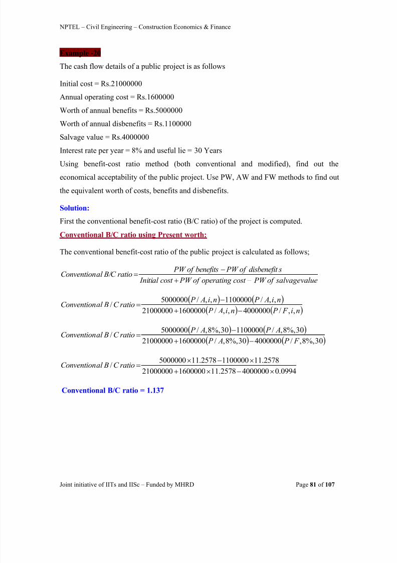
8/15/2019 2 Comparision of Alternatives
http://slidepdf.com/reader/full/2-comparision-of-alternatives 81/107
NPTEL – Civil Engineering – Construction Economics & Finance
Joint initiative of IITs and IISc – Funded by MHRD Page 81 of 107
Example -20
The cash flow details of a public project is as follows
Initial cost = Rs.21000000
Annual operating cost = Rs.1600000Worth of annual benefits = Rs.5000000
Worth of annual disbenefits = Rs.1100000
Salvage value = Rs.4000000
Interest rate per year = 8% and useful lie = 30 Years
Using benefit-cost ratio method (both conventional and modified), find out the
economical acceptability of the public project. Use PW, AW and FW methods to find out
the equivalent worth of costs, benefits and disbenefits.
Solution:
First the conventional benefit-cost ratio (B/C ratio) of the project is computed.
Conventional B/C ratio using Present worth:
The conventional benefit-cost ratio of the public project is calculated as follows;
value salvageof PW cost operating of PW cost Initial sdisbenefit of PW benefitsof PW
ratio B/C al Convention
ni F P ni A P
ni A P ni A P ratioC Bal Convention
,,/4000000,,/160000021000000,,/1100000,,/5000000
/
30%,8,/400000030%,8,/160000021000000
30%,8,/110000030%,8,/5000000/
F P A P A P A P
ratioC Bal Convention
0994.040000002578.111600000210000002578.1111000002578.115000000
/ ratioC Bal Convention
Conventional B/C ratio = 1.137

8/15/2019 2 Comparision of Alternatives
http://slidepdf.com/reader/full/2-comparision-of-alternatives 82/107
NPTEL – Civil Engineering – Construction Economics & Finance
Joint initiative of IITs and IISc – Funded by MHRD Page 82 of 107
Conventional B/C ratio using Annual worth:
value salvageof AW cost operating of W Acost initial of AW sdisbenefit of W Abenefitsof AW
ratio B/C al Convention
ni F Ani P AratioC Bal Convention
,,/40000001600000,,/2100000011000005000000
/
30%,8,/4000000160000030%,8,/2100000011000005000000
/ F A P A
ratioC Bal Convention
0088.0400000016000000888.02100000011000005000000
/ ratioC Bal Convention
Conventional B/C ratio = 1.137
Conventional B/C ratio using Future worth:
valuealvageS cost operating of W F cost initial of FW sdisbenefit of W F benefitsof FW
ratio B/C al Convention
4000000,,/1600000,,/21000000
,,/1100000,,/5000000/
ni A F ni P F ni A F ni A F
ratioC Bal Convention
400000030%,8,/160000030%,8,/2100000030%,8,/110000030%,8,/5000000/
A F P F A F A F ratioC Bal Convention
40000002832.11316000000627.10210000002832.11311000002832.1135000000
/ ratioC Bal Convention
Conventional B/C ratio = 1.137
As calculated above, the conventional benefit-cost ratio is found to be same by using any
of the equivalent worth methods i.e. PW method, AW method or FW method. As the
benefit-cost ratio of the public project is 1.137 (i.e. greater than 1.0), the project is
acceptable.

8/15/2019 2 Comparision of Alternatives
http://slidepdf.com/reader/full/2-comparision-of-alternatives 83/107
NPTEL – Civil Engineering – Construction Economics & Finance
Joint initiative of IITs and IISc – Funded by MHRD Page 83 of 107
Now the modified benefit-cost ratio (B/C ratio) of the project is calculated.
Modified B/C ratio using Present worth:
The modified benefit-cost ratio of the public project is calculated as follows;
value salvageof PW cost Initial cost operating of PW sdisbenefit of PW benefitsof PW ratio B/C Modified
n ,i , F / P
n ,i , A / P n ,i , A / P n ,i , A / P ratioC / B Modified
400000021000000160000011000005000000
308400000021000000
308160000030811000003085000000%, , F / P
%, , A / P %, , A / P %, , A / P ratioC / B Modified
0994.04000000210000002578.1116000002578.1111000002578.115000000
ratioC/BModified
Modified B/C ratio = 1.257
Modified B/C ratio using Annual worth:
value salvageof AW cost initial of AW cost operating of AW sdisbenefit of AW benefitsof AW
ratio B/C Modified
n,i,F/A4000000n,i,P/A21000000160000011000005000000ratioC/BModified
308400000030821000000160000011000005000000
%, , F / A%, , P / AratioC / B Modified
0088040000000888021000000160000011000005000000
..ratioC / B Modified
Conventional B/C ratio = 1.257
Modified B/C ratio using Future worth:
valuealvageS cost initial of FW cost operating of W F sdisbenefit of W F benefitsof FW
ratio B/C Modified

8/15/2019 2 Comparision of Alternatives
http://slidepdf.com/reader/full/2-comparision-of-alternatives 84/107
NPTEL – Civil Engineering – Construction Economics & Finance
Joint initiative of IITs and IISc – Funded by MHRD Page 84 of 107
400000021000000
160000011000005000000n ,i , P / F
n ,i , A / F n ,i , A / F n ,i , A / F ratioC / B Modified
400000030821000000
308160000030811000003085000000
%, , P / F
%, , A / F %, , A / F %, , A / F ratioC / B Modified
400000006271021000000283211316000002832113110000028321135000000
....
ratioC / B Modified
Modified B/C ratio = 1.257
The modified benefit-cost ratio of the public project is found to be 1.257.
As observed from above calculations, the B/C ratio of the project from both methods
(conventional and modified) is greater than 1.0, although the value is different. It may be
noted here that, although the magnitude of benefit-cost ratio differs between two methods
i.e. conventional B/C ratio and modified B/C ratio, but the decision to select or not a
project is not changed by use of any of the two methods.

8/15/2019 2 Comparision of Alternatives
http://slidepdf.com/reader/full/2-comparision-of-alternatives 85/107
NPTEL – Civil Engineering – Construction Economics & Finance
Joint initiative of IITs and IISc – Funded by MHRD Page 85 of 107
Lecture-14Incremental benefit-cost ratio analysis:-
The incremental benefit-cost ratio analysis is used to select the best alternative from a set
of mutually exclusive alternatives. Similar to incremental rate of return analysis, in thismethod also the incremental cash flow between the alternatives i.e. the differences in
benefits and costs between the alternatives are calculated and then the ratio of the
equivalent worth of incremental benefits to that of incremental costs is found out. In this
method, the alternative with large cost is selected, if the incremental benefits justify the
extra cost associated with it. In other words if the incremental B/C ratio is greater than or
equal to 1.0, then the larger cost alternative is selected. If incremental B/C ratio is less
than 1.0, then lower cost alternative is selected. While comparing the mutually exclusive
alternatives, the alternative with maximum B/C ratio (on its total cash flow) should not be
selected as the best alternative at first instance because the maximization of B/C ratio
may not guarantee that, best alternative is selected. However after carrying out the
incremental B/C ratio analysis, the selection of the best alternative may match with the
alternative with maximum B/C ratio on its total cash flow.
The incremental benefit-cost ratio analysis for comparison of mutually exclusive
alternatives is carried out in the following steps;
i) First, all the alternatives are arranged in increasing order of equivalent worth of costs.
The equivalent worth of cost of alternatives may be determined either by present
worth method, annual worth method or future worth method.
ii) The alternative with lowest equivalent cost is now compared with do-nothing
alternative (initial base alternative). In other words the B/C ratio of lowest equivalent
cost alternative on its total cash flow is calculated. If calculated B/C ratio is greater
than or equal to 1.0, then the lowest equivalent cost alternative becomes the new base
alternative. On the other hand if B/C ratio is less than 1.0, then this alternative is
removed from further analysis and the acceptability of the next higher equivalent cost
alternative as base alternative is found in the same manner as that was carried out for
the alternative with lowest equivalent cost. This process is continued till the base
alternative (acceptable alternative for which B/C ratio is greater than or equal to 1.0) is

8/15/2019 2 Comparision of Alternatives
http://slidepdf.com/reader/full/2-comparision-of-alternatives 86/107
NPTEL – Civil Engineering – Construction Economics & Finance
Joint initiative of IITs and IISc – Funded by MHRD Page 86 of 107
obtained. If no alternative is obtained in this manner, then do-nothing alternative is
selected i.e. none of the alternatives are selected, if this is an option.
iii) Now the incremental benefit, B and incremental cost, C (i.e. difference in benefits
and costs) between next higher equivalent cost alternative and the base alternative are
calculated and then incremental B/C ratio ( B/ C) i.e. ratio of the equivalent worth of
incremental benefits to that of incremental costs is obtained. If the incremental B/C
ratio ( B/ C) is greater than or equal to 1.0, then the base alternative is removed from
further analysis and the next higher equivalent cost alternative becomes the new base
alternative. On the other hand if B/ C is less than 1.0, then the higher equivalent
cost alternative is eliminated form further analysis and base alternative remains the as
the base. Then the incremental B/C ratio is calculated between the next higherequivalent cost alternative and the base alternative. This process is continued till the
last alternative is compared and in this way the best alternative is selected which
justifies the extra cost associated with it from the incremental benefits.

8/15/2019 2 Comparision of Alternatives
http://slidepdf.com/reader/full/2-comparision-of-alternatives 87/107
NPTEL – Civil Engineering – Construction Economics & Finance
Joint initiative of IITs and IISc – Funded by MHRD Page 87 of 107
The incremental B/C ratio analysis is illustrated in the following example.
Example -21
There are four mutually exclusive alternatives for a public project. Select the best
alternative using incremental B/C ratio analysis if interest rate is 7% per year. The cashflow details of the alternatives are shown in the following table. Each alternative has the
useful life of 40 years.Table 2.7 Cash flow of alternatives for the project
Alternative
Cash flow
Alternative-1
A1
Alternative-2
A2
Alternative-3
A3
Alternative-4
A4
Initial investment (Rs.)101000000 112000000 145200000 122800000
Annual operating andmaintenance cost (Rs.)
6700000 6450000 5780000 6135000
Worth of annual benefits (Rs.) 16420000 17200000 19100000 17900000
Useful life (Years) 40 40 40 40
Solution:
First the conventional B/C ratio will be used for the incremental benefit-cost analysis
for the comparison of above mutually exclusive alternatives. Present worth method will
be used for the calculation of equivalent worth of benefits and costs.
In order to arrange the alternatives in the increasing order of equivalent cost, first the
equivalent worth (present worth) of the costs of all the four alternatives are calculated.
Present worth of costs of Alternative-1 (A1):
n,i,A/P67000001010000001Aof tscosof PW
40%,7,A/P67000001010000001Aof tscosof PW
3317.1367000001010000001Aof tscosof PW
PW of costs of A1 = 190322390

8/15/2019 2 Comparision of Alternatives
http://slidepdf.com/reader/full/2-comparision-of-alternatives 88/107
NPTEL – Civil Engineering – Construction Economics & Finance
Joint initiative of IITs and IISc – Funded by MHRD Page 88 of 107
Present worth of costs of Alternative-2 (A2):
n,i,A/P64500001120000002Aof tscosof PW
40%,7,A/P64500001120000002Aof tscosof PW
3317.1364500001120000002Aof tscosof PW PW of costs of A2 = 197989465
Present worth of costs of Alternative-3 (A3):
n,i,A/P57800001452000003Aof tscosof PW
40%,7,A/P57800001452000003Aof tscosof PW
3317.1357800001452000003Aof tscosof PW
PW of costs of A3 = 222257226
Present worth of costs of Alternative-4 (A4):
n ,i , A / P Aof tscosof PW 61350001228000004
40761350001228000004 %, , A / P Aof tscosof PW
33171361350001228000004 . Aof tscosof PW
PW of costs of A4 = 204589980
As observed from the above calculations, the order of alternatives from lowest equivalent
cost to highest equivalent cost is A1, A2, A4 and A3.
The lowest equivalent cost alternative A1 is first compared against do-nothing alternative
i.e. the B/C ratio of alternative A1 on its cash flow is calculated.
cost emaintenancand operating of PW investment Initial benefitsof PW
A1of ratio B/C
40%,7,A/P6700000101000000
40%,7,A/P164200001Aof ratioC/B
3317.1367000001010000003317.1316420000
1Aof ratioC/B
B/C ratio of alternative A1 = 1.150
As the B/C ratio of alternative A1 is greater than 1.0, A1 now becomes the base
alternative and is compared against the next higher equivalent cost alternative i.e.

8/15/2019 2 Comparision of Alternatives
http://slidepdf.com/reader/full/2-comparision-of-alternatives 89/107
NPTEL – Civil Engineering – Construction Economics & Finance
Joint initiative of IITs and IISc – Funded by MHRD Page 89 of 107
alternative A2. Now the incremental benefits and incremental costs between A2 and A1
are calculated and the incremental B/C ratio is obtained.
78000016420000-17200000A1)andA2(between benefitsannuallIncrementa
1039872613.3317780000407%,P/A,780000 benefitsannuallincrementaof (PW)rthPresent wo
PW of incremental benefits (between A2 and A1) = Rs.10398726
11000000101000000-112000000A1)andA2(betweeninvestmentinitiallIncrementa
250000-6700000-6450000
A1)andA2(betweencostemaintenancandoperatingannuallIncrementa
766707513.331725000011000000
407%,P/A,250000-11000000costslincrementaof (PW)rthPresent wo
PW of incremental costs (between A2 and A1) = Rs.7667075
Incremental B/C ratio (between alternative A2 and A1) = 1.356
The incremental B/C ratio between alternatives A2 and A1 can also be calculated by
finding out the ratio of the differences in present worth of benefits of alternatives to that
of costs. This calculation is shown below.
21890651433171316420000
407%,P/A,16420000A1ealternativof benefitsof PW
.
1903223903317136700000101000000
407%,P/A,6700000101000000A1ealternativof costsof PW
.
22930524033171317200000
407%,P/A,17200000A2ealternativof benefitsof PW
.
1979894653317.136450000101000000
407%,P/A,6450000112000000A2ealternativof costsof PW
35617667075
10398726costslincrementaof PW
benefitslincrementaof PWΔC
ΔB ratioB/ClIncrementa .

8/15/2019 2 Comparision of Alternatives
http://slidepdf.com/reader/full/2-comparision-of-alternatives 90/107
NPTEL – Civil Engineering – Construction Economics & Finance
Joint initiative of IITs and IISc – Funded by MHRD Page 90 of 107
Thus same incremental B/C ratio is obtained.As the incremental B/C ratio is greater than 1.0, alternative A2 becomes the new base
alternative and alternative A1 is removed from further analysis. Alternative A2 is now
compared against the next higher equivalent cost alternative i.e. alternative A4. The
incremental B/C ratio between alternatives A4 and A2 is determined in the same manner
as that was determined between alternatives A2 and A1.
Now the entire calculation for selecting the best alternative using incremental B/C ratio
analysis is presented in Table 2.8.
Table 2.8 Comparison of alternatives using incremental B/C ratio* analysis
Comparison of Alternatives
Cash flow
Between A1and do-nothingalternative
BetweenA2 and A1
BetweenA4 and A2
BetweenA3 and A4
Incremental initial investment (Rs.) 101000000 11000000 10800000 22400000
Incremental annual operating andmaintenance cost (Rs.) 6700000 -250000 -315000 -355000
Incremental annual benefit (Rs.) 16420000 780000 700000 1200000
PW of incremental benefit (Rs.) 218906514 10398726 9332190 15998040
PW of incremental cost (Rs.) 190322390 7667075 6600515 17667247
Incremental B/ C Ratio 1.150 1.356 1.414 0.906
Increment justified Yes Yes Yes No
* Conventional B/C ratio
The comparison of above alternatives using incremental B/C ratio analysis as shown in
Table 2.8 is briefly presented below.
The lowest equivalent cost alternative A 1 is compared against the do-nothing
alternative (initial base alternative). In other words B/C ratio of alternative A 1 on
356.1190322390-197989465218906514-229305240
A1andA2 betweentscosof PWinDifferenceA1andA2 between benefitsof PWinDifference
ΔC
ΔB A1)andA2(betweenratioB/ClIncrementa

8/15/2019 2 Comparision of Alternatives
http://slidepdf.com/reader/full/2-comparision-of-alternatives 91/107
NPTEL – Civil Engineering – Construction Economics & Finance
Joint initiative of IITs and IISc – Funded by MHRD Page 91 of 107
its total cash flow is calculated. The obtained B/C ratio is 1.150 which is greater
than 1.0. Thus alternative A1 now becomes the new base alternative.
Now alternative A1 is compared against the next higher equivalent cost
alternative i.e. A2 . The incremental B/C ratio between alternatives A2 and A1 is
calculated. The calculated incremental B/C ratio is 1.356 which is greater than
1.0. Thus alternative A2 now becomes the base alternative and alternative A1 is
eliminated from further analysis.
Alternative A2 is now compared against the next higher equivalent cost
alternative i.e. alternative A4 . The calculated incremental B/C ratio between
alternatives A4 and A2 is 1.414 (greater than 1.0). Alternative A4 now becomes
the base alternative and alternative A2 is eliminated.
Alternative A4 is now compared against the next higher equivalent cost
alternative i.e. alternative A3 (last alternative). The incremental B/C ratio between
alternatives A3 and A4 is 0.906 which is less than 1.0. Thus the incremental cost
associated with alternative A3 is not justified. Hence alternative A4 is selected
as the best alternative as no other alternative is left for comparison . In other
words alternative A4 is the highest equivalent cost alternative which is associated
with the last justified increment i.e. incremental B/C ratio greater than 1.0.
It may be noted here that the B/C ratios of the alternatives on their individual cash flowscould have been calculated at the beginning of the analysis to eliminate any alternative(s)
that has a B/C ratio less than 1.0 and that alternative(s) need not be considered further in
the incremental benefit-cost ratio analysis. However this step is not necessary because the
alternative with B/C ratio less than 1.0 on its cash flow will eliminated in the process of
incremental analysis. In this example the values of B/C ratio of the alternatives A1, A2,
A3 and A4 on their individual cash flows are 1.150, 1.158, 1.146 and 1.166 respectively
(all greater than 1.0). The calculation of B/C ratio is shown only for alternative A1. The
B/C ratio of other alternatives can be similarly calculated.
The above incremental B/C ratio analysis was carried out using conventional B/C ratio.
The same analysis can also be carried out by using modified B/C ratio. As already stated,
in modified B/C ratio, the operating and maintenance cost is subtracted from the benefits

8/15/2019 2 Comparision of Alternatives
http://slidepdf.com/reader/full/2-comparision-of-alternatives 92/107
NPTEL – Civil Engineering – Construction Economics & Finance
Joint initiative of IITs and IISc – Funded by MHRD Page 92 of 107
in the numerator. The incremental B/C ratio analysis using modified B/C ratio for the
comparison of above mutually exclusive alternatives is describe below.
The order of alternatives from lowest to highest equivalent cost (present worth of cost)
will depend only on the initial investment as the annual operating and maintenance cost(considered similar to disbenefits) is subtracted from the benefits in the numerator of
modified B/C ratio. Thus the order of alternatives from lowest to highest equivalent cost
(i.e. initial investment) is A1, A2, A4 and A3 (same as earlier). Now the incremental
benefit-cost analysis using modified B/C ratio is carried out in the same manner as that
was done using conventional B/C ratio and is presented in Table 2.9.
Table 2.9 Comparison of alternatives using incremental B/C ratio** analysis
Comparison of Alternatives
Cash flow
Between A1and do-nothingalternative
BetweenA2 and A1
BetweenA4 and A2
BetweenA3 and A4
Incremental initial investment (Rs.) 101000000 11000000 10800000 22400000
Incremental net annual benefit *** (Rs.) 9720000 1030000 1015000 1555000
PW of incremental net benefit (Rs.) 129584124 13731651 13531676 20730794
PW of incremental cost i.e. incrementalinitial investment (Rs.) 101000000 11000000 10800000 22400000
Incremental B/ C Ratio 1.283 1.248 1.253 0.925
Increment justified Yes Yes Yes No
** Modified B/C ratio
*** Net annual benefit for an alternative is obtained by subtracting the annual operating
and maintenance cost from its annual benefits. Incremental net annual benefit is thedifference in net annual benefits between two alternatives. Considering the comparison
between alternatives A4 and A2, the calculation of incremental net annual benefit is
shown below.

8/15/2019 2 Comparision of Alternatives
http://slidepdf.com/reader/full/2-comparision-of-alternatives 93/107
NPTEL – Civil Engineering – Construction Economics & Finance
Joint initiative of IITs and IISc – Funded by MHRD Page 93 of 107
107500006450000-17200000
costemaintenancandoperatingannual- benefitsannualA2ealternativof benefitannualnetThe
117650006135000-17900000
costemaintenancandoperatingannual- benefitsannualA4ealternativof benefitannualnetThe
101500010750000-11765000A2andA4esalternativ between benefitannualnetlincrementaThe
Thus the incremental net annual benefit between two alternatives A4 and A2 is
Rs.1015000, which is shown in Table 2.9.
From Table 2.9, it is observed that the best alternative is A4 , which is same as the
outcome obtained from incremental B/C ratio analysis using the conventional B/C ratio.
In other words the same outcome regarding the best alternative is obtained, however the
values of B/C ratios obtained were different. Similar to present worth, the incremental
B/C ratio analysis can also be carried out by calculating the annual worth (AW) or futureworth (FW) of benefits and costs of alternatives.

8/15/2019 2 Comparision of Alternatives
http://slidepdf.com/reader/full/2-comparision-of-alternatives 94/107
NPTEL – Civil Engineering – Construction Economics & Finance
Joint initiative of IITs and IISc – Funded by MHRD Page 94 of 107
Lecture-15Breakeven analysis:-
The breakeven analysis is used to calculate the value of a factor (or variable) at which the
expenditures and revenues of a project or alternative are equal. This value of the variable
is known as the breakeven point. Corresponding to the breakeven point, profit or loss can
be determined if the expected value of the variable is higher or lower than the breakeven
value. In this regard the breakeven point governs the economic acceptability of the
project or the alternative. The breakeven analysis is also used for comparing two
alternatives by determining the breakeven point i.e. the quantity of a factor (common to
both the alternatives) at which the total equivalent worth of both alternatives are equal.
The examples of some of the factors which are used in the breakeven analysis are
quantities produced per year, hours of operation per year, rate of return per year and
useful life etc. and the breakeven value of these factors are calculated to find out the
economical acceptability of a single alternative or to select the best one between the
alternatives. The breakeven point between expenditure and revenue for a single
alternative is shown in Fig. 2.32. Here „x is the factor that mainly affects the expenditure
and revenue of the alternative.
Fig. 2.32 Schematic diagram for breakeven point of a single alternative
In Fig. 2.32, the equivalent worth of expenditure and revenue are plotted as functions of
the quantity of factor „x . The breakeven point corresponds to that value of the factor „x
Breakeven point
Quantity of ‘x’
Equivalentworth (Rs.)
Revenue
Expenditure
Breakeven

8/15/2019 2 Comparision of Alternatives
http://slidepdf.com/reader/full/2-comparision-of-alternatives 95/107
NPTEL – Civil Engineering – Construction Economics & Finance
Joint initiative of IITs and IISc – Funded by MHRD Page 95 of 107
at which the equivalent worth of expenditure and revenue of the alternative are equal i.e.
the relationships representing the expenditure and revenue as functions of „x intersect
each other (shown in Fig. 2.32).
The breakeven point between two alternatives is shown in Fig. 2.33.
Fig. 2.33 Schematic diagram of breakeven point between two alternatives
In this figure the total equivalent worth i.e. equivalent worth of net cash flow (i.e.
expenditures and revenues) of the alternatives are plotted at various values of the
common factor „x . The intersection of the total equivalent worth of two alternatives
gives the breakeven point i.e. the value of the common factor „x at which the values of
total equivalent worth of the two alternatives are equal. If the expected value of „x is less
than the breakeven value, Alternative-1 is selected as its total equivalent worth (assuming
it as negative cash flow i.e. cost greater than revenue) is less than that of Alternative-2 as
evident from Fig. 2.33. Similarly when the expected value of „x is greater than the
breakeven value, Alternative-2 is selected as it shows lower equivalent worth (i.e. lowercost) compared to Alternative-1. In Fig. 2.32 the variations of equivalent worth of
expenditure and revenue of the single alternative and in Fig. 2.33 the variations of total
equivalent worth of two alternatives are considered as linear functions of the value of
factor „x . Sometimes these relationships may also be non-linear. In the breakeven
Quantity of ‘x’
Total equivalentworth (Rs.)
Alternative-1
Alternative-2
Breakeven
Breakeven point

8/15/2019 2 Comparision of Alternatives
http://slidepdf.com/reader/full/2-comparision-of-alternatives 96/107
NPTEL – Civil Engineering – Construction Economics & Finance
Joint initiative of IITs and IISc – Funded by MHRD Page 96 of 107
analysis, the equivalent worth of expenditures and revenues can be calculated either by
present worth method, future worth method or annual worth method by taking into
account the time value of money. The annual worth method is normally used when the
quantities of the variable (on which the expenditures and the revenues mostly depend) are
expressed on annual basis.
The following example will illustrate the breakeven analysis for a single alternative.
Example -22
A concrete mixer has the following cash flow details;
Initial purchase price = Rs.750000,
Annual operating and maintenance cost = Rs.45000
Salvage value = Rs.210000,Useful life = 10 years
In addition one operator is required to operate the concrete mixer at cost of Rs.30 per
hour. The production (preparation) rate of concrete of the mixer is 0.1m 3 per hour. The
revenue to be generated from production of 1m 3 of concrete is Rs.1000. The interest rate
is 11% per year. How many „m 3 of concrete need to be produced per year so that the
revenue generated breakevens with the expenditure?
Solution:In order to find out the breakeven value of the concrete volume (in „m 3 ) per year, the
equivalent uniform annual worth of expenditure will be equated to that of revenue.
Let „x m 3 is the volume of concrete produced by the concrete mixer per year.
The operator cost is Rs.30 per hour.
The operator cost (Rs.) per year is given by;
x300.Rsyear
mxm1.0
hour 1hour 1
30.Rs 3
3
Now the equivalent uniform annual worth (Rs.) of expenditure is given by;
x30045000n,i,P/A750000AW e
x3004500010%,11,P/A750000AW e
x300172350x300450001698.0750000AW e

8/15/2019 2 Comparision of Alternatives
http://slidepdf.com/reader/full/2-comparision-of-alternatives 97/107
NPTEL – Civil Engineering – Construction Economics & Finance
Joint initiative of IITs and IISc – Funded by MHRD Page 97 of 107
The equivalent uniform annual worth (Rs.) of revenue is calculated as follows;
x1000n,i,F/A210000AW r
x100010%,11,F/A210000AW r
x100012558x10000598.0210000AW r Now equating equivalent uniform annual worth of expenditure with that of revenue;
r e AWAW
x100012558x300172350
3m274.228x
Thus the volume of concrete to be produced by the concrete mixer per year i.e. the
breakeven quantity at which the expenditure incurred is equal to the revenue generated is
228.274 m 3. If the volume of concrete produced per year is different from the breakeven
value, then there will change in the net cash flow as shown below;
If x is equal to 200 m 3 (i.e. less than breakeven value), the equivalent uniform annual
worth of expenditure and revenue are given by;
Expenditure
x3004500010%,11,P/A750000AW e
232350.Rs200300450001698.0750000AW e
Revenue
x100010%,11,F/A210000AW r
212558.Rs20010000598.0210000AW r
AW e > AW r
If x is equal to 250 m 3 (i.e. greater than breakeven value), the equivalent uniform annual
worth of expenditure and revenue are given by;
Expenditure
x3004500010%,11,P/A750000AW e
247350.Rs250300450001698.0750000AW e
Revenue
x100010%,11,F/A210000AW r
262558.Rs25010000598.0210000AW r

8/15/2019 2 Comparision of Alternatives
http://slidepdf.com/reader/full/2-comparision-of-alternatives 98/107
NPTEL – Civil Engineering – Construction Economics & Finance
Joint initiative of IITs and IISc – Funded by MHRD Page 98 of 107
AW r > AW e
Thus from above calculations it is observed that, equivalent annual worth of revenue is
less than that of expenditure, when the volume of concrete produced per year is less than
the breakeven value and on the other hand, equivalent annual worth of revenue is more
than that of expenditure, when the volume of concrete produced per year is greater than
the breakeven value.
The breakeven point is also graphically shown in Fig. 2.34.
Fig. 2.34 Equivalent uniform annual worth of expenditure and revenue
and breakeven point
The equivalent uniform annual worth of expenditure and revenue are calculated at
different values of volume of concrete produced per year using the respective expressions
as mentioned earlier and are shown in the above figure.
The breakeven point can also be calculated by equating the equivalent present worth of
expenditures to that of revenues as shown below.
Present worth of expenditure:
n,i,A/Px300n,i,A/P45000750000PW e
10%,11,A/Px30010%,11,A/P45000750000PW e
0
50000
100000
150000
200000
250000
300000
350000
400000
450000
0 50 100 150 200 250 300 350 400 450
Volume of concrete (m 3)
E q u
i v a
l e n
t u n
i f o r m
a n n u a l w
o r t h
( R s . )
Expenditure
Revenue
Breakeven value

8/15/2019 2 Comparision of Alternatives
http://slidepdf.com/reader/full/2-comparision-of-alternatives 99/107
NPTEL – Civil Engineering – Construction Economics & Finance
Joint initiative of IITs and IISc – Funded by MHRD Page 99 of 107
x76.17661015014x3008892.58892.545000750000PW e
Present worth of revenue:
n,i,A/Px1000n,i,F/P210000PW r
10%,11,A/Px100010%,11,F/P210000PW r
x2.588973962x10008892.53522.0210000PW r
Now equating equivalent present worth of expenditure with that of revenue;
r e PWPW
x2.588973962x76.17661015014
3m275.228x
Thus the breakeven value of volume of concrete to be produced by the concrete mixer per
year is 228.275 m 3 which is same as the value obtained by annual worth method stated
earlier.

8/15/2019 2 Comparision of Alternatives
http://slidepdf.com/reader/full/2-comparision-of-alternatives 100/107
NPTEL – Civil Engineering – Construction Economics & Finance
Joint initiative of IITs and IISc – Funded by MHRD Page 100 of 107
Lecture-16
Breakeven analysis for two and more than two alternatives:-
Br eakeven anal ysis between two al ternatives
The breakeven analysis between two alternatives is carried out by equating the equivalent
worth of cash flows of both the alternatives. For determining the breakeven point
between the alternatives, a factor or variable (as required) must be common to both the
alternatives and the corresponding cost or revenue element is expressed in terms of this
common variable. As already stated, the total equivalent worth of alternatives can be
calculated either by present worth method, future worth method or annual worth method
by considering the time value of money. The breakeven analysis between two alternatives
is presented in the following example.
Example -23
A construction company has two alternatives to purchase an excavator which is to be
employed at a construction site for excavation of earth. The cash flow details of the two
alternatives are presented as follows;
Alternative-1: Initial purchase cost = Rs.4865000
Salvage value = Rs.1250000
Useful life = 12 years
Operating cost:
The operating cost for excavating 1m 3 of earth is Rs.11.0. The excavator (Alternative-1)
can excavate 52 m 3 of earth in one hour.
Alternative-2: Initial purchase cost = Rs.5350000
Salvage value = Rs.1410000
Useful life = 12 years
Operating cost:
The operating cost for excavating 1m 3 of earth is Rs.8.0. The excavator (Alternative-2)
can excavate 60 m 3 of earth in one hour.

8/15/2019 2 Comparision of Alternatives
http://slidepdf.com/reader/full/2-comparision-of-alternatives 101/107
NPTEL – Civil Engineering – Construction Economics & Finance
Joint initiative of IITs and IISc – Funded by MHRD Page 101 of 107
The c ompany s minimum attractive rate of return (MARR) is 10.5% per year. How many
hours the excavators have to operate per year, for the equivalent uniform annual worth of
cash flows of both the alternatives to be equal?
Solution:Let „y is the number of operating hours per year.
The annual operating cost (Rs.) for Alternative-1 is given by;
y572.Rsyear hour y
hour 1m52
m111.Rs 3
3
Now the equivalent uniform annual worth (Rs.) of Alternative-1 is given by;
n,i,F/A1250000y572n,i,P/A4865000AW 1
12%,5.10,F/A1250000y57212%,5.10,P/A4865000AW 1 y5726749460454.01250000y5721504.04865000AW 1
The annual operating cost (Rs.) for Alternative-2 is given by;
y480.Rsyear hour y
hour 1m60
m18.Rs 3
3
The equivalent uniform annual worth (Rs.) of Alternative-2 is given by;
n,i,F/A141000y480n,i,P/A5350000AW 2
12%,5.10,F/A1410000y48012%,5.10,P/A5350000AW 2
y4807406260454.01410000y4801504.05350000AW 2
Now equating equivalent uniform annual worth Alternative-1 to that of Alternative-2;
21 AWAW
y480740626y572674946
hours9.713y
Thus the breakeven value of number of operating hours per year is 713.9 hours, at which
the equivalent uniform annual worth of Alternative-1 is equal to that of Alternative-2.
The breakeven point is also shown in Fig. 2.35. The equivalent uniform annual worth of
both the alternatives are determined at different values of annual operating hours and are
shown in Fig. 2.35.

8/15/2019 2 Comparision of Alternatives
http://slidepdf.com/reader/full/2-comparision-of-alternatives 102/107
NPTEL – Civil Engineering – Construction Economics & Finance
Joint initiative of IITs and IISc – Funded by MHRD Page 102 of 107
Fig. 2.35 Equivalent uniform annual worth and breakeven point between Alternative-1 and Alternative-2
The equivalent uniform annual worth of both the alternatives is negative as cash outflows
(i.e. expenditures) are greater than the cash inflows (i.e. revenues). Thus the equivalent
uniform annual worth of both the alternatives shown in Fig. 2.35 can also be stated as
equivalent uniform annual cost. The line representing the equivalent uniform annual cost
of Alternative-1 has greater slope than Alternative-2 as observed from this figure. In
other words Alternative-1 has higher annual variable cost (Rs.572y) as compared to
Alternative-2 (Rs.480y). Similarly Alternative-2 has higher constant equivalent annual
cost (Rs.740626) than Alternative-1 (Rs.674946), as observed from expressions of
equivalent uniform annual worth of both the alternatives and also from the above figure.
If the expected annual operating hours are less than the breakeven value (i.e. 713.9
hours), then the construction company should select Alternatives-1 as its equivalent
annual cost is less than that of Alternative-2 (as evident from Fig. 2.35). Similarly if the
expected annual operating hours are greater than breakeven value, then Alternative-2should be selected as it shows lower equivalent annual cost as compared to Alternative-1.
0
200000
400000
600000
800000
1000000
1200000
1400000
0 100 200 300 400 500 600 700 800 900 1000 1100 1200Annual operating period (Hours)
E q u
i v a l e n
t u
i n f o r m
a n n u a
l w o r t h
( R s . )
Alternative-1
Alternative-2
Breakeven point

8/15/2019 2 Comparision of Alternatives
http://slidepdf.com/reader/full/2-comparision-of-alternatives 103/107
NPTEL – Civil Engineering – Construction Economics & Finance
Joint initiative of IITs and IISc – Funded by MHRD Page 103 of 107
Br eakeven an alysis for more than two alternati ves
The breakeven analysis can also be carried out for more than two alternatives. Similar to
the case of two alternatives, the required factor or variable must be common to all the
alternatives. In this analysis the pair-wise comparison between the alternatives is carried
out to determine the corresponding breakeven point. The schematic diagram of breakeven
analysis between three alternatives ( A1 , A2 and A3 ) is shown in Fig. 2.36. In this figure
the lines represent the total equivalent worth (i.e. equivalent worth of net cash flow) of
the alternatives at different values of the common variable „x .
Fig. 2.36 Schematic diagram of breakeven points for three alternatives
In this figure the total equivalent worth is assumed as the equivalent annual cost of the
alternatives. Further „x1 , „x2 and „x3 represent the breakeven points between
alternatives A1 and A3 , between A2 and A3 and between A1 and A2 respectively. As
already mentioned, the breakeven points „x1 , „ x2 and „ x3 can be calculated by equating
the equivalent worth of the corresponding pair of the alternatives. If the expected or
estimated value of common variable „ x is less than „ x1 (i.e. the breakeven value between
A1 and A3), then alternative A3 is selected as it shows lowest equivalent annual cost as
Total equivalentworth (Rs.)
Quantity of common variable ‘x’
A3
A1
A2
x3x1
x2

8/15/2019 2 Comparision of Alternatives
http://slidepdf.com/reader/full/2-comparision-of-alternatives 104/107
NPTEL – Civil Engineering – Construction Economics & Finance
Joint initiative of IITs and IISc – Funded by MHRD Page 104 of 107
evident from Fig. 2.36. Similarly if the expected value of common variable „ x lies in
between „x1 and „x3 , then alternative A1 is selected as its equivalent annual cost is
lowest within this range of the common variable. Further if the expected value of
common variable is greater than „ x3 , then alternative A2 is preferred over other
alternatives as it shows lowest equivalent annual cost as compared to other alternatives.
In this analysis, „x2 (the breakeven p oint between alternatives A2 and A3 ) lies between
the breakeven points „ x1 and „ x3 and alternative A1 has lowest equivalent annual cost
between breakeven points „ x1 and „ x2 and between „x2 and „ x3 (i.e. between „ x1 and
„x3 as already stated) .
The breakeven analysis between three alternatives is presented in the following example.
Example -24 (Using data of Example-23)
In this example, details about third alternative are mentioned along with the two
alternatives stated in Example-23 for carrying out breakeven analysis between three
alternatives.
A construction company has three alternatives to purchase an excavator which is to be
employed at a construction site for excavation of earth. The cash flow details of all the
three alternatives are presented as follows;
Alternative-1: Initial purchase cost = Rs.4865000
Salvage value = Rs.1250000
Useful life = 12 years
Operating cost:
The operating cost for excavating 1m 3 of earth is Rs.11.0. The excavator (Alternative-1)
can excavate 52 m 3 of earth in one hour.
Alternative-2: Initial purchase cost = Rs.5350000
Salvage value = Rs.1410000
Useful life = 12 yearsOperating cost:
The operating cost for excavating 1m 3 of earth is Rs.8.0. The excavator (Alternative-2)
can excavate 60 m 3 of earth in one hour.
Alternative-3: Initial purchase cost = Rs.5975000
Salvage value = Rs.1500000

8/15/2019 2 Comparision of Alternatives
http://slidepdf.com/reader/full/2-comparision-of-alternatives 105/107
NPTEL – Civil Engineering – Construction Economics & Finance
Joint initiative of IITs and IISc – Funded by MHRD Page 105 of 107
Useful life = 12 years
Operating cost:
The operating cost for excavating 1m 3 of earth is Rs.6.0. The excavator (Alternative-3)
can excavate 67 m 3 of earth in one hour.
The company s minimum attractive rate of return (MARR) is 10.5% per year. Determine
the economical alternative at different values of annual operating hours.
Solution:
In this case the pair-wise comparison between the alternatives is carried out to determine
the corresponding breakeven point.
Let „y is the number of operating hours per year.
As already determined in Example-23, the equivalent uniform annual worth of
Alternative-1 and Alternative-2 are as follows;
y572674946AW 1
y480740626AW 2
The annual operating cost (Rs.) for Alternative-3 is given by;
y402.Rsyear hour y
hour 1m67
m16.Rs 3
3
Now the equivalent uniform annual worth (Rs.) of Alternative-3 is given by;
n,i,F/A1500000y402n,i,P/A5975000AW 3
12%,5.10,F/A1500000y40212%,5.10,P/A5975000AW 3
y4028305400454.01500000y4021504.05975000AW 3
The equivalent uniform annual worth of all the alternatives can also be stated as
equivalent uniform annual cost, as it is negative. Now the equivalent uniform annual
worth of all the three alternatives are determined at different values of annual operating
hours and are shown in Fig. 2.37.

8/15/2019 2 Comparision of Alternatives
http://slidepdf.com/reader/full/2-comparision-of-alternatives 106/107
NPTEL – Civil Engineering – Construction Economics & Finance
Joint initiative of IITs and IISc – Funded by MHRD Page 106 of 107
Fig. 2.37 Equivalent uniform annual worth and breakeven points between the alternatives
From this figure, it is observed that there are three breakeven points i.e. P 1 between
Alternative-1 and Alternative-2, P 2 between Alternative-1 and Alternative-3 and P 3
between Alternative-2 and Alternative-3. The breakeven points are determined by
equating the equivalent uniform annual worth of the corresponding alternatives.
For breakeven point P 1, equating the equivalent uniform annual worth Alternative-1 to
that of Alternative-2;
21 AWAW
674946 572 740626 480 y y
hours9.713y
For breakeven point P 2, equating the equivalent uniform annual worth Alternative-1 to
that of Alternative-3;
31 AWAW
674946 572y 830540 402y
hours915.3y
For breakeven point P 3, equating the equivalent uniform annual worth Alternative-2 to
that of Alternative-3;
32 AWAW
0
200000
400000
600000
800000
1000000
1200000
1400000
1600000
0 200 400 600 800 1000 1200 1400 1600 1800
Annual operating period (Hours)
E q u
i v a
l e n
t u n
i f o r m
a n n u a l w o r t h
( R s . )
Alternative-1
Alternative-2
Alternative-3
P 1P 3
P 2
8/15/2019 2 Comparision of Alternatives
http://slidepdf.com/reader/full/2-comparision-of-alternatives 107/107
NPTEL – Civil Engineering – Construction Economics & Finance
740626 480y 830540 402y
hours7.1152y
If the expected annual operating hours are less than the 713.9 hours (breakeven point P 1),
then the construction company should select Alternatives-1 as it shows lowest equivalentannual cost as compared to other alternatives as observed from Fig. 2.37. Similarly
Alternative-2 should be selected, if the expected annual operating hours lie between
713.9 and 1152.7 hours (between breakeven points P 1 and P 3) as its equivalent annual
cost is lowest than other alternatives. Further, Alternative-3 should be selected, if the
expected annual operating hours are greater than 1152.7 hours (breakeven point P 3), as it
shows lowest equivalent annual cost as compared to other alternatives as evident from
Fig. 2.37.
It is to be noted here that, similar to Example-1 (Lecture-2 of this module), commas at
appropriate places for the numbers can be placed in other examples presented in different
lectures.
Related Documents