1opus.bath.ac.uk/37762/1/Remanufacturing_13_09_13.doc · Web viewPRODUCT AND SALES CONTRACT DESIGN IN REMANUFACTURING We develop and analyze an economic model of remanufacturing to

PRODUCT AND SALES CONTRACT DESIGN IN REMANUFACTURING

We develop and analyze an economic model of remanufacturing to address two main research

questions. First, we explore which market, cost, and product type conditions induce a profit-

maximizing firm to be a remanufacturer, given a separate (secondary) remanufactured goods

market. Such markets exist for consumer goods, where “newness” is a differentiating factor.

Second, we describe what effect profitable remanufacturing has on the environment. Our stylized

modeling framework for analyzing these issues incorporates three components: lease contracting,

product design, and remanufacturing volume. To operationalize this framework, we model and

solve for the optimal decisions of two firm types: a non-remanufacturer, which we call a

traditional firm, and a remanufacturer, which we call a green firm. We describe conditions under

which remanufacturing is (and is not) profitable, and demonstrate that under certain cost and

market conditions remanufacturing has negative consequences for the environment. Our results

have implications for firms and policy makers who would like to choose remanufacturing as a

strategy to improve profitability and environmental performance, given the existence of

conditions under which neither might occur.

Keywords: product design; remanufacturing; green consumerism; durable goods; economic

modeling

i

1. INTRODUCTION AND LITERATURE REVIEW

Among other benefits, remanufacturing delivers value to new markets because items that consumers use

in one market can be collected, reworked, tested, and reinstalled for resale in another market to a different

group of consumers. Consider, for example, that commercial refrigerators from Europe are

remanufactured and then resold in Ghana (Refrigerator Energy Efficiency Project 2013), older generation

wind turbines are remanufactured and then resold to serve small communities in Africa (London

Environmental Investment Forum 2012), and after-use medical imaging devices are remanufactured and

then resold to veterinary practices and hospitals around the world (Centre for Remanufacturing and Reuse

2008). In a similar vein, perhaps most notably as a prototype illustration, post-contract mobile phones

produced in the USA are remanufactured and then resold in Brazil (Skerlos et al 2006). Several factors

enhance the profitability of such mobile phone remanufacturing operations. First, the access to a

secondary market gives remanufacturers the benefit of a “second life” for their phones (European

Parliament 2003, Kharif 2002, Marcussen 2003). Second, improved product designs allowing for

refurbished “cores” lend themselves to efficient disassembly and testing, which in turn gives

remanufacturers the benefit of reduced remanufacturing costs (Lindholm 2003; Seliger et al 2003). Third,

the introduction of fixed-term consumer contracts gives remanufacturers the benefit of maintaining

ownership and managing the useful lives of their mobile phones effectively (Canning 2006; Coronado

Mondragon et al 2011).

Accordingly, in this paper, we develop a stylized analytical model of remanufacturing that

incorporates the interrelationships amongst these three factors to answer and analyze two key research

questions. As our first research question, we ask which market, cost, and product type conditions induce

a profit-maximizing firm to become a remanufacturer when a separate secondary market exists for the

firm’s remanufactured goods. As the above examples suggest, the existence of such a secondary market

often can be observed when product “newness” is a factor that separates a firm’s new-goods market from

its remanufactured-goods market such that there is no overlap or cannibalization between the two (see, for

example, Atasu et al. 2010 and Guide and Li 2010).

1

As the above examples also suggest, the processes linked to remanufacturing such as disassembly,

reassembly, and resale, have implications for decisions made earlier in the product life cycle, such as

product design and sales contracting. Indeed, Xerox not only changed its business model completely to

operate a leasing scheme that supports its remanufacturing operations by keeping ownership of the

product within the organization (Atasu et al 2010), but also revised its product design process to add

product requirements for easy disassembly and testing (Nasr and Thurston 2006). Therefore, in

investigating our first research question, we develop an analytical model of remanufacturing that

explicitly considers a firm’s sales contract and product design decisions in support of its remanufacturing

operations.

As our second research question, we ask how becoming a remanufacturer ultimately impacts the

environment. Conventional wisdom indicates that remanufacturing, as a general rule, tends to be less

harmful to the environment and is a benefit for society as a whole (Ferrer and Whybark 2000, Guide

2000). However, remanufacturing also can be attributed to negative environmental consequences due to

the disposal of product components that are not remanufactured. For example, the remanufacturing of

technology products (such as mobile phones) has been linked to adverse environmental effects in the far-

east (United Nations Environment Program, 2005). In such cases, as typically is the case for

remanufacturing in general, the products are disassembled and the components that are amenable to reuse

are extracted, but what remains then enters the waste stream. Therefore, in investigating our second

research question, we explicitly incorporate the net environmental effects of remanufacturing into our

model to assess the overall environmental impact of a profitable remanufacturer by accounting for the

volume of un-remanufactured components that end up in the waste stream. Ultimately, this

environmental damage can be directly linked to the product design decision of the firm as well as to the

quantity of available items that are remanufactured. The answer to our second research question therefore

has implications not only for firms interested in remanufacturing, but also for regulators interested in

inducing firms to become remanufacturers or in helping local economies through the promotion of

remanufacturing.

2

Our modeling framework for analyzing these questions incorporates three components, namely, lease

contracting, product design, and remanufacturing volume. We develop the construct of a lease contract,

which ensures predictable returns at regular time intervals (Robotis et al. 2012), to reflect the notion that

customer behavior is a determinant of remanufacturing effectiveness because that behavior determines

both the condition and the timing of returns. We include the notion of product design in our framework

because, as Bras and McIntosh (1999) and Debo et al. (2005) discuss, design decisions that support easier

disassembly and longer durability of remanufacturable components are critical, given that

remanufacturing effectiveness depends in part on how efficiently a used item lends itself to the

remanufacturing process. And we incorporate the notion of remanufacturing volume in our framework

because the design of a remanufacturable product and the lease conditions of that product depend , in part,

on the volume of remanufactured goods that subsequently can be sold profitably. Indeed, mobile phone

manufacturers have been blamed for not designing their products to be easily recoverable when their

remanufacturing opportunities are limited (Basel Action Network Report, 2004).

To operationalize our modeling framework for analysis, we solve for the optimal decisions of two

alternative firm types: a non-remanufacturer, which we call a traditional firm, and a remanufacturer,

which we call a green firm. Either type of firm can provide new items to a lease market by offering a

contract consisting of a lease price and a lease duration. However, after the lease period ends, only the

green firm can remanufacture its returned products and sell them in a secondary market. Thus the green

firm makes three interrelated decisions: First, the green firm decides the product design that essentially

establishes the remanufacturability of its product; second, the green firm decides the lease duration that

influences the condition of after-lease items; and third, the green firm decides how many of the after lease

items to remanufacture upon their return.

By solving for each firm’s profit-maximizing lease contract decisions, as well as the green firm’s

profit-maximizing product design and remanufacturing quantity decisions, we make a threefold

contribution. First, from a technical standpoint, we completely characterize the optimal solution to the

green firm’s four-variable decision problem, and we provide an algorithm for determining that solution.

3

Second, by implementing that algorithm for a comprehensive array of problem instances, we elicit

insights from the green firm’s optimal solution. Third, using the optimal solution to the traditional firm’s

decision problem as a benchmark against which to compare the green firm’s optimal solution, we

examine whether or not remanufacturing is profitable, on the one hand, and advantageous for the

environment, on the other hand.

Our numerical comparisons indicate that, as one might expect, the green firm typically generates

higher profit and is more environmentally friendly than the traditional firm, which explains the prevalence

of remanufacturing as a strategy for opening up new markets to organizations. However, we find that the

traditional firm can achieve a higher profit than the green firm when the secondary market is relatively

small, or when the cost of producing a non-remanufacturable product is relatively low. In such cases, the

green firm remains more environmentally friendly than the traditional firm, but it typically

remanufactures less than 100% of its available used goods. This might explain why some organizations

do not have widespread remanufacturing operations despite having highly remanufacturable products (see

Atasu et al. 2010 for examples). Our comparisons also indicate that a relatively large secondary market

will influence the green firm to produce more for original sale in the lease market than the traditional firm

will produce. An interesting implication of such a case is the following: if the cost of producing a

remanufacturable product is high enough, then although the green firm will be more profitable than the

traditional firm, the traditional firm actually will be more environmentally friendly in the sense that it will

discard a smaller volume of after-lease components than the green firm. We attribute this phenomenon to

the volume of sales activity triggered by the mere existence of the remanufactured goods market (which

in this paper we call the “secondary” market), which is not available to the traditional firm given that the

secondary market may be more “functionality-oriented” than “newness oriented” and as a result more

price-conscious, as demonstrated by Atasu et al. (2010)). For example, the existence of a large secondary

market for remanufactured mobile phones in East Asia may create an incentive for a firm to lower its

prices in Europe and North America in exchange for increasing the overall volume of mobile phones sold,

remanufactured, and discarded globally.

4

Guide (2000), Fleischmann et al. (1997), and Bras and McIntosh (1999) are among those that provide

reviews of the remanufacturing literatures in operations management. Similarly, inventory control in

closed loop systems has been analyzed in detail (for reviews, see Guide et al. 1999, Fleischmann et al.

1997 and 2000, and Srivastava 2007), as has the coordination of reverse channels of distribution (see, for

example, Savaskan and Van Wassenhove 2006, Savaskan et al. 2004, and Kenne et al. 2012). More

recently, the tradeoff between selling new products vs. selling remanufactured products (Vorayasan and

Ryan 2006, Debo et al. 2006, Aras et al. 2006) and the tradeoff between optimal remanufacturing vs.

optimal scrapping policies (Atasu and Cetinkaya 2006, Bakal and Akcali 2006, Galbreth and Blackburn

2006) have been investigated. Finally, the competition between OEMs who remanufacture used items

discarded by customers and third parties who attempt to purchase those discarded items from customers

and remanufacture them themselves has been examined (see, for example, Majumder and Groenevelt

2001, Ferguson and Toktay 2006, Kleber et al. 2011, and Mitra and Webster 2008). In general, these

literatures concentrate on how value can be captured from products that have been used by customers and

do not consider how that value was created to begin with through product design and the management of

customer demand through contracts.

Amongst papers that are most related to our work, Ferrer and Swaminathan (2006) consider the

profitability of remanufacturing by modeling pricing decisions both under a monopolistic and under a

competitive scenario. Debo et al. (2005) do the same under a modeling framework that also includes

product design and customer behavior. Guide et al. (2003) discuss how the supply of remanufacturable

items can be coordinated with the demand for remanufactured items. Ray et al. (2005) demonstrate how

the inputs to the remanufacturing process can be properly adjusted through a well designed trade-in rebate

for customers. Finally, Robotis et al. (2012) consider leasing of a remanufacturable product and determine

optimal price and duration of a lease contract, and Agrawal et al. (2011) assess the comparative greenness

of leasing versus selling. However, our model differs from these by simultaneously incorporating the

following distinct dimensions: First, similar to Robotis et al. (2012), we assume that the firm has control

not only over the pricing of its new and remanufactured products, but also over the duration of ownership

5

for its customers. Naturally, the duration decision has implications both for demand of the firm’s new

product and the cost of remanufacturing. Second, similar to Debo et al. (2005), we incorporate elements

of product design and remanufacturing volume decisions into our model. Third, following the leads of

Atasu et al. (2010) and Guide and Li (2010), we consider separate (independent) secondary markets for

new and remanufactured goods, which allows us to isolate the opportunity cost of not remanufacturing

from the cannibalization effect that otherwise might occur between remanufactured and new items.

Finally, similar to Agrawal et al. (2011), we investigate how a profitable remanufacturing operation

influences the volume of components discarded into the environment.

The remainder of this paper is organized as follows. First, Table 1 presents a preview of key notation

that is introduced and explained in the modeling sections that follow. Then, in Section 2, we develop our

model of the lease market. In Section 3, we solve for the traditional firm’s optimal policy. In Section 4,

we incorporate the remanufacturing component and the secondary market into the problem in order to

obtain the green firm’s objective function. Correspondingly, in Section 5, we solve for the optimal policy

of the green firm and derive insights. In Section 6, we compare the traditional firm to the green firm in

terms of profit and environmental friendliness. We conclude with a discussion and possible extensions in

Section 7. All proofs are in Appendix.

6

Table 1: Key notation

Decision variable (DV) / parameter / function

Brief definition

A1, A2 The size of the lease market (A1) and secondary market (A2) that relate per-

unit price charged to total units demanded for planning horizon

αL Lower limit on lease duration

α (DV) Lease duration (αL ≤ α ≤ 1)

p1 (DV) Per-unit lease price of the product during the lease period

b1, b2 The price elasticity of demand in the lease (b1) and secondary (b2) markets.

co per-unit production cost of a traditional product

D1(,p1) demand in the lease market, given α and p1

T(,p1) profit for the traditional firm, given α and p1

αT and the values of α and p1, respectively, that maximize T(,p1)

K (DV) the fraction (i.e., percentage) of a green product that is remanufacturable (Ko

≤ K ≤ 1)

ci per-unit production cost of a fully remanufacturable product (K = 1)

ciK per-unit cost of producing the remanufacturable fraction of a green product

cr per-unit remanufacturing cost of a used item with K = 1 and α = 1

crαK per-unit cost of remanufacturing the remanufacturable fraction of an after-

lease (i.e., used) product

c1(K) the cost of producing one unit of the green product (ciK + co(1 – K))

c2(K,α) cost of remanufacturing one after-lease unit of the green product (crαK + co(1

– K))

p2 per-unit selling price of a remanufactured good in the secondary market

D2(p2) demand in the secondary market, given p2

Q2 (DV) quantity of units of the remanufactured product sold in the secondary marketΠG(α,K,p1,Q2) profit for the green firm, given α, p1, K, and Q2

αG, p1G, KG, Q2

G the values of α, p1, K, and Q2, respectively, that maximize ΠG(α,K,p1,Q2)

RG Q2G/D1(αG, p1

G) ; the fraction of used items remanufactured for sale in the

secondary market

LT, LG the total amount of post-lease items discarded by the traditional and green

firm, respectively

2. LEASE MARKET

7

Following the leads of Robotis et al. 2012 and Agrawal et al. 2011, we consider a firm that leases its

product to a market of customers over a fixed planning horizon normalized to one period. By lease we

mean a contract between the firm and a given customer over the length of the planning horizon wherein

the customer periodically replaces the leased product, at a regular time interval called the duration of the

lease, by returning it for a new one for a fixed price. For example, this might be a mobile phone

manufacturer providing successive contracts to customers over a given time period. Given that, we

assume that the total customer demand (in number of units) for the planning horizon, representing the

market that the firm faces without any competitive concerns, is of the form

, (1)

where the following definitions apply:

p1 Decision variable denoting the per-unit lease price (in, e.g., $/unit or €/unit) of the

product during the lease period.

α (αL ≤ α ≤ 1) Decision variable representing the duration of the lease, as a fraction of

the planning horizon, where αL is the practical lower limit on the duration.

b1 (1 < b1 < ) The price elasticity of demand. That is, the percent change in demand that

results from a percent decrease in price, everything else being equal.

b1(1 – γ) – 1 The -elasticity of demand. That is, the percent change in demand that results from a

percent increase in lease duration, everything else being equal. Note that demand is

increasing in α if and only if < 1 (b1 – 1)/b1.

A1 Parameter reflecting the size of the lease market that relates per-unit price charged to

total units demanded for planning horizon.

In (1), we assume that customers have continuing needs for the product over the planning horizon so

that each customer, by contractual arrangement, leases the product 1/α times for a total price over the

planning horizon of p1/α. Given this construct, the elasticity-parameter can be interpreted as a measure

of value extraction, where larger values of correspond to higher rates of value extraction by customers.

8

Figure 1 provides a graphical interpretation of the parameter For example, if > 1 (the top curve in

Figure 1), then, according to (1), demand is decreasing in the lease duration. This can be interpreted to

mean that customers extract most of the value from the product early in its use cycle (perhaps because the

product depreciates quickly in the minds of the customers). Similarly, if < 1, (the bottom curve in

Figure 1), then, according to (1), demand is increasing in the lease duration. This can be interpreted to

mean that customers extract most of the value from the product late in its use cycle (perhaps because the

product has a steep learning curve from the perspective of customers). We assume to be a product

property that cannot be influenced by the firm or its customers, and we explore how the insights and

inferences elicited from our model depend on the given value of . For instance, a mobile phone might

provide much more value to a newness-oriented customer at the beginning of its life ( > 1), while the

learning curve and installation process associated with new medical equipment might provide more value

after certain period of time has passed ( < 1).

------------------------------

Insert Figure 1 here

------------------------------

We find the logarithmic demand form, (1), appealing in the context of our model for several reasons.

First, its effects are realistic in the sense that they are statistically consistent with empirical sales data (see,

for example, Leeflang et al. 2000). Second, it is commonly applied in economic modeling literatures (see,

for example, Tellis 1988). And, third, it is finding increased adoption for use in pricing models in

operations management (see, for example, Monahan et al. 2004, McAfee and te Velde 2006, Chod and

Rudi 2006, Cachon and Kok 2007). Given this form, the parameters A1, b1, and can be estimated from

marketing research and historical sales data through standard multivariate log-log regression techniques.

Note that our model does not consider the direct sale of used components not otherwise

remanufactured for resale for two reasons: (1) the types of products that we are considering here (such as

mobile phones) are not easily repairable by end-users, and (2) the direct sale of used components would

9

provide an alternative channel for remanufactured products that potentially could segment the secondary

market into end-consumers and third-party remanufacturers. This modeling consideration and the

associated cannibalization are outside the scope of our paper.

3. TRADITIONAL FIRM’S OPTIMAL SOLUTION

We define a traditional firm as one that produces items for lease in the lease market, but then does not

(cannot) remanufacture them upon their return at the end of the lease duration. In this section, we

formulate and solve the objective function of the traditional firm to determine its optimal lease price,

lease duration, and corresponding profit.

Let T(α,p1) denote profit for the traditional firm, given its selection of α and p 1. Assuming a per-unit

production cost of co for a traditional product, T(α,p1) is determined by multiplying the per-unit margin

(p1 – co) by the total units demanded D1(,p1). Thus, from (1), the traditional firm’s objective function is

. (2)

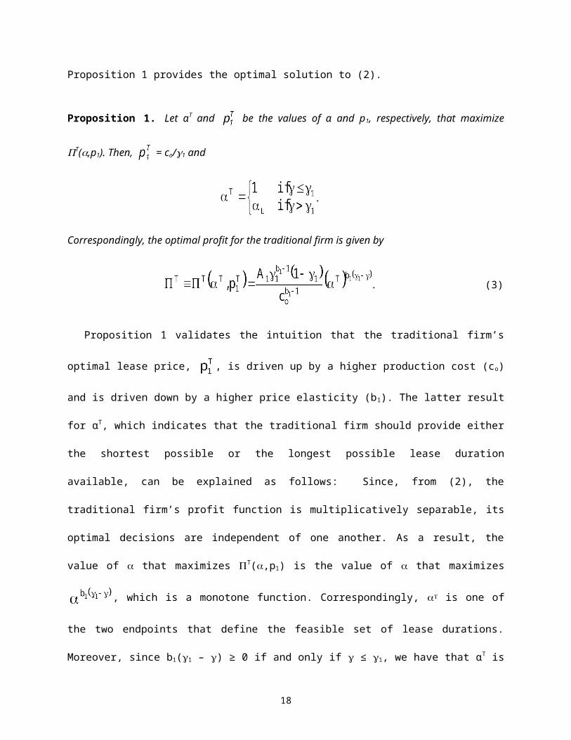
Proposition 1 provides the optimal solution to (2).

Proposition 1. Let αT and be the values of α and p1, respectively, that maximize T(,p1). Then, =

co/1 and

.

Correspondingly, the optimal profit for the traditional firm is given by

. (3)

Proposition 1 validates the intuition that the traditional firm’s optimal lease price, , is driven up by

a higher production cost (co) and is driven down by a higher price elasticity (b1). The latter result for αT,

10

which indicates that the traditional firm should provide either the shortest possible or the longest possible

lease duration available, can be explained as follows: Since, from (2), the traditional firm’s profit

function is multiplicatively separable, its optimal decisions are independent of one another. As a result,

the value of that maximizes T(,p1) is the value of that maximizes , which is a monotone

function. Correspondingly, is one of the two endpoints that define the feasible set of lease durations.

Moreover, since b1(1 – ) ≥ 0 if and only if ≤ 1, we have that αT is non-increasing in . Intuitively,

this result follows because, for a larger , customers extract sufficient value early in a lease cycle so that

they are willing to have shorter lease cycles for the same price. Finally, by (3), Proposition 1 also

indicates that the traditional firm’s optimal profit is increasing in , which is consistent with the intuition

that the higher is the rate by which customers extract value from a product, the more is the overall value

that the traditional firm can extract from the market.

4. GREEN FIRM’S OBJECTIVE FUNCTION

We define a green firm as one that not only can produce items for lease in the lease market, but also can

remanufacture them upon their return for sale in a separate remanufactured goods market (secondary

market). The assumption of a separate secondary market has precedence in the literature (see, for

example, Guide et al. 2003, who assume a third-party remanufacturer that acts as a monopolist).

Moreover, empirical and anecdotal support for this assumption can be found in Atasu et al. (2010) and in

Guide and Li (2010). Like the traditional firm, the green firm chooses its optimal lease price and lease

duration, but unlike the traditional firm, the green firm also determines an optimal design for the

remanufacturability of its product as well as the optimal quantity of after-lease items to remanufacture.

In this section, we formulate the green firm’s objective function after first describing the

remanufacturing process and secondary market. We begin by defining the following:

K (Ko ≤ K ≤ 1) Product design decision variable representing the fraction (i.e., percentage)

of a green product that is remanufacturable. The parameter Ko is exogenous and

11

represents the minimum level of remanufacturability that is required for remanufacturing

a used product. Such a requirement might be due to technology, capacity, or regulation.1

co(1 – K) The per-unit cost (in, e.g., $/unit or €/unit) of producing the non-remanufacturable

fraction of a green product, where, for consistency, co is equivalent to the per-unit

production cost of a traditional product, as defined in Section 3.

ciK The per-unit cost (in, e.g., $/unit or €/unit) of producing the remanufacturable fraction of

a green product. We assume that ci > co to reflect that, everything else being equal, it

costs more to produce a unit of a remanufacturable product than it does to produce a unit

of a traditional one.

crαK The per-unit cost (in, e.g., $/unit or €/unit) of remanufacturing the remanufacturable

fraction of an after-lease (i.e., used) product. We assume that this cost is increasing in

to reflect that, everything else being equal, a unit that is used longer in the lease market

costs more to remanufacture (i.e., restore to its original condition) upon its return; and we

assume that cr < co to reflect that, everything else being equal, remanufacturing an after-

lease unit is less expensive than producing that unit from scratch.

The product design decision variable K is related to how much of the product is designed to be

remanufacturable. For example, in the case of mobile phones, K = 1 would mean that the entire phone can

be remanufactured while K < 1 means a portion of the phone can be remanufactured. The costs c o, ci, and

cr can be determined by the design requirements in each case, and would depend on the additional

modularity that might be needed for easier disassembly, different materials to be used for the

remanufacturable components, etc.

Given these definitions, we specify the cost of producing one unit of the green product as c1(K) ciK

+ co(1 – K), and we specify the cost of remanufacturing one after-lease unit of the green product as

1 The existence of Ko also rules out the case where the green firm has access to two markets (new and

remanufactured goods) without making an additional investment to the one the traditional firm is making. This

eliminates an uninteresting comparison as the green firm will certainly be at an advantage.

12

c2(K,α) crαK + co(1 – K). In this specification of the per-unit remanufacturing cost, we assume that the

cost of the non-remanufacturable portion of the unit, (1 – K)co, to be at the same unit cost rate (co) as the

original production of that portion of the unit because, by the definition of K, that portion must be

replaced with original components. Moreover, we assume that both c1(K) and c2(K,) are linear in K to

capture the interactions between the design and the sales contract decisions while making our model

analytically tractable.

Analogous to the lease-market demand represented by (1), we assume that the demand in the

secondary market (representing the market faced by the firm without any competitive concerns) is

where b2 is the price elasticity of the secondary market demand and A2 is a parameter

reflecting the size of the secondary market that relates the per-unit selling price of a remanufactured good

(p2) to the total units demanded in the secondary market. We also define 2 = (b2 – 1)/b2 to be analogous

to 1. Note that the demand for remanufactured goods is only price-sensitive; it does not depend on the

remanufacturability of the item (K) or on how long the product was used in the lease market before its

return (). This is because we captured such effects above, in our formulation of the per-unit

remanufacturing cost function. In particular, we implicitly assumed that the remanufacturing process

restores a given after-lease unit of the green product to a condition acceptable to the secondary market at

a cost that is a function of α and K so that there is no effect on market perception of the product with

regard to these decision variables. This is also in line with a market of consumers that is functionality-

oriented, that would have more of an interest in whether an item “works” rather than in whether it is new.

Let Q2(α,p1,p2) denote the quantity of units of the remanufactured product sold in the secondary

market. Because this quantity is constrained by the total number of after-lease units available for

remanufacturing, which is equal to the total quantity of units demanded by the lease market over the

planning horizon, we have

.

13

For convenience, we let Q2 denote the green firm’s decision variable in lieu of p2, and thus set p2

implicitly by the selection of Q2. Accordingly, we require Q2 ≤ D1(α,p1) and let . As a

result, the green firm’s objective, which is to maximize its combined profits from the lease market and the

secondary market, can be written as follows:

(4)

. (5)

Given a set of values (α,p1,Q2), we define the firm to be “supply constrained” if (5) is binding and

“market constrained” if (5) is not binding. For instance, if a mobile phone manufacturer has more demand

for remanufactured phones than it has used phones available, it will be supply constrained while if the

market for remanufactured phones is smaller than the number of used phones available, it will be market

constrained. This distinction will be useful for characterizing the optimal decisions of the green firm and

their implications for profits and environmental friendliness.

Note that the objective function (4) reflects several tradeoffs. First, a larger K means a higher

production cost for new units, but a lower remanufacturing cost for after-lease units. Second, a larger α

increases remanufacturing costs, but also has the potential to increase lease market demand. Finally, a

large A2 or a small cr (or both) creates an incentive to produce more in the lease market in order to

increase the supply of after-lease items available for the secondary market, however the higher production

in the lease market would then drive down the price in that market.

14

5. GREEN FIRM’S OPTIMAL SOLUTION

In this section, we develop an algorithm to establish and to characterize the green firm’s optimal solution.

Then we implement that algorithm in an exploratory numerical study to generate insights into the optimal

behavior of the green firm, and to lay the groundwork for our comparison of the green firm with the

traditional firm in Section 6.

To establish the optimal solution, we proceed in several steps as summarized by Figure 2. (In Figure

2 and throughout, we use the notation xG() to represent the green firm’s optimal decision for x, given

that the decision variables in () are fixed.) We begin with Proposition 2 to establish that the decision

space for KG, the optimal K for the green firm, can be reduced to two points, namely K o and 1. Then, in

Section 5.1, we solve for and , the optimal values of Q2 and p1, respectively, for a

given α and K. By substituting for Q2 and for p1 in G(α,,p1,Q2), we thus reduce

the characterization of the green firm’s expected profit to a function of only α and .

Next, in Section 5.2, we solve for αG(K) in three steps by analyzing the resulting market- and supply-

constrained expected profit functions separately as follows: First, we divide the domain for α into a

market-constrained region, which is implicitly defined by the values of α that satisfy the condition

< , and a supply constrained region, which is implicitly defined by the values

of α that satisfy the condition = . Second, given these two regions, we

determine and as the values of α that maximize expected profit for a given K over each of

these two respective regions. And third, we establish αG(K) by comparing G( ,) to G(

,), where G(,) .

Given αG(K), we then reduce the green firm’s expected profit to a function of the single variable K by

substituting αG(K) for in G(,). Therefore, to complete the green firm’s optimal solution, we can

determine KG by computing and comparing G(G(KG)KG) for K = Ko and K = 1, which represent the two

15

possible values of KG as per Proposition 2. Given KG, the green firm’s optimal , p1, and Q2 are,

respectively, G = (KG), , and .

------------------------------

Insert Figure 2 here

------------------------------

As per Step 1 of Figure 2, given that KG is defined as the value of K that maximizes G(α,K,p1,Q2),

we establish Proposition 2 to reduce the candidate space for the optimal K to two points.

Proposition 2. KG {Ko,1}.

Proposition 2, which is a direct consequence of the linear per-unit cost functions for manufacturing and

remanufacturing, helps to derive insights by simplifying the solution procedure of the green firm’s

maximization problem.

5.1 Optimal Q2 and p1 for a green firm, given K and α

In Proposition 3 we characterize and , the values of Q2 and p1, respectively, for a

given α and K, that maximize G(α,K,p1,Q2), and we establish their uniqueness.

Proposition 3. For given values of K and , let be the unique value of p1 that solves

.

Moreover, let , , and . Then, the

following table characterizes and :

If… then, = and =

16

Notice from (1) and the definitions of and that .

Therefore, Proposition 3 indicates when the green firm is market or supply constrained, for any given α

and K. In particular, if = , then the green firm is market

constrained, and if = , then the green firm is supply

constrained.

Interpreted in the context of the given market and cost parameters, this result has several implications.

For example, it means that higher values of drive the green firm toward a market constrained

remanufacturing policy and away from a supply constrained one. The reason for this is because,

everything else being equal, D1(,pm(K)) is increasing in , while Qm(,K) is independent of . Higher

values of cr also drive the green firm toward a market constrained policy, but for a different reason:

Qm(,K) is decreasing in cr while D1(,pm(K)) is independent of cr. In contrast, higher values of ci drive

the green firm toward a supply constrained policy, which is because D1(,pm(K)) is decreasing in ci while

Qm(,K) is independent of ci. The effect of co, however, is ambiguous because both Qm(,K) and

D1(,pm(K)) are decreasing in co. Given this ambiguity, we explore the effects of co further in Section 5.3

as part of our numerical study of the green firm’s optimal policy. These findings are consistent with

observations from the mobile phone market (with high levels of γ; see for example Jang and Kim (2010)),

where operators or manufacturers will remanufacture a fraction of the used phones they collect (examples

from practice can be found in Jang and Kim (2010), Srivastava (2004), Tanskanen and Butler (2007)),

thus operating in a market-constrained environment.

17

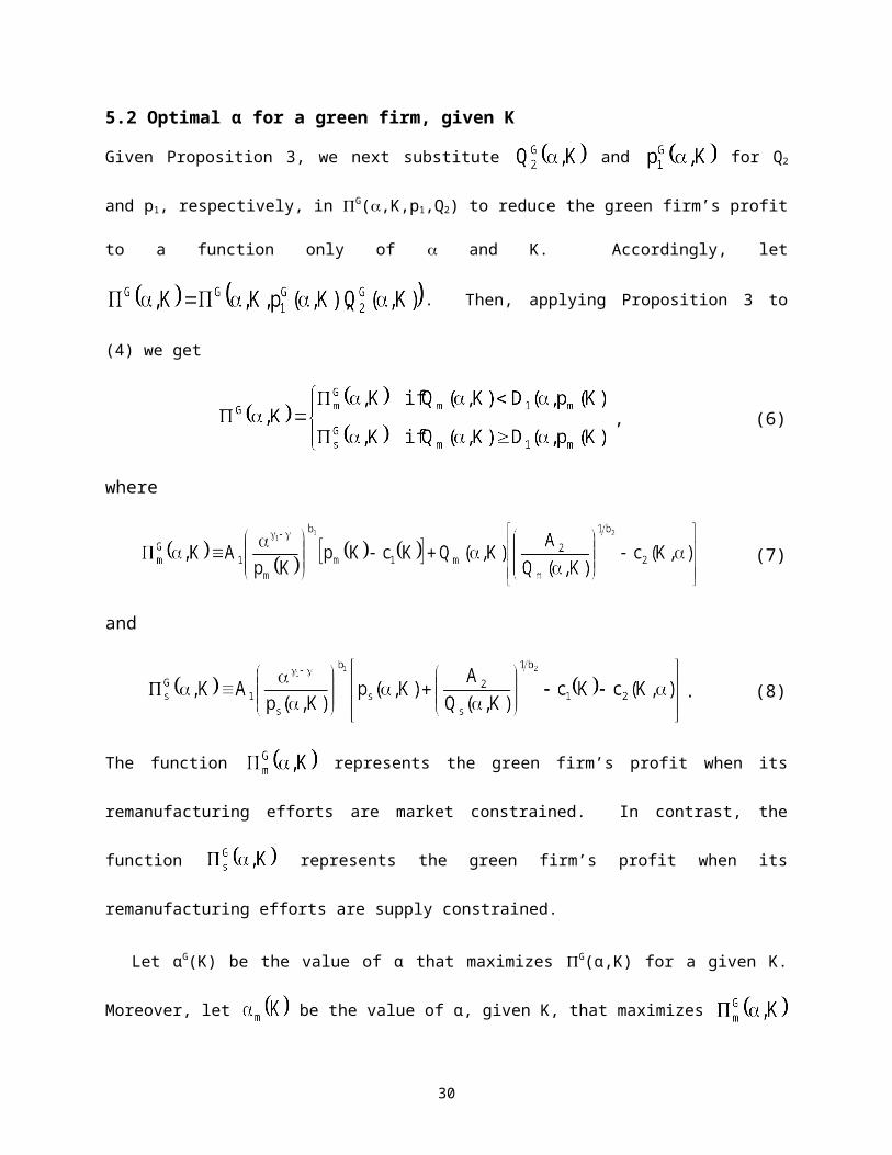
5.2 Optimal α for a green firm, given K

Given Proposition 3, we next substitute and for Q2 and p1, respectively, in

G(,K,p1,Q2) to reduce the green firm’s profit to a function only of and K. Accordingly, let

. Then, applying Proposition 3 to (4) we get

, (6)

where

(7)

and

. (8)

The function represents the green firm’s profit when its remanufacturing efforts are market

constrained. In contrast, the function represents the green firm’s profit when its

remanufacturing efforts are supply constrained.

Let αG(K) be the value of α that maximizes G(α,K) for a given K. Moreover, let be the value

of α, given K, that maximizes subject to the constraint , and let

be the value ofα, given K, that maximizes subject to the constraint

. Then, for any given K, G(K) = m(K) represents the scenario in which it

is optimal for the green firm to establish a market-constrained remanufacturing operation, and G(K) =

s(K) represents the scenario in which it is optimal for the green firm to establish a supply-constrained

remanufacturing operation.

The primary question of this section is whether the green firm will have a market-constrained or a

supply-constrained remanufacturing operation, i.e., G(K) = m(K) or G(K) = s(K). However, a

18

secondary question is how to characterize G(K). To those ends, we analyze (6) – (8) differently

depending on whether 1 or < 1. In either case, however, the following lemma provides the

fundamental building block.

Lemma 1. G(,K) is continuous and differentiable as a function of , for L ≤ ≤ 1.

Given Lemma 1, we first consider the case in which 1. For this case, we address the questions

of this section directly, by first determining G(K) explicitly, and then by verifying whether that

determined value corresponds to a market- or a supply-constrained solution. We characterize the results

of this analysis with Proposition 4.

Proposition 4. If ≥ 1 then G(K) = αL. Accordingly, G(K) = m(K) if Qm(L,K) < D1(L,pm(K)), and

G(K) = s(K) if Qm(L,K) ≥ D1(L,pm(K)).

Proposition 4 follows because, from (7) and (8), both and are non-increasing in α if

1. Combined with Lemma 1, this implies that G(K) = αL. Basically, if ≥ 1, then a lower α leads

both to a higher demand in the lease market (and thus a higher supply for the secondary market) and to a

lower per-unit cost of remanufacturing.

We next consider the case in which < 1. For this case, we address the questions of this section

indirectly by first characterizing m(K) and s(K), and then by applying those characterizations to

determine αG(K) implicitly. This approach is validated, in effect, by the observation that m(K) and s(K)

each can be determined by searching over a single complementary interval. To demonstrate this, notice

from Proposition 3 that Qm(,K) is decreasing in α and that D1(,pm(K)) is increasing in α if < 1.

Consequently, if < 1, then, for a given K, Qm(,K) – D1(,pm(K)) is decreasing in , which implies that

there exists no more than one value of α that satisfies Qm(,K) – D1(,pm(K)) = 0. Accordingly, let

denote that value of α, if it exists. Otherwise, let 0(K) = 0 if Qm(,K) – D1(,pm(K)) < 0 for all ; or let

0(K) = if Qm(,K) – D1(,pm(K)) > 0 for all . Then G(K) can be characterized in terms of m

and s as follows:

19

Proposition 5. For < 1, and for a given K:

(i) If 0(K) < L, then Qm(,K) < D1(,pm(K)) for all [L,1], which implies G(K) = m(K);

(ii) if L ≤ 0(K) < 1, then Qm(,K) < D1(,pm(K)) if and only if >0(K), which implies G(K) = argmax{ , }, where m(K) (0(K),1] and s(K) [L,0(K)];

(iii) if 1 ≤ 0(K), then Qm(,K) ≥ D1(,pm(K)) for all [L,1], which implies G(K) = s(K).

In other words, if < 1, then Proposition 5 together with Lemma 1 establishes that, for a given K,

G(K) can be determined as follows: first, maximize over the interval [L,min{0(K),1}] to

determine s(K); second, maximize over the interval [max{L,0(K)},1] to determine m(K);

and, third, compare with to determine G(K). Thus, in principle, the

determination of G(K) can be characterized as a three-step procedure when < 1; but, that procedure

effectively reduces to a single step if either of the two specified intervals is empty.

Given the search procedure implied by Proposition 5, we next complete the specification of G(K) by

characterizing m(K) and s(K). To that end, we introduce Proposition 6, which ultimately reduces the

search for m(K) and s(K) to two sets of specified candidate values.

Proposition 6. For < 1, and for a given K,

(i) , where satisfies the equation

.

(ii) , where satisfies the equation

.

20

Since Propositions 5 and 6 characterize the green firm’s optimal α for a given value of K, and since

Proposition 2 restricts KG to be one of only two possible values, this completes the validation of the green

firm’s solution procedure presented earlier in Figure 2. Next, in Section 5.3, we apply this solution

procedure in a comprehensive numerical study to develop deeper insights into the resulting solution,

particularly with respect to what drives the green firm’s product design decision and its corresponding

decision to establish either a market-constrained or a supply-constrained remanufacturing operation.

5.3 A numerical exploration of the green firm’s optimal solution

With this numerical study, we primarily focus on two dimensions of the green firm’s optimal

remanufacturing policy. First, we explore when KG = 1 vs. when KG = Ko to yield insights into the issue

of whether or not it is optimal for the green firm to design a product that is fully remanufacturable.

Second, we define the measure RG = as the proportion of after-lease items that are

remanufactured and we explore when RG = 1 vs. when RG < 1 to yield insights into the issue of whether or

not it is optimal for the green firm to establish a remanufacturing volume that is supply constrained.

Determining conditions that lead to KG < 1 and/or RG < 1 is particularly interesting because these

measures have implications for the environment. For example, an optimal policy in which KG = Ko can

be interpreted as an unwillingness on the part of the green firm to commit fully to remanufacturing.

Similarly, a policy in which RG < 1, which indicates that it is optimal for the green firm to remanufacture

fewer units than it has available to remanufacture, might signal possible inefficiencies in the

remanufacturing market or the remanufacturing process.

In addition to analyzing KG and RG, we use this section to perform sensitivity analyses on the green

firm’s optimal profit, prices, and lease duration. These analyses lay the foundation for Section 6, which is

dedicated to comparing the efficacy of the traditional firm’s and the green firm’s optimal policies in terms

of profit and environmental friendliness.

To implement the numerical study of this section, we applied the solution procedure from Figure 2

for all combinations of the parameter values listed in Table 2 (a total of 21,546 combinations in all). In

21

composing Table 2, we chose values of and b1 such that = - 1 corresponds to a case in which < 0,

= 0.15 corresponds to a case in which 0 < ≤ 1, and = 0.8 corresponds to a case in which 1 < ≤ 1. In

addition, we chose values of A1 and A2 such that both A2 > A1 and A1 > A2 can be explored so as to

develop a deeper understanding of how the scale of the secondary market relative to the scale of the lease

market might affect the green firm. Note that A2 > A1 can be interpreted to mean generally that the scale

of the secondary market is comparatively larger relative to the lease market, whereas A 1 > A2 can be

interpreted to mean generally that the scale of the secondary market is comparatively small relative to the

lease market.

Table 2: Scope of Numerical Exploration

Parameter Values # of values

cr 1, 10 2

ci/cr 1.2, 2, 3 3

co cr + n(ci - cr)/20, n = 1, 2, …, 19 19

b1 1.2, 1.4, 1.8 3

b2 1.2, 1.4, 1.8 3

A2/A1 0.25, 0.5, 0.75, 1, 1.25, 1.5, 3 7 -1, 0.15, 0.8 3

Figure 3 plots KG and RG as functions of co. Note that there are two possible scenarios for KG, labeled

S1 and S2. In scenario S2, KG = Ko when co is below some threshold value (identified in Figure 3 as ),

and KG = 1 when co is equal to or greater than that threshold value. However, in scenario S1, KG = 1 for

all co. For each of these two scenarios, there then are two possible scenarios for R G. For example, if KG =

1 for all co (scenario S1), then either RG = 1 for all co (scenario S1a) or RG < 1 for all co (scenario S1b).

------------------------------

Insert Figure 3 here

------------------------------

22

In terms of product design, Figure 3 indicates that KG is non-decreasing as a function of co. This is

intuitive because as co increases, the difference between the cost of producing a product with K < 1 vs. K

= 1 diminishes. Therefore, the savings in the cost of remanufacturing eventually outweighs the additional

cost of producing a more remanufacturable product. In terms of remanufacturing volume, if K G = 1, then

the per-unit cost of the green product is independent of co, thus co does not influence RG (as per scenarios

S1a and S1b). However, if KG = Ko, then co does influence RG (as per scenarios S2a and S2b). This case

is particularly interesting because it indicates that RG first decreases (beginning at a threshold value that

we identify as C) and then increases as co increases. One way to explain this is as follows: When KG =

Ko, RG starts to decrease as co increases because the per-unit remanufacturing cost increases accordingly,

and this makes remanufacturing less appealing. Nonetheless, recall from Figure 3 that a higher c o also

drives the optimal product design decision up from KG = Ko to KG = 1, and this switch puts downward

pressure on the per-unit remanufacturing cost. This in turn makes remanufacturing more appealing, thus

creating upward pressure on RG. Finally, once co is such that KG = 1 (i.e., when co ≥ ), co ceases to

affect RG for the same reason as in scenario S1. In practical terms, this suggests that the cost structure of

the product needs to be taken into careful consideration to understand the effect of having a

remanufacturable product on the volume and quality of remanufacturing, and that certain cost structures,

especially those in which there are considerable differences in processing new, remanufacturable, and to-

be-remanufactured components, can have counter-intuitive negative impacts. For example, one of the

insights from these experiments is that while low cost (co) encourages minimum remanufacturable design

and full remanufacturing when the products are returned, at medium values of the cost, not all products

are remanufactured and resold in the secondary market.

In Figure 3, for scenarios S2a and S2b, we should also note that it is possible that the drop in RG

below RG = 1 might not occur. This tends to be true when conditions are favorable for remanufacturing,

for instance if A2 is larger rather than smaller. Alternatively, for these scenarios it is also possible that R G

< 1 when co cr if conditions are unfavorable for remanufacturing, for instance if cr is large.

23

Given that KG is non-decreasing as a function of co, a smaller rather than larger value of co is

necessary for KG = Ko. However, as evidenced by the existence of scenario S1, a small co is not sufficient

for KG = Ko; instead, one or more of several other conditions are also required. For example, we found

that KG = Ko when a small co is coupled either with a large ci/cr ratio or with a very small . Intuitively,

KG = Ko when co is small and ci/cr is large because, under such circumstances, setting K = 1 would create

excessive production costs in the lease market without providing commensurate savings in

remanufacturing costs.

The link between and KG is similar, but less direct. Basically, we find from our numerical study

that G, the green firm’s optimal , is non-increasing as a function of . (This is depicted later in Table 3

as part of the sensitivity analysis, and it is consistent with Proposition 1, which establishes that the

traditional firm’s optimal also is non-increasing as a function of .) As a result, G becomes larger as

becomes smaller, which in turn translates into a higher per-unit remanufacturing cost. This, combined

with a low co, yields KG = Ko because, under such circumstances, setting KG = 1 would not provide

enough savings in remanufacturing costs to offset the corresponding increase in production costs. These

results suggest that an advantageous cost structure is not necessarily required to have a fully

remanufacturable product in optimality, and that the firm has to consider the inherent nature of the

product and lease market. One insight for managers is that when the cost of the core is low and the value

of the product is realized later in its life, even small cost to remanufacture may not be enough for a firm to

adopt remanufacturing.

Note that the circumstances that lead the green firm to choose KG = Ko have significance for the

environment if other parameters are favorable for supporting a higher remanufacturing volume (e.g., a

larger rather than smaller A2/A1 ratio). This is because a high level of remanufacturing volume, when

coupled with a low level of remanufacturability, has negative implications for the environment in the

form of an overabundance of discarded components. We further discuss this issue in Section 6.3.

Not reflected in Figure 3 is one more observation also worth noting: The optimal amount of

remanufacturing activity for the green firm, whether reflected in the form of KG or RG, is typically highest

24

for values of that are close to 1. To help explain this phenomenon, recall from the discussion above

that G is non-increasing as a function of , and recall from Proposition 4 that G = L when 1.

Accordingly, on the one hand, if < 1, then a smaller corresponds to a larger G, which implies a

larger per-unit remanufacturing cost, thus creating a deterrent for remanufacturing activity. On the other

hand, if > 1, then a larger corresponds to a higher lease market demand, which makes it less

economically viable to remanufacture everything originally produced, thus creating a second deterrent for

remanufacturing activity. In contrast, as approaches 1, lease market demand becomes less sensitive to

α, which allows the green firm to choose a small α to reduce remanufacturing costs without creating an

excessive surge in lease market demand. Therefore, customer expectations and the ability of customers to

extract value earlier from products in the lease market, although positively linked to more

remanufacturable product design, and to profitability in general, can have adverse impacts on what

proportion of goods are remanufactured upon return. This is similar to the effect of A 2/A1 described

above, and will be discussed further in Section 6.3.

We conclude this section by providing a sensitivity analysis, in Table 3, of the optimal values of the

remaining decision variables as well as the optimal profit of the green firm. In Table 3, “+” means that

the variable listed in the row of the table is non-decreasing as a function of the parameter listed in the

column of the table, “-” means that the variable is non-increasing as a function of the parameter, “+/-”

means that the variable is first non-decreasing and then non-increasing as a function of the parameter, and

so on.

25

Table 3: Sensitivity Analysis

co ci cr b1 b2 A2/A1

G - - - - - n/a2 +

G +/- + - + - or +1 - -

+ + + - - - -/+/-

+/- + + + - + -/+

1αG is increasing in b2 for large cr and decreasing in b2 for small cr.2 G is increasing in both A1 and A2.

Table 3 has several implications for customers in particular. First, we observe that, generally

speaking, optimal prices ( and ) are non-decreasing in costs (co, ci, and cr) and non-increasing in

price elasticities (b1 and b2), which are intuitive results. Nevertheless, we also observe that, as exceptions

to that general rule, is non-decreasing in b1 and, potentially, it also could be non-increasing in co.

These exceptions are because although the green firm’s market for remanufactured goods is independent

of its lease market for new goods, its operations in the two markets are nonetheless linked because the

volume of new items leased on the one market constrains the volume of remanufactured items that can be

sold on the secondary market. Thus, for example, a higher b1 ultimately could translate into a reduced

volume of leased items available for remanufacturing, which in turn provides license for the green firm to

increase . For example, if purchasers of new mobile phones are price-sensitive (high b 1), this could

explain why, as described above, mobile phone remanufacturers are market-constrained (p 2 too high to

clear the market). Therefore, it is interesting to note that customers in one market, through their behavior,

can influence outcomes for customers in a seemingly independent market, in turn influencing the firm’s

ability to benefit from remanufacturing operations.

6. A COMPARATIVE STUDY OF GREEN FIRM VS. TRADITIONAL FIRM

In this section, we utilize our algorithm of Section 5 to numerically compare the optimal policy of a

traditional firm to the optimal policy of a green firm using two measures of efficacy: (i) profit, and (ii)

26

environmental friendliness. We apply the first measure, profit, to investigate the conditions under which it

is profitable for a firm to be a remanufacturer. We apply the second measure, environmental friendliness,

to examine the impact of remanufacturing on the environment. We compute this measure by comparing

the volume of after-lease components discarded by the green and traditional firms. In Section 5, we

explored KG and RG, which, taken alone, are indicative of the proportion of components discarded by the

green firm. The volume of components discarded is a composite of these separate measures as it considers

both product design and the quantity remanufactured. Naturally, by definition, because of its product

design decision, the green firm has a better per-unit environmental position. However, the volume

discarded is also important because the green firm’s discarded volume can actually be more than the

traditional firm’s discarded volume, depending on the relative sales of the two firms in the lease market.

In the following sections, we present results of a numerical study of the green and traditional firms

with respect to the measures presented above. As inputs, we apply the same parameter values used in

Section 5.3 and itemized in Table 2. In presenting the results of this study, unless otherwise noted, we

use as a representative illustration the case in which A2/A1 = 0.25, = 0.8, cr = 1, and ci = 3.

6.1 Green vs. Traditional: Optimal Profit Comparison

In this section, we compare the green and traditional firms in terms of their profits. Let G = G(αG,

,KG, ) and T = T(αT, ). Then, G/T represents the ratio of the green firm’s optimal profits to the

traditional firm’s optimal profits for any given set of parameters.

Figure 4 illustrates the typical behavior of G/T as a function of co. Notice that the traditional firm

is more profitable than the green firm if co is below a certain threshold value whereas the green firm is

more profitable if co is above that threshold value. Intuitively, this is because a low co, as discussed in

Section 5.3, means that the benefit from remanufacturing is not sufficient to justify the expense of

producing a more remanufacturable product. Nevertheless, the more favorable are other parameters for

remanufacturing (for example, the higher is A2/A1 or the lower is ci/cr), the lower is this threshold value,

thereby increasing the relative profitability of the green firm vis-à-vis the traditional firm. From Figure 4,

27

we also observe that G/T is decreasing as a function of b2. Intuitively, this is because a larger b2, which

signifies a higher price elasticity for the secondary market, means that the green firm will have to lower

its price in the secondary market to generate the same amount of demand. This suggests that a higher cost

for the core product and a relatively price-insensitive secondary market is in the interest of the

remanufacturer.

------------------------------

Insert Figure 4 here

------------------------------

Although not depicted in Figure 4, the results of our numerical study also suggest that, everything

else being equal, G/T is highest when 1, which means that the traditional firm has the best chance

of being more profitable than the green firm for smaller or larger values of . This result is expected

given the behavior of the green firm with respect to as described in Section 5.3, where we discussed that

the green firm’s remanufacturing activity is less if is not close to 1. This result suggests that

remanufacturing is more profitable as a strategy if the primary consumer market is less sensitive to

changes in contract conditions. For instance, given the sensitivity of mobile phone consumers to contract

conditions, it is not surprising that typically RG < 1 for OEMs that remanufacture mobile phones (Jang

and Kim (2010), Srivastava (2004), Tanskanen and Butler (2007)). Intuitively, this is because such in-

sensitivity allows the firm to adjust the contract to fit the requirements of the remanufacturing operation,

without losing too much ground in the primary market.

6.2 Green vs. Traditional: Environmental Friendliness Comparison

In this section, we compare the green and traditional firms in terms of their environmental friendliness. In

this context, we measure environmental friendliness by computing the total volume of after-lease discards

28

over the planning horizon, and we say that the smaller is the amount discarded, the more environmentally

friendly is the firm2.

By definition, the traditional firm uses resources to produce products, all of which are then discarded.

In contrast, the green firm discards only a portion of after-lease items and reuses the rest. In particular, the

green firm uses resources to produce D1 units in the first period, and in the second period it uses

additional resources to produce KQ2 units/components with the remainder of production, (1 – K)Q2,

coming from the remanufacturable components of the returned products. Accordingly, let L i be the total

amount of components that is discarded by Firm i (for i = T, G), given that the firm follows its profit-

maximizing policy. Then,

LT =

.

In Figure 5, we present an illustrative example of LG/LT as a function of co. In this example, LG/LT < 1

for all co, which indicates that the green firm is more environmentally friendly than is the traditional firm

for all values of co. This supports the idea that firms can turn to remanufacturing if they want to be

considered as being more environmentally friendly. However, recall from Figure 4 that, everything else

being equal, the traditional firm is more profitable than the green firm for small values of co. As a result,

for such values of co, the environment gets shortchanged in terms of the overall volume of components

discarded. Indeed, when co is close to cr, LG/LT 0.5, which means that the firm type with the higher

2 Note that we focus on the environmental damage associated with not being able to utilize the products in any way

after they are used and returned in the primary market. In the absence of remanufacturing, all returned products are

discarded and sent to landfill. We are interested in the reduction in the amount going to landfill by being reused

productively in another product. Thus, we do not include the eventual discarding of the remanufactured products in

our definition of environmental friendliness above, as we tacitly assume that “after-lease” discards are more

damaging to the environment than are “post-secondary market” discards. All things considered, the more premature

the discard, the more damaging is the effect to the environment (given that a new item will need to be produced to

replace the item discarded).

29

profit (traditional) discards approximately twice as much material as the more environmentally friendly

firm (green) would discard.

------------------------------

Insert Figure 5 here

------------------------------

Figures 4 and 5 together demonstrate that there exist situations in which the traditional firm can earn

higher profit while the green firm is more environmentally friendly. For example, when the cost of

producing a traditional product is moderate, the green firm is more profitable and has a higher level of

environmental friendliness compared to the traditional firm. However, situations exist in which the

opposite is true as well. For example, consider Figure 6, where A2/A1 = 3 and = 0.15. Notice that

although the green firm is more profitable than the traditional firm for all values of co, there exists a range

of co values for which the traditional firm is more environmentally friendly than the green firm. To

explain this phenomenon, note that when there is an opportunity for a large volume of sales in the

secondary market, this opportunity translates into increased sales in the lease market. However, as

discussed in Section 5.3, under certain conditions the green firm will set KG = Ko when co is small,

regardless of how large the secondary market is. As a result, the volume of un-remanufacturable

components that the green firm discards could far exceed the volume of non-remanufacturable items

discarded by the traditional firm.

------------------------------

Insert Figure 6 here

------------------------------

30

6.4 Synthesis and Discussion

Given the nature of the results illustrated by Figures 4-6, in this section we describe conditions under

which the more profitable firm indeed is the more environmentally friendly firm, as well as conditions

under which the more profitable firm is the less environmentally firm. To summarize these conditions,

we use Table 4 to identify which firm (T or G) earns higher profit (P) and which is more environmentally

friendly (EF), as functions of co and A2/A1, given that each firm follows its profit-maximizing policy.

Table 4: Synthesis of Results

co

small (1-2) medium (2.5-7.5) large (8-10)

P EF P EF P EF

A2/A1

small (0.25-0.5) T G T,G1 G G G

medium (0.75-1.25) G G G G G G

large (1.5-3) G T,G2 G T,G2 G G1 If b1 > b2, then T is more profitable; if b1 < b2, then G is more profitable. If b1 = b2, then T is more profitable for values of co below a certain threshold, whereas G is more profitable for values of co above that threshold.2 For relatively medium values of b1, G is more environmentally friendly. However, for either relatively small or relatively large values of b1, T is more environmentally friendly if b2 is below some threshold, and G is more environmentally friendly if b2 is above that threshold.

As Table 4 indicates, as a general rule, the green firm is more profitable as well as more

environmentally friendly than is the traditional firm. However, if A2/A1 is relatively small or relatively

large, then there is a possibility that the traditional firm will be either more profitable or more

environmentally friendly (but not both) as compared to the green firm, depending on the values of c o and

b2/b1. This can be explained as follows: first, a lower A2/A1 is indicative of a relatively smaller scale

secondary market, in which case the secondary market simply may not be of sufficient scale to justify

producing a remanufacturable product, thus creating the opportunity for the traditional firm to be more

profitable. Second, a higher A2/A1 is indicative of a relatively larger scale secondary market, in which

case the green firm very well might have the inventive of increasing production in the lease market

31

simply to increase its capacity to remanufacture and sell more in the secondary market. As demonstrated

in Section 6.2, this in turn could lead to an excessive volume of discarded components.

In addition to these observations, we found profit to be increasing as a function of for both firms

(which is consistent with Table 3). Intuitively, this happens because, recall, larger values of are

representative of higher rates of value extraction by customers, everything else remaining equal. Thus,

consistent with Sections 3 and 5, a larger leads to shorter optimal lease durations, which in turn leads to

an increase in lease frequency and thus, profits, over the fixed planning horizon. However, under such

circumstances, there is a risk that the increased lease frequency will hurt the environment, especially if

the secondary market is not large enough to support the increased volume generated by the lease market.

A product type that may have a large is a cell phone or an automobile, since the customer perception of

the value of a new item is rapidly decreasing once it has been purchased. In contrast, when is small,

because the discard volume is small for both firm types, the cost to the environment will not be too high

when the more profitable strategy is selected, even if it is not the more environmentally friendly strategy.

Recall that a small value of ( < 0) corresponds to a rate of value extraction that is increasing over time.

This is the case for many products with a learning curve, for instance most industrial machinery would fit

into this category.

In summary, meeting the twin objectives of profit and environment friendliness requires the firm to

make sure that the products it offers provide to the customer high value soon after they start using the

product and that there is a moderate size market for remanufactured products. Otherwise the firm has to

compromise on at least one of the twin objectives.

7. SUMMARY AND EXTENSIONS

In this paper, we developed, solved, and analyzed a model to explore conditions under which

remanufacturing is profitable. Moreover, by comparing the optimal policies of a green and a traditional

firm, we investigated how remanufacturing, given that it is profitable, affects the environment.

32

In this context, we found that the green firm typically generates a higher profit and is more

environmentally friendly than is the traditional firm. Nonetheless, we also found that exceptions exist to

this general rule. For example, we identified two scenarios under which the traditional firm outperforms

the green firm along one or both of these performance measures: First, if the scale of the secondary

market is small relative to the scale of the lease market, then the traditional firm will be more profitable

than the green firm, although the green firm will be more environmentally friendly than the traditional

firm. Second, and perhaps more interestingly, if the scale of the secondary market is large relative to the

scale of the lease market, then the traditional firm could be more environmentally friendly than the green

firm. Intuitively, this phenomenon occurs because the green firm’s optimal response in such

circumstances would be to design a product that minimally meets the requirements for remanufacturing.

This opens a second market (namely, the secondary market) to the green firm, which in turn leads the

green firm to produce more units than the traditional firm for sale in the lease market. Ultimately, this

translates into the green firm collecting and discarding a larger volume of non-remanufacturable

components from after-lease units.

This paper contributes to the remanufacturing literature in several ways. First, at the conceptual level,

it contributes to an understanding of what drives remanufacturing and under what conditions

remanufacturing accomplishes environmental efficiency. Second, at the operational level, it provides a

framework for incorporating product design into a remanufacturing decision model. Third, it explicitly

accounts for interactions between product properties such as value extraction or production costs and

market properties such as price elasticity or the relative scale of a market. Moreover, by developing a

cost-benefit analysis of remanufacturing, this paper provides insight into the issue of whether or not

remanufacturing is worth the effort, and it assesses the extent to which profit-maximization translates into

increased environmental friendliness. As such, it provides insights not only for green firms, but also for

regulators and policy makers interested in inducing firms to become greener.

One can build on these contributions through several extensions. First, in order to more fully explore

the role of lease-contract flexibility, it would be interesting to extend our model to a case in which each

33

customer is given the freedom to select her own lease duration. Presumably, in such a case, customers

will self-differentiate, thus providing the firm with increased leverage to extract additional value from the

lease market. However, the tradeoff here is that the firm would forfeit some of its control over

remanufacturing costs, since lease durations would become variable. Naturally, a compromise between

the two extremes would be to let the firm design a contract menu from which customers make selections.

Second, it also would be interesting to analyze the effect of competition from other remanufacturers.

In this case, elements from the existing modeling literature on competition of used goods could be

incorporated into our model to better understand how the firm’s remanufacturing tradeoffs change. For

example, if the firm were not to get back all of the items that it initially sells, would it design a less

remanufacturable product to decrease its costs? Likewise, would it produce more units so that it has

enough items to continue remanufacturing?

Third, it would be instructive to explore the case in which a firm sells remanufactured components

rather than, or in addition to, remanufactured products. Of particular interest in such a case would be the

twofold question of not only how remanufacturable should a product be but also whether to

remanufacture a component to resell as a remanufactured product or to sell the component outright on a

salvage market.

Finally, our results lead us to ask the practical question of why more firms are not choosing to be

green in today’s marketplace. One possible answer to this question is that these firms do not have the

opportunities for extracting value from used goods that are available to the green firm in our model.

Perhaps more firms are trying to locate these opportunities, as being green in today’s market can bring

with it considerable consumer goodwill, which can turn into tangible benefits if the firm is able to

profitably modify its operations to be more environmentally friendly. Consequently, inclusion of the

environment as a factor that affects the demand function would further contribute to our understanding of

what drives remanufacturing.

34

APPENDIX

Proof of Proposition 1. The derivative of (2) with respect to p1 is

.

Setting this to zero and solving, we get p1T = co/1. The second derivative of (2) with respect to p1 is

.

Inserting p1T into the second derivative, we get

,

which means that p1T maximizes profits. Notice, p1

T is independent of α. Therefore, upon substituting p1T

for p1 in (2) and taking the derivative with respect to α, we get

.

Since p1T = co/1 > co, ∂T / ∂α 0 if ≤ 1 and ∂T / ∂α < 0 if > 1. Consequently, αT = 1 if ≤ 1 and

αT = αL if > 1. Finally, T is obtained by inserting αT and p1T into (2). □

Proof of Proposition 2. Notice, from (4), that G(α,K,p1,Q2) is linear in K for given values of α, p1, and

Q2, since c1(K) and c2(α,K) are linear in K. Therefore, KG = Ko or 1. □

Proof of Proposition 3. Taking the first derivative of (4) with respect to Q2, we have

The second derivative of the objective function is:

.

Hence, G(α,K,p1,Q2) is concave in Q2, and its unconstrained maximum is Qm(,). Combining this with

constraint (5) implies that , the optimal Q2 for given values of , , and p1 is:

35

. (A1)

Accordingly, = , where and denote the optimal

values of Q2 and p1, respectively, for given values of and . To determine and thereby

complete the proof, let G(α,K,p1) . Then, from (A1) and (4),

(A2)

where

, (A3)

, (A4)

and . (A5)

Thus,

, (A6)

and . (A7)

Given (A5), notice that, at p1 = p0(,), (A3) is equivalent to (A4) and (A6) is equivalent to (A7). This

implies that G(,,p1) is continuous and differentiable as a function of p1. As a result, there are two

cases to consider to determine and, hence, .

Case 1: p0( , ) c 1( )/ 1. If p0(,) c1()/1, then, from (A2) and (A6), G(,,p1)/p1 > 0 for p1

< c1()/1 ≤ p0(,), ∂G(α,K,p1)/∂p1 = 0 for p1 = c1()/1 ≤ p0(,), and ∂G(α,K,p1)/∂p1 < 0 for

c1()/1 < p1 ≤ p0(,). Moreover, from (A2), (A7), and (A5), ∂G(α,K,p1)/∂p1 < 0 for c1()/1 ≤

p0(,) < p1. Therefore, if p0(,) c1()/1, then , the value of p1 that maximizes

36

G(,,p1), is = c1()/1. Correspondingly, if p0(,) c1()/1, then, from (A1) and (A5),

= Qm(,).

Case 2: p0( , ) < c 1( )/ 1. If p0(,) < c1()/1, then, from (A2) and (A6), G(,,p1)/p1 > 0 for p1

≤ p0(,) < c1()/1. Thus, for this case, the value of p1 that maximizes G(,,p1) is the value of p1 that

maximizes . To determine that value of p1, define ps(,) as any value of p1 that satisfies

. (A8)

Notice that the left-hand side of (A8) is decreasing in p1. This implies that ps(,) is unique. Moreover,

it implies that ps(,) > p0(,) because, from (A5), the left-hand side of (A8) is strictly greater than zero

when evaluated at p0(,) < c1()/1. Therefore, by (A2) and (A7), G(,,p1)/p1 > 0 for p0(,) < p1

< ps(,), ∂G(α,K,p1)/∂p1 = 0 for p0(,) < p1 = ps(,), and ∂G(α,K,p1)/∂p1 < 0 for p0(,)< ps(,)

< p1. In other words, if p0(,) < c1()/1, then , the value of p1 that maximizes G(,,p1), is

= ps(,). Correspondingly, if p0(,) > c1()/1, then, from (A1), =

Qs(,). □

Proof of Lemma 1. First, notice from Proposition 3 that Qm(,K) = D1(,pm(K)) implies that ps(,K) =

pm(K) and that Qs(,K) = Qm(,K). Thus, comparing (7) and (8), we have Qm(,K) = D1(,pm(K))

= , which implies that G(α,K) is continuous as a function of α. Furthermore,

taking the derivative of G(α,K) with respect to α and simplifying,

(A9)

Since Qm(,K) = D1(,pm(K)) implies that ps(,K) = pm(K) and that Qs(,K) = Qm(,K), we have Qm(,K)

= D1(,pm(K)) ∂ . Thus, G(α,K) is differentiable as a function of α.

□

37

Proof of Proposition 4. If ≥ 1, we have (1 - ) ≤ 0. Therefore, from (A9), both ∂ <0

and . Since, from Lemma 1, G(α,K) is continuous and differentiable as a function of

α, we have that G(α,K) is decreasing in α, which implies that αG(K) = αL. Accordingly, from Proposition

3, αG(K) = αm(K) if Qm(L,K) < D1(L,pm(K)) and αG(K) = αs(K) if Qm(L,K) D1(L,pm(K)). □

Proof of Proposition 5. Follows directly from the definitions of 0(K), G(K), m(K), and s(K). □

Proof of Proposition 6. Part (i). From (A9) and Proposition 3, if and only if

. (A10)

Accordingly, let be defined as any value of that satisfies (A10). Then, is a

candidate for maximizing , along with the boundary points defined in Proposition 5.

Part (ii). Again from (A9) and Proposition 3, if and only if

. (A11)

Accordingly, let be defined as any value of that satisfies (A11). Then, is a

candidate for maximizing , along with the boundary points defined in Proposition 5. □

REFERENCES

Agrawal, V.V., Ferguson, M., Toktay, L.B., Thomas, V.M. (2012) Is leasing greener than selling? Management Science, 58, 523-533.

Aras, N., Verter, V., Boyaci, T. (2006) Coordination and priority decisions in hybrid manufacturing/remanufacturing systems. Production and Operations Management, 15, 528-543.

Atasu, A., Cetinkaya, S. (2006) Lot sizing for optimal collection and use of remanufacturable returns over a finite life-cycle. Production and Operations Management, 15, 473-487.

Atasu, A., Guide, V.D.R., Van Wassenhove, L.N. (2010) So what if remanufacturing cannibalizes my new product sales? California Management Review, 52, 56-76.

Bakal, I.S., Akcali, E. (2006) Effects of random yield in remanufacturing with price-sensitive supply and demand. Production and Operations Management, 15, 407-420.

Basel Action Network (2004) Mobile toxic waste: recent findings on the toxicity of end-of-life cell phones. April 2004. Available at: http://ban.org/library/mobilephonetoxicityrep.pdf. (Accessed 18 June 2013).

Bras, B., MacIntosh, M. W. (1999) Product, process, and organizational design for remanufacture: An overview of research. Robotics and Computer Integrated Manufacturing, 15, 167-178.

38

Cachon, G. P., Kok, A. G. (2007) Implementation of the newsvendor model with clearance pricing: how to (and not to) estimate a salvage value. Manufacturing & Service Operations Management, 9, 276-290.

Canning, L. (2006) Rethinking market connections: mobile phone recovery, reuse and recycling in the UK. Journal of Business & Industrial Marketing, 21 (5), 320-329.

Centre for Remanufacturing and Reuse (2008). Remanufacturing of medical imaging devices. Available at: http://www.remanufacturing.org.uk/pdf/story/1p89.pdf. (Accessed 18 June 2013).

Chod, J., Rudi., N. (2006) Strategic investments, trading and pricing under forecast updating. Management Science, 52, 1913-1929.

Coronado Mondragon, A.E., Lalwani, C., Coronado Mondragon, C.E. (2011) Measures for auditing performance and integration in closed-loop supply chains. Supply Chain Management: An International Journal, 16 (1),43 – 56.

Debo, L., Toktay, B., Van Wassenhove, L. N. (2005) Market segmentation and production technology selection for remanufacturable products. Management Science, 51, 1193-1205.

Debo, L., Toktay, L. B., Van Wassenhove, L. N. (2006) Joint life-cycle dynamics of new an remanufactured products. Production and Operations Management, 15, 498-513.

European Parliament (2003). Directive 2002/96/EC of the European Parliament and of the council on waste electrical and electronic equipment (WEEE), 27 January, 2003. Available at: http://eur-lex.europa.eu/LexUriServ/LexUriServ.do?uri=OJ:L:2003:037:0024:0038:en:PDF. (Accessed 03 June 2013)

Ferguson, M., Toktay, L. B. (2006) The effect of competition on recovery strategies. Production and Operations Management, 15, 351-368.

Ferrer, G., Whybark, D. C. (2000) Successful remanufacturing systems and skills. Business Horizons, 43, 55-64.

Ferrer, G., Swaminathan, J. M. (2006) Managing new and remanufactured products. Management Science, 52, 15-26.

Fleischmann, M., Krikke, H. R., Dekker, R., Flapper, S.D.P. (2000) A characterization of logistics networks for product recovery. Omega, 28, 653-666.

Fleischmann, M., Bloemhof-Ruwaard, J. M., Dekker, R., van der Laan, E., van Nunen, J. A. E. E., Van Wassenhove, L.N. (1997) Quantitative models for reverse logistics: A review. European Journal of Operational Research, 103, 1-17.

Galbreth, M.R., Blackburn, J.D. (2006) Optimal Acquisition and Sorting Policies for Remanufacturing. Production and Operations Management, 15, 384-393.

Guide, V. D. R. (2000) Production planning and control for remanufacturing: Industry practice and research needs. Journal of Operations Management, 18, 467-483.

Guide, V.D.R., Li, J. (2010) The potential for cannibalization of new product sales by remanufactured products. Decision Sciences, 41, 547-572.

Guide, V. D. R., Teunter, R.H., Van Wassenhove, L.N. (2003) Matching demand and supply to maximize profits from remanufacturing. Manufacturing & Service Operations Management, 5, 303-316.

39

Guide, V. D. R., Jayaraman, V., Srivastava, R. (1999) Production planning and control for remanufacturing: A state-of-art survey. Robotics and Computer Integrated Manufacturing, 15, 221-230.

Jang, Y.-C., Kim, M. (2010) Management of used & end-of-life mobile phones in Korea: a review. Resources, Conservation and recycling 55, 11-19.

Kenne, J.P., Dejax, P., Gharbi, A. (2012) Production planning of a hybrid manufacturing-remanufacturing system under uncertainty within a closed loop supply chain. International Journal of Production Economics, 135, 81-93.

Kharif O. (2002) Where recycled cell phones ring true. Business Week Online, 24 July 2002. Available at: http://www.businessweek.com/stories/2002-07-24/where-recycled-cell-phones-ring-true (Accessed 03 June 2013)

Kleber R., Zanoni, S., Zavanella, L. (2011) On how buyback and remanufacturing strategies affect the profitability of spare parts supply cahins. International Journal of Production Economics, 133, 135-142.

Leeflang, P. S., Wittink, D. R., Wedel, M., Naert, P. A. (2000) Building Models for Marketing Decisions, Kluwer Academic Publishers, Boston, MA.

Lindholm ME (2003) Toward environmentally conscious product design—a comprehensive DfE implementation in new generation cellular phones. Proceedings of the IEEE Symposium on Electronics and the Environment, 19–22 May 2003. Boston, MA, USA. Available at: http://dx.doi.org/10.1109/ISEE.2003.1208084. (Accessed 18 June 2013).

London Environmental Investment Forum (2012). Remanufacturing and Recommerce. Available at: http://www.mountain-cleantech.ch/pdf/THE-LEIF-BRIEF--Remanufacturing-and-Recommerce-March-2012.pdf . (Accessed 03 June 2013)

Majumder, P., Groenevelt, H. (2001) Competition in remanufacturing. Production and Operations Management, 10, 125-141.

Marcussen CH. (2002). Mobile Phones, WAP and the Internet—The European Market and Usage Rates in a Global Perspective 2000–2003. Available at: http://www.crt.dk/uk/staff/chm/wap.htm. (Accessed 03 June 2013).

McAfee, R. P., te Velde, V. (2008) Dynamic pricing with constant demand elasticity. Production and Operations Management, 17, 432-438.

Mitra, S., Webster, S. (2008) Competition in remanufacturing and the effects of government subsidies. International Journal of Production Economics, 111, 287-298.

Monahan, G.E., Petruzzi, N.C., Zhao, W. (2004) The dynamic pricing problem from a newsvendor's perspective. Manufacturing & Service Operations Management, 6, 73-91.

Nasr, N., Thurston, M. (2006) Remanufacturing: A key enabler to sustainable product systems. Rochester Institute of Technology working paper. Rochester, NY. Available at: http://www.mech.kuleuven.be/lce2006/key4.pdf. (Accessed 18 June 2013)

Ray, S., Boyaci, T., Aras, N. (2005) Optimal prices and trade-in rebates for durable, remanufacturable products. Manufacturing & Service Operations Management, 7, 208-228.

Refrigerator Energy Efficiency Project (2003). Ban on Second Hand Fridges Take Effect. Available at: http://www.energyguide.org.gh/news.php?news=85. (Accessed 03/06/2013)

40

Robotis, A., Bhattacharya, S., Van Wassenhove L.N. (2012) Lifecycle pricing for installed base management with constrained capacity and remanufacturing. Production and Operations Management, 21, 236-252.

Savaskan, R.C., Van Wassenhove, L.N. (2006) Reverse channel design: the case of competing retailers. Management Science, 52, 1-14.

Savaskan, R.C., Battacharya, S., Van Wassenhove, L. (2004) Closed-loop supply chain models with product remanufacturing. Management Science, 50, 239-253.

Seliger, G., Skerlos, S.J., Basdere, B., Zettl, M. (2003). Design of a Modular Housing Platform to accommodate the remanufacturing of multiple cellular telephone models. Environmentally Conscious Design and Inverse Manufacturing, 243-250.

Skerlos, S.J., Morrow, W.R., Michalek, J.J. (2006). Chapter 23 Sustainable design engineering and science: Selected challenges and case studies, in: Abraham, M.A. (Ed.), Sustainability Science and Engineering. Elsevier, pp. 467-515.

Srivastava, L., (2004). Japan's ubiquitous mobile information society. Info, 6, 234-251.

Srivastava, S.K. (2007). Green supply-chain management: a state-of-the-art review. International Journal of Management Reviews, 9, 53-80.

Tanskanen, P., Butler, E., (2007) Mobile phone take back learning's from various initiatives, Electronics & the Environment, Proceedings of the 2007 IEEE International Symposium on. IEEE, pp. 206-209.

Tellis, G. J. (1988) The price elasticity of selective demand: a meta-analysis of econometric models of sales. Journal of Marketing Research, 25, 331-341.

United Nations Environment Programme (2005) E-Waste, the hidden side of IT equipment’s manufacturing and use. United Nations Environment Programme [online] January. Available at: http://www.twosides.info/Content/rsPDF_128.pdf. (Accessed 18 June 2013)

Vorayasan, J., Ryan, S. M. (2006) Optimal price and quantity of refurbished products. Production and Operations Management, 15, 369-383.

41