19th World Congress of Soil Science Working Group 1.5 Soil sense: rapid soil measurements Soil Solutions for a Changing World, Brisbane, Australia 1 – 6 August 2010

Welcome message from author
This document is posted to help you gain knowledge. Please leave a comment to let me know what you think about it! Share it to your friends and learn new things together.
Transcript

19th World Congress of Soil Science
Working Group 1.5
Soil sense: rapid soil measurements
Soil Solutions for a Changing World,
Brisbane, Australia
1 – 6 August 2010
ii
Table of Contents
Page
Table of Contents ii
1 Airborne and ground-based spectral surveys map surface
minerals and chemistries near Duchess, Queensland
1
2 An assessment of diffuse reflectance mid-infrared spectroscopy
for measuring soil carbon, nitrogen and microbial biomass
5
3 An automated system for rapid in-field soil nutrient testing 9
4 An infrared spectroscopic test for total petroleum hydrocarbon
(TPH) contamination in soils
13
5 Application of LS-SVM-NIR spectroscopy for carbon and
nitrogen prediction in soils under sugarcane
17
6 Aquisition and reliability of geophysical data in soil science 21
7 Assessment of soil variation by multivariate geostatistical
analysis of EMI and gamma-radiometric data
25
8 Can electromagnetic induction be used to evaluate sprinkler
irrigation uniformity for a shallow rooted crop?
29
9 Can Field-Based Spectroscopic Sensors Measure Soil Carbon in
a Regulated Carbon Trading Program?
33
10 Characterizing soil management systems using electromagnetic
induction
37
11 Cluster analysis of geophysical field data: An approach for
reasonable partitioning of sites
41
12 Comparison of fractal and empirical model for estimation Soil
Water Retention Curve
45
13 Correlation between soil resistance penetration and soil electrical
conductivity using soil sampling schemes
49
14 Creating soil degradation maps using gamma-ray signatures 53
15 Defining soil sample preparation requirements for MIR
spectroscopic analysis using principal components
56
16 Development of Pedotransfer Functions to Predict Soil
Hydraulic Properties in Golestan Province, Iran
59
17 Electromagnetic Imaging of Prior Stream Channels using a
DUALEM-421 and Inversion
63
18 Field measurement of root density and soil organic carbon
content using soil spectral reflectance
67
19 ICP determination of phosphorous in soils and plants 71
20 In situ temporal and spatial monitoring of the structure of a
compacted and cultivated loamy soil by the 2D ERT method
75
iii
Table of Contents (Cont.)
Page
21 IR Assessment of C in Tropical Soils 79
22 iSOIL and Standardization 83
23 Locating Soil Monitoring Sites using Spatial Analysis of
Multilayer Data
87
24 Mapping the information content of Australian visible-near
infrared soil spectra
91
25 Mapping the three-dimensional variation of electrical
conductivity in a paddy rice soil
95
26 Mineralogical and Textural Characterisation of Soils using
Thermal Infrared Spectroscopy
99
27 News and traditional analytical tools for the study of soils and
humic acids
103
28 Prediction of soil moisture retention properties using proximal
sensor tools
106
29 Resolving the True Electrical Conductivity Using EM38 and
EM31 and a Laterally Constrained Inversion Model
110
30 Simultaneous determination of chromium species by ion
chromatography coupled with inductively coupled plasma mass
spectrometry
114
31 The potential of gamma-ray spectrometry for soil mapping 117
32 Three proximal sensors for mapping skeletal soils in vineyards 121
33 Ubiquitous Monitoring of Agricultural Fields in Asia using
Sensor Network
125
34 Weathering sequence of volcanic ash soils in the Matese
Mountians as evaluated by Diffuse reflectance spectroscopy
(DRS)
129
© 2010 19th World Congress of Soil Science, Soil Solutions for a Changing World
1 – 6 August 2010, Brisbane, Australia. Published on DVD. 1
Airborne and ground-based spectral surveys map surface minerals and
chemistries near Duchess, Queensland.
Mal JonesA, Tom Cudahy
B, Matilda Thomas
C, Rob Hewson
D
A Geological Survey of Queensland. Email [email protected] B CSIRO Exploration and Mining. Email [email protected] DEmail [email protected] C Geoscience Australia. Email [email protected]
Abstract Spectral data from airborne and ground surveys enable mapping of the mineralogy and chemistry of soils in a
semi-arid terrain of Northwest Queensland. The study site is a region of low relief, 20 km southeast of
Duchess near Mount Isa. The airborne hyperspectral survey identified more than twenty surface components
including vegetation, ferric oxide, ferrous iron, MgOH, and white mica. Field samples were analysed by
spectrometer and X-ray diffraction to test surface units defined from the airborne data. The derived surface
materials map is relevant to soil mapping and mineral exploration, and also provides insights into regolith
development, sediment sources, and transport pathways, all key elements of landscape evolution.
Key Words Hyperspectral; SWIR; XRD; paleochannel; regolith.
Introduction Geological studies for mapping and mineral exploration routinely use airborne radiometric surveys. Airborne
Hyperspectral scanners are a more recent development, with greater spatial resolution and moderate to high
spectral resolution. Hyperspectral scanners discriminate a greater number of land surface components,
enabling maps of surface cover, minerals, and chemistry to be made. These maps are supported by ground
based spectral measurements of soil using a high resolution portable spectrometer and by X-Ray Diffraction
analyses for minerals.
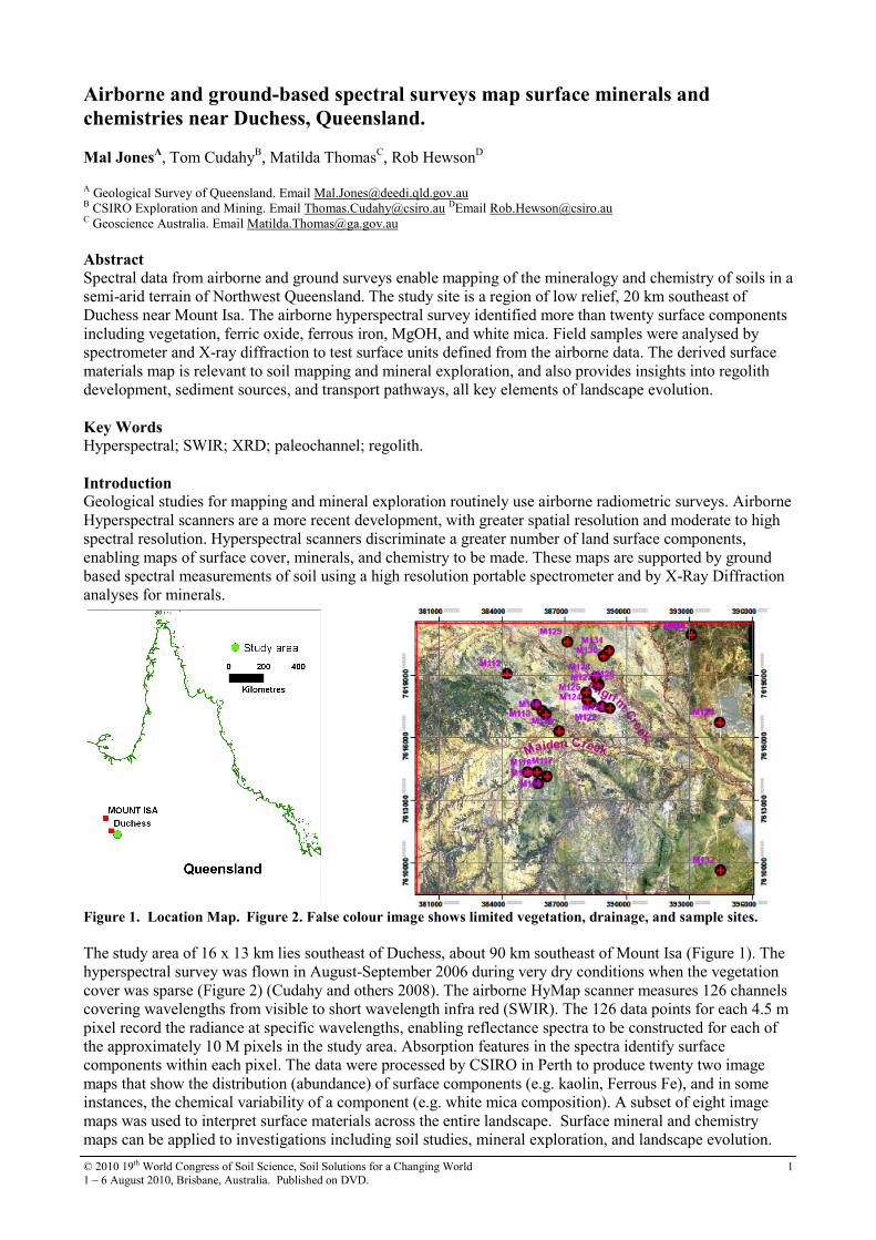
Figure 1. Location Map. Figure 2. False colour image shows limited vegetation, drainage, and sample sites.
The study area of 16 x 13 km lies southeast of Duchess, about 90 km southeast of Mount Isa (Figure 1). The
hyperspectral survey was flown in August-September 2006 during very dry conditions when the vegetation
cover was sparse (Figure 2) (Cudahy and others 2008). The airborne HyMap scanner measures 126 channels
covering wavelengths from visible to short wavelength infra red (SWIR). The 126 data points for each 4.5 m
pixel record the radiance at specific wavelengths, enabling reflectance spectra to be constructed for each of
the approximately 10 M pixels in the study area. Absorption features in the spectra identify surface
components within each pixel. The data were processed by CSIRO in Perth to produce twenty two image
maps that show the distribution (abundance) of surface components (e.g. kaolin, Ferrous Fe), and in some
instances, the chemical variability of a component (e.g. white mica composition). A subset of eight image
maps was used to interpret surface materials across the entire landscape. Surface mineral and chemistry
maps can be applied to investigations including soil studies, mineral exploration, and landscape evolution.
© 2010 19th World Congress of Soil Science, Soil Solutions for a Changing World
1 – 6 August 2010, Brisbane, Australia. Published on DVD. 2
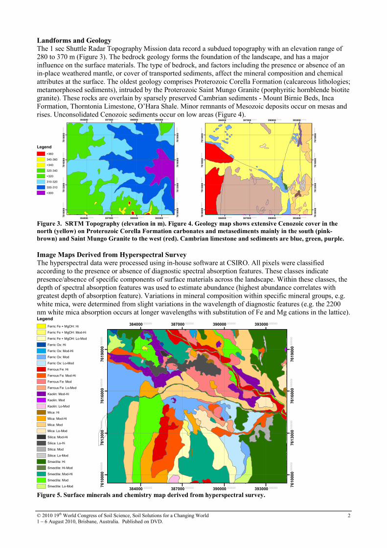
Landforms and Geology The 1 sec Shuttle Radar Topography Mission data record a subdued topography with an elevation range of
280 to 370 m (Figure 3). The bedrock geology forms the foundation of the landscape, and has a major
influence on the surface materials. The type of bedrock, and factors including the presence or absence of an
in-place weathered mantle, or cover of transported sediments, affect the mineral composition and chemical
attributes at the surface. The oldest geology comprises Proterozoic Corella Formation (calcareous lithologies;
metamorphosed sediments), intruded by the Proterozoic Saint Mungo Granite (porphyritic hornblende biotite
granite). These rocks are overlain by sparsely preserved Cambrian sediments - Mount Birnie Beds, Inca
Formation, Thorntonia Limestone, O’Hara Shale. Minor remnants of Mesozoic deposits occur on mesas and
rises. Unconsolidated Cenozoic sediments occur on low areas (Figure 4).
Legend
>360
340-360
>340
320-340
>320
310-320
300-310
<300
384000.000000
384000.000000
387000.000000
387000.000000
390000.000000
390000.000000
393000.000000
393000.000000
7610000
.00
00
00
7610000
.00
00
00
7613000
.00
00
00
7613000
.00
00
00
7616000
.00
00
00
7616000
.00
00
00
7619000
.00
00
00
7619000
.00
00
00
384000.000000
384000.000000
387000.000000
387000.000000
390000.000000
390000.000000
393000.000000
393000.000000
7610000
.00
00
00
7610000
.00
00
00
7613000
.000
000
7613000
.000
000
7616000
.00
00
00
7616000
.00
00
00
7619000
.00
00
00
7619000
.00
00
00
Figure 3. SRTM Topography (elevation in m). Figure 4. Geology map shows extensive Cenozoic cover in the
north (yellow) on Proterozoic Corella Formation carbonates and metasediments mainly in the south (pink-
brown) and Saint Mungo Granite to the west (red). Cambrian limestone and sediments are blue, green, purple.
Image Maps Derived from Hyperspectral Survey The hyperspectral data were processed using in-house software at CSIRO. All pixels were classified
according to the presence or absence of diagnostic spectral absorption features. These classes indicate
presence/absence of specific components of surface materials across the landscape. Within these classes, the
depth of spectral absorption features was used to estimate abundance (highest abundance correlates with
greatest depth of absorption feature). Variations in mineral composition within specific mineral groups, e.g.
white mica, were determined from slight variations in the wavelength of diagnostic features (e.g. the 2200
nm white mica absorption occurs at longer wavelengths with substitution of Fe and Mg cations in the lattice). Legend
Ferric Fe + MgOH: Hi
Ferric Fe + MgOH: Mod-Hi
Ferric Fe + MgOH: Lo-Mod
Ferric Ox: Hi
Ferric Ox: Mod-Hi
Ferric Ox: Mod
Ferric Ox: Lo-Mod
Ferrous Fe: Hi
Ferrous Fe: Mod-Hi
Ferrous Fe: Mod
Ferrous Fe: Lo-Mod
Kaolin: Mod-Hi
Kaolin: Mod
Kaolin: Lo-Mod
Mica: Hi
Mica: Mod-Hi
Mica: Mod
Mica: Lo-Mod
Silica: Mod-Hi
Silica: Lo-Hi
Silica: Mod
Silica: Lo-Mod
Smectite: Hi
Smectite: Hi-Mod
Smectite: Mod-Hi
Smectite: Mod
Smectite: Lo-Mod
384000.000000
384000.000000
387000.000000
387000.000000
390000.000000
390000.000000
393000.000000
393000.000000
7610000
.0000
00
7610000
.0000
00
7613000
.0000
00
7613000
.0000
00
7616000
.0000
00
7616000
.0000
00
7619000
.0000
00
7619000
.0000
00
Figure 5. Surface minerals and chemistry map derived from hyperspectral survey.
© 2010 19th World Congress of Soil Science, Soil Solutions for a Changing World
1 – 6 August 2010, Brisbane, Australia. Published on DVD. 3
Eight image maps were used to investigate the surface material characteristics: Aluminium Smectite; White
Mica; Kaolin; Ferrous Iron; Ferric Oxide; Ferric Fe and MgOH; Silica (Hydrated); and False Colour.
Polygons were constructed to depict areas of dominance or high abundance of components. Some areas rated
highly in a number of components, and could be assigned to more than one surface mineral class. Other
areas contained low abundances in all mineral and chemical groups (Figure 5).
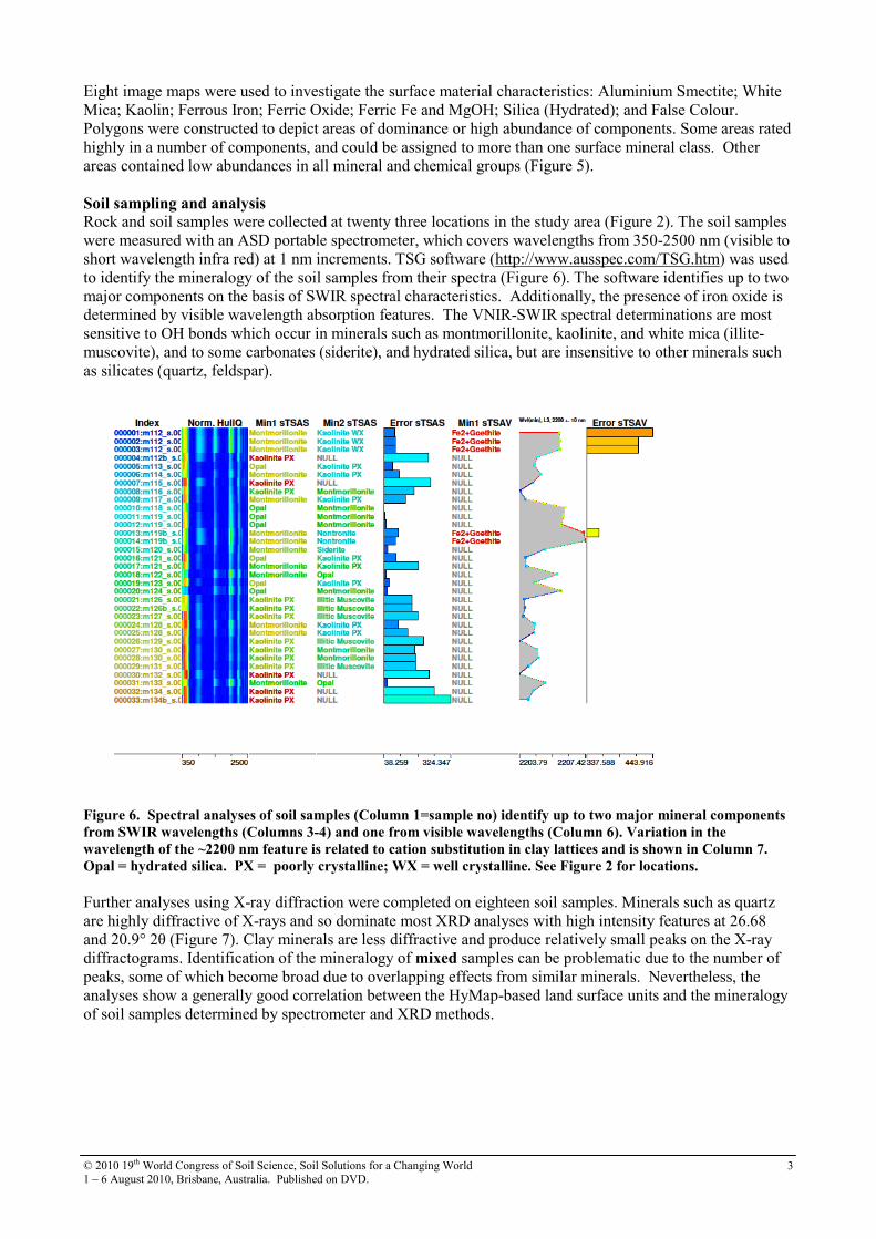
Soil sampling and analysis Rock and soil samples were collected at twenty three locations in the study area (Figure 2). The soil samples
were measured with an ASD portable spectrometer, which covers wavelengths from 350-2500 nm (visible to
short wavelength infra red) at 1 nm increments. TSG software (http://www.ausspec.com/TSG.htm) was used
to identify the mineralogy of the soil samples from their spectra (Figure 6). The software identifies up to two
major components on the basis of SWIR spectral characteristics. Additionally, the presence of iron oxide is
determined by visible wavelength absorption features. The VNIR-SWIR spectral determinations are most
sensitive to OH bonds which occur in minerals such as montmorillonite, kaolinite, and white mica (illite-
muscovite), and to some carbonates (siderite), and hydrated silica, but are insensitive to other minerals such
as silicates (quartz, feldspar).
Figure 6. Spectral analyses of soil samples (Column 1=sample no) identify up to two major mineral components
from SWIR wavelengths (Columns 3-4) and one from visible wavelengths (Column 6). Variation in the
wavelength of the ~2200 nm feature is related to cation substitution in clay lattices and is shown in Column 7.
Opal = hydrated silica. PX = poorly crystalline; WX = well crystalline. See Figure 2 for locations.
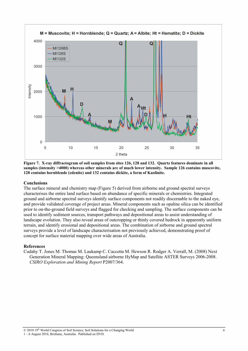
Further analyses using X-ray diffraction were completed on eighteen soil samples. Minerals such as quartz
are highly diffractive of X-rays and so dominate most XRD analyses with high intensity features at 26.68
and 20.9° 2θ (Figure 7). Clay minerals are less diffractive and produce relatively small peaks on the X-ray
diffractograms. Identification of the mineralogy of mixed samples can be problematic due to the number of
peaks, some of which become broad due to overlapping effects from similar minerals. Nevertheless, the
analyses show a generally good correlation between the HyMap-based land surface units and the mineralogy
of soil samples determined by spectrometer and XRD methods.
© 2010 19th World Congress of Soil Science, Soil Solutions for a Changing World
1 – 6 August 2010, Brisbane, Australia. Published on DVD. 4
0
1000
2000
3000
4000
5 10 15 20 25 30 35
2 theta
Inte
nsity
MI126BS
MI128S
MI132S
M
M
H
HA
D
D
A
AHt
Ht
Q Q
M = Muscovite; H = Hornblende; Q = Quartz; A = Albite; Ht = Hematite; D = Dickite
Figure 7. X-ray diffractogram of soil samples from sites 126, 128 and 132. Quartz features dominate in all
samples (intensity >4000) whereas other minerals are of much lower intensity. Sample 126 contains muscovite,
128 contains hornblende (edenite) and 132 contains dickite, a form of Kaolinite.
Conclusions The surface mineral and chemistry map (Figure 5) derived from airborne and ground spectral surveys
characterises the entire land surface based on abundance of specific minerals or chemistries. Integrated
ground and airborne spectral surveys identify surface components not readily discernable to the naked eye,
and provide validated coverage of project areas. Mineral components such as opaline silica can be identified
prior to on-the-ground field surveys and flagged for checking and sampling. The surface components can be
used to identify sediment sources, transport pathways and depositional areas to assist understanding of
landscape evolution. They also reveal areas of outcropping or thinly covered bedrock in apparently uniform
terrain, and identify erosional and depositional areas. The combination of airborne and ground spectral
surveys provide a level of landscape characterisation not previously achieved, demonstrating proof of
concept for surface material mapping over wide areas of Australia.
References Cudahy T. Jones M. Thomas M. Laukamp C. Caccetta M. Hewson R. Rodger A. Verrall, M. (2008) Next
Generation Mineral Mapping: Queensland airborne HyMap and Satellite ASTER Surveys 2006-2008.
CSIRO Exploration and Mining Report P2007/364.

© 2010 19th World Congress of Soil Science, Soil Solutions for a Changing World
1 – 6 August 2010, Brisbane, Australia. Published on DVD. 5
An assessment of diffuse reflectance mid-infrared spectroscopy for measuring
soil carbon, nitrogen and microbial biomass
Dinesh Babu MadhavanAH
, Daniel MendhamBH
, Pauline MeleC, Sabine Kasel
D, Matt Kitching
E,
Christopher WestonFH
and Thomas BakerGH
ADepartment of Forest and Ecosystem Science, The University of Melbourne, Burnley, VIC 3121, Australia,
Email [email protected] BCSIRO Sustainable Ecosystems, Wembley, WA 6913, Australia, Email [email protected] CDepartment of Primary Industries, Knoxfield 3180, VIC, Australia, Email [email protected] DDepartment of Forest and Ecosystem Science, The University of Melbourne, Burnley 3121, VIC, Australia,
Email [email protected] EDepartment of Primary Industries, Werribee, VIC 3030, Australia, Email [email protected] FDepartment of Forest and Ecosystem Science, The University of Melbourne, Creswick, VIC 3363, Australia,
Email [email protected] GDepartment of Forest and Ecosystem Science, The University of Melbourne, Burnley, VIC 3121, Australia,
Email [email protected] HCooperative Research Centre for Forestry, Australia, www.crcforestry.com.au
Abstract Surface soils from three land-use and land-use change studies in southern Australia were used to explore
mid-infrared spectroscopy (MIRS) coupled with partial least squares regression (PLSR) to measure soil
total C, total N and microbial biomass carbon (MBC). The soils were from agriculture (crop and pasture),
forest plantation, and native vegetation land-uses. Prediction on the validation set for total C and total N
(R2 = 0.94 and 0.86) were excellent, and that for MBC (R
2 = 0.53) was fair. The methodology has sufficient
accuracy across a range of soils for application to determine the effects of land-use on these key indicator
soil properties.
Key Words Mid-infrared reflectance spectroscopy, soil, carbon, nitrogen, microbial biomass.
Introduction Soil organic matter is heterogeneous with a wide range of functional types having variable turnover rates and
nutrient release potential. Land-use and land-use change can affect the quantity and quality of soil organic
matter, thus affecting soil properties and plant growth. For example, trees planted on land previously
managed for agriculture (usually pastures) in southern Australia have benefited from the relatively high soil
fertility arising from past fertiliser application and N-fixation by legumes. However, declines in N-availability
over a rotation have been observed (e.g., O’Connell et al. 2003), and a challenge for plantation managers is
to better understand such changes so as to maintain and build soil fertility.
Mid infrared reflectance spectroscopy (MIRS) has been demonstrated to be useful for the analysis of soils,
including for total and various fractions of carbon, some nutrients, and soil texture (e.g., Janik et al. 2007,
Viscarra Rossel et al. 2006). Once calibrated, it can be a cost-effective and rapid technique to assess soil
fertility and health indices (e.g., Viscarra Rossel et al. 2008)
The work reported here draws on previous studies from a wide range of land-uses, soil textures and annual
rainfall in southern Australia to assess the accuracy of MIRS to predict soil total C, total N and microbial
biomass carbon (MBC).
Methods Sites and sampling
Soils from three land-use / land-use change comparison studies were analysed:
• Pasture – Eucalyptus globulus plantation: Thirty one paired sites in south-western Western Australia, 0–
10 cm depth, 4 replicates per site (n = 248) (O’Connell et al. 2003). Plantations were established on
long-term pastures, and were sampled during late winter to early spring in the first rotation at 6 to 11
years of age.
© 2010 19th World Congress of Soil Science, Soil Solutions for a Changing World
1 – 6 August 2010, Brisbane, Australia. Published on DVD. 6
• Crop – Remnant vegetation: Thirty paired sites in north-eastern, north-western and south-western
Victoria, 0–10 cm depth, 6 replicates per site (n = 360) (Mele and Crowley 2008). The remnant
vegetation included land under native vegetation, whereas the cropped soils had been managed
conventionally for cereal, legume, vegetable, citrus and grape production.
• Pinus radiata plantation – Native forest (mixed Eucalyptus spp.): Eleven site-types across north-eastern
Victoria and south-eastern NSW (3 or 4 sample plots per site-type), 0 – 5 and 5 – 10 cm depth, 3
replicates per plot (n = 204) (Kasel and Bennett 2007). The study comprised pine plantations in their first
and second rotations (ex-native forest, ex-pasture), regenerated woodlands (ex-pasture, mixed eucalypt)
and rehabilitated forest (ex-pine plantation, ex-pasture), and sampled during late spring and late autumn.
The three studies (n = 812) represented a wide range of soil textures (sandy to clay loam) and climate (mean
annual rainfall 776 to 1400 mm). Each soil sample analysed was a composite of 6 to 9 cores.
Soil total C, total N and microbial biomass carbon
Total soil C and N were determined on finely ground (< 0.5 mm) and oven-dried (40oC) subsamples using a
Leco CN analyser. Microbial biomass carbon (MBC) was measured on rewetted and incubated soil
subsamples (< 2 mm) by the fumigation extraction method (Sparling and West 1988), using an extraction
factor (kEC, 0.3 to 0.38) to convert the oxidisable organic-C flush to microbial-C, based on soil textures
(Vance et al. 1987; Inubushi et al. 1991).
MIRS
Air-dried soil subsamples (< 2 mm) were finely ground in a vibrating puck mill for one minute. Mid-infrared
diffuse reflectance spectra for these soils were collected using a PerkinElmer Spectrum One FT-IR
spectrometer from 7800 to 450 /cm at 8 /cm resolution. Scans were co-added for one minute. A reference
background spectrum was recorded at the start and after every thirty minutes or every 15 samples, whichever
occurred sooner.
PLSR
Matlab (version 7.8.0.347) and PLS_Toolbox 4.2 were used to fit partial least squares regression (PLSR)
calibration with leave-one-out cross-validations. Data were first transformed using a cube root (total C),
square root (total N) or fourth root (MBC) to normalise the distributions. Spectra were preprocessed using
multiplicative scatter correction (MSC-mean) followed by first derivative and auto scaling. One-third of the
data, representing all land-uses, was randomly selected to form a validation subset and the rest used for the
calibration subset.
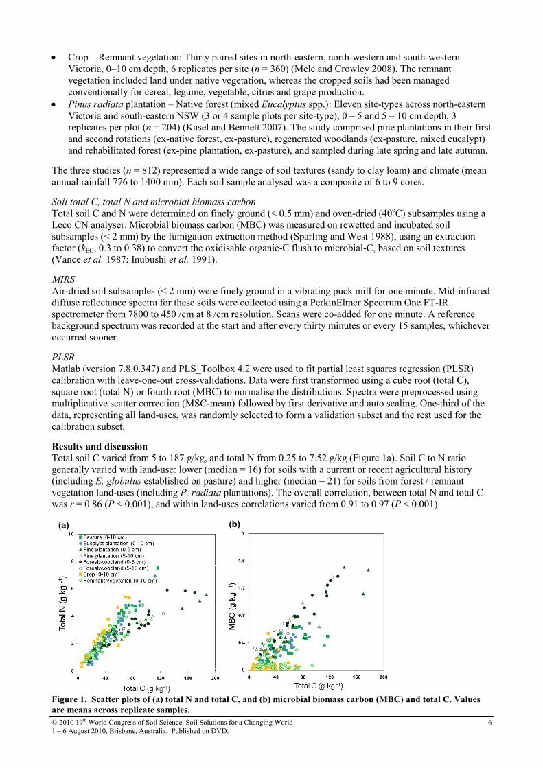
Results and discussion Total soil C varied from 5 to 187 g/kg, and total N from 0.25 to 7.52 g/kg (Figure 1a). Soil C to N ratio
generally varied with land-use: lower (median = 16) for soils with a current or recent agricultural history
(including E. globulus established on pasture) and higher (median = 21) for soils from forest / remnant
vegetation land-uses (including P. radiata plantations). The overall correlation, between total N and total C
was r = 0.86 (P < 0.001), and within land-uses correlations varied from 0.91 to 0.97 (P < 0.001).
(a) (b)
Figure 1. Scatter plots of (a) total N and total C, and (b) microbial biomass carbon (MBC) and total C. Values
are means across replicate samples.
© 2010 19th World Congress of Soil Science, Soil Solutions for a Changing World
1 – 6 August 2010, Brisbane, Australia. Published on DVD. 7
Soil MBC varied from 0.01 to 1.51 g/kg and was broadly correlated with total C (r = 0.76, P < 0.001,
Figure 1b). Within land-uses, the correlation for cropped soils, generally having the lowest MBC values, was
not significant, whereas correlations for other land-uses were significant (r = 0.72 to 0.96, P < 0.001).
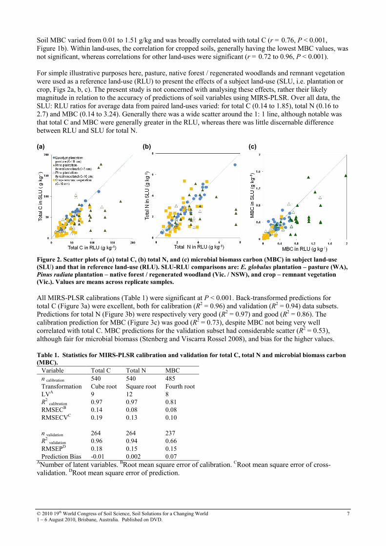
For simple illustrative purposes here, pasture, native forest / regenerated woodlands and remnant vegetation
were used as a reference land-use (RLU) to present the effects of a subject land-use (SLU, i.e. plantation or
crop, Figs 2a, b, c). The present study is not concerned with analysing these effects, rather their likely
magnitude in relation to the accuracy of predictions of soil variables using MIRS-PLSR. Over all data, the
SLU: RLU ratios for average data from paired land-uses varied: for total C (0.14 to 1.85), total N (0.16 to
2.7) and MBC (0.14 to 3.24). Generally there was a wide scatter around the 1: 1 line, although notable was
that total C and MBC were generally greater in the RLU, whereas there was little discernable difference
between RLU and SLU for total N.
(a)
(b)
(c)
Figure 2. Scatter plots of (a) total C, (b) total N, and (c) microbial biomass carbon (MBC) in subject land-use
(SLU) and that in reference land-use (RLU). SLU-RLU comparisons are: E. globulus plantation – pasture (WA),
Pinus radiata plantation – native forest / regenerated woodland (Vic. / NSW), and crop – remnant vegetation
(Vic.). Values are means across replicate samples.
All MIRS-PLSR calibrations (Table 1) were significant at P < 0.001. Back-transformed predictions for
total C (Figure 3a) were excellent, both for calibration (R2 = 0.96) and validation (R
2 = 0.94) data subsets.
Predictions for total N (Figure 3b) were respectively very good (R2 = 0.97) and good (R
2 = 0.86). The
calibration prediction for MBC (Figure 3c) was good (R2 = 0.73), despite MBC not being very well
correlated with total C. MBC predictions for the validation subset had considerable scatter (R2 = 0.53),
although fair for microbial biomass (Stenberg and Viscarra Rossel 2008), and bias for the higher values.
Table 1. Statistics for MIRS-PLSR calibration and validation for total C, total N and microbial biomass carbon
(MBC).
Variable Total C Total N MBC
n calibration 540 540 485
Transformation Cube root Square root Fourth root
LVA 9 12 8
R2 calibration 0.97 0.97 0.81
RMSECB 0.14 0.08 0.08
RMSECVC 0.19 0.13 0.10
n validation 264 264 237
R2 validation 0.96 0.94 0.66
RMSEPD 0.18 0.15 0.15
Prediction Bias -0.01 0.002 0.07 ANumber of latent variables.
BRoot mean square error of calibration.
CRoot mean square error of cross-
validation. DRoot mean square error of prediction.
© 2010 19th World Congress of Soil Science, Soil Solutions for a Changing World
1 – 6 August 2010, Brisbane, Australia. Published on DVD. 8
(a)
(b)
(c)
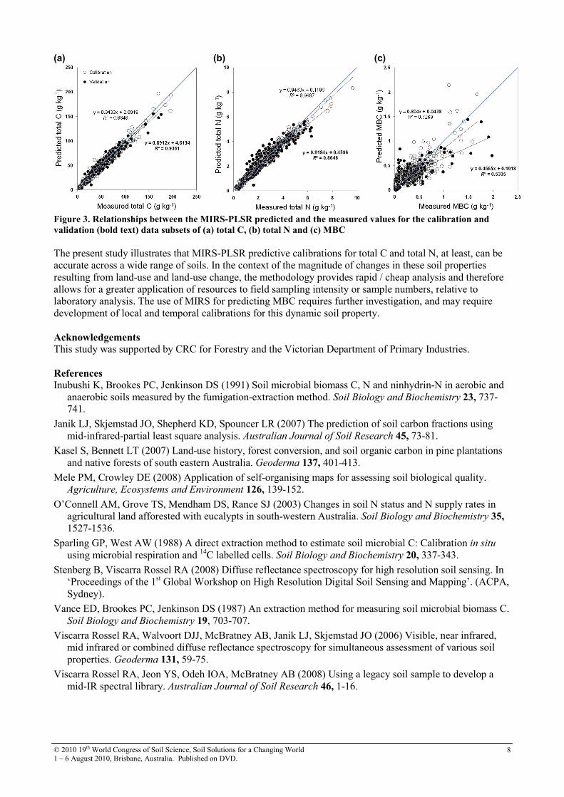
Figure 3. Relationships between the MIRS-PLSR predicted and the measured values for the calibration and
validation (bold text) data subsets of (a) total C, (b) total N and (c) MBC
The present study illustrates that MIRS-PLSR predictive calibrations for total C and total N, at least, can be
accurate across a wide range of soils. In the context of the magnitude of changes in these soil properties
resulting from land-use and land-use change, the methodology provides rapid / cheap analysis and therefore
allows for a greater application of resources to field sampling intensity or sample numbers, relative to
laboratory analysis. The use of MIRS for predicting MBC requires further investigation, and may require
development of local and temporal calibrations for this dynamic soil property.
Acknowledgements This study was supported by CRC for Forestry and the Victorian Department of Primary Industries.
References Inubushi K, Brookes PC, Jenkinson DS (1991) Soil microbial biomass C, N and ninhydrin-N in aerobic and
anaerobic soils measured by the fumigation-extraction method. Soil Biology and Biochemistry 23, 737-
741.
Janik LJ, Skjemstad JO, Shepherd KD, Spouncer LR (2007) The prediction of soil carbon fractions using
mid-infrared-partial least square analysis. Australian Journal of Soil Research 45, 73-81.
Kasel S, Bennett LT (2007) Land-use history, forest conversion, and soil organic carbon in pine plantations
and native forests of south eastern Australia. Geoderma 137, 401-413.
Mele PM, Crowley DE (2008) Application of self-organising maps for assessing soil biological quality.
Agriculture, Ecosystems and Environment 126, 139-152.
O’Connell AM, Grove TS, Mendham DS, Rance SJ (2003) Changes in soil N status and N supply rates in
agricultural land afforested with eucalypts in south-western Australia. Soil Biology and Biochemistry 35,
1527-1536.
Sparling GP, West AW (1988) A direct extraction method to estimate soil microbial C: Calibration in situ
using microbial respiration and 14
C labelled cells. Soil Biology and Biochemistry 20, 337-343.
Stenberg B, Viscarra Rossel RA (2008) Diffuse reflectance spectroscopy for high resolution soil sensing. In
‘Proceedings of the 1st Global Workshop on High Resolution Digital Soil Sensing and Mapping’. (ACPA,
Sydney).
Vance ED, Brookes PC, Jenkinson DS (1987) An extraction method for measuring soil microbial biomass C.
Soil Biology and Biochemistry 19, 703-707.
Viscarra Rossel RA, Walvoort DJJ, McBratney AB, Janik LJ, Skjemstad JO (2006) Visible, near infrared,
mid infrared or combined diffuse reflectance spectroscopy for simultaneous assessment of various soil
properties. Geoderma 131, 59-75.
Viscarra Rossel RA, Jeon YS, Odeh IOA, McBratney AB (2008) Using a legacy soil sample to develop a
mid-IR spectral library. Australian Journal of Soil Research 46, 1-16.
© 2010 19th World Congress of Soil Science, Soil Solutions for a Changing World
1 – 6 August 2010, Brisbane, Australia. Published on DVD. 9
An automated system for rapid in-field soil nutrient testing
Craig LobseyA, Raphael Viscarra Rossel
B and Alex McBratney
A
AAustralian Centre for Precision Agriculture, University of Sydney, Sydney, Australia, Email [email protected]
BCSIRO Land & Water, Canberra, Australia
Abstract This paper outlines the laboratory experimentation and development of a multi-ion measuring system
(MIMS) for proximal sensing of soil nitrate, potassium and sodium using Ion Selective Electrodes (ISEs).
We present work conducted for characterising ion exchange reactions using multiple ISEs and a universal
extracting solution. The use of ion exchange kinetics and prediction models for rapid estimation of soil
extractable nutrient concentration was evaluated. Using these techniques the prototype laboratory and field
portable MIMS was developed to provide rapid in-field soil nutrient analysis in less than 30 seconds. The
system automates the measurement process including ISE calibration, temperature compensation, and soil
analysis with nutrient estimation. Finally we describe the hardware and the performance of the MIMS under
laboratory and field conditions.
Key Words Proximal soil sensing, Ion Selective Electrodes (ISE), ion exchange kinetics, precision agriculture.
Introduction The implementation of Precision Agriculture (PA) is important for optimising crop production and economic
return to farmers, and reducing the environmental impact of farming operations. More precise and accurate
resource application (e.g. fertiliser, lime, etc) both spatially and temporally may reduce their over or under
application, thereby ensuring optimum productivity for any given unit of land. This management philosophy
requires the collection of high resolution soil chemical and physical information, which can not be met by
conventional sampling and laboratory analysis. The reason is the large labor requirements, the expense and
time needed, making conventional methods inefficient (Viscarra Rossel & Walter 2004). For this reason the
development of Proximal Soil Sensors (PSS) is important. These sensors should be rapid, inexpensive, robust
and capable of repeatable measurements. A number of proximal soil sensors have been developed and are
commercially available. For example electromagnetic induction (EMI) instruments (Sudduth et al. 2001),
electrical conductivity systems (e.g. Lund et al. 1999) and a pH sensor (Adamchuk et al. 1999). Currently,
there are no commercially available proximal soil sensors that measure soil nutrient concentration directly.
Our sensor is novel in that it aims to bridge the gap between conventional sampling and analysis and current
proximal soil sensors by providing direct chemical measurements of soil nutrients at intermediate
resolutions. We developed the system with the view that it should be versatile enough to be used as:
1) A field portable sensor for site specific nutrient analysis, soil core analysis, or screening of critical
nutrient concentrations.
2) The analytical unit for an automated on-the-go sampling system for high resolution mapping of
soil nitrate, sodium and potassium
The first will provide rapid, low cost analysis of nutrient concentrations through the soil profile, for example,
allowing a larger number of soil cores to be analyzed in the field and minimising the need for returning
samples to the laboratory. The second will provide information on the spatial variability of soil nutrient
concentrations within approximately the top 20 cm of the soil profile.
Ion Selective Electrodes for soil nutrient sensing Ion Selective Electrodes (ISEs) are capable of providing direct measurements in unfiltered soil extract or
slurries, making them attractive options for proximal soil sensing. They are small, economical and require
little supporting hardware. Proximal sensing of soil pH using ISEs has been demonstrated by (Adamchuk et
al. 1999) and commercially available (Veris pH manager – Veris Technologies). Initial techniques
employing ISE technology such as Direct Soil Sampling (DSM) for measurement of K+, Na
+ and NO3
- on
naturally moist soil samples (Adamchuk et al. 2005) have experienced limited success. These studies
demonstrate the applicability of ISEs for proximal soil nutrient sensing, however the rather rudimentary
techniques used to make the measurements and the consequent inconsistencies in the measurements are their
major drawback and accountable for their limited success.
Previous work has also inherently been limited to soluble or plant available ion concentrations. Information
© 2010 19th World Congress of Soil Science, Soil Solutions for a Changing World
1 – 6 August 2010, Brisbane, Australia. Published on DVD. 10
on both soluble and exchangeable components is important in management decisions due to the buffering
nature of the soil, for example in the measurement of lime requirement (LR) and fertilizer application.
However, this requires a lengthy soil extract procedure which creates the rate limiting component of the
measurement process.
Ion Exchange Kinetics – Observation and steady state prediction To overcome the rate limiting ion exchange processes it is proposed that the observation of the ion exchange
kinetics on addition of soil to the extracting solution will yield sufficient information to predict the steady
state or equilibrium concentration. Conceptually, this work continues from that of Viscarra Rossel and
McBratney (2003) and Viscarra Rossel et al. (2005) where the monitoring of the kinetics of pH reactions in a
batch system was used to estimate LR in a prototype on-the-go proximal sensor.
A series of half-cell ISEs selective for nitrate, sodium and potassium using a shared lithium acetate double
junction reference electrode were used in a batch processing system for the real-time monitoring of initial ion
exchange kinetics. To improve extraction rates and sensor performance an extracting solution of 0.1M
Magnesium Sulphate was chosen. Choices were limited by ISE interferences and selectivity.
Solution Phase [NO3-]
0
2
4
6
8
10
12
14
5 15 25
Time (s)
Nitrate (ppm)
Solution Phase [Na+]
0
5
10
15
20
25
5 15 25
Time (s)
Sodium (ppm)
Solution Phase [K+]
0
10
20
30
40
50
60
5 15 25
Time (s)
Potassium (ppm)
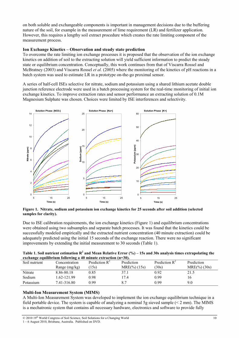
Figure 1. Nitrate, sodium and potassium ion exchange kinetics for 25 seconds after soil addition (selected
samples for clarity).
Due to ISE calibration requirements, the ion exchange kinetics (Figure 1) and equilibrium concentrations
were obtained using two subsamples and separate batch processes. It was found that the kinetics could be
successfully modeled empirically and the extracted nutrient concentration (40 minute extraction) could be
adequately predicted using the initial 15 seconds of the exchange reaction. There were no significant
improvements by extending the initial measurement to 30 seconds (Table 1).
Table 1. Soil nutrient estimation R
2 and Mean Relative Error (%) – 15s and 30s analysis times extrapolating the
exchange equilibrium following a 40 minute extraction (n=30). Soil nutrient Concentration
Range (mg/kg)
Prediction R2
(15s)
Prediction
MRE(%) (15s)
Prediction R2
(30s)
Prediction
MRE(%) (30s)
Nitrate 8.86-80.18 0.85 37.1 0.92 21.5
Sodium 1.62-121.99 0.98 17.4 0.99 16
Potassium 7.41-316.80 0.99 8.7 0.99 9.0
Multi-Ion Measurement System (MIMS) A Multi-Ion Measurement System was developed to implement the ion exchange equilibrium technique in a
field portable device. The system is capable of analyzing a nominal 5g sieved sample (< 2 mm). The MIMS
is a mechatronic system that contains all necessary hardware, electronics and software to provide fully
© 2010 19th World Congress of Soil Science, Soil Solutions for a Changing World
1 – 6 August 2010, Brisbane, Australia. Published on DVD. 11
autonomous sample analysis including reagent injection, agitation, kinetics monitoring and soil nutrient
predictions (Figure 2 and Figure 3). ISE calibration is also performed automatically and includes ‘quality’
control of the ISEs.
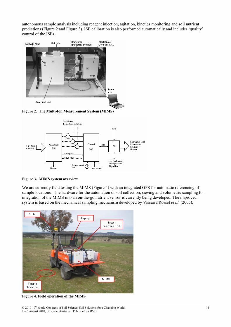
Figure 2. The Multi-Ion Measurement System (MIMS)
Figure 3. MIMS system overview
We are currently field testing the MIMS (Figure 4) with an integrated GPS for automatic referencing of
sample locations. The hardware for the automation of soil collection, sieving and volumetric sampling for
integration of the MIMS into an on-the-go nutrient sensor is currently being developed. The improved
system is based on the mechanical sampling mechanism developed by Viscarra Rossel et al. (2005).
Figure 4. Field operation of the MIMS

© 2010 19th World Congress of Soil Science, Soil Solutions for a Changing World
1 – 6 August 2010, Brisbane, Australia. Published on DVD. 12
Conclusion The MIMS system was developed to automate the analytical components of soil nutrient testing with the
goal of providing: (i) a field portable system for simple and rapid estimation of soil nutrient concentrations
through the soil profile and (ii) to characterize the spatial variability of nutrient concentrations in surface soil.
In both these roles this sensor will provide an improved understanding of soil nutrient variability both
spatially and temporally. It will provide sensing capabilities for more effective continuous and site specific
nutrient management.
Acknowledgements This work is being funded by the Grains Research and Development Corporation (GRDC).
References Adamchuk VI, Lund ED, Sethuramasamyraja B, Morgan MT, Dobermann A, Marx DB (2005) Direct
measurement of soil chemical properties on-the-go using ion-selective electrodes. Computers and
Electronics in Agriculture 48, 272-294.
Adamchuk VI, Morgan MT, Ess DR (1999) An automated sampling system for measuring soil pH.
Transactions of the Asae 42, 885-891.
Lund ED, Colin PE, Christy D, Drummond PE (1999) Applying soil electrical conductivity technology to
precision agriculture. In ‘Precision Agriculture:Proc. Int. Conf., 4th, St. Paul, MN. 19-22 July 1998’.
(Eds PC Robert et al.). (ASA, CSSA, and SSA, Madison, WI.)
Sudduth KA, Drummond ST, Kitchen NR (2001) Accuracy issues in electromagnetic induction sensing of
soil electrical conductivity for precision agriculture. Computers and Electronics in Agriculture 31,
239-264.
Viscarra Rossel RA, Gilbertson M, Thylen L, Hansen O, McVey S, McBratney AB (2005) Field
measurements of soil pH and lime requirement using an on-the-go soil pH and lime requirement
measurement system. In 'Precision agriculture '05. Papers presented at the 5th European Conference
on Precision Agriculture, Uppsala, Sweden.' pp. 511-520.
Viscarra Rossel RA, McBratney AB (2003) Modelling the kinetics of buffer reactions for rapid field
predictions of lime requirements. Geoderma 114, 49-63.
Viscarra Rossel RA, Walter C (2004) Rapid, quantitative and spatial field measurements of soil pH using an
Ion Sensitive Field Effect Transistor. Geoderma 119, 9-20.
© 2010 19th World Congress of Soil Science, Soil Solutions for a Changing World
1 – 6 August 2010, Brisbane, Australia. Published on DVD. 13
An infrared spectroscopic test for total petroleum hydrocarbon (TPH)
contamination in soils
Sean ForresterA,B
, Les JanikA and Mike McLaughlin
A
ACSIRO Land and Water BCorresponding author. Email [email protected]
Abstract The application of near- and mid-infrared (NIR and MIR) spectroscopy as a rapid screening tool for TPH
concentrations in contaminated soils is presented. MIR-DRIFT (diffuse reflectance infrared Fourier-
transform) spectroscopy, in particular, promises to be a revolutionary new technique for the in-situ analysis
of soils at contaminated sites. Infrared is sensitive to alkyl vibrational frequencies, allowing the use of
partial least squares (PLS) to be used for quantification of TPH. This work showed that neat whole soils
could be used, spectra can be acquired rapidly, and MIR TPH spectra could be separated from those of
natural soil organic matter. PLS regression analyses were carried out in three stages; spiking diesel and
crude oil (as TPH) into reference minerals, spiking into reference soils, and actual TPH concentrations in
contaminated soils. Results of PLS cross-validation for the spiked minerals showed that prediction errors
(RMSECV) with the MIR DRIFT were approximately 2000-4000 mg/kg for a TPH range of 0-100,000
mg/kg, but slightly higher for the NIR. (4500-8000 mg/kg). RMSECV values for the reference soils were
approximately 1500-2500 mg/kg for a 0-25,000 mg/kg TPH range. Tests with actual contaminated soils
identified specific peaks in the MIR that were characteristic of TPH, and showed that predictions using these
peaks resulted in RMSECV of approximately 4,500 mg/kg for a 0-60,000 mg/kg TPH range and thus
suitable for use as a screening tool.
Key Words TPH, PLS, infrared, soils, DRIFT.
Introduction Currently, most soil analyses for TPH use a gas-chromatographic (GC) based laboratory method for
determining TPH concentration. Although this method is the industry standard, as required by state
regulatory agencies, it is time-consuming, requires a NATA accredited laboratory, and is not suited to field-
portable or on-site applications. A more simple and rapid alternative method for screening contaminated
sites for TPH would be desirable, even if slightly less accurate, for initial TPH screening of samples at
contaminated sites.
Infrared (IR) techniques may satisfy these requirements, particularly with the availability of portable
spectrometers. A literature search resulted in very few studies on the use of IR for TPH determination in
soils, and in particular using unprocessed neat whole soils (Malley et al. 1999). Currently, a quantitative
assessment of TPH can be carried out with an ATR (attenuated total reflection) infrared technique following
solvent extraction of TPH from the soil sample. However, the extraction method is somewhat tedious to
carry out in the field and, due to the extraction step, is not rapid nor lends itself to in-field application as a
direct measurement method. This work outlines the scientific basis, methodologies and the results for the
prediction of TPH concentrations in contaminated soils using Fourier transform infrared (FTIR) spectroscopy
and partial least squares (PLS) regression on neat whole soils. The results demonstrate the potential of mid-
infrared DRIFT spectroscopy for TPH using laboratory based and field portable spectrometers.
Near-infrared (NIR) and mid-infrared (MIR) spectra are sensitive to alkyl functional chemical groups in
organic materials, including TPH compounds. These techniques therefore have the possibility of screening
contaminated soils to determine TPH contamination. An advantage of IR methods is that un-processed neat,
whole soil samples can be studied by diffuse reflectance infrared (DRIFT) spectroscopy, where the samples
are simply put under an incoming infrared beam and the reflected signal analysed. However, there are
inherent problems with the application of the DRIFT technique to whole soil analysis of TPH. The first
problem is the overlap of TPH-sensitive infrared peaks with those of naturally occurring soil organic matter
(SOM), so that identification of spectral peaks unique to TPH is difficult. Adding to this problem is masking
of many of the TPH peaks in the MIR in spectral regions dominated by quartz and other soil mineral spectra.
© 2010 19th World Congress of Soil Science, Soil Solutions for a Changing World
1 – 6 August 2010, Brisbane, Australia. Published on DVD. 14
A second known problem with infrared reflectance is the shielding to IR radiation to the internal structure of
soil micro-aggregates. This study attempts to address some of these problems and develop a rapid in-situ
screening technique for TPH contamination of soils.
The project was carried out in three stages. The first stage dealt with the sorption of diesel and crude oil
(representing TPH) into some common soil clay minerals (illite, smectite, kaolinite), sand, mixtures of clay
and sand, and a range of quartz particle sizes. The second and third stages focused on TPH sorption into two
standard reference soils, and on a wider range of field soils from actual TPH contaminated sites. Various
spectrometer options, including dispersive and FTIR instrumentation, were available for alternative NIR and
MIR spectral ranges and sample presentations. It was thus hoped to demonstrate that infrared spectroscopy
could be used to speed up routine TPH analysis, allowing for more timely management decisions to be made
with regard to site contamination and remediation, with a potential for future in-field or on-site application.
Methods Samples
Crude oil and diesel at various concentrations were spiked into reference soil minerals and soils and analysed
using FTIR and NIR reflectance with PLS regression. Minerals used were sand, bentonite, kaolinite, illite
and limestone. Stock solutions of TPH were prepared from crude oil and diesel dissolved in cyclohexane.
The aliquots were mixed with fixed weights of each sample in a tumbler to ensure an even dispersion of TPH
throughout the sample particles and then the samples were dried to remove the cyclohexane. Loss of TPH
resulted in only 2% in 24 hrs. Two sets of “real” contaminated soils were tested; set “S” consisting of 34
soils and set “L” consisting of 138 samples. Most of the TPH as analysed by the primary laboratory method
was found in the C15-C28 carbon length fraction.
Spectroscopy
MIR DRIFT spectra were scanned using approximately 100 mg of soil with a Perkin-Elmer Spectrum-One
Fourier transform mid-infrared (FTIR) spectrometer (Perkin Elmer Inc., Mass. USA). Spectra were scanned
for 60 seconds in the frequency (wavenumber) range 7800 to 450 /cm (wavelength range 1280 to 22000 nm)
at a resolution of 8 /cm. Reference scans of liquid crude oil and diesel were also obtained by two reflectance
methods; as films deposited directly onto a mirror surface (transflectance) and dispersed on the surface of
powdered KBr (DRIFT). NIR spectra were scanned using a FOSS NIRSystems 6500 Vis-NIR spectrometer
(Foss NIRSystems, Silver Springs, MD, USA) with a wavelength range of 400 – 2500 nm. Samples for NIR
were placed “as received” into a quartz macro-sampling cuvette with an area of approximately 200x25 mm
and scanned in reflectance mode. Reference scans of crude oil and diesel were carried out by transmittance
using a 1 mm quartz cuvette. Portable NIR and MIR spectrometers were also tested.
PLS chemometrics
Spectra were processed with the Unscrambler Ver. 9.60 software (CAMO technologies, Inc, 152
Woodbridge, NJ). Principal components analysis (PCA) and PLS calibrations were carried out using full
"leave-one-out" cross-validation (Geladi and Kowalski 1986). Cross-validation regression statistics were
expressed in terms of the coefficient of determination (R2) and root mean square error of cross-validation
(RMSECV). The detection limit was taken as 2.0 x RMSECV.
Results and discussion Peaks characteristic of alkyl–CH3 and –CH2 stretching vibrations were observed in the ranges 4500-4200 /cm
and 3000-2700 /cm. Of the various alkyl absorbance peaks, one was observed and attributed to the first
overtone vibration of the –CH3 symmetric deformation mode in TPH but this peak was not observed in the
spectra of soil organic matter SOM. These seemed to be related to the amount of diesel in the spiked
samples rather than to SOM.
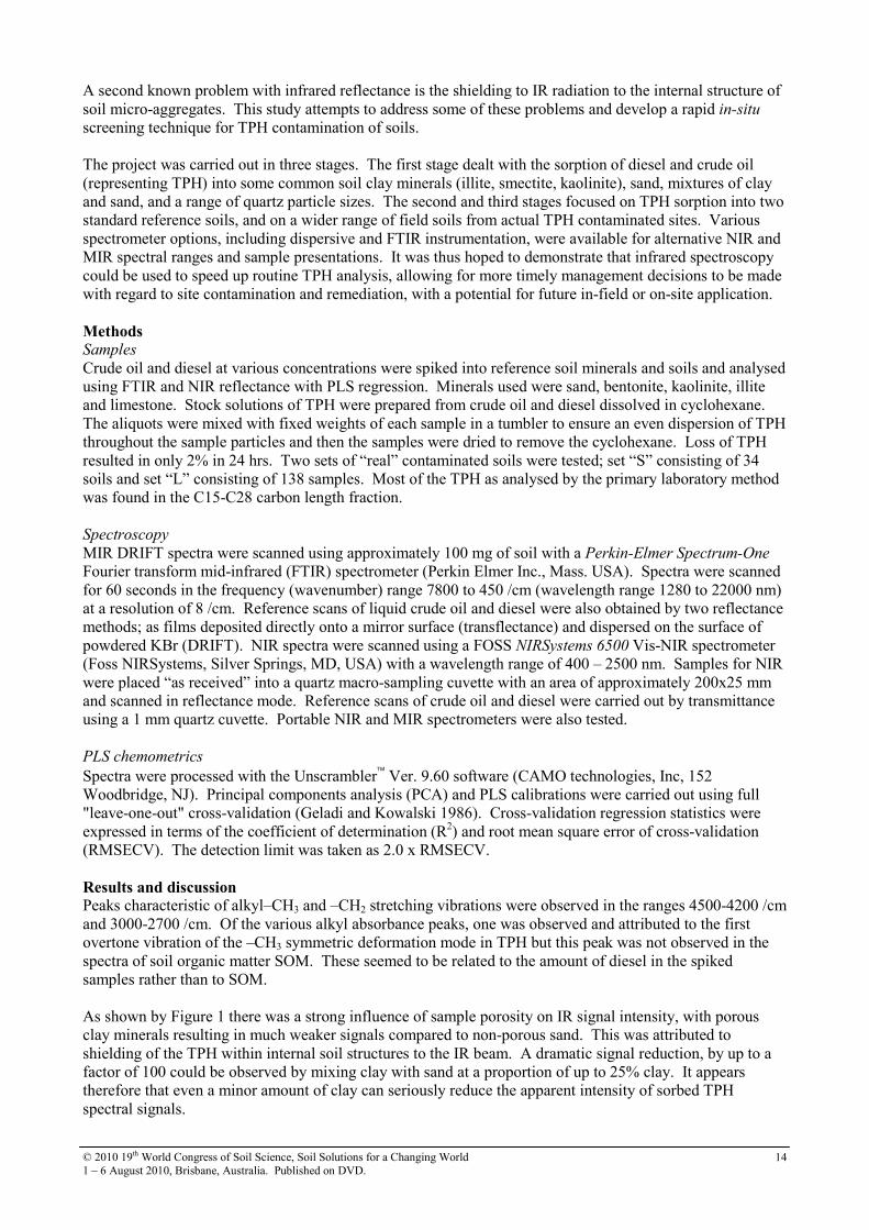
As shown by Figure 1 there was a strong influence of sample porosity on IR signal intensity, with porous
clay minerals resulting in much weaker signals compared to non-porous sand. This was attributed to
shielding of the TPH within internal soil structures to the IR beam. A dramatic signal reduction, by up to a
factor of 100 could be observed by mixing clay with sand at a proportion of up to 25% clay. It appears
therefore that even a minor amount of clay can seriously reduce the apparent intensity of sorbed TPH
spectral signals.
© 2010 19th World Congress of Soil Science, Soil Solutions for a Changing World
1 – 6 August 2010, Brisbane, Australia. Published on DVD. 15
Crude - differences
-0.1
0.0
0.1
0.2
0.3
0.4
0.5
0.6
0.7
2500 3500 4500
diff-Cka
diff-Cil
diff-CS
diff-CSm
diff-CCO3
Figure 1 DRIFT spectra of crude oil adsorbed onto soil minerals from a 1% solution of crude in cyclohexane.
(diff-Cka) kaolinite, (diff-Cil) illite, (diff-CS) sand, (diff-Sm) smectite, (diff-CCO3) carbonate. Crude oil spectra
were derived by difference between spiked mineral spectra and raw minerals.
PLS cross-validation results for crude oil spiked into soil minerals are shown in Table 1. Prediction errors
(RMSECV) ranged from 700 to 4,200 mg/kg, depending on the range of crude oil in the PLS models. Errors
were higher for the NIR portion of the FTIR spectra, although the NIRS6500 gave better results for sand and
smectite.
Table 1. PLS cross-validation prediction of TPH in reference minerals. Standard errors (RMSECV) are shown
in parentheses.
Mineral Crude oil FTIR (MIR) FTIR (NIR) NIRS6500
(mg/kg) (RMSECV mg/kg) (RMSECV mg/kg) (RMSECV mg/kg)
Kaolinite 0-10,000 700
Illite 0-10,000 1900
Smectite 0-100,000 2400 6300 2600
Carbonate 0-100,000 4200 4500
Quartz 0-100,000 3900 8000 3000
Results for the reference standard soils were also considered to be reasonable, with RMSECV values ranging
from approximately 2,500 ppm in the 0-25,000 ppm range (REF1) to 1,700 ppm in the 0-10,000 ppm range.
Similar results were obtained for the FT-NIR. Cross-validation errors were therefore approximately 10% of
the range of TPH in the calibration sets.
During the course of studies a number of very weak spectral peaks, apparently unique to TPH, were detected
in the MIR –CH stretching frequency range. These peaks were attributed to combination and overtone
vibrational frequencies of terminal methyl (-CH3) chemical groups found in higher proportion in diesel and
crude oil than in the longer chain length soil organic matter, and thus important for the accurate
determination of TPH in a wide range of soils in the presence of SOM. Prediction accuracy appeared to be
enhanced when these signatures were used, since they could be used to separate the IR signals for short-chain
terminal –CH3 groups in diesel and crude oil from those of long-chain hydrocarbons in the native SOM.
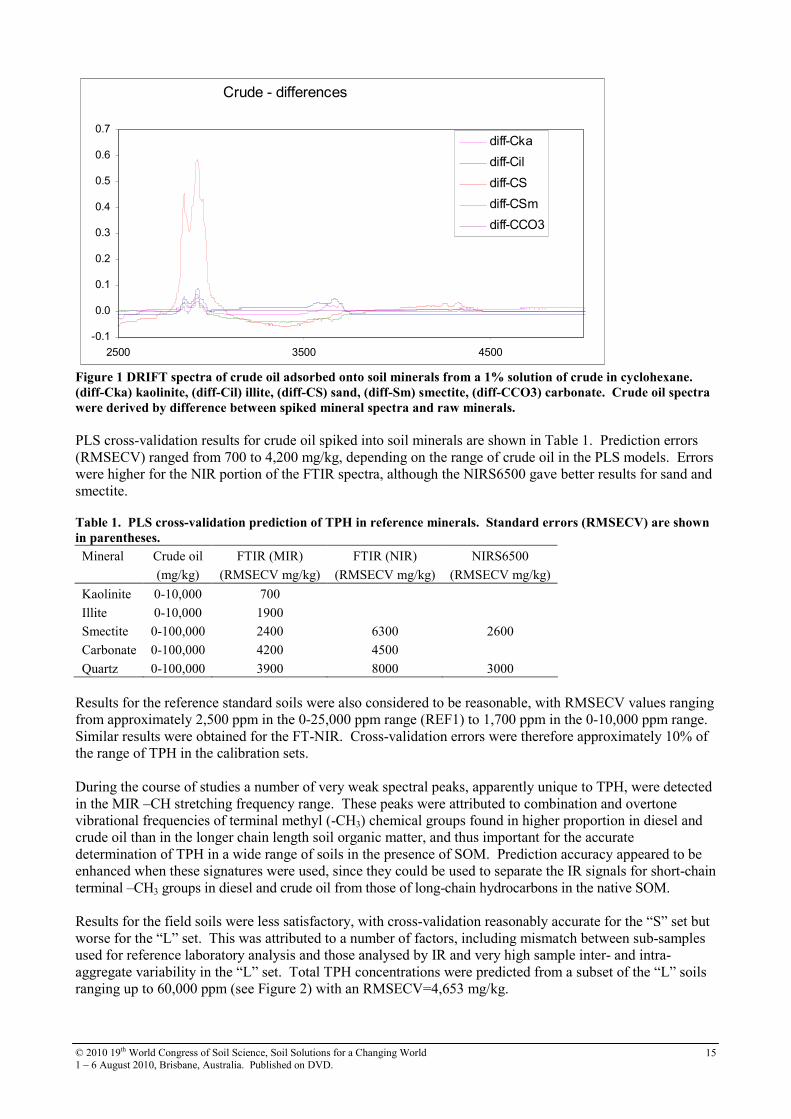
Results for the field soils were less satisfactory, with cross-validation reasonably accurate for the “S” set but
worse for the “L” set. This was attributed to a number of factors, including mismatch between sub-samples
used for reference laboratory analysis and those analysed by IR and very high sample inter- and intra-
aggregate variability in the “L” set. Total TPH concentrations were predicted from a subset of the “L” soils
ranging up to 60,000 ppm (see Figure 2) with an RMSECV=4,653 mg/kg.
© 2010 19th World Congress of Soil Science, Soil Solutions for a Changing World
1 – 6 August 2010, Brisbane, Australia. Published on DVD. 16
Figure 2. FT-MIR PLS calibration for total TPH derived from 35 “L” samples.
Conclusions It was concluded from this preliminary study that the MIR DRIFT method could satisfy the required
accuracy requirements for field screening, provided that certain experimental conditions could be met; the
same sub-sample must be used for each training/validation IR and laboratory measurement as far as possible,
the peaks used to build the IR calibration models use the most effective spectral signatures, and minimal
TPH is lost between receipt of samples and sample scanning, the predicted TPH values for field screening
are offset or normalised by a few reference laboratory control data, and surface area, particle size and surface
effects are taken into account. An encouraging finding of this study was the possibility of being able to
discriminate between TPH and SOM which current techniques are unable to do. This study suggests that,
with recent availability of truly field portable MIR spectrometers, the in-situ measurement of contaminants in
soils has become more feasible.
Acknowledgements The Authors would like to thank the CSIRO land and Water executive for allocating funds from the CSIRO
“innovation bank” for the initial stages of this work, and Ziltek Pty Ltd for additional funding, provision of
samples and data for this project work.
References Malley DF, Hunter KN, Webster GRB (1999) Analysis of diesel fuel contamination in soils by near-infrared
reflectance spectrometry and solid phase microextraction-gas chromatography. Journal of Soil
Contamination 8, 481-489.
Geladi P, Kowalski BR (1986) Partial least-squares regression: a tutorial. Analytica Chimica Acta 185, 1–17.
y = 0.7891x + 2362.2
R2 = 0.8137
0
10000
20000
30000
40000
50000
60000
0 10000 20000 30000 40000 50000 60000 70000
TPH (mg.Kg-1)
TPH (DRIFT m
g.Kg-1)
TPH (mg/kg)
TPH (DRIFT m
g/kg)
© 2010 19th World Congress of Soil Science, Soil Solutions for a Changing World
1 – 6 August 2010, Brisbane, Australia. Published on DVD. 17
Application of LS-SVM-NIR spectroscopy for carbon and nitrogen prediction in
soils under sugarcane
Sandra Oliveira SáA,, Marco Flores Ferrão
B, Marcelo Valadares Galdos
C, Carla Maris Machado Bittar
D and
Ronei Jesus PoppiE
AUniversidade Estadual do Maranhão, São Luis, MA, 65055-310. Brazil, E-mail: [email protected] BUniversidade de Santa Cruz do Sul, 96815-900, Santa Cruz do Sul, RS, Brazil. CCentro de Energia Nuclear na Agricultura, Universidade de São Paulo, 13400-970, Piracicaba, SP, Brazil. DEscola Superior de Agricultura “Luiz de Queiroz”, Universidade de São Paulo, 13418-900, Piracicaba, SP, Brazil. EInstituto de Química, Universidade Estadual de Campinas, 13083-970, Campinas, SP, Brazil.
Abstract In this paper, Least-Square Support Vector Machine (LS-SVM) regression is used to for a rapid and accurate
quantification of total carbon (total-C) and total nitrogen (total-N) in soil samples collected in forest and
sugarcane areas in Sao Paulo State, Brazil. NIRS spectra were recorded on a NIRS 5000 scanning
monochromator. The concentration ranges of 0.401-3.101 %, for total-C, and 0.030-0.252 %, for total-N
were obtained for the references. The performance and robustness of LS-SVM regression are compared to
Partial Least Square Regression (PLSR). For total-C, correlation coefficients (R2cal) of 0.99 and 0.92,
RMSECV of 0.132 and 0.176 %, and RMSEP of 0.110 and 0.141 % were obtained for LS-SVM and PLSR,
respectively. For total-N, correlation coefficients (R2cal) of 0.98 and 0.92, RMSECV of 0.015 and 0.013 %,
and RMSEP of 0.008 and 0.009 % were obtained for LS-SVM and PLSR, respectively. At the same time,
results indicate that LS-SVM-NIRS can be used with advantage as an analytical method for rapid, accurate,
reliable and cost-effective routine analysis of total carbon and nitrogen in tropical soil.
Key Words NIR, chemometrics, sugarcane, tropical soil, carbon, nitrogen.
Introduction The Support Vector Machine (SVM) is a relatively new nonlinear technique in the field of chemometrics and
is employed basically in classification and multivariate calibration problems (Thissen et al. 2003). Recently
an extension of SVM, called Least Square Support Vector Machines (LS-SVM) was introduced (Codgill and
Dardenne, 2004). LS-SVM is capable of dealing with linear and nonlinear multivariate calibration and
resolves multivariate calibration problems in a relatively fast way. In the LS-SVM a linear function (y = w x
+ b) is fitted between the dependent (y) and independent (x) variables. As in SVM, it is necessary to
minimize a cost function (L) containing a penalized regression error. The aim of this work was to propose
the use of least-squares support vector machine (LS-SVM) and NIR spectroscopy with diffuse reflectance as
a methodology for quantification of total carbon (total-C) and total nitrogen (total-N) in Brazilian soils from
sugarcane cultivation. Brazil is today the largest sugarcane produce in the world attaining nearly 5 million
hectares of planted area to produce 643,7 million tones of cane stalks in the 2007/08 season. About 386
million tones are produced in the State of Sao Paulo alone.
Methods Study area and sampling
A total of 250 soil samples (0-100 cm depth) were collected in a sugarcane plantation located in Pradópolis
(210 22’ of S. 48
0 03’ W.) in São Paulo State, Brazil. The soil is a Typic Haplodux, with clayey texture.
According to the Köppen classification, the climate is an Aw type, tropical wet with a dry winter, with
average annual precipitation close to 1,560 mm/year. The average annual air temperature is 22.9 oC, and the
average monthly temperatures are above 18.0 oC. Sugarcane had been grown for the factory for at least fifty
years. Four fields with mechanical pre-harvesting were selected, using the method of chronossequence,
where sugarcane had been harvested, without replanting or soil disturbance, for 8, 6, 4, and 2 years. Soil
samples were also collected in an area of native forest, as a reference. The sampling was done in a grid
system with nine replications in each field, to depths of 0-10, 10-20, 20-30, 40-50, 70-80 and 90-100 cm.
Reference analyses and Spectral measurements
Samples were air-dried, sieved and grounded to 60 mesh before analysis. Reference analyses for total C and
total N were performed by dry combustion on a LECO CN 2000 elemental analyzer (furnace at 1200 0C in
© 2010 19th World Congress of Soil Science, Soil Solutions for a Changing World
1 – 6 August 2010, Brisbane, Australia. Published on DVD. 18
pure oxygen). The principle is to convert all the different forms of carbon into CO2 to be measured
quantitatively by infrared. In addition, the combustion process converts any nitrogen forms into N2 and NOx
and an aliquot of the sample gas is purified by catalyst heater (NOx gas are reduced to N2), Lecosorb (to
remove CO2) and Anhydrone (to remove H2O). Then the N2 can be measured by thermoelectric detector.
NIRS spectra were recorded on a NIRS 5000 scanning monochromator (Foss NIRSystems, MD). Sample
ware scanned in a spinning micro sample cup and the spectra were recorded at 2-nm intervals in the range of
1100 - 2498 nm by using WINISI II version 1.05 software (Infrasoft International, Silver Spring, MD) for
data acquisition. A ceramic standard was used for the background spectra and the spectra was collected as
log(1/R), where R is reflectance. For NIR calibration, two multivariate regression methods were used: (i)
NIR-PLS using the PLS program from PLS-Toolbox version 3.5 with Matlab from Eigenvector Research
Inc. (Wise et al. 2005); and (ii) NIR-LS-SVM using the LS-SVMlab (Matlab/C Toolbox for Least Squares
Support Vector Machines) (Suykens et al. 2002). All programs were run on an IBM-compatible Intel
Pentium 4 CPU 3.00 GHz and 1 Gbyte RAM microcomputer. Data were treated using a multiplicative
scattered correction (MSC) technique before further multivariate analysis. To evaluate the error of each
calibration model, the root mean square error was used, calculated by eq. 1.
(1)
Results All spectra were pre-processed by multiplicative scatter correction (MSC), aiming at correcting the baseline
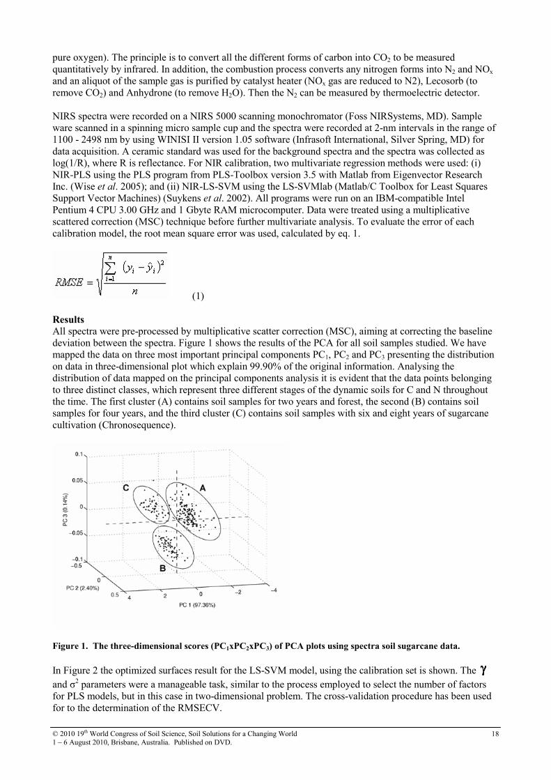
deviation between the spectra. Figure 1 shows the results of the PCA for all soil samples studied. We have
mapped the data on three most important principal components PC1, PC2 and PC3 presenting the distribution
on data in three-dimensional plot which explain 99.90% of the original information. Analysing the
distribution of data mapped on the principal components analysis it is evident that the data points belonging
to three distinct classes, which represent three different stages of the dynamic soils for C and N throughout
the time. The first cluster (A) contains soil samples for two years and forest, the second (B) contains soil
samples for four years, and the third cluster (C) contains soil samples with six and eight years of sugarcane
cultivation (Chronosequence).
Figure 1. The three-dimensional scores (PC1xPC2xPC3) of PCA plots using spectra soil sugarcane data.
In Figure 2 the optimized surfaces result for the LS-SVM model, using the calibration set is shown. The γγγγ
and σ2 parameters were a manageable task, similar to the process employed to select the number of factors
for PLS models, but in this case in two-dimensional problem. The cross-validation procedure has been used
for to the determination of the RMSECV.
© 2010 19th World Congress of Soil Science, Soil Solutions for a Changing World
1 – 6 August 2010, Brisbane, Australia. Published on DVD. 19
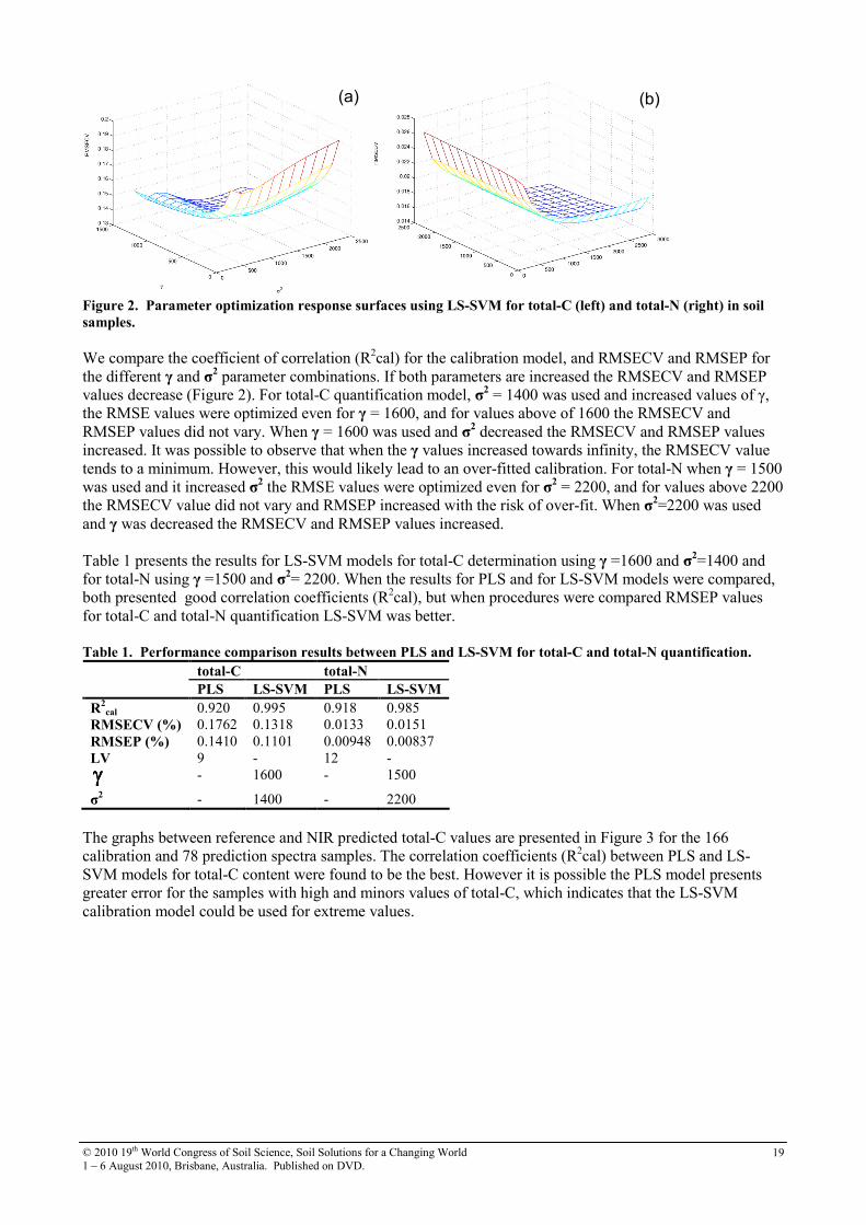
(a) (b)(a) (b)
Figure 2. Parameter optimization response surfaces using LS-SVM for total-C (left) and total-N (right) in soil
samples.
We compare the coefficient of correlation (R2cal) for the calibration model, and RMSECV and RMSEP for
the different γ and σ2 parameter combinations. If both parameters are increased the RMSECV and RMSEP
values decrease (Figure 2). For total-C quantification model, σ2 = 1400 was used and increased values of γ,
the RMSE values were optimized even for γ = 1600, and for values above of 1600 the RMSECV and
RMSEP values did not vary. When γ = 1600 was used and σ2 decreased the RMSECV and RMSEP values
increased. It was possible to observe that when the γ values increased towards infinity, the RMSECV value
tends to a minimum. However, this would likely lead to an over-fitted calibration. For total-N when γ = 1500
was used and it increased σ2 the RMSE values were optimized even for σ
2 = 2200, and for values above 2200
the RMSECV value did not vary and RMSEP increased with the risk of over-fit. When σ2=2200 was used
and γ was decreased the RMSECV and RMSEP values increased.
Table 1 presents the results for LS-SVM models for total-C determination using γ =1600 and σ2=1400 and
for total-N using γ =1500 and σ2= 2200. When the results for PLS and for LS-SVM models were compared,
both presented good correlation coefficients (R2cal), but when procedures were compared RMSEP values
for total-C and total-N quantification LS-SVM was better.
Table 1. Performance comparison results between PLS and LS-SVM for total-C and total-N quantification.
total-C total-N
PLS LS-SVM PLS LS-SVM
R2cal 0.920 0.995 0.918 0.985
RMSECV (%) 0.1762 0.1318 0.0133 0.0151
RMSEP (%) 0.1410 0.1101 0.00948 0.00837
LV 9 - 12 -
γγγγ - 1600 - 1500
σ2 - 1400 - 2200
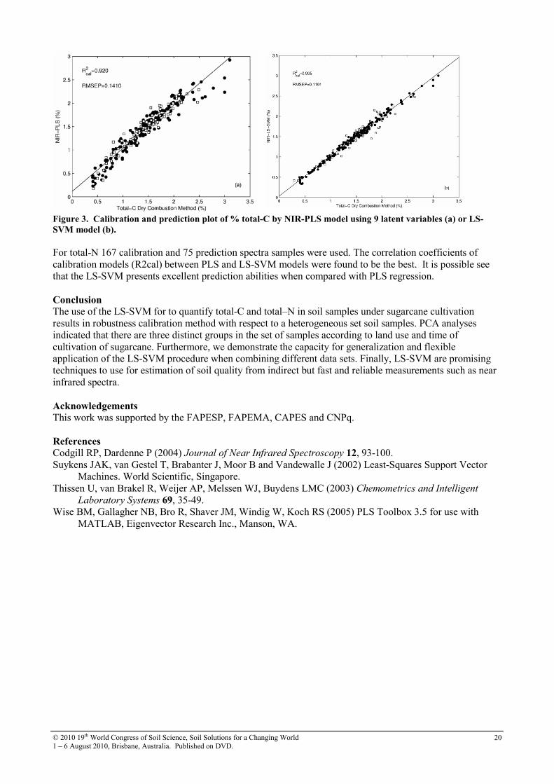
The graphs between reference and NIR predicted total-C values are presented in Figure 3 for the 166
calibration and 78 prediction spectra samples. The correlation coefficients (R2cal) between PLS and LS-
SVM models for total-C content were found to be the best. However it is possible the PLS model presents
greater error for the samples with high and minors values of total-C, which indicates that the LS-SVM
calibration model could be used for extreme values.
© 2010 19th World Congress of Soil Science, Soil Solutions for a Changing World
1 – 6 August 2010, Brisbane, Australia. Published on DVD. 20
Figure 3. Calibration and prediction plot of % total-C by NIR-PLS model using 9 latent variables (a) or LS-
SVM model (b).
For total-N 167 calibration and 75 prediction spectra samples were used. The correlation coefficients of
calibration models (R2cal) between PLS and LS-SVM models were found to be the best. It is possible see
that the LS-SVM presents excellent prediction abilities when compared with PLS regression.
Conclusion The use of the LS-SVM for to quantify total-C and total–N in soil samples under sugarcane cultivation
results in robustness calibration method with respect to a heterogeneous set soil samples. PCA analyses
indicated that there are three distinct groups in the set of samples according to land use and time of
cultivation of sugarcane. Furthermore, we demonstrate the capacity for generalization and flexible
application of the LS-SVM procedure when combining different data sets. Finally, LS-SVM are promising
techniques to use for estimation of soil quality from indirect but fast and reliable measurements such as near
infrared spectra.
Acknowledgements This work was supported by the FAPESP, FAPEMA, CAPES and CNPq.
References Codgill RP, Dardenne P (2004) Journal of Near Infrared Spectroscopy 12, 93-100.
Suykens JAK, van Gestel T, Brabanter J, Moor B and Vandewalle J (2002) Least-Squares Support Vector
Machines. World Scientific, Singapore.
Thissen U, van Brakel R, Weijer AP, Melssen WJ, Buydens LMC (2003) Chemometrics and Intelligent
Laboratory Systems 69, 35-49.
Wise BM, Gallagher NB, Bro R, Shaver JM, Windig W, Koch RS (2005) PLS Toolbox 3.5 for use with
MATLAB, Eigenvector Research Inc., Manson, WA.
© 2010 19th World Congress of Soil Science, Soil Solutions for a Changing World
1 – 6 August 2010, Brisbane, Australia. Published on DVD. 21
Acquisition and reliability of geophysical data in soil science
Anne-Kathrin Nüsch A, Peter Dietrich
A, Ulrike Werban
A, Thorsten Behrens
B
A Department of Monitoring and Exploration Technologies, Helmholtz Centre for Environmental Research – UFZ, Permoser Straße
15, 04318 Leipzig, Germany, [email protected] B
Faculty of Geoscience, University of Tübingen, Rümelinstraße 19-23, 72070 Tübingen, Germany
Abstract We present results of the EU- funded project iSOIL (Interactions between soil related sciences- Linking
geophysics, soil science and digital soil mapping). One focus of iSOIL is the acquisition and combination of
different geophysical data for proximal soil sensing and the evaluation of single geophysical methods
according to their reliability. The data acquisition follows a concept, which combines different scales from
plot scale to point sampling. This strategy is enabled by the application of mobile geophysical platforms,
which allow fast and flexible measurements. Furthermore it is possible to mount different instruments on
platforms and combine them.
A prerequisite for the common interpretation of different methods is the reproducibility of data of a single
method. We present results concerning reproducibility of Electromagnetic induction (EMI) – data. EMI data
depend on many factors which are also caused by the instrument itself. We investigated following aspects:
1) Comparison of two identical EM38DD-instruments
2) Comparison of the calibration of different persons
3) Variation of calibration height
In our presentation we show which facts have to be regarded during calibration procedure.
Key words Measuring design, hierarchical approach, combination of methods, electromagnetic induction, reliability of
data.
Introduction The focus of the project iSOIL “Interactions between soil related sciences – Linking geophysics, soil science
and digital soil mapping” is to develop new and to improve existing strategies and innovative methods for
generating accurate, high-resolution soil property maps. At the same time the developments will reduce costs
compared to traditional soil mapping. The project tackles this challenge by integrating the following three
major components:
• high resolution, non-destructive geophysical (e.g. electromagnetic induction - EMI; ground
penetrating radar, magnetics, seismics) and spectroscopic methods,
• spatial inter- and extrapolations (e.g. geostatistics, machine learning) concepts (McBratney et al.
2003), and
• soil sampling and validation schemes to provide representative and transferable results (Brus, et al.
2006; de Gruiter, et al. 2009; Behrens et al. 2006).
Thus, within iSOIL we will develop, validate, and evaluate concepts and strategies for transferring measured
physical parameter distributions into soil property, soil function and soil threat maps of different scales,
which are relevant to and demanded by the “Thematic Strategy for Soil Protection” (European Commission
2006). The final aim of the iSOIL project is to provide techniques and recommendations for high resolution,
economically feasible, and target- oriented soil mapping under conditions which are realistic for end-user.
The resulting soil property maps can be used for precision agriculture applications and soil degradation
threats studies, e.g. erosion, compaction and soil organic matter decline.
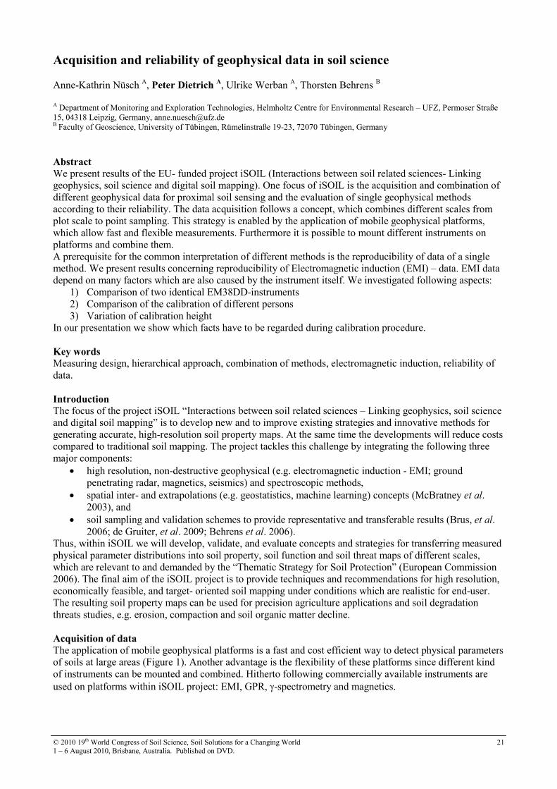
Acquisition of data The application of mobile geophysical platforms is a fast and cost efficient way to detect physical parameters
of soils at large areas (Figure 1). Another advantage is the flexibility of these platforms since different kind
of instruments can be mounted and combined. Hitherto following commercially available instruments are
used on platforms within iSOIL project: EMI, GPR, γ-spectrometry and magnetics.
© 2010 19th World Congress of Soil Science, Soil Solutions for a Changing World
1 – 6 August 2010, Brisbane, Australia. Published on DVD. 22
Figure 1. Mobile geophysical platform: EM31 (1
st sledge) and EM38DD (2
nd sledge) are towed by a tractor.
Since geophysical methods provide only physical parameters it is essential to combine them with
conventional soil sampling methods for ground truthing. Via transfer functions physical parameters have to
be converted into soil parameters. We need to develop measuring designs for the evaluation and combination
of different geophysical methods. The application of a hierarchical approach is one way to combine different
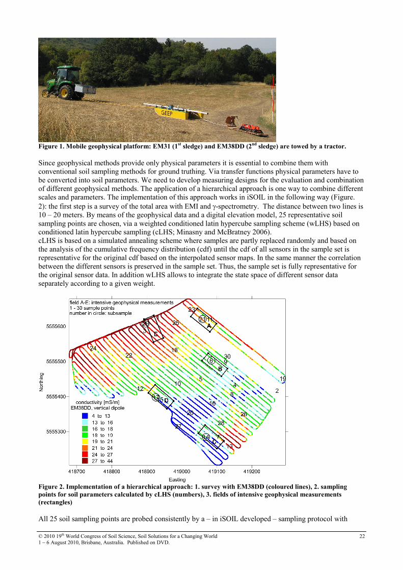
scales and parameters. The implementation of this approach works in iSOIL in the following way (Figure.
2): the first step is a survey of the total area with EMI and γ-spectrometry. The distance between two lines is
10 – 20 meters. By means of the geophysical data and a digital elevation model, 25 representative soil
sampling points are chosen, via a weighted conditioned latin hypercube sampling scheme (wLHS) based on
conditioned latin hypercube sampling (cLHS; Minasny and McBratney 2006).
cLHS is based on a simulated annealing scheme where samples are partly replaced randomly and based on
the analysis of the cumulative frequency distribution (cdf) until the cdf of all sensors in the sample set is
representative for the original cdf based on the interpolated sensor maps. In the same manner the correlation
between the different sensors is preserved in the sample set. Thus, the sample set is fully representative for
the original sensor data. In addition wLHS allows to integrate the state space of different sensor data
separately according to a given weight.
Figure 2. Implementation of a hierarchical approach: 1. survey with EM38DD (coloured lines), 2. sampling
points for soil parameters calculated by cLHS (numbers), 3. fields of intensive geophysical measurements
(rectangles)
All 25 soil sampling points are probed consistently by a – in iSOIL developed – sampling protocol with
© 2010 19th World Congress of Soil Science, Soil Solutions for a Changing World
1 – 6 August 2010, Brisbane, Australia. Published on DVD. 23
conventional soil sampling methods with regard to texture, organic matter content, etc. Out of these sampling
points five points are chosen for further detailed measurements. Around a single point a small area of 30 x 70
meters is placed to accomplish geophysical high resolution measurements. Besides EMI and γ-spectrometry
also magnetics, seismics and GPR are applied. The line distance is only one meter and also the towing-
velocity is slow.
The combination and common interpretation of different methods require several prerequisites to a single
method. The measurements need to be comparable within several fields and over time. As a representative
we show in the following results of a comparability study with the EMI instrument EM38DD.
Reproducibility of electromagnetic induction measurements in the near surface area EM38DD is a widely-spread instrument for near surface applications to detect electrical conductivity of the
subsurface. Among others it is used in the field of precision agriculture. The measured signal depends on
many internal (caused by the instrument) and external criteria, hence measured data can be used only for
qualitative interpretation.
In particular for monitoring aspects the data need to be reproducible in a quantitative manner additionally.
External criteria are weather conditions as well as water content of soils and cannot be influenced. The
second group of criteria implies calibration of the instrument and changes in electronics of the instrument
over time.
A field campaign focused on internal factors and the results show serious differences in single
measurements. At all we measured 30 test series on two lines regarding following factors:
1) Comparison of two identical EM38DD-instruments
2) Comparison of the calibration of different persons
3) Variation of calibration height
The influence of the factors needs to be regarded for horizontal and vertical dipole separately.
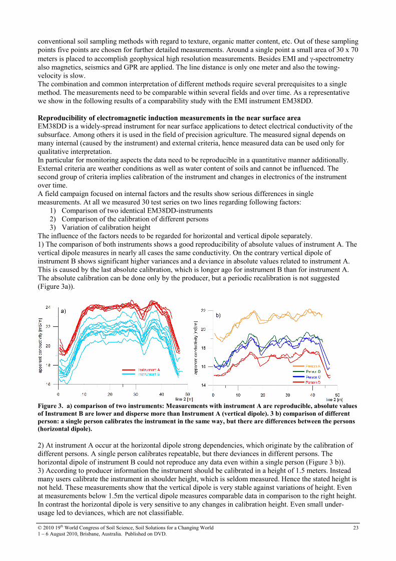
1) The comparison of both instruments shows a good reproducibility of absolute values of instrument A. The
vertical dipole measures in nearly all cases the same conductivity. On the contrary vertical dipole of
instrument B shows significant higher variances and a deviance in absolute values related to instrument A.
This is caused by the last absolute calibration, which is longer ago for instrument B than for instrument A.
The absolute calibration can be done only by the producer, but a periodic recalibration is not suggested
(Figure 3a)).
Figure 3. a) comparison of two instruments: Measurements with instrument A are reproducible, absolute values
of Instrument B are lower and disperse more than Instrument A (vertical dipole). 3 b) comparison of different
person: a single person calibrates the instrument in the same way, but there are differences between the persons
(horizontal dipole).
2) At instrument A occur at the horizontal dipole strong dependencies, which originate by the calibration of
different persons. A single person calibrates repeatable, but there deviances in different persons. The
horizontal dipole of instrument B could not reproduce any data even within a single person (Figure 3 b)).
3) According to producer information the instrument should be calibrated in a height of 1.5 meters. Instead
many users calibrate the instrument in shoulder height, which is seldom measured. Hence the stated height is
not held. These measurements show that the vertical dipole is very stable against variations of height. Even
at measurements below 1.5m the vertical dipole measures comparable data in comparison to the right height.
In contrast the horizontal dipole is very sensitive to any changes in calibration height. Even small under-
usage led to deviances, which are not classifiable.

© 2010 19th World Congress of Soil Science, Soil Solutions for a Changing World
1 – 6 August 2010, Brisbane, Australia. Published on DVD. 24
If these factors accumulate, it is nearly impossible to measure reproducible data. For that reason we need to
develop methods, how to evaluate the single factors and how to unify the calibration procedure.
Conclusion Within EU-funded project iSOIL we combine different mobile geophysical method for fast and efficient soil
mapping. The major prerequisite for combining is the reliability and reproducibility of data of each single
methode. As an example we show results of electromagnetic induction measurements. The focus of this
poster is to compare three different man made factors that influence electromagnetic induction
measurements: the instruments itself, the influence of the person who calibrates and the calibration height.
The results show strong deviances between different instruments of the same type (EM38DD). Furthermore
the measured values depend on the person who is calibrating the instrument. And at least the variation of
height of calibration leads to non-classifiable variations in measured values.
Due to these factors it is necessary difficult to measure quantitative values for monitoring aspects, but errors
can be minimized by reducing changes in calibration height, using always the same instrument and only one
person should calibrate within one field campaign.
In addition to this contribution please see the poster presentation „iSOIL and Standardization“ for details on
one activity of the iSOIL project: the CEN Workshop to establish a widely accepted voluntary standard for a
best practice of EMI- measurements.
References Behrens T, Scholten T (2006) Digital soil mapping in Germany - a review. J. Plant Nutr.Soil Sci. 169, 434-
443.
Brus DJ, de Gruijter JJ, van Groenigen JW (2006) Designing spatial coverage samples using the k-means
clustering algorithm. In: ‘Digital Soil Mapping: An Introductory Perspective. Developments in Soil
Science’. (Eds. P Lagacherie, A McBratney, M Voltz), Vol. 3, (Elsevier Publishing: Amsterdam)
de Gruijter JJ, McBratney AB, Taylor J (2009) Sampling for High Resolution Soil Mapping.
European Commission (2006) Thematic Strategy for Soil Protection Communication. COM (2006) 231.
McBratney AB, Santos MLM, Minasny B (2003) On digital soil mapping. Geoderma 117, 3-52
Minasny B, McBratney AB (2006) A conditioned Latin hypercube method for sampling in the presence of
ancillary information. Computers & Geosciences 32, 1378–1388.
© 2010 19th World Congress of Soil Science, Soil Solutions for a Changing World
1 – 6 August 2010, Brisbane, Australia. Published on DVD. 25
Assessment of soil variation by multivariate geostatistical analysis of EMI and
gamma-radiometric data Annamaria Castrignanò
A, Mike T F Wong
B and Francesca Guastaferro
A
ACRA-SCA via Celso Ulpiani, 5. Bari-Italy, Email [email protected] BCSIRO Land and Water, Wembley, Western Australia WA 6014, Email [email protected]
Abstract An EMI survey provides data on the apparent soil electrical conductivity of the soil profile and this is often
locally correlated with soil properties such as texture and pH. Occurrence of salinity, gravels and rocks in the
landscape interferes with interpretation of the data. Complementary measurements are often used to infer soil
properties. We surveyed a 200 ha cropping field in Western Australia with EMI and complementary gamma-
ray spectrometer to delineate management zones. We applied a multivariate approach called multi collocated
factor cokriging using seven variables measured during the survey: natural gamma-emission from potassium,
thorium, uranium, total emission, measurements from two EMI sensors (EM38, EM31) and GPS height. A
salty stream along the north-west boundary of the field influenced the spatial pattern of variation. The first
anisotropic factor along the direction of the stream had a range of 900m and was mostly influenced by k
emission. On the contrary, the first factor at shorter range on the orthogonal direction to the flow of the creek
was dominated by topography. Factor cokriging resulted in partitioning of the field into three areas using the
interquantile values as breakdown points after filtering outliers. The resulting spatial classification did not
show clear spatial long-range structures.
Key Words Management zones, electromagnetic induction, gamma emission, geostatistics, factor cokriging, GPS.
Introduction Variation in soil properties across a field interacts with seasonal conditions and management to give rise to
large variations in crop yields, deep drainage and nitrate leaching in rain-fed Mediterranean-type
environment (Wong et al. 2006; Wong and Asseng 2006). This results in corresponding variation in fertiliser
requirement. Delineation of management zones to represent clustering of soil properties relevant to crop
productivity allows increased precision in field management. Traditional clustering techniques produce
natural groupings of soil data in the attribute space without reference to geographical position, which may
cause several spots of disjoint clusters to occur. We then preferred to use a multivariate geostatistical
approach, based on Principal Component Analysis and called multi collocated factor cokriging, to enable us
to estimate some synthetic indices describing the continuous spatial variation in the soils (Castrignanò et al.
2000).
An EMI survey provides data on the apparent soil electrical conductivity of the soil profile and this is often
locally correlated with soil properties such as texture, plant available soil water storage capacity and pH.
EMI-based methods cannot distinguish between sandy soils and gravels which have similar and low apparent
electrical conductivities (ECa). To overcome these shortcomings, we complemented EMI with gamma-
radiometric survey which shows promise in high resolution soil property mapping (Wong et al. 2009). The
spectrometer measures natural γ-emissions from the top 30-45 cm of the soil due to emitters such as 40
K and
daughter radionuclides of 238
U and 232
Th. Ambiguity in the interpretation of radiometric data arises when
soils with varying gravel and clay contents occur across the surveyed area: increases in clay content or
proximity of gravels to the soil surface both result in strong signals. This problem is not encountered with
ECa-based methods since clays and gravels give rise to markedly different ECa-values.
The objective of this work was to apply a multivariate geostatistical approach for delineating management
zones based on complementary EMI and gamma-radiometric survey to improve management of field
variation.
Methods The 200 ha cropping field is situated 350 km north of Perth, at Buntine in Western Australia. We
simultaneously measured (1) apparent soil electrical conductivity (ECa) across the field on 30 m line spacing
with electromagnetic induction equipments (EM31, EM38 GEONICS, Ltd, Ontario-Canada), (2) γ-ray

© 2010 19th World Congress of Soil Science, Soil Solutions for a Changing World
1 – 6 August 2010, Brisbane, Australia. Published on DVD. 26
emission using an Exploranium γ-ray spectrometer with a large (8 l) thallium activated sodium iodide crystal
scintillation detector and (3) differential corrected GPS location. ECa, γ-ray emission and GPS location were
recorded at 1 second intervals. The γ-ray spectra were resolved into the individual emissions from potassium,
thorium and uranium according to their characteristic peaks.
Geostatistical analysis
Even if ordinary cokriging does not require the data to follow a normal distribution, variogram modelling is
sensitive to strong departures from normality. Therefore, we transformed each initial attribute into a
Gaussian-shaped variable with zero mean and unit variance (Chilès and Delfiner 1999)
To produce the maps of the original variables and of synthetic scale-dependent indices of spatial dependence,
the multivariate spatial data were analysed by multi collocated cokriging and Factor Cokriging Analysis
(FCKA) (Wackernagel 2003). The latter consists of a scale-dependent decomposition of the set of original
second-order random stationary variables into a set of reciprocally orthogonal regionalized factors. The
approach efficiently uses the auxiliary variable only at the target grid node and at all the locations where the
primary variable is defined (Rivoirard 2001).
Results Distributions of ECa, gamma-radiometric values were found to be strongly positively skewed (skewness
varying between 1.37 and 2.31), whereas height distribution was symmetric (skewness = 0.02) but bimodal.
An anisotropic LMC was fitted because the field slopes towards a salty creek, which forms its north-west
boundary, and this creek drives zonal anisotropy along the direction 60 N, characterised by greater continuity
(longer range and smaller sill) compared with the other directions. The model includes four basic structures:
1) a nugget effect, 2) an isotropic cubic model with range= 400 m, 3) an anisotropic Bessel K model in
direction N150 with range = 500 m and parameter=1 and 4) an anisotropic Bessel K model in direction N60
with range = 900 m and parameter=1. The estimated maps are reported in fig.1 and show more uncertainty
along the western boundary due to the scarcity of samples in the interpolation neighbourhood. Thorium,
uranium and total counts look quite similar, whereas the information obtained from the potassium channel
differs (Wong et al. 2009).
Low EM38 values of <10 mS/m, occurring approximately along the axis 442000 east, coincides
approximately with a similar area for low emission from K. Areas of high EM38 values >45 mS/m,
occurring along the western boundary of the field due to the presence of a salty creek, are not matched by
high gamma-radiometric values.
To synthesise the multivariate variation of the field, the multi collocated factor cokriging analysis was
applied to the seven Gaussian transformed variables. The sum of the eigenvalues at each spatial scale gives
an estimation of variance at that scale. The main components of variation (about 44 and 36% of the total
variance) occur at longer range (900 m) along the creek direction and in the orthogonal direction at shorter
range (500 m), respectively. On the contrary, the contributions of the isotropic and the spatially uncorrelated
(nugget effect) component to the total variance are lower (16% and 4%, respectively).
Only the eigenvectors producing eigenvalues greater than one should be retained, because their variation is
assumed statistically different from residual variation. We focused in particular on the first factor at shorter
and longer scale, which account for about 59% and 72% of the variation at the corresponding spatial scales,
respectively. The loading values for the two factors indicate elevation and the radionuclides as the most
inversely influencing the first factor at shorter range along the direction N150, whereas K and total gamma–
ray emissions, and elevation and EM38 data at a less extension, weigh positively on the long range factor
along the direction of the creek. All the variables, with the exception of elevation and k emissions, affect the
isotropic variation at short range, but EMI data do that positively whereas gamma emissions negatively.
Summarising we could say that there are three main factors controlling the spatial variation of this field:
salinity, acting along the direction of the creek flow, topography along the orthogonal direction to the flow
and texture acting isotropically.
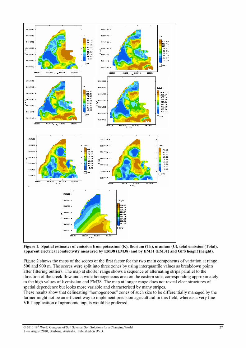
© 2010 19th World Congress of Soil Science, Soil Solutions for a Changing World
1 – 6 August 2010, Brisbane, Australia. Published on DVD. 27
Figure 1. Spatial estimates of emission from potassium (K), thorium (Th), uranium (U), total emission (Total),
apparent electrical conductivity measured by EM38 (EM38) and by EM31 (EM31) and GPS height (height).
Figure 2 shows the maps of the scores of the first factor for the two main components of variation at range
500 and 900 m. The scores were split into three zones by using interquantile values as breakdown points
after filtering outliers. The map at shorter range shows a sequence of alternating strips parallel to the
direction of the creek flow and a wide homogeneous area on the eastern side, corresponding approximately
to the high values of k emission and EM38. The map at longer range does not reveal clear structures of
spatial dependence but looks more variable and characterised by many stripes.
These results show that delineating “homogeneous” zones of such size to be differentially managed by the
farmer might not be an efficient way to implement precision agricultural in this field, whereas a very fine
VRT application of agronomic inputs would be preferred.
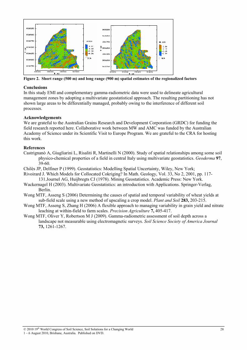
© 2010 19th World Congress of Soil Science, Soil Solutions for a Changing World
1 – 6 August 2010, Brisbane, Australia. Published on DVD. 28
Figure 2. Short range (500 m) and long range (900 m) spatial estimates of the regionalized factors
Conclusions In this study EMI and complementary gamma-radiometric data were used to delineate agricultural
management zones by adopting a multivariate geostatistical approach. The resulting partitioning has not
shown large areas to be differentially managed, probably owing to the interference of different soil
processes.
Acknowledgements We are grateful to the Australian Grains Research and Development Corporation (GRDC) for funding the
field research reported here. Collaborative work between MW and AMC was funded by the Australian
Academy of Science under its Scientific Visit to Europe Program. We are grateful to the CRA for hosting
this work.
References Castrignanò A, Giugliarini L, Risaliti R, Martinelli N (2000). Study of spatial relationships among some soil
physico-chemical properties of a field in central Italy using multivariate geostatistics. Geoderma 97,
39-60.
Chilès JP, Delfiner P (1999). Geostatistics: Modelling Spatial Uncertainty, Wiley, New York;
Rivoirard J. Which Models for Collocated Cokriging? In Math. Geology, Vol. 33, No 2, 2001, pp. 117-
131.Journel AG, Huijbregts CJ (1978). Mining Geostatistics. Academic Press: New York.
Wackernagel H (2003). Multivariate Geostatistics: an introduction with Applications. Springer-Verlag,
Berlin.
Wong MTF, Asseng S (2006) Determining the causes of spatial and temporal variability of wheat yields at
sub-field scale using a new method of upscaling a crop model. Plant and Soil 283, 203-215.
Wong MTF, Asseng S, Zhang H (2006) A flexible approach to managing variability in grain yield and nitrate
leaching at within-field to farm scales. Precision Agriculture 7, 405-417.
Wong MTF, Oliver Y, Robertson M J (2009). Gamma-radiometric assessment of soil depth across a
landscape not measurable using electromagnetic surveys. Soil Science Society of America Journal
73, 1261-1267.
© 2010 19th World Congress of Soil Science, Soil Solutions for a Changing World
1 – 6 August 2010, Brisbane, Australia. Published on DVD. 29
Can electromagnetic induction be used to evaluate sprinkler irrigation
uniformity for a shallow rooted crop?
Amjed HussainA and Steven R Raine
B
AScientist Hydrology, Future Farming Systems Research Division, Department of Primary Industries, Tatura, VIC 3616, Australia.
[email protected] BProfessor, National Centre for Engineering in Agriculture & CRC Irrigation Futures, University of Southern Queensland,
Toowoomba, QLD 4350, Australia. [email protected]
Abstract The application uniformity of sprinkler irrigation systems affects both crop growth and profitability.
However, traditional catch can measurements of irrigation uniformity are labour intensive and are normally
only conducted in a small area of the field. A trial was established in a lettuce crop irrigated with a solid set
sprinkler system to evaluate the potential to use electromagnetic sensing for irrigation performance
assessment. After crop establishment, the uniformity of the irrigation applications was deliberately modified
within two sprinkler plots (9 m x 11 m) by reducing the sprinkler operating pressures. The uniformity of the
water applied during each irrigation was measured using a grid of catch cans. The apparent soil electrical
conductivity (ECa) was measured within the plots for each irrigation during the cropping season using an
EM38. Electromagnetic (EM) measurements were taken with the EM38 either on the ground or 35 cm
above the ground surface. Elevating the EM sensor above the ground level did not improve the correlation
between the point measured catch can volume of water applied and the difference in ECa measured before
and after irrigation (∆ECa). However, the coefficient of uniformity calculated using the ∆ECa data was
correlated to the coefficient of uniformity calculated from the catch can data. The correlation was improved
where the EM sensor was elevated above the soil surface so that only the root zone was sensed. This
suggests that measurements of ∆ECa can be used to estimate the irrigation uniformity for shallow rooted
crops, particularly when the uniformity is low (CU < 70%) and the irrigation application pattern is consistent
throughout the season. ∆ECa measurements also identified the location of irrigation system leakages within
the field.
Key Words Apparent electrical conductivity, irrigation performance, leakage.
Introduction The uniformity of water application is a key performance measure of an irrigation system. As the uniformity
of water application decreases there is an increasing range of volumes applied within the irrigated area (Li
and Rao 2003) which may adversely affect crop growth and profitability (Barber and Raine 2002; Elms et al.
2001). Catch can measurements are commonly used to evaluate the spatial variability of water application.
However, discrete physical sampling can be labour intensive restricting the number of samples collected and
the ability to identify all spatial variability in the field (Plant 2001). Electromagnetic (EM) sensors have
been used to measure apparent (or bulk) soil electrical conductivity (ECa) and identify spatial variations in
soil moisture (Heiniger et al. 2003; Taylor et al. 2003). However, there are few reported studies using EM
sensing for evaluating irrigation uniformity, particularly where small volumes of water are applied using
sprinkler irrigation systems.
Hussain and Raine (2008) reported on a preliminary study using an EM sensor to evaluate the uniformity of
application for a sprinkler irrigated lettuce crop. ECa was found to be correlated with the seasonal pattern in
water application where the uniformity of water application was low and the spatial pattern of application
was consistent throughout the season. The ECa was not well correlated with the uniformity of individual
application events or where the irrigation uniformity was comparatively high. However, the EM sensor in
the preliminary study was placed on the soil surface resulting in the soil measurement depth being much
greater than the rooting depth of the crop, possibly reducing the ability of the instrument to resolve the small
volumes of water applied. Similarly, there was some uncertainty over the ability to correlate a point
measured catch can volume with an EM measurement averaged over a larger spatial area. Hence, this paper
reports on a subsequent field study to evaluate whether (a) elevating the EM sensor above the soil surface
improves the ability to identify spatial variations in small water applications and (b) correlations exist
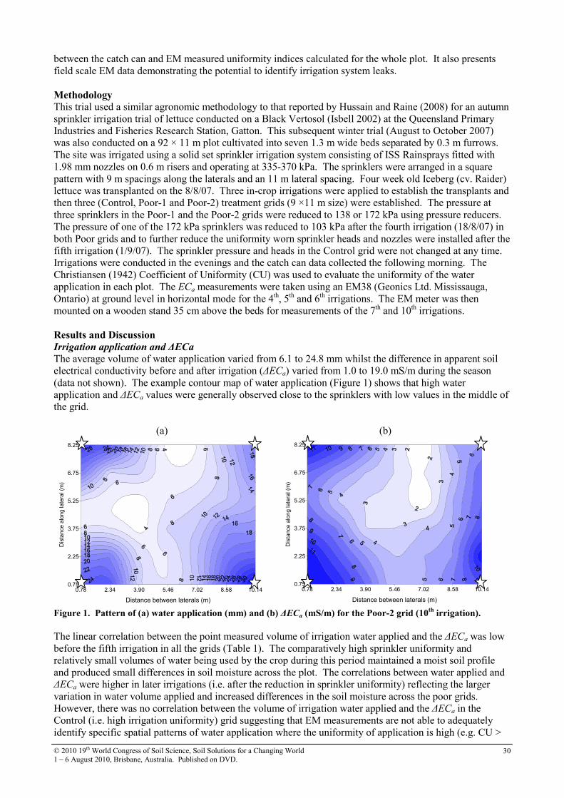
© 2010 19th World Congress of Soil Science, Soil Solutions for a Changing World
1 – 6 August 2010, Brisbane, Australia. Published on DVD. 30
between the catch can and EM measured uniformity indices calculated for the whole plot. It also presents
field scale EM data demonstrating the potential to identify irrigation system leaks.
Methodology This trial used a similar agronomic methodology to that reported by Hussain and Raine (2008) for an autumn
sprinkler irrigation trial of lettuce conducted on a Black Vertosol (Isbell 2002) at the Queensland Primary
Industries and Fisheries Research Station, Gatton. This subsequent winter trial (August to October 2007)
was also conducted on a 92 × 11 m plot cultivated into seven 1.3 m wide beds separated by 0.3 m furrows.
The site was irrigated using a solid set sprinkler irrigation system consisting of ISS Rainsprays fitted with
1.98 mm nozzles on 0.6 m risers and operating at 335-370 kPa. The sprinklers were arranged in a square
pattern with 9 m spacings along the laterals and an 11 m lateral spacing. Four week old Iceberg (cv. Raider)
lettuce was transplanted on the 8/8/07. Three in-crop irrigations were applied to establish the transplants and
then three (Control, Poor-1 and Poor-2) treatment grids (9 ×11 m size) were established. The pressure at
three sprinklers in the Poor-1 and the Poor-2 grids were reduced to 138 or 172 kPa using pressure reducers.
The pressure of one of the 172 kPa sprinklers was reduced to 103 kPa after the fourth irrigation (18/8/07) in
both Poor grids and to further reduce the uniformity worn sprinkler heads and nozzles were installed after the
fifth irrigation (1/9/07). The sprinkler pressure and heads in the Control grid were not changed at any time.
Irrigations were conducted in the evenings and the catch can data collected the following morning. The
Christiansen (1942) Coefficient of Uniformity (CU) was used to evaluate the uniformity of the water
application in each plot. The ECa measurements were taken using an EM38 (Geonics Ltd. Mississauga,
Ontario) at ground level in horizontal mode for the 4th, 5
th and 6
th irrigations. The EM meter was then
mounted on a wooden stand 35 cm above the beds for measurements of the 7th and 10
th irrigations.
Results and Discussion
Irrigation application and ∆ECa
The average volume of water application varied from 6.1 to 24.8 mm whilst the difference in apparent soil
electrical conductivity before and after irrigation (∆ECa) varied from 1.0 to 19.0 mS/m during the season
(data not shown). The example contour map of water application (Figure 1) shows that high water
application and ∆ECa values were generally observed close to the sprinklers with low values in the middle of
the grid.
(a) (b)
Figure 1. Pattern of (a) water application (mm) and (b) ∆ECa (mS/m) for the Poor-2 grid (10th
irrigation).
The linear correlation between the point measured volume of irrigation water applied and the ∆ECa was low
before the fifth irrigation in all the grids (Table 1). The comparatively high sprinkler uniformity and
relatively small volumes of water being used by the crop during this period maintained a moist soil profile
and produced small differences in soil moisture across the plot. The correlations between water applied and
∆ECa were higher in later irrigations (i.e. after the reduction in sprinkler uniformity) reflecting the larger
variation in water volume applied and increased differences in the soil moisture across the poor grids.
However, there was no correlation between the volume of irrigation water applied and the ∆ECa in the
Control (i.e. high irrigation uniformity) grid suggesting that EM measurements are not able to adequately
identify specific spatial patterns of water application where the uniformity of application is high (e.g. CU >
0.78 2.34 3.90 5.46 7.02 8.58 10.14
Distance between laterals (m)
0.75
2.25
3.75
5.25
6.75
8.25
Dis
tan
ce a
long
la
tera
l (m
)
0.78 2.34 3.90 5.46 7.02 8.58 10.14
Distance between laterals (m)
0.75
2.25
3.75
5.25
6.75
8.25
Dis
tance
alo
ng
late
ral (m
)
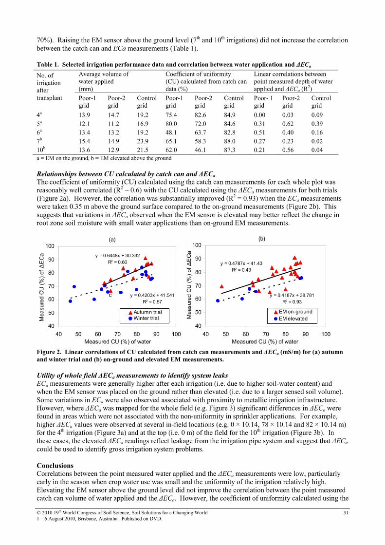
© 2010 19th World Congress of Soil Science, Soil Solutions for a Changing World
1 – 6 August 2010, Brisbane, Australia. Published on DVD. 31
70%). Raising the EM sensor above the ground level (7th and 10
th irrigations) did not increase the correlation
between the catch can and ECa measurements (Table 1).
Table 1. Selected irrigation performance data and correlation between water application and ∆ECa
Average volume of
water applied
(mm)
Coefficient of uniformity
(CU) calculated from catch can
data (%)
Linear correlations between
point measured depth of water
applied and ∆ECa (R2)
No. of
irrigation
after
transplant
Poor-1
grid
Poor-2
grid
Control
grid
Poor-1
grid
Poor-2
grid
Control
grid
Poor- 1
grid
Poor-2
grid
Control
grid
4a 13.9 14.7 19.2 75.4 82.6 84.9 0.00 0.03 0.09
5a 12.1 11.2 16.9 80.0 72.0 84.6 0.31 0.62 0.39
6a 13.4 13.2 19.2 48.1 63.7 82.8 0.51 0.40 0.16
7b 15.4 14.9 23.9 65.1 58.3 88.0 0.27 0.23 0.02
10b 13.6 12.9 21.5 62.0 46.1 87.3 0.21 0.56 0.04
a = EM on the ground, b = EM elevated above the ground
Relationships between CU calculated by catch can and ∆ECa
The coefficient of uniformity (CU) calculated using the catch can measurements for each whole plot was
reasonably well correlated (R2 ~ 0.6) with the CU calculated using the ∆ECa measurements for both trials
(Figure 2a). However, the correlation was substantially improved (R2 = 0.93) when the ECa measurements
were taken 0.35 m above the ground surface compared to the on-ground measurements (Figure 2b). This
suggests that variations in ∆ECa observed when the EM sensor is elevated may better reflect the change in
root zone soil moisture with small water applications than on-ground EM measurements.
(a)
y = 0.6448x + 30.332
R2 = 0.60
y = 0.4203x + 41.541
R2 = 0.57
40
50
60
70
80
90
100
40 50 60 70 80 90 100
Measured CU (%) of water
M
easure
d C
U (
%)
of
∆E
Ca
Autumn trialWinter trial
c
(b)
y = 0.4787x + 41.43
R2 = 0.43
y = 0.4187x + 38.781
R2 = 0.93
40
50
60
70
80
90
100
40 50 60 70 80 90 100
Measured CU (%) of water
Measure
d C
U (
%)
of
∆E
Ca
EM on-ground
EM elevated
Figure 2. Linear correlations of CU calculated from catch can measurements and ∆ECa (mS/m) for (a) autumn
and winter trial and (b) on-ground and elevated EM measurements.
Utility of whole field ∆ECa measurements to identify system leaks
ECa measurements were generally higher after each irrigation (i.e. due to higher soil-water content) and
when the EM sensor was placed on the ground rather than elevated (i.e. due to a larger sensed soil volume).
Some variations in ECa were also observed associated with proximity to metallic irrigation infrastructure.
However, where ∆ECa was mapped for the whole field (e.g. Figure 3) significant differences in ∆ECa were
found in areas which were not associated with the non-uniformity in sprinkler applications. For example,
higher ∆ECa values were observed at several in-field locations (e.g. 0 × 10.14, 78 × 10.14 and 82 × 10.14 m)
for the 4th irrigation (Figure 3a) and at the top (i.e. 0 m) of the field for the 10
th irrigation (Figure 3b). In
these cases, the elevated ∆ECa readings reflect leakage from the irrigation pipe system and suggest that ∆ECa
could be used to identify gross irrigation system problems.
Conclusions Correlations between the point measured water applied and the ∆ECa measurements were low, particularly
early in the season when crop water use was small and the uniformity of the irrigation relatively high.
Elevating the EM sensor above the ground level did not improve the correlation between the point measured
catch can volume of water applied and the ∆ECa. However, the coefficient of uniformity calculated using the
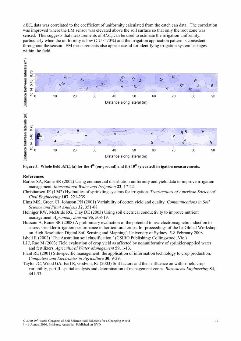
© 2010 19th World Congress of Soil Science, Soil Solutions for a Changing World
1 – 6 August 2010, Brisbane, Australia. Published on DVD. 32
∆ECa data was correlated to the coefficient of uniformity calculated from the catch can data. The correlation
was improved where the EM sensor was elevated above the soil surface so that only the root zone was
sensed. This suggests that measurements of ∆ECa can be used to estimate the irrigation uniformity,
particularly when the uniformity is low (CU < 70%) and the irrigation application pattern is consistent
throughout the season. EM measurements also appear useful for identifying irrigation system leakages
within the field.
0.7
85.4
610.1
4
Dis
tance
be
twee
n late
rals
(m
)
0 10 20 30 40 50 60 70 80 90
Distance along lateral (m)
0.7
85.4
610.1
4
Dis
tance
betw
een late
rals
(m
)
0 10 20 30 40 50 60 70 80 90
Distance along lateral (m)
Figure 3. Whole field ∆ECa (a) for the 4th
(on-ground) and (b) 10th
(elevated) irrigation measurements.
References Barber SA, Raine SR (2002) Using commercial distribution uniformity and yield data to improve irrigation
management. International Water and Irrigation 22, 17-22.
Christiansen JE (1942) Hydraulics of sprinkling systems for irrigation. Transactions of American Society of
Civil Engineering 107, 221-239.
Elms MK, Green CJ, Johnson PN (2001) Variability of cotton yield and quality. Communications in Soil
Science and Plant Analysis 32, 351-68.
Heiniger RW, McBride RG, Clay DE (2003) Using soil electrical conductivity to improve nutrient
management. Agronomy Journal 95, 508-19.
Hussain A, Raine SR (2008) A preliminary evaluation of the potential to use electromagnetic induction to
assess sprinkler irrigation performance in horticultural crops. In ‘proceedings of the Ist Global Workshop
on High Resolution Digital Soil Sensing and Mapping’. University of Sydney, 5-8 February 2008.
Isbell R (2002) ‘The Australian soil classification.’ (CSIRO Publishing: Collingwood, Vic.)
Li J, Rao M (2003) Field evaluation of crop yield as affected by nonuniformity of sprinkler-applied water
and fertilizers. Agricultural Water Management 59, 1-13.
Plant RE (2001) Site-specific management: the application of information technology to crop production.
Computers and Electronics in Agriculture 30, 9-29.
Taylor JC, Wood GA, Earl R, Godwin, RJ (2003) Soil factors and their influence on within-field crop
variability, part II: spatial analysis and determination of management zones. Biosystems Engineering 84,
441-53.

© 2010 19th World Congress of Soil Science, Soil Solutions for a Changing World
1 – 6 August 2010, Brisbane, Australia. Published on DVD. 33
Can field-based spectroscopic sensors measure soil carbon in a regulated carbon
trading program?
Eric D. Lund Veris Technologies, Inc., Salina KS USA, www.veristech.com
Abstract Measuring changes in soil carbon is a daunting task, as soil carbon levels can vary significantly at short distances.
Uncertainty about soil carbon measurements is affecting agriculture’s consideration as an offset provider under a
regulated greenhouse gas program, such as cap-and-trade. Purchasers of carbon offsets must be assured that carbon
changes are real, and not just an artifact of sampling locations. To complicate matters further, measurements must
include the soil profile, making this a three-dimensional effort. Veris Technologies has developed a system that
employs a suite of sensors, including near-infrared spectroscopy, to measure carbon throughout the soil profile. The
system was deployed on a set of nine fields in Kansas USA, with the objective of establishing a baseline soil carbon
inventory. Lab-analyzed soil samples were used to calibrate and cross-validate the field sensors, and confidence
intervals from sensors and lab were compared.
Key Words near-infrared, spatial variability, cap-and-trade, spectrometer, soil electrical conductivity
Introduction Since 1850, soils have lost an estimated 78 Gt of carbon, primarily due to cultivation (Lal 2009). This loss of
soil carbon represents a significant portion of greenhouse gas emissions, and has resulted in the degradation
of agricultural soil quality worldwide. Using practices that restore carbon, such as no-till farming, carbon can
be sequestered in the soil. Carbon sequestration has the potential to offset fossil fuel emissions by 0.4 to 1.2
gigatons of carbon per year, or 5 to 15% of the global fossil-fuel emissions (Lal 2004).
Under a carbon trading system, farmers and landowners would be paid for adopting carbon-sequestration
techniques, provided their increases in carbon can be measured, monitored and verified. Accounting for soil
carbon changes is difficult, because carbon increases due to farming practice changes are very small, and
carbon varies widely within a field, even within a few meters. What causes soil carbon spatial variability?
In addition to the macro factors such as soil formation, soil type, and historical land use, there are many
micro-scale influences: crop residues are distributed unevenly from combine harvesters, heavy rains remove
and deposit piles of residue sporadically, animals defecate and die in random locations, and many other
factors add variations.
In order to verify that carbon has been sequestered, a baseline must be established at the beginning of the
project, along with subsequent measuring to verify the carbon change. The amount of carbon that is
accredited will be based on the confidence, likely at the 90% level, of those measurements (Willey and
Chameides 2007). The confidence interval is determined by the number of samples and the variability of the
carbon. If the standard deviation is large, additional samples are required to reduce the confidence interval.
If the sampling rate is insufficient, the carbon payment discount due to the uncertainty will be large. If an
adequate number of samples are collected, the cost of conventional soil sampling and lab-analysis could be
excessive. An alternative that generates large numbers of carbon analyses at a very low cost per sample must
be considered. Near-infrared reflectance (NIR) spectroscopy has been shown to correlate well with soil
carbon (Sudduth and Hummel 1993; Reeves et al. 1999; Shepherd and Walsh 2002). NIR spectroscopy and
other proximal field sensors were tested in a soil carbon project on a set of nine fields in northeast Kansas.
The objective for this project was to establish baseline soil carbon measurements on land that is currently
under contract to produce greenhouse gas reduction and offsets. These measurements were intended to
provide quality assurance of the initial carbon levels for the greenhouse gas offsets that will be produced on
these lands, and to generate information about costs of carbon quantification.
Materials and Methods A commercially available system from Veris Technologies that maps the surface and the soil profile to a
depth of one meter was used on this project. The system is comprised of two modules: an on-the-go shank
for collecting measurements at a discrete depth as it maps transects across a field (Figure 1), and a probe for
collecting measurements of the soil profile to a depth of one meter (Figure 2). Both modules collect visible
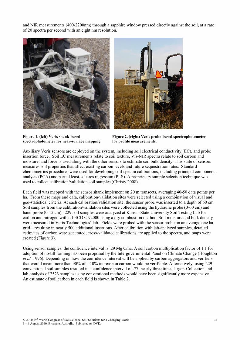
© 2010 19th World Congress of Soil Science, Soil Solutions for a Changing World
1 – 6 August 2010, Brisbane, Australia. Published on DVD. 34
and NIR measurements (400-2200nm) through a sapphire window pressed directly against the soil, at a rate
of 20 spectra per second with an eight nm resolution.
Figure 1. (left) Veris shank-based
spectrophotometer for near-surface mapping.
Figure 2. (right) Veris probe-based spectrophotometer
for profile measurements.
Auxiliary Veris sensors are deployed on the system, including soil electrical conductivity (EC), and probe
insertion force. Soil EC measurements relate to soil texture, Vis-NIR spectra relate to soil carbon and
moisture, and force is used along with the other sensors to estimate soil bulk density. This suite of sensors
measures soil properties that affect existing carbon levels and future sequestration rates. Standard
chemometrics procedures were used for developing soil-spectra calibrations, including principal components
analysis (PCA) and partial least-squares regression (PLS). A proprietary sample selection technique was
used to collect calibration/validation soil samples (Christy 2008).
Each field was mapped with the sensor shank implement on 20 m transects, averaging 40-50 data points per
ha. From these maps and data, calibration/validation sites were selected using a combination of visual and
geo-statistical criteria. At each calibration/validation site, the sensor probe was inserted to a depth of 60 cm.
Soil samples from the calibration/validation sites were collected using the hydraulic probe (0-60 cm) and
hand probe (0-15 cm). 229 soil samples were analyzed at Kansas State University Soil Testing Lab for
carbon and nitrogen with a LECO CN2000 using a dry combustion method. Soil moisture and bulk density
were measured in Veris Technologies’ lab. Fields were probed with the sensor probe on an average one ha
grid—resulting in nearly 500 additional insertions. After calibration with lab-analyzed samples, detailed
estimates of carbon were generated, cross-validated calibrations are applied to the spectra, and maps were
created (Figure 3).
Using sensor samples, the confidence interval is .29 Mg C/ha. A soil carbon multiplication factor of 1.1 for
adoption of no-till farming has been proposed by the Intergovernmental Panel on Climate Change (Houghton
et al. 1996). Depending on how the confidence interval will be applied by carbon aggregators and verifiers,
that would mean more than 90% of a 10% increase in carbon would be verifiable. Alternatively, using 229
conventional soil samples resulted in a confidence interval of .77, nearly three times larger. Collection and
lab-analysis of 2523 samples using conventional methods would have been significantly more expensive.
An estimate of soil carbon in each field is shown in Table 2.
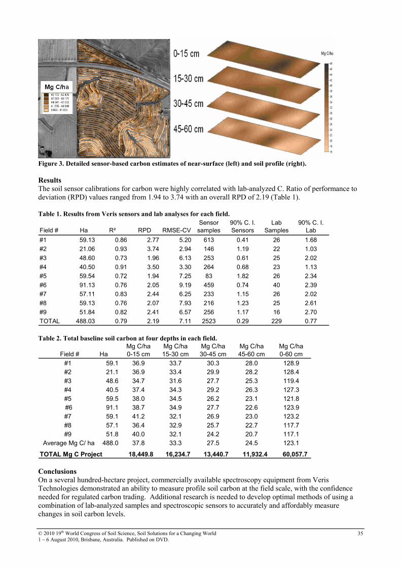
© 2010 19th World Congress of Soil Science, Soil Solutions for a Changing World
1 – 6 August 2010, Brisbane, Australia. Published on DVD. 35
Figure 3. Detailed sensor-based carbon estimates of near-surface (left) and soil profile (right).
Results The soil sensor calibrations for carbon were highly correlated with lab-analyzed C. Ratio of performance to
deviation (RPD) values ranged from 1.94 to 3.74 with an overall RPD of 2.19 (Table 1).
Table 1. Results from Veris sensors and lab analyses for each field.
Table 2. Total baseline soil carbon at four depths in each field.
Conclusions On a several hundred-hectare project, commercially available spectroscopy equipment from Veris
Technologies demonstrated an ability to measure profile soil carbon at the field scale, with the confidence
needed for regulated carbon trading. Additional research is needed to develop optimal methods of using a
combination of lab-analyzed samples and spectroscopic sensors to accurately and affordably measure
changes in soil carbon levels.
Field # Ha R² RPD RMSE-CV
Sensor
samples
90% C. I.
Sensors
Lab
Samples
90% C. I.
Lab
#1 59.13 0.86 2.77 5.20 613 0.41 26 1.68
#2 21.06 0.93 3.74 2.94 146 1.19 22 1.03
#3 48.60 0.73 1.96 6.13 253 0.61 25 2.02
#4 40.50 0.91 3.50 3.30 264 0.68 23 1.13
#5 59.54 0.72 1.94 7.25 83 1.82 26 2.34
#6 91.13 0.76 2.05 9.19 459 0.74 40 2.39
#7 57.11 0.83 2.44 6.25 233 1.15 26 2.02
#8 59.13 0.76 2.07 7.93 216 1.23 25 2.61
#9 51.84 0.82 2.41 6.57 256 1.17 16 2.70
TOTAL 488.03 0.79 2.19 7.11 2523 0.29 229 0.77
Field # Ha
Mg C/ha
0-15 cm
Mg C/ha
15-30 cm
Mg C/ha
30-45 cm
Mg C/ha
45-60 cm
Mg C/ha
0-60 cm
#1 59.1 36.9 33.7 30.3 28.0 128.9
#2 21.1 36.9 33.4 29.9 28.2 128.4
#3 48.6 34.7 31.6 27.7 25.3 119.4
#4 40.5 37.4 34.3 29.2 26.3 127.3
#5 59.5 38.0 34.5 26.2 23.1 121.8
#6 91.1 38.7 34.9 27.7 22.6 123.9
#7 59.1 41.2 32.1 26.9 23.0 123.2
#8 57.1 36.4 32.9 25.7 22.7 117.7
#9 51.8 40.0 32.1 24.2 20.7 117.1
Average Mg C/ ha 488.0 37.8 33.3 27.5 24.5 123.1
TOTAL Mg C Project 18,449.8 16,234.7 13,440.7 11,932.4 60,057.7

© 2010 19th World Congress of Soil Science, Soil Solutions for a Changing World
1 – 6 August 2010, Brisbane, Australia. Published on DVD. 36
References Christy CD (2008) Real-time measurement of soil attributes using on-the-go near infrared reflectance
spectroscopy. Computers and Electronics in Agriculture 61(1), 10-19.
Houghton JT, Meira Filho LG, Lim B, Treanton K, Imamaty I (1996) IPCC Guidelines for National
Greenhouse Gas Inventories. Volumes 1–3. Hadley Centre Meteorological Office, United Kingdom.
Lal R (2004) Soil carbon sequestration impacts on global climate change and food security. Science
304(5677), 1623-1627.
Lal R (2009) Challenges and opportunities in soil organic matter research. European Journal of Soil Science
60, 158-169.
Reeves JB, McCarty GW, Meisinger JJ (1999) Near infrared reflectance spectroscopy for the analysis of
agricultural soils. Journal of Near Infrared Spectroscopy 9(1), 25-34.
Shepherd KD, Walsh MG (2002) Development of reflectance spectral libraries for characterization of soil
properties. Soil Science Society of America Journal 66, 988-998.
Sudduth KA, Hummel JW (1993) Portable, near-infrared spectrophotometer for rapid soil analysis.
Transactions of the ASAE 36, 185-193.
Willey Z, Chameides B (2007) Harnessing farms and forests in the low-carbon economy—how to create,
measure, and verify greenhouse gas offsets. pp. 118-124 Duke University Press.
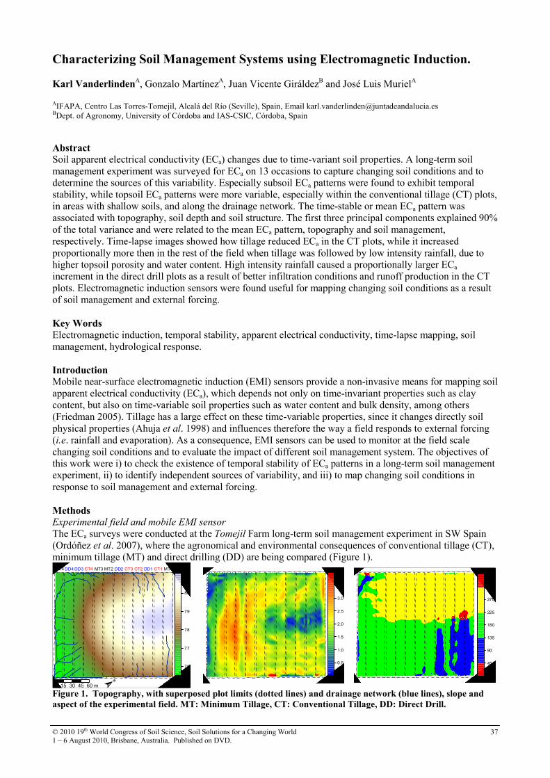
© 2010 19th World Congress of Soil Science, Soil Solutions for a Changing World
1 – 6 August 2010, Brisbane, Australia. Published on DVD. 37
Characterizing Soil Management Systems using Electromagnetic Induction.
Karl VanderlindenA, Gonzalo Martínez
A, Juan Vicente Giráldez
B and José Luis Muriel
A
AIFAPA, Centro Las Torres-Tomejil, Alcalá del Río (Seville), Spain, Email [email protected] BDept. of Agronomy, University of Córdoba and IAS-CSIC, Córdoba, Spain
Abstract Soil apparent electrical conductivity (ECa) changes due to time-variant soil properties. A long-term soil
management experiment was surveyed for ECa on 13 occasions to capture changing soil conditions and to
determine the sources of this variability. Especially subsoil ECa patterns were found to exhibit temporal
stability, while topsoil ECa patterns were more variable, especially within the conventional tillage (CT) plots,
in areas with shallow soils, and along the drainage network. The time-stable or mean ECa pattern was
associated with topography, soil depth and soil structure. The first three principal components explained 90%
of the total variance and were related to the mean ECa pattern, topography and soil management,
respectively. Time-lapse images showed how tillage reduced ECa in the CT plots, while it increased
proportionally more then in the rest of the field when tillage was followed by low intensity rainfall, due to
higher topsoil porosity and water content. High intensity rainfall caused a proportionally larger ECa
increment in the direct drill plots as a result of better infiltration conditions and runoff production in the CT
plots. Electromagnetic induction sensors were found useful for mapping changing soil conditions as a result
of soil management and external forcing.
Key Words Electromagnetic induction, temporal stability, apparent electrical conductivity, time-lapse mapping, soil
management, hydrological response.
Introduction Mobile near-surface electromagnetic induction (EMI) sensors provide a non-invasive means for mapping soil
apparent electrical conductivity (ECa), which depends not only on time-invariant properties such as clay
content, but also on time-variable soil properties such as water content and bulk density, among others
(Friedman 2005). Tillage has a large effect on these time-variable properties, since it changes directly soil
physical properties (Ahuja et al. 1998) and influences therefore the way a field responds to external forcing
(i.e. rainfall and evaporation). As a consequence, EMI sensors can be used to monitor at the field scale
changing soil conditions and to evaluate the impact of different soil management system. The objectives of
this work were i) to check the existence of temporal stability of ECa patterns in a long-term soil management
experiment, ii) to identify independent sources of variability, and iii) to map changing soil conditions in
response to soil management and external forcing.
Methods Experimental field and mobile EMI sensor
The ECa surveys were conducted at the Tomejil Farm long-term soil management experiment in SW Spain
(Ordóñez et al. 2007), where the agronomical and environmental consequences of conventional tillage (CT),
minimum tillage (MT) and direct drilling (DD) are being compared (Figure 1).
76
77
78
79
80
81
m.a.s.l.
MT1CT1CT2 DD1CT3CT4 MT2MT3MT4 DD2DD3DD4
0 15 30 45 60 m 0.0
0.5
1.0
1.5
2.0
2.5
3.0
3.5
4.0
slope (º) 0
45
90
135
180
225
270
315
360
aspect (º)
Figure 1. Topography, with superposed plot limits (dotted lines) and drainage network (blue lines), slope and
aspect of the experimental field. MT: Minimum Tillage, CT: Conventional Tillage, DD: Direct Drill.
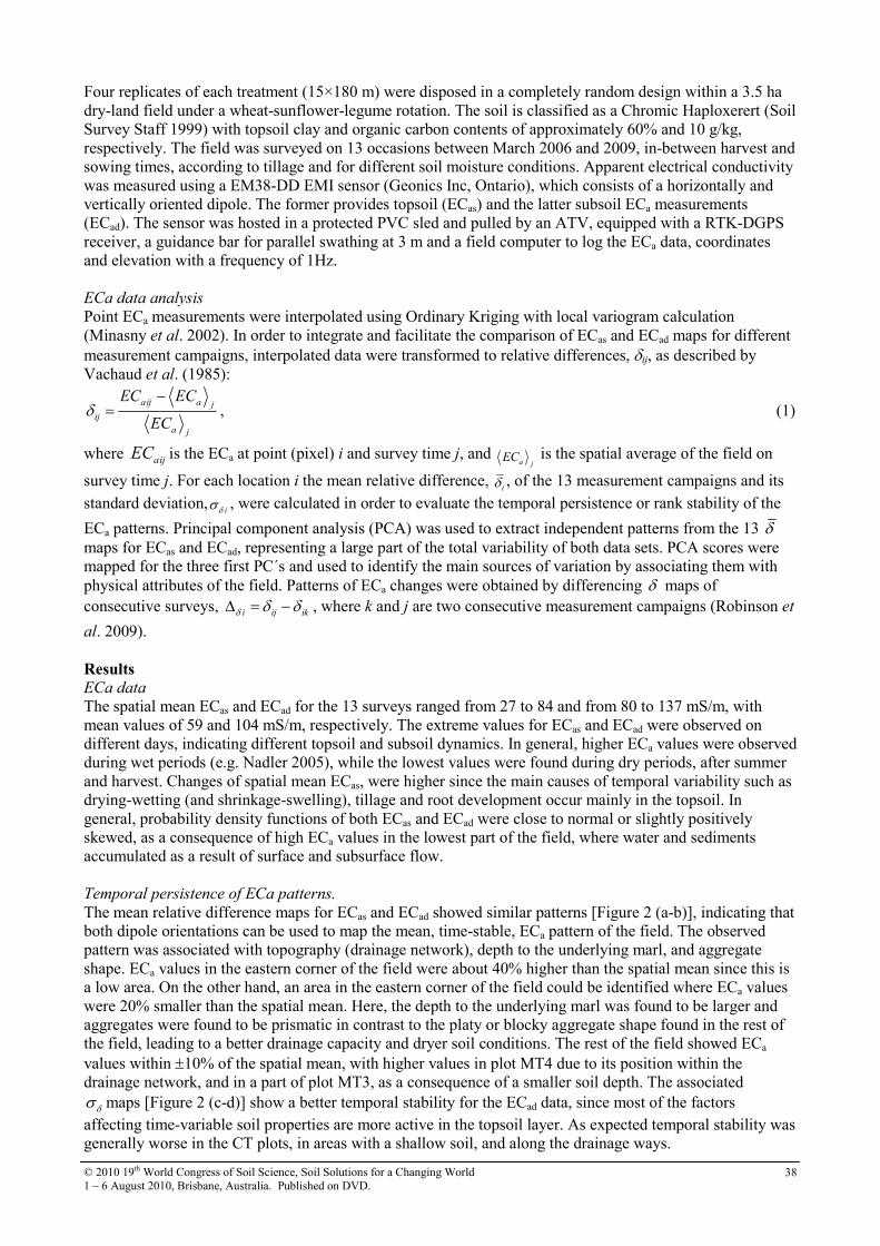
© 2010 19th World Congress of Soil Science, Soil Solutions for a Changing World
1 – 6 August 2010, Brisbane, Australia. Published on DVD. 38
Four replicates of each treatment (15×180 m) were disposed in a completely random design within a 3.5 ha
dry-land field under a wheat-sunflower-legume rotation. The soil is classified as a Chromic Haploxerert (Soil
Survey Staff 1999) with topsoil clay and organic carbon contents of approximately 60% and 10 g/kg,
respectively. The field was surveyed on 13 occasions between March 2006 and 2009, in-between harvest and
sowing times, according to tillage and for different soil moisture conditions. Apparent electrical conductivity
was measured using a EM38-DD EMI sensor (Geonics Inc, Ontario), which consists of a horizontally and
vertically oriented dipole. The former provides topsoil (ECas) and the latter subsoil ECa measurements
(ECad). The sensor was hosted in a protected PVC sled and pulled by an ATV, equipped with a RTK-DGPS
receiver, a guidance bar for parallel swathing at 3 m and a field computer to log the ECa data, coordinates
and elevation with a frequency of 1Hz.
ECa data analysis
Point ECa measurements were interpolated using Ordinary Kriging with local variogram calculation
(Minasny et al. 2002). In order to integrate and facilitate the comparison of ECas and ECad maps for different
measurement campaigns, interpolated data were transformed to relative differences, δij, as described by
Vachaud et al. (1985):
aij a j
ij
a j
EC EC
ECδ
−= , (1)
where aijEC is the ECa at point (pixel) i and survey time j, and a j
EC is the spatial average of the field on
survey time j. For each location i the mean relative difference, iδ , of the 13 measurement campaigns and its
standard deviation,iδσ , were calculated in order to evaluate the temporal persistence or rank stability of the
ECa patterns. Principal component analysis (PCA) was used to extract independent patterns from the 13 δ
maps for ECas and ECad, representing a large part of the total variability of both data sets. PCA scores were
mapped for the three first PC´s and used to identify the main sources of variation by associating them with
physical attributes of the field. Patterns of ECa changes were obtained by differencing δ maps of
consecutive surveys, i ij ikδ δ δ∆ = − , where k and j are two consecutive measurement campaigns (Robinson et
al. 2009).
Results ECa data
The spatial mean ECas and ECad for the 13 surveys ranged from 27 to 84 and from 80 to 137 mS/m, with
mean values of 59 and 104 mS/m, respectively. The extreme values for ECas and ECad were observed on
different days, indicating different topsoil and subsoil dynamics. In general, higher ECa values were observed
during wet periods (e.g. Nadler 2005), while the lowest values were found during dry periods, after summer
and harvest. Changes of spatial mean ECas, were higher since the main causes of temporal variability such as
drying-wetting (and shrinkage-swelling), tillage and root development occur mainly in the topsoil. In
general, probability density functions of both ECas and ECad were close to normal or slightly positively
skewed, as a consequence of high ECa values in the lowest part of the field, where water and sediments
accumulated as a result of surface and subsurface flow.
Temporal persistence of ECa patterns.
The mean relative difference maps for ECas and ECad showed similar patterns [Figure 2 (a-b)], indicating that
both dipole orientations can be used to map the mean, time-stable, ECa pattern of the field. The observed
pattern was associated with topography (drainage network), depth to the underlying marl, and aggregate
shape. ECa values in the eastern corner of the field were about 40% higher than the spatial mean since this is
a low area. On the other hand, an area in the eastern corner of the field could be identified where ECa values
were 20% smaller than the spatial mean. Here, the depth to the underlying marl was found to be larger and
aggregates were found to be prismatic in contrast to the platy or blocky aggregate shape found in the rest of
the field, leading to a better drainage capacity and dryer soil conditions. The rest of the field showed ECa
values within ±10% of the spatial mean, with higher values in plot MT4 due to its position within the
drainage network, and in a part of plot MT3, as a consequence of a smaller soil depth. The associated
δσ maps [Figure 2 (c-d)] show a better temporal stability for the ECad data, since most of the factors
affecting time-variable soil properties are more active in the topsoil layer. As expected temporal stability was
generally worse in the CT plots, in areas with a shallow soil, and along the drainage ways.
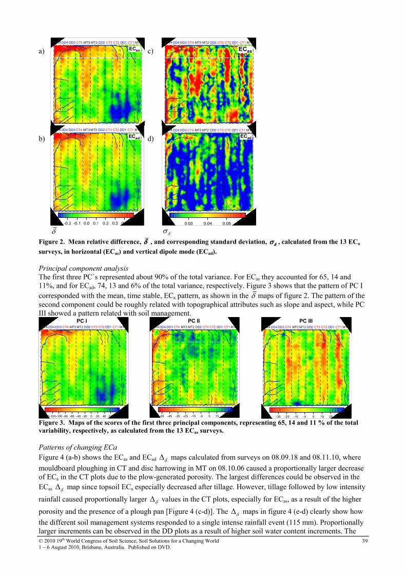
© 2010 19th World Congress of Soil Science, Soil Solutions for a Changing World
1 – 6 August 2010, Brisbane, Australia. Published on DVD. 39
a)
MT1CT1CT2 DD1CT3CT4 MT2MT3MT4 DD2DD3DD4
ECas
c) ECas
MT1CT1CT2 DD1CT3CT4 MT2MT3MT4 DD2DD3DD4
b)
-0.3 -0.2 -0.1 0.0 0.1 0.2 0.3 0.4 0.5
MT1CT1CT2 DD1CT3CT4 MT2MT3MT4 DD2DD3DD4
ECad
d)
0.02 0.03 0.04 0.05 0.06
MT1CT1CT2 DD1CT3CT4 MT2MT3MT4 DD2DD3DD4
ECad
δ
δσ
Figure 2. Mean relative difference, δδδδ , and corresponding standard deviation, δδδδσσσσ , calculated from the 13 ECa
surveys, in horizontal (ECas) and vertical dipole mode (ECad).
Principal component analysis
The first three PC´s represented about 90% of the total variance. For ECas they accounted for 65, 14 and
11%, and for ECad, 74, 13 and 6% of the total variance, respectively. Figure 3 shows that the pattern of PC I
corresponded with the mean, time stable, ECa pattern, as shown in the δ maps of figure 2. The pattern of the
second component could be roughly related with topographical attributes such as slope and aspect, while PC
III showed a pattern related with soil management.
-140-120-100 -80 -60 -40 -20 0 20 40 60 80
MT1CT1CT2 DD1CT3CT4 MT2MT3MT4 DD2DD3DD4
PC I
-55 -45 -35 -25 -15 -5 5 15 25
MT1CT1CT2 DD1CT3CT4 MT2MT3MT4 DD2DD3DD4
PC II
-35 -25 -15 -5 5 15 25
MT1CT1CT2 DD1CT3CT4 MT2MT3MT4 DD2DD3DD4
PC III
Figure 3. Maps of the scores of the first three principal components, representing 65, 14 and 11 % of the total
variability, respectively, as calculated from the 13 ECas surveys.
Patterns of changing ECa
Figure 4 (a-b) shows the ECas and ECad δ∆ maps calculated from surveys on 08.09.18 and 08.11.10, where
mouldboard ploughing in CT and disc harrowing in MT on 08.10.06 caused a proportionally larger decrease
of ECa in the CT plots due to the plow-generated porosity. The largest differences could be observed in the
ECas δ∆ map since topsoil ECa especially decreased after tillage. However, tillage followed by low intensity
rainfall caused proportionally larger δ∆ values in the CT plots, especially for ECas, as a result of the higher
porosity and the presence of a plough pan [Figure 4 (c-d)]. The δ∆ maps in figure 4 (e-d) clearly show how
the different soil management systems responded to a single intense rainfall event (115 mm). Proportionally
larger increments can be observed in the DD plots as a result of higher soil water content increments. The
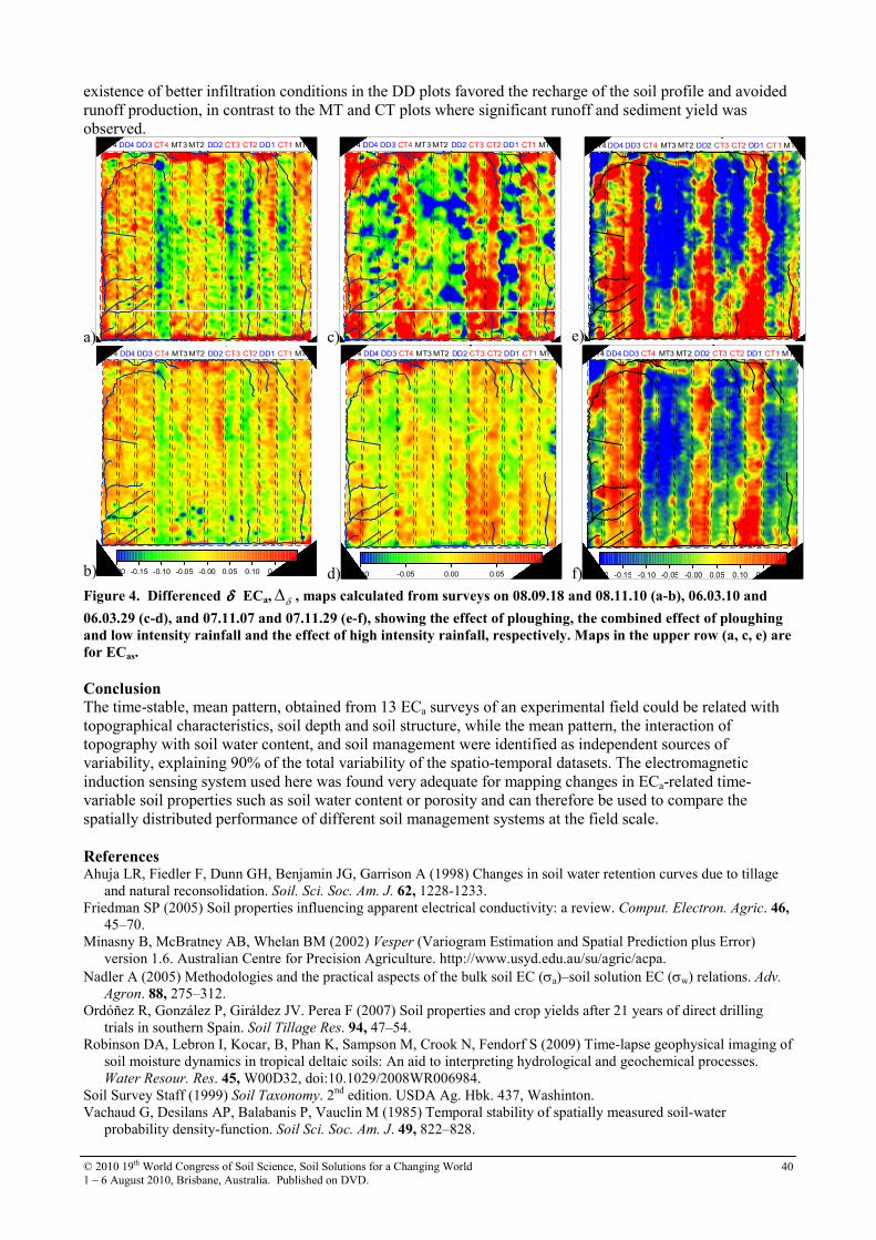
© 2010 19th World Congress of Soil Science, Soil Solutions for a Changing World
1 – 6 August 2010, Brisbane, Australia. Published on DVD. 40
existence of better infiltration conditions in the DD plots favored the recharge of the soil profile and avoided
runoff production, in contrast to the MT and CT plots where significant runoff and sediment yield was
observed.
a)
MT1CT1CT2 DD1CT3CT4 MT2MT3MT4 DD2DD3DD4
Horizontal dipole
c)
MT1CT1CT2 DD1CT3CT4 MT2MT3MT4 DD2DD3DD4
Horizontal dipole
e)
MT1CT1CT2 DD1CT3CT4 MT2MT3MT4 DD2DD3DD4
Horizontal dipole
b) -0.20 -0.15 -0.10 -0.05 -0.00 0.05 0.10 0.15 0.20
MT1CT1CT2 DD1CT3CT4 MT2MT3MT4 DD2DD3DD4
Vertical dipole
d) -0.10 -0.05 0.00 0.05 0.10
MT1CT1CT2 DD1CT3CT4 MT2MT3MT4 DD2DD3DD4
Vertical dipole
f)
MT1CT1CT2 DD1CT3CT4 MT2MT3MT4 DD2DD3DD4
-0.20 -0.15 -0.10 -0.05 -0.00 0.05 0.10 0.15 0.20
Vertical dipole
Figure 4. Differenced δδδδ ECa, δ∆ , maps calculated from surveys on 08.09.18 and 08.11.10 (a-b), 06.03.10 and
06.03.29 (c-d), and 07.11.07 and 07.11.29 (e-f), showing the effect of ploughing, the combined effect of ploughing
and low intensity rainfall and the effect of high intensity rainfall, respectively. Maps in the upper row (a, c, e) are
for ECas.
Conclusion The time-stable, mean pattern, obtained from 13 ECa surveys of an experimental field could be related with
topographical characteristics, soil depth and soil structure, while the mean pattern, the interaction of
topography with soil water content, and soil management were identified as independent sources of
variability, explaining 90% of the total variability of the spatio-temporal datasets. The electromagnetic
induction sensing system used here was found very adequate for mapping changes in ECa-related time-
variable soil properties such as soil water content or porosity and can therefore be used to compare the
spatially distributed performance of different soil management systems at the field scale.
References Ahuja LR, Fiedler F, Dunn GH, Benjamin JG, Garrison A (1998) Changes in soil water retention curves due to tillage
and natural reconsolidation. Soil. Sci. Soc. Am. J. 62, 1228-1233.
Friedman SP (2005) Soil properties influencing apparent electrical conductivity: a review. Comput. Electron. Agric. 46,
45–70.
Minasny B, McBratney AB, Whelan BM (2002) Vesper (Variogram Estimation and Spatial Prediction plus Error)
version 1.6. Australian Centre for Precision Agriculture. http://www.usyd.edu.au/su/agric/acpa.
Nadler A (2005) Methodologies and the practical aspects of the bulk soil EC (σa)–soil solution EC (σw) relations. Adv.
Agron. 88, 275–312.
Ordóñez R, González P, Giráldez JV. Perea F (2007) Soil properties and crop yields after 21 years of direct drilling
trials in southern Spain. Soil Tillage Res. 94, 47–54.
Robinson DA, Lebron I, Kocar, B, Phan K, Sampson M, Crook N, Fendorf S (2009) Time-lapse geophysical imaging of
soil moisture dynamics in tropical deltaic soils: An aid to interpreting hydrological and geochemical processes.
Water Resour. Res. 45, W00D32, doi:10.1029/2008WR006984.
Soil Survey Staff (1999) Soil Taxonomy. 2nd
edition. USDA Ag. Hbk. 437, Washinton.
Vachaud G, Desilans AP, Balabanis P, Vauclin M (1985) Temporal stability of spatially measured soil-water
probability density-function. Soil Sci. Soc. Am. J. 49, 822–828.
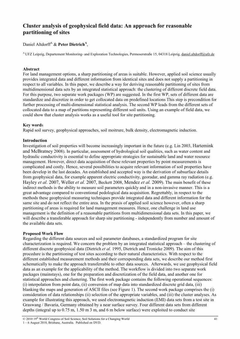
© 2010 19th World Congress of Soil Science, Soil Solutions for a Changing World
1 – 6 August 2010, Brisbane, Australia. Published on DVD. 41
Cluster analysis of geophysical field data: An approach for reasonable
partitioning of sites
Daniel Altdorff
A & Peter Dietrich
A,
A UFZ Leipzig, Departement Monitoring- and Exploration Technologies, Permoserstraße 15, 04318 Leipzig, [email protected]
Abstract For land management options, a sharp partitioning of areas is suitable. However, applied soil science usually
provides integrated data and different information from identical sites and does not supply a partitioning in
respect to all variables. In this paper, we describe a way for deriving reasonable partitioning of sites from
multidimensional data sets by an integrated statistical approach: the clustering of different discrete field data.
For this purpose, two separate work packages (WP) are suggested. In the first WP, sets of different data are
standardize and discretize in order to get collocated data on predefined locations This step is precondition for
further processing of multi-dimensional statistical analysis. The second WP leads from the different sets of
collocated data to a map of partitions representing different soil units. Using an example of field data, we
could show that cluster analysis works as a useful tool for site partitioning.
Key words
Rapid soil survey, geophysical approaches, soil moitrure, bulk density, electromagnetic induction.
Introduction
Investigation of soil properties will become increasingly important in the future (e.g. Lin 2003, Hartemink
and McBratney 2008). In particular, assessment of hydrological soil qualities, such as water content and
hydraulic conductivity is essential to define appropriate strategies for sustainable land and water resource
management. However, direct data acquisition of these relevant properties by point measurements is
complicated and costly. Hence, several possibilities to acquire relevant information of soil properties have
been develop in the last decades. An established and accepted way is the derivation of subsurface details
from geophysical data, for example apparent electric conductivity, georadar, and gamma ray radiation (e.g.
Hayley et al. 2007, Weller et al. 2007, Beckett 2008, Mendez et al. 2009). The main benefit of these
indirect methods is the ability to measure soil parameters quickly and in a non-invasive manner. This is a
great advantage compared to conventional pedological data acquisition. Regrettably, in respect to the
methods these geophysical measuring techniques provide integrated data and different information for the
same site and do not reflect the entire area. In the praxis of applied soil science however, often a sharp
partitioning of areas is required for land management measures. Hence, one challenge in land use
management is the definition of a reasonable partitions from multidimensional data sets. In this paper, we
will describe a transferable approach for sharp site partitioning - independently from number and amount of
the available data sets.
Proposed Work Flow Regarding the different data sources and soil parameter databases, a standardized program for site
characterization is required. We concern the problem by an integrated statistical approach – the clustering of
different discrete geophysical data (Dietrich et al. 1995, Dietrich and Tronicke 2009). The aim of this
procedure is the partitioning of test sites according to their natural characteristics. With respect to the
different established measurement methods and their corresponding data sets, we describe our method first
schematically to make the approach transferrable to other data sources. Afterwards, we use geophysical field
data as an example for the applicability of the method. The workflow is divided into two separate work
packages (mainstays), one for the preparation and discretization of the field data, and another one for
statistical approaches and clustering. The first work package contains the following operational sequences:
(i) interpolation from point data, (ii) conversion of map data into standardized discrete grid data, (iii)
blanking the maps and generation of ASCII files (see Figure 1). The second work package comprises the (i)
consideration of data relationships (ii) selection of the appropriate variables, and (iii) the cluster analyses. As
example for illustrating this approach, we used electromagnetic induction (EMI) data sets from a test site in
Graswang / Bavaria, Germany obtained by a near surface survey. Four different data sets from different
depths (integral up to 0.75 m, 1.50 m 3 m, and 6 m below surface) were exploited to conduct site
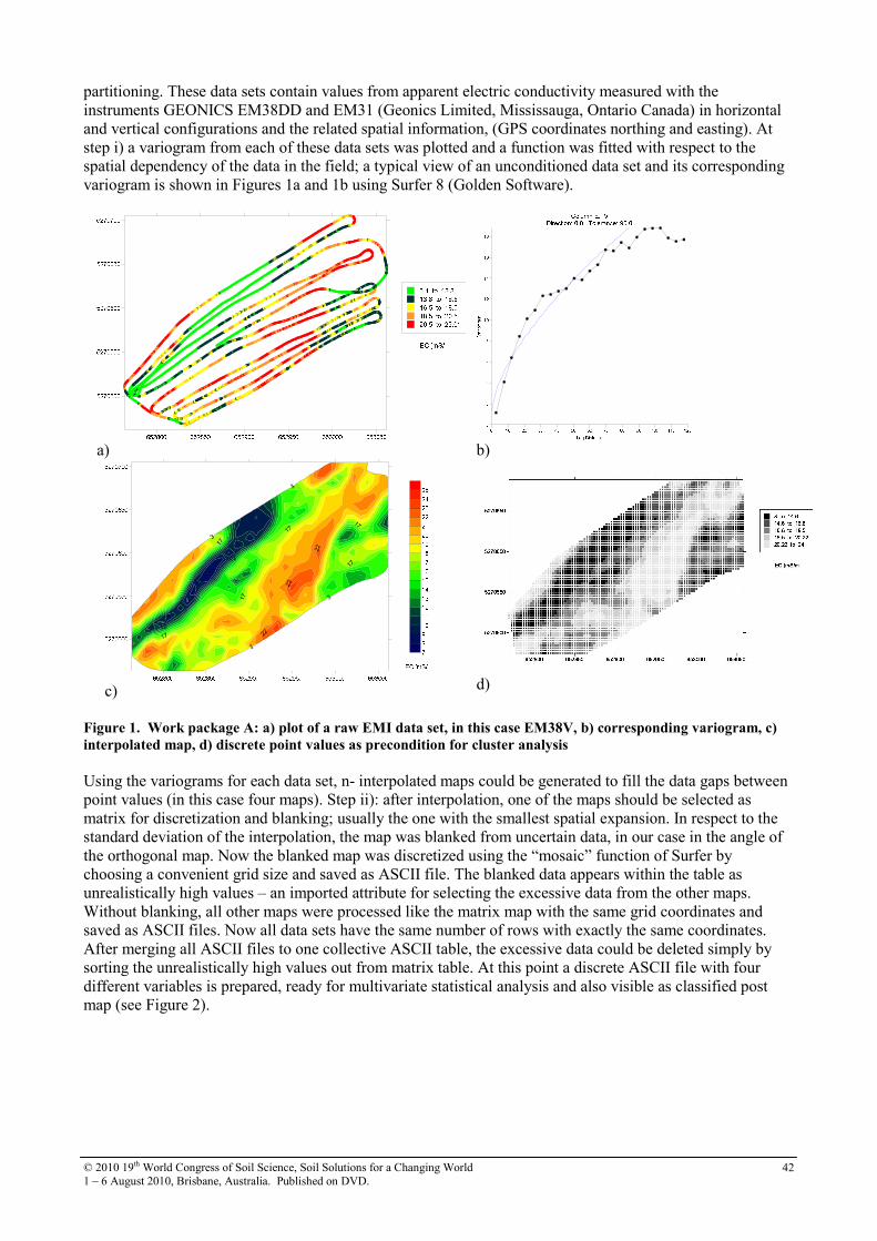
© 2010 19th World Congress of Soil Science, Soil Solutions for a Changing World
1 – 6 August 2010, Brisbane, Australia. Published on DVD. 42
partitioning. These data sets contain values from apparent electric conductivity measured with the
instruments GEONICS EM38DD and EM31 (Geonics Limited, Mississauga, Ontario Canada) in horizontal
and vertical configurations and the related spatial information, (GPS coordinates northing and easting). At
step i) a variogram from each of these data sets was plotted and a function was fitted with respect to the
spatial dependency of the data in the field; a typical view of an unconditioned data set and its corresponding
variogram is shown in Figures 1a and 1b using Surfer 8 (Golden Software).
a)
b)
c)
d)
Figure 1. Work package A: a) plot of a raw EMI data set, in this case EM38V, b) corresponding variogram, c)
interpolated map, d) discrete point values as precondition for cluster analysis
Using the variograms for each data set, n- interpolated maps could be generated to fill the data gaps between
point values (in this case four maps). Step ii): after interpolation, one of the maps should be selected as
matrix for discretization and blanking; usually the one with the smallest spatial expansion. In respect to the
standard deviation of the interpolation, the map was blanked from uncertain data, in our case in the angle of
the orthogonal map. Now the blanked map was discretized using the “mosaic” function of Surfer by
choosing a convenient grid size and saved as ASCII file. The blanked data appears within the table as
unrealistically high values – an imported attribute for selecting the excessive data from the other maps.
Without blanking, all other maps were processed like the matrix map with the same grid coordinates and
saved as ASCII files. Now all data sets have the same number of rows with exactly the same coordinates.
After merging all ASCII files to one collective ASCII table, the excessive data could be deleted simply by
sorting the unrealistically high values out from matrix table. At this point a discrete ASCII file with four
different variables is prepared, ready for multivariate statistical analysis and also visible as classified post
map (see Figure 2).
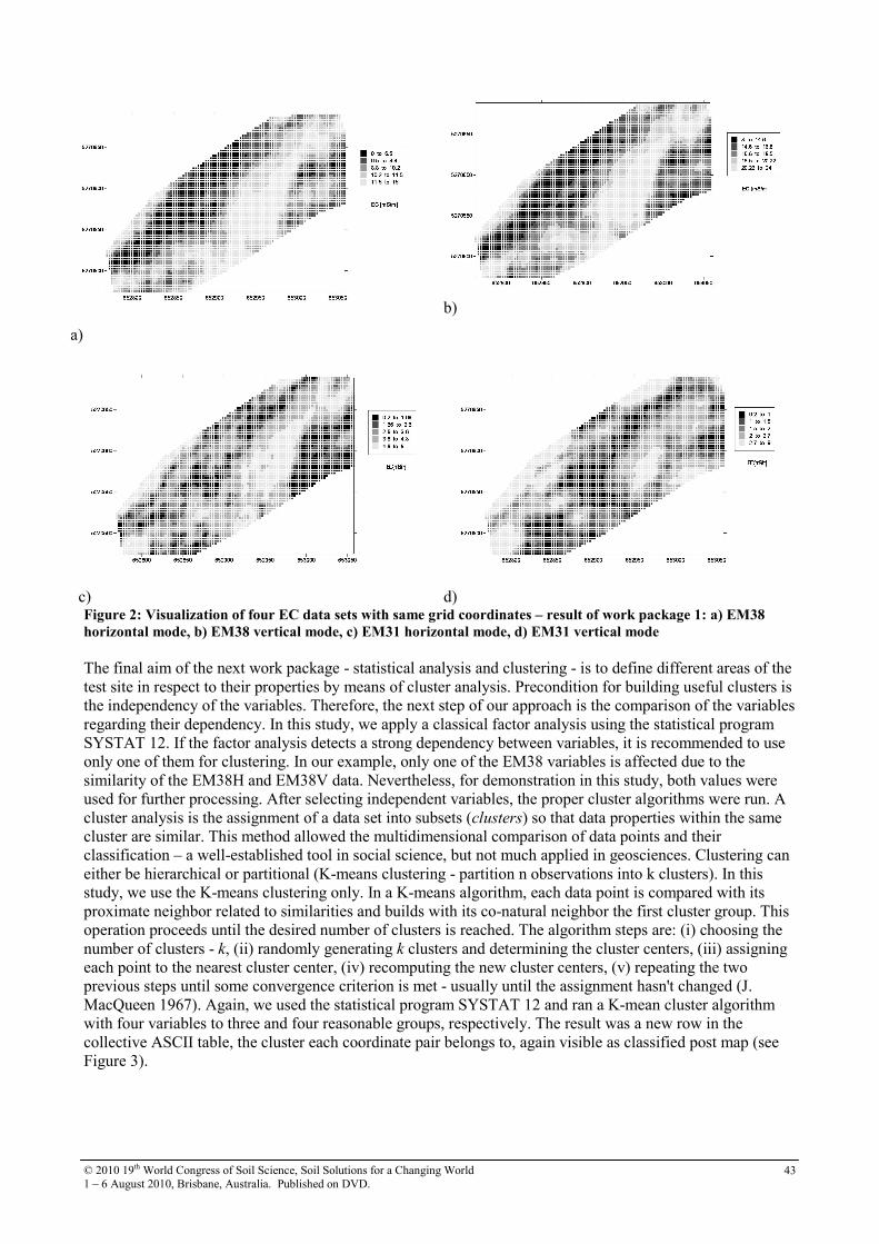
© 2010 19th World Congress of Soil Science, Soil Solutions for a Changing World
1 – 6 August 2010, Brisbane, Australia. Published on DVD. 43
a)
b)
c)
d)
Figure 2: Visualization of four EC data sets with same grid coordinates – result of work package 1: a) EM38
horizontal mode, b) EM38 vertical mode, c) EM31 horizontal mode, d) EM31 vertical mode
The final aim of the next work package - statistical analysis and clustering - is to define different areas of the
test site in respect to their properties by means of cluster analysis. Precondition for building useful clusters is
the independency of the variables. Therefore, the next step of our approach is the comparison of the variables
regarding their dependency. In this study, we apply a classical factor analysis using the statistical program
SYSTAT 12. If the factor analysis detects a strong dependency between variables, it is recommended to use
only one of them for clustering. In our example, only one of the EM38 variables is affected due to the
similarity of the EM38H and EM38V data. Nevertheless, for demonstration in this study, both values were
used for further processing. After selecting independent variables, the proper cluster algorithms were run. A
cluster analysis is the assignment of a data set into subsets (clusters) so that data properties within the same
cluster are similar. This method allowed the multidimensional comparison of data points and their
classification – a well-established tool in social science, but not much applied in geosciences. Clustering can
either be hierarchical or partitional (K-means clustering - partition n observations into k clusters). In this
study, we use the K-means clustering only. In a K-means algorithm, each data point is compared with its
proximate neighbor related to similarities and builds with its co-natural neighbor the first cluster group. This
operation proceeds until the desired number of clusters is reached. The algorithm steps are: (i) choosing the
number of clusters - k, (ii) randomly generating k clusters and determining the cluster centers, (iii) assigning
each point to the nearest cluster center, (iv) recomputing the new cluster centers, (v) repeating the two
previous steps until some convergence criterion is met - usually until the assignment hasn't changed (J.
MacQueen 1967). Again, we used the statistical program SYSTAT 12 and ran a K-mean cluster algorithm
with four variables to three and four reasonable groups, respectively. The result was a new row in the
collective ASCII table, the cluster each coordinate pair belongs to, again visible as classified post map (see
Figure 3).
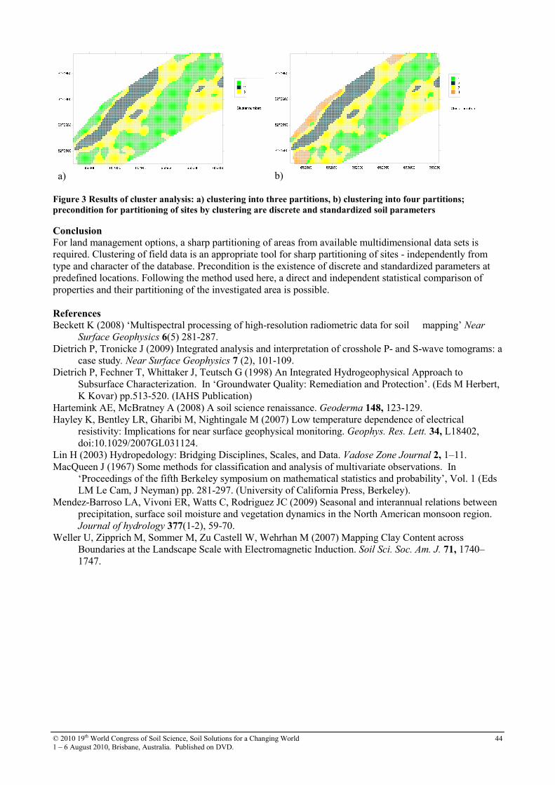
© 2010 19th World Congress of Soil Science, Soil Solutions for a Changing World
1 – 6 August 2010, Brisbane, Australia. Published on DVD. 44
a)
b)
Figure 3 Results of cluster analysis: a) clustering into three partitions, b) clustering into four partitions;
precondition for partitioning of sites by clustering are discrete and standardized soil parameters
Conclusion
For land management options, a sharp partitioning of areas from available multidimensional data sets is
required. Clustering of field data is an appropriate tool for sharp partitioning of sites - independently from
type and character of the database. Precondition is the existence of discrete and standardized parameters at
predefined locations. Following the method used here, a direct and independent statistical comparison of
properties and their partitioning of the investigated area is possible.
References Beckett K (2008) ‘Multispectral processing of high-resolution radiometric data for soil mapping’ Near
Surface Geophysics 6(5) 281-287.
Dietrich P, Tronicke J (2009) Integrated analysis and interpretation of crosshole P- and S-wave tomograms: a
case study. Near Surface Geophysics 7 (2), 101-109.
Dietrich P, Fechner T, Whittaker J, Teutsch G (1998) An Integrated Hydrogeophysical Approach to
Subsurface Characterization. In ‘Groundwater Quality: Remediation and Protection’. (Eds M Herbert,
K Kovar) pp.513-520. (IAHS Publication)
Hartemink AE, McBratney A (2008) A soil science renaissance. Geoderma 148, 123-129.
Hayley K, Bentley LR, Gharibi M, Nightingale M (2007) Low temperature dependence of electrical
resistivity: Implications for near surface geophysical monitoring. Geophys. Res. Lett. 34, L18402,
doi:10.1029/2007GL031124.
Lin H (2003) Hydropedology: Bridging Disciplines, Scales, and Data. Vadose Zone Journal 2, 1–11.
MacQueen J (1967) Some methods for classification and analysis of multivariate observations. In
‘Proceedings of the fifth Berkeley symposium on mathematical statistics and probability’, Vol. 1 (Eds
LM Le Cam, J Neyman) pp. 281-297. (University of California Press, Berkeley).
Mendez-Barroso LA, Vivoni ER, Watts C, Rodriguez JC (2009) Seasonal and interannual relations between
precipitation, surface soil moisture and vegetation dynamics in the North American monsoon region.
Journal of hydrology 377(1-2), 59-70.
Weller U, Zipprich M, Sommer M, Zu Castell W, Wehrhan M (2007) Mapping Clay Content across
Boundaries at the Landscape Scale with Electromagnetic Induction. Soil Sci. Soc. Am. J. 71, 1740–
1747.
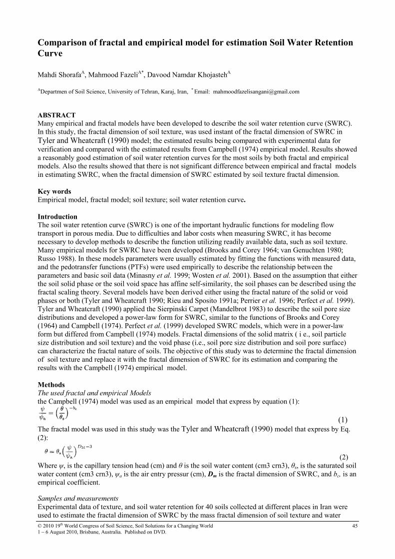
© 2010 19th World Congress of Soil Science, Soil Solutions for a Changing World
1 – 6 August 2010, Brisbane, Australia. Published on DVD. 45
Comparison of fractal and empirical model for estimation Soil Water Retention
Curve
Mahdi Shorafa
A, Mahmood Fazeli
A*, Davood Namdar Khojasteh
A
ADepartmen of Soil Science, University of Tehran, Karaj, Iran, * Email: [email protected]
ABSTRACT
Many empirical and fractal models have been developed to describe the soil water retention curve (SWRC).
In this study, the fractal dimension of soil texture, was used instant of the fractal dimension of SWRC in
Tyler and Wheatcraft (1990) model; the estimated results being compared with experimental data for
verification and compared with the estimated results from Campbell (1974) empirical model. Results showed
a reasonably good estimation of soil water retention curves for the most soils by both fractal and empirical
models. Also the results showed that there is not significant difference between empirical and fractal models
in estimating SWRC, when the fractal dimension of SWRC estimated by soil texture fractal dimension.
Key words Empirical model, fractal model; soil texture; soil water retention curve.
Introduction The soil water retention curve (SWRC) is one of the important hydraulic functions for modeling flow
transport in porous media. Due to difficulties and labor costs when measuring SWRC, it has become
necessary to develop methods to describe the function utilizing readily available data, such as soil texture.
Many empirical models for SWRC have been developed (Brooks and Corey 1964; van Genuchten 1980;
Russo 1988). In these models parameters were usually estimated by fitting the functions with measured data,
and the pedotransfer functions (PTFs) were used empirically to describe the relationship between the
parameters and basic soil data (Minasny et al. 1999; Wosten et al. 2001). Based on the assumption that either
the soil solid phase or the soil void space has affine self-similarity, the soil phases can be described using the
fractal scaling theory. Several models have been derived either using the fractal nature of the solid or void
phases or both (Tyler and Wheatcraft 1990; Rieu and Sposito 1991a; Perrier et al. 1996; Perfect et al. 1999).
Tyler and Wheatcraft (1990) applied the Sierpinski Carpet (Mandelbrot 1983) to describe the soil pore size
distributions and developed a power-law form for SWRC, similar to the functions of Brooks and Corey
(1964) and Campbell (1974). Perfect et al. (1999) developed SWRC models, which were in a power-law
form but differed from Campbell (1974) models. Fractal dimensions of the solid matrix ( i e., soil particle
size distribution and soil texture) and the void phase (i.e., soil pore size distribution and soil pore surface)
can characterize the fractal nature of soils. The objective of this study was to determine the fractal dimension
of soil texture and replace it with the fractal dimension of SWRC for its estimation and comparing the
results with the Campbell (1974) empirical model.
Methods The used fractal and empirical Models
the Campbell (1974) model was used as an empirical model that express by equation (1):
(1)
The fractal model was used in this study was the Tyler and Wheatcraft (1990) model that express by Eq.
(2):
(2)
Where ψ, is the capillary tension head (cm) and θ is the soil water content (cm3 crn3), θs, is the saturated soil
water content (cm3 crn3), ψa is the air entry pressur (cm), Dm is the fractal dimension of SWRC, and bc, is an
empirical coefficient.
Samples and measurements
Experimental data of texture, and soil water retention for 40 soils collected at different places in Iran were
used to estimate the fractal dimension of SWRC by the mass fractal dimension of soil texture and water
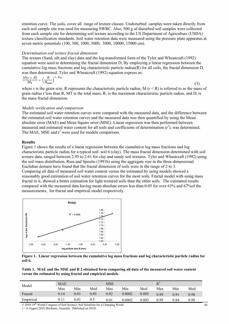
© 2010 19th World Congress of Soil Science, Soil Solutions for a Changing World
1 – 6 August 2010, Brisbane, Australia. Published on DVD. 46
retention curve. The soils, cover all range of texture classes. Undisturbed samples were taken directly from
each soil sample site was used for measuring SWRC. Also, 500 g of disturbed soil samples were collected
from each sample site for determining soil texture according to the US Department of Agriculture (USDA)
texture classification standards. Soil water retention data were measured using the pressure plate apparatus at
seven metric potentials (100, 300, 1000, 3000, 5000, 10000, 15000 cm).
Determination soil texture fractal dimension
The texture (Sand, silt and clay) data and the log-transformed form of the Tyler and Wheatcraft (1992)
equation were used to determining the fractal dimension D; By employing a linear regression between the
cumulative log mass fractions and log characteristic particle radius(R) for all soils, the fractal dimension D,
was then determined. Tyler and Wheatcraft (1992) equation express as:
(3)
where r is the grain size, R represents the characteristic particle radius, M (r < R) is referred to as the mass of
grain radius r less than R, MT is the total mass, R, is the maximum characteristic particle radius, and D, is
the mass fractal dimension.
Models verification and comparison
The estimated soil water retention curves were compared with the measured data, and the difference between
the estimated soil water retention curves and the measured data was then quantified by using the Mean
absolute error (MAE) and Mean Square error (MSE). Linear regression was then performed between
measured and estimated water content for all soils and coefficients of determination (r2), was determined.
The MAE, MSE and r2 were used for models comparison.
Results Figure 1 shows the results of a linear regression between the cumulative log mass fractions and log
characteristic particle radius for a typical soil: soil 6 (clay). The mass fractal dimension determined with soil
texture data, ranged between 2.95 to 2.61 for clay and sandy soil textures. Tyler and Wheatcraft (1992) using
the soil mass distribution, Rieu and Sposito (1991b) using the aggregate size in the three-dimensional
Euclidian domain have found that the fractal dimension of soils were in the range of 2 to 3.
Comparing all data of measured soil water content versus the estimated by using models showed a
reasonably good estimation of soil water retention curves for the most soils. Fractal model with using mass
fractal in it, showed a better estimation for light textured soils than the other soils. The estimated results
compared with the measured data having mean absolute errors less than 0.05 for over 63% and 67%of the
measurements, for fractal and empirical model respectively.
6(clay)
R2 = 0.9958
1.60
1.62
1.64
1.66
1.68
1.70
1.72
1.74
1.76
1.78
1.80
-3.00 -2.50 -2.00 -1.50 -1.00 -0.50 0.00 0.50
log particle size,R,(mm)
log m
ass fraction(r<R)
Figure 1. Linear regression between the cumulative log mass fractions and log characteristic particle radius for
soil 6.
Table 1. MAE and the MSE and R 2 obtained form comparing all data of the measured soil water content
versus the estimated by using fractal and empirical models.
MAE MSE R2
Model Max Min Mod Max Min Mod Max Min Mod
Fractal 0.14 0.01 0.05 0.02 0.0002 0.005 0.99 0.91 0.98
Empirical 0.11 0.01 0.5 0.01 0.0002 0.003 0.99 0.84 0.98
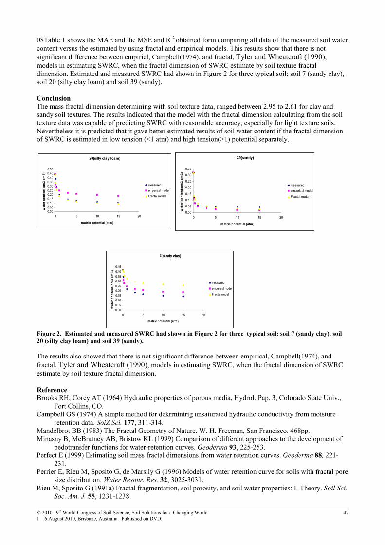
© 2010 19th World Congress of Soil Science, Soil Solutions for a Changing World
1 – 6 August 2010, Brisbane, Australia. Published on DVD. 47
08Table 1 shows the MAE and the MSE and R 2 obtained form comparing all data of the measured soil water
content versus the estimated by using fractal and empirical models. This results show that there is not
significant difference between empiricl, Campbell(1974), and fractal, Tyler and Wheatcraft (1990), models in estimating SWRC, when the fractal dimension of SWRC estimate by soil texture fractal
dimension. Estimated and measured SWRC had shown in Figure 2 for three typical soil: soil 7 (sandy clay),
soil 20 (silty clay loam) and soil 39 (sandy).
Conclusion The mass fractal dimension determining with soil texture data, ranged between 2.95 to 2.61 for clay and
sandy soil textures. The results indicated that the model with the fractal dimension calculating from the soil
texture data was capable of predicting SWRC with reasonable accuracy, especially for light texture soils.
Nevertheless it is predicted that it gave better estimated results of soil water content if the fractal dimension
of SWRC is estimated in low tension (<1 atm) and high tension(>1) potential separately.
20(silty clay loam)
0.00
0.05
0.10
0.15
0.20
0.25
0.30
0.35
0.40
0.45
0.50
0 5 10 15 20
matric potential (atm)
water content(cm3 cm3)
measured
emperical model
Fractal model
39(sandy)
0.00
0.05
0.10
0.15
0.20
0.25
0.30
0.35
0 5 10 15 20
matric potential (atm)
water content(cm3 cm3)
measured
emperical model
Fractal model
7(sandy clay)
0.00
0.05
0.10
0.15
0.20
0.25
0.30
0.35
0.40
0.45
0 5 10 15 20
matric potential (atm)
water content(cm3 cm3)
measured
emperical model
Fractal model
Figure 2. Estimated and measured SWRC had shown in Figure 2 for three typical soil: soil 7 (sandy clay), soil
20 (silty clay loam) and soil 39 (sandy).
The results also showed that there is not significant difference between empirical, Campbell(1974), and
fractal, Tyler and Wheatcraft (1990), models in estimating SWRC, when the fractal dimension of SWRC
estimate by soil texture fractal dimension.
Reference Brooks RH, Corey AT (1964) Hydraulic properties of porous media, Hydrol. Pap. 3, Colorado State Univ.,
Fort Collins, CO.
Campbell GS (1974) A simple method for dekrrninirig unsaturated hydraulic conductivity from moisture
retention data. SoiZ Sci. 177, 311-314.
Mandelbrot BB (1983) The Fractal Geometry of Nature. W. H. Freeman, San Francisco. 468pp.
Minasny B, McBratney AB, Bristow KL (1999) Comparison of different approaches to the development of
pedotransfer functions for water-retention curves. Geoderma 93, 225-253.
Perfect E (1999) Estimating soil mass fractal dimensions from water retention curves. Geoderma 88, 221-
231.
Perrier E, Rieu M, Sposito G, de Marsily G (1996) Models of water retention curve for soils with fractal pore
size distribution. Water Resour. Res. 32, 3025-3031.
Rieu M, Sposito G (1991a) Fractal fragmentation, soil porosity, and soil water properties: I. Theory. Soil Sci.
Soc. Am. J. 55, 1231-1238.

© 2010 19th World Congress of Soil Science, Soil Solutions for a Changing World
1 – 6 August 2010, Brisbane, Australia. Published on DVD. 48
Rieu M, Sposito G (1991b) Fractal fragmentation, soil porosity and soil water properties: 11. Applications.
Soil Sci.
Russo D (1988) Determining soil hydraulic properties by parameter estimation: On the selection of a model
for the hydraulic properties. Water Resour. Res. 24, 453-459.
Tyler SW, Wheatcraft SW (1990) Fractal processes in soil water retention. Water Resour. Res. 26, 1047-
1054.
Tyler SW, Wheatcraft SW (1992) Fractal scaling of soil particle size distributions: Analysis and limitations.
Soil
van Genuchten MTh (1980) A closed-form equation for predicting the hydraulic conductivity of unsaturated
soils. Soil
Wosten JHM, van Genuchten MTh (1988) Using texture and other soil properties to predict the unsaturated
soil hydraulic functions. Soil Sci. Soc Am. J. 52, 1762-1 770.
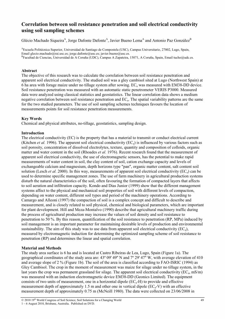
© 2010 19th World Congress of Soil Science, Soil Solutions for a Changing World
1 – 6 August 2010, Brisbane, Australia. Published on DVD. 49
Correlation between soil resistance penetration and soil electrical conductivity
using soil sampling schemes
Glécio Machado SiqueiraA, Jorge Dafonte Dafonte
A, Javier Bueno Lema
A and Antonio Paz González
B
AEscuela Politécnica Superior, Universidad de Santiago de Compostela (USC), Campus Universitario, 27002, Lugo, Spain,
Email [email protected]; [email protected]; [email protected]. BFacultad de Ciencias, Universidad de A Coruña (UDC), Campus A Zapateira, 15071, A Coruña, Spain, Email [email protected].
Abstract The objective of this research was to calculate the correlation between soil resistance penetration and
apparent soil electrical conductivity. The studied soil was a gley cambisol sited at Lugo (Northwest Spain) at
6 ha area with forage maize under no tillage system after sowing. ECa was measured with EM38-DD device.
Soil resistance penetration was measured with an automatic static penetrometer VERIS P3000. Measured
data were analyzed using classical statistics and geostatistics. The linear correlation data shows a medium
negative correlation between soil resistance penetration and ECa. The spatial variability patterns are the same
for the two studied parameters. The use of soil sampling schemes techniques favours the location of
measurements points for soil resistance penetration measurements.
Key Words Chemical and physical attributes, no-tillage, geostatistics, sampling design.
Introduction The electrical conductivity (EC) is the property that has a material to transmit or conduct electrical current
(Kitchen et al. 1996). The apparent soil electrical conductivity (ECa) is influenced by various factors such as
soil porosity, concentration of dissolved electrolytes, texture, quantity and composition of colloids, organic
matter and water content in the soil (Rhoades et al. 1976). Recent research found that the measurement of
apparent soil electrical conductivity, the use of electromagnetic sensors, has the potential to make rapid
measurements of water content in soil, the clay content of soil, cation exchange capacity and levels of
exchangeable calcium and magnesium, depth horizons type "pan", organic matter content, salt content soil
solution (Lesch et al. 2000). In this way, measurements of apparent soil electrical conductivity (ECa) can be
used to determine specific management zones. The use of farm machinery in agricultural production systems
disturb the natural characteristics of the soil, often favouring the formation of compacted layers that affects
to soil aeration and infiltration capacity. Kondo and Dias Junior (1999) show that the different management
systems affect to the physical and mechanical soil properties of soil with different levels of compaction,
depending on water content, different soil types and period of the machinery operations. According to
Camargo and Alleoni (1997) the compaction of soil is a complex concept and difficult to describe and
measurement, and is closely related to soil physical, chemical and biological parameters, which are important
for plant development. Hill and Meza-Montalvo (1990) describe that agricultural machinery traffic during
the process of agricultural production may increase the values of soil density and soil resistance to
penetration to 50 %. By this reason, quantification of the soil resistance to penetration (RP, MPa) induced by
soil management is an important parameter for maintaining desirable levels of production and environmental
sustainability. The aim of this study was to use data from apparent soil electrical conductivity (ECa),
measured by electromagnetic induction for determining the optimized sampling scheme of soil resistance to
penetration (RP) and determines the linear and spatial correlation.
Material and Methods The study area surface is 6 ha and is located at Castro Ribeiras de Lea, Lugo, Spain (Figure 1a). The
geographical coordinates of the study area are: 43º 09' 49'' N and 7º 29' 47'' W, with average elevation of 410
and average slope of 2 % (Figure 1b). The soil of the area is classified according to FAO-ISRIC (1994) as
Gley Cambisol. The crop in the moment of measurement was maize for silage under no tillage system, in the
last years the crop was permanent grassland for silage. The apparent soil electrical conductivity (ECa, mS/m)
was measured with an induction electromagnetic device EM38-DD (Geonics Limited). The equipment
consists of two units of measurement, one in a horizontal dipole (ECa-H) to provide and effective
measurement depth of approximately 1.5 m and other one in vertical dipole (ECa-V) with an effective
measurement depth of approximately 0.75 m (McNeill 1980). The data were collected on 23/06/2008 in
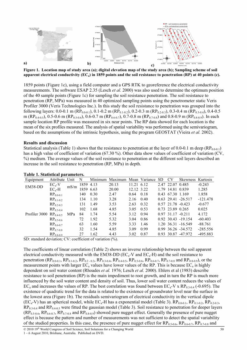
© 2010 19th World Congress of Soil Science, Soil Solutions for a Changing World
1 – 6 August 2010, Brisbane, Australia. Published on DVD. 50
a)
Castro de Ribeiras de
Lea (Lugo, Spain)
b) 622550 622600 622650 622700 622750 622800
Distance X (m)
4779650
4779700
4779750
4779800
4779850
4779900
Distance Y (m)
406
409
412
c) 622500 622550 622600 622650 622700 622750 622800
Distance X (m)
4779650
4779700
4779750
4779800
4779850
4779900
Dis
tanceY
(m
)
RP - soil resistence penetratión
ECa- soil electrical conductivity
Figure 1. Location map of study area (a); digital elevation map of the study area (b); Sampling scheme of soil
apparent electrical conductivity (ECa) in 1859 points and the soil resistance to penetration (RP) at 40 points (c).
1859 points (Figure 1c), using a field computer and a GPS RTK to georeference the electrical conductivity
measurements. The software ESAP 2.35 (Lesch et al. 2000) was also used to determine the optimum position
of the 40 sample points (Figure 1c) for sampling the soil resistance penetration. The soil resistance to
penetration (RP, MPa) was measured in 40 optimized sampling points using the penetrometer static Veris
Profiler 3000 (Veris Technologies Inc.). In this study the soil resistance to penetration was grouped into the
following layers: 0.0-0.1 m (RP0.0-0.1), 0.1-0.2 m (RP0.1-0.2), 0.2-0.3 m (RP0.2-0.3), 0.3-0.4 m (RP0.3-0.4), 0.4-0.5
m (RP0.4-0.5), 0.5-0.6 m (RP0.5-0.6), 0.6-0.7 m (RP0.6-0.7), 0.7-0.8 m (RP0.7-0.8) and 0.8-0.9 m (RP0.8-0.9). In each
sample location RP profile was measured in six near points. The RP data showed for each location is the
mean of the six profiles measured. The analysis of spatial variability was performed using the semivariogram,
based on the assumptions of the intrinsic hypothesis, using the program GEOSTAT (Vieira et al. 2002).
Results and discussion Statistical analysis (Table 1) shows that the resistance to penetration at the layer of 0.0-0.1 m deep (RP0.0-0.1)
has a high value of coefficient of variation (67.30 %). Other data show values of coefficient of variation (CV,
%) medium. The average values of the soil resistance to penetration at the different soil layers described an
increase in the soil resistance to penetration (RP, MPa) in depth.
Table 1. Statistical parameters. Equipment Attribute Unit N Minimum Maximum Mean Variance SD CV Skewness Kurtosis
ECa-V 1859 4.13 20.13 11.21 6.12 2.47 22.07 0.485 -0.243 EM38-DD
ECa-H mS/m
1859 6.63 20.00 12.12 3.22 1.79 14.81 0.839 1.285
RP0.0-0.1 140 0.30 2.47 0.64 0.18 0.43 67.30 1.169 1.858
RP0.1-0.2 134 1.10 3.28 2.16 0.40 0.63 29.41 -26.517 -121.478
RP0.2-0.3 131 1.49 3.53 2.63 0.32 0.57 21.78 -0.423 -0.677
RP0.3-0.4 102 1.68 4.85 3.05 0.53 0.73 23.89 0.265 0.025
RP0.4-0.5 84 1.74 5.54 3.12 0.94 0.97 31.17 -0.211 4.172
RP0.5-0.6 72 1.92 5.32 3.04 0.86 0.92 30.43 -19.154 -60.403
RP0.6-0.7 63 1.60 5.59 3.33 1.46 1.20 36.31 -16.549 -88.761
RP0.7-0.8 32 1.54 4.85 3.09 0.99 0.99 36.26 -34.572 -285.556
Profiler 3000
RP0.8-0.9
MPa
27 1.62 4.43 3.02 0.87 0.93 30.87 -47.972 -495.883
SD: standard deviation; CV: coefficient of variation (%).
The coefficients of linear correlation (Table 2) shows an inverse relationship between the soil apparent
electrical conductivity measured with the EM38-DD (ECa-V and ECa-H) and the soil resistance to
penetration (RP0.0-0.1, RP0.1-0.2, RP0.2 - 0.3, RP0.3-0.4, RP0.4-0.5, RP0.5-0.6, RP0.6-0.7, RP0.7-0.8 and RP0.8-0.9), or the
measurement points with larger ECa values have lower values of the RP. This is because ECa is highly
dependent on soil water content (Rhoades et al. 1976; Lesch et al. 2000). Ehlers et al (1983) describe
resistance to soil penetration (RP) is the main impediment to root growth, and in turn the RP is much more
influenced by the soil water content and density of soil. Thus, lower soil water content reduces the values of
ECa and increases the values of RP. The best correlation was found between ECa-V x RP0.3-0.4 (-0.695). The
existence of quadratic trend for the data is related to the existence of groundwater level near the surface in
the lowest area (Figure 1b). The residuals semivariogram of electrical conductivity in the vertical dipole
(ECa-V) has an spherical model, while ECa-H has a exponential model (Table 3). RP0.0-0.1, RP0.1-0.2, RP0.2-0.3,
RP0.3-0.4 and RP0.4-0.5 were fitted the gaussian model (Table 3). Soil resistance to penetration for deeper layers
(RP0.5-0.6, RP0.6-0.7, RP0.7-0.8 and RP0.8-0.9) showed pure nugget effect. Generally the presence of pure nugget
effect is because the pattern and number of measurements was not sufficient to detect the spatial variability
of the studied properties. In this case, the presence of pure nugget effect for RP0.5-0.6, RP0.6-0.7, RP0.7-0.8 and
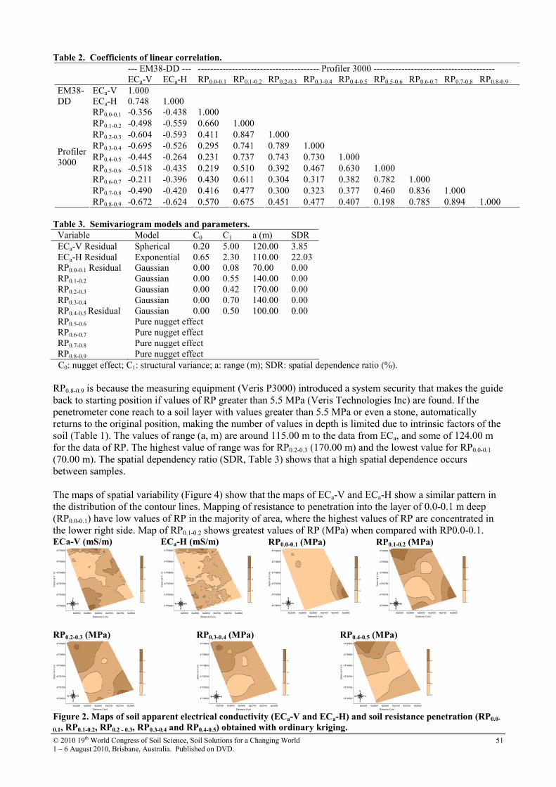
© 2010 19th World Congress of Soil Science, Soil Solutions for a Changing World
1 – 6 August 2010, Brisbane, Australia. Published on DVD. 51
Table 2. Coefficients of linear correlation.
--- EM38-DD --- --------------------------------------- Profiler 3000 ---------------------------------------
ECa-V ECa-H RP0.0-0.1 RP0.1-0.2 RP0.2-0.3 RP0.3-0.4 RP0.4-0.5 RP0.5-0.6 RP0.6-0.7 RP0.7-0.8 RP0.8-0.9
ECa-V 1.000 EM38-
DD ECa-H 0.748 1.000
RP0.0-0.1 -0.356 -0.438 1.000
RP0.1-0.2 -0.498 -0.559 0.660 1.000
RP0.2-0.3 -0.604 -0.593 0.411 0.847 1.000
RP0.3-0.4 -0.695 -0.526 0.295 0.741 0.789 1.000
RP0.4-0.5 -0.445 -0.264 0.231 0.737 0.743 0.730 1.000
RP0.5-0.6 -0.518 -0.435 0.219 0.510 0.392 0.467 0.630 1.000
RP0.6-0.7 -0.211 -0.396 0.430 0.611 0.304 0.317 0.382 0.782 1.000
RP0.7-0.8 -0.490 -0.420 0.416 0.477 0.300 0.323 0.377 0.460 0.836 1.000
Profiler
3000
RP0.8-0.9 -0.672 -0.624 0.570 0.675 0.451 0.477 0.407 0.198 0.785 0.894 1.000
Table 3. Semivariogram models and parameters.
Variable Model C0 C1 a (m) SDR
ECa-V Residual Spherical 0.20 5.00 120.00 3.85
ECa-H Residual Exponential 0.65 2.30 110.00 22.03
RP0.0-0.1 Residual Gaussian 0.00 0.08 70.00 0.00
RP0.1-0.2 Gaussian 0.00 0.55 140.00 0.00
RP0.2-0.3 Gaussian 0.00 0.42 170.00 0.00
RP0.3-0.4 Gaussian 0.00 0.70 140.00 0.00
RP0.4-0.5 Residual Gaussian 0.00 0.50 100.00 0.00
RP0.5-0.6 Pure nugget effect
RP0.6-0.7 Pure nugget effect
RP0.7-0.8 Pure nugget effect
RP0.8-0.9 Pure nugget effect
C0: nugget effect; C1: structural variance; a: range (m); SDR: spatial dependence ratio (%).
RP0.8-0.9 is because the measuring equipment (Veris P3000) introduced a system security that makes the guide
back to starting position if values of RP greater than 5.5 MPa (Veris Technologies Inc) are found. If the
penetrometer cone reach to a soil layer with values greater than 5.5 MPa or even a stone, automatically
returns to the original position, making the number of values in depth is limited due to intrinsic factors of the
soil (Table 1). The values of range (a, m) are around 115.00 m to the data from ECa, and some of 124.00 m
for the data of RP. The highest value of range was for RP0.2-0.3 (170.00 m) and the lowest value for RP0.0-0.1
(70.00 m). The spatial dependency ratio (SDR, Table 3) shows that a high spatial dependence occurs
between samples.
The maps of spatial variability (Figure 4) show that the maps of ECa-V and ECa-H show a similar pattern in
the distribution of the contour lines. Mapping of resistance to penetration into the layer of 0.0-0.1 m deep
(RP0.0-0.1) have low values of RP in the majority of area, where the highest values of RP are concentrated in
the lower right side. Map of RP0.1-0.2 shows greatest values of RP (MPa) when compared with RP0.0-0.1. ECa-V (mS/m)
622550 622600 622650 622700 622750 622800
Distancia X (m)
4779650
4779700
4779750
4779800
4779850
4779900
Dis
tancia
Y (
m)
6
10
14
18
ECa-H (mS/m)
622550 622600 622650 622700 622750 622800
Distancia X (m)
4779650
4779700
4779750
4779800
4779850
4779900
Dis
tancia
Y (
m)
8
12
16
20
RP0.0-0.1 (MPa)
622550 622600 622650 622700 622750 622800
Distancia X (m)
4779650
4779700
4779750
4779800
4779850
4779900
Dis
tan
cia
Y (
m)
0.3
0.9
1.5
2.1
RP0.1-0.2 (MPa)
622550 622600 622650 622700 622750 622800
Distancia X (m)
4779650
4779700
4779750
4779800
4779850
4779900
Dis
tan
cia
Y (
m)
1.1
1.7
2.3
2.9
RP0.2-0.3 (MPa)
622550 622600 622650 622700 622750 622800
Distancia X (m)
4779650
4779700
4779750
4779800
4779850
4779900
Dis
tan
cia
Y (
m)
1.5
2.1
2.7
3.3
RP0.3-0.4 (MPa)
622550 622600 622650 622700 622750 622800
Distancia X (m)
4779650
4779700
4779750
4779800
4779850
4779900
Dis
tan
cia
Y (
m)
1.6
2.5
3.4
4.3
RP0.4-0.5 (MPa)
622550 622600 622650 622700 622750 622800
Distancia X (m)
4779650
4779700
4779750
4779800
4779850
4779900
Dis
tan
cia
Y (
m)
1.6
2.6
3.6
4.6
Figure 2. Maps of soil apparent electrical conductivity (ECa-V and ECa-H) and soil resistance penetration (RP0.0-
0.1, RP0.1-0.2, RP0.2 - 0.3, RP0.3-0.4 and RP0.4-0.5) obtained with ordinary kriging.

© 2010 19th World Congress of Soil Science, Soil Solutions for a Changing World
1 – 6 August 2010, Brisbane, Australia. Published on DVD. 52
The maps of soil resistance to penetration (RP0.2-0.3, RP0.3-0.4 and RP0.4-0.5) show similar pattern to RP0.1-0.2
map. The presence of the highest values of RP (MPa) in the upper part of the area coincides with the maps of
ECa-V and ECa-H that have lower values of ECa in this area, corroborating the data of Table 2 that shows an
inverse relationship between electrical conductivity and the soil resistance to penetration. In this way, the use
of electrical conductivity data for optimizing the sampling of the soil resistance to penetration proves its
efficiency mainly because the two variables are correlated with soil water content.
Conclusions The data of EC and RP showed low values of coefficient of variation (CV, %), except for the soil resistance
to penetration into the layer of 0.0-0.1 m depth that has a high value of CV (60.30 %). The gaussian model
was fitted to the data of soil resistance penetration (RP0.0-0.1, RP0.1-0.2, RP0.2-0.3, RP0.3-0.4 and RP0.4-0.5). The
presence of pure nugget effect for data for soil resistance penetration in depth (RP0.5-0.6, RP0.6-0.7, RP0.7-0.8 and
RP0.8-0.9) is caused by to the limited number of data in these layers once in this layer the values were often
higher than the measurement value limit of the equipment (5.5 MPa). Data of apparent soil electrical
conductivity (ECa) was used to determine the optimized sampling scheme of the soil resistance penetration
(RP), this methodology has proved to be efficient and capable for representing the spatial variability pattern
of soil resistance penetration (RP). The maps of spatial variability shows the inverse correlation between the
data of ECa and RP, the areas with higher values of ECa-v and ECa-H have smaller values of RP once both
properties are related to the soil water content.
Acknowledgements The authors are grateful to the Ministerio de Asuntos Exteriores y de Cooperación (MAEC-AECID) from
Spain for the granting of scholarships for PhD studies. This work has been funded by Ministerio de
Educación y Ciencia, within the framework of research project CGL2005-08219-C02-022, co-funded by
Xunta de Galicia, within the framework of research project PGIDIT06PXIC291062PN and by the European
Regional Development Fund (ERDF).
Referenecs Camargo OA, Alleoni LRF (1997) ‘Compactação do solo e o desenvolvimento das plantas’. (Piracicaba).
Ehlers WE, Köpke F, Hesse F, Böhm W (1983) Penetration resistance and root growth of oats in tilled and
untilled loess soil. Soil & Tillage Research 3, 261-275.
Hill RL, Meza-Montalvo M (1990) Long-term wheel traffic effects on soil physical properties under
different tillage systems. Soil Science Society of America Journal 54, 865-870.
Kitchen NR, Sudduth KA, Drummond ST (1996) Mapping of sand deposition from 1993 midwest floods
with electromagnetic induction measurements. Journal of Soil and Water Conservation 51, 336-340.
Kondo MK, Dias Júnior MS (1999) Compressibilidade de três Latossolos em função da umidade e uso.
Revista Brasileira de Ciência do Solo 23, 211-218.
Lesch S.M, Rhoades JD, Corwin DL (2000) ‘The ESAP Version 2.01r User Manual and Tutorial Guide’.
Research Report v.146. (Salinity Laboratory: Riverside, CA) (currently under review).
Rhoades JD, Raats PAC, Prather RJ (1976) Effects of liquid-phase electrical conductivity, water content and
surface conductivity on bulk soil electrical conductivity. Soil Science Society of America Journal 40, 651-
655.
Schueller JKA (2000) Agricultura de precisão: visão externa. O estado-da-arte da agricultura de Precisão nos
Estados Unidos. In ‘Estudo da arte da agricultura de precisão no Brasil’. Vol.1, (Ed LA Balastreire). pp.
8-16.
© 2010 19th World Congress of Soil Science, Soil Solutions for a Changing World
1 – 6 August 2010, Brisbane, Australia. Published on DVD. 53
Creating soil degradation maps using gamma-ray signatures
Petra ErbeA, Ulrich Schuler
B, Suwimon Wicharuck
A, Wanida Rangubpit
A, Karl Stahr
C & Ludger Herrmann
C
AThe Uplands Program, Hohenheim Office, Faculty of Agriculture, Chiang Mai University, Chiang Mai 50200, Thailand BFederal Institute for Geosciences and Natural Resources (BGR), B2.2 Spatial Information Soil and Water,
Stilleweg 2, 30655 Hanover, Germany CUniversity of Hohenheim, Institute of Soil Science and Land Evaluation (310), 70593 Stuttgart, Germany
Abstract The uplands of northwestern Thailand are highly susceptible to soil erosion. The high degree of soil
degradation originates mainly from unsustainable farming practices on steep terrain. The situation could be
improved by sustainable land use planning. Therefore information is needed about the location of erosion-
prone areas and the state of soil degradation. Our study aims to provide decision makers with maps
containing these informations. As the determination of actual soil erosion rates can be time consuming, we
tested if radio signatures (K, eTh) can be used as proxies. Therefore, we compared the data of topsoil
thickness and erosion measurements by Gerlach troughs with the gamma-ray signatures of these sites in an
upland rice field in Mae Hong Son province. The results show a significant correlation between the erosion
measurements and the K/eTh ratio. As next step an interpolated erosion map will be created using the data
collected from the Gerlach troughs. This map will be overlain with the interpolated radiometry map in order
to calculate the goodness of their fitting. If the fitting is significant, such gamma-ray interpolation maps can
be used to pinpoint erosion hot spots on field scale and give information about the actual state of soil
degradation.
Key Words Erosion hazard zones, sloping land, rainfed rice field, northern Thailand, radiometry
Introduction The livelihoods of farmers in northwestern Thailand depend on the quality of the soils on which they
cultivate their crops. Unfortunately the erosion on these already due to their steepness (mostly >25 degrees)
highly endangered soils is further expedited by unsustainable land use practices, like shortening of the
traditional fallow period or the intensive cultivation of upland rice and maize (Schuler 2008). These practices
result in strongly eroded soils, leaving in certain areas less than 10 cm of topsoil thickness. The further
deterioration of the sloped farmland could be avoided by sustainable land use planning. Our study aims to
provide decision makers with maps indicating the location of high risk erosion spots within the fields and the
state of actual soil degradation. These soil degradation maps would enable them to plan and implement
adapted anti-erosion measures like vetiver grass strips (Mattiga and Nareuban 2005) or convince farmers to
change the land use for such fields altogether.
For the production of such soil degradation maps detailed information about the specific erosion rates of
each field would be needed. As this is a time consuming process, we tested if radio signatures, which are
more rapidly measured, can be used as proxies for soil erosion. The basis for this approach is the fact that
illuviation type soils are dominant in Northern Thailand and that in these soils the Bt-horizon contains a
higher concentration of K-rich clay minerals than the overlying eluviated topsoil. Hence, when the topsoil is
eroded, the K-rich Bt-horizon is closer to the surface enhancing the K-radio signature (Wilford 1995; Tyler
2008; Schuler et al. 2009).
Material & Methods For this study we selected an obviously highly eroded upland rice field near the village Bor Krai in Phang
Ma Pha District, Mae Hong Son Province, northwestern Thailand. The soil of the rice field is classified
according to WRB 2006 (IUSS Working Group 2006) as Alisol. The parent material is claystone (Schuler
2008). On this field 21 Gerlach troughs (=GT, in 6 rows, each containing 2-4 GTs, distributed over the slope
in a W-shape) are installed, which are used to measure the soil loss and deposition along the slope taking
each Gerlach trough’s catchment area and the discharge of the respective upslope row into account. At all
GT locations the radio signatures of potassium (K) and thorium equivalent (eTh) were measured once in the
dry season using a GRM-260 handheld radiometric device (Gf Instruments, s.r.o. Geophysical Equipment
and Services, Czech Republic). Additionally inclination and topsoil thickness were measured at the Gerlach
trough positions as well as in between once at the end of the rainy season. In order to test radio signatures as
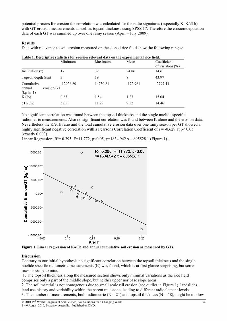
© 2010 19th World Congress of Soil Science, Soil Solutions for a Changing World
1 – 6 August 2010, Brisbane, Australia. Published on DVD. 54
potential proxies for erosion the correlation was calculated for the radio signatures (especially K, K/eTh)
with GT-erosion measurements as well as topsoil thickness using SPSS 17. Therefore the erosion/deposition
data of each GT was summed up over one rainy season (April – July 2009).
Results Data with relevance to soil erosion measured on the sloped rice field show the following ranges:
Table 1. Descriptive statistics for erosion relevant data on the experimental rice field.
Minimum Maximum Mean Coefficient
of variation (%)
Inclination (°) 17 32 24.86 14.6
Topsoil depth (cm) 3 19 8 43.97
Cumulative
annual erosion/GT
(kg ha-1)
-12926.80 14730.81 -172.961 -2797.43
K (%) 0.83 1.54 1.23 15.04
eTh (%) 5.05 11.29 9.52 14.46
No significant correlation was found between the topsoil thickness and the single nuclide specific
radiometric measurements. Also no significant correlation was found between K alone and the erosion data.
Nevertheless the K/eTh ratio and the total cumulative erosion data over one rainy season per GT showed a
highly significant negative correlation with a Pearsons Correlation Coefficient of r = -0.629 at p< 0.05
(exactly 0.003).
Linear Regression: R²= 0.395, F=11.772, p<0.05, y=1834.942 x – 895528.1 (Figure 1).
Figure 1. Linear regression of K/eTh and annual cumulative soil erosion as measured by GTs.
Discussion Contrary to our initial hypothesis no significant correlation between the topsoil thickness and the single
nuclide specific radiometric measurements (K) was found, which is at first glance surprising, but some
reasons come to mind:
1. The topsoil thickness along the measured section shows only minimal variations as the rice field
comprises only a part of the middle slope, but neither upper nor base slope areas.
2. The soil material is not homogenous due to small scale rill erosion (see outlier in Figure 1), landslides,
land use history and variability within the parent mudstone, leading to different radioelement levels.
3. The number of measurements, both radiometric (N = 21) and topsoil thickness (N = 58), might be too low

© 2010 19th World Congress of Soil Science, Soil Solutions for a Changing World
1 – 6 August 2010, Brisbane, Australia. Published on DVD. 55
to produce significant statistical proof.
A significant negative correlation was found between the erosion rate measurements and the ratio of K/eTh
radiation. This might be explained by the assumption that during increased erosion a preferential transport of
K-rich particles, which are of a certain grain size (further research is needed to determine the exact particle
size), takes place, while Th is abundant in a different particle size, which is not as easily translocated.
It seams not sufficient to measure only a single nucleide radiation signature as erosion proxy, but rather a
ratio of several (in this case K/eTh) or even an entire spectrum, which has to be proven in further studies.
Outlook As the results indicate a certain potential of radiometric measurements as erosion proxies, in a next step
interpolation maps of the gamma-ray signatures, GT data, as well as topsoil thickness and inclination will be
created (using GeoSoft and/or ArcGis 9.2). These maps will be laid over each other and their fitting will be
calculated. If the goodness of the fitting is significant, such gamma-ray interpolation maps can be used to
pinpoint erosion hot spots on field scale in the given environment (petrography) and give information about
the state of soil degradation. The final step of this study will be the upscaling to watershed level.
Acknowledgements The financial support of the Deutsche Forschungsgemeinschaft, Germany, in the framework of SFB 564
“The Uplands Program” is gratefully acknowledged. Special thanks go to the Department of Mineral
Resources Bangkok for providing the portable radiometer. Thanks go also to Dirk Euler for giving his expert
advice regarding statistical questions.
References IUSS Working Group WRB (2006) World reference base for soil resources 2006. World Soil Resources
Reports No.103. FAO, Rome.
Panomtaranchagul M and Nareuban S (2005) Improvement of water harvesting and anti-erosive cultural
practices for sustainable rainfed multiple crop production on sloping land. Conference on International
Agricultural Research for Development – Tropentag, Stuttgart, Hohenheim.
Schuler U (2008). Towards regionalisation of soils in northern Thailand and consequences for mapping
approaches and upscaling procedures. Hohenheimer Bodenkundliche Hefte 89, 308p.
Schuler U, Rangubpit W, Surinkum A, Stahr K, Zarei M, Herrmann L (2009) A gamma-ray spectrometry
approach to field separation of illuviation type WRB reference soil groups in a limestone area of Northern
Thailand. Catena (submitted).
Tyler AN (2008) In situ and gamma-ray spectrometry. Radioactivity in the Environment 11, 407-448.
Wilford JR (1995) Airborne gamma-ray spectrometry as a tool for assessing relative landscape activity and
weathering development of regolith, including soils. AGSO Research Newsletter 22, 12-14.
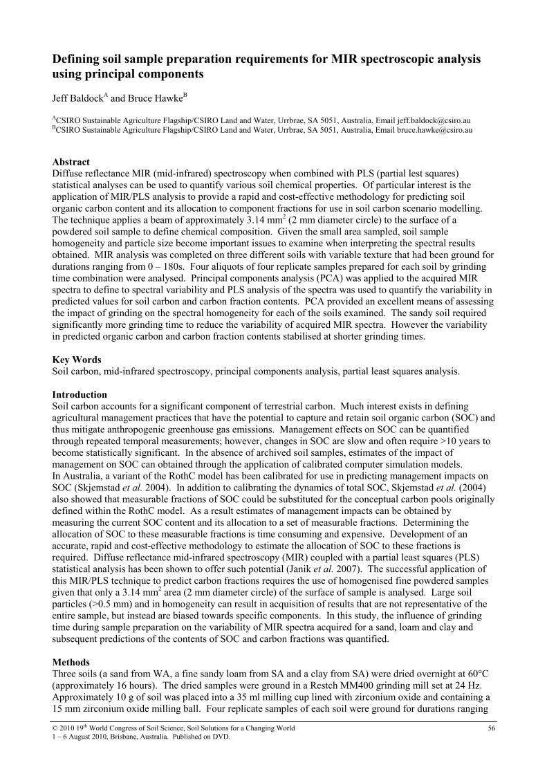
© 2010 19th World Congress of Soil Science, Soil Solutions for a Changing World
1 – 6 August 2010, Brisbane, Australia. Published on DVD. 56
Defining soil sample preparation requirements for MIR spectroscopic analysis
using principal components
Jeff BaldockA and Bruce Hawke
B
ACSIRO Sustainable Agriculture Flagship/CSIRO Land and Water, Urrbrae, SA 5051, Australia, Email [email protected] BCSIRO Sustainable Agriculture Flagship/CSIRO Land and Water, Urrbrae, SA 5051, Australia, Email [email protected]
Abstract Diffuse reflectance MIR (mid-infrared) spectroscopy when combined with PLS (partial lest squares)
statistical analyses can be used to quantify various soil chemical properties. Of particular interest is the
application of MIR/PLS analysis to provide a rapid and cost-effective methodology for predicting soil
organic carbon content and its allocation to component fractions for use in soil carbon scenario modelling.
The technique applies a beam of approximately 3.14 mm2 (2 mm diameter circle) to the surface of a
powdered soil sample to define chemical composition. Given the small area sampled, soil sample
homogeneity and particle size become important issues to examine when interpreting the spectral results
obtained. MIR analysis was completed on three different soils with variable texture that had been ground for
durations ranging from 0 – 180s. Four aliquots of four replicate samples prepared for each soil by grinding
time combination were analysed. Principal components analysis (PCA) was applied to the acquired MIR
spectra to define to spectral variability and PLS analysis of the spectra was used to quantify the variability in
predicted values for soil carbon and carbon fraction contents. PCA provided an excellent means of assessing
the impact of grinding on the spectral homogeneity for each of the soils examined. The sandy soil required
significantly more grinding time to reduce the variability of acquired MIR spectra. However the variability
in predicted organic carbon and carbon fraction contents stabilised at shorter grinding times.
Key Words Soil carbon, mid-infrared spectroscopy, principal components analysis, partial least squares analysis.
Introduction Soil carbon accounts for a significant component of terrestrial carbon. Much interest exists in defining
agricultural management practices that have the potential to capture and retain soil organic carbon (SOC) and
thus mitigate anthropogenic greenhouse gas emissions. Management effects on SOC can be quantified
through repeated temporal measurements; however, changes in SOC are slow and often require >10 years to
become statistically significant. In the absence of archived soil samples, estimates of the impact of
management on SOC can obtained through the application of calibrated computer simulation models.
In Australia, a variant of the RothC model has been calibrated for use in predicting management impacts on
SOC (Skjemstad et al. 2004). In addition to calibrating the dynamics of total SOC, Skjemstad et al. (2004)
also showed that measurable fractions of SOC could be substituted for the conceptual carbon pools originally
defined within the RothC model. As a result estimates of management impacts can be obtained by
measuring the current SOC content and its allocation to a set of measurable fractions. Determining the
allocation of SOC to these measurable fractions is time consuming and expensive. Development of an
accurate, rapid and cost-effective methodology to estimate the allocation of SOC to these fractions is
required. Diffuse reflectance mid-infrared spectroscopy (MIR) coupled with a partial least squares (PLS)
statistical analysis has been shown to offer such potential (Janik et al. 2007). The successful application of
this MIR/PLS technique to predict carbon fractions requires the use of homogenised fine powdered samples
given that only a 3.14 mm2 area (2 mm diameter circle) of the surface of sample is analysed. Large soil
particles (>0.5 mm) and in homogeneity can result in acquisition of results that are not representative of the
entire sample, but instead are biased towards specific components. In this study, the influence of grinding
time during sample preparation on the variability of MIR spectra acquired for a sand, loam and clay and
subsequent predictions of the contents of SOC and carbon fractions was quantified.
Methods Three soils (a sand from WA, a fine sandy loam from SA and a clay from SA) were dried overnight at 60°C
(approximately 16 hours). The dried samples were ground in a Restch MM400 grinding mill set at 24 Hz.
Approximately 10 g of soil was placed into a 35 ml milling cup lined with zirconium oxide and containing a
15 mm zirconium oxide milling ball. Four replicate samples of each soil were ground for durations ranging
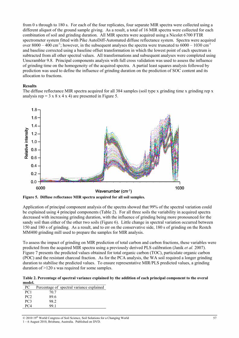
© 2010 19th World Congress of Soil Science, Soil Solutions for a Changing World
1 – 6 August 2010, Brisbane, Australia. Published on DVD. 57
from 0 s through to 180 s. For each of the four replicates, four separate MIR spectra were collected using a
different aliquot of the ground sample giving. As a result, a total of 16 MIR spectra were collected for each
combination of soil and grinding duration. All MIR spectra were acquired using a Nicolet 6700 FTIR
spectrometer system fitted with Pike AutoDiff-Automated diffuse reflectance system. Spectra were acquired
over 8000 – 400 cm-1
; however, in the subsequent analyses the spectra were truncated to 6000 – 1030 cm-1
and baseline corrected using a baseline offset transformation in which the lowest point of each spectrum is
subtracted from all other spectral values. All transformations and subsequent analyses were completed using
Unscrambler 9.8. Principal components analysis with full cross validation was used to assess the influence
of grinding time on the homogeneity of the acquired spectra. A partial least squares analysis followed by
prediction was used to define the influence of grinding duration on the prediction of SOC content and its
allocation to fractions.
Results The diffuse reflectance MIR spectra acquired for all 384 samples (soil type x grinding time x grinding rep x
analysis rep = 3 x 8 x 4 x 4) are presented in Figure 5.
Re
lative in
tensity
Wavenumber (cm-1)6000
0.0
0.2
0.4
0.6
0.8
1.0
1.2
1.4
1.6
1.8
1030
Re
lative in
tensity
Wavenumber (cm-1)6000
0.0
0.2
0.4
0.6
0.8
1.0
1.2
1.4
1.6
1.8
1030
Figure 5. Diffuse reflectance MIR spectra acquired for all soil samples.
Application of principal component analysis of the spectra showed that 99% of the spectral variation could
be explained using 4 principal components (Table 2). For all three soils the variability in acquired spectra
decreased with increasing grinding duration, with the influence of grinding being more pronounced for the
sandy soil than either of the other two soils (Figure 6). Little change in spectral variation occurred between
150 and 180 s of grinding. As a result, and to err on the conservative side, 180 s of grinding on the Restch
MM400 grinding mill used to prepare the samples for MIR analysis.
To assess the impact of grinding on MIR prediction of total carbon and carbon fractions, these variables were
predicted from the acquired MIR spectra using a previously derived PLS calibration (Janik et al. 2007).
Figure 7 presents the predicted values obtained for total organic carbon (TOC), particulate organic carbon
(POC) and the resistant charcoal fraction. As for the PCA analysis, the WA soil required a longer grinding
duration to stabilise the predicted values. To ensure representative MIR/PLS predicted values, a grinding
duration of >120 s was required for some samples.
Table 2. Percentage of spectral variance explained by the addition of each principal component to the overal
model.
PC Percentage of spectral variance explained
PC1 70.7
PC2 89.6
PC3 98.2
PC4 99.1
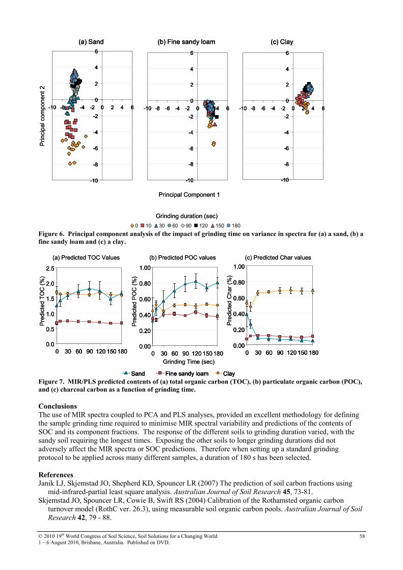
© 2010 19th World Congress of Soil Science, Soil Solutions for a Changing World
1 – 6 August 2010, Brisbane, Australia. Published on DVD. 58
Prin
cip
al co
mpo
ne
nt
2
-10
-8
-6
-4
-2
0
2
4
6
-10 -8 -6 -4 -2 0 2 4 6
(a) Sand
0 10 30 60 90 120 150 180
Grinding duration (sec)
(c) Clay
-10
-8
-6
-4
-2
0
2
4
6
-10 -8 -6 -4 -2 0 2 4 6
(b) Fine sandy loam
-10
-8
-6
-4
-2
0
2
4
6
-10 -8 -6 -4 -2 0 2 4 6
Principal Component 1
Prin
cip
al co
mpo
ne
nt
2
-10
-8
-6
-4
-2
0
2
4
6
-10 -8 -6 -4 -2 0 2 4 6
(a) Sand
-10
-8
-6
-4
-2
0
2
4
6
-10 -8 -6 -4 -2 0 2 4 6
-10
-8
-6
-4
-2
0
2
4
6
-10 -8 -6 -4 -2 0 2 4 6
(a) Sand
0 10 30 60 90 120 150 1800 10 30 60 90 120 150 180
Grinding duration (sec)
(c) Clay
-10
-8
-6
-4
-2
0
2
4
6
-10 -8 -6 -4 -2 0 2 4 6
(c) Clay
-10
-8
-6
-4
-2
0
2
4
6
-10 -8 -6 -4 -2 0 2 4 6
-10
-8
-6
-4
-2
0
2
4
6
-10 -8 -6 -4 -2 0 2 4 6
(b) Fine sandy loam
-10
-8
-6
-4
-2
0
2
4
6
-10 -8 -6 -4 -2 0 2 4 6
(b) Fine sandy loam
-10
-8
-6
-4
-2
0
2
4
6
-10 -8 -6 -4 -2 0 2 4 6
-10
-8
-6
-4
-2
0
2
4
6
-10 -8 -6 -4 -2 0 2 4 6
Principal Component 1
Figure 6. Principal component analysis of the impact of grinding time on variance in spectra for (a) a sand, (b) a
fine sandy loam and (c) a clay.
ClayFine sandy loamSand
(a) Predicted TOC Values
0.0
0.5
1.0
1.5
2.0
2.5
0 30 60 90 120 150 180
Pre
dic
ted T
OC
(%
)
(b) Predicted POC values
0.00
0.20
0.40
0.60
0.80
1.00
0 30 60 90 120 150 180
Grinding Time (sec)
Pre
dic
ted P
OC
(%
)
(c) Predicted Char values
0.00
0.20
0.40
0.60
0.80
1.00
0 30 60 90 120 150 180
Pre
dic
ted C
har
(%)
ClayFine sandy loamSand ClayClayFine sandy loamFine sandy loamSandSand
(a) Predicted TOC Values
0.0
0.5
1.0
1.5
2.0
2.5
0 30 60 90 120 150 180
0.0
0.5
1.0
1.5
2.0
2.5
0 30 60 90 120 150 180
Pre
dic
ted T
OC
(%
)
(b) Predicted POC values
0.00
0.20
0.40
0.60
0.80
1.00
0 30 60 90 120 150 180
0.00
0.20
0.40
0.60
0.80
1.00
0 30 60 90 120 150 180
Grinding Time (sec)
Pre
dic
ted P
OC
(%
)
(c) Predicted Char values
0.00
0.20
0.40
0.60
0.80
1.00
0 30 60 90 120 150 180
0.00
0.20
0.40
0.60
0.80
1.00
0 30 60 90 120 150 180
Pre
dic
ted C
har
(%)
Figure 7. MIR/PLS predicted contents of (a) total organic carbon (TOC), (b) particulate organic carbon (POC),
and (c) charcoal carbon as a function of grinding time.
Conclusions The use of MIR spectra coupled to PCA and PLS analyses, provided an excellent methodology for defining
the sample grinding time required to minimise MIR spectral variability and predictions of the contents of
SOC and its component fractions. The response of the different soils to grinding duration varied, with the
sandy soil requiring the longest times. Exposing the other soils to longer grinding durations did not
adversely affect the MIR spectra or SOC predictions. Therefore when setting up a standard grinding
protocol to be applied across many different samples, a duration of 180 s has been selected.
References Janik LJ, Skjemstad JO, Shepherd KD, Spouncer LR (2007) The prediction of soil carbon fractions using
mid-infrared-partial least square analysis. Australian Journal of Soil Research 45, 73-81.
Skjemstad JO, Spouncer LR, Cowie B, Swift RS (2004) Calibration of the Rothamsted organic carbon
turnover model (RothC ver. 26.3), using measurable soil organic carbon pools. Australian Journal of Soil
Research 42, 79 - 88.
© 2010 19th World Congress of Soil Science, Soil Solutions for a Changing World
1 – 6 August 2010, Brisbane, Australia. Published on DVD. 59
Development of Pedotransfer Functions to Predict Soil Hydraulic Properties in
Golestan Province, Iran
F. Sarmadian and R. Taghizadeh Mehrjardi
Department of Soil Science, College of Agriculture & Natural Resources, University of Tehran, Karaj, 31587-77871, Iran
Abstract The research presented in this paper attempts to develop a more realistic model using multi-layer perceptron
(MLP) and Adaptive neuro-fuzzy inference system (ANFIS) instead of traditional models like multiple linear
regression (MLR) for predicting of infiltration rate and deep percolation. Soil samples were collected from
different horizons of profiles located in the Gorgan Province, North of Iran. Measured soil variables included
texture, organic carbon, water saturation percentage, bulk density, infiltration rate and deep percolation. Then,
MLR, ANFIS and ANN models were employed to develop a pedotransfer function for predicting soil
parameters using easily measurable characteristics of clay, silt, SP, Bd and organic carbon. The performance
of models was evaluated using RMSE. Results showed that the neuro-fuzzy model gives better estimation
than the other techniques for all characteristics. After neuro-fuzzy model, artificial neural network had better
accuracy than multivariate regression.
Key Words Infiltration rate, deep percolation, pedotransfer function.
Introduction In the recent years, the development of prediction methods that use cheap secondary information to spatially
extend sparse and expensive soil measurements has been a sharpening focus of research (Bishop and
McBratney 2001). Several attempts have been made to estimate indirectly soil properties from more easily
measurable and more readily available soil properties such as particle size distribution (sand, silt and clay
content), organic matter or organic carbon content, bulk density, porosity, etc. Such relationships are referred
to as pedo-transfer functions (PTFs) (Mermoud and Xu 2006).
A recent approach to model PTFs is the use of artificial neural networks (ANNs) (Schaap et al. 1998) ANFIS
(Wieland and Wilfried Mirschel 2008). ANN offers a fundamentally different approach for modeling soil
behavior. ANN is an oversimplified simulation of the human brain and composed of simple processing units
referred to as neurons. It is able to learn and generalize from experimental data even if they are noisy and
imperfect. This ability allows this computational system to learn constitutive relationships of materials
directly from the result of experiments. Unlike conventional models, it needs no prior knowledge, or any
constants and/or assumptions about the deformation characteristics of the geomaterials. Other powerful
attributes of ANN models are their flexibility and adaptivity, which play an important role in material
modeling. When a new set of experimental results cannot be reproduced by conventional models, a new
constitutive model or a set of new constitutive equations needs to be developed. However, trained ANN
models can be further trained with the new data set to gain the required additional information needed to
reproduce the new experimental results. These features ascertain the ANN model to be an objective model
that can truly represent natural neural connections among variables, rather than a subjective model, which
assumes variables obeying a set of predefined relations (Banimahd et al. 2005). In brief, a neural network
consists of an input, a hidden, and an output layer all containing “nodes”. The number of nodes in input (e.g.
soil bulk density, soil particle size data and etc) and output (different soil properties) layers corresponds to the
number of input and output variables of the model (Manyame et al. 2007). A type of ANN known as
multilayer perceptron (MLP), which uses a back-propagation training algorithm, is usually used for
generating PTFs (Schaap et al. 1998; Minasny et al. 1999; Minasny and McBratney 2002; Amini et al. 2005).
This network uses neurons whose output is a function of a weighted sum of the inputs.
Since Zadeh (1965) proposed the fuzzy logic approach to describe complicated systems, it has become
popular and been successfully used in various engineering problems, especially on control processes (Barreto-
Neto and Filho 2008). Ralf Wieland and Wilfried Mirschel (2008) a feed forward neural network (NN), a
radial basis function network (RBF) and a trained fuzzy algorithm compared for regional yield estimation of
agricultural crops (winter rye, winter barley).
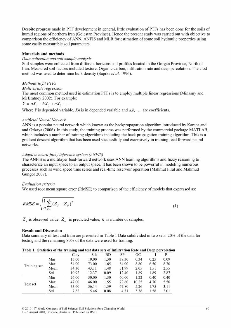
© 2010 19th World Congress of Soil Science, Soil Solutions for a Changing World
1 – 6 August 2010, Brisbane, Australia. Published on DVD. 60
Despite progress made in PTF development in general, little evaluation of PTFs has been done for the soils of
humid regions of northern Iran (Golestan Province). Hence the present study was carried out with objective to
comparison the efficiency of ANN, ANFIS and MLR for estimation of some soil hydraulic properties using
some easily measurable soil parameters.
Materials and methods Data collection and soil sample analysis
Soil samples were collected from different horizons soil profiles located in the Gorgan Province, North of
Iran. Measured soil factors included texture, Organic carbon, infiltration rate and deep percolation. The clod
method was used to determine bulk density (Saprks et al. 1996).
Methods to fit PTFs
Multivariate regression
The most common method used in estimation PTFs is to employ multiple linear regressions (Minasny and
McBratney 2002). For example:
....321 +++= cXbXaXY
Where Y is depended variable, Xn is in depended variable and a,b, …. are coefficients.
Artificial Neural Network
ANN is a popular neural network which known as the backpropagation algorithm introduced by Karaca and
and Ozkaya (2006). In this study, the training process was performed by the commercial package MATLAB,
which includes a number of training algorithms including the back propagation training algorithm. This is a
gradient descent algorithm that has been used successfully and extensively in training feed forward neural
networks.
Adaptive neuro-fuzzy inference system (ANFIS)
The ANFIS is a multilayer feed-forward network uses ANN learning algorithms and fuzzy reasoning to
characterize an input space to an output space. It has been shown to be powerful in modeling numerous
processes such as wind speed time series and real-time reservoir operation (Mahmut Firat and Mahmud
Gungor 2007).
Evaluation criteria
We used root mean square error (RMSE) to comparison of the efficiency of models that expressed as:
∑=
−=n
k
OS ZZn
RMSE1
2)(1
(1)
sZ is observed value, oZ is predicted value, n is number of samples.
Result and Discussion Data summary of test and train are presented in Table 1 Data subdivided in two sets: 20% of the data for
testing and the remaining 80% of the data were used for training.
Table 1. Statistics of the training and test data sets of Infiltration Rate and Deep percolation
Clay Silt BD SP OC I P
Min 15.00 19.00 1.30 38.30 0.34 0.25 0.09
Max 54.00 73.00 1.65 84.00 8.80 6.50 8.70
Mean 34.30 43.11 1.48 51.99 2.05 1.51 2.55 Training set
Std 10.92 12.37 0.09 12.40 1.89 1.89 2.87
Min 26.00 30.00 1.30 60.00 1.22 0.40 0.40
Max 47.00 46.00 1.55 72.60 10.25 4.70 5.50
Mean 33.60 36.14 1.39 67.80 5.26 1.75 3.11 Test set
Std 7.82 5.46 0.08 4.31 3.38 1.58 2.01

© 2010 19th World Congress of Soil Science, Soil Solutions for a Changing World
1 – 6 August 2010, Brisbane, Australia. Published on DVD. 61
Some soil parameters including: clay, silt, Bulk density, water saturation percentage and organic carbon were
input data for prediction of Infiltration rate and Deep percolation. Firs step was to evaluate accuracy of ANN
for predicting known data. So we modeled the ANN for predicting of training data. Results revealed that high
accuracy of ANN. After confirming of performances of ANN, different neurons were examined for achieving
the best neuron for predicting of soil properties. In this stage we used RMSE criteria for determine the best
model. Results showed that for infiltration rate five neurons and for deep percolation two neurons had the
lowest RMSE.
Then, MLR was computed for soil training data set by MINITAB software. These equations were expressed
as:
I = 12.7 - 0.188 Clay - 0.053 silt - 10.3 BD + 0.187 SP - 0.199 OC (1)
P = 37.3 - 0.289 Clay - 0.176 silt - 17.4 BD + 0.130 SP - 0.488 OC (2)
After determining of these equations, performance of MLR was developed for test data set. Results showed
that ANN had better performance in predicting all soil properties than MLR which is in line with the work
done by Amini et al. 2005, Tamari and Wösten (1996), Minasny and McBratney (2002) and Schaap et al.
(1998).
After MLR and ANN, ANFIS model was computed. There are several fuzzy inference engines which can be
utilized for this purpose, which Sugeno and Mamdani are of the most important ones. At this stage, we
compute neuro-fuzzy model for predicting mentioned parameters. The best structure of Neuro-fuzzy model
obtained according to less RMSE. Result of ANFIS, ANN and MR showed in Table 2. As this table
demonstrates ANFIS had the highest accurate for predicting the both parameters.
Table 2. The results of linear regression and neural network-based pedo-transfer functions.
Models Soil parameters RMSE
IR 9.44 Linear regression
DP 7.92
IR 7.24 ANN
DP 6.54
IR 5.78 ANFIS
DP 5.55
Conclusion At present research, we compare applicability and accuracy of three models for prediction of IR and DP.
Results revealed that the ANFIS model gives better estimates than the other techniques. After this model,
ANN had better accuracy than MLR for prediction of mentioned parameters. It is founded that ANFIS and
ANNs had high accuracy for prediction of mentioned parameters but the application of artificial neural
networks and fuzzy systems to real problems should be done with care.
References Amini M, Abbaspour KC, Khademi H, Fathianpour N, Afyuni M, Schulin R (2005) Neural network models
to predict cation exchange capacity in arid regions of Iran. European Journal of Soil Science 56, 551-
559. Banimahd M, Yasrobi SS, Woodward PK (2005) Artificial neural network for stress–strain behavior of sandy
soils: Knowledge based verification. Comput. Geotech. 32, 377–386.
Barreto-Neto AA, Filho CRDS (2008) Application of fuzzy logic to the evaluation of runoff in a tropical
watershed. Environmental Modelling & Software 23, 244-253.
Bishop TFA, McBratney AB (2001) A comparison of prediction methods for the creation of field-extent soil
property maps. Geoderma 103, 149–160.
Karaca F, Ozkaya B (2006) NN-LEAP: A neural network-based model for controlling leachate flow-rate in a
municipal solid waste landfill site. Environmental Modelling & Software 21, 1190-1197.
Mahmut F, Mahmud G (2007) River flow estimation using adaptive neuro fuzzy inference system.
Mathematics and Computers in Simulation 75, 87–96.
Manyame C, Morgan CL, Heilman JL, Fatondji D, Gerard B, Payne WA (2007). Modeling hydraulic
properties of sandy soils of Niger using pedotransfer functions. Geoderma 141, 407–415.
Merdun H, Cınar O, Meral R, Apan M (2006). Comparison of artificial neural network and regression

© 2010 19th World Congress of Soil Science, Soil Solutions for a Changing World
1 – 6 August 2010, Brisbane, Australia. Published on DVD. 62
pedotransfer functions for prediction of soil water retention and saturated hydraulic conductivity. Soil &
Tillage Research 90, 108–116.
Minasny B, McBratney AB, Bristow KL (1999) Comparison of different approaches to the development of
pedotransfer functions for water-retention curves. Geoderma 93, 225–253.
Minasny B, McBratney AB (2002) The neuro-m methods for fitting neural network parametric pedotransfer
functions. Soil Science Society of America Journal 66, 352–361.
Schaap MG, Leij FJ, van Genuchten MTh (1998) Neural network analysis for hierarchical prediction of soil
hydraulic properties. Soil Science Society of America Journal 62, 847–855.
Schaap MG, Leij FJ (1998) Using neural networks to predict soil water retention and soil hydraulic
conductivity. Soil & Tillage Research 47, 37–42.
Sparks DL, Page AL, Helmke PA, Leoppert RH, Soltanpour PN, Tabatabai MA, Johnston GT, Summer ME
(1996) Methods of soil analysis. (Soil Sci. Soc. Of Am., Madison, Wisconsin).
Tamari S, Wosten JHM, Ruiz-Suarez JC (1996) Testing an artificial neural network for predicting soil
hydraulic conductivity. Soil Science Society of America Journal 60, 1732–1741.
Wieland R, Mirschel W (2008) Adaptive fuzzy modeling versus artificial neural networks. Environmental
Modelling & Software 23, 215-224.
© 2010 19th World Congress of Soil Science, Soil Solutions for a Changing World
1 – 6 August 2010, Brisbane, Australia. Published on DVD. 63
Electromagnetic Imaging of Prior Stream Channels using a DUALEM-421 and
Inversion
Kira BruzgulisA, John Triantafilis
A and Fernando Monteiro Santos
B
AFaculty of Science, School of Biological Earth and Environmental Sciences, University of New South Wales, Sydney, NSW,
Australia, Email [email protected] BUniversidade de Lisboa, Instituto Don Luís Laboratório Associado, C8, 1749-016 Lisboa, Portugal
Abstract Prior stream channels occupy 15% of the clay alluvial fields used for irrigated cotton production in the lower
Gwydir Valley in north-western NSW. They act as significant hydrological features offering pathways for
deep draining water to interact with buried palaeochannels. We need to map the connectivity and spatial
extent of these formations to improve the scientific understanding of the associated hydrological processes in
this region. In this paper we explore this by first measuring the apparent electrical conductivity (σa) of the
soil with a DUALEM-421. Subsequently, we employ 1-dimensional (1-D) inversion algorithms with 2-
dimensional (2-D) smoothness constraints to predict the true electrical conductivity (σ) using DUALEM-2d
(partial solution) and DUALEM-2d-Full (full solution). The σ models obtained are compared with soil data
(including particle size fractions, soil texture, EC1:5 and CEC) collected across the field. All σ models
generally reflect the soil properties which characterise the physiographic units of a prior stream channel and
the clay alluvial plain. However, the relationship between the measured soil properties and estimated σ is
weak and further research is needed to achieve better relationships.
Key Words Prior stream channels, DUALEM-421, electromagnetic (EM) induction, inversion.
Introduction Prior stream channels occupy 15 % of the clay alluvial landscapes that are used extensively for irrigated
cotton production in the lower Gwydir Valley in north-western New South Wales, Australia (Needham
1991). In order to improve the scientific understanding of the hydrological processes across this landscape,
especially where the management of water is crucial and climatic models and trends suggest that rainfall is in
decline (Kothavala 1999), there is a need for better representation and ability to map the connectivity and
spatial extent of prior stream channels and palaeochannels. Electromagnetic (EM) induction is a cost
effective and proximal geophysical method that has successfully been employed in measuring both the areal
(Triantafilis et al. 2003) and stratigraphic (Vervoort and Annen 2006) distribution of apparent electrical
conductivity (σa – mS/m) of prior stream channels within the current study site. The aim of this study is to
use σa data collected by a DUALEM-421 to infer the spatial distribution of soil properties and soil particle
size fractions related to σa across a prior stream channel in an irrigated cotton field in the lower Gwydir
valley. This is achieved by using two inversion programs, DUALEM-2d and DUALEM-2d-Full, that
estimates the true electrical conductivity (σ) of the soil at discrete increments. These programs are modified
versions of the nonlinear smoothness constrained inversion algorithm described in (Santos 2004) and
incorporate a damping factor (the Lagrange parameter) that is used to control the balance between the data fit
and its closeness to the initial model.
Materials and Methods The study site is located within Field 11 of Auscott ‘Midkin’, a large irrigated cotton farm situated
approximately 20 km away from Moree in the lower Gwydir Valley. A large prior stream channel is located
in Field 11. It is most prominent in the southern end of the field wherein it dissipates as it extends to the
north. The DUALEM-421 is an EM instrument which operates at 9.1 kHz and consists of one transmitting
coil and three pairs of receiving coils spaced 1, 2 and 4 m apart from the transmitting coil. Each coil pair
consists of a coil with horizontal windings forming a horizontal coplanar (HCP) array and a coil with vertical
windings forming a perpendicular (PRP) array. Each coil array measures the apparent electrical conductivity
(σa) of the soil for six different depths of exploration (DOEs) relating to the geometry of the instrument (i.e.
coil spacing and orientation) and the frequency of operation. The HCP arrays measure the σa (Hcon – mS/m)
of the soil from 0 to 1.5 m (1mHcon), 0 to 3 m (2mHcon) and 0 to 6 m (4mHcon). The PRP arrays measure
the σa (Pcon – mS/m) of the soil from 0 to 0.6 m (1mPcon), 0 to 1.2 m (2mPcon), and 0 to 2.4 m (4mPcon).
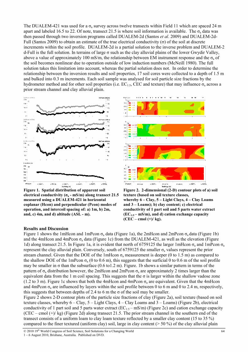
© 2010 19th World Congress of Soil Science, Soil Solutions for a Changing World
1 – 6 August 2010, Brisbane, Australia. Published on DVD. 64
The DUALEM-421 was used for a σa survey across twelve transects within Field 11 which are spaced 24 m
apart and labeled 16.5 to 22. Of note, transect 21.5 is where soil information is available. The σa data was
then passed through two inversion programs called DUALEM-2d (Santos et al. 2009) and DUALEM-2d-
Full (Santos 2009) to obtain an estimate of the true electrical conductivity (σ) of the soil at discrete
increments within the soil profile. DUALEM-2d is a partial solution to the inverse problem and DUALEM-2
d-Full is the full solution. In terrains of large σ such as the clay alluvial plains of the lower Gwydir Valley,
above a value of approximately 100 mS/m, the relationship between EM instrument response and the σa of
the soil becomes nonlinear due to operation outside of low induction numbers (McNeill 1980). The full
solution takes this limitation into account, whereas the partial solution does not. In order to determine the
relationship between the inversion results and soil properties, 17 soil cores were collected to a depth of 1.5 m
and bulked into 0.3 m increments. Each soil sample was analysed for soil particle size fractions by the
hydrometer method and for other soil properties (i.e. EC1:5, CEC and texture) that may influence σa across a
prior stream channel and clay alluvial plain.
Figure 1. Spatial distribution of apparent soil
electrical conductivity (σa - mS/m) along transect 21.5
measured using a DUALEM-421 in horizontal
coplanar (Hcon) and perpendicular (Pcon) modes of
operation, and intercoil spacing of: a) 1m, b) 2m,
and, c) 4m, and d) altitude (ASL - m).
Figure 2. 2-dimensional (2-D) contour plots of a) soil
texture (based on soil texture classes,
whereby 6 – Clay, 5 – Light Clays, 4 – Clay Loams
and 3 – Loams); b) clay content; c) electrical
conductivity of 1 part soil and 5 parts water extract
(EC1:5 – mS/m), and d) cation exchange capacity
(CEC – cmol (+)/ kg).
Results and Discussion Figure 1 shows the 1mHcon and 1mPcon σa data (Figure 1a), the 2mHcon and 2mPcon σa data (Figure 1b)
and the 4mHcon and 4mPcon σa data (Figure 1c) from the DUALEM-421, as well as the elevation (Figure
1d) along transect 21.5. In Figure 1a, it is evident that north of 6759125 the larger 1mHcon σa and 1mPcon σa
represent the clay alluvial plain. Conversely, south of 6759125 the smaller σa values represent the prior
stream channel. Given that the DOE of the 1mHcon σa measurement is deeper (0 to 1.5 m) as compared to
the shallow DOE of the 1mPcon σa (0 to 0.6 m), this suggests that the surficial 0 to 0.6 m of the soil profile
may be smaller in σ than the subsurface (0.6 to1.2 m). Figure. 1b shows a similar pattern in terms of the
pattern of σa distribution however, the 2mHcon and 2mPcon σa are approximately 2 times larger than the
equivalent data from the 1 m coil spacing. This suggests that the σ is larger within the shallow vadose zone
(1.2 to 3 m). Figure 1c shows that both the 4mHcon and 4mPcon σa are equivalent. Given that the 4mHcon
and 4mPcon σa are influenced by layers within the soil profile between 0 to 6 m and 0 to 2.4 m, respectively,
this suggests that between depths of 2.4 to 6 m the σ of the soil may be smaller.
Figure 2 shows 2-D contour plots of the particle size fractions of clay (Figure 2a), soil texture (based on soil
texture classes, whereby 6 – Clay, 5 – Light Clays, 4 – Clay Loams and 3 – Loams) (Figure 2b), electrical
conductivity of 1 part soil and 5 parts water extract (EC1:5 – mS/m) (Figure 2c) and cation exchange capacity
(CEC – cmol (+)/ kg) (Figure 2d) along transect 21.5. The prior stream channel in the southern end of the
transect consists of a uniform loam to clay loam texture reflected by a smaller clay content (15 to 35 %)
compared to the finer textured (uniform clay) soil, large in clay content (> 50 %) of the clay alluvial plain
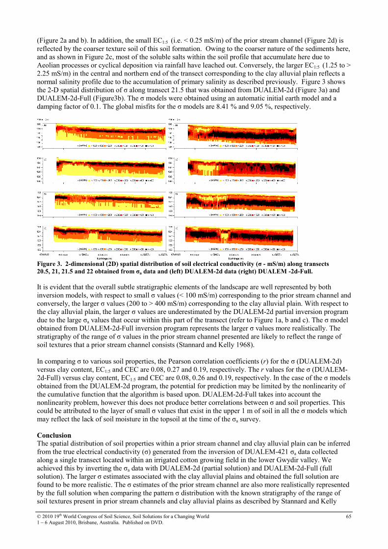
© 2010 19th World Congress of Soil Science, Soil Solutions for a Changing World
1 – 6 August 2010, Brisbane, Australia. Published on DVD. 65
(Figure 2a and b). In addition, the small EC1:5 (i.e. < 0.25 mS/m) of the prior stream channel (Figure 2d) is
reflected by the coarser texture soil of this soil formation. Owing to the coarser nature of the sediments here,
and as shown in Figure 2c, most of the soluble salts within the soil profile that accumulate here due to
Aeolian processes or cyclical deposition via rainfall have leached out. Conversely, the larger EC1:5 (1.25 to >
2.25 mS/m) in the central and northern end of the transect corresponding to the clay alluvial plain reflects a
normal salinity profile due to the accumulation of primary salinity as described previously. Figure 3 shows
the 2-D spatial distribution of σ along transect 21.5 that was obtained from DUALEM-2d (Figure 3a) and
DUALEM-2d-Full (Figure3b). The σ models were obtained using an automatic initial earth model and a
damping factor of 0.1. The global misfits for the σ models are 8.41 % and 9.05 %, respectively.
Figure 3. 2-dimensional (2D) spatial distribution of soil electrical conductivity (σ - mS/m) along transects
20.5, 21, 21.5 and 22 obtained from σa data and (left) DUALEM-2d data (right) DUALEM -2d-Full.
It is evident that the overall subtle stratigraphic elements of the landscape are well represented by both
inversion models, with respect to small σ values (< 100 mS/m) corresponding to the prior stream channel and
conversely, the larger σ values (200 to > 400 mS/m) corresponding to the clay alluvial plain. With respect to
the clay alluvial plain, the larger σ values are underestimated by the DUALEM-2d partial inversion program
due to the large σa values that occur within this part of the transect (refer to Figure 1a, b and c). The σ model
obtained from DUALEM-2d-Full inversion program represents the larger σ values more realistically. The
stratigraphy of the range of σ values in the prior stream channel presented are likely to reflect the range of
soil textures that a prior stream channel consists (Stannard and Kelly 1968).
In comparing σ to various soil properties, the Pearson correlation coefficients (r) for the σ (DUALEM-2d)
versus clay content, EC1:5 and CEC are 0.08, 0.27 and 0.19, respectively. The r values for the σ (DUALEM-
2d-Full) versus clay content, EC1:5 and CEC are 0.08, 0.26 and 0.19, respectively. In the case of the σ models
obtained from the DUALEM-2d program, the potential for prediction may be limited by the nonlinearity of
the cumulative function that the algorithm is based upon. DUALEM-2d-Full takes into account the
nonlinearity problem, however this does not produce better correlations between σ and soil properties. This
could be attributed to the layer of small σ values that exist in the upper 1 m of soil in all the σ models which
may reflect the lack of soil moisture in the topsoil at the time of the σa survey.
Conclusion The spatial distribution of soil properties within a prior stream channel and clay alluvial plain can be inferred
from the true electrical conductivity (σ) generated from the inversion of DUALEM-421 σa data collected
along a single transect located within an irrigated cotton growing field in the lower Gwydir valley. We
achieved this by inverting the σa data with DUALEM-2d (partial solution) and DUALEM-2d-Full (full
solution). The larger σ estimates associated with the clay alluvial plains and obtained the full solution are
found to be more realistic. The σ estimates of the prior stream channel are also more realistically represented
by the full solution when comparing the pattern σ distribution with the known stratigraphy of the range of
soil textures present in prior stream channels and clay alluvial plains as described by Stannard and Kelly

© 2010 19th World Congress of Soil Science, Soil Solutions for a Changing World
1 – 6 August 2010, Brisbane, Australia. Published on DVD. 66
(1968). The calibration information, specifically the CEC, EC1:5 and soil textural data (indicating a normal
salinity profile in the clay alluvial plain) from the soil cores generally reflects the distribution of σ along
transect 21.5. Specifically, small subsurface σ (0 to 200 mS/m) represents the smaller CEC, EC1:5 and coarser
textures (i.e. sandy loams) of the prior stream channels. Conversely, larger values of σ (> 400 mS/m)
characterise the finer textured (i.e. medium to heavy clays) and slightly larger EC1:5 of the root zone soil
properties of the clay alluvial plain. Whist the σ models are able to generally represent the soil types, the
potential to use σ to predict soil properties is limited. The lack of statistical correlation is attributed to a layer
of small σ values within the upper 1 m of the soil profile that may be affected by low moisture content in the
topsoil at the time of the σa survey. Follow up research should be carried out in more favourable conditions
(i.e. soon after irrigation or heavy rainfall) to determine the influence of soil moisture.
References Kothavala Z (1999) The duration and severity of drought over eastern Australia simulated by a coupled
oceanatmosphereGCM with a transient increase in CO2. Environmental Modelling and Software,
14(4), 243-252.
McNeill JD (1980) Electromagnetic Terrain Conductivity Measurement at Low Induction Numbers.
Technical Note TN6, Geonics Limited, Mississauga, Ontario Canada.
Needham P (1991) The extent of degraded heavy clays and associated soils in north-western New South
Wales, Department of Conservation and Land Management, Soil Conservation Service, Inverell
Research Service Centre, New South Wales, Australia.
Santos FAM (2004) 1-D laterally constrained inversion of EM34 profiling data. Journal of Applied
Geophysics 56, 123-134.
Santos FAM (2009) DUALEM-2D-Full, personal communication.
Santos FAM, Triantafilis J, Bruzgulis KE, Roe JAE (2009) Inversion of DUALEM-421 profiling data using
a 1-D laterally constrained algorithm. Vadose Zone Journal, submitted.
Stannard ME, Kelly ID (1968) Irrigation potential of the lower Gwydir valley, Water Conservation and
Irrigation Commission, New South Wales, Australia.
Triantafilis J, Huckel AI, Odeh IOA (2003) Field-scale assessment of deep drainage risk. Irrigation Science
21(4), 183-192.
Vervoort RW, Annen YL (2006) Palaeochannels in northern New South Wales: inversion of electromagnetic
induction data to infer hydrologically relevant stratigraphy. Australian Journal of Soil Research 44,
35-45.
© 2010 19th World Congress of Soil Science, Soil Solutions for a Changing World
1 – 6 August 2010, Brisbane, Australia. Published on DVD. 67
Field measurement of root density and soil organic carbon content using soil
spectral reflectance
Mike Hedley A, Bambang Kusumo
AC, Carolyn Hedley
B and Mike Tuohy
A.
AInstitute of Natural Resources, College of Sciences, Massey University, Private Bag 11-222, Palmerston North, New Zealand, BLandcare Research, Private Bag 11-052, Palmerston North, New Zealand , CDepartment of Soil Science, Faculty of Agriculture, University of Mataram, Jl. Majapahit 62, Mataram 83125, Lombok, Indonesia.
Abstract This paper summarizes the development of a proximal sensing technique used to predict root density, soil
carbon (C) and soil nitrogen (N) content from the visible and near-infrared (Vis-NIR) spectral reflectance of
soil cores. The techniques were evaluated at two sites in permanent pasture on contrasting soils (an
Allophanic soil and a Fluvial Recent soil) and at two sites within a field of 90-day-old maize silage;
Kairanga silt loam and fine sandy loam (Recent/Orthic Gley Soils) in Manawatu region, New Zealand. A
portable field spectrometer with a modified soil probe was used to acquire reflectance spectra (350-2500 nm)
from horizontal surfaces of soil cores. After scanning, thin soil slices were taken at each depth for root
density measurement and soil C and nitrogen N. Calibration models developed using partial least squares
regression (PLSR) between the first derivative of soil reflectance and the reference data were able to
accurately predict the soil profile root density, and soil C and N concentration for all soils. Predicted root
densities were not strongly autocorrelated to soil C values, indicating that root density can be predicted
independently from soil C. This research has identified a potential method for assessing root densities in field
soils enabling study of their role in soil organic matter synthesis.
Key Words Carbon, nitrogen, near infrared, root density, maize, pasture.
Introduction Pasture rotations in mixed farming systems have long been known to build soil organic matter (SOM) and
create desirable soil structural features for seedbed preparation, drainage and aeration. The amount of SOM
in pastoral soil is closely related to net productivity of roots, which is determined by previous soil and
pasture management history (Nie et al. 1997) and type and stage of growth of the pasture (Fisher et al.
2007). The patterns of carbon (C) sequestration in both arable and pasture soils correlate well to plant root
density and turnover times (Rees et al. 2005). Deeper root systems have the potential to sequester carbon
(Smith 2004) deeper in the soil profile, where root turnover times can be slower. Organic carbon stored
deeper in soil can slow the return of CO2 to the atmosphere. Soil organic carbon stored deeper than 0.2 m and
below 2 m can have residence times of 1000-2000 and 9000-13 000 years, respectively (Follet et al. 2003).
There are other desirable features of deeper rooting plants. Plants with deeper, denser root systems have the
potential to increase water use efficiency by optimising the use of subsoil water, and to recapture nitrate that
would have leached past shallower root systems (Crush et al. 2007; Dunbabin et al. 2003). To exploit these
opportunities crop cultivars that express deeper and denser rooting characteristics will need to be identified
and then evaluated in field trials. Current common methods of measuring root density are the profile wall
(Böhm 1979) and soil corer methods (Escamilla et al. 1991). Both require separation of roots and soil, which
is a tiresome procedure, followed by root length measurement by the line intersect method (Newman 1966).
Recently (Kusumo et al. 2009) used Vis-NIR reflectance spectroscopy to successfully predict, ryegrass root
density in a glasshouse experiment. Sophisticated software (multivariate analysis) has allowed, reflectance
spectra from soil to be calibrated against measured soil properties and the calibrations used to simultaneously
predict several soil properties, such as total C, organic C (e.g. Chang and Laird 2002, Kusumo et al. 2008),
total N, CEC and moisture (Malley and Martin 2003). Plants roots contribute directly to the reflectance
bands associated with water and organic matter but roots as an intrusive property of soils mask other
chromophores, such as, hydrous iron and aluminium oxides, and clays In this paper we summarize our recent
research into improving the ability to predict root density in pasture and cropped soils from Vis-NIR spectral
reflectance acquired from soil cores in the field.
Methods
Sites, soils and vegetation The pasture root density assessment was undertaken at two permanent pasture sites (23.5 km apart): the first

© 2010 19th World Congress of Soil Science, Soil Solutions for a Changing World
1 – 6 August 2010, Brisbane, Australia. Published on DVD. 68
on Ramiha silt loam (Allophanic soil, Andic Dystrochrept derived from loess and andesitic ash) and the
second on Manawatu fine sandy loam (Fluvial Recent soil, Dystric Fluventic Eutrochrept derived from
greywacke alluvium) in the Manawatu region, New Zealand (Hewitt 1998). The permanent ryegrass (Lolium
perenne L) and white clover (Trifolium repens L) dominant pastures at both sites had been present for more
than 20 years. The maize root density assessment was conducted on the day of harvest of a 90 day old maize
crop. Two sites on the Kairanga soil series (Recent/Orthic Gley Soils) were chosen in the same field. At one
site, the soil was dominantly silt loam and at the second site fine sandy loam in texture.
Acquiring spectral reflectance At the pasture site a total of 18 soil cores, 10 m apart from each other, were collected from each site and cut
into three depths (at 15, 30 and 60 mm), providing 54 samples at each site and a total of 108 soil samples.
Reflectance spectra (350-2500 nm) were acquired in situ from the freshly cut surfaces using a purpose built
soil probe attached by fibre optic cable to a field spectroradiometer (ASD FieldSpecPro, Boulder, Colorado,
USA). A 3-mm soil slice (slice A) was collected at each surface, put in a sealed plastic bag and stored as
field moist at 4o C for no more than three days before root densities were measured using the wet sieve
method (Kusumo et al. 2009). Root density was expressed as mg dry root g-1
dry soil. A further 3-mm soil
slice (slice B) was collected; part was used for determining dry soil weight and soil moisture content (oven
dry at 105o C) and part was air dried and analysed for total C and N using a Leco FP-2000 CNS analyser
(LECO Corp., St Joseph, MI, USA).
At each of the two maize sites, three replicate soil cores were taken at 0, 15 and 30 cm distance from the
maize stem towards the centre of the 60 cm row. The distance between each replicate was 40 cm. A soil core
was sectioned at 5 depths (7.5, 15, 30, 45, and 60 cm) and at each depth the soil reflectance spectra was
acquired in situ as describe above. A 1.5 cm soil slice (slice A) was taken above the cut surface to obtain root
mass reference data (using wet sieve laboratory root measurement). Another 1.5 cm soil slice (slice B) was
taken air-dried and analysed for total soil C and N determinations and water content measurement.
Standing biomass
On the day of coring the pasture biomass cover was estimated to be approximately 1500kgDM/ha. Biomass
data of maize stem and cob were collected one day before silage harvesting. Stem and cob dry matter values
were obtained by drying them at 60oC for 12 days.
Spectral data processing and statistical analysis
The spectral data were pre-processed (for details see Kusumo et al. 2009) and first derivatives of 5-nm
spaced data calculated using SpectraProc V 1.1 software (Hueni and Tuohy 2006). The first derivative data
were imported to Minitab 14 (MINITAB Inc. 2003) for principal component analysis (PCA) and partial least
squares regression (PLSR) analysis. Prior to (PLSR) analysis, a PCA was conducted on the first derivative of
the spectral data. A score plot of the first two components (PC1 and PC2) of the PCA analysis was used to
select data for calibration and validation sets
Calibration models were developed by using PLSR to fit the reference data (root density, soil C and N) to
pre-processed spectral data. The accuracy of the PLSR calibration models was tested internally by using a
leave-one-out cross-validation procedure and when sample numbers permitted, externally using a separate
validation sample set.
The best prediction models were shown by the smallest standard deviation of the difference between the
measured and the predicted soil property values (RMSE, calculated from cross-validation is termed
RMSECV and from separate validation is termed RMSEP) and the largest ratio of prediction to deviation
(RPD), the largest ratio of the range of measured values of soil properties to the RMSE (RER) , and the
largest r2 (for more detailed explanation see Kusumo et al. 2009)
Results Pasture soils
Mean root density decreased significantly with depth from 12.4 and 22.5 mg/g soil at 15 mm to 3.2 to 2.6
mg/g soil at 60 mm, both in the Ramiha and the Manawatu soil respectively. If the average amount of root
mass in the 0 – 60 mm depth is expressed per hectare, the total root dry mass was 3642 and 9353 kg DM/ ha
in the Ramiha (Andic Dystrochrept) and the Manawatu soil (Dystric Fluventic Eutrochrept), respectively,
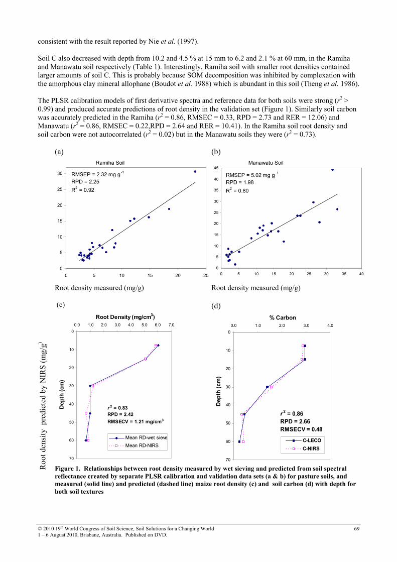
© 2010 19th World Congress of Soil Science, Soil Solutions for a Changing World
1 – 6 August 2010, Brisbane, Australia. Published on DVD. 69
consistent with the result reported by Nie et al. (1997).
Soil C also decreased with depth from 10.2 and 4.5 % at 15 mm to 6.2 and 2.1 % at 60 mm, in the Ramiha
and Manawatu soil respectively (Table 1). Interestingly, Ramiha soil with smaller root densities contained
larger amounts of soil C. This is probably because SOM decomposition was inhibited by complexation with
the amorphous clay mineral allophane (Boudot et al. 1988) which is abundant in this soil (Theng et al. 1986).
The PLSR calibration models of first derivative spectra and reference data for both soils were strong (r2 >
0.99) and produced accurate predictions of root density in the validation set (Figure 1). Similarly soil carbon
was accurately predicted in the Ramiha (r2 = 0.86, RMSEC = 0.33, RPD = 2.73 and RER = 12.06) and
Manawatu (r2 = 0.86, RMSEC = 0.22,RPD = 2.64 and RER = 10.41). In the Ramiha soil root density and
soil carbon were not autocorrelated (r2 = 0.02) but in the Manawatu soils they were (r
2 = 0.73).
(a) (b)
Root density measured (mg/g)
(c)
r2 = 0.83
RPD = 2.42
RMSECV = 1.21 mg/cm3
0
10
20
30
40
50
60
70
0.0 1.0 2.0 3.0 4.0 5.0 6.0 7.0
Root Density (mg/cm3)
Depth (cm)
Mean RD-wet sieve
Mean RD-NIRS
Root density measured (mg/g)
(d)
r2 = 0.86
RPD = 2.66
RMSECV = 0.48
0
10
20
30
40
50
60
70
0.0 1.0 2.0 3.0 4.0
% Carbon
Depth (cm)
C-LECO
C-NIRS
Root
den
sity
p
redic
ted b
y N
IRS
(m
g/g
)
Figure 1. Relationships between root density measured by wet sieving and predicted from soil spectral
reflectance created by separate PLSR calibration and validation data sets (a & b) for pasture soils, and
measured (solid line) and predicted (dashed line) maize root density (c) and soil carbon (d) with depth for
both soil textures
Manawatu Soil
RMSEP = 5.02 mg g -1
RPD = 1.98 R 2 = 0.80
0
5
10
15
20
25
30
35
40
45
0 5 10 15 20 25 30 35 40
Ramiha Soil
RMSEP = 2.32 mg g-1
RPD = 2.25 R 2 = 0.92
0
5
10
15
20
25
30
0 5 10 15 20 25

© 2010 19th World Congress of Soil Science, Soil Solutions for a Changing World
1 – 6 August 2010, Brisbane, Australia. Published on DVD. 70
Maize soils
Root density (Figure 1c) was higher in the top soil (15 cm depth) and decreased with depth and decreased
with distance from the plant stem (in the silt loam soil) but in the fine sandy loam, highest root densities were
found 15 cm distance from the plant stem (data not shown) . Soil carbon also decreased with depth (Figure
1d). Both root density and soil carbon were accurately predicted from the PLSR calibration model developed
using the first derivative of soil spectral reflectance (Figure 1 c & d). Root density could be predicted
independently of soil carbon (data not shown).
Conclusion Our results show that Vis-NIR spectroscopy can be used for prediction of pasture and maize root density and
soil carbon in the field. Accurate PLSR calibration models can be developed from a small calibration set of
field-acquired spectra from a soil slice with known reference root density and soil carbon data. The
calibration models can be used to predict the carbon and root densities in a larger population of acquired
spectral data. This approach can reduce the number of samples that must be measured for root density and
soil carbon, especially when dealing with large sample sets (e.g. for mapping purposes).
References Böhm W (1979) 'Methods of studying root systems.' (Springer: New York).
Boudot JP, Bel Hadi Brahim A, Chone T (1988) Dependence of carbon and nitrogen mineralization rates
upon amorphous metallic constituents and allophanes in highland soils. Geoderma 42, 245-260.
Chang CW, Laird DA (2002) Near-infrared reflectance spectroscopic analysis of soil C and N. Soil Science
167, 110-116.
Crush JR, Easton HS, Waller JE, Hume DE, Faville MJ (2007) Genotypic variation in patterns of root
distribution, nitrate interception and response to moisture stress of a perennial ryegrass (Lolium perenne
L.) mapping population. Grass and Forage Science 62, 256-273.
Dunbabin V, Diggle A, Rengel Z (2003) Is there an optimal root architecture for nitrate capture in leaching
environment? Plant, Cell and Environment 26, 835-844.
Escamilla JA, Comerford NB, Neary DG (1991) Soil core-break method to estimate pine root distribution.
Soil Science Society of America Journal 55, 1722-1726.
Fisher MJ, Braz SP, Dos Santos RSM, Urquiaga S, Alves BJR, Roddey RM (2007) Another dimension to
grazing systems: Soil carbon. Tropical Grasslands 41, 65-83.
Follet RF, Leavitt SW, Kimble JM, Pruessner EG (2003) Paleoenvironmental inferences from δ13C of soil
organic C in 14C-dated profiles in the U.S.Great Plains. In 'XVI INQUA Congress, Reno, NV, 23-30
July, 2003'. (Ed. DA McGilloway).
Hewitt AE (1998) New Zealand Soil Classification. Landcare Research Science Series No. 1. Manaki
Whenua Press, Lincoln, Canterbury. , New Zealand.
Hueni A, Tuohy M (2006) Spectroradiometer data structuring, pre-processing and analysis - An IT based
approach. Journal of Spatial Science 51, 93-102.
Kusumo BH, Hedley CB, Hedley MJ, Hueni A, Tuohy MP, Arnold GC (2008) The use of diffuse reflectance
spectroscopy for in situ carbon and nitrogen analysis of pastoral soils. Australian Journal of Soil
Research 46, 623-635.
Kusumo BH, Hedley MJ, Hedley CB, Hueni A, Arnold GC, Tuohy MP (2009) The use of Vis-NIR spectral
reflectance for determining root density: evaluation of ryegrass roots in a glasshouse trial. European
Journal of Soil Science 60, 22-32.
Malley DF, Martin PD (2003) The use of near-infrared spectroscopy for soil analysis. In ‘Tools for Nutrient
and Pollutant Management: Application to Agriculture and Environmental Quality’. (Eds L.D. Currie &
J.A. Hanly) pp. 371-404. (Fertilizer and Lime Research Centre, Massey University, Palmerston North. ,
New Zealand).
MINITAB Inc. (2003) MINITAB Statistical Software. Minitab Inc., State College, PA.
Nie ZN, Mackay AD, Valentine I, Barker DJ, Hodgson J (1997) Influence of pastoral fallow on plant root
growth and soil physical and chemical characteristics in a hill pasture. Plant and Soil 197, 201-208.
Smith P (2004) Carbon sequestration in croplands: The potential in Europe and the global context. European
Journal of Agronomy 20, 229-236.
Theng BKG, Churchman GJ, Newman RH (1986) The occurrence of interlayer clay-organic complexes in
two New Zealand soils. Soil Science 142, 262-266.
© 2010 19th World Congress of Soil Science, Soil Solutions for a Changing World
1 – 6 August 2010, Brisbane, Australia. Published on DVD. 71
ICP determination of phosphorous in soils and plants
Krasimir IvanovA, Penka Zaprjanova
B, Violina Angelova
A, Georgi Bekjarov
C and Lilko Dospatliev
A
ADepartment of Chemistry, Agricultural University, Plovdiv, Bulgaria, Email [email protected] B Institute of Tobacco and Tobacco Products, Plovdiv, Bulgaria, Email [email protected] CRegional center for scientific and applied services, Plovdiv, Bulgaria, Email [email protected]
Abstract The purpose of our study is to evaluate the appropriateness of an ICP–method for the determination of total
phosphorus content in soils and plants after complete decomposition by acid mixtures. Three certified soil
samples corresponding to two main soil types in Bulgaria and Polish reference material CTA-VTL-2
(Virginia tobacco leaves) were used in the study. It was established that ICP is a fast and correct method for
phosphorus determination in plant materials. We have to use a standard supplement method in order to
obtain correct results for soil samples.
Key Words Phosphorous determination, ICP, soils, plants
Introduction The correct determination of phosphorus content in soils and plants is extremely important for agricultural
science and practice. Phosphorus participates in a number of processes determining the growth, development
and the productivity of the plant: formation of cell nucleus and cell multiplication, synthesis of lipids and
specific proteins, transmission of hereditary properties, breathing and photosynthesis, energy transmission
from richer to poorer energetic compounds, etc. It is very important to know the phosphorus status of soils to
determine the necessity for phosphorus fertilizer use. Phosphorus is known to be unique for its sensitivity
and stability as a human activity indicator. Its content in soil represents a great interest to archaeologists,
giving them information on type and intensity of human activity. Total phosphorus measurement gives
quantitative results in contrast to mobile phosphorus and represents the best indicator for variation caused by
human activity.
During the last year soil and plant laboratories have moved from colorimetry to inductively coupled plasma
(ICP) spectrometry to quantify phosphorous in soil and plants (Sicoria et al. 2005). The main reason is the
increasing critical attitude to the colorimetric measurement due to the significant interference problems upon
Р determination in soils and plants, as well as the advantages of ICP–method related to the fast measurement
and the opportunity to simultaneously determine the main part of the macro-and microelements, contained in
soils and plants. Its adaptation and priority for soil status evaluation is not trouble-free due to controversial
results when compared to the colorimetric method. We have expanded the studies in this sphere to obtain
more experimental results related to sample preparation methods and soil diversity. Several profound studies
comparing both methods for determination of total and mobile phosphorus in various soils are known. Upon
the test falling within the scope of North American Proficiency Testing (NAPT) program conducted in 2001
and 2002, 18 laboratories used the spectrophotometric method and 34 laboratories used the ICP–method
(Sicoria et al. 2005). In 40 samples ICP values for phosphorus, extracted by Mehlih 3 (Mehlih 1984)
exceeded the values determined by means of spectrophotometric method by 7.4 mg/kg on average. Thus the
ICP–method is not recommended for determination of standards for phosphorus fertilizers. Pitman et al.
(2005) compared phosphorus determined by ICP and spectrophotometric methods in Mehlich 3 extract of
6400 soil samples and established a significant correlation between both methods at Р concentrations
exceeding 60 mg/kg, the P determined by the spectrophotometric method was 80–90% of the phosphorus
determined by ICP–method. Sicoria et al. (2005) studied 1536 soils having various origins and found
significant differences between both methods. Values obtained by ICP are higher in most cases, but a few
samples showed the opposite result. According to Piersynski et al. (2005) the ICP results for phosphorus
contained in aqueous extracts of fertilizers were up to 15 % lower than those determined by the
spectrophotometric method. The reasons for these results are not clarified yet.
A summary of the results published in the scientific literature showed that the ICP–method gave higher
results for total phosphorus content in soils in comparison to the spectrophotometric method. However, the
exceptions and controversial results are significant, so that we may not come to an explicit conclusion. We
must bear in mind that hydrofluoric acid was not used for dissolution of the analysed samples in any of the
© 2010 19th World Congress of Soil Science, Soil Solutions for a Changing World
1 – 6 August 2010, Brisbane, Australia. Published on DVD. 72
studies, i.e. the soil silicate matrix did not enter solution. It is necessary to simultaneously determine the total
content of phosphorus and of the other macro-and microelements for the purpose of numerous studies. The
purpose of our study is to evaluate ICP–method appropriateness upon solving the present problem.
Materials and methods Type of samples
Three certified soil samples corresponding to two main soil types in Bulgaria were used: (i) Light Alluvial-
deluvial Meadow Soil PS-1, SООМЕТ 0001 – 1999 BG, SOD 310a-98; (ii) Light Meadow
Cinnamonic Soil PS-2, SООМЕТ 0002 - 1999 BG, SOD 311a-98 and (iii) Light Alluvial-deluvial
Meadow Soil PS-3, SООМЕТ 0003 - 1999 BG, SOD 312a-98. The total content of phosphorous in the
certified samples is presented in Table 1.
Table 1. Phosphorous content in the certified soil samples. XCRM is the certified value, UCRM, % - the uncertainty
of the certified value and σσσσCRM - the standard deviation from of the certified value.
Soil XCRM, % UCRM, % σCRM, %
PS-1 0.197 0.014 0.003
PS-2 0.150 0.010 0.006
PS-3 0.205 0.013 0.007
A Polish reference material CTA-VTL-2 (Virginia tobacco leaves), containing 2204 ± 78 µg/mg
phosphorous was used in the study.
Digestion method
A main consideration in the selection of digestion methods was the possibility for simultaneous
determination of the most important macro- and micronutrients in the soils and plants by a single digestion
procedure. Our preliminary studies showed that the most appropriate digestion methods are ISO 14869-1
(2001) (decomposition by acid mixture of HF + HNO3 + HC1O4) for soil samples and EPA METHOD
3051(decomposition by acid mixture of HNO3 + H2O2 + HF) and dry ashing at 500oC for plant materials.
Phosphorus determination
An ICP-AES spectrometer Spectroflame MODULA (Spectro Analytical Instruments, Kleve, Germany),
equipped with two monohromators: (i) spectral range 160 – 460 nm with nitrogen purged optics and (ii)
spectral range 240 – 790 nm with air purged optics, was used. Background correction was performed. We
used the internal standard method by adding scandium to the samples and standard solutions. The calibration
was performed using three standard solutions in 2 % v/v HNO3. A commercial multielement standard
solution with concentration 100 µg/l was used as a stock solution. The calibration standard solutions had the
following concentrations: 0,0; 5.0 and 10.0 ppm.
With the aim to define the magnitude of the difference between ICP and colorimetric P in the soils and plant
material investigated, we analysed the same solutions, obtained by the digestion methods described above,
following the colorimetric procedure for P determination, described by Gorbanov et al. (1990)
Statistical analysis
For evaluation of the correctness of the results for phosphorous three generally accepted criteria were used as
follows: (i) D = X – XCRM, where X is the measured value and XCRM is the certified value. When D is within
the limits of ± 2σ, where σ is the standard deviation from the certified value, the result is considered to be
good; when it is -3σ ≤ D ≤ 3σ - satisfactory, and beyond these limits the result is unsatisfactory ; (ii) D % =
D/ XCRM .100 – percentage difference. When the values of D % are in the limits ± 200σ / ХCRM the result is
considered to be good, when the value is within the limits ± 200σ/ ХCRM and ± 300σ/ ХCRM - satisfactory, and
when it is out of the limits ± 300σ/ХCRM the result is unsatisfactory; (iii) Z = X – XCRM / σ . When Z ≤ 2 the
result is considered to be good, when 2 ≤ Z ≤ 3 - satisfactory, when Z > 3 - unsatisfactory. We have used the
R criterion showing the extent of extraction of the element in percents from the certified value. When the
measured value X is within the borders of ХCRM ± UCRM where UCRM is the indefiniteness of the certified
value, we accept the extent of extraction to be 100%. In all remaining cases the extent of extraction is equal
to X/XCRM.100.
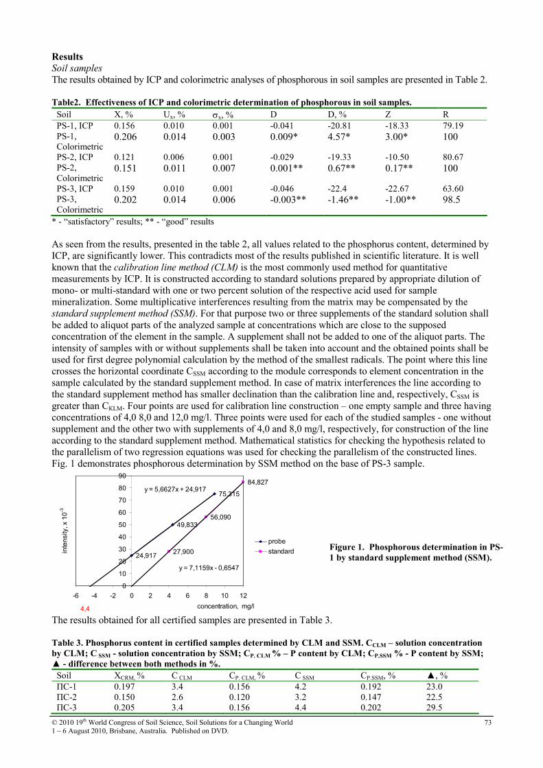
© 2010 19th World Congress of Soil Science, Soil Solutions for a Changing World
1 – 6 August 2010, Brisbane, Australia. Published on DVD. 73
Results Soil samples
The results obtained by ICP and colorimetric analyses of phosphorous in soil samples are presented in Table 2.
Table2. Effectiveness of ICP and colorimetric determination of phosphorous in soil samples.
Soil X, % Ux, % σx, % D D, % Z R
PS-1, ICP 0.156 0.010 0.001 -0.041 -20.81 -18.33 79.19
PS-1,
Colorimetric 0.206 0.014 0.003 0.009* 4.57* 3.00* 100
PS-2, ICP 0.121 0.006 0.001 -0.029 -19.33 -10.50 80.67
PS-2,
Colorimetric 0.151 0.011 0.007 0.001** 0.67** 0.17** 100
PS-3, ICP 0.159 0.010 0.001 -0.046 -22.4 -22.67 63.60
PS-3,
Colorimetric 0.202 0.014 0.006 -0.003** -1.46** -1.00** 98.5
* - “satisfactory” results; ** - “good” results
As seen from the results, presented in the table 2, all values related to the phosphorus content, determined by
ICP, are significantly lower. This contradicts most of the results published in scientific literature. It is well
known that the calibration line method (CLM) is the most commonly used method for quantitative
measurements by ICP. It is constructed according to standard solutions prepared by appropriate dilution of
mono- or multi-standard with one or two percent solution of the respective acid used for sample
mineralization. Some multiplicative interferences resulting from the matrix may be compensated by the
standard supplement method (SSM). For that purpose two or three supplements of the standard solution shall
be added to aliquot parts of the analyzed sample at concentrations which are close to the supposed
concentration of the element in the sample. A supplement shall not be added to one of the aliquot parts. The
intensity of samples with or without supplements shall be taken into account and the obtained points shall be
used for first degree polynomial calculation by the method of the smallest radicals. The point where this line
crosses the horizontal coordinate CSSM according to the module corresponds to element concentration in the
sample calculated by the standard supplement method. In case of matrix interferences the line according to
the standard supplement method has smaller declination than the calibration line and, respectively, CSSM is
greater than СКLM. Four points are used for calibration line construction – one empty sample and three having
concentrations of 4,0 8,0 and 12,0 mg/l. Three points were used for each of the studied samples - one without
supplement and the other two with supplements of 4,0 and 8,0 mg/l, respectively, for construction of the line
according to the standard supplement method. Mathematical statistics for checking the hypothesis related to
the parallelism of two regression equations was used for checking the parallelism of the constructed lines.
Fig. 1 demonstrates phosphorous determination by SSM method on the base of PS-3 sample.
24,917
49,833
75,315
27,900
56,090
84,827y = 5,6627x + 24,917
y = 7,1159x - 0,6547
0
10
20
30
40
50
60
70
80
90
-6 -4 -2 0 2 4 6 8 10 12
concentration, mg/l
inte
nsity, x 1
0 -3
probe
standard
4,4 The results obtained for all certified samples are presented in Table 3.
Table 3. Phosphorus content in certified samples determined by CLM and SSM. СCLM – solution concentration
by CLM; С SSM - solution concentration by SSM; СР. CLM % – P content by CLM; СР.SSM % - P content by SSM;
- difference between both methods in %.
Soil XCRM, % С CLM СР. CLM, % С SSM СР.SSM, % , %
ПС-1
ПС-2
ПС-3
0.197
0.150
0.205
3.4
2.6
3.4
0.156
0.120
0.156
4.2
3.2
4.4
0.192
0.147
0.202
23.0
22.5
29.5
Figure 1. Phosphorous determination in PS-
1 by standard supplement method (SSM).
© 2010 19th World Congress of Soil Science, Soil Solutions for a Changing World
1 – 6 August 2010, Brisbane, Australia. Published on DVD. 74
As seen from the data, presented in table 3 the phosphorus content determined by the standard supplement
method in the three samples significantly exceeds the phosphorus content determined by the calibration line
method, and the extraction degree is 100 % in all three cases. Although the matrix interference for all three
studied samples was close, the introduction of a common correction factor for the results obtained by the
calibration line method required accumulation of more experimental results and their mathematical
processing.
Plant materials
The results obtained for CTA-VTL-2 (Virginia tobacco leaves), digested by EPA method 3052 and dry
ashing are presented in Table 4.
Table 4. Effectiveness of ICP and colorimetric determination of phosphorous content in tobacco leaves. XCRM =
2204 ppm, σσσσCRM = 78 ppm.
Method X , ppm σx, ppm D D, % Z R
Dry ashing, ICP 2430 220 226* 10,25* 2,90* 100
Dry ashing,
colorimetric 2260 112 56** 2.54** 0.72** 100
EPA method 3052,
ICP 2355 110 151** 7.08** 2.00** 100
EPA method 3052,
colorimetric 2430 95 226* 10.25* 2.90* 100
* - “satisfactory” results; ** - “good” results
As seen from the data colorimetric and ICP methods for total phosphorus determination are highly correlated
and the results are generally within 5 to 10 % of each other.
Conclusion The results of the determination of total phosphorus in soils by ICP after complete sample dissolution by HF
showed that the calibration line method provided lower values. That is why simultaneous determination of P
with other macro- and microelements is risky. In all cases we have to use standard supplement method in
order to obtain correct results. In the case of plant materials phosphorous content can be determined directly
by the calibration line method.
Acknowledgement This work is supported by Bulgarian Ministry of Education, Project DO-02-87/08 and NSFB project GAMA
DO 02-70 11/12/2008
References Entwistle JA, Abrahams PW (1997) Multi-Element analysis of soils and sediments from scottish historical
sites. the potential of inductively coupled plasma-mass spectrometry for rapid site investigation. Journal
of Archaeological Science 24, 407-416.
ISO 14869-1(2001) Soil Quality. Dissolution for the Determination of Total Element Content, Part 1:
Dissolution with Hydrofluoric and Perchloric Acids.
Holliday VT, William GG (2007) Methods of soil P analysis in archaeology. Journal of Archaeological
Science 34, 301-333.
Mehlih A (1984) Mehlih 3 soil test extractant: A modification of Mehlih 2 extractant. Communications in
Soil Science and Plant Analysis 15(12), 1409-1416.
Pittman JJ, Zhang H, Schroder JL, Payton ME (2005) Differences of phosphorus in Mehlich3 extracts
determined by colorimetric and spectroscopic methods. Communications in Soil Science and Plant
Analysis 36, 1641-1659.
Pierzynski G, Zhang H, Wolf A, Kleinman PJ, Mallarino A, Sullivan D (2005) Phosphorus determination in
waters and extracts of soils and by-products: Inductively-coupled plasma spectrometry versus
colorimetric procedures. SERA-17 Policy Workgroup Paper [Online]. SERA-17. Available at
http://www.sera17.ext.vt.edu/Documents/P_Analysis_Comparisons.pdf (verified 20 Mar 2007).
Sikora FJ, Howe PS, Hill LE, Reid DC, Harover DE (2005) Comparison of colorimetric and ICP
determination of Phosphorus in Mehlich3 Soil extracts. Communications in Soil Science and Plant
Analysis 36, 875-887.
S Gorbanov, Velchev V, Matev J, Tanev Z, Rachovski G, Tomov T (1990) Handbook of agrochemistry, Sofia.
© 2010 19th World Congress of Soil Science, Soil Solutions for a Changing World
1 – 6 August 2010, Brisbane, Australia. Published on DVD. 75
In situ temporal and spatial monitoring of the structure of a compacted and
cultivated loamy soil by the 2D ERT method
Maud Ségera, Arlene Besson
a, Isabelle Cousin
a, Guillaume Giot
a, Julien Thiesson
a,b, Antonietta Agrillo
a,c,
Bernard Nicoullauda, Guy Richard
a
a INRA, UR0272 Science du Sol, Centre de Recherche d’Orléans, 2163 Avenue de la Pomme de Pin, CS 10001 Ardon, F-45075
Orléans cedex 2, France, Email [email protected] b UMR 7619 Sisyphe, Université Paris 6, 4 place Jussieu 75252 Paris cedex 5, Email [email protected] c Department of Soil, Plant, Environmental and Animal Production Sciences, University of Naples Federico II, Via Università 100,
80055, Portici (Na), Italy, Email [email protected]
Abstract Temporal and spatial monitoring of soil structural heterogeneity is useful to predict physical changes in soils.
Usual methods implemented to characterise soil structure are generally destructive and time-consuming.
Further technical solutions are then required to describe rapidly the soil structure without any disturbance.
Electrical resistivity tomography (ERT) was proven to be efficient technique for detecting accurately zones
with contrasted bulk density. Consequently space and time changes in soil structure might be characterized
by ERT. We aimed then at testing this possibility by using the 2D ERT method.
We have monitored for 8 months a typical Luvisol by ERT. The soil was initially and locally compacted by a
heavy tractor in the objective of creating zones of high bulk density. The studied plot encompassed bare soil
and wheat crop. ERT results indicated the soil drying process which occurred in summer and particularly
under wheat crop. We show also that electrical resistivity was higher in summer with local zone of very high
resistivity probably due to soil cracking.
Introduction Soil structure i.e. the arrangement of soil particles in space (Guérif 1987) is one of the factors controlling the
physical quality of soils. In agricultural context, soil structure changes in space and time as function of plants
growth, earthworm’s activity, tillage, and climate. Compaction related to in-field traffic can modify
significantly structure of cultivated layers in increasing bulk density. Soil compaction results in physical soil
degradations as well in agronomic and environmental problems. Solutions are then required to characterise
spatial and temporal changes in soil structure. Several methods were already developed to describe structural
components at the profile scale (i.e. at macrostructural scale). For instance, these last ones are based on the
visual description of a soil pit (Roger-Estrade et al. 2004), on soil sampling and measurements of soil
properties such as bulk density, porosity, water retention, and penetration resistance, or on characterisation of
the water infiltration. However these methods disturb soil and are also time-consuming. As a result, they
cannot be implemented (or otherwise hardly) for a spatial and temporal monitoring of the soil structural
heterogeneity.
Reversely electrical resistivity was proven to be a useful and efficient technique for soil structure description
(Besson et al. 2004; Séger et al. 2009) at scale of entire soil profile. Electrical resistivity of soils depends on
several soil parameters as, for instance, the volumetric clay and water contents, according to preferential
electrical pathways within pores filled in water and at the surface of clay particles. Consequently, electrical
resistivity should depend on soil bulk density and more generally on soil structural changes in space and
time.
We aim then at examining the efficiency of Electrical Resisitivity Tomography (ERT) technique for
characterising space and time changes of the soil structure within tilled layer of agricultural field, i.e.
changes in soil macrostructure due to traffic (compaction) and climate activity (crack formation). The studied
site presents a Luvisol (Beauce region, France).
This work corresponded to a section of the FP7-DIGISOIL project on “Integrated system of data collection
technologies for mapping soil properties”.
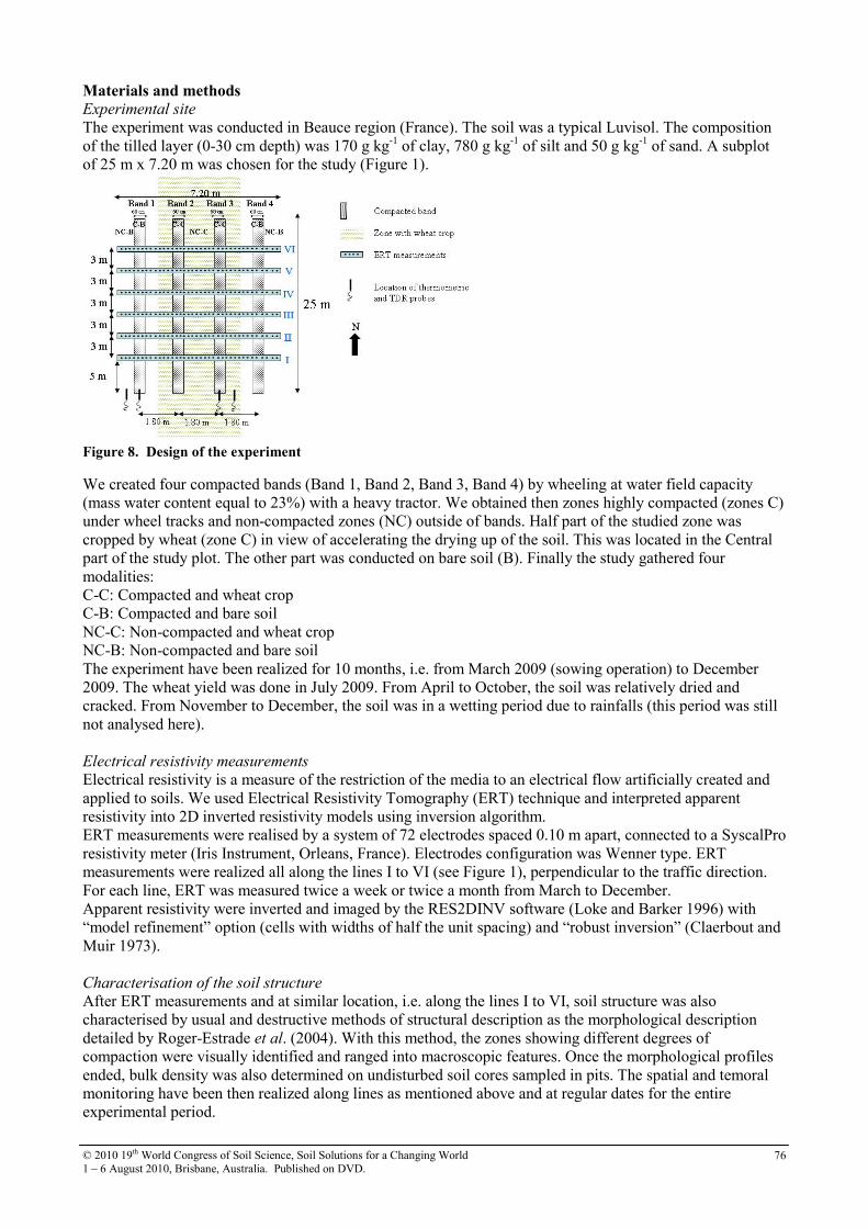
© 2010 19th World Congress of Soil Science, Soil Solutions for a Changing World
1 – 6 August 2010, Brisbane, Australia. Published on DVD. 76
Materials and methods Experimental site
The experiment was conducted in Beauce region (France). The soil was a typical Luvisol. The composition
of the tilled layer (0-30 cm depth) was 170 g kg-1
of clay, 780 g kg-1
of silt and 50 g kg-1
of sand. A subplot
of 25 m x 7.20 m was chosen for the study (Figure 1).
Figure 8. Design of the experiment
We created four compacted bands (Band 1, Band 2, Band 3, Band 4) by wheeling at water field capacity
(mass water content equal to 23%) with a heavy tractor. We obtained then zones highly compacted (zones C)
under wheel tracks and non-compacted zones (NC) outside of bands. Half part of the studied zone was
cropped by wheat (zone C) in view of accelerating the drying up of the soil. This was located in the Central
part of the study plot. The other part was conducted on bare soil (B). Finally the study gathered four
modalities:
C-C: Compacted and wheat crop
C-B: Compacted and bare soil
NC-C: Non-compacted and wheat crop
NC-B: Non-compacted and bare soil
The experiment have been realized for 10 months, i.e. from March 2009 (sowing operation) to December
2009. The wheat yield was done in July 2009. From April to October, the soil was relatively dried and
cracked. From November to December, the soil was in a wetting period due to rainfalls (this period was still
not analysed here).
Electrical resistivity measurements
Electrical resistivity is a measure of the restriction of the media to an electrical flow artificially created and
applied to soils. We used Electrical Resistivity Tomography (ERT) technique and interpreted apparent
resistivity into 2D inverted resistivity models using inversion algorithm.
ERT measurements were realised by a system of 72 electrodes spaced 0.10 m apart, connected to a SyscalPro
resistivity meter (Iris Instrument, Orleans, France). Electrodes configuration was Wenner type. ERT
measurements were realized all along the lines I to VI (see Figure 1), perpendicular to the traffic direction.
For each line, ERT was measured twice a week or twice a month from March to December.
Apparent resistivity were inverted and imaged by the RES2DINV software (Loke and Barker 1996) with
“model refinement” option (cells with widths of half the unit spacing) and “robust inversion” (Claerbout and
Muir 1973).
Characterisation of the soil structure
After ERT measurements and at similar location, i.e. along the lines I to VI, soil structure was also
characterised by usual and destructive methods of structural description as the morphological description
detailed by Roger-Estrade et al. (2004). With this method, the zones showing different degrees of
compaction were visually identified and ranged into macroscopic features. Once the morphological profiles
ended, bulk density was also determined on undisturbed soil cores sampled in pits. The spatial and temoral
monitoring have been then realized along lines as mentioned above and at regular dates for the entire
experimental period.
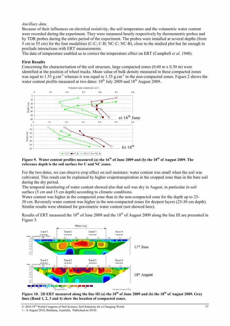
© 2010 19th World Congress of Soil Science, Soil Solutions for a Changing World
1 – 6 August 2010, Brisbane, Australia. Published on DVD. 77
Ancillary data
Because of their influences on electrical resistivity, the soil temperature and the volumetric water content
were recorded during the experiment. They were measured hourly respectively by thermometric probes and
by TDR probes during the entire period of the experiment. The probes were installed at several depths (from
5 cm to 55 cm) for the four modalities (C-C; C-B; NC-C; NC-B), close to the studied plot but far enough to
preclude interactions with ERT measurements.
The data of temperature enabled us to correct the temperature effect on ERT (Campbell et al. 1948).
First Results Concerning the characterisation of the soil structure, large compacted zones (0.60 m x 0.30 m) were
identified at the position of wheel tracks. Mean value of bulk density measured in these compacted zones
was equal to 1.55 g.cm-3
whereas it was equal to 1.35 g.cm-3
in the non-compacted zones. Figure 2 shows the
water content profile measured at two dates: 10th July 2009 and 18
th August 2009.
0
10
20
30
40
50
60
0 0.1 0.2 0.3 0.4 0.5 0.6
Volumetric water content (cm3.cm
-3)
Dep
th (
cm)
0
10
20
30
40
50
60
0 0.1 0.2 0.3 0.4 0.5 0.6
Dep
th (
cm)
C-C C-B NC-C NC-B
Figure 9. Water content profiles measured (a) the 16
th of June 2009 and (b) the 18
th of August 2009. The
reference depth is the soil surface for C and NC zones.
For the two dates, we can observe crop effect on soil moisture: water content was small when the soil was
cultivated. This result can be explained by higher evapotranspiration in the cropped zone than in the bare soil
during the dry period.
The temporal monitoring of water content showed also that soil was dry in August, in particular in soil
surface (5 cm and 15 cm depth) according to climatic conditions.
Water content was higher in the compacted zone than in the non-compacted zone for the depth up to 25-
30 cm. Reversely water content was higher in the non-compacted zones for deepest layers (25-30 cm depth).
Similar results were obtained for gravimetric water content (not showed here).
Results of ERT measured the 10th of June 2009 and the 18
th of August 2009 along the line III are presented in
Figure 3.
Figure 10. 2D ERT measured along the line III (a) the 10
th of June 2009 and (b) the 18
th of August 2009. Grey
lines (Band 1, 2, 3 and 4) show the location of compacted zones.
a) 16th
June
b) 18th

© 2010 19th World Congress of Soil Science, Soil Solutions for a Changing World
1 – 6 August 2010, Brisbane, Australia. Published on DVD. 78
We can identify compacted bands on ERT and in particular in near soil surface (from about 0 to 0.1 m depth.
Indeed resistivities were small with values close to 15 ohm.m.
Reversely, high values of resistivity increasing with time were encountered in the first 40 centimetres of soil
and in the central area of ERT (between 1.6 and 5.6 m). This zone corresponded to the cropped system which
was propably responsible for a huge drying of the soil.
To comfort ERT results as obtained in field conditions, we have realized additional laboratory experiments
which consisted in measuring electrical resistivity on soil cores at given bulk density and for a water content
range generally encountered in field. We aimed then at better describing the relationship between
geophysical data and soil variables of interest, i.e. the bulk density and soil water content, for such type of
soil. We could then observe, for instance, that electrical resistivity varied from 20 to 70 ohm.m when the
bulk density was equal to 1.45 g.cm-3
and when water content ranged from 10% to 22%. As a consequence,
the high values (up to 250 ohm.m) obtained in the central area of ERT (as shown on Figure 3b for the 18th of
August 2009), could not be explained only by drying. Another physical process could interact on resistivity,
i.e. soil cracking. Indeed cracks are filled in air. They represent then structural components electrically
resistant.
Conclusion This study aimed at monitoring soil structure in time and space in 2D by ERT technique. ERT results shows
that wheat crop is responsible for a huge drying of soil. Very high values of electrical resistivity measured in
August could be explained by soil cracking. This process cannot be detected by usual and destructive
methods. Electrical Resistivity Tomography appears then as a promising and useful tool for in-situ non-
destructive temporal monitoring of soil structure.
References Besson A, Cousin I, Samouëlian A, Boizard H, Richard G (2004) Structural heterogeneity of the soil tilled
layer as characterized by 2D electrical resistivity surveying. Soil & Tillage Research 79, 239-249.
Campbell RB, Bower CA, Richard LA (1948) Change in electrical conductivity with temperature and the
relation with osmotic pressure to electrical conductivity and ion concentration for soil extracts. Soil
Science Society of America Proceedings 13, 33–69.
Claerbout J, Muir F (1973) Robust modeling of erratic data. Geophysics 38, 826–844.
Guérif J (1987) L’analyse de la porosité : Application à l’étude du compactage des sols. Soil compaction and
regeneration CEC Worshop on soil compaction/ Avignon 17-18 Sept. 1985, (Eds. G Monnier, MJ
Goss), pp. 1-13. (A.A.BALKEMA/ROTTERDAM).
Loke MH, Barker RD (1996) Rapid least-squares inversion of apparent resistivity pseudosections by a quasi-
Newton method. Geophysical Prospecting 44, 131-152.
Roger-Estrade J, Richard G, Caneill J, Boizard H, Coquet Y, Defossez P, Manichon H (2004) Morphological
characterisation of soil structure in tilled fields: from a diagnosis method to the modelling of structural
changes over time. Soil & Tillage Research 79, 33-49.
Séger M, Cousin I, Frison A, Boizard H, Richard G (2009) Characterisation of the structural heterogeneity of
the soil tilled layer by using in situ 2D and 3D electrical resistivity measurements. Soil & Tillage
Research 103, 387-398.
© 2010 19th World Congress of Soil Science, Soil Solutions for a Changing World
1 – 6 August 2010, Brisbane, Australia. Published on DVD. 79
IR assessment of C in tropical soils
Beata E. MadariA, James B. Reeves III
B, Diego M. Souza
A, Pedro L. O. A. Machado
A and Vinicius M.
BenitesC
AEmbrapa Rice and Beans, Santo Antônio de Goiás, GO, Brazil, Email [email protected], [email protected],
[email protected] BEMBUL, HRSL, ANRI, ARS, USDA, USA, Email [email protected] CEmbrapa Soils, Rio de Janeiro, RJ, Brazil, Email [email protected]
Abstract Calibrations for soil carbon content measured by dry combustion (Total Carbon, TC) and chromate oxidation
(Organic Carbon, CORG) of soils from the Brazilian National Soil Collection were made using Fourier
Transform Near- and Mid-Infrared Diffuse Reflectance Spectroscopy combined with PLS statistics.
Calibration sets of sample populations of different carbon ranges, soil taxonomic classes, and soil textural
groups were established. Calibrations obtained for the largest TC and CORG ranges were better, compared to
the lower ones, but lower RMSD and RD were found for the lower carbon ranges. Taxonomic soil class was
not an adequate criterion for calibration set formation. Soil texture had effects on calibrations, especially
using NIRS, because of the particular size effect to which NIRS was more sensitive than Mid-IR. In general,
DRIFTS showed better performance than NIRS. NIRS only outperformed DRIFTS when used with a
calibration set that was fairly homogeneous in its particle size distribution. Results demonstrated that while
calibrations can be developed using either DRIFTS or NIRS for even a very diverse set of soil samples,
which will determine C over a wide range of concentrations inherent in such a diverse set, it is desirable to
separate sample populations by soil textural properties for calibration development to achieve more accurate
results.
Key Words Chemometrics, granulometric composition, bulk soil
Introduction The application of infrared spectroscopy (near- and mid-IR) for the quantitative analysis of soils has become
of increased interest over the last one and a half decades or so. One of the main reasons is the need for new
methodologies for the assessment of C forms in soils and the potential of the technique both for laboratory
and field measurements. Potential future policies for C sequestration in agriculture (crop production systems
and pasture grazing) and forestry (particularly eucalyptus and pine plantations) would require the
measurement of soil C over time at many locations to evaluate how much C is being sequestered or lost from
the soil. Standard methods such as chromate oxidation or high temperature combustion are slow, expensive
or both. Loss-on-ignition, which is a fairly cheap and fast method, for highly weathered tropical soils suffers
from accuracy problems (Nelson and Sommers 1996; Watson et al. 2000; Lal et al. 2001).
Infrared spectroscopy, in turn, is a technique that is able to measure large number of samples, and determine
any number of analytes at a time, once calibrations are developed (Reeves et al. 1999). There is numerous
literature about the types of soil parameters, such as total C (CTOT), organic C (CORG), forms of N,
macroelements, texture etc., that can be potentially determined by IR spectroscopy (e.g. Viscarra-Rossel et
al. 2006).
For application on soils, mid-IR Fourier-transform diffuse reflectance spectroscopy (DRIFTS) seems to be
more robust than near infrared (NIRS) (Madari et al. 2005), however, the application of either of them is not
always straightforward for the several possible levels of future application. Fairly accurate calibrations can
be developed for the local level (e.g. plot or even farm) (Madari et al. 2006), but to achieve robust
calibrations at regional or national level criteria for calibration development has to be investigated.
The objective of this study was to investigate what kind of major criteria could be applied when sample
populations for calibration development are to be selected, in the case of soils, to determine TC and CORG
with the highest accuracy possible using around 1000 samples from the National Soil Collection of the
Brazilian Agricultural Research Corporation (Embrapa) complemented by some Ferralsol samples from the
collection of the Institute of Agronomy (IAC-Campinas, São Paulo State of Brazil).
Methods Samples
Three hundred and sixty seven soil profiles from all Brazilian biomes were selected from the National Soil
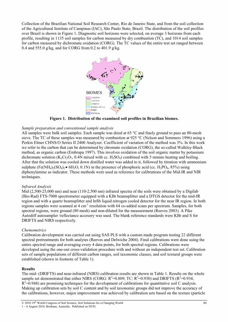
© 2010 19th World Congress of Soil Science, Soil Solutions for a Changing World
1 – 6 August 2010, Brisbane, Australia. Published on DVD. 80
Collection of the Brazilian National Soil Research Center, Rio de Janeiro State, and from the soil collection
of the Agricultural Institute of Campinas (IAC), São Paulo State, Brazil. The distribution of the soil profiles
over Brazil is shown in Figure 1. Diagnostic soil horizons were selected, on average 3 horizons from each
profile, resulting in 1135 soil samples for carbon measured by dry combustion (TC), and 1014 soil samples
for carbon measured by dichromate oxidation (CORG). The TC values of the entire test set ranged between
0.4 and 555.0 g/kg, and for CORG from 0.2 to 401.9 g/kg.
BIOMES
Figure 1. Distribution of the examined soil profiles in Brazilian biomes.
Sample preparation and conventional sample analysis
All samples were bulk soil samples. Each sample was dried at 65 °C and finely ground to pass an 80-mesh
sieve. The TC of these samples was measured by combustion at 925 °C (Nelson and Sommers 1996) using a
Perkin Elmer CHNS/O Series II 2400 Analyzer. Coefficient of variation of the method was 3%. In this work
we refer to the carbon that can be determined by chromate oxidation (CORG), the so-called Walkley-Black
method, as organic carbon (Embrapa 1997). This involves oxidation of the soil organic matter by potassium
dichromate solution (K2Cr2O7, 0.4N mixed with cc. H2SO4) combined with 5 minute heating and boiling.
After that the solution was cooled down distilled water was added to it, followed by titration with ammonium
sulphate (Fe(NH4)2(SO4)2 • 6H2O, 0.1N) in the presence of phosphoric acid (cc. H3PO4, 85%) using
diphenylamine as indicator. These methods were used as reference for calibrations of the Mid-IR and NIR
techniques.
Infrared Analysis
Mid (2,500-25,000 nm) and near (110-2,500 nm) infrared spectra of the soils were obtained by a Digilab
(Bio-Rad) FTS-7000 spectrometer equipped with a KBr beamsplitter and a DTGS detector for the mid-IR
region and with a quartz beamsplitter and InSb liquid nitrogen cooled detector for the near IR region. In both
regions samples were scanned at 4 cm-1
resolution with 64 co-added scans per spectrum. Samples, for both
spectral regions, were ground (80 mesh) and non-diluted for the measurement (Reeves 2003). A Pike
Autodiff autosampler /reflectance accesory was used. The blank reference standards were KBr and S for
DRIFTS and NIRS respectively.
Chemometrics
Calibration development was carried out using SAS PLS with a custom made program testing 22 different
spectral pretreatments for both analytes (Reeves and Delwiche 2004). Final calibrations were done using the
entire spectral range and averaging every 4 data points, for both spectral regions. Calibrations were
developed using the one-out cross-validation procedure with and without an independent test set. Calibration
sets of sample populations of different carbon ranges, soil taxonomic classes, and soil textural groups were
established (shown in footnote of Table 1).
Results The mid- (DRIFTS) and near-infrared (NIRS) calibration results are shown in Table 1. Results on the whole
sample set demonstrated that either NIRS (CORG: R2=0.809; TC: R
2=0.930) and DRIFTS (R
2=0.934;
R2=0.948) are promising techniques for the development of calibrations for quantitative soil C analysis.
Making up calibration sets by soil C content and by soil taxonomic groups did not improve the accuracy of
the calibrations, however, major improvement was achieved by calibration sets based on the texture (particle
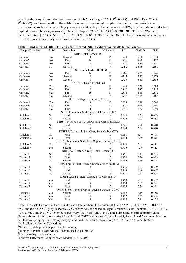
© 2010 19th World Congress of Soil Science, Soil Solutions for a Changing World
1 – 6 August 2010, Brisbane, Australia. Published on DVD. 81
size distribution) of the individual samples. Both NIRS (e.g. CORG: R2=0.975) and DRIFTS (CORG:
R2=0.967) performed well on the calibration set that contained samples that had similar particle size
distributions, such as the very clayey samples (>60% clay). The accuracy of NIRS, however, decreased when
applied to more heterogeneous sample sets (clayey [CORG: NIRS R2=0.938, DRIFTS R
2=0.962] and
medium texture [CORG: NIRS R2=0.871, DRIFTS R
2=0.917]), while DRIFTS kept showing good accuracy.
The difference in accuracy was more evident for CORG.
Table 1. Mid-infrared (DRIFTS) and near infrared (NIRS) calibration results for soil carbon.
1Sample Data Sets 2MSC Derivative 3GAP 4# Factors R2 5RMSD 6RD
NIRS, Total Carbon (TC)
Carbon1 No Second 8 15 0.931 17.66 0.574
Carbon2 No First 16 13 0.739 7.90 0.473
Carbon 3 No First 8 12 0.750 4.80 0.356
Carbon 4 No Second 4 4 0.952 34.56 0.180
NIRS, Organic Carbon (CORG)
Carbon 5 No First 16 13 0.809 18.55 0.968
Carbon 6 No Second 8 10 0712 5.23 0.478
Carbon 7 No Second 8 9 0.726 3.43 0.385
DRIFTS, Total Carbon (TC)
Carbon 1 Yes First 4 13 0.947 15.38 0.504
Carbon 2 Yes First 8 12 0.856 5.87 0.352
Carbon 3 Yes First 16 11 0.811 4.18 0.312
Carbon 4 No Second 4 4 0.948 36.14 0.188
DRIFTS, Organic Carbon (CORG)
Carbon 5 Yes First 8 13 0.934 10.88 0.568
Carbon 6 Yes First 4 12 0.810 4.24 0.400
Carbon 7 No First 6 11 0.840 2.62 0.294
NIRS, Taxonomic Soil Class, Total Carbon (TC)
Soilclass1 No First 16 9 0.725 7.65 0.433
Soilclass 2 No Second 4 5 0.854 5.72 0.383
NIRS, Taxonomic Soil Class, Organic Carbon (CORG)
Soilclass 3 No First 16 9 0.725 7.70 0.440
Soilclass 2 No Second 4 4 0.784 6.75 0.470
DRIFTS, Taxonomic Soil Class, Total Carbon (TC)
Soilclass 1 No First 4 10 0.861 5.44 0.308
Soilclass 2 Yes First 8 11 0.914 4.40 0.295
DRIFTS, Taxonomic Soil Class, Organic Carbon (CORG)
Soilclass 3 No First 4 10 0.862 5.45 0.312
Soilclass 4 Yes Second 16 10 0.905 4.49 0.313
NIRS, Soil Textural Group, Total Carbon (TC)
Texture1 No First 8 10 0.961 6.42 0.293
Texture 2 No First 8 12 0.930 7.26 0.359
Texture 3 No Second 32 8 0.866 6.39 0.345
NIRS, Soil Textural Group, Organic Carbon (CORG)
Texture 4 No Second 4 8 0.975 5.33 0.309
Texture 5 No First 8 12 0.938 7.00 0.487
Texture 6 No Second 32 8 0.871 6.37 0.568
DRIFTS, Soil Textural Group, Total Carbon (TC)
Texture1 Yes First 16 5 0.953 7.05 0.322
Texture 2 Yes First 4 12 0.954 5.89 0.291
Texture 3 Yes First 8 12 0.905 5.39 0.291
DRIFTS, Soil Textural Group, Organic Carbon (CORG)
Texture 4 Yes Second 32 7 0.967 6.19 0.358
Texture 5 Yes First 4 12 0.962 5.52 0.384
Texture 6 Yes First 8 13 0.917 5.11 0.455
1Calibration sets Carbon1 to 4 are based on soil total carbon (TC) content (0.4 ≤ C ≤ 555.0, 0.4 ≤ C ≤ 99.1, 0.4 ≤ C
39.9, and 0.8 ≤ C 555.0 g/kg, respectively); Carbon5 to 7 are based on organic carbon (CORG)content (0.2 ≤ C ≤ 401.9,
0.2 ≤ C 66.0, and 0.2 ≤ C 30.0 g/kg, respectively); Soilclass1 and 3 and 2 and 4 are based on soil taxonomy class
(Ferralsols and Acrisols, respectively) for TC and CORG calibration; Texture1 and 4, 2 and 5, and 3 and 6 are based on
soil textural grouping (very clayey, clayey, and medium texture, respectively) for TC and CORG calibration. 2Multiplicative Scatter Correction;
3Number of data points skipped for derivatives;
4Number of Partial Least Squares Factors used in calibration;
5Rootmean Squared Deviation;
6Relative Difference. Adapted from Madari et al. (2005).

© 2010 19th World Congress of Soil Science, Soil Solutions for a Changing World
1 – 6 August 2010, Brisbane, Australia. Published on DVD. 82
Conclusions Calibrations can be developed using either DRIFTS or NIRS for even a very diverse set of soil samples,
which will determine C over a wide range of concentrations inherent in such a diverse set. However, to
obtain more reliable predictions for soil C content using a very diverse set as calibration set does not appear
to be the most useful approach. Developing calibrations for ranges of soil C content decreased the error of
the calibrations (RMSD and RD), however, resulted in lower accuracy (R2). Calibrations based on soil
textural classes also do not seem to be the right approach for soil carbon content prediction. The reason for
this might be that calibrations using a set of samples of large variance in textural composition suffer from the
sensitivity of infrared spectroscopy on particle size distribution of the samples, especially in the case of
NIRS. Near infrared spectroscopy (NIRS) had excellent performance (R2 = 0.961-0.975) when applied for a
calibration set that contained samples that had very similar particle size distribution, but its performance
declined for more heterogeneous sample populations regarding particle size. Diffuse reflectance infrared
spectroscopy (DRIFTS), by being less influenced by specular effects, showed reasonable performance (R2 >
0.95) for sample sets containing soils of a wide range of particle size distribution. For calibration purposes
for soil carbon content (both TC and CORG) prediction, therefore, it seems to be desirable to create
calibration sets based on soil textural properties and then to use the most adequate spectral region (NIR for
the more homogeneous sets, or Mid-IR for the less homogeneous ones) for the calibration.
References Embrapa-Centro Nacional de Pesquisa de Solos (1997) Manual de métodos de análise de solo, 2nd Ed.pp.
47-49. (Centro Nacional de Pesquisa de Solos: Rio de Janeiro, Brazil).
Lal R., Kimble JM, Follett RF, Stewart BS (2001) Methods of assessment of soil carbon. (CRC Press: Boca
Raton, FL).
Madari BE, Reeves JB III, Coelho MR, Machado PLOA, De-Polli H, Coelho RM, Benites VM, Souza LF,
McCarty GW (2005) Mid- and Near-infrared Spectroscopic Determination of Carbon in a Diverse Set of
Soils from the Brazilian National Soil Collection. Spectroscopy Letters 38, 721–740.
Madari BE, Reeves JB III, Coelho MR, Machado PLOA, Torres E, Guimarães CM, McCarty GW (2006)
Mid- and near-infrared spectroscopic assessment of soil compositional parameters and structural indices
in two Ferralsols. Geoderma 136, 245-259.
Nelson DW, Sommers LE (1996) Total carbon, organic carbon, and organic matter. In ‘Methods of Soil
Analysis Part 3’ (Ed. D.L. Sparks, A.L. Page, P.A. Helmike, R.H. Loeppert, P.N. Softanpour, P.N. M.A.
Tabatabai, C.T. Johnston, M.E. Summer) Part 3, pp. 997-983. (SSSA-ASA: Madison, WI).
Reeves JB III (2003) Mid-infrared diffuse reflectance spectroscopy: Is sample dilution with KBr neccesary,
and if so, when. American Laboratory 35 (8), 24-28.
Reeves JB III, Delwiche SR (2004) Using SAS for PLS calibrations of spectroscopic data. NIRS News 15
(3), 10-15.
Reeves JB III, McCarty GV, Meisenger JJ (1999) Near infrared reflectance spectroscopy for the analysis of
agricultural soils. J. Near Infrared Spectroscopy 7, 179-193.
Viscarra Rossel RA, Walvoort TDJJ, McBratney AB, Janik LJ, Skjemstad JO (2006) Visible, near infrared,
mid infrared or combined diffuse reflectance spectroscopy for simultaneous assessment of various soil
properties. Geoderma 131, 59–75.
Watson RT, Noble IR, Bolin B, Ravindranath NH, Verardo DJ, Dokken DJ (2000) Land Use, Land-Use
Change, and Forestry, A Special Report of the IPCC, pp. 53-126. (Cambridge University Press:
Cambridge).

© 2010 19th World Congress of Soil Science, Soil Solutions for a Changing World
1 – 6 August 2010, Brisbane, Australia. Published on DVD. 83
iSOIL and Standardisation
Peter Dietrich, Uta Sauer and Ulrike Werban
Department Monitoring and Exploration Technologies, Helmholtz Centre for Environmental Research - UFZ, , Permoserstrasse 15,
04318 Leipzig, Germany, [email protected]
Abstract The project iSOIL “Interactions between soil related sciences – Linking geophysics, soil science and digital
soil mapping”. iSOIL focuses on improving and developing fast and reliable mapping approaches of soil
properties, soil functions, and soil degradation threats. This requires the improvement and integration of
advanced soil sampling approaches, geophysical and spectroscopic measurement techniques, as well as
pedometric and pedophysical approaches. A prerequisite for the application of geophysical measurements for
proximal soil sensing are reproducible and reliable data. The procedure of the CEN Workshop of the
European Committee for Standardization (CEN) seems to be an adequate framework to introduce
standardised procedures into geophysical measurements. Because electromagnetic induction measurements
(EMI) are widely used for soil mapping the existence of several problems with the comparability of EMI
results, we want to establish a widely accepted voluntary standard for a best practice of EMI with help of the
CEN Workshop.
Key Words Geophysics, Digital Soil Mapping, Pedophysics, CEN, Standardisation, electromagnetic induction method.
Introduction All terrestrial environmental processes involve the pedon, including hydrological, geological,
meteorological, ecological and anthropological. These processes occur in particular at the upper soil which is
the dynamic area from the land surface to the ground of the upper aquifer. Consequently investigations of
soil properties become an increasing importance for the majority of land and water resource management.
Fast and cost-effective techniques as well as recommendations for high resolution, economically feasible,
and target oriented soil mapping under conditions realistic for end-users are needed. The development and
evaluation of such techniques and recommendation is the aim of the iSOIL project. A general overview
about the project iSOIL will be given in the following. The reproducibility of data of a single geophysical
measurement method is the prerequisite for common interpretation of different methods. In our project we
focus on one geophysical method – the electromagnetic induction measurements for the proximal soil
sensing. We will give more details on one activity of the iSOIL project: the CEN Workshop” Best Practice
Approach for electromagnetic induction measurements of the near surface” to establish widely accepted
voluntary standard for a best practice of EMI measurement. Please see also our other presentation
“Acquisition and reliability of geophysical data in soil science” about results concerning reproducibility of
EM38DD data to show the importance and the need for such best practice approaches.
Project iSOIL iSOIL - “Interactions between soil related sciences – Linking geophysics, soil science and digital soil
mapping” is a project financed by the European Commission within the 7th Framework Program. The iSOIL
consortium consists of 19 partners from nine countries. In the project are involved universities, research
organizations as well as small and medium sized enterprises (see www.isoil.info).
The focus of the project iSOIL is to develop new and to improve existing strategies and innovative methods
for generating accurate, high-resolution soil property maps. At the same time the developments will reduce
costs compared to traditional soil mapping. The project tackles this challenge by integrating the following
three major components:
(i) high resolution, non-destructive geophysical (e.g. electromagnetic induction -EMI;
ground penetrating radar, magnetics, seismics), spectroscopic methods and other suitable
methods,
(ii) spatial inter- and extrapolations (e.g. geostatistics, machine learning) concepts
(McBratney et al. 2003), and
(iii) soil sampling and validation schemes to provide representative and transferable results
(Brus et al. 2006; de Gruiter et al. 2009; Behrens et al. 2009).
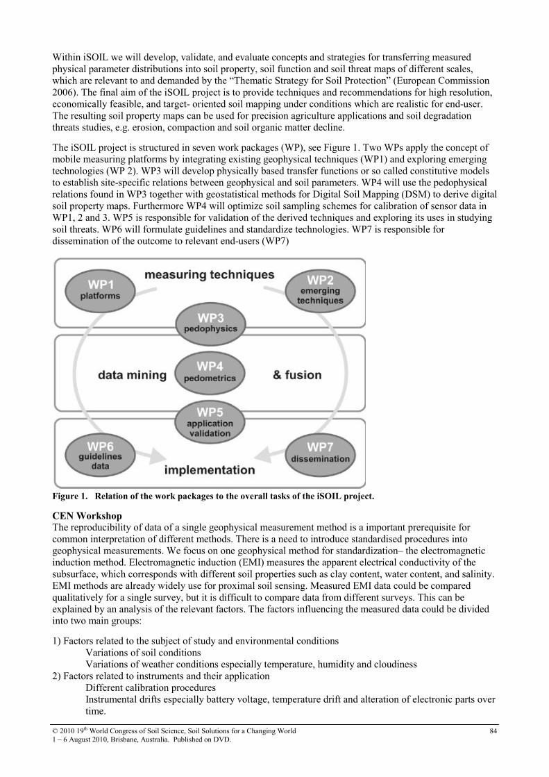
© 2010 19th World Congress of Soil Science, Soil Solutions for a Changing World
1 – 6 August 2010, Brisbane, Australia. Published on DVD. 84
Within iSOIL we will develop, validate, and evaluate concepts and strategies for transferring measured
physical parameter distributions into soil property, soil function and soil threat maps of different scales,
which are relevant to and demanded by the “Thematic Strategy for Soil Protection” (European Commission
2006). The final aim of the iSOIL project is to provide techniques and recommendations for high resolution,
economically feasible, and target- oriented soil mapping under conditions which are realistic for end-user.
The resulting soil property maps can be used for precision agriculture applications and soil degradation
threats studies, e.g. erosion, compaction and soil organic matter decline.
The iSOIL project is structured in seven work packages (WP), see Figure 1. Two WPs apply the concept of
mobile measuring platforms by integrating existing geophysical techniques (WP1) and exploring emerging
technologies (WP 2). WP3 will develop physically based transfer functions or so called constitutive models
to establish site-specific relations between geophysical and soil parameters. WP4 will use the pedophysical
relations found in WP3 together with geostatistical methods for Digital Soil Mapping (DSM) to derive digital
soil property maps. Furthermore WP4 will optimize soil sampling schemes for calibration of sensor data in
WP1, 2 and 3. WP5 is responsible for validation of the derived techniques and exploring its uses in studying
soil threats. WP6 will formulate guidelines and standardize technologies. WP7 is responsible for
dissemination of the outcome to relevant end-users (WP7)
Figure 1. Relation of the work packages to the overall tasks of the iSOIL project.
CEN Workshop The reproducibility of data of a single geophysical measurement method is a important prerequisite for
common interpretation of different methods. There is a need to introduce standardised procedures into
geophysical measurements. We focus on one geophysical method for standardization– the electromagnetic
induction method. Electromagnetic induction (EMI) measures the apparent electrical conductivity of the
subsurface, which corresponds with different soil properties such as clay content, water content, and salinity.
EMI methods are already widely use for proximal soil sensing. Measured EMI data could be compared
qualitatively for a single survey, but it is difficult to compare data from different surveys. This can be
explained by an analysis of the relevant factors. The factors influencing the measured data could be divided
into two main groups:
1) Factors related to the subject of study and environmental conditions
Variations of soil conditions
Variations of weather conditions especially temperature, humidity and cloudiness
2) Factors related to instruments and their application
Different calibration procedures
Instrumental drifts especially battery voltage, temperature drift and alteration of electronic parts over
time.
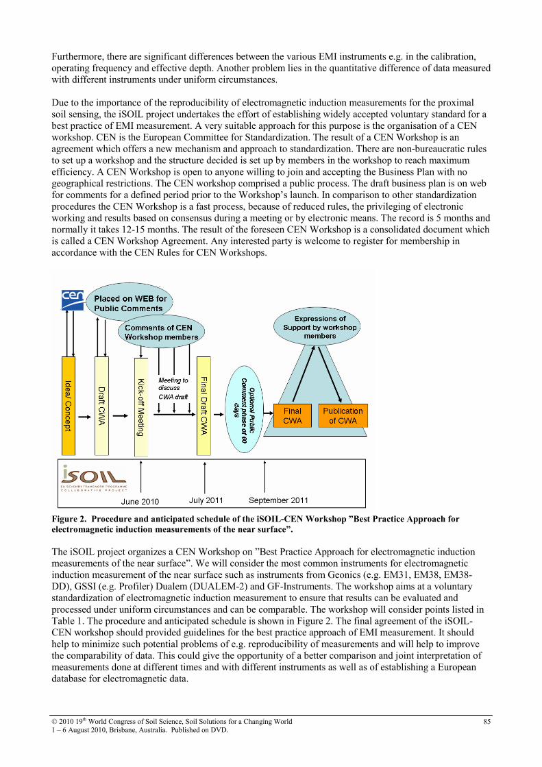
© 2010 19th World Congress of Soil Science, Soil Solutions for a Changing World
1 – 6 August 2010, Brisbane, Australia. Published on DVD. 85
Furthermore, there are significant differences between the various EMI instruments e.g. in the calibration,
operating frequency and effective depth. Another problem lies in the quantitative difference of data measured
with different instruments under uniform circumstances.
Due to the importance of the reproducibility of electromagnetic induction measurements for the proximal
soil sensing, the iSOIL project undertakes the effort of establishing widely accepted voluntary standard for a
best practice of EMI measurement. A very suitable approach for this purpose is the organisation of a CEN
workshop. CEN is the European Committee for Standardization. The result of a CEN Workshop is an
agreement which offers a new mechanism and approach to standardization. There are non-bureaucratic rules
to set up a workshop and the structure decided is set up by members in the workshop to reach maximum
efficiency. A CEN Workshop is open to anyone willing to join and accepting the Business Plan with no
geographical restrictions. The CEN workshop comprised a public process. The draft business plan is on web
for comments for a defined period prior to the Workshop’s launch. In comparison to other standardization
procedures the CEN Workshop is a fast process, because of reduced rules, the privileging of electronic
working and results based on consensus during a meeting or by electronic means. The record is 5 months and
normally it takes 12-15 months. The result of the foreseen CEN Workshop is a consolidated document which
is called a CEN Workshop Agreement. Any interested party is welcome to register for membership in
accordance with the CEN Rules for CEN Workshops.
Figure 2. Procedure and anticipated schedule of the iSOIL-CEN Workshop ”Best Practice Approach for
electromagnetic induction measurements of the near surface”.
The iSOIL project organizes a CEN Workshop on ”Best Practice Approach for electromagnetic induction
measurements of the near surface”. We will consider the most common instruments for electromagnetic
induction measurement of the near surface such as instruments from Geonics (e.g. EM31, EM38, EM38-
DD), GSSI (e.g. Profiler) Dualem (DUALEM-2) and GF-Instruments. The workshop aims at a voluntary
standardization of electromagnetic induction measurement to ensure that results can be evaluated and
processed under uniform circumstances and can be comparable. The workshop will consider points listed in
Table 1. The procedure and anticipated schedule is shown in Figure 2. The final agreement of the iSOIL-
CEN workshop should provided guidelines for the best practice approach of EMI measurement. It should
help to minimize such potential problems of e.g. reproducibility of measurements and will help to improve
the comparability of data. This could give the opportunity of a better comparison and joint interpretation of
measurements done at different times and with different instruments as well as of establishing a European
database for electromagnetic data.
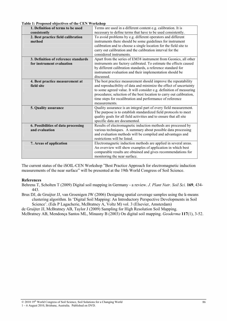
© 2010 19th World Congress of Soil Science, Soil Solutions for a Changing World
1 – 6 August 2010, Brisbane, Australia. Published on DVD. 86
Table 1: Proposed objectives of the CEN Workshop
1. Definition of terms to be used
consistently
Terms are used in a different content e.g. calibration. It is
necessary to define terms that have to be used consistently.
2. Best practice field calibration
method
To avoid problems by e.g. different operators and different
instruments there should be some guidelines for instrument
calibration and to choose a single location for the field site to
carry out calibration and the calibration interval for the
considered instruments.
3. Definition of reference standards
for instrument evaluation
Apart from the series of EM38 instrument from Geonics, all other
instruments are factory calibrated. To estimate the effects caused
by different calibration standards, a reference standard for
instrument evaluation and their implementation should be
discussed.
4. Best practice measurement at
field site
The best practice measurement should improve the repeatability
and reproducibility of data and minimize the effect of uncertainty
to some agreed value. It will consider e.g. definition of measuring
procedures; selection of the best location to carry out calibration,
time steps for recalibration and performance of reference
measurements.
5. Quality assurance
Quality assurance is an integral part of every field measurement.
The purpose is to establish standardized field protocols to meet
quality goals for all field activities and to ensure that all site
specific data are documented.
6. Possibilities of data processing
and evaluation
Results of electromagnetic induction methods are processed by
various techniques. A summary about possible data processing
and evaluation methods will be compiled and advantages and
restrictions will be listed.
7. Areas of application
Electromagnetic induction methods are applied in several areas.
An overview will show examples of application in which best
comparable results are obtained and gives recommendations for
monitoring the near surface.
The current status of the iSOIL-CEN Workshop ”Best Practice Approach for electromagnetic induction
measurements of the near surface” will be presented at the 19th World Congress of Soil Science.
References Behrens T, Scholten T (2009) Digital soil mapping in Germany - a review. J. Plant Nutr. Soil Sci. 169, 434-
443.
Brus DJ, de Gruijter JJ, van Groenigen JW (2006) Designing spatial coverage samples using the k-means
clustering algorithm. In ‘Digital Soil Mapping: An Introductory Perspective Developments in Soil
Science’. (Eds P Lagacherie, McBratney A, Voltz M) vol. 3 (Elsevier, Amsterdam)
de Gruijter JJ, McBratney AB, Taylor J (2009) Sampling for High Resolution Soil Mapping.
McBratney AB, Mendonça Santos ML, Minasny B (2003) On digital soil mapping. Geoderma 117(1), 3-52.
© 2010 19th World Congress of Soil Science, Soil Solutions for a Changing World
1 – 6 August 2010, Brisbane, Australia. Published on DVD. 87
Locating Soil Monitoring Sites Using Spatial Analysis of Multilayer Data
Viacheslav I. AdamchukA, Luan Pan
A, David B. Marx
B, and Derrel L. Martin
A
A Department of Biological Systems Engineering, University of Nebraska-Lincoln, Lincoln, Nebraska, USA. B Department of Statistics, University of Nebraska-Lincoln, Lincoln, Nebraska, USA.
E-mail: [email protected]
Abstract Wireless technology is increasingly used to monitor temporal changes in soil conditions. Because of the
limited number of such monitoring units that can be economically installed throughout an agricultural field,
it is critical to identify proper locations for these units. On-the-go soil sensing technology provides the
opportunity to rapidly obtain high-resolution data on soil spatial variability at a relatively low cost.
Prescribing representative monitoring sites based on multiple sensor-based data layers is an important
process, yet in practice, this selection is conducted in a very subjective manner. This research provides an
analytical methodology for assessing the quality of selection of a set of strategic locations in an agricultural
field. The methodology is shown using a combination of apparent soil electrical conductivity (ECa) and field
elevation maps to identify sites for water content monitoring.
Key Words On-the-go soil sensing, targeted sampling, electrical conductivity, elevation, irrigation.
Introduction The efficiency of a centre pivot irrigation system depends on its ability to meet the water demands of the
growing crop (Sadler et al. 2005). While limited water supplies can reduce crop yield due to water stress,
excessive irrigation can result in wasted resources and, if extreme, may also reduce yields. The optimum
quantity of irrigation water changes temporally and spatially. Various methods have been used to focus on
either level of variability. Thus, soil water monitoring and crop modelling often facilitate improved irrigation
scheduling. On the other hand, dense-resolution proximal soil sensing allows a producer to identify the
spatial variability of topsoil water storage capacity, which also affects the need for irrigation water. A
combination of data layers with high spatial resolution can be used to define targeted field locations for soil
water monitoring. The most appropriate strategy might be placement of a few sets of soil water sensors with
wireless communication capability in these locations. Since water storage capacity depends on the properties
of the soil profile and the potential for surface water runoff, high density measurement of apparent soil
electrical conductivity (ECa) and field elevation can be used to define field locations with different levels of
water available to the crop during the growing season.
Selecting the appropriate number of strategic locations within a field is critical, but this process is typically
subjective. Practitioners who use high-resolution data layers rely on the following general rules: 1) selected
locations must cover the entire range of data from each source; 2) selected locations must avoid field
boundaries and other transition zones; and 3) practitioners must spread locations over the entire field. While
these “guidelines” are useful, they do not translate into an operational algorithm and, therefore, can produce
numerous solutions that result in differing degrees of satisfaction. In principle, this process is similar to
prescribing the targeted sampling locations needed to calibrate high-resolution data or to quantify the
agronomic soil attributes of established management zones (Lesch 2005; Minasny and McBratney 2006;
Brus and Heuvelink 2007; de Gruijter et al. 2008). The objective of this paper is to define a set of criteria
that can be used to compare alternative schemes of soil sensor telemetry placement, basing these criteria on
the three general rules used to analyze soil ECa and field elevation maps.
Methods Optimization Criteria
As previously mentioned, the definition of the optimum guided sampling scheme is quite vague. There are
many parameters that can quantify 1) the spatial separation; 2) the spread across both sets of measurements;
and 3) the local homogeneity within each set of measurements. Furthermore, there are several alternatives to
deriving the overall objective function as a combination of these parameters. The goodness of spatial
separation among selected sampling locations can be assessed by comparing the field areas represented by
each sample; by comparing the variance of the error for an interpolated surface; or by calculating the
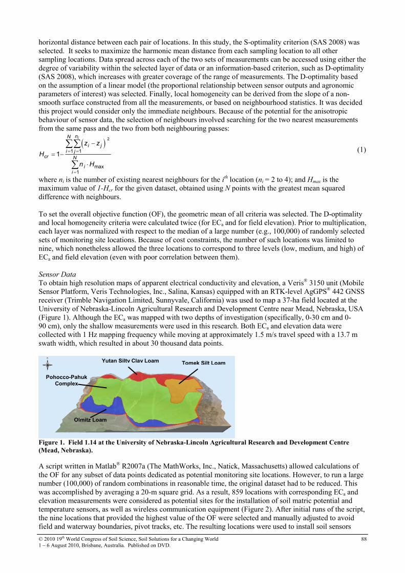
© 2010 19th World Congress of Soil Science, Soil Solutions for a Changing World
1 – 6 August 2010, Brisbane, Australia. Published on DVD. 88
horizontal distance between each pair of locations. In this study, the S-optimality criterion (SAS 2008) was
selected. It seeks to maximize the harmonic mean distance from each sampling location to all other
sampling locations. Data spread across each of the two sets of measurements can be accessed using either the
degree of variability within the selected layer of data or an information-based criterion, such as D-optimality
(SAS 2008), which increases with greater coverage of the range of measurements. The D-optimality based
on the assumption of a linear model (the proportional relationship between sensor outputs and agronomic
parameters of interest) was selected. Finally, local homogeneity can be derived from the slope of a non-
smooth surface constructed from all the measurements, or based on neighbourhood statistics. It was decided
this project would consider only the immediate neighbours. Because of the potential for the anisotropic
behaviour of sensor data, the selection of neighbours involved searching for the two nearest measurements
from the same pass and the two from both neighbouring passes:
( )inN
i ji j
cr N
ii
z z
H
n H
2
1 1
max1
1= =
=
−
= −
⋅
∑∑
∑
(1)
where ni is the number of existing nearest neighbours for the ith location (ni = 2 to 4); and Hmax is the
maximum value of 1-Hcr for the given dataset, obtained using N points with the greatest mean squared
difference with neighbours.
To set the overall objective function (OF), the geometric mean of all criteria was selected. The D-optimality
and local homogeneity criteria were calculated twice (for ECa and for field elevation). Prior to multiplication,
each layer was normalized with respect to the median of a large number (e.g., 100,000) of randomly selected
sets of monitoring site locations. Because of cost constraints, the number of such locations was limited to
nine, which nonetheless allowed the three locations to correspond to three levels (low, medium, and high) of
ECa and field elevation (even with poor correlation between them).
Sensor Data
To obtain high resolution maps of apparent electrical conductivity and elevation, a Veris® 3150 unit (Mobile
Sensor Platform, Veris Technologies, Inc., Salina, Kansas) equipped with an RTK-level AgGPS® 442 GNSS
receiver (Trimble Navigation Limited, Sunnyvale, California) was used to map a 37-ha field located at the
University of Nebraska-Lincoln Agricultural Research and Development Centre near Mead, Nebraska, USA
(Figure 1). Although the ECa was mapped with two depths of investigation (specifically, 0-30 cm and 0-
90 cm), only the shallow measurements were used in this research. Both ECa and elevation data were
collected with 1 Hz mapping frequency while moving at approximately 1.5 m/s travel speed with a 13.7 m
swath width, which resulted in about 30 thousand data points.
Figure 1. Field 1.14 at the University of Nebraska-Lincoln Agricultural Research and Development Centre
(Mead, Nebraska).
A script written in Matlab® R2007a (The MathWorks, Inc., Natick, Massachusetts) allowed calculations of
the OF for any subset of data points dedicated as potential monitoring site locations. However, to run a large
number (100,000) of random combinations in reasonable time, the original dataset had to be reduced. This
was accomplished by averaging a 20-m square grid. As a result, 859 locations with corresponding ECa and
elevation measurements were considered as potential sites for the installation of soil matric potential and
temperature sensors, as well as wireless communication equipment (Figure 2). After initial runs of the script,
the nine locations that provided the highest value of the OF were selected and manually adjusted to avoid
field and waterway boundaries, pivot tracks, etc. The resulting locations were used to install soil sensors
Tomek Silt Loam
Olmitz Loam
Pohocco-Pahuk
Complex
Yutan Silty Clay Loam
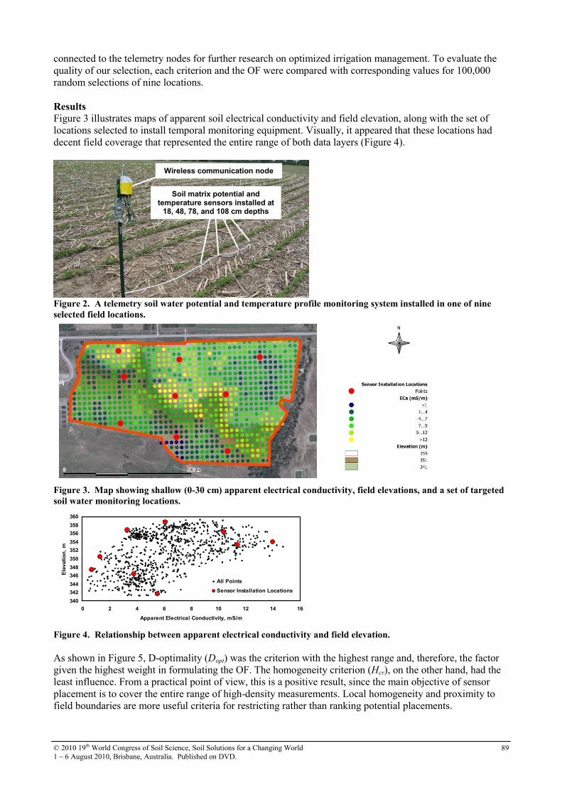
© 2010 19th World Congress of Soil Science, Soil Solutions for a Changing World
1 – 6 August 2010, Brisbane, Australia. Published on DVD. 89
connected to the telemetry nodes for further research on optimized irrigation management. To evaluate the
quality of our selection, each criterion and the OF were compared with corresponding values for 100,000
random selections of nine locations.
Results Figure 3 illustrates maps of apparent soil electrical conductivity and field elevation, along with the set of
locations selected to install temporal monitoring equipment. Visually, it appeared that these locations had
decent field coverage that represented the entire range of both data layers (Figure 4).
Figure 2. A telemetry soil water potential and temperature profile monitoring system installed in one of nine
selected field locations.
Figure 3. Map showing shallow (0-30 cm) apparent electrical conductivity, field elevations, and a set of targeted
soil water monitoring locations.
340
342
344
346
348
350
352
354
356
358
360
0 2 4 6 8 10 12 14 16
Apparent Electrical Conductivity, mS/m
Elevation, m
All Points
Sensor Installation Locations
Figure 4. Relationship between apparent electrical conductivity and field elevation.
As shown in Figure 5, D-optimality (Dopt) was the criterion with the highest range and, therefore, the factor
given the highest weight in formulating the OF. The homogeneity criterion (Hcr), on the other hand, had the
least influence. From a practical point of view, this is a positive result, since the main objective of sensor
placement is to cover the entire range of high-density measurements. Local homogeneity and proximity to
field boundaries are more useful criteria for restricting rather than ranking potential placements.
Soil matrix potential and temperature sensors installed at 18, 48, 78, and 108 cm depths
Wireless communication node

© 2010 19th World Congress of Soil Science, Soil Solutions for a Changing World
1 – 6 August 2010, Brisbane, Australia. Published on DVD. 90
0.0
1.0
2.0
3.0
4.0
5.0
Sopt Dopt (EC) Dopt
(Elevation)
Hcr (EC) Hcr (Elevation) OF
Optimality Criteria
Norm
alized Criteria Value
Median and Range
Sensor Installation Locations
Figure 5. Median and range of individual normalized criteria and OF values for 100,000 random soil water
monitoring selections, with actual installation and optimal sets of targeted points.
Although the set of monitoring locations with the highest value of the OF was one of 100,000 random
selections, it would be impractical to locate monitors based on this set, because some locations were in
restricted field areas (close to boundaries and pivot tracks). Avoiding such areas through manual intrusion
naturally decreased the values of the criteria as well as the overall OF. Although this reduction was not
significant, eliminating restricted parts of the field prior to the selection process might be appropriate in the
future.
Although Sopt and Dopt criteria are highly popular in spatial statistics, our definition of Hcr is quite vague. The
established criterion is well-defined for weighting power since only highly variable locations would reduce
otherwise high OF values. However, this does not consider the overall neighbourhood statistics. A more
involved homogeneity criterion will be considered in the future to restrict the consideration of relatively
small areas with apparent measurement stability, and to allow the selection of field areas with a directional
gradient of a given measurement.
Conclusion In this research, we proposed a method for comprehensive evaluation of soil monitoring site locations with
respect to multiple high-resolution sensor-based data layers. An objective function was developed
representing the entire range of sensor data spread across the field and local homogeneity. Partially
subjective selection of nine locations to install soil water potential and temperature monitoring equipment
was shown to provide a relatively high OF value that was, however, less than the maximum value for
100,000 random selections. A more involved process is needed that would automatically select the most
appropriate set of targeted sampling/monitoring locations.
Acknowledgement
This publication is a contribution of the University of Nebraska Agricultural Research Division, supported in
part by funds provided through Nebraska Centre for Energy Science Research through the Water, Energy
and Agriculture Initiative (WEAI).
References Brus DJ, Heuvelink GBM (2007) Optimization of sample patterns for universal kriging of environmental
variables. Geoderma 138, 86-95.
de Gruijter JJ, McBratney AB, Taylor J (2008) Sampling for high resolution soil mapping. In ‘Proceedings
of the First Global Workshop on High Resolution Digital Soil Sensing and Mapping’ (The University
of Sydney: Australia, Sydney).
Lesch SM. 2005. Sensor-directed spatial response surface sampling designs for characterizing spatial
variation in soil properties. Computers and Electronics in Agriculture 46, 153-180.
Minasny B, McBratney AB (2006) A conditioned Latin hypercube method for sampling in the presence of
ancillary information. Computers and Geosciences 32, 1378-1388.
SAS (2008) Optimality criteria. In ‘SAS/QC User's Guide’ (SAS Institute, Inc: Cary, North Carolina).
Sadler EJ, Evans RG, Stone KC, Camp CR (2005) Opportunities for conservation with precision irrigation.
Journal of Soil and Water Conservation 60, 371-379.

© 2010 19th World Congress of Soil Science, Soil Solutions for a Changing World
1 – 6 August 2010, Brisbane, Australia. Published on DVD. 91
Mapping the information content of Australian visible-near infrared soil spectra
R.A. Viscarra Rossel
1*, A. Chappell
1, P. de Caritat
2, and N.J. McKenzie
1
1 CSIRO Land and Water, Soil and Landscape Science, GPO Box 1666 Canberra ACT 2601, Australia 2 Geoscience Australia, GPO Box 378, Canberra ACT 2601, Australia
Abstract We describe the information content of soil visible–near infrared (vis–NIR) reflectance spectra and map their
spatial distribution across Australia. The spectra of 4030 surface soil sample from across the country were
compressed using a principal component analysis (PCA) and the resulting scores were mapped by ordinary
point kriging. The largely dominant and common feature in the maps was the difference between the more
expansive, older and more weathered landscapes in the centre and west of Australia and the generally
younger, more complex landscapes in the east. A surface soil class map derived from the clustering of the
principal components was similar to an existing soil classification map. Visible–NIR reflectance spectra
provide an integrative measure to rapidly and efficiently measure the constituents of the soil. It can replace
the use of traditional soil properties to describe the soil and make geomorphological interpretations of its
spatial distribution and therefore it can be used to classify soil objectively.
Key Words Reflectance spectra, visible–near infrared, kriging, Australian soil.
Introduction Recent technological advances in computing and measurement technologies are providing soil scientists with
tools that can be used to improve the efficiency of soil measurements. Over approximately the last three
decades and across diverse fields of research from remote sensing to chemometrics, interest has developed in
the rapid, non-destructive measurements of the intrinsic optical properties of the soil in the visible–near
infrared (vis–NIR) and mid-infrared (mid-IR) ranges of the electromagnetic spectrum between 400 and 2500
nm and 2500 nm and 25,000 nm, respectively (e.g. Ben-Dor et al. 1999). Although mid-IR soil spectra has a
stronger signal, the advantages of the vis-NIR are: the analysis requires less sample preparation, the
instrumentation is portable and can be easily used in the field, direct links can be made with hyperspectral
remote sensing (e.g. Gomez et al. 2008) and iron oxides, clay minerals and soil colour can be easily
measured directly from the spectra (Viscarra Rossel et al. 2009).
Field and laboratory experiments have shown that wavelength-specific absorptions of electromagnetic
radiation in the vis–NIR provide diagnostic reflectance spectra for the chemical, physical and mineralogical
composition of the soil. For example, broad and shallow absorption bands in wavelengths smaller than 1000
nm can be due to iron oxides; narrow, well-defined absorptions near 1400 nm and 1900 nm can be related to
hydroxyl and water; absorptions near 2200 nm to clay minerals; and various absorptions throughout the
spectrum to organic matter.
We propose that spectra: (a) provide an integrative measure that can be used to rapidly and efficiently
measure the constitution of the soil, and (b) spectra can replace the use of traditional soil properties for
describing the soil and making geomorphological interpretations of its spatial distribution. To support our
proposal, we describe the information content of Australian soil vis–NIR spectra and map its spatial
distribution across Australia.
Methods Soil samples
The soil samples used here originated from different sources, comprising continental, regional and field scale
soil surveys. The samples were from: (i) the Australian Commonwealth Scientific and Industrial Research
Organisation’s (CSIRO) National Soil Archive, (ii) The National Geochemical Survey of Australia (NGSA),
(iii) state department and regional surveys and (iv) a number smaller surveys conducted for research into
precision agriculture. Their spatial distribution is shown in Figure 1. The samples cover the range of
Australian soil orders (Isbell 1996) over the varying climatic regimes across Australia (Figure 1). All 4030
samples were air dry and approximately 100 g subsamples were passed through a 2 mm sieve for the
spectroscopic analysis.

© 2010 19th World Congress of Soil Science, Soil Solutions for a Changing World
1 – 6 August 2010, Brisbane, Australia. Published on DVD. 92
Figure 1. Spatial distribution of the data. The different symbols indicate their origin: CSIRO National Soil
Archive (C), The National Geochemical Survey of Australia (NGSA) (G), state department surveys from
Queensland (Q) and Wester Australia (WA) and other regional and field scale surveys (O).
Vis-NIR spectroscopy and spectroscopic analyses
The diffuse reflectance spectra of the 4030 soil samples were measured using the Labspec® vis-NIR
spectrometer (Analytical Spectral Devices, Bolder, Colorado, USA) with a spectral range of 350–2500 nm.
The soils were measured using a contact probe (Analytical Spectral Devices, Bolder, Colorado, USA) and a
Spectralon® panel was used to obtain a white reference once every 10 measurements. For each soil
measurement, 30 spectra were averaged to improve the signal-to-noise ratio. Spectra were collected with a
sampling resolution of 1 nm so that each spectrum was made up of 2151 wavelengths.
A continuum removal technique (Clark and Roush 1984) was used to isolate absorption features in the
spectra. We calculated the continuum-removed (CR) spectrum by dividing the original reflectance values by
the corresponding values of the continuum line.
Multivariate statistical analysis
The continuum-removed (CR) spectra were mean-centred and then analysed using principal component
analysis (PCA). We used both the scores and loadings to interpret our data. To provide a more general
description of the 4030 soil samples, the first four principal component scores (which accounted for 98% of
the variance in the data) were clustered using the k-means algorithm. A scree plot of the percent variance
explained by cluster was used to select the number of clusters. The spatial distribution of the clusters was
plotted and the absorption features of the average spectrum of each of cluster were used to interpret the soil
samples.
Geostatistical analyses and mapping
We computed experimental variograms for the scores of each of the first three principal components. We
fitted, using weighted least squares, a number of different models to our data (spherical, exponential,
Matern), including models that describe a nested combination of two individual variograms (Webster &
Oliver 2001). The rationale for fitting nested models was that soil variability can often be described by a
combination of different processes, one nested within another and acting at different spatial scales. We used
the Akaike Information Criterion (AIC) (Akaike 1973) to select the best, most parsimonious model. The
model with the best least squares fit to the experimental semi-variances of the scores, for the first three
principal components, was a nested exponential model with a nugget effect. We used ordinary point kriging
(Webster & Oliver 2001) to map the spatial distribution of each of the first three principal component scores
across Australia on a 5 km square grid. The kriged principal component scores surfaces were clustered using
the k-means technique. This resulted in a classed map of surface soil characteristics across Australia.
Results Mapping the information content of soil vis-NIR spectra
The variograms of the principal components are shown in Figure 2. The semi-variances in the first principal
component (PC) are larger than those in the other PCs and explain a larger proportion of the spatially
dependent variation. However, the variograms of PC two and three also demonstrate good spatial
dependence, the nested exponential models provide a good fit (Figure 2) and the loadings spectra show
strong and clearly identifiable features (Figure 3) that contribute to the interpretation of Australian soil.
Therefore we retained them in the analysis.
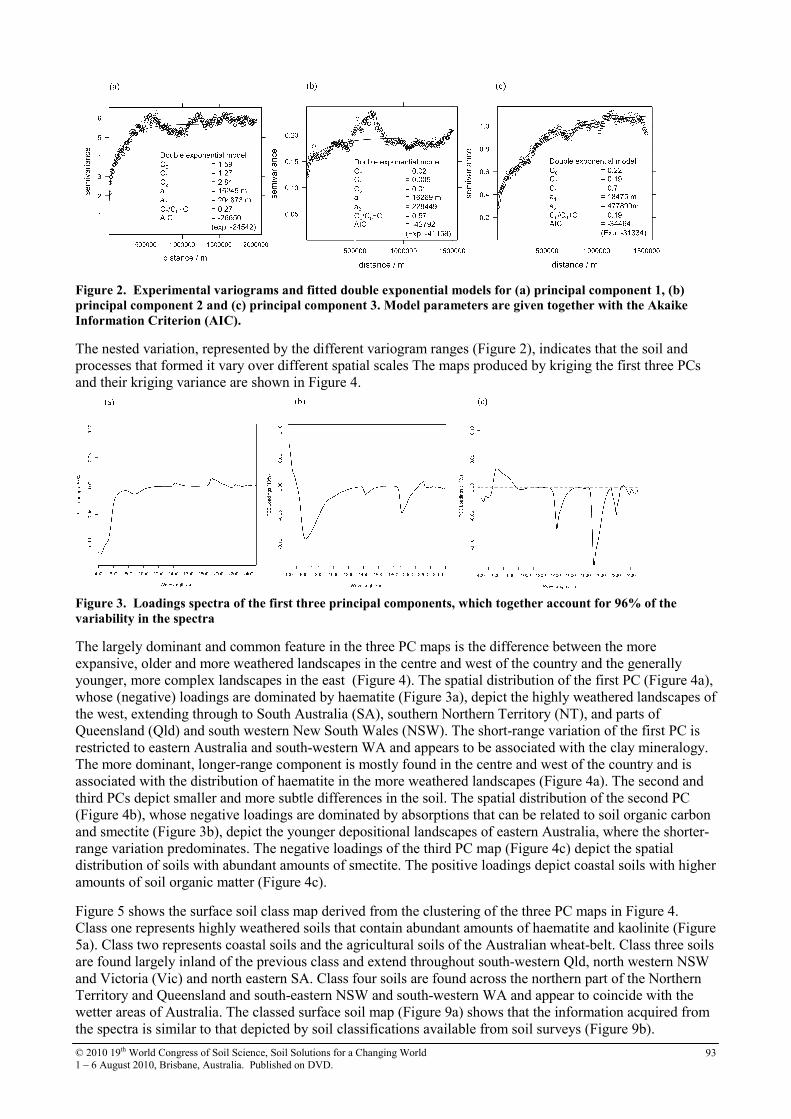
© 2010 19th World Congress of Soil Science, Soil Solutions for a Changing World
1 – 6 August 2010, Brisbane, Australia. Published on DVD. 93
Figure 2. Experimental variograms and fitted double exponential models for (a) principal component 1, (b)
principal component 2 and (c) principal component 3. Model parameters are given together with the Akaike
Information Criterion (AIC).
The nested variation, represented by the different variogram ranges (Figure 2), indicates that the soil and
processes that formed it vary over different spatial scales The maps produced by kriging the first three PCs
and their kriging variance are shown in Figure 4.
Figure 3. Loadings spectra of the first three principal components, which together account for 96% of the
variability in the spectra
The largely dominant and common feature in the three PC maps is the difference between the more
expansive, older and more weathered landscapes in the centre and west of the country and the generally
younger, more complex landscapes in the east (Figure 4). The spatial distribution of the first PC (Figure 4a),
whose (negative) loadings are dominated by haematite (Figure 3a), depict the highly weathered landscapes of
the west, extending through to South Australia (SA), southern Northern Territory (NT), and parts of
Queensland (Qld) and south western New South Wales (NSW). The short-range variation of the first PC is
restricted to eastern Australia and south-western WA and appears to be associated with the clay mineralogy.
The more dominant, longer-range component is mostly found in the centre and west of the country and is
associated with the distribution of haematite in the more weathered landscapes (Figure 4a). The second and
third PCs depict smaller and more subtle differences in the soil. The spatial distribution of the second PC
(Figure 4b), whose negative loadings are dominated by absorptions that can be related to soil organic carbon
and smectite (Figure 3b), depict the younger depositional landscapes of eastern Australia, where the shorter-
range variation predominates. The negative loadings of the third PC map (Figure 4c) depict the spatial
distribution of soils with abundant amounts of smectite. The positive loadings depict coastal soils with higher
amounts of soil organic matter (Figure 4c).
Figure 5 shows the surface soil class map derived from the clustering of the three PC maps in Figure 4.
Class one represents highly weathered soils that contain abundant amounts of haematite and kaolinite (Figure
5a). Class two represents coastal soils and the agricultural soils of the Australian wheat-belt. Class three soils
are found largely inland of the previous class and extend throughout south-western Qld, north western NSW
and Victoria (Vic) and north eastern SA. Class four soils are found across the northern part of the Northern
Territory and Queensland and south-eastern NSW and south-western WA and appear to coincide with the
wetter areas of Australia. The classed surface soil map (Figure 9a) shows that the information acquired from
the spectra is similar to that depicted by soil classifications available from soil surveys (Figure 9b).
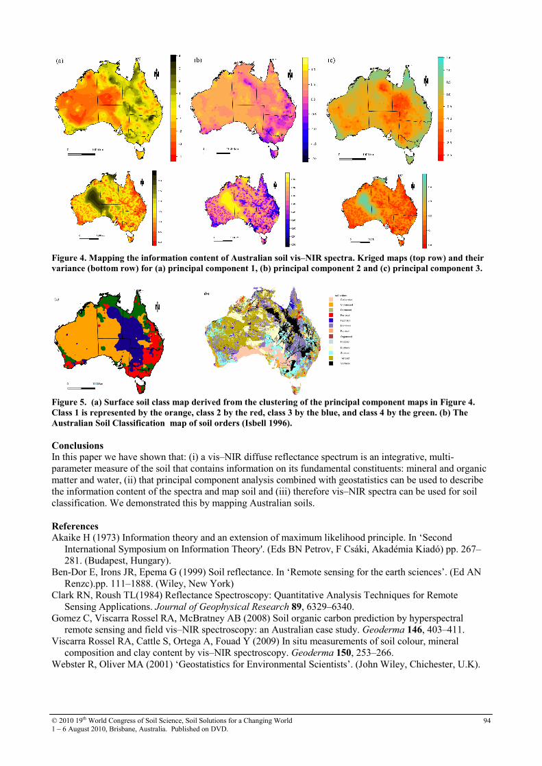
© 2010 19th World Congress of Soil Science, Soil Solutions for a Changing World
1 – 6 August 2010, Brisbane, Australia. Published on DVD. 94
Figure 4. Mapping the information content of Australian soil vis–NIR spectra. Kriged maps (top row) and their
variance (bottom row) for (a) principal component 1, (b) principal component 2 and (c) principal component 3.
Figure 5. (a) Surface soil class map derived from the clustering of the principal component maps in Figure 4.
Class 1 is represented by the orange, class 2 by the red, class 3 by the blue, and class 4 by the green. (b) The
Australian Soil Classification map of soil orders (Isbell 1996).
Conclusions In this paper we have shown that: (i) a vis–NIR diffuse reflectance spectrum is an integrative, multi-
parameter measure of the soil that contains information on its fundamental constituents: mineral and organic
matter and water, (ii) that principal component analysis combined with geostatistics can be used to describe
the information content of the spectra and map soil and (iii) therefore vis–NIR spectra can be used for soil
classification. We demonstrated this by mapping Australian soils.
References Akaike H (1973) Information theory and an extension of maximum likelihood principle. In ‘Second
International Symposium on Information Theory'. (Eds BN Petrov, F Csáki, Akadémia Kiadó) pp. 267–
281. (Budapest, Hungary).
Ben-Dor E, Irons JR, Epema G (1999) Soil reflectance. In ‘Remote sensing for the earth sciences’. (Ed AN
Renzc).pp. 111–1888. (Wiley, New York)
Clark RN, Roush TL(1984) Reflectance Spectroscopy: Quantitative Analysis Techniques for Remote
Sensing Applications. Journal of Geophysical Research 89, 6329–6340.
Gomez C, Viscarra Rossel RA, McBratney AB (2008) Soil organic carbon prediction by hyperspectral
remote sensing and field vis–NIR spectroscopy: an Australian case study. Geoderma 146, 403–411.
Viscarra Rossel RA, Cattle S, Ortega A, Fouad Y (2009) In situ measurements of soil colour, mineral
composition and clay content by vis–NIR spectroscopy. Geoderma 150, 253–266.
Webster R, Oliver MA (2001) ‘Geostatistics for Environmental Scientists’. (John Wiley, Chichester, U.K).
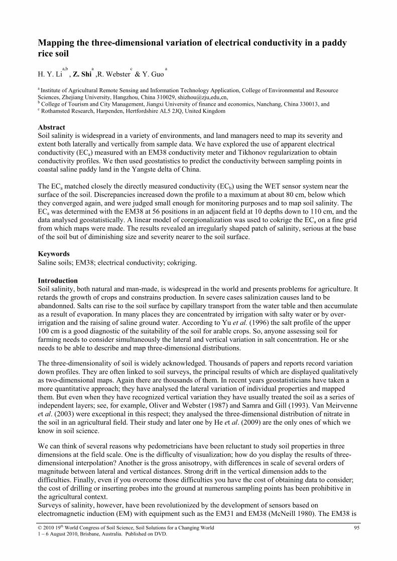
© 2010 19th World Congress of Soil Science, Soil Solutions for a Changing World
1 – 6 August 2010, Brisbane, Australia. Published on DVD. 95
Mapping the three-dimensional variation of electrical conductivity in a paddy
rice soil
H. Y. Lia,b
, Z. Shia
,R. Websterc
& Y. Guo a
a Institute of Agricultural Remote Sensing and Information Technology Application, College of Environmental and Resource
Sciences, Zhejiang University, Hangzhou, China 310029, shizhou@zju,edu,cn, b College of Tourism and City Management, Jiangxi University of finance and economics, Nanchang, China 330013, and c Rothamsted Research, Harpenden, Hertfordshire AL5 2JQ, United Kingdom
Abstract Soil salinity is widespread in a variety of environments, and land managers need to map its severity and
extent both laterally and vertically from sample data. We have explored the use of apparent electrical
conductivity (ECa) measured with an EM38 conductivity meter and Tikhonov regularization to obtain
conductivity profiles. We then used geostatistics to predict the conductivity between sampling points in
coastal saline paddy land in the Yangste delta of China.
The ECa matched closely the directly measured conductivity (ECb) using the WET sensor system near the
surface of the soil. Discrepancies increased down the profile to a maximum at about 80 cm, below which
they converged again, and were judged small enough for monitoring purposes and to map soil salinity. The
ECa was determined with the EM38 at 56 positions in an adjacent field at 10 depths down to 110 cm, and the
data analysed geostatistically. A linear model of coregionalization was used to cokrige the ECa on a fine grid
from which maps were made. The results revealed an irregularly shaped patch of salinity, serious at the base
of the soil but of diminishing size and severity nearer to the soil surface.
Keywords
Saline soils; EM38; electrical conductivity; cokriging.
Introduction Soil salinity, both natural and man-made, is widespread in the world and presents problems for agriculture. It
retards the growth of crops and constrains production. In severe cases salinization causes land to be
abandonned. Salts can rise to the soil surface by capillary transport from the water table and then accumulate
as a result of evaporation. In many places they are concentrated by irrigation with salty water or by over-
irrigation and the raising of saline ground water. According to Yu et al. (1996) the salt profile of the upper
100 cm is a good diagnostic of the suitability of the soil for arable crops. So, anyone assessing soil for
farming needs to consider simultaneously the lateral and vertical variation in salt concentration. He or she
needs to be able to describe and map three-dimensional distributions.
The three-dimensionality of soil is widely acknowledged. Thousands of papers and reports record variation
down profiles. They are often linked to soil surveys, the principal results of which are displayed qualitatively
as two-dimensional maps. Again there are thousands of them. In recent years geostatisticians have taken a
more quantitative approach; they have analysed the lateral variation of individual properties and mapped
them. But even when they have recognized vertical variation they have usually treated the soil as a series of
independent layers; see, for example, Oliver and Webster (1987) and Samra and Gill (1993). Van Meirvenne
et al. (2003) were exceptional in this respect; they analysed the three-dimensional distribution of nitrate in
the soil in an agricultural field. Their study and later one by He et al. (2009) are the only ones of which we
know in soil science.
We can think of several reasons why pedometricians have been reluctant to study soil properties in three
dimensions at the field scale. One is the difficulty of visualization; how do you display the results of three-
dimensional interpolation? Another is the gross anisotropy, with differences in scale of several orders of
magnitude between lateral and vertical distances. Strong drift in the vertical dimension adds to the
difficulties. Finally, even if you overcome those difficulties you have the cost of obtaining data to consider;
the cost of drilling or inserting probes into the ground at numerous sampling points has been prohibitive in
the agricultural context.
Surveys of salinity, however, have been revolutionized by the development of sensors based on
electromagnetic induction (EM) with equipment such as the EM31 and EM38 (McNeill 1980). The EM38 is
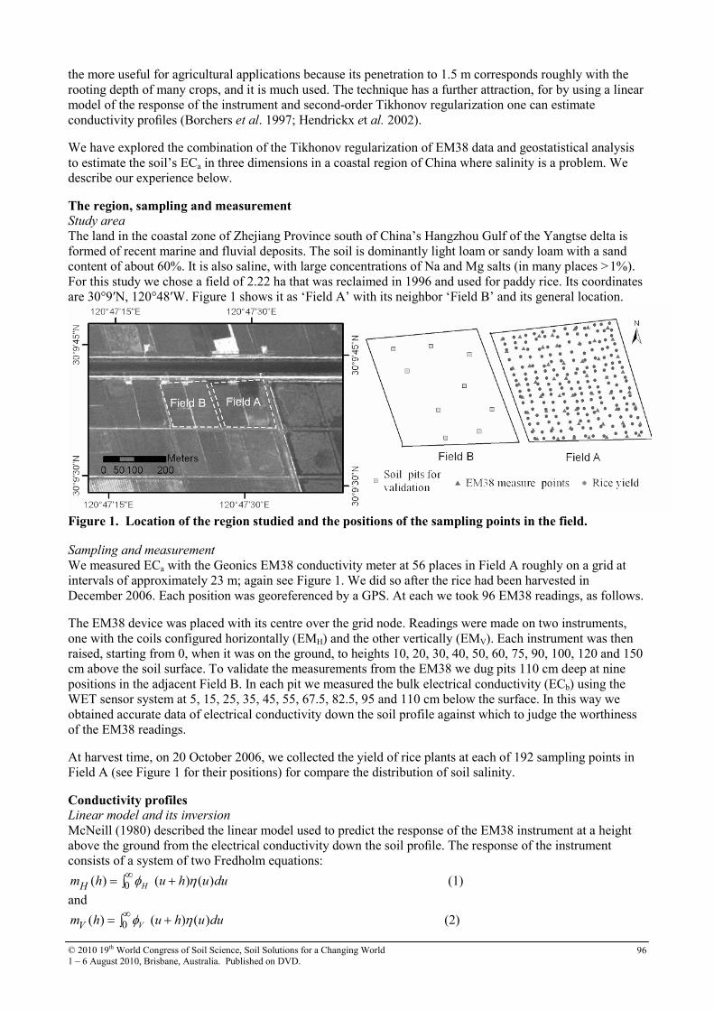
© 2010 19th World Congress of Soil Science, Soil Solutions for a Changing World
1 – 6 August 2010, Brisbane, Australia. Published on DVD. 96
the more useful for agricultural applications because its penetration to 1.5 m corresponds roughly with the
rooting depth of many crops, and it is much used. The technique has a further attraction, for by using a linear
model of the response of the instrument and second-order Tikhonov regularization one can estimate
conductivity profiles (Borchers et al. 1997; Hendrickx et al. 2002).
We have explored the combination of the Tikhonov regularization of EM38 data and geostatistical analysis
to estimate the soil’s ECa in three dimensions in a coastal region of China where salinity is a problem. We
describe our experience below.
The region, sampling and measurement Study area
The land in the coastal zone of Zhejiang Province south of China’s Hangzhou Gulf of the Yangtse delta is
formed of recent marine and fluvial deposits. The soil is dominantly light loam or sandy loam with a sand
content of about 60%. It is also saline, with large concentrations of Na and Mg salts (in many places >1%).
For this study we chose a field of 2.22 ha that was reclaimed in 1996 and used for paddy rice. Its coordinates
are 30°9′N, 120°48′W. Figure 1 shows it as ‘Field A’ with its neighbor ‘Field B’ and its general location.
Figure 1. Location of the region studied and the positions of the sampling points in the field.
Sampling and measurement
We measured ECa with the Geonics EM38 conductivity meter at 56 places in Field A roughly on a grid at
intervals of approximately 23 m; again see Figure 1. We did so after the rice had been harvested in
December 2006. Each position was georeferenced by a GPS. At each we took 96 EM38 readings, as follows.
The EM38 device was placed with its centre over the grid node. Readings were made on two instruments,
one with the coils configured horizontally (EMH) and the other vertically (EMV). Each instrument was then
raised, starting from 0, when it was on the ground, to heights 10, 20, 30, 40, 50, 60, 75, 90, 100, 120 and 150
cm above the soil surface. To validate the measurements from the EM38 we dug pits 110 cm deep at nine
positions in the adjacent Field B. In each pit we measured the bulk electrical conductivity (ECb) using the
WET sensor system at 5, 15, 25, 35, 45, 55, 67.5, 82.5, 95 and 110 cm below the surface. In this way we
obtained accurate data of electrical conductivity down the soil profile against which to judge the worthiness
of the EM38 readings.
At harvest time, on 20 October 2006, we collected the yield of rice plants at each of 192 sampling points in
Field A (see Figure 1 for their positions) for compare the distribution of soil salinity.
Conductivity profiles Linear model and its inversion
McNeill (1980) described the linear model used to predict the response of the EM38 instrument at a height
above the ground from the electrical conductivity down the soil profile. The response of the instrument
consists of a system of two Fredholm equations:
0( ) ( ) ( )HHm h u h u duφ η∞= +∫ (1)
and
0( ) ( ) ( )VVm h u h u duφ η∞= +∫ (2)
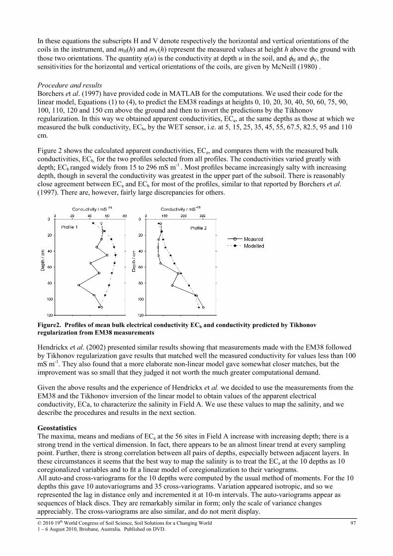
© 2010 19th World Congress of Soil Science, Soil Solutions for a Changing World
1 – 6 August 2010, Brisbane, Australia. Published on DVD. 97
In these equations the subscripts H and V denote respectively the horizontal and vertical orientations of the
coils in the instrument, and mH(h) and mV(h) represent the measured values at height h above the ground with
those two orientations. The quantity η(u) is the conductivity at depth u in the soil, and φH and φV, the
sensitivities for the horizontal and vertical orientations of the coils, are given by McNeill (1980) .
Procedure and results
Borchers et al. (1997) have provided code in MATLAB for the computations. We used their code for the
linear model, Equations (1) to (4), to predict the EM38 readings at heights 0, 10, 20, 30, 40, 50, 60, 75, 90,
100, 110, 120 and 150 cm above the ground and then to invert the predictions by the Tikhonov
regularization. In this way we obtained apparent conductivities, ECa, at the same depths as those at which we
measured the bulk conductivity, ECb, by the WET sensor, i.e. at 5, 15, 25, 35, 45, 55, 67.5, 82.5, 95 and 110
cm.
Figure 2 shows the calculated apparent conductivities, ECa, and compares them with the measured bulk
conductivities, ECb, for the two profiles selected from all profiles. The conductivities varied greatly with
depth; ECb ranged widely from 15 to 296 mS m-1
. Most profiles became increasingly salty with increasing
depth, though in several the conductivity was greatest in the upper part of the subsoil. There is reasonably
close agreement between ECa and ECb for most of the profiles, similar to that reported by Borchers et al.
(1997). There are, however, fairly large discrepancies for others.
Figure2. Profiles of mean bulk electrical conductivity ECb and conductivity predicted by Tikhonov
regularization from EM38 measurements
Hendrickx et al. (2002) presented similar results showing that measurements made with the EM38 followed
by Tikhonov regularization gave results that matched well the measured conductivity for values less than 100
mS m-1
. They also found that a more elaborate non-linear model gave somewhat closer matches, but the
improvement was so small that they judged it not worth the much greater computational demand.
Given the above results and the experience of Hendrickx et al. we decided to use the measurements from the
EM38 and the Tikhonov inversion of the linear model to obtain values of the apparent electrical
conductivity, ECa, to characterize the salinity in Field A. We use these values to map the salinity, and we
describe the procedures and results in the next section.
Geostatistics The maxima, means and medians of ECa at the 56 sites in Field A increase with increasing depth; there is a
strong trend in the vertical dimension. In fact, there appears to be an almost linear trend at every sampling
point. Further, there is strong correlation between all pairs of depths, especially between adjacent layers. In
these circumstances it seems that the best way to map the salinity is to treat the ECa at the 10 depths as 10
coregionalized variables and to fit a linear model of coregionalization to their variograms.
All auto-and cross-variograms for the 10 depths were computed by the usual method of moments. For the 10
depths this gave 10 autovariograms and 35 cross-variograms. Variation appeared isotropic, and so we
represented the lag in distance only and incremented it at 10-m intervals. The auto-variograms appear as
sequences of black discs. They are remarkably similar in form; only the scale of variance changes
appreciably. The cross-variograms are also similar, and do not merit display.
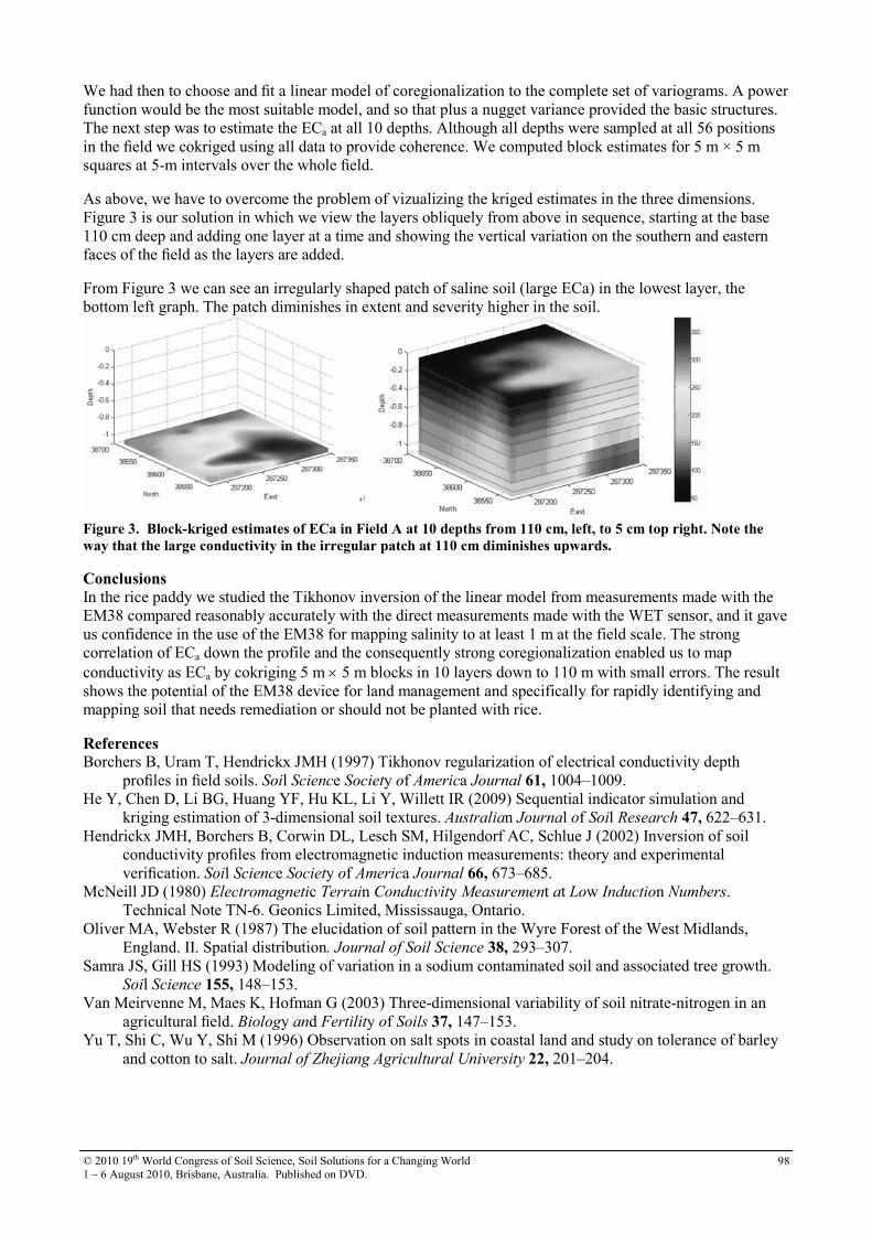
© 2010 19th World Congress of Soil Science, Soil Solutions for a Changing World
1 – 6 August 2010, Brisbane, Australia. Published on DVD. 98
We had then to choose and fit a linear model of coregionalization to the complete set of variograms. A power
function would be the most suitable model, and so that plus a nugget variance provided the basic structures.
The next step was to estimate the ECa at all 10 depths. Although all depths were sampled at all 56 positions
in the field we cokriged using all data to provide coherence. We computed block estimates for 5 m × 5 m
squares at 5-m intervals over the whole field.
As above, we have to overcome the problem of vizualizing the kriged estimates in the three dimensions.
Figure 3 is our solution in which we view the layers obliquely from above in sequence, starting at the base
110 cm deep and adding one layer at a time and showing the vertical variation on the southern and eastern
faces of the field as the layers are added.
From Figure 3 we can see an irregularly shaped patch of saline soil (large ECa) in the lowest layer, the
bottom left graph. The patch diminishes in extent and severity higher in the soil.
Figure 3. Block-kriged estimates of ECa in Field A at 10 depths from 110 cm, left, to 5 cm top right. Note the
way that the large conductivity in the irregular patch at 110 cm diminishes upwards.
Conclusions In the rice paddy we studied the Tikhonov inversion of the linear model from measurements made with the
EM38 compared reasonably accurately with the direct measurements made with the WET sensor, and it gave
us confidence in the use of the EM38 for mapping salinity to at least 1 m at the field scale. The strong
correlation of ECa down the profile and the consequently strong coregionalization enabled us to map
conductivity as ECa by cokriging 5 m × 5 m blocks in 10 layers down to 110 m with small errors. The result
shows the potential of the EM38 device for land management and specifically for rapidly identifying and
mapping soil that needs remediation or should not be planted with rice.
References Borchers B, Uram T, Hendrickx JMH (1997) Tikhonov regularization of electrical conductivity depth
profiles in field soils. Soil Science Society of America Journal 61, 1004–1009.
He Y, Chen D, Li BG, Huang YF, Hu KL, Li Y, Willett IR (2009) Sequential indicator simulation and
kriging estimation of 3-dimensional soil textures. Australian Journal of Soil Research 47, 622–631.
Hendrickx JMH, Borchers B, Corwin DL, Lesch SM, Hilgendorf AC, Schlue J (2002) Inversion of soil
conductivity profiles from electromagnetic induction measurements: theory and experimental
verification. Soil Science Society of America Journal 66, 673–685.
McNeill JD (1980) Electromagnetic Terrain Conductivity Measurement at Low Induction Numbers.
Technical Note TN-6. Geonics Limited, Mississauga, Ontario.
Oliver MA, Webster R (1987) The elucidation of soil pattern in the Wyre Forest of the West Midlands,
England. II. Spatial distribution. Journal of Soil Science 38, 293–307.
Samra JS, Gill HS (1993) Modeling of variation in a sodium contaminated soil and associated tree growth.
Soil Science 155, 148–153.
Van Meirvenne M, Maes K, Hofman G (2003) Three-dimensional variability of soil nitrate-nitrogen in an
agricultural field. Biology and Fertility of Soils 37, 147–153.
Yu T, Shi C, Wu Y, Shi M (1996) Observation on salt spots in coastal land and study on tolerance of barley
and cotton to salt. Journal of Zhejiang Agricultural University 22, 201–204.
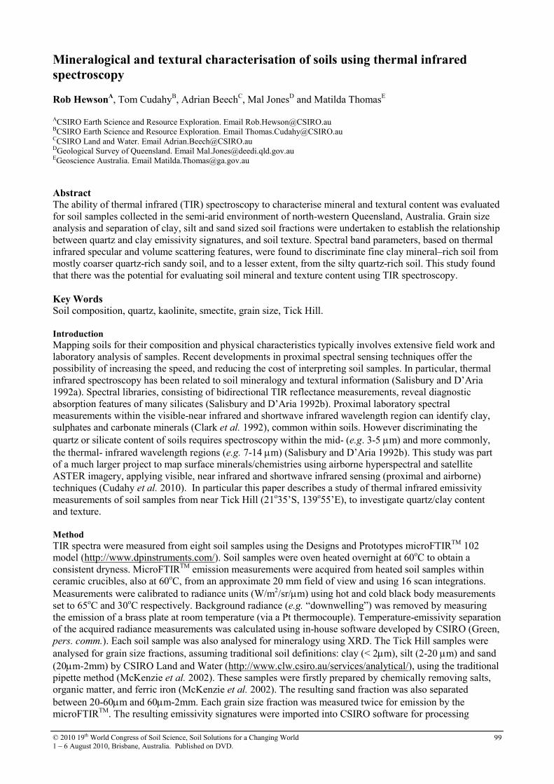
© 2010 19th World Congress of Soil Science, Soil Solutions for a Changing World
1 – 6 August 2010, Brisbane, Australia. Published on DVD. 99
Mineralogical and textural characterisation of soils using thermal infrared
spectroscopy
Rob HewsonA, Tom Cudahy
B, Adrian Beech
C, Mal Jones
D and Matilda Thomas
E
ACSIRO Earth Science and Resource Exploration. Email [email protected] BCSIRO Earth Science and Resource Exploration. Email [email protected] CCSIRO Land and Water. Email [email protected] DGeological Survey of Queensland. Email [email protected] EGeoscience Australia. Email [email protected]
Abstract The ability of thermal infrared (TIR) spectroscopy to characterise mineral and textural content was evaluated
for soil samples collected in the semi-arid environment of north-western Queensland, Australia. Grain size
analysis and separation of clay, silt and sand sized soil fractions were undertaken to establish the relationship
between quartz and clay emissivity signatures, and soil texture. Spectral band parameters, based on thermal
infrared specular and volume scattering features, were found to discriminate fine clay mineral–rich soil from
mostly coarser quartz-rich sandy soil, and to a lesser extent, from the silty quartz-rich soil. This study found
that there was the potential for evaluating soil mineral and texture content using TIR spectroscopy.
Key Words Soil composition, quartz, kaolinite, smectite, grain size, Tick Hill.
Introduction
Mapping soils for their composition and physical characteristics typically involves extensive field work and
laboratory analysis of samples. Recent developments in proximal spectral sensing techniques offer the
possibility of increasing the speed, and reducing the cost of interpreting soil samples. In particular, thermal
infrared spectroscopy has been related to soil mineralogy and textural information (Salisbury and D’Aria
1992a). Spectral libraries, consisting of bidirectional TIR reflectance measurements, reveal diagnostic
absorption features of many silicates (Salisbury and D’Aria 1992b). Proximal laboratory spectral
measurements within the visible-near infrared and shortwave infrared wavelength region can identify clay,
sulphates and carbonate minerals (Clark et al. 1992), common within soils. However discriminating the
quartz or silicate content of soils requires spectroscopy within the mid- (e.g. 3-5 µm) and more commonly,
the thermal- infrared wavelength regions (e.g. 7-14 µm) (Salisbury and D’Aria 1992b). This study was part
of a much larger project to map surface minerals/chemistries using airborne hyperspectral and satellite
ASTER imagery, applying visible, near infrared and shortwave infrared sensing (proximal and airborne)
techniques (Cudahy et al. 2010). In particular this paper describes a study of thermal infrared emissivity
measurements of soil samples from near Tick Hill (21o35’S, 139
o55’E), to investigate quartz/clay content
and texture.
Method
TIR spectra were measured from eight soil samples using the Designs and Prototypes microFTIRTM
102
model (http://www.dpinstruments.com/). Soil samples were oven heated overnight at 60oC to obtain a
consistent dryness. MicroFTIRTM
emission measurements were acquired from heated soil samples within
ceramic crucibles, also at 60oC, from an approximate 20 mm field of view and using 16 scan integrations.
Measurements were calibrated to radiance units (W/m2/sr/µm) using hot and cold black body measurements
set to 65oC and 30
oC respectively. Background radiance (e.g. “downwelling”) was removed by measuring
the emission of a brass plate at room temperature (via a Pt thermocouple). Temperature-emissivity separation
of the acquired radiance measurements was calculated using in-house software developed by CSIRO (Green,
pers. comm.). Each soil sample was also analysed for mineralogy using XRD. The Tick Hill samples were
analysed for grain size fractions, assuming traditional soil definitions: clay (< 2µm), silt (2-20 µm) and sand
(20µm-2mm) by CSIRO Land and Water (http://www.clw.csiro.au/services/analytical/), using the traditional
pipette method (McKenzie et al. 2002). These samples were firstly prepared by chemically removing salts,
organic matter, and ferric iron (McKenzie et al. 2002). The resulting sand fraction was also separated
between 20-60µm and 60µm-2mm. Each grain size fraction was measured twice for emission by the
microFTIRTM
. The resulting emissivity signatures were imported into CSIRO software for processing
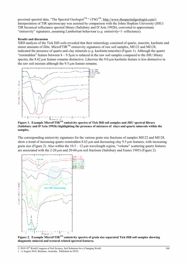
© 2010 19th World Congress of Soil Science, Soil Solutions for a Changing World
1 – 6 August 2010, Brisbane, Australia. Published on DVD. 100
proximal spectral data, “The Spectral GeologistTM
“ (TSGTM
, http://www.thespectralgeologist.com/).
Interpretation of TIR spectroscopy was assisted by comparison with the Johns Hopkins University (JHU)
TIR biconical reflectance spectral library (Salisbury and D’Aria 1992b), converted to approximate
“emissivity” signatures, assuming Lambertian behaviour (e.g. emissivity=1- reflectance).
Results and discussion
XRD analysis of the Tick Hill soils revealed that their mineralogy consisted of quartz, smectite, kaolinite and
minor amounts of illite. MicroFTIRTM
emissivity signatures of raw soil samples, MI122 and MI128,
indicated the presence of quartz and clay minerals (e.g. kaolinite/smectite) (Figure 1). Although the quartz
“reststrahlen” feature between 8 – 9.5µm is reduced in the raw soil samples compared to the JHU library
spectra, the 8.62 µm feature remains distinctive. Likewise the 9.0 µm kaolinite feature is less distinctive in
the raw soil mixture although the 9.5 µm feature remains.
Figure 1. Example MicroFTIR
TM emissivity spectra of Tick Hill soil samples and JHU spectral library
(Salisbury and D’Aria 1992b) highlighting the presence of mixtures of clays and quartz minerals within the
samples.
The corresponding emissivity signatures for the various grain size fractions of samples MI122 and MI128,
show a trend of increasing quartz reststrahlen 8.62 µm and decreasing clay 9.5 µm features, with increasing
grain size (Figure 2). Also within the 10.5 – 12 µm wavelength region, “volume” scattering quartz features
are associated with the 2-20 µm and 20-60 µm soil fractions (Salisbury and Eastes 1985) (Figure 2).
Figure 2. Example MicroFTIR
TM emissivity spectra of grain size separated Tick Hill soil samples showing
diagnostic mineral and textural related spectral features.
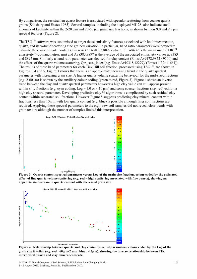
© 2010 19th World Congress of Soil Science, Soil Solutions for a Changing World
1 – 6 August 2010, Brisbane, Australia. Published on DVD. 101
By comparison, the reststrahlen quartz feature is associated with specular scattering from coarser quartz
grains (Salisbury and Eastes 1985). Several samples, including the displayed MI128, also indicate small
amounts of kaolinite within the 2-20 µm and 20-60 µm grain size fractions, as shown by their 9.0 and 9.8 µm
spectral features (Figure 2).
The TSGTM
software was customised to target those emissivity features associated with kaolinite/smectite,
quartz, and its volume scattering fine grained variation. In particular, band ratio parameters were devised to
estimate the coarser quartz content (Emiss8632 / Av8383,8897) where Emiss8632 is the mean microFTIRTM
emissivity (±30 nanometres, nm) and Av8383,8897 is the average of the associated emissivity values at 8383
and 8897 nm. Similarly a band ratio parameter was devised for clay content (EmissAv9178,9852 / 9500) and
the effects of fine quartz volume scattering, Qtz_scat._index (e.g. EmissAv10318,12279)/ (Emiss(1132+11664)).
The results of these band parameters for each Tick Hill soil fraction, processed using TSGTM
, are shown in
Figures 3, 4 and 5. Figure 3 shows that there is an approximate increasing trend in the quartz spectral
parameter with increasing grain size. A higher quartz volume scattering behaviour for the mid-sized fractions
(e.g. 2-60µm) is shown by the auxiliary colour coding (green to red, Figure 3). Figure 4 shows an inverse
trend between the clay and quartz spectral parameters however a high clay value can still appear present
within silty fractions (e.g. cyan coding, Log ~ 1.0 or ~ 10 µm) and some coarser fractions (e.g. red) exhibit a
high clay spectral parameter. Developing predictive clay % algorithms is complicated by such residual clay
content within separated soil fractions. However Figure 5 suggests predicting clay mineral content within
fractions less than 10 µm with low quartz content (e.g. blue) is possible although finer soil fractions are
required. Applying these spectral parameters to the eight raw soil samples did not reveal clear trends with
grain texture although the number of samples limited this interpretation.
Figure 3. Quartz content spectral parameter versus Log of the grain size fraction, colour coded by the estimated
effect of fine quartz volume scattering (e.g. red = high scattering associated with fine quartz), showing an
approximate decrease in quartz content with decreased grain size.
Figure 4. Relationship between quartz and clay content spectral parameters, colour coded by the Log of the
grain size fraction (e.g. red : 60 µµµµm-2 mm; blue : < 2µµµµm), showing the inverse relationship between TIR
interpreted quartz and clay mineral contents.
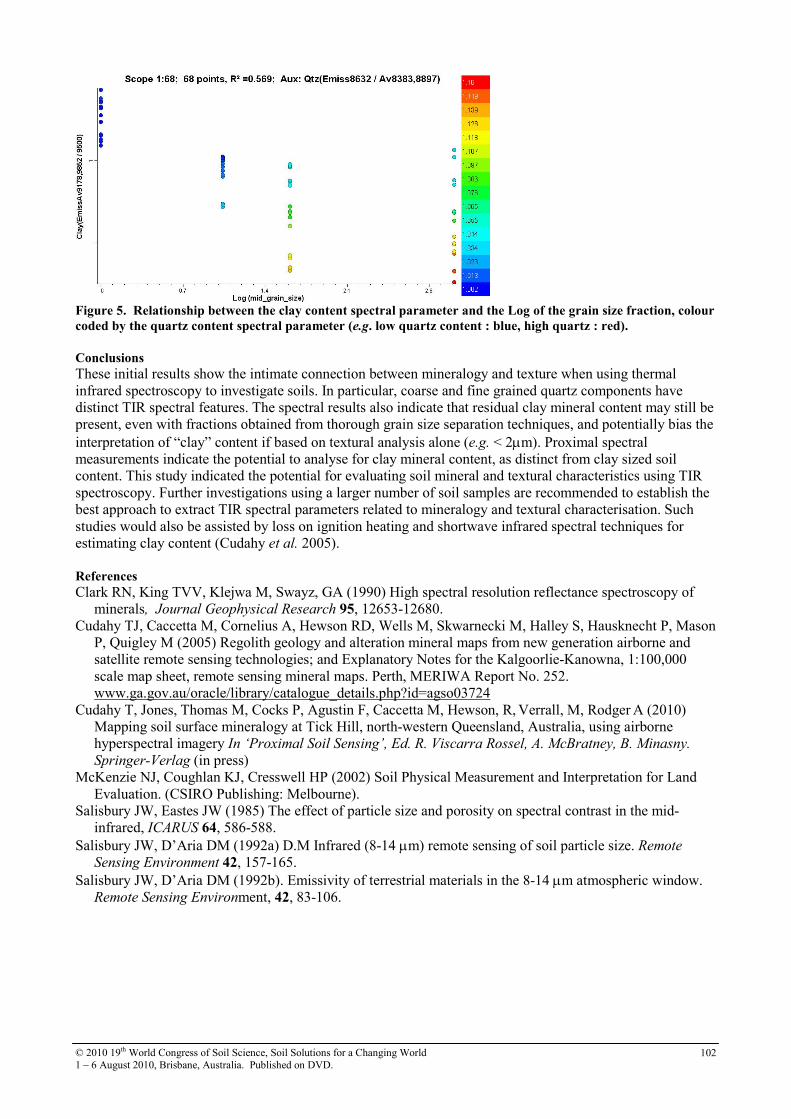
© 2010 19th World Congress of Soil Science, Soil Solutions for a Changing World
1 – 6 August 2010, Brisbane, Australia. Published on DVD. 102
Figure 5. Relationship between the clay content spectral parameter and the Log of the grain size fraction, colour
coded by the quartz content spectral parameter (e.g. low quartz content : blue, high quartz : red).
Conclusions
These initial results show the intimate connection between mineralogy and texture when using thermal
infrared spectroscopy to investigate soils. In particular, coarse and fine grained quartz components have
distinct TIR spectral features. The spectral results also indicate that residual clay mineral content may still be
present, even with fractions obtained from thorough grain size separation techniques, and potentially bias the
interpretation of “clay” content if based on textural analysis alone (e.g. < 2µm). Proximal spectral
measurements indicate the potential to analyse for clay mineral content, as distinct from clay sized soil
content. This study indicated the potential for evaluating soil mineral and textural characteristics using TIR
spectroscopy. Further investigations using a larger number of soil samples are recommended to establish the
best approach to extract TIR spectral parameters related to mineralogy and textural characterisation. Such
studies would also be assisted by loss on ignition heating and shortwave infrared spectral techniques for
estimating clay content (Cudahy et al. 2005).
References
Clark RN, King TVV, Klejwa M, Swayz, GA (1990) High spectral resolution reflectance spectroscopy of
minerals, Journal Geophysical Research 95, 12653-12680.
Cudahy TJ, Caccetta M, Cornelius A, Hewson RD, Wells M, Skwarnecki M, Halley S, Hausknecht P, Mason
P, Quigley M (2005) Regolith geology and alteration mineral maps from new generation airborne and
satellite remote sensing technologies; and Explanatory Notes for the Kalgoorlie-Kanowna, 1:100,000
scale map sheet, remote sensing mineral maps. Perth, MERIWA Report No. 252.
www.ga.gov.au/oracle/library/catalogue_details.php?id=agso03724
Cudahy T, Jones, Thomas M, Cocks P, Agustin F, Caccetta M, Hewson, R, Verrall, M, Rodger
A (2010)
Mapping soil surface mineralogy at Tick Hill, north-western Queensland, Australia, using airborne
hyperspectral imagery In ‘Proximal Soil Sensing’, Ed. R. Viscarra Rossel, A. McBratney, B. Minasny.
Springer-Verlag (in press)
McKenzie NJ, Coughlan KJ, Cresswell HP (2002) Soil Physical Measurement and Interpretation for Land
Evaluation. (CSIRO Publishing: Melbourne).
Salisbury JW, Eastes JW (1985) The effect of particle size and porosity on spectral contrast in the mid-
infrared, ICARUS 64, 586-588.
Salisbury JW, D’Aria DM (1992a) D.M Infrared (8-14 µm) remote sensing of soil particle size. Remote
Sensing Environment 42, 157-165.
Salisbury JW, D’Aria DM (1992b). Emissivity of terrestrial materials in the 8-14 µm atmospheric window.
Remote Sensing Environment, 42, 83-106.
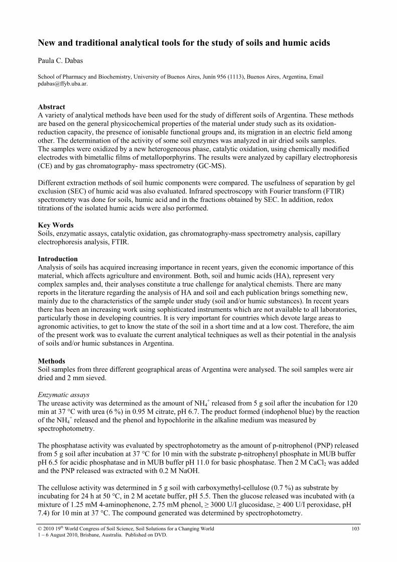
© 2010 19th World Congress of Soil Science, Soil Solutions for a Changing World
1 – 6 August 2010, Brisbane, Australia. Published on DVD. 103
New and traditional analytical tools for the study of soils and humic acids
Paula C. Dabas
School of Pharmacy and Biochemistry, University of Buenos Aires, Junín 956 (1113), Buenos Aires, Argentina, Email
Abstract A variety of analytical methods have been used for the study of different soils of Argentina. These methods
are based on the general physicochemical properties of the material under study such as its oxidation-
reduction capacity, the presence of ionisable functional groups and, its migration in an electric field among
other. The determination of the activity of some soil enzymes was analyzed in air dried soils samples.
The samples were oxidized by a new heterogeneous phase, catalytic oxidation, using chemically modified
electrodes with bimetallic films of metalloporphyrins. The results were analyzed by capillary electrophoresis
(CE) and by gas chromatography- mass spectrometry (GC-MS).
Different extraction methods of soil humic components were compared. The usefulness of separation by gel
exclusion (SEC) of humic acid was also evaluated. Infrared spectroscopy with Fourier transform (FTIR)
spectrometry was done for soils, humic acid and in the fractions obtained by SEC. In addition, redox
titrations of the isolated humic acids were also performed.
Key Words Soils, enzymatic assays, catalytic oxidation, gas chromatography-mass spectrometry analysis, capillary
electrophoresis analysis, FTIR.
Introduction Analysis of soils has acquired increasing importance in recent years, given the economic importance of this
material, which affects agriculture and environment. Both, soil and humic acids (HA), represent very
complex samples and, their analyses constitute a true challenge for analytical chemists. There are many
reports in the literature regarding the analysis of HA and soil and each publication brings something new,
mainly due to the characteristics of the sample under study (soil and/or humic substances). In recent years
there has been an increasing work using sophisticated instruments which are not available to all laboratories,
particularly those in developing countries. It is very important for countries which devote large areas to
agronomic activities, to get to know the state of the soil in a short time and at a low cost. Therefore, the aim
of the present work was to evaluate the current analytical techniques as well as their potential in the analysis
of soils and/or humic substances in Argentina.
Methods Soil samples from three different geographical areas of Argentina were analysed. The soil samples were air
dried and 2 mm sieved.
Enzymatic assays
The urease activity was determined as the amount of NH4+ released from 5 g soil after the incubation for 120
min at 37 °C with urea (6 %) in 0.95 M citrate, pH 6.7. The product formed (indophenol blue) by the reaction
of the NH4+ released and the phenol and hypochlorite in the alkaline medium was measured by
spectrophotometry.
The phosphatase activity was evaluated by spectrophotometry as the amount of p-nitrophenol (PNP) released
from 5 g soil after incubation at 37 °C for 10 min with the substrate p-nitrophenyl phosphate in MUB buffer
pH 6.5 for acidic phosphatase and in MUB buffer pH 11.0 for basic phosphatase. Then 2 M CaCl2 was added
and the PNP released was extracted with 0.2 M NaOH.
The cellulose activity was determined in 5 g soil with carboxymethyl-cellulose (0.7 %) as substrate by
incubating for 24 h at 50 °C, in 2 M acetate buffer, pH 5.5. Then the glucose released was incubated with (a
mixture of 1.25 mM 4-aminophenone, 2.75 mM phenol, ≥ 3000 U/I glucosidase, ≥ 400 U/I peroxidase, pH
7.4) for 10 min at 37 °C. The compound generated was determined by spectrophotometry.

© 2010 19th World Congress of Soil Science, Soil Solutions for a Changing World
1 – 6 August 2010, Brisbane, Australia. Published on DVD. 104
Invertase activity was determined similarly to cellulose activity except that sucrose was used as substrate and
the incubation time was for 3 h.
For each enzyme, the activity was quantified using calibration curves corresponding to standards incubated
with each soil sample under the same conditions. Measurements were performed by triplicate.
Infrared spectroscopy with Fourier transform (FTIR) spectroscopy
For all the samples analyzed the infrared spectrum was performed on a KBr pellet.
Catalytic oxidation
A gold electrode modified with polymers of metalloprotoporphyrins was used. The synthesis of Me-
protoporphyrins was performed following the Adler procedure (Adler 1970) and the FeIII
protoporphyrin IX
following the Smith procedure (Smith 1975). The electropolymerization of metalloprotoporphyrins were
carried out in 0.1 M tetrabutylammonium perchlorate - dichloromethane by potential sweep between 0.00
and + 1.50 V (vs. Ag|AgCl) at 0.05 Vs-1
, five cycles; for all the polymers except for FeIII
protoporphyrin IX
(0.00 to + 1.2 V). An aliquot of commercial HA in 50 mM phosphate buffer pH 5.00 or pH 7.00 centrifuged
and filtered through a 0.45 µm membrane filter, was transferred to a glass tube and a gold electrode was
immersed in the solution.
A 0.5 g soil sample was transferred to a 50 mL flask and a few milliliters of 0.5 M NaOH added, and after 15
min, the volume was completed with 50 mM phosphate buffer pH 7.00. The suspension was centrifuged and
filtered through a 0.45 µm membrane filter. An aliquot of 3.5 mL of the filtered solution was transferred to a
glass tube, 0.5 mL of 80 mM H2O2 was added and a gold electrode was immersed in the solution. At
different time points, the solution was analyzed by gas chromatography (GC) and capillary electrophoresis
(CE).
Gas chromatography-mass spectrometry analysis
A HP-5MS (5%)-diphenyl-(95%)-dimethylsiloxane capillary column (30 m x 0.25 µm; Supelco) was
employed and the gas carrier was helium (99.995 % pure). The column was initially maintained at 70 °C for
2 minutes, and then the temperature was increased to 230 °C at a rate of 8 °C/minutes, which was held until
the end of the analysis. The mass spectrometer operated in the range of m/z 50 -550 amu. An aliquot of the
aqueous solution was acidified with 6 M HCl and extracted with a sixth volume of chloroform, and the
chlorophormic phase was separated by chromatography.
Capillary electrophoresis analysis
Capillary zone electrophoresis mode with UV detection was employed. A fused silica capillary of 60 cm
total length x 75 µm i.d. was used. The background electrolyte was a 15 mM borate buffer, pH 10.0. The
voltage was 20 kV and the analysis was carried out at room temperature. All the solutions and samples were
filtered through a 0.45 µm membrane filter previous to the introduction into the apparatus. The sample was
introduced in mode hydrostatic for 30 s. Detection was performed at 214 nm.
Isolation and purification of humic acids.
The soil was washed twice with distilled water to extract the non-humic, water-soluble substances. Then, the
extraction was carried out with 0.5 M NaOH by constant shaking under a N2 gas atmosphere in sealed tubes
for no more than 24 hours. Following centrifugation for 25 min at 3000 rpm, the supernatant was acidified
with 6 M HCl (pH 0.5- 1) to precipitate the HAs. Then, the HAs were purified by dissolution in 0.1 M
NaOH, centrifugation and precipitation of HAs by acidification with 6 M HCl. Finally, the suspension
containing the HAs was dialyzed against distilled water until free of chloride and freeze-dried.
Gel permeation chromatography (SEC).
The chromatography was made by passing a solution of HAs in mobile phase (0.02 M borate buffer, pH 9.2)
through a glass column (60 cm x 1.5 cm i.d.) containing Sephadex G-75 or Sephacryl S-200 High
Resolution. The fractions were collected every 6 and 4 minutes respectively. The absorbance was monitored
at 280 nm. In order to obtain enough material, each chromatography was repeated several times. The fraction
of every HA eluted with the same volume of mobile phase, was combined and acidified to obtain HA and
then was treated in the same way as the AH extracted from soils.
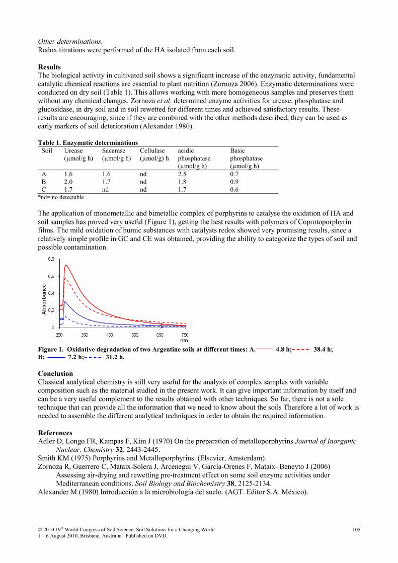
© 2010 19th World Congress of Soil Science, Soil Solutions for a Changing World
1 – 6 August 2010, Brisbane, Australia. Published on DVD. 105
Other determinations.
Redox titrations were performed of the HA isolated from each soil.
Results The biological activity in cultivated soil shows a significant increase of the enzymatic activity, fundamental
catalytic chemical reactions are essential to plant nutrition (Zornoza 2006). Enzymatic determinations were
conducted on dry soil (Table 1). This allows working with more homogeneous samples and preserves them
without any chemical changes. Zornoza et al. determined enzyme activities for urease, phosphatase and
glucosidase, in dry soil and in soil rewetted for different times and achieved satisfactory results. These
results are encouraging, since if they are combined with the other methods described, they can be used as
early markers of soil deterioration (Alexander 1980).
Table 1. Enzymatic determinations
Soil Urease
(µmol/g h)
Sacarase
(µmol/g h)
Cellulase
(µmol/g) h
acidic
phosphatase
(µmol/g h)
Basic
phosphatase
(µmol/g h)
A 1.6 1.6 nd 2.5 0.7
B 2.0 1.7 nd 1.8 0.9
C 1.7 nd nd 1.7 0.6 *nd= no detectable
The application of monometallic and bimetallic complex of porphyrins to catalyse the oxidation of HA and
soil samples has proved very useful (Figure 1), getting the best results with polymers of Coprotoporphyrin
films. The mild oxidation of humic substances with catalysts redox showed very promising results, since a
relatively simple profile in GC and CE was obtained, providing the ability to categorize the types of soil and
possible contamination.
Figure 1. Oxidative degradation of two Argentine soils at different times: A. 4.8 h; 38.4 h;
B: 7.2 h; 31.2 h.
Conclusion Classical analytical chemistry is still very useful for the analysis of complex samples with variable
composition such as the material studied in the present work. It can give important information by itself and
can be a very useful complement to the results obtained with other techniques. So far, there is not a sole
technique that can provide all the information that we need to know about the soils Therefore a lot of work is
needed to assemble the different analytical techniques in order to obtain the required information.
References Adler D, Longo FR, Kampas F, Kim J (1970) On the preparation of metalloporphyrins Journal of Inorganic
Nuclear. Chemistry 32, 2443-2445.
Smith KM (1975) Porphyrins and Metalloporphyrins. (Elsevier, Amsterdam).
Zornoza R, Guerrero C, Mataix-Solera J, Arcenegui V, García-Orenes F, Mataix- Beneyto J (2006)
Assessing air-drying and rewetting pre-treatment effect on some soil enzyme activities under
Mediterranean conditions. Soil Biology and Biochemistry 38, 2125-2134.
Alexander M (1980) Introducción a la microbiología del suelo. (AGT. Editor S.A. México).
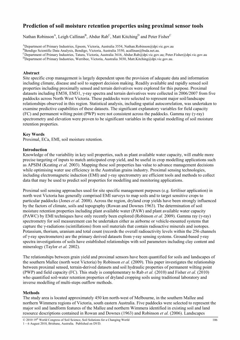
© 2010 19th World Congress of Soil Science, Soil Solutions for a Changing World
1 – 6 August 2010, Brisbane, Australia. Published on DVD. 106
Prediction of soil moisture retention properties using proximal sensor tools
Nathan RobinsonA, Leigh Callinan
B, Abdur Rab
C, Matt Kitching
D and Peter Fisher
C
ADepartment of Primary Industries, Epsom, Victoria, Australia 3554, [email protected] BBendigo Scientific Data Analysis, Bendigo, Victoria, Australia 3550, [email protected]. CDepartment of Primary Industries, Tatura, Victoria, Australia 3616, [email protected]; [email protected] DDepartment of Primary Industries, Werribee, Victoria, Australia 3030, [email protected].
Abstract Site specific crop management is largely dependent upon the provision of adequate data and information
including climate, disease and soil to support decision making. Readily available and rapidly sensed soil
properties including proximally sensed and terrain derivatives were explored for this purpose. Proximal
datasets including EM38, EM31, γ-ray spectra and terrain derivatives were collected in 2006/2007 from five
paddocks across North West Victoria. These paddocks were selected to represent major soil/landscape
relationships observed in this region. Statistical analysis, including spatial autocorrelation, was undertaken to
examine predictive capabilities of these datasets. The significant explanatory variables for field capacity
(FC) and permanent wilting point (PWP) were not consistent across the paddocks. Gamma ray (γ-ray)
spectrometry and elevation were proven to be significant variables in the spatial modelling of soil moisture
retention properties.
Key Words Proximal, ECa, EMI, soil moisture retention.
Introduction Knowledge of the variability in key soil properties, such as plant available water capacity, will enable more
precise targeting of inputs to match anticipated crop yield, and be useful in crop modelling applications such
as APSIM (Keating et al. 2003). Mapping these soil properties has value to advance management decisions
while optimising water use efficiency in the Australian grains industry. Proximal sensing technologies,
including electromagnetic induction (EMI) and γ-ray spectrometry are efficient tools and methods to collect
data that may be used to predict soil properties for modelling and monitoring applications.
Proximal soil sensing approaches used for site specific management purposes (e.g. fertiliser application) in
north west Victoria has generally comprised EMI surveys to map soils and to target sensitive crops to
particular paddocks (Jones et al. 2008). Across the region, dryland crop yields have been strongly influenced
by the factors of climate, soils and topography (Rowan and Downes 1963). The determination of soil
moisture retention properties including plant available water (PAW) and plant available water capacity
(PAWC) by EMI techniques have only recently been explored (Robinson et al. 2009). Gamma ray (γ-ray)
spectrometry for soil measurement can be undertaken either as airborne or vehicle-mounted systems that
capture the γ-radiations (scintillations) from soil materials that contain radioactive minerals and isotopes.
Potassium, thorium, uranium and total count (records the overall radioactivity levels within the 256 channels
of γ-ray spectrometers) are the primary derived datasets from γ-ray sensing systems. Ground-based γ-ray
spectra investigations of soils have established relationships with soil parameters including clay content and
mineralogy (Taylor et al. 2002).
The relationships between grain yield and proximal sensors have been quantified for soils and landscapes of
the southern Mallee (north west Victoria) by Robinson et al. (2009). This paper investigates the relationship
between proximal sensed, terrain-derived datasets and soil hydraulic properties of permanent wilting point
(PWP) and field capacity (FC). This study is complementary to Rab et al. (2010) and Fisher et al. (2010)
who quantified soil-water retention properties of dryland cropping soils using traditional laboratory and
inverse modelling of multi-steps outflow methods.
Methods The study area is located approximately 450 km north-west of Melbourne, in the southern Mallee and
northern Wimmera regions of Victoria, south eastern Australia. Five paddocks were selected to represent the
major soil and landform features of the Mallee and northern Wimmera identified in existing soil and land
resource descriptions contained in Rowan and Downes (1963) and Robinson et al. (2006). Landscapes
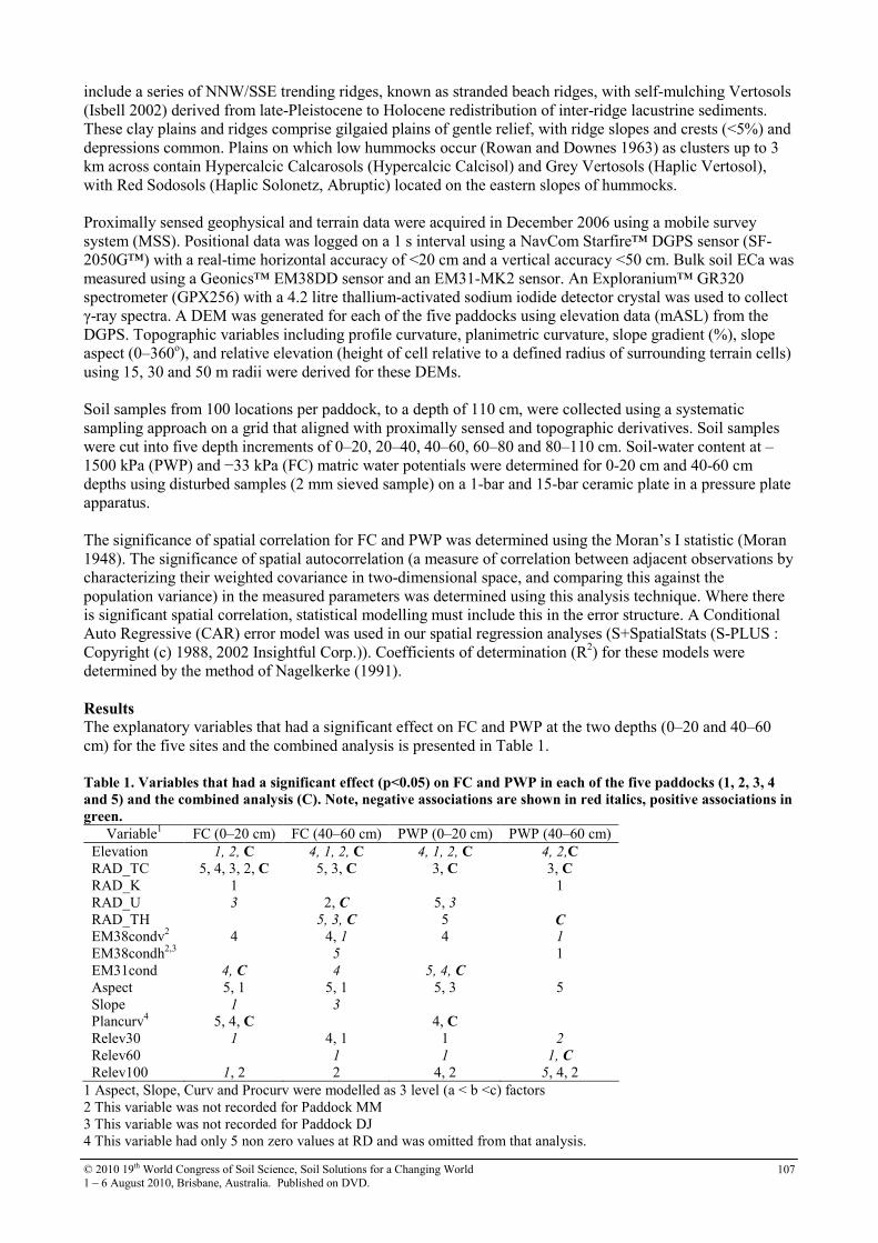
© 2010 19th World Congress of Soil Science, Soil Solutions for a Changing World
1 – 6 August 2010, Brisbane, Australia. Published on DVD. 107
include a series of NNW/SSE trending ridges, known as stranded beach ridges, with self-mulching Vertosols
(Isbell 2002) derived from late-Pleistocene to Holocene redistribution of inter-ridge lacustrine sediments.
These clay plains and ridges comprise gilgaied plains of gentle relief, with ridge slopes and crests (<5%) and
depressions common. Plains on which low hummocks occur (Rowan and Downes 1963) as clusters up to 3
km across contain Hypercalcic Calcarosols (Hypercalcic Calcisol) and Grey Vertosols (Haplic Vertosol),
with Red Sodosols (Haplic Solonetz, Abruptic) located on the eastern slopes of hummocks.
Proximally sensed geophysical and terrain data were acquired in December 2006 using a mobile survey
system (MSS). Positional data was logged on a 1 s interval using a NavCom Starfire™ DGPS sensor (SF-
2050G™) with a real-time horizontal accuracy of <20 cm and a vertical accuracy <50 cm. Bulk soil ECa was
measured using a Geonics™ EM38DD sensor and an EM31-MK2 sensor. An Exploranium™ GR320
spectrometer (GPX256) with a 4.2 litre thallium-activated sodium iodide detector crystal was used to collect
γ-ray spectra. A DEM was generated for each of the five paddocks using elevation data (mASL) from the
DGPS. Topographic variables including profile curvature, planimetric curvature, slope gradient (%), slope
aspect (0–360o), and relative elevation (height of cell relative to a defined radius of surrounding terrain cells)
using 15, 30 and 50 m radii were derived for these DEMs.
Soil samples from 100 locations per paddock, to a depth of 110 cm, were collected using a systematic
sampling approach on a grid that aligned with proximally sensed and topographic derivatives. Soil samples
were cut into five depth increments of 0–20, 20–40, 40–60, 60–80 and 80–110 cm. Soil-water content at –
1500 kPa (PWP) and −33 kPa (FC) matric water potentials were determined for 0-20 cm and 40-60 cm
depths using disturbed samples (2 mm sieved sample) on a 1-bar and 15-bar ceramic plate in a pressure plate
apparatus.
The significance of spatial correlation for FC and PWP was determined using the Moran’s I statistic (Moran
1948). The significance of spatial autocorrelation (a measure of correlation between adjacent observations by
characterizing their weighted covariance in two-dimensional space, and comparing this against the
population variance) in the measured parameters was determined using this analysis technique. Where there
is significant spatial correlation, statistical modelling must include this in the error structure. A Conditional
Auto Regressive (CAR) error model was used in our spatial regression analyses (S+SpatialStats (S-PLUS :
Copyright (c) 1988, 2002 Insightful Corp.)). Coefficients of determination (R2) for these models were
determined by the method of Nagelkerke (1991).
Results The explanatory variables that had a significant effect on FC and PWP at the two depths (0–20 and 40–60
cm) for the five sites and the combined analysis is presented in Table 1.
Table 1. Variables that had a significant effect (p<0.05) on FC and PWP in each of the five paddocks (1, 2, 3, 4
and 5) and the combined analysis (C). Note, negative associations are shown in red italics, positive associations in
green.
Variable1
FC (0–20 cm) FC (40–60 cm) PWP (0–20 cm) PWP (40–60 cm)
Elevation 1, 2, C 4, 1, 2, C 4, 1, 2, C 4, 2,C
RAD_TC 5, 4, 3, 2, C 5, 3, C 3, C 3, C
RAD_K 1 1
RAD_U 3 2, C 5, 3
RAD_TH 5, 3, C 5 C
EM38condv2
4 4, 1 4 1
EM38condh2,3
5 1
EM31cond 4, C 4 5, 4, C
Aspect 5, 1 5, 1 5, 3 5
Slope 1 3
Plancurv4
5, 4, C 4, C
Relev30 1 4, 1 1 2
Relev60 1 1 1, C
Relev100 1, 2 2 4, 2 5, 4, 2
1 Aspect, Slope, Curv and Procurv were modelled as 3 level (a < b <c) factors
2 This variable was not recorded for Paddock MM
3 This variable was not recorded for Paddock DJ
4 This variable had only 5 non zero values at RD and was omitted from that analysis.
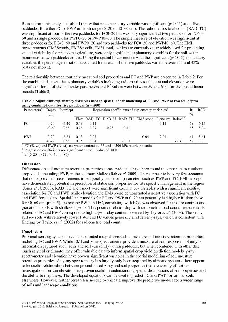
© 2010 19th World Congress of Soil Science, Soil Solutions for a Changing World
1 – 6 August 2010, Brisbane, Australia. Published on DVD. 108
Results from this analysis (Table 1) show that no explanatory variable was significant (p<0.15) at all five
paddocks, for either FC or PWP or depth range (0–20 or 40–60 cm). The radiometrics total count (RAD_TC)
was significant at four of the five paddocks for FC0–20 but was only significant at two paddocks for FC40–
60 and a single paddock for PWP0–20 or PWP40–60. The simple measure of elevation was significant at
three paddocks for FC40–60 and PWP0–20 and two paddocks for FC0–20 and PWP40–60. The EMI
measurements (EM38condv, EM38condh, EM31cond), which are currently quite widely used for predicting
spatial variability for precision agriculture, were only significant explanatory variables for the soil water
parameters at two paddocks or less. Using the spatial linear models with the significant (p<0.15) explanatory
variables the percentage variation accounted for at each of the five paddocks varied between 11 and 43%
(data not shown).
The relationship between routinely measured soil properties and FC and PWP are presented in Table 2. For
the combined data set, the explanatory variables including radiometrics total count and elevation were
significant for all of the soil water parameters and R2 values were between 59 and 61% for the spatial linear
models (Table 2).
Table 2. Significant explanatory variables used in spatial linear modelling of FC and PWP at two soil depths
using combined data for five paddocks (n = 500).
ParametersA Depth
(cm)
Intercept Regression coefficients of explanatory variablesB R
2
(%)
RSEC
Elev RAD_TC RAD_U RAD_TH EM31cond Plancurv Relev60
FC 0-20 -3.40 0.18 0.12 3.11 59 6.13
40-60 7.55 0.25 0.09 -0.23 -0.11 58 5.94
PWP 0-20 -5.83 0.13 0.07 -0.04 2.04 61 3.61
40-60 1.68 0.15 0.04 -0.07 -2.31 59 3.33 A FC (% wt) and PWP (% wt) are water content at -33 and -1500 kPa matric potentials
B Regression coefficients are significant at the P value of <0.01
C df (0-20 = 486, 40-60 = 487)
Discussion Differences in soil moisture retention properties across paddocks have been found to contribute to resultant
crop yields, including PWP, in the southern Mallee (Rab et al. 2009). There appear to be very few accounts
that relate proximal measurements to temporally stable soil parameters such as PWP and FC. EMI surveys
have demonstrated potential in prediction of stable soil properties for site specific management in the region
(Jones et al. 2008). RAD_TC and aspect were significant explanatory variables with a significant positive
association for FC and PWP while elevation and EM31cond demonstrated a negative association with FC
and PWP for all sites. Spatial linear models for FC and PWP at 0–20 cm generally had higher R2 than those
for 40–60 cm (p=0.05). Increasing PWP and FC, correlating with ECa, was observed for texture contrast and
gradational soils with shallow topsoils. This positive relationship with radiometric total count measurements
related to FC and PWP correspond to high topsoil clay content observed by Taylor et al. (2008). The sandy
surface soils with relatively lower PWP and FC values generally emit fewer γ-rays, which is consistent with
findings by Taylor et al. (2002) for radiometric total count.
Conclusion Proximal sensing systems have demonstrated a rapid approach to measure soil moisture retention properties
including FC and PWP. While EMI and γ-ray spectrometry provide a measure of soil response, not only is
information captured about soils and soil variability within paddocks, but when combined with other data
(such as yield or climate) may offer valuable data to inform spatial crop yield prediction models. γ-ray
spectrometry and elevation have proven significant variables in the spatial modelling of soil moisture
retention properties. As γ-ray spectrometry has largely only been acquired by airborne systems, there appear
to be useful relationships between ground-based γ-ray and soil properties that are worthy of further
investigation. Terrain elevation has proven useful in understanding spatial distributions of soil properties and
the ability to map these. The developed equations can be used to predict FC and PWP for similar soils
elsewhere. However, further research is needed to validate/improve the predictive models for a wider range
of soils and landscape conditions.

© 2010 19th World Congress of Soil Science, Soil Solutions for a Changing World
1 – 6 August 2010, Brisbane, Australia. Published on DVD. 109
Acknowledgement This research was jointly funded the Grains Research and Development Corporation and the Victorian
Department of Primary Industries.
References Fisher PFD, Aumann CD, Vrugt JA, Hopmans JW, Rab MA, Kitching M, Robinson NJ (2010) Rapid
estimation of soil water retention functions. In ‘19th World Congress of Soil Science, Soil Solutions for a
Changing World. 1 – 6 August 2010, Brisbane, Australia’. Published on DVD.
Isbell RF (2002) ‘The Australian Soil Classification’. Revised Edition. (CSIRO Publishing: Victoria).
Jones B, Llewellyn R, O’Leary G (2008) Sodium, chloride, clay and conductivity: consistent relationships
help to make EM surveys useful for site specific management in the Mallee. In ‘Global Issues, Paddock
Action, Proceedings of the 14th Australian Agronomy Conference’. (Australian Society of Agronomy).
Keating BA, Carberry PS, Hammer GL, Probert ME, Robertson MJ, Holzworth D, Huth NI, Hargreaves
JNG, Meinke H, Hochman Z, McLean G, Verburg K, Snow V, Dimes JP, Silburn M, Wang E, Brown S,
Bristow KL, Asseng S, Chapman S, McCown RL, Freebairn DM, Smith CJ (2003) An overview of
APSIM, a model designed for farming systems simulation. European Journal of Agronomy 18, 267-288.
Moran P (1948) The interpretation on statistical maps. Journal of the Royal Statistical Society 10, 243–251.
Rab MA, Fisher PD, Armstrong RD, Abuzar M, Robinson NJ, Chandra S (2009) Advances in precision
agriculture in south-eastern Australia. IV. Spatial variability in plant-available water capacity of soil and
its relationship with yield in site-specific management zones. Crops and Pastures 60, 885-900.
Rab MA, Fisher PD, Robinson NJ, Kitching M, Aumann CD, Imhof M, Chandra S (2010) Plant available
water capacity of dryland cropping soils in the south-eastern Australia. In ‘19th World Congress of Soil
Science, Soil Solutions for a Changing World. 1 – 6 August 2010, Brisbane, Australia’. Published on
DVD.
Robinson N, Rees D, Reynard K, Boyle G, Imhof M, Martin J, Rowan J, Smith C, Sheffield K and Giles S
(2006) ‘A land resource assessment of the Wimmera region’. (Department of Primary Industries:
Bendigo).
Robinson NJ, Rampant PC, Callinan APL, Rab MA and Fisher PD (2009) Advances in precision agriculture
in south-eastern Australia. II. Spatio-temporal prediction of crop yield using terrain derivatives and
proximally sensed data. Crops and Pastures 60, 859-869.
Rowan JN, Downes RG (1963) ‘A study of the land in north-western Victoria’. Technical Communication
No. 2. (Soil Conservation Authority: Victoria).
Taylor J, Short M, McBratney A, Wilson J (2008) Comparison of the ability of multiple soil sensors to
predict soil properties in a Scottish potato production system. In ‘Proceedings of 1st Global Workshop on
High Resolution Digital Soil Sensing & Mapping’. (Sydney, New South Wales, Australia).
Taylor MJ, Smetten K, Pracilio G, Verboom W (2002) Relationships between soil properties and high-
resolution radiometrics, central eastern weatbelt, Western Australia. Exploration Geophysics 33, 95–102.
Nagelkerke NJ (1991) A note on a general definition of the coefficient of determination. Biometrika 78, 691–
692.
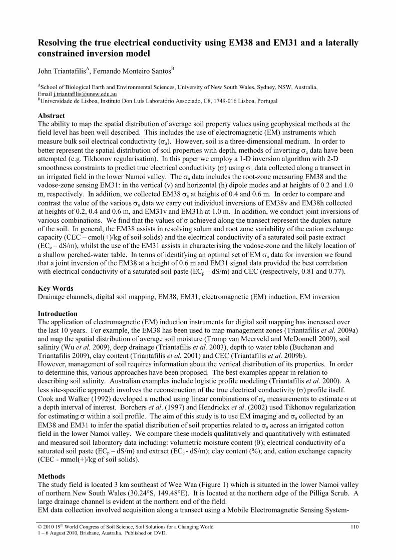
© 2010 19th World Congress of Soil Science, Soil Solutions for a Changing World
1 – 6 August 2010, Brisbane, Australia. Published on DVD. 110
Resolving the true electrical conductivity using EM38 and EM31 and a laterally
constrained inversion model
John TriantafilisA, Fernando Monteiro Santos
B
ASchool of Biological Earth and Environmental Sciences, University of New South Wales, Sydney, NSW, Australia,
Email [email protected] BUniversidade de Lisboa, Instituto Don Luís Laboratório Associado, C8, 1749-016 Lisboa, Portugal
Abstract The ability to map the spatial distribution of average soil property values using geophysical methods at the
field level has been well described. This includes the use of electromagnetic (EM) instruments which
measure bulk soil electrical conductivity (σa). However, soil is a three-dimensional medium. In order to
better represent the spatial distribution of soil properties with depth, methods of inverting σa data have been
attempted (e.g. Tikhonov regularisation). In this paper we employ a 1-D inversion algorithm with 2-D
smoothness constraints to predict true electrical conductivity (σ) using σa data collected along a transect in
an irrigated field in the lower Namoi valley. The σa data includes the root-zone measuring EM38 and the
vadose-zone sensing EM31: in the vertical (v) and horizontal (h) dipole modes and at heights of 0.2 and 1.0
m, respectively. In addition, we collected EM38 σa at heights of 0.4 and 0.6 m. In order to compare and
contrast the value of the various σa data we carry out individual inversions of EM38v and EM38h collected
at heights of 0.2, 0.4 and 0.6 m, and EM31v and EM31h at 1.0 m. In addition, we conduct joint inversions of
various combinations. We find that the values of σ achieved along the transect represent the duplex nature
of the soil. In general, the EM38 assists in resolving solum and root zone variability of the cation exchange
capacity (CEC – cmol(+)/kg of soil solids) and the electrical conductivity of a saturated soil paste extract
(ECe – dS/m), whilst the use of the EM31 assists in characterising the vadose-zone and the likely location of
a shallow perched-water table. In terms of identifying an optimal set of EM σa data for inversion we found
that a joint inversion of the EM38 at a height of 0.6 m and EM31 signal data provided the best correlation
with electrical conductivity of a saturated soil paste (ECp – dS/m) and CEC (respectively, 0.81 and 0.77).
Key Words Drainage channels, digital soil mapping, EM38, EM31, electromagnetic (EM) induction, EM inversion
Introduction The application of electromagnetic (EM) induction instruments for digital soil mapping has increased over
the last 10 years. For example, the EM38 has been used to map management zones (Triantafilis et al. 2009a)
and map the spatial distribution of average soil moisture (Tromp van Meerveld and McDonnell 2009), soil
salinity (Wu et al. 2009), deep drainage (Triantafilis et al. 2003), depth to water table (Buchanan and
Triantafilis 2009), clay content (Triantafilis et al. 2001) and CEC (Triantafilis et al. 2009b).
However, management of soil requires information about the vertical distribution of its properties. In order
to determine this, various approaches have been proposed. The best examples appear in relation to
describing soil salinity. Australian examples include logistic profile modeling (Triantafilis et al. 2000). A
less site-specific approach involves the reconstruction of the true electrical conductivity (σ) profile itself.
Cook and Walker (1992) developed a method using linear combinations of σa measurements to estimate σ at
a depth interval of interest. Borchers et al. (1997) and Hendrickx et al. (2002) used Tikhonov regularization
for estimating σ within a soil profile. The aim of this study is to use EM imaging and σa collected by an
EM38 and EM31 to infer the spatial distribution of soil properties related to σa across an irrigated cotton
field in the lower Namoi valley. We compare these models qualitatively and quantitatively with estimated
and measured soil laboratory data including: volumetric moisture content (θ); electrical conductivity of a
saturated soil paste (ECp – dS/m) and extract (ECe - dS/m); clay content (%); and, cation exchange capacity
(CEC - mmol(+)/kg of soil solids).
Methods The study field is located 3 km southeast of Wee Waa (Figure 1) which is situated in the lower Namoi valley
of northern New South Wales (30.24°S, 149.48°E). It is located at the northern edge of the Pilliga Scrub. A
large drainage channel is evident at the northern end of the field.
EM data collection involved acquisition along a transect using a Mobile Electromagnetic Sensing System-
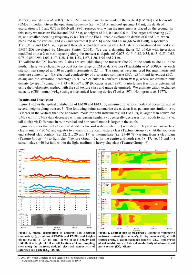
© 2010 19th World Congress of Soil Science, Soil Solutions for a Changing World
1 – 6 August 2010, Brisbane, Australia. Published on DVD. 111
MESS (Triantafilis et al. 2002). Here EM38 measurements are made in the vertical (EM38v) and horizontal
(EM38h) modes. Given the operating frequency (i.e. 14.5 kHz) and coil spacing (1.0 m), the depth of
exploration is 1.5 and 0.75 m (McNeill 1990), respectively, when the instrument is placed on the ground. In
this study we measure EM38v and EM38h σa at heights of 0.2, 0.4 and 0.6 m. The larger coil spacing (3.7
m) and smaller operating frequency (9.8 kHz) of the EM31 enable exploration depths of 6 and 3 m, when
measured in the vertical (EM31v) and horizontal (EM31h) mode and 1.0 m (McNeill 1980), respectively.
The EM38 and EM31 σa is passed through a modified version of a 1-D laterally constrained method (i.e.
EM34-2D) developed by Monteiro Santos (2004). We use a damping factor (λ) of 0.6 with inversions
modelled onto a 2 m mesh spacing along the transect at depths of: 0.075, 0.15, 0.25, 0.35, 0.45, 0.55, 0.65,
0.75, 0.85, 0.95, 1.05, 1.17, 1.28, 1.40, 1.53, 1.67, 1.80, 1.95 and 2.1 m.
To validate the EM inversions, 9 sites are available along the transect: Site 22 in the south to site 14 in the
north. These were chosen to account for the range of EM σa data values (Triantafilis et al. 2009b). At each
site soil was sampled at 0.30 m depth increments to 2.1 m. The samples were analysed for: gravimetric soil
moisture content (w - %), electrical conductivity of a saturated soil paste (ECp - dS/m) and its extract (ECe -
dS/m) and the saturation percentage (SP). We calculate θ (cm3/cm
3) from w x ρ, where we estimate bulk
density (ρ- g/cm3) using ρ = 1.73 – 0.0067 x SP (Rhoades et al. 1989). Particle size fraction is determined
using the hydrometer method with the soil texture class and grade determined. We estimate cation exchange
capacity (CEC - mmol(+)/kg) using a mechanical leaching device (Tucker 1974; Holmgren et al. 1977).
Results and Discussion
Figure 1 shows the spatial distribution of EM38 and EM31 σa measured in various modes of operation and at
several heights along transect 3. The following points summarize the σa data: i) σa patterns are similar; ii) σa
is larger in the vertical than the horizontal mode for both instruments; iii) EM31 σa is larger than equivalent
EM38 σa; iv) EM38 data decreases with increasing height: v) σa generally decreases from south to north (i.e.
tail ditch); vi) Difference in σa in vertical and horizontal mode is larger in the south.
Figure 2a shows the plot of estimated volumetric soil water content (θ) with depth. Topsoil and subsurface
clay is small (< 20 %) and equates to a loam to silty loam texture class (Texture Group - 3). At the southern
end subsoil clay content (i.e. 22, 21, 20 and 19) is intermediate (i.e. 25-40 %) varying from a clay loam
(Texture Group - 4) to light clay (Texture Group - 5). In the centre and north (i.e. 18, 17, 16, 15 and 14)
subsoil clay (> 40 %) falls within the light-medium to heavy clay class (Texture Group - 6).
Figure 1. Spatial distribution of apparent soil electrical
conductivity (σσσσa - mS/m) of EM38v and EM38h and heights
of: (a) 0.2 m, (b) 0.4 m; and, (c) 0.6 m and EM31v and
EM31h at a height of 1.0 m; (d) location of 9 soil sampling
sites along the transect; and, (e) electrical conductivity of
saturated soil paste (ECp - dS/m).
Figure 2. Contour plot of measured a) estimated volumetric
moisture content (θθθθ - cm3/cm3), b) clay content (%), c) soil
texture grade, d) cation exchange capacity (CEC - cmol(+)/kg
of soil solids), and e) electrical conductivity of saturated soil
paste extract (ECe - dS/m).
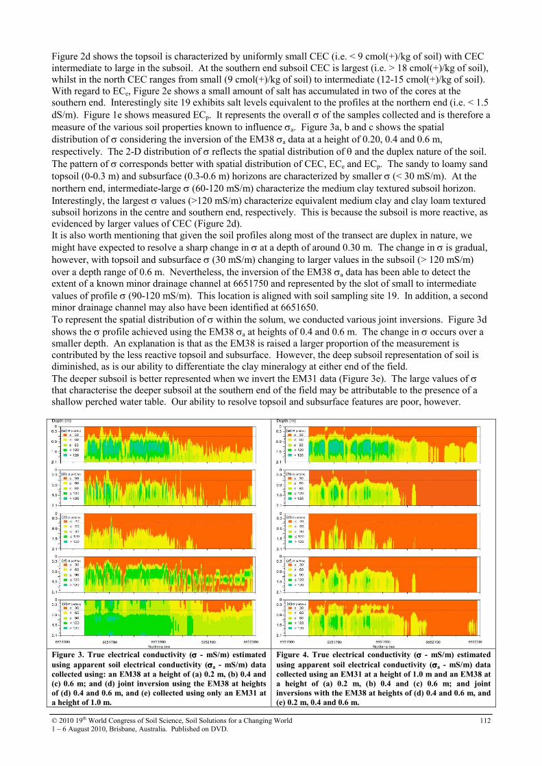
© 2010 19th World Congress of Soil Science, Soil Solutions for a Changing World
1 – 6 August 2010, Brisbane, Australia. Published on DVD. 112
Figure 2d shows the topsoil is characterized by uniformly small CEC (i.e. < 9 cmol(+)/kg of soil) with CEC
intermediate to large in the subsoil. At the southern end subsoil CEC is largest (i.e. > 18 cmol(+)/kg of soil),
whilst in the north CEC ranges from small (9 cmol(+)/kg of soil) to intermediate (12-15 cmol(+)/kg of soil).
With regard to ECe, Figure 2e shows a small amount of salt has accumulated in two of the cores at the
southern end. Interestingly site 19 exhibits salt levels equivalent to the profiles at the northern end (i.e. < 1.5
dS/m). Figure 1e shows measured ECp. It represents the overall σ of the samples collected and is therefore a
measure of the various soil properties known to influence σa. Figure 3a, b and c shows the spatial
distribution of σ considering the inversion of the EM38 σa data at a height of 0.20, 0.4 and 0.6 m,
respectively. The 2-D distribution of σ reflects the spatial distribution of θ and the duplex nature of the soil.
The pattern of σ corresponds better with spatial distribution of CEC, ECe and ECp. The sandy to loamy sand
topsoil (0-0.3 m) and subsurface (0.3-0.6 m) horizons are characterized by smaller σ (< 30 mS/m). At the
northern end, intermediate-large σ (60-120 mS/m) characterize the medium clay textured subsoil horizon.
Interestingly, the largest σ values (>120 mS/m) characterize equivalent medium clay and clay loam textured
subsoil horizons in the centre and southern end, respectively. This is because the subsoil is more reactive, as
evidenced by larger values of CEC (Figure 2d).
It is also worth mentioning that given the soil profiles along most of the transect are duplex in nature, we
might have expected to resolve a sharp change in σ at a depth of around 0.30 m. The change in σ is gradual,
however, with topsoil and subsurface σ (30 mS/m) changing to larger values in the subsoil (> 120 mS/m)
over a depth range of 0.6 m. Nevertheless, the inversion of the EM38 σa data has been able to detect the
extent of a known minor drainage channel at 6651750 and represented by the slot of small to intermediate
values of profile σ (90-120 mS/m). This location is aligned with soil sampling site 19. In addition, a second
minor drainage channel may also have been identified at 6651650.
To represent the spatial distribution of σ within the solum, we conducted various joint inversions. Figure 3d
shows the σ profile achieved using the EM38 σa at heights of 0.4 and 0.6 m. The change in σ occurs over a
smaller depth. An explanation is that as the EM38 is raised a larger proportion of the measurement is
contributed by the less reactive topsoil and subsurface. However, the deep subsoil representation of soil is
diminished, as is our ability to differentiate the clay mineralogy at either end of the field.
The deeper subsoil is better represented when we invert the EM31 data (Figure 3e). The large values of σ
that characterise the deeper subsoil at the southern end of the field may be attributable to the presence of a
shallow perched water table. Our ability to resolve topsoil and subsurface features are poor, however.
Figure 3. True electrical conductivity (σσσσ - mS/m) estimated
using apparent soil electrical conductivity (σσσσa - mS/m) data
collected using: an EM38 at a height of (a) 0.2 m, (b) 0.4 and
(c) 0.6 m; and (d) joint inversion using the EM38 at heights
of (d) 0.4 and 0.6 m, and (e) collected using only an EM31 at
a height of 1.0 m.
Figure 4. True electrical conductivity (σσσσ - mS/m) estimated
using apparent soil electrical conductivity (σσσσa - mS/m) data
collected using an EM31 at a height of 1.0 m and an EM38 at
a height of (a) 0.2 m, (b) 0.4 and (c) 0.6 m; and joint
inversions with the EM38 at heights of (d) 0.4 and 0.6 m, and
(e) 0.2 m, 0.4 and 0.6 m.
© 2010 19th World Congress of Soil Science, Soil Solutions for a Changing World
1 – 6 August 2010, Brisbane, Australia. Published on DVD. 113
The spatial distribution of σ developed from joint inversions between the EM31 and EM38 at individual
heights of 0.2, 0.4 and 0.6 m are shown in Figure 4a, 4b and 4c, respectively. Joint inversions are also shown
for various other combinations. In terms of determining an optimal set of σa data, we found that the use of the
EM38 σa at a height of 0.6 m and EM31 data (Figure 4c) led to the highest correlation with ECp (0.81).
Conclusion
The spatial distribution of topsoil, subsurface and subsoil properties are discernible by the inversion of σa
data collected along an intensively surveyed transect within an irrigated cotton growing field south-east of
Wee Waa. The root-zone model, where the EM38 σa data (EM38v and EM38h) available at heights of 0.20,
0.4 and 0.6 m discern the major soil types and physiographic features within the field. This includes: the
duplex soil profiles with more reactive clay (> 12 cmol(+)/kg) at the southern end of the field and the duplex
soil profiles associated with a prior stream at the northern end. The location of two minor drainage channels,
equivalent to the soil that characterises the northern end are discerned at the southern end.
To better resolve the duplex nature of the soil we develop a solum model, which involved passing the entire
EM38 σa data set (EM38v and EM38h) available at various heights (0.20, 0.40 and 0.60 m) through our 1-D
inversion algorithm. Whilst we are able to better represent the clear and abrupt change in clay content, the
inversion model is unable to resolve differences in subsoil σ of the two types of soil profile that characterize
the northern and southern end of the field. The use of the EM31 σa data in reconstructing σ in the root-zone
appears to be limited. Its greatest contribution is in characterizing and defining the lower boundary. This
conclusion is borne out when we developed two joint EM inversion models of the soil and vadose-zone (e.g.
developed by entering the EM38v and EM38h σa data available at various heights. Statistical analysis
showed that the best correlation with ECp (0.81) is achievable by jointly inverting the EM38 σa at a height of
0.60 m with the EM31 σa data. The approach we have used has been applied to the joint inversion of EM38
and EM34 σa data (Triantafilis and Santos 2009) as well as to a DUALEM-421 (Monteiro Santos et al.
2009).
References Borchers B, Uram T, Hendrickx JMH (1997). Tikhonov regularization of electrical conductivity depth profiles in field soils. Soil Science
Society of America Journal 61, 1004-1009.
Buchanan SM, Triantafilis, J (2009) Mapping water table depth using geophysical and environmental variables. Ground Water 47, 80-96.
Cook PG, Walker GR (1992) Depth profiles of electrical conductivity from linear combinations of electromagnetic induction measurements.
Soil Science Society of America Journal 56, 1015-1022.
Hendrickx JMH, Borchers B, Corwin DL, Lesch SM, Hilgendorf AC, Schlue J (2002). Inversion of soil conductivity profiles from
electromagnetic induction measurements: Theory and experimental verification. Soil Science Society of America Journal 66, 673-685.
Holmgren GGS, Juve RL, Geschwender RC (1977) A mechanically controlled variable leaching device. Soil Science Society of America
Journal 41, 1207-1208.
McNeill JD (1980) Electromagnetic terrain conductivity measurements at low induction numbers. Technical note TN-6, Geonics Limited,
Mississauga Ontario, Canada.
McNeill JD (1990) Geonics EM38 Ground Conductivity Meter: EM38 Operating Manual. Geonics Limited, Mississauga Ontario, Canada.
Monteiro Santos FA (2004) 1-D laterally constrained inversion of EM34 profiling data. Journal of Applied Geophysics 56, 123-134.
Rhoades JD, Manteghi NA, Shouse PJ, and Alves WJ 1989 Soil electrical conductivity and soil salinity: New formulations and calibrations.
Soil Science Society of America Journal 53, 433–439.
Monteiro Santos FA, Triantafilis J, Bruzgulis, KE, Roe JAE (2010). Inversion of DUALEM-421 profiling data using a 1-D laterally
constrained algorithm. Vadose Zone Journal 9, 117-125.
Tucker BM (1974) Laboratory procedure for cation exchange measurements in soils. CSIRO Division of Soils, Technical Paper No 23.
(CSIRO, Australia).
Triantafilis J, Monteiro Santos FA (2009). 2-dimensional soil and vadose zone representation using an EM38 and EM34 and a laterally
constrained inversion model. Australian Journal of Soil Research 47, 809-920.
Triantafilis J, Laslett GM, McBratney AB (2000) Calibrating an electromagnetic induction instrument to measure salinity in soil under
irrigated cotton. Soil Science Society of America Journal 64, 1009-1017.
Triantafilis J, Huckel AI, Odeh IOA (2001) Comparison of statistical prediction methods for estimating field-scale clay content using
different combinations of ancillary variables. Soil Science 166, 415-427.
Triantafilis J, Ahmed MF, Odeh IOA (2002) Application of a mobile electromagnetic sensing system (MESS) to assess cause and
management of soil salinisation in an irrigated cotton-growing field. Soil Use Management 18, 330-339.
Triantafilis J, Huckel AI, Odeh IOA (2003) Field-scale assessment of deep drainage risk. Irrigation Science 21, 183-192.
Triantafilis J, Kerridge B, Buchanan SM (2009a) Digital soil-class mapping from proximal and remotely sensed data at the field level.
Agronomy Journal 101, 841-853.
Triantafilis J, Lau KL, Buchanan SM (2009b). Field level digital soil mapping of cation exchange capacity using electromagnetic induction
and a hierarchical spatial regression model in the lower Namoi Valley, Australia. Australian Journal of Soil Research 47, 651-663.
Tromp-van Meerveld J, McDonnell JJ (2009) Assessment of multi-frequency electromagnetic induction for determining soil moisture
patterns at the hillslope scale. Journal of Hydrology 368, 56-67.
Tucker BM (1974) Laboratory procedure for cation exchange measurements in soils. CSIRO Australia, Division of Soils. Technical Paper
No. 23. CSIRO, Australia.
Wu YK, Yang JS, Li XM (2009) Study on spatial variability of soil salinity based on spectral indices and EM38 readings. Spectroscopy and
Spectral Analysis 29, 1023-1027.
© 2010 19th World Congress of Soil Science, Soil Solutions for a Changing World
1 – 6 August 2010, Brisbane, Australia. Published on DVD. 114
Simultaneous determination of chromium species by ion chromatography
coupled with inductively coupled plasma mass spectrometry Girish Choppala
A,B, Mohammad Mahmudur Rahman
A,B, Zuliang Chen
A,B Nanthi Bolan
A,B and Megharaj
MallavarapuA,B
ACRC-Contamination Assessment and Remediation of Environment (CRC CARE), Mawson Lakes, SA-5095. BCERAR, University of South Australia, Mawson Lakes, SA-5095, Email [email protected]
Abstract Huge amounts of chromium (Cr) compounds are releasing into the environment because of anthropogenic
activities. Speciation of chromium compounds is important in understanding the toxicity because of
contrasting characters of hexavalent (Cr(VI) and trivalent Cr(III) chromium). An improved method for
estimation of Cr species in environmental samples is developed using different complexing ligands and
detected by ion chromatography (IC) coupled with inductively coupled plasma- mass spectrometer (ICP-
MS). Among six complexing ligands probed, NTA 3Na+ and HEDTA gave the highest UV response and
highest selectivity for Cr(III) complexation using an Agilent anion-exchange column with a mobile phase
containing 20 mM NH4NO3 at pH 7.1 without Cl- interference. Conditions including pH, concentration ratio
[Cr(III) / NTA 3Na+, HEDTA)] and stability of Cr(III) complexes were investigated with pre-column
derivatization. In conclusion, the proposed method could be used for the quantification of chromium species
in contaminated water and soils within minutes.
Key Words Chromium toxicity, speciation, ligands, complexation, retention time, IC-ICP MS.
Introduction Chromium is used in many industries including electroplating, timber treatment, tannery industries, iron and
steel industries (Nriagu and Pacyna 1988). As a result, anthropogenic discharge of chromium (Cr) often
occurs into the environment. The toxicity, mobility and bioavailability of Cr depend on its oxidation state. Cr
species exist in different oxidation states, from Cr2+
to Cr6+
. However, trivalent (Cr3+
) and hexavalent (Cr6+
)
are predominant species in environment. Hexavalent chromium (Cr(VI)) species present as chromate (CrO42-
),
bichromate (HCrO4-
) and dichromate (Cr2O72-
) which are toxic and mutagenic, mobile in alkaline and
slightly acidic soils (Venitt and Levy 1974; Bauthio 1992). Nevertheless, Cr3+
is relatively non toxic and is
considered as an essential nutrient at low levels in the human diet for effective glucose maintenance
(Anderson 1989). Trivalent chromium [Cr(III)] mostly retained onto soil particles and also precipitated as
Cr(III) hydroxide (Bolan et al. 2003).
Quantification of total chromium in environmental samples may not be sufficient to understand the
distribution of various Cr species because of contrasting properties of Cr(III) and Cr(VI). Detailed
information about oxidation states is essential to understand the toxicity of Cr. Therefore estimation of
Cr(VI) and Cr(III) separately, rather than as total Cr is crucial. Several methodologies are available to
measure Cr species in environmental samples using atomic absorption spectrometry (AAS) (Subramanian
1988; Sperling et al. 1992; James et al. 1995 and Adria-Cerezo et al. 2000). Ion chromatography (IC)
coupled to inductively coupled plasma- mass spectrometry (ICP-MS) is currently available for metal
speciation. However, the simultaneous determination of Cr(VI) and Cr(III) using a single chromatography
column is difficult because Cr(III) is in the cationic form, however Cr(VI) is anionic . Hence, conversion of
cationic Cr(III) to anionic form and subsequent separation of these two anionic species with a single anion-
exchange chromatography hyphened with ICP-MS is possible since ICP-MS provides an ultra-sensitive
elemental detector.
For separation of Cr(III) and Cr(VI) species, liquid chromatography (LC) coupled with inductively coupled
plasma (ICP-MS) has been developed (Camara et al. 2000; Michalke 2002). Normally simultaneous
determination of chromium is difficult because separation of Cr(VI) and Cr(III) using a single anionic
column is impossible. However this problem can be resolved using two approaches. The first of these
approaches uses an anion-exchange column and a cation-exchange guard column in series or a mixed mode
column to retain both species (Pantsar-Kallio et al. 1996; Barnowski et al. 1997). The second approach
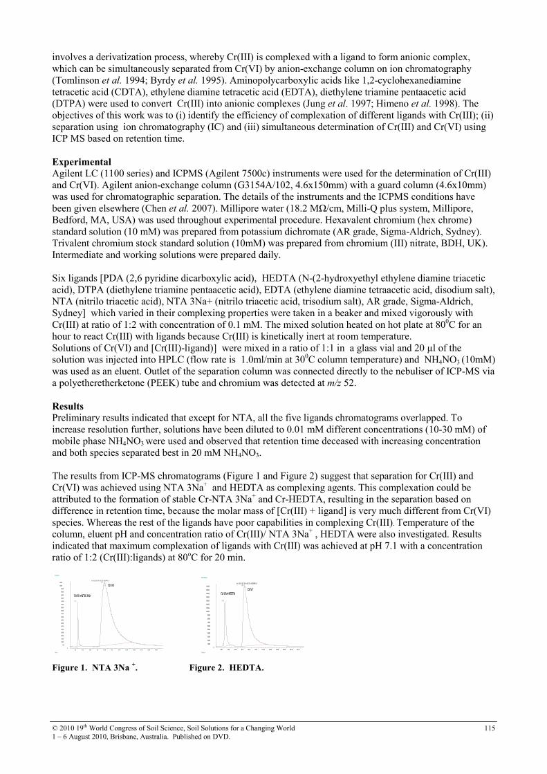
© 2010 19th World Congress of Soil Science, Soil Solutions for a Changing World
1 – 6 August 2010, Brisbane, Australia. Published on DVD. 115
involves a derivatization process, whereby Cr(III) is complexed with a ligand to form anionic complex,
which can be simultaneously separated from Cr(VI) by anion-exchange column on ion chromatography
(Tomlinson et al. 1994; Byrdy et al. 1995). Aminopolycarboxylic acids like 1,2-cyclohexanediamine
tetracetic acid (CDTA), ethylene diamine tetracetic acid (EDTA), diethylene triamine pentaacetic acid
(DTPA) were used to convert Cr(III) into anionic complexes (Jung et al. 1997; Himeno et al. 1998). The
objectives of this work was to (i) identify the efficiency of complexation of different ligands with Cr(III); (ii)
separation using ion chromatography (IC) and (iii) simultaneous determination of Cr(III) and Cr(VI) using
ICP MS based on retention time.
Experimental Agilent LC (1100 series) and ICPMS (Agilent 7500c) instruments were used for the determination of Cr(III)
and Cr(VI). Agilent anion-exchange column (G3154A/102, 4.6x150mm) with a guard column (4.6x10mm)
was used for chromatographic separation. The details of the instruments and the ICPMS conditions have
been given elsewhere (Chen et al. 2007). Millipore water (18.2 MΩ/cm, Milli-Q plus system, Millipore,
Bedford, MA, USA) was used throughout experimental procedure. Hexavalent chromium (hex chrome)
standard solution (10 mM) was prepared from potassium dichromate (AR grade, Sigma-Aldrich, Sydney).
Trivalent chromium stock standard solution (10mM) was prepared from chromium (III) nitrate, BDH, UK).
Intermediate and working solutions were prepared daily.
Six ligands [PDA (2,6 pyridine dicarboxylic acid), HEDTA (N-(2-hydroxyethyl ethylene diamine triacetic
acid), DTPA (diethylene triamine pentaacetic acid), EDTA (ethylene diamine tetraacetic acid, disodium salt),
NTA (nitrilo triacetic acid), NTA 3Na+ (nitrilo triacetic acid, trisodium salt), AR grade, Sigma-Aldrich,
Sydney] which varied in their complexing properties were taken in a beaker and mixed vigorously with
Cr(III) at ratio of 1:2 with concentration of 0.1 mM. The mixed solution heated on hot plate at 800C for an
hour to react Cr(III) with ligands because Cr(III) is kinetically inert at room temperature.
Solutions of Cr(VI) and [Cr(III)-ligand)] were mixed in a ratio of 1:1 in a glass vial and 20 µl of the
solution was injected into HPLC (flow rate is 1.0ml/min at 300C column temperature) and NH4NO3 (10mM)
was used as an eluent. Outlet of the separation column was connected directly to the nebuliser of ICP-MS via
a polyetheretherketone (PEEK) tube and chromium was detected at m/z 52.
Results Preliminary results indicated that except for NTA, all the five ligands chromatograms overlapped. To
increase resolution further, solutions have been diluted to 0.01 mM different concentrations (10-30 mM) of
mobile phase NH4NO3 were used and observed that retention time deceased with increasing concentration
and both species separated best in 20 mM NH4NO3.
The results from ICP-MS chromatograms (Figure 1 and Figure 2) suggest that separation for Cr(III) and
Cr(VI) was achieved using NTA 3Na+ and HEDTA as complexing agents. This complexation could be
attributed to the formation of stable Cr-NTA 3Na+ and Cr-HEDTA, resulting in the separation based on
difference in retention time, because the molar mass of [Cr(III) + ligand] is very much different from Cr(VI)
species. Whereas the rest of the ligands have poor capabilities in complexing Cr(III). Temperature of the
column, eluent pH and concentration ratio of Cr(III)/ NTA 3Na+ , HEDTA were also investigated. Results
indicated that maximum complexation of ligands with Cr(III) was achieved at pH 7.1 with a concentration
ratio of 1:2 (Cr(III):ligands) at 80oC for 20 min.
2.00 4.00 6.00 8.00 10.00 12.00 14.00 16.00 18.00 20.00 22.00 24.00 0
5000
10000
15000
20000
25000
30000
35000
40000
45000
50000
55000
60000
65000
70000
75000
80000
85000
90000
95000
100000
105000
Time-->
Abundance
Ion 52.00 (51.70 to 52 .70): 001SMPL.D
2.02
9.27
Cr(III)+NTA 3Na+
Cr(VI)
2.00 4.00 6.00 8.00 10.00 12.00 14.00 16.00 18.00 20.00 22.00 24.000
10000
20000
30000
40000
50000
60000
70000
80000
90000
100000
110000
120000
130000
140000
150000
160000
170000
Time-->
Abundance
Ion 52.00 (51.70 to 52.70): 003SMPL.D
2.42
7.98
Cr(III)+HEDTA Cr(VI)
Figure 1. NTA 3Na
+. Figure 2. HEDTA.
© 2010 19th World Congress of Soil Science, Soil Solutions for a Changing World
1 – 6 August 2010, Brisbane, Australia. Published on DVD. 116
Conclusions The results suggest that stable chromium-chelate complexes, [Cr(III) – NTA] and [Cr(III) – HEDTA] were
formed and successfully separated for both Cr(III) and Cr(VI) by complexing ligands based on difference in
retention times on IC-ICP MS. This method could be used as a basis for separation and simultaneous
quantification of Cr(III) and Cr(VI) in water and soil solutions. Further study is required to determine the
stability constants of Cr(III) – NTA] and [Cr(III) – HEDTA] complexes.
References Adria-Cerezo DM, Llobat-Estellés M, Maurí-Aucejo AR (2000) Preconcentration and speciation of
chromium in waters using solid-phase extraction and atomic absorption spectrometry. Talanta 51, 531-
536.
Anderson R (1989) Essentiality of chromium in humans. Sci Total Environment 86, 75-81.
Bauthio F (1992) Toxic effects of chromium and its compounds. Biological trace element research 32, 145-
153.
Bolan N, Adriano D, Natesan R, Koo BJ (2003) Effects of organic amendments on the reduction and
phytoavailability of chromate in mineral soil. Journal of Environmental Quality 32, 120-128.
Cámara C, Cornelis R, Quevauviller P (2000) Assessment of methods currently used for the determination of
Cr and Se species in solutions. Trends in Analytical Chemistry 19, 189-194.
Chen ZL, Megharaj M and Naidu R (2007) Speciation of chromium in waste water using ion
chromatography inductively coupled plasma mass spectrometry. Talanta 72, 394-400.
Himeno S, Nakashima Y, Sano K (1998) Simultaneous determination of chromium (VI) and chromium (III)
by capillary electrophoresis. Analytical Science 14, 369-373.
Inoue Y, Sakai T, Kumagai H (1995) Simultaneous determination of chromium (III) and chromium (VI) by
ion chromatography with inductively coupled plasma mass spectrometry. Journal of chromatography A
706, 127-136.
James BR, Petura JC, Vitale RJ, Mussoline GR (1995) Hexavalent chromium extraction from soils: a
comparison of five methods. Environmental science and technology 29, 2377-2381.
Jung GY, Kim YS, Lim HB (1997) Simultaneous Determination of Chromium (III) and Chromium (VI) in
Aqueous Solution by Capillary Electrophoresis with On-Column UV-VIS Detection. Analytical Sciences
13, 463-467.
Nriagu JO, Pacyna JM (1988) Quantitative assessment of worldwide contamination of air, water and soils by
trace metals, Nature 33, 134-139.
Sarzanini C and Bruzzoniti MC (2001) Metal species determination by ion chromatography. Trends in
Analytical Chemistry 20, 304-310.
Semenova OP, Timerbaev AR, Gagstadter R, Bonn GK (2005) Speciation of chromium ions by capillary
zone electrophoresis. Journal of High Resolution Chromatography 19, 177-179.
Sperling M, Xu S, Welz B (1992) Determination of chromium (III) and chromium (VI) in water using flow
injection on-line Preconcentration with selective adsorption on activated alumina and flame atomic
absorption spectrometric detection. Analytical Chemistry 64, 3101-3108.
Subramanian KS (1988) Determination of chromium (III) and chromium (VI) by ammonium
pyrrolidinecarbodithioate-methyl isobutyl ketone furnace atomic absorption spectrometry. Analytical
chemistry (Washington, DC) 60, 11-15.
Venitt S, Levy LS (1974) Mutagenicity of chromates in bacteria and its relevance to chromate
carcinogenesis. Nature 250, 493-495.
Weckhuysen BM, Wachs IE, Schoonheydt RA (1996) Surface chemistry and spectroscopy of chromium in
inorganic oxides. Chemical reviews 96, 3327-3350.
Weiss J (1995) ‘Ion chromatography, 2nd
edition’. (VCH Weinheim).
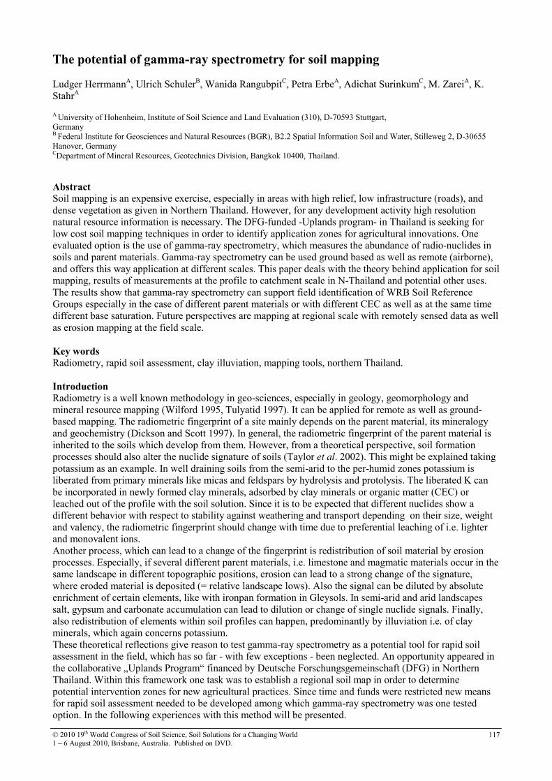
© 2010 19th World Congress of Soil Science, Soil Solutions for a Changing World
1 – 6 August 2010, Brisbane, Australia. Published on DVD. 117
The potential of gamma-ray spectrometry for soil mapping
Ludger HerrmannA, Ulrich Schuler
B, Wanida Rangubpit
C, Petra Erbe
A, Adichat Surinkum
C, M. Zarei
A, K.
StahrA
A University of Hohenheim, Institute of Soil Science and Land Evaluation (310), D-70593 Stuttgart,
Germany
B Federal Institute for Geosciences and Natural Resources (BGR), B2.2 Spatial Information Soil and Water, Stilleweg 2, D-30655
Hanover, Germany CDepartment of Mineral Resources, Geotechnics Division, Bangkok 10400, Thailand.
Abstract Soil mapping is an expensive exercise, especially in areas with high relief, low infrastructure (roads), and
dense vegetation as given in Northern Thailand. However, for any development activity high resolution
natural resource information is necessary. The DFG-funded -Uplands program- in Thailand is seeking for
low cost soil mapping techniques in order to identify application zones for agricultural innovations. One
evaluated option is the use of gamma-ray spectrometry, which measures the abundance of radio-nuclides in
soils and parent materials. Gamma-ray spectrometry can be used ground based as well as remote (airborne),
and offers this way application at different scales. This paper deals with the theory behind application for soil
mapping, results of measurements at the profile to catchment scale in N-Thailand and potential other uses.
The results show that gamma-ray spectrometry can support field identification of WRB Soil Reference
Groups especially in the case of different parent materials or with different CEC as well as at the same time
different base saturation. Future perspectives are mapping at regional scale with remotely sensed data as well
as erosion mapping at the field scale.
Key words Radiometry, rapid soil assessment, clay illuviation, mapping tools, northern Thailand.
Introduction Radiometry is a well known methodology in geo-sciences, especially in geology, geomorphology and
mineral resource mapping (Wilford 1995, Tulyatid 1997). It can be applied for remote as well as ground-
based mapping. The radiometric fingerprint of a site mainly depends on the parent material, its mineralogy
and geochemistry (Dickson and Scott 1997). In general, the radiometric fingerprint of the parent material is
inherited to the soils which develop from them. However, from a theoretical perspective, soil formation
processes should also alter the nuclide signature of soils (Taylor et al. 2002). This might be explained taking
potassium as an example. In well draining soils from the semi-arid to the per-humid zones potassium is
liberated from primary minerals like micas and feldspars by hydrolysis and protolysis. The liberated K can
be incorporated in newly formed clay minerals, adsorbed by clay minerals or organic matter (CEC) or
leached out of the profile with the soil solution. Since it is to be expected that different nuclides show a
different behavior with respect to stability against weathering and transport depending on their size, weight
and valency, the radiometric fingerprint should change with time due to preferential leaching of i.e. lighter
and monovalent ions.
Another process, which can lead to a change of the fingerprint is redistribution of soil material by erosion
processes. Especially, if several different parent materials, i.e. limestone and magmatic materials occur in the
same landscape in different topographic positions, erosion can lead to a strong change of the signature,
where eroded material is deposited (= relative landscape lows). Also the signal can be diluted by absolute
enrichment of certain elements, like with ironpan formation in Gleysols. In semi-arid and arid landscapes
salt, gypsum and carbonate accumulation can lead to dilution or change of single nuclide signals. Finally,
also redistribution of elements within soil profiles can happen, predominantly by illuviation i.e. of clay
minerals, which again concerns potassium.
These theoretical reflections give reason to test gamma-ray spectrometry as a potential tool for rapid soil
assessment in the field, which has so far - with few exceptions - been neglected. An opportunity appeared in
the collaborative „Uplands Program“ financed by Deutsche Forschungsgemeinschaft (DFG) in Northern
Thailand. Within this framework one task was to establish a regional soil map in order to determine
potential intervention zones for new agricultural practices. Since time and funds were restricted new means
for rapid soil assessment needed to be developed among which gamma-ray spectrometry was one tested
option. In the following experiences with this method will be presented.
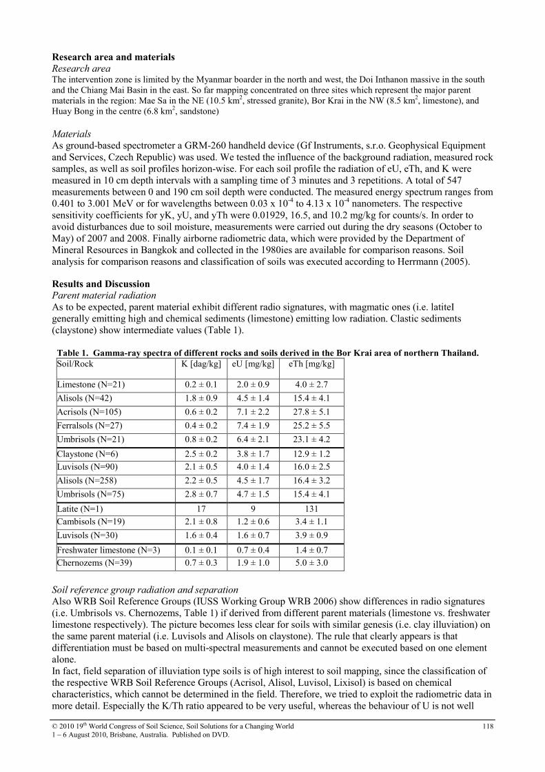
© 2010 19th World Congress of Soil Science, Soil Solutions for a Changing World
1 – 6 August 2010, Brisbane, Australia. Published on DVD. 118
Research area and materials Research area The intervention zone is limited by the Myanmar boarder in the north and west, the Doi Inthanon massive in the south
and the Chiang Mai Basin in the east. So far mapping concentrated on three sites which represent the major parent
materials in the region: Mae Sa in the NE (10.5 km2, stressed granite), Bor Krai in the NW (8.5 km
2, limestone), and
Huay Bong in the centre (6.8 km2, sandstone)
Materials
As ground-based spectrometer a GRM-260 handheld device (Gf Instruments, s.r.o. Geophysical Equipment
and Services, Czech Republic) was used. We tested the influence of the background radiation, measured rock
samples, as well as soil profiles horizon-wise. For each soil profile the radiation of eU, eTh, and K were
measured in 10 cm depth intervals with a sampling time of 3 minutes and 3 repetitions. A total of 547
measurements between 0 and 190 cm soil depth were conducted. The measured energy spectrum ranges from
0.401 to 3.001 MeV or for wavelengths between 0.03 x 10⁻⁴
to 4.13 x 10⁻⁴
nanometers. The respective
sensitivity coefficients for yK, yU, and yTh were 0.01929, 16.5, and 10.2 mg/kg for counts/s. In order to
avoid disturbances due to soil moisture, measurements were carried out during the dry seasons (October to
May) of 2007 and 2008. Finally airborne radiometric data, which were provided by the Department of
Mineral Resources in Bangkok and collected in the 1980ies are available for comparison reasons. Soil
analysis for comparison reasons and classification of soils was executed according to Herrmann (2005).
Results and Discussion Parent material radiation
As to be expected, parent material exhibit different radio signatures, with magmatic ones (i.e. latiteI
generally emitting high and chemical sediments (limestone) emitting low radiation. Clastic sediments
(claystone) show intermediate values (Table 1).
Table 1. Gamma-ray spectra of different rocks and soils derived in the Bor Krai area of northern Thailand.
Soil/Rock K [dag/kg] eU [mg/kg] eTh [mg/kg]
Limestone (N=21) 0.2 ± 0.1 2.0 ± 0.9 4.0 ± 2.7
Alisols (N=42) 1.8 ± 0.9 4.5 ± 1.4 15.4 ± 4.1
Acrisols (N=105) 0.6 ± 0.2 7.1 ± 2.2 27.8 ± 5.1
Ferralsols (N=27) 0.4 ± 0.2 7.4 ± 1.9 25.2 ± 5.5
Umbrisols (N=21) 0.8 ± 0.2 6.4 ± 2.1 23.1 ± 4.2
Claystone (N=6) 2.5 ± 0.2 3.8 ± 1.7 12.9 ± 1.2
Luvisols (N=90) 2.1 ± 0.5 4.0 ± 1.4 16.0 ± 2.5
Alisols (N=258) 2.2 ± 0.5 4.5 ± 1.7 16.4 ± 3.2
Umbrisols (N=75) 2.8 ± 0.7 4.7 ± 1.5 15.4 ± 4.1
Latite (N=1) 17 9 131
Cambisols (N=19) 2.1 ± 0.8 1.2 ± 0.6 3.4 ± 1.1
Luvisols (N=30) 1.6 ± 0.4 1.6 ± 0.7 3.9 ± 0.9
Freshwater limestone (N=3) 0.1 ± 0.1 0.7 ± 0.4 1.4 ± 0.7
Chernozems (N=39) 0.7 ± 0.3 1.9 ± 1.0 5.0 ± 3.0
Soil reference group radiation and separation
Also WRB Soil Reference Groups (IUSS Working Group WRB 2006) show differences in radio signatures
(i.e. Umbrisols vs. Chernozems, Table 1) if derived from different parent materials (limestone vs. freshwater
limestone respectively). The picture becomes less clear for soils with similar genesis (i.e. clay illuviation) on
the same parent material (i.e. Luvisols and Alisols on claystone). The rule that clearly appears is that
differentiation must be based on multi-spectral measurements and cannot be executed based on one element
alone.
In fact, field separation of illuviation type soils is of high interest to soil mapping, since the classification of
the respective WRB Soil Reference Groups (Acrisol, Alisol, Luvisol, Lixisol) is based on chemical
characteristics, which cannot be determined in the field. Therefore, we tried to exploit the radiometric data in
more detail. Especially the K/Th ratio appeared to be very useful, whereas the behaviour of U is not well
© 2010 19th World Congress of Soil Science, Soil Solutions for a Changing World
1 – 6 August 2010, Brisbane, Australia. Published on DVD. 119
understood. The latter might be a general methodological problem using the 214 Bi nuclide for uranium
estimation, since volatile radon occurs in the decay chain, which leads to a potential high estimation error.
Figure 1 shows that it is possible to nearly completely separate Alisols and Acrisols in the limestone
catchment based on radiometric data. For the cases where the separation does not work out, also results of
chemical analysis are close to the threshold values of the WRB classification (24cmolc+/kg clay, 50 % base
saturation), and the distance to the threshold values is within the detection error of the analytical method.
Figure 1. Binary plot of K and Th radiation of soil horizons from different WRB Soil Reference Groups for the
limestone catchment Bor Krai
Behaviour of K, Th, and U nuclides during soil genesis in the Bor Krai limestone catchment in N-Thailand
Limestone, due to its high carbonate concentration, exhibits overall low radiation for the measured radio nuclides.
During weathering carbonate is lost and clastic components are relatively enriched. This leads to an increasing radiation
by an increasing concentration of radio-nuclides (Figure 2). The residual of limestone after dissolution of carbonate is a
clay-rich clastic sediment, as it can also be found in the Bor Krai area. Under the given climatic conditions (seasonal
tropical, semi-arid to sub-humid), clay illuviation is the dominant soil formation process, accompanied by base loss.
Base loss by leaching leads to an absolute loss of elements including radio nuclides, which seems to affect
predominantly K. Base loss is always accompanied by silica loss, which favours the formation of two-layer clay
minerals with low substitution of central atoms and low cation exchange capacity. Consequently, total binding capacity
for cationic nuclides is constantly reducing.
Apart from absolute loss, the radio signature is depending on redistribution within the soil profile by vertical particle
movement, which mainly concerns finer particles (clay illuviation). Further on, erosion processes influence the surface
signal at erosion sites (in case of illuviation type profiles through loss of depleted topsoil material) and the whole profile
signal on depositional sites (depending on the origin of deposited material, which is in most cases topsoil material, as
shown for Umbrisols).
Though also an absolute loss for U and Th nuclides must be suspected, our measurements show an increasing signal
during terrestrial soil development, which we attribute to relative enrichment in sesquioxide components. However, this
hypothesis will need further investigation.
Figure 2. Conceptual model of radio nuclide behaviour during soil formation in the Bor Krai catchment in N-
Thailand

© 2010 19th World Congress of Soil Science, Soil Solutions for a Changing World
1 – 6 August 2010, Brisbane, Australia. Published on DVD. 120
Outlook Apart from field scale mapping, gamma-ray spectrometry has also a potential for upscaling of results and
mapping at the regional scale. Since airborne data are available for the whole of northern Thailand (Tulyatid
& Ra-Nguppits 2004), the next step will be to correlate ground-based and airborne data and to search for the
best upscaling algorithms, to connect the two scales. For potential mapping approaches which may integrate
radiometric data see Schuler (2008) and Schuler et al. (this volume). Since erosion influences the topsoil
radio signal, also erosion mapping is a potential, which is presently evaluated (see Erbe et al. this volume).
Conclusions Ground-based gamma-ray spectrometry has a potential as tool for WRB Soil Reference Group distinction at
the profile, field and (sub-)catchment scale. For illuviation type soils this is especially true if parent material
differs or CEC and base saturation are significantly different. The measurements at profile scale are of
special interest since they can replace high cost and time consuming chemical analyses (CEC and base
saturation). Therefore, this potential should be further researched in other environments (parent materials,
climates).
Further applications may concern in future erosion mapping at the field scale and regional soil and terrain
mapping if airborne data are accessible (Tulyatid & Ra-Nguppits 2004, Wilford 1995).
Acknowledgements This research was carried out within the framework of the Special Research Program 564 (“The Uplands
Program”, funded by Deutsche Forschungsgemeinschaft (DFG), whose support is gratefully acknowledged.
References Dickson BL, Scott KM (1997) Interpretation of aerial gamma-ray survey – adding the geochemical factors.
AGSO Journal of Australian Geology and Geophysics 17(2), 187-200.
Herrmann L (2005) Das kleine Bodenkochbuch (Version 2005). Institute of Soil Science and Land
Evaluation. University of Hohenheim, Stuttgart.
IUSS Working Group WRB (2006) World reference base for soil resources 2006. World Soil Resources
Reports No.103. FAO, Rome.
Schuler U (2008) Towards regionalisation of soils in northern Thailand and consequences for mapping
approaches and upscaling procedures. Hohenheimer Bodenkundliche Hefte 89, 308p.
Taylor MJ, Smettem KRJ, Pracilio G, Verboom WH (2002) Relationships between soil properties and high-
resolution radiometrics, central eastern wheatbelt, Western Australia. Exploration Geophys. 33, 95-
102.
Tuljatid J (1997) Application of airborne geophysical data to the study of Cenozoic basins in central
Thailand. PhD Thesis. School of Earth Sciences, University of Leeds, UK, 325 p.
Tuljatid J, Ra-Nguppits W (2004) Airborne geophysical data and its application on surface mapping and land
management. In ‘Innovative techniques in soil survey’ (Eds H Eswaran et al.) pp. 75- 86. (Land
Development Department, Bangkok, Thailand).
Wilford JR (1995) Airborne gamma-ray spectrometry as a tool for assessing relative landscape activity
and weathering development of regolith, including soils. AGSO Research Newsletter 22, 12-14.
© 2010 19th World Congress of Soil Science, Soil Solutions for a Changing World
1 – 6 August 2010, Brisbane, Australia. Published on DVD. 121
Three proximal sensors for mapping skeletal soils in vineyards S.Priori
A, E. Martini
B and E. A. C.Costantini
A
AC.R.A.-A.B.P., Research Center of Agrobiology and Pedology, Firenze, Italy, Email [email protected] BUniversity of Turin, Earth Science Department, Turin, Italy.
Abstract Proximal sensors are becoming widely used in precision viticulture, due to the quick, easy and non-invasive
identification of soil spatial variability. The apparent soil electrical conductivity (ECa) is the main parameter
measured by sensors, which is correlated to many factors, like soil water content, salinity, clay content and
mineralogy, bulk density, and porosity. In the last three decades, many proximal sensors for the measurement
of the ECa have been produced and commercialized. This study compares three different sensors to delineate
soil boundaries and estimate clay and skeleton content in a vineyard of the Chianti region (Central Italy). The
sensors were a geoelectric system (ARP-Automatic Resistivity Profiling) with 3 different depths of
investigation (50 cm, 100 cm and 170 cm), a single-frequency Electro-Magnetic Induction sensor (EMI,
Geonics EM38-DD), in horizontal (EM38_HDP) and vertical dipole configuration (EM38_VDP) and a
multi-frequency EMI sensor (GSSI Profiler EMP- 400), in horizontal (Profiler_HDP) and vertical
(Profiler_VDP) dipole configuration. All three sensors produced ECa maps with similar pattern. The
strongest correlations between the instruments were between ARP-50 and EM38_HDP (r = 0.774), ARP-170
and EM38_VDP (r = 0.805), and ARP-170 and Profiler in all the configurations (r = from 0.758 to 0.783).
The correlations between ECa and clay content calculated on the fine earth were low or not significant with
EM38 and Profiler (r = 0.36 to 0.61), both in vertical and horizontal configuration, and stronger with ARP (r
= 0.61 to 0.81). The correlation improved and resulted significant for all the sensors (r = 0.56 to 0.86) when
the percentage value of clay was referred to the whole soil (fine earth + skeleton).
Key Words EM38, ARP, Profiler, EMI sensors, apparent electrical conductivity, precision viticulture.
Introduction In the last years, some important farms have adopted precision viticulture (Proffitt et al. 2006) and utilize
GPS, GIS, remote sensing, soil monitoring technologies etc. To manage the spatial variability inside the
vineyard, the farmer needs geo-referenced maps, displaying areas with similar soil behavior, like hydraulic
permeability, water retention, soil fertility, etc. A rapid, non-invasive and relatively cheap mapping of the
soil apparent electric conductivity (ECa) can be a very useful tool for identifying important soil map units
and soil properties, in particular, clay (Morari et al. 2009), water content (Davies 2004; Tromp-van Meerveld
and McDonnell 2009), bulk density, and salinity (Doolittle et al. 2001). The goal of this work was to test the
suitability of three different proximal sensors in a difficult environment, as it is a vineyard on skeletal soils,
and to relate the measured ECa with the clay content.
Methods The sensors used for this work were: i) a single-frequency Electro-Magnetic Induction sensor (EMI, Geonics
EM38-DD), ii) a multi-frequency EMI sensor (GSSI Profiler EMP- 400) and iii) a geoelectric system (ARP-
Automatic Resistivity Profiling). The EM38-DD is an EMI sensor composed by two EM38 sensors, coupled
in perpendicular position (Figure 1a). Each sensor has an intercoil spacing of 1 m and operates at a frequency
of 14,600 Hz. The depths of the magnetic field penetration are about 0.75 m and 1.5 m, respectively for the
horizontal (HDP) and vertical (VDP) dipoles modes (Geonics Limited 1998). The instruments sensitivity
varies as a non-linear function of depth (McNeil 1990). The GSSI Profiler EMP-400 (Figure 1b) is a
multifrequency EMI sensor, which can operate to measure simultaneously up to 3 frequencies between 1,000
Hz and 16,000 Hz, with intercoil spacing of 1.2 m. For this study we operated at 8, 10 and 15 kHz. The
instrument can be used in vertical dipole mode (VDP) or in horizontal dipole mode (HDP), but the
instruments sensitivity in function of depth is not still studied. The output of both the EM38-DD and Profiler
is the apparent electric conductivity (ECa), measured in mS/m.
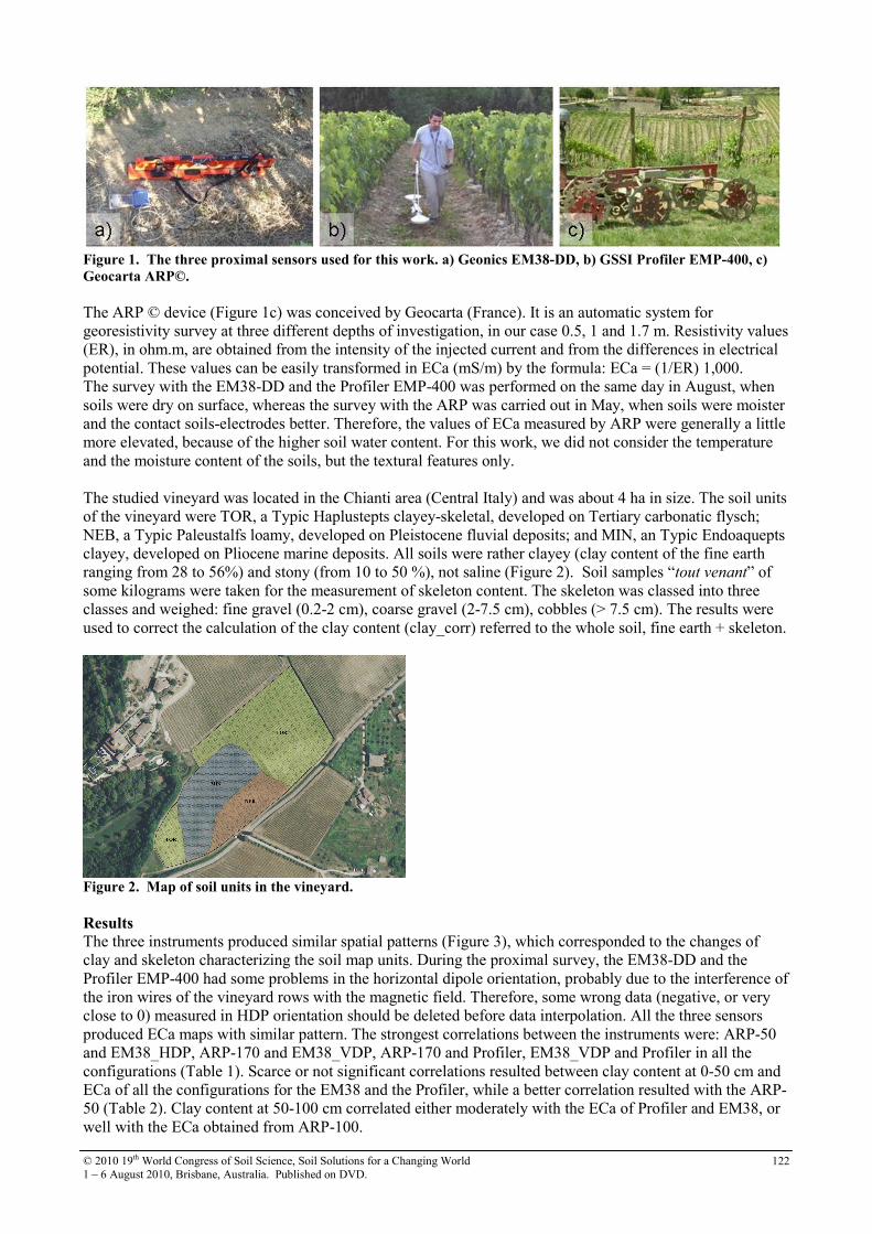
© 2010 19th World Congress of Soil Science, Soil Solutions for a Changing World
1 – 6 August 2010, Brisbane, Australia. Published on DVD. 122
Figure 1. The three proximal sensors used for this work. a) Geonics EM38-DD, b) GSSI Profiler EMP-400, c)
Geocarta ARP©.
The ARP © device (Figure 1c) was conceived by Geocarta (France). It is an automatic system for
georesistivity survey at three different depths of investigation, in our case 0.5, 1 and 1.7 m. Resistivity values
(ER), in ohm.m, are obtained from the intensity of the injected current and from the differences in electrical
potential. These values can be easily transformed in ECa (mS/m) by the formula: ECa = (1/ER) 1,000.
The survey with the EM38-DD and the Profiler EMP-400 was performed on the same day in August, when
soils were dry on surface, whereas the survey with the ARP was carried out in May, when soils were moister
and the contact soils-electrodes better. Therefore, the values of ECa measured by ARP were generally a little
more elevated, because of the higher soil water content. For this work, we did not consider the temperature
and the moisture content of the soils, but the textural features only.
The studied vineyard was located in the Chianti area (Central Italy) and was about 4 ha in size. The soil units
of the vineyard were TOR, a Typic Haplustepts clayey-skeletal, developed on Tertiary carbonatic flysch;
NEB, a Typic Paleustalfs loamy, developed on Pleistocene fluvial deposits; and MIN, an Typic Endoaquepts
clayey, developed on Pliocene marine deposits. All soils were rather clayey (clay content of the fine earth
ranging from 28 to 56%) and stony (from 10 to 50 %), not saline (Figure 2). Soil samples “tout venant” of
some kilograms were taken for the measurement of skeleton content. The skeleton was classed into three
classes and weighed: fine gravel (0.2-2 cm), coarse gravel (2-7.5 cm), cobbles (> 7.5 cm). The results were
used to correct the calculation of the clay content (clay_corr) referred to the whole soil, fine earth + skeleton.
Figure 2. Map of soil units in the vineyard.
Results The three instruments produced similar spatial patterns (Figure 3), which corresponded to the changes of
clay and skeleton characterizing the soil map units. During the proximal survey, the EM38-DD and the
Profiler EMP-400 had some problems in the horizontal dipole orientation, probably due to the interference of
the iron wires of the vineyard rows with the magnetic field. Therefore, some wrong data (negative, or very
close to 0) measured in HDP orientation should be deleted before data interpolation. All the three sensors
produced ECa maps with similar pattern. The strongest correlations between the instruments were: ARP-50
and EM38_HDP, ARP-170 and EM38_VDP, ARP-170 and Profiler, EM38_VDP and Profiler in all the
configurations (Table 1). Scarce or not significant correlations resulted between clay content at 0-50 cm and
ECa of all the configurations for the EM38 and the Profiler, while a better correlation resulted with the ARP-
50 (Table 2). Clay content at 50-100 cm correlated either moderately with the ECa of Profiler and EM38, or
well with the ECa obtained from ARP-100.
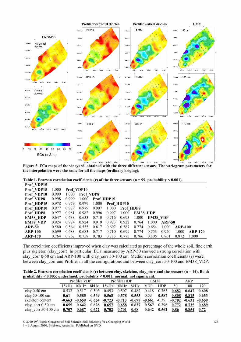
© 2010 19th World Congress of Soil Science, Soil Solutions for a Changing World
1 – 6 August 2010, Brisbane, Australia. Published on DVD. 123
Figure 3. ECa maps of the vineyard, obtained with the three different sensors. The variogram parameters for
the interpolation were the same for all the maps (ordinary kriging).
Table 1. Pearson correlation coefficients (r) of the three sensors (n = 99, probability < 0.001).
Prof_VDP15
Prof_VDP15 1.000 Prof_VDP10
Prof_VDP10 0.999 1.000 Prof_VDP8
Prof_VDP8 0.998 0.999 1.000 Prof_HDP15
Prof_HDP15 0.978 0.979 0.979 1.000 Prof_HDP10
Prof_HDP10 0.977 0.979 0.979 0.997 1.000 Prof_HDP8
Prof_HDP8 0.977 0.981 0.982 0.996 0.997 1.000 EM38_HDP
EM38_HDP 0.647 0.638 0.633 0.710 0.716 0.693 1.000 EM38_VDP
EM38_VDP 0.924 0.924 0.924 0.919 0.923 0.922 0.764 1.000 ARP-50
ARP-50 0.580 0.564 0.555 0.617 0.607 0.587 0.774 0.654 1.000 ARP-100
ARP-100 0.699 0.688 0.683 0.717 0.710 0.699 0.774 0.753 0.920 1.000 ARP-170
ARP-170 0.764 0.762 0.758 0.783 0.783 0.775 0.766 0.805 0.801 0.872 1.000
The correlation coefficients improved when clay was calculated as percentage of the whole soil, fine earth
plus skeleton (clay_corr). In particular, ECa measured by ARP-50 showed a strong correlation with
clay_corr 0-50 cm and ARP-100 with clay_corr 50-100 cm. Medium correlation coefficients (r) were
between clay_corr and Profiler in all the configurations and between clay_corr 50-100 and EM38_VDP.
Table 2. Pearson correlation coefficients (r) between clay, skeleton, clay_corr and the sensors (n = 14). Bold:
probability < 0.005; underlined: probability < 0.001; normal: not significant.
Profiler VDP Profiler HDP EM38 ARP
15kHz 10kHz 8kHz 15kHz 10kHz 8kHz VDP HDP 50 100 170
clay 0-50 cm 0.532 0.517 0.503 0.493 0.507 0.482 0.418 0.363 0.682 0.647 0.608 clay 50-100 cm 0.61 0.585 0.569 0.568 0.578 0.553 0.53 0.587 0.808 0.815 0.653 skeleton content -0.663 -0.659 -0.654 -0.723 -0.713 -0.697 -0.661 -0.39 -0.702 -0.631 -0.659 clay_corr 0-50 cm 0.655 0.642 0.628 0.657 0.658 0.637 0.567 0.396 0.772 0.735 0.689 clay_corr 50-100 cm 0.707 0.687 0.672 0.702 0.701 0.68 0.642 0.562 0.86 0.854 0.72

© 2010 19th World Congress of Soil Science, Soil Solutions for a Changing World
1 – 6 August 2010, Brisbane, Australia. Published on DVD. 124
Conclusion The patterns obtained with ECa of the three sensors were similar. The instruments could provide for a rapid,
non invasive and relatively cheap soil survey in a difficult environment, like that of a vineyard on stony soils,
although the iron wires of the rows interfered with the magnetic fields of the EMI sensors in the horizontal
dipoles configuration. The cumulative response of Profiler does not seem change at different frequencies and
was very similar to the EM38_VDP response. On top of that, both sensors were strongly correlated with
ARP-170, except for EM38_HDP, which was better correlated with ARP-50 and ARP-100.
The correlation between ECa measured by sensors and clay content was higher with the ARP system. On the
other hand, the correlation with ECa and clay_corr was strong for all sensors, except for EM38_HDP. The
proximal survey made by any of these instruments can allow to map and spatialize data of clay or clay
corrected for the skeleton content (clay_corr) with negligible errors.
Acknowledgements The authors are grateful to Annamaria Castrignanò, Donatello Sollitto and Daniela De Benedetto (CRA-
SCA, Bari, Italy) for the loan, the advices and the assistance with the EM38-DD, as well as to the SO.IN.G
and the Geostudi Astier (Livorno) for the loan and the collaboration with the ARP and the Profiler EMP-400,
respectively. A special thank is for the farm “Barone Ricasoli s.p.a.”, Gaiole in Chianti, Siena (Italy) for the
economic support of the research and for granting the access to its vineyards.
References Davies R (2004) Mapping soil properties for irrigation development in the Riverland of South Australia
using EM38. In ‘SuperSoil 2004, 3d Australian and New Zeland Soils Conference, 5-9 December 2004,
University of Sydney, Australia’. published on CD_ROM.
http://www.regional.org.au/au/asssi/supersoil2004/s5/oral.
Doolittle J, Petersen M, Wheeler T (2001) Comaprison of two electromagnetic induction tools in salinity
appraisals. Journal of Soil and Water Conservation 56, 257-262.
Geonics Limited (1998) EM38 ground conductivity meter operating manual. Mississangua, Ontario, Canada.
www.geonics.com
McNeil JD (1990) ‘Geonics EM38 Ground Conductivity Meter: EM38 Operating Manual’. (Geonics
Limited: Ontario, Canada).
Morari F, Castrignanò A, Pagliarin C.(2009) Application of multivariate geostatistics in delineating
management zones within a gravelly vineyard using geo-electrical sensors. Computers and Electroncis
in Agricolture 68, 97-107.
Proffit T, Bramley R, Lamb D, Winter E (2006) ‘Precision Viticulture’.
http://www.pvaustralia.com.au/book.html
Tromp-van Meerveld HJ, McDonnell JJ (2009) Assessment of multi-frequency electromagnetic induction for
determining soil moisture patterns at hillslope scale. Journal of Hydrology 368, 56-67.

© 2010 19th World Congress of Soil Science, Soil Solutions for a Changing World
1 – 6 August 2010, Brisbane, Australia. Published on DVD. 125
Ubiquitous Monitoring of Agricultural Fields in Asia using Sensor Network
Masaru Mizoguchi A, Tetsu Ito
B and Shoichi Mitsuishi
C
A Graduate School of Agricultural and Life Sciences, The University of Tokyo, Japan, Email [email protected] B X-Ability Ltd., Tokyo, Japan, Email [email protected] C AINEX, Ltd., Tokyo, Japan, Email [email protected]
Abstract The introduction of ubiquitous computing technology in agriculture will allow the creation of a new
agricultural system. To this end, a Japanese group has developed a number of new technologies over the past
decade. One new technology is the “Field Server”. However, as a result of our long-term monitoring trials,
some unexpected problems with the Field Server are now emerging. Here we describe the most significant
points in the use of the Field Server based on our experiences in a rainfed paddy field in Thailand, and
propose a new hybrid monitoring system incorporating a field network adapter that offers promise for safe
agricultural production management in Asia.
Key Words Field server, hybrid monitoring system, data logger, ubiquitous computing, sensor network.
Introduction The Field Server is an automatic monitoring system consisting of a CPU (a Web server), an analog-to-digital
converter, an Ethernet controller; sensors to measure air temperature, relative humidity, solar radiation, soil
moisture, soil temperature, and electrical conductivity; and a CCD camera. It can transfer high-resolution
pictures of fields and sensing data through Wi-Fi broadband networks (NARO, 2009). However, the Field
server does not have a data logging function because it is designed to be used on the network. Therefore, we
need to build a data logging system on the network in order to use the Field Server. So far, however, there
has been little research on long-term monitoring in the field by the Field Server. We have installed Field
Servers across Asia in fields of paddy rice, spinach, cabbage, and peanut since 2006 (Mizoguchi, 2008). Here
we describe some unexpected problems in the use of the Field Server which were revealed by our long-term
monitoring trials in a rainfed paddy field in Thailand. Then we propose a new hybrid monitoring system
which is improved based on our experiences and show example data obtained with the new system.
Methods Experimental site
We installed a Field Server on 2006 December 25 (Figure 1), three more on 2007 December 24, and another
on 2008 December 26 in a rainfed field in Khon Kaen, northeast Thailand (16o27.657 N, 102
o 32.443 E).
The Field Servers are at most 700 m apart. With these Field Servers, we have been monitoring
meteorological conditions (air temperature, humidity, radiation, wind velocity, precipitation) and soil
information via soil sensors (moisture content, temperature, electrical conductivity), and collecting images of
the site.
Figure 1. Field Server installed on 2007 December 24 (left) and Insect nest built on CPU board of Field
Server(right).
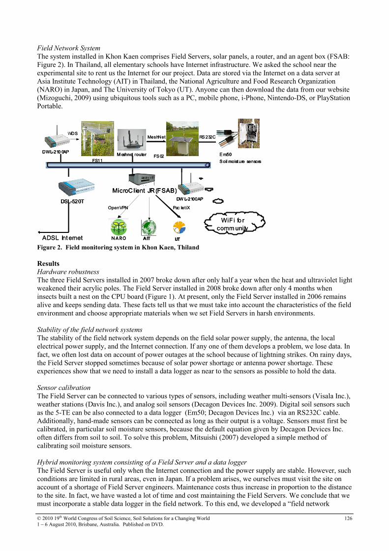
© 2010 19th World Congress of Soil Science, Soil Solutions for a Changing World
1 – 6 August 2010, Brisbane, Australia. Published on DVD. 126
Field Network System
The system installed in Khon Kaen comprises Field Servers, solar panels, a router, and an agent box (FSAB:
Figure 2). In Thailand, all elementary schools have Internet infrastructure. We asked the school near the
experimental site to rent us the Internet for our project. Data are stored via the Internet on a data server at
Asia Institute Technology (AIT) in Thailand, the National Agriculture and Food Research Organization
(NARO) in Japan, and The University of Tokyo (UT). Anyone can then download the data from our website
(Mizoguchi, 2009) using ubiquitous tools such as a PC, mobile phone, i-Phone, Nintendo-DS, or PlayStation
Portable.
RS 232C
E m50
S oil moisture sensors
M eshnet router
AIT
OpenVPN
DW L-2100AP
WiFi fo r
comm unity
MicroC lient JR (FSAB)
DSL-520T
ADSL Int ernet
Pac ket iX
UT
MeshNet
FS 02FS11
DWL-210 0AP
WDSRS 232C
E m50
S oil moisture sensors
E m50
S oil moisture sensors
M eshnet routerM eshnet router
AITAIT
OpenVPN
DW L-2100APDW L-2100AP
WiFi fo r
comm unity
MicroC lient JR (FSAB)MicroC lient JR (FSAB)
DSL-520TDSL-520T
ADSL Int ernet
Pac ket iX
UTUT
MeshNet
FS 02FS11
DWL-210 0APDWL-210 0AP
WDS
Figure 2. Field monitoring system in Khon Kaen, Thiland
Results Hardware robustness
The three Field Servers installed in 2007 broke down after only half a year when the heat and ultraviolet light
weakened their acrylic poles. The Field Server installed in 2008 broke down after only 4 months when
insects built a nest on the CPU board (Figure 1). At present, only the Field Server installed in 2006 remains
alive and keeps sending data. These facts tell us that we must take into account the characteristics of the field
environment and choose appropriate materials when we set Field Servers in harsh environments.
Stability of the field network systems
The stability of the field network system depends on the field solar power supply, the antenna, the local
electrical power supply, and the Internet connection. If any one of them develops a problem, we lose data. In
fact, we often lost data on account of power outages at the school because of lightning strikes. On rainy days,
the Field Server stopped sometimes because of solar power shortage or antenna power shortage. These
experiences show that we need to install a data logger as near to the sensors as possible to hold the data.
Sensor calibration
The Field Server can be connected to various types of sensors, including weather multi-sensors (Visala Inc.),
weather stations (Davis Inc.), and analog soil sensors (Decagon Devices Inc. 2009). Digital soil sensors such
as the 5-TE can be also connected to a data logger (Em50; Decagon Devices Inc.) via an RS232C cable.
Additionally, hand-made sensors can be connected as long as their output is a voltage. Sensors must first be
calibrated, in particular soil moisture sensors, because the default equation given by Decagon Devices Inc.
often differs from soil to soil. To solve this problem, Mitsuishi (2007) developed a simple method of
calibrating soil moisture sensors.
Hybrid monitoring system consisting of a Field Server and a data logger
The Field Server is useful only when the Internet connection and the power supply are stable. However, such
conditions are limited in rural areas, even in Japan. If a problem arises, we ourselves must visit the site on
account of a shortage of Field Server engineers. Maintenance costs thus increase in proportion to the distance
to the site. In fact, we have wasted a lot of time and cost maintaining the Field Servers. We conclude that we
must incorporate a stable data logger in the field network. To this end, we developed a “field network
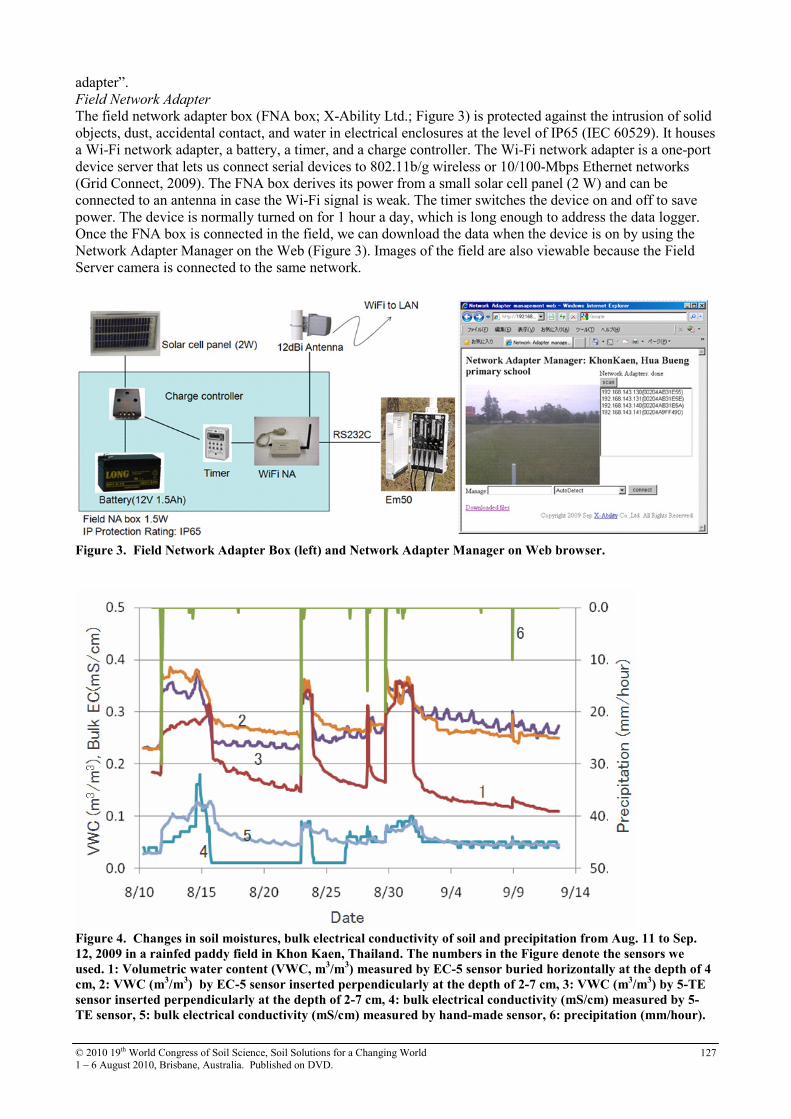
© 2010 19th World Congress of Soil Science, Soil Solutions for a Changing World
1 – 6 August 2010, Brisbane, Australia. Published on DVD. 127
adapter”.
Field Network Adapter
The field network adapter box (FNA box; X-Ability Ltd.; Figure 3) is protected against the intrusion of solid
objects, dust, accidental contact, and water in electrical enclosures at the level of IP65 (IEC 60529). It houses
a Wi-Fi network adapter, a battery, a timer, and a charge controller. The Wi-Fi network adapter is a one-port
device server that lets us connect serial devices to 802.11b/g wireless or 10/100-Mbps Ethernet networks
(Grid Connect, 2009). The FNA box derives its power from a small solar cell panel (2 W) and can be
connected to an antenna in case the Wi-Fi signal is weak. The timer switches the device on and off to save
power. The device is normally turned on for 1 hour a day, which is long enough to address the data logger.
Once the FNA box is connected in the field, we can download the data when the device is on by using the
Network Adapter Manager on the Web (Figure 3). Images of the field are also viewable because the Field
Server camera is connected to the same network.
Figure 3. Field Network Adapter Box (left) and Network Adapter Manager on Web browser.
Figure 4. Changes in soil moistures, bulk electrical conductivity of soil and precipitation from Aug. 11 to Sep.
12, 2009 in a rainfed paddy field in Khon Kaen, Thailand. The numbers in the Figure denote the sensors we
used. 1: Volumetric water content (VWC, m3/m
3) measured by EC-5 sensor buried horizontally at the depth of 4
cm, 2: VWC (m3/m
3) by EC-5 sensor inserted perpendicularly at the depth of 2-7 cm, 3: VWC (m
3/m
3) by 5-TE
sensor inserted perpendicularly at the depth of 2-7 cm, 4: bulk electrical conductivity (mS/cm) measured by 5-
TE sensor, 5: bulk electrical conductivity (mS/cm) measured by hand-made sensor, 6: precipitation (mm/hour).

© 2010 19th World Congress of Soil Science, Soil Solutions for a Changing World
1 – 6 August 2010, Brisbane, Australia. Published on DVD. 128
Downloaded data - soil moisture, bulk EC and precipitation
Figure 4 shows an example of data downloaded from an Em50 data logger, showing changes in soil
moisture, bulk electrical conductivity, and precipitation from 2009 August 11 to September 12 in the rainfed
paddy field at Khon Kaen. The numbers in the Figure denote the sensors we used. Soil moisture is measured
with two EC-5 sensors and a 5-TE sensor (Decagon Devices Inc.); A EC-5 sensor (1) is buried horizontally
at depths of 4 cm, and the other EC-5 sensor (2) and the 5-TE sensor (3) are inserted perpendicularly at the
depth of 2-7 cm. Bulk electrical conductivity is measured with a 5-TE sensor (4) and a hand-made sensor (5)
of a pair of stainless steel rods inserted perpendicularly to a depth of 20 cm. Precipitation (6) is measured
with an ECRN-50 rain gauge (Decagon Devices Inc.). Soil moisture and bulk electrical conductivity
increased after rain. The horizontal soil sensor (1), measuring at a single depth, is more sensitive that the
perpendicular ones (2, 3), which detects the average soil moisture over 2-7 cm.
Conclusion A hybrid monitoring system consisting of a Field Server and a data logger connected by a field network
adapter offers promise for safe agricultural production management in Asia. Although we have just started to
test the system, stable and easy access to the data logger is reducing the worries that we felt before.
However, there remain fundamental risks such as electric power outage and network disconnection.
Consequently, we urgently need to train field network engineers to maintain the field monitoring system. In
addition, we need to develop a more ubiquitous system based on the mobile phone system that is dependent
on existing an Internet connection. Concern about the safety of imported food is increasing in Japan and a
trial has started to show consumers a safe spinach field in Thailand (Honda, et. al, 2008). We hope that our
new field monitoring system will help to bolster consumer confidence in food that is imported from other
Asian countries into Japan.
Acknowledgement This work was partially supported by the "Data Integration & Analysis System" in the National Key
Technology (2006-2009), Ministry of Education, Culture, Sports, Science and Technology, and a Grant-in-
Aid for Scientific Research (B), 18380140 (2006-2009) by the Japan Society for the Promotion of Science.
References Davis Inc (2010) http://www.davisnet.com/
Decagon Devices (2009) Soil moisture. http://www.decagon.com/.
Fukatsu T, Hirafuji M, Kiura T (2006) Agent System for operating web-based sensor nodes via the internet.
J. Rob. Mechatron 18, 186-194.
Grid Connect (2009) http://www.gridconnect.com/wi232.html
Honda K, Shrestha A, Chinnachodteeranun R, Mizoguchi M, Shimamura H, Kameoka T (2008) Spinach
Field Monitoring for Bridging Thai Producer and Japanese Consumer under Sensor Asia. Proceeding of
SICE Annual Conference, The University Electro-Communications, Japan, pp.2582-2585
Masaru M, Shoichi M, Tetsu I, Kazuo O, Seishi N, Masayuki H, Tokihiro F, Takuji K, Kei T, Hitoshi T,
Hiromasa H, Kiyoshi H (2008) Real-time monitoring of soil information in agricultural fields in Asia
using Field server. Proceedings of 1st Global workshop on High Resolution Digital Soil Sensing and
Mapping, Vol.2, Sydney, Australia, pp.19-24
Mitsuishi S, Mizoguchi M (2007) Effects of Dry Bulk Density and Soil Type on Soil Moisture Measurement
using ECH2O-TE Probe. The ASA-CSSA-SSSA International Annual Meetings, http://a-c-
s.confex.com/crops/2007am/techprogram/P36281.HTM
Mizoguchi M (2009) Real-time Monitoring of Agricultural Field using Field Server - A project of auto-
collecting soil information from world-wide farmlands - . http://www.iai.ga.a.u-
tokyo.ac.jp/mizo/research/fieldinfomatics/
NARO (2007) Database-Model cooperation system project. http://www.agmodel.net/DataModel/ (in
Japanese)
NARO (2009) IT-AG national project. http://model.job.affrc.go.jp/FieldServer/default.htm
Visala (2010) http://www.vaisala.com/
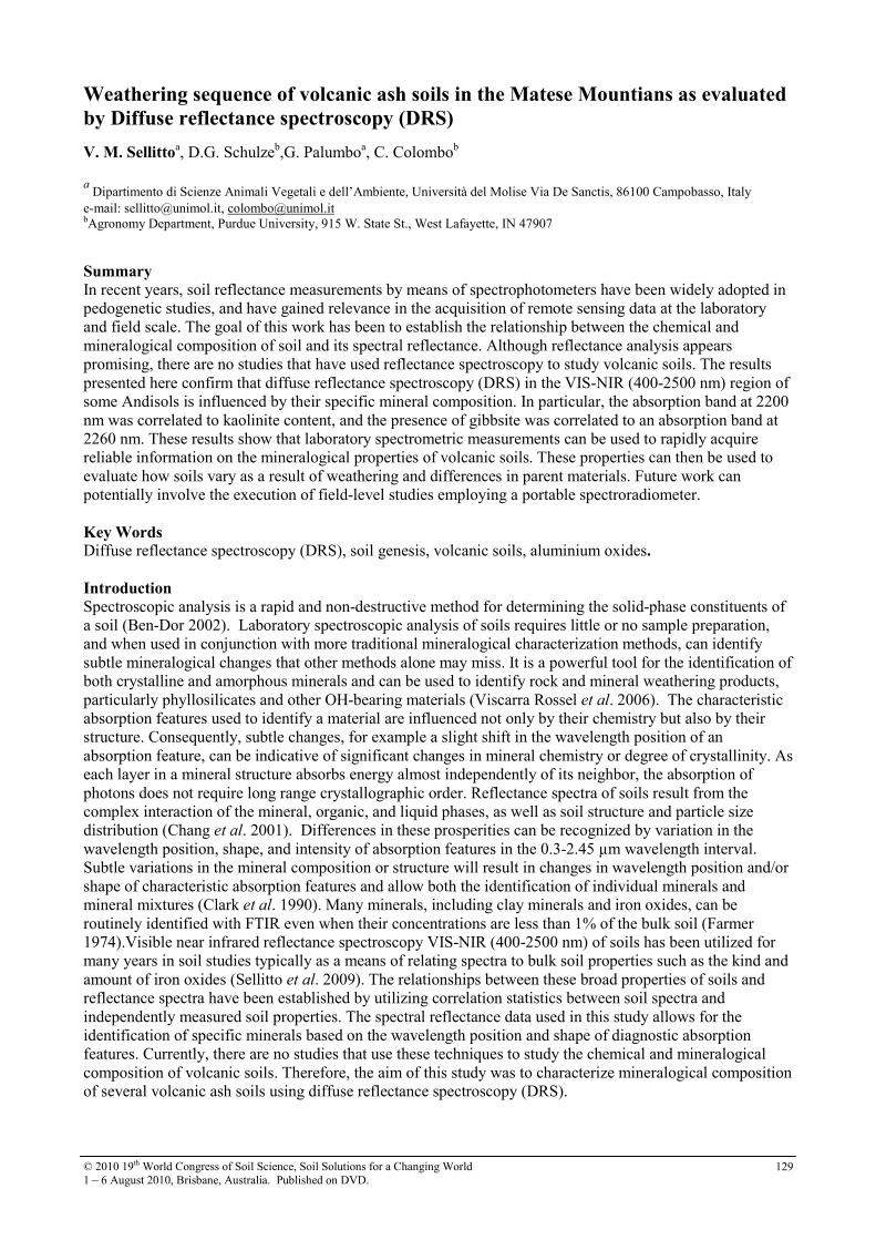
© 2010 19th World Congress of Soil Science, Soil Solutions for a Changing World
1 – 6 August 2010, Brisbane, Australia. Published on DVD. 129
Weathering sequence of volcanic ash soils in the Matese Mountians as evaluated
by Diffuse reflectance spectroscopy (DRS)
V. M. Sellittoa, D.G. Schulze
b,G. Palumbo
a, C. Colombo
b
a Dipartimento di Scienze Animali Vegetali e dell’Ambiente, Università del Molise Via De Sanctis, 86100 Campobasso, Italy
e-mail: [email protected], [email protected] bAgronomy Department, Purdue University, 915 W. State St., West Lafayette, IN 47907
Summary In recent years, soil reflectance measurements by means of spectrophotometers have been widely adopted in
pedogenetic studies, and have gained relevance in the acquisition of remote sensing data at the laboratory
and field scale. The goal of this work has been to establish the relationship between the chemical and
mineralogical composition of soil and its spectral reflectance. Although reflectance analysis appears
promising, there are no studies that have used reflectance spectroscopy to study volcanic soils. The results
presented here confirm that diffuse reflectance spectroscopy (DRS) in the VIS-NIR (400-2500 nm) region of
some Andisols is influenced by their specific mineral composition. In particular, the absorption band at 2200
nm was correlated to kaolinite content, and the presence of gibbsite was correlated to an absorption band at
2260 nm. These results show that laboratory spectrometric measurements can be used to rapidly acquire
reliable information on the mineralogical properties of volcanic soils. These properties can then be used to
evaluate how soils vary as a result of weathering and differences in parent materials. Future work can
potentially involve the execution of field-level studies employing a portable spectroradiometer.
Key Words Diffuse reflectance spectroscopy (DRS), soil genesis, volcanic soils, aluminium oxides.
Introduction Spectroscopic analysis is a rapid and non-destructive method for determining the solid-phase constituents of
a soil (Ben-Dor 2002). Laboratory spectroscopic analysis of soils requires little or no sample preparation,
and when used in conjunction with more traditional mineralogical characterization methods, can identify
subtle mineralogical changes that other methods alone may miss. It is a powerful tool for the identification of
both crystalline and amorphous minerals and can be used to identify rock and mineral weathering products,
particularly phyllosilicates and other OH-bearing materials (Viscarra Rossel et al. 2006). The characteristic
absorption features used to identify a material are influenced not only by their chemistry but also by their
structure. Consequently, subtle changes, for example a slight shift in the wavelength position of an
absorption feature, can be indicative of significant changes in mineral chemistry or degree of crystallinity. As
each layer in a mineral structure absorbs energy almost independently of its neighbor, the absorption of
photons does not require long range crystallographic order. Reflectance spectra of soils result from the
complex interaction of the mineral, organic, and liquid phases, as well as soil structure and particle size
distribution (Chang et al. 2001). Differences in these prosperities can be recognized by variation in the
wavelength position, shape, and intensity of absorption features in the 0.3-2.45 µm wavelength interval.
Subtle variations in the mineral composition or structure will result in changes in wavelength position and/or
shape of characteristic absorption features and allow both the identification of individual minerals and
mineral mixtures (Clark et al. 1990). Many minerals, including clay minerals and iron oxides, can be
routinely identified with FTIR even when their concentrations are less than 1% of the bulk soil (Farmer
1974).Visible near infrared reflectance spectroscopy VIS-NIR (400-2500 nm) of soils has been utilized for
many years in soil studies typically as a means of relating spectra to bulk soil properties such as the kind and
amount of iron oxides (Sellitto et al. 2009). The relationships between these broad properties of soils and
reflectance spectra have been established by utilizing correlation statistics between soil spectra and
independently measured soil properties. The spectral reflectance data used in this study allows for the
identification of specific minerals based on the wavelength position and shape of diagnostic absorption
features. Currently, there are no studies that use these techniques to study the chemical and mineralogical
composition of volcanic soils. Therefore, the aim of this study was to characterize mineralogical composition
of several volcanic ash soils using diffuse reflectance spectroscopy (DRS).
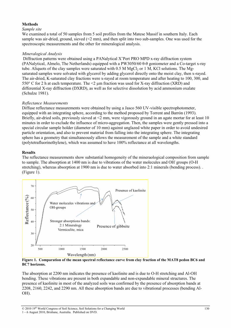
© 2010 19th World Congress of Soil Science, Soil Solutions for a Changing World
1 – 6 August 2010, Brisbane, Australia. Published on DVD. 130
Methods Sample site
We examined a total of 50 samples from 5 soil profiles from the Matese Massif in southern Italy. Each
sample was air-dried, ground, sieved (<2 mm), and then split into two sub-samples. One was used for the
spectroscopic measurements and the other for mineralogical analysis.
Mineralogical Analysis
Diffraction patterns were obtained using a PANalytical X’Pert PRO MPD x-ray diffraction system
(PANalytical, Almelo, The Netherlands) equipped with a PW3050/60 θ-θ goniometer and a Co-target x-ray
tube. Aliquots of the clay samples were saturated with 0.5 M MgCl2 or 1 M, KCl solutions. The Mg-
saturated samples were solvated with glycerol by adding glycerol directly onto the moist clay, then x-rayed.
The air-dried, K-saturated clay fractions were x-rayed at room temperature and after heating to 100, 300, and
550° C for 2 h at each temperature. The <2 µm fraction was used for X-ray diffraction (XRD) and
differential X-ray diffraction (DXRD), as well as for selective dissolution by acid ammonium oxalate
(Schulze 1981).
Reflectance Measurements
Diffuse reflectance measurements were obtained by using a Jasco 560 UV-visible spectrophotometer,
equipped with an integrating sphere, according to the method proposed by Torrent and Barrón (1993).
Briefly, air-dried soils, previously sieved at <2 mm, were vigorously ground in an agate mortar for at least 10
minutes in order to exclude the influence of micro-aggregation. Then, the samples were gently pressed into a
special circular sample holder (diameter of 10 mm) against unglazed white paper in order to avoid undesired
particle orientation, and also to prevent material from falling into the integrating sphere. The integrating
sphere has a geometry that simultaneously allows the measurement of the sample and a white standard
(polytetrafluorinethylene), which was assumed to have 100% reflectance at all wavelengths.
Results The reflectance measurements show substantial homogeneity of the mineraological composition from sample
to sample. The absorption at 1400 nm is due to vibrations of the water molecules and OH- groups (O-H
stretching), whereas absorption at 1900 nm is due to water absorbed into 2:1 minerals (bending process). .
(Figure 1).
Water molecules vibrations and
OH-groups
Stronger absorptions bands:
2:1 Mineralogy
Vermiculite, micaPresence of gibbsite
Presence of kaolinite
500 1000 1500 2000 2500
20
30
40
50
60
70
Ref
lect
ance
(%)
Wavelength (nm) Figure 1. Comparation of the mean spectral reflectance curve from clay fraction of the MAT8 pedon BC6 and
BC7 horizons.
The absorption at 2200 nm indicates the presence of kaolinite and is due to O-H stretching and Al-OH
bending. These vibrations are present in both expandable and non-expandable mineral structures. The
presence of kaolinite in most of the analyzed soils was confirmed by the presence of absorption bands at
2208, 2160, 2242, and 2290 nm. All these absorption bands are due to vibrational processes (bending Al-
OH).
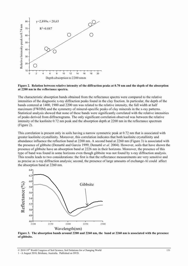
© 2010 19th World Congress of Soil Science, Soil Solutions for a Changing World
1 – 6 August 2010, Brisbane, Australia. Published on DVD. 131
y=2,899x + 20,65
R2=0.887
0 2 4 6 8 10 12 14 16 18 20
10
20
30
40
50
60
70
80R
ela
tiv
eIn
ten
sity
-pea
kto
0.7
4 n
m
Depth absorption to 2200 nmm Figure 2. Relation between relative intensity of the diffraction peaks at 0.70 nm and the depth of the absorption
at 2200 nm in the reflectance spectra.
The characteristic absorption bands obtained from the reflectance spectra were compared to the relative
intensities of the diagnostic x-ray diffraction peaks found in the clay fraction. In particular, the depth of the
bands centered at 1400, 1900 and 2200 nm was related to the relative intensity, the full width at half
maximum (FWHM) and the symmetry of mineral-specific peaks of clay minerals in the x-ray patterns.
Statistical analysis showed that none of these bands were significantly correlated with the relative intensities
of peaks derived from diffractograms. The only significant correlation observed was between the relative
intensity of the kaolinite 0.72 nm peak and the absorption depth at 2200 nm in the reflectance spectrum
(Figure 2).
This correlation is present only in soils having a narrow symmetric peak at 0.72 nm that is associated with
greater kaolinite crystallinity. Moreover, this correlation indicates that both kaolinite crystallinity and
abundance influence the reflection band at 2200 nm. A second band at 2260 nm (Figure 3) is associated with
the presence of gibbsite (Demattê and Garcia 1999; Demattê et al. 2004). However, soils that have shown the
presence of gibbsite have an absorption band at 2226 nm in their horizons. Moreover, the presence of this
type of band was found in some horizons even though gibbsite was not found by x-ray diffraction analysis.
This results leads to two considerations: the first is that the reflectance measurements are very sensitive and
as precise as x-ray diffraction analysis; second, the presence of large amounts of exchange-Al could affect
the absorption band at 2260 nm.
Gibbsite
2100 2150 2200 2250 230046
48
50
52
54
56
58
60
62
64
Ref
lect
an
ce(%
)
Wavelength(nm) Figure 3. The absorption bands around 2200 and 2260 nm, the band at 2260 nm is associated with the presence
of gibbsite.

© 2010 19th World Congress of Soil Science, Soil Solutions for a Changing World
1 – 6 August 2010, Brisbane, Australia. Published on DVD. 132
Conclusions Diffuse reflectance spectroscopy (DRS) in the VIS-NIR (400-2500 nm) region can be used as a rapid
screening method to study the clay mineralogy of volcanic soils. Diffuse reflectance of some Andisols
sampled in southern Italy is influenced by specific mineral composition. In particular, the absorption band at
2200 nm is correlated to kaolinite content, and the presence of gibbsite is correlated to an absorption band at
2260 nm. These results show that laboratory spectrometric measurements can be used to rapidly acquire
reliable information on the mineralogical properties of volcanic soils. The evaluation of diffuse soil spectra
obtained in the laboratory suggests that this approach for soil aluminum oxide estimation is comparable to
other more well known techniques such as x-ray diffraction.
References Ben-Dor E (2002) Quantitative remote sensing of soil properties. Adv. Agron. 75, 173–243.
Chang C, Laird DA, Mausbach MJ, Hurburgh Jr CR (2001) Near-infrared reflectance spectroscopy-
principal components regression analyses of soil properties. Soil Sci. Soc. Am. J. 65, 480-490.
Clark RN, King TVV, Kkejwa M, Swayze G, Vergo N (1990) High spectral resolution reflectance
spectroscopy of minerals. J. geophys. Res. 95, 12653-12680.
Demattê JA, Garcia GJ (1999) Alteration of soil properties through a weathering sequence as evaluated by
spectral reflectance. Soil Sci. Soc. Am. J. 63, 327-342.
Demattê JAM, Campos RC, Alves MC, Fiorio PR, Nanni MR (2004) Visible-NIR reflectance: a new
approach on soil evaluation. Geoderma 121, 95-112.
Farmer VC (1974) The Layer Silicates. In ‘The Infrared Spectra of Mineral’. (Ed VC Farmer) pp. 331-364.
(Mineralogical Society, London).
Schulze DG (1981) Identification of soil iron oxide minerals by differential X‑ray diffraction. Soil Sci. Soc.
Amer. J. 45, 437-440.
Sellitto VM, Fernandes RBA, Barrón V, Colombo C (2009) Comparing two different spectroscopic
techniques for the characterization of soil iron oxides: Diffuse versus bi-directional reflectance.
Geoderma 149, 2–9
Torrent J, Barrón V (1993) Laboratory Measurement of Soil Color: Theory And Practice. In ‘Soil Color’.
(Eds JM Bigham, EJCiolkosz) Soil Sci Soc Am Spec Publ 31, 21-33.
Viscarra Rossel RA, Walvoort DJJ, McBratney AB, Janik LJ, Skjemstad JO (2006) Visible, near infrared,
mid infrared or combined diffuse reflectance spectroscopy for simultaneous assessment of various soil
properties. Geoderma 13, 59–75.
Related Documents