19 Undirected graphical models (Markov random fields) 19.1 Introduction In Chapter 10, we discussed directed graphical models (DGMs), commonly known as Bayes nets. However, for some domains, being forced to choose a direction for the edges, as required by a DGM, is rather awkward. For example, consider modeling an image. We might suppose that the intensity values of neighboring pixels are correlated. We can create a DAG model with a 2d lattice topology as shown in Figure 19.1(a). This is known as a causal MRF or a Markov mesh (Abend et al. 1965). However, its conditional independence properties are rather unnatural. In particular, the Markov blanket (defined in Section 10.5) of the node X 8 in the middle is the other colored nodes (3, 4, 7, 9, 12 and 13) rather than just its 4 nearest neighbors as one might expect. An alternative is to use an undirected graphical model (UGM), also called a Markov random field (MRF) or Markov network. These do not require us to specify edge orientations, and are much more natural for some problems such as image analysis and spatial statistics. For example, an undirected 2d lattice is shown in Figure 19.1(b); now the Markov blanket of each node is just its nearest neighbors, as we show in Section 19.2. Roughly speaking, the main advantages of UGMs over DGMs are: (1) they are symmetric and therefore more “natural” for certain domains, such as spatial or relational data; and (2) discrimi- native UGMs (aka conditional random fields, or CRFs), which define conditional densities of the form p(y|x), work better than discriminative DGMs, for reasons we explain in Section 19.6.1. The main disadvantages of UGMs compared to DGMs are: (1) the parameters are less interpretable and less modular, for reasons we explain in Section 19.3; and (2) parameter estimation is com- putationally more expensive, for reasons we explain in Section 19.5. See (Domke et al. 2008) for an empirical comparison of the two approaches for an image processing task. 19.2 Conditional independence properties of UGMs 19.2.1 Key properties UGMs define CI relationships via simple graph separation as follows: for sets of nodes A, B, and C , we say x A ? G x B |x C i C separates A from B in the graph G. This means that, when we remove all the nodes in C , if there are no paths connecting any node in A to any node in B, then the CI property holds. This is called the global Markov property for UGMs. For example, in Figure 19.2(b), we have that {1, 2} ? {6, 7}|{3, 4, 5}.

Welcome message from author
This document is posted to help you gain knowledge. Please leave a comment to let me know what you think about it! Share it to your friends and learn new things together.
Transcript
19 Undirected graphical models (Markovrandom fields)
19.1 Introduction
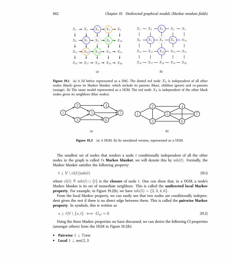
In Chapter 10, we discussed directed graphical models (DGMs), commonly known as Bayes nets.However, for some domains, being forced to choose a direction for the edges, as required bya DGM, is rather awkward. For example, consider modeling an image. We might suppose thatthe intensity values of neighboring pixels are correlated. We can create a DAG model with a 2dlattice topology as shown in Figure 19.1(a). This is known as a causal MRF or a Markov mesh(Abend et al. 1965). However, its conditional independence properties are rather unnatural. Inparticular, the Markov blanket (defined in Section 10.5) of the node X
8
in the middle is the othercolored nodes (3, 4, 7, 9, 12 and 13) rather than just its 4 nearest neighbors as one might expect.An alternative is to use an undirected graphical model (UGM), also called a Markov random
field (MRF) or Markov network. These do not require us to specify edge orientations, and aremuch more natural for some problems such as image analysis and spatial statistics. For example,an undirected 2d lattice is shown in Figure 19.1(b); now the Markov blanket of each node is justits nearest neighbors, as we show in Section 19.2.Roughly speaking, the main advantages of UGMs over DGMs are: (1) they are symmetric and
therefore more “natural” for certain domains, such as spatial or relational data; and (2) discrimi-native UGMs (aka conditional random fields, or CRFs), which define conditional densities of theform p(y|x), work better than discriminative DGMs, for reasons we explain in Section 19.6.1. Themain disadvantages of UGMs compared to DGMs are: (1) the parameters are less interpretableand less modular, for reasons we explain in Section 19.3; and (2) parameter estimation is com-putationally more expensive, for reasons we explain in Section 19.5. See (Domke et al. 2008) foran empirical comparison of the two approaches for an image processing task.
19.2 Conditional independence properties of UGMs
19.2.1 Key properties
UGMs define CI relationships via simple graph separation as follows: for sets of nodes A, B,and C , we say xA ?G xB |xC i� C separates A from B in the graph G. This means that,when we remove all the nodes in C , if there are no paths connecting any node in A to anynode in B, then the CI property holds. This is called the global Markov property for UGMs.For example, in Figure 19.2(b), we have that {1, 2} ? {6, 7}|{3, 4, 5}.
662 Chapter 19. Undirected graphical models (Markov random fields)
X1 X2 X3 X4 X5
X6 X7 X8 X9 X10
X11 X12 X13 X14 X15
X16 X17 X18 X19 X20
(a)
X1 X2 X3 X4 X5
X6 X7 X8 X9 X10
X11 X12 X13 X14 X15
X16 X17 X18 X19 X20
(b)
Figure 19.1 (a) A 2d lattice represented as a DAG. The dotted red node X8
is independent of all othernodes (black) given its Markov blanket, which include its parents (blue), children (green) and co-parents(orange). (b) The same model represented as a UGM. The red node X
8
is independent of the other blacknodes given its neighbors (blue nodes).
1
2
3
5
4
6
7
(a)
1
2
3
5
4
6
7
(b)
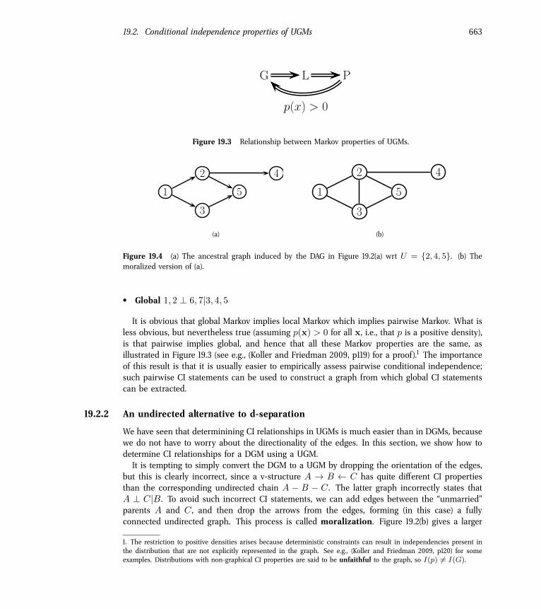
Figure 19.2 (a) A DGM. (b) Its moralized version, represented as a UGM.
The smallest set of nodes that renders a node t conditionally independent of all the othernodes in the graph is called t’s Markov blanket; we will denote this by mb(t). Formally, theMarkov blanket satisfies the following property:
t ? V \ cl(t)|mb(t) (19.1)
where cl(t) , mb(t) [ {t} is the closure of node t. One can show that, in a UGM, a node’sMarkov blanket is its set of immediate neighbors. This is called the undirected local Markovproperty. For example, in Figure 19.2(b), we have mb(5) = {2, 3, 4, 6}.From the local Markov property, we can easily see that two nodes are conditionally indepen-
dent given the rest if there is no direct edge between them. This is called the pairwise Markovproperty. In symbols, this is written as
s ? t|V \ {s, t} () Gst = 0 (19.2)
Using the three Markov properties we have discussed, we can derive the following CI properties(amongst others) from the UGM in Figure 19.2(b):
• Pairwise 1 ? 7|rest• Local 1 ? rest|2, 3
19.2. Conditional independence properties of UGMs 663
G L P
p(x) > 0
Figure 19.3 Relationship between Markov properties of UGMs.
1
2
3
5
4
(a)
1
2
3
5
4
(b)
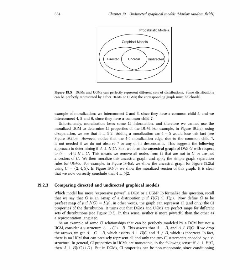
Figure 19.4 (a) The ancestral graph induced by the DAG in Figure 19.2(a) wrt U = {2, 4, 5}. (b) Themoralized version of (a).
• Global 1, 2 ? 6, 7|3, 4, 5
It is obvious that global Markov implies local Markov which implies pairwise Markov. What isless obvious, but nevertheless true (assuming p(x) > 0 for all x, i.e., that p is a positive density),is that pairwise implies global, and hence that all these Markov properties are the same, asillustrated in Figure 19.3 (see e.g., (Koller and Friedman 2009, p119) for a proof).1 The importanceof this result is that it is usually easier to empirically assess pairwise conditional independence;such pairwise CI statements can be used to construct a graph from which global CI statementscan be extracted.
19.2.2 An undirected alternative to d-separation
We have seen that determinining CI relationships in UGMs is much easier than in DGMs, becausewe do not have to worry about the directionality of the edges. In this section, we show how todetermine CI relationships for a DGM using a UGM.It is tempting to simply convert the DGM to a UGM by dropping the orientation of the edges,
but this is clearly incorrect, since a v-structure A ! B C has quite di�erent CI propertiesthan the corresponding undirected chain A � B � C . The latter graph incorrectly states thatA ? C|B. To avoid such incorrect CI statements, we can add edges between the “unmarried”parents A and C , and then drop the arrows from the edges, forming (in this case) a fullyconnected undirected graph. This process is called moralization. Figure 19.2(b) gives a larger
1. The restriction to positive densities arises because deterministic constraints can result in independencies present inthe distribution that are not explicitly represented in the graph. See e.g., (Koller and Friedman 2009, p120) for someexamples. Distributions with non-graphical CI properties are said to be unfaithful to the graph, so I(p) 6= I(G).
664 Chapter 19. Undirected graphical models (Markov random fields)
3UREDELOLVWLF�0RGHOV
*UDSKLFDO�0RGHOV
'LUHFWHG 8QGLUHFWHG&KRUGDO
Figure 19.5 DGMs and UGMs can perfectly represent di�erent sets of distributions. Some distributionscan be perfectly represented by either DGMs or UGMs; the corresponding graph must be chordal.
example of moralization: we interconnect 2 and 3, since they have a common child 5, and weinterconnect 4, 5 and 6, since they have a common child 7.Unfortunately, moralization loses some CI information, and therefore we cannot use the
moralized UGM to determine CI properties of the DGM. For example, in Figure 19.2(a), usingd-separation, we see that 4 ? 5|2. Adding a moralization arc 4 � 5 would lose this fact (seeFigure 19.2(b)). However, notice that the 4-5 moralization edge, due to the common child 7,is not needed if we do not observe 7 or any of its descendants. This suggests the followingapproach to determining if A ? B|C . First we form the ancestral graph of DAG G with respectto U = A [ B [ C . This means we remove all nodes from G that are not in U or are notancestors of U . We then moralize this ancestral graph, and apply the simple graph separationrules for UGMs. For example, in Figure 19.4(a), we show the ancestral graph for Figure 19.2(a)using U = {2, 4, 5}. In Figure 19.4(b), we show the moralized version of this graph. It is clearthat we now correctly conclude that 4 ? 5|2.
19.2.3 Comparing directed and undirected graphical models
Which model has more “expressive power”, a DGM or a UGM? To formalize this question, recallthat we say that G is an I-map of a distribution p if I(G) ✓ I(p). Now define G to beperfect map of p if I(G) = I(p), in other words, the graph can represent all (and only) the CIproperties of the distribution. It turns out that DGMs and UGMs are perfect maps for di�erentsets of distributions (see Figure 19.5). In this sense, neither is more powerful than the other asa representation language.As an example of some CI relationships that can be perfectly modeled by a DGM but not a
UGM, consider a v-structure A! C B. This asserts that A ? B, and A 6? B|C . If we dropthe arrows, we get A�C �B, which asserts A ? B|C and A 6? B, which is incorrect. In fact,there is no UGM that can precisely represent all and only the two CI statements encoded by a v-structure. In general, CI properties in UGMs are monotonic, in the following sense: if A ? B|C ,then A ? B|(C [ D). But in DGMs, CI properties can be non-monotonic, since conditioning
19.3. Parameterization of MRFs 665
C
(a) (b) (c)
A
D BBD
A
C
BD
A
C
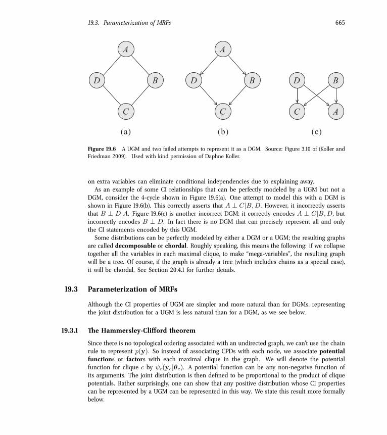
Figure 19.6 A UGM and two failed attempts to represent it as a DGM. Source: Figure 3.10 of (Koller andFriedman 2009). Used with kind permission of Daphne Koller.
on extra variables can eliminate conditional independencies due to explaining away.As an example of some CI relationships that can be perfectly modeled by a UGM but not a
DGM, consider the 4-cycle shown in Figure 19.6(a). One attempt to model this with a DGM isshown in Figure 19.6(b). This correctly asserts that A ? C|B, D. However, it incorrectly assertsthat B ? D|A. Figure 19.6(c) is another incorrect DGM: it correctly encodes A ? C|B, D, butincorrectly encodes B ? D. In fact there is no DGM that can precisely represent all and onlythe CI statements encoded by this UGM.Some distributions can be perfectly modeled by either a DGM or a UGM; the resulting graphs
are called decomposable or chordal. Roughly speaking, this means the following: if we collapsetogether all the variables in each maximal clique, to make “mega-variables”, the resulting graphwill be a tree. Of course, if the graph is already a tree (which includes chains as a special case),it will be chordal. See Section 20.4.1 for further details.
19.3 Parameterization of MRFs
Although the CI properties of UGM are simpler and more natural than for DGMs, representingthe joint distribution for a UGM is less natural than for a DGM, as we see below.
19.3.1 The Hammersley-Cli�ord theorem
Since there is no topological ordering associated with an undirected graph, we can’t use the chainrule to represent p(y). So instead of associating CPDs with each node, we associate potentialfunctions or factors with each maximal clique in the graph. We will denote the potentialfunction for clique c by c(yc|✓c). A potential function can be any non-negative function ofits arguments. The joint distribution is then defined to be proportional to the product of cliquepotentials. Rather surprisingly, one can show that any positive distribution whose CI propertiescan be represented by a UGM can be represented in this way. We state this result more formallybelow.
666 Chapter 19. Undirected graphical models (Markov random fields)
Theorem 19.3.1 (Hammersley-Cli�ord). A positive distribution p(y) > 0 satisfies the CI prop-erties of an undirected graph G i� p can be represented as a product of factors, one per maximalclique, i.e.,
p(y|✓) =
1
Z(✓)
Y
c2C c(yc|✓c) (19.3)
where C is the set of all the (maximal) cliques of G, and Z(✓) is the partition function given by
Z(✓) ,X
x
Y
c2C c(yc|✓c) (19.4)
Note that the partition function is what ensures the overall distribution sums to 1.2
The proof was never published, but can be found in e.g., (Koller and Friedman 2009).For example, consider the MRF in Figure 10.1(b). If p satisfies the CI properties of this graph
then we can write p as follows:
p(y|✓) =
1
Z(✓)
123
(y1
, y2
, y3
) 234
(y2
, y3
, y4
) 35
(y3
, y5
) (19.5)
where
Z =
X
y
123
(y1
, y2
, y3
) 234
(y2
, y3
, y4
) 35
(y3
, y5
) (19.6)
There is a deep connection between UGMs and statistical physics. In particular, there is amodel known as the Gibbs distribution, which can be written as follows:
p(y|✓) =
1
Z(✓)exp(�
X
c
E(yc|✓c)) (19.7)
where E(yc) > 0 is the energy associated with the variables in clique c. We can convert this toa UGM by defining
c(yc|✓c) = exp(�E(yc|✓c)) (19.8)
We see that high probability states correspond to low energy configurations. Models of this formare known as energy based models, and are commonly used in physics and biochemistry, aswell as some branches of machine learning (LeCun et al. 2006).Note that we are free to restrict the parameterization to the edges of the graph, rather than
the maximal cliques. This is called a pairwise MRF. In Figure 10.1(b), we get
p(y|✓) / 12
(y1
, y2
) 13
(y1
, y3
) 23
(y2
, y3
) 24
(y2
, y4
) 34
(y3
, y4
) 35
(y3
, y5
) (19.9)
/Y
s⇠t
st(ys, yt) (19.10)
This form is widely used due to its simplicity, although it is not as general.
2. The partition function is denoted by Z because of the German word Zustandssumme, which means “sum over states”.This reflects the fact that a lot of pioneering working in statistical physics was done by German speakers.
19.3. Parameterization of MRFs 667
19.3.2 Representing potential functions
If the variables are discrete, we can represent the potential or energy functions as tables of(non-negative) numbers, just as we did with CPTs. However, the potentials are not probabilities.Rather, they represent the relative “compatibility” between the di�erent assignments to thepotential. We will see some examples of this below.A more general approach is to define the log potentials as a linear function of the parameters:
log c(yc) , �c(yc)T✓c (19.11)
where �c(xc) is a feature vector derived from the values of the variables yc. The resulting logprobability has the form
log p(y|✓) =
X
c
�c(yc)T✓c � log Z(✓) (19.12)
This is also known as a maximum entropy or a log-linear model.For example, consider a pairwise MRF, where for each edge, we associate a feature vector of
length K2 as follows:
�st(ys, yt) = [. . . , I(ys = j, yt = k), . . .] (19.13)
If we have a weight for each feature, we can convert this into a K ⇥K potential function asfollows:
st(ys = j, yt = k) = exp([✓Tst�st]jk) = exp(✓st(j, k)) (19.14)
So we see that we can easily represent tabular potentials using a log-linear form. But thelog-linear form is more general.To see why this is useful, suppose we are interested in making a probabilistic model of English
spelling. Since certain letter combinations occur together quite frequently (e.g., “ing”), we willneed higher order factors to capture this. Suppose we limit ourselves to letter trigrams. Atabular potential still has 26
3
= 17, 576 parameters in it. However, most of these triples willnever occur.An alternative approach is to define indicator functions that look for certain “special” triples,
such as “ing”, “qu-”, etc. Then we can define the potential on each trigram as follows:
(yt�1
, yt, yt+1
) = exp(
X
k
✓k�k(yt�1
, yt, yt+1
)) (19.15)
where k indexes the di�erent features, corresponding to “ing”, “qu-”, etc., and �k is the corre-sponding binary feature function. By tying the parameters across locations, we can define theprobability of a word of any length using
p(y|✓) / exp(
X
t
X
k
✓k�k(yt�1
, yt, yt+1
)) (19.16)
This raises the question of where these feature functions come from. In many applications,they are created by hand to reflect domain knowledge (we will see examples later), but it is alsopossible to learn them from data, as we discuss in Section 19.5.6.
668 Chapter 19. Undirected graphical models (Markov random fields)
19.4 Examples of MRFs
In this section, we show how several popular probability models can be conveniently expressedas UGMs.
19.4.1 Ising model
The Ising model is an example of an MRF that arose from statistical physics.3 It was originallyused for modeling the behavior of magnets. In particular, let ys 2 {�1, +1} represent the spinof an atom, which can either be spin down or up. In some magnets, called ferro-magnets,neighboring spins tend to line up in the same direction, whereas in other kinds of magnets,called anti-ferromagnets, the spins “want” to be di�erent from their neighbors.We can model this as an MRF as follows. We create a graph in the form of a 2D or 3D lattice,
and connect neighboring variables, as in Figure 19.1(b). We then define the following pairwiseclique potential:
st(ys, yt) =
✓
ewst e�w
st
e�wst ew
st
◆
(19.17)
Here wst is the coupling strength between nodes s and t. If two nodes are not connected inthe graph, we set wst = 0. We assume that the weight matrix W is symmetric, so wst = wts.Often we assume all edges have the same strength, so wst = J (assuming wst 6= 0).If all the weights are positive, J > 0, then neighboring spins are likely to be in the same
state; this can be used to model ferromagnets, and is an example of an associative Markovnetwork. If the weights are su�ciently strong, the corresponding probability distribution willhave two modes, corresponding to the all +1’s state and the all -1’s state. These are called theground states of the system.If all of the weights are negative, J < 0, then the spins want to be di�erent from their
neighbors; this can be used to model an anti-ferromagnet, and results in a frustrated system,in which not all the constraints can be satisfied at the same time. The corresponding probabilitydistribution will have multiple modes. Interestingly, computing the partition function Z(J) canbe done in polynomial time for associative Markov networks, but is NP-hard in general (Cipra2000).There is an interesting analogy between Ising models and Gaussian graphical models. First,
assuming yt 2 {�1, +1}, we can write the unnormalized log probability of an Ising model asfollows:
log p(y) = �X
s⇠t
yswstyt = �1
2
yT Wy (19.18)
(The factor of 1
2
arises because we sum each edge twice.) If wst = J > 0, we get a low energy(and hence high probability) if neighboring states agree.Sometimes there is an external field, which is an energy term which is added to each spin.
This can be modelled using a local energy term of the form �bT y, where b is sometimes called
3. Ernst Ising was a German-American physicist, 1900–1998.
19.4. Examples of MRFs 669
a bias term. The modified distribution is given by
log p(y) = �X
s⇠t
wstysyt +
X
s
bsys = �1
2
yT Wy + bT y (19.19)
where ✓ = (W,b).If we define ⌃�1
= W, µ , ⌃b, and c , 1
2
µT ⌃�1µ, we can rewrite this in a form thatlooks similar to a Gaussian:
p(y) / exp(�1
2
(y � µ)
T ⌃�1
(y � µ) + c) (19.20)
One very important di�erence is that, in the case of Gaussians, the normalization constant,Z = |2⇡⌃|, requires the computation of a matrix determinant, which can be computed inO(D3
) time, whereas in the case of the Ising model, the normalization constant requiressumming over all 2
D bit vectors; this is equivalent to computing the matrix permanent, whichis NP-hard in general (Jerrum et al. 2004).
19.4.2 Hopfield networks
A Hopfield network (Hopfield 1982) is a fully connected Ising model with a symmetric weightmatrix, W = WT . These weights, plus the bias terms b, can be learned from training datausing (approximate) maximum likelihood, as described in Section 19.5.4
The main application of Hopfield networks is as an associative memory or content ad-dressable memory. The idea is this: suppose we train on a set of fully observed bit vectors,corresponding to patterns we want to memorize. Then, at test time, we present a partial patternto the network. We would like to estimate the missing variables; this is called pattern com-pletion. See Figure 19.7 for an example. This can be thought of as retrieving an example frommemory based on a piece of the example itself, hence the term “associative memory”.Since exact inference is intractable in this model, it is standard to use a coordinate descent
algorithm known as iterative conditional modes (ICM), which just sets each node to its mostlikely (lowest energy) state, given all its neighbors. The full conditional can be shown to be
p(ys = 1|y�s,✓) = sigm(wTs,:y�s + bs) (19.21)
Picking the most probable state amounts to using the rule y⇤s = 1 if
P
t wstyt > �bs and usingy⇤
s = 0 otherwise. (Much better inference algorithms will be discussed later in this book.)Since inference is deterministic, it is also possible to interpret this model as a recurrent
neural network. (This is quite di�erent from the feedforward neural nets studied in Section 16.5;they are univariate conditional density models of the form p(y|x,✓) which can only be used forsupervised learning.) See (Hertz et al. 1991) for further details on Hopfield networks.A Boltzmann machine generalizes the Hopfield / Ising model by including some hidden
nodes, which makes the model representationally more powerful. Inference in such modelsoften uses Gibbs sampling, which is a stochastic version of ICM (see Section 24.2 for details).
4. Computing the parameter MLE works much better than the outer product rule proposed in (Hopfield 1982), becauseit not only lowers the energy of the observed patterns, but it also raises the energy of the non-observed patterns, inorder to make the distribution sum to one (Hillar et al. 2012).
670 Chapter 19. Undirected graphical models (Markov random fields)
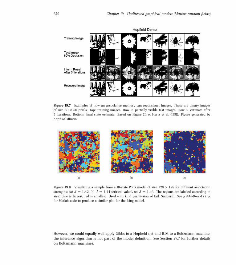
Figure 19.7 Examples of how an associative memory can reconstruct images. These are binary imagesof size 50 ⇥ 50 pixels. Top: training images. Row 2: partially visible test images. Row 3: estimate after5 iterations. Bottom: final state estimate. Based on Figure 2.1 of Hertz et al. (1991). Figure generated byhopfieldDemo.
(a) (b) (c)
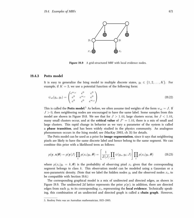
Figure 19.8 Visualizing a sample from a 10-state Potts model of size 128⇥ 128 for di�erent associationstrengths: (a) J = 1.42, (b) J = 1.44 (crirical value), (c) J = 1.46. The regions are labeled according tosize: blue is largest, red is smallest. Used with kind permission of Erik Sudderth. See gibbsDemoIsingfor Matlab code to produce a similar plot for the Ising model.
However, we could equally well apply Gibbs to a Hopfield net and ICM to a Boltzmann machine:the inference algorithm is not part of the model definition. See Section 27.7 for further detailson Boltzmann machines.
19.4. Examples of MRFs 671
xs xt
ys yt
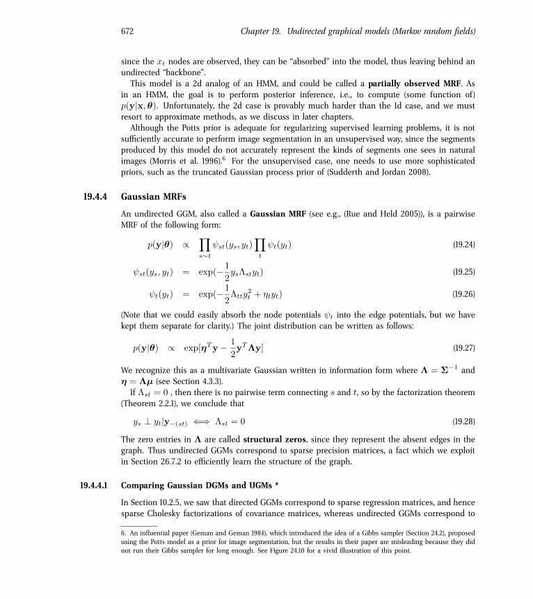
Figure 19.9 A grid-structured MRF with local evidence nodes.
19.4.3 Potts model
It is easy to generalize the Ising model to multiple discrete states, yt 2 {1, 2, . . . , K}. Forexample, if K = 3, we use a potential function of the following form:
st(ys, yt) =
0
@
ewst e0 e0
e0 ewst e0
e0 e0 ewst
1
A (19.22)
This is called the Potts model.5 As before, we often assume tied weights of the form wst = J . IfJ > 0, then neighboring nodes are encouraged to have the same label. Some samples from thismodel are shown in Figure 19.8. We see that for J > 1.44, large clusters occur, for J < 1.44,many small clusters occur, and at the critical value of J⇤
= 1.44, there is a mix of small andlarge clusters. This rapid change in behavior as we vary a parameter of the system is calleda phase transition, and has been widely studied in the physics community. An analogousphenomenon occurs in the Ising model; see (MacKay 2003, ch 31) for details.The Potts model can be used as a prior for image segmentation, since it says that neighboring
pixels are likely to have the same discrete label and hence belong to the same segment. We cancombine this prior with a likelihood term as follows:
p(y,x|✓) = p(y|J)
Y
t
p(xt|yt,✓) =
"
1
Z(J)
Y
s⇠t
(ys, yt; J)
#
Y
t
p(xt|yt,✓) (19.23)
where p(xt|yt = k,✓) is the probability of observing pixel xt given that the correspondingsegment belongs to class k. This observation model can be modeled using a Gaussian or anon-parametric density. (Note that we label the hidden nodes yt and the observed nodes xt, tobe compatible with Section 19.6.)The corresponding graphical model is a mix of undirected and directed edges, as shown in
Figure 19.9. The undirected 2d lattice represents the prior p(y); in addition, there are directededges from each yt to its corresponding xt, representing the local evidence. Technically speak-ing, this combination of an undirected and directed graph is called a chain graph. However,
5. Renfrey Potts was an Australian mathematician, 1925–2005.
672 Chapter 19. Undirected graphical models (Markov random fields)
since the xt nodes are observed, they can be “absorbed” into the model, thus leaving behind anundirected “backbone”.This model is a 2d analog of an HMM, and could be called a partially observed MRF. As
in an HMM, the goal is to perform posterior inference, i.e., to compute (some function of)p(y|x,✓). Unfortunately, the 2d case is provably much harder than the 1d case, and we mustresort to approximate methods, as we discuss in later chapters.Although the Potts prior is adequate for regularizing supervised learning problems, it is not
su�ciently accurate to perform image segmentation in an unsupervised way, since the segmentsproduced by this model do not accurately represent the kinds of segments one sees in naturalimages (Morris et al. 1996).6 For the unsupervised case, one needs to use more sophisticatedpriors, such as the truncated Gaussian process prior of (Sudderth and Jordan 2008).
19.4.4 Gaussian MRFs
An undirected GGM, also called a Gaussian MRF (see e.g., (Rue and Held 2005)), is a pairwiseMRF of the following form:
p(y|✓) /Y
s⇠t
st(ys, yt)
Y
t
t(yt) (19.24)
st(ys, yt) = exp(�1
2
ys⇤styt) (19.25)
t(yt) = exp(�1
2
⇤tty2
t + ⌘tyt) (19.26)
(Note that we could easily absorb the node potentials t into the edge potentials, but we havekept them separate for clarity.) The joint distribution can be written as follows:
p(y|✓) / exp[⌘T y � 1
2
yT ⇤y] (19.27)
We recognize this as a multivariate Gaussian written in information form where ⇤ = ⌃�1 and⌘ = ⇤µ (see Section 4.3.3).If ⇤st = 0 , then there is no pairwise term connecting s and t, so by the factorization theorem
(Theorem 2.2.1), we conclude that
ys ? yt|y�(st) () ⇤st = 0 (19.28)
The zero entries in ⇤ are called structural zeros, since they represent the absent edges in thegraph. Thus undirected GGMs correspond to sparse precision matrices, a fact which we exploitin Section 26.7.2 to e�ciently learn the structure of the graph.
19.4.4.1 Comparing Gaussian DGMs and UGMs *
In Section 10.2.5, we saw that directed GGMs correspond to sparse regression matrices, and hencesparse Cholesky factorizations of covariance matrices, whereas undirected GGMs correspond to
6. An influential paper (Geman and Geman 1984), which introduced the idea of a Gibbs sampler (Section 24.2), proposedusing the Potts model as a prior for image segmentation, but the results in their paper are misleading because they didnot run their Gibbs sampler for long enough. See Figure 24.10 for a vivid illustration of this point.
19.4. Examples of MRFs 673
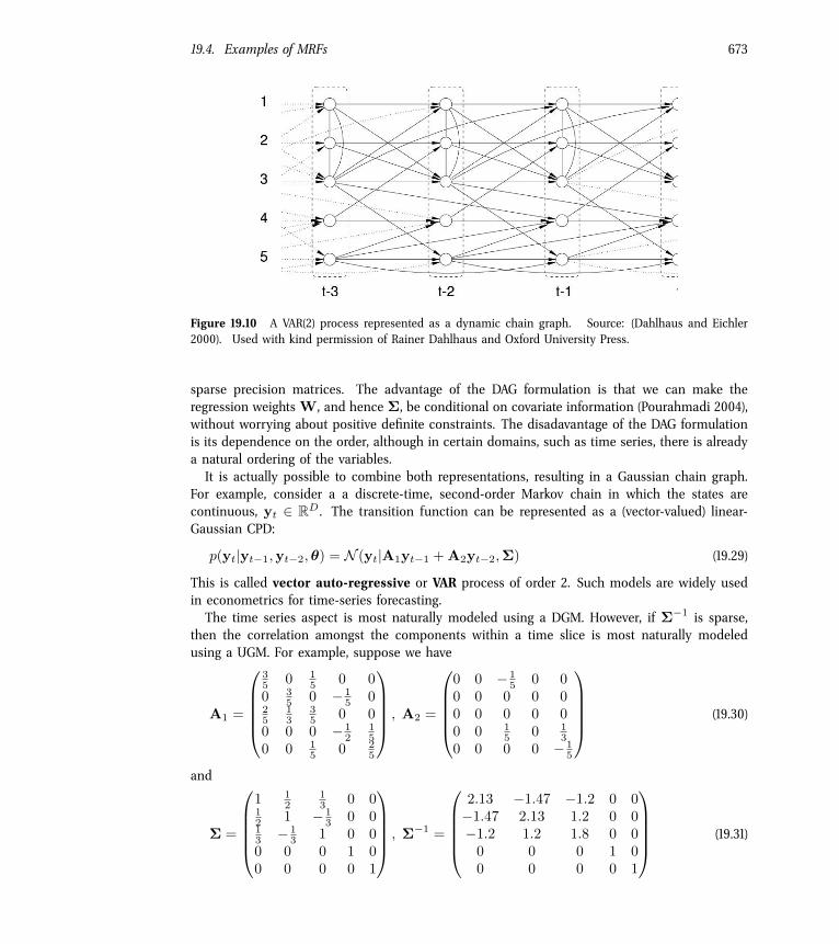
Figure 19.10 A VAR(2) process represented as a dynamic chain graph. Source: (Dahlhaus and Eichler2000). Used with kind permission of Rainer Dahlhaus and Oxford University Press.
sparse precision matrices. The advantage of the DAG formulation is that we can make theregression weights W, and hence ⌃, be conditional on covariate information (Pourahmadi 2004),without worrying about positive definite constraints. The disadavantage of the DAG formulationis its dependence on the order, although in certain domains, such as time series, there is alreadya natural ordering of the variables.It is actually possible to combine both representations, resulting in a Gaussian chain graph.
For example, consider a a discrete-time, second-order Markov chain in which the states arecontinuous, yt 2 RD . The transition function can be represented as a (vector-valued) linear-Gaussian CPD:
p(yt|yt�1
,yt�2
,✓) = N (yt|A1
yt�1
+ A2
yt�2
,⌃) (19.29)
This is called vector auto-regressive or VAR process of order 2. Such models are widely usedin econometrics for time-series forecasting.The time series aspect is most naturally modeled using a DGM. However, if ⌃�1 is sparse,
then the correlation amongst the components within a time slice is most naturally modeledusing a UGM. For example, suppose we have
A1
=
0
B
B
B
B
@
3
5
0
1
5
0 0
0
3
5
0 � 1
5
0
2
5
1
3
3
5
0 0
0 0 0 � 1
2
1
5
0 0
1
5
0
2
5
1
C
C
C
C
A
, A2
=
0
B
B
B
B
@
0 0 � 1
5
0 0
0 0 0 0 0
0 0 0 0 0
0 0
1
5
0
1
3
0 0 0 0 � 1
5
1
C
C
C
C
A
(19.30)
and
⌃ =
0
B
B
B
B
@
1
1
2
1
3
0 0
1
2
1 � 1
3
0 0
1
3
� 1
3
1 0 0
0 0 0 1 0
0 0 0 0 1
1
C
C
C
C
A
, ⌃�1
=
0
B
B
B
B
@
2.13 �1.47 �1.2 0 0
�1.47 2.13 1.2 0 0
�1.2 1.2 1.8 0 0
0 0 0 1 0
0 0 0 0 1
1
C
C
C
C
A
(19.31)
674 Chapter 19. Undirected graphical models (Markov random fields)
<� <� <�
(a)
<� <� <�
=� =�
(b)
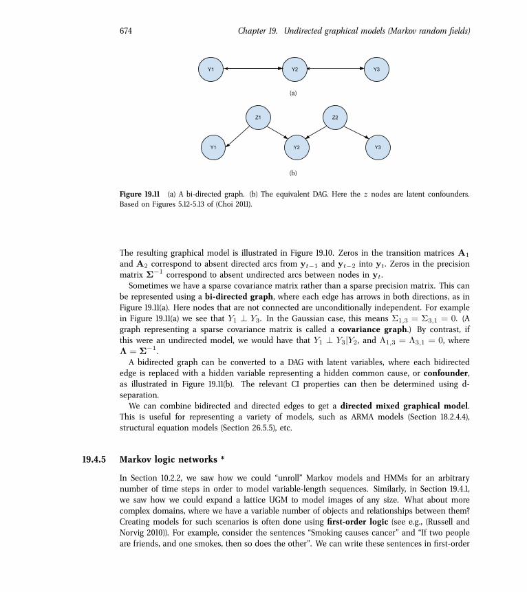
Figure 19.11 (a) A bi-directed graph. (b) The equivalent DAG. Here the z nodes are latent confounders.Based on Figures 5.12-5.13 of (Choi 2011).
The resulting graphical model is illustrated in Figure 19.10. Zeros in the transition matrices A1
and A2
correspond to absent directed arcs from yt�1
and yt�2
into yt. Zeros in the precisionmatrix ⌃�1 correspond to absent undirected arcs between nodes in yt.Sometimes we have a sparse covariance matrix rather than a sparse precision matrix. This can
be represented using a bi-directed graph, where each edge has arrows in both directions, as inFigure 19.11(a). Here nodes that are not connected are unconditionally independent. For examplein Figure 19.11(a) we see that Y
1
? Y3
. In the Gaussian case, this means ⌃
1,3 = ⌃
3,1 = 0. (Agraph representing a sparse covariance matrix is called a covariance graph.) By contrast, ifthis were an undirected model, we would have that Y
1
? Y3
|Y2
, and ⇤
1,3 = ⇤
3,1 = 0, where⇤ = ⌃�1.A bidirected graph can be converted to a DAG with latent variables, where each bidirected
edge is replaced with a hidden variable representing a hidden common cause, or confounder,as illustrated in Figure 19.11(b). The relevant CI properties can then be determined using d-separation.We can combine bidirected and directed edges to get a directed mixed graphical model.
This is useful for representing a variety of models, such as ARMA models (Section 18.2.4.4),structural equation models (Section 26.5.5), etc.
19.4.5 Markov logic networks *
In Section 10.2.2, we saw how we could “unroll” Markov models and HMMs for an arbitrarynumber of time steps in order to model variable-length sequences. Similarly, in Section 19.4.1,we saw how we could expand a lattice UGM to model images of any size. What about morecomplex domains, where we have a variable number of objects and relationships between them?Creating models for such scenarios is often done using first-order logic (see e.g., (Russell andNorvig 2010)). For example, consider the sentences “Smoking causes cancer” and “If two peopleare friends, and one smokes, then so does the other”. We can write these sentences in first-order
19.4. Examples of MRFs 675
Friends(A,A) Smokes(A) Smokes(B) Friends(B,B)
Friends(A,B)
Friends(B,A)Cancer(A) Cancer(B)
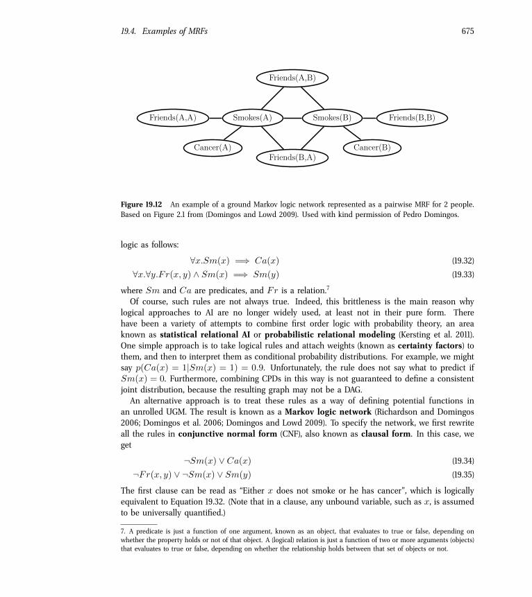
Figure 19.12 An example of a ground Markov logic network represented as a pairwise MRF for 2 people.Based on Figure 2.1 from (Domingos and Lowd 2009). Used with kind permission of Pedro Domingos.
logic as follows:
8x.Sm(x) =) Ca(x) (19.32)
8x.8y.Fr(x, y) ^ Sm(x) =) Sm(y) (19.33)
where Sm and Ca are predicates, and Fr is a relation.7
Of course, such rules are not always true. Indeed, this brittleness is the main reason whylogical approaches to AI are no longer widely used, at least not in their pure form. Therehave been a variety of attempts to combine first order logic with probability theory, an areaknown as statistical relational AI or probabilistic relational modeling (Kersting et al. 2011).One simple approach is to take logical rules and attach weights (known as certainty factors) tothem, and then to interpret them as conditional probability distributions. For example, we mightsay p(Ca(x) = 1|Sm(x) = 1) = 0.9. Unfortunately, the rule does not say what to predict ifSm(x) = 0. Furthermore, combining CPDs in this way is not guaranteed to define a consistentjoint distribution, because the resulting graph may not be a DAG.An alternative approach is to treat these rules as a way of defining potential functions in
an unrolled UGM. The result is known as a Markov logic network (Richardson and Domingos2006; Domingos et al. 2006; Domingos and Lowd 2009). To specify the network, we first rewriteall the rules in conjunctive normal form (CNF), also known as clausal form. In this case, weget
¬Sm(x) _ Ca(x) (19.34)
¬Fr(x, y) _ ¬Sm(x) _ Sm(y) (19.35)
The first clause can be read as “Either x does not smoke or he has cancer”, which is logicallyequivalent to Equation 19.32. (Note that in a clause, any unbound variable, such as x, is assumedto be universally quantified.)
7. A predicate is just a function of one argument, known as an object, that evaluates to true or false, depending onwhether the property holds or not of that object. A (logical) relation is just a function of two or more arguments (objects)that evaluates to true or false, depending on whether the relationship holds between that set of objects or not.
676 Chapter 19. Undirected graphical models (Markov random fields)
Inference in first-order logic is only semi-decidable, so it is common to use a restricted subset.A common approach (as used in Prolog) is to restrict the language to Horn clauses, which areclauses that contain at most one positive literal. Essentially this means the model is a series ofif-then rules, where the right hand side of the rules (the “then” part, or consequence) has onlya single term.Once we have encoded our knowledge base as a set of clauses, we can attach weights to
each one; these weights are the parameter of the model, and they define the clique potentialsas follows:
c(xc) = exp(wc�c(xc)) (19.36)
where �c(xc) is a logical expression which evaluates clause c applied to the variables xc, andwc is the weight we attach to this clause. Roughly speaking, the weight of a clause specifiesthe probability of a world in which this clause is satisfied relative to a world in which it is notsatisfied.Now suppose there are two objects (people) in the world, Anna and Bob, which we will denote
by constant symbols A and B. We can make a ground network from the above clauses bycreating binary random variables Sx, Cx, and Fx,y for x, y 2 {A, B}, and then “wiring theseup” according to the clauses above. The result is the UGM in Figure 19.12 with 8 binary nodes.Note that we have not encoded the fact that Fr is a symmetric relation, so Fr(A, B) andFr(B, A) might have di�erent values. Similarly, we have the “degenerate” nodes Fr(A, A) andFr(B, B), since we did not enforce x 6= y in Equation 19.33. (If we add such constraints,then the model compiler, which generates the ground network, could avoid creating redundantnodes.)In summary, we can think of MLNs as a convenient way of specifying a UGM template, that
can get unrolled to handle data of arbitrary size. There are several other ways to define relationalprobabilistic models; see e.g., (Koller and Friedman 2009; Kersting et al. 2011) for details. In somecases, there is uncertainty about the number or existence of objects or relations (the so-calledopen universe problem). Section 18.6.2 gives a concrete example in the context of multi-objecttracking. See e.g., (Russell and Norvig 2010; Kersting et al. 2011) and references therein for furtherdetails.
19.5 Learning
In this section, we discuss how to perform ML and MAP parameter estimation for MRFs. We willsee that this is quite computationally expensive. For this reason, it is rare to perform Bayesianinference for the parameters of MRFs (although see (Qi et al. 2005)).
19.5.1 Training maxent models using gradient methods
Consider an MRF in log-linear form:
p(y|✓) =
1
Z(✓)exp
X
c
✓Tc �c(y)
!
(19.37)
19.5. Learning 677
where c indexes the cliques. The scaled log-likelihood is given by
`(✓) , 1
N
X
i
log p(yi|✓) =
1
N
X
i
"
X
c
✓Tc �c(yi)� log Z(✓)
#
(19.38)
Since MRFs are in the exponential family, we know that this function is convex in ✓ (seeSection 9.2.3), so it has a unique global maximum which we can find using gradient-basedoptimizers. In particular, the derivative for the weights of a particular clique, c, is given by
@`
@✓c=
1
N
X
i
�c(yi)� @
@✓clog Z(✓)
�
(19.39)
Exercise 19.1 asks you to show that the derivative of the log partition function wrt ✓c is theexpectation of the c’th feature under the model, i.e.,
@ log Z(✓)
@✓c= E [�c(y)|✓] =
X
y
�c(y)p(y|✓) (19.40)
Hence the gradient of the log likelihood is
@`
@✓c=
"
1
N
X
i
�c(yi)
#
� E [�c(y)] (19.41)
In the first term, we fix y to its observed values; this is sometimes called the clamped term.In the second term, y is free; this is sometimes called the unclamped term or contrastiveterm. Note that computing the unclamped term requires inference in the model, and this mustbe done once per gradient step. This makes UGM training much slower than DGM training.The gradient of the log likelihood can be rewritten as the expected feature vector according
to the empirical distribution minus the model’s expectation of the feature vector:
@`
@✓c= Epemp [�c(y)]� Ep(·|✓)
[�c(y)] (19.42)
At the optimum, the gradient will be zero, so the empirical distribution of the features willmatch the model’s predictions:
Epemp [�c(y)] = Ep(·|✓)
[�c(y)] (19.43)
This is called moment matching. This observation motivates a di�erent optimization algorithmwhich we discuss in Section 19.5.7.
19.5.2 Training partially observed maxent models
Suppose we have missing data and/or hidden variables in our model. In general, we canrepresent such models as follows:
p(y,h|✓) =
1
Z(✓)exp(
X
c
✓Tc �c(h,y)) (19.44)
678 Chapter 19. Undirected graphical models (Markov random fields)
The log likelihood has the form
`(✓) =
1
N
NX
i=1
log
X
h
p(yi,h|✓)!
=
1
N
NX
i=1
log
1
Z(✓)
X
h
p(yi,h|✓)!
(19.45)
where
p(y,h|✓) , exp
X
c
✓Tc �c(h,y)
!
(19.46)
is the unnormalized distribution. The termP
h
i
p(yi,hi|✓) is the same as the partition functionfor the whole model, except that y is fixed at yi. Hence the gradient is just the expected featureswhere we clamp yi, but average over h:
@
@✓clog
X
h
p(yi,h|✓)!
= E [�c(h,yi)|✓] (19.47)
So the overall gradient is given by
@`
@✓c=
1
N
X
i
{E [�c(h,yi)|✓]� E [�c(h,y)|✓]} (19.48)
The first set of expectations are computed by “clamping” the visible nodes to their observedvalues, and the second set are computed by letting the visible nodes be free. In both cases, wemarginalize over hi.An alternative approach is to use generalized EM, where we use gradient methods in the M
step. See (Koller and Friedman 2009, p956) for details.
19.5.3 Approximate methods for computing the MLEs of MRFs
When fitting a UGM there is (in general) no closed form solution for the ML or the MAP estimateof the parameters, so we need to use gradient-based optimizers. This gradient requires inference.In models where inference is intractable, learning also becomes intractable. This has motivatedvarious computationally faster alternatives to ML/MAP estimation, which we list in Table 19.1. Wedicsuss some of these alternatives below, and defer others to later sections.
19.5.4 Pseudo likelihood
One alternative to MLE is to maximize the pseudo likelihood (Besag 1975), defined as follows:
`PL(✓) ,X
y
DX
d=1
pemp
(y) log p(yd|y�d) =
1
N
NX
i=1
DX
d=1
log p(yid|yi,�d,✓) (19.49)
That is, we optimize the product of the full conditionals, also known as the composite likeli-hood (Lindsay 1988), Compare this to the objective for maximum likelihood:
`ML(✓) =
X
y
pemp
(y) log p(y|✓) =
1
N
NX
i=1
log p(yi|✓) (19.50)
19.5. Learning 679
Method Restriction Exact MLE? SectionClosed form Only Chordal MRF Exact Section 19.5.7.4IPF Only Tabular / Gaussian MRF Exact Section 19.5.7Gradient-based optimization Low tree width Exact Section 19.5.1Max-margin training Only CRFs N/A Section 19.7Pseudo-likelihood No hidden variables Approximate Section 19.5.4Stochastic ML - Exact (up to MC error) Section 19.5.5Contrastive divergence - Approximate Section 27.7.2.4Minimum probability flow Can integrate out the hiddens Approximate Sohl-Dickstein et al. (2011)
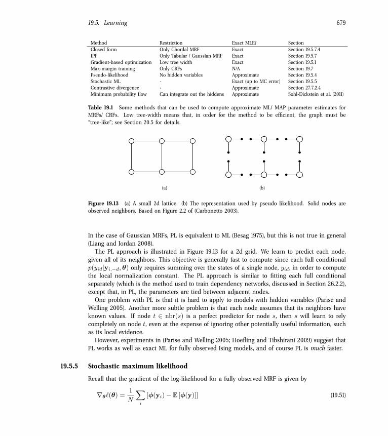
Table 19.1 Some methods that can be used to compute approximate ML/ MAP parameter estimates forMRFs/ CRFs. Low tree-width means that, in order for the method to be e�cient, the graph must be“tree-like”; see Section 20.5 for details.
(a) (b)
Figure 19.13 (a) A small 2d lattice. (b) The representation used by pseudo likelihood. Solid nodes areobserved neighbors. Based on Figure 2.2 of (Carbonetto 2003).
In the case of Gaussian MRFs, PL is equivalent to ML (Besag 1975), but this is not true in general(Liang and Jordan 2008).The PL approach is illustrated in Figure 19.13 for a 2d grid. We learn to predict each node,
given all of its neighbors. This objective is generally fast to compute since each full conditionalp(yid|yi,�d,✓) only requires summing over the states of a single node, yid, in order to computethe local normalization constant. The PL approach is similar to fitting each full conditionalseparately (which is the method used to train dependency networks, discussed in Section 26.2.2),except that, in PL, the parameters are tied between adjacent nodes.One problem with PL is that it is hard to apply to models with hidden variables (Parise and
Welling 2005). Another more subtle problem is that each node assumes that its neighbors haveknown values. If node t 2 nbr(s) is a perfect predictor for node s, then s will learn to relycompletely on node t, even at the expense of ignoring other potentially useful information, suchas its local evidence.However, experiments in (Parise and Welling 2005; Hoefling and Tibshirani 2009) suggest that
PL works as well as exact ML for fully observed Ising models, and of course PL is much faster.
19.5.5 Stochastic maximum likelihood
Recall that the gradient of the log-likelihood for a fully observed MRF is given by
r✓`(✓) =
1
N
X
i
[�(yi)� E [�(y)]] (19.51)
680 Chapter 19. Undirected graphical models (Markov random fields)
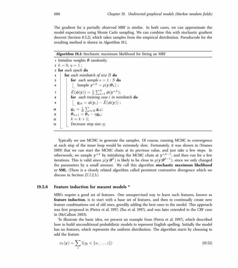
The gradient for a partially observed MRF is similar. In both cases, we can approximate themodel expectations using Monte Carlo sampling. We can combine this with stochastic gradientdescent (Section 8.5.2), which takes samples from the empirical distribution. Pseudocode for theresulting method is shown in Algorithm 19.1.
Algorithm 19.1: Stochastic maximum likelihood for fitting an MRF
1 Initialize weights ✓ randomly;2 k = 0, ⌘ = 1 ;3 for each epoch do4 for each minibatch of size B do5 for each sample s = 1 : S do6 Sample ys,k ⇠ p(y|✓k) ;
7 ˆE(�(y)) =
1
S
PSs=1
�(ys,k);
8 for each training case i in minibatch do9 gik = �(yi)� ˆE(�(y)) ;
10 gk =
1
B
P
i2B gik ;11 ✓k+1
= ✓k � ⌘gk ;12 k = k + 1;13 Decrease step size ⌘;
Typically we use MCMC to generate the samples. Of course, running MCMC to convergenceat each step of the inner loop would be extremely slow. Fortunately, it was shown in (Younes1989) that we can start the MCMC chain at its previous value, and just take a few steps. Inotherwords, we sample ys,k by initializing the MCMC chain at ys,k�1, and then run for a fewiterations. This is valid since p(y|✓k
) is likely to be close to p(y|✓k�1
), since we only changedthe parameters by a small amount. We call this algorithm stochastic maximum likelihoodor SML. (There is a closely related algorithm called persistent contrastive divergence which wediscuss in Section 27.7.2.5.)
19.5.6 Feature induction for maxent models *
MRFs require a good set of features. One unsupervised way to learn such features, known asfeature induction, is to start with a base set of features, and then to continually create newfeature combinations out of old ones, greedily adding the best ones to the model. This approachwas first proposed in (Pietra et al. 1997; Zhu et al. 1997), and was later extended to the CRF casein (McCallum 2003).To illustrate the basic idea, we present an example from (Pietra et al. 1997), which described
how to build unconditional probabilistic models to represent English spelling. Initially the modelhas no features, which represents the uniform distribution. The algorithm starts by choosing toadd the feature
�1
(y) =
X
t
I(yt 2 {a, . . . , z}) (19.52)
19.5. Learning 681
which checks if any letter is lower case or not. After the feature is added, the parameters are(re)-fit by maximum likelihood. For this feature, it turns out that ˆ✓
1
= 1.944, which means thata word with a lowercase letter in any position is about e1.944 ⇡ 7 times more likely than thesame word without a lowercase letter in that position. Some samples from this model, generatedusing (annealed) Gibbs sampling (Section 24.2), are shown below.8
m, r, xevo, ijjiir, b, to, jz, gsr, wq, vf, x, ga, msmGh, pcp, d, oziVlal,hzagh, yzop, io, advzmxnv, ijv_bolft, x, emx, kayerf, mlj, rawzyb, jp, ag,ctdnnnbg, wgdw, t, kguv, cy, spxcq, uzflbbf, dxtkkn, cxwx, jpd, ztzh, lv,zhpkvnu, l^, r, qee, nynrx, atze4n, ik, se, w, lrh, hp+, yrqyka’h, zcngotcnx,igcump, zjcjs, lqpWiqu, cefmfhc, o, lb, fdcY, tzby, yopxmvk, by, fz„ t, govyccm,ijyiduwfzo, 6xr, duh, ejv, pk, pjw, l, fl, w
The second feature added by the algorithm checks if two adjacent characters are lower case:
�2
(y) =
X
s⇠t
I(ys 2 {a, . . . , z}, yt 2 {a, . . . , z}) (19.53)
Now the model has the form
p(y) =
1
Zexp(✓
1
�1
(y) + ✓2
�2
(y)) (19.54)
Continuing in this way, the algorithm adds features for the strings s> and ing>, where >represents the end of word, and for various regular expressions such as [0-9], etc. Somesamples from the model with 1000 features, generated using (annealed) Gibbs sampling, areshown below.
was, reaser, in, there, to, will, „ was, by, homes, thing, be, reloverated,ther, which, conists, at, fores, anditing, with, Mr., proveral, the, „ ***,on’t, prolling, prothere, „ mento, at, yaou, 1, chestraing, for, have, to,intrally, of, qut, ., best, compers, ***, cluseliment, uster, of, is, deveral,this, thise, of, offect, inatever, thifer, constranded, stater, vill, in, thase,in, youse, menttering, and, ., of, in, verate, of, to
This approach of feature learning can be thought of as a form of graphical model structurelearning (Chapter 26), except it is more fine-grained: we add features that are useful, regardlessof the resulting graph structure. However, the resulting graphs can become densely connected,which makes inference (and hence parameter estimation) intractable.
19.5.7 Iterative proportional fitting (IPF) *
Consider a pairwise MRF where the potentials are represented as tables, with one parameter pervariable setting. We can represent this in log-linear form using
st(ys, yt) = exp
⇣
✓Tst[I(ys = 1, yt = 1), . . . , I(ys = K, yt = K)]
⌘
(19.55)
and similarly for t(yt). Thus the feature vectors are just indicator functions.
8. We thank John La�erty for sharing this example.
682 Chapter 19. Undirected graphical models (Markov random fields)
From Equation 19.43, we have that, at the maximum of the likelihood, the empirical expectationof the features equals the model’s expectation:
Epemp [I(ys = j, yt = k)] = Ep(·|✓)
[I(ys = j, yt = k)] (19.56)
pemp
(ys = j, yt = k) = p(ys = j, yt = k|✓) (19.57)
where pemp
is the empirical probability:
pemp
(ys = j, yt = k) =
Nst,jk
N=
PNn=1
I(yns = j, ynt = k)
N(19.58)
For a general graph, the condition that must hold at the optimum is
pemp
(yc) = p(yc|✓) (19.59)
For a special family of graphs known as decomposable graphs (defined in Section 20.4.1), onecan show that p(yc|✓) = c(yc). However, even if the graph is not decomposable, we canimagine trying to enforce this condition. This suggests an iterative coordinate ascent schemewhere at each step we compute
t+1
c (yc) = tc(yc)⇥ p
emp
(yc)
p(yc| t)
(19.60)
where the multiplication and division is elementwise. This is known as iterative proportionalfitting or IPF (Fienberg 1970; Bishop et al. 1975). See Algorithm 19.2 for the pseudocode.
Algorithm 19.2: Iterative Proportional Fitting algorithm for tabular MRFs
1 Initialize c = 1 for c = 1 : C ;2 repeat3 for c = 1 : C do4 pc = p(yc| );5 pc = p
emp
(yc);6 c = c. ⇤ p
c
pc
;
7 until converged;
19.5.7.1 Example
Let us consider a simple example from http://en.wikipedia.org/wiki/Iterative_proportional_fitting. We have two binary variables, where Y
1
indicates if the person is maleor female, and Y
2
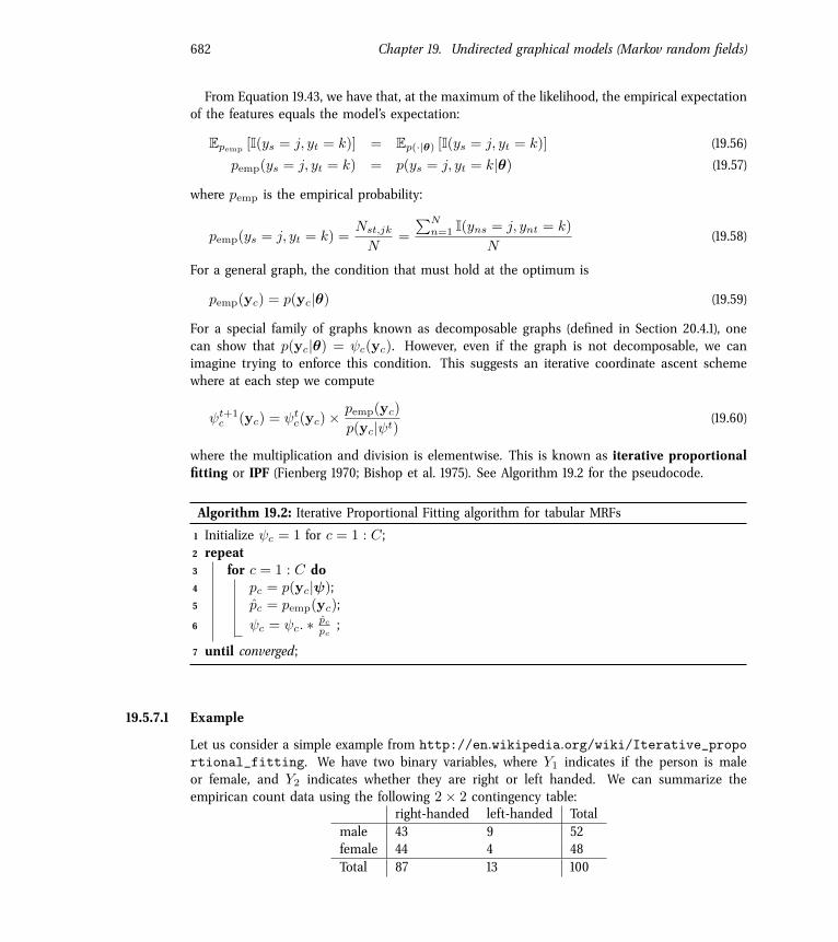
indicates whether they are right or left handed. We can summarize theempirican count data using the following 2⇥ 2 contingency table:
right-handed left-handed Totalmale 43 9 52female 44 4 48Total 87 13 100
19.5. Learning 683
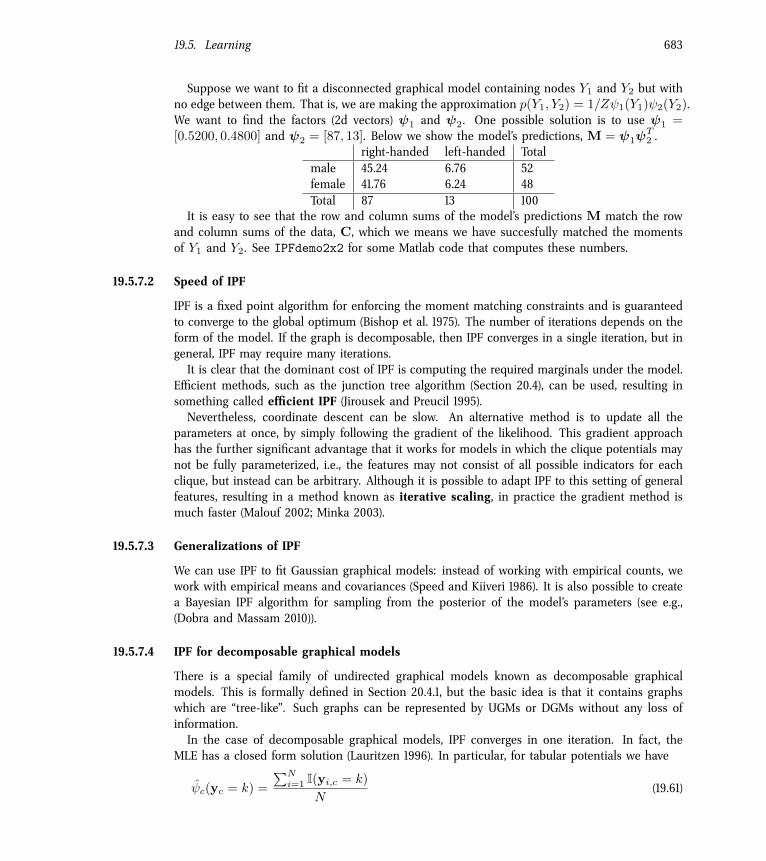
Suppose we want to fit a disconnected graphical model containing nodes Y1
and Y2
but withno edge between them. That is, we are making the approximation p(Y
1
, Y2
) = 1/Z 1
(Y1
) 2
(Y2
).We want to find the factors (2d vectors)
1
and 2
. One possible solution is to use 1
=
[0.5200, 0.4800] and 2
= [87, 13]. Below we show the model’s predictions, M = 1
T2
.right-handed left-handed Total
male 45.24 6.76 52female 41.76 6.24 48Total 87 13 100
It is easy to see that the row and column sums of the model’s predictions M match the rowand column sums of the data, C, which we means we have succesfully matched the momentsof Y
1
and Y2
. See IPFdemo2x2 for some Matlab code that computes these numbers.
19.5.7.2 Speed of IPF
IPF is a fixed point algorithm for enforcing the moment matching constraints and is guaranteedto converge to the global optimum (Bishop et al. 1975). The number of iterations depends on theform of the model. If the graph is decomposable, then IPF converges in a single iteration, but ingeneral, IPF may require many iterations.It is clear that the dominant cost of IPF is computing the required marginals under the model.
E�cient methods, such as the junction tree algorithm (Section 20.4), can be used, resulting insomething called e�cient IPF (Jirousek and Preucil 1995).Nevertheless, coordinate descent can be slow. An alternative method is to update all the
parameters at once, by simply following the gradient of the likelihood. This gradient approachhas the further significant advantage that it works for models in which the clique potentials maynot be fully parameterized, i.e., the features may not consist of all possible indicators for eachclique, but instead can be arbitrary. Although it is possible to adapt IPF to this setting of generalfeatures, resulting in a method known as iterative scaling, in practice the gradient method ismuch faster (Malouf 2002; Minka 2003).
19.5.7.3 Generalizations of IPF
We can use IPF to fit Gaussian graphical models: instead of working with empirical counts, wework with empirical means and covariances (Speed and Kiiveri 1986). It is also possible to createa Bayesian IPF algorithm for sampling from the posterior of the model’s parameters (see e.g.,(Dobra and Massam 2010)).
19.5.7.4 IPF for decomposable graphical models
There is a special family of undirected graphical models known as decomposable graphicalmodels. This is formally defined in Section 20.4.1, but the basic idea is that it contains graphswhich are “tree-like”. Such graphs can be represented by UGMs or DGMs without any loss ofinformation.In the case of decomposable graphical models, IPF converges in one iteration. In fact, the
MLE has a closed form solution (Lauritzen 1996). In particular, for tabular potentials we have
ˆ c(yc = k) =
PNi=1
I(yi,c = k)
N(19.61)
684 Chapter 19. Undirected graphical models (Markov random fields)
and for Gaussian potentials, we have
ˆµc =
PNi=1
yic
N, ˆ⌃c =
P
i(yic � ˆµc)(xic � ˆµc)T
N(19.62)
By using conjugate priors, we can also easily compute the full posterior over the model pa-rameters in the decomposable case, just as we did in the DGM case. See (Lauritzen 1996) fordetails.
19.6 Conditional random fields (CRFs)
A conditional random field or CRF (La�erty et al. 2001), sometimes a discriminative randomfield (Kumar and Hebert 2003), is just a version of an MRF where all the clique potentials areconditioned on input features:
p(y|x,w) =
1
Z(x,w)
Y
c
c(yc|x,w) (19.63)
A CRF can be thought of as a structured output extension of logistic regression, where wemodel the correlation amongst the output labels conditioned on the input features.9 We willusually assume a log-linear representation of the potentials:
c(yc|x,w) = exp(wTc �(x,yc)) (19.64)
where �(x,yc) is a feature vector derived from the global inputs x and the local set of labelsyc. We will give some examples below which will make this notation clearer.The advantage of a CRF over an MRF is analogous to the advantage of a discriminative
classifier over a generative classifier (see Section 8.6), namely, we don’t need to “waste resources”modeling things that we always observe. Instead we can focus our attention on modeling whatwe care about, namely the distribution of labels given the data.Another important advantage of CRFs is that we can make the potentials (or factors) of the
model be data-dependent. For example, in image processing applications, we may “turn o�” thelabel smoothing between two neighboring nodes s and t if there is an observed discontinuity inthe image intensity between pixels s and t. Similarly, in natural language processing problems,we can make the latent labels depend on global properties of the sentence, such as whichlanguage it is written in. It is hard to incorporate global features into generative models.The disadvantage of CRFs over MRFs is that they require labeled training data, and they
are slower to train, as we explain in Section 19.6.3. This is analogous to the strengths andweaknesses of logistic regression vs naive Bayes, discussed in Section 8.6.
19.6.1 Chain-structured CRFs, MEMMs and the label-bias problem
The most widely used kind of CRF uses a chain-structured graph to model correlation amongstneighboring labels. Such models are useful for a variety of sequence labeling tasks (see Sec-tion 19.6.2).
9. An alternative approach is to predict the label for a node i given i’s features and given the features of i’s neighbors,as opposed to conditioning on the hidden label of i’s neighbors. In general, however, this aproach needs much moredata to work well (Jensen et al. 2004).
19.6. Conditional random fields (CRFs) 685
xt!1 xt xt+1
yt!1 yt yt+1
(a)
xt!1 xt xt+1
yt!1
yt
yt+1
xg
(b)
xt!1 xt xt+1
yt!1
yt
yt+1
xg
(c)
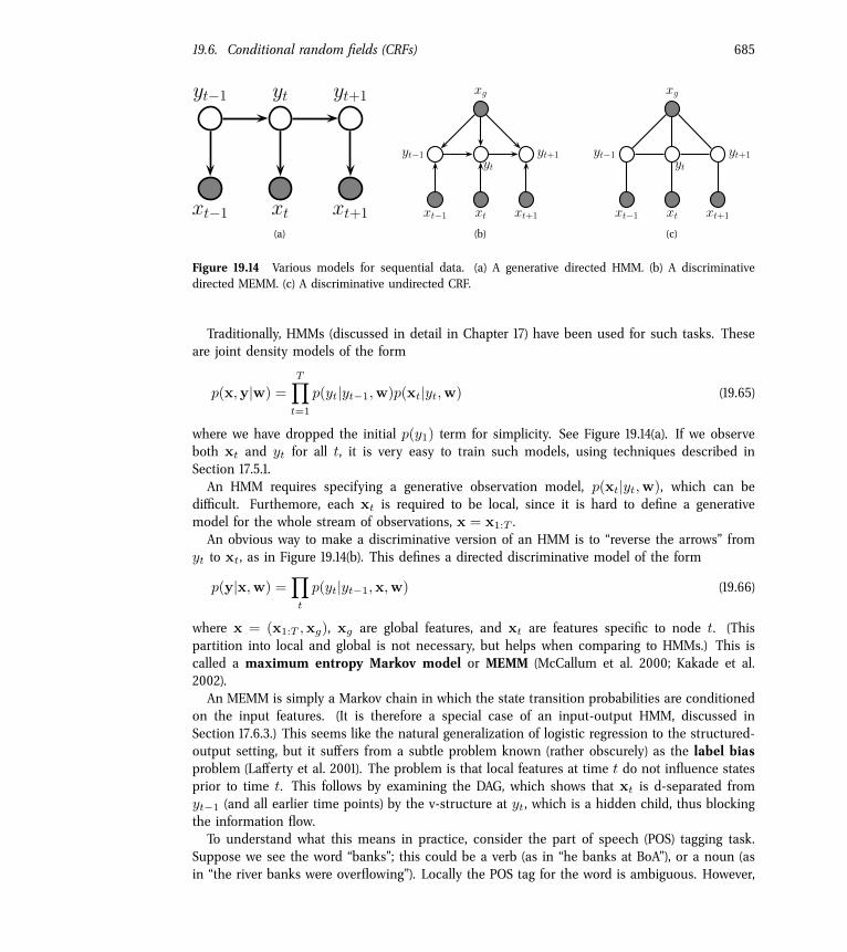
Figure 19.14 Various models for sequential data. (a) A generative directed HMM. (b) A discriminativedirected MEMM. (c) A discriminative undirected CRF.
Traditionally, HMMs (discussed in detail in Chapter 17) have been used for such tasks. Theseare joint density models of the form
p(x,y|w) =
TY
t=1
p(yt|yt�1
,w)p(xt|yt,w) (19.65)
where we have dropped the initial p(y1
) term for simplicity. See Figure 19.14(a). If we observeboth xt and yt for all t, it is very easy to train such models, using techniques described inSection 17.5.1.An HMM requires specifying a generative observation model, p(xt|yt,w), which can be
di�cult. Furthemore, each xt is required to be local, since it is hard to define a generativemodel for the whole stream of observations, x = x
1:T .An obvious way to make a discriminative version of an HMM is to “reverse the arrows” from
yt to xt, as in Figure 19.14(b). This defines a directed discriminative model of the form
p(y|x,w) =
Y
t
p(yt|yt�1
,x,w) (19.66)
where x = (x1:T ,xg), xg are global features, and xt are features specific to node t. (This
partition into local and global is not necessary, but helps when comparing to HMMs.) This iscalled a maximum entropy Markov model or MEMM (McCallum et al. 2000; Kakade et al.2002).An MEMM is simply a Markov chain in which the state transition probabilities are conditioned
on the input features. (It is therefore a special case of an input-output HMM, discussed inSection 17.6.3.) This seems like the natural generalization of logistic regression to the structured-output setting, but it su�ers from a subtle problem known (rather obscurely) as the label biasproblem (La�erty et al. 2001). The problem is that local features at time t do not influence statesprior to time t. This follows by examining the DAG, which shows that xt is d-separated fromyt�1
(and all earlier time points) by the v-structure at yt, which is a hidden child, thus blockingthe information flow.To understand what this means in practice, consider the part of speech (POS) tagging task.
Suppose we see the word “banks”; this could be a verb (as in “he banks at BoA”), or a noun (asin “the river banks were overflowing”). Locally the POS tag for the word is ambiguous. However,
686 Chapter 19. Undirected graphical models (Markov random fields)
(a) (b) (c) (d) (e)
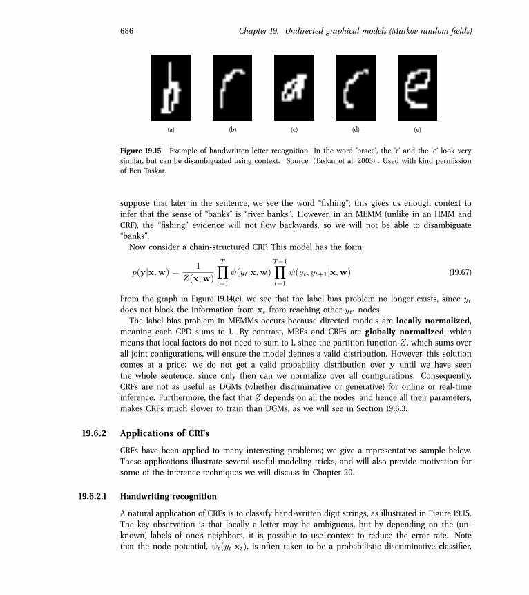
Figure 19.15 Example of handwritten letter recognition. In the word ’brace’, the ’r’ and the ’c’ look verysimilar, but can be disambiguated using context. Source: (Taskar et al. 2003) . Used with kind permissionof Ben Taskar.
suppose that later in the sentence, we see the word “fishing”; this gives us enough context toinfer that the sense of “banks” is “river banks”. However, in an MEMM (unlike in an HMM andCRF), the “fishing” evidence will not flow backwards, so we will not be able to disambiguate“banks”.Now consider a chain-structured CRF. This model has the form
p(y|x,w) =
1
Z(x,w)
TY
t=1
(yt|x,w)
T�1
Y
t=1
(yt, yt+1
|x,w) (19.67)
From the graph in Figure 19.14(c), we see that the label bias problem no longer exists, since yt
does not block the information from xt from reaching other yt0 nodes.The label bias problem in MEMMs occurs because directed models are locally normalized,
meaning each CPD sums to 1. By contrast, MRFs and CRFs are globally normalized, whichmeans that local factors do not need to sum to 1, since the partition function Z , which sums overall joint configurations, will ensure the model defines a valid distribution. However, this solutioncomes at a price: we do not get a valid probability distribution over y until we have seenthe whole sentence, since only then can we normalize over all configurations. Consequently,CRFs are not as useful as DGMs (whether discriminative or generative) for online or real-timeinference. Furthermore, the fact that Z depends on all the nodes, and hence all their parameters,makes CRFs much slower to train than DGMs, as we will see in Section 19.6.3.
19.6.2 Applications of CRFs
CRFs have been applied to many interesting problems; we give a representative sample below.These applications illustrate several useful modeling tricks, and will also provide motivation forsome of the inference techniques we will discuss in Chapter 20.
19.6.2.1 Handwriting recognition
A natural application of CRFs is to classify hand-written digit strings, as illustrated in Figure 19.15.The key observation is that locally a letter may be ambiguous, but by depending on the (un-known) labels of one’s neighbors, it is possible to use context to reduce the error rate. Notethat the node potential, t(yt|xt), is often taken to be a probabilistic discriminative classifier,
19.6. Conditional random fields (CRFs) 687
Mrs. Green spoke today in New York
(a)
(b)
Green chairs the finance committee
B-PER I-PER OTH OTH OTH B-LOC I-LOC B-PER OTHOTHOTHOTH
its withdrawal from the UALAirways rose after announcing
KEY
Begin person nameWithin person nameBegin location name
B-PERI-PERB-LOC
Within location nameNot an entitiy
I-LOCOTH
British deal
ADJ N V IN V PRP N IN NNDT
B I O O O B I O I
POS
NPIB
Begin noun phraseWithin noun phraseNot a noun phraseNounAdjective
BIONADJ
VerbPrepositionPossesive pronounDeterminer (e.g., a, an, the)
VINPRPDT
KEY
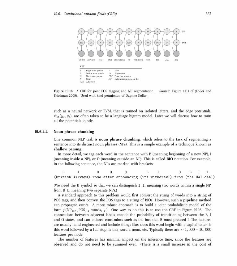
Figure 19.16 A CRF for joint POS tagging and NP segmentation. Source: Figure 4.E.1 of (Koller andFriedman 2009). Used with kind permission of Daphne Koller.
such as a neural network or RVM, that is trained on isolated letters, and the edge potentials, st(ys, yt), are often taken to be a language bigram model. Later we will discuss how to trainall the potentials jointly.
19.6.2.2 Noun phrase chunking
One common NLP task is noun phrase chunking, which refers to the task of segmenting asentence into its distinct noun phrases (NPs). This is a simple example of a technique known asshallow parsing.In more detail, we tag each word in the sentence with B (meaning beginning of a new NP), I
(meaning inside a NP), or O (meaning outside an NP). This is called BIO notation. For example,in the following sentence, the NPs are marked with brackets:
B I O O O B I O B I I(British Airways) rose after announcing (its withdrawl) from (the UAI deal)
(We need the B symbol so that we can distinguish I I, meaning two words within a single NP,from B B, meaning two separate NPs.)A standard approach to this problem would first convert the string of words into a string of
POS tags, and then convert the POS tags to a string of BIOs. However, such a pipeline methodcan propagate errors. A more robust approach is to build a joint probabilistic model of theform p(NP
1:T , POS1:T |words
1:T ). One way to do this is to use the CRF in Figure 19.16. Theconnections between adjacent labels encode the probability of transitioning between the B, Iand O states, and can enforce constraints such as the fact that B must preceed I. The featuresare usually hand engineered and include things like: does this word begin with a capital letter, isthis word followed by a full stop, is this word a noun, etc. Typically there are ⇠ 1, 000�10, 000
features per node.The number of features has minimal impact on the inference time, since the features are
observed and do not need to be summed over. (There is a small increase in the cost of
688 Chapter 19. Undirected graphical models (Markov random fields)
Mrs. Green spoke today in New York
(a)
(b)
Green chairs the finance committee
B-PER I-PER OTH OTH OTH B-LOC I-LOC B-PER OTHOTHOTHOTH
its withdrawal from the UALAirways rose after announcing
KEY
Begin person nameWithin person nameBegin location name
B-PERI-PERB-LOC
Within location nameNot an entitiy
I-LOCOTH
British deal
ADJ N V IN V PRP N IN NNDT
B I O O O B I O I
POS
NPIB
Begin noun phraseWithin noun phraseNot a noun phraseNounAdjective
BIONADJ
VerbPrepositionPossesive pronounDeterminer (e.g., a, an, the)
VINPRPDT
KEY
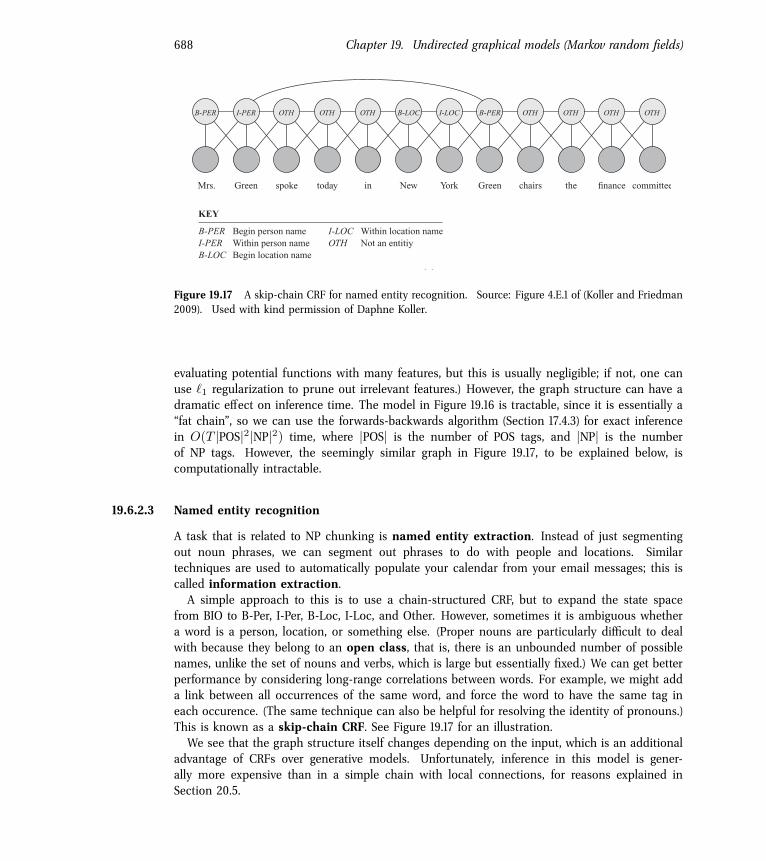
Figure 19.17 A skip-chain CRF for named entity recognition. Source: Figure 4.E.1 of (Koller and Friedman2009). Used with kind permission of Daphne Koller.
evaluating potential functions with many features, but this is usually negligible; if not, one canuse `
1
regularization to prune out irrelevant features.) However, the graph structure can have adramatic e�ect on inference time. The model in Figure 19.16 is tractable, since it is essentially a“fat chain”, so we can use the forwards-backwards algorithm (Section 17.4.3) for exact inferencein O(T |POS|2|NP|2) time, where |POS| is the number of POS tags, and |NP| is the numberof NP tags. However, the seemingly similar graph in Figure 19.17, to be explained below, iscomputationally intractable.
19.6.2.3 Named entity recognition
A task that is related to NP chunking is named entity extraction. Instead of just segmentingout noun phrases, we can segment out phrases to do with people and locations. Similartechniques are used to automatically populate your calendar from your email messages; this iscalled information extraction.A simple approach to this is to use a chain-structured CRF, but to expand the state space
from BIO to B-Per, I-Per, B-Loc, I-Loc, and Other. However, sometimes it is ambiguous whethera word is a person, location, or something else. (Proper nouns are particularly di�cult to dealwith because they belong to an open class, that is, there is an unbounded number of possiblenames, unlike the set of nouns and verbs, which is large but essentially fixed.) We can get betterperformance by considering long-range correlations between words. For example, we might adda link between all occurrences of the same word, and force the word to have the same tag ineach occurence. (The same technique can also be helpful for resolving the identity of pronouns.)This is known as a skip-chain CRF. See Figure 19.17 for an illustration.We see that the graph structure itself changes depending on the input, which is an additional
advantage of CRFs over generative models. Unfortunately, inference in this model is gener-ally more expensive than in a simple chain with local connections, for reasons explained inSection 20.5.
19.6. Conditional random fields (CRFs) 689
2006/08/03 14:15
6 SVM Learning for Interdependent and Structured Output Spaces
Figure 1.2 Natural language parsing.
e�cient computation of the discriminant function, which in the case of (1.5) is given
by
F (x,y;w) =
�
wol,lx
X
t=1
�(xt) ⌦ ⇤c
(yt)
�
+ ⌘
�
wll,lx�1
X
t=1
⇤
c(yt
) ⌦ ⇤c(yt+1
)
�
,
(1.6)
where w = wol � wll is the concatenation of weights of the two dependency types.
As indicated in Proposition 1, the inner product of the joint feature map decom-
poses into kernels over input and output spaces
h (x,y), (x0,y0)i =
lxX
t=1
lx0X
s=1
�(yt, ys)k(xt, ¯xs
) + ⌘2
lx�1
X
t=1
lx0 �1
X
s=1
�(yt, ys)�(yt+1, ys+1
).
(1.7)
where we used the equality h⇤c(�),⇤c
(�)i = �(�, �).
1.2.3 Weighted Context-Free Grammars
Parsing is the task of predicting a labeled tree y that is a particular configuration
of grammar rules generating a given sequence x = (x1, ..., xl). Let us consider a
context-free grammar in Chomsky Normal Form. The rules of this grammar are of
the form � ! �0�00, or � ! x, where �,�0,�00 2 ⌃ are non-terminals, and x 2 T are
terminals. Similar to the sequence case, we define the joint feature map (x, y) to
contain features representing inter-dependencies between labels of the nodes of the
tree (e.g. �!�0�00via ⇤
c(yrs
) ⌦ ⇤
c(yrt
) ⌦ ⇤c(y(t+1)s
)) and features representing
the dependence of labels to observations (e.g. �!⌧ via �
c(xt
) ⌦ ⇤c(yt
)). Here yrs
denotes the label of the root of a subtree spanning from xrto xs
. This definition
leads to equations similar to (1.5), (1.6) and (1.7). Extensions to this representation
is possible, for example by defining higher order features that can be induced using
kernel functions over sub-trees (Collins and Du�y, 2002).
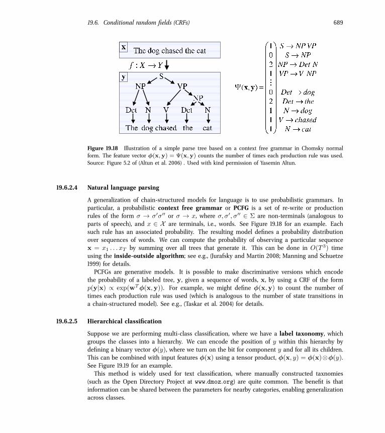
Figure 19.18 Illustration of a simple parse tree based on a context free grammar in Chomsky normalform. The feature vector �(x,y) = (x,y) counts the number of times each production rule was used.Source: Figure 5.2 of (Altun et al. 2006) . Used with kind permission of Yasemin Altun.
19.6.2.4 Natural language parsing
A generalization of chain-structured models for language is to use probabilistic grammars. Inparticular, a probabilistic context free grammar or PCFG is a set of re-write or productionrules of the form � ! �0�00 or � ! x, where �,�0,�00 2 ⌃ are non-terminals (analogous toparts of speech), and x 2 X are terminals, i.e., words. See Figure 19.18 for an example. Eachsuch rule has an associated probability. The resulting model defines a probability distributionover sequences of words. We can compute the probability of observing a particular sequencex = x
1
. . . xT by summing over all trees that generate it. This can be done in O(T 3
) timeusing the inside-outside algorithm; see e.g., (Jurafsky and Martin 2008; Manning and Schuetze1999) for details.PCFGs are generative models. It is possible to make discriminative versions which encode
the probability of a labeled tree, y, given a sequence of words, x, by using a CRF of the formp(y|x) / exp(wT�(x,y)). For example, we might define �(x,y) to count the number oftimes each production rule was used (which is analogous to the number of state transitions ina chain-structured model). See e.g., (Taskar et al. 2004) for details.
19.6.2.5 Hierarchical classification
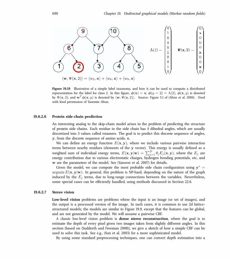
Suppose we are performing multi-class classification, where we have a label taxonomy, whichgroups the classes into a hierarchy. We can encode the position of y within this hierarchy bydefining a binary vector �(y), where we turn on the bit for component y and for all its children.This can be combined with input features �(x) using a tensor product, �(x, y) = �(x)⌦�(y).See Figure 19.19 for an example.This method is widely used for text classification, where manually constructed taxnomies
(such as the Open Directory Project at www.dmoz.org) are quite common. The benefit is thatinformation can be shared between the parameters for nearby categories, enabling generalizationacross classes.
690 Chapter 19. Undirected graphical models (Markov random fields)
2006/08/03 14:15
1.2 A Framework for Structured/Interdependent Output Learning 5
hw, (x, 2)i = hw2
,xi + hw6
,xi + hw9
,xiFigure 1.1 Classification with taxonomies.
Thus, the features �z are shared by all successor classes of z and the joint feature
representation enables generalization across classes. Figure 1.1 shows an example
of the joint feature map of the second class for a given hierarchy.
It follows immediately from (1.3) of Proposition 1 that the inner product of the
joint feature map decomposes into kernels over input and output spaces
h (x, y), (x0, y0)i = h⇤(y),⇤(y0
)i k(x,x0).
1.2.2 Label Sequence Learning
Label sequence learning is the task of predicting a sequence of labels y = (y1, . . . , yl)
for a given observation sequence x = (x1, . . . ,xl). Applications of this problem are
ubiquitous in many domains such as computational biology, information retrieval,
natural language processing and speech recognition. We denote by lx
the length of
an observation sequence, by ⌃ the set of possible labels for each individual variable
yt, and by Y(x) the set of label sequences for x. Then, Y(x) = ⌃
lx.
In order to encode the dependencies of the observation-label sequences which
are commonly realized as a Markov chain, we define to include interactions
between input features and labels (�(xt) ⌦⇤c
(yt)), as well as interactions between
neighboring label variables (⇤
c(yt
)⌦⇤c(yt+1
)) for every position t. Then, using the
stationary property, our joint feature map is a sum over all positions
(x,y) =
"
lxX
t=1
�(xt) ⌦ ⇤c
(yt)
#
�"
⌘lx�1
X
t=1
⇤
c(yt
) ⌦ ⇤c(yt+1
)
#
, (1.5)
where ⌘ � 0 is a scalar balancing the two types of contributions. Clearly, this repre-
sentation can be generalized by including higher order inter-dependencies of labels
(e. g. ⇤
c(yt
)⌦⇤c(yt+1
)⌦⇤c(yt+2
)), by including input features from a window cen-
tered at the current position (e. g. replacing �(xt) with �(xt�r, . . . ,xt, . . . ,xt+r
))
or by combining higher order output features with input features (e. g.
P
t�(xt)⌦
⇤
c(yt
) ⌦ ⇤c(yt+1
)). The important constraint on designing the feature map is the
Figure 19.19 Illustration of a simple label taxonomy, and how it can be used to compute a distributedrepresentation for the label for class 2. In this figure, �(x) = x, �(y = 2) = ⇤(2), �(x, y) is denotedby (x, 2), and wT �(x, y) is denoted by hw, (x, 2)i. Source: Figure 5.1 of (Altun et al. 2006) . Usedwith kind permission of Yasemin Altun.
19.6.2.6 Protein side-chain prediction
An interesting analog to the skip-chain model arises in the problem of predicting the structureof protein side chains. Each residue in the side chain has 4 dihedral angles, which are usuallydiscretized into 3 values called rotamers. The goal is to predict this discrete sequence of angles,y, from the discrete sequence of amino acids, x.We can define an energy function E(x,y), where we include various pairwise interaction
terms between nearby residues (elements of the y vector). This energy is usually defined as aweighted sum of individual energy terms, E(x,y|w) =
PDj=1
✓jEj(x,y), where the Ej areenergy contribution due to various electrostatic charges, hydrogen bonding potentials, etc, andw are the parameters of the model. See (Yanover et al. 2007) for details.Given the model, we can compute the most probable side chain configuration using y⇤
=
argmin E(x,y|w). In general, this problem is NP-hard, depending on the nature of the graphinduced by the Ej terms, due to long-range connections between the variables. Nevertheless,some special cases can be e�ciently handled, using methods discussed in Section 22.6.
19.6.2.7 Stereo vision
Low-level vision problems are problems where the input is an image (or set of images), andthe output is a processed version of the image. In such cases, it is common to use 2d lattice-structured models; the models are similar to Figure 19.9, except that the features can be global,and are not generated by the model. We will assume a pairwise CRF.A classic low-level vision problem is dense stereo reconstruction, where the goal is to
estimate the depth of every pixel given two images taken from slightly di�erent angles. In thissection (based on (Sudderth and Freeman 2008)), we give a sketch of how a simple CRF can beused to solve this task. See e.g., (Sun et al. 2003) for a more sophisticated model.By using some standard preprocessing techniques, one can convert depth estimation into a
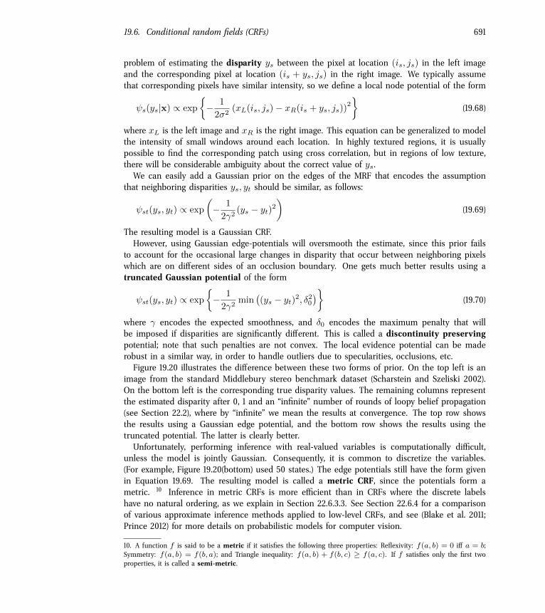
19.6. Conditional random fields (CRFs) 691
problem of estimating the disparity ys between the pixel at location (is, js) in the left imageand the corresponding pixel at location (is + ys, js) in the right image. We typically assumethat corresponding pixels have similar intensity, so we define a local node potential of the form
s(ys|x) / exp
⇢
� 1
2�2
(xL(is, js)� xR(is + ys, js))2
�
(19.68)
where xL is the left image and xR is the right image. This equation can be generalized to modelthe intensity of small windows around each location. In highly textured regions, it is usuallypossible to find the corresponding patch using cross correlation, but in regions of low texture,there will be considerable ambiguity about the correct value of ys.We can easily add a Gaussian prior on the edges of the MRF that encodes the assumption
that neighboring disparities ys, yt should be similar, as follows:
st(ys, yt) / exp
✓
� 1
2�2
(ys � yt)2
◆
(19.69)
The resulting model is a Gaussian CRF.However, using Gaussian edge-potentials will oversmooth the estimate, since this prior fails
to account for the occasional large changes in disparity that occur between neighboring pixelswhich are on di�erent sides of an occlusion boundary. One gets much better results using atruncated Gaussian potential of the form
st(ys, yt) / exp
⇢
� 1
2�2
min
�
(ys � yt)2, �2
0
�
�
(19.70)
where � encodes the expected smoothness, and �0
encodes the maximum penalty that willbe imposed if disparities are significantly di�erent. This is called a discontinuity preservingpotential; note that such penalties are not convex. The local evidence potential can be maderobust in a similar way, in order to handle outliers due to specularities, occlusions, etc.Figure 19.20 illustrates the di�erence between these two forms of prior. On the top left is an
image from the standard Middlebury stereo benchmark dataset (Scharstein and Szeliski 2002).On the bottom left is the corresponding true disparity values. The remaining columns representthe estimated disparity after 0, 1 and an “infinite” number of rounds of loopy belief propagation(see Section 22.2), where by “infinite” we mean the results at convergence. The top row showsthe results using a Gaussian edge potential, and the bottom row shows the results using thetruncated potential. The latter is clearly better.Unfortunately, performing inference with real-valued variables is computationally di�cult,
unless the model is jointly Gaussian. Consequently, it is common to discretize the variables.(For example, Figure 19.20(bottom) used 50 states.) The edge potentials still have the form givenin Equation 19.69. The resulting model is called a metric CRF, since the potentials form ametric. 10 Inference in metric CRFs is more e�cient than in CRFs where the discrete labelshave no natural ordering, as we explain in Section 22.6.3.3. See Section 22.6.4 for a comparisonof various approximate inference methods applied to low-level CRFs, and see (Blake et al. 2011;Prince 2012) for more details on probabilistic models for computer vision.
10. A function f is said to be a metric if it satisfies the following three properties: Reflexivity: f(a, b) = 0 i� a = b;Symmetry: f(a, b) = f(b, a); and Triangle inequality: f(a, b) + f(b, c) � f(a, c). If f satisfies only the first twoproperties, it is called a semi-metric.
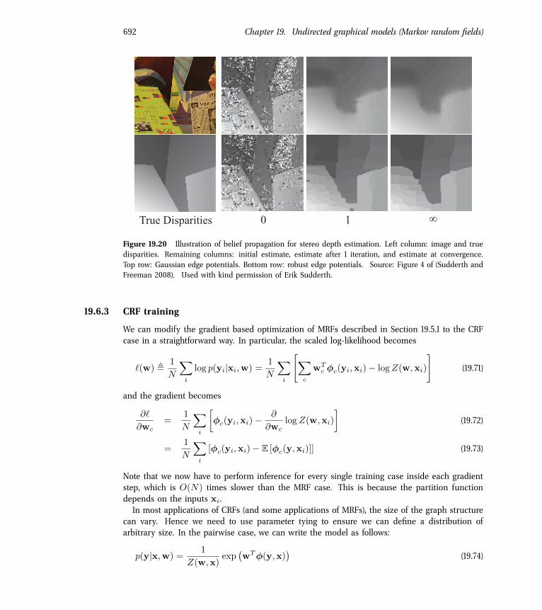
692 Chapter 19. Undirected graphical models (Markov random fields)
0 1True Disparities �
Figure 19.20 Illustration of belief propagation for stereo depth estimation. Left column: image and truedisparities. Remaining columns: initial estimate, estimate after 1 iteration, and estimate at convergence.Top row: Gaussian edge potentials. Bottom row: robust edge potentials. Source: Figure 4 of (Sudderth andFreeman 2008). Used with kind permission of Erik Sudderth.
19.6.3 CRF training
We can modify the gradient based optimization of MRFs described in Section 19.5.1 to the CRFcase in a straightforward way. In particular, the scaled log-likelihood becomes
`(w) , 1
N
X
i
log p(yi|xi,w) =
1
N
X
i
"
X
c
wTc �c(yi,xi)� log Z(w,xi)
#
(19.71)
and the gradient becomes
@`
@wc=
1
N
X
i
�c(yi,xi)� @
@wclog Z(w,xi)
�
(19.72)
=
1
N
X
i
[�c(yi,xi)� E [�c(y,xi)]] (19.73)
Note that we now have to perform inference for every single training case inside each gradientstep, which is O(N) times slower than the MRF case. This is because the partition functiondepends on the inputs xi.In most applications of CRFs (and some applications of MRFs), the size of the graph structure
can vary. Hence we need to use parameter tying to ensure we can define a distribution ofarbitrary size. In the pairwise case, we can write the model as follows:
p(y|x,w) =
1
Z(w,x)
exp
�
wT�(y,x)
�
(19.74)
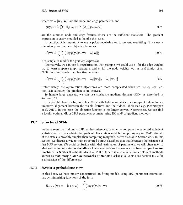
19.7. Structural SVMs 693
where w = [wn,we] are the node and edge parameters, and
�(y,x) , [
X
t
�t(yt,x),X
s⇠t
�st(ys, yt,x)] (19.75)
are the summed node and edge features (these are the su�cient statistics). The gradientexpression is easily modified to handle this case.In practice, it is important to use a prior/ regularization to prevent overfitting. If we use a
Gaussian prior, the new objective becomes
`0(w) , 1
N
X
i
log p(yi|xi,w)� �||w||22
(19.76)
It is simple to modify the gradient expression.Alternatively, we can use `
1
regularization. For example, we could use `1
for the edge weightswe to learn a sparse graph structure, and `
2
for the node weights wn, as in (Schmidt et al.2008). In other words, the objective becomes
`0(w) , 1
N
X
i
log p(yi|xi,w)� �1
||we||1 � �2
||wn||22
(19.77)
Unfortunately, the optimization algorithms are more complicated when we use `1
(see Sec-tion 13.4), although the problem is still convex.To handle large datasets, we can use stochastic gradient descent (SGD), as described in
Section 8.5.2.It is possible (and useful) to define CRFs with hidden variables, for example to allow for an
unknown alignment between the visible features and the hidden labels (see e.g., (Schnitzspanet al. 2010)). In this case, the objective function is no longer convex. Nevertheless, we can finda locally optimal ML or MAP parameter estimate using EM and/ or gradient methods.
19.7 Structural SVMs
We have seen that training a CRF requires inference, in order to compute the expected su�cientstatistics needed to evaluate the gradient. For certain models, computing a joint MAP estimateof the states is provably simpler than computing marginals, as we discuss in Section 22.6. In thissection, we discuss a way to train structured output classifiers that that leverages the existence offast MAP solvers. (To avoid confusion with MAP estimation of parameters, we will often refer toMAP estimation of states as decoding.) These methods are known as structural support vectormachines or SSVMs (Tsochantaridis et al. 2005). (There is also a very similar class of methodsknown as max margin Markov networks or M3nets (Taskar et al. 2003); see Section 19.7.2 fora discussion of the di�erences.)
19.7.1 SSVMs: a probabilistic view
In this book, we have mostly concentrated on fitting models using MAP parameter estimation,i.e., by minimizing functions of the form
RMAP (w) = � log p(w)�NX
i=1
log p(yi|xi,w) (19.78)
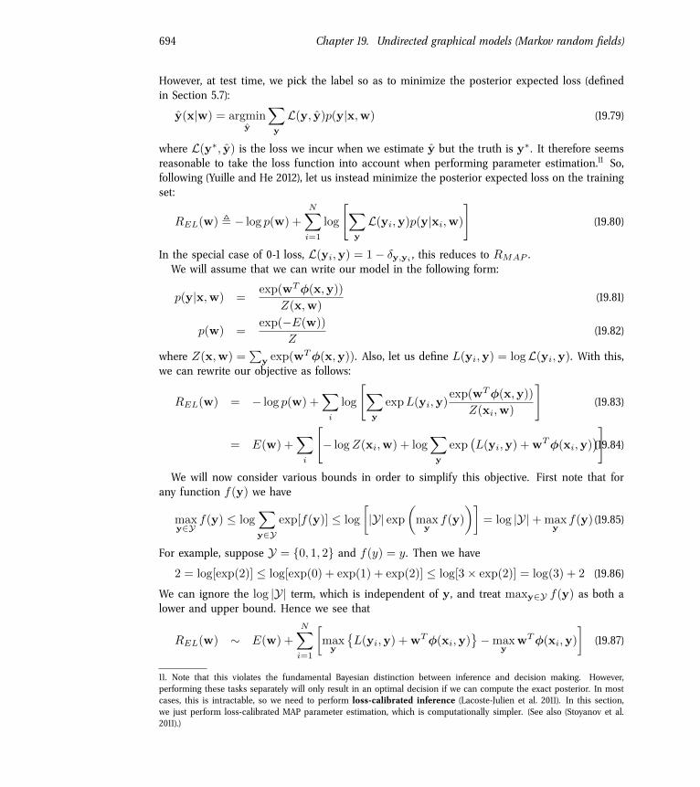
694 Chapter 19. Undirected graphical models (Markov random fields)
However, at test time, we pick the label so as to minimize the posterior expected loss (definedin Section 5.7):
ˆy(x|w) = argmin
ˆy
X
y
L(y, ˆy)p(y|x,w) (19.79)
where L(y⇤, ˆy) is the loss we incur when we estimate ˆy but the truth is y⇤. It therefore seemsreasonable to take the loss function into account when performing parameter estimation.11 So,following (Yuille and He 2012), let us instead minimize the posterior expected loss on the trainingset:
REL(w) , � log p(w) +
NX
i=1
log
"
X
y
L(yi,y)p(y|xi,w)
#
(19.80)
In the special case of 0-1 loss, L(yi,y) = 1� �y,y
i
, this reduces to RMAP .We will assume that we can write our model in the following form:
p(y|x,w) =
exp(wT�(x,y))
Z(x,w)
(19.81)
p(w) =
exp(�E(w))
Z(19.82)
where Z(x,w) =
P
y
exp(wT�(x,y)). Also, let us define L(yi,y) = log L(yi,y). With this,we can rewrite our objective as follows:
REL(w) = � log p(w) +
X
i
log
"
X
y
exp L(yi,y)
exp(wT�(x,y))
Z(xi,w)
#
(19.83)
= E(w) +
X
i
"
� log Z(xi,w) + log
X
y
exp
�
L(yi,y) + wT�(xi,y)
�
#
(19.84)
We will now consider various bounds in order to simplify this objective. First note that forany function f(y) we have
max
y2Yf(y) log
X
y2Yexp[f(y)] log
|Y| exp
✓
max
y
f(y)
◆�
= log |Y| + max
y
f(y) (19.85)
For example, suppose Y = {0, 1, 2} and f(y) = y. Then we have
2 = log[exp(2)] log[exp(0) + exp(1) + exp(2)] log[3⇥ exp(2)] = log(3) + 2 (19.86)
We can ignore the log |Y| term, which is independent of y, and treat max
y2Y f(y) as both alower and upper bound. Hence we see that
REL(w) ⇠ E(w) +
NX
i=1
max
y
�
L(yi,y) + wT�(xi,y)
�max
y
wT�(xi,y)
�
(19.87)
11. Note that this violates the fundamental Bayesian distinction between inference and decision making. However,performing these tasks separately will only result in an optimal decision if we can compute the exact posterior. In mostcases, this is intractable, so we need to perform loss-calibrated inference (Lacoste-Julien et al. 2011). In this section,we just perform loss-calibrated MAP parameter estimation, which is computationally simpler. (See also (Stoyanov et al.2011).)
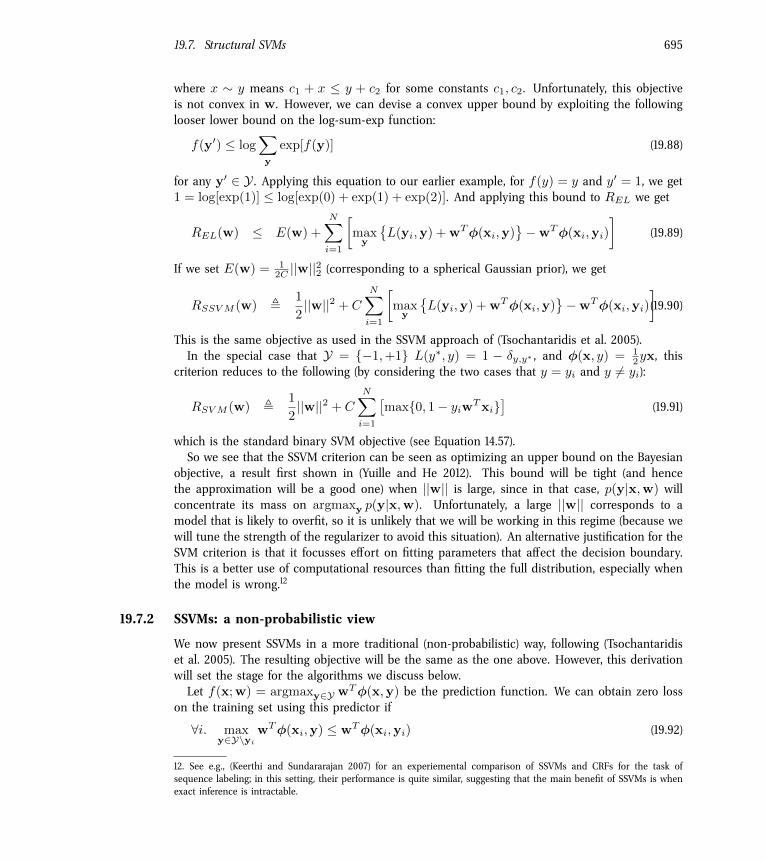
19.7. Structural SVMs 695
where x ⇠ y means c1
+ x y + c2
for some constants c1
, c2
. Unfortunately, this objectiveis not convex in w. However, we can devise a convex upper bound by exploiting the followinglooser lower bound on the log-sum-exp function:
f(y0) log
X
y
exp[f(y)] (19.88)
for any y0 2 Y . Applying this equation to our earlier example, for f(y) = y and y0= 1, we get
1 = log[exp(1)] log[exp(0) + exp(1) + exp(2)]. And applying this bound to REL we get
REL(w) E(w) +
NX
i=1
max
y
�
L(yi,y) + wT�(xi,y)
�wT�(xi,yi)
�
(19.89)
If we set E(w) =
1
2C ||w||22
(corresponding to a spherical Gaussian prior), we get
RSSV M (w) , 1
2
||w||2 + CNX
i=1
max
y
�
L(yi,y) + wT�(xi,y)
�wT�(xi,yi)
�
(19.90)
This is the same objective as used in the SSVM approach of (Tsochantaridis et al. 2005).In the special case that Y = {�1, +1} L(y⇤, y) = 1 � �y,y⇤ , and �(x, y) =
1
2
yx, thiscriterion reduces to the following (by considering the two cases that y = yi and y 6= yi):
RSV M (w) , 1
2
||w||2 + CNX
i=1
⇥
max{0, 1� yiwT xi}
⇤
(19.91)
which is the standard binary SVM objective (see Equation 14.57).So we see that the SSVM criterion can be seen as optimizing an upper bound on the Bayesian
objective, a result first shown in (Yuille and He 2012). This bound will be tight (and hencethe approximation will be a good one) when ||w|| is large, since in that case, p(y|x,w) willconcentrate its mass on argmax
y
p(y|x,w). Unfortunately, a large ||w|| corresponds to amodel that is likely to overfit, so it is unlikely that we will be working in this regime (because wewill tune the strength of the regularizer to avoid this situation). An alternative justification for theSVM criterion is that it focusses e�ort on fitting parameters that a�ect the decision boundary.This is a better use of computational resources than fitting the full distribution, especially whenthe model is wrong.12
19.7.2 SSVMs: a non-probabilistic view
We now present SSVMs in a more traditional (non-probabilistic) way, following (Tsochantaridiset al. 2005). The resulting objective will be the same as the one above. However, this derivationwill set the stage for the algorithms we discuss below.Let f(x;w) = argmax
y2Y wT�(x,y) be the prediction function. We can obtain zero losson the training set using this predictor if
8i. max
y2Y\yi
wT�(xi,y) wT�(xi,yi) (19.92)
12. See e.g., (Keerthi and Sundararajan 2007) for an experiemental comparison of SSVMs and CRFs for the task ofsequence labeling; in this setting, their performance is quite similar, suggesting that the main benefit of SSVMs is whenexact inference is intractable.
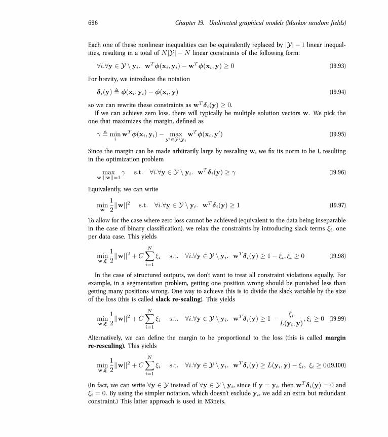
696 Chapter 19. Undirected graphical models (Markov random fields)
Each one of these nonlinear inequalities can be equivalently replaced by |Y|� 1 linear inequal-ities, resulting in a total of N |Y|�N linear constraints of the following form:
8i.8y 2 Y \ yi. wT�(xi,yi)�wT�(xi,y) � 0 (19.93)
For brevity, we introduce the notation
�i(y) , �(xi,yi)� �(xi,y) (19.94)
so we can rewrite these constraints as wT �i(y) � 0.If we can achieve zero loss, there will typically be multiple solution vectors w. We pick the
one that maximizes the margin, defined as
� , min
iwT�(xi,yi)� max
y
02Y\yi
wT�(xi,y0) (19.95)
Since the margin can be made arbitrarily large by rescaling w, we fix its norm to be 1, resultingin the optimization problem
max
w:||w||=1
� s.t. 8i.8y 2 Y \ yi. wT �i(y) � � (19.96)
Equivalently, we can write
min
w
1
2
||w||2 s.t. 8i.8y 2 Y \ yi. wT �i(y) � 1 (19.97)
To allow for the case where zero loss cannot be achieved (equivalent to the data being inseparablein the case of binary classification), we relax the constraints by introducing slack terms ⇠i, oneper data case. This yields
min
w,⇠
1
2
||w||2 + CNX
i=1
⇠i s.t. 8i.8y 2 Y \ yi. wT �i(y) � 1� ⇠i, ⇠i � 0 (19.98)
In the case of structured outputs, we don’t want to treat all constraint violations equally. Forexample, in a segmentation problem, getting one position wrong should be punished less thangetting many positions wrong. One way to achieve this is to divide the slack variable by the sizeof the loss (this is called slack re-scaling). This yields
min
w,⇠
1
2
||w||2 + CNX
i=1
⇠i s.t. 8i.8y 2 Y \ yi. wT �i(y) � 1� ⇠iL(yi,y)
, ⇠i � 0 (19.99)
Alternatively, we can define the margin to be proportional to the loss (this is called marginre-rescaling). This yields
min
w,⇠
1
2
||w||2 + CNX
i=1
⇠i s.t. 8i.8y 2 Y \ yi. wT �i(y) � L(yi,y)� ⇠i, ⇠i � 0 (19.100)
(In fact, we can write 8y 2 Y instead of 8y 2 Y \ yi, since if y = yi, then wT �i(y) = 0 and⇠i = 0. By using the simpler notation, which doesn’t exclude yi, we add an extra but redundantconstraint.) This latter approach is used in M3nets.
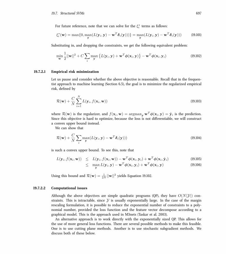
19.7. Structural SVMs 697
For future reference, note that we can solve for the ⇠⇤i terms as follows:
⇠⇤i (w) = max{0, max
y
(L(yi,y)�wT �i(y)))} = max
y
(L(yi,y)�wT �i(y))) (19.101)
Substituting in, and dropping the constraints, we get the following equivalent problem:
min
w
1
2
||w||2 + CX
i
max
y
�
L(yi,y) + wT�(xi,y)
�wT�(xi,yi) (19.102)
19.7.2.1 Empirical risk minimization
Let us pause and consider whether the above objective is reasonable. Recall that in the frequen-tist approach to machine learning (Section 6.5), the goal is to minimize the regularized empiricalrisk, defined by
R(w) +
C
N
NX
i=1
L(yi, f(xi,w)) (19.103)
where R(w) is the regularizer, and f(xi,w) = argmax
y
wT�(xi,y) =
ˆyi is the prediction.Since this objective is hard to optimize, because the loss is not di�erentiable, we will constructa convex upper bound instead.We can show that
R(w) +
C
N
X
i
max
y
(L(yi,y)�wT �i(y))) (19.104)
is such a convex upper bound. To see this, note that
L(yi, f(xi,w)) L(yi, f(xi,w))�wT�(xi,yi) + wT�(xi, ˆyi) (19.105)
max
y
L(yi,y)�wT�(xi,yi) + wT�(xi,y) (19.106)
Using this bound and R(w) =
1
2N ||w||2 yields Equation 19.102.
19.7.2.2 Computational issues
Although the above objectives are simple quadratic programs (QP), they have O(N |Y|) con-straints. This is intractable, since Y is usually exponentially large. In the case of the marginrescaling formulation, it is possible to reduce the exponential number of constraints to a poly-nomial number, provided the loss function and the feature vector decompose according to agraphical model. This is the approach used in M3nets (Taskar et al. 2003).An alternative approach is to work directly with the exponentially sized QP. This allows for
the use of more general loss functions. There are several possible methods to make this feasible.One is to use cutting plane methods. Another is to use stochastic subgradient methods. Wediscuss both of these below.
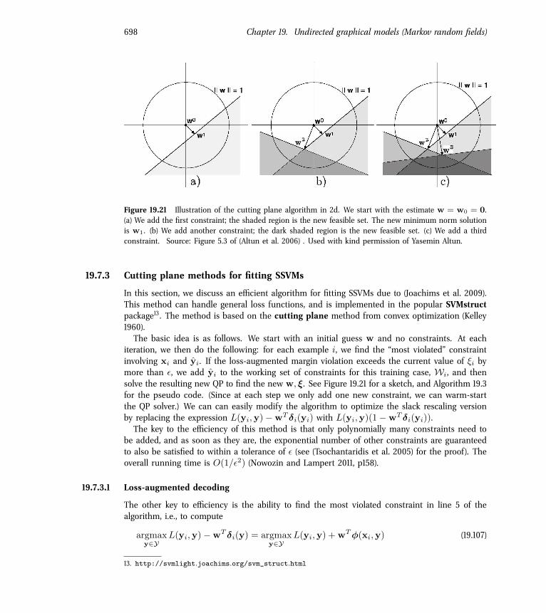
698 Chapter 19. Undirected graphical models (Markov random fields)
2006/08/03 14:15
12 SVM Learning for Interdependent and Structured Output Spaces
Figure 1.3 Cutting plane algorithm. Successive steps of the cutting plane algorithm. In
first step no constraints have been added (no shading), w0
= 0 is the current solution. (a)
Second step: The (potentially) most violated constraint has been added. It cuts o� the
current solution w0
from the feasible region (shaded).(b) Third step: One more violated
constraint is added, and the new solution is computed. (c) Fourth step: The process is
repeated until there are no more violating constraints.
Chow, 1990). In cases where �(yi, ·) only takes on a finite number of values, a
generic strategy is a two stage approach, where one first computes the maximum
over those y for which the cost �(yi,y) is constant, and then maximizes over
the finite number of levels. However, this strategy can scale the computational
complexity by the size of y (e. g. when the cost is the Hamming loss). We now
present the recursion rules of a simple modification of the DP algorithms to compute
(1.16) for Hamming loss and 1 � F1
score. The resulting algorithms are as e�cient
as the original DP algorithm (up to a small constant). This approach can easily be
generalized to any cost function that decomposes into factors that are linear in the
cost of subcomponents of y.
Note that Hamming loss is given by �(y, ¯y) =
PTt=1
¯�(yt, yt), where yt
denotes
the tth component of y (e. g. tth position in a sequence of length T ) and
¯�(a, b) is
0 is a = b and 1 otherwise. Let c(t, �, �0;w) be the local contribution of assigning
� to the tth component with respect to w given the previous variable assignments
�0. Suppressing the dependence on yi
and w, the recursive rules are given by
St(�) = max
�0
�
St�1
(�0) +
¯�(yti , �)Ft�1
(�0) + c(t, �, �0
)[Dt�1
(�0) +
¯�(yti , �)]
�
At(�) = argmax
�0
�
Tt�1
(�0) +
¯�(yti , �)Ft�1
(�0) + c(t, �, �0
)[Dt�1
(�0) +
¯�(yti , �)]
�
Dt(�) = Dt�1
(At(�)) +
¯�(yti , �)
Ft(�) = Ft�1
(At(�)) + c(t, �, At(�)).
where all the variables at t = 0 is 0. Then, the best labeling is achieved by
reconstructing the path from A via argmax� ST (�) in reverse direction.
Note that F1
score, which is the harmonic mean of precision and recall, is
given by �(y, ¯y) = 2a/(p + o), where a is the number of correctly predicted
subcomponents, p is the number of predicted subcomponents and o is the number of
correct subcomponents. Define c such that c(t, �, �0) = 1 if labeling tth component
Figure 19.21 Illustration of the cutting plane algorithm in 2d. We start with the estimate w = w0
= 0.(a) We add the first constraint; the shaded region is the new feasible set. The new minimum norm solutionis w
1
. (b) We add another constraint; the dark shaded region is the new feasible set. (c) We add a thirdconstraint. Source: Figure 5.3 of (Altun et al. 2006) . Used with kind permission of Yasemin Altun.
19.7.3 Cutting plane methods for fitting SSVMs
In this section, we discuss an e�cient algorithm for fitting SSVMs due to (Joachims et al. 2009).This method can handle general loss functions, and is implemented in the popular SVMstructpackage13. The method is based on the cutting plane method from convex optimization (Kelley1960).The basic idea is as follows. We start with an initial guess w and no constraints. At each
iteration, we then do the following: for each example i, we find the “most violated” constraintinvolving xi and ˆyi. If the loss-augmented margin violation exceeds the current value of ⇠i bymore than ✏, we add ˆyi to the working set of constraints for this training case, Wi, and thensolve the resulting new QP to find the new w, ⇠. See Figure 19.21 for a sketch, and Algorithm 19.3for the pseudo code. (Since at each step we only add one new constraint, we can warm-startthe QP solver.) We can can easily modify the algorithm to optimize the slack rescaling versionby replacing the expression L(yi,y)�wT �i(yi) with L(yi,y)(1�wT �i(yi)).The key to the e�ciency of this method is that only polynomially many constraints need to
be added, and as soon as they are, the exponential number of other constraints are guaranteedto also be satisfied to within a tolerance of ✏ (see (Tsochantaridis et al. 2005) for the proof). Theoverall running time is O(1/✏2) (Nowozin and Lampert 2011, p158).
19.7.3.1 Loss-augmented decoding
The other key to e�ciency is the ability to find the most violated constraint in line 5 of thealgorithm, i.e., to compute
argmax
y2YL(yi,y)�wT �i(y) = argmax
y2YL(yi,y) + wT�(xi,y) (19.107)
13. http://svmlight.joachims.org/svm_struct.html
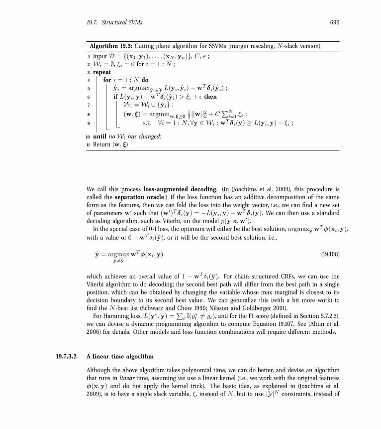
19.7. Structural SVMs 699
Algorithm 19.3: Cutting plane algorithm for SSVMs (margin rescaling, N -slack version)
1 Input D = {(x1
,y1
), . . . , (xN ,yn)}, C , ✏ ;2 Wi = ;, ⇠i = 0 for i = 1 : N ;3 repeat4 for i = 1 : N do5 ˆyi = argmax
ˆy
i
2Y L(yi, ˆyi)�wT �i(ˆyi) ;6 if L(yi,y)�wT �i(ˆyi) > ⇠i + ✏ then7 Wi = Wi [ {ˆyi} ;
8 (w, ⇠) = argmin
w,⇠�0
1
2
||w||22
+ CPN
i=1
⇠i ;9 s.t. 8i = 1 : N, 8y 2Wi : wT �i(y) � L(yi,y)� ⇠i ;10 until no Wi has changed;11 Return (w, ⇠)
We call this process loss-augmented decoding. (In (Joachims et al. 2009), this procedure iscalled the separation oracle.) If the loss function has an additive decomposition of the sameform as the features, then we can fold the loss into the weight vector, i.e., we can find a new setof parameters w0 such that (w0
)
T �i(y) = �L(yi,y) + wT �i(y). We can then use a standarddecoding algorithm, such as Viterbi, on the model p(y|x,w0
).In the special case of 0-1 loss, the optimum will either be the best solution, argmax
y
wT�(xi,y),with a value of 0�wT �i(ˆy), or it will be the second best solution, i.e.,
˜y = argmax
y 6=ˆy
wT�(xi,y) (19.108)
which achieves an overall value of 1 � wT �i(˜y). For chain structured CRFs, we can use theViterbi algorithm to do decoding; the second best path will di�er from the best path in a singleposition, which can be obtained by changing the variable whose max marginal is closest to itsdecision boundary to its second best value. We can generalize this (with a bit more work) tofind the N -best list (Schwarz and Chow 1990; Nilsson and Goldberger 2001).For Hamming loss, L(y⇤,y) =
P
t I(y⇤t 6= yt), and for the F1 score (defined in Section 5.7.2.3),
we can devise a dynamic programming algorithm to compute Equation 19.107. See (Altun et al.2006) for details. Other models and loss function combinations will require di�erent methods.
19.7.3.2 A linear time algorithm
Although the above algorithm takes polynomial time, we can do better, and devise an algorithmthat runs in linear time, assuming we use a linear kernel (i.e., we work with the original features�(x,y) and do not apply the kernel trick). The basic idea, as explained in (Joachims et al.2009), is to have a single slack variable, ⇠, instead of N , but to use |Y|N constraints, instead of

700 Chapter 19. Undirected graphical models (Markov random fields)
just N |Y|. Specifically, we optimize the following (assuming the margin rescaling formulation):
min
w,⇠�0
1
2
||w||22
+ C⇠
s.t. 8(y1
, . . . ,yN ) 2 YN:
1
NwT
NX
i=1
�i(yi) �1
N
NX
i=1
L(yi,yi)� ⇠ (19.109)
Compare this to the original version, which was
min
w,⇠�0
1
2
||w||22
+
C
N
NX
i=1
⇠i s.t. 8i = 1 : N, 8y 2 Y : wT �i(yi) � L(yi,yi)� ⇠i (19.110)
One can show that any solution w⇤ of Equation 19.109 is also a solution of Equation 19.110 andvice versa, with ⇠⇤
=
1
N
PNi=1
⇠⇤i .
Algorithm 19.4: Cutting plane algorithm for SSVMs (margin rescaling, 1-slack version)
1 Input D = {(x1
,y1
), . . . , (xN ,yn)}, C , ✏ ;2 W = ;;3 repeat4 (w, ⇠) = argmin
w,⇠�0
1
2
||w||22
+ C⇠ ;
5 s.t. 8(y1
, . . . ,yN ) 2W :
1
N wTPN
i=1
�i(yi) � 1
N
PNi=1
L(yi,yi)� ⇠;6 for i = 1 : N do7 ˆyi = argmax
ˆy
i
2Y L(yi, ˆyi) + wT�(xi, ˆyi)
8 W = W [ {(
ˆy1
, . . . , ˆyN )};9 until 1
N
PNi=1
L(yi, ˆyi)� 1
N wTPN
i=1
�i(ˆyi) ⇠ + ✏;10 Return (w, ⇠)
We can optimize Equation 19.109 using the cutting plane algorithm in Algorithm 19.4. (Thisis what is implemented in SVMstruct.) The inner QP in line 4 can be solved in O(N) timeusing the method of (Joachims 2006). In line 7 we make N calls to the loss-augmented decoder.Finally, it can be shown that the number of iterations is independent of N . Thus the overallrunning time is linear.
19.7.4 Online algorithms for fitting SSVMs
Although the cutting plane algorithm can be made to run in time linear in the number of datapoints, that can still be slow if we have a large dataset. In such cases, it is preferable to useonline learning. We briefly mention a few possible algorithms below.
19.7.4.1 The structured perceptron algorithm
A very simple algorithm for fitting SSVMs is the structured perceptron algorithm (Collins2002). This method is an extension of the regular perceptron algorithm of Section 8.5.4. At each
19.7. Structural SVMs 701
step, we compute ˆy = argmax p(y|x) (e.g., using the Viterbi algorithm) for the current trainingsample x. If ˆy = y, we do nothing, otherwise we update the weight vector using
wk+1
= wk + �(y,x)� �(
ˆy,x) (19.111)
To get good performance, it is necessary to average the parameters over the last few updates(see Section 8.5.2 for details), rather than using the most recent value.
19.7.4.2 Stochastic subgradient descent
The disadvantage of the structured perceptron algorithm is that it implicitly assumes 0-1 loss,and it does not enforce any kind of margin. An alternative approach is to perform stochasticsubgradient descent. A specific instance of this is the Pegasos algorithm (Shalev-Shwartz et al.2007), which stands for “primal estimated sub-gradient solver for SVM”. Pegasos was designedfor binary SVMs, but can be extended to SSVMS.Let us start by considering the objective function:
f(w) =
NX
i=1
max
ˆy
i
⇥
L(yi, ˆyi) + wT�(xi, ˆyi)⇤�wT�(xi,yi) + �||w||2 (19.112)
Letting ˆyi be the argmax of this max. Then the subgradient of this objective function is
g(w) =
NX
i=1
�(xi, ˆyi)� �(xi,yi) + 2�w (19.113)
In stochastic subgradient descent, we approximate this gradient with a single term, i, and thenperform an update:
wk+1
= wk � ⌘kgi(wk) = wk � ⌘k[�(xi, ˆyi)� �(xi,yi) + (2/N)�w] (19.114)
where ⌘k is the step size parameter, which should satisfy the Robbins-Monro conditions (Sec-tion 8.5.2.1). (Notice that the perceptron algorithm is just a special case where � = 0 and⌘k = 1.) To ensure that w has unit norm, we can project it onto the `
2
ball after each update.
19.7.5 Latent structural SVMs
In many applications of interest, we have latent or hidden variables h. For example, in objectdetections problems, we may know that an object is present in an image patch, but not knowwhere the parts are located (see e.g., (Felzenszwalb et al. 2010)). Or in machine translation, wemay know the source text x (say English) and the target text y (say French), but we typically donot know the alignment between the words.We will extend our model as follows, to get a latent CRF:
p(y,h|x,w) =
exp(wT�(x,y,h))
Z(x,w)
(19.115)
Z(x,w) =
X
y,h
exp(wT�(x,y,h)) (19.116)
702 Chapter 19. Undirected graphical models (Markov random fields)
In addition, we introduce the loss function L(y⇤,y,h); this measures the loss when the “action”that we take is to predict y using latent variables h. (As before, we define L(y⇤,y,h) =
log L(y⇤,y,h).) We could just use L(y⇤,y) as before, since h is usually a nuisance variableand not of direct interest. However, h can sometimes play a useful role in defining a lossfunction.14
Given the loss function, we define our objective as
REL(w) = � log p(w) +
X
i
log
2
4
X
y,h
exp L(yi,y,h)
exp(wT�(x,y,h))
Z(x,w)
3
5 (19.117)
Using the same loose lower bound as before, we get
REL(w) E(w) +
NX
i=1
max
y,h
�
L(yi,y,h) + wT�(xi,y,h)
�NX
i=1
max
h
wT�(xi,yi,h) (19.118)
If we set E(w) = � 1
2C ||w||22
, we get the same objective as is optimized in latent SVMs (Yuand Joachims 2009).Unfortunately, this objective is no longer convex. However, it is a di�erence of convex
functions, and hence can be solved e�ciently using the CCCP or concave-convex procedure(Yuille and Rangarajan 2003). This is a method for minimizing functions of the form f(w) �g(w), where f and g are convex. The method alternates between finding a linear upper boundu on �g, and then minimizing the convex function f(w) + u(w); see Algorithm 19.5 for thepseudocode. CCCP is guaranteed to decrease the objective at every iteration, and to converge toa local minimum or a saddle point.
Algorithm 19.5: Concave-Convex Procedure (CCCP)
1 Set t = 0 and initialize w0
;2 repeat3 Find hyperplane vt such that �g(w) �g(wt) + (w �wt)
T vt for all w ;4 Solve wt+1
= argmin
w
f(w) + wT vt ;5 Set t = t + 1
6 until converged;
14. For example, consider the problem of learning to classify a set of documents as relevant or not to a query. Thatis, given n documents x
1
, . . . ,xn for a single query q, we want to produce a labeling yj 2 {�1, +1}, representingwhether document j is relevant to q or not. Suppose our goal is to maximize the precision at k, which is a metric widelyused in ranking (see Section 9.7.4). We will introduce a latent variable for each document hj representing its degreeof relevance. This corresponds to a latent total ordering, that has to be consistent with the observed partial orderingy. Given this, we can define the following loss function: L(y, ˆy, ˆh) = min{1, n(y)
k} � 1
k
Pkj=1
I(yhj
= 1), wheren(y) is the total number of relevant documents. This loss is essentially just 1 minus the precision@k, except we replace1 with n(y)/k so that the loss will have a minimum of zero. See (Yu and Joachims 2009) for details.
19.7. Structural SVMs 703
When applied to latent SSVMs, CCCP is very similar to (hard) EM. In the “E step”, we computethe linear upper bound by setting vt = �C
PNi=1
�(xi,yi,h⇤i ), where
h⇤i = argmax
h
wTt �(xi,yi,h) (19.119)
In the “M step”, we estimate w using techniques for solving fully visible SSVMs. Specifically, weminimize
1
2
||w||2
+ CNX
i=1
max
y,h
n
˜L(yi,y,h) + wT�(xi,y,h)
o
� CNX
i=1
wT�(xi,yi,h⇤i ) (19.120)
Exercises
Exercise 19.1 Derivative of the log partition function
Derive Equation 19.40.
Exercise 19.2 CI properties of Gaussian graphical models
(Source: Jordan.)
In this question, we study the relationship between sparse matrices and sparse graphs for Gaussiangraphical models. Consider a multivariate Gaussian N (x|µ,⌃) in 3 dimensions. Suppose µ = (0, 0, 0)
T
throughout.
Recall that for jointly Gaussian random variables, we know that Xi and Xj are independent i� they areuncorrelated, ie. ⌃ij = 0. (This is not true in general, or even if Xi and Xj are Gaussian but not jointlyGaussian.) Also, Xi is conditionally independent of Xj given all the other variables i� ⌃�1
ij = 0.
a. Suppose
⌃ =
0
@
0.75 0.5 0.25
0.5 1.0 0.50.25 0.5 0.75
1
A
Are there any marginal independencies amongst X1
, X2
and X3
? What about conditional indepen-dencies? Hint: compute ⌃�1 and expand out xT
⌃
�1x: which pairwise terms xixj are missing? Drawan undirected graphical model that captures as many of these independence statements (marginal andconditional) as possible, but does not make any false independence assertions.
b. Suppose
⌃ =
0
@
2 1 0
1 2 1
0 1 2
1
A
Are there any marginal independencies amongst X1
, X2
and X3
? Are there any conditional inde-pendencies amongst X
1
, X2
and X3
? Draw an undirected graphical model that captures as many ofthese independence statements (marginal and conditional) as possible, but does not make any falseindependence assertions.
c. Now suppose the distribution on X can be represented by the following DAG:
X1
! X2
! X3
704 Chapter 19. Undirected graphical models (Markov random fields)
Let the CPDs be as follows:
P (X1
) = N (X1
; 0, 1), P (X2
|x1
) = N (X2
; x1
, 1), P (X3
|x2
) = N (X3
; x2
, 1) (19.121)
Multiply these 3 CPDs together and complete the square to find the corresponding joint distributionN (X
1:3
|µ,⌃). (You may find it easier to solve for ⌃�1 rather than ⌃.)
d. For the DAG model in the previous question: Are there any marginal independencies amongst X1
, X2
and X3
? What about conditional independencies? Draw an undirected graphical model that capturesas many of these independence statements as possible, but does not make any false independenceassertions (either marginal or conditional).
Exercise 19.3 Independencies in Gaussian graphical models
(Source: MacKay.)
a. Consider the DAG X1 X2 ! X3. Assume that all the CPDs are linear-Gaussian. Which of thefollowing matrices could be the covariance matrix?
A =
0
@
9 3 1
3 9 3
1 3 9
1
A , B =
0
@
8 �3 1
�3 9 �3
1 �3 8
1
A , C =
0
@
9 3 0
3 9 3
0 3 9
1
A , D =
0
@
9 �3 0
�3 10 �3
0 �3 9
1
A(19.122)
b. Which of the above matrices could be inverse covariance matrix?
c. Consider the DAG X1 ! X2 X3. Assume that all the CPDs are linear-Gaussian. Which of theabove matrices could be the covariance matrix?
d. Which of the above matrices could be the inverse covariance matrix?
e. Let three variables x1
, x2
, x4
have covariance matrix ⌃(1:3)
and precision matrix ⌦(1:3)
= ⌃�1
(1:3)
asfollows
⌃(1:3)
=
0
@
1 0.5 0
0.5 1 0.50 0.5 1
1
A ,⌦(1:3)
=
0
@
1.5 �1 0.5�1 2 �1
0.5 �1 1.5
1
A (19.123)
Now focus on x1
and x2
. Which of the following statements about their covariance matrix ⌃(1:2)
andprecision matrix ⌦
(1:2)
are true?
A : ⌃(1:2)
=
✓
1 0.50.5 1
◆
, B : ⌦(1:2)
=
✓
1.5 �1
�1 2
◆
(19.124)
Exercise 19.4 Cost of training MRFs and CRFs
(Source: Koller.) Consider the process of gradient-ascent training for a log-linear model with k features,given a data set with N training instances. Assume for simplicity that the cost of computing a singlefeature over a single instance in our data set is constant, as is the cost of computing the expected valueof each feature once we compute a marginal over the variables in its scope. Assume that it takes c timeto compute all the marginals for each data case. Also, assume that we need r iterations for the gradientprocess to converge.
• Using this notation, what is the time required to train an MRF in big-O notation?
• Using this notation, what is the time required to train a CRF in big-O notation?
19.7. Structural SVMs 705
Exercise 19.5 Full conditional in an Ising model
Consider an Ising model
p(x1
, . . . , xn|✓) =
1
Z(✓)
Y
<ij>
exp(Jijxixj)
nY
i=1
exp(hixi) (19.125)
where < ij > denotes all unique pairs (i.e., all edges), Jij 2 R is the coupling strength (weight) on edgei� j, hi 2 R is the local evidence (bias term), and ✓ = (J,h) are all the parameters.
If xi 2 {0, 1}, derive an expression for the full conditional
p(xi = 1|x�i, ✓) = p(xi = 1|xnbi
, ✓) (19.126)
where x�i are all nodes except i, and nbi are the neighbors of i in the graph. Hint: you answer shoulduse the sigmoid/ logistic function �(z) = 1/(1 + e�z
). Now suppose xi 2 {�1, +1}. Derive a relatedexpression for p(xi|x�i, ✓) in this case. (This result can be used when applying Gibbs sampling to themodel.)
Related Documents