18A. 1 THE CANOPY HORIZONTAL ARRAY TURBULENCE STUDY (CHATS)

18A.1 THE CANOPY HORIZONTAL ARRAY TURBULENCE STUDY (CHATS)

Edward G. Patton1∗, Thomas W. Horst1, Donald H. Lenschow1, Peter P. Sullivan1,Steven Oncley1, Sean Burns1, Alex Guenther1, Andreas Held1, Thomas Karl1, Shane Mayor1,

Luciana Rizzo1, Scott Spuler1, Jielun Sun1, Andrew Turnipseed1, Eugene Allwine2,Steven Edburg2, Brian Lamb2, Roni Avissar3, Heidi E. Holder3, Ron Calhoun4,

Jan Kleissl5, William Massman6, Kyaw Tha Paw U7, Jeffrey C. Weil8

1National Center for Atmospheric Research, Boulder, CO2Washington State University, Pullman, WA

3Duke University, Durham, NC4Arizona State University, Tempe, AZ

5University of California, San Diego, CA6USDA Forest Service, Fort Collins, CO

7University of California, Davis, CA8University of Colorado, Boulder, CO

1. MOTIVATION

1.1 Turbulent exchange within and above tall vege-tation

Turbulence in the planetary boundary layer (PBL) wellabove the surface has been shown to be independent ofthe details of the surface roughness. In this region well-quantified similarity relationships work well when char-acterizing turbulent fluxes (e.g.,Raupach, 1979). How-ever, in the near-surface layer which is directly influ-enced by roughness elements,i.e., the roughness sub-layer, turbulence exhibits dramatically varying proper-ties depending on the detailed structure of the roughnesselements (Shaw et al., 1974; Raupach, 1981; Raupachet al., 1996). Turbulence in the roughness sublayer islargely responsible for transporting momentum, heat andscalars between the surface and the flow aloft, and is di-rectly coupled with the overlying larger-scale turbulence.Therefore, accurate characterization of fluxes within theroughness sublayer is crucial for predicting larger-scaleatmospheric flow and scalar transport.

Tall plant canopies cover about 30% of the Earth’sland surface and are particularly complex roughnessstructures because of their seasonal variability, flexibil-ity, and porosity. Furthermore, leaves and branches oc-cur in both random and organized distributions within thecanopy. Spectra and co-spectra are more sharply peakedfor canopy flow than for flow over smooth walls (Shawet al., 1974; Finnigan, 1979a; Raupach et al., 1986). Nearthe canopy top, longitudinal and vertical velocity per-

∗Corresponding address:Edward G. Patton, National Center forAtmospheric Research, P. O. Box 3000, Boulder, CO, 80307-3000. E-mail: [email protected]

turbations are more strongly correlated than aloft (Rau-pach, 1981), implying more efficient momentum trans-port than in the rest of the PBL. Observations have shownthat the turbulence here is highly intermittent and domi-nated in daytime by cool-air downbursts (sweeps) (Finni-gan, 1979b; Shaw et al., 1983; Denmead and Bradley,1985; Baldocchi and Meyers, 1988). Gao et al. (1989)documented the sloping sharp interface between the ris-ing warm air from the canopy (ejections) and sweeps,and determined that these organized motions are respon-sible for 60–80% of the fluxes of momentum, energyand scalars within and above the canopy. Raupach et al.(1996) postulated that these structures might be roll vor-tices generated by the shear induced by the drag of theplant canopy.

The ground and the vegetation may serve as either ascalar source or sink; sometimes one may be a sourceand the other a sink. Species can also chemically re-act on time scales that affect their transport within andabove the canopy (Patton et al., 2001). The distribu-tion of canopy sources/sinks depends on the amount andstate of the canopy foliage, which varies throughout theseasonal cycle for deciduous trees; from bare limbs inwinter (no photosynthesis and an open canopy) to rapidgrowth in spring (increasing photosynthesis and canopydensity), to maturity in summer (more constant photo-synthesis and canopy density), to senescence and leaf-drop in fall (decreasing photosynthesis and canopy den-sity). Thus, a broad spectrum of different conditions oc-curs through the year, and both dynamical and scalarfluxes exhibit height dependence and seasonal variabil-ity.

1.2 Linking models and measurements

Large-eddy simulation (LES) is one of the best avail-able tools capable of linking turbulent motions withscales ranging from the microscale to the mesoscale.Using a three-dimensional grid, LES solves the time-dependent filtered Navier-Stokes equations to predict allresolved scales of motion as they evolve in space andtime while using a subfilter-scale (SFS) model to param-eterize only the smallest scales. An important compo-nent of LES is that active, passive and reactive scalarscan all be incorporated depending on the topic of inter-est. As numerical techniques and computational capabil-ities have improved over the last thirty years, LES resultshave become a direct counterpart to measurements.

An intriguing aspect of canopy-resolving LES is thatbecause of the canopy-imposed length scale (i.e., thecanopy height) increased grid resolution can improve theaccuracy of the simulation. Whereas increased resolu-tion in simulations over bare ground continually reducesthe scale of the peak in the vertical velocity energy spec-trum.

1.3 Previous SFS campaigns

Despite its myriad contributions to understanding tur-bulent flows, LES does have shortcomings and needs tobe validated and improved to deal with complex flows,especially for surface layers where dependence on theSFS model increases. To address this issue, NCARin collaboration with several university groups recentlycarried out two pioneering observational studies to im-prove subfilter-scale parameterizations over flat terrainwith sparse low-lying vegetation (Horizontal Array Tur-bulence Study, HATS) and over the ocean (Ocean HATS;OHATS) (e.g.,Sullivan et al., 2003, Horst et al., 2004).These studies applied a technique first proposed by Tonget al. (1998) that uses horizontal arrays of 14 to 18sonic anemometers/thermometers deployed at two levelsto measure spatially filtered variables and their gradientswhich appear in the equations of motion. These datasetshave provided an observational basis for validating anddeveloping closure approximations.

1.4 Canopy influence on SFS motions

Vegetation dramatically complicates the effects ofSFS motions. Canopy elements are distributed spa-tially, thereby spreading sources/sinks of momentum andscalars throughout the canopy layer. The elements alsotend to occur in clumps. Large-scale turbulence (largerthan the scale of the clumping) interacting with theseclumped elements can rapidly break down into smallerwake-scale motions thereby short-circuiting the inertialenergy cascade. In addition, depending on the density of

the canopy elements, the spatially-distributed plant struc-tures intercept (and are heated by) solar radiation dur-ing daytime and radiatively cool faster than the surfaceat night. As a result, in daytime (nighttime) they can cre-ate stable (unstable) conditions within and beneath thecanopy when the overlying atmosphere is unstably (sta-bly) stratified.

To parameterize SFS fluxes, canopy-LES currently as-sumes that the SFS motions occur within the inertialsubrange and that all wake-scale motions are at a smallenough scale that they immediately dissipate to heat. Re-cently, Shaw and Patton (2003) attempted to improveSFS parameterizations for canopy-resolving LES by al-lowing wake-scale motions to transport turbulence, butin this study the inertial range assumptions were stillrequired. Finnigan (2000) presented an alternative toKolmogorov’s inertial range theory describing the cas-cade of energy from large to small scales which includespressure and viscous drag effects of plants, but this the-ory has not been thoroughly tested. At this point, wedo not know the character of within-canopy SFS mo-tions, nor the role played by eddies shed in the lee ofthe plant elements, nor how these wake-scale motionsaffect scalar and momentum transport. We hypothesizethat spatial variations of the canopy elements modifySFS motions through canopy-induced stratification andscalar/momentum source/sink distributions.

When this experiment was originally proposed, mea-suring arrays of subfilter-scale variables within thecanopy had not been previously attempted, mostly be-cause of the daunting technological challenges and theinterdisciplinary nature of the research. However, re-cently, Zhu et al. (2007) reported an attempt to measureSFS momentum fluxes in a wind-tunnel model canopyusing laser-Doppler velocimetry. Their results lend to theimportance of this work, but are lacking in the ability toassess the impact of vegetation on scalar transport and tocharacterize the impact of the large atmospheric bound-ary layer scales of motion and thermal stratification.

Ultimately, CHATS aims to learn about SFS motionswithin canopies and thereby improve the coupling be-tween canopy-LES and PBL models. This is an impor-tant step in carrying out LES of scalar and momentumtransport in this complex regime, and thus in buildinga unified model of surface-atmospheric exchange in theframework of global and regional land, atmosphere, andchemical models. We also wanted to collect as completeand high-quality a dataset as necessary to be able to test,evaluate and improve one-dimensional column models ofcoupled land-surface/atmosphere exchange.

N C A R R E A L3 0 m T o w e rH o r i z o n t a l A r r a yA S U L I D A R a n dN C A R M i n i �S O D A R / R A S SC i l k e r O r c h a r d s

~ 8 0 0 m

N

Figure 1: Images from Google Earth depicting the location ofCilker Orchards. Upper left image shows the locationof the orchard with respect to Vacaville and Davis, California. Bottom right image shows the location of the variousinstrumentation with respect to Cilker Orchards.

2. THE EXPERIMENT

2.1 The site

With the help and equipment largely from NCAR’s In-Situ Sensing Facility, CHATS took place in one of CilkerOrchard’s walnut blocks in Dixon, California (see Figure1). We chose this location and orchard for many reasons;with the main factors including the size, age, and man-agement practices of the orchard combined with consis-tent wind direction and speed. Figure 1 shows four 800-m-square sections. As depicted, the CHATS instrumen-tation focused on the north-east section. In this section,the trees were all Chandler walnuts. To the south is a mixof slightly younger Chandler and Tulare walnuts. To thewest is a section of mostly Howard walnuts with a smallsection of Tulare in the very north-west corner. The sec-tion to the south-west is a variety of almonds.

The terrain in this part of California’s Central Valleyis flat; less than a 1 m elevation difference across the 1.6km2 orchard block. The elevation at the center of theorchard is about 21 m above sea level.

Twenty-four years of data from the Davis Califor-nia Irrigation Management Information System (CIMIS,http://wwwcimis.water.ca.gov) showed the mean winddirection to be fairly consistent; 50% from the north and50% from the south with a small westerly component.We chose to focus on winds from the south because theCIMIS data also showed that winds from the south tendto be weaker in magnitude with smaller direction vari-ability, providing the potential for sampling a greaterrange of stability. For maximum fetch, the main towerswere located near the northern-most border of the section(see Figure 1).

The campaign took place over twelve weeks whichwas broken into three four-week periods. Intensive mea-

Normalized Leaf Area Density ( a * h )

Nor

mal

ized

Hei

ght

(z

/h)

0 1 2 3 4 5 60

0.2

0.4

0.6

0.8

1

no-leaveswith-leaves

Figure 2: Plant area density profiles measured duringCHATS. These profiles are averaged over measurementstaken throughout each month of intensive operation andare normalized by the canopy height (h). The symbolsrepresent the data, and the lines are parabolic-spline fits.No-leaves: red line with square symbols, With-leaves:green line with triangles.

surements occurred during first four-week period (March15 - April 13) focusing on the walnut trees before leaf-out. Measurements continued through the second four-week period (April 14 - May 13), but the instrumentswere unattended while waiting for the leaves. Intensivemeasurements then continued during the third four-weekperiod (May 13 - June 12) focusing on the impact of theleaves on the fluid mechanics, stability, and source-sinkdistribution of the scalars.

The trees in our section were planted in a nearly-square pattern such that they were about 6.9 m apartin the N-S direction, and 7.3 m in the W-E direction.The trees were all about 25 years old with an averageheight (h) of about ten meters. The horizontal distribu-tion of the vegetation was nearly homogeneous with theexception of an occasional tree that had been lost andre-planted. The vertical plant area density distributionwas measured regularly through the campaign using aLi-Cor LAI-2000. Before leaf-out, the plant area index(PAI) was about 0.7, while following leaf-out the PAI in-creased to about 2.5. Figure 2 shows the average verticalprofile of normalized plant area density both before andafter leaf-out.

2.2 Characterizing the canopy-scales and smaller

Within the orchard, the instrumentation was located intwo main arrangements. Both the horizontal array and

the thirty meter tower were centered within the sectionin the W-E direction; the 30 m tower was located about100 m south from the northern-most edge of the section,and the horizontal array another 100 m south from thetower.

2.2.1 The horizontal array

The towers The horizontal array consisted of five 12m tall towers that were deployed in the W-E direction(across the mean wind). The towers were situated suchthat the three middle towers were each 1.72 m apart withthe middle tower situated immediately within the treerow. The outer two towers were located due west or eastin the adjacent tree rows, about 7 m away. Therefore, theentire array spanned three tree rows (two row middles).

On each of the four outermost towers, rails were at-tached to allow a cart to move vertically on the tow-ers. Two carts were designed and manufactured by theNCAR Earth Observing Facility’s Design and Fabrica-tion Services. Each of these carts consisted basically ofend pieces connecting two horizontal tower sections thatwere separated vertically by one meter. The carts wereattached to ropes and pulleys allowing the carts to be eas-ily raised or lowered to any location from the ground upto the canopy-top or just above. This flexibility facili-tated rapid modification of the instrument arrangementwith minimal impact on normal orchard operations.

The main instrumentation The instrumentation in thehorizontal array consisted largely of two rows of sensorsvertically separated by one meter. The bottom row in-cluded nine CSAT-3 sonic anemometers and five Li-Cor7500 CO2/H2O sensors. The 7500’s were co-locatedwith the central five CSAT-3’s. The top row also in-cluded nine CSAT-3 sonic anemometers, but were com-plemented by five Krypton hygrometers that were alsocollocated with the central five sonic anemometers . Alsoset within the upper five central CSAT-3’s were fiveDantek single-wire hot-film anemometers. These instru-ments were all oriented toward the south on 1.5m booms.

Due to the difficulties in obtaining accurate meantemperature measurements from the sonic anemometers,two NCAR-Vaisala Hygrothermometers (TRH) collectedmean aspirated temperature and relative humidity at 2Hz; one at each level of the array.

The scientific plan During the experiment, the arraywas modified once every five to seven days. These tran-sitions included cart height and horizontal sensor sepa-ration variations. To properly characterize the impact ofleaves on the turbulent momentum and scalar fluxes, werepeated each arrangement during the two phases of theexperiment (i.e.,no-leaves and with-leaves).

Figure 3: Pictures of the array in CHATS. Left: wide-high arrangement with-leaves; upper-right: narrow-high arrange-ment with-leaves; middle-right: wide-high arrangement no-leaves, bottom-right: wide-low arrangement no-leaves.

The two horizontal sensor distributions included twoseparations, 0.5 m and 1.72 m. These spacing were cho-sen such that when using a five-point filter, the filter-scaleseparating resolved and sub-filter scale motions wouldfall at 2 and 6.9 m respectively. The 2 m filter-widthwas chosen because this width is typical of that used incanopy-resolving LES. The 6.9 m spacing was chosenfor a number of reasons. The first is that this was thelargest we could go given the constraints imposed by theorchard operations and the length of the horizontal towersections. The second is that the canopy-imposed elevatedvelocity shear at the top of the vegetation imposes an im-portant length scale on the flow and we wanted to makesure to have at least one filter-width that fell well withinthe energy-containing range of the turbulence and there-fore averaged much of the canopy-induced scales of mo-tion.

In the “narrow” arrangement (0.5 m separation), allthe sensors were located on a single cart and thereforethe sensors spanned between two tree-rows or across asingle row-middle. In the “wide” arrangement (1.72 mseparation), four sensors were located on each level of

each cart, and the middle sensors were located on thecentral tower.

For each of the intensive months, measurements weretaken with the instrumentation configured in six arrange-ments (the narrow and wide horizontal separations ateach of three heights; low - 2.5m , middle - 6m, high- 10.1m). The high location was chosen because it isthe region of highest vertical shear of the streamwise ve-locity and where the majority of the momentum is ex-tracted by the canopy. The middle height was chosenas close as possible to the within-canopy streamwise ve-locity minimum where we expect wake-scale motions tobe extremely important in momentum transport and thepeak in the canopy-imposed scalar source/sink distribu-tion to occur. The low height was chosen to be deepwithin the canopy at a height where the momentum trans-fer was expected to be largely a result of canopy-scalecoherent structures and to be counter-gradient (i.e., thevelocity gradient is positive upward, centered at about2.5 m).

1.5

3.0

4.5

18.0

6.0

11.0

23.0

CS = CSAT3 Sonic Anemometer

HF = Hot-Film Anemometer

P = Fast Pressure

TRH = Temp. / Relative Humidity

K = Krypton Hygrometer

R = 4-Comp. Radiation

PAR = Photosynth. Active Radiation

RC = Reactive Chemistry

A = Aerosol

9.0

14.0

7.5

K

CS

CS

CS

CS

CS

CS

CS

CS

CS

TQ

TQ

TQ

TQ

TQ

TQ

TQ

TQ

TQ

Soil Heat Flux, Soil Moisture, Soil Temperature

Leaf Temperature

Stomatal Conductance

Transpiration

CS TQ

CS TQ 29.0

CS TQ

HF

HF

HF

12.5

10.0

P

K

K

K

K

K

CS

16.0

RC

RC

RC

RC

RC

RC

RC

RC

A

PAR

PAR

PAR

PAR

R

Figure 4: Left: 30 m tower configuration. Numbers on grey tower are in meters. Right: Pictures of the 30m towerfrom below; above: no-leaves, below: with-leaves.

2.2.2 The thirty meter tower

Velocity, temperature and moisture The thirty me-ter tower included thirteen main measurement levels. Toaccurately capture the turbulence in the high velocityshear region near the canopy top, the instruments weretightly focused about this height and growing in separa-tion distance away from this focal point. Six of thesethirteen levels were located below the canopy-top andsix above (see Figure 4 for the actual heights). Each ofthe thirteen primary measurement levels consisted of aCampbell Scientific CSAT-3 sonic anemometer measur-ing all three wind components and virtual temperatureat 60 Hz, and 2) an NCAR-Vaisala Hygrothermometer(TRH) measuring mean aspirated temperature and rela-tive humidity at 2 Hz. At six levels (deployed at every-other level), we sampled specific humidity fluctuationsusing a Campbell Scientific Krypton hygrometer operat-ing at 20 Hz. To maximize the acceptable wind direc-tions, we deployed the sonic anemometers and the Kryp-ton hygrometers on booms that were 1.5m in length and

directed to the west. To minimize their influence on theturbulence measurements, the TRH’s were deployed onsimilar booms pointing to the east.

Mounted to the center of the sonic anemometers andpointed to the south, we installed a Dantek constanttemperature triple-wire hot film anemometer at each ofthree levels (mid canopy 6m, canopy top 10m, and abovecanopy 14m) which were sampling at 2 KHz. These sen-sors will provide direct dissipation measurements as in-fluenced by vegetation.

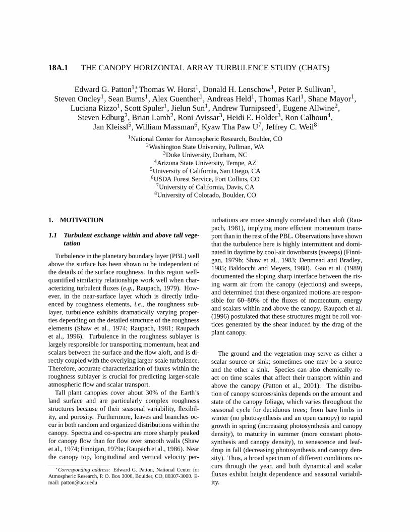
Pressure fluctuations Measurements of turbulentpressure fluctuations (p′) were made during CHATS.Quad-disk probes (Nishiyama and Bedard, Jr., 1991)were used to avoid dynamic pressure errors (Figure 5.Ports made by NOAA/ETL were chosen based on windtunnel testing of three versions of this design. Eventhese ports have errors that change from below 5% toabove 50% as the pitch angle changes from 20 to 30 de-grees. Therefore, use of the ports in the canopy (where

Figure 5: Photograph of the quad-disk pressure portwhen the second pressure port was vertically centeredwithin the array. Also to note in this photograph are thesingle-wire hot film anemometer mounted within the up-per CSAT3 sonic anemometer and the krypton hygrome-ter located behind.

turbulence intensity and thus instantaneous wind attackangles are large) may require that much of the data beused with caution. One port location was placed in thehorizontal array and thus is expected to suffer from thisproblem, however the other was placed at approximately1.1h, where Fitzmaurice et al. (2004) found that turbu-lence intensity has diminished from that found just insidethe canopy.

Two types of sensors were used, one similar to thatdescribed by Wilczak and Bedard, Jr. (2004) that usedan analog transducer and a reference volume with a cal-ibrated leak, and another that used a digital transducerand a fixed reference volume with a large thermal timeconstant. (A third, slower response, sensor also was de-ployed to verify the p′ sensor operation at low frequen-cies.) Before being placed in their final locations, thesystems were connected to the same pressure port anddetermined to be operating properly. Preliminary resultsindicate that the p′ sensors were responding appropri-ately.

For the entire second phase of the experiment, one ofthese pressure ports was shifted into the array. Futurework will be to compare these measurements to canopyflow models and to describe the variation of pressure

transport of TKE at the different heights within and nearthe canopy and to investigate the pressure destructionterm in the filtered scalar flux equation that is modeledin LES.

Radiation For the entire campaign, a two long- andshort-wave Kipp & Zonen radiometers were deployedat 16m to characterize the down-welling and up-wellingfull-spectrum above-canopy radiation. A similar set ofinstruments manufactured by Eppley was deployed twotree rows to the west at a height of 2 m to capture the sub-canopy radiational forcing. A Micromet Systems Q7 netradiometer was also installed at this location to comple-ment the Eppley sub-canopy four-component radiationmeasurements. All radiation measurements were sam-pled at 1 Hz. Two meters from the sub-canopy radiationmeasurements, soil moisture, temperature and heat fluxwere measured at 5cm depth at a rate of 1 Hz.

During the second intensive phase of the experiment,photosynthetically active radiation (PAR) measurementswere taken at four heights (2, 5, 8, and 12 m). The upper-most height was a Li-Cor LI-190 Quantum sensor, whilethe other three levels were Li-Cor LI-191 Line Sensors.

Reactive chemistry Most previous studies have as-sumed negligible chemical effects (either losses or pro-duction) upon the measured eddy fluxes of ozone abovecanopies (for example, see Mikkelsen et al., 2000). How-ever, a recent study implied that up to 50% of the ozonedeposition observed may be explained by fast chem-istry near or within the canopy between ozone and reac-tive volatile organic species that are not easily measured(Kurpius and Goldstein, 2003). The large amount of ver-tical turbulence and flux measurements at CHATS pro-vided an excellent opportunity to study ozone behaviorand chemistry through-out a plant canopy.

We combined gradients from vertical profiles of keytrace gas species (e.g.,O3, NO, NOx) measured at (1.5,4.5, 9, 11, 14, 23)m with disjunct eddy covariance fluxmeasurements of ozone at two levels above the canopy(14 and 23 m) to see if chemistry could be affecting themeasured ozone flux.

These trace gas fluxes were taken at similar heights towater vapor fluxes. Because no chemical effects uponH2O are expected, H2O fluxes serve as a control mea-surement for deducing vertical divergences in the fluxdue to factors other than chemistry. For example, dur-ing southerly flow across the orchard, we would expectonly small vertical divergences in the fluxes of H2O andO3. However, during periods of northerly winds thereis inadequate homogeneous fetch and both H2O and O3

fluxes should exhibit vertical divergences due to differ-ing contributions from the two vegetation types withinthe flux footprints.

The through-canopy concentration profiles can becombined with the vertical turbulence data to providefurther information concerning sources and sinks ofthese trace gases. To this end, we also measured verti-cal concentration profiles of CO2 and H2O in order toascertain the exchange of these passive scalars. Thesespecies have similar surface flux controls (i.e., stomataand soil processes) to the more reactive species such asO3 and NOx. We hope that this study serves as a modelfor our future instrument deployments, integrating fasteddy covariance measurements with canopy profiling inorder to better understand within-canopy processes andtheir impact on measured fluxes.

Gradient measurements of volatile organic com-pounds (VOC) were performed using a Proton-Transfer-Reaction Mass Spectrometer (PTR-MS∗). On 3 days fastmeasurements of selected VOCs were performed on 3levels (4.5m, 9m, 11m). The PTR-MS instrument has atime response (e.g.,10 Hz) suitable for eddy covariancemeasurements (e.g.,10 Hz, see Karl et al., 2000), and hasbeen used extensively for disjunct eddy covariance mea-surements (Rinne et al., 2001; Karl et al., 2002; Ammannet al., 2004; Spirig et al., 2005; Lee et al., 2005). Differ-ent in-canopy dispersion schemes for various VOCs willbe assessed and compared with forward LES model runsto evaluate the emission strength of VOCs emitted by thevegetation.

Surprisingly, and for the first time, high levels (upto 120 pptv) of methyl salicylate [C6H4(HO)COOCH3]were detected in ambient air. PTR-MS mass scans wereconfirmed by gas chromatograph mass spectrometer(GC-MS) analysis. Profile measurements showed a dis-tinct source of methyl salicylate from the canopy. Methylsalicylate activates specific defense genes through thesalicylic acid pathway and is thought to act as a volatilesignaling molecule, when plants are under stress or her-bivorous attack. In conjunction with detail dispersionanalysis available during CHATS these measurementswill put constraints on the biological significance of plantto plant communication in the real atmosphere.

Aerosol measurements - turbulent fluxes and particlesize distribution Particle number concentrations weremeasured with a condensation particle counter (CPC3772, TSI Inc., St. Paul, MN) installed on the 30 mtower. The inlet was mounted adjacent to the 14msonic anemometer. Aerosol data were sampled at 10Hz with an instrument time constant of 0.43 s. Turbu-

∗PTR-MS employs a soft ionization technique which preserves im-portant information of the measured compound reflected in the corre-sponding molecular ion. PTR-MS allows for the quantitative on-linedetection of VOCs down to pptv-level concentrations (Lindinger et al.,1998; Hansel et al., 1995; de Gouw et al., 2003) without any precedingsample treatment.

Figure 6: A photograph of leaf-level measurements be-ing taken with a Li-Cor 6400 system. A cherry-pickerallowed for vertical variations of sunlit- and shaded-leafexchanges to be documented.

lent aerosol number fluxes will be calculated by directeddy covariance, and by simulated relaxed eddy accu-mulation (REA) after investigating the scalar similaritybetween aerosol particles, sonic temperature, water va-por, and trace gases. If these quantities are transportedby eddies similarly efficient throughout the scalar spec-tra, easily accessible quantities such as sonic temperaturemay be used as proxy scalars for turbulence parameteri-zations in future aerosol REA systems, thereby extendingcurrent aerosol flux measurement capabilities.

For additional physical characterization (e.g. identifi-cation of particle formation events, general aerosol bur-den), particle size distributions were measured in the di-ameter range from 10 nm to 2µm using a scanning mo-bility particle sizer (SMPS TSI Inc., St. Paul, MN), acondensation particle counter (CPC 3760 TSI Inc., St.Paul, MN) and an optical particle counter (LASAIR, Par-ticle Measuring Systems, Boulder, CO), sampling belowthe canopy at 2 m AGL. During the day, aerosol con-centrations reached 12,000 particles cm−3, decreasing to3,000 particles cm−3 at nighttime.

2.2.3 Leaf-level measurements

Enclosure systems are used to identify the ecosys-tem components that control gas and aerosol exchangeand develop quantitative parameterizations that can beused in canopy-scale flux models. VOC, CO2 and H2Ofluxes from various walnut tree tissues (walnuts, leaves,and stems) were characterized during CHATS using en-closure measurement systems. The systems included aLICOR 6400 leaf cuvette, a 500 ml glass enclosure and a5 L Teflon bag enclosure. Fluxes of CO2 and H2O werequantified using an infrared gas analyzer. VOC were an-alyzed using three complementary approaches: 1) thePTR-MS quantified a large range of biogenic VOC, 2)an in-situ GC-MS quantified and identified most of theimportant biogenic VOC, and 3) samples were collectedon solid adsorbent tubes and transported to a highly sen-sitive laboratory Gas Chromatograph Flame IonizationDetector (GC-FID) system to quantify trace constituents.

The Li-Cor 6400 system, with temperature and lightcontrol, was used to investigate the response of VOC,CO2and H2O fluxes to variations in temperature andlight. Individual leaves investigated with this system in-cluded shade and sun leaves as well as young and matureleaves (see Figure 6). The glass enclosure was used toexamine emissions from undisturbed and wounded wal-nuts. The Teflon bag enclosure was used to investigateemissions from stems and leaves, including both undis-turbed and wounded tissues. Relatively low terpenoidand green leaf volatiles (e.g., hexenol, hexenal) emis-sions were observed from undisturbed leaves, stems andwalnuts. Substantial emissions of green leaf volatilesand dimethyl-nonatriene (DMNT) were observed fromwounded leaves. A large number of monoterpenes andsesquiterpenes were emitted from both leaves and wal-nuts when they were wounded.

2.2.4 Infrared Imagery

To measure heat storage in biomass and to determinethe boundary conditions for heat exchange between veg-etation and soil surfaces and atmosphere a FLIR Ther-maCAM SC3000 IR camera was also deployed at theCHATS field site. The camera was mounted atop the hor-izontal array structure at at a height of 12 m looking SSEfrom to May 12 - June 7, 2007 (not shown). From June8-10, 2007, it was mounted on a tripod located 5 m Southof the center of the array on the ground (this figure) at aheight of 167 cm AGL from June 8th to June 10th.

The total heat storage (S) in the control volume be-tween soil surface and eddy covariance sensors can beexpressed as the sum of heat storage in biomass (trunkand leaves) and air respectively. S may be a significantcomponent of the hourly averaged energy balance. In theabsence of direct measurements, heat storage in biomass

Figure 7: Top: Nighttime IR image on June 8. Bottom:Pixels on the tree trunk (brown) and leaves (green) andsoil (blue) as identified. Bottom-right: Time series plotof average leaves and trunk temperature for June 8 - June9, 2007.

is often approximated bySveg = c× Mveg× δT whereMveg andδT are mass of the vegetation per unit area andchange in representative canopy air temperature (Mooreand Fisch, 1986). The constant c accounts for the dif-ference in the amplitude of the diurnal temperature cyclebetween air and canopy and is typically chosen asc= 0.8.This crude approach produces significant error for energybudgets on short time scales, since canopy temperaturelags air temperature by several hours and the differentmasses and temperatures of trunk, branches, biomass arenot considered.

The IR camera measures radiance at 8µmwavelengthand was equipped with a wide-angle lens with a field ofview of 45◦×60◦ and 240×320 pixels. The accuracy ofthe camera is 1%. Images were acquired every two min-utes. Figure 7 shows an IR image and the pixels associ-ated with trunk and leaves as determined using an imageprocessing algorithm. From the images, the diurnal cycleof trunk and leaf surface temperature was obtained (seeFigure 7 for an example time series of June 8).

2.2.5 Turbulent diffusion measurements; Trace GasAutomated Profiling System (T-GAPS)

To improve our understanding and predictive capabil-ity of diffusion in canopy turbulence, a dispersion exper-iment took place during CHATS. The experiment con-sisted of a line-source of SF6 located 40 m upstream ofthe thirty-meter tower and a meter above the ground, ori-ented in the E-W direction. Nine syringe samplers placedstrategically map out the along-wind surface concentra-tions. To capture the vertical dispersion, the WashingtonState University Trace-Gas Automated Profiling System(T-GAPS) continuously sampled from lines on the thirty-meter tower. The T-GAPS system automatically collectsand analyzes five-minute averaged whole air samples ob-tained simultaneously through seven long sample lines.See Benner and Lamb (1985) for additional informationabout this type of detector system.

2.3 Characterizing the canopy-scale, orchard-scalesand larger

2.3.1 High-resolution aerosol backscatter LIDAR

The NCAR Raman-shifted Eye-safe Aerosol LIDAR(REAL) collected data from March 15 to June 11 froma site 1.6 km directly north of the 30 m tall tower.The instrument is described in detail in a series of pa-pers (Mayor and Spuler, 2004; Spuler and Mayor, 2005;Mayor et al., 2007b). The deployment of REAL atCHATS was aimed to achieve multiple goals includ-ing (1) exploration and advancement of the potentiallyunique ability of the instrument to create time-lapse vi-sualizations of turbulent coherent structures; (2) collecta data set that would allow one to relate changes in theLIDAR aerosol backscatter to several in situ measure-ments and explore the use of the backscatter data for theremote measurement of 2-point turbulence statistics ofscalars; and (3) to characterize the local meso-gammascale structure of the atmosphere in which the CHATS insitu measurements were made. This includes monitoringboundary layer depth (zi) and deriving the vector flowfield via the correlation technique as done previously byMayor and Eloranta (2001).

REAL is an elastic backscatter LIDAR that operatesat a wavelength of 1.5-microns in order to safely trans-mit high energy laser pulses. This allows it to scan at asufficient rate to create time-lapse animations of aerosolbackscatter that often enable flow visualizations. TheLIDAR operated at a pulse rate of 10 Hz and recordedbackscatter data in 1.5 meter range intervals. From itslocation, REAL was able to scan just meters above thecanopy. Over 2800 hours of data were collected dur-ing its deployment in CHATS. A satellite link allowedscientists to control it operation remotely. Both vertical

Figure 8: Near-horizontal PPI scans depicting the pas-sage of a sea breeze front passing by the orchard from22:57:22 UTC to 23:37:26 UTC on 26 April 2007. Theelevation angle of the scans is 0.2-degrees above hori-zontal. Range rings and grid lines are drawn at 500 mintervals. The maximum range shown is 5.8 km. Forreference, the noticeable streak in the figures is due toblockage of the laser beam by a tall tree located at a farmhouse at the northern most edge in the center of the or-chard.

and horizontal scans were collected. During periods ofsoutherly winds, the scan strategy was programmed tocollect higher angular resolution data around the towers.At other times, wider angle scans were collected. TheLIDAR routinely observed good signal to noise aerosolbackscatter data to ranges beyond 5 km.

The REAL data set from CHATS contains a number ofinteresting phenomena including wave propagation andturbulent episodes during stable nocturnal conditions,Kelvin-Helmholtz billow-like structures, dispersion ofpoint sources of particulate matter and area sources ofpollen, very shallow mixed layers, and several casesof sea-breeze frontal passages (Figure 8, Mayor et al.,2007a).

2.3.2 Coherent Doppler LIDAR

Arizona State University (ASU) deployed its coherentDoppler LIDAR on the second phase of the experiment.The primary motivations of the ASU LIDAR deploymentwere: 1) to illuminate the connection between the larger-

Figure 9: Propagation of a gust during CHATS on 0.58degree PPI series from the ASU coherent Doppler LI-DAR, June 5, 2007. The arrow points to the organizedstructure.

scales and the canopy flows, 2) to gather Doppler LIDARdata appropriate for 4DVAR analysis, 3) to characterizesmall-scale winds and turbulence above the canopy, and4) to measure properties of boundary layer development,such as, the evolution of ABL height and aerosol levels.

The ASU LIDAR was located 2.05 kilometers to theeast of the orchard with a clear line of sight (see Figure1). With an azimuthal angle 279 degrees and an elevationangle of 0.75 degrees, the ASU LIDAR pointed at the topof the 30 m tower.

Generally, the instrument operated well with only lim-ited down periods during the entire second phase of theexperiment. Data quality was high and the planned scansfor supporting the experiment were executed success-fully. Acceptable quality was typically obtained for theLIDAR signal to a range of approximately 4 kilome-ters, though this varied significantly depending on dailyaerosol and humidity levels. Examples of scanning meth-ods were: mixed PPI/RHIs, low-level PPIs for gust track-ing, and fast volumetric scans in anticipation of 4DVARanalysis. Some of the latter scans were timed to corre-spond with a helicopter deployment which took placetoward the beginning of the second phase of the exper-iment.

A preliminary example of the processing of the gath-ered LIDAR data can be seen in Figure 9 which capturesthe propagation of a higher momentum wind gust in asequence of low level PPIs (0.58 degrees). The approx-imate wind direction is from the west towards the eastwith a small northerly component. The darker blue patchof radial velocity indicated by the black arrows moves tothe east a distance of 900 meters over 120 seconds, cor-responding to an advection velocity of 7.5 m/s, whichis consistent with the measured radial velocity.

2.3.3 Helicopter observation platform (HOP)

The Duke University helicopter observation platform(HOP) also participated in CHATS. HOP consists of aBell206 Jet Ranger helicopter, which has been equippedwith a three-dimensional, high frequency positioning andattitude recording system, a data acquisition and real-time visualization system, and with high-frequency sen-sors to measure turbulence, temperature, moisture andCO2concentration. Thus, it can collect the variablesneeded to compute the turbulent heat and scalar fluxes(using the eddy-correlation technique) at low altitudesand low airspeeds that are not feasible with airplanes,yet are essential for studying the exchanges between theEarth surface and the atmosphere (Avissar et al., 2008).

During CHATS, HOP flew during four different daytime periods. To characterize the large-scale PBL struc-ture, the flight strategy for HOP involved profiling fromjust above the canopy-top to above the PBL depth in ap-proximately fifty meter increments. At each elevation,samples were taken for about 3km distance. Interspersedwith these PBL profiles, HOP flew five W-E horizontallegs sampling at five different N-S locations (one up-wind, three over the orchard, and one downwind leg)across the orchard at an elevation of approximately fif-teen meters (about five meters above the tree-top). Thesefive legs will provide a mapping of the spatial structureand the evolution across the orchard. Each complete setof samples (PBL profile plus canopy-top mapping) tooka little more than an hour. Without refueling, HOP couldcomplete three sets of horizontal passes over the orchardand two PBL profiles. In total, HOP sampled approxi-mately 25 flight hours during CHATS. This data shouldprovide unique insight into the PBL-canopy scale cou-pling.

2.3.4 Mini-SODAR/RASS

To characterize the mean thermal structure and windfield of the PBL during CHATS, NCAR’s Metek mini-SODAR/RASS system was deployed about two kilome-ters to the east of the orchard (see Figure 1). This sys-tem operated continuously during the entire three monthCHATS campaign.

2.4 Education and outreach

About ten undergraduate students and fifteen graduatestudents from SUNY Stonybrook, U. C. San Diego, U. C.Davis, Arizona State University, and Washington StateUniversity were involved in deploying and maintainingsome of the instrumentation during CHATS. Three orfour groups of graduate students and their advisers fromU. C. Berkeley, U. C. Davis, and Sacramento State Uni-versity visited the site during the experiment. Two un-

dergraduate students from the Atmospheric Science de-partment at U. C. Davis used the CHATS experiment asthe subject of a presentation to peers in their turbulenceclass. A question and answer session took place on sitefor about thirty third-grade students from an elementaryschool in Davis, California (and their parents) who vis-ited the site.

An important emphasis of CHATS includes the futureavailability of the data for the community. The data willbe made available via NCAR’s Earth Observing Labora-tory web site (Currently, http://www.eol.ucar.edu). Con-certed effort went into designing as complete a programas feasible. We anticipate and hope that many gradu-ate students will be able to utilize the CHATS data intheir studies and that the scientific community will findthe data useful for improving understanding of canopy-atmosphere exchange.

3. Anticipated outcomes

• Determine the impact of vegetation on sub-filterscale momentum/scalar fluxes and dissipation forLES, where the impact of canopy-induced stabilityis a key aspect. Characterize the pressure destruc-tion term in the scalar flux equation and evaluatesubfilter-scale models of this term that is the keysink of scalar flux.

• Establish the vertical profile of dissipation as influ-enced by the canopy elements and stability. Deter-mine the impact of vegetation on the relationshipbetween LIDAR-derived turbulence dissipation andthat measured directly using the hot-film anemom-etry.

• Establish whether pressure correlates with canopy-scale coherent structures like we think; Investigatethe linkages between PBL-scale and canopy-scalestructure.

• Investigate the components of heat storage withinthe canopy and the time-evolution and vertical vari-ation of within-canopy stability

• Establish horizontal length scales at the canopy-top;Comparisons between helicopter, LIDAR and arraydata.

• Investigate canopy and stability influence on turbu-lent diffusion; validate models.

• Investigate sub-canopy processing and transport ofbiogenic reactive species (relate leaf-level to above-canopy fluxes). Test chemical influences on in-version models relating concentration to canopysource/sink distribution.

• Evaluate, test and improve simple models repre-senting coupled canopy-soil-atmosphere exchangein large-scale modeling systems that can not resolvethe influence of canopy-induced processes.

Acknowledgements

First and foremost, we would like to express our sin-cere gratitude to both the Cilker family and AntonioParedes. All parties were extremely generous, tolerantand accommodating during CHATS; We really appreci-ate that they took a sincere interest in the scientific out-come. Their friendly support and cooperation during thethe experiment was a critical component of the successof the experiment. We look forward to turning the sci-ence into practical information for them and the rest ofthe agricultural community.

Secondly, we would like to acknowledge the ex-tremely skillful, timely, and understanding effort put for-ward by the NCAR Earth Observing Laboratory field andfabrication staff. The entire crew were a fantastic groupto work with and were always willing to put the sciencefirst.

We thank Joe Grant from the University of California,Cooperative Extension in Stockton, CA, for his essentialrole during our search for an appropriate orchard and forultimately connecting us with the Cilkers.

We thank Jan Hendrickx, New Mexico Tech forloaning the FLIR infrared camera, and Mekonnen Ge-bremichael, University of Connecticut for loan of oneScintec BLS900. Michael Sankur, Yoichi Shiga, Man-dana Farhadieh, Anirban Garai, Dawit Zeweldi, andErich Uher from U. C. San Diego assisted in the field.

We appreciate Craig Gnos and Roy Gill for allowingus to place research equipment on their property. BothMario Moratorio and Paul Lum helped establish contactwith these farmers and provided advice on instrument lo-cation.

We would also like to acknowledge our fundingsources that came together to make this program hap-pen. The majority of the support came from two factionsof the National Science Foundation; 1) Office of Facil-ities and Programs and 2) the National Center for At-mospheric Research (NCAR) / Earth Sun Systems Lab-oratory (ESSL) / The Institute for Integrative Multidis-ciplinary Earth System Studies (TIIMES) / BiosphereEcosystem Atmosphere Carbon Hydrology Organics andNitrogen (BEACHON) program. Other essential supportcame from the Army Research Office, Arizona State Uni-versity, Duke University and the University of California.

REFERENCES

Ammann, C., C. Spirig, A. Neftel, M. Steinbacher,M. Komenda, and A. Schaub, 2004: Application ofPTR-MS for measurements of biogenic VOC in a de-ciduous forest,Intl. J. Mass Spectrom., 239, 2-3, 87–101.

Avissar, R., H. E. Holder, P. Canning, K. Prince,N. Matayashi, R. L. Walko, and K. M. Johnson, 2008:The Duke University helicopter observation platform,Bull. Amer. Meteorol. Soc., submitted.

Baldocchi, D. D. and T. P. Meyers, 1988: Turbulencestructure in a deciduous forest,Boundary-Layer Mete-orol., 43, 345–364.

Benner, R. L. and B. Lamb, 1985: A fast response con-tinuous analyzer for halogenated atmospheric tracers,J. Atmos. Oceanic Tech., 5, 582–589.

de Gouw, J. A., P. D. Goldan, C. Warneke, W. C. Kuster,J. M. Roberts, M. Marchewka, S. B. Bertman, A. A. P.Pszenny, and W. C. Keene, 2003: Validation of protontransfer reaction-mass spectrometry (PTR-MS) mea-surements of gas-phase organic compounds in the at-mosphere during the New England Air Quality Study(NEAQS) in 2002,J. Geophys. Res., 108, D21.

Denmead, O. T. and E. F. Bradley, 1985: Flux-gradient relationships in a forest canopy, inThe Forest-Atmosphere Interaction, edited by B. A. Hutchisonand B. B. Hicks, pp. 421–442, D. Reidel, Dordrecht.

Finnigan, J. J., 1979a: Turbulence in waving wheat. I.Mean statistics and honami,Boundary-Layer Meteo-rol., 16, 181–211.

—, 1979b: Turbulence in waving wheat. II. Structure ofmomentum transfer,Boundary-Layer Meteorol., 16,213–236.

—, 2000: Turbulence in plant canopies,Ann. Rev. FluidMech., 32, 519–571.

Fitzmaurice, L., R. H. Shaw, K. T. Paw U, and E. G. Pat-ton, 2004: Three-dimensional scalar microfront sys-tems in a large-eddy simulation of vegetation canopyflow, Boundary-Layer Meteorol., 112, 107–127.

Gao, W., R. H. Shaw, and K. T. Paw U, 1989: Observa-tion of organized structure in turbulent flow within andabove a forest canopy,Boundary-Layer Meteorol., 47,349–377.

Hansel, A. et al., 1995: Proton transfer reaction massspectrometry: On-line trace gas analysis at the ppblevel, Intl. J. Mass Spectrom., 149-150, 609–619.

Horst, T. W., J. Kleissl, D. H. Lenschow, C. Meneveau,C.-H. Moeng, M. B. Parlange, P. P. Sullivan, and J. C.Weil, 2004: HATS: Field observations to obtain spa-tially filtered turbulence fields from crosswind arraysof sonic anemometers in the atmospheric surface layer,J. Atmos. Sci., 61, 13, 1566–1581.

Karl, T., A. Guenther, R. Fall, A. Jordan, andW. Lindinger, 2000: Covariance measurementsof methanol, acetaldehyde and other oxygenatedVOC fluxes from drying hay using Proton-Transfer-Reaction Mass Spectrometry,Atmos. Environ., 35,491–495.

Karl, T. G., C. Spirig, J. Rinne, C. Stroud, P. Prevost,J. Greenberg, R. Fall, , and A. Guenther, 2002: Vir-tual disjunct eddy covariance measurements of organiccompound fluxes from a subalpine forest using pro-ton transfer reaction mass spectrometry,Atmos. Chem.Phys., 2, 279–291.

Kurpius, M. and A. H. Goldstein, 2003: Gas-phasechemistry dominates O3 loss to a forest, implying asource of aerosols and hydroxyl radicals to the atmo-sphere,Geophys. Res. Lett., 30, 7, 1371.

Lee, A., G. W. Schade, R. Holzinger, and A. H. Gold-stein, 2005: A comparison of new measurements oftotal monoterpene flux with improved measurementsof speciated monoterpene flux,Atmos. Chem. Phys.,5, 505–513.

Lindinger, W. et al., 1998: Proton-transfer-reactionmass spectrometry (PTR-MS): on-line monitoring ofvolatile organic compounds at pptv levels,Chem. Soc.Rev., 27, 5, 347–375.

Mayor, S. D. and E. W. Eloranta, 2001: Two-dimensionalvector wind fields from volume imaging lidar data,J.Appl. Meteorol., 40, 1331–1346.

Mayor, S. D. and S. M. Spuler, 2004: Raman-shifted eye-safe aerosol backscatter LIDAR at 1.54 microns,Appl.Optics, 43, 3915–3924.

Mayor, S. D., S. M. Spuler, B. M. Morley, S. C. Him-melsbach, R. A. Rilling, T. M. Weckwerth, E. G. Pat-ton, and D. H. Lenschow, 2007a: Elastic backscatterlidar observations of sea-breeze fronts in dixon, cali-fornia, in 7th Amer. Meteorol. Soc. Conf. on CoastalMeteorology, San Diego, CA.

Mayor, S. D., S. M. Spuler, B. M. Morley, and E. Loew,2007b: Polarization LIDAR at 1.54-microns and ob-servations of plumes from aerosol generators,Opt.Eng., In press.

Mikkelsen, T. N., H. Ro-Poulsen, K. Pilegaard, M. F.Hovmand, N. O. Jensen, C. S. Christensen, andP. Hummelshoej, 2000: Ozone uptake by an ever-green forest canopy: Temporal variations and possiblemechanisms,Environ. Pollution, 109, 423–429.

Moore, C. J. and G. Fisch, 1986: Estimating heat storagein amazonian tropical forest,Agric. For. Meteorol., 38,147–169.

Nishiyama, R. T. and A. Bedard, Jr., 1991: A quad-diskstatic pressure probe for measurement in adverse at-mospheres - with a comparitive review of static pres-sure probe designs,Rev. Sci. Instrum., 62, 2193–2204.

Patton, E. G., K. J. Davis, M. C. Barth, and P. P. Sullivan,2001: Decaying scalars emitted by a forest canopy: Anumerical study,Boundary-Layer Meteorol., 100, 91–129.

Raupach, M. R., 1979: Anomalies in flux-gradient rela-tionships over a forest,Boundary-Layer Meteorol., 16,467–486.

—, 1981: Conditional statistics of Reynolds stress inrough-wall and smooth-wall turbulent boundary lay-ers,J. Fluid Mech., 108, 362–382.

Raupach, M. R., P. A. Coppin, and B. J. Legg, 1986: Ex-periments on scalar dispersion within a model plantcanopy. Part I: The turbulence structure,Boundary-Layer Meteorol., 35, 21–52.

Raupach, M. R., J. J. Finnigan, and Y. Brunet, 1996: Co-herent eddies and turbulence in vegetation canopies:The mixing-layer analogy,Boundary-Layer Meteorol.,78, 351–382.

Rinne, H. J. I., A. B. Guenther, C. Warneke, J. A. deGouw, and S. L. Luxembourg, 2001: Disjunct eddycovariance technique for trace gas flux measurements,Geophys. Res. Lett., 28, 16, 3139–3142.

Shaw, R. H. and E. G. Patton, 2003: Canopy element in-fluences on resolved- and subgrid-scale energy withina large-eddy simulation,Agric. For. Meteorol., 115, 5–17.

Shaw, R. H., R. H. Silversides, and G. W. Thurtell, 1974:Some observations of turbulent transport within andabove plant canopies,Boundary-Layer Meteorol., 5,429–449.

Shaw, R. H., J. Tavangar, and D. P. Ward, 1983: Structureof the Reynolds stress in a canopy layer,J. Clim. Appl.Meteorol., 22, 1922–1931.

Spirig, C., A. Neftel, C. Ammann, J. Dommen, W. Grab-mer, A. Thielmann, A. Schaub, J. Beauchamp,A. Wisthaler, and A. Hansel, 2005: Eddy covarianceflux measurements of biogenic VOCs during ECHO2003 using proton transfer reaction mass spectrome-try, Atmos. Chem. Phys., 5, 2, 465–481.

Spuler, S. M. and S. D. Mayor, 2005: Scanning eye-safeelastic backscatter LIDAR at 1.54 microns,J. Atmos.Oceanic Tech., 22, 696–703.

Sullivan, P. P., T. W. Horst, D. H. Lenschow, C.-H.Moeng, and J. C. Weil, 2003: Structure of subfilter-scale fluxes in the atmospheric surface layer with ap-plication to large-eddy simulation modelling,J. FluidMech., 482, 101–139.

Tong, C., J. C. Wyngaard, S. Khanna, and J. G. Brasseur,1998: Resolvable- and subgrid-scale measurement inthe atmospheric surface layer: Technique and issues,J. Atmos. Sci., 55, 3114–3126.

Wilczak, J. M. and A. J. Bedard, Jr., 2004: A new turbu-lence microbarometer and its evaluation using the bud-get of horizontal heat flux,J. Atmos. Oceanic Tech.,21, 1170–1181.

Zhu, W., R. van Hout, and J. Katz, 2007: On theflow structure and turbulence during sweep and ejec-tion events in a wind-tunnel model canopy,Boundary-Layer Meteorol., 124, 205–233.