18.440: Lecture 15 Continuous random variables Scott Sheffield MIT 18.440 Lecture 15

Welcome message from author
This document is posted to help you gain knowledge. Please leave a comment to let me know what you think about it! Share it to your friends and learn new things together.
Transcript

18.440: Lecture 15
Continuous random variables
Scott Sheffield
MIT
18.440 Lecture 15

Outline
Continuous random variables
Expectation and variance of continuous random variables
Measurable sets and a famous paradox
18.440 Lecture 15

Outline
Continuous random variables
Expectation and variance of continuous random variables
Measurable sets and a famous paradox
18.440 Lecture 15

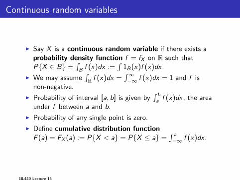
Continuous random variables
I Say X is a continuous random variable if there exists aprobability density function f = fX on R such thatP{X ∈ B} =
∫B f (x)dx :=
∫1B(x)f (x)dx .
I We may assume∫R f (x)dx =
∫∞−∞ f (x)dx = 1 and f is
non-negative.
I Probability of interval [a, b] is given by∫ ba f (x)dx , the area
under f between a and b.
I Probability of any single point is zero.
I Define cumulative distribution functionF (a) = FX (a) := P{X < a} = P{X ≤ a} =
∫ a−∞ f (x)dx .
18.440 Lecture 15

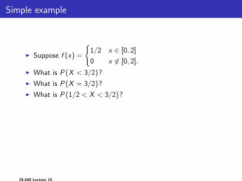
Simple example
I Suppose f (x) =
{1/2 x ∈ [0, 2]
0 x 6∈ [0, 2].
I What is P{X < 3/2}?I What is P{X = 3/2}?I What is P{1/2 < X < 3/2}?I What is P{X ∈ (0, 1) ∪ (3/2, 5)}?I What is F ?
I We say that X is uniformly distributed on the interval[0, 2].
18.440 Lecture 15

Simple example
I Suppose f (x) =
{1/2 x ∈ [0, 2]
0 x 6∈ [0, 2].
I What is P{X < 3/2}?
I What is P{X = 3/2}?I What is P{1/2 < X < 3/2}?I What is P{X ∈ (0, 1) ∪ (3/2, 5)}?I What is F ?
I We say that X is uniformly distributed on the interval[0, 2].
18.440 Lecture 15

Simple example
I Suppose f (x) =
{1/2 x ∈ [0, 2]
0 x 6∈ [0, 2].
I What is P{X < 3/2}?I What is P{X = 3/2}?
I What is P{1/2 < X < 3/2}?I What is P{X ∈ (0, 1) ∪ (3/2, 5)}?I What is F ?
I We say that X is uniformly distributed on the interval[0, 2].
18.440 Lecture 15
Simple example
I Suppose f (x) =
{1/2 x ∈ [0, 2]
0 x 6∈ [0, 2].
I What is P{X < 3/2}?I What is P{X = 3/2}?I What is P{1/2 < X < 3/2}?
I What is P{X ∈ (0, 1) ∪ (3/2, 5)}?I What is F ?
I We say that X is uniformly distributed on the interval[0, 2].
18.440 Lecture 15

Simple example
I Suppose f (x) =
{1/2 x ∈ [0, 2]
0 x 6∈ [0, 2].
I What is P{X < 3/2}?I What is P{X = 3/2}?I What is P{1/2 < X < 3/2}?I What is P{X ∈ (0, 1) ∪ (3/2, 5)}?
I What is F ?
I We say that X is uniformly distributed on the interval[0, 2].
18.440 Lecture 15

Simple example
I Suppose f (x) =
{1/2 x ∈ [0, 2]
0 x 6∈ [0, 2].
I What is P{X < 3/2}?I What is P{X = 3/2}?I What is P{1/2 < X < 3/2}?I What is P{X ∈ (0, 1) ∪ (3/2, 5)}?I What is F ?
I We say that X is uniformly distributed on the interval[0, 2].
18.440 Lecture 15

Simple example
I Suppose f (x) =
{1/2 x ∈ [0, 2]
0 x 6∈ [0, 2].
I What is P{X < 3/2}?I What is P{X = 3/2}?I What is P{1/2 < X < 3/2}?I What is P{X ∈ (0, 1) ∪ (3/2, 5)}?I What is F ?
I We say that X is uniformly distributed on the interval[0, 2].
18.440 Lecture 15

Another example
I Suppose f (x) =
{x/2 x ∈ [0, 2]
0 0 6∈ [0, 2].
I What is P{X < 3/2}?I What is P{X = 3/2}?I What is P{1/2 < X < 3/2}?I What is F ?
18.440 Lecture 15

Another example
I Suppose f (x) =
{x/2 x ∈ [0, 2]
0 0 6∈ [0, 2].
I What is P{X < 3/2}?
I What is P{X = 3/2}?I What is P{1/2 < X < 3/2}?I What is F ?
18.440 Lecture 15

Another example
I Suppose f (x) =
{x/2 x ∈ [0, 2]
0 0 6∈ [0, 2].
I What is P{X < 3/2}?I What is P{X = 3/2}?
I What is P{1/2 < X < 3/2}?I What is F ?
18.440 Lecture 15

Another example
I Suppose f (x) =
{x/2 x ∈ [0, 2]
0 0 6∈ [0, 2].
I What is P{X < 3/2}?I What is P{X = 3/2}?I What is P{1/2 < X < 3/2}?
I What is F ?
18.440 Lecture 15

Another example
I Suppose f (x) =
{x/2 x ∈ [0, 2]
0 0 6∈ [0, 2].
I What is P{X < 3/2}?I What is P{X = 3/2}?I What is P{1/2 < X < 3/2}?I What is F ?
18.440 Lecture 15

Outline
Continuous random variables
Expectation and variance of continuous random variables
Measurable sets and a famous paradox
18.440 Lecture 15

Outline
Continuous random variables
Expectation and variance of continuous random variables
Measurable sets and a famous paradox
18.440 Lecture 15
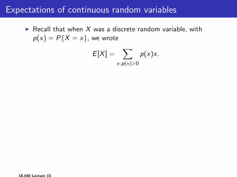
Expectations of continuous random variables
I Recall that when X was a discrete random variable, withp(x) = P{X = x}, we wrote
E [X ] =∑
x :p(x)>0
p(x)x .
I How should we define E [X ] when X is a continuous randomvariable?
I Answer: E [X ] =∫∞−∞ f (x)xdx .
I Recall that when X was a discrete random variable, withp(x) = P{X = x}, we wrote
E [g(X )] =∑
x :p(x)>0
p(x)g(x).
I What is the analog when X is a continuous random variable?
I Answer: we will write E [g(X )] =∫∞−∞ f (x)g(x)dx .
18.440 Lecture 15

Variance of continuous random variables
I Suppose X is a continuous random variable with mean µ.
I We can write Var[X ] = E [(X − µ)2], same as in the discretecase.
I Next, if g = g1 + g2 thenE [g(X )] =
∫g1(x)f (x)dx +
∫g2(x)f (x)dx =∫ (
g1(x) + g2(x))f (x)dx = E [g1(X )] + E [g2(X )].
I Furthermore, E [ag(X )] = aE [g(X )] when a is a constant.
I Just as in the discrete case, we can expand the varianceexpression as Var[X ] = E [X 2 − 2µX + µ2] and use additivityof expectation to say thatVar[X ] = E [X 2]− 2µE [X ] + E [µ2] = E [X 2]− 2µ2 + µ2 =E [X 2]− E [X ]2.
I This formula is often useful for calculations.
18.440 Lecture 15

Examples
I Suppose that fX (x) =
{1/2 x ∈ [0, 2]
0 x 6∈ [0, 2]..
I What is Var[X ]?
I Suppose instead that fX (x) =
{x/2 x ∈ [0, 2]
0 0 6∈ [0, 2].
I What is Var[X ]?
18.440 Lecture 15

Examples
I Suppose that fX (x) =
{1/2 x ∈ [0, 2]
0 x 6∈ [0, 2]..
I What is Var[X ]?
I Suppose instead that fX (x) =
{x/2 x ∈ [0, 2]
0 0 6∈ [0, 2].
I What is Var[X ]?
18.440 Lecture 15

Examples
I Suppose that fX (x) =
{1/2 x ∈ [0, 2]
0 x 6∈ [0, 2]..
I What is Var[X ]?
I Suppose instead that fX (x) =
{x/2 x ∈ [0, 2]
0 0 6∈ [0, 2].
I What is Var[X ]?
18.440 Lecture 15

Examples
I Suppose that fX (x) =
{1/2 x ∈ [0, 2]
0 x 6∈ [0, 2]..
I What is Var[X ]?
I Suppose instead that fX (x) =
{x/2 x ∈ [0, 2]
0 0 6∈ [0, 2].
I What is Var[X ]?
18.440 Lecture 15

Outline
Continuous random variables
Expectation and variance of continuous random variables
Measurable sets and a famous paradox
18.440 Lecture 15

Outline
Continuous random variables
Expectation and variance of continuous random variables
Measurable sets and a famous paradox
18.440 Lecture 15

Uniform measure on [0, 1]
I One of the very simplest probability density functions is
f (x) =
{1 x ∈ [0, 1]
0 0 6∈ [0, 1]..
I If B ⊂ [0, 1] is an interval, then P{X ∈ B} is the length ofthat interval.
I Generally, if B ⊂ [0, 1] then P{X ∈ B} =∫B 1dx =
∫1B(x)dx
is the “total volume” or “total length” of the set B.
I What if B is the set of all rational numbers?
I How do we mathematically define the volume of an arbitraryset B?
18.440 Lecture 15

Do all sets have probabilities? A famous paradox:
I Uniform probability measure on [0, 1) should satisfytranslation invariance: If B and a horizontal translation of Bare both subsets [0, 1), their probabilities should be equal.
I Consider wrap-around translations τr (x) = (x + r) mod 1.
I By translation invariance, τr (B) has same probability as B.
I Call x , y “equivalent modulo rationals” if x − y is rational(e.g., x = π − 3 and y = π − 9/4). An equivalence class isthe set of points in [0, 1) equivalent to some given point.
I There are uncountably many of these classes.
I Let A ⊂ [0, 1) contain one point from each class. For eachx ∈ [0, 1), there is one a ∈ A such that r = x − a is rational.
I Then each x in [0, 1) lies in τr (A) for one rational r ∈ [0, 1).
I Thus [0, 1) = ∪τr (A) as r ranges over rationals in [0, 1).
I If P(A) = 0, then P(S) =∑
r P(τr (A)) = 0. If P(A) > 0 thenP(S) =
∑r P(τr (A)) =∞. Contradicts P(S) = 1 axiom.
18.440 Lecture 15

Three ways to get around this
I 1. Re-examine axioms of mathematics: the very existenceof a set A with one element from each equivalence class isconsequence of so-called axiom of choice. Removing thataxiom makes paradox goes away, since one can just suppose(pretend?) these kinds of sets don’t exist.
I 2. Re-examine axioms of probability: Replace countableadditivity with finite additivity? (Look up Banach-Tarski.)
I 3. Keep the axiom of choice and countable additivity butdon’t define probabilities of all sets: Instead of definingP(B) for every subset B of sample space, restrict attention toa family of so-called “measurable” sets.
I Most mainstream probability and analysis takes the thirdapproach.
I In practice, sets we care about (e.g., countable unions ofpoints and intervals) tend to be measurable.
18.440 Lecture 15

Perspective
I More advanced courses in probability and analysis (such as18.125 and 18.175) spend a significant amount of timerigorously constructing a class of so-called measurable setsand the so-called Lebesgue measure, which assigns a realnumber (a measure) to each of these sets.
I These courses also replace the Riemann integral with theso-called Lebesgue integral.
I We will not treat these topics any further in this course.
I We usually limit our attention to probability density functionsf and sets B for which the ordinary Riemann integral∫
1B(x)f (x)dx is well defined.
I Riemann integration is a mathematically rigorous theory. It’sjust not as robust as Lebesgue integration.
18.440 Lecture 15
Related Documents