18–1. 18–2 Chapter Eighteen Copyright © 2014 by The McGraw-Hill Companies, Inc. All rights reserved. McGraw-Hill/Irwin.

18–1

Operations andSupply Chain Management

CHASE | SHANKAR | JACOBS

14e

18–2

FORECASTING

Chapter EighteenCopyright © 2014 by The McGraw-Hill Companies, Inc. All rights reserved.McGraw-Hill/Irwin

18–3

Cop

yri

gh

t ©

20

14

by M

cGra

w H

ill E

du

cati

on

(In

dia

) Pri

vate

Lim

ited

. A

ll ri

gh

ts

rese

rved

.

Learning Objectives

• LO18–1: Understand how forecasting is essential to supply chain planning

• LO18–2: Evaluate demand using quantitative forecasting models

• LO18–3: Apply qualitative techniques to forecast demand

• LO18–4: Apply collaborative techniques to forecast demand

18–4

Cop

yri

gh

t ©

20

14

by M

cGra

w H

ill E

du

cati

on

(In

dia

) Pri

vate

Lim

ited

. A

ll ri

gh

ts

rese

rved

.The Role of Forecasting

• Forecasting is a vital function and affects every significant management decision.– Finance and accounting use forecasts as the basis for

budgeting and cost control.

– Marketing relies on forecasts to make key decisions such as new product planning and personnel compensation.

– Production uses forecasts to select suppliers; determine capacity requirements; and drive decisions about purchasing, staffing, and inventory.

• Different roles require different forecasting approaches.– Decisions about overall directions require strategic forecasts.

– Tactical forecasts are used to guide day-to-day decisions.

18–5

Cop

yri

gh

t ©

20

14

by M

cGra

w H

ill E

du

cati

on

(In

dia

) Pri

vate

Lim

ited

. A

ll ri

gh

ts

rese

rved

.Forecasting and Decoupling Point

• Decoupling point: Point at which inventory is stored, which allows SC to operate independently.

• The choice of the decoupling point in a SC is strategic.

• Forecasting helps determine the level of inventory needed at the decoupling points.

• The decision will be affected by the error produced in the forecast and the type of product (easily inventoried or easily perishable).

18–6

Cop

yri

gh

t ©

20

14

by M

cGra

w H

ill E

du

cati

on

(In

dia

) Pri

vate

Lim

ited

. A

ll ri

gh

ts

rese

rved

.

Types of Forecasting

• There are four basic types of forecasts.– Qualitative– Time series analysis (primary focus of this

chapter)– Causal relationships– Simulation

• Time series analysis is based on the idea that data relating to past demand can be used to predict future demand.

18–7

Cop

yri

gh

t ©

20

14

by M

cGra

w H

ill E

du

cati

on

(In

dia

) Pri

vate

Lim

ited

. A

ll ri

gh

ts

rese

rved

.Components of Demand

Average demand for a period of time

Trend

Seasonal element

Cyclical elements

Random variation

Autocorrelation

Excel: Components of Demand

For the Excel template visit www.mhhe.com/sie-chase14e

18–8

Cop

yri

gh

t ©

20

14

by M

cGra

w H

ill E

du

cati

on

(In

dia

) Pri

vate

Lim

ited

. A

ll ri

gh

ts

rese

rved

.

Trends

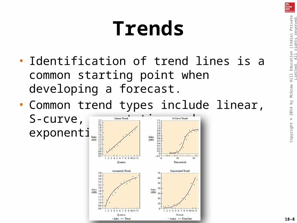
• Identification of trend lines is a common starting point when developing a forecast.

• Common trend types include linear, S-curve, asymptotic, and exponential.

18–9

Cop

yri

gh

t ©

20

14

by M

cGra

w H

ill E

du

cati

on

(In

dia

) Pri

vate

Lim

ited

. A

ll ri

gh

ts

rese

rved

.

Time Series Analysis

• Using the past to predict the future

• Used mainly for tactical decisions

Short term – forecasting less than 3 months

• Used to develop a strategy that will be implemented over the next 6 to 18 months (e.g., meeting demand)

Medium term – forecasting 3 months to 2 years

• Useful for detecting general trends and identifying major turning points

Long term – forecasting greater than 2 years

18–10

Cop

yri

gh

t ©

20

14

by M

cGra

w H

ill E

du

cati

on

(In

dia

) Pri

vate

Lim

ited

. A

ll ri

gh

ts

rese

rved

.

Model Selection

• Choosing an appropriate forecasting model depends upon– Time horizon to be forecast– Data availability– Accuracy required– Size of forecasting budget– Availability of qualified personnel

18–11

Cop

yri

gh

t ©

20

14

by M

cGra

w H

ill E

du

cati

on

(In

dia

) Pri

vate

Lim

ited

. A

ll ri

gh

ts

rese

rved

.

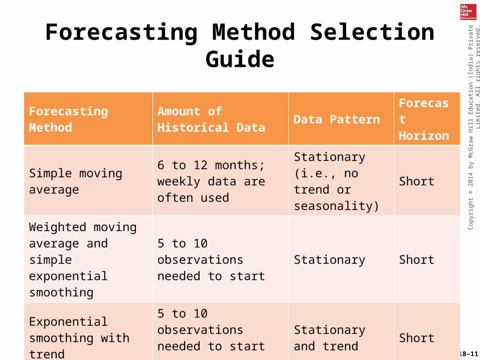
Forecasting Method Selection Guide

Forecasting Method

Amount of Historical Data Data Pattern

Forecast Horizon

Simple moving average

6 to 12 months; weekly data are often used

Stationary (i.e., no trend or seasonality)

Short

Weighted moving average and simple exponential smoothing

5 to 10 observations needed to start Stationary Short

Exponential smoothing with trend

5 to 10 observations needed to start Stationary and

trend Short

Linear regression 10 to 20 observations

Stationary, trend, and seasonality

Short to medium

18–12

Cop

yri

gh

t ©

20

14

by M

cGra

w H

ill E

du

cati

on

(In

dia

) Pri

vate

Lim

ited

. A

ll ri

gh

ts

rese

rved

.Simple Moving Average

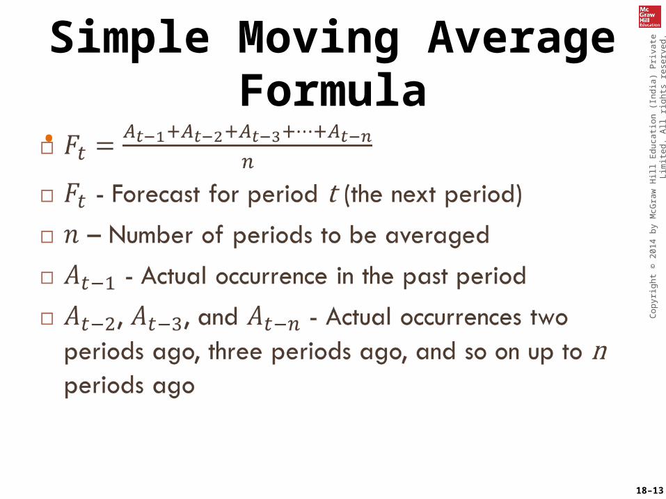
• Forecast is the average of a fixed number of past periods.

• Useful when demand is not growing or declining rapidly and no seasonality is present.

• Removes some of the random fluctuation from the data.

• Selecting the period length is important.– Longer periods provide more smoothing.

– Shorter periods react to trends more quickly.

18–13

Cop

yri

gh

t ©

20

14

by M

cGra

w H

ill E

du

cati

on

(In

dia

) Pri

vate

Lim

ited

. A

ll ri

gh

ts

rese

rved

.Simple Moving Average Formula

•  

18–14

Cop

yri

gh

t ©

20

14

by M

cGra

w H

ill E

du

cati

on

(In

dia

) Pri

vate

Lim

ited

. A

ll ri

gh

ts

rese

rved

.Simple Moving Average – Example

18-14

18–15

Cop

yri

gh

t ©

20

14

by M

cGra

w H

ill E

du

cati

on

(In

dia

) Pri

vate

Lim

ited

. A

ll ri

gh

ts

rese

rved

.Weighted Moving Average

• The simple moving average formula implies equal weighting for all periods.

• A weighted moving average allows unequal weighting of prior time periods.– The sum of the weights must be equal to one.

– Often, more recent periods are given higher weights than periods farther in the past.

𝐹 𝑡=𝑤1 𝐴𝑡−1+𝑤2 𝐴𝑡−2+…+𝑤𝑛𝐴𝑡−𝑛

18–16

Cop

yri

gh

t ©

20

14

by M

cGra

w H

ill E

du

cati

on

(In

dia

) Pri

vate

Lim

ited

. A

ll ri

gh

ts

rese

rved

.

Selecting Weights

• Experience and/or trial-and-error are the simplest approaches.

• The recent past is often the best indicator of the future, so weights are generally higher for more recent data.

• If the data are seasonal, weights should reflect this appropriately.

18–17

Cop

yri

gh

t ©

20

14

by M

cGra

w H

ill E

du

cati

on

(In

dia

) Pri

vate

Lim

ited

. A

ll ri

gh

ts

rese

rved

.Exponential Smoothing

• A weighted average method that includes all past data in the forecasting calculation

• More recent results weighted more heavily

• The most used of all forecasting techniques

• An integral part of computerized forecasting

18–18

Cop

yri

gh

t ©

20

14

by M

cGra

w H

ill E

du

cati

on

(In

dia

) Pri

vate

Lim

ited

. A

ll ri

gh

ts

rese

rved

.Exponential Smoothing

• Well accepted for six reasons– Exponential models are surprisingly accurate– Formulating an exponential model is

relatively easy– The user can understand how the model

works– Little computation is required to use the

model– Computer storage requirements are small– Tests for accuracy are easy to compute

18–19

Cop

yri

gh

t ©

20

14

by M

cGra

w H

ill E

du

cati

on

(In

dia

) Pri

vate

Lim

ited

. A

ll ri

gh

ts

rese

rved

.Exponential Smoothing Model

18-19

18–20

Cop

yri

gh

t ©

20

14

by M

cGra

w H

ill E

du

cati

on

(In

dia

) Pri

vate

Lim

ited

. A

ll ri

gh

ts

rese

rved

.Exponential Smoothing Example

18-20

Week Demand Forecast

1 820 820

2 775 820

3 680 811

4 655 785

5 750 759

6 802 757

7 798 766

8 689 772

9 775 756

10 760

18–21

Cop

yri

gh

t ©

20

14

by M

cGra

w H

ill E

du

cati

on

(In

dia

) Pri

vate

Lim

ited

. A

ll ri

gh

ts

rese

rved

.Exponential Smoothing – Effect of Trends

• The presence of a trend in the data causes the exponential smoothing forecast to always lag behind the actual data

• This can be corrected by adding a trend adjustment

– The trend smoothing constant is delta (δ)

18–22

Cop

yri

gh

t ©

20

14

by M

cGra

w H

ill E

du

cati

on

(In

dia

) Pri

vate

Lim

ited

. A

ll ri

gh

ts

rese

rved

.

Example – Exponential Smoothing with Trend Adjustment

• Calculate the new forecast, assuming the following:– The previous forecast including trend (FITt-1) is 110

and the previous estimate of the trend (Tt-1) is 10

– α = 0.2 and δ = 0.3– Actual demand for period t-1 is 115

Ft = Ft-1 + α(At-1 – FITt-1) = 110 + 0.2(115-110) = 111.0

Tt = Tt-1 + δ(Ft-1 – FITt-1) = 10 + 0.3(111-110) = 10.3

FITt = Ft + Tt = 111.0 + 10.3 = 121.3

18–23

Cop

yri

gh

t ©

20

14

by M

cGra

w H

ill E

du

cati

on

(In

dia

) Pri

vate

Lim

ited

. A

ll ri

gh

ts

rese

rved

.Choosing Alpha and Delta

• Relatively small values for α and δ are common– Usually in the range 0.1 to 0.3

• α depends upon how much random variation is present

• δ depends upon how steady the trend is

• Measurement of forecast error can be used to select values of α and δ to minimize overall forecast error

18–24

Cop

yri

gh

t ©

20

14

by M

cGra

w H

ill E

du

cati

on

(In

dia

) Pri

vate

Lim

ited

. A

ll ri

gh

ts

rese

rved

.Linear Regression Analysis

• Regression is used to identify the functional relationship between two or more correlated variables, usually from observed data.

• One variable (the dependent variable) is predicted for given values of the other variable (the independent variable).

• Linear regression is a special case that assumes the relationship between the variables can be explained with a straight line.

Y = a + bt 

18–25

Cop

yri

gh

t ©

20

14

by M

cGra

w H

ill E

du

cati

on

(In

dia

) Pri

vate

Lim

ited

. A

ll ri

gh

ts

rese

rved

.

Example 18.2 – Least Squares Method

• The least squares method determines the parameters a and b such that the sum of the squared errors is minimized – “least squares”

Quarter

Sales

Quarter

Sales

1 600 7 2,600

2 1,550 8 2,90

0

3 1,500 9 3,80

0

4 1,500 10 4,50

0

5 2,400 11 4,00

0

6 3,100 12 4,90

0

18–26

Cop

yri

gh

t ©

20

14

by M

cGra

w H

ill E

du

cati

on

(In

dia

) Pri

vate

Lim

ited

. A

ll ri

gh

ts

rese

rved

.Example 18.2 – Calculations

1 600 600 1 360,000 801.3

2 1,550 3,100 4 2,402,500 1,160.9

3 1,500 4,500 9 2,250,000 1,520.5

4 1,500 6,000 16 2,250,000 1,880.1

5 2,400 12,000 25 5,760,000 2,239.7

6 3,100 18,600 36 9,610,000 2,599.4

7 2,600 18,200 49 6,760,000 2,959.0

8 2,900 23,200 64 8,410,000 3,318.6

9 3,800 34,200 81 14,440,000 3,678.2

10 4,500 45,000 100 20,250,000 4,037.8

11 4,000 44,000 121 16,000,000 4,397.4

12 4,900 58,800 144 24,010,000 4,757.1

Sum   78   33,350    268,200   650    112,502,500 

18-26

 The forecast is extended to periods 13-16

18–27

Cop

yri

gh

t ©

20

14

by M

cGra

w H

ill E

du

cati

on

(In

dia

) Pri

vate

Lim

ited

. A

ll ri

gh

ts

rese

rved

.

Regression with Excel

• Microsoft Excel includes data analysis tools, which can perform least squares regression on a data set.

18–28

Cop

yri

gh

t ©

20

14

by M

cGra

w H

ill E

du

cati

on

(In

dia

) Pri

vate

Lim

ited

. A

ll ri

gh

ts

rese

rved

.Time Series Decomposition

• Chronologically ordered data are referred to as a time series.

• A time series may contain one or many elements.– Trend, seasonal, cyclical, autocorrelation,

and random

• Identifying these elements and separating the time series data into these components is known as decomposition.

18–29

Cop

yri

gh

t ©

20

14

by M

cGra

w H

ill E

du

cati

on

(In

dia

) Pri

vate

Lim

ited

. A

ll ri

gh

ts

rese

rved

.

Seasonal Variation

• Seasonal variation may be either additive or multiplicative (shown here with a changing trend).

18–30

Cop

yri

gh

t ©

20

14

by M

cGra

w H

ill E

du

cati

on

(In

dia

) Pri

vate

Lim

ited

. A

ll ri

gh

ts

rese

rved

.

Season Past SalesAverage Sales for Each Season

Seasonal Factor

Spring 200 = 250 = 0.8Summer 350 = 250 = 1.4Fall 300 = 250 = 1.2Winter 150 = 250 = 0.6Total 1000

Determining Seasonal Factors : Simple Proportions Example 18.3

• The seasonal factor (or index) is the ratio of the amount sold during each season divided by the average for all seasons.

18–31

Cop

yri

gh

t ©

20

14

by M

cGra

w H

ill E

du

cati

on

(In

dia

) Pri

vate

Lim

ited

. A

ll ri

gh

ts

rese

rved

.

Example 18.3 (Continued)

ExpectedDemand forNext Year

AverageSales forEach Season(1,100y4)

SeasonalFactor

Next Year’sSeasonalForecast

Spring 275 X 0.8 = 220

Summer 275 X 1.4 = 385

Fall 275 X 1.2 = 330

Winter 275 X 0.6 = 165

1100

18–32

Cop

yri

gh

t ©

20

14

by M

cGra

w H

ill E

du

cati

on

(In

dia

) Pri

vate

Lim

ited

. A

ll ri

gh

ts

rese

rved

.Decomposition Using Least Squares Regression

• Decompose the time series into its components– Find seasonal component

– Deseasonalize the demand

– Find trend component

• Forecast future values of each component– Project trend component into the future

– Multiply trend component by seasonal component

18–33

Cop

yri

gh

t ©

20

14

by M

cGra

w H

ill E

du

cati

on

(In

dia

) Pri

vate

Lim

ited

. A

ll ri

gh

ts

rese

rved

.Decomposition – Steps 1 and 2

• Using the data for periods 1-12, apply time series analysis (decomposition, linear regression, trend estimate & seasonal indices) to forecast for periods 13-16

18–34

Cop

yri

gh

t ©

20

14

by M

cGra

w H

ill E

du

cati

on

(In

dia

) Pri

vate

Lim

ited

. A

ll ri

gh

ts

rese

rved

.Decomposition – Steps 3 and 4

• Develop a least squares regression line for the deseasonalized data.

• Project the regression line through the period of the forecast.

Regression Results: Y = 555.0 + 342.2t

Forecast for periods 13-16

18–35

Cop

yri

gh

t ©

20

14

by M

cGra

w H

ill E

du

cati

on

(In

dia

) Pri

vate

Lim

ited

. A

ll ri

gh

ts

rese

rved

.

Decompostion – Step 5

• Create the final forecast by adjusting the regression line by the seasonal factor.

Period

Quarter

Y from Regression

Seasonal Factor

Forecast (F x Seasonal Factor

13 I 5,003.5 0.82 4,102.87

14 II 5,345.7 1.10 5,880.27

15 III 5,687.9 0.97 5,517.26

16 IV 6,030.1 1.12 6,753.71

18–36

Cop

yri

gh

t ©

20

14

by M

cGra

w H

ill E

du

cati

on

(In

dia

) Pri

vate

Lim

ited

. A

ll ri

gh

ts

rese

rved

.

Forecast Errors

• Forecast error is the difference between the forecast value and what actually occurred.

• All forecasts contain some level of error.

• Sources of error– Bias – when a consistent mistake is made

– Random – errors that are not explained by the model being used

• Measures of error– Mean absolute deviation (MAD)

– Mean absolute percent error (MAPE)

– Tracking signal

18–37

Cop

yri

gh

t ©

20

14

by M

cGra

w H

ill E

du

cati

on

(In

dia

) Pri

vate

Lim

ited

. A

ll ri

gh

ts

rese

rved

.Forecast Error Measurements

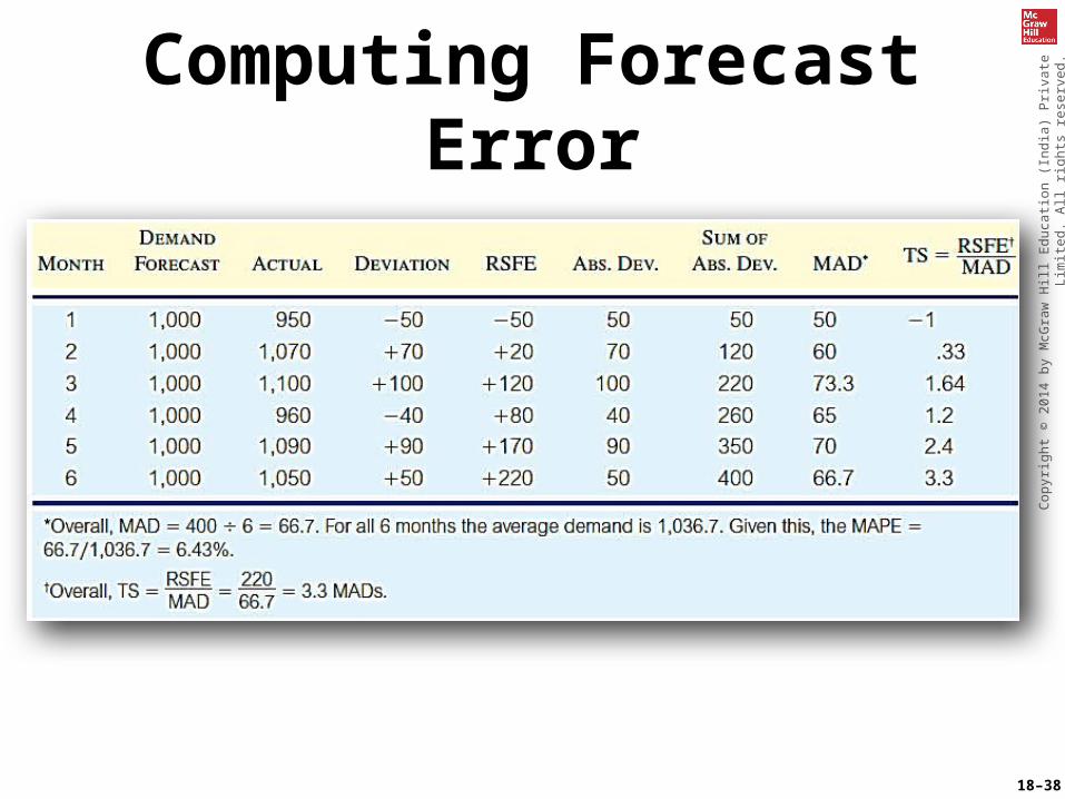
• Ideally, MAD will be zero (no forecasting error).

• Larger values of MAD indicate a less accurate model.

• MAPE scales the forecast error to the magnitude of demand.

• Tracking signal indicates whether forecast errors are accumulating over time (either positive or negative errors).

18–38

Cop

yri

gh

t ©

20

14

by M

cGra

w H

ill E

du

cati

on

(In

dia

) Pri

vate

Lim

ited

. A

ll ri

gh

ts

rese

rved

.Computing Forecast Error

18–39

Cop

yri

gh

t ©

20

14

by M

cGra

w H

ill E

du

cati

on

(In

dia

) Pri

vate

Lim

ited

. A

ll ri

gh

ts

rese

rved

.Causal Relationship Forecasting

• Causal relationship forecasting uses independent variables other than time to predict future demand.– This independent variable must be a leading

indicator.

• Many apparently causal relationships are actually just correlated events – care must be taken when selecting causal variables.

18–40

Cop

yri

gh

t ©

20

14

by M

cGra

w H

ill E

du

cati

on

(In

dia

) Pri

vate

Lim

ited

. A

ll ri

gh

ts

rese

rved

.Multiple Regression Techniques

• Often, more than one independent variable may be a valid predictor of future demand.

• In this case, the forecast analyst may utilize multiple regression.– Analogous to linear regression analysis,

but with multiple independent variables.–Multiple regression supported by

statistical software packages.

18–41

Cop

yri

gh

t ©

20

14

by M

cGra

w H

ill E

du

cati

on

(In

dia

) Pri

vate

Lim

ited

. A

ll ri

gh

ts

rese

rved

.

Qualitative Forecasting Techniques

• Generally used to take advantage of expert knowledge.

• Useful when judgment is required, when products are new, or if the firm has little experience in a new market.

• Examples– Market research

– Panel consensus

– Historical analogy

– Delphi method

18–42

Cop

yri

gh

t ©

20

14

by M

cGra

w H

ill E

du

cati

on

(In

dia

) Pri

vate

Lim

ited

. A

ll ri

gh

ts

rese

rved

.

Collaborative Planning, Forecasting, and Replenishment (CPFR)

• A web-based process used to coordinate the efforts of a supply chain.– Demand forecasting

– Production and purchasing

– Inventory replenishment

• Integrates all members of a supply chain – manufacturers, distributors, and retailers.

• Depends upon the exchange of internal information to provide a more reliable view of demand.

18–43

Cop

yri

gh

t ©

20

14

by M

cGra

w H

ill E

du

cati

on

(In

dia

) Pri

vate

Lim

ited

. A

ll ri

gh

ts

rese

rved

.

CPFR Steps

Creation of a front-end

partnership agreement

Joint business planning

Development of demand forecasts

Sharing forecasts

Inventory replenishmen

t

18–44

Cop

yri

gh

t ©

20

14

by M

cGra

w H

ill E

du

cati

on

(In

dia

) Pri

vate

Lim

ited

. A

ll ri

gh

ts

rese

rved

.

Principles• Forecasting is a fundamental step in any planning

process.

• Forecast effort should be proportional to the magnitude of decisions being made.

• Web-based systems (CPFR) are growing in importance and effectiveness.

• All forecasts have errors – understanding and minimizing this error is the key to effective forecasting processes.