18.06 Problem Set 5 - Solutions18.06 Problem Set 5 - Solutions Due Wednesday, 17 October 2007 at 4 pm in 2-106. Problem 1: (10) Do problem 22 from section 4.1 (P 193) in your book.

18.06 Problem Set 5 - SolutionsDue Wednesday, 17 October 2007 at 4 pm in 2-106.

Problem 1: (10) Do problem 22 from section 4.1 (P 193) in your book.

Solution The equation x1 + x2 + x3 + x4 = 0 can be rewritten in the matrix form

(1 1 1 1

) x1

x2

x3

x4

= 0.

Thus P is the nullspace of the 1 by 4 matrix

A =(1 1 1 1

).

This implies that P⊥ is the row space of A. Obviously a basis of P⊥ is given by thevector

v =

1111

.

Problem 2: (15=6+3+6) (1) Derive the Fredholm Alternative: If the system Ax =b has no solution, then argue there is a vector y satisfying

ATy = 0 with yTb = 1.

(Hint: b is not in the column space C(A), thus b is not orthogonal to N(AT ).)

Solution Suppose the system Ax = b has no solution, in other words, the vectorb does not lie in the column space C(A). Then b is not orthogonal to the nullspaceN(AT ). Let p be the orthogonal projection of b onto N(AT ), then p 6= 0. We have

pTb = pTp 6= 0.

Let y = 1pT p

p, we see that

ATy =1

pTpATp = 0

1

but

yTb =1

pTppTb = 1.

(2) Check that the following system Ax = b has no solution:

x + 2y + 2z = 2

2x + 2y + 3z = 1

3x + 2y + 4z = 2

Solution We do Gauss elimination:1 2 2 22 2 3 13 2 4 2

→

1 2 2 20 −2 −1 −30 −4 −2 −4

→

1 2 2 20 −2 −1 −30 0 0 2

,

which certainly has no solution.

(3) Find a vector y for above system such that ATy = 0 and yTb = 1.

Solution From solution to part (1) one need to find the projection of the vector bonto the N(AT ). We compute N(AT ):

A =

1 2 22 2 33 2 4

⇒ AT =

1 2 32 2 22 3 4

→

1 2 30 −2 −40 −1 −2

→

1 2 30 −2 −40 0 0

.

So the nullspace N(AT ) is spanned by one vector a =

1−21

.

The projection of b on the this line is

p =aTb

aTaa =

2− 2 + 2

1 + 4 + 1a =

2

6a =

1/3−2/31/3

So the vector y we need is

y =1

pTpp =

1

1/9 + 4/9 + 1/9p =

1/2−11/2

2

Problem 3: (10=2+2+2+2+2) Justify the following (true) statements:

(1) If AB = 0, then the column space of B is in the nullspace of A.

Solution If not, i.e., there is a vector y = Bx lies in the column space of B, butnot in the nullspace of A. Then

(AB)x = A(Bx) 6= 0,

contradicts with AB = 0.

(2) If A is symmetric matrix, then its column space is perpendicular to its nullspace.

Solution Since A is symmetric, A = AT . So its columm space coincides with itsrow space: C(A) = C(AT ). This implies that its column space is perpendicular toits nullspace.

(3) If a subspace S is contained in a subspace V , then S⊥ contains V ⊥.

Solution Suppose v ∈ V ⊥, i.e., v is perpendicular to any vector in V . In particular,v is perpendicular to any vector in S, since S ⊂ V . This shows that v ∈ S⊥. SoS⊥ ⊃ V ⊥.

(4) For any subspace V , (V ⊥)⊥ = V .

Solution By definition, V ⊥ is the set of vectors that are perpendicular to all vectorsin V . So any vector in V is perpendicular to all vectors in V ⊥. This impliesV ⊂ (V ⊥)⊥. On the other hand, suppose the dimension of V is r, then the dimensionof V ⊥ is n− r, and the dimension of (V ⊥)⊥ is again r. So a basis of V is also a basisof (V ⊥)⊥. This implies (V ⊥)⊥ = V .

(Another way: any subspace V is defined by some linear equations, in otherwords, V = N(A) is the nullspace for some matrix A. Thus V ⊥ = C(AT ) by thefundamental theorm of linear algebra. Use this theorem again we get (V ⊥)⊥ =N((AT )T ) = N(A) = V .)

(The proofs above only work for finite dimensional spaces. However, the state-ment is true for any closed subspaces in infinitely dimensional vector spaces, andthe proof is much harder.)

(5) If P is a projection matrix, so is I − P .

Solution Suppose P is the projection matrix onto a subspace V . Then I−P is theprojection matrix that projects onto V ⊥. In fact, for any vector v,

v − (I − P )v = v − v + Pv = Pv,

and obviously Pv ∈ V is perpendicular to V ⊥.

3

Problem 4: (10=5+5) (1) Do problem 5 from section 4.2 (P 203) in your book.

Solution We compute

P1 =a1a

T1

aT1 a1

=1

1 + 4 + 4

1 −2 −2−2 4 4−2 4 4

=1

9

1 −2 −2−2 4 4−2 4 4

,

P2 =a2a

T2

aT2 a2

=1

4 + 4 + 1

4 4 −24 4 −2−2 −2 1

=1

9

4 4 −24 4 −2−2 −2 1

.

Their product is

P1P2 =1

9

1 −2 −2−2 4 4−2 4 4

1

9

4 4 −24 4 −2−2 −2 1

=

0 0 00 0 00 0 0

.

This product is identically zero, since a1 and a2 are perpendicular, and thus ifwe first project a vector onto a1, then project the projection onto a2, we will get thezero vector.

(2) Do problem 7 from section 4.2 (P 203) in your book.

Solution The matrix P3 is

P3 =a3a

T3

aT3 a3

=1

4 + 1 + 4

4 −2 4−2 1 −24 −2 4

=1

9

4 −2 4−2 1 −24 −2 4

.

Obviously that

P1 + P2 + P3 =1

9

9 0 00 9 00 0 9

= I.

Finally we verify that a1, a2, a3 are orthogonal:

aT1 a2 = −2 + 4− 2 = 0;

aT1 a3 = −2− 2 + 4 = 0;

aT2 a3 = 4− 2− 2 = 0.

4

Problem 5: (15=5+5+5) (1) Find the projection matrix PC onto the column spaceof

A =

(1 2 14 8 4

).

Solution By observation it is easy to see that the column space of A is the one

dimensional subspace containing the vector a =

(14

). Thus the projection matrix

is

PC =aaT

aTa=

1

17

(1 44 16

).

(2) Find the projection matrix PR onto the row space of the above matrix.

Solution By observation the row space of the matrix A is the one dimensional

subspace containing the vector b =

121

. Thus the projection matrix is

PR =bbT

bTb=

1

6

1 2 12 4 21 2 1

.

(3) What is PCAPR? Explain your result.

Solution We calculate

PCAPR =1

17

(1 44 16

)·(

1 2 14 8 4

)· 1

6

1 2 12 4 21 2 1

=

1

6

(1 2 14 8 4

) 1 2 12 4 21 2 1

=

(1 2 14 8 4

)= A.

For any vector v, we see v − PRv is always perpendicular to the row space ofA, thus v − PRv ∈ N(A). So A(v − PRv) = 0, i.e. Av = APRv. This impliesA = APR. Similarly, Av ∈ C(A) implies PCAv = Av, i.e., A = PCA. So we alwayshave PCAPR = PC(APR) = PCA = A.

5

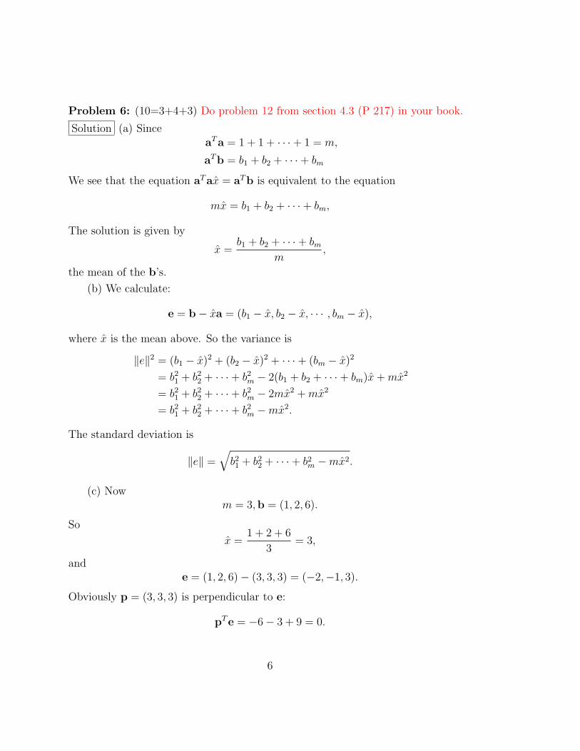
Problem 6: (10=3+4+3) Do problem 12 from section 4.3 (P 217) in your book.

Solution (a) SinceaTa = 1 + 1 + · · ·+ 1 = m,

aTb = b1 + b2 + · · ·+ bm

We see that the equation aTax̂ = aTb is equivalent to the equation

mx̂ = b1 + b2 + · · ·+ bm,

The solution is given by

x̂ =b1 + b2 + · · ·+ bm

m,

the mean of the b’s.

(b) We calculate:

e = b− x̂a = (b1 − x̂, b2 − x̂, · · · , bm − x̂),

where x̂ is the mean above. So the variance is

‖e‖2 = (b1 − x̂)2 + (b2 − x̂)2 + · · ·+ (bm − x̂)2

= b21 + b2

2 + · · ·+ b2m − 2(b1 + b2 + · · ·+ bm)x̂ + mx̂2

= b21 + b2

2 + · · ·+ b2m − 2mx̂2 + mx̂2

= b21 + b2

2 + · · ·+ b2m −mx̂2.

The standard deviation is

‖e‖ =√

b21 + b2

2 + · · ·+ b2m −mx̂2.

(c) Nowm = 3,b = (1, 2, 6).

So

x̂ =1 + 2 + 6

3= 3,

ande = (1, 2, 6)− (3, 3, 3) = (−2,−1, 3).

Obviously p = (3, 3, 3) is perpendicular to e:

pTe = −6− 3 + 9 = 0.

6

Problem 7: (10=5+5) In this problem you will derive weighted least-squares fits.In particular, suppose that you have m data points (ti, bi), that you want to fit toa line b = C + Dt. Ordinary least squares would choose C and D to minimize thesum-of-squares error

∑i(C + Dti − bi)

2, as derived in class. However, not all datapoints are always created equal: often, real data points come with a margin of errorσi > 0 in bi. When choosing C and D, we want to weight the data points less ifthey have more error. In particular, we want to choose C and D to minimize theerror ε given by:

ε =m∑

i=1

(C + Dti − bi

σi

)2

.

(a) Write ε in matrix form, just as for ordinary least squares in class (i.e. with amatrix A of 1s and ti values and a vector b of bi values), but using the additionaldiagonal “weighting” matrix W with Wii = 1/σi and Wij = 0 for i 6= j.

Solution In matrix formε = ‖WAx−Wb‖2,

where

A =

1 t11 t2...

...1 tm

, W =

1/σ1 0 · · · 0

0 1/σ2 · · · 0...

......

...0 0 · · · 1/σm.

(b) Derive a linear equation whose solution is the 2-component vector x (x1 = C,x2 = D) minimizing ε.

Solution Now we are minimizing

‖WAx−Wb‖2.

This is just the ordinary least square problem with A replaced by WA, and breplaced by Wb. So the linear equation whose solution minimizing ε is

(WA)T (WA)x̂ = (WA)T Wb,

i.e.AT W 2Ax̂ = AT W 2b.

More explicitly, (∑1/σ2

i

∑ti/σ

2i∑

ti/σ2i

∑t2i /σ

2i

) (CD

)=

( ∑bi/σ

2i∑

tibi/σ2i

).

7

Problem 8: (20=4+4+2+5+5) For this problem, you will generate some randomdata points from b = C + Dt + noise for C = 1 and D = 0.5, and then try to useleast-square fitting to recover C and D.

(a) First, generate m random data points for m = 20 and t ∈ (0, 10):

m = 20

t = rand(m,1) * 10

b = 1 + 0.5*t + (rand(m,1)-0.5)

The last line generates the data points from C + Dt plus random numbers in(−0.5, 0.5). Plot them with:

plot(t, b, ’o’)

Solution The codes

>> m=20;t=rand(m,1)*10,b=1+0.5*t+(rand(m,1)-0.5),plot(t,b,’o’)

t =

4.3874

3.8156

7.6552

7.9520

1.8687

4.8976

4.4559

6.4631

7.0936

7.5469

2.7603

6.7970

6.5510

1.6261

1.1900

4.9836

9.5974

3.4039

8

5.8527

2.2381

b =

3.4450

2.6629

4.8335

5.1751

2.3253

3.9081

3.2751

3.8702

4.1961

4.5309

2.7208

4.1528

4.5898

1.5566

2.0243

3.3418

5.4953

2.4530

4.0424

2.0923

9

1 2 3 4 5 6 7 8 9 101.5

2

2.5

3

3.5

4

4.5

5

5.5

Figure 1: t-b

(b) Now, do the least-square fit, as in class, by constructing the matrix A:

A = [ ones(m, 1), t ]

and then solving AT Ax̂ = ATb for x̂ = (C; D):

x = (A’ * A) \ (A’ * b)

(Refer to the 18.06 Matlab cheat-sheet if some of these commands confuse you.)Plot the least-square fit, along with the “real” line 1 + t/2:

t0 = [0; 10]

plot(t, b, ’bo’, t0, x(1) + t0*x(2), ’r-’, t0, 1 + t0/2, ’k--’)

(The data points should be blue circles, the least-square fit a red line, and the “real”line a black dashed line.)

Solution Codes

>> A=[ones(m,1),t];x=(A’*A)\(A’*b),t0=[0;10];

plot(t,b,’bo’,t0,x(1)+t0*x(2),’r-’,t0,1+t0/2,’k--’)

x =

1.2264

0.4565

10

0 1 2 3 4 5 6 7 8 9 101

1.5

2

2.5

3

3.5

4

4.5

5

5.5

6

Figure 2: least-square

(c) Verify that you get the same x by either of the two commands:

x = A \ b

x = pinv(A) * b

Solution Codes

>> x=A \ b

x =

1.2264

0.4565

>> x=pinv(A)*b

x =

1.2264

0.4565

11

(d) Repeat the least-square fit process above (you can skip the plots) for increasingnumbers of data points: m = 40, 80, 160, 320, 640, 1280 (and more, if you want). Foreach one, compute the squared error E in the least-square C and D compared totheir “real” values in the formula that the data is generated from:

E = (x(1) - 1)^2 + (x(2) - 0.5)^2

Plot this squared error versus m on a log-log scale using the command loglog inMatlab (which works just like plot but with logarithmic axes). Overall, you shouldfind that the error decreases with m: with more data points, the noise in the dataaverages out and the fit gets closer and closer to the underlying formula b = 1+ t/2.Note that if you want to create an array of E values, you can assign the elementsone by one via E(1) = ...; E(2) = ...; and so on. (Or you can write a loop, forVI-3 hackers.)

Solution Codes

>> m=40;t=rand(m,1)*10;b=1+0.5*t+(rand(m,1)-0.5);A=[ones(m,1),t];

x=(A’*A)\(A’*b);E(1)=(x(1)-1)^2+(x(2)-0.5)^2

E =

0.0073

>> m=80;t=rand(m,1)*10;b=1+0.5*t+(rand(m,1)-0.5);A=[ones(m,1),t];

x=(A’*A)\(A’*b);E(2)=(x(1)-1)^2+(x(2)-0.5)^2

E =

0.0073 0.0019

>> m=160;t=rand(m,1)*10;b=1+0.5*t+(rand(m,1)-0.5);A=[ones(m,1),t];

x=(A’*A)\(A’*b);E(3)=(x(1)-1)^2+(x(2)-0.5)^2

E =

0.0073 0.0019 0.0018

>> m=320;t=rand(m,1)*10;b=1+0.5*t+(rand(m,1)-0.5);A=[ones(m,1),t];

x=(A’*A)\(A’*b);E(4)=(x(1)-1)^2+(x(2)-0.5)^2

12

E =

0.0073 0.0019 0.0018 0.0008

>> m=640;t=rand(m,1)*10;b=1+0.5*t+(rand(m,1)-0.5);A=[ones(m,1),t];

x=(A’*A)\(A’*b);E(5)=(x(1)-1)^2+(x(2)-0.5)^2

E =

0.0073 0.0019 0.0018 0.0008 0.0004

>> m=1280;t=rand(m,1)*10;b=1+0.5*t+(rand(m,1)-0.5);A=[ones(m,1),t];

x=(A’*A)\(A’*b);E(6)=(x(1)-1)^2+(x(2)-0.5)^2

E =

0.0073 0.0019 0.0018 0.0008 0.0004 0.0001

>> m(1)=40;m(2)=80;m(3)=160;m(4)=320;m(5)=640;m(6)=1280;loglog(m,E,’bo’)

101

102

103

104

10−5

10−4

10−3

10−2

Figure 3: m-E

13

(e) Overall, E should depend on m as some power law: E = α ∗ mβ for someconstants α and β (plus random noise, of course). Find α and β by a least-squarefit of log E versus log m (since log E = log α+β log m is a straight line). (Show yourcode!)

Solution Codes

>> lm(1)=log(m(1));lm(2)=log(m(2));lm(3)=log(m(3));lm(4)=log(m(4));

lm(5)=log(m(5));lm(6)=log(m(6));

>> le(1)=log(E(1));le(2)=log(E(2));le(3)=log(E(3));le(4)=log(E(4));

le(5)=log(E(5));le(6)=log(E(6));

>> B=[ones(6,1),lm’];y=(B’*B)\(B’*le’)

y =

-0.8137

-1.1346

Thus α = e−0.8137 = 0.4432, β = −1.1346.

(More accurate solution should go to about α=0.12, β=-1. Prof. Johnson tried itfor 10000 random m values log-distributed from 10 to 10000 — see the graph below.The actual student answers will vary quite a bit because of random variations, ofcourse (for the suggested data set of only 6 data points, the standard deviation ofbeta seems to be about 0.7).)

14

101

102

103

104

10−10

10−9

10−8

10−7

10−6

10−5

10−4

10−3

10−2

10−1

100

number of data points (m)

erro

r E

in le

ast−

squa

re fi

t par

amet

ers

data points E

fit E = 0.12243 m−1.0072

Figure 4: m-E

15

For problem 3(iv), we would ideally like to prove (V ⊥)⊥ = V for “any” subspaceV without assuming a finite-dimensional vector space. We need to show both V ⊂(V ⊥)⊥ and (V ⊥)⊥ ⊂ V :

• If v ∈ V , then v is perpendicular to everything in V ⊥, by definition, so v ∈(V ⊥)⊥.

• If y ∈ (V ⊥)⊥, let v be the closest point1 in V to y, i.e. v is the point in Vthat minimizes ‖y − v‖2—we now must show that y = v. In class, we showedy − v ∈ V ⊥ for finite-dimensional spaces, using calculus; if we can show thesame thing in general we are done: y ∈ (V ⊥)⊥ implies that y = (y − v) + v isperpendicular to everything in V ⊥, which implies that y−v is perpendicular toeverything in V ⊥ (since v is perpendicular to V ⊥), which implies that y− v is0 (the only element of V ⊥ that is also perpendicular to V ⊥), and hence y = v.

• To show y − v ∈ V ⊥, consider any point v′ ∈ V and any real number λ(assuming our vector space is over the reals). V is a subspace, so v + λv′ ∈ V ,and v is the closest point in V to y, so ‖y−v‖2 ≤ ‖y−(v+λv′)‖2 = ‖y−v‖2 +λ2‖v′‖2−2λv′ ·(y−v). Choose the sign of λ so that λv′ ·(y−v) = |λv′ ·(y−v)|.Then, by simple algebra, |v′ · (y− v)| ≤ |λ|

2‖v′‖2, and if we let λ → 0 we obtain

v′ · (y − v) = 0. Q.E.D.

A good source for more information on this sort of thing is Basic Classes of LinearOperators by Gohberg, Goldberg, and Kaashoek (Birkhauser, 2003).

1This glosses over one tricky point: how do we know that there is a “closest” point to y in V ,i.e. that infv∈V ‖y − v‖2 is actually attained for some v? To have this, we must require that V bea closed subspace. In practice, unless you are very perverse, any subspace you are likely to workwith will be closed.

16