
17450844 Statistics in Plain English Second Edition
Oct 30, 2014
Welcome message from author
This document is posted to help you gain knowledge. Please leave a comment to let me know what you think about it! Share it to your friends and learn new things together.
Transcript

Statistics in Plain English
Second Edition

This page intentionally left blank
Statistics in Plain English
Second Edition
by
Timothy C. UrdanSanta Clara University
LEA LAWRENCE ERLBAUM ASSOCIATES, PUBLISHERS2005 Mahwah, New Jersey London
Senior Editor: Debra RiegertEditorial Assistant: Kerry BreenCover Design: Kathryn Houghtaling LaceyTextbook Production Manager: Paul SmolenskiText and Cover Printer: Victor Graphics
The final camera copy for this work was prepared by the author, and therefore the publishertakes no responsibility for consistency or correctness of typographical style. However, this ar-rangement helps to make publication of this kind of scholarship possible.
Copyright © 2005 by Lawrence Erlbaum Associates, Inc.
All rights reserved. No part of this book may be reproduced in any form, by photostat,microform, retrieval system, or any other means, without prior written permission of thepublisher.
Lawrence Erlbaum Associates, Inc., Publishers10 Industrial AvenueMahwah, New Jersey 07430www.erlbaum.com
Library of Congress Cataloging-in-Publication Data
Urdan, Timothy C.Statistics in plain English / Timothy C. Urdan.
p. cm.
Includes bibliographical references and index.
ISBN 0-8058-5241-7 (pbk.: alk. paper)1. Statistics—Textbooks. I. Title.QA276.12.U75 2005519.5—dc22 2004056393
CIPBooks published by Lawrence Erlbaum Associates are printed on acid-free paper, and theirbindings are chosen for strength and durability.
Printed in the United States of America10 9 8 7 6 5 4 3 2 1
Disclaimer: This eBook does not include the ancillary media that waspackaged with the original printed version of the book.

ForJeannine, Ella, and Nathaniel

This page intentionally left blank
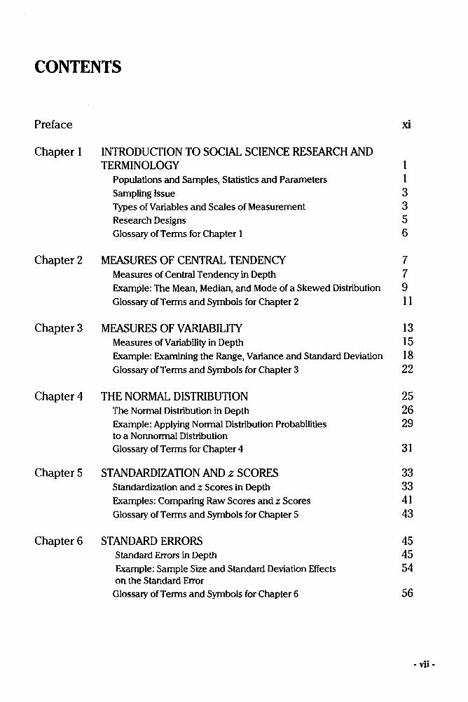
CONTENTS
Preface xi
Chapter 1 INTRODUCTION TO SOCIAL SCIENCE RESEARCH ANDTERMINOLOGY 1
Populations and Samples, Statistics and Parameters 1Sampling Issue 3Types of Variables and Scales of Measurement 3Research Designs 5Glossary of Terms for Chapter 1 6
Chapter 2 MEASURES OF CENTRAL TENDENCY 7Measures of Central Tendency in Depth 7Example: The Mean, Median, and Mode of a Skewed Distribution 9Glossary of Terms and Symbols for Chapter 2 11
Chapter 3 MEASURES OF VARIABILITY 13Measures of Variability in Depth 15Example: Examining the Range, Variance and Standard Deviation 18Glossary of Terms and Symbols for Chapter 3 22
Chapter 4 THE NORMAL DISTRIBUTION 25The Normal Distribution in Depth 26Example: Applying Normal Distribution Probabilities 29to a Nonnormal DistributionGlossary of Terms for Chapter 4 31
Chapter 5 STANDARDIZATION AND z SCORES 33Standardization and z Scores in Depth 33Examples: Comparing Raw Scores and z Scores 41Glossary of Terms and Symbols for Chapter 5 43
Chapter 6 STANDARD ERRORS 45Standard Errors in Depth 45Example: Sample Size and Standard Deviation Effects 54on the Standard ErrorGlossary of Terms and Symbols for Chapter 6 56
-vii-

- viii - CONTENTS
Chapter 7 STATISTICAL SIGNIFICANCE, EFFECT SIZE, 57AND CONFIDENCE INTERVALS
Statistical Significance in Depth 58Effect Size in Depth 63Confidence Intervals in Depths 66Example: Statistical Significance, Confidence Interval, 68and Effect Size for a One-Sample t Test of MotivationGlossary of Terms and Symbols for Chapter 7 72
Chapter 8 CORRELATION 75Pearson Correlation Coefficient in Depth 77A Brief Word on Other Types of Correlation Coefficients 85Example: The Correlation Between Grades and Test Scores 85Glossary of Terms and Symbols for Chapter 8 87
Chapter 9 t TESTS 89Independent Samples t Tests in Depth 90Paired or Dependent Samples t Tests in Depth 94Example: Comparing Boys' and Girls Grade Point Averages 96Example: Comparing Fifth and Sixth Grade GPA 98Glossary of Terms and Symbols for Chapter 9 100
Chapter 10 ONE-WAY ANALYSIS OF VARIANCE 101One-Way ANOVA in Depth 101Example: Comparing the Preferences of 5-, 8-, and 12-Year-Olds 110Glossary of Terms and Symbols for Chapter 10 114
Chapter 11 FACTORIAL ANALYSIS OF VARIANCE 117Factorial ANOVA in Depth 118Example: Performance, Choice, and Public vs. Private Evaluation 126Glossary of Terms and Symbols for Chapter 11 128
Chapter 12 REPEATED-MEASURES ANALYSIS OF VARIANCE 129Repeated-Measures ANOVA in Depth 132Example: Changing Attitudes about Standardized Tests 138Glossary of Terms and Symbols for Chapter 12 143
Chapter 13 REGRESSION 145Regression in Depth 146Multiple Regression 152Example: Predicting the Use of Self-Handicapping Strategies 157Glossary of Terms and Symbols for Chapter 13 159
CONTENTS - ix -
Chapter 14 THE CHI-SQUARE TEST OF INDEPENDENCE 161Chi-Square Test of Independence in Depth 162Example: Generational Status and Grade Level 165Glossary of Terms and Symbols for Chapter 14 166
Appendices 168Appendix A: Area Under the Normal Curve Between u and z and Beyond z 169Appendix B: The t Distribution 171Appendix C: The F Distribution 172Appendix D: Critical Values of the Studentized Range Statistic 176
(for the Tukey HSD Test)Appendix E: Critical Values for the Chi-Square Distribution 178
References 179
Glossary of Symbols 180
Index of Terms and Subjects 182

This page intentionally left blank
PREFACE
Why Use Statistics?
As a researcher who uses statistics frequently, and as an avid listener of talk radio, I find myselfyelling at my radio daily. Although I realize that my cries go unheard, I cannot help myself. Asradio talk show hosts, politicians making political speeches, and the general public all know, there isnothing more powerful and persuasive than the personal story, or what statisticians call anecdotalevidence. My favorite example of this comes from an exchange I had with a staff member of mycongressman some years ago. I called his office to complain about a pamphlet his office had sent tome decrying the pathetic state of public education. I spoke to his staff member in charge ofeducation. I told her, using statistics reported in a variety of sources (e.g., Berliner and Biddle's TheManufactured Crisis and the annual "Condition of Education" reports in the Phi Delta Kappanwritten by Gerald Bracey), that there are many signs that our system is doing quite well, includinghigher graduation rates, greater numbers of students in college, rising standardized test scores, andmodest gains in SAT scores for all races of students. The staff member told me that despite thesestatistics, she knew our public schools were failing because she attended the same high school herfather had, and he received a better education than she. I hung up and yelled at my phone.
Many people have a general distrust of statistics, believing that crafty statisticians can"make statistics say whatever they want" or "lie with statistics." In fact, if a researcher calculatesthe statistics correctly, he or she cannot make them say anything other than what they say, andstatistics never lie. Rather, crafty researchers can interpret what the statistics mean in a variety ofways, and those who do not understand statistics are forced to either accept the interpretations thatstatisticians and researchers offer or reject statistics completely. I believe a better option is to gainan understanding of how statistics work and then use mat understanding to interpret the statistics onesees and hears for oneself. The purpose of this book is to make it a little easier to understandstatistics.
Uses of Statistics
One of the potential shortfalls of anecdotal data is that they are idiosyncratic. Just as thecongressional staffer told me her father received a better education from the high school they bothattended than she did, I could have easily received a higher quality education than my father did.Statistics allow researchers to collect information, or data, from a large number of people and thensummarize their typical experience. Do most people receive a better or worse education than theirparents? Statistics allow researchers to take a large batch of data and summarize it into a couple ofnumbers, such as an average. Of course, when many data are summarized into a single number, a lotof information is lost, including the fact that different people have very different experiences. So itis important to remember that, for the most part, statistics do not provide useful information abouteach individual's experience. Rather, researchers generally use statistics to make general statementsabout a population. Although personal stories are often moving or interesting, it is often importantto understand what the typical or average experience is. For this, we need statistics.
Statistics are also used to reach conclusions about general differences between groups. Forexample, suppose that in my family, there are four children, two men and two women. Suppose thatthe women in my family are taller than the men. This personal experience may lead me to theconclusion that women are generally taller than men. Of course, we know that, on average, men aretaller than women. The reason we know this is because researchers have taken large, randomsamples of men and women and compared their average heights. Researchers are often interested inmaking such comparisons: Do cancer patients survive longer using one drug than another? Is onemethod of teaching children to read more effective than another? Do men and women differ in their
-xi-
- xii - PREFACE
enjoyment of a certain movie? To answer these questions, we need to collect data from randomlyselected samples and compare these data using statistics. The results we get from such comparisonsare often more trustworthy than the simple observations people make from nonrandom samples, suchas the different heights of men and women in my family.
Statistics can also be used to see if scores on two variables are related and to makepredictions. For example, statistics can be used to see whether smoking cigarettes is related to thelikelihood of developing lung cancer. For years, tobacco companies argued that there was norelationship between smoking and cancer. Sure, some people who smoked developed cancer. Butthe tobacco companies argued that (a) many people who smoke never develop cancer, and (b) manypeople who smoke tend to do other things that may lead to cancer development, such as eatingunhealthy foods and not exercising. With the help of statistics in a number of studies, researcherswere finally able to produce a preponderance of evidence indicating that, in fact, there is arelationship between cigarette smoking and cancer. Because statistics tend to focus on overallpatterns rather than individual cases, this research did not suggest that everyone who smokes willdevelop cancer. Rather, the research demonstrated that, on average, people have a greater chance ofdeveloping cancer if they smoke cigarettes than if they do not.
With a moment's thought, you can imagine a large number of interesting and importantquestions that statistics about relationships can help you answer. Is there a relationship between self-esteem and academic achievement? Is there a relationship between the appearance of criminaldefendants and their likelihood of being convicted? Is it possible to predict the violent crime rate ofa state from the amount of money the state spends on drug treatment programs? If we know thefather's height, how accurately can we predict son's height? These and thousands of other questionshave been examined by researchers using statistics designed to determine the relationship betweenvariables in a population.
How to Use This Book
This book is not intended to be used as a primary source of information for those who are unfamiliarwith statistics. Rather, it is meant to be a supplement to a more detailed statistics textbook, such asthat recommended for a statistics course in the social sciences. Or, if you have already taken acourse or two in statistics, this book may be useful as a reference book to refresh your memory aboutstatistical concepts you have encountered in the past. It is important to remember that this book ismuch less detailed than a traditional textbook. Each of the concepts discussed in this book is morecomplex than the presentation in this book would suggest, and a thorough understanding of theseconcepts may be acquired only with the use of a more traditional, more detailed textbook.
With that warning firmly in mind, let me describe the potential benefits of this book, andhow to make the most of them. As a researcher and a teacher of statistics, I have found that statisticstextbooks often contain a lot of technical information that can be intimidating to nonstatisticians.Although, as I said previously, this information is important, sometimes it is useful to have a short,simple description of a statistic, when it should be used, and how to make sense of it. This isparticularly true for students taking only their first or second statistics course, those who do notconsider themselves to be "mathematically inclined," and those who may have taken statistics yearsago and now find themselves in need of a little refresher. My purpose in writing this book is toprovide short, simple descriptions and explanations of a number of statistics that are easy to read andunderstand.
To help you use this book in a manner that best suits your needs, I have organized eachchapter into three sections. In the first section, a brief (one to two pages) description of the statisticis given, including what the statistic is used for and what information it provides. The secondsection of each chapter contains a slightly longer (three to eight pages) discussion of the statistic. Inthis section, I provide a bit more information about how the statistic works, an explanation of howthe formula for calculating the statistic works, the strengths and weaknesses of the statistic, and theconditions that must exist to use the statistic. Finally, each chapter concludes with an example inwhich the statistic is used and interpreted.
Before reading the book, it may be helpful to note three of its features. First, some of thechapters discuss more than one statistic. For example, in Chapter 2, three measures of central
PREFACE - xiii -
tendency are described: the mean, median, and mode. Second, some of the chapters cover statisticalconcepts rather than specific statistical techniques. For example, in Chapter 4 the normaldistribution is discussed. There are also chapters on statistical significance and on statisticalinteractions. Finally, you should remember that the chapters in this book are not necessarilydesigned to be read in order. The book is organized such that the more basic statistics and statisticalconcepts are in the earlier chapters whereas the more complex concepts appear later in the book.However, it is not necessary to read one chapter before understanding the next. Rather, each chapterin the book was written to stand on its own. This was done so that you could use each chapter asneeded. If, for example, you had no problem understanding t tests when you learned about them inyour statistics class but find yourself struggling to understand one-way analysis of variance, you maywant to skip the t test chapter (Chapter 9) and skip directly to the analysis of variance chapter(Chapter 10).
New Features in This Edition
This second edition of Statistics in Plain English includes a number of features not available in thefirst edition. Two new chapters have been added. The first new chapter (Chapter 1) includes adescription of basic research concepts including sampling, definitions of different types of variables,and basic research designs. The second new chapter introduces the concept of nonparametricstatistics and includes a detailed description of the chi-square test of independence. The originalchapters from the first edition have each received upgrades including more graphs to better illustratethe concepts, clearer and more precise descriptions of each statistic, and a bad joke inserted here andthere. Chapter 7 received an extreme makeover and now includes a discussion of confidenceintervals alongside descriptions of statistical significance and effect size. This second edition alsocomes with a CD mat includes Powerpoint presentations for each chapter and a very cool set ofinteractive problems for each chapter. The problems all have built-in support features includinghints, an overview of problem solutions, and links between problems and the appropriate Powerpointpresentations. Now when a student gets stuck on a problem, she can click a button and be linked tothe appropriate Powerpoint presentation. These presentations can also be used by teachers to helpthem create lectures and stimulate discussions.
Statistics are powerful tools that help people understand interesting phenomena. Whetheryou are a student, a researcher, or just a citizen interested in understanding the world around you,statistics can offer one method for helping you make sense of your environment. This book waswritten using plain English to make it easier for non-statisticians to take advantage of the manybenefits statistics can offer. I hope you find it useful.
Acknowledgments
I would like to sincerely thank the reviewers who provided their time and expertise reading previousdrafts of this book and offered very helpful feedback. Although painful and demoralizing, yourcomments proved most useful and I incorporated many of the changes you suggested. So thank youto Michael Finger, Juliet A. Davis, Shlomo Sawilowsky, and Keith F. Widaman. My readers arebetter off due to your diligent efforts. Thanks are also due to the many students who helped meprepare this second edition of the book, including Handy Hermanto, Lihong Zhang, Sara Clements,and Kelly Watanabe.

This page intentionally left blank
CHAPTER 1
INTRODUCTION TO SOCIAL SCIENCE RESEARCHPRINCIPLES AND TERMINOLOGY
When I was in graduate school, one of my statistics professors often repeated what passes, instatistics, for a joke: "If this is all Greek to you, well that's good." Unfortunately, most of the classwas so lost we didn't even get the joke. The world of statistics and research in the social sciences,like any specialized field, has its own terminology, language, and conventions. In this chapter, Ireview some of the fundamental research principles and terminology including the distinctionbetween samples and populations, methods of sampling, types of variables, the distinction betweeninferential and descriptive statistics, and a brief word about different types of research designs.
POPULATIONS AND SAMPLES, STATISTICS AND PARAMETERS
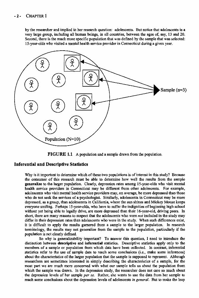
A population is an individual or group that represents all the members of a certain group orcategory of interest. A sample is a subset drawn from the larger population (see Figure 1.1). Forexample, suppose that I wanted to know the average income of the current full-time, tenured facultyat Harvard. There are two ways that I could find this average. First, I could get a list of every full-time, tenured faculty member at Harvard and find out the annual income of each member on this list.Because this list contains every member of the group that I am interested in, it can be considered apopulation. If I were to collect these data and calculate the mean, I would have generated aparameter, because a parameter is a value generated from, or applied to, a population. Another wayto generate the mean income of the tenured faculty at Harvard would be to randomly select a subsetof faculty names from my list and calculate the average income of this subset. The subset is knownas a sample (in this case it is a random sample), and the mean that I generate from this sample is atype of statistic. Statistics are values derived from sample data, whereas parameters are values thatare either derived from, or applied to, population data.
It is important to keep a couple of things in mind about samples and populations. First, apopulation does not need to be large to count as a population. For example, if I wanted to know theaverage height of the students in my statistics class this term, then all of the members of the class(collectively) would comprise the population. If my class only has five students in it, then mypopulation only has five cases. Second, populations (and samples) do not have to include people.For example, suppose I want to know the average age of the dogs that visited a veterinary clinic inthe last year. The population in this study is made up of dogs, not people. Similarly, I may want toknow the total amount of carbon monoxide produced by Ford vehicles that were assembled in theUnited States during 2005. In this example, my population is cars, but not all cars—it is limited toFord cars, and only those actually assembled in a single country during a single calendar year.
Third, the researcher generally defines the population, either explicitly or implicitly. In theexamples above, I defined my populations (of dogs and cars) explicitly. Often, however, researchersdefine their populations less clearly. For example, a researcher may say that the aim of her study isto examine the frequency of depression among adolescents. Her sample, however, may only includea group of 15-year-olds who visited a mental health service provider in Connecticut in a given year.This presents a potential problem, and leads directly into the fourth and final little thing to keep inmind about samples and populations: Samples are not necessarily good representations of thepopulations from which they were selected. In the example about the rates of depression amongadolescents, notice that there are two potential populations. First, there is the population identified
-1-
- 2 - CHAPTER 1
by the researcher and implied in her research question: adolescents. But notice that adolescents is avery large group, including all human beings, in all countries, between the ages of, say, 13 and 20.Second, there is the much more specific population that was defined by the sample that was selected:15-year-olds who visited a mental health service provider in Connecticut during a given year.
FIGURE 1.1 A population and a sample drawn from the population.
Inferential and Descriptive Statistics
Why is it important to determine which of these two populations is of interest in this study? Becausethe consumer of this research must be able to determine how well the results from the samplegeneralize to the larger population. Clearly, depression rates among 15-year-olds who visit mentalhealth service providers in Connecticut may be different from other adolescents. For example,adolescents who visit mental health service providers may, on average, be more depressed than thosewho do not seek the services of a psychologist. Similarly, adolescents in Connecticut may be moredepressed, as a group, than adolescents in California, where the sun shines and Mickey Mouse keepseveryone smiling. Perhaps 15-year-olds, who have to suffer the indignities of beginning high schoolwithout yet being able to legally drive, are more depressed than their 16-year-old, driving peers. Inshort, there are many reasons to suspect that the adolescents who were not included in the study maydiffer in their depression rates than adolescents who were in the study. When such differences exist,it is difficult to apply the results garnered from a sample to the larger population. In researchterminology, the results may not generalize from the sample to the population, particularly if thepopulation is not clearly defined.
So why is generalizability important? To answer this question, I need to introduce thedistinction between descriptive and inferential statistics. Descriptive statistics apply only to themembers of a sample or population from which data have been collected. In contrast, inferentialstatistics refer to the use of sample data to reach some conclusions (i.e., make some inferences)about the characteristics of the larger population that the sample is supposed to represent. Althoughresearchers are sometimes interested in simply describing the characteristics of a sample, for themost part we are much more concerned with what our sample tells us about the population fromwhich the sample was drawn. In the depression study, the researcher does not care so much aboutthe depression levels of her sample per se. Rather, she wants to use the data from her sample toreach some conclusions about the depression levels of adolescents in general. But to make the leap
INTRODUCTION - 3 -
from sample data to inferences about a population, one must be very clear about whether the sampleaccurately represents the population. An important first step in this process is to clearly define thepopulation that the sample is alleged to represent.
SAMPLING ISSUES
There are a number of ways researchers can select samples. One of the most useful, but also themost difficult, is random sampling. In statistics, the term random has a much more specificmeaning than the common usage of the term. It does not mean haphazard. In statistical jargon,random means that every member of a population has an equal chance of being selected into asample. The major benefit of random sampling is that any differences between the sample and thepopulation from which the sample was selected will not be systematic. Notice that in the depressionstudy example, the sample differed from the population in important, systematic (i.e., nonrandom)ways. For example, the researcher most likely systematically selected adolescents who were morelikely to be depressed than the average adolescent because she selected those who had visited mentalhealth service providers. Although randomly selected samples may differ from the larger populationin important ways (especially if the sample is small), these differences are due to chance rather thanto a systematic bias in the selection process.
Representative sampling is a second way of selecting cases for a study. With this method,the researcher purposely selects cases so that they will match the larger population on specificcharacteristics. For example, if I want to conduct a study examining the average annual income ofadults in San Francisco, by definition my population is "adults in San Francisco." This populationincludes a number of subgroups (e.g., different ethnic and racial groups, men and women, retiredadults, disabled adults, parents and single adults, etc.). These different subgroups may be expectedto have different incomes. To get an accurate picture of the incomes of the adult population in SanFrancisco, I may want to select a sample that represents the population well. Therefore, I would tryto match the percentages of each group in my sample that I have in my population. For example, if15% of the adult population in San Francisco is retired, I would select my sample in a manner thatincluded 15% retired adults. Similarly, if 55% of the adult population in San Francisco is male, 55%of my sample should be male. With random sampling, I may get a sample that looks like mypopulation or I may not. But with representative sampling, I can ensure that my sample lookssimilar to my population on some important variables. This type of sampling procedure can becostly and time-consuming, but it increases my chances of being able to generalize the results frommy sample to the population.
Another common method of selecting samples is called convenience sampling. Inconvenience sampling, the researcher generally selects participants on the basis of proximity, ease-of-access, and willingness to participate (i.e., convenience). For example, if I want to do a study onthe achievement levels of eighth-grade students, I may select a sample of 200 students from thenearest middle school to my office. I might ask the parents of 300 of the eighth-grade students in theschool to participate, receive permission from the parents of 220 of the students, and then collectdata from the 200 students that show up at school on the day I hand out my survey. This is aconvenience sample. Although this method of selecting a sample is clearly less labor-intensive thanselecting a random or representative sample, that does not necessary make it a bad way to select asample. If my convenience sample does not differ from my population of interest in ways thatinfluence the outcome of the study, then it is a perfectly acceptable method of selecting a sample.
TYPES OF VARIABLES AND SCALES OF MEASUREMENT
In social science research, a number of terms are used to describe different types of variables. Avariable is pretty much anything that can be codified and have more than a single value (e.g.,income, gender, age, height, attitudes about school, score on a measure of depression, etc.). Aconstant, in contrast, has only a single score. For example, if every member of a sample is male, the"gender" category is a constant. Types of variables include quantitative (or continuous) andqualitative (or categorical). A quantitative variable is one that is scored in such a way that thenumbers, or values, indicate some sort of amount. For example, height is a quantitative (or

- 4 - CHAPTER 1
continuous) variable because higher scores on this variable indicate a greater amount of height. Incontrast, qualitative variables are those for which the assigned values do not indicate more or less ofa certain quality. If I conduct a study to compare the eating habits of people from Maine, NewMexico, and Wyoming, my "state" variable has three values (e.g., 1 = Maine, 2 = New Mexico, 3 =Wyoming). Notice that a value of 3 on this variable is not more than a value of 1 or 2—it is simplydifferent. The labels represent qualitative differences in location, not quantitative differences. Acommonly used qualitative variable in social science research is the dichotomous variable. This isa variable that has two different categories (e.g., male and female).
Most statistics textbooks describe four different scales of measurement for variables:nominal, ordinal, interval, and ratio. A nominally scaled variable is one in which the labels that areused to identify the different levels of the variable have no weight, or numeric value. For example,researchers often want to examine whether men and women differ on some variable (e.g., income).To conduct statistics using most computer software, this gender variable would need to be scoredusing numbers to represent each group. For example, men may be labeled "0" and women may belabeled "1." In this case, a value of 1 does not indicate a higher score than a value of 0. Rather, 0and 1 are simply names, or labels, that have been assigned to each group.
With ordinal variables, the values do have weight. If I wanted to know the 10 richestpeople in America, the wealthiest American would receive a score of 1, the next richest a score of 2,and so on through 10. Notice that while this scoring system tells me where each of the wealthiest 10Americans stands in relation to the others (e.g., Bill Gates is 1, Oprah Winfrey is 8, etc.), it does nottell me how much distance there is between each score. So while I know that the wealthiestAmerican is richer than the second wealthiest, I do not know if he has one dollar more or one billiondollars more. Variables scored using either interval and ratio scales, in contrast, containinformation about both relative value and distance. For example, if I know that one member of mysample is 58 inches tall, another is 60 inches tall, and a third is 66 inches tall, I know who is tallestand how much taller or shorter each member of my sample is in relation to the others. Because myheight variable is measured using inches, and all inches are equal in length, the height variable ismeasured using a scale of equal intervals and provides information about both relative position anddistance. Both interval and ratio scales use measures with equal distances between each unit. Ratioscales also include a zero value (e.g., air temperature using the Celsius scale of measurement).Figure 1.2 provides an illustration of the difference between ordinal and interval/ratio scales ofmeasurement.
FIGURE 1.2 Difference between ordinal and interval/ratio scales of measurement.
INTRODUCTION - 5 -
RESEARCH DESIGNS
There are a variety of research methods and designs employed by social scientists. Sometimesresearchers use an experimental design. In this type of research, the experimenter divides the casesin the sample into different groups and then compares the groups on one or more variables ofinterest. For example, I may want to know whether my newly developed mathematics curriculum isbetter than the old method. I select a sample of 40 students and, using random assignment, teach20 students a lesson using the old curriculum and the other 20 using the new curriculum. Then I testeach group to see which group learned more mathematics concepts. By applying students to the twogroups using random assignment, I hope that any important differences between the two groups getdistributed evenly between the two groups and that any differences in test scores between the twogroups is due to differences in the effectiveness of the two curricula used to teach them. Of course,this may not be true.
Correlational research designs are also a common method of conducting research in thesocial sciences. In this type of research, participants are not usually randomly assigned to groups. Inaddition, the researcher typically does not actually manipulate anything. Rather, the researchersimply collects data on several variables and then conducts some statistical analyses to determinehow strongly different variables are related to each other. For example, I may be interested inwhether employee productivity is related to how much employees sleep (at home, not on the job).So I select a sample of 100 adult workers, measure their productivity at work, and measure how longeach employee sleeps on an average night in a given week. I may find that there is a strongrelationship between sleep and productivity. Now logically, I may want to argue that this makessense, because a more rested employee will be able to work harder and more efficiently. Althoughthis conclusion makes sense, it is too strong a conclusion to reach based on my correlational dataalone. Correlational studies can only tell us whether variables are related to each other—they cannotlead to conclusions about causality. After all, it is possible that being more productive at workcauses longer sleep at home. Getting one's work done may relieve stress and perhaps even allowsthe worker to sleep in a little longer in the morning, both of which create longer sleep.
Experimental research designs are good because they allow the researcher to isolate specificindependent variables that may cause variation, or changes, in dependent variables. In theexample above, I manipulated the independent variable of mathematics curriculum and was able toreasonably conclude that the type of math curriculum used affected students' scores on thedependent variable, test scores. The primary drawbacks of experimental designs are that they areoften difficult to accomplish in a clean way and they often do not generalize to real-world situations.For example, in my study above, I cannot be sure whether it was the math curricula that influencedtest scores or some other factor, such as pre-existing difference in the mathematics abilities of mytwo groups of students or differences in the teacher styles that had nothing to do with the curricula,but could have influenced test scores (e.g., the clarity or enthusiasm of the teacher). The strengths ofcorrelational research designs is that they are often easier to conduct than experimental research,they allow for the relatively easy inclusion of many variables, and they allow the researcher toexamine many variables simultaneously. The principle drawback of correlational research is thatsuch research does not allow for the careful controls necessary for drawing conclusions about causalassociations between variables.
WRAPPING UP AND LOOKING FORWARD
The purpose of this chapter was to provide a quick overview of many of the basic principles andterminology employed in social science research. With a foundation in the types of variables,experimental designs, and sampling methods used in social science research it will be easier tounderstand the uses of the statistics described in the remaining chapters of this book. Now we areready to talk statistics. It may still all be Greek to you, but that's not necessarily a bad thing.

- 6 - CHAPTER 1
GLOSSARY OF TERMS FOR CHAPTER 1
Constant: A construct that has only one value (e.g., if every member of a sample was 10 years old,the "age" construct would be a constant).
Convenience sampling: Selecting a sample based on ease of access or availability.Correlational research design: A style of research used to examine the associations among
variables. Variables are not manipulated by the researcher in this type of research design.Dependent variable: The values of the dependent variable are hypothesized to depend upon the
values of the independent variable. For example, height depends, in part, on gender.Descriptive statistics: Statistics used to described the characteristics of a distribution of scores.Dichotomous variable: A variable that has only two discrete values (e.g., a pregnancy variable can
have a value of 0 for "not pregnant" and 1 for "pregnant."Experimental research design: A type of research in which the experimenter, or researcher,
manipulates certain aspects of the research. These usually include manipulations of theindependent variable and assignment of cases to groups.
Generalize (or Generalizability): The ability to use the results of data collected from a sample toreach conclusions about the characteristics of the population, or any other cases notincluded in the sample.
Independent variable: A variable on which the values of the dependent variable are hypothesizedto depend. Independent variables are often, but not always, manipulated by the researcher.
Inferential statistics: Statistics, derived from sample data, that are used to make inferences aboutthe population from which the sample was drawn.
Interval or Ratio variable: Variables measured with numerical values with equal distance, orspace, between each number (e.g., 2 is twice as much as 1, 4 is twice as much as 2, thedistance between 1 and 2 is the same as the distance between 2 and 3).
Nominally scaled variable: A variable in which the numerical values assigned to each category aresimply labels rather than meaningful numbers.
Ordinal variable: Variables measured with numerical values where the numbers are meaningful(e.g., 2 is larger than 1) but the distance between the numbers is not constant.
Parameter: A value, or values, derived from population data.Population: The collection of cases that comprise the entire set of cases with the specified
characteristics (e.g., all living adult males in the United States).Qualitative (or categorical) variable: A variable that has discrete categories. If the categories are
given numerical values, the values have meaning as nominal references but not asnumerical values (e.g., in 1 = "male" and 2 = "female," 1 is not more or less than 2).
Quantitative (or continuous) variable: A variable that has assigned values and the values areordered and meaningful, such that 1 is less than 2, 2 is less than 3, and so on.
Random assignment: Assignment members of a sample to different groups (e.g., experimental andcontrol) randomly, or without consideration of any of the characteristics of samplemembers.
Random sample (or Random sampling): Selecting cases from a population in a manner thatensures each member of the population has an equal chance of being selected into thesample.
Representative sampling: A method of selecting a sample in which members are purposelyselected to create a sample that represents the population on some characteristic(s) ofinterest (e.g., when a sample is selected to have the same percentages of various ethnicgroups as the larger population).
Sample: A collection of cases selected from a larger population.Statistic: A characteristic, or value, derived from sample data.Variable: Any construct with more than one value that is examined in research.
CHAPTER 2
MEASURES OF CENTRAL TENDENCY
Whenever you collect data, you end up with a group of scores on one or more variables. If you takethe scores on one variable and arrange them in order from lowest to highest, what you get is adistribution of scores. Researchers often want to know about the characteristics of thesedistributions of scores, such as the shape of the distribution, how spread out the scores are, what themost common score is, and so on. One set of distribution characteristics that researchers are usuallyinterested in is central tendency. This set consists of the mean, median, and mode.
The mean is probably the most commonly used statistic in all social science research. Themean is simply the arithmetic average of a distribution of scores, and researchers like it because itprovides a single, simple number that gives a rough summary of the distribution. It is important toremember that although the mean provides a useful piece of information, it does not tell youanything about how spread out the scores are (i.e., variance) or how many scores in the distributionare close to the mean. It is possible for a distribution to have very few scores at or near the mean.
The median is the score in the distribution that marks the 50th percentile. That is, 50%percent of the scores in the distribution fall above the median and 50% fall below it. Researchersoften use the median when they want to divide their distribution scores into two equal groups (calleda median split). The median is also a useful statistic to examine when the scores in a distributionare skewed or when there are a few extreme scores at the high end or the low end of the distribution.This is discussed in more detail in the following pages.
The mode is the least used of the measures of central tendency because it provides the leastamount of information. The mode simply indicates which score in the distribution occurs mostoften, or has the highest frequency.
A Word About Populations and Samples
You will notice in Table 2.1 that there are two different symbols used for the mean, X and u.Two different symbols are needed because it is important to distinguish between a statistic thatapplies to a sample and a parameter that applies to a population. The symbol used to representthe population mean is u. Statistics are values derived from sample data, whereas parameters arevalues that are either derived from, or applied to, population data. It is important to note that allsamples are representative of some population and that all sample statistics can be used as estimatesof population parameters. In the case of the mean, the sample statistic is represented with thesymbol X. The distinction between sample statistics and population parameters appears in severalchapters (e.g., Chapters 1, 3, 5, and 7).
MEASURES OF CENTRAL TENDENCY IN DEPTH
The calculations for each measure of central tendency are mercifully straightforward. With the aidof a calculator or statistics software program, you will probably never need to calculate any of thesestatistics by hand. But for the sake of knowledge and in the event you find yourself without acalculator and in need of these statistics, here is the information you will need.
Because the mean is an average, calculating the mean involves adding, or summing, all ofthe scores in a distribution and dividing by the number of scores. So, if you have 10 scores in adistribution, you would add all of the scores together to find the sum and then divide the sum by 10,
-7-

-8- CHAPTER 2
which is the number of scores in the distribution. The formula for calculating the mean is presentedin Table 2.1.
TABLE 2.1 Formula for calculating the mean of a distribution.
or
where X is the sample meanu is the population mean
E means "the sum ofX is an individual score in the distributionn is the number of scores in the sampleN is the number of scores in the population
The calculation of the median (P5o) for a simple distribution of scores1 is even simpler thanthe calculation of the mean. To find the median of a distribution, you need to first arrange all of thescores in the distribution in order, from smallest to largest. Once this is done, you simply need tofind the middle score in the distribution. If there is an odd number of scores in the distribution, therewill be a single score that marks the middle of the distribution. For example, if there are 11 scores inthe distribution arranged in descending order from smallest to largest, the 6th score will be themedian because there will be 5 scores below it and 5 scores above it. However, if there are an evennumber of scores in the distribution, there is no single middle score. In this case, the median is theaverage of the two scores in the middle of the distribution (as long as the scores are arranged inorder, from largest to smallest). For example, if there are 10 scores in a distribution, to find themedian you will need to find the average of the 5th and 6th scores. To find this average, add the twoscores together and divide by two.
To find the mode, there is no need to calculate anything. The mode is simply thecategory in the distribution that has the highest number of scores, or the highest frequency. Forexample, suppose you have the following distribution of IQ test scores from 10 students:
86 90 95 100 100 100 110 110 115 120
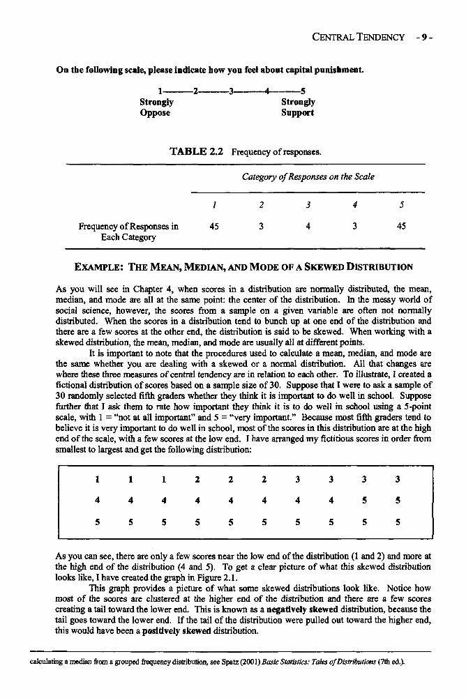
In this distribution, the score that occurs most frequently is 100, making it the mode of thedistribution. If a distribution has more than one category with the most common score, thedistribution has multiple modes and is called multimodal. One common example of a multimodaldistribution is the bimodal distribution. Researchers often get bimodal distributions when they askpeople to respond to controversial questions that tend to polarize the public. For example, if I wereto ask a sample of 100 people how they feel about capital punishment, I might get the resultspresented in Table 2.2. In this example, because most people either strongly oppose or stronglysupport capital punishment, I end up with a bimodal distribution of scores.
1 It is also possible to calculate the median of a grouped frequency distribution. For an excellent description of the technique for
CENTRAL TENDENCY - 9 -
On the following scale, please indicate how you feel about capital punishment.
TABLE 2.2 Frequency of responses.
Category of Responses on the Scale
1
45
2
3
3
4
4
3
5
45Frequency of Responses inEach Category
EXAMPLE: THE MEAN, MEDIAN, AND MODE OF A SKEWED DISTRIBUTION
As you will see in Chapter 4, when scores in a distribution are normally distributed, the mean,median, and mode are all at the same point: the center of the distribution. In the messy world ofsocial science, however, the scores from a sample on a given variable are often not normallydistributed. When the scores in a distribution tend to bunch up at one end of the distribution andthere are a few scores at the other end, the distribution is said to be skewed. When working with askewed distribution, the mean, median, and mode are usually all at different points.
It is important to note that the procedures used to calculate a mean, median, and mode arethe same whether you are dealing with a skewed or a normal distribution. All that changes arewhere these three measures of central tendency are in relation to each other. To illustrate, I created afictional distribution of scores based on a sample size of 30. Suppose that I were to ask a sample of30 randomly selected fifth graders whether they think it is important to do well in school. Supposefurther that I ask them to rate how important they think it is to do well in school using a 5-pointscale, with 1 = "not at all important" and 5 = "very important." Because most fifth graders tend tobelieve it is very important to do well in school, most of the scores in this distribution are at the highend of the scale, with a few scores at the low end. I have arranged my fictitious scores in order fromsmallest to largest and get the following distribution:
1
4
5
1
4
5
1
4
5
2
4
5
2
4
5
2
4
5
3
4
5
3
4
5
3
5
5
3
5
5
As you can see, there are only a few scores near the low end of the distribution (1 and 2) and more atthe high end of the distribution (4 and 5). To get a clear picture of what this skewed distributionlooks like, I have created the graph in Figure 2.1.
This graph provides a picture of what some skewed distributions look like. Notice howmost of the scores are clustered at the higher end of the distribution and there are a few scorescreating a tail toward the lower end. This is known as a negatively skewed distribution, because thetail goes toward the lower end. If the tail of the distribution were pulled out toward the higher end,this would have been a positively skewed distribution.
calculating a median from a grouped frequency distribution, see Spatz (2001) Basic Statistics: Tales of Distributions (7th ed.).

-10 - CHAPTER 2
A quick glance at the scores in the distribution, or at the graph, reveals that the mode is 5because there were more scores of 5 than any other number in the distribution.
To calculate the mean, we simply apply the formula mentioned earlier. That is, we add upall of the scores (EX) and then divide this sum by the number of scores in the distribution (n). Thisgives us a fraction of 113/30, which reduces to 3.7666. When we round to the second place after thedecimal, we end up with a mean of 3.77.
FIGURE 2.1 A skewed distribution.
To find the median of this distribution, we arrange the scores in order from smallest tolargest and find the middle score. In this distribution, there are 30 scores, so there will be 2 in themiddle. When arranged in order, the 2 scores in the middle (the 15th and 16th scores) are both 4.When we add these two scores together and divide by 2, we end up with 4, making our median 4.
As I mentioned earlier, the mean of a distribution can be affected by scores that areunusually large or small for a distribution, sometimes called outliers, whereas the median is notaffected by such scores. In the case of a skewed distribution, the mean is usually pulled in thedirection of the tail, because the tail is where the outliers are. In a negatively skewed distribution,such as the one presented previously, we would expect the mean to be smaller than the median,because the mean is pulled toward the tail whereas the median is not. In our example, the mean(3.77) is somewhat lower than the median (4). In positively skewed distributions, the mean issomewhat higher than the median.
WRAPPING UP AND LOOKING FORWARD
Measures of central tendency, particularly the mean and the median, are some of the most used anduseful statistics for researchers. They each provide important information about an entiredistribution of scores in a single number. For example, we know that the average height of a man inthe United States is five feet nine inches tall. This single number is used to summarize informationabout millions of men in this country. But for the same reason that the mean and median are useful,they can often be dangerous if we forget that a statistic such as the mean ignores a lot of informationabout a distribution, including the great amount of variety that exists in many distributions. Withoutconsidering the variety as well as the average, it becomes easy to make sweeping generalizations, orstereotypes, based on the mean. The measure of variance is the topic of the next chapter.
CENTRAL TENDENCY -11 -
GLOSSARY OF TERMS AND SYMBOLS FOR CHAPTER 2
Bimodal: A distribution that has two values that have the highest frequency of scores.Distribution: A collection, or group, of scores from a sample on a single variable. Often, but not
necessarily, these scores are arranged in order from smallest to largest.Mean: The arithmetic average of a distribution of scores.Median split: Dividing a distribution of scores into two equal groups by using the median score as
the divider. Those scores above the median are the "high" group whereas those below themedian are the "low" group.
Median: The score in a distribution that marks the 50th percentile. It is the score at which 50% ofthe distribution falls below and 50% fall above.
Mode: The score in the distribution that occurs most frequently.Multimodal: When a distribution of scores has two or more values that have the highest frequency
of scores.Negative skew: In a skewed distribution, when most of the scores are clustered at the higher end of
the distribution with a few scores creating a tail at the lower end of the distribution.Outliers: Extreme scores that are more than two standard deviations above or below the mean.Positive skew: In a skewed distribution, when most of the scores are clustered at the lower end of
the distribution with a few scores creating a tail at the higher end of the distribution.Parameter: A value derived from the data collected from a population, or the value inferred to the
population from a sample statistic.Population: The group from which data are collected or a sample is selected. The population
encompasses the entire group for which the data are alleged to apply.Sample: An individual or group, selected from a population, from whom or which data are
collected.Skew: When a distribution of scores has a high number of scores clustered at one end of the
distribution with relatively few scores spread out toward the other end of the distribution,forming a tail.
Statistic: A value derived from the data collected from a sample.
£ The sum of; to sum.X An individual score in a distribution.EX The sum of X; adding up all of the scores in a distribution.
X The mean of a sample.u The mean of a population.n The number of cases, or scores, in a sample.N The number of cases, or scores, in a population.P50 Symbol for the median.

This page intentionally left blank

CHAPTER 3
MEASURES OF VARIABILITY
Measures of central tendency, such as the mean and the median described in Chapter 2, provideuseful information. But it is important to recognize that these measures are limited and, bythemselves, do not provide a great deal of information. There is an old saying that provides acaution about the mean: "If your head is in the freezer and your feet are in the oven, on averageyou're comfortable." To illustrate, consider this example: Suppose I gave a sample of 100 fifth-grade children a survey to assess their level of depression. Suppose further that this sample had amean of 10.0 on my depression survey and a median of 10.0 as well. All we know from thisinformation is that the mean and median are in the same place in my distribution, and this place is10.0. Now consider what we do not know. We do not know if this is a high score or a low score.We do not know if all of the students in my sample have about the same level of depression or ifthey differ from each other. We do not know the highest depression score in our distribution or thelowest score. Simply put, we do not yet know anything about the dispersion of scores in thedistribution. In other words, we do not yet know anything about the variety of the scores in thedistribution.
There are three measures of dispersion that researchers typically examine: the range, thevariance, and the standard deviation. Of these, the standard deviation is perhaps the mostinformative and certainly the most widely used.
Range
The range is simply the difference between the largest score (the maximum value) and the smallestscore (the minimum value) of a distribution. This statistic gives researchers a quick sense of howspread out the scores of a distribution are, but it is not a particularly useful statistic because it can bequite misleading. For example, in our depression survey described earlier, we may have 1 studentscore a 1 and another score a 20, but the other 98 may all score 10. In this example, the range willbe 19 (20 - 1 = 19), but the scores really are not as spread out as the range might suggest.Researchers often take a quick look at the range to see whether all or most of the points on a scale,such as a survey, were covered in the sample.
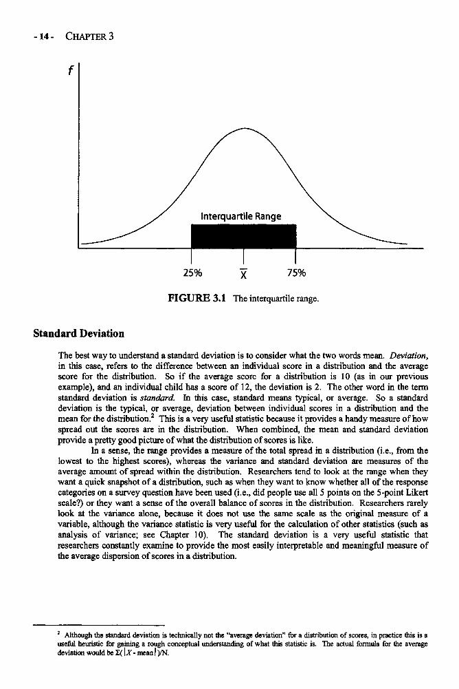
Another common measure of the range of scores in a distribution is the interquartile range(IQR). Unlike the range, which is the difference between the largest and smallest score in thedistribution, the IQR is the difference between the score that marks the 75th percentile (the thirdquartile) and the score that marks the 25th percentile (the first quartile). If the scores in adistribution were arranged in order from largest to smallest and then divided into groups of equalsize, the IQR would contain the scores in the two middle quartiles (see Figure 3.1).
Variance
The variance provides a statistical average of the amount of dispersion in a distribution of scores.Because of the mathematical manipulation needed to produce a variance statistic (more about this inthe next section), variance, by itself, is not often used by researchers to gain a sense of a distribution.In general, variance is used more as a step in the calculation of other statistics (e.g., analysis ofvariance) than as a stand-alone statistic. But with a simple manipulation, the variance can betransformed into the standard deviation, which is one of the statistician's favorite tools.
-13-
-14 - CHAPTER 3
FIGURE 3.1 The interquartile range.
Standard Deviation
The best way to understand a standard deviation is to consider what the two words mean. Deviation,in this case, refers to the difference between an individual score in a distribution and the averagescore for the distribution. So if the average score for a distribution is 10 (as in our previousexample), and an individual child has a score of 12, the deviation is 2. The other word in the termstandard deviation is standard. In this case, standard means typical, or average. So a standarddeviation is the typical, or average, deviation between individual scores in a distribution and themean for the distribution.2 This is a very useful statistic because it provides a handy measure of howspread out the scores are in the distribution. When combined, the mean and standard deviationprovide a pretty good picture of what the distribution of scores is like.
In a sense, the range provides a measure of the total spread in a distribution (i.e., from thelowest to the highest scores), whereas the variance and standard deviation are measures of theaverage amount of spread within the distribution. Researchers tend to look at the range when theywant a quick snapshot of a distribution, such as when they want to know whether all of the responsecategories on a survey question have been used (i.e., did people use all 5 points on the 5-point Likertscale?) or they want a sense of the overall balance of scores in the distribution. Researchers rarelylook at the variance alone, because it does not use the same scale as the original measure of avariable, although the variance statistic is very useful for the calculation of other statistics (such asanalysis of variance; see Chapter 10). The standard deviation is a very useful statistic thatresearchers constantly examine to provide the most easily interpretable and meaningful measure ofthe average dispersion of scores in a distribution.
2 Although the standard deviation is technically not the "average deviation" for a distribution of scores, in practice this is auseful heuristic for gaining a rough conceptual understanding of what this statistic is. The actual formula for the averagedeviation would be E( |X - mean | )/N.
VARIABILITY - 15 -
MEASURES OF VARIABILITY IN DEPTH
Calculating the Variance and Standard Deviation
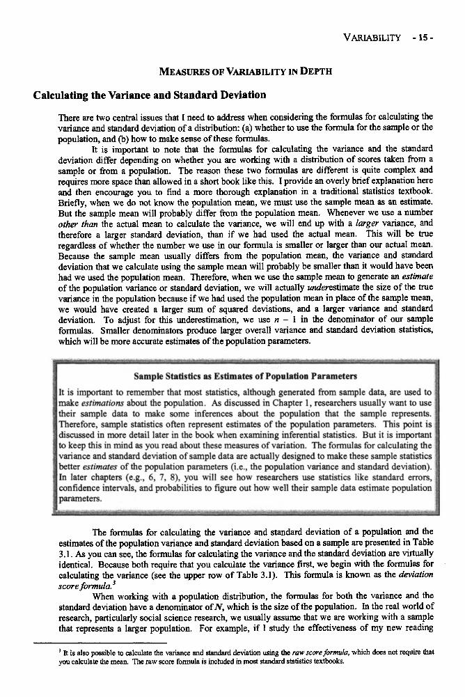
There are two central issues that I need to address when considering the formulas for calculating thevariance and standard deviation of a distribution: (a) whether to use the formula for the sample or thepopulation, and (b) how to make sense of these formulas.
It is important to note that the formulas for calculating the variance and the standarddeviation differ depending on whether you are working with a distribution of scores taken from asample or from a population. The reason these two formulas are different is quite complex andrequires more space than allowed in a short book like this. I provide an overly brief explanation hereand then encourage you to find a more thorough explanation in a traditional statistics textbook.Briefly, when we do not know the population mean, we must use the sample mean as an estimate.But the sample mean will probably differ from the population mean. Whenever we use a numberother than the actual mean to calculate the variance, we will end up with a larger variance, andtherefore a larger standard deviation, than if we had used the actual mean. This will be trueregardless of whether the number we use in our formula is smaller or larger than our actual mean.Because the sample mean usually differs from the population mean, the variance and standarddeviation that we calculate using the sample mean will probably be smaller than it would have beenhad we used the population mean. Therefore, when we use the sample mean to generate an estimateof the population variance or standard deviation, we will actually underestimate the size of the truevariance in the population because if we had used the population mean in place of the sample mean,we would have created a larger sum of squared deviations, and a larger variance and standarddeviation. To adjust for this underestimation, we use n - 1 in the denominator of our sampleformulas. Smaller denominators produce larger overall variance and standard deviation statistics,which will be more accurate estimates of the population parameters.
Sample Statistics as Estimates of Population Parameters
It is important to remember that most statistics, although generated from sample data, are used tomake estimations about the population. As discussed in Chapter 1, researchers usually want to usetheir sample data to make some inferences about the population that the sample represents.Therefore, sample statistics often represent estimates of the population parameters. This point isdiscussed in more detail later in the book when examining inferential statistics. But it is importantto keep this in mind as you read about these measures of variation. The formulas for calculating thevariance and standard deviation of sample data are actually designed to make these sample statisticsbetter estimates of the population parameters (i.e., the population variance and standard deviation).In later chapters (e.g., 6, 7, 8), you will see how researchers use statistics like standard errors,confidence intervals, and probabilities to figure out how well their sample data estimate populationparameters.
The formulas for calculating the variance and standard deviation of a population and theestimates of the population variance and standard deviation based on a sample are presented in Table3.1. As you can see, the formulas for calculating the variance and the standard deviation are virtuallyidentical. Because both require that you calculate the variance first, we begin with the formulas forcalculating the variance (see the upper row of Table 3.1). This formula is known as the deviationscore formula.3
When working with a population distribution, the formulas for both the variance and thestandard deviation have a denominator of N, which is the size of the population. In the real world ofresearch, particularly social science research, we usually assume that we are working with a samplethat represents a larger population. For example, if I study the effectiveness of my new reading
3 It is also possible to calculate the variance and standard deviation using the raw score formula, which does not require thatyou calculate the mean. The raw score formula is included in most standard statistics textbooks.
-16 - CHAPTER 3
program with a class of second graders, as a researcher I assume that these particular second gradersrepresent a larger population of second graders, or students more generally. Because of this type ofinference, researchers generally think of their research participants as a sample rather than apopulation, and the formula for calculating the variance of a sample is the formula more often used.Notice that the formula for calculating the variance of a sample is identical to that used for thepopulation, except the denominator for the sample formula is n - 1.
How much of a difference does it make if we use N or n - 1 in our denominator? Well, thatdepends on the size of the sample. If we have a sample of 500 people, there is virtually nodifference between the variance formula for the population and for the estimate based on the sample.After all, dividing a numerator by 500 is almost the same as dividing it by 499. But when we have asmall sample, such as a sample of 10, then there is a relatively large difference between the resultsproduced by the population and sample formulas.
TABLE 3.1 Variance and standard deviation formulas.
Population Estimate Based on a Sample
Variance
where 2 = to sumX- a score in the distributionu = the population meanN = the number of cases in the
population
where £ = to sumX = a score in the distributionX = the sample meann = the number of cases in the
sample
Standard Deviation
where E = to sumX- a score in the distributionu. = the population meanN - the number of cases in the
Population
where E = to sumX- a score in the distributionX = the sample meann = the number of cases in the
sample
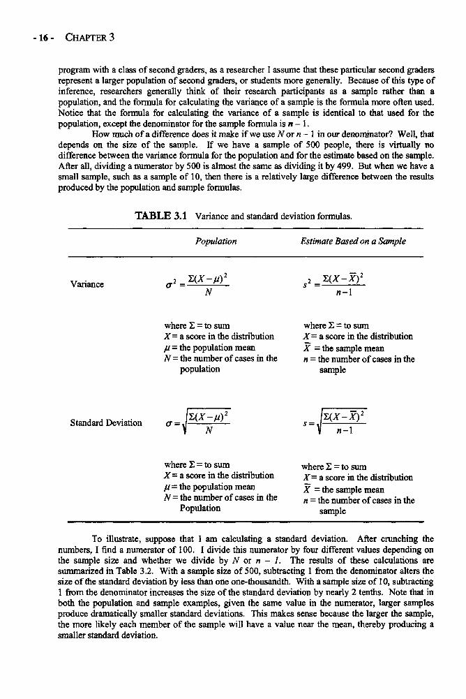
To illustrate, suppose that I am calculating a standard deviation. After crunching thenumbers, I find a numerator of 100. I divide this numerator by four different values depending onthe sample size and whether we divide by N or n - 1. The results of these calculations aresummarized in Table 3.2. With a sample size of 500, subtracting 1 from the denominator alters thesize of the standard deviation by less than one one-thousandth. With a sample size of 10, subtracting1 from the denominator increases the size of the standard deviation by nearly 2 tenths. Note that inboth the population and sample examples, given the same value in the numerator, larger samplesproduce dramatically smaller standard deviations. This makes sense because the larger the sample,the more likely each member of the sample will have a value near the mean, thereby producing asmaller standard deviation.
VARIABILITY -17 -
TABLE 3.2 Effects of sample size and n -1 on standard deviation.
Population
Sample
The second issue to address involves making sense of the formulas for calculating thevariance. In all honesty, there will be very few times that you will need to use this formula. Outsideof my teaching duties, I haven't calculated a standard deviation by hand since my first statisticscourse. Thankfully, all computer statistics and spreadsheet programs, and many calculators,compute the variance and standard deviation for us. Nevertheless, it is mildly interesting and quiteinformative to examine how these variance formulas work.
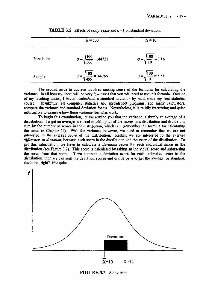
To begin this examination, let me remind you that the variance is simply an average of adistribution. To get an average, we need to add up all of the scores in a distribution and divide thissum by the number of scores in the distribution, which is n (remember the formula for calculatingthe mean in Chapter 2?). With the variance, however, we need to remember that we are notinterested in the average score of the distribution. Rather, we are interested in the averagedifference, or deviation, between each score in the distribution and the mean of the distribution. Toget this information, we have to calculate a deviation score for each individual score in thedistribution (see Figure 3.2). This score is calculated by taking an individual score and subtractingthe mean from that score. If we compute a deviation score for each individual score in thedistribution, then we can sum the deviation scores and divide by n to get the average, or standard,deviation, right? Not quite.
FIGURE 3.2 A deviation.
- 18 - CHAPTER 3
The problem here is that, by definition, the mean of a distribution is the mathematicalmiddle of the distribution. Therefore, some of the scores in the distribution will fall above the mean(producing positive deviation scores), and some will fall below the mean (producing negativedeviation scores). When we add these positive and negative deviation scores together, the sum willbe zero. Because the mean is the mathematical middle of the distribution, we will get zero when weadd up these deviation scores no matter how big or small our sample, or how skewed or normal ourdistribution. And because we cannot find an average of zero (i.e., zero divided by n is zero, nomatter what n is), we need to do something to get rid of this zero.
The solution statisticians came up with is to make each deviation score positive by squaringit. So, for each score in a distribution, we subtract the mean of the distribution and then square thedeviation. If you look at the deviation score formulas in Table 3.1, you will see that all that theformula is doing with (X - u)2 is to take each score, subtract the mean, and square the resultingdeviation score. What you get when you do this is the all-important squared deviation, which isused all the time in statistics. If we then put a summation sign in front, we have E ( X - u)2. What thistells us is that after we produce a squared deviation score for each case in our distribution, we thenneed to add up all of these squared deviations, giving us the sum of squared deviations, or the sumof squares (SS). Once this is done, we divide by the number of cases in our distribution, and we getan average, or mean, of the squared deviations. This is our variance.
The final step in this process is converting the variance into a standard deviation.Remember that in order to calculate the variance, we have to square each deviation score. We dothis to avoid getting a sum of zero in our numerator. When we square these scores, we change ourstatistic from our original scale of measurement (i.e., whatever units of measurement were used togenerate our distribution of scores) to a squared score. To reverse this process and give us a statisticthat is back to our original unit of measurement, we merely need to take the square root of ourvariance. When we do this, we switch from the variance to the standard deviation. Therefore, theformula for calculating the standard deviation is exactly the same as the formula for calculating thevariance, except we put a big square root symbol over the whole formula. Notice that because of thesquaring and square rooting process, the standard deviation and the variance are always positivenumbers.
Why Have Variance?
If the variance is a difficult statistic to understand, and rarely examined by researchers, why not justeliminate this statistic and jump straight to the standard deviation? There are two reasons. First, weneed to calculate the variance before we can find the standard deviation anyway, so it is not morework. Second, the fundamental piece of the variance formula, which is the sum of the squareddeviations, is used in a number of other statistics, most notably analysis of variance (ANOVA).When you learn about more advanced statistics such as ANOVA (Chapter 10), factorial ANOVA(Chapter 11), and even regression (Chapter 13), you will see that each of these statistics uses the sumof squares, which is just another way of saying the sum of the squared deviations. Because the sumof squares is such an important piece of so many statistics, the variance statistic has maintained aplace in the teaching of basic statistics.
EXAMPLE: EXAMINING THE RANGE, VARIANCE, AND STANDARD DEVIATION
I conducted a study in which I gave questionnaires to approximately 500 high school students in the9th and llth grades. In the examples that follow, we examine the mean, range, variance, andstandard deviation of the distribution of responses to two of these questions. To make sense of these(and all) statistics, you need to know the exact wording of the survey items and the response scaleused to answer the survey items. Although this may sound obvious, I mention it here because, if younotice, much of the statistical information reported in the news (e.g., the results of polls) does notprovide the exact wording of the questions or the response choices. Without this information, it isdifficult to know exactly what the responses mean, and "lying with statistics" becomes easier.
The first survey item we examine reads, "If I have enough time, I can do even the mostdifficult work in this class." This item is designed to measure students' confidence in their abilities
VARIABILITY -19 -
to succeed in their classwork. Students were asked to respond to this question by circling a numberon a scale from 1 to 5. On this scale, circling the 1 means that the statement is "not at all true" andthe 5 means "very true." So students were basically asked to indicate how true they felt thestatement was on a scale from 1 to 5, with higher numbers indicating a stronger belief that thestatement was true.
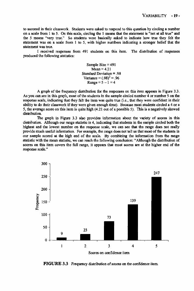
I received responses from 491 students on this item. The distribution of responsesproduced the following statistics:
Sample Size = 491Mean = 4.21
Standard Deviation = .98Variance = (.98)2 = .96
Range = 5 - 1 = 4
A graph of the frequency distribution for the responses on this item appears in Figure 3.3.As you can see in this graph, most of the students in the sample circled number 4 or number 5 on theresponse scale, indicating that they felt the item was quite true (i.e., that they were confident in theirability to do their classwork if they were given enough time). Because most students circled a 4 or a5, the average score on this item is quite high (4.21 out of a possible 5). This is a negatively skeweddistribution.
The graph in Figure 3.3 also provides information about the variety of scores in thisdistribution. Although our range statistic is 4, indicating that students in the sample circled both thehighest and the lowest number on the response scale, we can see that the range does not reallyprovide much useful information. For example, the range does not tell us that most of the students inour sample scored at the high end of the scale. By combining the information from the rangestatistic with the mean statistic, we can reach the following conclusion: "Although the distribution ofscores on this item covers the full range, it appears that most scores are at the higher end of theresponse scale."
FIGURE 3.3 Frequency distribution of scores on the confidence item.
- 20 - CHAPTER 3
Now that we've determined that (a) the distribution of scores covers the full range ofpossible scores (i.e., from 1 to 5), and (b) most of the responses are at the high end of the scale(because the mean is 4.21 out of a possible 5), we may want a more precise measure of the averageamount of variety among the scores in the distribution. For this we turn to the variance and standarddeviation statistics. In this example, the variance (.96) is almost exactly the same as the standarddeviation (.98). This is something of a fluke. Do not be fooled. It is quite rare for the variance andstandard deviation to be so similar. In fact, this only happens if the standard deviation is about 1.0,because 1.0 squared is 1.0. So in this rare case, the variance and standard deviation provide almostthe same information. Namely, they indicate that the average difference between an individual scorein the distribution and the mean for the distribution is about 1 point on the 5-point scale.
Taken together, these statistics tell us the same things that the graph tells us, but moreprecisely. Namely, we now know that (a) students in the study answered this item covering thewhole range of response choices (i.e., 1 - 5); (b) most of the students answered at or near the top ofthe range, because the mean is quite high; and (c) the scores in this distribution generally pack fairlyclosely together with most students having circled a number within 1 point of the mean, because thestandard deviation was .98. The variance tells us that the average squared deviation is .96, and wescratch our heads, wonder what good it does us to know the average squared deviation, and move on.
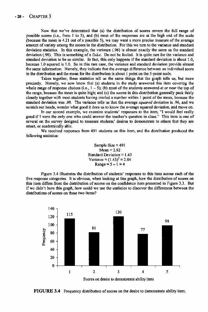
In our second example, we examine students' responses to the item, "I would feel reallygood if I were the only one who could answer the teacher's question in class." This item is one ofseveral on the survey designed to measure students' desires to demonstrate to others that they aresmart, or academically able.
We received responses from 491 students on this item, and the distribution produced thefollowing statistics:
Sample Size = 491Mean = 2.92
Standard Deviation = 1.43Variance = (1.43)2 = 2.04
Range = 5 -1=4
Figure 3.4 illustrates the distribution of students' responses to this item across each of thefive response categories. It is obvious, when looking at this graph, how the distribution of scores onthis item differs from the distribution of scores on the confidence item presented in Figure 3.3. Butif we didn't have this graph, how could we use the statistics to discover the differences between thedistributions of scores on these two items?
FIGURE 3.4 Frequency distribution of scores on the desire to demonstrate ability item.
VARIABILITY - 21 -
Notice that, as with the previous item, the range is 4, indicating that some students circledthe number 1 on the response scale and some circled the number 5. Because the ranges for both theconfidence and the wanting to appear able items are equal (i.e., 4), they do nothing to indicate thedifferences in the distributions of the responses to these two items. That is why the range is not aparticularly useful statistic—it simply does not provide very much information.
Our first real indication that the distributions differ substantially comes from a comparisonof the means. In the previous example, the mean of 4.21 indicated that most of the students musthave circled either a 4 or a 5 on the response scale. For this second item, the mean of 2.92 is a bitless informative. Although it provides an average score, it is impossible from just examining themean to determine whether most students circled a 2 or 3 on the scale, or whether roughly equalnumbers of students circled each of the five numbers on the response scale, or whether almost half ofthe students circled 1 whereas the other half circled 5. All three scenarios would produce a mean ofabout 2.92, because that is roughly the middle of the response scale.
To get a better picture of this distribution, we need to consider the standard deviation inconjunction with the mean. Before discussing the actual standard deviation for this distribution ofscores, let us briefly consider what we would expect the standard deviation to be for each of thethree scenarios just described. First, if almost all of the students circled a 2 or a 3 on the responsescale, we would expect a fairly small standard deviation, as we saw in the previous example usingthe confidence item. The more similar the responses are to an item, the smaller the standarddeviation. However, if half of the students circled 1 and the other half circled 5, we would expect alarge standard deviation (about 2.0) because each score would be about two units away from themean i.e., if the mean is about 3.0 and each response is either 1 or 5, each response is about two unitsaway from the mean. Finally, if the responses are fairly evenly spread out across the five responsecategories, we would expect a moderately sized standard deviation (about 1.50).
Now, when we look at the actual mean for this distribution (2.92) and the actual standarddeviation (1.43), we can develop a rough picture of the distribution in our minds. Because we knowthat on a scale from 1 to 5, a mean of 2.92 is about in the middle, we can guess that the distributionlooks somewhat symmetrical (i.e., that there will be roughly the same number of responses in the 4and 5 categories as there are in the 1 and 2 categories. Furthermore, because we've got a moderatelysized standard deviation of 1.43, we know that the scores are pretty well spread out, with a healthynumber of students in each of the five response categories. So we know that we didn't get anoverwhelming number of students circling 3 and we didn't get students circling only 1 or 5. At thispoint, this is about all we can say about this distribution: The mean is near the middle of the scale,and the responses are pretty well spread out across the five response categories. To say any more,we would need to look at the number of responses in each category, such as that presented in Figure3.4.
As we look at the actual distribution of scores presented in the graph in Figure 3.4, we cansee that the predictions we generated from our statistics about the shape of the distribution are prettyaccurate. Notice that we did not need to consider the variance at all, because the variance in thisexample (2.04) is on a different scale of measurement than our original 5-point response scale, andtherefore is very difficult to interpret. Variance is an important statistic for many techniques (e.g.,ANOVA, regression), but it does little to help us understand the shape of a distribution of scores.The mean, standard deviation, and to a lesser extent the range, when considered together, canprovide a rough picture of a distribution of scores. Often, a rough picture is all a researcher needs orwants. Sometimes, however, researchers need to know more precisely the characteristics of adistribution of scores. In that case, a picture, such as a graph, may be worth a thousand words.
Another useful way to examine a distribution of scores is to create a boxplot. In Figure 3.5,a boxplot is presented for the same variable that is represented in Figure 3.4, wanting to demonstrateability. This boxplot was produced in the SPSS statistical software program. The box in this graphcontains some very useful information. First, the thick line in the middle of the box represents themedian of this distribution of scores. The top line of the box represents the 75th percentile of thedistribution and the bottom line represents the 25th percentile. Therefore, the top and bottom linesof the box reveal the interquartile range (IQR) for this distribution. In other words, 50% of thescores on this variable in this distribution are contained within the upper and lower lines of this box(i.e., 50% of the scores are between just above a score of 2 and just below a score of 4). The vertical

- 22 - CHAPTER 3
lines coming out of the top and bottom of the box and culminating in horizontal lines reveal thelargest and smallest scores in the distribution, or the range. These scores are 5 and 1, producing arange of 5 - 1 = 4. As you can see, the boxplot in Figure 3.5 contains a lot of useful informationabout the spread of scores on this variable in a single picture.
FIGURE 3.5 Boxplot for the desire to appear able variable.
WRAPPING UP AND LOOKING FORWARD
Measures of variation, such as the variance, standard deviation, and range, are important descriptivestatistics. They provide useful information about how spread out the scores of a distribution are, andthe shape of the distribution. Perhaps even more important than their utility as descriptors of a singledistribution of scores is their role in more advanced statistics such as those coming in later chapters(e.g., ANOVA in Chapters 10, 11, and 12). In the next chapter, we examine the properties of atheoretical distribution, the normal distribution, that has a specific shape and characteristics. Usingsome of the concepts from Chapter 3, we can see how the normal distribution can be used to makeinferences about the population based on sample data.
GLOSSARY OF TERMS AND SYMBOLS FOR CHAPTER 3
Boxplot: A graphic representation of the distribution of scores on a variable that includes the range,the median, and the interquartile range.
Interquartile range (IQR): The difference between the 75th percentile and 25th percentile scores ina distribution.
Range: The difference between the largest score and the smallest score of a distribution.Squared deviation: The difference between an individual score in a distribution and the mean for
the distribution, squared.Standard deviation: The average deviation between the individual scores in the distribution and
the mean for the distribution.

VARIABILITY - 23 -
Sum of squared deviations, sum of squares: The sum of each squared deviation for all of thecases in the sample.
Variance: The sum of the squared deviations divided by the number of cases in the population, orby the number of cases minus one in the sample.
u The population mean.X An individual score in a distribution.s2 The sample variance.s The sample standard deviation.o The population standard deviation.o The population variance.SS The sum of squares, or sum of squared deviations.n The number of cases in the sample.N The number of cases in the population.

This page intentionally left blank
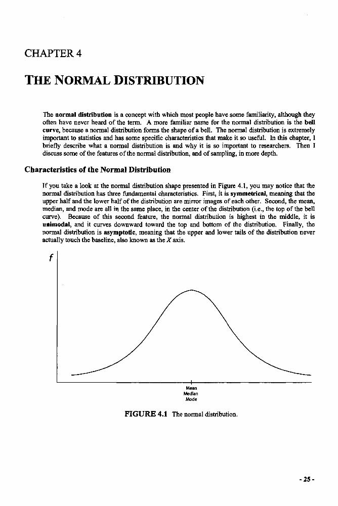
CHAPTER 4
THE NORMAL DISTRIBUTION
The normal distribution is a concept with which most people have some familiarity, although theyoften have never heard of the term. A more familiar name for the normal distribution is the bellcurve, because a normal distribution forms the shape of a bell. The normal distribution is extremelyimportant to statistics and has some specific characteristics that make it so useful. In this chapter, Ibriefly describe what a normal distribution is and why it is so important to researchers. Then Idiscuss some of the features of the normal distribution, and of sampling, in more depth.
Characteristics of the Normal Distribution
If you take a look at the normal distribution shape presented in Figure 4.1, you may notice that thenormal distribution has three fundamental characteristics. First, it is symmetrical, meaning that theupper half and the lower half of the distribution are mirror images of each other. Second, the mean,median, and mode are all in the same place, in the center of the distribution (i.e., the top of the bellcurve). Because of this second feature, the normal distribution is highest in the middle, it isunimodal, and it curves downward toward the top and bottom of the distribution. Finally, thenormal distribution is asymptotic, meaning that the upper and lower tails of the distribution neveractually touch the baseline, also known as the X axis.
FIGURE 4.1 The normal distribution.
-25-
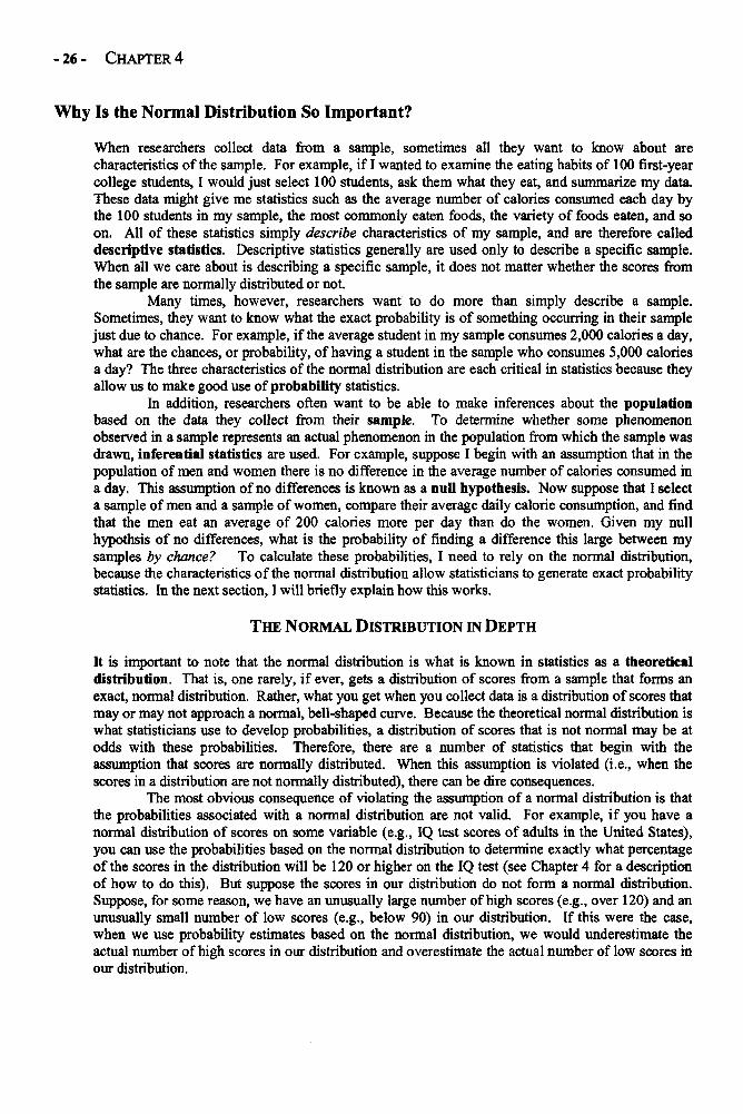
-26- CHAPTER 4
Why Is the Normal Distribution So Important?
When researchers collect data from a sample, sometimes all they want to know about arecharacteristics of the sample. For example, if I wanted to examine the eating habits of 100 first-yearcollege students, I would just select 100 students, ask them what they eat, and summarize my data.These data might give me statistics such as the average number of calories consumed each day bythe 100 students in my sample, the most commonly eaten foods, the variety of foods eaten, and soon. All of these statistics simply describe characteristics of my sample, and are therefore calleddescriptive statistics. Descriptive statistics generally are used only to describe a specific sample.When all we care about is describing a specific sample, it does not matter whether the scores fromthe sample are normally distributed or not.
Many times, however, researchers want to do more than simply describe a sample.Sometimes, they want to know what the exact probability is of something occurring in their samplejust due to chance. For example, if the average student in my sample consumes 2,000 calories a day,what are the chances, or probability, of having a student in the sample who consumes 5,000 caloriesa day? The three characteristics of the normal distribution are each critical in statistics because theyallow us to make good use of probability statistics.
In addition, researchers often want to be able to make inferences about the populationbased on the data they collect from their sample. To determine whether some phenomenonobserved in a sample represents an actual phenomenon in the population from which the sample wasdrawn, inferential statistics are used. For example, suppose I begin with an assumption that in thepopulation of men and women there is no difference in the average number of calories consumed ina day. This assumption of no differences is known as a null hypothesis. Now suppose that I selecta sample of men and a sample of women, compare their average daily calorie consumption, and findthat the men eat an average of 200 calories more per day than do the women. Given my nullhypothsis of no differences, what is the probability of finding a difference this large between mysamples by chance? To calculate these probabilities, I need to rely on the normal distribution,because the characteristics of the normal distribution allow statisticians to generate exact probabilitystatistics. In the next section, I will briefly explain how this works.
THE NORMAL DISTRIBUTION IN DEPTH
It is important to note that the normal distribution is what is known in statistics as a theoreticaldistribution. That is, one rarely, if ever, gets a distribution of scores from a sample that forms anexact, normal distribution. Rather, what you get when you collect data is a distribution of scores thatmay or may not approach a normal, bell-shaped curve. Because the theoretical normal distribution iswhat statisticians use to develop probabilities, a distribution of scores that is not normal may be atodds with these probabilities. Therefore, there are a number of statistics that begin with theassumption that scores are normally distributed. When this assumption is violated (i.e., when thescores in a distribution are not normally distributed), there can be dire consequences.
The most obvious consequence of violating the assumption of a normal distribution is thatthe probabilities associated with a normal distribution are not valid. For example, if you have anormal distribution of scores on some variable (e.g., IQ test scores of adults in the United States),you can use the probabilities based on the normal distribution to determine exactly what percentageof the scores in the distribution will be 120 or higher on the IQ test (see Chapter 4 for a descriptionof how to do this). But suppose the scores in our distribution do not form a normal distribution.Suppose, for some reason, we have an unusually large number of high scores (e.g., over 120) and anunusually small number of low scores (e.g., below 90) in our distribution. If this were the case,when we use probability estimates based on the normal distribution, we would underestimate theactual number of high scores in our distribution and overestimate the actual number of low scores inour distribution.
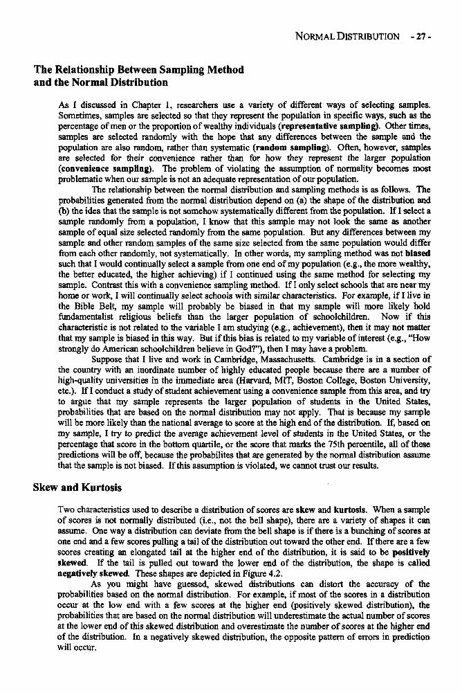
NORMAL DISTRIBUTION - 27 -
The Relationship Between Sampling Methodand the Normal Distribution
As I discussed in Chapter 1, researchers use a variety of different ways of selecting samples.Sometimes, samples are selected so that they represent the population in specific ways, such as thepercentage of men or the proportion of wealthy individuals (representative sampling). Other times,samples are selected randomly with the hope that any differences between the sample and thepopulation are also random, rather than systematic (random sampling). Often, however, samplesare selected for their convenience rather than for how they represent the larger population(convenience sampling). The problem of violating the assumption of normality becomes mostproblematic when our sample is not an adequate representation of our population.
The relationship between the normal distribution and sampling methods is as follows. Theprobabilities generated from the normal distribution depend on (a) the shape of the distribution and(b) the idea that the sample is not somehow systematically different from the population. If I select asample randomly from a population, I know that this sample may not look the same as anothersample of equal size selected randomly from the same population. But any differences between mysample and other random samples of the same size selected from the same population would differfrom each other randomly, not systematically. In other words, my sampling method was not biasedsuch that I would continually select a sample from one end of my population (e.g., the more wealthy,the better educated, the higher achieving) if I continued using the same method for selecting mysample. Contrast this with a convenience sampling method. If I only select schools that are near myhome or work, I will continually select schools with similar characteristics. For example, if I live inthe Bible Belt, my sample will probably be biased in that my sample will more likely holdfundamentalist religious beliefs than the larger population of schoolchildren. Now if thischaracteristic is not related to the variable I am studying (e.g., achievement), then it may not matterthat my sample is biased in this way. But if this bias is related to my variable of interest (e.g., "Howstrongly do American schoolchildren believe in God?"), then I may have a problem.
Suppose that I live and work in Cambridge, Massachusetts. Cambridge is in a section ofthe country with an inordinate number of highly educated people because there are a number ofhigh-quality universities in the immediate area (Harvard, MIT, Boston College, Boston University,etc.). If I conduct a study of student achievement using a convenience sample from this area, and tryto argue that my sample represents the larger population of students in the United States,probabilities that are based on the normal distribution may not apply. That is because my samplewill be more likely than the national average to score at the high end of the distribution. If, based onmy sample, I try to predict the average achievement level of students in the United States, or thepercentage that score in the bottom quartile, or the score that marks the 75th percentile, all of thesepredictions will be off, because the probabilites that are generated by the normal distribution assumethat the sample is not biased. If this assumption is violated, we cannot trust our results.
Skew and Kurtosis
Two characteristics used to describe a distribution of scores are skew and kurtosis. When a sampleof scores is not normally distributed (i.e., not the bell shape), there are a variety of shapes it canassume. One way a distribution can deviate from the bell shape is if there is a bunching of scores atone end and a few scores pulling a tail of the distribution out toward the other end. If there are a fewscores creating an elongated tail at the higher end of the distribution, it is said to be positivelyskewed. If the tail is pulled out toward the lower end of the distribution, the shape is callednegatively skewed. These shapes are depicted in Figure 4.2.
As you might have guessed, skewed distributions can distort the accuracy of theprobabilities based on the normal distribution. For example, if most of the scores in a distributionoccur at the low end with a few scores at the higher end (positively skewed distribution), theprobabilities that are based on the normal distribution will underestimate the actual number of scoresat the lower end of this skewed distribution and overestimate the number of scores at the higher endof the distribution. In a negatively skewed distribution, the opposite pattern of errors in predictionwill occur.
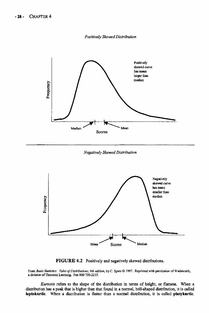
-28- CHAPTER 4
FIGURE 4.2 Positively and negatively skewed distributions.
From Basic Statistics: Tales of Distributions, 6th edition, by C. Spatz © 1997. Reprinted with permission of Wadsworth,a division of Thomson Learning. Fax 800 730-2215.
Kurtosis refers to the shape of the distribution in terms of height, or flatness. When adistribution has a peak that is higher than that found in a normal, bell-shaped distribution, it is calledleptokurtic. When a distribution is flatter than a normal distribution, it is called platykurtic.
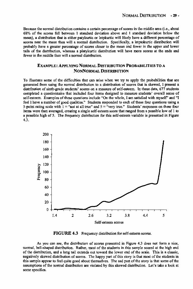
NORMAL DISTRIBUTION - 29 -
Because the normal distribution contains a certain percentage of scores in the middle area (i.e., about68% of the scores fall between 1 standard deviation above and 1 standard deviation below themean), a distribution that is either patykurtic or letpkurtic will likely have a different percentage ofscores near the mean than will a normal distribution. Specifically, a letptokurtic distribution willprobably have a greater percentage of scores closer to the mean and fewer in the upper and lowertails of the distribution, whereas a platykurtic distribution will have more scores at the ends andfewer in the middle than will a normal distribution.
EXAMPLE: APPLYING NORMAL DISTRIBUTION PROBABILITIES TO ANONNORMAL DISTRIBUTION
To illustrate some of the difficulties that can arise when we try to apply the probabilities that aregenerated from using the normal distribution to a distribution of scores that is skewed, I present adistribution of sixth-grade students' scores on a measure of self-esteem. In these data, 677 studentscompleted a questionnaire that included four items designed to measure students' overall sense ofself-esteem. Examples of these questions include "On the whole, I am satisfied with myself and "Ifeel I have a number of good qualities." Students responded to each of these four questions using a5-point rating scale with 1 = "not at all true" and 5 = "very true." Students' responses on these fouritems were then averaged, creating a single self-esteem score that ranged from a possible low of 1 toa possible high of 5. The frequency distribution for this self-esteem variable is presented in Figure4.3.
FIGURE 4.3 Frequency distribution for self-esteem scores.
As you can see, the distribution of scores presented in Figure 4.3 does not form a nice,normal, bell-shaped distribution. Rather, most of the students in this sample scored at the high endof the distribution, and a long tail extends out toward the lower end of the scale. This is a classic,negatively skewed distribution of scores. The happy part of this story is that most of the students inthis sample appear to feel quite good about themselves. The sad part of the story is that some of theassumptions of the normal distribution are violated by this skewed distribution. Let's take a look atsome specifics.
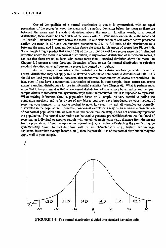
-30- CHAPTER 4
One of the qualities of a normal distribution is that it is symmetrical, with an equalpercentage of the scores between the mean and 1 standard deviation below the mean as there arebetween the mean and 1 standard deviation above the mean. In other words, in a normaldistribution, there should be about 34% of the scores within 1 standard deviation above the mean and34% within 1 standard deviation below the mean. In our distribution of self-esteem scores presentedearlier, the mean is 4.28 and the standard deviation is .72. A full 50% of the distribution fallsbetween the mean and 1 standard deviation above the mean in this group of scores (see Figure 4.4).So, although I might predict that about 16% of my distribution will have scores more than 1 standarddeviation above the mean in a normal distribution, in my skewed distribution of self-esteem scores, Ican see that there are no students with scores more than 1 standard deviation above the mean. InChapter 5, I present a more thorough discussion of how to use the normal distribution to calculatestandard deviation units and percentile scores in a normal distribution.
As this example demonstrates, the probabilities that statisticians have generated using thenormal distribution may not apply well to skewed or otherwise nonnormal distributions of data. Thisshould not lead you to believe, however, that nonnormal distributions of scores are worthless. Infact, even if you have a nonnormal distribution of scores in your sample, these scores can createnormal sampling distributions for use in inferential statistics (see Chapter 6). What is perhaps mostimportant to keep in mind is that a nonnormal distribution of scores may be an indication that yoursample differs in important and systematic ways from the population that it is supposed to represent.When making inferences about a population based on a sample, be very careful to define thepopulation precisely and to be aware of any biases you may have introduced by your method ofselecting your sample. It is also important to note, however, that not all variables are normallydistributed in the population. Therefore, nonnormal sample data may be an accurate representationof nonnormal population data, as well as an indication that the sample does not accurately representthe population. The normal distribution can be used to generate probabilities about the likelihood ofselecting an individual or another sample with certain characteristics (e.g., distance from the mean)from a population. If your sample is not normal and your method of selecting the sample may besystematically biased to include those with certain characteristics (e.g., higher than averageachievers, lower than average income, etc.), then the probabilities of the normal distribution may notapply well to your sample.
FIGURE 4.4 The normal distribution divided into standard deviation units.
NORMAL DISTRIBUTION - 31 -
WRAPPING UP AND LOOKING FORWARD
The theoretical normal distribution is a critical element of statistics primarily because many of theprobabilities that are used in inferential statistics are based on the assumption of normaldistributions. As you will see in coming chapters, statisticians use these probabilities to determinethe probability of getting certain statistics and to make inferences about the population based on thesample. Even if the data in a sample are not normally distributed, it is possible that the data in thepopulation from which the sample was selected may be normally distributed. In Chapter 5, Idescribe how the normal distribution, through the use of z scores and standardization, is used todetermine the probability of obtaining an individual score from a sample that is a certain distanceaway from the sample mean. You will also learn about other fun statistics like percentile scores inChapter 5.
GLOSSARY OF TERMS FOR CHAPTER 4
Asymptotic: When the ends, or "tails," of a distribution never intersect with the X axis; they extendindefinitely.
Bell curve: The common term for the normal distribution. It is called the bell curve because of itsbell-like shape.
Biased: When a sample is not selected randomly, it may be a biased sample. A sample is biasedwhen the members are selected in a way that systematically overrepresents some segmentof the population and underrepresents other segments.
Convenience sampling: When a sample is selected because it is convenient rather than random.Descriptive statistics: Statistics that describe the characteristics of a given sample or population.
These statistics are only meant to describe the characteristics of those from whom data werecollected.
Inferential statistics: Statistics generated from sample data that are used to make inferences aboutthe characteristics of the population the sample is alleged to represent.
Kurtosis: The shape of a distribution of scores in terms of its flatness or peakedness.Leptokurtic: A term regarding the shape of a distribution. A leptokurtic distribution is one with a
higher peak and thinner tails.Negatively skewed: When a tail of a distribution of scores extends toward the lower end of the
distribution.Normal distribution: A bell-shaped distribution of scores that has the mean, median, and mode in
the middle of the distribution and is symmetrical and asymptotic.Null Hypohesis: A hypothesis that there is no effect.Platykurtic: A term regarding the shape of a distribution. A platykurtic distribution is one with a
lower peak and thicker tails.Population: The group from which data are collected or a sample is selected. The population
encompasses the entire group for which the data are alleged to apply.Positively skewed: When a tail of a distribution of scores extends toward the upper end of the
distribution.Probability: The likelihood of an event occurring.Random sampling: A method of selecting a sample in which every member of the population has
an equal chance of being selected.Representative sampling: A method of selecting a sample in which members are purposely
selected to create a sample that represents the population on some characteristics) ofinterest (e.g., when a sample is selected to have the same percentages of various ethnicgroups as the larger population).
Sample: An individual or group, selected from a population, from whom data are collected.Skew: The degree to which a distribution of scores deviates from normal in terms of asymmetrical
extension of the tails.

-32- CHAPTER 4
Symmetrical: When a distribution has the same shape on either side of the median.Theoretical distribution: A distribution based on statistical probabilities rather than empirical data.Unimodal: A distribution that has a single mode.
CHAPTER 5
STANDARDIZATION AND z SCORES
If you know the mean and standard deviation of a distribution of scores, you have enoughinformation to develop a picture of the distribution. Sometimes researchers are interested indescribing individual scores within a distribution. Using the mean and the standard deviation,researchers are able to generate a standard score, also called a z score, to help them understandwhere an individual score falls in relation to other scores in the distribution. Through a process ofstandardization, researchers are also better able to compare individual scores in the distributions oftwo separate variables. Standardization is simply a process of converting each score in a distributionto a z score. A z score is a number that indicates how far above or below the mean a given score inthe distribution is in standard deviation units. So standardization is simply the process of convertingindividual raw scores in the distribution into standard deviation units.
Suppose that you are a college student taking final exams. In your biology class, you takeyour final exam and get a score of 65 out of a possible 100. In your statistics final, you get a scoreof 42 out of 200. On which exam did you get a "better" score? The answer to this question may bemore complicated than it appears. First, we must determine what we mean by "better." If bettermeans percentage of correct answers on the exam, clearly you did better on the biology exam. But ifyour statistics exam was much more difficult than your biology exam, is it fair to judge yourperformance solely on the basis of percentage of correct responses? A more fair alternative may beto see how well you did compared to other students in your classes. To make such a comparison, weneed to know the mean and standard deviation of each distribution. With these statistics, we cangenerate z scores.
Suppose the mean on the biology exam was 60 with a standard deviation of 10. That meansyou scored 5 points above the mean, which is half of a standard deviation above the mean (higherthan the average for the class). Suppose further that the average on the statistics test was 37 with astandard deviation of 5. Again, you scored 5 points above the mean, but this represents a fullstandard deviation over the average. Using these statistics, on which test would you say youperformed better? To fully understand the answer to this question, let's examine standardization andz scores in more depth.
STANDARDIZATION AND z SCORES IN DEPTH
As you can see in the previous example, it is often difficult to compare two scores on two variableswhen the variables are measured using different scales. The biology test in the example wasmeasured on a scale from 1 to 100, whereas the statistics exam used a scale from 1 to 200. Whenvariables have such different scales of measurement, it is almost meaningless to compare the rawscores (i.e., 65 and 42 on these exams). Instead, we need some way to put these two exams on thesame scale, or to standardize them. One of the most common methods of standardization used instatistics is to convert raw scores into standard deviation units, or z scores. The formula for doingthis is very simple and is presented in Table 5.1.
As you can see from the formulas in Table 5.1, to standardize a score (i.e., to create a zscore), you simply subtract the mean from an individual raw score and divide this by the standarddeviation. So if the raw score is above the mean, the z score will be positive, whereas a raw scorebelow the mean will produce a negative z score. When an entire distribution of scores isstandardized, the average (i.e., mean) z score for the standardized distribution will always be 0, andthe standard deviation of this distribution will always be 1.0.
-33-
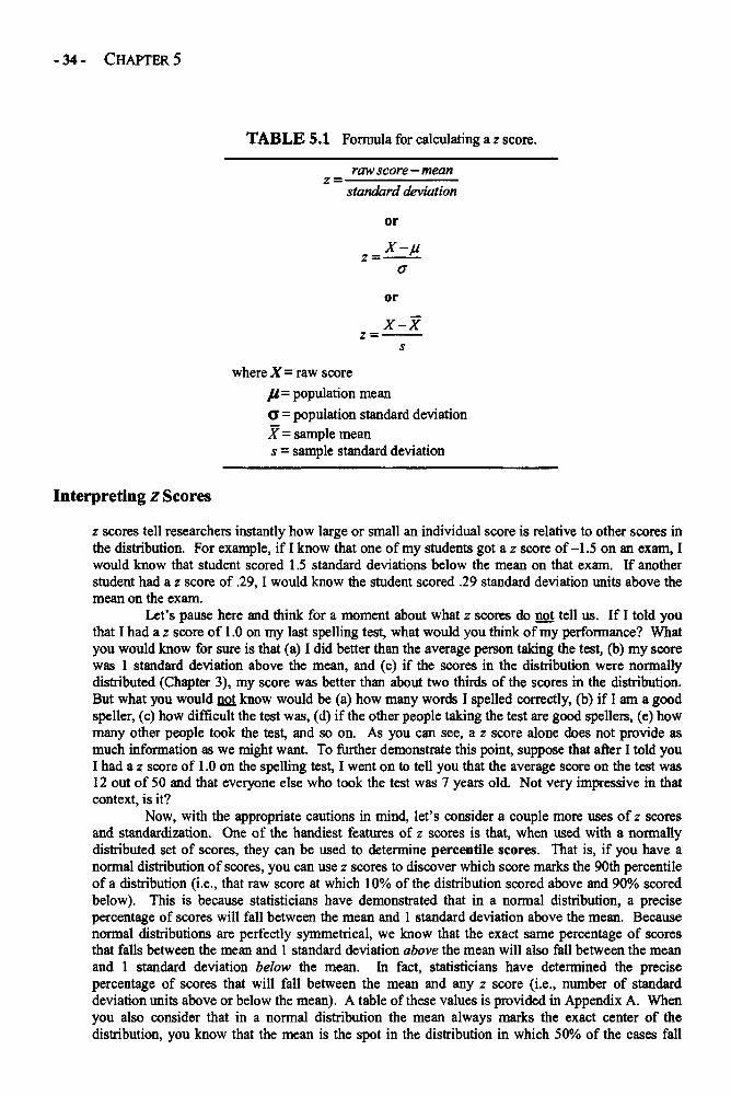
- 34 - CHAPTER 5
TABLE 5.1 Formula for calculating a z score.
raw score - mean
standard deviation
or
or
where X = raw score
u = population mean
o = population standard deviationX = sample means - sample standard deviation
Interpreting z Scores
z scores tell researchers instantly how large or small an individual score is relative to other scores inthe distribution. For example, if I know that one of my students got a z score of -1.5 on an exam, Iwould know that student scored 1.5 standard deviations below the mean on that exam. If anotherstudent had a z score of .29, I would know the student scored .29 standard deviation units above themean on the exam.
Let's pause here and think for a moment about what z scores do not tell us. If I told youthat I had a z score of 1.0 on my last spelling test, what would you think of my performance? Whatyou would know for sure is that (a) I did better than the average person taking the test, (b) my scorewas 1 standard deviation above the mean, and (c) if the scores in the distribution were normallydistributed (Chapter 3), my score was better than about two thirds of the scores in the distribution.But what you would not know would be (a) how many words I spelled correctly, (b) if I am a goodspeller, (c) how difficult the test was, (d) if the other people taking the test are good spellers, (e) howmany other people took the test, and so on. As you can see, a z score alone does not provide asmuch information as we might want. To further demonstrate this point, suppose that after I told youI had a z score of 1.0 on the spelling test, I went on to tell you that the average score on the test was12 out of 50 and that everyone else who took the test was 7 years old. Not very impressive in thatcontext, is it?
Now, with the appropriate cautions in mind, let's consider a couple more uses of z scoresand standardization. One of the handiest features of z scores is that, when used with a normallydistributed set of scores, they can be used to determine percentile scores. That is, if you have anormal distribution of scores, you can use z scores to discover which score marks the 90th percentileof a distribution (i.e., that raw score at which 10% of the distribution scored above and 90% scoredbelow). This is because statisticians have demonstrated that in a normal distribution, a precisepercentage of scores will fall between the mean and 1 standard deviation above the mean. Becausenormal distributions are perfectly symmetrical, we know that the exact same percentage of scoresthat falls between the mean and 1 standard deviation above the mean will also fall between the meanand 1 standard deviation below the mean. In fact, statisticians have determined the precisepercentage of scores that will fall between the mean and any z score (i.e., number of standarddeviation units above or below the mean). A table of these values is provided in Appendix A. Whenyou also consider that in a normal distribution the mean always marks the exact center of thedistribution, you know that the mean is the spot in the distribution in which 50% of the cases fall
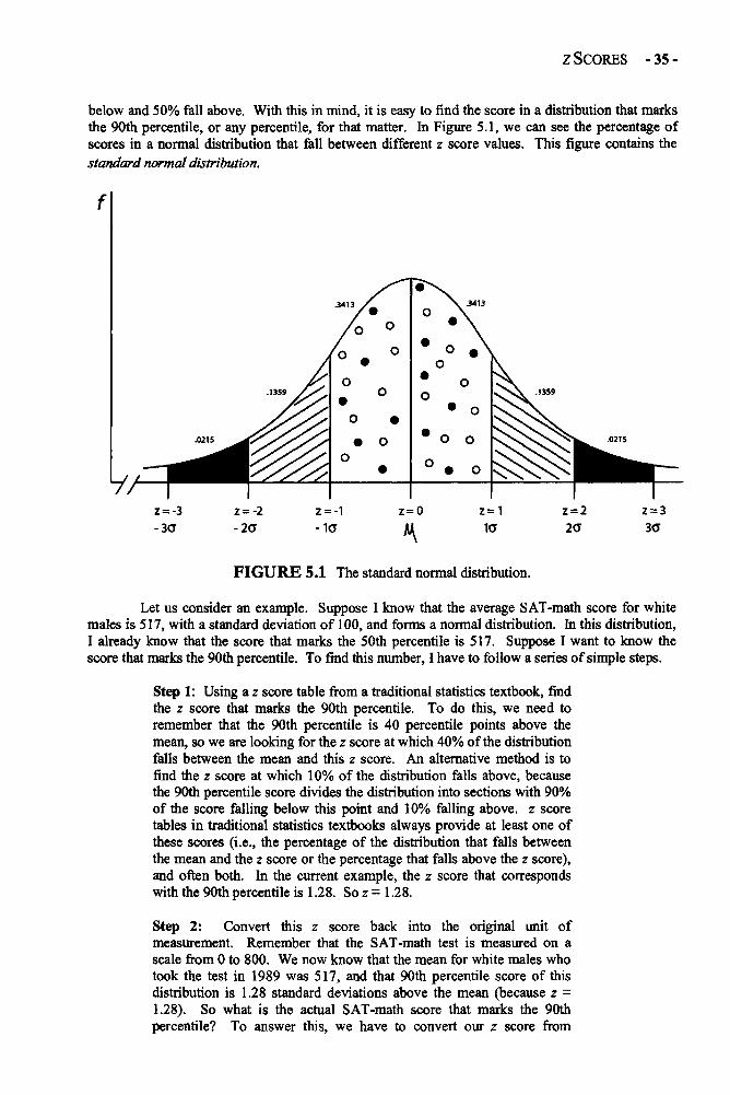
zSCORES -35-
below and 50% fall above. With this in mind, it is easy to find the score in a distribution that marksthe 90th percentile, or any percentile, for that matter. In Figure 5.1, we can see the percentage ofscores in a normal distribution that fall between different z score values. This figure contains thestandard normal distribution.
FIGURE 5.1 The standard normal distribution.
Let us consider an example. Suppose I know that the average SAT-math score for whitemales is 517, with a standard deviation of 100, and forms a normal distribution. In this distribution,I already know that the score that marks the 50th percentile is 517. Suppose I want to know thescore that marks the 90th percentile. To find this number, I have to follow a series of simple steps.
Step 1: Using a z score table from a traditional statistics textbook, findthe z score that marks the 90th percentile. To do this, we need toremember that the 90th percentile is 40 percentile points above themean, so we are looking for the z score at which 40% of the distributionfalls between the mean and this z score. An alternative method is tofind the z score at which 10% of the distribution falls above, becausethe 90th percentile score divides the distribution into sections with 90%of the score falling below this point and 10% falling above, z scoretables in traditional statistics textbooks always provide at least one ofthese scores (i.e., the percentage of the distribution that falls betweenthe mean and the z score or the percentage that falls above the z score),and often both. In the current example, the z score that correspondswith the 90th percentile is 1.28. So z = 1.28.
Step 2: Convert this z score back into the original unit ofmeasurement. Remember that the SAT-math test is measured on ascale from 0 to 800. We now know that the mean for white males whotook the test in 1989 was 517, and that 90th percentile score of thisdistribution is 1.28 standard deviations above the mean (because z =1.28). So what is the actual SAT-math score that marks the 90thpercentile? To answer this, we have to convert our z score from
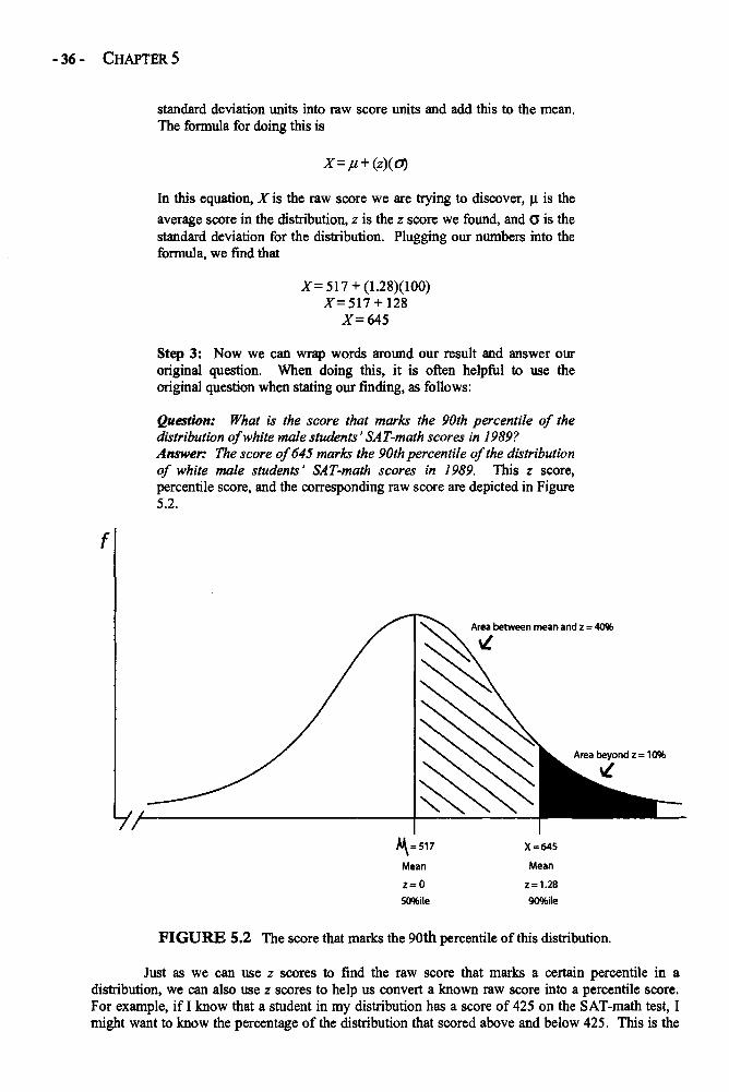
- 36 - CHAPTER 5
standard deviation units into raw score units and add this to the mean.The formula for doing this is
In this equation, X is the raw score we are trying to discover, u is the
average score in the distribution, z is the z score we found, and o is thestandard deviation for the distribution. Plugging our numbers into theformula, we find that
Z=517 + (1.28)(100)X=517+128
X=645
Step 3: Now we can wrap words around our result and answer ouroriginal question. When doing this, it is often helpful to use theoriginal question when stating our finding, as follows:
Question: What is the score that marks the 90th percentile of thedistribution of white male students' SAT-math scores in 1989?Answer: The score of 645 marks the 90th percentile of the distributionof white male students' SAT-math scores in 1989. This z score,percentile score, and the corresponding raw score are depicted in Figure5.2.
FIGURE 5.2 The score that marks the 90th percentile of this distribution.
Just as we can use z scores to find the raw score that marks a certain percentile in adistribution, we can also use z scores to help us convert a known raw score into a percentile score.For example, if I know that a student in my distribution has a score of 425 on the SAT-math test, Imight want to know the percentage of the distribution that scored above and below 425. This is the
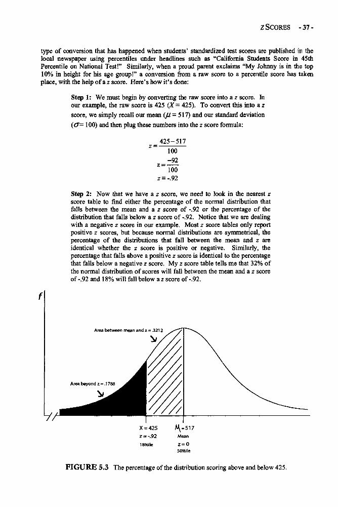
z SCORES -37-
type of conversion that has happened when students' standardized test scores are published in thelocal newspaper using percentiles under headlines such as "California Students Score in 45thPercentile on National Test!" Similarly, when a proud parent exclaims "My Johnny is in the top10% in height for his age group!" a conversion from a raw score to a percentile score has takenplace, with the help of a z score. Here's how it's done:
Step 1: We must begin by converting the raw score into a z score. Inour example, the raw score is 425 (X = 425). To convert this into a z
score, we simply recall our mean (u = 517) and our standard deviation
(o= 100) and then plug these numbers into the z score formula:
Step 2: Now that we have a z score, we need to look in the nearest zscore table to find either the percentage of the normal distribution thatfalls between the mean and a z score of -.92 or the percentage of thedistribution that falls below a z score of -.92. Notice that we are dealingwith a negative z score in our example. Most z score tables only reportpositive z scores, but because normal distributions are symmetrical, thepercentage of the distributions that fall between the mean and z areidentical whether the z score is positive or negative. Similarly, thepercentage that falls above a positive z score is identical to the percentagethat falls below a negative z score. My z score table tells me that 32% ofthe normal distribution of scores will fall between the mean and a z scoreof-.92 and 18% will fall below a z score of-.92.
FIGURE 5.3 The percentage of the distribution scoring above and below 425.
- 38 - CHAPTER 5
Step 3: To wrap words around this result, I must begin with therecollection that in my example, a z score of -.88 corresponds with araw score of 425 on the SAT-math test among the white males whotook the test in 1989. So, I would say, "A score of 425 on the SAT-math test marks the 19th percentile of the distribution of test scoresamong white males in 1989." (See Figure 5.3 for a graph of thispercentile score.)
z scores used with a normal distribution can also be used to figure out the proportion ofscores that fall between two raw scores. For example, suppose that you got a score of 417 on theSAT-math test and your friend got a score of 567. "Wow!" your friend says. "I blew you away!There must be about 50% of the population that scored between you and me on this test." Your egobruised, you decide to see if your friend is right in his assessment. Here's what you need to do.
Step 1: First, convert each raw score into z scores. Recall the mean (u
= 517) and standard deviation (o= 100) and then plug these numbersinto the z score formula:
Your z score
Your friend's z score
Step 2: Now that we have the z scores, we need to look in the nearest zscore table to find either the percentage of the normal distribution thatfalls between the mean and a z score of-1.00 and the percentage of thedistribution that falls between the mean and a z score of .50. Notice thatwe are dealing with one negative and one positive z score in our example.Our z score table tells me that 34.13% of the normal distribution of scoreswill fall between the mean and a z score of -1.00 and 19.15% will fallbetween the mean and a z score of .50. To determine the total proportionof scores that fall between these two z scores, we need to add the twoproportions together: .3413 + .1915 = .5328.
Step 3: Admit defeat in a bitter and defensive way. "Ha ha," you sayto your friend. "It is not 50% of the population that scored betweenyou and me on the SAT-math test. It was 53.28%!" (See Figure 5.4.)
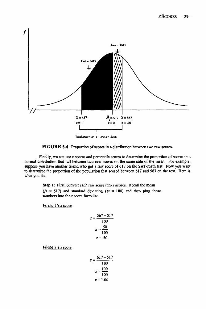
z SCORES -39-
FIGURE 5.4 Proportion of scores in a distribution between two raw scores.
Finally, we can use z scores and percentile scores to determine the proportion of scores in anormal distribution that fall between two raw scores on the same side of the mean. For example,suppose you have another friend who got a raw score of 617 on the SAT-math test. Now you wantto determine the proportion of the population that scored between 617 and 567 on the test. Here iswhat you do.
Step 1: First, convert each raw score into z scores. Recall the mean(u = 517) and standard deviation (o = 100) and then plug thesenumbers into the z score formula:
Friend 1's z score
Friend 2's z score
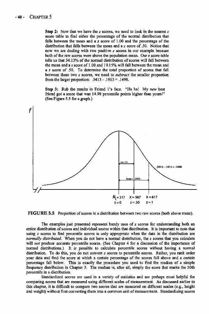
- 40 - CHAPTER 5
Step 2: Now that we have the z scores, we need to look in the nearest zscore table to find either the percentage of the normal distribution thatfalls between the mean and a z score of 1.00 and the percentage of thedistribution that falls between the mean and a z score of .50. Notice thatnow we are dealing with two positive z scores in our example becauseboth of the raw scores were above the population mean. Our z score tabletells us that 34.13% of the normal distribution of scores will fall betweenthe mean and a z score of 1.00 and 19.15% will fall between the mean anda z score of .50. To determine the total proportion of scores that fallbetween these two z scores, we need to subtract the smaller proportionfrom the larger proportion: .3413 - .1915 = .1498.
Step 3: Rub the results in Friend 1's face. "Ha ha! My new bestfriend got a score that was 14.98 percentile points higher than yours!"(See Figure 5.5 for a graph.)
FIGURE 5.5 Proportion of scores in a distribution between two raw scores (both above mean).
The examples just presented represent handy uses of z scores for understanding both anentire distribution of scores and individual scores within that distribution. It is important to note thatusing z scores to find percentile scores is only appropriate when the data in the distribution arenormally distributed. When you do not have a normal distribution, the z scores that you calculatewill not produce accurate percentile scores. (See Chapter 4 for a discussion of the importance ofnormal distributions.) It is possible to calculate percentile scores without having a normaldistribution. To do this, you do not convert z scores to percentile scores. Rather, you rank orderyour data and find the score at which a certain percentage of the scores fall above and a certainpercentage fall below. This is exactly the procedure you used to find the median of a simplefrequency distribution in Chapter 3. The median is, after all, simply the score that marks the 50thpercentile in a distribution.
Standardized scores are used in a variety of statistics and are perhaps most helpful forcomparing scores that are measured using different scales of measurement. As discussed earlier inthis chapter, it is difficult to compare two scores that are measured on different scales (e.g., heightand weight) without first converting them into a common unit of measurement. Standardizing scores
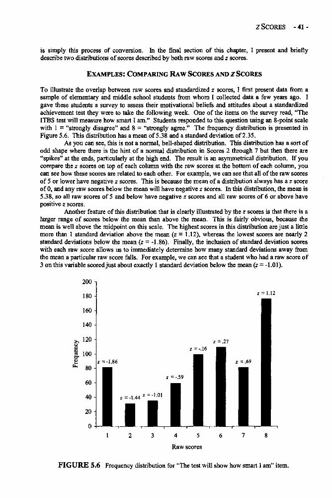
z SCORES -41-
is simply this process of conversion. In the final section of this chapter, I present and brieflydescribe two distributions of scores described by both raw scores and z scores.
EXAMPLES: COMPARING RAW SCORES AND z SCORES
To illustrate the overlap between raw scores and standardized z scores, I first present data from asample of elementary and middle school students from whom I collected data a few years ago. Igave these students a survey to assess their motivational beliefs and attitudes about a standardizedachievement test they were to take the following week. One of the items on the survey read, "TheITBS test will measure how smart I am." Students responded to this question using an 8-point scalewith 1 = "strongly disagree" and 8 = "strongly agree." The frequency distribution is presented inFigure 5.6. This distribution has a mean of 5.38 and a standard deviation of 2.35.
As you can see, this is not a normal, bell-shaped distribution. This distribution has a sort ofodd shape where there is the hint of a normal distribution in Scores 2 through 7 but then there are"spikes" at the ends, particularly at the high end. The result is an asymmetrical distribution. If youcompare the z scores on top of each column with the raw scores at the bottom of each column, youcan see how these scores are related to each other. For example, we can see that all of the raw scoresof 5 or lower have negative z scores. This is because the mean of a distribution always has a z scoreof 0, and any raw scores below the mean will have negative z scores. In this distribution, the mean is5.38, so all raw scores of 5 and below have negative z scores and all raw scores of 6 or above havepositive z scores.
Another feature of this distribution that is clearly illustrated by the z scores is that there is alarger range of scores below the mean than above the mean. This is fairly obvious, because themean is well above the midpoint on this scale. The highest scores in this distribution are just a littlemore than 1 standard deviation above the mean (z = 1.12), whereas the lowest scores are nearly 2standard deviations below the mean (z = -1.86). Finally, the inclusion of standard deviation scoreswith each raw score allows us to immediately determine how many standard deviations away fromthe mean a particular raw score falls. For example, we can see that a student who had a raw score of3 on this variable scored just about exactly 1 standard deviation below the mean (z = -1.01).
FIGURE 5.6 Frequency distribution for "The test will show how smart I am" item.
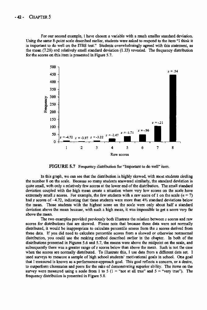
- 42 - CHAPTER 5
For our second example, I have chosen a variable with a much smaller standard deviation.Using the same 8-point scale described earlier, students were asked to respond to the item "I think itis important to do well on the UBS test." Students overwhelmingly agreed with this statement, asthe mean (7.28) and relatively small standard deviation (1.33) revealed. The frequency distributionfor the scores on this item is presented in Figure 5.7.
FIGURE 5.7 Frequency distribution for "Important to do well" item.
In this graph, we can see that the distribution is highly skewed, with most students circlingthe number 8 on the scale. Because so many students answered similarly, the standard deviation isquite small, with only a relatively few scores at the lower end of the distribution. The small standarddeviation coupled with the high mean create a situation where very low scores on the scale haveextremely small z scores. For example, the few students with a raw score of 1 on the scale (n = 7)had z scores of -4.72, indicating that these students were more than 4% standard deviations belowthe mean. Those students with the highest score on the scale were only about half a standarddeviation above the mean because, with such a high mean, it was impossible to get a score very farabove the mean.
The two examples provided previously both illustrate the relation between z scores and rawscores for distributions that are skewed. Please note that because these data were not normallydistributed, it would be inappropriate to calculate percentile scores from the z scores derived fromthese data. If you did need to calculate percentile scores from a skewed or otherwise nonnormaldistribution, you could use the ranking method described earlier in the chapter. In both of thedistributions presented in Figures 5.6 and 5.7, the means were above the midpoint on the scale, andsubsequently there was a greater range of z scores below than above the mean. Such is not the casewhen the scores are normally distributed. To illustrate this, I use data from a different data set. Iused surveys to measure a sample of high school students' motivational goals in school. One goalthat I measured is known as a performance-approach goal. This goal reflects a concern, or a desire,to outperform classmates and peers for the sake of demonstrating superior ability. The items on thesurvey were measured using a scale from 1 to 5 (1 = "not at all true" and 5 = "very true"). Thefrequency distribution is presented in Figure 5.8.
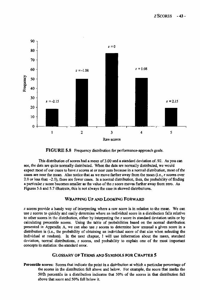
z SCORES -43-
FIGURE 5.8 Frequency distribution for performance-approach goals.
This distribution of scores had a mean of 3.00 and a standard deviation of .92. As you cansee, the data are quite normally distributed. When the data are normally distributed, we wouldexpect most of our cases to have z scores at or near zero because in a normal distribution, most of thecases are near the mean. Also notice that as we move farther away from the mean (i.e., z scores over2.0 or less than -2.0), there are fewer cases. In a normal distribution, then, the probability of findinga particular z score becomes smaller as the value of the z score moves further away from zero. AsFigures 5.6 and 5.7 illustrate, this is not always the case in skewed distributions.
WRAPPING UP AND LOOKING FORWARD
z scores provide a handy way of interpreting where a raw score is in relation to the mean. We canuse z scores to quickly and easily determine where an individual score in a distribution falls relativeto other scores in the distribution, either by interpreting the z score in standard deviation units or bycalculating percentile scores. Using the table of probabilities based on the normal distributionpresented in Appendix A, we can also use z scores to determine how unusual a given score in adistribution is (i.e., the probability of obtaining an individual score of that size when selecting theindividual at random). In the next chapter, I will use information about the mean, standarddeviation, normal distributions, z scores, and probability to explain one of the most importantconcepts in statistics: the standard error.
GLOSSARY OF TERMS AND SYMBOLS FOR CHAPTER 5
Percentile scores: Scores that indicate the point in a distribution at which a particular percentage ofthe scores in the distribution fall above and below. For example, the score that marks the50th percentile in a distribution indicates that 50% of the scores in that distribution fallabove that score and 50% fall below it.

- 44 - CHAPTER 5
Raw scores: These are the individual observed scores on measured variables.Standard score: A raw score that has been converted to a z score by subtracting it from the mean
and dividing by the standard deviation of the distribution. It is an individual scoreexpressed as a deviation from the mean in standard deviation units.
Standardization: The process of converting a raw score into a standard score.z score: Another term for a standard score.
z A standard score.X A raw score.
u A population mean.
a A population standard deviation.
CHAPTER 6
STANDARD ERRORS
The concept of standard error is one that many students of statistics find confusing when they firstencounter it. In all honesty, there are many students, and many researchers, who never fully graspthe concept. I am convinced that many people have problems with understanding standard errorsbecause they require a bit of a leap into the abstract and because, with the advent of computerprograms, it is possible to lead a long and productive research life without having to think about oranalyze a standard error for years at a time. Therefore, many researchers choose to gloss over thisabstract concept. This is a mistake. I hold this opinion because, as a teacher of statistics, I havelearned that when one is able to truly understand the concept of standard error, many of our mostbeloved inferential statistics (t tests, ANOVA, regression coefficients, correlations) become easy tounderstand. So let me offer this piece of advice: Keep trying to understand the contents of thischapter, and other information you get about standard errors, even if you find it confusing the first orsecond time you read it. With a little effort and patience, you can understand standard errors andmany of the statistics that rely on them.
What Is a Standard Error?
There are two answers to this question. First, there is the technical answer, which is the definition ofa standard error. A standard error is, in effect, the standard deviation of the sampling distributionof some statistic (e.g., the mean, the difference between two means, the correlation coefficient, etc.).I realize that this makes no sense until you know what a sampling distribution is, and I explain this inthe next section of this chapter. For now, I recommend that you repeat the definition to yourself 10times: "The standard error is, in effect, the standard deviation of the sampling distribution of somestatistic."
The second answer is that the standard error is the denominator in the formulas used tocalculate many inferential statistics. In the following chapters, you will see the standard error as thedenominator in many formulas. This is because the standard error is the measure of how muchrandom variation we would expect from samples of equal size drawn from the same population.Again, look at the preceding sentence, think about it, and rest assured that it is explained in moredetail in the next few pages.
STANDARD ERRORS IN DEPTH
The Conceptual Description of the Standard Error of the Mean
To begin this more detailed discussion of standard errors, I introduce the esoteric component of theconcept. This is the section that you may need to read several times to let sink in. Although thereare standard errors for all statistics, we will focus on the standard error of the mean.
When we think of a distribution of scores, we think of a certain number of scores that areplotted in some sort of frequency graph to form a distribution (see Chapters 2 and 4). In thesedistributions, each case has a score that is part of the distribution. Just as these simple frequencydistributions are plotted, or graphed, we can also plot distributions of sample means. Imagine thatwe want to find the average shoe size of adult women in the United States. In this study, thepopulation we are interested in is all adult American women. But it would be expensive and tediousto measure the shoe size of all adult American women. So we select a sample of 100 women, at
- 45 -
-46- CHAPTER 6
random, from our population. At this point, it is very important to realize that our sample of 100women may or may not look like the typical Amemrican woman (in terms of shoe size). When weselect a sample at random, it is possible to get a sample that represents an extreme end of thepopulation (e.g., a sample with an unusually large average shoe size). If we were to throw our firstsample of women back into the general population and chose another random sample of the samesize (i.e., 100), it is possible that this second sample may have an average shoe size that is quitedifferent from our first sample.
Once you realize that different random samples of equal size can produce different meanscores on some variable (e.g., different average shoe sizes), the next step in this conceptual puzzle iseasy: If we were to take 1,000 different random samples of women, each of 100, and compute theaverage shoe size of each sample, these 1,000 sample means would form their own distribution.This distribution would be called the sampling distribution of the mean.
To illustrate this concept, let's consider an example with a small population (N = 5).Suppose my population consists of five college students enrolled in a seminar on statistics. Becauseit is a small seminar, these five students represent the entire population of this seminar. Thesestudents each took the final exam that was scored on a scale from 1 to 10, with lower scoresindicating poorer performance on the exam. The scores for each student are presented in Table 6.1,arranged in descending order according to how well they did on the exam.
TABLE 6.1 Population of students' scores on final exam.
Students
Student 1
Student 2
Student 3
Student 4
Student 5
Score on Final Exam
3
6
6
7
9
If I were to select a random sample of two students from this population (n = 2), I might getstudent 2 and student 5. This sample would have a mean of 7.5 because [(6 + 9) + 2 = 7.5]. If Iwere to put those two students back into the population and randomly select another sample of 2, 1might get Student 4 and Student 5. This sample would have a mean of 8 because [(7 + 9) + 2 = 8]. Iput those students back into the population and randomly select another sample of 2, such asStudents 1 and 3. This sample would have a mean of 4.5. As you can see, just by virtue of thoseincluded in each random sample I select from my population, I get different sample means. Now if Iwere to repeat this process of randomly selecting samples of two students from my population,calculating their mean, and returning the members of the sample to the population (called samplingwith replacement), eventually I would get a distribution of sample means that would look somethinglike the distribution presented in Figure 6.1. As you can see, these means form a distribution. Thisexample illustrates how random samples of a given size selected from a population will produce adistribution of sample means, eventually forming a sampling distribution of the mean.
Just as the other distributions we have discussed have a mean and a standard deviation, thissampling distribution of the mean also has these characteristics. To distinguish a samplingdistribution from a simple frequency distribution, the mean and standard deviation of the samplingdistribution of the mean have special names. The mean of the sampling distribution of the mean iscalled the expected value of the mean. It is called the expected value because the mean of thesampling distribution of the means is the same as the population mean. When we select a samplefrom the population, our best guess is that the mean for the sample will be the same as the mean forthe population, so our expected mean will be the population mean. The standard deviation of thesampling distribution of the mean is called the standard error. So the standard error is simply thestandard deviation of the sampling distribution.
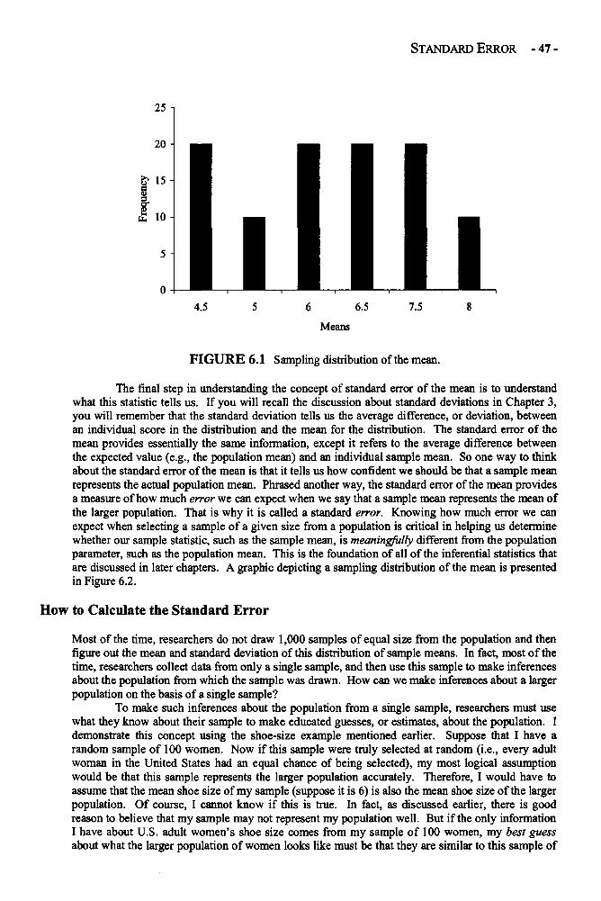
STANDARD ERROR - 47 -
FIGURE 6.1 Sampling distribution of the mean.
The final step in understanding the concept of standard error of the mean is to understandwhat this statistic tells us. If you will recall the discussion about standard deviations in Chapter 3,you will remember mat the standard deviation tells us the average difference, or deviation, betweenan individual score in the distribution and the mean for the distribution. The standard error of themean provides essentially the same information, except it refers to the average difference betweenthe expected value (e.g., the population mean) and an individual sample mean. So one way to thinkabout the standard error of the mean is that it tells us how confident we should be that a sample meanrepresents the actual population mean. Phrased another way, the standard error of the mean providesa measure of how much error we can expect when we say that a sample mean represents the mean ofthe larger population. That is why it is called a standard error. Knowing how much error we canexpect when selecting a sample of a given size from a population is critical in helping us determinewhether our sample statistic, such as the sample mean, is meaningfully different from the populationparameter, such as the population mean. This is the foundation of all of the inferential statistics thatare discussed in later chapters. A graphic depicting a sampling distribution of the mean is presentedin Figure 6.2.
How to Calculate the Standard Error
Most of the time, researchers do not draw 1,000 samples of equal size from the population and thenfigure out the mean and standard deviation of this distribution of sample means. In fact, most of thetime, researchers collect data from only a single sample, and then use this sample to make inferencesabout the population from which the sample was drawn. How can we make inferences about a largerpopulation on the basis of a single sample?
To make such inferences about the population from a single sample, researchers must usewhat they know about their sample to make educated guesses, or estimates, about the population. Idemonstrate this concept using the shoe-size example mentioned earlier. Suppose that I have arandom sample of 100 women. Now if this sample were truly selected at random (i.e., every adultwoman in the United States had an equal chance of being selected), my most logical assumptionwould be that this sample represents the larger population accurately. Therefore, I would have toassume that the mean shoe size of my sample (suppose it is 6) is also the mean shoe size of the largerpopulation. Of course, I cannot know if this is true. In fact, as discussed earlier, there is goodreason to believe that my sample may not represent my population well. But if the only informationI have about U.S. adult women's shoe size conies from my sample of 100 women, my best guessabout what the larger population of women looks like must be that they are similar to this sample of
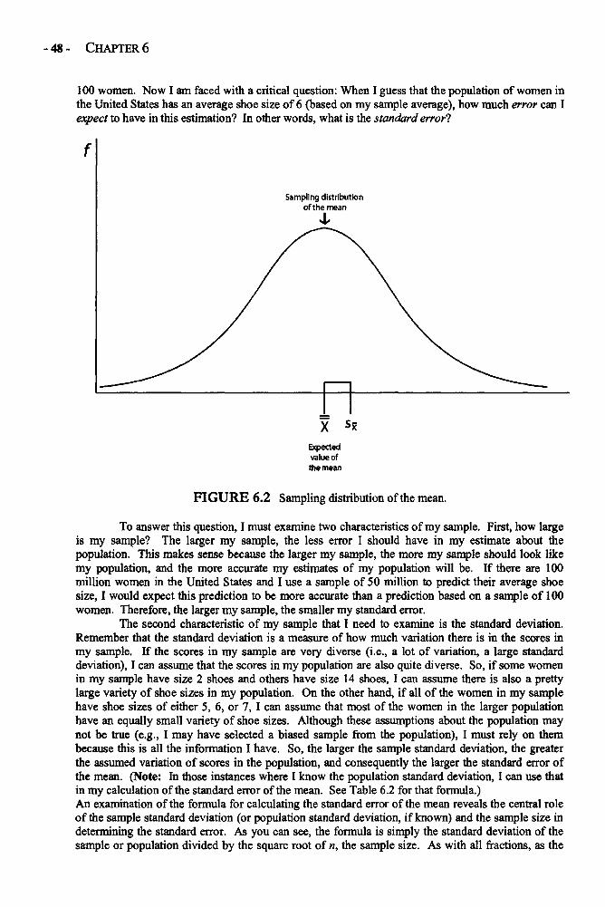
- 48 - CHAPTER 6
100 women. Now I am faced with a critical question: When I guess that the population of women inthe United States has an average shoe size of 6 (based on my sample average), how much error can Iexpect to have in this estimation? In other words, what is the standard error?
FIGURE 6.2 Sampling distribution of the mean.
To answer this question, I must examine two characteristics of my sample. First, how largeis my sample? The larger my sample, the less error I should have in my estimate about thepopulation. This makes sense because the larger my sample, the more my sample should look likemy population, and the more accurate my estimates of my population will be. If there are 100million women in the United States and I use a sample of 50 million to predict their average shoesize, I would expect this prediction to be more accurate than a prediction based on a sample of 100women. Therefore, the larger my sample, the smaller my standard error.
The second characteristic of my sample that I need to examine is the standard deviation.Remember that the standard deviation is a measure of how much variation there is in the scores inmy sample. If the scores in my sample are very diverse (i.e., a lot of variation, a large standarddeviation), I can assume that the scores in my population are also quite diverse. So, if some womenin my sample have size 2 shoes and others have size 14 shoes, I can assume there is also a prettylarge variety of shoe sizes in my population. On the other hand, if all of the women in my samplehave shoe sizes of either 5, 6, or 7, I can assume that most of the women in the larger populationhave an equally small variety of shoe sizes. Although these assumptions about the population maynot be true (e.g., I may have selected a biased sample from the population), I must rely on thembecause this is all the information I have. So, the larger the sample standard deviation, the greaterthe assumed variation of scores in the population, and consequently the larger the standard error ofthe mean. (Note: In those instances where I know the population standard deviation, I can use thatin my calculation of the standard error of the mean. See Table 6.2 for that formula.)An examination of the formula for calculating the standard error of the mean reveals the central roleof the sample standard deviation (or population standard deviation, if known) and the sample size indetermining the standard error. As you can see, the formula is simply the standard deviation of thesample or population divided by the square root of n, the sample size. As with all fractions, as the
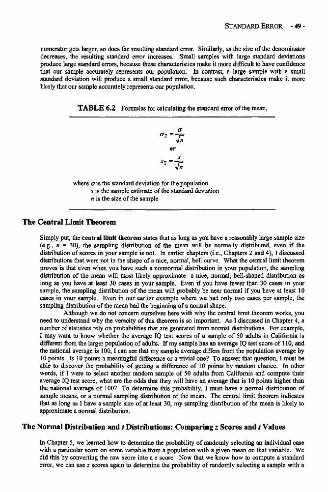
STANDARD ERROR - 49 -
numerator gets larger, so does the resulting standard error. Similarly, as the size of the denominatordecreases, the resulting standard error increases. Small samples with large standard deviationsproduce large standard errors, because these characteristics make it more difficult to have confidencethat our sample accurately represents our population. In contrast, a large sample with a smallstandard deviation will produce a small standard error, because such characteristics make it morelikely that our sample accurately represents our population.
TABLE 6.2 Formulas for calculating the standard error of the mean.
where a is the standard deviation for the populations is the sample estimate of the standard deviationn is the size of the sample
The Central Limit Theorem
Simply put, the central limit theorem states that as long as you have a reasonably large sample size(e.g., n = 30), the sampling distribution of the mean will be normally distributed, even if thedistribution of scores in your sample is not. In earlier chapters (i.e., Chapters 2 and 4), I discusseddistributions that were not in the shape of a nice, normal, bell curve. What the central limit theoremproves is that even when you have such a nonnormal distribution in your population, the samplingdistribution of the mean will most likely approximate a nice, normal, bell-shaped distribution aslong as you have at least 30 cases in your sample. Even if you have fewer than 30 cases in yoursample, the sampling distribution of the mean will probably be near normal if you have at least 10cases in your sample. Even in our earlier example where we had only two cases per sample, thesampling distribution of the mean had the beginning of a normal shape.
Although we do not concern ourselves here with why the central limit theorem works, youneed to understand why the veracity of this theorem is so important. As I discussed in Chapter 4, anumber of statistics rely on probabilities that are generated from normal distributions. For example,I may want to know whether the average IQ test scores of a sample of 50 adults in California isdifferent from the larger population of adults. If my sample has an average IQ test score of 110, andthe national average is 100, I can see that my sample average differs from the population average by10 points. Is 10 points a meaningful difference or a trivial one? To answer that question, I must beable to discover the probability of getting a difference of 10 points by random chance. In otherwords, if I were to select another random sample of 50 adults from California and compute theiraverage IQ test score, what are the odds that they will have an average that is 10 points higher thanthe national average of 100? To determine this probability, I must have a normal distribution ofsample means, or a normal sampling distribution of the mean. The central limit theorem indicatesthat as long as I have a sample size of at least 30, my sampling distribution of the mean is likely toapproximate a normal distribution.
The Normal Distribution and t Distributions: Comparing z Scores and t Values
In Chapter 5, we learned how to determine the probability of randomly selecting an individual casewith a particular score on some variable from a population with a given mean on that variable. Wedid this by converting the raw score into a z score. Now that we know how to compute a standarderror, we can use z scores again to determine the probability of randomly selecting a sample with a
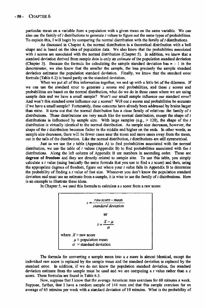
- 50 - CHAPTER 6
particular mean on a variable from a population with a given mean on the same variable. We canalso use the family of t distributions to generate t values to figure out the same types of probabilities.To explain this, I will begin by comparing the normal distribution with the family of t distributions.
As discussed in Chapter 4, the normal distribution is a theoretical distribution with a bellshape and is based on the idea of population data. We also know that the probabilities associatedwith z scores are associated with the normal distribution (Chapter 5). In addition, we know that astandard deviation derived from sample data is only an estimate of the population standard deviation(Chapter 3). Because the formula for calculating the sample standard deviation has n - 1 in thedenominator, we also know that the smaller the sample, the less precisely the sample standarddeviation estimates the population standard deviation. Finally, we know that the standard errorformula (Table 6.2) is based partly on the standard deviation.
When we put all of this information together, we end up with a little bit of the dilemma. Ifwe can use the standard error to generate z scores and probabilities, and these z scores andprobabilities are based on the normal distribution, what do we do in those cases where we are usingsample data and we have a small sample? Won't our small sample influence our standard error?And won't this standard error influence our z scores? Will our z scores and probabilities be accurateif we have a small sample? Fortunately, these concerns have already been addressed by brains largerthan mine. It turns out that the normal distribution has a close family of relatives: the family of tdistributions. These distributions are very much like the normal distribution, except the shape of tdistributions is influenced by sample size. With large samples (e.g., > 120), the shape of the tdistribution is virtually identical to the normal distribution. As sample size decreases, however, theshape of the t distribution becomes flatter in the middle and higher on the ends. In other words, assample size decreases, there will be fewer cases near the mean and more cases away from the mean,out in the tails of the distribution. Like the normal distribution, t distributions are still symmetrical.
Just as we use the z table (Appendix A) to find probabilities associated with the normaldistribution, we use the table of t values (Appendix B) to find probabilities associated with the tdistributions. Along the left column of Appendix B are numbers in ascending order. These aredegrees of freedom and they are directly related to sample size. To use this table, you simplycalculate a t value (using basically the same formula that you use to find a z score) and then, usingthe appropriate degrees of freedom, figure out where your t value falls in Appendix B to determinethe probability of finding a t value of that size. Whenever you don't know the population standarddeviation and must use an estimate from a sample, it is wise to use the family of t distributions. Hereis an example to illustrate these ideas.
In Chapter 5, we used this formula to calculate a z score from a raw score:
z = .raw score - mean
standard deviation
where X= raw scoreu = population mean
a = standard deviation
The formula for converting a sample mean into a z score is almost identical, except theindividual raw score is replaced by the sample mean and the standard deviation is replaced by thestandard error. In addition, if we do not know the population standard deviation, the standarddeviation estimate from the sample must be used and we are computing a t value rather than a zscore. These formulas are found in Table 6.3.
Now, suppose that I know that the average American man exercises for 60 minutes a week.Suppose, further, that I have a random sample of 144 men and that this sample exercises for anaverage of 65 minutes per week with a standard deviation of 10 minutes. What is the probability of
or
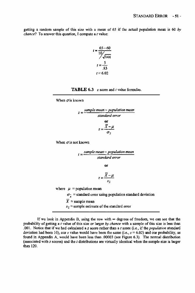
STANDARD ERROR - 51 -
getting a random sample of this size with a mean of 65 if the actual population mean is 60 bychancel To answer this question, I compute a t value:
TABLE 6.3 z score and t value formulas.
When a is known
When a is not known
sample mean — population meant =
standard error
or
where u = population mean(7- = standard error using population standard deviation
X - sample meanS -x = sample estimate of the standard error
If we look in Appendix B, using the row with °° degrees of freedom, we can see that theprobability of getting a t value of this size or larger by chance with a sample of this size is less than.001. Notice that if we had calculated a z score rather than a t score (i.e., if the population standarddeviation had been 10), our z value would have been the same (i.e., z = 6.02) and our probability, asfound in Appendix A, would have been less than .00003 (see Figure 6.3). The normal distribution(associated with z scores) and the t distributions are virtually identical when the sample size is largerthan 120.
sample mean - population meanz =
standard error
or
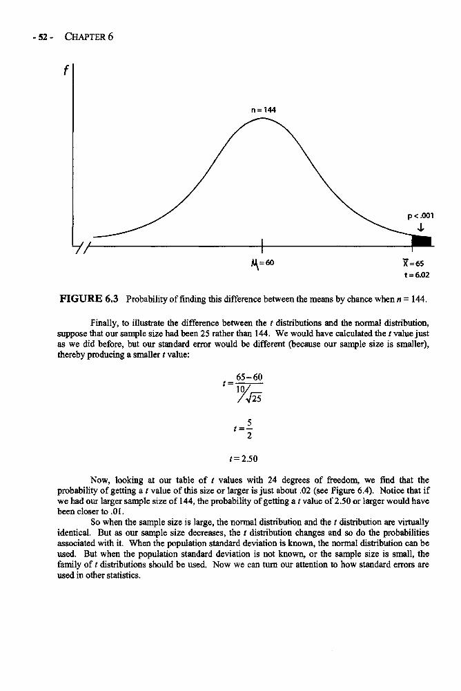
FIGURE 6.3 Probability of finding this difference between the means by chance when n - 144.
Finally, to illustrate the difference between the t distributions and the normal distribution,suppose that our sample size had been 25 rather than 144. We would have calculated the t value justas we did before, but our standard error would be different (because our sample size is smaller),thereby producing a smaller t value:
Now, looking at our table of t values with 24 degrees of freedom, we find that theprobability of getting a t value of this size or larger is just about .02 (see Figure 6.4). Notice that ifwe had our larger sample size of 144, the probability of getting a t value of 2.50 or larger would havebeen closer to .01.
So when the sample size is large, the normal distribution and the t distribution are virtuallyidentical. But as our sample size decreases, the t distribution changes and so do the probabilitiesassociated with it. When the population standard deviation is known, the normal distribution can beused. But when the population standard deviation is not known, or the sample size is small, thefamily of t distributions should be used. Now we can turn our attention to how standard errors areused in other statistics.
- 52 - CHAPTER 6
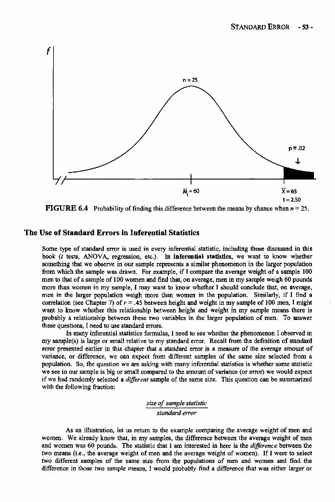
STANDARD ERROR - 53 -
FIGURE 6.4 Probability of finding this difference between the means by chance when n = 25.
The Use of Standard Errors in Inferential Statistics
Some type of standard error is used in every inferential statistic, including those discussed in thisbook (t tests, ANOVA, regression, etc.). In inferential statistics, we want to know whethersomething that we observe in our sample represents a similar phenomenon in the larger populationfrom which the sample was drawn. For example, if I compare the average weight of a sample 100men to that of a sample of 100 women and find that, on average, men in my sample weigh 60 poundsmore than women in my sample, I may want to know whether I should conclude that, on average,men in the larger population weigh more than women in the population. Similarly, if I find acorrelation (see Chapter 7) of r — .45 between height and weight in my sample of 100 men, I mightwant to know whether this relationship between height and weight in my sample means there isprobably a relationship between these two variables in the larger population of men. To answerthese questions, I need to use standard errors.
In many inferential statistics formulas, I need to see whether the phenomenon I observed inmy sample(s) is large or small relative to my standard error. Recall from the definition of standarderror presented earlier in this chapter that a standard error is a measure of the average amount ofvariance, or difference, we can expect from different samples of the same size selected from apopulation. So, the question we are asking with many inferential statistics is whether some statisticwe see in our sample is big or small compared to the amount of variance (or error) we would expectif we had randomly selected a different sample of the same size. This question can be summarizedwith the following fraction:
size of sample statistic
standard error
As an illustration, let us return to the example comparing the average weight of men andwomen. We already know that, in my samples, the difference between the average weight of menand women was 60 pounds. The statistic that I am interested in here is the difference between thetwo means (i.e., the average weight of men and the average weight of women). If I were to selecttwo different samples of the same size from the populations of men and women and find thedifference in those two sample means, I would probably find a difference that was either larger or
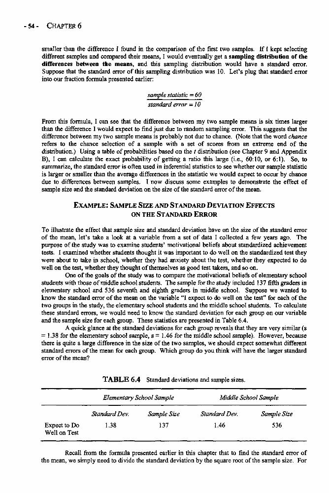
- 54 - CHAPTER 6
smaller than the difference I found in the comparison of the first two samples. If I kept selectingdifferent samples and compared their means, I would eventually get a sampling distribution of thedifferences between the means, and this sampling distribution would have a standard error.Suppose that the standard error of this sampling distribution was 10. Let's plug that standard errorinto our fraction formula presented earlier:
sample statistic = 60
standard error = 10
From this formula, I can see that the difference between my two sample means is six times largerthan the difference I would expect to find just due to random sampling error. This suggests that thedifference between my two sample means is probably not due to chance. (Note that the word chancerefers to the chance selection of a sample with a set of scores from an extreme end of thedistribution.) Using a table of probabilities based on the t distribution (see Chapter 9 and AppendixB), I can calculate the exact probability of getting a ratio this large (i.e., 60:10, or 6:1). So, tosummarize, the standard error is often used in inferential statistics to see whether our sample statisticis larger or smaller than the average differences in the statistic we would expect to occur by chancedue to differences between samples. I now discuss some examples to demonstrate the effect ofsample size and the standard deviation on the size of the standard error of the mean.
EXAMPLE: SAMPLE SIZE AND STANDARD DEVIATION EFFECTSON THE STANDARD ERROR
To illustrate the effect that sample size and standard deviation have on the size of the standard errorof the mean, let's take a look at a variable from a set of data I collected a few years ago. Thepurpose of the study was to examine students' motivational beliefs about standardized achievementtests. I examined whether students thought it was important to do well on the standardized test theywere about to take in school, whether they had anxiety about the test, whether they expected to dowell on the test, whether they thought of themselves as good test takers, and so on.
One of the goals of the study was to compare the motivational beliefs of elementary schoolstudents with those of middle school students. The sample for the study included 137 fifth graders inelementary school and 536 seventh and eighth graders in middle school. Suppose we wanted toknow the standard error of the mean on the variable "I expect to do well on the test" for each of thetwo groups in the study, the elementary school students and the middle school students. To calculatethese standard errors, we would need to know the standard deviation for each group on our variableand the sample size for each group. These statistics are presented in Table 6.4.
A quick glance at the standard deviations for each group reveals that they are very similar (s= 1.38 for the elementary school sample, s = 1.46 for the middle school sample). However, becausethere is quite a large difference in the size of the two samples, we should expect somewhat differentstandard errors of the mean for each group. Which group do you think will have the larger standarderror of the mean?
TABLE 6.4 Standard deviations and sample sizes.
Elementary School Sample Middle School Sample
Expect to DoWell on Test
Standard Dev.
1.38
Sample Size
137
Standard Dev.
1.46
Sample Size
536
Recall from the formula presented earlier in this chapter that to find the standard error ofthe mean, we simply need to divide the standard deviation by the square root of the sample size. For
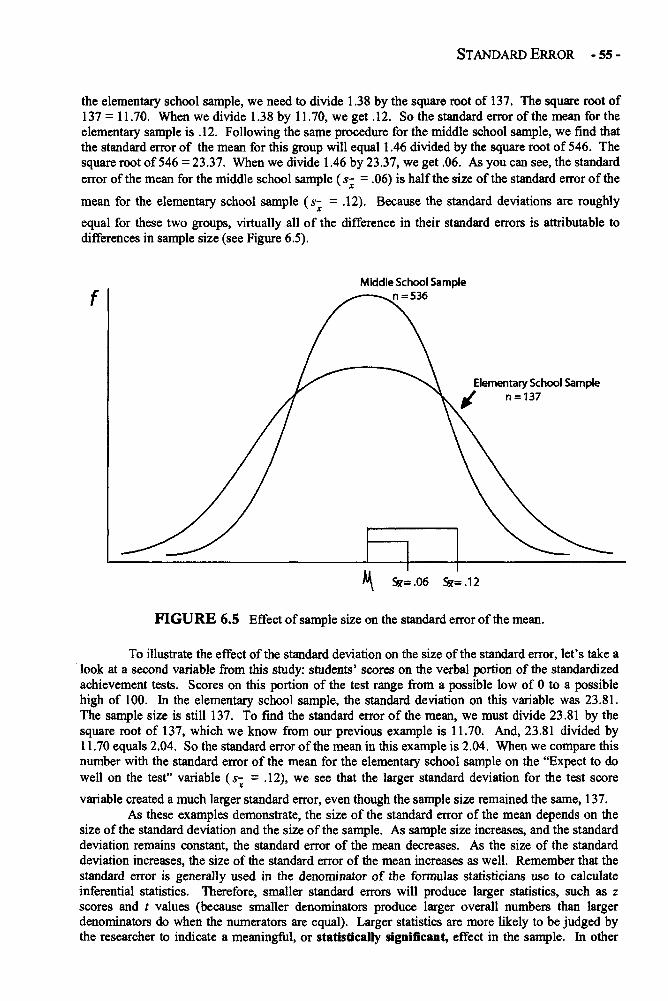
STANDARD ERROR - 55 -
the elementary school sample, we need to divide 1.38 by the square root of 137. The square root of137 = 11.70. When we divide 1.38 by 11.70, we get .12. So the standard error of the mean for theelementary sample is .12. Following the same procedure for the middle school sample, we find thatthe standard error of the mean for this group will equal 1.46 divided by the square root of 546. Thesquare root of 546 = 23.37. When we divide 1.46 by 23.37, we get .06. As you can see, the standarderror of the mean for the middle school sample (s -x = .06) is half the size of the standard error of the
mean for the elementary school sample (s -x = .12). Because the standard deviations are roughly
equal for these two groups, virtually all of the difference in their standard errors is attributable todifferences in sample size (see Figure 6.5).
FIGURE 6.5 Effect of sample size on the standard error of the mean.
To illustrate the effect of the standard deviation on the size of the standard error, let's take alook at a second variable from this study: students' scores on the verbal portion of the standardizedachievement tests. Scores on this portion of the test range from a possible low of 0 to a possiblehigh of 100. In the elementary school sample, the standard deviation on this variable was 23.81.The sample size is still 137. To find the standard error of the mean, we must divide 23.81 by thesquare root of 137, which we know from our previous example is 11.70. And, 23.81 divided by11.70 equals 2.04. So the standard error of the mean in this example is 2.04. When we compare thisnumber with the standard error of the mean for the elementary school sample on the "Expect to dowell on the test" variable (s-x = .12), we see that the larger standard deviation for the test score
variable created a much larger standard error, even though the sample size remained the same, 137.As these examples demonstrate, the size of the standard error of the mean depends on the
size of the standard deviation and the size of the sample. As sample size increases, and the standarddeviation remains constant, the standard error of the mean decreases. As the size of the standarddeviation increases, the size of the standard error of the mean increases as well. Remember that thestandard error is generally used in the denominator of the formulas statisticians use to calculateinferential statistics. Therefore, smaller standard errors will produce larger statistics, such as zscores and t values (because smaller denominators produce larger overall numbers than largerdenominators do when the numerators are equal). Larger statistics are more likely to be judged bythe researcher to indicate a meaningful, or statistically significant, effect in the sample. In other
- 56 - CHAPTER 6
words, a large statistic like a t value or a z score is more likely than small statistics to indicate that aphenomenon observed in a sample represents a meaningful phenomenon in the population as well.(Statistical significance is discussed in greater detail in Chapter 7). Therefore, all else being equal,larger sample sizes are more likely to produce statistically significant results because larger samplesizes produce smaller standard errors.
WRAPPING UP AND LOOKING FORWARD
Standard error is often a difficult concept to grasp the first time it is encountered (or the second orthe third). Because it is such a fundamental concept in inferential statistics, however, I encourageyou to keep trying to make sense of both the meaning and the usefulness of standard errors. As welearned in this chapter, standard errors can be used to determine probabilities of sample statistics(such as the mean) in much the same way that we used standard scores to determine probabilitiesassociated with individual scores in Chapter 4. Because of the usefulness of standard errors indetermining probabilities, standard errors play a critical role in determining whether a statistic isstatistically significant. Because standard errors are influenced by sample size, statisticalsignificance will also be influenced by these sample characteristics. In the next chapter, the issue ofstatistical significance, and the effects of sample size on statistical significance, are discussed inmore depth.
GLOSSARY OF TERMS AND SYMBOLS FOR CHAPTER 6
Central limit theorem: The fact that as sample size increases, the sampling distribution of themean becomes increasingly normal, regardless of the shape of the distribution of thesample.
Degrees of freedom: Roughly, the minimum amount of data needed to calculate a statistic. Morepractically, it is a number, or numbers, used to approximate the number of observations inthe data set for the purpose of determining statistical significance.
Expected value of the mean: The value of the mean one would expect to get from a randomsample selected from a population with a known mean. For example, if one knows thepopulation has a mean of 5 on some variable, one would expect a random sample selectedfrom the population to also have a mean of 5.
Inferential statistics: Statistics generated from sample data that are used to make inferences aboutthe characteristics of the population the sample is alleged to represent.
Sampling distribution of the differences between the means: The distribution of scores thatwould be generated if one were to repeatedly draw two random samples of a given sizefrom two populations and calculate the difference between the sample means.
Sampling distribution of the mean: The distribution of scores that would be generated if one wereto repeatedly draw random samples of a given size from a population and calculate themean for each sample drawn.
Sampling distribution: A theoretical distribution of any statistic that one would get by repeatedlydrawing random samples of a given size from the population and calculating the statistic ofinterest for each sample.
Standard error: The standard deviation of the sampling distribution.Statistically significant: A term indicating that a phenomenon observed in a sample (or samples)
has meaningful implications for the population (e.g., that the difference between a samplemean and a population mean is statistically significant or that a relationship observedbetween two variables in a sample is strong enough, relative to the standard error, toindicate a relationship between the two variables in the population from which the samplewas selected).
s-x The standard error of the mean estimated from the sample standard deviation (i.e., when the
population standard deviation is unknown).a-x The standard error of the mean when the population standard deviation is known.
CHAPTER 7
STATISTICAL SIGNIFICANCE, EFFECT SIZE,AND CONFIDENCE INTERVALS
When researchers use the data collected from samples to make inferences about the population (orpopulations) from which the samples were selected, they need to have some way of deciding howmeaningful the sample data are. Are the differences between two samples (e.g., a group of adultsfrom Alaska and a group of adults from New York) in their average levels of happiness large enoughto conclude that the populations of adults from these two states actually differ in how happy theyare? Is the relationship between years of education and income among a sample of 50 Americanadults strong enough to determine that income is related to education in the larger population ofAmerican adults? How do researchers reach important conclusions about how well sample statisticsgeneralize to the larger population?
Three of the common tools used by researchers to reach such conclusions include testingfor statistical significance and calculating the effect sizes and confidence intervals. All of thesetools provide indexes of how meaningful the results of statistical analyses are. Despite their frequentappearance in reports of quantitative research (particularly measures of statistical significance), theseconcepts are poorly understood by many researchers. The purpose of this chapter is to provide you,the reader, with a solid foundation of the concepts of statistical significance, effect size, andconfidence intervals. Because statistical significance, effect size, and confidence intervals can becalculated for virtually any statistic, it is not possible in this short chapter to provide instructions onhow to determine statistical significance or calculate an effect size or confidence interval across allresearch situations. Therefore, the focus of this chapter is to describe what these concepts mean andhow to interpret them, as well as to provide general information about how statistical significanceand effect sizes are determined.
Statistics are often divided into two types: descriptive statistics and inferential statistics.As I mentioned in Chapter 1, descriptive statistics are those statistics that describe the characteristicsof a given set of data. For example, if I collect weight data for a group of 30 adults, I can use avariety of statistics to describe the weight characteristics of these 30 adults (e.g., their average, ormean, weight, the range from the lowest to the highest weight, the standard deviation for this group,etc.). Notice that all of these descriptive statistics do nothing more than provide information aboutthis specific group of 30 individuals from whom I collected data.
Although descriptive statistics are useful and important, researchers are often interested inextending their results beyond the specific group of people from whom they have collected data (i.e.,their sample, or samples). From their sample data, researchers often want to determine whetherthere is some phenomenon of interest occurring in the larger population(s) that these samplesrepresent. For example, I may want to know whether, in the general population, boys and girls differin their levels of physical aggression. To determine this, I could conduct a study in which I measurethe physical aggression levels of every boy and girl in the United States and see whether boys andgirls differ. This study would be very costly, however, and very time consuming. Another approachis to select a sample of boys and a sample of girls, measure their levels of physical aggression, see ifthey differ, and from these sample data infer about differences in the larger populations of boys andgirls. If I eventually conclude that my results are statistically significant, in essence I am concludingthat the differences I observed in the average levels of aggression of the boys and girls in my twosamples represent a likelihood that there is also a difference in the average levels of aggression in thepopulations of boys and girls from which these samples were selected.
As the name implies, inferential statistics are always about making inferences about the
-57-
- 58 - CHAPTER 7
larger population(s) on the basis of data collected from a sample or samples. To understand how thisworks, we first need to understand the distinction between a population and a sample and getcomfortable with some concepts from probability. Once we have developed an understanding ofstatistical significance, we can then compare the concepts of statistical significance and practicalsignificance. This distinction leads us to the second major concept covered in this chapter, which iseffect size. Briefly, effect size is a measure of how large an observed effect is without regard to thesize of the sample. In the earlier example examining levels of aggression, the effect that I aminterested in is the difference in boys' and girls' average levels of aggression. Finally, we cancalculate a confidence interval to provide a range of values that we are confident, to a certain degreeof probability, contain the actual population parameter.
STATISTICAL SIGNIFICANCE IN DEPTH
Samples and Populations
The first step in understanding statistical significance is to understand the difference between asample and a population. This difference has been discussed earlier (Chapter 1). Briefly, a sampleis an individual or group from whom or from which data are collected. A population is theindividual or group that the sample is supposed to represent. For the purposes of understanding theconcept of statistical significance, it is critical that you remember that when researchers collect datafrom a sample, they are often interested in using these data to make inferences about the populationfrom which the sample was drawn. Statistical significance refers to the likelihood, or probability,that a statistic derived from a sample represents some genuine phenomenon in the population fromwhich the sample was selected. In other words, statistical significance provides a measure to help usdecide whether what we observe in our sample is also going on in the population that the sample issupposed to represent.
One factor that often complicates this process of making inferences from the sample to thepopulation is that in many, if not most, research studies in the social sciences, the population is neverexplicitly defined. This is somewhat problematic, because when we argue that a statistical result isstatistically significant, we are essentially arguing that the result we found in our sample isrepresentative of some effect in the population from which the sample was selected. If we have notadequately defined our population, it is not entirely clear what to make of such a result (see Chapter1 for a more detailed discussion of defining populations). For the purposes of this chapter, however,suffice it to say that samples are those individuals or groups from whom or which data are collected,whereas populations are the entire collection of individuals or cases from which the samples areselected.
Probability
As discussed earlier in Chapter 4 and Chapter 6, probability plays a key role in inferential statistics.When it comes to deciding whether a result in a study is statistically significant, we must rely onprobability to make the determination. Here is how it works.
When we calculate an inferential statistic, that statistic is part of a sampling distribution.From our discussion of standard errors in Chapter 6, you will recall that whenever we select asample from a population and calculate a statistic from the sample, we have to keep in mind that ifwe had selected a different sample of the same size from the same population, we probably wouldget a slightly different statistic from the new sample. For example, if I randomly selected a sampleof 1,000 men from the population of men in the United States and measured their shoe size, I mightfind an average shoe size of 10 for this sample. Now, if I were to randomly select a new sample of1,000 men from the population of men in the United States and calculate their average shoe size, Imight get a different mean, such as 9. If I were to select an infinite number of random samples of1,000 and calculate the average shoe sizes of each of these samples, I would end up with a samplingdistribution of the mean, and this sampling distribution would have a standard deviation, called thestandard error of the mean (see Chapter 6 for a review of this concept). Just as there is a samplingdistribution and a standard error of the mean, so there are sampling distributions and standard errors
MEASURES OF EFFECTS - 59 -
for all statistics, including correlation coefficients, F ratios from ANOVA, t values from t tests,regression coefficients, and so on.
Because these sampling distributions have certain stable mathematical characteristics, wecan use the standard errors to calculate the exact probability of obtaining a specific sample statistic,from a sample of a given size, using a specific known or hypothesized population parameter. It'stime for an example. Suppose that, from previous research by the shoe industry, I know that theaverage shoe size for the population of men in the United States is a size 9. Because this is theknown average for the population, this average is a parameter and not a statistic. Now suppose Irandomly select a sample of 1,000 men and find that their average shoe size is 10, with a standarddeviation of 2. Notice that the average for my sample (10) is a statistic because it comes from mysample, not my population. With these numbers, I can answer two slightly different but relatedquestions. First, if the average shoe size in the population is really 9, what is the probability ofselecting a random sample of 1,000 men who have an average shoe size of 10? Second, is thedifference between my population mean (9) and my sample mean (10) statistically significant? Theanswer to my first question provides the basis for the answer to my second question. Notice thatsimply by looking at the two means, I can clearly see that they are different (i.e., 9 is different from10). So I am trying to answer a deeper question than whether they differ. Rather, I am trying todetermine whether the difference between my sample and population means is statisticallysignificant. In other words, I am trying to determine whether the difference between my sample andpopulations means is too large to likely have occurred by chance (i.e., who I happened to get in mysample).
Notice that if I do not select my sample at random, it would be easy to find a sample of1,000 men with an average shoe size of 10. I could buy customer lists from shoe stores and select1,000 men who bought size 10 shoes. Or I could place an advertisement in the paper seeking menwho wear a size 10 shoe. But if my population mean is really 9, and my sample is really selected atrandom, then there is some probability, or chance, that I could wind up with a sample of 1,000 menwith an average shoe size of 10. In statistics, this chance is referred is as random sampling erroror random chance.
Back to the example. If my population mean is 9, and my random sample of 1,000 men hasa mean of 10 and a standard deviation of 2, I can calculate the standard error by dividing thestandard deviation by the square root of the sample size (see Chapter 6 for this formula).
Where sx = the standard error of the mean
Now that I know the standard error is .06, I can calculate a t value to find the approximateprobability of getting a sample mean of 10 by random chance if the population mean is really 9.(Note: For sample sizes larger than 120, the t distribution is identical to the normal distribution.Therefore, for large sample sizes, t values and z values, and their associated probabilities, arevirtually identical. See Chapters 4 and 6 for more information.)
When using the t distribution to find probabilities, we can simply take the absolute value oft. Once we have our absolute value for t (t = 16.67), we can consult the t table in Appendix B andsee that, when the degrees of freedom equal infinity (i.e., greater than 120), the probability of gettinga t value of 16.67 or greater is less than .001. In fact, because the critical t value associated with a
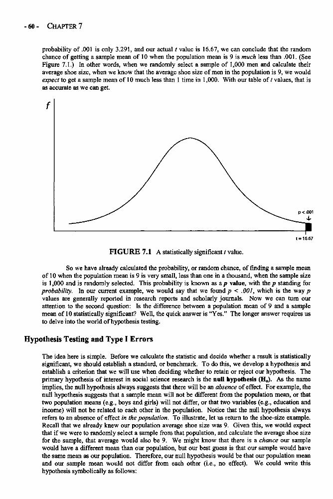
- 60 - CHAPTER 7
probability of .001 is only 3.291, and our actual t value is 16.67, we can conclude that the randomchance of getting a sample mean of 10 when the population mean is 9 is much less than .001. (SeeFigure 7.1.) In other words, when we randomly select a sample of 1,000 men and calculate theiraverage shoe size, when we know that the average shoe size of men in the population is 9, we wouldexpect to get a sample mean of 10 much less than 1 time in 1,000. With our table of t values, that isas accurate as we can get.
FIGURE 7.1 A statistically significant t value.
So we have already calculated the probability, or random chance, of finding a sample meanof 10 when the population mean is 9 is very small, less than one in a thousand, when the sample sizeis 1,000 and is randomly selected. This probability is known as .p value, with the p standing forprobability. In our current example, we would say that we found p < .001, which is the way pvalues are generally reported in research reports and scholarly journals. Now we can turn ourattention to the second question: Is the difference between a population mean of 9 and a samplemean of 10 statistically significant? Well, the quick answer is "Yes." The longer answer requires usto delve into the world of hypothesis testing.
Hypothesis Testing and Type I Errors
The idea here is simple. Before we calculate the statistic and decide whether a result is statisticallysignificant, we should establish a standard, or benchmark. To do this, we develop a hypothesis andestablish a criterion that we will use when deciding whether to retain or reject our hypothesis. Theprimary hypothesis of interest in social science research is the null hypothesis (H1). As the nameimplies, the null hypothesis always suggests that there will be an absence of effect. For example, thenull hypothesis suggests that a sample mean will not be different from the population mean, or thattwo population means (e.g., boys and girls) will not differ, or that two variables (e.g., education andincome) will not be related to each other in the population. Notice that the null hypothesis alwaysrefers to an absence of effect in the population. To illustrate, let us return to the shoe-size example.Recall that we already knew our population average shoe size was 9. Given this, we would expectthat if we were to randomly select a sample from that population, and calculate the average shoe sizefor the sample, that average would also be 9. We might know that there is a chance our samplewould have a different mean than our population, but our best guess is that our sample would havethe same mean as our population. Therefore, our null hypothesis would be that our population meanand our sample mean would not differ from each other (i.e., no effect). We could write thishypothesis symbolically as follows:
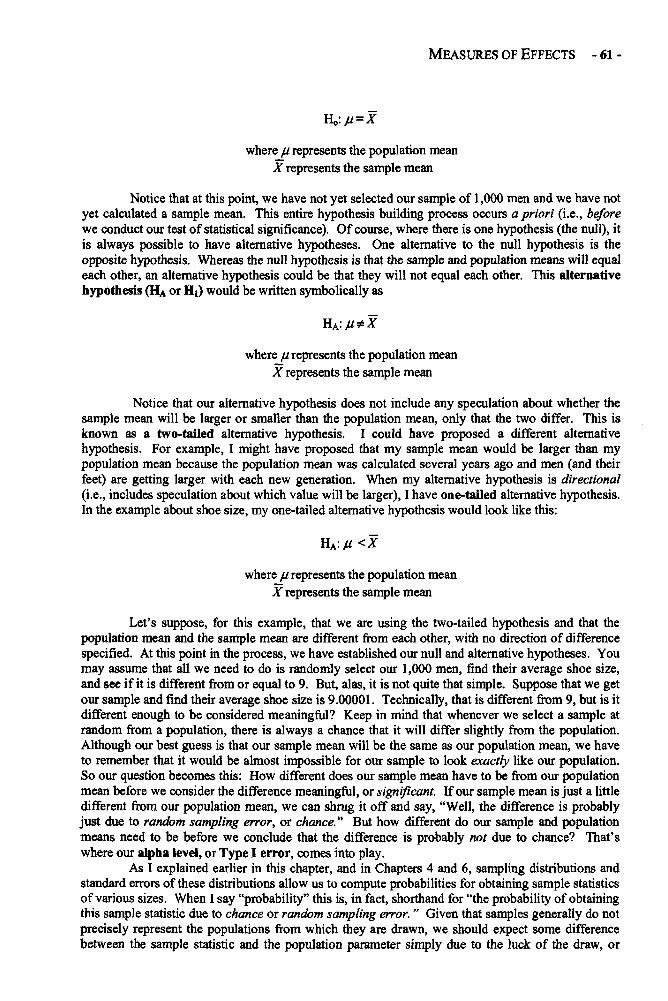
MEASURES OF EFFECTS - 61 -
where u represents the population meanX represents the sample mean
Notice that at this point, we have not yet selected our sample of 1,000 men and we have notyet calculated a sample mean. This entire hypothesis building process occurs a priori (i.e., beforewe conduct our test of statistical significance). Of course, where there is one hypothesis (the null), itis always possible to have alternative hypotheses. One alternative to the null hypothesis is theopposite hypothesis. Whereas the null hypothesis is that the sample and population means will equaleach other, an alternative hypothesis could be that they will not equal each other. This alternativehypothesis (HA or H1) would be written symbolically as
where urepresents the population meanX represents the sample mean
Notice that our alternative hypothesis does not include any speculation about whether thesample mean will be larger or smaller than the population mean, only that the two differ. This isknown as a two-tailed alternative hypothesis. I could have proposed a different alternativehypothesis. For example, I might have proposed that my sample mean would be larger than mypopulation mean because the population mean was calculated several years ago and men (and theirfeet) are getting larger with each new generation. When my alternative hypothesis is directional(i.e., includes speculation about which value will be larger), I have one-tailed alternative hypothesis.In the example about shoe size, my one-tailed alternative hypothesis would look like this:
H: u < x w h e r e u represents t he population meanX represents the sample mean
Let's suppose, for this example, that we are using the two-tailed hypothesis and that thepopulation mean and the sample mean are different from each other, with no direction of differencespecified. At this point in the process, we have established our null and alternative hypotheses. Youmay assume that all we need to do is randomly select our 1,000 men, find their average shoe size,and see if it is different from or equal to 9. But, alas, it is not quite that simple. Suppose that we getour sample and find their average shoe size is 9.00001. Technically, that is different from 9, but is itdifferent enough to be considered meaningful? Keep in mind that whenever we select a sample atrandom from a population, there is always a chance that it will differ slightly from the population.Although our best guess is that our sample mean will be the same as our population mean, we haveto remember that it would be almost impossible for our sample to look exactly like our population.So our question becomes this: How different does our sample mean have to be from our populationmean before we consider the difference meaningful, or significant. If our sample mean is just a littledifferent from our population mean, we can shrug it off and say, "Well, the difference is probablyjust due to random sampling error, or chance" But how different do our sample and populationmeans need to be before we conclude that the difference is probably not due to chance? That'swhere our alpha level, or Type I error, comes into play.
As I explained earlier in this chapter, and in Chapters 4 and 6, sampling distributions andstandard errors of these distributions allow us to compute probabilities for obtaining sample statisticsof various sizes. When I say "probability" this is, in fact, shorthand for "the probability of obtainingthis sample statistic due to chance or random sampling error. " Given that samples generally do notprecisely represent the populations from which they are drawn, we should expect some differencebetween the sample statistic and the population parameter simply due to the luck of the draw, or
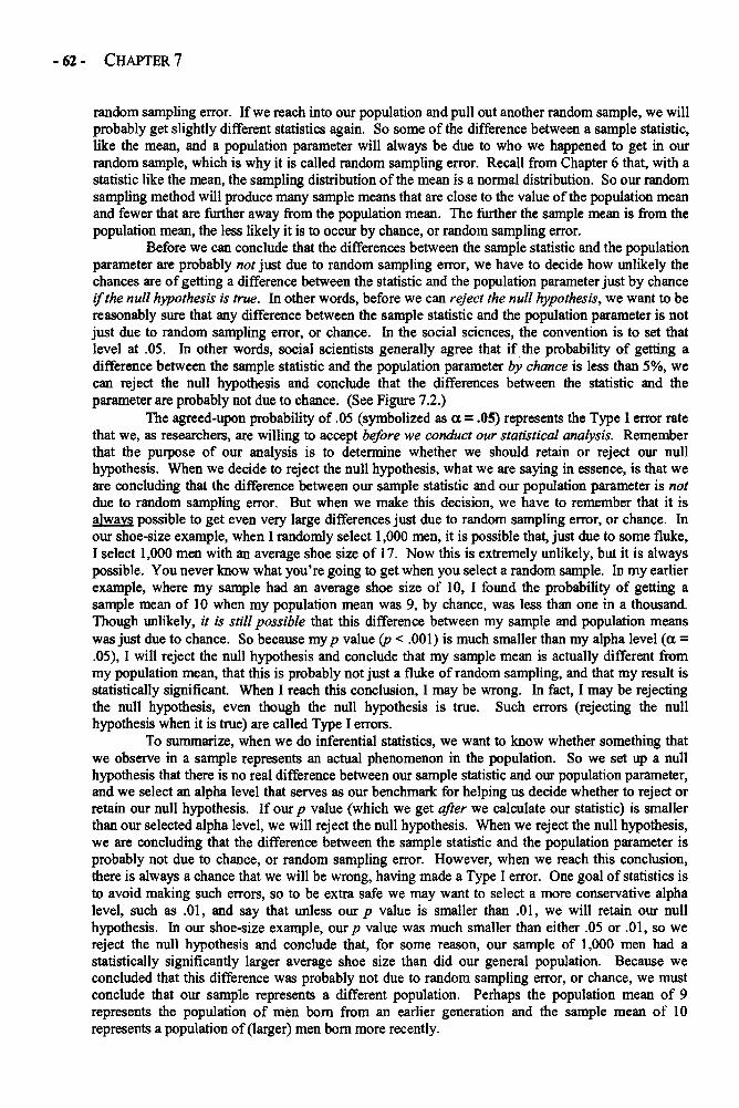
- 62 - CHAPTER 7
random sampling error. If we reach into our population and pull out another random sample, we willprobably get slightly different statistics again. So some of the difference between a sample statistic,like the mean, and a population parameter will always be due to who we happened to get in ourrandom sample, which is why it is called random sampling error. Recall from Chapter 6 that, with astatistic like the mean, the sampling distribution of the mean is a normal distribution. So our randomsampling method will produce many sample means that are close to the value of the population meanand fewer that are further away from the population mean. The further the sample mean is from thepopulation mean, the less likely it is to occur by chance, or random sampling error.
Before we can conclude that the differences between the sample statistic and the populationparameter are probably not just due to random sampling error, we have to decide how unlikely thechances are of getting a difference between the statistic and the population parameter just by chanceif the null hypothesis is true. In other words, before we can reject the null hypothesis, we want to bereasonably sure that any difference between the sample statistic and the population parameter is notjust due to random sampling error, or chance. In the social sciences, the convention is to set thatlevel at .05. In other words, social scientists generally agree that if the probability of getting adifference between the sample statistic and the population parameter by chance is less than 5%, wecan reject the null hypothesis and conclude that the differences between the statistic and theparameter are probably not due to chance. (See Figure 7.2.)
The agreed-upon probability of .05 (symbolized as a = .05) represents the Type I error ratethat we, as researchers, are willing to accept before we conduct our statistical analysis. Rememberthat the purpose of our analysis is to determine whether we should retain or reject our nullhypothesis. When we decide to reject the null hypothesis, what we are saying in essence, is that weare concluding that the difference between our sample statistic and our population parameter is notdue to random sampling error. But when we make this decision, we have to remember that it isalways possible to get even very large differences just due to random sampling error, or chance. Inour shoe-size example, when I randomly select 1,000 men, it is possible that, just due to some fluke,I select 1,000 men with an average shoe size of 17. Now this is extremely unlikely, but it is alwayspossible. You never know what you're going to get when you select a random sample. In my earlierexample, where my sample had an average shoe size of 10, I found the probability of getting asample mean of 10 when my population mean was 9, by chance, was less than one in a thousand.Though unlikely, it is still possible that this difference between my sample and population meanswas just due to chance. So because my p value (p < .001) is much smaller than my alpha level (a =.05), I will reject the null hypothesis and conclude that my sample mean is actually different frommy population mean, that this is probably not just a fluke of random sampling, and that my result isstatistically significant. When I reach this conclusion, I may be wrong. In fact, I may be rejectingthe null hypothesis, even though the null hypothesis is true. Such errors (rejecting the nullhypothesis when it is true) are called Type I errors.
To summarize, when we do inferential statistics, we want to know whether something thatwe observe in a sample represents an actual phenomenon in the population. So we set up a nullhypothesis that there is no real difference between our sample statistic and our population parameter,and we select an alpha level that serves as our benchmark for helping us decide whether to reject orretain our null hypothesis. If our p value (which we get after we calculate our statistic) is smallerthan our selected alpha level, we will reject the null hypothesis. When we reject the null hypothesis,we are concluding that the difference between the sample statistic and the population parameter isprobably not due to chance, or random sampling error. However, when we reach this conclusion,there is always a chance that we will be wrong, having made a Type I error. One goal of statistics isto avoid making such errors, so to be extra safe we may want to select a more conservative alphalevel, such as .01, and say that unless our p value is smaller than .01, we will retain our nullhypothesis. In our shoe-size example, our p value was much smaller than either .05 or .01, so wereject the null hypothesis and conclude that, for some reason, our sample of 1,000 men had astatistically significantly larger average shoe size than did our general population. Because weconcluded that this difference was probably not due to random sampling error, or chance, we mustconclude that our sample represents a different population. Perhaps the population mean of 9represents the population of men born from an earlier generation and the sample mean of 10represents a population of (larger) men born more recently.
MEASURES OF EFFECTS - 63 -
FIGURE 7.2 Regions of rejection for a two-tailed test.
FIGURE 7.3 Region of rejection for a one-tailed test.
EFFECT SIZE IN DEPTH
As an indication of the importance of a result in quantitative research, statistical significance hasenjoyed a rather privileged position for decades. Social scientists have long given the "p < .05" rulea sort of magical quality, with any result carrying a probability greater than .05 being quicklydiscarded into the trash heap of "nonsignificant" results. Recently, however, researchers and journaleditors have begun to view statistical significance in a slightly less flattering light, recognizing oneof its major shortcomings: It is perhaps too heavily influenced by sample size. As a result, more andmore researchers are becoming aware of the importance of effect size and increasingly are including
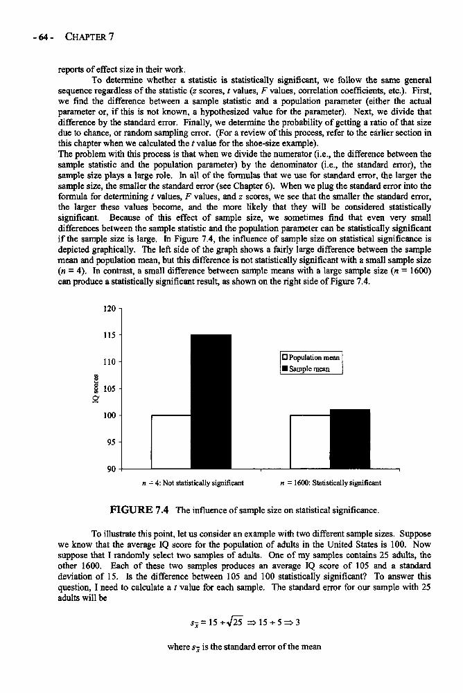
- 64 - CHAPTER 7
reports of effect size in their work.To determine whether a statistic is statistically significant, we follow the same general
sequence regardless of the statistic (z scores, t values, F values, correlation coefficients, etc.). First,we find the difference between a sample statistic and a population parameter (either the actualparameter or, if this is not known, a hypothesized value for the parameter). Next, we divide thatdifference by the standard error. Finally, we determine the probability of getting a ratio of that sizedue to chance, or random sampling error. (For a review of this process, refer to the earlier section inthis chapter when we calculated the t value for the shoe-size example).The problem with this process is that when we divide the numerator (i.e., the difference between thesample statistic and the population parameter) by the denominator (i.e., the standard error), thesample size plays a large role. In all of the formulas that we use for standard error, the larger thesample size, the smaller the standard error (see Chapter 6). When we plug the standard error into theformula for determining t values, F values, and z scores, we see that the smaller the standard error,the larger these values become, and the more likely that they will be considered statisticallysignificant. Because of this effect of sample size, we sometimes find that even very smalldifferences between the sample statistic and the population parameter can be statistically significantif the sample size is large. In Figure 7.4, the influence of sample size on statistical significance isdepicted graphically. The left side of the graph shows a fairly large difference between the samplemean and population mean, but this difference is not statistically significant with a small sample size(n = 4). In contrast, a small difference between sample means with a large sample size (n = 1600)can produce a statistically significant result, as shown on the right side of Figure 7.4.
FIGURE 7.4 The influence of sample size on statistical significance.
To illustrate this point, let us consider an example with two different sample sizes. Supposewe know that the average IQ score for the population of adults in the United States is 100. Nowsuppose that I randomly select two samples of adults. One of my samples contains 25 adults, theother 1600. Each of these two samples produces an average IQ score of 105 and a standarddeviation of 15. Is the difference between 105 and 100 statistically significant? To answer thisquestion, I need to calculate a / value for each sample. The standard error for our sample with 25adults will be
s, = l5+j25 =15 + 5=>3
where s~ is the standard error of the mean
MEASURES OF EFFECTS - 65 -
The standard error for our second sample, with 1,600 adults, will be
sx = 15 + A/1600 => 15 + 40 => .375
Plugging these standard errors into our t value formulas, we find that the t value for the 25-person sample is (105 - 100) + 3, or 1.67. Looking in our table of t distributions (Appendix B), wecan see that the p value for a t value of 1.67 is between .10 and .20. The t value for the sample with1,600 adults is (105 - 100) + .375, or 13.33, with a corresponding p value of p < .0001. If we areusing an alpha level of .05, then a difference of 5 points on the IQ test would not be consideredstatistically significant if we only had a sample size of 25, but would be highly statisticallysignificant if our sample size were 1,600. Because sample size plays such a big role in determiningstatistical significance, many statistics textbooks make a distinction between statistical significanceand practical significance. With a sample size of 1,600, a difference of even 1 point on the IQ testwould produce a statistically significant result (t = 1 + .375 => t - 2.67, p < .01). However, if we hada very small sample size of 4, even a 15-point difference in average IQ scores would not bestatistically significant (t = 15 + 7.50 => t = 2.00, p > .10). (See Figure 7.3 for a graphic illustrationof this.) But is a difference of 1 point on a test with a range of over 150 points really important inthe real world? And is a difference of 15 points not meaningful? In other words, is it a significantdifference in the practical sense of the word significant? One way to answer this question is toexamine the effect size.
There are different formulas for calculating the effect sizes of different statistics, but theseformulas share common features. The formulas for calculating most inferential statistics involve aratio of a numerator (such as the difference between a sample mean and a population mean in a one-sample t test) divided by a standard error. Similarly, most effect size formulas use the samenumerator, but divide this numerator by a standard deviation rather than a standard error. The trick,then, is knowing how to come up with the appropriate standard deviation to use in a particular effectsize formula.
We can examine the simplest form of effect size by returning to our examples using IQscores. Remember that we have a population with an average IQ score of 100. We also had twosamples, each with an average IQ score of 105 and a standard deviation of 15; one with a samplesize of 25 and the other with a sample size of 1,600. Also recall that to find the standard error forcalculating our t scores, we simply divided the standard deviation by the square root of the samplesize. So for the sample with 25 members, our standard error was
Sx = l5+j25 =>15+-5=>3
where s-= is the standard error of the mean' X
To calculate an effect size, what we need to do is convert this standard error back into astandard deviation. If we divide the standard deviation by the square root of the sample size to findthe standard error, we can multiply the standard error by the square root of the sample size to find thestandard deviation. When we do this, we find that
s = 3-j25 = > 3 x 5 = > 1 5
where s is the sample standard deviation
Notice that the standard deviation would be exactly the same if we calculated it for the larger samplesize of 1,600, even though the standard error was much smaller for that sample.
s = .375 V1600 => .375 x 40 => 15
Once we have our standard deviation, it is easy to calculate an effect size, which has the
- 66 - CHAPTER 7
symbol d. In the IQ example, we could determine the effect size as follows:
where d is the effect size
As you can see, the formula for the effect size translates the numerator into standarddeviation units. When the numerator represents some sort of difference score (e.g., the differencebetween two or more group means, the difference between a sample statistic and a populationparameter), the effect size will represent that difference in standard deviation units. This is similar torepresenting the difference in standard error units, as most inferential statistics do (e.g., t values, Fvalues, correlation coefficients), except that sample size is eliminated from the process.
There are no hard and fast rules regarding the interpretation of effect sizes. Some textbookauthors suggest that effect sizes smaller than .20 are small, those between .25 and .75 are moderate,and those over .80 are large. When determining whether an effect size is meaningful, it is importantto consider what you are testing and what your perspective is. If I am comparing the mortality ratesof two samples trying two different experimental drugs, even small effect sizes are important,because we are talking about life and death. But if I'm comparing two different samples' preferencefor ice cream flavors, even fairly large effect sizes may have little more than trivial importance tomost people.4 Keep in mind, however, that what is trivial to one person may be vitally important toanother. Although I do not care about even large differences in people's preference for certain icecream flavors, the CEO of an ice cream company may care very much about even small differencesin preference. In fact, a small preference for chocolate over vanilla can mean millions of dollars toan ice cream company (and the owners of stock in the company). The point here is that "practicalsignificance" is a subjective concept. Although statistics can provide measures of effect size,interpreting the importance of these effect sizes is an imprecise science.
The recent push by some researchers to focus more heavily on effect sizes than onstatistical significance reminds me that I should conclude this section of the chapter by urging you totake both effect size and statistical significance into consideration as you read and conduct research.Notice that in the previous examples, the exact same effect size was produced with the 25-personsample as with the 1,600-person sample. These results suggest that sample size does not matter. Infact, sample size is very important. Stated simply, it is easier to come up with fluke, or chanceresults with smaller sample sizes than with larger sample sizes. Our tests of statistical significance,which are sensitive to sample size, tell us the probability that our results are due to random samplingerror, or chance. Because larger sample sizes have a better likelihood of representing thepopulations from which they were selected, the results of studies that use larger sample sizes aremore reliable than those using smaller sample sizes, if all else is equal (e.g., how the samples wereselected, the methods used in the study, etc.). When used together, tests of statistical significanceand measures of effect size can provide important information regarding the reliability andimportance of statistical results. Of course, our own judgments about the meaning, causes, andconsequences of our results are also important factors.
CONFIDENCE INTERVALS IN DEPTHConfidence intervals are becoming increasingly common in reports of inferential statistics, in partbecause they provide another measure of effect size. When a researcher uses sample data to make
There are other types of effect sizes frequently reported in research. One of the most common of these is the percentage of varianceexplained by the independent variable. I mention this in later chapters as I discuss the concept of explained variance.
MEASURES OF EFFECTS - 67 -
some inference about a population, she usually does not really know the actual value of thepopulation parameter. All she has is her sample data. But using probability and confidenceintervals, she can make an educated prediction about the approximate value of the populationparameter.
To illustrate how confidence intervals work, let's return to the shoe-size example fromearlier in the chapter. But let me slightly rephrase the statement about the average shoe size in thepopulation. Instead of saying, as I did earlier, "In the population of American men, the averageshoes size is 9," let me say, "Suppose that the average shoe size of American men is 9." This istechnically more accurate because, assuming the average shoe size in the population was determinedsome time ago, we do not really know the average shoe size of the current population of Americanmen. So our hypothesized value of the average shoe size in the population is 9, and our observedshoe size in our sample of 1,000 men is 10, with a standard deviation of 2. Using these data, we cancalculate a confidence interval.
Recall that in our earlier example, using the same values for the sample mean, standarddeviation, and sample size, we calculated a standard error of .06. Using these data, we can calculatea confidence interval. The confidence interval provides a range of values that we are confident, to acertain degree of probability, contains the population parameter (e.g., the population mean). Most ofthe time, researchers want to be either 95% or 99% confident that the confidence interval containsthe population parameter. These values correspond with p values of .05 and .01, respectively. Theformulas for calculating 95% and 99% confidence intervals are provided in Table 7.2. Notice thatthe formula for the confidence interval involves building the interval around the sample statistic(both greater than and less than the sample statistic). Because the confidence interval involvesvalues both greater and less than the sample statistic, we always use the alpha level for the two-tailedtest to find our t value, even if we had a one-tailed alternative hypothesis when testing for statisticalsignificance.
TABLE 7.2 Formulas for calculating confidence intervals for the mean.
where CI9s is a 95% confidence interval0199 is a 99% confidence intervalX is the sample mean5- is the standard error
X
t9S is the t value for a two-tailed test, alpha level of .05 with a given degrees of freedomt99 is the t value for a two-tailed test, alpha level of .01 with a given degrees of freedom
If we look in Appendix B for a two-tailed test with df=<*> and a = .05, we find t9$ = 1.96.Plugging this value into our confidence interval formula we, get the following:
CI95 = 10 ± (1.96)(.06)
CI95 = 10 ± .12
CI95 = 9.88,10.12
To wrap words around this result, we would say that we are 95% confident that thepopulation mean is contained within the interval ranging from 9.88 to 10.12. In other words, givenour sample mean of 10, and not knowing our population mean, we are 95% confident that thepopulation that this sample represents has a mean between 9.88 and 10.12. Notice that this
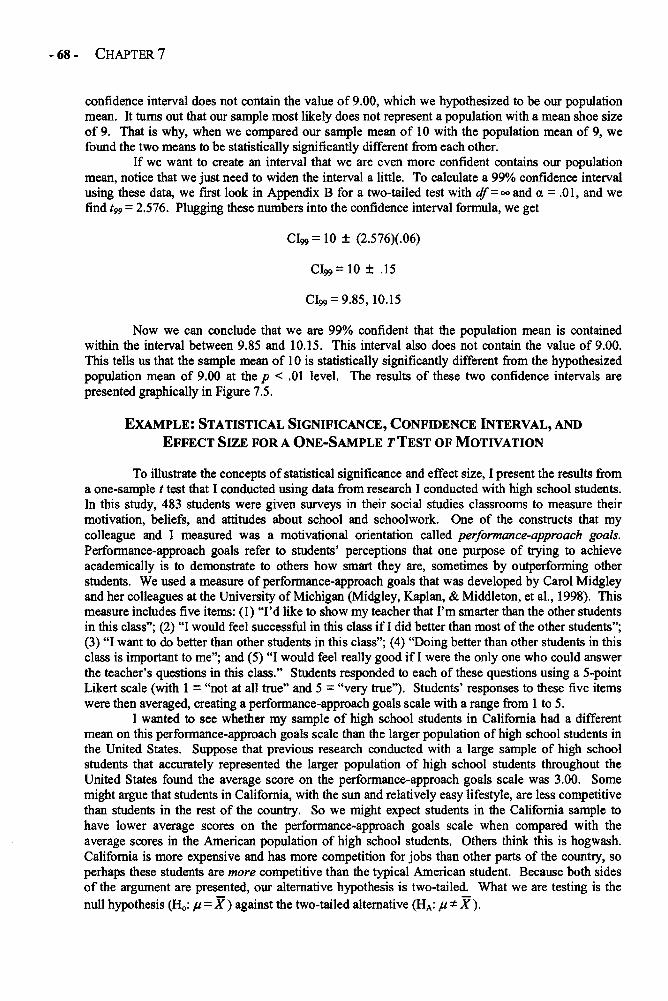
- 68 - CHAPTER 7
confidence interval does not contain the value of 9.00, which we hypothesized to be our populationmean. It turns out that our sample most likely does not represent a population with a mean shoe sizeof 9. That is why, when we compared our sample mean of 10 with the population mean of 9, wefound the two means to be statistically significantly different from each other.
If we want to create an interval that we are even more confident contains our populationmean, notice that we just need to widen the interval a little. To calculate a 99% confidence intervalusing these data, we first look in Appendix B for a two-tailed test with df=°° and a = .01, and wefind t99 = 2.576. Plugging these numbers into the confidence interval formula, we get
CI99 = 10 ± (2.576)(.06)
Cl99=10 ± .15
CLw = 9.85,10.15
Now we can conclude that we are 99% confident that the population mean is containedwithin the interval between 9.85 and 10.15. This interval also does not contain the value of 9.00.This tells us that the sample mean of 10 is statistically significantly different from the hypothesizedpopulation mean of 9.00 at the p < .01 level. The results of these two confidence intervals arepresented graphically in Figure 7.5.
EXAMPLE: STATISTICAL SIGNIFICANCE, CONFIDENCE INTERVAL, ANDEFFECT SIZE FOR A ONE-SAMPLE TTEST OF MOTIVATION
To illustrate the concepts of statistical significance and effect size, I present the results froma one-sample t test that I conducted using data from research I conducted with high school students.In this study, 483 students were given surveys in their social studies classrooms to measure theirmotivation, beliefs, and attitudes about school and schoolwork. One of the constructs that mycolleague and I measured was a motivational orientation called performance-approach goals.Performance-approach goals refer to students' perceptions that one purpose of trying to achieveacademically is to demonstrate to others how smart they are, sometimes by outperforming otherstudents. We used a measure of performance-approach goals that was developed by Carol Midgleyand her colleagues at the University of Michigan (Midgley, Kaplan, & Middleton, et al, 1998). Thismeasure includes five items: (1) "I'd like to show my teacher that I'm smarter than the other studentsin this class"; (2) "I would feel successful in this class if I did better than most of the other students";(3) "I want to do better than other students in this class"; (4) "Doing better than other students in thisclass is important to me"; and (5) "I would feel really good if I were the only one who could answerthe teacher's questions in this class." Students responded to each of these questions using a 5-pointLikert scale (with 1 = "not at all true" and 5 = "very true"). Students' responses to these five itemswere then averaged, creating a performance-approach goals scale with a range from 1 to 5.
I wanted to see whether my sample of high school students in California had a differentmean on this performance-approach goals scale than the larger population of high school students inthe United States. Suppose that previous research conducted with a large sample of high schoolstudents that accurately represented the larger population of high school students throughout theUnited States found the average score on the performance-approach goals scale was 3.00. Somemight argue that students in California, with the sun and relatively easy lifestyle, are less competitivethan students in the rest of the country. So we might expect students in the California sample tohave lower average scores on the performance-approach goals scale when compared with theaverage scores in the American population of high school students. Others think this is hogwash.California is more expensive and has more competition for jobs than other parts of the country, soperhaps these students are more competitive than the typical American student. Because both sidesof the argument are presented, our alternative hypothesis is two-tailed. What we are testing is thenull hypothesis (H0: u
= X) against the two-tailed alternative (HA: u = X ) .
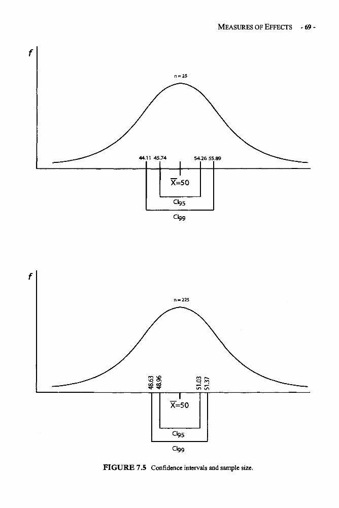
MEASURES OF EFFECTS - 69 -
FIGURE 7.5 Confidence intervals and sample size.
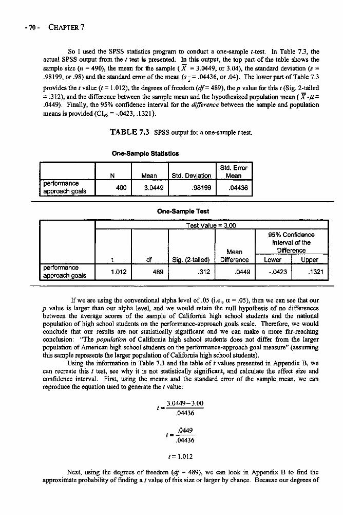
- 70 - CHAPTER 7
So I used the SPSS statistics program to conduct a one-sample Mest. In Table 7.3, theactual SPSS output from the t test is presented. In this output, the top part of the table shows thesample size (n = 490), the mean for the sample (X = 3.0449, or 3.04), the standard deviation (5- =.98199, or .98) and the standard error of the mean (s- - .04436, or .04). The lower part of Table 7.3
provides the t value (t - 1.012), the degrees of freedom ( d f = 489), the p value for this t (Sig. 2-tailed= .312), and the difference between the sample mean and the hypothesized population mean ( X -u =.0449). Finally, the 95% confidence interval for the difference between the sample and populationmeans is provided (CI95 = -.0423, .1321).
TABLE 7.3 SPSS output for a one-sample t test.
One-Sample Statistics
performanceapproach goals
N
490
Mean
3.0449
Std. Deviation
.98199
Std. ErrorMean
.04436
One-Sample Test
performanceapproach goals
Test Value = 3.00
t
1.012
df
489
Sig. (2-tailed)
.312
MeanDifference
.0449
95% ConfidenceInterval of the
DifferenceLower
-.0423
Upper
.1321
If we are using the conventional alpha level of .05 (i.e., a = .05), then we can see that ourp value is larger than our alpha level, and we would retain the null hypothesis of no differencesbetween the average scores of the sample of California high school students and the nationalpopulation of high school students on the performance-approach goals scale. Therefore, we wouldconclude that our results are not statistically significant and we can make a more far-reachingconclusion: "The population of California high school students does not differ from the largerpopulation of American high school students on the performance-approach goal measure" (assumingthis sample represents the larger population of California high school students).
Using the information in Table 7.3 and the table of t values presented in Appendix B, wecan recreate this t test, see why it is not statistically significant, and calculate the effect size andconfidence interval. First, using the means and the standard error of the sample mean, we canreproduce the equation used to generate the t value:
Next, using the degrees of freedom (df - 489), we can look in Appendix B to find theapproximate probability of finding a t value of this size or larger by chance. Because our degrees of
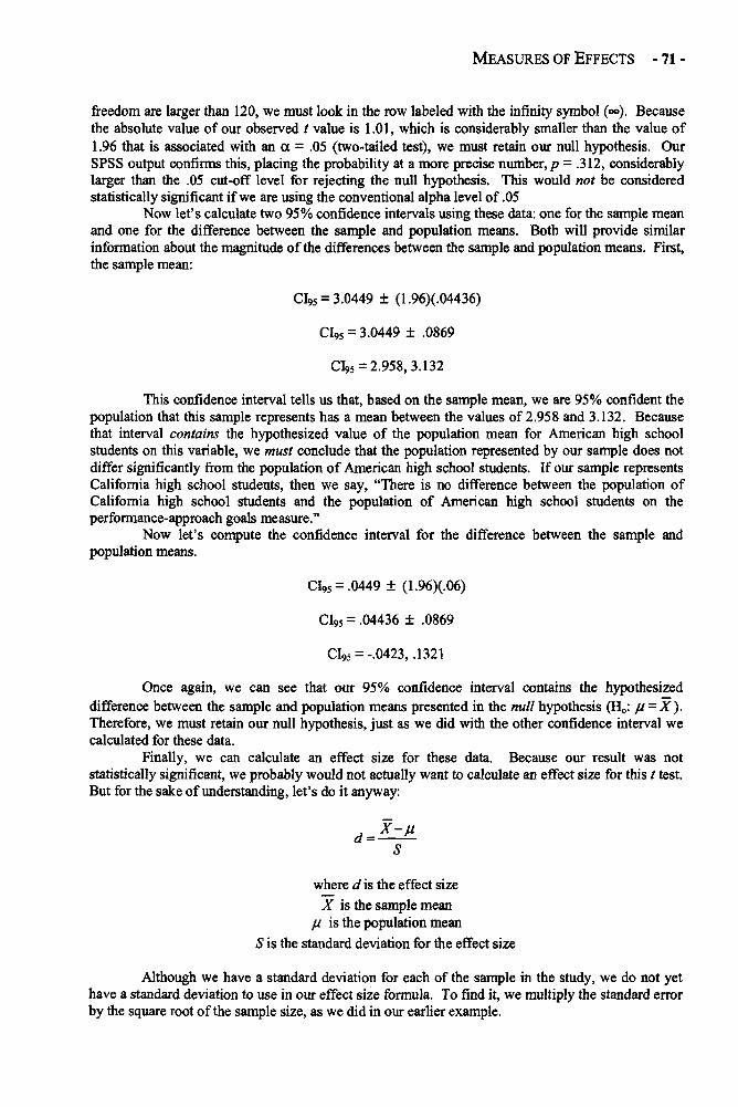
MEASURES OF EFFECTS - 71 -
freedom are larger than 120, we must look in the row labeled with the infinity symbol («»). Becausethe absolute value of our observed t value is 1.01, which is considerably smaller than the value of1.96 that is associated with an a = .05 (two-tailed test), we must retain our null hypothesis. OurSPSS output confirms this, placing the probability at a more precise number, p = .312, considerablylarger than the .05 cut-off level for rejecting the null hypothesis. This would not be consideredstatistically significant if we are using the conventional alpha level of .05
Now let's calculate two 95% confidence intervals using these data: one for the sample meanand one for the difference between the sample and population means. Both will provide similarinformation about the magnitude of the differences between the sample and population means. First,the sample mean:
CI95 = 3.0449 ± (1.96)(.04436)
CI95 = 3.0449 ± .0869
CI95 = 2.958,3.132
This confidence interval tells us that, based on the sample mean, we are 95% confident thepopulation that this sample represents has a mean between the values of 2.958 and 3.132. Becausethat interval contains the hypothesized value of the population mean for American high schoolstudents on this variable, we must conclude that the population represented by our sample does notdiffer significantly from the population of American high school students. If our sample representsCalifornia high school students, then we say, "There is no difference between the population ofCalifornia high school students and the population of American high school students on theperformance-approach goals measure."
Now let's compute the confidence interval for the difference between the sample andpopulation means.
CI95 = .0449± (1.96)(.06)
CI95 = .04436 ± .0869
CI95 = -.0423, .1321
Once again, we can see that our 95% confidence interval contains the hypothesizeddifference between the sample and population means presented in the null hypothesis (H0: u= X).Therefore, we must retain our null hypothesis, just as we did with the other confidence interval wecalculated for these data.
Finally, we can calculate an effect size for these data. Because our result was notstatistically significant, we probably would not actually want to calculate an effect size for this t test.But for the sake of understanding, let's do it anyway:
where d is the effect size
X is the sample meanu. is the population mean
S is the standard deviation for the effect size
Although we have a standard deviation for each of the sample in the study, we do not yethave a standard deviation to use in our effect size formula. To find it, we multiply the standard errorby the square root of the sample size, as we did in our earlier example.
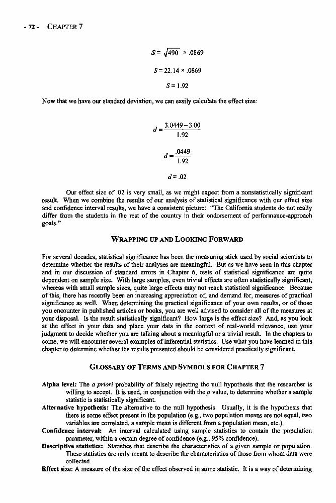
- 72 - CHAPTER 7
S= ^490" x.0869
S= 22.14 x.0869
S=1.92
Now that we have our standard deviation, we can easily calculate the effect size:
Our effect size of .02 is very small, as we might expect from a nonstatistically significantresult. When we combine the results of our analysis of statistical significance with our effect sizeand confidence interval results, we have a consistent picture: "The California students do not reallydiffer from the students in the rest of the country in their endorsement of performance-approachgoals."
WRAPPING UP AND LOOKING FORWARD
For several decades, statistical significance has been the measuring stick used by social scientists todetermine whether the results of their analyses are meaningful. But as we have seen in this chapterand in our discussion of standard errors in Chapter 6, tests of statistical significance are quitedependent on sample size. With large samples, even trivial effects are often statistically significant,whereas with small sample sizes, quite large effects may not reach statistical significance. Becauseof this, there has recently been an increasing appreciation of, and demand for, measures of practicalsignificance as well. When determining the practical significance of your own results, or of thoseyou encounter in published articles or books, you are well advised to consider all of the measures atyour disposal. Is the result statistically significant? How large is the effect size? And, as you lookat the effect in your data and place your data in the context of real-world relevance, use yourjudgment to decide whether you are talking about a meaningful or a trivial result. In the chapters tocome, we will encounter several examples of inferential statistics. Use what you have learned in thischapter to determine whether the results presented should be considered practically significant.
GLOSSARY OF TERMS AND SYMBOLS FOR CHAPTER 7
Alpha level: The a priori probability of falsely rejecting the null hypothesis that the researcher iswilling to accept. It is used, in conjunction with the p value, to determine whether a samplestatistic is statistically significant.
Alternative hypothesis: The alternative to the null hypothesis. Usually, it is the hypothesis thatthere is some effect present in the population (e.g., two population means are not equal, twovariables are correlated, a sample mean is different from a population mean, etc.).
Confidence interval: An interval calculated using sample statistics to contain the populationparameter, within a certain degree of confidence (e.g., 95% confidence).
Descriptive statistics: Statistics that describe the characteristics of a given sample or population.These statistics are only meant to describe the characteristics of those from whom data werecollected.
Effect size: A measure of the size of the effect observed in some statistic. It is a way of determining
MEASURES OF EFFECTS - 73 -
the practical significance of a statistic by reducing the impact of sample size.Inferential statistics: Statistics generated from sample data that are used to make inferences about
the characteristics of the population the sample is alleged to represent.Null hypothesis: The hypothesis that there is no effect in the population (e.g., that two population
means are not different from each other, that two variables are not correlated in thepopulation).
One-tailed: A test of statistical significance that is conducted just for one tail of the distribution(e.g., that the sample mean will be larger than the population mean).
Population: The group from which data are collected or a sample is selected. The populationencompasses the entire group for which the data are alleged to apply.
Practical significance: A judgment about whether a statistic is relevant, or of any importance, in thereal world.
p value: The probability of obtaining a statistic of a given size from a sample of a given size bychance, or due to random error.
Random chance: The probability of a statistical event occurring due simply to random variations inthe characteristics of samples of a given size selected randomly from a population.
Random sampling error: The error, or variation, associated with randomly selecting samples of agiven size from a population.
Sample: An individual or group, selected from a population, from whom or which data arecollected.
Statistical significance: When the probability of obtaining a statistic of a given size due strictly torandom sampling error, or chance, is less than the selected alpha level, the result is said tobe statistically significant. It also represents a rejection of the null hypothesis.
Two-tailed: A test of statistical significance that is conducted just for both tails of the distribution(e.g., that the sample mean will be different from the population mean).
Type I error: Rejecting the null hypothesis when in fact the null hypothesis is true.
p The p value, or probability.a The alpha level.d One measure of effect size.S The standard deviation used in the effect size formula.00 Infinity.sx The standard error calculated with the sample standard deviation.01 The standard error calculated with the population standard deviation.HO The null hypothesis.HA or HI The alternative hypothesis.
REFERENCES
Midgley, C., Kaplan, A., Middleton, M., et al. (1998). The development and validation of scalesassessing students' achievement goal orientations. Contemporary Educational Psychology, 23, 113-131.

This page intentionally left blank
CHAPTER 8
CORRELATION
In several of the previous chapters, we examined statistics and parameters that describe a singlevariable at a time, such as the mean, standard deviation, z scores, and standard errors. Although suchsingle-variable statistics are important, researchers are often interested in examining the relationsamong two or more variables. One of the most basic measures of the association among variables,and a foundational statistic for several more complex statistics, is the correlation coefficientAlthough there are a number of different types of correlation coefficients, the most commonly usedin social science research is the Pearson product-moment correlation coefficient. Most of thischapter is devoted to understanding this statistic, with a brief description of three other types ofcorrelations: the point-biserial coefficient, the Spearman rho coefficient, and the phi coefficient
When to Use Correlation and What It Tells Us
Researchers compute correlation coefficients when they want to know how two variables are relatedto each other. For a Pearson product-moment correlation, both of the variables must be measured onan interval or ratio scale and are known as continuous variables. For example, suppose I want toknow whether there is a relationship between the amount of time students spend studying for anexam and their scores on the exam. I suspect that the more hours students spend studying, the highertheir scores will be on the exam. But I also suspect that there is not a perfect correspondencebetween time spent studying and test scores. Some students will probably get low scores on theexam even if they study for a long time, simply because they may have a hard time understandingthe material. Indeed, there will probably be a number of students who spend an inordinately longperiod of time studying for the test precisely because they are having trouble understanding thematerial. On the other hand, there will probably be some students who do very well on the testwithout spending very much time studying. Despite these "exceptions" to my rule, I stillhypothesize that, on average, as the amount of time spent studying increases, so do students' scoreson the exam.
There are two fundamental characteristics of correlation coefficients researchers care about.The first of these is the direction of the correlation coefficient. Correlation coefficients can beeither positive or negative. A positive correlation indicates that the values on the two variablesbeing analyzed move in the same direction. That is, as scores on one variable go up, scores on theother variable go up as well (on average). Similarly, on average, as scores on one variable go down,scores on the other variable go down. Returning to my earlier example, if there is a positivecorrelation between the amount of time students spend studying and their test scores, I can tell that,on average, the more time students spend studying, the higher their scores are on the test. This isequivalent to saying that, on average, the less time they spend studying, the lower their scores are onthe test. Both of these represent a positive correlation between time spent studying and test scores.(Note: I keep saying "on average" because it is important to note that the presence of a correlationbetween two variables does not mean that this relationship holds true for each member of the sampleor population. Rather, it means that, in general, there is a relationship of a given direction andstrength between two variables in the sample or population.)
A negative correlation indicates that the values on the two variables being analyzed movein opposite directions. That is, as scores on one variable go up, scores on the other variable godown, and vice versa (on average). If there were a negative correlation between the amount of timespent studying and test scores, I would know that, on average, the more time students spend studying
-75-
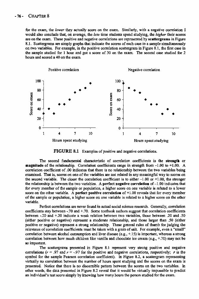
- 76 - CHAPTER 8
for the exam, the lower they actually score on the exam. Similarly, with a negative correlation Iwould also conclude that, on average, the less time students spend studying, the higher their scoresare on the exam. These positive and negative correlations are represented by scattergrams in Figure8.1. Scattergrams are simply graphs that indicate the scores of each case in a sample simultaneouslyon two variables. For example, in the positive correlation scattergram in Figure 8.1, the first case inthe sample studied for 1 hour and got a score of 30 on the exam. The second case studied for 2hours and scored a 40 on the exam.
FIGURE 8.1 Examples of positive and negative correlations.
The second fundamental characteristic of correlation coefficients is the strength ormagnitude of the relationship. Correlation coefficients range in strength from -1.00 to +1.00. Acorrelation coefficient of .00 indicates that there is no relationship between the two variables beingexamined. That is, scores on one of the variables are not related in any meaningful way to scores onthe second variable. The closer the correlation coefficient is to either -1.00 or +1.00, the strongerthe relationship is between the two variables. A perfect negative correlation of-1.00 indicates thatfor every member of the sample or population, a higher score on one variable is related to a lowerscore on the other variable. A perfect positive correlation of +1.00 reveals that for every memberof the sample or population, a higher score on one variable is related to a higher score on the othervariable.
Perfect correlations are never found in actual social science research. Generally, correlationcoefficients stay between -.70 and +.70. Some textbook authors suggest that correlation coefficientsbetween -.20 and +.20 indicate a weak relation between two variables, those between .20 and .50(either positive or negative) represent a moderate relationship, and those larger than .50 (eitherpositive or negative) represent a strong relationship. These general rules of thumb for judging therelevance of correlation coefficients must be taken with a grain of salt. For example, even a "small"correlation between alcohol consumption and liver disease (e.g., +.15) is important, whereas a strongcorrelation between how much children like vanilla and chocolate ice cream (e.g., +.70) may not beso important.
The scattergrams presented in Figure 8.1 represent very strong positive and negativecorrelations (r = .97 and r = -.97 for the positive and negative correlations, respectively; r is thesymbol for the sample Pearson correlation coefficient). In Figure 8.2, a scattergram representingvirtually no correlation between the number of hours spent studying and the scores on the exam ispresented. Notice that there is no discernible pattern between the scores on the two variables. Inother words, the data presented in Figure 8.2 reveal that it would be virtually impossible to predictan individual's test score simply by knowing how many hours the person studied for the exam.

CORRELATION - 77 -
FIGURE 8.2 No correlation between hours spent studying and exam scores.
PEARSON CORRELATION COEFFICIENTS IN DEPTH
The first step in understanding how Pearson correlation coefficients are calculated is to notice thatwe are concerned with a sample's scores on two variables at the same time. Returning to ourprevious example of study time and test scores, suppose that we randomly select a sample of fivestudents and measure the time they spent studying for the exam and their exam scores. The data arepresented in Table 8.1 (with a scattergram in Figure 8.3).
TABLE 8.1 Data for correlation coefficient.
Hours Spent Studying(X Variable)
Student 1
Student 2
Student 3
Student 4
Student 5
5
6
7
8
9
Exam Score(Y Variable)
80
85
70
90
85
For these data to be used in a correlation analysis, it is critical that the scores on the twovariables are paired. That is, for each student in my sample, the score on the x variable (hours spentstudying) is paired with his or her own score on the 7 variable (exam score). If I want to determinethe relation between hours spent studying and exam scores, I cannot pair Student 1's hours spentstudying with Student 4's test score. I must match each student's score on the X variable with his or
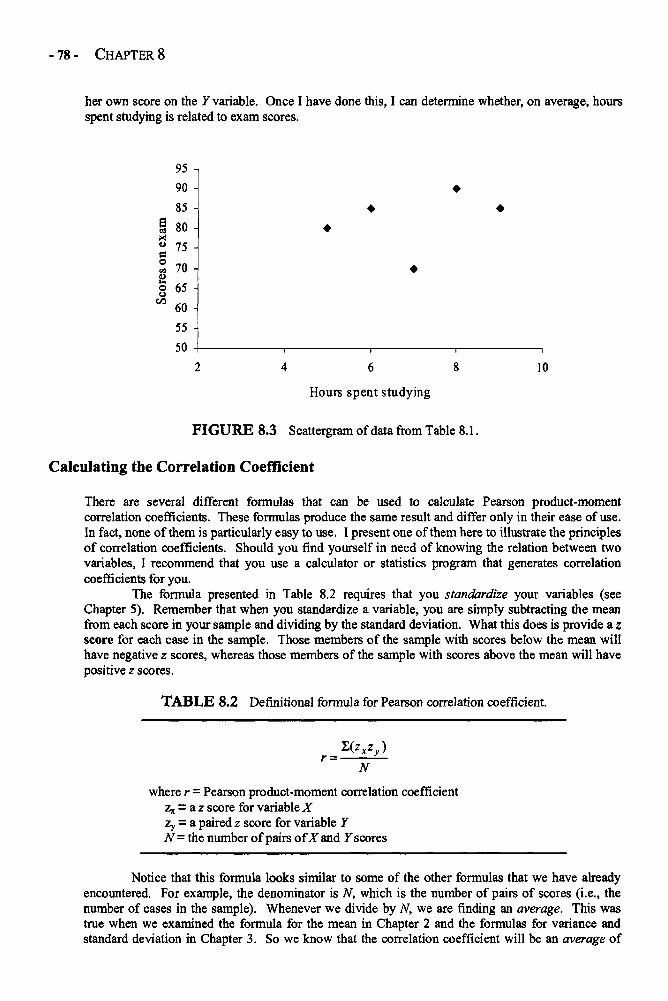
- 78 - CHAPTER 8
her own score on the Y variable. Once I have done this, I can determine whether, on average, hoursspent studying is related to exam scores.
FIGURE 8.3 Scattergram of data from Table 8.1.
Calculating the Correlation Coefficient
There are several different formulas that can be used to calculate Pearson product-momentcorrelation coefficients. These formulas produce the same result and differ only in their ease of use.In fact, none of them is particularly easy to use. I present one of them here to illustrate the principlesof correlation coefficients. Should you find yourself in need of knowing the relation between twovariables, I recommend that you use a calculator or statistics program that generates correlationcoefficients for you.
The formula presented in Table 8.2 requires that you standardize your variables (seeChapter 5). Remember that when you standardize a variable, you are simply subtracting the meanfrom each score in your sample and dividing by the standard deviation. What this does is provide a zscore for each case in the sample. Those members of the sample with scores below the mean willhave negative z scores, whereas those members of the sample with scores above the mean will havepositive 2 scores.
TABLE 8.2 Definitional formula for Pearson correlation coefficient.
where r - Pearson product-moment correlation coefficientZx = a z score for variable XZy = a paired z score for variable YN = the number of pairs of X and Y scores
Notice that this formula looks similar to some of the other formulas that we have alreadyencountered. For example, the denominator is N, which is the number of pairs of scores (i.e., thenumber of cases in the sample). Whenever we divide by N, we are finding an average. This wastrue when we examined the formula for the mean in Chapter 2 and the formulas for variance andstandard deviation in Chapter 3. So we know that the correlation coefficient will be an average of
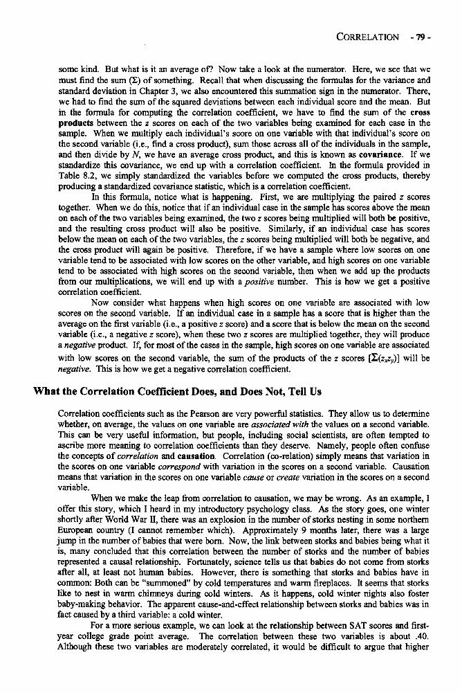
CORRELATION - 79 -
some kind. But what is it an average of? Now take a look at the numerator. Here, we see that wemust find the sum (E) of something. Recall that when discussing the formulas for the variance andstandard deviation in Chapter 3, we also encountered this summation sign in the numerator. There,we had to find the sum of the squared deviations between each individual score and the mean. Butin the formula for computing the correlation coefficient, we have to find the sum of the crossproducts between the z scores on each of the two variables being examined for each case in thesample. When we multiply each individual's score on one variable with that individual's score onthe second variable (i.e., find a cross product), sum those across all of the individuals in the sample,and then divide by N, we have an average cross product, and this is known as covariance. If westandardize this covariance, we end up with a correlation coefficient. In the formula provided inTable 8.2, we simply standardized the variables before we computed the cross products, therebyproducing a standardized covariance statistic, which is a correlation coefficient.
In this formula, notice what is happening. First, we are multiplying the paired z scorestogether. When we do this, notice that if an individual case in the sample has scores above the meanon each of the two variables being examined, the two z scores being multiplied will both be positive,and the resulting cross product will also be positive. Similarly, if an individual case has scoresbelow the mean on each of the two variables, the z scores being multiplied will both be negative, andthe cross product will again be positive. Therefore, if we have a sample where low scores on onevariable tend to be associated with low scores on the other variable, and high scores on one variabletend to be associated with high scores on the second variable, then when we add up the productsfrom our multiplications, we will end up with a positive number. This is how we get a positivecorrelation coefficient.
Now consider what happens when high scores on one variable are associated with lowscores on the second variable. If an individual case in a sample has a score that is higher than theaverage on the first variable (i.e., a positive z score) and a score that is below the mean on the secondvariable (i.e., a negative z score), when these two z scores are multiplied together, they will producea negative product. If, for most of the cases in the sample, high scores on one variable are associated
with low scores on the second variable, the sum of the products of the z scores [E(zxzy)] will benegative. This is how we get a negative correlation coefficient.
What the Correlation Coefficient Does, and Does Not, Tell Us
Correlation coefficients such as the Pearson are very powerful statistics. They allow us to determinewhether, on average, the values on one variable are associated with the values on a second variable.This can be very useful information, but people, including social scientists, are often tempted toascribe more meaning to correlation coefficients than they deserve. Namely, people often confusethe concepts of correlation and causation. Correlation (co-relation) simply means that variation inthe scores on one variable correspond with variation in the scores on a second variable. Causationmeans that variation in the scores on one variable cause or create variation in the scores on a secondvariable.
When we make the leap from correlation to causation, we may be wrong. As an example, Ioffer this story, which I heard in my introductory psychology class. As the story goes, one wintershortly after World War II, there was an explosion in the number of storks nesting in some northernEuropean country (I cannot remember which). Approximately 9 months later, there was a largejump in the number of babies that were born. Now, the link between storks and babies being what itis, many concluded that this correlation between the number of storks and the number of babiesrepresented a causal relationship. Fortunately, science tells us that babies do not come from storksafter all, at least not human babies. However, there is something that storks and babies have incommon: Both can be "summoned" by cold temperatures and warm fireplaces. It seems that storkslike to nest in warm chimneys during cold winters. As it happens, cold winter nights also fosterbaby-making behavior. The apparent cause-and-effect relationship between storks and babies was infact caused by a third variable: a cold winter.
For a more serious example, we can look at the relationship between SAT scores and first-year college grade point average. The correlation between these two variables is about .40.Although these two variables are moderately correlated, it would be difficult to argue that higher
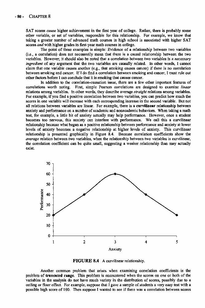
- 80 - CHAPTER 8
SAT scores cause higher achievement in the first year of college. Rather, there is probably someother variable, or set of variables, responsible for this relationship. For example, we know thattaking a greater number of advanced math courses in high school is associated with higher SATscores and with higher grades in first-year math courses in college.
The point of these examples is simple: Evidence of a relationship between two variables(i.e., a correlation) does not necessarily mean that there is a causal relationship between the twovariables. However, it should also be noted that a correlation between two variables is a necessaryingredient of any argument that the two variables are causally related. In other words, I cannotclaim that one variable causes another (e.g., that smoking causes cancer) if there is no correlationbetween smoking and cancer. If I do find a correlation between smoking and cancer, I must rule outother factors before I can conclude that it is smoking that causes cancer.
In addition to the correlation-causation issue, there are a few other important features ofcorrelations worth noting. First, simple Pearson correlations are designed to examine linearrelations among variables. In other words, they describe average straight relations among variables.For example, if you find a positive correlation between two variables, you can predict how much thescores in one variable will increase with each corresponding increase in the second variable. But notall relations between variables are linear. For example, there is a curvilinear relationship betweenanxiety and performance on a number of academic and nonacademic behaviors. When taking a mathtest, for example, a little bit of anxiety actually may help performance. However, once a studentbecomes too nervous, this anxiety can interfere with performance. We call this a curvilinearrelationship because what began as a positive relationship between performance and anxiety at lowerlevels of anxiety becomes a negative relationship at higher levels of anxiety. This curvilinearrelationship is presented graphically in Figure 8.4. Because correlation coefficients show theaverage relation between two variables, when the relationship between two variables is curvilinear,the correlation coefficient can be quite small, suggesting a weaker relationship than may actuallyexist.
FIGURE 8.4 A curvilinear relationship.
Another common problem that arises when examining correlation coefficients is theproblem of truncated range. This problem is encountered when the scores on one or both of thevariables in the analysis do not have much variety in the distribution of scores, possibly due to aceiling or floor effect. For example, suppose that I gave a sample of students a very easy test with apossible high score of 100. Then suppose I wanted to see if there was a correlation between scores
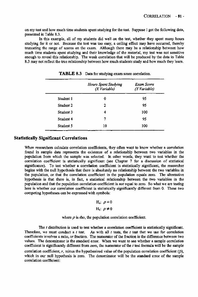
CORRELATION - 81 -
on my test and how much time students spent studying for the test. Suppose I got the following data,presented in Table 8.3.
In this example, all of my students did well on the test, whether they spent many hoursstudying for it or not. Because the test was too easy, a ceiling effect may have occurred, therebytruncating the range of scores on the exam. Although there may be a relationship between howmuch time students spent studying and their knowledge of the material, my test was not sensitiveenough to reveal this relationship. The weak correlation that will be produced by the data in Table8.3 may not reflect the true relationship between how much students study and how much they learn.
TABLE 8.3 Data for studying-exam score correlation.
Hours Spent Studying(X Variable)
Student 1
Student 2
Student 3
Student 4
Student 5
0
2
4
7
10
Exam Score(Y Variable)
95
95
100
95
100
Statistically Significant Correlations
When researchers calculate correlation coefficients, they often want to know whether a correlationfound in sample data represents the existence of a relationship between two variables in thepopulation from which the sample was selected. In other words, they want to test whether thecorrelation coefficient is statistically significant (see Chapter 7 for a discussion of statisticalsignificance). To test whether a correlation coefficient is statistically significant, the researcherbegins with the null hypothesis that there is absolutely no relationship between the two variables inthe population, or that the correlation coefficient in the population equals zero. The alternativehypothesis is that there is, in fact, a statistical relationship between the two variables in thepopulation and that the population correlation coefficient is not equal to zero. So what we are testinghere is whether our correlation coefficient is statistically significantly different from 0. These twocompeting hypotheses can be expressed with symbols:
where p is rho, the population correlation coefficient.
The t distribution is used to test whether a correlation coefficient is statistically significant.Therefore, we must conduct a t test. As with all t tests, the t test that we use for correlationcoefficients involves a ratio, or fraction. The numerator of the fraction is the difference between twovalues. The denominator is the standard error. When we want to see whether a sample correlationcoefficient is significantly different from zero, the numerator of the t test formula will be the sample
correlation coefficient, r, minus the hypothesized value of the population correlation coefficient (p),which in our null hypothesis is zero. The denominator will be the standard error of the samplecorrelation coefficient:
- 82 - CHAPTER 8
where r is the sample correlation coefficient,p is the population correlation coefficient,
sr is the standard error of the sample correlation coefficient.
Fortunately, with the help of a little algebra, we do not need to calculate sr to calculate the t
value for correlation coefficients. First, for the sake of knowledge, let me present the formula for sr:
s r =J(1 - r 2 )+(N-2)
where r2 is the correlation coefficient squared andN is the number of cases in the sample.
The formula for calculating the t value is
where degrees of freedom is the number of cases in the sample minus two (df=N- 2)
To illustrate this formula in action, let's consider an example. Some research suggests thatthere is a relationship between the number of hours of sunlight people are exposed to during the dayand their mood. People living at extreme northern latitudes, for example, are exposed to very littlesunlight in the depths of winter days and weeks without more than a few hours of sunlight per day.There is some evidence that such sunlight deprivation is related to feelings of depression andsadness. In fact, there is even a name for the condition: seasonal affective disorder, or SAD. Toexamine this relationship for myself, I randomly select 100 people from various regions of theworld, measure the time from sunrise to sunset on a given day where each person lives, and get ameasure of each person's mood on a scale from 1 to 10 (1 = "very sad," 10 = "very happy").Because the members of my sample live at various latitudes, the number of daylight hours will vary.If I conduct my study in January, those participants living in the north will have relatively shortdays, whereas those living in the south will have long days.
Suppose that I compute a Pearson correlation coefficient with these data and find that thecorrelation between number of sunlight hours in the day and scores on the mood scale is r = .25. Isthis a statistically significant correlation? To answer that question, we must find a t value associatedwith this correlation coefficient and determine the probability of obtaining a t value of this size bychance (see Chapter 7). In this example,
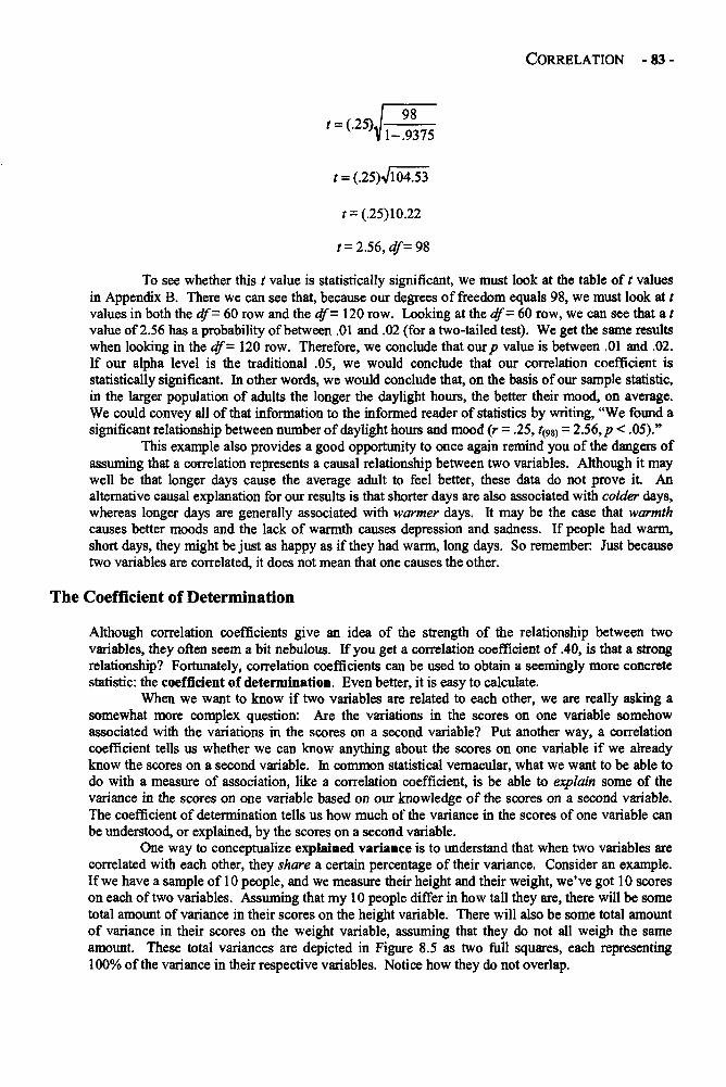
CORRELATION - 83 -
To see whether this t value is statistically significant, we must look at the table of t valuesin Appendix B. There we can see that, because our degrees of freedom equals 98, we must look at tvalues in both the df- 60 row and the df- 120 row. Looking at the df = 60 row, we can see that a tvalue of 2.56 has a probability of between .01 and .02 (for a two-tailed test). We get the same resultswhen looking in the df = 120 row. Therefore, we conclude that our p value is between .01 and .02.If our alpha level is the traditional .05, we would conclude that our correlation coefficient isstatistically significant. In other words, we would conclude that, on the basis of our sample statistic,in the larger population of adults the longer the daylight hours, the better their mood, on average.We could convey all of that information to the informed reader of statistics by writing, "We found asignificant relationship between number of daylight hours and mood (r = .25, t(98) = 2.56, p < .05)."
This example also provides a good opportunity to once again remind you of the dangers ofassuming that a correlation represents a causal relationship between two variables. Although it maywell be that longer days cause the average adult to feel better, these data do not prove it. Analternative causal explanation for our results is that shorter days are also associated with colder days,whereas longer days are generally associated with warmer days. It may be the case that warmthcauses better moods and the lack of warmth causes depression and sadness. If people had warm,short days, they might be just as happy as if they had warm, long days. So remember: Just becausetwo variables are correlated, it does not mean that one causes the other.
The Coefficient of Determination
Although correlation coefficients give an idea of the strength of the relationship between twovariables, they often seem a bit nebulous. If you get a correlation coefficient of .40, is that a strongrelationship? Fortunately, correlation coefficients can be used to obtain a seemingly more concretestatistic: the coefficient of determination. Even better, it is easy to calculate.
When we want to know if two variables are related to each other, we are really asking asomewhat more complex question: Are the variations in the scores on one variable somehowassociated with the variations in the scores on a second variable? Put another way, a correlationcoefficient tells us whether we can know anything about the scores on one variable if we alreadyknow the scores on a second variable. In common statistical vernacular, what we want to be able todo with a measure of association, like a correlation coefficient, is be able to explain some of thevariance in the scores on one variable based on our knowledge of the scores on a second variable.The coefficient of determination tells us how much of the variance in the scores of one variable canbe understood, or explained, by the scores on a second variable.
One way to conceptualize explained variance is to understand that when two variables arecorrelated with each other, they share a certain percentage of their variance. Consider an example.If we have a sample of 10 people, and we measure their height and their weight, we've got 10 scoreson each of two variables. Assuming that my 10 people differ in how tall they are, there will be sometotal amount of variance in their scores on the height variable. There will also be some total amountof variance in their scores on the weight variable, assuming that they do not all weigh the sameamount. These total variances are depicted in Figure 8.5 as two full squares, each representing100% of the variance in their respective variables. Notice how they do not overlap.
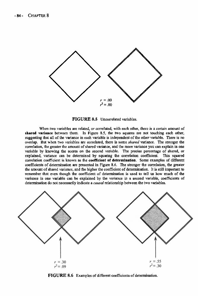
- 84 - CHAPTER 8
FIGURE 8.5 Uncorrelated variables.
When two variables are related, or correlated, with each other, there is a certain amount ofshared variance between them. In Figure 8.5, the two squares are not touching each other,suggesting that all of the variance in each variable is independent of the other variable. There is nooverlap. But when two variables are correlated, there is some shared variance. The stronger thecorrelation, the greater the amount of shared variance, and the more variance you can explain in onevariable by knowing the scores on the second variable. The precise percentage of shared, orexplained, variance can be determined by squaring the correlation coefficient. This squaredcorrelation coefficient is known as the coefficient of determination. Some examples of differentcoefficients of determination are presented in Figure 8.6. The stronger the correlation, the greaterthe amount of shared variance, and the higher the coefficient of determination. It is still important toremember that even though the coefficient of determination is used to tell us how much of thevariance in one variable can be explained by the variance in a second variable, coefficients ofdetermination do not necessarily indicate a causal relationship between the two variables.
FIGURE 8.6 Examples of different coefficients of determination.
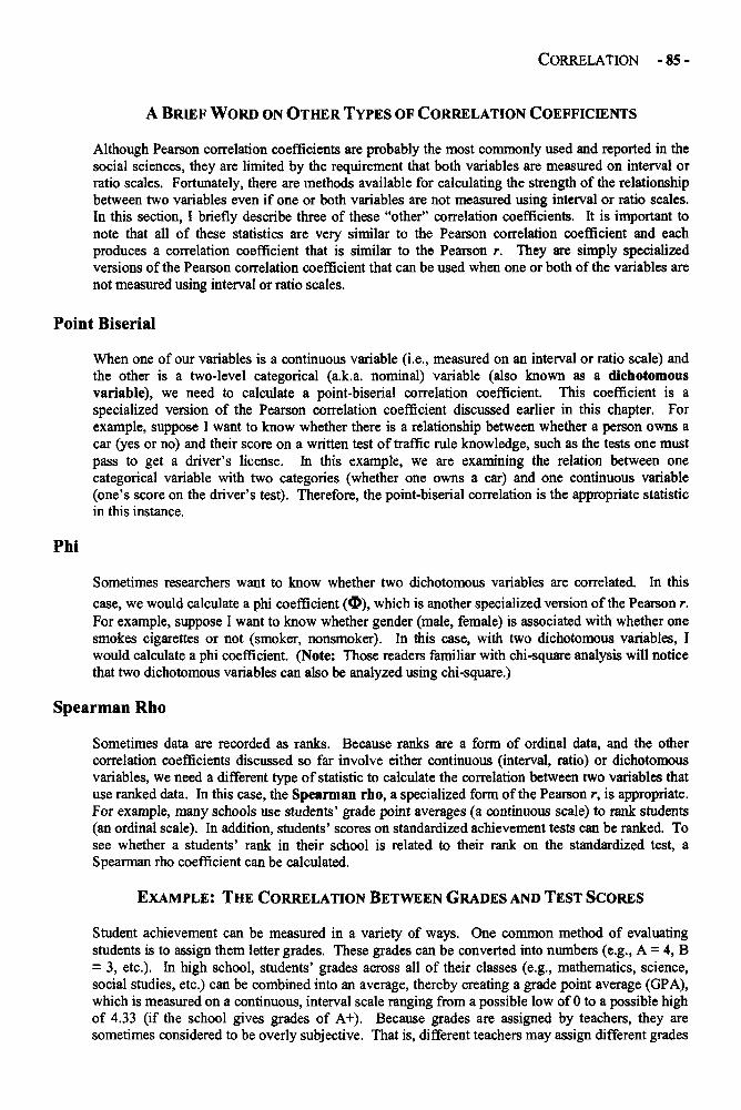
CORRELATION - 85 -
A BRIEF WORD ON OTHER TYPES OF CORRELATION COEFFICIENTS
Although Pearson correlation coefficients are probably the most commonly used and reported in thesocial sciences, they are limited by the requirement that both variables are measured on interval orratio scales. Fortunately, there are methods available for calculating the strength of the relationshipbetween two variables even if one or both variables are not measured using interval or ratio scales.In this section, I briefly describe three of these "other" correlation coefficients. It is important tonote that all of these statistics are very similar to the Pearson correlation coefficient and eachproduces a correlation coefficient that is similar to the Pearson r. They are simply specializedversions of the Pearson correlation coefficient that can be used when one or both of the variables arenot measured using interval or ratio scales.
Point Biserial
When one of our variables is a continuous variable (i.e., measured on an interval or ratio scale) andthe other is a two-level categorical (a.k.a. nominal) variable (also known as a dichotomousvariable), we need to calculate a point-biserial correlation coefficient. This coefficient is aspecialized version of the Pearson correlation coefficient discussed earlier in this chapter. Forexample, suppose I want to know whether there is a relationship between whether a person owns acar (yes or no) and their score on a written test of traffic rule knowledge, such as the tests one mustpass to get a driver's license. In this example, we are examining the relation between onecategorical variable with two categories (whether one owns a car) and one continuous variable(one's score on the driver's test). Therefore, the point-biserial correlation is the appropriate statisticin this instance.
Phi
Sometimes researchers want to know whether two dichotomous variables are correlated. In this
case, we would calculate a phi coefficient (O), which is another specialized version of the Pearson r.For example, suppose I want to know whether gender (male, female) is associated with whether onesmokes cigarettes or not (smoker, nonsmoker). In this case, with two dichotomous variables, Iwould calculate a phi coefficient. (Note: Those readers familiar with chi-square analysis will noticethat two dichotomous variables can also be analyzed using chi-square.)
Spearman Rho
Sometimes data are recorded as ranks. Because ranks are a form of ordinal data, and the othercorrelation coefficients discussed so far involve either continuous (interval, ratio) or dichotomousvariables, we need a different type of statistic to calculate the correlation between two variables thatuse ranked data. In this case, the Spearman rho, a specialized form of the Pearson r, is appropriate.For example, many schools use students' grade point averages (a continuous scale) to rank students(an ordinal scale). In addition, students' scores on standardized achievement tests can be ranked. Tosee whether a students' rank in their school is related to their rank on the standardized test, aSpearman rho coefficient can be calculated.
EXAMPLE: THE CORRELATION BETWEEN GRADES AND TEST SCORES
Student achievement can be measured in a variety of ways. One common method of evaluatingstudents is to assign them letter grades. These grades can be converted into numbers (e.g., A = 4, B= 3, etc.). In high school, students' grades across all of their classes (e.g., mathematics, science,social studies, etc.) can be combined into an average, thereby creating a grade point average (GPA),which is measured on a continuous, interval scale ranging from a possible low of 0 to a possible highof 4.33 (if the school gives grades of A+). Because grades are assigned by teachers, they aresometimes considered to be overly subjective. That is, different teachers may assign different grades

- 86 - CHAPTER 8
to the same work. Similarly, there are some individual teachers that may give different grades totwo students who produce the same quality of work. To ostensibly overcome such subjectivity,another form of assessment, the standardized test, was created. With this type of assessment, allstudents of a given grade level answer the same questions and their responses are scored bycomputer, thereby removing the human element and its subjectivity.
Some argue that standardized tests of ability and teacher-assigned grades generally measurethe same thing. That is, for the most part, bright students will score well both on the test and in theirgrades. Others argue that standardized tests of ability and teacher-assigned grades really measuresomewhat different things. Whereas standardized tests may measure how well students answermultiple-choice questions, teachers have the benefit of knowing students, and can take things likestudents' effort, creativity, and motivation into account when assigning grades. The first step indiscovering which of these two viewpoints is more accurate is to see how strongly grades and testscores are related to each other. If there is a very strong correlation between the two, then bothgrades and test scores may in fact be measuring the same general trait. But if the two scores are onlymoderately correlated, perhaps they really do measure separate constructs. By constructs, I mean theactual "thing" that we are trying to measure. In the preceding example, if grades and test scores arestrongly correlated, we could argue that both of these measures represent some underlying construct,such as "intelligence" or "academic ability." On the other hand, if these two variables are notstrongly correlated, they each may represent different things, or constructs.
My colleague, Carol Giancarlo, and I collected data from a sample of 314 eleventh-gradestudents at a high school in California. Among the data we collected were their cumulative GPAs(i.e., their GPAs accumulated from the time they began high school until the time the data werecollected). In addition, we gave students the Naglieri Nonverbal Ability Test (NNAT; Naglieri,1996), a nonverbal test of general mental reasoning and critical thinking skills. To see if there was astatistically significant correlation between these two measures of ability, I used the SPSS statisticalsoftware program to calculate a correlation coefficient and a p value. The SPSS printout from thisanalysis is presented in Table 8.5.
The results presented in Table 8.5 provide several pieces of information. First, there arethree correlation coefficients presented. The correlations on the diagonal show the correlationbetween a single variable and itself. Therefore, the first correlation coefficient presented reveals matGPA is correlated with itself perfectly (r = 1.0000). Because we always get a correlation of 1.00when we correlate a variable with itself, these correlations presented on the diagonal aremeaningless. That is why there is not a p value reported for them. The numbers in the parentheses,just below the correlation coefficients, report the sample size. There were 314 eleventh-gradestudents in this sample. The correlation coefficient that is off the diagonal is the one we're interestedin. Here, we can see that students' GPAs were moderately correlated with their scores on theNaglieri test (r = .4291). This correlation is statistically significant, with a p value of less than .0001(p < .0001).
TABLE 8.4 SPSS printout of correlation analysis.
GPA Naglieri
GPA
Naglieri
1(P
(P
.0000314)
— .
.4291314)
= .000
1.0000( 314)P = •
To gain a clearer understanding of the relationship between GPA and Naglieri test scores,we can calculate a coefficient of determination. We do this by squaring the correlation coefficient.When we square this correlation coefficient (.4291 x .4291 = .1841), we see that GPA explains a
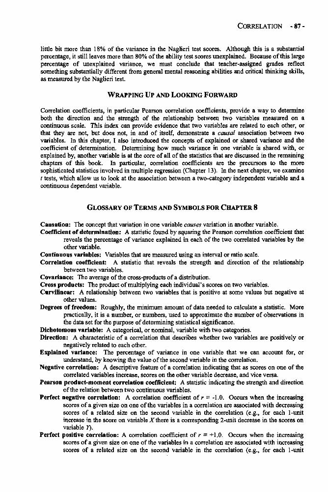
CORRELATION - 87 -
little bit more than 18% of the variance in the Naglieri test scores. Although this is a substantialpercentage, it still leaves more than 80% of the ability test scores unexplained. Because of this largepercentage of unexplained variance, we must conclude that teacher-assigned grades reflectsomething substantially different from general mental reasoning abilities and critical thinking skills,as measured by the Naglieri test.
WRAPPING UP AND LOOKING FORWARD
Correlation coefficients, in particular Pearson correlation coefficients, provide a way to determineboth the direction and the strength of the relationship between two variables measured on acontinuous scale. This index can provide evidence that two variables are related to each other, orthat they are not, but does not, in and of itself, demonstrate a causal association between twovariables. In this chapter, I also introduced the concepts of explained or shared variance and thecoefficient of determination. Determining how much variance in one variable is shared with, orexplained by, another variable is at the core of all of the statistics that are discussed in the remainingchapters of this book. In particular, correlation coefficients are the precursors to the moresophisticated statistics involved in multiple regression (Chapter 13). In the next chapter, we examinet tests, which allow us to look at the association between a two-category independent variable and acontinuous dependent variable.
GLOSSARY OF TERMS AND SYMBOLS FOR CHAPTER 8
Causation: The concept that variation in one variable causes variation in another variable.Coefficient of determination: A statistic found by squaring the Pearson correlation coefficient that
reveals the percentage of variance explained in each of the two correlated variables by theother variable.
Continuous variables: Variables that are measured using an interval or ratio scale.Correlation coefficient: A statistic that reveals the strength and direction of the relationship
between two variables.Covariance: The average of the cross-products of a distribution.Cross products: The product of multiplying each individual's scores on two variables.Curvilinear: A relationship between two variables that is positive at some values but negative at
other values.Degrees of freedom: Roughly, the minimum amount of data needed to calculate a statistic. More
practically, it is a number, or numbers, used to approximate the number of observations inthe data set for the purpose of determining statistical significance.
Dichotomous variable: A categorical, or nominal, variable with two categories.Direction: A characteristic of a correlation that describes whether two variables are positively or
negatively related to each other.Explained variance: The percentage of variance in one variable that we can account for, or
understand, by knowing the value of the second variable in the correlation.Negative correlation: A descriptive feature of a correlation indicating that as scores on one of the
correlated variables increase, scores on the other variable decrease, and vice versa.Pearson product-moment correlation coefficient: A statistic indicating the strength and direction
of the relation between two continuous variables.Perfect negative correlation: A correlation coefficient of r = -1.0. Occurs when the increasing
scores of a given size on one of the variables in a correlation are associated with decreasingscores of a related size on the second variable in the correlation (e.g., for each 1-unitincrease in the score on variable X there is a corresponding 2-unit decrease in the scores onvariable Y).
Perfect positive correlation: A correlation coefficient of r = +1.0. Occurs when the increasingscores of a given size on one of the variables in a correlation are associated with increasingscores of a related size on the second variable in the correlation (e.g., for each 1-unit
- 88 - CHAPTER 8
increase in the score on variable X there is a corresponding 2-unit increase in the scores onvariable Y).
Phi coefficient: The coefficient describing the correlation between two dichotomous variables.Point-biserial coefficient: The coefficient describing the relationship between one interval or ratio
scaled (i.e., continuous) variable and one dichotomous variable.Positive correlation: A characteristic of a correlation; when the scores on the two correlated
variables move in the same direction, on average. As the scores on one variable rise, scoreson the other variable rise, and vice versa.
Scattergram: A graphical depiction of each member of a distribution's score on two variablessimultaneously.
Shared variance: The concept of two variables overlapping such that some of the variance in eachvariable is shared. The stronger the correlation between two variables, the greater theamount of shared variance between them.
Spearman rho coefficient: The correlation coefficient used to measure the association between twovariables measured on an ordinal scale (e.g., ranked data).
Strength, magnitude: A characteristic of the correlation with a focus on how strongly twovariables are related.
Truncated range: When the responses on a variable are clustered near the top or the bottom of thepossible range of scores, thereby limiting the range of scores and possibly limiting thestrength of the correlation.
z score: Standardized score.
r The sample Pearson correlation coefficient.
p Rho, the population correlation coefficient.
sr The standard error of the correlation coefficient.
r2 The coefficient of determination.
df Degrees of freedom.
O The phi coefficient, which is the correlation between two dichotomous variables.
REFERENCES AND RECOMMENDED READING
Hinkle, D. E., Wiersma, W., & Jurs, S. G. (1998). Applied statistics for the behavioralsciences (4th ed.). Boston: Houghton Mifflin.
Naglieri, J.A. (1996). The Naglieri nonverbal ability test. San Antonio, TX: HarcourtBrace.
CHAPTER 9
t TESTS
What Is a t Test?
Because there is a distinction between the common statistical vernacular definition of t tests and themore technical definition, t tests can be a little confusing. The common-use definition or descriptionof t tests is simply comparing two means to see if they are significantly different from each other.The more technical definition or description of a t test is any statistical test that uses the t, orStudent's t, family of distributions. In this chapter, I will briefly describe the family of distributionsknown as the t distribution. Then I will discuss the two most commonly conducted t tests, theindependent samples t test and the paired or dependent samples t test.
t Distributions
In Chapters 4 and 5, I discussed the normal distribution and how to use the normal distribution tofind z scores. The probabilities that are based on the normal distribution are accurate when (a) thepopulation standard deviation is known, and/or (b) we have a large sample (i.e., n > 120). If neitherof these is true, then we cannot assume that we have a nicely shaped bell curve and we cannot usethe probabilities that are based on this normal distribution. Instead, we have to adjust our probabilityestimates by taking our sample size into account. As I discussed in Chapter 6, we are fortunate tohave a set of distributions that have already been created for us that do this, and this is known as thefamily of t distributions. Which specific t distribution you use for a given problem depends on thesize of your sample. There is a table of probabilities based on the different t distributions inAppendix B.
The Independent Samples t Test
One of the most commonly used t tests is the independent samples t test. You use this test when youwant to compare the means of two independent samples on a given variable. For example, if youwanted to compare the average height of 50 randomly selected men to that of 50 randomly selectedwomen, you would conduct an independent samples t test. Note that the sample of men is notrelated to the sample of women, and there is no overlap between these two samples (i.e., one cannotbe a member of both groups). Therefore, these groups are independent, and an independent samplest test is appropriate. To conduct an independent samples t test, you need one categorical or nominalindependent variable and one continuous or intervally scaled dependent variable. A dependentvariable is a variable on which the scores may differ, or depend on the value of the independentvariable. An independent variable is the variable that may cause, or simply be used to predict, thevalue of the dependent variable. The independent variable in a t test is simply a variable with twocategories (e.g., men and women, fifth graders and ninth graders, etc.). In this type of t test, we wantto know whether the average scores on the dependent variable differ according to which group onebelongs to (i.e., the level of the independent variable). For example, we may want to know if theaverage height of people (height is the dependent, continuous variable) depends on whether theperson is a man or a woman (gender of the person is the independent, categorical variable).
-89-
- 90 - CHAPTER 9
Dependent Samples t Test
A dependent samples t test is also used to compare two means on a single dependent variable.Unlike the independent samples test, however, a dependent samples t test is used to compare themeans of a single sample or of two matched or paired samples. For example, if a group of studentstook a math test in March and that same group of students took the same math test two months laterin May, we could compare their average scores on the two test dates using a dependent samples ttest. Or, suppose that we wanted to compare a sample of boys' Scholastic Aptitude Test (SAT)scores with their fathers' SAT scores. In this example, each boy in our study would be matched withhis father. In both of these examples, each score is matched, or paired with, a second score.Because of this pairing, we say that the scores are dependent upon each other, and a dependentsamples t test is warranted.
INDEPENDENT SAMPLES t TESTS IN DEPTH
To understand how t tests work, it may be most helpful to first try to understand the conceptualissues and then move to the more mechanical issues involved in the formulas. Because theindependent and dependent forms of the t tests are quite different, I discuss them separately. Let'sbegin with the independent samples t test.
Conceptual Issues with the Independent Samples t Test
The most complicated conceptual issue in the independent samples t test involves the standard errorfor the test. If you think about what this t test does, you can see that it is designed to answer a fairlystraightforward question: Do two independent samples differ from each other significantly in theiraverage scores on some variable? Using an example to clarify this question, we might want to knowwhether a random sample of 50 men differs significantly from a random sample of 50 women intheir average enjoyment of a new television show. Suppose that I arranged to have each sampleview my new television show and than rate, on a scale from 1 to 10, how much they enjoyed theshow, with higher scores indicating greater enjoyment. In addition, suppose that my sample of mengave the show an average rating of 7.5 and my sample of women gave the show an average rating of6.5.
In looking at these two means, I can clearly see that my sample of men had a higher meanenjoyment of the television show than did my sample of women. But if you'll look closely at myearlier question, I did not ask simply whether my sample of men differed from my sample of womenin their average enjoyment of the show. I asked whether they differed significantly in their averageenjoyment of the show. The word significantly is critical in much of statistics, so I discuss it brieflyhere as it applies to independent t tests (for a more thorough discussion, see Chapter 7).
When I conduct an independent samples t test, I generally must collect data from twosamples and compare the means of these two samples. But I am interested not only in whether thesetwo samples differ on some variable. I am also interested in whether the differences in the twosample means are large enough to suggest that there are also differences in the two populations thatthese samples represent. So, returning to our previous example, I already know that the 50 men inmy sample enjoyed the television show more, on average, than did the 50 women in my sample. Sowhat? Who really cares about these 50 men and these 50 women, other than their friends andfamilies? What I really want to know is whether the difference between these two samples of menand women is large enough to indicate that men in general (i.e., the population of men that thissample represents) will like the television show more than women in general (i.e., the population ofwomen that this sample represents). In other words, is this difference of 1.0 between my twosamples large enough to represent a real difference between the populations of men and women?The way of asking this question in statistical shorthand is to ask, "Is the difference between themeans of these two samples statistically significant?" (or significant for short).
To answer this question, I must know how much difference I should expect to see betweentwo samples of this size drawn from these two populations. If I were to randomly select a different
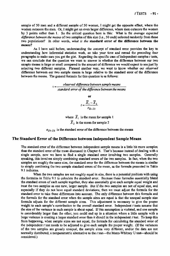
tTESTS -91-
where X1 is the mean for sample 1
X2 is the mean for sample 2
Sx1-x2 is the standard error of the difference between the means
The Standard Error of the Difference between Independent Sample Means
The standard error of the difference between independent sample means is a little bit more complexthan the standard error of the mean discussed in Chapter 6. That's because instead of dealing with asingle sample, now we have to find a single standard error involving two samples. Generallyspeaking, this involves simply combining standard errors of the two samples. In fact, when the twosamples are roughly the same size, the standard error for the difference between the means is similarto simply combining the two sample standard errors of the mean, as the formula presented in Table9.1 indicates.
When the two samples are not roughly equal in size, there is a potential problem with usingthe formulas in Table 9.1 to calculate the standard error. Because these formulas essentially blendthe standard errors of each sample together, they also essentially give each sample equal weight andtreat the two samples as one new, larger sample. But if the two samples are not of equal size, andespecially if they do not have equal standard deviations, then we must adjust the formula for thestandard error to take these differences into account. The only difference between this formula andthe formula for the standard error when the sample sizes are equal is that the unequal sample sizeformula adjusts for the different sample sizes. This adjustment is necessary to give the properweight to each sample's contribution to the overall standard error. Independent t tests assume thatthe size of the variance in each sample is about equal. If this assumption is violated, and one sampleis considerably larger than the other, you could end up in a situation where a little sample with alarge variance is creating a larger standard error than it should in the independent t test. To keep thisfrom happening, when sample sizes are not equal, the formula for calculating the standard error ofthe independent t test needs to be adjusted to give each sample the proper weight. (If the variancesof the two samples are grossly unequal, the sample sizes very different, and/or the data are notnormally distributed, a nonparametric alternative to the t test—the Mann-Whitney U test—should beconsidered.)
sample of 50 men and a different sample of 50 women, I might get the opposite effect, where thewomen outscore the men. Or, I might get an even larger difference, where men outscore the womenby 3 points rather than 1. So the critical question here is this: What is the average expecteddifference between the means of two samples of this size (i.e., 50 each) selected randomly from thesetwo populations? In other words, what is the standard error of the difference between themeans?
As I have said before, understanding the concept of standard error provides the key tounderstanding how inferential statistics work, so take your time and reread the preceding fourparagraphs to make sure you get the gist. Regarding the specific case of independent samples t tests,we can conclude that the question we want to answer is whether the difference between our twosample means is large or small compared to the amount of difference we would expect to see just byselecting two different samples. Phrased another way, we want to know whether our observeddifference between our two sample means is large relative to the standard error of the differencebetween the means. The general formula for this question is as follows:
_ observed difference between sample means
standard error of the difference between the means
or
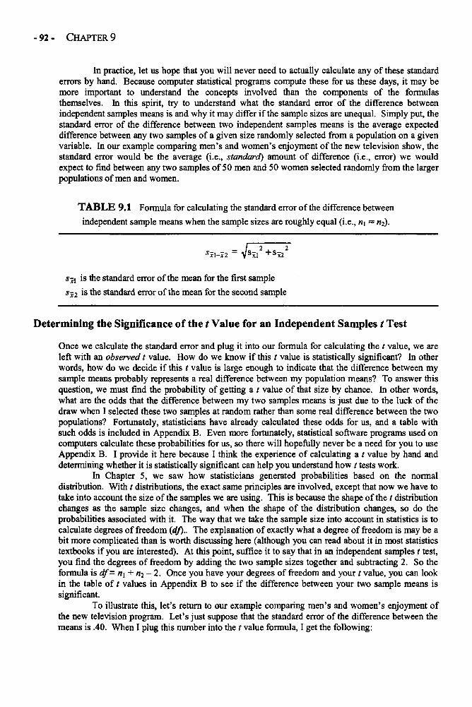
- 92 - CHAPTER 9
In practice, let us hope that you will never need to actually calculate any of these standarderrors by hand. Because computer statistical programs compute these for us these days, it may bemore important to understand the concepts involved than the components of the formulasthemselves. In this spirit, try to understand what the standard error of the difference betweenindependent samples means is and why it may differ if the sample sizes are unequal. Simply put, thestandard error of the difference between two independent samples means is the average expecteddifference between any two samples of a given size randomly selected from a population on a givenvariable. In our example comparing men's and women's enjoyment of the new television show, thestandard error would be the average (i.e., standard) amount of difference (i.e., error) we wouldexpect to find between any two samples of 50 men and 50 women selected randomly from the largerpopulations of men and women.
TABLE 9.1 Formula for calculating the standard error of the difference between
independent sample means when the sample sizes are roughly equal (i.e., n1 ~ n2).
Determining the Significance of the t Value for an Independent Samples t Test
Once we calculate the standard error and plug it into our formula for calculating the t value, we areleft with an observed t value. How do we know if this t value is statistically significant? In otherwords, how do we decide if this t value is large enough to indicate that the difference between mysample means probably represents a real difference between my population means? To answer thisquestion, we must find the probability of getting a t value of that size by chance. In other words,what are the odds that the difference between my two samples means is just due to the luck of thedraw when I selected these two samples at random rather than some real difference between the twopopulations? Fortunately, statisticians have already calculated these odds for us, and a table withsuch odds is included in Appendix B. Even more fortunately, statistical software programs used oncomputers calculate these probabilities for us, so there will hopefully never be a need for you to useAppendix B. I provide it here because I think the experience of calculating a t value by hand anddetermining whether it is statistically significant can help you understand how t tests work.
In Chapter 5, we saw how statisticians generated probabilities based on the normaldistribution. With t distributions, the exact same principles are involved, except that now we have totake into account the size of the samples we are using. This is because the shape of the t distributionchanges as the sample size changes, and when the shape of the distribution changes, so do theprobabilities associated with it. The way that we take the sample size into account in statistics is tocalculate degrees of freedom (df).. The explanation of exactly what a degree of freedom is may be abit more complicated than is worth discussing here (although you can read about it in most statisticstextbooks if you are interested). At this point, suffice it to say that in an independent samples t test,you find the degrees of freedom by adding the two sample sizes together and subtracting 2. So theformula is df- n1 + n2 - 2. Once you have your degrees of freedom and your t value, you can lookin the table of t values in Appendix B to see if the difference between your two sample means issignificant.
To illustrate this, let's return to our example comparing men's and women's enjoyment ofthe new television program. Let's just suppose that the standard error of the difference between themeans is .40. When I plug this number into the t value formula, I get the following:
sx1 is the standard error of the mean for the first sample
sx2 is the standard error of the mean for the second sample
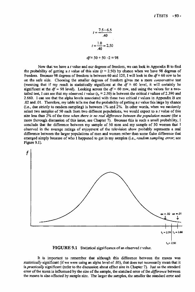
t TESTS -93-
Now that we have a t value and our degrees of freedom, we can look in Appendix B to findthe probability of getting a t value of this size (t = 2.50) by chance when we have 98 degrees offreedom. Because 98 degrees of freedom is between 60 and 120, I will look in the df- 60 row to beon the safe side. Choosing the smaller degrees of freedom gives me a more conservative test(meaning that if my result is statistically significant at the df = 60 level, it will certainly besignificant at the df= 98 level). Looking across the d f = 6 0 row, and using the values for a two-tailed test, I can see that my observed t value (t0 - 2.50) is between the critical t values of 2.390 and2.660. I can see that the alpha levels associated with these two critical t values in Appendix B are.02 and .01. Therefore, my table tells me that the probability of getting a t value this large by chance(i.e., due strictly to random sampling) is between 1% and 2%. In other words, when we randomlyselect two samples of 50 each from two different populations, we would expect to a t value of thissize less than 2% of the time when there is no real difference between the population means (for amore thorough discussion of this issue, see Chapter 7). Because this is such a small probability, Iconclude that the difference between my sample of 50 men and my sample of 50 women that Iobserved in the average ratings of enjoyment of the television show probably represents a realdifference between the larger populations of men and women rather than some fluke difference thatemerged simply because of who I happened to get in my samples (i.e., random sampling error; seeFigure 9.1).
FIGURE 9.1 Statistical significance of an observed t value.
It is important to remember that although this difference between the means wasstatistically significant (if we were using an alpha level of .05), that does not necessarily mean that itis practically significant (refer to the discussion about effect size in Chapter 7). Just as the standarderror of the mean is influenced by the size of the sample, the standard error of the difference betweenthe means is also affected by sample size. The larger the samples, the smaller the standard error and
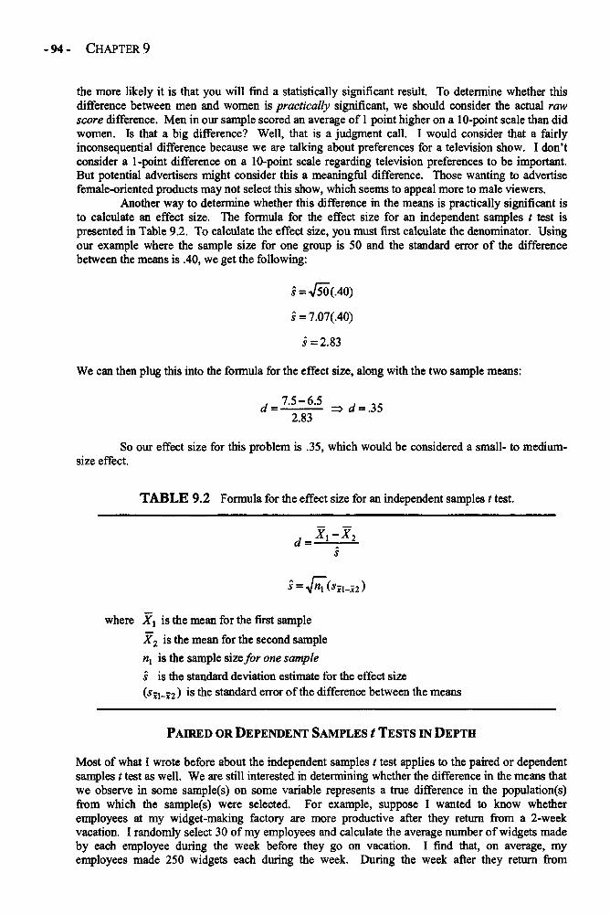
- 94 - CHAPTER 9
the more likely it is that you will find a statistically significant result. To determine whether thisdifference between men and women is practically significant, we should consider the actual rawscore difference. Men in our sample scored an average of 1 point higher on a 10-point scale than didwomen. Is that a big difference? Well, that is a judgment call. I would consider that a fairlyinconsequential difference because we are talking about preferences for a television show. I don'tconsider a 1-point difference on a 10-point scale regarding television preferences to be important.But potential advertisers might consider this a meaningful difference. Those wanting to advertisefemale-oriented products may not select this show, which seems to appeal more to male viewers.
Another way to determine whether this difference in the means is practically significant isto calculate an effect size. The formula for the effect size for an independent samples t test ispresented in Table 9.2. To calculate the effect size, you must first calculate the denominator. Usingour example where the sample size for one group is 50 and the standard error of the differencebetween the means is .40, we get the following:
We can then plug this into the formula for the effect size, along with the two sample means:
So our effect size for this problem is .35, which would be considered a small- to medium-size effect.
TABLE 9.2 Formula for the effect size for an independent samples t test.
where Xl is the mean for the first sample
X2 is the mean for the second sample
n1 is the sample size for one sample
s is the standard deviation estimate for the effect size(sx - x 2) is the standard error of the difference between the means
PAIRED OR DEPENDENT SAMPLES t TESTS IN DEPTH
Most of what I wrote before about the independent samples t test applies to the paired or dependentsamples t test as well. We are still interested in determining whether the difference in the means thatwe observe in some sample(s) on some variable represents a true difference in the population(s)from which the sample(s) were selected. For example, suppose I wanted to know whetheremployees at my widget-making factory are more productive after they return from a 2-weekvacation. I randomly select 30 of my employees and calculate the average number of widgets madeby each employee during the week before they go on vacation. I find that, on average, myemployees made 250 widgets each during the week. During the week after they return from
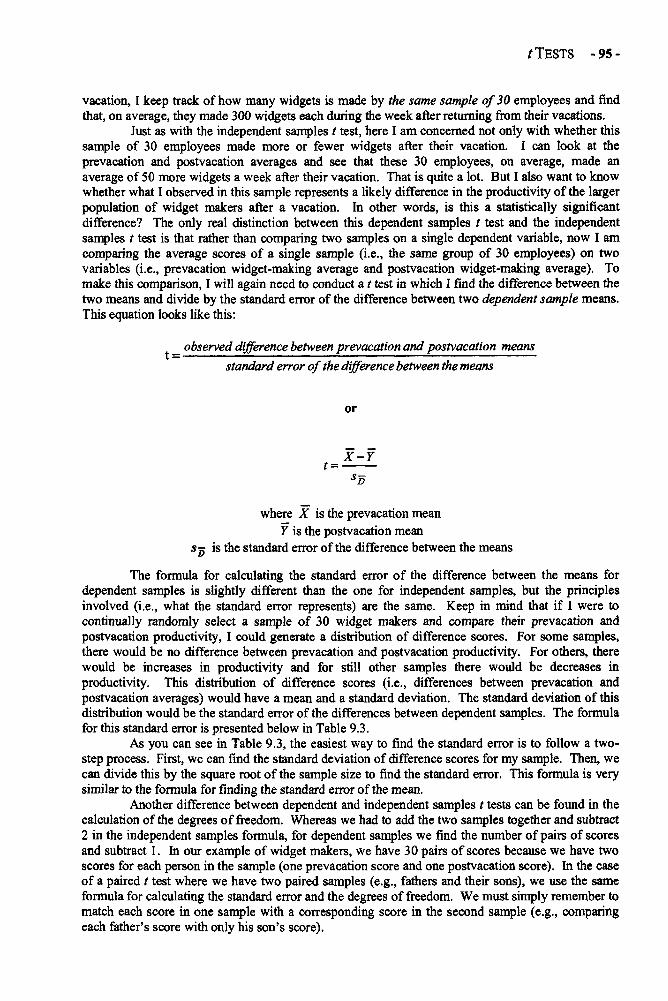
t TESTS -95-
vacation, I keep track of how many widgets is made by the same sample of 30 employees and findthat, on average, they made 300 widgets each during the week after returning from their vacations.
Just as with the independent samples t test, here I am concerned not only with whether thissample of 30 employees made more or fewer widgets after their vacation. I can look at theprevacation and postvacation averages and see that these 30 employees, on average, made anaverage of 50 more widgets a week after their vacation. That is quite a lot. But I also want to knowwhether what I observed in this sample represents a likely difference in the productivity of the largerpopulation of widget makers after a vacation. In other words, is this a statistically significantdifference? The only real distinction between this dependent samples t test and the independentsamples t test is that rather than comparing two samples on a single dependent variable, now I amcomparing the average scores of a single sample (i.e., the same group of 30 employees) on twovariables (i.e., prevacation widget-making average and postvacation widget-making average). Tomake this comparison, I will again need to conduct a t test in which I find the difference between thetwo means and divide by the standard error of the difference between two dependent sample means.This equation looks like this:
_ observed difference between prevacation and postvacation means
standard error of the difference between the means
where X is the prevacation meanY is the postvacation mean
SD is the standard error of the difference between the means
The formula for calculating the standard error of the difference between the means fordependent samples is slightly different than the one for independent samples, but the principlesinvolved (i.e., what the standard error represents) are the same. Keep in mind that if I were tocontinually randomly select a sample of 30 widget makers and compare their prevacation andpostvacation productivity, I could generate a distribution of difference scores. For some samples,there would be no difference between prevacation and postvacation productivity. For others, therewould be increases in productivity and for still other samples there would be decreases inproductivity. This distribution of difference scores (i.e., differences between prevacation andpostvacation averages) would have a mean and a standard deviation. The standard deviation of thisdistribution would be the standard error of the differences between dependent samples. The formulafor this standard error is presented below in Table 9.3.
As you can see in Table 9.3, the easiest way to find the standard error is to follow a two-step process. First, we can find the standard deviation of difference scores for my sample. Then, wecan divide this by the square root of the sample size to find the standard error. This formula is verysimilar to the formula for finding the standard error of the mean.
Another difference between dependent and independent samples t tests can be found in thecalculation of the degrees of freedom. Whereas we had to add the two samples together and subtract2 in the independent samples formula, for dependent samples we find the number of pairs of scoresand subtract 1. In our example of widget makers, we have 30 pairs of scores because we have twoscores for each person in the sample (one prevacation score and one postvacation score). In the caseof a paired t test where we have two paired samples (e.g., fathers and their sons), we use the sameformula for calculating the standard error and the degrees of freedom. We must simply remember tomatch each score in one sample with a corresponding score in the second sample (e.g., comparingeach father's score with only his son's score).
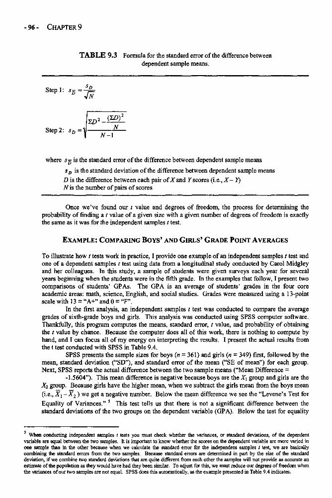
- 96 - CHAPTER 9
TABLE 9.3 Formula for the standard error of the difference betweendependent sample means.
where s-D is the standard error of the difference between dependent sample means
SD is the standard deviation of the difference between dependent sample means
D is the difference between each pair of X and Yscores (i.e., X- Y)N is the number of pairs of scores
Once we've found our t value and degrees of freedom, the process for determining theprobability of finding a t value of a given size with a given number of degrees of freedom is exactlythe same as it was for the independent samples t test.
EXAMPLE: COMPARING BOYS' AND GIRLS' GRADE POINT AVERAGES
To illustrate how t tests work in practice, I provide one example of an independent samples t test andone of a dependent samples t test using data from a longitudinal study conducted by Carol Midgleyand her colleagues. In this study, a sample of students were given surveys each year for severalyears beginning when the students were in the fifth grade. In the examples that follow, I present twocomparisons of students' GPAs. The GPA is an average of students' grades in the four coreacademic areas: math, science, English, and social studies. Grades were measured using a 13-pointscale with 13 = "A+" and 0 = "F".
In the first analysis, an independent samples t test was conducted to compare the averagegrades of sixth-grade boys and girls. This analysis was conducted using SPSS computer software.Thankfully, this program computes the means, standard error, t value, and probability of obtainingthe t value by chance. Because the computer does all of this work, there is nothing to compute byhand, and I can focus all of my energy on interpreting the results. I present the actual results fromthe t test conducted with SPSS in Table 9.4.
SPSS presents the sample sizes for boys (n = 361) and girls (n = 349) first, followed by themean, standard deviation ("SD"), and standard error of the mean ("SE of mean") for each group.Next, SPSS reports the actual difference between the two sample means ("Mean Difference =
-1.5604"). This mean difference is negative because boys are the X\ group and girls are theX2 group. Because girls have the higher mean, when we subtract the girls mean from the boys mean(i.e., X1 -X2) we get a negative number. Below the mean difference we see the "Levene's Test for
Equality of Variances." 5 This test tells us that there is not a significant difference between thestandard deviations of the two groups on the dependent variable (GPA). Below the test for equality
When conducting independent samples t tests you must check whether the variances, or standard deviations, of the dependentvariable are equal between the two samples. It is important to know whether the scores on the dependent variable are more varied inone sample than in the other because when we calculate the standard error for the independent samples t test, we are basicallycombining the standard errors from the two samples. Because standard errors are determined in part by the size of the standarddeviation, if we combine two standard deviations that are quite different from each other the samples will not provide as accurate anestimate of the population as they would have had they been similar. To adjust for this, we must reduce our degrees of freedom whenthe variances of our two samples are not equal. SPSS does this automatically, as the example presented in Table 9.4 indicates.
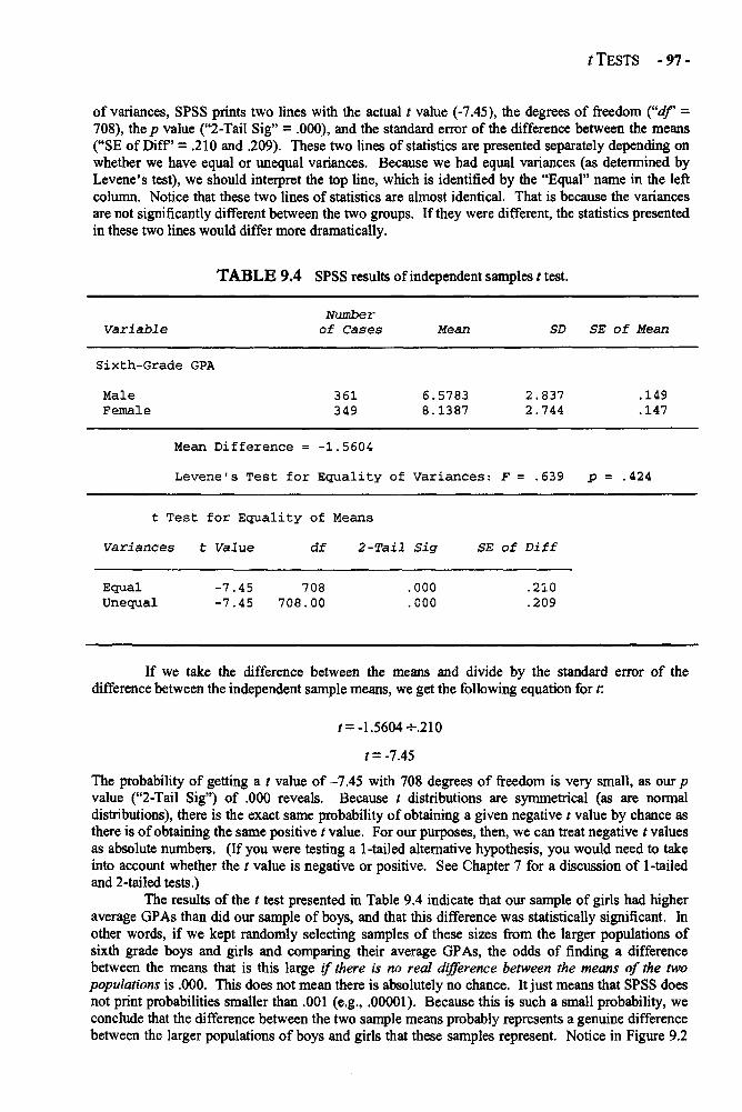
t TESTS -97-
of variances, SPSS prints two lines with the actual t value (-7.45), the degrees of freedom ("df "=708), the p value ("2-Tail Sig" = .000), and the standard error of the difference between the means("SE of Diff" = .210 and .209). These two lines of statistics are presented separately depending onwhether we have equal or unequal variances. Because we had equal variances (as determined byLevene's test), we should interpret the top line, which is identified by the "Equal" name in the leftcolumn. Notice that these two lines of statistics are almost identical. That is because the variancesare not significantly different between the two groups. If they were different, the statistics presentedin these two lines would differ more dramatically.
TABLE 9.4 SPSS results of independent samples t test.
NumberVariable of Cases Mean SD SE of Mean
Sixth-Grade GPA
Male 361 6.5783 2.837 .149Female 349 8.1387 2 .744 .147
Mean Difference = -1.5604
Levene's Test for Equality of Variances: F = .639 p = .424
t Test for Equality of Means
Variances t Value df 2-Tail Sig SE of Diff
Equal -7.45 708 .000 .210Unequal -7.45 708.00 .000 .209
If we take the difference between the means and divide by the standard error of thedifference between the independent sample means, we get the following equation for t:
t = -1.5604 -.210
t = -7.45
The probability of getting a t value of -7.45 with 708 degrees of freedom is very small, as our pvalue ("2-Tail Sig") of .000 reveals. Because t distributions are symmetrical (as are normaldistributions), there is the exact same probability of obtaining a given negative t value by chance asthere is of obtaining the same positive t value. For our purposes, then, we can treat negative t valuesas absolute numbers. (If you were testing a 1-tailed alternative hypothesis, you would need to takeinto account whether the t value is negative or positive. See Chapter 7 for a discussion of 1-tailedand 2-tailed tests.)
The results of the t test presented in Table 9.4 indicate that our sample of girls had higheraverage GPAs than did our sample of boys, and that this difference was statistically significant. Inother words, if we kept randomly selecting samples of these sizes from the larger populations ofsixth grade boys and girls and comparing their average GPAs, the odds of finding a differencebetween the means that is this large if there is no real difference between the means of the twopopulations is .000. This does not mean there is absolutely no chance. It just means that SPSS doesnot print probabilities smaller than .001 (e.g., .00001). Because this is such a small probability, weconclude that the difference between the two sample means probably represents a genuine differencebetween the larger populations of boys and girls that these samples represent. Notice in Figure 9.2
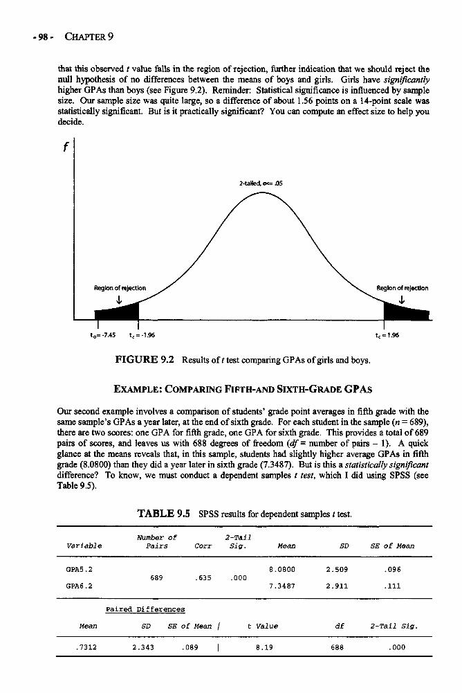
-98- CHAPTER 9
that this observed t value falls in the region of rejection, further indication that we should reject thenull hypothesis of no differences between the means of boys and girls. Girls have significantlyhigher GPAs than boys (see Figure 9.2). Reminder: Statistical significance is influenced by samplesize. Our sample size was quite large, so a difference of about 1.56 points on a 14-point scale wasstatistically significant. But is it practically significant? You can compute an effect size to help youdecide.
FIGURE 9.2 Results of t test comparing GPAs of girls and boys.
EXAMPLE: COMPARING FIFTH-AND SIXTH-GRADE GPAs
Our second example involves a comparison of students' grade point averages in fifth grade with thesame sample's GPAs a year later, at the end of sixth grade. For each student in the sample (n = 689),there are two scores: one GPA for fifth grade, one GPA for sixth grade. This provides a total of 689pairs of scores, and leaves us with 688 degrees of freedom (df- number of pairs - 1). A quickglance at the means reveals that, in this sample, students had slightly higher average GPAs in fifthgrade (8.0800) than they did a year later in sixth grade (7.3487). But is this a statistically significantdifference? To know, we must conduct a dependent samples t test, which I did using SPSS (seeTable 9.5).
TABLE 9.5 SPSS results for dependent samples t test.
Variable
GPA5 . 2
GPA6.2
Number ofPairs
689
2-TailCorr Sig.
.635 .000
Mean
8.0800
7.3487
SD
2.509
2.911
SE of Mean
.096
.111
Paired Differences
Mean SD SE of Mean / t Value df 2-Tail Sig.
.7312 2.343 .089 8.19 688 .000
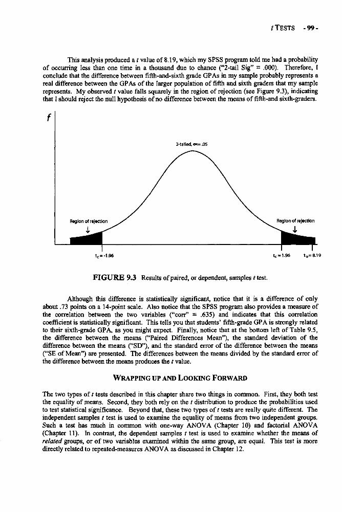
t TESTS -99-
This analysis produced a t value of 8.19, which my SPSS program told me had a probabilityof occurring less than one time in a thousand due to chance ("2-tail Sig" = .000). Therefore, Iconclude that the difference between fifth-and-sixth grade GPAs in my sample probably represents areal difference between the GPAs of the larger population of fifth and sixth graders that my samplerepresents. My observed t value falls squarely in the region of rejection (see Figure 9.3), indicatingthat I should reject the null hypothesis of no difference between the means of fifth-and sixth-graders.
FIGURE 9.3 Results of paired, or dependent, samples t test.
Although this difference is statistically significant, notice that it is a difference of onlyabout .73 points on a 14-point scale. Also notice that the SPSS program also provides a measure ofthe correlation between the two variables ("corr" = .635) and indicates that this correlationcoefficient is statistically significant. This tells you that students' fifth-grade GPA is strongly relatedto their sixth-grade GPA, as you might expect. Finally, notice that at the bottom left of Table 9.5,the difference between the means ("Paired Differences Mean"), the standard deviation of thedifference between the means ("SD"), and the standard error of the difference between the means("SE of Mean") are presented. The differences between the means divided by the standard error ofthe difference between the means produces the t value.
WRAPPING UP AND LOOKING FORWARD
The two types of t tests described in this chapter share two things in common. First, they both testthe equality of means. Second, they both rely on the t distribution to produce the probabilities usedto test statistical significance. Beyond that, these two types of t tests are really quite different. Theindependent samples t test is used to examine the equality of means from two independent groups.Such a test has much in common with one-way ANOVA (Chapter 10) and factorial ANOVA(Chapter 11). In contrast, the dependent samples t test is used to examine whether the means ofrelated groups, or of two variables examined within the same group, are equal. This test is moredirectly related to repeated-measures ANOVA as discussed in Chapter 12.
- 100 - CHAPTER 9
GLOSSARY OF TERMS AND SYMBOLS FOR CHAPTER 9
Categorical, nominal: When variables are measured using categories, or names.Continuous, intervally scaled: When variables are measured using numbers along a continuum
with equal distances, or values, between each number along the continuum.Dependent variable: A variable for which the values may depend on, or differ by, the value of the
independent variable. When the dependent variable is statistically related to theindependent variable, the value of the dependent variable "depends" on, or is predicted by,the value of the independent variable.
Dependent, or paired, samples t test: A test of the statistical similarity between the means of twopaired, or dependent, samles.
Independent samples t test: A test of the statistical similarity between the means of twoindependent samples on a single variable.
Independent variable: A variable that may predict or produce variation in the dependent variable.The independent variable may be nominal or continuous and is sometimes manipulated bythe researcher (e.g., when the researcher assigns participants to an experimental or controlgroup, thereby creating a two-category independent variable).
Matched, paired, dependent samples: When each score of one sample is matched to one scorefrom a second sample. Or, in the case of a single sample measured at two times, when eachscore at Time 1 is matched with the score for the same individual at Time 2.
Matched, paired, dependent samples t test: Test comparing the means of paired, matched, ordependent samples on a single variable.
Significant: Shortened form of the expression "statistically significant."Standard error of the difference between the means: A statistic indicating the standard deviation
of the sampling distribution of the difference between the means.
Sx1-x2 The standard error of difference between two independent sample means.
SD The standard error of the difference between two dependent, or paired sample means.
SD The standard deviation of the difference between two dependent, or paired sample means.
df Degrees of freedom.t The t value.
CHAPTER 10
ONE-WAY ANALYSIS OF VARIANCE
The purpose of a one-way analysis of variance (one-way ANOVA) is to compare the means of twoor more groups (the independent variable) on one dependent variable to see if the group means aresignificantly different from each other. In fact, if you want to compare the means of twoindependent groups on a single variable, you can use either an independent samples t test or a one-way ANOVA. The results will be identical, except instead of producing a t value, the ANOVA willproduce an F ratio, which is simply the t value squared (more about this in the next section of thischapter). Because the t test and the one-way ANOVA produce identical results when there are onlytwo groups being compared, most researchers use the one-way ANOVA only when they arecomparing three or more groups. To conduct a one-way ANOVA, you need to have a categorical (ornominal) variable that has at least two independent groups (e.g., a race variable with the categoriesAfrican-American, Latino, and Euro-American) as the independent variable and a continuousvariable (e.g., achievement test scores) as the dependent variable.
Because the independent t test and the one-way ANOVA are so similar, people oftenwonder, Why don't we just use t tests instead of one-way ANOVAs? Perhaps the best way toanswer this question is by using an example. Suppose that I want to go into the potato chip business.I've got three different recipes, but because I'm new to the business and don't have a lot of money, Ican produce only one flavor. I want to see which flavor people like best and produce that one. Irandomly select 90 adults and randomly divide them into three groups. One group tries my BBQ-flavored chips, the second group tries my ranch-flavored chips, and the third group tastes my cheese-flavored chips. All participants in each group fill out a rating form after tasting the chips to indicatehow much they liked the taste of the chips. The rating scale goes from a score of 1 ("hated it") to 7("loved it"). I then compare the average ratings of the three groups to see which group liked thetaste of their chips the most. In this example, the chip flavor (BBQ, Ranch, Cheese) is mycategorical, independent variable and the rating of the taste of the chips is my continuous, dependentvariable.
To see which flavor received the highest average rating, I could run three separateindependent t tests comparing (a) BBQ with Ranch, (b) BBQ with Cheese, and (c) Ranch withCheese. The problem with running three separate t tests is that each time we run a t test, we mustmake a decision about whether the difference between the two means is meaningful, or statisticallysignificant. This decision is based on probability, and every time we make such a decision, there is aslight chance we might be wrong (see Chapter 7 on statistical significance). The more times wemake decisions about the significance of t tests, the greater the chances are that we will be wrong. Inother words, the more t tests we run, the greater the chances become of deciding that a t test issignificant (i.e., that the means being compared are really different) when it really is not. In stillother words, running multiple t tests increases the likelihood of making a Type I error (i.e., rejectingthe null hypothesis when, in fact, it is true). A one-way ANOVA fixes this problem by adjusting forthe number of groups being compared. To see how it does this, let's take a look at one-wayANOVA in more detail.
ONE-WAY ANOVA IN DEPTH
The purpose of a one-way ANOVA is to divide up the variance in some dependent variable into twocomponents: the variance attributable to between-group differences, and the variance attributable towithin-group differences, also known as error. When we select a sample from a population and
-101-

-102- CHAPTER 10
calculate the mean for that sample on some variable, that sample mean is our best predictor of thepopulation mean. In other words, if we do not know the mean of the population, our best guessabout what the population mean is would have to come from the mean of a sample drawn randomlyfrom that population. Any scores in the sample that differ from the sample mean are believed toinclude what statisticians call error. For example, suppose I have a sample of 20 randomly selectedfifth graders. I give them a test of basic skills in math and find out that, in my sample, the averagenumber of items answered correctly on my test is 12. If I were to select one student in my sampleand find that she had a score of 10 on the test, the difference between her score and the sample meanwould be considered error (see Figure 10.1).
FIGURE 10.1 An example of within-group error.
The variation that we find among the scores in a sample is not just considered error. In fact,it is thought to represent a specific kind of error: random error. When we select a sample atrandom from a population, we expect that the members of that sample will not all have identicalscores on our variable of interest (e.g., test scores). That is, we expect that there will be somevariability in the scores of the members of the sample. That's just what happens when you selectmembers of a sample randomly from a population. Therefore, the variation in scores that we seeamong the members of our sample is just considered random error.
The question that we can address using ANOVA is this: Is the average amount ofdifference, or variation, between the scores of members of different samples large or small comparedto the average amount of variation within each sample, otherwise known as random error (a.k.a.error)? To answer this question, we have to determine three things. First, we have to calculate theaverage amount of variation within each of our samples. This is called the mean square within(MSW) or the mean square error (MSe). Second, we have to find the average amount of variationbetween the groups. This is called the mean square between (MSb). Once we've found these twostatistics, we must find their ratio by dividing the mean square between by the mean square error.This ratio provides our F value, and when we have our F value we can look at our family of Fdistributions to see if the differences between the groups are statistically significant (see Table 10.1).
Note that, although it may sound like analysis of variance is a whole new concept, in fact itis virtually identical to the independent t test discussed in Chapter 9. Recall that the formula forcalculating an independent t test also involves finding a ratio. The top portion of the fraction is the
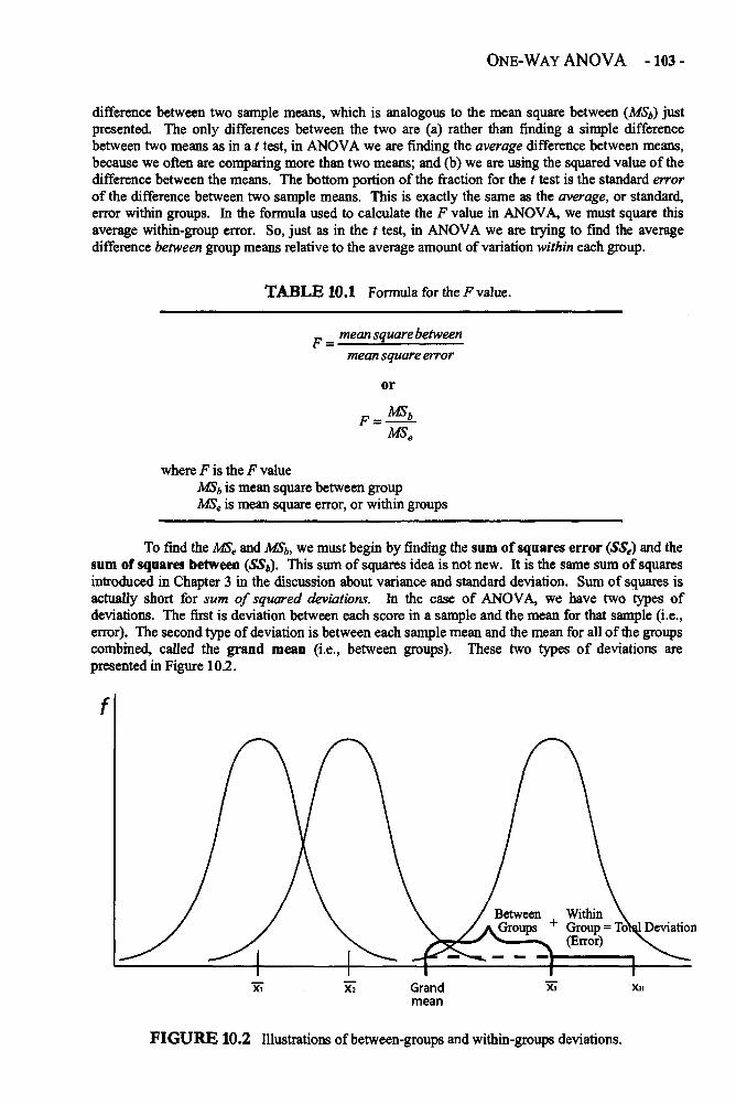
ONE-WAY ANOVA -103 -
difference between two sample means, which is analogous to the mean square between (MSb) justpresented. The only differences between the two are (a) rather than finding a simple differencebetween two means as in a t test, in ANOVA we are finding the average difference between means,because we often are comparing more than two means; and (b) we are using the squared value of thedifference between the means. The bottom portion of the fraction for the t test is the standard errorof the difference between two sample means. This is exactly the same as the average, or standard,error within groups. In the formula used to calculate the F value in ANOVA, we must square thisaverage within-group error. So, just as in the t test, in ANOVA we are trying to find the averagedifference between group means relative to the average amount of variation within each group.
TABLE 10.1 Formula for the F value.
where F is the F valueMSb is mean square between groupMSe is mean square error, or within groups
To find the MSe and MSb we must begin by finding the sum of squares error (SSe) and thesum of squares between (SSb). This sum of squares idea is not new. It is the same sum of squaresintroduced in Chapter 3 in the discussion about variance and standard deviation. Sum of squares isactually short for sum of squared deviations. In the case of ANOVA, we have two types ofdeviations. The first is deviation between each score in a sample and the mean for that sample (i.e.,error). The second type of deviation is between each sample mean and the mean for all of the groupscombined, called the grand mean (i.e., between groups). These two types of deviations arepresented in Figure 10.2.
FIGURE 10.2 Illustrations of between-groups and within-groups deviations.
mean square betweenF =mean square error
or
-104- CHAPTER 10
To find the sum of squares error (SSe):
1. Subtract the group mean from each individual score in each group: (X- X ).
2. Square each of these deviation scores: (X-X)2.
3. Add them all up for each group: E(X-X)2 .
4. Then add up all of the sums of squares for all of the groups:E ( X l - X l ) 2 + E ( X 2 - X 2 ) + . . . + E ( X k - X k ) 2
Note: The subscripts indicate the individual groups, through the last group,which is indicated with the subscript k.
The method used to calculate the sum of squares between groups (SSb) is just slightly morecomplicated than the SSe formula. To find the SSb we
1. Subtract the grand mean from the group mean: ( X - XT ); T indicates total, or the mean
for the total group.
2. Square each of these deviation scores: (X - XT )2.
3. Multiply each squared deviation by the number of cases in the group: [n( X-XT )2].
4. Add these squared deviations from each group together: E[n( X-XT )2].
The only real differences between the formula for calculating the SSe and the SSb are
1. In the SSe we subtract the group mean from the individual scores in each group,whereas in the SSb we subtract the grand mean from each group mean.
2. In the SSb we multiply each squared deviation by the number of cases in eachgroup. We must do this to get an approximate deviation between the group meanand the grand mean for each case in every group.
If we were to add the SSe to the SSb, the resulting sum would be called the sum of squarestotal (SST). A brief word about the SST is in order. Suppose that we have three randomly selectedsamples of children. One is a sample of 5th graders, another is a sample of 8th graders, and the thirdis a sample of 11th graders. If we were to give each student in each sample a spelling test, we couldadd up the scores for all of the children in the three samples combined and divide by the totalnumber of scores to produce one average score. Because we have combined the scores from allthree samples, this overall average score would be called the grand mean, or total mean, whichwould have the symbol XT . Using this grand mean, we could calculate a squared deviation score
for each child in all three of our samples combined using the familiar formula (X - XT )2. The
interesting thing about these squared deviations is that, for each child, the difference between eachchild's score and the grand mean is the sum of that child's deviation from the mean of his or her owngroup plus the deviation of that group mean from the grand mean. So, suppose Jimmy is in the fifth-grade sample. Jimmy gets a score of 25 on the spelling test. The average score for the fifth-gradesample is 30, and the average score for all of the samples combined (i.e., the grand mean) is 35. Thedifference between Jimmy's score (25) and the grand mean (35) is just the difference betweenJimmy's score and the mean for his group (25 - 30 = -5) plus the difference between his group's
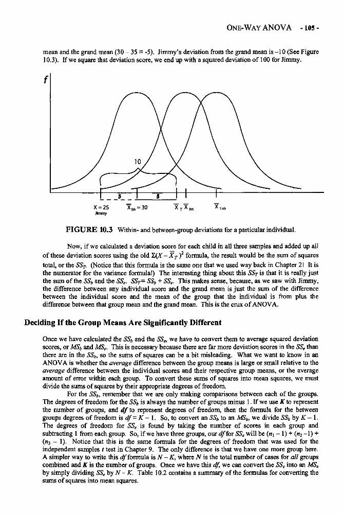
ONE-WAY ANOVA -105 -
mean and the grand mean (30 - 35 = -5). Jimmy's deviation from the grand mean is -10 (See Figure10.3). If we square that deviation score, we end up with a squared deviation of 100 for Jimmy.
FIGURE 10.3 Within- and between-group deviations for a particular individual.
Now, if we calculated a deviation score for each child in all three samples and added up allof these deviation scores using the old E ( X - X T ) 2 formula, the result would be the sum of squares
total, or the SST. (Notice that this formula is the same one that we used way back in Chapter 2! It isthe numerator for the variance formula!) The interesting thing about this SST is that it is really justthe sum of the SSb, and the SSe. SST= SSb + SSe. This makes sense, because, as we saw with Jimmy,the difference between any individual score and the grand mean is just the sum of the differencebetween the individual score and the mean of the group that the individual is from plus thedifference between that group mean and the grand mean. This is the crux of ANOVA.
Deciding If the Group Means Are Significantly Different
Once we have calculated the SSb and the SSe, we have to convert them to average squared deviationscores, or MSb and MSe. This is necessary because there are far more deviation scores in the SSe thanthere are in the SSb, so the sums of squares can be a bit misleading. What we want to know in anANOVA is whether the average difference between the group means is large or small relative to theaverage difference between the individual scores and their respective group means, or the averageamount of error within each group. To convert these sums of squares into mean squares, we mustdivide the sums of squares by their appropriate degrees of freedom.
For the SSb, remember that we are only making comparisons between each of the groups.The degrees of freedom for the SSb is always the number of groups minus 1. If we use K to representthe number of groups, and df to represent degrees of freedom, then the formula for the betweengroups degrees of freedom is df = K- 1. So, to convert an SSb to an MSb, we divide SSb by K - 1.The degrees of freedom for SSe is found by taking the number of scores in each group andsubtracting 1 from each group. So, if we have three groups, our df for SSe will be (n1 - 1) + (n2 -1) +(773 - 1). Notice that this is the same formula for the degrees of freedom that was used for theindependent samples t test in Chapter 9. The only difference is that we have one more group here.A simpler way to write thisdf formula is N - K, where N is the total number of cases for all groupscombined and K is the number of groups. Once we have this df, we can convert the SSe into an MSe
by simply dividing SSe by N - K. Table 10.2 contains a summary of the formulas for converting thesums of squares into mean squares.
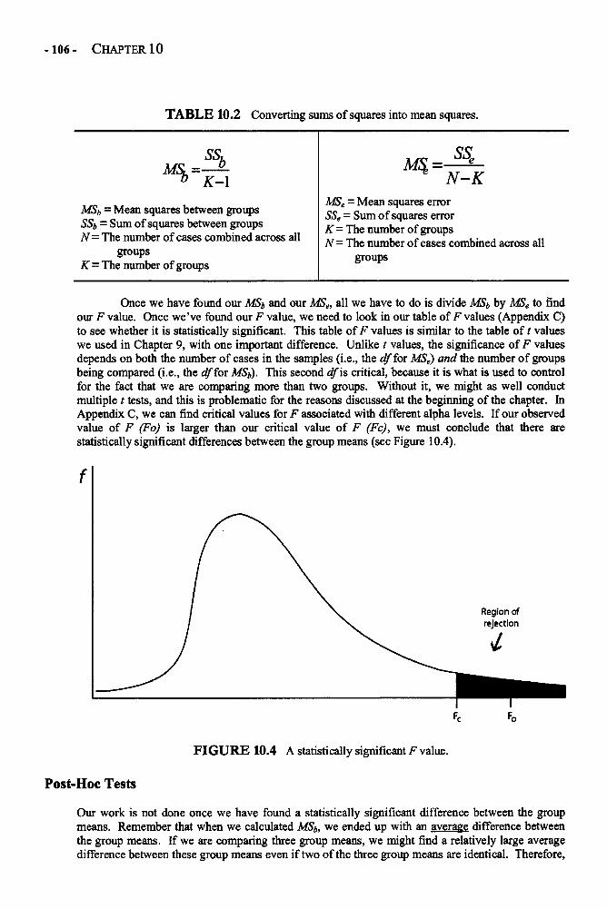
-106- CHAPTER 10
TABLE 10.2 Converting sums of squares into mean squares.
MSb = Mean squares between groupsSSb - Sum of squares between groupsN = The number of cases combined across all
groupsK = The number of groups
MSe = Mean squares errorSSe = Sum of squares errorK = The number of groupsN = The number of cases combined across all
groups
Once we have found our MSb and our MSe, all we have to do is divide MSb by MSe to findour F value. Once we've found our F value, we need to look in our table of F values (Appendix C)to see whether it is statistically significant. This table of F values is similar to the table of t valueswe used in Chapter 9, with one important difference. Unlike t values, the significance of F valuesdepends on both the number of cases in the samples (i.e., the df for MSe) and the number of groupsbeing compared (i.e., the df for MSb). This second df is critical, because it is what is used to controlfor the fact that we are comparing more than two groups. Without it, we might as well conductmultiple t tests, and this is problematic for the reasons discussed at the beginning of the chapter. InAppendix C, we can find critical values for F associated with different alpha levels. If our observedvalue of F (Fo) is larger than our critical value of F (Fc), we must conclude that there arestatistically significant differences between the group means (see Figure 10.4).
FIGURE 10.4 A statistically significant F value.
Post-Hoc Tests
Our work is not done once we have found a statistically significant difference between the groupmeans. Remember that when we calculated MSb, we ended up with an average difference betweenthe group means. If we are comparing three group means, we might find a relatively large averagedifference between these group means even if two of the three group means are identical. Therefore,
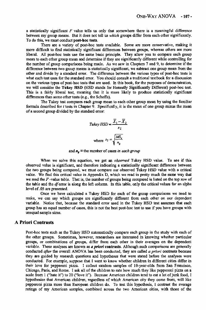
ONE-WAY ANOVA -107 -
a statistically significant F value tells us only that somewhere there is a meaningful differencebetween my group means. But it does not tell us which groups differ from each other significantly.To do this, we must conduct post-hoc tests.
There are a variety of post-hoc tests available. Some are more conservative, making itmore difficult to find statistically significant differences between groups, whereas others are moreliberal. All post-hoc tests use the same basic principle. They allow you to compare each groupmean to each other group mean and determine if they are significantly different while controlling forthe number of group comparisons being made. As we saw in Chapters 7 and 9, to determine if thedifference between two group means is statistically significant, we subtract one group mean from theother and divide by a standard error. The difference between the various types of post-hoc tests iswhat each test uses for the standard error. You should consult a traditional textbook for a discussionon the various types of post-hoc tests that are used. In this book, for the purposes of demonstration,we will consider the Tukey HSD (HSD stands for Honestly Significantly Different) post-hoc test.This is a fairly liberal test, meaning that it is more likely to produce statistically significantdifferences than some other tests (e.g., the Scheffe).
The Tukey test compares each group mean to each other group mean by using the familiarformula described for t tests in Chapter 9. Specifically, it is the mean of one group minus the meanof a second group divided by the standard error:
and ng = the number of cases in each group
When we solve this equation, we get an observed Tukey HSD value. To see if thisobserved value is significant, and therefore indicating a statistically significant difference betweenthe two groups being compared, we must compare our observed Tukey HSD value with a criticalvalue. We find this critical value in Appendix D, which we read in pretty much the same way thatwe read the F -value table. That is, the number of groups being compared is listed on the top row ofthe table and thedf error is along the left column. In this table, only the critical values for an alphalevel of .05 are presented.
Once we have calculated a Tukey HSD for each of the group comparisons we need tomake, we can say which groups are significantly different from each other on our dependentvariable. Notice that, because the standard error used in the Tukey HSD test assumes that eachgroup has an equal number of cases, this is not the best post-hoc test to use if you have groups withunequal sample sizes.
A Priori Contrasts
Post-hoc tests such as the Tukey HSD automatically compare each group in the study with each ofthe other groups. Sometimes, however, researchers are interested in knowing whether particulargroups, or combinations of groups, differ from each other in their averages on the dependentvariable. These analyses are known as a priori contrasts. Although such comparisons are generallyconducted after the overall ANOVA has been conducted, they are called a priori contrasts becausethey are guided by research questions and hypotheses that were stated before the analyses wereconducted. For example, suppose that I want to know whether children in different cities differ intheir love for pepperoni pizza. I collect random samples of 10-year-olds from San Francisco,Chicago, Paris, and Rome. I ask all of the children to rate how much they like pepperoni pizza on ascale from 1 ("hate it") to 20 ("love it"). Because American children tend to eat a lot of junk food, Ihypothesize that American children, regardless of which American city they come from, will likepepperoni pizza more than European children do. To test this hypothesis, I contrast the averageratings of my American samples, combined across the two American cities, with those of the
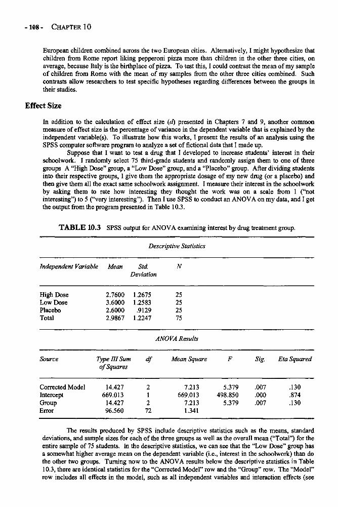
-108- CHAPTER 10
European children combined across the two European cities. Alternatively, I might hypothesize thatchildren from Rome report liking pepperoni pizza more than children in the other three cities, onaverage, because Italy is the birthplace of pizza. To test this, I could contrast the mean of my sampleof children from Rome with the mean of my samples from the other three cities combined. Suchcontrasts allow researchers to test specific hypotheses regarding differences between the groups intheir studies.
Effect Size
In addition to the calculation of effect size (d) presented in Chapters 7 and 9, another commonmeasure of effect size is the percentage of variance in the dependent variable that is explained by theindependent variable(s). To illustrate how this works, I present the results of an analysis using theSPSS computer software program to analyze a set of fictional data that I made up.
Suppose that I want to test a drug that I developed to increase students' interest in theirschoolwork. I randomly select 75 third-grade students and randomly assign them to one of threegroups A "High Dose" group, a "Low Dose" group, and a "Placebo" group. After dividing studentsinto their respective groups, I give them the appropriate dosage of my new drug (or a placebo) andthen give them all the exact same schoolwork assignment. I measure their interest in the schoolworkby asking them to rate how interesting they thought the work was on a scale from 1 ("notinteresting") to 5 ("very interesting"). Then I use SPSS to conduct an ANOVA on my data, and I getthe output from the program presented in Table 10.3.
TABLE 10.3 SPSS output for ANOVA examining interest by drug treatment group.
Descriptive Statistics
High DoseLow DosePlaceboTotal
2.76003.60002.60002.9867
1.26751.2583.9129
1.2247
25252575
ANOVA Results
Source
Corrected ModelInterceptGroupError
Type El Sumof Squares
14.427669.013
14.42796.560
df
212
72
Mean Square
7.213669.013
7.2131.341
F
5.379498.850
5.379
Sig.
.007
.000
.007
Eta Squared
.130
.874
.130
The results produced by SPSS include descriptive statistics such as the means, standarddeviations, and sample sizes for each of the three groups as well as the overall mean ("Total") for theentire sample of 75 students. In the descriptive statistics, we can see that the "Low Dose" group hasa somewhat higher average mean on the dependent variable (i.e., interest in the schoolwork) than dothe other two groups. Turning now to the ANOVA results below the descriptive statistics in Table10.3, there are identical statistics for the "Corrected Model" row and the "Group" row. The "Model"row includes all effects in the model, such as all independent variables and interaction effects (see
Independent Variable Mean Std. NDeviation

ONE-WAYANOVA -109-
Chapter 11 for a discussion of these multiple effects). In the present example, there is only oneindependent variable, so the "Model" statistics are the same as the "Group" statistics.
Let's focus on the "Group" row. This row includes all of the between-group information,because "Group" is our independent group variable. Here we see the Sum of Squares between(SSb),
6 which is 14.427. The degrees of freedom ("df") here is 2, because with three groups, K - 1 =2. The sum of squares divided by degrees of freedom produces the mean square (MSb), which is7.213. The statistics for the sum of squares error (SSe), degrees of freedom for the error component,and mean square error (MSe) are all in the row below the "Group" row. The F value ("F") for thisANOVA is 5.379, which was produced by dividing the mean square from the "Group" row by themean square from the error row. This F value is statistically significant ("Sig." = .007). The "Sig"is the same thing as the p value (described in Chapter 7). Finally, in the "Eta Squared" column, wecan see that we have a value of .130 in the "Group" row. Eta squared is a measure of the associationbetween the independent variable ("Group") and the dependent variable ("Interest"). It indicates that13% of the variance in the scores on the interest variable can be explained by the Group variable. Inother words, I can account for 13% of the variance in the interest scores simply by knowing whetherstudents were in the "High Dose," "Low Dose," or "Placebo" group. Eta squared is essentially thesame as the coefficient of determination (r2) discussed in Chapter 8 and again in Chapter 13.
TABLE 10.4 SPSS results of Tukey HSD post-hoc tests.
(I) Treatment 1, Treatment2, Control
High Dose
Low Dose
Placebo
(J) Treatment 1,Treatment 2, Control
Low Dose
Placebo
High Dose
Placebo
High Dose
Low Dose
Mean Difference(I-J)
-.8400
.1600
.8400
1.0000
-.1600
-1.0000
Std. Error
.328
.328
.328
.328
.328
.328
Sig.
.033
.877
.033
.009
.877
.009
Now that we know mat there is a statistically significant difference between the threegroups in their level of interest, and that group membership accounts for 13% of the variance ininterest scores, it is time to look at our Tukey post-hoc analysis to determine which groupssignificantly differ from each other. The SPSS results of this analysis are presented in Table 10.4.The far left column of this table contains the reference group (I), and the column to the right of thisshows the comparison groups (J). So in the first comparison, the mean for the "High Dose" group iscompared to the mean for the "Low Dose" group. We can see that the "Mean Difference" betweenthese two groups is -.8400, indicating that the "High Dose" group had a mean that was .84 pointslower than the mean of the "Low Dose" group on the interest variable. In the last column, we cansee that this difference is statistically significant ("Sig." = .033). So we can conclude that students inthe "Low Dose" group, on average, were more interested in their work than were students in the"High Dose" group. In the next comparison between "High Dose" and "Placebo" we find a meandifference of .16, which was not significant ("Sig." = .877). Looking at the next set of comparisons,we see that the "Low Dose" group is significantly different from both the "High Dose" group (wealready knew this) and the "Placebo" group. At this point, all of our comparisons have been made
SPSS generally reports this as the Type III sum of squares. This sum of squares is known as the "residual" sum of squares because itis calculated after taking the effects of other independent variables, covariates, and interaction effects into account.
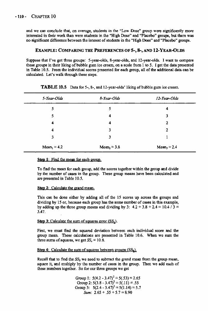
-110- CHAPTER 10
and we can conclude that, on average, students in the "Low Dose" group were significantly moreinterested in their work than were students in the "High Dose" and "Placebo" groups, but there wasno significant difference between the interest of students in the "High Dose" and "Placebo" groups.
EXAMPLE: COMPARING THE PREFERENCES OF 5-, 8-, AND 12-YEAR-OLDS
Suppose that I've got three groups: 5-year-olds, 8-year-olds, and 12-year-olds. I want to comparethese groups in their liking of bubble gum ice cream, on a scale from 1 to 5. I get the data presentedin Table 10.5. From the individual scores presented for each group, all of the additional data can becalculated. Let's walk through these steps.
TABLE 10.5 Data for 5-, 8-, and 12-year-olds' liking of bubble gum ice cream.
5-Year-Olds
5
5
4
4
3
Mean1 = 4.2
8-Year-Olds
5
4
4
3
3
Mean2 = 3.8
12-Year-Olds
4
3
2
2
1
Mean3 = 2 .4
Step 1: Find the mean for each group.
To find the mean for each group, add the scores together within the group and divideby the number of cases in the group. These group means have been calculated andare presented in Table 10.5.
Step 2: Calculate the grand mean.
This can be done either by adding all of the 15 scores up across the groups anddividing by 15 or, because each group has the same number of cases in this example,by adding up the three group means and dividing by 3: 4.2 + 3.8 + 2.4 = 10.4 / 3 =3.47.
Step 3: Calculate the sum of squares error (SSe).
First, we must find the squared deviation between each individual score and thegroup mean. These calculations are presented in Table 10.6. When we sum thethree sums of squares, we get SSe - 10.8.
Step 4: Calculate the sum of squares between groups (SSb).
Recall that to find the SSb we need to subtract the grand mean from the group mean,square it, and multiply by the number of cases in the group. Then we add each ofthese numbers together. So for our three groups we get
Group 1: 5(4.2 - 3.47)2 = 5(.53) = 2.65Group 2: 5(3.8 - 3.47)2 = 5(.l 1) = .55
Group 3: 5(2.4 - 3.47)2 = 5(1.14) = 5.7Sum: 2.65+ .55+5.7 = 8.90
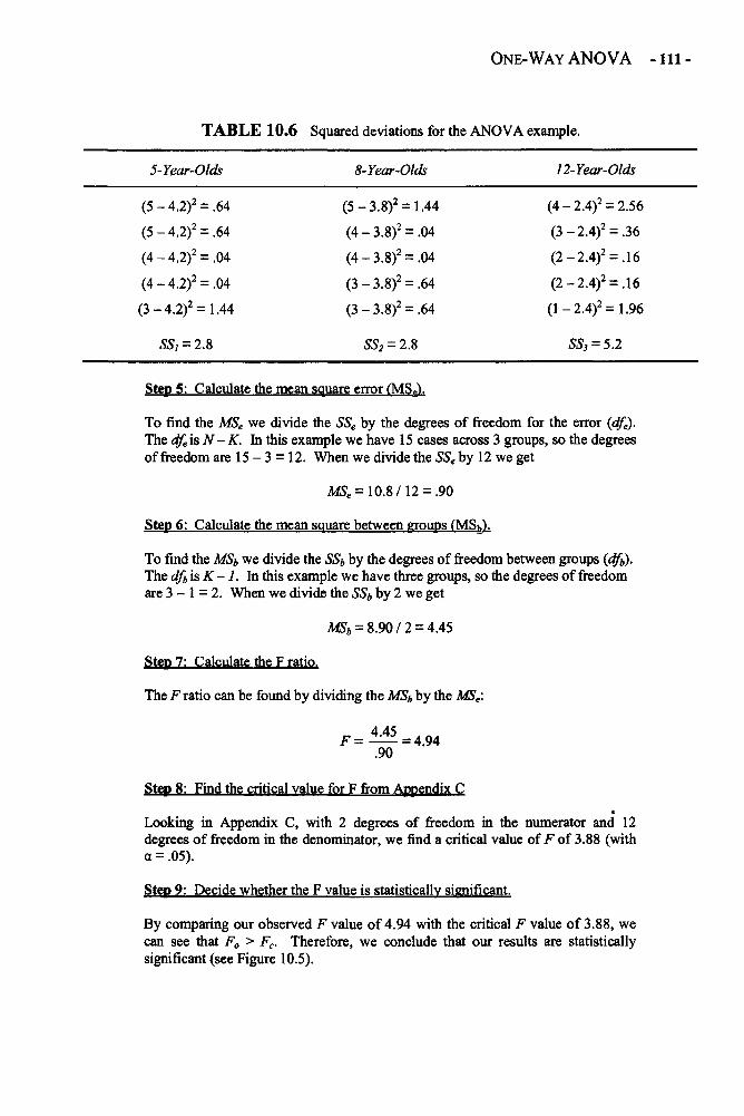
ONE-WAY ANOVA -111-
TABLE 10.6 Squared deviations for the ANOVA example.
5-Year-Olds
(5
(5
-4
-4
•2)2 =
•2)2 =
(4-4.2)2 =
(4
(3
-4
-4.
.2)2 =
2)2 =
.64
.64
.04
.04
1.44
8-Year-Olds
(5.
(4
(4
(3
(3
SSI = 2.8
- 3.8)2 = 1
-3.
-3._ 3
-3.
SS2
8)2 =
8)2 =
8)2 =
8)2 =
= 2.8
.44
.04
.04
.64
.64
12-Year-Olds
(4
(3
(2
(2
(1
_ 2
-2
-2
-2
-2.
4)2 = 2.56
•4)2 = .
.4)2 = .
•4)2 = .
4)2 = 1
36
16
16
.96
SS3 = 5.2
Step 5: Calculate the mean square error (MSe).
To find the MSe we divide the SSe by the degrees of freedom for the error (dfe).The dfe is N - K. In this example we have 15 cases across 3 groups, so the degreesof freedom are 15 - 3 = 12. When we divide the SSe by 12 we get
MSe = 10.8 / 12 = .90
Step 6: Calculate the mean square between groups (MSb).
To find the MSb we divide the SSb by the degrees of freedom between groups (dfb).The dfb is K -1. In this example we have three groups, so the degrees of freedomare 3 - 1 = 2. When we divide the SSb by 2 we get
MSb = 8.90 / 2 = 4.45
Step 7: Calculate the F ratio.
The F ratio can be found by dividing the MSb by the MSE:
Step 8: Find the critical value for F from Appendix C<
Looking in Appendix C, with 2 degrees of freedom in the numerator and 12degrees of freedom in the denominator, we find a critical value of F of 3.88 (witha = .05).
Step 9: Decide whether the F value is statistically significant.
By comparing our observed F value of 4.94 with the critical F value of 3.88, wecan see that Fo > Fc. Therefore, we conclude that our results are statisticallysignificant (see Figure 10.5).
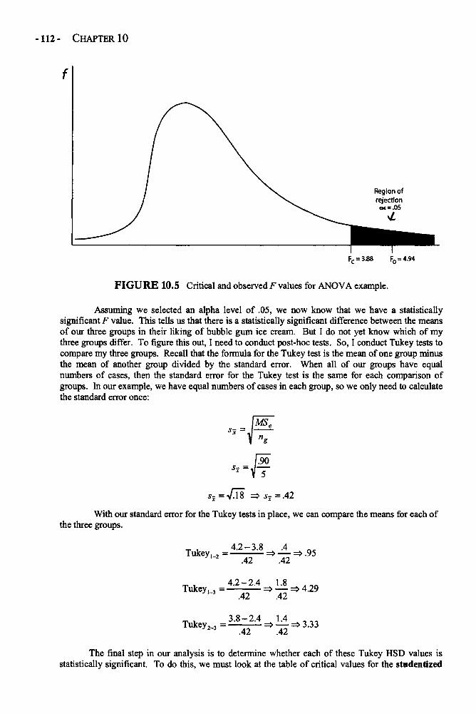
-112- CHAPTER 10
FIGURE 10.5 Critical and observed F values for ANOVA example.
Assuming we selected an alpha level of .05, we now know that we have a statisticallysignificant F value. This tells us that there is a statistically significant difference between the meansof our three groups in their liking of bubble gum ice cream. But I do not yet know which of mythree groups differ. To figure this out, I need to conduct post-hoc tests. So, I conduct Tukey tests tocompare my three groups. Recall that the formula for the Tukey test is the mean of one group minusthe mean of another group divided by the standard error. When all of our groups have equalnumbers of cases, then the standard error for the Tukey test is the same for each comparison ofgroups. In our example, we have equal numbers of cases in each group, so we only need to calculatethe standard error once:
With our standard error for the Tukey tests in place, we can compare the means for each ofthe three groups.
The final step in our analysis is to determine whether each of these Tukey HSD values isstatistically significant. To do this, we must look at the table of critical values for the studentized
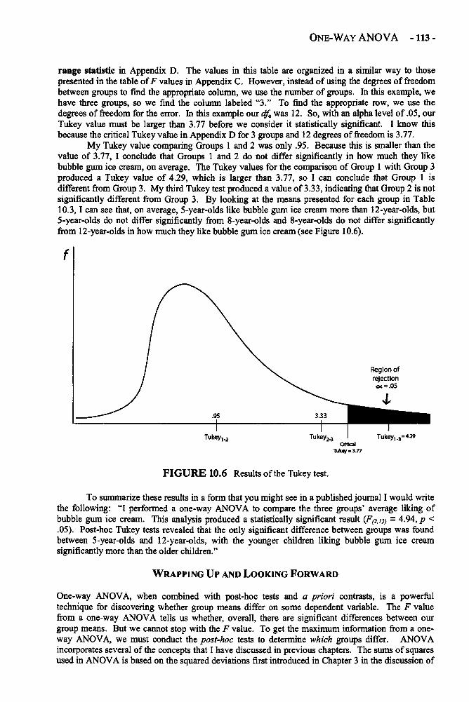
ONE-WAY ANOVA -113-
range statistic in Appendix D. The values in this table are organized in a similar way to thosepresented in the table of F values in Appendix C. However, instead of using the degrees of freedombetween groups to find the appropriate column, we use the number of groups. In this example, wehave three groups, so we find the column labeled "3." To find the appropriate row, we use thedegrees of freedom for the error. In this example our dfe was 12. So, with an alpha level of .05, ourTukey value must be larger than 3.77 before we consider it statistically significant. I know thisbecause the critical Tukey value in Appendix D for 3 groups and 12 degrees of freedom is 3.77.
My Tukey value comparing Groups 1 and 2 was only .95. Because this is smaller than thevalue of 3.77, I conclude that Groups 1 and 2 do not differ significantly in how much they likebubble gum ice cream, on average. The Tukey values for the comparison of Group 1 with Group 3produced a Tukey value of 4.29, which is larger than 3.77, so I can conclude that Group 1 isdifferent from Group 3. My third Tukey test produced a value of 3.33, indicating that Group 2 is notsignificantly different from Group 3. By looking at the means presented for each group in Table10.3, I can see that, on average, 5-year-olds like bubble gum ice cream more than 12-year-olds, but5-year-olds do not differ significantly from 8-year-olds and 8-year-olds do not differ significantlyfrom 12-year-olds in how much they like bubble gum ice cream (see Figure 10.6).
FIGURE 10.6 Results of the Tukey test.
To summarize these results in a form that you might see in a published journal I would writethe following: "I performed a one-way ANOVA to compare the three groups' average liking ofbubble gum ice cream. This analysis produced a statistically significant result (F(2,12) - 4.94, p <.05). Post-hoc Tukey tests revealed that the only significant difference between groups was foundbetween 5-year-olds and 12-year-olds, with the younger children liking bubble gum ice creamsignificantly more than the older children."
WRAPPING UP AND LOOKING FORWARD
One-way ANOVA, when combined with post-hoc tests and a priori contrasts, is a powerfultechnique for discovering whether group means differ on some dependent variable. The F valuefrom a one-way ANOVA tells us whether, overall, there are significant differences between ourgroup means. But we cannot stop with the F value. To get the maximum information from a one-way ANOVA, we must conduct the post-hoc tests to determine which groups differ. ANOVAincorporates several of the concepts that I have discussed in previous chapters. The sums of squaresused in ANOVA is based on the squared deviations first introduced in Chapter 3 in the discussion of
-114- CHAPTER 10
variance. The comparisons of group means is similar to the information about independent samples ttests presented in Chapter 9. And the eta-squared statistic, which is a measure of associationbetween the independent and dependent variables, is related to the concepts of shared variance andvariance explained discussed in Chapter 8 as well as the notion of effect size discussed in Chapter 7.
In this chapter, a brief introduction to the most basic ANOVA model and post-hoc tests wasprovided. It is important to remember that many models are not this simple. In the real world ofsocial science research, it is often difficult to find groups with equal numbers of cases. When groupshave different numbers of cases, the ANOVA model becomes a bit more complicated. I encourageyou to read more about one-way ANOVA models, and I offer some references to help you learnmore. In the next two chapters, I examine two more advanced types of ANOVA techniques:factorial ANOVA and repeated-measures ANOVA.
In this chapter and those that preceded it, I examined several of the most basic, and mostcommonly used, statistics in the social sciences. These statistics form the building blocks for mostof the more advanced techniques used by researchers. For example, t tests and one-way ANOVArepresent the basic techniques for examining the relations between nominal or categoricalindependent variables and continuous dependent variables. More advanced methods of examiningsuch relations, such as factorial ANOVA and repeated-measures ANOVA are merely elaborations ofthe more basic methods I have already discussed. Similarly, techniques for examining the relationsamong two or more continuous variables are all based on the statistical technique already discussedin Chapter 8, correlations. More advanced techniques, such as factor analysis and regression, arebased on correlations.
In the remaining chapters of this book, three of more advanced statistical techniques aredescribed. Because the purpose of this book is to provide a short, nontechnical description of anumber of statistical methods commonly used by social scientists, there is not adequate space toprovide detailed descriptions of these more advanced techniques. Specifically, the technicaldescriptions of the formulas used to generate these statistics is beyond the scope and purpose of thisbook. Therefore, in the chapters that follow, general descriptions of each technique are provided,including what the technique does, when to use it, and an example of results generated from astatistical analysis using the technique. Suggestions for further reading on each technique are alsoprovided.
GLOSSARY OF TERMS AND SYMBOLS FOR CHAPTER 10
a priori contrasts: Comparisons of means that are planned before the ANOVA is conducted. Caninclude comparing the mean of one group to two or more other groups combined.
Between group: Refers to effects (e.g., variance, differences) that occur between the members ofdifferent groups in an ANOVA.
F value: The statistic used to indicate the average amount of difference between group meansrelative to the average amount of variance within each group.
Grand mean: The statistical average for all of the cases in all of the groups on the dependentvariable.
Mean square between: The average squared deviation between the group means and the grandmean.
Mean square error: The average squared deviation between each individual and their respectivegroup means.
Mean square within: The average squared deviation between each group mean and the individualscores within each group.
One-way ANOVA: Analysis of variance conducted to test whether two or more group means differsignificantly on a single dependent variable.
Post-hoc tests: Statistical tests conducted after obtaining the overall F value from the ANOVA toexamine whether each group mean differs significantly from each other group mean.
Random error: Refers to differences between individual scores and sample means that arepresumed to occur simply because of the random effects inherent in selecting cases for the
ONE-WAY ANOVA -115-
sample. (Note that random error, more broadly, refers to differences between sample dataor statistics and population data or parameters caused by random selection procedures.)
Studentized range statistic: Distributions used to determine the statistical significance of post-hoctests.
Sum of squares between: Sum of the squared deviations between the group means and the grandmean.
Sum of squares error: Sum of the squared deviations between individual scores and group meanson the dependent variable.
Sum of squares total: Sum of the squared deviations between individual scores and the grand meanon the dependent variable. This is also the sum of the SSb and the SSe.
Within-group: Refers to effects (e.g., variance, differences) that occur between the members of thesame groups in an ANOVA.
Tukey HSD: Name of a common post-hoc test.
MSW Mean square within groups.MSe Mean square error (which is the same as the mean square within groups).MSb Mean square between groups.SSe Sum of squares error (or within groups).SSb Sum of squares between groups.SST Sum of squares total.XT The grand mean.
F The F value.df Degrees of freedom.K The number of groups.N The number of cases in all of the groups combined.n The number of cases in a given group (for calculating SSb).ng The number of cases in each group (for Tukey HSD test).
RECOMMENDED READING
Marascuilo, L. A., & Serlin, R. C. (1988). Statistical methods for the social and behavioralsciences. (pp.472-516). New York: Freeman.
Iverson, G. R., & Norpoth, H. (1987). Analysis of variance (2nd ed.). Newbury Park, CA:Sage.

This page intentionally left blank
CHAPTER 11
FACTORIAL ANALYSIS OF VARIANCE
In the previous chapter, we examined one-way ANOVA. In this chapter and the one that follows,we explore the wonders of two more advanced methods of analyzing variance: factorial ANOVAand repeated-measures ANOVA. These techniques are based on the same general principles as one-way ANOVA. Namely, they all involve the partitioning of the variance of a dependent variable intoits component parts (e.g., the part attributable to between-group differences, the part attributable towithin-group variance, or error). In addition, these techniques allow us to examine more complex,and often more interesting questions than is allowed by simple one-way ANOVA. As mentioned atthe end of the last chapter, these more advanced statistical techniques involve much more complexformulas than those we have seen previously. Therefore, in this chapter and those that follow, only abasic introduction to the techniques is offered. You should keep in mind that there is much more tothese statistics than described in these pages, and you should consider reading more about them inthe suggested readings at the end of each chapter.
When to Use Factorial ANOVA
Factorial ANOVA is the technique to use when you have one continuous (i.e., interval or ratioscaled) dependent variable and two or more categorical (i.e., nominally scaled) independentvariables. For example, suppose I want to know whether boys and girls differ in the amount oftelevision they watch per week, on average. Suppose I also want to know whether children indifferent regions of the United States (i.e., East, West, North, and South) differ in their averageamount of television watched per week. In this example, average amount of television watched perweek is my dependent variable, and gender and region of the country are my two independentvariables. This is known as a 2 x 4 factorial analysis, because one of my independent variables hastwo levels (gender) and one has four levels (region). If I were writing about this analysis in anacademic paper, I would write, "I conducted a 2 (gender) x 4 (region) factorial ANOVA."
Now when I run my factorial ANOVA, I get three interesting results. First, I get two maineffects: one for my comparison of boys and girls and one for my comparison of children fromdifferent regions of the country. These results are similar to the results I would get if I simply rantwo one-way ANOVAs, with one important difference, which I describe in the next section. Inaddition to these main effects, my factorial ANOVA also produces an interaction effect, or simplyan interaction. An interaction is present when the differences between the groups of oneindependent variable on the dependent variable vary according to the level of a second independentvariable. Interaction effects are also known as moderator effects. I discuss interactions in greaterdetail in the next section as well. For now, suffice it to say that interaction effects are often veryinteresting and important pieces of information for social scientists.
Some Cautions
Just as with one-way ANOVA, when conducting a factorial ANOVA it is important to determinewhether the amount of variance within each group is roughly equal (known as homogeneity ofvariance). As discussed in the previous chapter, the ideal situation in ANOVA is to have roughlyequal sample sizes in each group and a roughly equal amount of variation (e.g., the standarddeviation) in each group. If the variances are not roughly equal, there can be difficulties with theprobabilities associated with tests of statistical significance. These problems can be exacerbated
-117-
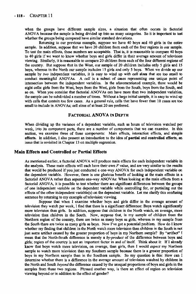
-118 - CHAPTER 11
when the groups have different sample sizes, a situation that often occurs in factorialANOVA because the sample is being divided up into so many categories. So it is important to testwhether the groups being compared have similar standard deviations.
Returning to our previous example, suppose we have 40 boys and 40 girls in the entiresample. In addition, suppose that we have 20 children from each of the four regions in our sample.To test the main effects, these numbers are acceptable. That is, it is reasonable to compare 40 boysto 40 girls if we want to know whether boys and girls differ in their average amount of televisionviewing. Similarly, it is reasonable to compare 20 children from each of the four different regions ofthe country. But suppose that in the West, our sample of 20 children includes only 5 girls and 15boys, whereas in the North our sample includes 15 girls and only 5 boys. When we divide up oursample by two independent variables, it is easy to wind up with cell sizes that are too small toconduct meaningful ANOVAs. A cell is a subset of cases representing one unique point ofintersection between the independent variables. In the aforementioned example, there would beeight cells: girls from the West, boys from the West, girls from the South, boys from the South, andso on. When you consider that factorial ANOVAs can have more than two independent variables,the sample can be subdivided a number of times. Without a large initial sample, it is easy to wind upwith cells that contain too few cases. As a general rule, cells that have fewer than 10 cases are toosmall to include in ANOVAs; cell sizes of at least 20 are preferred.
FACTORIAL ANOVA IN DEPTH
When dividing up the variance of a dependent variable, such as hours of television watched perweek, into its component parts, there are a number of components that we can examine. In thissection, we examine three of these components: Main effects, interaction effects, and simpleeffects. In addition, I also present an introduction to the idea of partial and controlled effects, anissue that is revisited in Chapter 13 on multiple regression.
Main Effects and Controlled or Partial Effects
As mentioned earlier, a factorial ANOVA will produce main effects for each independent variable inthe analysis. These main effects will each have their own F value, and are very similar to the resultsthat would be produced if you just conducted a one-way ANOVA for each independent variable onthe dependent variable. However, there is one glorious benefit of looking at the main effects in afactorial ANOVA rather than separate one-way ANOVAs: When looking at the main effects from afactorial ANOVA, it is possible to test whether there are significant differences between the groupsof one independent variable on the dependent variable while controlling for, or partialing out theeffects of the other independent variable(s) on the dependent variable. Let me clarify this confusingsentence by returning to my example of television viewing.
Suppose that when I examine whether boys and girls differ in the average amount oftelevision they watch per week, I find that there is a significant difference: Boys watch significantlymore television than girls. In addition, suppose that children in the North watch, on average, moretelevision than children in the South. Now, suppose that, in my sample of children from theNorthern region of the country, there are twice as many boys as girls, whereas in my sample fromthe South there are twice as many girls as boys. Now I've got a potential problem. How do I knowwhether my finding that children in the North watch more television than children in the South is notjust some artifact caused by the greater proportion of boys in my Northern sample? By "artifact" Imean that the North-South difference is merely a by-product of the difference between boys andgirls; region of the country is not an important factor in and of itself. Think about it: If I alreadyknow that boys watch more television, on average, than girls, then I would expect my Northernsample to watch more television than my Southern sample because there is a greater proportion ofboys in my Northern sample than in the Southern sample. So my question is this: How can Idetermine whether there is a difference in the average amount of television watched by children inthe North and South beyond the difference caused by the unequal proportions of boys and girls in thesamples from these two regions. Phrased another way, is there an effect of region on televisionviewing beyond or in addition to the effect of gender?
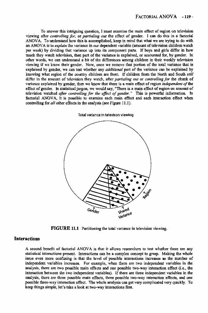
FACTORIAL ANOVA -119 -
To answer this intriguing question, I must examine the main effect of region on televisionviewing after controlling for, or partialing out the effect of gender. I can do this in a factorialANOVA. To understand how this is accomplished, keep in mind that what we are trying to do withan ANOVA is to explain the variance in our dependent variable (amount of television children watchper week) by dividing that variance up into its component parts. If boys and girls differ in howmuch they watch television, then part of the variance is explained, or accounted for, by gender. Inother words, we can understand a bit of the differences among children in their weekly televisionviewing if we know their gender. Now, once we remove that portion of the total variance that isexplained by gender, we can test whether any additional part of the variance can be explained byknowing what region of the country children are from. If children from the North and South stilldiffer in the amount of television they watch, after partialing out or controlling for the chunk ofvariance explained by gender, then we know that there is a main effect of region independent of theeffect of gender. In statistical jargon, we would say, "There is a main effect of region on amount oftelevision watched after controlling for the effect of gender." This is powerful information. Infactorial ANOVA, it is possible to examine each main effect and each interaction effect whencontrolling for all other effects in the analysis (see Figure 11.1).
FIGURE 11.1 Partitioning the total variance in television viewing.
Interactions
A second benefit of factorial ANOVA is that it allows researchers to test whether there are anystatistical interactions present. Interactions can be a complex concept to grasp. Making the wholeissue even more confusing is that the level of possible interactions increases as the number ofindependent variables increases. For example, when there are two independent variables in theanalysis, there are two possible main effects and one possible two-way interaction effect (i.e., theinteraction between the two independent variables). If there are three independent variables in theanalysis, there are three possible main effects, three possible two-way interaction effects, and onepossible three-way interaction effect. The whole analysis can get very complicated very quickly. Tokeep things simple, let's take a look at two-way interactions first.
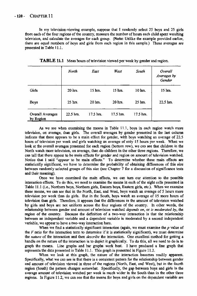
-120 - CHAPTER 11
In my television-viewing example, suppose that I randomly select 25 boys and 25 girlsfrom each of the four regions of the country, measure the number of hours each child spent watchingtelevision, and calculate the averages for each group. (Note: Unlike the example provided earlier,there are equal numbers of boys and girls from each region in this sample.) These averages arepresented in Table 11.1.
TABLE 11.1 Mean hours of television viewed per week by gender and region.
Girls
Boys
Overall Averagesby Region
North
20 hrs.
25 hrs.
22.5 hrs.
East
15 hrs.
20 hrs.
17.5 hrs.
West
15 hrs.
20 hrs.
17.5 hrs.
South
10 hrs.
25 hrs.
17.5 hrs.
OverallAverages by
Gender
15 hrs.
22.5 hrs.
As we see when examining the means in Table 11.1, boys in each region watch moretelevision, on average, than girls. The overall averages by gender presented in the last columnindicate that there appears to be a main effect for gender, with boys watching an average of 22.5hours of television per week and girls watching an average of only 15 hours per week. When welook at the overall averages presented for each region (bottom row), we can see that children in theNorth watch more television, on average, than do children in the other three regions. Therefore, wecan tell that there appear to be main effects for gender and region on amount of television watched.Notice that I said "appear to be main effects." To determine whether these main effects arestatistically significant, we have to determine the probability of obtaining differences of this sizebetween randomly selected groups of this size (see Chapter 7 for a discussion of significance testsand their meaning).
Once we have examined the main effects, we can turn our attention to the possibleinteraction effects. To do this, we need to examine the means in each of the eight cells presented inTable 11.1 (i.e., Northern boys, Northern girls, Eastern boys, Eastern girls, etc.). When we examinethese means, we can see that in the North, East, and West, boys watch an average of 5 hours moretelevision per week than do girls. But in the South, boys watch an average of 15 more hours oftelevision than girls. Therefore, it appears that the differences in the amount of television watchedby girls and boys are not uniform across the four regions of the country. In other words, therelationship between gender and amount of television watched depends on, or is moderated by, theregion of the country. Because the definition of a two-way interaction is that the relationshipbetween an independent variable and a dependent variable is moderated by a second independentvariable, we appear to have a two-way interaction here.
When we find a statistically significant interaction (again, we must examine the p value ofthe F ratio for the interaction term to determine if it is statistically significant), we must determinethe nature of the interaction and then describe the interaction. One excellent method for getting ahandle on the nature of the interaction is to depict it graphically. To do this, all we need to do is tograph the means. Line graphs and bar graphs work best. I have produced a line graph thatrepresents the data presented in Table 11.1. This graph is presented in Figure 11.2.
When we look at this graph, the nature of the interaction becomes readily apparent.Specifically, what we can see is that there is a consistent pattern for the relationship between genderand amount of television viewed in three of the regions (North, East, and West), but in the fourthregion (South) the pattern changes somewhat. Specifically, the gap between boys and girls in theaverage amount of television watched per week is much wider in the South than in the other threeregions. In Figure 11.2, we can see that the means for boys and girls on the dependent variable are
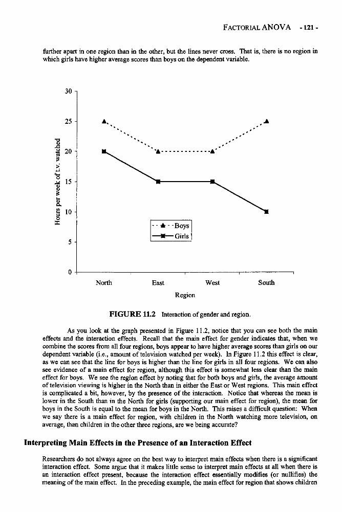
FACTORIAL ANOVA -121 -
further apart in one region than in the other, but the lines never cross. That is, there is no region inwhich girls have higher average scores than boys on the dependent variable.
FIGURE 11.2 Interaction of gender and region.
As you look at the graph presented in Figure 11.2, notice that you can see both the maineffects and the interaction effects. Recall that the main effect for gender indicates that, when wecombine the scores from all four regions, boys appear to have higher average scores than girls on ourdependent variable (i.e., amount of television watched per week). In Figure 11.2 this effect is clear,as we can see that the line for boys is higher than the line for girls in all four regions. We can alsosee evidence of a main effect for region, although this effect is somewhat less clear than the maineffect for boys. We see the region effect by noting that for both boys and girls, the average amountof television viewing is higher in the North than in either the East or West regions. This main effectis complicated a bit, however, by the presence of the interaction. Notice that whereas the mean islower in the South than in the North for girls (supporting our main effect for region), the mean forboys in the South is equal to the mean for boys in the North. This raises a difficult question: Whenwe say there is a main effect for region, with children in the North watching more television, onaverage, than children in the other three regions, are we being accurate?
Interpreting Main Effects in the Presence of an Interaction Effect
Researchers do not always agree on the best way to interpret main effects when there is a significantinteraction effect. Some argue that it makes little sense to interpret main effects at all when there isan interaction effect present, because the interaction effect essentially modifies (or nullifies) themeaning of the main effect. In the preceding example, the main effect for region that shows children
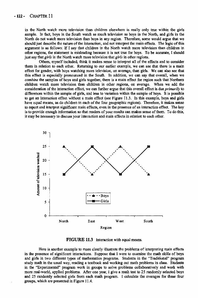
-122 - CHAPTER 11
in the North watch more television than children elsewhere is really only true within the girlssample. In fact, boys in the South watch as much television as boys in the North, and girls in theNorth do not watch more television than boys in any region. Therefore, some would argue that weshould just describe the nature of the interaction, and not interpret the main effects. The logic of thisargument is as follows: If I say that children in the North watch more television than children inother regions, the statement is misleading because it is not true for boys. To be accurate, I shouldjust say that girls in the North watch more television that girls in other regions.
Others, myself included, think it makes sense to interpret all of the effects and to considerthem in relation to each other. Returning to our earlier example, we can see that there is a maineffect for gender, with boys watching more television, on average, than girls. We can also see thatthis effect is especially pronounced in the South. In addition, we can say that overall, when wecombine the samples of boys and girls together, there is a main effect for region such that Northernchildren watch more television than children in other regions, on average. When we add theconsideration of the interaction effect, we can further argue that this overall effect is due primarily todifferences within the sample of girls, and less to variation within the sample of boys. It is possibleto get an interaction effect without a main effect (see Figure 11.3. In this example, boys and girlshave equal means, as do children in each of the four geographic regions). Therefore, it makes senseto report and interpret significant main effects, even in the presence of an interaction effect. The keyis to provide enough information so that readers of your results can makes sense of them. To do this,it may be necessary to discuss your interaction and main effects in relation to each other.
FIGURE 11.3 Interaction with equal means.
Here is another example to more clearly illustrate the problems of interpreting main effectsin the presence of significant interactions. Suppose that I were to examine the math skills of boysand girls in two different types of mathematics programs. Students in the "Traditional" programstudy math in the usual way, reading a textbook and working out math problems in class. Studentsin the "Experimental" program work in groups to solve problems collaboratively and work withmore real-world, applied problems. After one year, I give a math test to 25 randomly selected boysand 25 randomly selected girls from each math program. I calculate the averages for these fourgroups, which are presented in Figure 11.4.
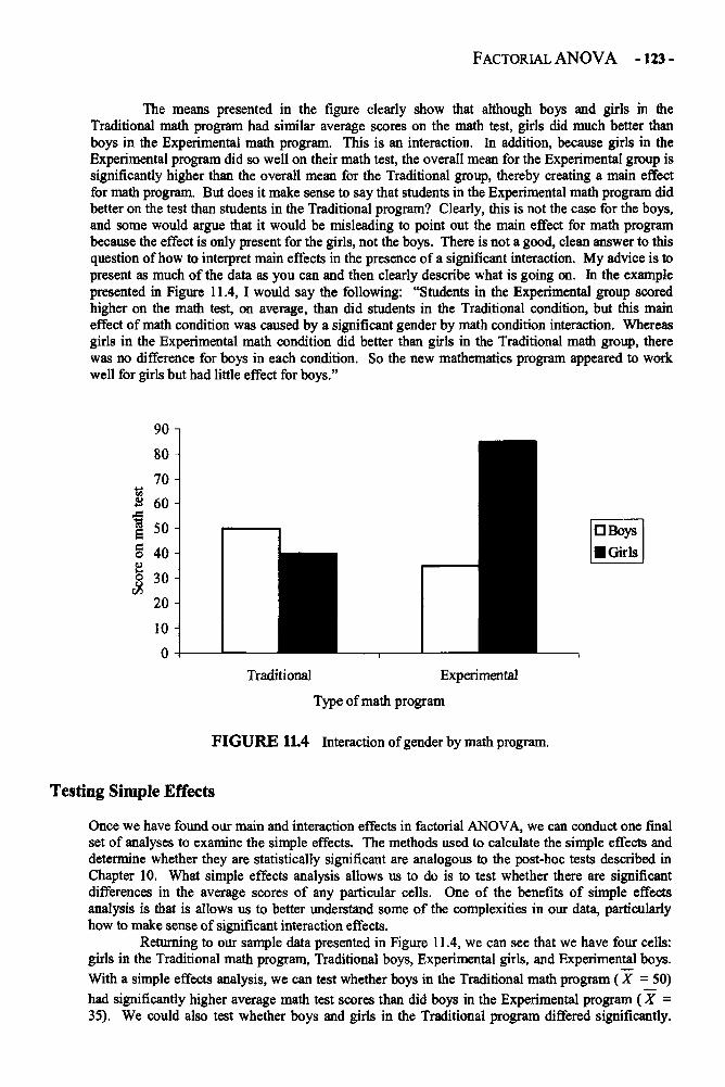
FACTORIAL ANOVA -123 -
The means presented in the figure clearly show that although boys and girls in theTraditional math program had similar average scores on the math test, girls did much better thanboys in the Experimental math program. This is an interaction. In addition, because girls in theExperimental program did so well on their math test, the overall mean for the Experimental group issignificantly higher than the overall mean for the Traditional group, thereby creating a main effectfor math program. But does it make sense to say that students in the Experimental math program didbetter on the test than students in the Traditional program? Clearly, this is not the case for the boys,and some would argue that it would be misleading to point out the main effect for math programbecause the effect is only present for the girls, not the boys. There is not a good, clean answer to thisquestion of how to interpret main effects in the presence of a significant interaction. My advice is topresent as much of the data as you can and then clearly describe what is going on. In the examplepresented in Figure 11.4, I would say the following: "Students in the Experimental group scoredhigher on the math test, on average, than did students in the Traditional condition, but this maineffect of math condition was caused by a significant gender by math condition interaction. Whereasgirls in the Experimental math condition did better than girls in the Traditional math group, therewas no difference for boys in each condition. So the new mathematics program appeared to workwell for girls but had little effect for boys."
Testing Simple Effects
Once we have found our main and interaction effects in factorial ANOVA, we can conduct one finalset of analyses to examine the simple effects. The methods used to calculate the simple effects anddetermine whether they are statistically significant are analogous to the post-hoc tests described inChapter 10. What simple effects analysis allows us to do is to test whether there are significantdifferences in the average scores of any particular cells. One of the benefits of simple effectsanalysis is that is allows us to better understand some of the complexities in our data, particularlyhow to make sense of significant interaction effects.
Returning to our sample data presented in Figure 11.4, we can see that we have four cells:girls in the Traditional math program, Traditional boys, Experimental girls, and Experimental boys.With a simple effects analysis, we can test whether boys in the Traditional math program ( X = 50)had significantly higher average math test scores than did boys in the Experimental program ( X =35). We could also test whether boys and girls in the Traditional program differed significantly.
-124 - CHAPTER 11
Perhaps most important for helping us understand the interaction effect, we can test whether girls inthe Experimental program had higher average math test scores than students in each of the threeother groups. For a detailed description of the methods for calculating simple effects, I recommendreading Hinkle, Wiersma, and Jurs (1998).
Analysis of Covariance
Earlier in this chapter, I suggested that one of the benefits of conducting factorial ANOVAs is that itallows us to determine whether groups differ on some dependent variable while controlling for, orpartialing out, the effects of other independent variables. A closely related concept that applies to alltypes of ANOVA, including one-way, factorial, and repeated-measures, is the use of covariates inthese analyses. In analysis of covariance (ANCOVA), the idea is to test whether there aredifferences between groups on a dependent variable after controlling for the effects of a differentvariable, or set of variables. The difference between an ANCOVA and the types of controlledvariance I described earlier is that with an ANCOVA, the variable(s) that we are controlling for, orpartialing out the effects of, is not necessarily an independent variable. Let me explain.
In my earlier example, I was able to test whether boys and girls differed in the amount oftelevision they watched while controlling for the effects of which region of the country they lived in(the second independent variable), as well as the interaction between the two independent variables.But in an ANCOVA analysis, we can control the effects of variables besides independent variables.For example, I could use socioeconomic status (SES) as a covariate and test whether children indifferent regions of the country differ in the amount of television they watch after partialing out theeffects of their SES. Suppose that my sample of children from the North is less wealthy than mysamples from the three other regions. Suppose further than children from poorer families tend towatch more television than children from wealthier families. Because of this, my earlier results thatfound greater television watching among children in the Northern region may simply be due to thefact that these children are less wealthy than children in the other regions. With ANCOVA, I cantest whether the difference in the viewing habits of children from different regions is due strictly todifferences in SES, or whether there are regional differences independent of the effects of SES. Thisis particularly handy because even though factorial ANOVA only allows us to use categorical (i.e.,nominally scaled) independent variables, with ANCOVA we can also control the effects ofcontinuous (i.e., intervally scaled) variables.
Effect Size
As I did in Chapter 10, I will illustrate effect size in factorial ANOVA, along with some of theparticulars about sums of squares, mean squares, and F values, using output from an analysis of myown data using the SPSS computer software program. In this example, students' confidence in theirability to understand and successfully complete their English classwork, referred to here as "self-efficacy," is the dependent variable. I want to see whether high school boys and girls differ in theirself-efficacy (i.e., a main effect for gender), whether students with relatively high grade pointaverages (GPA) differ from those with relatively low GPAs in their self-efficacy (i.e., a main effectfor GPA), and whether there is an interaction between gender and GPA on self-efficacy. Gender, ofcourse, is a two-category independent variable. To make GPA a two-category variable, I dividestudents into high- and low-GPA groups by splitting the sample in two using the median GPA.Researchers often divide continuous variables into variables with two or three neatly definedcategories (e.g., below the median and above the median; low, middle, and high groups). Thisallows me to perform a 2 (gender) x 2 (GPA) factorial ANOVA. Self-efficacy is measured using asurvey with a 5-point scale (1 = "not at all confident" and 5 = "very confident"). My sampleconsists of 468 high school students.
The results presented in Table 11.2 begin with descriptive statistics. These statistics arepresented separately by subgroups (e.g., low-achieving girls, high-achieving girls, all girlscombined, low-achieving boys, etc.). The means and standard deviations presented are for thedependent variable, self-efficacy. By glancing over the means, we can see that the boys in our
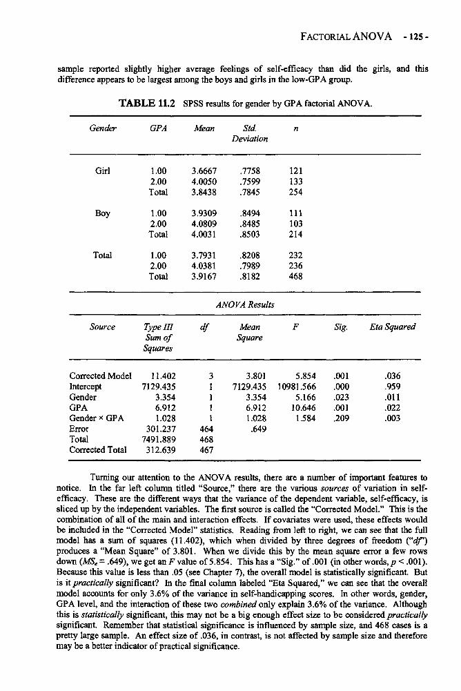
FACTORIAL ANOVA -125 -
sample reported slightly higher average feelings of self-efficacy than did the girls, and thisdifference appears to be largest among the boys and girls in the low-GP A group.
TABLE 11.2 SPSS results for gender by GPA factorial ANOVA.
Gender
Girl
Boy
Total
GPA
1.002.00Total
1.002.00Total
1.002.00Total
Mean
3.66674.00503.8438
3.93094.08094.0031
3.79314.03813.9167
Std.Deviation
.7758
.7599
.7845
.8494
.8485
.8503
.8208
.7989
.8182
n
121133254
111103214
232236468
ANOVA Results
Source
Corrected ModelInterceptGenderGPAGender x GPAErrorTotalCorrected Total
Type IIISum of
Squares
11.4027129.435
3.3546.9121.028
301.2377491.889312.639
df
31111
464468467
MeanSquare
3.8017129.435
3.3546.9121.028.649
F
5.85410981.566
5.16610.646
1.584
Sig.
.001
.000
.023
.001
.209
Eta Squared
.036
.959
.011
.022
.003
Turning our attention to the ANOVA results, there are a number of important features tonotice. In the far left column titled "Source," there are the various sources of variation in self-efficacy. These are the different ways that the variance of the dependent variable, self-efficacy, issliced up by the independent variables. The first source is called the "Corrected Model." This is thecombination of all of the main and interaction effects. If covariates were used, these effects wouldbe included in the "Corrected Model" statistics. Reading from left to right, we can see that the fullmodel has a sum of squares (11.402), which when divided by three degrees of freedom ("df ' )produces a "Mean Square" of 3.801. When we divide this by the mean square error a few rowsdown (MSe = .649), we get an F value of 5.854. This has a "Sig." of .001 (in other words, p < .001).Because this value is less than .05 (see Chapter 7), the overall model is statistically significant. Butis it practically significant? In the final column labeled "Eta Squared," we can see that the overallmodel accounts for only 3.6% of the variance in self-handicapping scores. In other words, gender,GPA level, and the interaction of these two combined only explain 3.6% of the variance. Althoughthis is statistically significant, this may not be a big enough effect size to be considered practicallysignificant. Remember that statistical significance is influenced by sample size, and 468 cases is apretty large sample. An effect size of .036, in contrast, is not affected by sample size and thereforemay be a better indicator of practical significance.
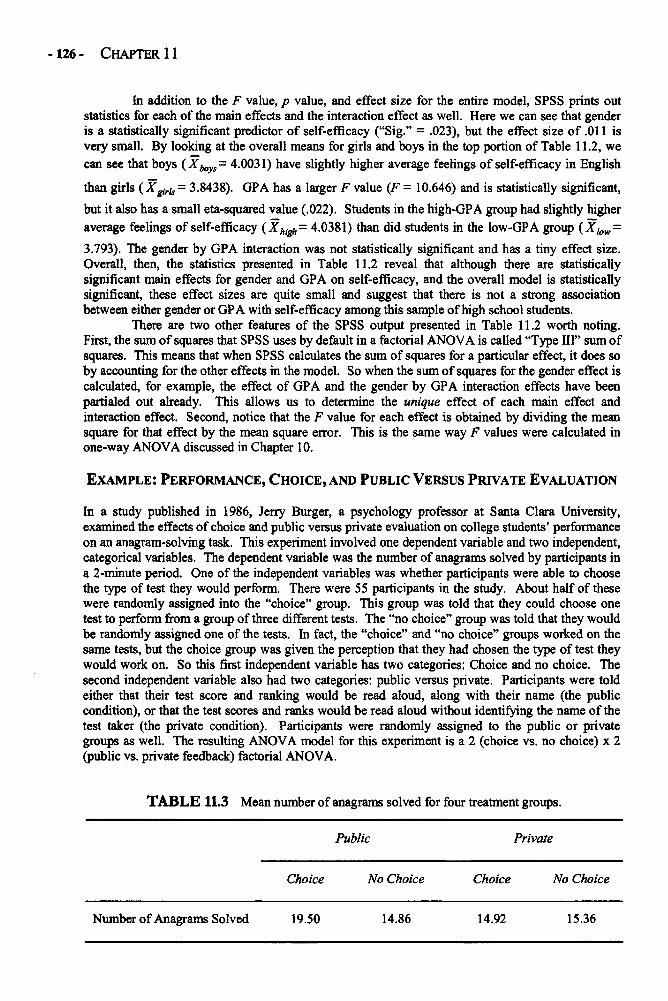
-126- CHAPTER 11
In addition to the F value, p value, and effect size for the entire model, SPSS prints outstatistics for each of the main effects and the interaction effect as well. Here we can see that genderis a statistically significant predictor of self-efficacy ("Sig." = .023), but the effect size of .011 isvery small. By looking at the overall means for girls and boys in the top portion of Table 11.2, wecan see that boys (Xboys 4.0031) have slightly higher average feelings of self-efficacy in English
than girls (X g i r l s = 3.8438). GPA has a larger F value (F = 10.646) and is statistically significant,
but it also has a small eta-squared value (.022). Students in the high-GPA group had slightly higheraverage feelings of self-efficacy (Xhigh= 4.0381) than did students in the low-GPA group (X low =
3.793). The gender by GPA interaction was not statistically significant and has a tiny effect size.Overall, then, the statistics presented in Table 11.2 reveal that although there are statisticallysignificant main effects for gender and GPA on self-efficacy, and the overall model is statisticallysignificant, these effect sizes are quite small and suggest that there is not a strong associationbetween either gender or GPA with self-efficacy among this sample of high school students.
There are two other features of the SPSS output presented in Table 11.2 worth noting.First, the sum of squares that SPSS uses by default in a factorial ANOVA is called "Type III" sum ofsquares. This means that when SPSS calculates the sum of squares for a particular effect, it does soby accounting for the other effects in the model. So when the sum of squares for the gender effect iscalculated, for example, the effect of GPA and the gender by GPA interaction effects have beenpartialed out already. This allows us to determine the unique effect of each main effect andinteraction effect. Second, notice that the F value for each effect is obtained by dividing the meansquare for that effect by the mean square error. This is the same way F values were calculated inone-way ANOVA discussed in Chapter 10.
EXAMPLE: PERFORMANCE, CHOICE, AND PUBLIC VERSUS PRIVATE EVALUATION
In a study published in 1986, Jerry Burger, a psychology professor at Santa Clara University,examined the effects of choice and public versus private evaluation on college students' performanceon an anagram-solving task. This experiment involved one dependent variable and two independent,categorical variables. The dependent variable was the number of anagrams solved by participants ina 2-minute period. One of the independent variables was whether participants were able to choosethe type of test they would perform. There were 55 participants in the study. About half of thesewere randomly assigned into the "choice" group. This group was told that they could choose onetest to perform from a group of three different tests. The "no choice" group was told that they wouldbe randomly assigned one of the tests. In fact, the "choice" and "no choice" groups worked on thesame tests, but the choice group was given the perception that they had chosen the type of test theywould work on. So this first independent variable has two categories: Choice and no choice. Thesecond independent variable also had two categories: public versus private. Participants were toldeither that their test score and ranking would be read aloud, along with their name (the publiccondition), or that the test scores and ranks would be read aloud without identifying the name of thetest taker (the private condition). Participants were randomly assigned to the public or privategroups as well. The resulting ANOVA model for this experiment is a 2 (choice vs. no choice) x 2(public vs. private feedback) factorial ANOVA.
TABLE 11.3 Mean number of anagrams solved for four treatment groups.
Public Private
Choice No Choice Choice No Choice
Number of Anagrams Solved 19.50 14.86 14.92 15.36
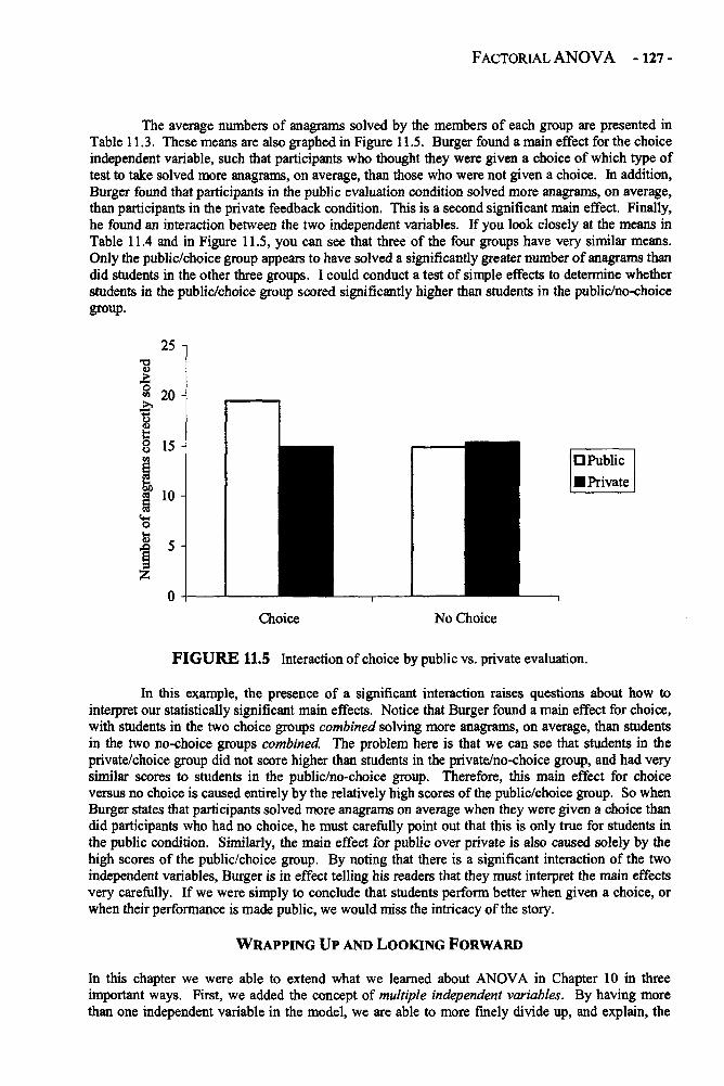
FACTORIAL ANOVA -127 -
The average numbers of anagrams solved by the members of each group are presented inTable 11.3. These means are also graphed in Figure 11.5. Burger found a main effect for the choiceindependent variable, such that participants who thought they were given a choice of which type oftest to take solved more anagrams, on average, than those who were not given a choice. In addition,Burger found that participants in the public evaluation condition solved more anagrams, on average,than participants in the private feedback condition. This is a second significant main effect. Finally,he found an interaction between the two independent variables. If you look closely at the means inTable 11.4 and in Figure 11.5, you can see that three of the four groups have very similar means.Only the public/choice group appears to have solved a significantly greater number of anagrams thandid students in the other three groups. I could conduct a test of simple effects to determine whetherstudents in the public/choice group scored significantly higher than students in the public/no-choicegroup.
FIGURE 11.5 Interaction of choice by public vs. private evaluation.
In this example, the presence of a significant interaction raises questions about how tointerpret our statistically significant main effects. Notice that Burger found a main effect for choice,with students in the two choice groups combined solving more anagrams, on average, than studentsin the two no-choice groups combined The problem here is that we can see that students in theprivate/choice group did not score higher than students in the private/no-choice group, and had verysimilar scores to students in the public/no-choice group. Therefore, this main effect for choiceversus no choice is caused entirely by the relatively high scores of the public/choice group. So whenBurger states that participants solved more anagrams on average when they were given a choice thandid participants who had no choice, he must carefully point out that this is only true for students inthe public condition. Similarly, the main effect for public over private is also caused solely by thehigh scores of the public/choice group. By noting that there is a significant interaction of the twoindependent variables, Burger is in effect telling his readers that they must interpret the main effectsvery carefully. If we were simply to conclude that students perform better when given a choice, orwhen their performance is made public, we would miss the intricacy of the story.
WRAPPING UP AND LOOKING FORWARD
In this chapter we were able to extend what we learned about ANOVA in Chapter 10 in threeimportant ways. First, we added the concept of multiple independent variables. By having morethan one independent variable in the model, we are able to more finely divide up, and explain, the
-128- CHAPTER 11
variance in the dependent variable. Second, we examined the concept of controlling or partialingout the effects of other variables in the model, including covariates, to get a better picture of theunique relation between an independent and a dependent variable. Finally in this chapter, weconsidered the importance of statistical interactions. All three of these concepts provide a hint of theamazing power of many different statistical techniques to explore the relations among variables. Inthe social sciences, as in most fields, variables are related to each other in very complex ways. Welive in a complex world. Although t tests and one-way ANOVA are useful statistical techniques,they are often unable to examine the most interesting questions in the social sciences. It is the messyworld of interactions, shared variance, and multiple predictors that make the statistical life a lifeworth living. So although the concepts in these last few chapters may seem a bit more difficult thanthose discussed earlier in the book, they pay rich dividends when finally understood. In the nextchapter, we enter the complex yet particularly interesting world of repeated-measures ANOVA.
GLOSSARY OF TERMS FOR CHAPTER 11
Analysis of covariance (ANCOVA): An analysis of variance conducted with a covariate. It is ananalysis conducted to test for differences between group means after partialing out thevariance attributable to a covariate.
Cell size: The number of cases in each subgroup of the analysis.Covariate(s): A variable, or group of variables, used to control, or account for, a portion of the
variance in the dependent variable, thus allowing the researcher to test for group differenceswhile controlling for the effects of the covariate.
Factorial ANOVA: An analysis of variance with at least two categorical independent variables.Homogeneity of variance: An assumption of all ANOVA models that there are not statistically
significant differences in the within-group variances on the dependent variable between thegroups being compared.
Interaction (effect): When the relationship between the dependent variable and one independentvariable is moderated by a second independent variable. In other words, when the effect ofone independent variable on the dependent variable differs at various levels of a secondindependent variable.
Main effects: These are the effects for each independent variable on the dependent variable. Inother words, differences between the group means for each independent variable on thedependent variable.
Moderator: When the relationship between the dependent variable and one independent variablediffers according to the level of a second independent variable, the second independentvariable acts as a moderator variable. It is a variable that moderates, or influences, therelationship between a dependent variable and an independent variable.
Partial and controlled effects: When the shared, or explained variance between a dependentvariable and an independent variable (or a covariate) is held constant, thereby allowing theresearcher to examine group differences net of the controlled effects.
Simple effects: The differences between the means of each subgroup in a factorial ANOVA. (Asubgroup involves the division of an independent variable into smaller groups. Forexample, if ethnicity is one independent variable, e.g., African-American, Asian-American,and Hispanic-Latino, and gender is another variable, then each ethnic group has twosubgroups, e.g., African-American females and African American-males.)
RECOMMENDED READING
Iverson, G. R., & Norpoth, H. (1987). Analysis of variance (2nd ed.) Newbury Park, CA:Sage.
Wildt, A. R., & Ahtola, O. T. (1978). Analysis of covariance. Beverly Hills, CA: Sage.Hinkle, D. E., Wiersma, W., & Jurs, S. G. (1998). Applied statistics for the behavioral
sciences (4th ed.). Boston: Houghton Mifflin.
CHAPTER 12
REPEATED-MEASURES ANALYSIS OF VARIANCE
One type of t test discussed in Chapter 9 was the paired t test. One type of study in which a paired ttest would be used is when we have two scores for a single group on a single measure. For example,if we had a group of third-grade students and we gave them a test of their math abilities at thebeginning of the school year and again at the end of the school year, we would have one group (thirdgraders) with two scores on one measure (the math test). In this situation, we could also use arepeated-measures analysis of variance (ANOVA) to test whether students' scores on the mathtest were different at the beginning and end of the academic year.
Repeated-measures ANOVA has a number of advantages over paired t tests, however.First, with repeated-measures ANOVA, we can examine differences on a dependent variable that hasbeen measured at more than two time points, whereas with an independent t test we can onlycompare scores on a dependent variable from two time points. Second, as discussed in Chapter 11on factorial ANOVA, with a repeated-measures ANOVA we can control for the effects of one ormore covariates, thereby conducting a repeated-measures analysis of covariance (ANCOVA). Third,in a repeated-measures ANOVA, we can also include one or more independent categorical, or groupvariables. This type of mixed model is a particularly useful technique and is discussed in somedetail later in the chapter.
When to Use Each Type of Repeated-Measures Technique
The most basic form of a repeated-measures ANOVA occurs when there is a single group (e.g., thirdgraders) with two scores (e.g., beginning of the year, end of the year) on a single dependent variable(e.g., a mathematics test). This is a very common model that is often used in simple laboratoryexperiments. For example, suppose I wanted to know whether drinking alcohol affects the reactiontime of adults when driving. I could take a group of 50 adults and test their stop reaction time byflashing a red light at each one of them when they are driving and measuring how long it takes foreach one to apply the brakes. After calculating the average amount of time it takes this group toapply the brakes when sober, I could then ask each member of my group to consume two alcoholicdrinks and then again test their reaction time when driving, using the same methods. In thisexample, I've got one group (50 adults) with two scores on one dependent variable (reaction timewhen driving). After the second measure of reaction time, I could ask each of my participants toconsume two more alcoholic drinks and again test their reaction time. Now I've got three measuresof reaction time that I can use in my repeated-measures ANOVA. Notice that my dependentvariable is always the same measure (reaction time), and my group is always the same (sample of 50adults). The results of my repeated-measures ANOVA will tell me whether, on average, there aredifferences in reaction time across my three trials. If there are, I might logically conclude thatdrinking alcohol affects reaction time, although there may be other explanations for my results (e.g.,my participants may be getting tired or bored with the experiment, they may be getting used to thetest situation, etc.).
-129-
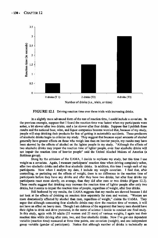
-130- CHAPTER 12
FIGURE 12.1 Driving reaction time over three trials with increasing drinks.
In a slightly more advanced form of the test of reaction time, I could include a covariate. Inthe previous example, suppose that I found the reaction time was fastest when my participants weresober, a bit slower after two drinks, and a lot slower after four drinks. Suppose that I publish theseresults and the national beer, wine, and liquor companies become worried that, because of my study,people will stop drinking their products for fear of getting in automobile accidents. These producersof alcoholic drinks begin to criticize my study. They suggest that because equal amounts of alcoholgenerally have greater effects on those who weigh less than on heavier people, my results may havebeen skewed by the effects of alcohol on the lighter people in my study. "Although the effects oftwo alcoholic drinks may impair the reaction time of lighter people, even four alcoholic drinks willnot impair the reaction time of heavier people" said the United Alcohol Makers of America (afictitious group).
Stung by the criticism of the UAMA, I decide to replicate my study, but this time I useweight as a covariate. Again, I measure participants' reaction time when driving completely sober,after two alcoholic drinks and after four alcoholic drinks. In addition, this time I weigh each of myparticipants. Now when I analyze my data, I include my weight covariate. I find that, aftercontrolling, or partialing out the effects of weight, there is no difference in the reaction time ofparticipants before they have any drinks and after they have two drinks, but after four drinks myparticipants react more slowly, on average, than they did after zero or two drinks (Figure 12.2).These results suggest that drinking may increase the reaction time of lighter people after only twodrinks, but it seems to impair the reaction time of people, regardless of weight, after four drinks.
Still bothered by my results, the UAMA suggests that my results are skewed because I didnot look at the effects of drinking on reaction time separately for men and women. "Women aremore dramatically affected by alcohol than men, regardless of weight," claims the UAMA. Theyargue that although consuming four alcoholic drinks may slow the reaction time of women, it willnot have an effect on heavy men. Though I am dubious of the argument that heavy men should havetheir rights to drink and drive protected, in the name of science I decide to conduct one final study.In this study, again with 50 adults (25 women and 25 men) of various weights, I again test theirreaction time while driving after zero, two, and four alcoholic drinks. Now I've got one dependentvariable (reaction time) measured at three time points, one covariate (weight), and one independentgroup variable (gender of participant). Notice that although number of drinks is technically an
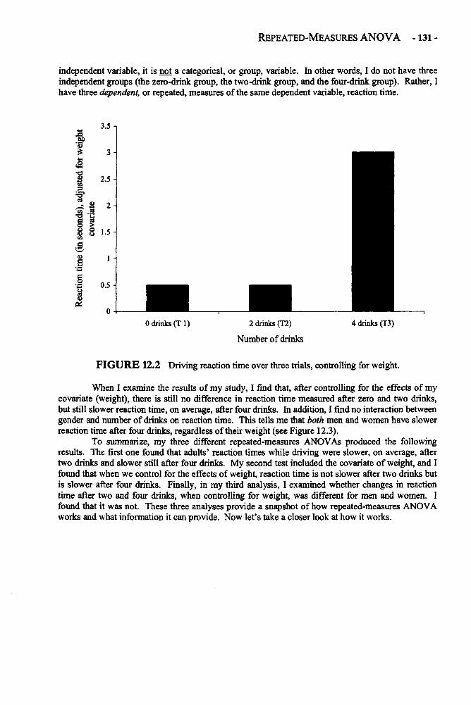
REPEATED-MEASURES ANOVA -131-
independent variable, it is not a categorical, or group, variable. In other words, I do not have threeindependent groups (the zero-drink group, the two-drink group, and the four-drink group). Rather, Ihave three dependent, or repeated, measures of the same dependent variable, reaction time.
FIGURE 12.2 Driving reaction time over three trials, controlling for weight.
When I examine the results of my study, I find that, after controlling for the effects of mycovariate (weight), there is still no difference in reaction time measured after zero and two drinks,but still slower reaction time, on average, after four drinks. In addition, I find no interaction betweengender and number of drinks on reaction time. This tells me that both men and women have slowerreaction time after four drinks, regardless of their weight (see Figure 12.3).
To summarize, my three different repeated-measures ANOVAs produced the followingresults. The first one found that adults' reaction times while driving were slower, on average, aftertwo drinks and slower still after four drinks. My second test included the covariate of weight, and Ifound that when we control for the effects of weight, reaction time is not slower after two drinks butis slower after four drinks. Finally, in my third analysis, I examined whether changes in reactiontime after two and four drinks, when controlling for weight, was different for men and women. Ifound that it was not. These three analyses provide a snapshot of how repeated-measures ANOVAworks and what information it can provide. Now let's take a closer look at how it works.
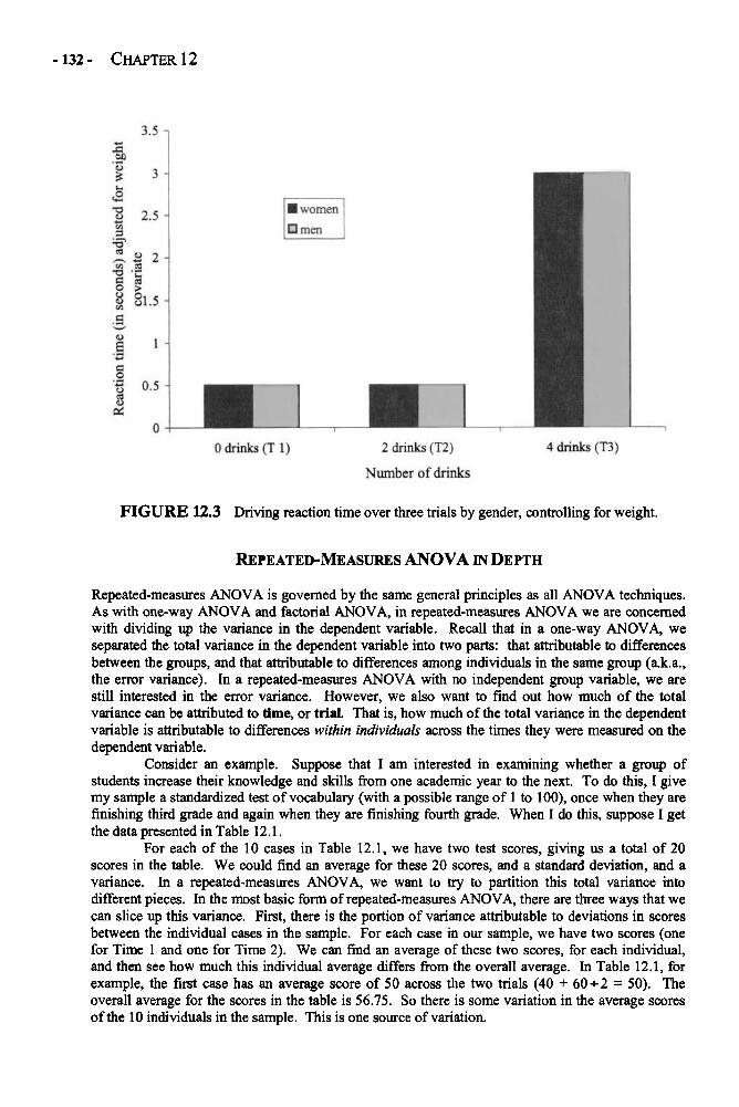
-132- CHAPTER 12
FIGURE 12.3 Driving reaction time over three trials by gender, controlling for weight.
REPEATED-MEASURES ANOVA IN DEPTH
Repeated-measures ANOVA is governed by the same general principles as all ANOVA techniques.As with one-way ANOVA and factorial ANOVA, in repeated-measures ANOVA we are concernedwith dividing up the variance in the dependent variable. Recall that in a one-way ANOVA, weseparated the total variance in the dependent variable into two parts: that attributable to differencesbetween the groups, and that attributable to differences among individuals in the same group (a.k.a.,the error variance). In a repeated-measures ANOVA with no independent group variable, we arestill interested in the error variance. However, we also want to find out how much of the totalvariance can be attributed to time, or trial. That is, how much of the total variance in the dependentvariable is attributable to differences within individuals across the times they were measured on thedependent variable.
Consider an example. Suppose that I am interested in examining whether a group ofstudents increase their knowledge and skills from one academic year to the next. To do this, I givemy sample a standardized test of vocabulary (with a possible range of 1 to 100), once when they arefinishing third grade and again when they are finishing fourth grade. When I do this, suppose I getthe data presented in Table 12.1.
For each of the 10 cases in Table 12.1, we have two test scores, giving us a total of 20scores in the table. We could find an average for these 20 scores, and a standard deviation, and avariance. In a repeated-measures ANOVA, we want to try to partition this total variance intodifferent pieces. In the most basic form of repeated-measures ANOVA, there are three ways that wecan slice up this variance. First, there is the portion of variance attributable to deviations in scoresbetween the individual cases in the sample. For each case in our sample, we have two scores (onefor Time 1 and one for Time 2). We can find an average of these two scores, for each individual,and then see how much this individual average differs from the overall average. In Table 12.1, forexample, the first case has an average score of 50 across the two trials (40 + 60 + 2 = 50). Theoverall average for the scores in the table is 56.75. So there is some variation in the average scoresof the 10 individuals in the sample. This is one source of variation.

REPEATED-MEASURES ANOVA -133 -
TABLE 12.1 Vocabulary test scores at two time points.
Case Number Test Score, Time 1 (Third Grade) Test Score, Time 2 (Fourth Grade)
1
2
3
4
5
6
7
8
9
10
Trial (or Time)Average
40
55
60
40
75
80
65
40
20
45
X=51.5
60
55
70
45
70
85
75
60
35
60
X=61.6
The second source of variation in the scores involves the within-subject variance, ordifferences, between Time 1 and Time 2 scores. As we can see by looking at the scores in Table12.1 and in Figure 12.4, it appears that students generally had different scores on the test at Time 1than they did at Time 2. These intra-individual, or within-subject, differences between Time 1 andTime 2 scores can be seen more easily in the graph presented in Figure 12.4. These intra-individualchanges reflect differences, or variance, within each individual, and therefore are called within-subject effects. What we are interested in is whether, on average, individuals' scores were differentat Time 1 (in third grade) than they were at Time 2 (in fourth grade). Notice that we are askingwhether there were differences in the scores between Time 1 and Time 2 on average. If the scoresof some of the cases went up from Time 1 to Time 2, but the scores of other cases went down by thesame amount, then these changes would cancel each other out, and there would be no averagedifference between the Time 1 and Time 2 scores. But if the scores either went up or down onaverage between Time 1 and Time 2, then we could say that some of the total variation can beattributable to within-subject differences across time. A look at the scores in Table 12.1 and Figure12.4 reveals that scores appear to increase from Time 1 to Time 2. To examine whether there aredifferences in the average scores across time, all we need to do is calculate the average score at eachtime and find the difference between these average scores and the overall average. In the precedingparagraph, we found that the overall average score was 56.75. In Table 12.1, we can see that theaverage for Time 1 is 51.5, and the average score for Time 2 is 61.5. So we can see that there issome variance in the average scores at the two times (i.e., third and fourth grade), suggesting thatthere may be a within-subjects effect.
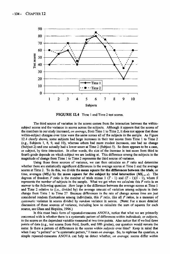
-134- CHAPTER 12
FIGURE 12.4 Time 1 and Time 2 test scores.
The third source of variation in the scores comes from the interaction between the within-subject scores and the variance in scores across the subjects. Although it appears that the scores ofthe members in our study increased, on average, from Time 1 to Time 2, it does not appear that thesewithin-subject changes over time were the same across all of the subjects in the sample. As Figure12.4 clearly shows, some subjects had large increases in their test scores from Time 1 to Time 2(e.g., Subjects 1, 8, 9, and 10), whereas others had more modest increases, one had no change(Subject 2) and one actually had a lower score at Time 2 (Subject 5). So there appears to be a case,or subject, by time interaction. In other words, the size of the increase in test score from third tofourth grade depends on which subject we are looking at. This difference among the subjects in themagnitude of change from Time 1 to Time 2 represents the third source of variance.
Using these three sources of variance, we can then calculate an F ratio and determinewhether there are statistically significant differences in the average scores at Time 1 and the averagescores at Time 2. To do this, we divide the mean square for the differences between the trials, ortime, averages (MST) by the mean square for the subject by trial interaction (MSS x T). Thedegrees of freedom F ratio is the number of trials minus 1 (T - 1) and (T - 1)(S - 1), where Srepresents the number of subjects in the sample. What we get when we calculate this F ratio is ananswer to the following question: How large is the difference between the average scores at Time 1and Time 2 relative to (i.e., divided by) the average amount of variation among subjects in theirchange from Time 1 to Time 2? Because differences in the rate of change across time are justconsidered random fluctuations among individuals, this F ratio, like all F ratios, is a measure ofsystematic variance in scores divided by random variance in scores. (Note: For a more detaileddiscussion of these sources of variance, including how to calculate the sum of squares for eachsource, see Glass and Hopkins, 1996.)
In this most basic form of repeated-measures ANOVA, notice that what we are primarilyconcerned with is whether there is a systematic pattern of differences within individuals, or subjects,in the scores on the dependent variable measured at two time points. Also notice that if we had threepoints of data (e.g., test scores from third, fourth, and fifth grades), our question would remain thesame: Is there a pattern of differences in the scores within subjects over time? Keep in mind thatwhen I say "a pattern" or "a systematic pattern," I mean on average. So, to rephrase the question, asimple repeated-measures ANOVA can help us detect whether, on average, scores differ within
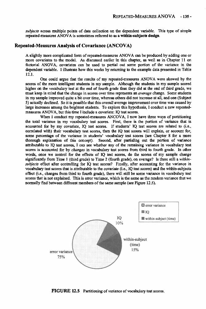
REPEATED-MEASURES ANOVA -135 -
subjects across multiple points of data collection on the dependent variable. This type of simplerepeated-measures ANOVA is sometimes referred to as a within-subjects design.
Repeated-Measures Analysis of Covariance (ANCOVA)
A slightly more complicated form of repeated-measures ANOVA can be produced by adding one ormore covariates to the model. As discussed earlier in this chapter, as well as in Chapter 11 onfactorial ANOVA, covariates can be used to partial out some portion of the variance in thedependent variable. I illustrate how this works by returning to the example data presented in Table12.1.
One could argue that the results of my repeated-measures ANOVA were skewed by thescores of the more intelligent students in my sample. Although the students in my sample scoredhigher on the vocabulary test at the end of fourth grade than they did at the end of third grade, wemust keep in mind that the change in scores over time represents an average change. Some studentsin my sample improved quite a bit over time, whereas others did not increase at all, and one (Subject5) actually declined. So it is possible that this overall average improvement over time was caused bylarge increases among the brightest students. To explore this hypothesis, I conduct a new repeated-measures ANOVA, but this time I include a covariate: IQ test scores.
When I conduct my repeated-measures ANCOVA, I now have three ways of partitioningthe total variance in my vocabulary test scores. First, there is the portion of variance that isaccounted for by my covariate, IQ test scores. If students' IQ test scores are related to (i.e.,correlated with) their vocabulary test scores, then the IQ test scores will explain, or account for,some percentage of the variance in students' vocabulary test scores (see Chapter 8 for a morethorough explanation of this concept). Second, after partialing out the portion of varianceattributable to IQ test scores, I can see whether any of the remaining variance in vocabulary testscores is accounted for by changes in vocabulary test scores from third to fourth grade. In otherwords, once we control for the effects of IQ test scores, do the scores of my sample changesignificantly from Time 1 (third grade) to Time 2 (fourth grade), on average? Is there still a within-subjects effect after controlling for IQ test scores? Finally, after accounting for the variance invocabulary test scores that is attributable to the covariate (i.e., IQ test scores) and the within-subjectseffect (i.e., changes from third to fourth grade), there will still be some variance in vocabulary testscores that is not explained. This is error variance, which is the same as the random variance that wenormally find between different members of the same sample (see Figure 12.5).
FIGURE 12.5 Partitioning of variance of vocabulary test scores.
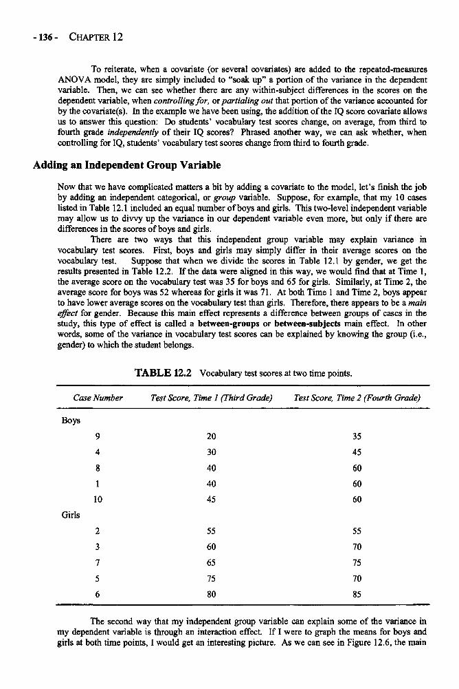
-136- CHAPTER 12
To reiterate, when a covariate (or several covariates) are added to the repeated-measuresANOVA model, they are simply included to "soak up" a portion of the variance in the dependentvariable. Then, we can see whether there are any within-subject differences in the scores on thedependent variable, when controlling for, or partialing out that portion of the variance accounted forby the covariate(s). In the example we have been using, the addition of the IQ score covariate allowsus to answer this question: Do students' vocabulary test scores change, on average, from third tofourth grade independently of their IQ scores? Phrased another way, we can ask whether, whencontrolling for IQ, students' vocabulary test scores change from third to fourth grade.
Adding an Independent Group Variable
Now that we have complicated matters a bit by adding a covariate to the model, let's finish the jobby adding an independent categorical, or group variable. Suppose, for example, that my 10 caseslisted in Table 12.1 included an equal number of boys and girls. This two-level independent variablemay allow us to divvy up the variance in our dependent variable even more, but only if there aredifferences in the scores of boys and girls.
There are two ways that this independent group variable may explain variance invocabulary test scores. First, boys and girls may simply differ in their average scores on thevocabulary test. Suppose that when we divide the scores in Table 12.1 by gender, we get theresults presented in Table 12.2. If the data were aligned in this way, we would find that at Time 1,the average score on the vocabulary test was 35 for boys and 65 for girls. Similarly, at Time 2, theaverage score for boys was 52 whereas for girls it was 71. At both Time 1 and Time 2, boys appearto have lower average scores on the vocabulary test than girls. Therefore, there appears to be a maineffect for gender. Because this main effect represents a difference between groups of cases in thestudy, this type of effect is called a between-groups or between-subjects main effect. In otherwords, some of the variance in vocabulary test scores can be explained by knowing the group (i.e.,gender) to which the student belongs.
TABLE 12.2 Vocabulary test scores at two time points.
Case Number Test Score, Time 1 (Third Grade) Test Score, Time 2 (Fourth Grade)
Boys
9 20 35
4 30 45
8 40 60
1 40 60
10 45 60
Girls
2 55
3 60
7 65
5 75
6 80
55
70
75
70
85
The second way that my independent group variable can explain some of the variance inmy dependent variable is through an interaction effect. If I were to graph the means for boys andgirls at both time points, I would get an interesting picture. As we can see in Figure 12.6, the main

REPEATED-MEASURES ANOVA -137-
effect for gender is clear. In addition, it is also clear that there is a within-subject effect, becauseboth boys and girls have higher scores at Time 2 than they did at Time 1.
FIGURE 12.6 Gender by time interaction.
But what also becomes clear in Figure 12.6 is that the amount of change from Time 1 toTime 2 appears to be greater for boys than for girls. Whereas the average score for girls increased 6points from third to fourth grade, it grew 17 points for boys. These different amounts of changerepresent another source of explained variance in vocabulary test scores: the interaction of thewithin-subjects effect with the between-subjects effect. In other words, there appears to be a gender(i.e., between-subjects) by time (i.e., within-subjects) interaction on vocabulary test scores. Notethat questions about how to interpret the main effect in the presence of a statistically significantinteraction arise here, just as they did in our discussions of interactions in factorial ANOVAs(Chapter 11). In our current example, the main, within-subjects effect for time (i.e., that test scoreswent up from Time 1 to Time 2) may be due primarily to the large increase in scores for boys. So itmay be misleading to say simply that students' scores increase with time (i.e., the main effect)without also noting that the time by gender interaction reveals a large increase for boys but only amodest increase for girls in test scores over time.
To summarize, our final model has a number of effects, each of which can explain some ofthe variance in the vocabulary test scores of the cases in my sample. First, some of the variance invocabulary test scores can be explained by students' IQ test scores. On average, students withhigher IQ test scores had higher vocabulary test scores. Second, even after controlling for IQ, therewas a within-subjects main effect. That is, I can know something about students' scores on thevocabulary test by knowing whether we are talking about Time 1 or Time 2 test scores because, onaverage, students had higher scores at Time 2. Third, there was a between-subjects effect for gender,so I can explain some of the variance in vocabulary test scores by knowing the gender of the student.Girls had higher scores, on average, than did boys. Fourth, my time by gender interaction explainssome additional variance in vocabulary test scores. Although both boys' and girls' scores improvedover time, this improvement was more dramatic among boys, on average. Finally, there is somevariance in vocabulary test scores that I cannot explain with my covariate, time, gender, orinteraction effects: This is error variance (see Figure 12.7).
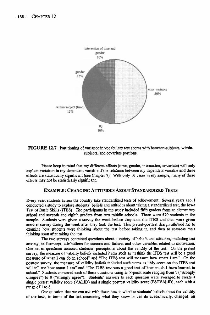
-138- CHAPTER 12
FIGURE 12.7 Partitioning of variance in vocabulary test scores with between-subjects, within-subjects, and covariate portions.
Please keep in mind that my different effects (time, gender, interaction, covariate) will onlyexplain variation in my dependent variable if the relations between my dependent variable and theseeffects are statistically significant (see Chapter 7). With only 10 cases in my sample, many of theseeffects may not be statistically significant.
EXAMPLE: CHANGING ATTITUDES ABOUT STANDARDIZED TESTS
Every year, students across the country take standardized tests of achievement. Several years ago, Iconducted a study to explore students' beliefs and attitudes about taking a standardized test, the IowaTest of Basic Skills (ITBS). The participants in the study included fifth graders from an elementaryschool and seventh and eighth graders from two middle schools. There were 570 students in thesample. Students were given a survey the week before they took the ITBS and then were givenanother survey during the week after they took the test. This pretest-posttest design allowed me toexamine how students were thinking about the test before taking it, and then to reassess theirthinking soon after taking the test.
The two surveys contained questions about a variety of beliefs and attitudes, including testanxiety, self-concept, attributions for success and failure, and other variables related to motivation.One set of questions assessed students' perceptions about the validity of the test. On the pretestsurvey, the measure of validity beliefs included items such as "I think the ITBS test will be a goodmeasure of what I can do in school" and "The ITBS test will measure how smart I am." On theposttest survey, the measure of validity beliefs included such items as "My score on the ITBS testwill tell me how smart I am" and "The ITBS test was a good test of how much I have learned inschool." Students answered each of these questions using an 8-point scale ranging from 1 ("stronglydisagree") to 8 ("strongly agree"). Students' answers to each question were averaged to create asingle pretest validity score (VALID) and a single posttest validity score (PSTVALID), each with arange of 1 to 8.
One question that we can ask with these data is whether students' beliefs about the validityof the tests, in terms of the test measuring what they know or can do academically, changed, on
REPEATED-MEASURES ANOVA -139 -
average, from before they took the test to after. Students may develop a set of beliefs about the testbefore they take it, perhaps due to what their teachers and school administrators tell them inpreparation for the test. But once they take the test, and see what sorts of questions the test contains,they may change their beliefs about what the test really measures. This is a within-subjects type ofquestion: Are there changes within individuals in attitudes about the validity of the test from Time 1to Time 2?
One factor that may cause students to change their attitudes about the validity of the ITBStest is how well they performed on the test. When taking the test, those who thought the test wasdifficult, and knew that they were not doing well on it, may develop a somewhat defensiveperception that the tests are unfair or invalid. On the other hand, those who felt the test was easy andknew they were doing well when taking the test may tend to develop self-augmenting perceptions ofthe test, such as the test reveals their intelligence and is a valid measure. To control for theseperformance-based differences in perceptions of test validity, I add two covariates to the model, bothmeasures of actual test performance. One covariate is the students' scores, in percentile terms, onthe math portion of the ITBS test. The other covariate is students' percentile scores on the verbalportion of the test. The addition of these two variables turns my repeated-measures ANOVA into arepeated-measures ANCOVA. This repeated-measures ANCOVA can be used to answer thefollowing question: When controlling for actual achievement on the test, are there changes withinindividuals in students' attitudes about the validity of the test from Time 1 to Time 2?
Finally, it is possible that boys' and girls' perceptions of the validity of the test may differ.Perhaps one gender is more trusting of standardized measures than the other. In addition, perhapsone gender tends to have more idealized perceptions of the tests' validity before taking the test, butthese perceptions change after actually taking the test. The other gender, with no such idealizedpreconceptions, may not change their attitudes after taking the test. By adding the independentgroup variable of gender, I can now address all of the following questions with my model:
1. When controlling for the effects of gender and achievement, are there changeswithin subjects in students' attitudes about the validity of the test from Time 1to Time 2?
2. When controlling for within-subject effects and achievement, are theredifferences between boys' and girls' average beliefs about the validity of thetest (i.e., between-subjects effects)?
3. Is there a within-subject by between-subject interaction, such that the size ofthe change in perceptions about the validity of the tests from Time 1 to Time 2is different for boys and girls, when controlling for the effects of achievement?
As you can see, there are a number of very interesting questions that I can examine in asingle repeated-measures ANCOVA. To examine these questions, I conducted my analysis usingSPSS software. The actual SPSS output from the analysis is presented in Table 12.3. I explain eachpiece of information in the order it appears in Table 12.3.
The first set of information in Table 12.3 shows the means, standard deviations, and samplesizes for the pretest dependent variable (Pretest Validity) and the posttest dependent variable(Posttest Validity). A quick glance at the separate means for boys and girls on the Pretest Validityand Posttest Validity variables reveals that whereas the girls' averages are virtually identical fromTime 1 to Time 2, the boys' mean declines somewhat (from 6.2852 to 6.0076). We can also see thatat both Time 1 and Time 2, boys appear to score higher, on average, than girls on the validityperception measures (see Figure 12.8). Whether these differences are statistically significant is stillto be determined. Regardless of whether these differences are statistically significant, they may notbe practically significant: Boys and girls do not appear to differ much in their average perceptions ofthe validity of the ITBS test.
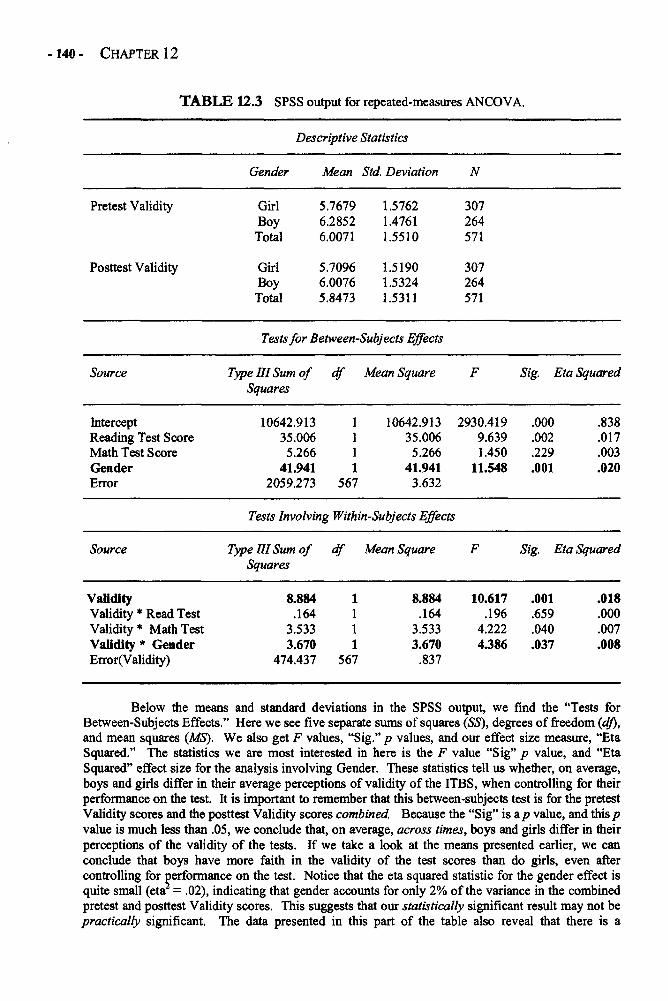
-140- CHAPTER 12
TABLE 12.3 SPSS output for repeated-measures ANCOVA.
Descriptive Statistics
Gender Mean Std. Deviation N
Pretest Validity
Posttest Validity
Girl 5.7679 1.5762Boy 6.2852 1.4761Total 6.0071 1.5510
Girl 5.7096 1.5190Boy 6.0076 1.5324Total 5.8473 1.5311
307264571
307264571
Tests for Between-Subjects Effects
Source
InterceptReading Test ScoreMath Test ScoreGenderError
Type III Sum of df Mean SquareSquares
10642.913 1 10642.91335.006 1 35.0065.266 1 5.266
41.941 1 41.9412059.273 567 3.632
F
2930.4199.6391.450
11.548
Sig. Eta Squared
.000 .838
.002 .017
.229 .003
.001 .020
ValidityValidity * Read TestValidity* Math TestValidity * GenderError(Validity)
8.884.164
3.5333.670
474.437
1111
567
8.884.164
3.5333.670
.837
10.617.196
4.2224.386
.001
.659
.040
.037
.018
.000
.007
.008
Below the means and standard deviations in the SPSS output, we find the "Tests forBetween-Subjects Effects." Here we see five separate sums of squares (55), degrees of freedom (df),and mean squares (MS). We also get F values, "Sig." p values, and our effect size measure, "EtaSquared." The statistics we are most interested in here is the F value "Sig" p value, and "EtaSquared" effect size for the analysis involving Gender. These statistics tell us whether, on average,boys and girls differ in their average perceptions of validity of the ITBS, when controlling for theirperformance on the test. It is important to remember that this between-subjects test is for the pretestValidity scores and the posttest Validity scores combined. Because the "Sig" is a p value, and this pvalue is much less than .05, we conclude that, on average, across times, boys and girls differ in theirperceptions of the validity of the tests. If we take a look at the means presented earlier, we canconclude that boys have more faith in the validity of the test scores than do girls, even aftercontrolling for performance on the test. Notice that the eta squared statistic for the gender effect isquite small (eta2 = .02), indicating that gender accounts for only 2% of the variance in the combinedpretest and posttest Validity scores. This suggests that our statistically significant result may not bepractically significant. The data presented in this part of the table also reveal that there is a
Tests Involving Within-Subjects Effects
Source Type III Sum of df Mean Square F Sig. Eta SquaredSquares
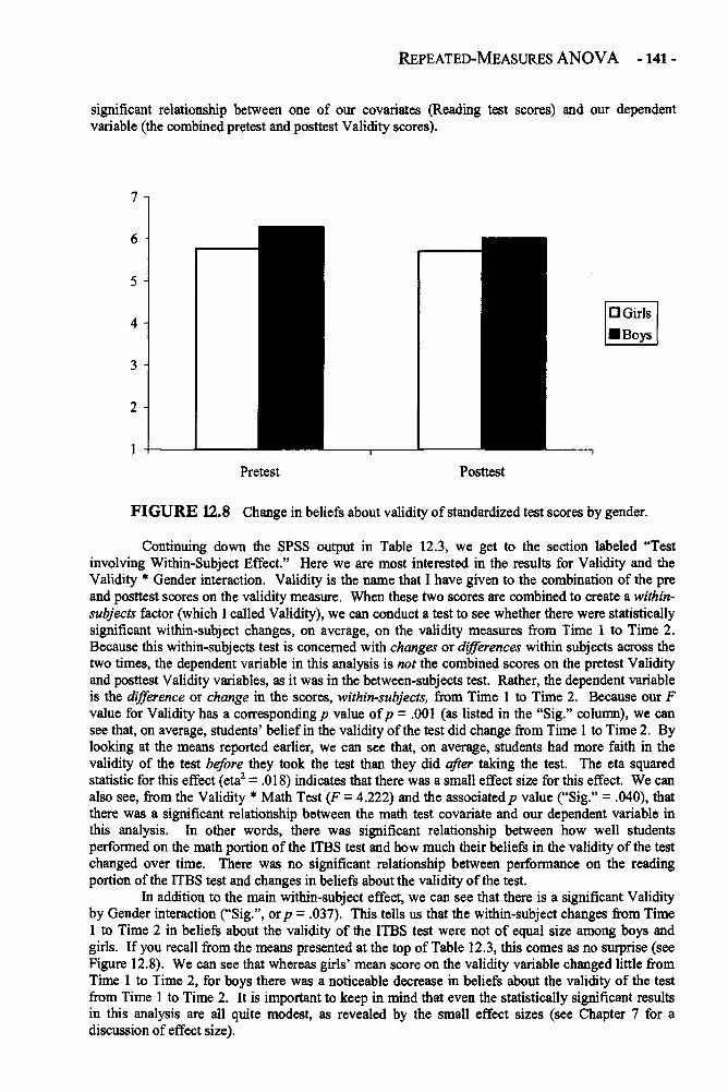
REPEATED-MEASURES ANOVA -141 -
significant relationship between one of our covariates (Reading test scores) and our dependentvariable (the combined pretest and posttest Validity scores).
FIGURE 12.8 Change in beliefs about validity of standardized test scores by gender.
Continuing down the SPSS output in Table 12.3, we get to the section labeled "Testinvolving Within-Subject Effect." Here we are most interested in the results for Validity and theValidity * Gender interaction. Validity is the name that I have given to the combination of the preand posttest scores on the validity measure. When these two scores are combined to create a within-subjects factor (which I called Validity), we can conduct a test to see whether there were statisticallysignificant within-subject changes, on average, on the validity measures from Time 1 to Time 2.Because this within-subjects test is concerned with changes or differences within subjects across thetwo times, the dependent variable in this analysis is not the combined scores on the pretest Validityand posttest Validity variables, as it was in the between-subjects test. Rather, the dependent variableis the difference or change in the scores, within-subjects, from Time 1 to Time 2. Because our Fvalue for Validity has a corresponding p value of p = .001 (as listed in the "Sig." column), we cansee that, on average, students' belief in the validity of the test did change from Time 1 to Time 2. Bylooking at the means reported earlier, we can see that, on average, students had more faith in thevalidity of the test before they took the test than they did after taking the test. The eta squaredstatistic for this effect (eta2 = .018) indicates that there was a small effect size for this effect. We canalso see, from the Validity * Math Test (F = 4.222) and the associated p value ("Sig." = .040), thatthere was a significant relationship between the math test covariate and our dependent variable inthis analysis. In other words, there was significant relationship between how well studentsperformed on the math portion of the ITBS test and how much their beliefs in the validity of the testchanged over time. There was no significant relationship between performance on the readingportion of the ITBS test and changes in beliefs about the validity of the test.
In addition to the main within-subject effect, we can see that there is a significant Validityby Gender interaction ("Sig.", or p = .037). This tells us that the within-subject changes from Time1 to Time 2 in beliefs about the validity of the ITBS test were not of equal size among boys andgirls. If you recall from the means presented at the top of Table 12.3, this comes as no surprise (seeFigure 12.8). We can see that whereas girls' mean score on the validity variable changed little fromTime 1 to Time 2, for boys there was a noticeable decrease in beliefs about the validity of the testfrom Time 1 to Time 2. It is important to keep in mind that even the statistically significant resultsin this analysis are all quite modest, as revealed by the small effect sizes (see Chapter 7 for adiscussion of effect size).
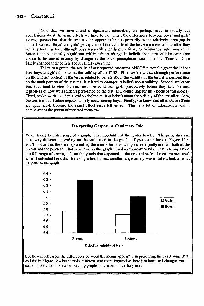
-142- CHAPTER 12
Now that we have found a significant interaction, we perhaps need to modify ourconclusions about the main effects we have found. First, the differences between boys' and girls'average perceptions that the test is valid appear to be due primarily to the relatively large gap inTime 1 scores. Boys' and girls' perceptions of the validity of the test were more similar after theyactually took the test, although boys were still slightly more likely to believe the tests were valid.Second, the statistically significant within-subject change in beliefs about test validity over timeappear to be caused entirely by changes in the boys' perceptions from Time 1 to Time 2. Girlsbarely changed their beliefs about validity over time.
Taken as a group, the results of our repeated-measures ANCOVA reveal a great deal abouthow boys and girls think about the validity of the ITBS. First, we know that although performanceon the English portion of the test is related to beliefs about the validity of the test, it is performanceon the math portion of the test that is related to changes in beliefs about validity. Second, we knowthat boys tend to view the tests as more valid than girls, particularly before they take the test,regardless of how well students performed on the test (i.e., controlling for the effects of test scores).Third, we know that students tend to decline in their beliefs about the validity of the test after takingthe test, but this decline appears to only occur among boys. Finally, we know that all of these effectsare quite small because the small effect sizes tell us so. This is a lot of information, and itdemonstrates the power of repeated measures.
Interpreting Graphs: A Cautionary Tale
When trying to make sense of a graph, it is important that the reader beware. The same data canlook very different depending on the scale used in the graph. If you take a look at Figure 12.8,you'll notice that the bars representing the means for boys and girls look pretty similar, both at thepretest and the posttest. That is because in that graph I used an "honest" y-axis. That is to say I usedthe full range of scores, 1-7, on the y-axis that appeared in the original scale of measurement usedwhen I collected the data. By using a less honest, smaller range on my y-axis, take a look at whathappens to the graph:
See how much larger the differences between the means appear? I'm presenting the exact same dataas I did in Figure 12.8 but it looks different, and more impressive, here just because I changed thescale on the y-axis. So when reading graphs, pay attention to the y-axis.

REPEATED-MEASURES ANOVA -143 -
WRAPPING UP AND LOOKING FORWARD
In some ways, repeated-measures ANOVA is a simple extension of ideas we have already discussed.The similarities with paired t tests (Chapter 9) are clear, as is the idea of parsing up the variance of adependent variable into various components. But the tremendous power of repeated-measuresANOVA can only be appreciated when we take a moment to consider all of the pieces ofinformation that we can gain from a single analysis. The combination of within-subjects andbetween-subjects variance, along with the interaction between these components, allows socialscientists to examine a range of very complex, and very interesting, questions. Repeated-measuresANOVA is a particularly useful technique for examining change over time, either in longitudinalstudies or in experimental studies using a pretreatment, posttreatment design. It is also particularlyuseful for examining whether patterns of change over time vary for different groups.
In the final chapter of the book, we will examine one of the most widely used and versatilestatistical techniques: regression. As you finish this chapter and move onto the next, it is importantto remember that we are only able to scratch the surface of the powerful techniques presented in thelast three chapters of this book. To gain a full appreciation of what factorial ANOVA, repeated-measures ANOVA, and regression can do, you will need to read more about these techniques.
GLOSSARY OF TERMS AND SYMBOLS FOR CHAPTER 12
Between-subjects effect: Differences attributable to variance among the scores on the dependentvariable for individual cases in the ANOVA model.
Between-groups effect: Differences in the average scores for different groups in the ANOVAmodel.
Group variable(s): Categorical independent variable(s) in the ANOVA model.Mean square for the differences between the trials: The average squared deviation between the
participants' average across all trials and their scores on each trial.Mean square for the subject by trial interaction: The average squared deviation between each
individual's change in scores across trials and the average change in scores across trials.Repeated-measures analysis of variance (ANOVA): A statistical technique used to examine
whether the average scores on a dependent variable change over time or trials (i.e., whenmeasured repeatedly).
Time, trial: Each time for which data are collected on the dependent variable.Within-subject variance: Differences within each individual case on scores on the dependent
variable across trials.Within-subjects design: A repeated-measures ANOVA design in which intra-individual changes
across trials are tested. This technique allows the researcher to test whether, on average,individuals score differently at one time than another.
MSS x T: Mean square for the interaction of subject by trial.MST : Mean square for the differences between the trials.
RECOMMENDED READING
Glass, G. V., & Hopkins, K. D. (1996). Statistical methods in education and psychology (3rded.). Boston: Allyn & Bacon.
Marascuilo, L. A., & Serlin, R. C. (1988). Statistical methods for the social and behavioralsciences. New York: Freeman.

This page intentionally left blank
CHAPTER 13
REGRESSION
In Chapter 8, the concept of correlation was introduced. Correlation involves a measure of thedegree to which two variables are related to each other. A closely related concept, coefficient ofdetermination, was also introduced in that chapter. This statistic provides a measure of the strengthof the association between two variables in terms of percentage of variance explained. Both of theseconcepts are present in regression. In this chapter, the concepts of simple linear regression andmultiple regression are introduced.
Regression is a very common statistic in the social sciences. One of the reasons it is such apopular technique is because it is so versatile. Regression, particularly multiple regression, allowsresearchers to examine the nature and strength of the relations between the variables, the relativepredictive power of several independent variables on a dependent variable, and the uniquecontribution of one or more independent variables when controlling for one or more covariates. It isalso possible to test for interactions in multiple regression. With all of the possible applications ofmultiple regression, it is clear that it is impossible to describe all of the functions of regression in thisbrief chapter. Therefore, the focus of this chapter is to provide an introduction to the concept anduses of regression, and to refer the reader to resources providing additional information.
Simple Versus Multiple Regression
The difference between simple and multiple regression is similar to the difference between one-wayand factorial ANOVA. Like one-way ANOVA, simple regression analysis involves a singleindependent, or predictor variable and a single dependent, or outcome variable. This is the samenumber of variables used in a simple correlation analysis. The difference between a Pearsoncorrelation coefficient and a simple regression analysis is that whereas the correlation does notdistinguish between independent and dependent variables, in a regression analysis there is always adesignated predictor variable and a designated dependent variable. That is because the purpose ofregression analysis is to make predictions about the value of the dependent variable given certainvalues of the predictor variable. This is a simple extension of a correlation analysis. If I aminterested in the relationship between height and weight, for example, I could use simple regressionanalysis to answer this question: If I know a man's height, what would I predict his weight to be?Of course, the accuracy of my prediction will only be as good as my correlation will allow, withstronger correlations leading to more accurate predictions. Therefore, simple linear regression is notreally a more powerful tool than simple correlation analysis. But it does give me another way ofconceptualizing the relation between two variables, a point I elaborate on shortly.
The real power of regression analysis can be found in multiple regression. Like factorialANOVA, multiple regression involves models that have two or more predictor variables and a singledependent variable. For example, suppose that, again, I am interested in predicting how much aperson weighs (i.e., weight is the dependent variable). Now, suppose that in addition to height, Iknow how many minutes of exercise the person gets per day, and how many calories a day heconsumes. Now I've got three predictor variables (height, exercise, and calories consumed) to helpme make an educated guess about the person's weight. Multiple regression analysis allows me tosee, among other things, (a) how much these three predictor variables, as a group, are related toweight, (b) the strength of the relationship between each predictor variable and the dependentvariable while controlling for the other predictor variables in the model, (c) the relative strength ofeach predictor variable, and (d) whether there are interaction effects between the predictor variables.
-145-
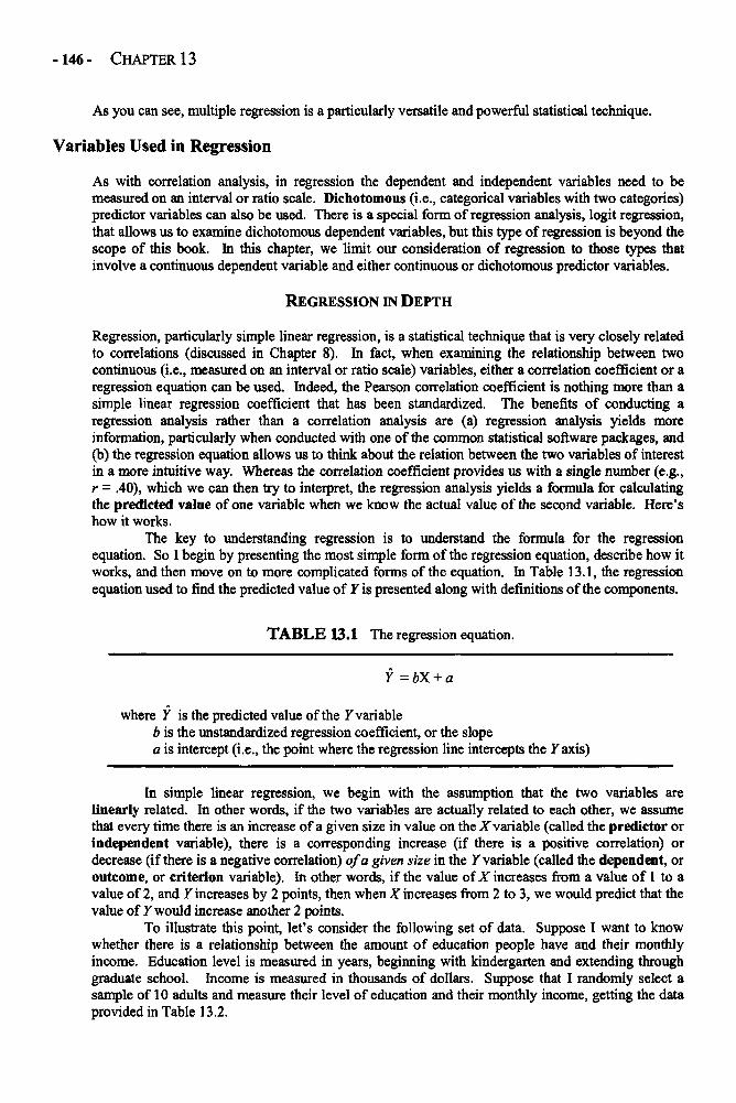
-146- CHAPTER 13
As you can see, multiple regression is a particularly versatile and powerful statistical technique.
Variables Used in Regression
As with correlation analysis, in regression the dependent and independent variables need to bemeasured on an interval or ratio scale. Dichotomous (i.e., categorical variables with two categories)predictor variables can also be used. There is a special form of regression analysis, logit regression,that allows us to examine dichotomous dependent variables, but this type of regression is beyond thescope of this book. In this chapter, we limit our consideration of regression to those types thatinvolve a continuous dependent variable and either continuous or dichotomous predictor variables.
REGRESSION IN DEPTH
Regression, particularly simple linear regression, is a statistical technique that is very closely relatedto correlations (discussed in Chapter 8). In fact, when examining the relationship between twocontinuous (i.e., measured on an interval or ratio scale) variables, either a correlation coefficient or aregression equation can be used. Indeed, the Pearson correlation coefficient is nothing more than asimple linear regression coefficient that has been standardized. The benefits of conducting aregression analysis rather than a correlation analysis are (a) regression analysis yields moreinformation, particularly when conducted with one of the common statistical software packages, and(b) the regression equation allows us to think about the relation between the two variables of interestin a more intuitive way. Whereas the correlation coefficient provides us with a single number (e.g.,r = .40), which we can then try to interpret, the regression analysis yields a formula for calculatingthe predicted value of one variable when we know the actual value of the second variable. Here'show it works.
The key to understanding regression is to understand the formula for the regressionequation. So I begin by presenting the most simple form of the regression equation, describe how itworks, and then move on to more complicated forms of the equation. In Table 13.1, the regressionequation used to find the predicted value of Y is presented along with definitions of the components.
TABLE 13.1 The regression equation.
where Y is the predicted value of the Y variableb is the unstandardized regression coefficient, or the slopea is intercept (i.e., the point where the regression line intercepts the Y axis)
In simple linear regression, we begin with the assumption that the two variables arelinearly related. In other words, if the two variables are actually related to each other, we assumethat every time there is an increase of a given size in value on the X variable (called the predictor orindependent variable), there is a corresponding increase (if there is a positive correlation) ordecrease (if there is a negative correlation) of a given size in the Y variable (called the dependent, oroutcome, or criterion variable). In other words, if the value of X increases from a value of 1 to avalue of 2, and 7 increases by 2 points, then when X increases from 2 to 3, we would predict that thevalue of Y would increase another 2 points.
To illustrate this point, let's consider the following set of data. Suppose I want to knowwhether there is a relationship between the amount of education people have and their monthlyincome. Education level is measured in years, beginning with kindergarten and extending throughgraduate school. Income is measured in thousands of dollars. Suppose that I randomly select asample of 10 adults and measure their level of education and their monthly income, getting the dataprovided in Table 13.2.
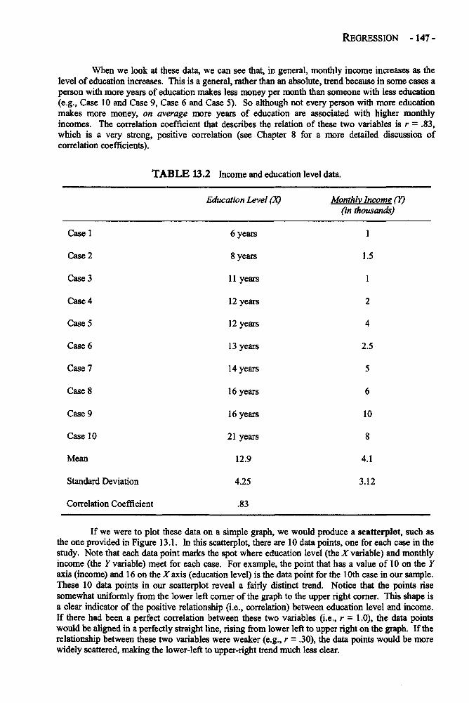
REGRESSION -147 -
When we look at these data, we can see that, in general, monthly income increases as thelevel of education increases. This is a general, rather than an absolute, trend because in some cases aperson with more years of education makes less money per month than someone with less education(e.g., Case 10 and Case 9, Case 6 and Case 5). So although not every person with more educationmakes more money, on average more years of education are associated with higher monthlyincomes. The correlation coefficient that describes the relation of these two variables is r = .83,which is a very strong, positive correlation (see Chapter 8 for a more detailed discussion ofcorrelation coefficients).
TABLE 13.2 Income and education level data.
Education Level (X) Monthly Income (Y)(in thousands)
Case 1
Case 2
Case 3
Case 4
Case 5
Case 6
Case 7
Case 8
Case 9
Case 10
Mean
Standard Deviation
Correlation Coefficient
6 years
8 years
11 years
12 years
12 years
13 years
14 years
16 years
16 years
21 years
12.9
4.25
.83
1
1.5
1
2
4
2.5
5
6
10
8
4.1
3.12
If we were to plot these data on a simple graph, we would produce a scatterpiot, such asthe one provided in Figure 13.1. In this scatterpiot, there are 10 data points, one for each case in thestudy. Note that each data point marks the spot where education level (the X variable) and monthlyincome (the Y variable) meet for each case. For example, the point that has a value of 10 on the Yaxis (income) and 16 on the X axis (education level) is the data point for the 10th case in our sample.These 10 data points in our scatterpiot reveal a fairly distinct trend. Notice that the points risesomewhat uniformly from the lower left corner of the graph to the upper right corner. This shape isa clear indicator of the positive relationship (i.e., correlation) between education level and income.If there had been a perfect correlation between these two variables (i.e., r = 1.0), the data pointswould be aligned in a perfectly straight line, rising from lower left to upper right on the graph. If therelationship between these two variables were weaker (e.g., r = .30), the data points would be morewidely scattered, making the lower-left to upper-right trend much less clear.
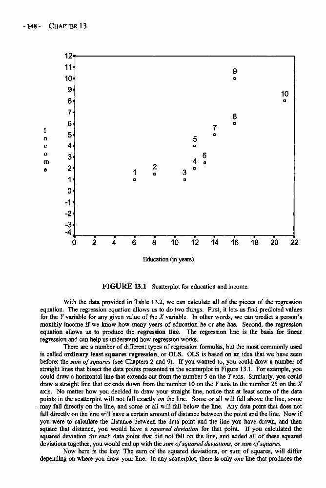
-148- CHAPTER 13
FIGURE 13.1 Scatterplot for education and income.
With the data provided in Table 13.2, we can calculate all of the pieces of the regressionequation. The regression equation allows us to do two things. First, it lets us find predicted valuesfor the Y variable for any given value of the X variable. In other words, we can predict a person'smonthly income if we know how many years of education he or she has. Second, the regressionequation allows us to produce the regression line. The regression line is the basis for linearregression and can help us understand how regression works.
There are a number of different types of regression formulas, but the most commonly usedis called ordinary least squares regression, or OLS. OLS is based on an idea that we have seenbefore: the sum of squares (see Chapters 2 and 9). If you wanted to, you could draw a number ofstraight lines that bisect the data points presented in the scatterplot in Figure 13.1. For example, youcould draw a horizontal line that extends out from the number 5 on the Y axis. Similarly, you coulddraw a straight line that extends down from the number 10 on the 7 axis to the number 25 on the Xaxis. No matter how you decided to draw your straight line, notice that at least some of the datapoints in the scatterplot will not fall exactly on the line. Some or all will fall above the line, somemay fall directly on the line, and some or all will fall below the line. Any data point that does notfall directly on the line will have a certain amount of distance between the point and the line. Now ifyou were to calculate the distance between the data point and the line you have drawn, and thensquare that distance, you would have a squared deviation for that point. If you calculated thesquared deviation for each data point that did not fall on the line, and added all of these squareddeviations together, you would end up with the sum of squared deviations, or sum of squares.
Now here is the key: The sum of the squared deviations, or sum of squares, will differdepending on where you draw your line. In any scatterplot, there is only one line that produces the
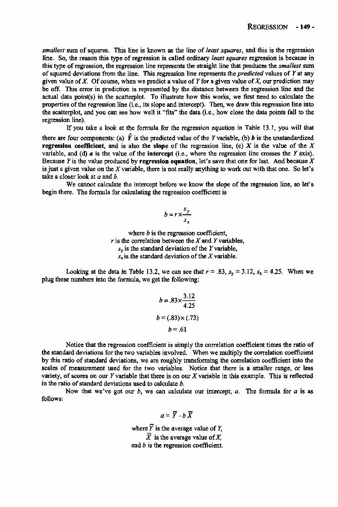
REGRESSION -149 -
smallest sum of squares. This line is known as the line of least squares, and this is the regressionline. So, the reason this type of regression is called ordinary least squares regression is because inthis type of regression, the regression line represents the straight line that produces the smallest sumof squared deviations from the line. This regression line represents the predicted values of Y at anygiven value of X. Of course, when we predict a value of 7 for a given value of X, our prediction maybe off. This error in prediction is represented by the distance between the regression line and theactual data point(s) in the scatterplot. To illustrate how this works, we first need to calculate theproperties of the regression line (i.e., its slope and intercept). Then, we draw this regression line intothe scatterplot, and you can see how well it "fits" the data (i.e., how close the data points fall to theregression line).
If you take a look at the formula for the regression equation in Table 13.1, you will thatthere are four components: (a) Y is the predicted value of the 7 variable, (b) b is the unstandardizedregression coefficient, and is also the slope of the regression line, (c) X is the value of the Xvariable, and (d) a is the value of the intercept (i.e., where the regression line crosses the 7 axis).Because Y is the value produced by regression equation, let's save that one for last. And because Xis just a given value on the X variable, there is not really anything to work out with that one. So let'stake a closer look at a and b.
We cannot calculate the intercept before we know the slope of the regression line, so let'sbegin there. The formula for calculating the regression coefficient is
where b is the regression coefficient,r is the correlation between the X and 7 variables,
sy is the standard deviation of the 7 variable,sx is the standard deviation of the X variable.
Looking at the data in Table 13.2, we can see that r - .83, sy = 3.12, Sx = 4.25. When weplug these numbers into the formula, we get the following:
Notice that the regression coefficient is simply the correlation coefficient times the ratio ofthe standard deviations for the two variables involved. When we multiply the correlation coefficientby this ratio of standard deviations, we are roughly transforming the correlation coefficient into thescales of measurement used for the two variables. Notice that there is a smaller range, or lessvariety, of scores on our 7 variable that there is on our X variable in this example. This is reflectedin the ratio of standard deviations used to calculate b.
Now that we've got our b, we can calculate our intercept, a. The formula for a is asfollows:
a = Y - b X
where 7 is the average value of 7,X is the average value of X,
and b is the regression coefficient.
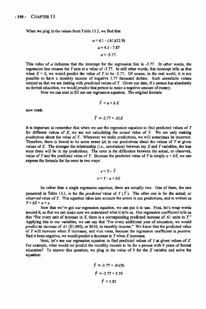
-150- CHAPTER 13
When we plug in the values from Table 13.2, we find that
a = 4.1-(.61)(12.9)
0 = 4.1-7.87
a = -3.77.
This value of a indicates that the intercept for the regression line is -3.77. In other words, theregression line crosses the Y axis at a value of -3.77. In still other words, this intercept tells us thatwhen X = 0, we would predict the value of Y to be -3.77. Of course, in the real world, it is notpossible to have a monthly income of negative 3.77 thousand dollars. Such unrealistic valuesremind us that we are dealing with predicted values of Y. Given our data, if a person has absolutelyno formal education, we would predict that person to make a negative amount of money.
Now we can start to fill out our regression equation. The original formula
now reads
It is important to remember that when we use the regression equation to find predicted values of Yfor different values of X, we are not calculating the actual value of Y. We are only makingpredictions about the value of 7. Whenever we make predictions, we will sometimes be incorrect.Therefore, there is bound to be some error (e) in our predictions about the values of Y at givenvalues of X. The stronger the relationship (i.e., correlation) between my X and 7 variables, the lesserror there will be in my predictions. The error is the difference between the actual, or observed,value of Y and the predicted value of Y. Because the predicted value of Y is simply a + bX, we canexpress the formula for the error in two ways:
So rather than a single regression equation, there are actually two. One of them, the onepresented in Table 13.1, is for the predicted value of Y ( Y ) . The other one is for the actual, orobserved value of 7. This equation takes into account the errors in our predictions, and is written as7= bX+ a + e.
Now that we've got our regression equation, we can put it to use. First, let's wrap wordsaround it, so that we can make sure we understand what it tells us. Our regression coefficient tells usthat "For every unit of increase in X, there is a corresponding predicted increase of .61 units in 7."Applying this to our variables, we can say that "For every additional year of education, we wouldpredict an increase of .61 ($1,000), or $610, in monthly income." We know that the predicted valueof 7 will increase when X increases, and vice versa, because the regression coefficient is positive.Had it been negative, we would predict a decrease in 7 when X increases.
Next, let's use our regression equation to find predicted values of Y at given values of X.For example, what would we predict the monthly income to be for a person with 9 years of formaleducation? To answer this question, we plug in the value of 9 for the X variable and solve theequation:
Y = -3.77 + .61(9)
7 =-3.77 + 5.59
7 =1.82
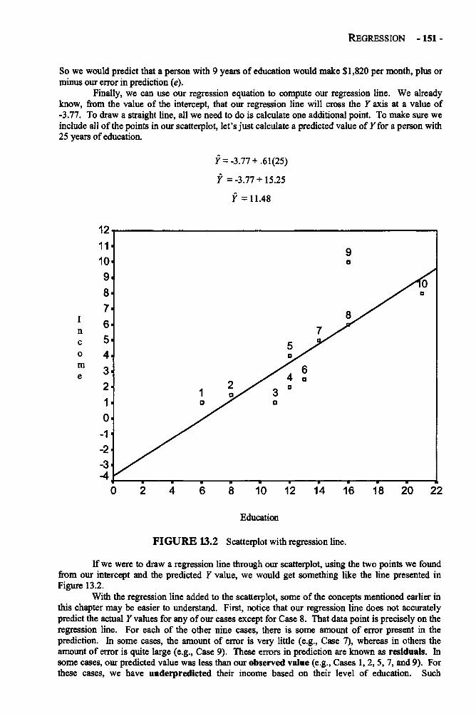
REGRESSION -151 -
So we would predict that a person with 9 years of education would make $1,820 per month, plus orminus our error in prediction (e).
Finally, we can use our regression equation to compute our regression line. We alreadyknow, from the value of the intercept, that our regression line will cross the Y axis at a value of-3.77. To draw a straight line, all we need to do is calculate one additional point. To make sure weinclude all of the points in our scatterplot, let's just calculate a predicted value of Y for a person with25 years of education.
Y = -3.77 + .61(25)
Y = -3.77 + 15.25
Y =11.48
FIGURE 13.2 Scatterplot with regression line.
If we were to draw a regression line through our scatterplot, using the two points we foundfrom our intercept and the predicted 7 value, we would get something like the line presented inFigure 13.2.
With the regression line added to the scatterplot, some of the concepts mentioned earlier inthis chapter may be easier to understand. First, notice that our regression line does not accuratelypredict the actual 7 values for any of our cases except for Case 8. That data point is precisely on theregression line. For each of the other nine cases, there is some amount of error present in theprediction. In some cases, the amount of error is very little (e.g., Case 7), whereas in others theamount of error is quite large (e.g., Case 9). These errors in prediction are known as residuals. Insome cases, our predicted value was less than our observed value (e.g., Cases 1, 2, 5, 7, and 9). Forthese cases, we have underpredicted their income based on their level of education. Such

-152- CHAPTER 13
underpredictions produce positive residuals (because the residual = observed scores - predictedscore). For other cases (Cases 3, 4, 6, and 10) we overpredicted the 7 value, creating negativeresiduals. Second, notice the distance between each case and the line. When we square each ofthese distances and then add them all together, we get the sum of squares. Third, notice that theregression line marks the line where the sum of the squared distances is smallest. To test this, trydrawing some other lines and noting the way it increases the overall amount of error in prediction.Finally, notice where the regression line crosses the Y axis (the intercept) and the how much higherup the Y axis the regression line goes for each increase of one unit value in X (the slope). The slopeand the intercept will correspond with the values that we found for b and a, respectively.
MULTIPLE REGRESSION
Now that we've discussed the elements of simple linear regression, let's move on to a considerationof multiple regression. Despite the impressive qualities of simple linear regression, the plain truthis that when we only have two variables, simple linear regression does not provide much moreinformation than would a simple correlation coefficient. Because of this, you rarely see a simplelinear regression with two variables reported in a published study. But multiple regression is awhole different story. Multiple regression is a very powerful statistic that can be used to provide astaggering array of useful information. At this point, it may be worth reminding you that in a shortbook like this, we only scratch the surface of what multiple regression can do and how it works. Theinterested reader should refer to one or all of the references listed at the end of this chapter to findmore information on this powerful technique.
To illustrate some of the benefits of multiple regression, let's add a second predictorvariable to our example. So far, using the data from Table 13.2, we have examined the relationshipbetween education level and income. In this example, education level has been used as our predictoror independent variable and income has been used as our dependent or outcome variable. We foundthat, on average, in our sample one's monthly salary is predicted to increase by $610 for everyadditional year of schooling the individual has received. But there was some error in ourpredictions, indicating that there are other variables that predict how much money one makes. Onesuch predictor may be the length of time one has been out of school. Because people tend to makemore money the longer they have been in the workforce, it stands to reason that those adults in oursample who finished school a long time ago may be making more than those who finished schoolmore recently. Although Case 4 and Case 5 each had 12 years of schooling, Case 5 makes moremoney than Case 4. Perhaps this is due to Case 5 being in the workforce longer than Case 4.
When we add this second predictor variable to the model, we get the following regressionequation:
where Y is the predicted value of the dependent variable,X1 is the value of the first predictor variable,
and X2 is the value of the second predictor variable.
This regression equation with two predictor variables will allow me to examine a number ofdifferent questions. First, I can see whether my two predictor variables, combined, are significantlyrelated to, or predictive of, my dependent variable, and how much of the variance my predictorvariables explain in my dependent variable. Second, I can test whether each of my predictorvariables is significantly related to my dependent variable when controlling for the other predictorvariable. When I say "controlling for the other predictor variable," I mean that I can examinewhether a predictor variable is related to the dependent variable after I partial out, or take away, theportion of the variance in my dependent variable that has already been accounted for by my otherindependent variable. Third, I can see which of my two predictor variables is the stronger predictorof my dependent variable. Fourth, I can test whether one predictor variable is related to mydependent variable after controlling for the other predictor variable, thus conducting a sort of
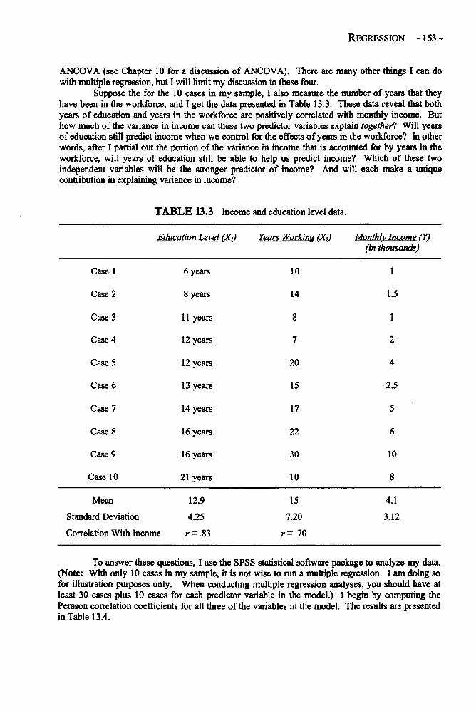
REGRESSION -153 -
ANCOVA (see Chapter 10 for a discussion of ANCOVA). There are many other things I can dowith multiple regression, but I will limit my discussion to these four.
Suppose the for the 10 cases in my sample, I also measure the number of years that theyhave been in the workforce, and I get the data presented in Table 13.3. These data reveal that bothyears of education and years in the workforce are positively correlated with monthly income. Buthow much of the variance in income can these two predictor variables explain together? Will yearsof education still predict income when we control for the effects of years in the workforce? In otherwords, after I partial out the portion of the variance in income that is accounted for by years in theworkforce, will years of education still be able to help us predict income? Which of these twoindependent variables will be the stronger predictor of income? And will each make a uniquecontribution in explaining variance in income?
TABLE 13.3 Income and education level data.
Education Level (X1) Years Working (X2) Monthly Income (Y)(in thousands)
Case 1
Case 2
Case 3
Case 4
Case 5
Case 6
Case 7
Case 8
Case 9
Case 10
Mean
Standard Deviation
Correlation With Income
6 years
8 years
11 years
12 years
12 years
13 years
14 years
16 years
16 years
21 years
12.9
4.25
r = .83
10
14
8
7
20
15
17
22
30
10
15
7.20
r =.70
1
1.5
1
2
4
2.5
5
6
10
8
4.1
3.12
To answer these questions, I use the SPSS statistical software package to analyze my data.(Note: With only 10 cases in my sample, it is not wise to run a multiple regression. I am doing sofor illustration purposes only. When conducting multiple regression analyses, you should have atleast 30 cases plus 10 cases for each predictor variable in the model.) I begin by computing thePerason correlation coefficients for all three of the variables in the model. The results are presentedin Table 13.4.
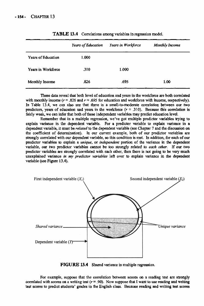
-154- CHAPTER 13
TABLE 13.4 Correlations among variables in regression model.
Years of Education Years in Workforce Monthly Income
Years of Education 1.000
Years in Workforce
Monthly Income
.310
.826
1.000
.695 1.00
These data reveal that both level of education and years in the workforce are both correlatedwith monthly income (r = .826 and r = .695 for education and workforce with income, respectively).In Table 13.4, we can also see that there is a small-to-moderate correlation between our twopredictors, years of education and years in the workforce (r = .310). Because this correlation isfairly weak, we can infer that both of these independent variables may predict education level.
Remember that in a multiple regression, we've got multiple predictor variables trying toexplain variance in the dependent variable. For a predictor variable to explain variance in adependent variable, it must be related to the dependent variable (see Chapter 7 and the discussion onthe coefficient of determination). In our current example, both of our predictor variables arestrongly correlated with our dependent variable, so this condition is met. In addition, for each of ourpredictor variables to explain a unique, or independent portion of the variance in the dependentvariable, our two predictor variables cannot be too strongly related to each other. If our twopredictor variables are strongly correlated with each other, then there is not going to be very muchunexplained variance in my predictor variables left over to explain variance in the dependentvariable (see Figure 13.4).
FIGURE 13.4 Shared variance in multiple regression.
For example, suppose that the correlation between scores on a reading test are stronglycorrelated with scores on a writing test (r = .90). Now suppose that I want to use reading and writingtest scores to predict students' grades in the English class. Because reading and writing test scores
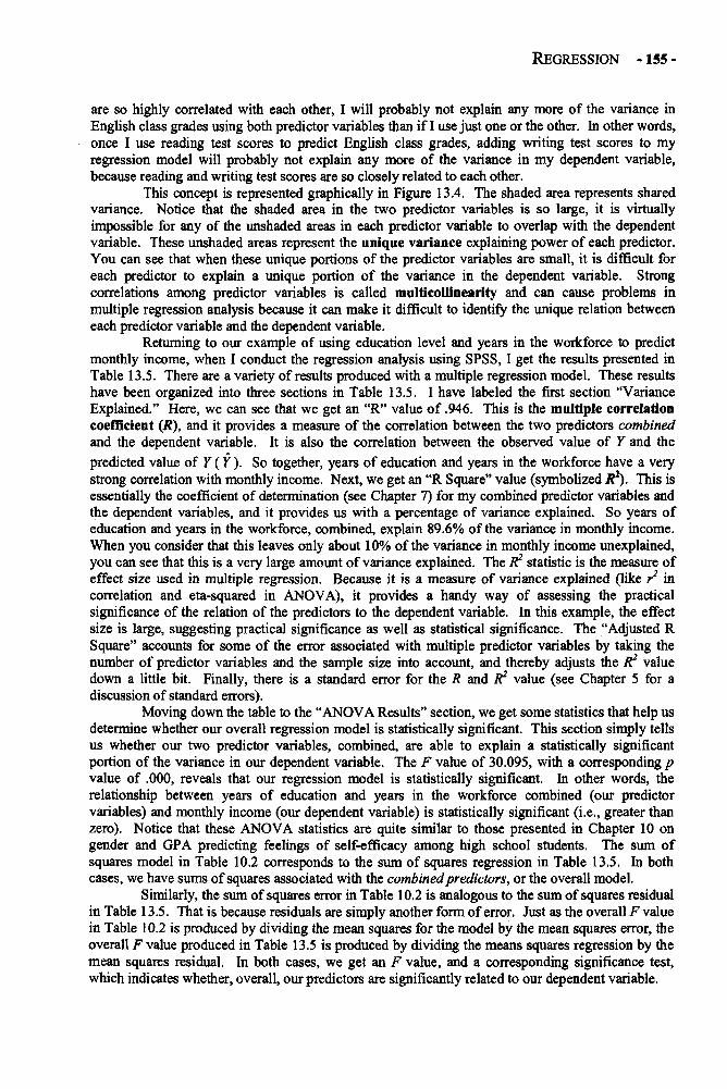
REGRESSION -155 -
are so highly correlated with each other, I will probably not explain any more of the variance inEnglish class grades using both predictor variables than if I use just one or the other. In other words,once I use reading test scores to predict English class grades, adding writing test scores to myregression model will probably not explain any more of the variance in my dependent variable,because reading and writing test scores are so closely related to each other.
This concept is represented graphically in Figure 13.4. The shaded area represents sharedvariance. Notice that the shaded area in the two predictor variables is so large, it is virtuallyimpossible for any of the unshaded areas in each predictor variable to overlap with the dependentvariable. These unshaded areas represent the unique variance explaining power of each predictor.You can see that when these unique portions of the predictor variables are small, it is difficult foreach predictor to explain a unique portion of the variance in the dependent variable. Strongcorrelations among predictor variables is called multicollinearity and can cause problems inmultiple regression analysis because it can make it difficult to identify the unique relation betweeneach predictor variable and the dependent variable.
Returning to our example of using education level and years in the workforce to predictmonthly income, when I conduct the regression analysis using SPSS, I get the results presented inTable 13.5. There are a variety of results produced with a multiple regression model. These resultshave been organized into three sections in Table 13.5. I have labeled the first section "VarianceExplained." Here, we can see that we get an "R" value of .946. This is the multiple correlationcoefficient (R), and it provides a measure of the correlation between the two predictors combinedand the dependent variable. It is also the correlation between the observed value of Y and the
predicted value of Y (Y ). So together, years of education and years in the workforce have a verystrong correlation with monthly income. Next, we get an "R Square" value (symbolized R2). This isessentially the coefficient of determination (see Chapter 7) for my combined predictor variables andthe dependent variables, and it provides us with a percentage of variance explained. So years ofeducation and years in the workforce, combined, explain 89.6% of the variance in monthly income.When you consider that this leaves only about 10% of the variance in monthly income unexplained,you can see that this is a very large amount of variance explained. The R2 statistic is the measure ofeffect size used in multiple regression. Because it is a measure of variance explained (like r2 incorrelation and eta-squared in ANOVA), it provides a handy way of assessing the practicalsignificance of the relation of the predictors to the dependent variable. In this example, the effectsize is large, suggesting practical significance as well as statistical significance. The "Adjusted RSquare" accounts for some of the error associated with multiple predictor variables by taking thenumber of predictor variables and the sample size into account, and thereby adjusts the R2 valuedown a little bit. Finally, there is a standard error for the R and R2 value (see Chapter 5 for adiscussion of standard errors).
Moving down the table to the "ANOVA Results" section, we get some statistics that help usdetermine whether our overall regression model is statistically significant. This section simply tellsus whether our two predictor variables, combined, are able to explain a statistically significantportion of the variance in our dependent variable. The F value of 30.095, with a corresponding pvalue of .000, reveals that our regression model is statistically significant. In other words, therelationship between years of education and years in the workforce combined (our predictorvariables) and monthly income (our dependent variable) is statistically significant (i.e., greater thanzero). Notice that these ANOVA statistics are quite similar to those presented in Chapter 10 ongender and GPA predicting feelings of self-efficacy among high school students. The sum ofsquares model in Table 10.2 corresponds to the sum of squares regression in Table 13.5. In bothcases, we have sums of squares associated with the combined predictors, or the overall model.
Similarly, the sum of squares error in Table 10.2 is analogous to the sum of squares residualin Table 13.5. That is because residuals are simply another form of error. Just as the overall F valuein Table 10.2 is produced by dividing the mean squares for the model by the mean squares error, theoverall F value produced in Table 13.5 is produced by dividing the means squares regression by themean squares residual. In both cases, we get an F value, and a corresponding significance test,which indicates whether, overall, our predictors are significantly related to our dependent variable.
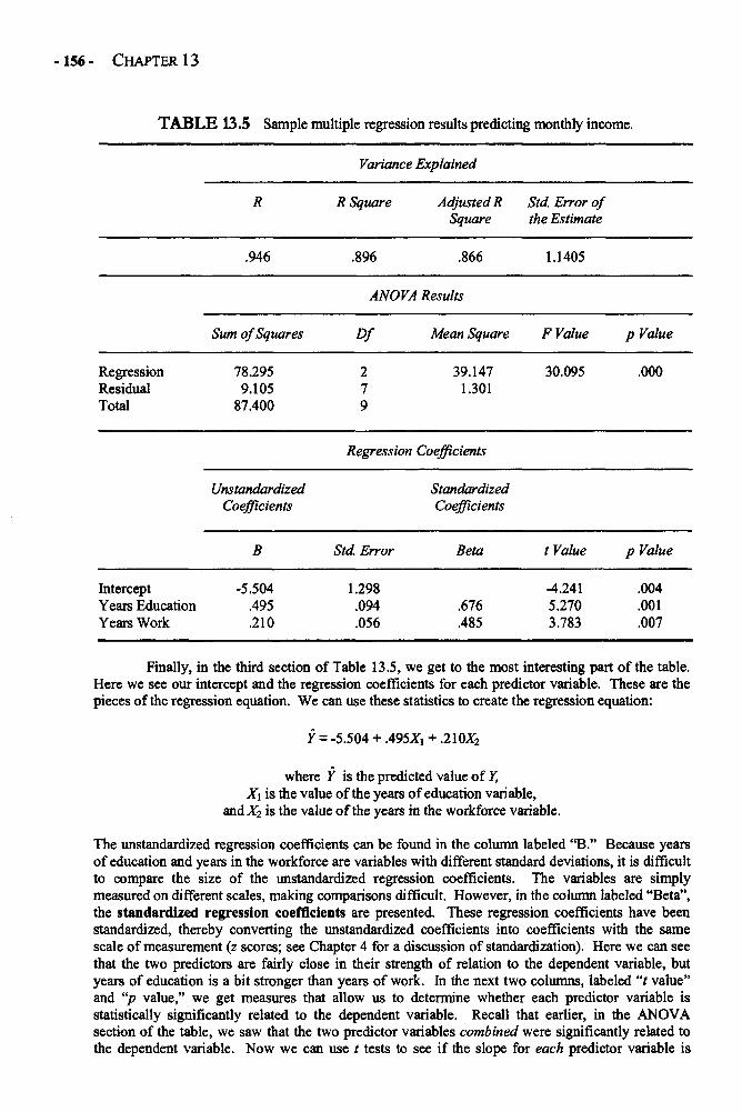
-156- CHAPTER 13
TABLE 13.5 Sample multiple regression results predicting monthly income.
R
Variance Explained
R Square Adjusted R Std, Error ofSquare the Estimate
.946 .896 .866 1.1405
ANOVA Results
RegressionResidualTotal
Sum of Squares
78.2959.105
87.400
Df
219
Mean Square F Value
39.147 30.0951.301
p Value
.000
Regression Coefficients
UnstandardizedCoefficients
StandardizedCoefficients
B Std. Error Beta t Value p Value
InterceptYears EducationYears Work
-5.504.495.210
1.298.094.056
.676
.485
-4.2415.2703.783
.004
.001
.007
Finally, in the third section of Table 13.5, we get to the most interesting part of the table.Here we see our intercept and the regression coefficients for each predictor variable. These are thepieces of the regression equation. We can use these statistics to create the regression equation:
where Y is the predicted value of Y,X1 is the value of the years of education variable,
and X2 is the value of the years in the workforce variable.
The unstandardized regression coefficients can be found in the column labeled "B." Because yearsof education and years in the workforce are variables with different standard deviations, it is difficultto compare the size of the unstandardized regression coefficients. The variables are simplymeasured on different scales, making comparisons difficult. However, in the column labeled "Beta",the standardized regression coefficients are presented. These regression coefficients have beenstandardized, thereby converting the unstandardized coefficients into coefficients with the samescale of measurement (z scores; see Chapter 4 for a discussion of standardization). Here we can seethat the two predictors are fairly close in their strength of relation to the dependent variable, butyears of education is a bit stronger than years of work. In the next two columns, labeled "t value"and "p value," we get measures that allow us to determine whether each predictor variable isstatistically significantly related to the dependent variable. Recall that earlier, in the ANOVAsection of the table, we saw that the two predictor variables combined were significantly related tothe dependent variable. Now we can use t tests to see if the slope for each predictor variable is
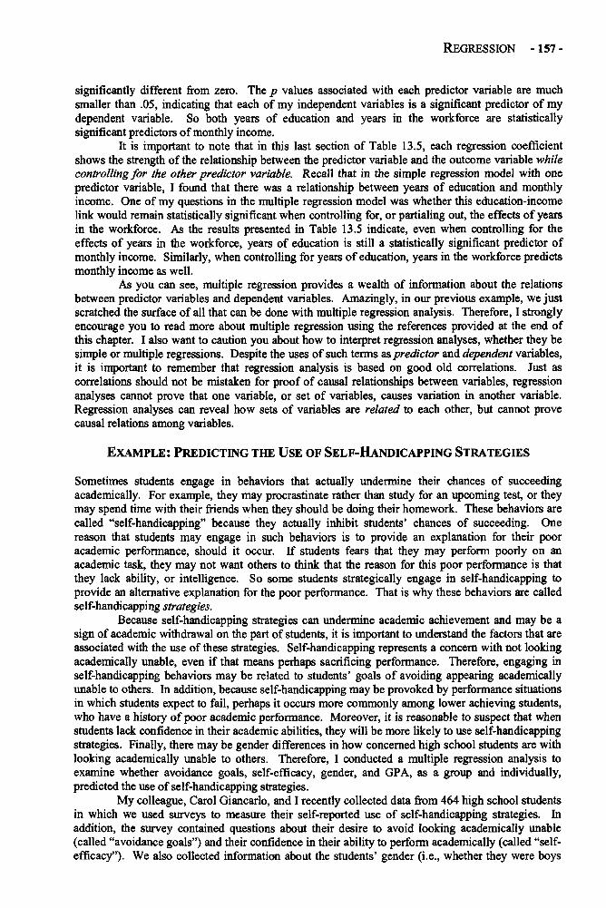
REGRESSION - 157 -
significantly different from zero. The p values associated with each predictor variable are muchsmaller than .05, indicating that each of my independent variables is a significant predictor of mydependent variable. So both years of education and years in the workforce are statisticallysignificant predictors of monthly income.
It is important to note that in this last section of Table 13.5, each regression coefficientshows the strength of the relationship between the predictor variable and the outcome variable whilecontrolling for the other predictor variable. Recall that in the simple regression model with onepredictor variable, I found that there was a relationship between years of education and monthlyincome. One of my questions in the multiple regression model was whether this education-incomelink would remain statistically significant when controlling for, or partialing out, the effects of yearsin the workforce. As the results presented in Table 13.5 indicate, even when controlling for theeffects of years in the workforce, years of education is still a statistically significant predictor ofmonthly income. Similarly, when controlling for years of education, years in the workforce predictsmonthly income as well.
As you can see, multiple regression provides a wealth of information about the relationsbetween predictor variables and dependent variables. Amazingly, in our previous example, we justscratched the surface of all that can be done with multiple regression analysis. Therefore, I stronglyencourage you to read more about multiple regression using the references provided at the end ofthis chapter. I also want to caution you about how to interpret regression analyses, whether they besimple or multiple regressions. Despite the uses of such terms as predictor and dependent variables,it is important to remember that regression analysis is based on good old correlations. Just ascorrelations should not be mistaken for proof of causal relationships between variables, regressionanalyses cannot prove that one variable, or set of variables, causes variation in another variable.Regression analyses can reveal how sets of variables are related to each other, but cannot provecausal relations among variables.
EXAMPLE: PREDICTING THE USE OF SELF-HANDICAPPING STRATEGIES
Sometimes students engage in behaviors that actually undermine their chances of succeedingacademically. For example, they may procrastinate rather than study for an upcoming test, or theymay spend time with their friends when they should be doing their homework. These behaviors arecalled "self-handicapping" because they actually inhibit students' chances of succeeding. Onereason that students may engage in such behaviors is to provide an explanation for their pooracademic performance, should it occur. If students fears that they may perform poorly on anacademic task, they may not want others to think that the reason for this poor performance is thatthey lack ability, or intelligence. So some students strategically engage in self-handicapping toprovide an alternative explanation for the poor performance. That is why these behaviors are calledself-handicapping strategies.
Because self-handicapping strategies can undermine academic achievement and may be asign of academic withdrawal on the part of students, it is important to understand the factors that areassociated with the use of these strategies. Self-handicapping represents a concern with not lookingacademically unable, even if that means perhaps sacrificing performance. Therefore, engaging inself-handicapping behaviors may be related to students' goals of avoiding appearing academicallyunable to others. In addition, because self-handicapping may be provoked by performance situationsin which students expect to fail, perhaps it occurs more commonly among lower achieving students,who have a history of poor academic performance. Moreover, it is reasonable to suspect that whenstudents lack confidence in their academic abilities, they will be more likely to use self-handicappingstrategies. Finally, there may be gender differences in how concerned high school students are withlooking academically unable to others. Therefore, I conducted a multiple regression analysis toexamine whether avoidance goals, self-efficacy, gender, and GPA, as a group and individually,predicted the use of self-handicapping strategies.
My colleague, Carol Giancarlo, and I recently collected data from 464 high school studentsin which we used surveys to measure their self-reported use of self-handicapping strategies. Inaddition, the survey contained questions about their desire to avoid looking academically unable(called "avoidance goals") and their confidence in their ability to perform academically (called "self-efficacy"). We also collected information about the students' gender (i.e., whether they were boys
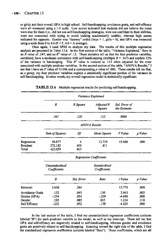
-158- CHAPTER 13
or girls) and their overall GPA in high school. Self-handicapping, avoidance goals, and self-efficacywere all measured using a 1-5 scale. Low scores indicated that students did not believe the itemswere true for them (i.e., did not use self-handicapping strategies, were not confident in their abilities,were not concerned with trying to avoid looking academically unable), whereas high scoresindicated the opposite. Gender was "dummy" coded (boys = 1, girls = 0), and GPA was measuredusing a scale from 0 to 4.0 (0 = F, 4.0 = A average).
Once again, I used SPSS to analyze my data. The results of this multiple regressionanalysis are presented in Table 13.6. In the first section of the table, "Variance Explained," there isan R value of .347, and an R2 value of .12. These statistics tell us that the four predictor variables,combined, have a moderate correlation with self-handicapping (multiple R = .347) and explain 12%of the variance in handicaping. This R2 value is reduced to .113 when adjusted for the errorassociated with multiple predictor variables. In the second section of the table, "ANOVA Results," Isee that I have an F value of 15.686 and a corresponding p value of .000. These results tell me that,as a group, my four predictor variables explain a statistically significant portion of the variance inself-handicapping. In other words, my overall regression model is statistically significant.
TABLE 13.6 Multiple regression results for predicting self-handicapping.
R
Variance Explained
R Square Adjusted R Std. Error ofSquare the Estimate
.347 .120 .113 .9005
ANOVA Results
Sum of Squares Df Mean Square F Value p Value
RegressionResidualTotal
50.877372.182423.059
4459463
12.719 15.686.811
.000
Regression Coefficients
UnstandardizedCoefficients
Intercept
Avoidance GoalsGrades (GPA)GenderSelf Efficacy
B
3.630
.132-.254.105
-.232
Std. Error
.264
.045
.054
.085
.052
StandardizedCoefficients
Beta
.130-.209.055-.198
t Value
13.775
2.943-4.6901.234
-4.425
p Value
.000
.003
.000
.218
.000
In the last section of the table, I find my unstandardized regression coefficients (columnlabeled "B") for each predictor variable in the model, as well as my intercept. These tell me thatGPA and self-efficacy are negatively related to self-handicapping, whereas gender and avoidancegoals are positively related to self-handicapping. Scanning toward the right side of the table, I findthe standardized regression coefficients (column labeled "Beta"). These coefficients, which are all
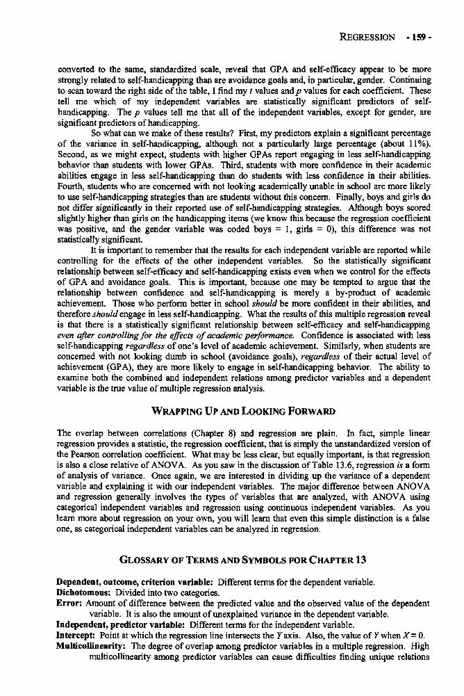
REGRESSION -159 -
converted to the same, standardized scale, reveal that GPA and self-efficacy appear to be morestrongly related to self-handicapping than are avoidance goals and, in particular, gender. Continuingto scan toward the right side of the table, I find my t values and p values for each coefficient. Thesetell me which of my independent variables are statistically significant predictors of self-handicapping. The p values tell me that all of the independent variables, except for gender, aresignificant predictors of handicapping.
So what can we make of these results? First, my predictors explain a significant percentageof the variance in self-handicapping, although not a particularly large percentage (about 11%).Second, as we might expect, students with higher GPAs report engaging in less self-handicappingbehavior than students with lower GPAs. Third, students with more confidence in their academicabilities engage in less self-handicapping than do students with less confidence in their abilities.Fourth, students who are concerned with not looking academically unable in school are more likelyto use self-handicapping strategies than are students without this concern. Finally, boys and girls donot differ significantly in their reported use of self-handicapping strategies. Although boys scoredslightly higher than girls on the handicapping items (we know this because the regression coefficientwas positive, and the gender variable was coded boys = 1, girls = 0), this difference was notstatistically significant.
It is important to remember that the results for each independent variable are reported whilecontrolling for the effects of the other independent variables. So the statistically significantrelationship between self-efficacy and self-handicapping exists even when we control for the effectsof GPA and avoidance goals. This is important, because one may be tempted to argue that therelationship between confidence and self-handicapping is merely a by-product of academicachievement. Those who perform better in school should be more confident in their abilities, andtherefore should engage in less self-handicapping. What the results of this multiple regression revealis that there is a statistically significant relationship between self-efficacy and self-handicappingeven after controlling for the effects of academic performance. Confidence is associated with lessself-handicapping regardless of one's level of academic achievement. Similarly, when students areconcerned with not looking dumb in school (avoidance goals), regardless of their actual level ofachievement (GPA), they are more likely to engage in self-handicapping behavior. The ability toexamine both the combined and independent relations among predictor variables and a dependentvariable is the true value of multiple regression analysis.
WRAPPING UP AND LOOKING FORWARD
The overlap between correlations (Chapter 8) and regression are plain. In fact, simple linearregression provides a statistic, the regression coefficient, that is simply the unstandardized version ofthe Pearson correlation coefficient. What may be less clear, but equally important, is that regressionis also a close relative of ANOVA. As you saw in the discussion of Table 13.6, regression is a formof analysis of variance. Once again, we are interested in dividing up the variance of a dependentvariable and explaining it with our independent variables. The major difference between ANOVAand regression generally involves the types of variables that are analyzed, with ANOVA usingcategorical independent variables and regression using continuous independent variables. As youlearn more about regression on your own, you will learn that even this simple distinction is a falseone, as categorical independent variables can be analyzed in regression.
GLOSSARY OF TERMS AND SYMBOLS FOR CHAPTER 13
Dependent, outcome, criterion variable: Different terms for the dependent variable.Dichotomous: Divided into two categories.Error: Amount of difference between the predicted value and the observed value of the dependent
variable. It is also the amount of unexplained variance in the dependent variable.Independent, predictor variable: Different terms for the independent variable.Intercept: Point at which the regression line intersects the Y axis. Also, the value of 7 when X- 0.Multicollinearity: The degree of overlap among predictor variables in a multiple regression. High
multicollinearity among predictor variables can cause difficulties finding unique relations
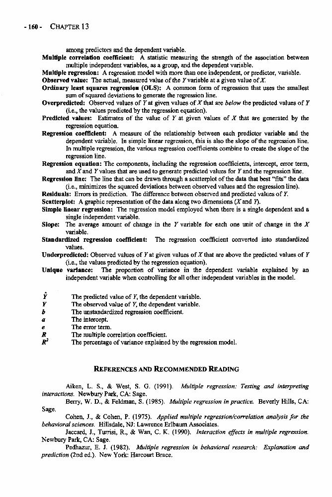
-160- CHAPTER 13
among predictors and the dependent variable.Multiple correlation coefficient: A statistic measuring the strength of the association between
multiple independent variables, as a group, and the dependent variable.Multiple regression: A regression model with more than one independent, or predictor, variable.Observed value: The actual, measured value of the 7 variable at a given value of X.Ordinary least squares regression (OLS): A common form of regression that uses the smallest
sum of squared deviations to generate the regression line.Overpredicted: Observed values of 7 at given values of X that are below the predicted values of 7
(i.e., the values predicted by the regression equation).Predicted values: Estimates of the value of 7 at given values of X that are generated by the
regression equation.Regression coefficient: A measure of the relationship between each predictor variable and the
dependent variable. In simple linear regression, this is also the slope of the regression line.In multiple regression, the various regression coefficients combine to create the slope of theregression line.
Regression equation: The components, including the regression coefficients, intercept, error term,and X and Y values that are used to generate predicted values for Y and the regression line.
Regression line: The line that can be drawn through a scatterplot of the data that best "fits" the data(i.e., minimizes the squared deviations between observed values and the regression line).
Residuals: Errors in prediction. The difference between observed and predicted values of 7.Scatterplot: A graphic representation of the data along two dimensions (X and Y).Simple linear regression: The regression model employed when there is a single dependent and a
single independent variable.Slope: The average amount of change in the 7 variable for each one unit of change in the X
variable.Standardized regression coefficient: The regression coefficient converted into standardized
values.Underpredicted: Observed values of Y at given values of X that are above the predicted values of 7
(i.e., the values predicted by the regression equation).Unique variance: The proportion of variance in the dependent variable explained by an
independent variable when controlling for all other independent variables in the model.
A
Y The predicted value of 7, the dependent variable.Y The observed value of 7, the dependent variable.b The unstandardized regression coefficient.a The intercept.e The error term.R The multiple correlation coefficient.R2 The percentage of variance explained by the regression model.
REFERENCES AND RECOMMENDED READING
Aiken, L. S., & West, S. G. (1991). Multiple regression: Testing and interpretinginteractions. Newbury Park, CA: Sage.
Berry, W. D., & Feldman, S. (1985). Multiple regression in practice. Beverly Hills, CA:Sage.
Cohen, J., & Cohen, P. (1975). Applied multiple regression/correlation analysis for thebehavioral sciences. Hillsdale, NJ: Lawrence Erlbaum Associates.
Jaccard, J., Turrisi, R., & Wan, C. K. (1990). Interaction effects in multiple regression.Newbury Park, CA: Sage.
Pedhazur, E. J. (1982). Multiple regression in behavioral research: Explanation andprediction (2nd ed.). New York: Harcourt Brace.
CHAPTER 14
THE CHI-SQUARE TEST OF INDEPENDENCE
All of the inferential statistics discussed in this book share a set of assumptions. Regression,ANOVA, correlation, and t tests all assume that the data involved are scores on some measure (e.g.,IQ scores, height, income, scores on a measure of depression) calculated from samples drawn frompopulations that are normally distributed, and everything is hunky-dory in the world of research. Ofcourse, as discussed in Chapter 1, these conditions are often not met in social science research.Populations are sometimes skewed rather than normal. Sometimes researchers want to know aboutthings besides those that can be measured. Research is often messy and unpredictable rather thanhunky-dory.
The violation of these assumptions represents sort of a good news, bad news situation. The badnews is that if the assumptions are violated to an alarming degree, the results of these statistics canbe difficult to interpret, even meaningless. The good news is that "to an alarming degree" is animprecise phrase and open to interpretation. In many situations, violating assumptions of normallydistributed data often do not make the results invalid, or even alter them very much. Another pieceof good news is that even when the assumptions of these statistics are horrifically violated, there is awhole batch of statistics that researchers can use that do not have the same assumptions of normalityand random selection: nonparametric statistics.
There are a number of nonparametric tests available. The Mann-Whitney U test is sort of anonparametric equivalent of the independent t test. The Kruskal-Wallis analysis of variance forranked data can be roughly substituted for the one-way ANOVA for continuously scaled variables.These nonparametric statistics can be extremely useful, and descriptions of their uses andcharacteristics can be found in most standard-length statistics textbooks. In this chapter, I limit myattention to one of the most commonly used nonparametric tests: the chi-square (x2) test ofindependence. This test is appropriate for use when you have data from two categorical, ornominally scaled, variables (see Chapter 1 for a description of these variable types). Withcategorical variables, the cases in your sample are divided among the different categories of yourcategorical variables. For example, gender is a categorical variable and the cases in a sample ofhuman beings can be divided into male and female, the two categories of the gender variable. Whenyou have two categorical variables, you may want to know whether the division of cases in onevariable is independent of the other categorical variable. For example, suppose you have a sample ofboys and girls from the 5th, 8th, and 12th grades of school. You may want to know whether yourrepresentation of boys and girls depends on their grade level, or if the division of boys and girls isabout what you would expect independent of grade level. That is the type of question that the chi-square test of independence was designed to answer.
A more precise way of stating the purpose of the chi-square test of independence is this: Itallows you to determine whether cases in a sample fall into categories in proportions equal to whatone would expect by chance. For example, suppose that you work in a liberal arts college. Youwant to know whether the men and women in your college differ in their selection of majors. So yourandomly select 100 men and 100 women and ask them to tell you their major. You get the datapresented in Table 14.1.
Does this distribution of data represent a statistically significant gender difference inmajors? Before you can answer that question, you need to know more information. Specifically,you need to determine how many men and women you expect to major in these three areas just basedon the number of each gender and each major in the sample. This is the type of question that the chi-square test of independence allows you to answer.
-161-
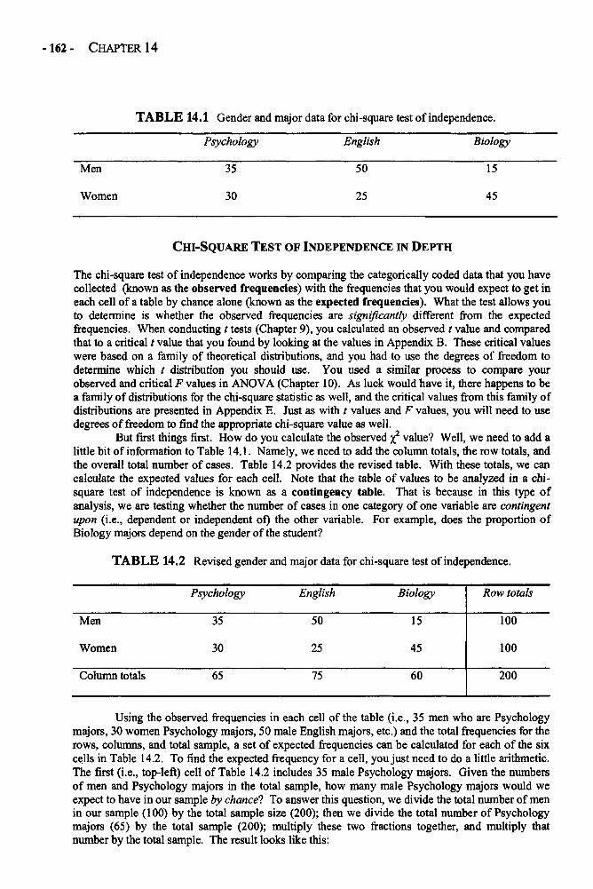
-162- CHAPTER 14
TABLE 14.1 Gender and major data for chi-square test of independence.
Psychology English Biology
Women 30 25 45
CHI-SQUARE TEST OF INDEPENDENCE IN DEPTH
The chi-square test of independence works by comparing the categorically coded data that you havecollected (known as the observed frequencies) with the frequencies that you would expect to get ineach cell of a table by chance alone (known as the expected frequencies). What the test allows youto determine is whether the observed frequencies are significantly different from the expectedfrequencies. When conducting t tests (Chapter 9), you calculated an observed t value and comparedthat to a critical t value that you found by looking at the values in Appendix B. These critical valueswere based on a family of theoretical distributions, and you had to use the degrees of freedom todetermine which t distribution you should use. You used a similar process to compare yourobserved and critical F values in ANOVA (Chapter 10). As luck would have it, there happens to bea family of distributions for the chi-square statistic as well, and the critical values from this family ofdistributions are presented in Appendix E. Just as with t values and F values, you will need to usedegrees of freedom to find the appropriate chi-square value as well.
But first tilings first. How do you calculate the observed x2 value? Well, we need to add alittle bit of information to Table 14.1. Namely, we need to add the column totals, the row totals, andthe overall total number of cases. Table 14.2 provides the revised table. With these totals, we cancalculate the expected values for each cell. Note that the table of values to be analyzed in a chi-square test of independence is known as a contingency table. That is because in this type ofanalysis, we are testing whether the number of cases in one category of one variable are contingentupon (i.e., dependent or independent of) the other variable. For example, does the proportion ofBiology majors depend on the gender of the student?
TABLE 14.2 Revised gender and major data for chi-square test of independence.
Men
Women
Column totals
Psychology
35
30
65
English
50
25
75
Biology
15
45
60
Row totals
100
100
200
Using the observed frequencies in each cell of the table (i.e., 35 men who are Psychologymajors, 30 women Psychology majors, 50 male English majors, etc.) and the total frequencies for therows, columns, and total sample, a set of expected frequencies can be calculated for each of the sixcells in Table 14.2. To find the expected frequency for a cell, you just need to do a little arithmetic.The first (i.e., top-left) cell of Table 14.2 includes 35 male Psychology majors. Given the numbersof men and Psychology majors in the total sample, how many male Psychology majors would weexpect to have in our sample by chance? To answer this question, we divide the total number of menin our sample (100) by the total sample size (200); then we divide the total number of Psychologymajors (65) by the total sample (200); multiply these two fractions together, and multiply thatnumber by the total sample. The result looks like this:
Men 35 50 15
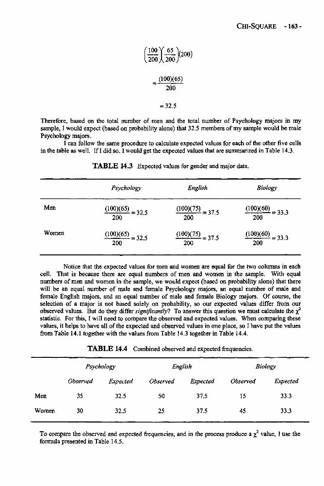
v
Therefore, based on the total number of men and the total number of Psychology majors in mysample, I would expect (based on probability alone) that 32.5 members of my sample would be malePsychology majors.
I can follow the same procedure to calculate expected values for each of the other five cellsin the table as well. If I did so, I would get the expected values that are summarized in Table 14.3.
TABLE 14.3 Expected values for gender and major data.
Psychology English Biology
Men
Women
Notice that the expected values for men and women are equal for the two columns in eachcell. That is because there are equal numbers of men and women in the sample. With equalnumbers of men and women in the sample, we would expect (based on probability alone) that therewill be an equal number of male and female Psychology majors, an equal number of male andfemale English majors, and an equal number of male and female Biology majors. Of course, theselection of a major is not based solely on probability, so our expected values differ from ourobserved values. But do they differ significantly? To answer this question we must calculate the x2
statistic. For this, I will need to compare the observed and expected values. When comparing thesevalues, it helps to have all of the expected and observed values in one place, so I have put the valuesfrom Table 14.1 together with the values from Table 14.3 together in Table 14.4.
TABLE 14.4 Combined observed and expected frequencies.
Psychology English Biology
Observed Expected Observed Expected Observed Expected
Men 35 32.5 50 37.5 15 33.3
Women 30 32.5 25 37.5 45 33.3
To compare the observed and expected frequencies, and in the process produce a x2 value, I use theformula presented in Table 14.5.
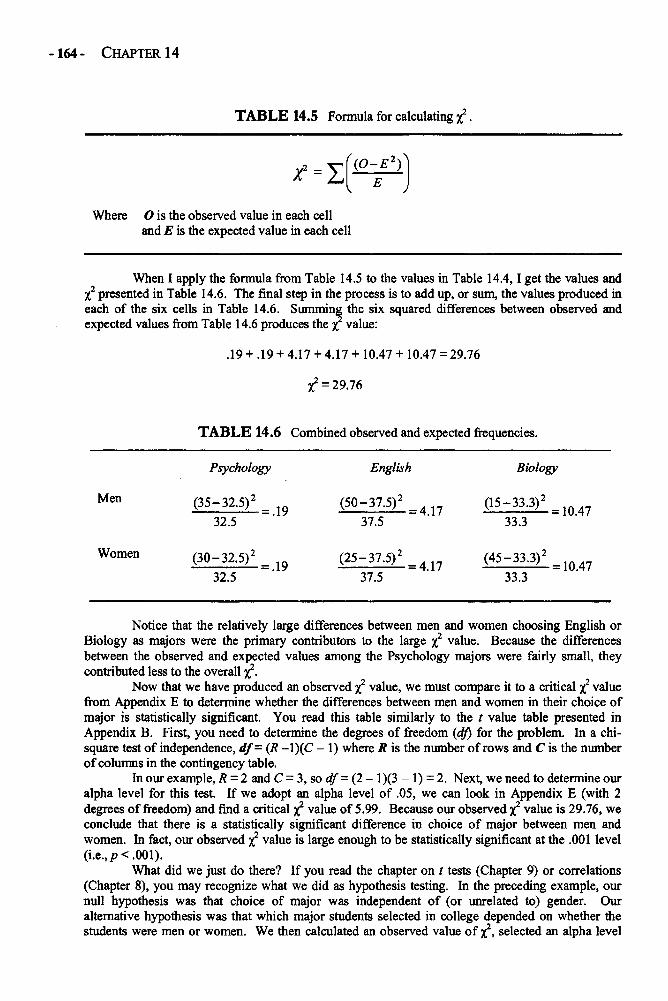
-164- CHAPTER 14
TABLE 14.5 Formula for calculating x2
Where O is the observed value in each celland E is the expected value in each cell
When I apply the formula from Table 14.5 to the values in Table 14.4, I get the values andX2 presented in Table 14.6. The final step in the process is to add up, or sum, the values produced ineach of the six cells in Table 14.6. Summing the six squared differences between observed andexpected values from Table 14.6 produces the x2 value:
.19 + .19 + 4.17 + 4.17 + 10.47 + 10.47 = 29.76
X2 =29.76
TABLE 14.6 Combined observed and expected frequencies.
Men
Psychology English Biology
Women
Notice that the relatively large differences between men and women choosing English orBiology as majors were the primary contributors to the large x2 value. Because the differencesbetween the observed and expected values among the Psychology majors were fairly small, theycontributed less to the overall x2.
Now that we have produced an observed x2 value, we must compare it to a critical x2 valuefrom Appendix E to determine whether the differences between men and women in their choice ofmajor is statistically significant. You read this table similarly to the t value table presented inAppendix B. First, you need to determine the degrees of freedom (df) for the problem. In a chi-square test of independence, df= (R -1)(C - 1) where R is the number of rows and C is the numberof columns in the contingency table.
In our example, R = 2 and C = 3, so df = (2 - 1)(3 - 1) = 2. Next, we need to determine ouralpha level for this test. If we adopt an alpha level of .05, we can look in Appendix E (with 2degrees of freedom) and find a critical x2 value of 5.99. Because our observed x2 value is 29.76, weconclude that there is a statistically significant difference in choice of major between men andwomen. In fact, our observed x2 value is large enough to be statistically significant at the .001 level(i.e., p <.001).
What did we just do there? If you read the chapter on t tests (Chapter 9) or correlations(Chapter 8), you may recognize what we did as hypothesis testing. In the preceding example, ournull hypothesis was that choice of major was independent of (or unrelated to) gender. Ouralternative hypothesis was that which major students selected in college depended on whether thestudents were men or women. We then calculated an observed value of x2, selected an alpha level
CHI-SQUARE -165 -
(.05), found the critical value of x2, and determined that our observed x2 was larger than our criticalX2 value. Therefore, we rejected the null hypothesis and concluded that choice of major did dependon gender. In fact, the probability of getting an observed x2 as large as the one we found, by chance,was less than .001 (p < .001). Written in hypothesis-testing form, we did the following:
Ho: Gender and choice of major are independent, or unrelated
HA: Choice of major depends on, or is contingent upon, gender
a = .05
df=2
x2critical = 5.99
X2 observed= 29.76
Decision: Reject Ho and conclude choice of major depends on the gender of the student.
EXAMPLE: GENERATIONAL STATUS AND GRADE LEVEL
Researchers often use chi-square tests of independence to examine whether members of a sample areevenly distributed among different groups. If some students are "overrepresented" in one group and"underrepresented" in another, it can be difficult to interpret the results of analyses. For example,suppose I want to know whether boys or girls in a high school perform better on a standardized mathtest. This is a typical question among high school principals. They often must report to parents andthe larger community how their students are doing, and whether they are serving their male andfemale students equally well. So I conduct an independent samples t test and find that, on average,the boys score significantly higher than the girls on the standardized math test. Is that the end of thestory? Maybe not.
Before I can comfortably conclude that boys and girls score differently on the test, I need tosee whether the boys and girls groups differ in ways that might be related to performance on themath test. For example, suppose that this sample has a large number of students from families matimmigrated to the United States fairly recently. In this example, suppose that we compare first-generation (students that were born outside of the United States and then moved here), second-generation (students who were born in the United States to mothers born outside of the UnitedStates), and third-generation students (students and their mothers bom in the United States). Whenwe compare these three group's scores on the math test using a one-way ANOVA, we find that thethird-generation students did worse on the test, on average, than either the first- or second-generationgroups.
So here is the big question: What if more of the low-scoring, third-generation students inthe sample were girls than boys? If this is true, then the cause of the girls scoring lower than theboys on the math test may be due to their generational status (i.e., girls are more likely than boys tobe third-generation) rather than their gender. So before reaching any conclusions about genderdifferences in math abilities, we need to do a chi-square test of independence to see if gender andgenerational status are independent groups.
With the help of my computer and SPSS statistical software, I am able to conduct this testin seconds. The results are presented in Table 14.7. Each cell in the table includes the observedfrequency ("Count") on the top row and the expected frequency below it ("Expected Count").Notice that in most cells, the differences between the observed and expected frequencies are quitesmall. The largest disparities appear in the column for the second generation ("2nd gen"). Theobserved x2 value, with df = 2, is 5.19. As we learned earlier in this chapter, the critical x2 value,with df = 2 and a = .05, is 5.99. Therefore, the test of independence is not statistically significant,and we can conclude that generational status is independent of gender. Neither boys nor girls aresignificantly overrepresented in any of the three generational groups.

-166- CHAPTER 14
TABLE 14.7 SPSS contingency table for gender by generational status.
gender girl CountExpected Count
boy CountExpected Count
Total CountExpected Count
Generational Group3+ gen
156152.7
125128.3
281281.0
2nd gen215
230.3209
193.7
424424.0
1st gen125
113.083
95.0
208208.0
Total496
496.0417
417.0
913
913.0
So what are we to make of this result? Well, it appears that the difference between boysand girls in their scores on the math test is not due to generational status. Of course, there may beother factors to rule out before concluding that the gender differences in math scores are real and notjust the by-product of differences on other categorical variables (e.g., ethnicity) or continuousvariables (e.g., socioeconomic status). But we can rule out generational status as a cause of thegender difference in math scores.
WRAPPING UP
The chi-square test of independence is only one of many nonparametric tests used by social scienceresearchers. Because social scientists often use data that violate one or more of the assumptionsrequired for the valid use of parametric statistics, it is important that you become familiar withseveral nonparametric techniques. The limited scope of this book precluded me from describingmost of these techniques. Do not let their exclusion lull you into a false sense of security withparametric statistics—those are not always the adequate tools for the job.
The purpose of this book was to provide plain English explanations of the most commonlyused statistical techniques. Because this book is short, and because there is only so much aboutstatistics that can be explained in plain English, I hope that you will consider this the beginning ofyour journey into the statistical world rather than the end. Although sometimes intimidating anddaunting, the world of statistics is also rewarding and worth the effort. Whether we like it or not, allof our lives are touched and, at times, strongly affected by statistics. It is important that we make theeffort to understand how statistics work and what they mean. If you have made it to the end of thisbook, you have already made substantial strides toward achieving that understanding. I'm sure thatwith continued effort, you will be able to take advantage of the many insights that an understandingof statistics can provide. Enjoy the ride.
GLOSSARY OF TERMS AND SYMBOLS FOR CHAPTER 14
Chi-square: A statistic used to compare observed and expected frequencies in sample data.Contingency table: A table that shows the intersection of two categorical (nominal) variables. This
table produces the cells in which expected and observed frequencies can be compared.Expected frequencies: The number of cases that one would expect to appear in the cell, row totals,
or column totals based on probability alone.Kruskal-Wallis: A nonparametric statistic, using ranked data, that is roughly analogous to a one-
way ANOVA.Mann-Whitney U: A nonparametric statistic, using ranked data, that is roughly analogous to an
independent samples t test.Nonparametric statistics: A group of statistics that are not tied to assumptions common to
parametric statistics, including normally distributed data and homogeneity of variance.

CHI-SQUARE -167 -
Observed frequencies: The actual, or observed, number of cases in the cells, rows, or columns of acontingency table.
X2 The chi-square statistic.
o The observed frequency.
E The expected frequency.
df Degrees of freedom.
R The number of rows in the contingency table.
C The number of columns in the contingency table.
APPENDICES
APPENDIX A: Area under the normal curve between u and z and beyond z.
APPENDIX B: Critical values of the t distributions.
APPENDIX C: Critical values of the F distributions.
APPENDIX D: Critical values of the Studentized range statistic (for the Tukey HSD test).
APPENDIX E: Critical values of the chi-square distributions.
-168-
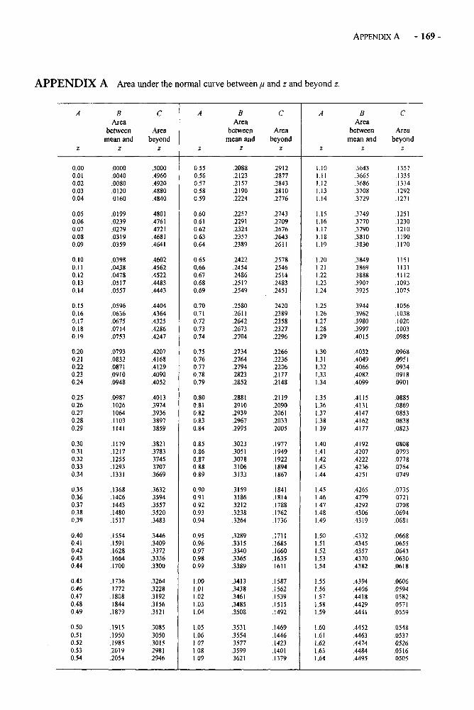
APPENDIX A Area under the normal curve between u and z and beyond z.
APPENDIX A -169 -
0.000.010.020.030.04
0.050.060.070.080.09
0.100.110.120.130.14
0.150.160.170.180.19
0.200.210.220.230.24
0.250.260.270.280.29
0.300.310.320.330.34
0.350.360.370.380.39
0.400.410.420.430.44
0.450.460.470.480.49
0.500.510.520.530.54
BArea
betweenmean and
z
.0000
.0040
.0080
.0120
.0160
.0199
.0239
.0279
.0319
.0359
.0398
.0438
.0478
.0517
.0557
.0596
.0636
.0675
.0714
.0753
.0793
.0832
.0871
.0910
.0948
.0987
.1026
.1064
.1103
.1141
.1179
.1217
.1255
.1293
.1331
.1368
.1406
.1443
.1480
.1517
.1554
.1591
.1628
.1664
.1700
.1736
.1772
.1808
.1844
.1879
.1915
.1950
.1985
.2019
.2054
C
Areabeyondz
.5000
.4960
.4920
.4880
.4840
.4801
.4761
.4721
.4681
.4641
.4602
.4562
.4522
.4483
.4443
.4404
.4364
.4325
.4286
.4247
.4207
.4168
.4129
.4090
.4052
.4013
.3974
.3936
.3897
.3859
.3821
.3783
.3745
.3707
.3669
.3632
.3594
.3557
.3520
.3483
.3446
.3409
.3372
.3336
.3300
.3264
.3228
.3192
.3156
.3121
.3085
.3050
.3015
.2981
.2946
A
z
0.550.560.570.580.59
0.600.610.620.630.64
0.650.660.670.680.69
0.700.710.720.730.74
0.750.760.770.780.79
0.800.810.820.830.84
0.850.860.870.880.89
0.900.910.920.930.94
0.950.960.970.980.99
1.001.011.021.031.04
1.051.061.071.081.09
BArea
betweenmean and
z
.2088
.2123
.2157
.2190
.2224
.2257
.2291
.2324
.2357
.2389
.2422
.2454
.2486
.2517
.2549
.2580
.2611
.2642
.2673
.2704
.2734
.2764
.2794
.2823
.2852
.2881
.2910
.2939
.2967
.2995
.3023
.3051
.3078
.3106
.3133
.3159
.3186
.3212
.3238
.3264
.3289
.3315
.3340
.3365
.3389
.3413
.3438
.3461
.3485
.3508
.3531
.3554
.3577
.3599
.3621
C
Areabeyond
z
.2912
.2877
.2843
.2810
.2776
.2743
.2709
.2676
.2643
.2611
.2578
.2546
.2514
.2483
.2451
.2420
.2389
.2358
.2327
.2296
.2266
.2236
.2206
.2177
.2148
.2119
.2090
.2061
.2033
.2005
.1977
.1949
.1922
.1894
.1867
.1841
.1814
.1788
.1762
.1736
.1711
.1685
.1660
.1635
.1611
.1587
.1562
.1539
.1515
.1492
.1469
.1446
.1423
.1401
.1379
A
z
1.101 . 1 11.121.131.14
1.151.161.171.181.19
1.201.211.221.231.24
1.251.261.271.281.29
1.301.311.321.331.34
1.351.36.37.38.39
.40
.41
.42
.43
.44
.45
.46
.47
.481.49
1.50.51.52.53.54
.55
.56
.57
.58
.59
.60
.61
.621.631.64
BArea
betweenmean and
z
.3643
.3665
.3686
.3708
.3729
.3749
.3770
.3790
.3810
.3830
.3849
.3869
.3888
.3907
.3925
.3944
.3962
.3980
.3997
.4015
.4032
.4049
.4066
.4082
.4099
.4115
.4131
.4147
.4162
.4177
.4192
.4207
.4222
.4236
.4251
.4265
.4279
.4292
.4306
.4319
.4332
.4345
.4357
.4370
.4382
.4394
.4406
.4418
.4429
.4441
.4452
.4463
.4474
.4484
.4495
C
Areabeyondz
.1357
.1335
.1314
.1292
.1271
.1251
.1230
.1210
.1190
.1170
11511131. 1 1 1 2.1093.1075
.1056
.1038
.1020
.1003
.0985
.0968
.0951
.0934
.0918
.0901
.0885
.0869
.0853
.0838
.0823
.0808
.0793
.0778
.0764
.0749
.07350721.0708.0694.0681
.0668
.0655
.0643
.0630
.0618
.0606
.05940582.0571.0559
.0548
.0537
.0526
.0516
.0505
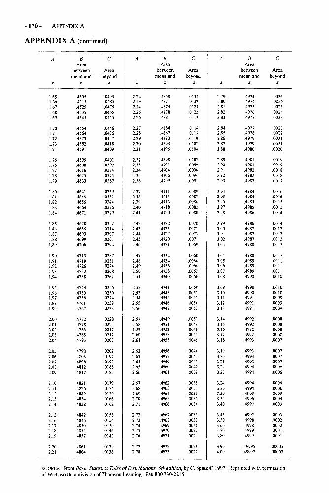
-170- APPENDIX A
APPENDIX A (continued)
A
z
1.651.661.671.681.69
1.701.711.721.731.74
1.751.761.771.781.79
1.801.811.821.831.84
1.851.861.871.881.89
1.901.911.92.93.94
.95
.96
.97
.981.99
2.002.012.022.032.04
2.052.062.072.082.09
2.102.112.122.132.14
2.152.162.172.182.19
2.202.21
BArea
betweenmean and
z
.4505
.4515
.4525
.4535
.4545
.4554
.4564
.4573
.4582
.4591
.4599
.4608
.4616
.4625
.4633
.4641
.4649
.4656
.4664
.4671
.4678
.4686
.4693
.4699
.4706
.4713
.4719
.4726
.4732
.4738
.4744
.4750
.4756
.4761
.4767
.4772
.4778
.4783
.4788
.4793
.4798
.4803
.4808
.4812
.4817
.4821
.4826
.4830
.4834
.4838
.4842
.4846
.4850
.4854
.4857
.4861
.4864
C
Areabeyondz
.0495
.0485
.0475
.0465
.0455
.0446
.0436
.0427
.0418
.0409
.0401
.0392
.0384
.0375
.0367
.0359
.0351
.0344
.0336
.0329
.0322
.0314
.0307
.0301
.0294
.0287
.0281
.0274
.0268
.0262
.0256
.0250
.0244
.0239
.0233
.0228
.0222
.0217
.0212
.0207
.0202
.0197
.0192
.0188
.0183
.0179
.0174
.0170
.0166
.0162
.0158
.0154
.0150
.0146
.0143
.0139
.0136
A
z
2.222.232.242.252.26
2.272.282.292.302.31
2.322.332.342.352.36
2.372.382.392.402.41
2.422.432.442.452.46
2.472.482.492.502.51
2.522.532.542.552.56
2.572.582.592.602.61
2.622.632.642.652.66
2.672.682.692.702.71
2.722.732.742.752.76
2.772.78
BArea
betweenmean and
z
.4868
.4871
.4875
.4878
.4881
.4884
.4887
.4890
.4893
.4896
.4898
.4901
.4904
.4906
.4909
.4911
.4913
.4916
.4918
.4920
.4922
.4925
.4927
.4929
.4931
.4932
.4934
.4936
.4938
.4940
.4941
.4943
.4945
.4946
.4948
.4949
.4951
.4952
.4953
.4955
.4956
.4957
.4959
.4960
.4961
.4962
.4963
.4964
.4965
.4966
.4967
.4968
.4969
.4970
.4971
.4972
.4973
C
Areabeyond
z
.0132
.0129
.0125
.0122
.0119
.0116
.0113
.0110
.0107
.0104
.0102
.0099
.0096
.0094
.0091
.0089
.0087
.0084
.0082
.0080
.0078
.0075
.0073
.0071
.0069
.0068
.0066
.0064
.0062
.0060
.0059
.0057
.0055
.0054
.0052
.0051
.0049
.0048
.0047
.0045
.0044
.0043
.0041
.0040
.0039
.0038
.0037
.0036
.0035
.0034
.0033
.0032
.0031
.0030
.0029
.0028
.0027
A
z
2.792.802.812.822,83
2.842.852.862.872.88
2.892.902.912.922.93
2.942.952.962.972.98
2.993.003.013.023.03
3.043.053.063.073.08
3.093.103.113.123.13
3.143.153.163.173.18
3.193.203.213.223.23
3.243.253.303.353.40
3.453.503.603.703.80
3.904.00
BArea
betweenmean and
z
.4974
.4974
.49754976.4977
.4977
.4978
.4979
.4979
.4980
.4981
.4981
.4982
.4982
.4983
.4984
.4984
.4985
.4985
.4986
.4986
.4987
.4987
.4987
.4988
.4988
.4989
.4989
.4989
.4990
.4990
.4990
.4991
.4991
.4991
.4992
.4992
.4992
.4992
.4993
.4993
.4993
.4993
.4994
.4994
.4994
.4994
.4995
.4996
.4997
.4997
.4998
.49984999.4999
.49995
.49997
C
Areabeyondz
00260026.002500240023
.0023
.0022
.0021
.0021
.0020
.00190019.001800180017
.0016
.0016
.0015
.0015
.0014
.0014
.00130013.00130012
00120011.0011.0011.0010
.0010
.0010
.00090009.0009
.000800080008.0008.0007
.0007
.0007
.0007
.0006
.0006
0006000600050004.0003
.0003
.0002
.0002
.0001
.0001
.00005
.00003
SOURCE: From Basic Statistics Tales of Distributions, 6th edition, by C. Spatz © 1997. Reprinted with permissionof Wadsworth, a division of Thomson Learning. Fax 800 730-2215.
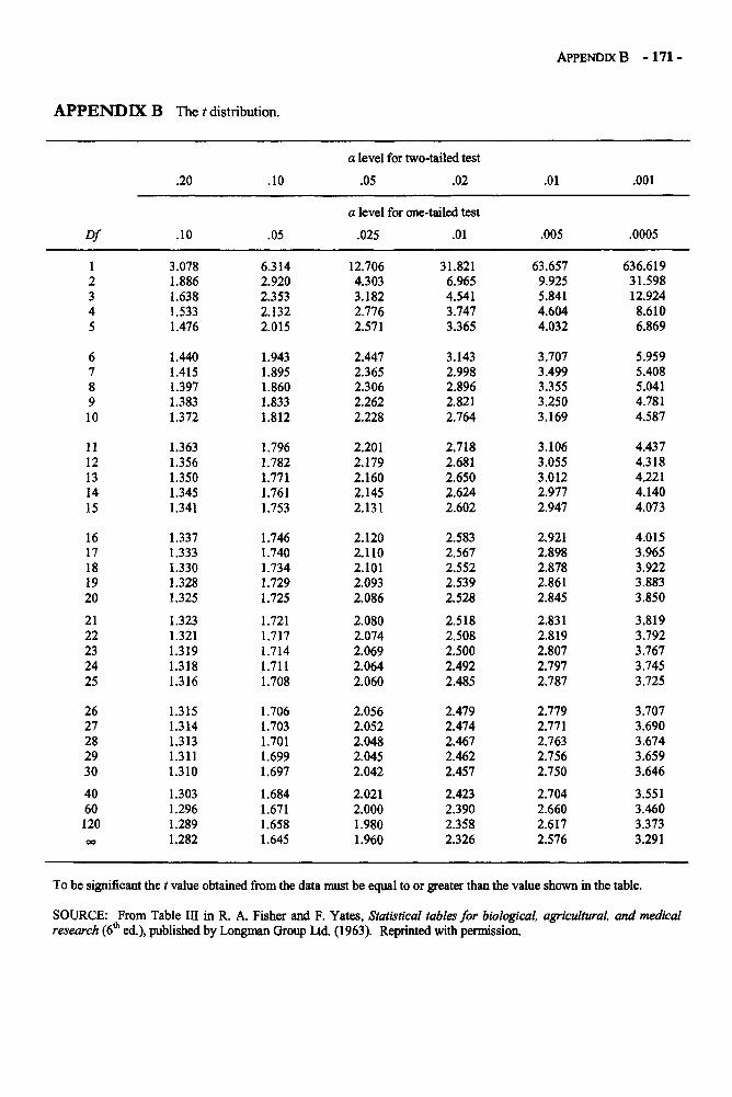
APPENDIX B The t distribution.
APPENDIX B -171 -
.20 .10
a level for two-tailed test
.05 .02 .01 .001
Df
12345
678910
1112131415
1617181920
2122232425
2627282930
4060120
.10
3.0781.8861.6381.5331.476
1.4401.4151.3971.3831.372
1.3631.3561.3501.3451.341
1.3371.3331.3301.3281.325
1.3231.3211.3191.3181.316
1.3151.3141.3131.3111.310
1.3031.2961.2891.282
.05
6.3142.9202.3532.1322.015
1.9431.8951.8601.8331.812
1.7961.7821.7711.7611.753
1.7461.7401.7341.7291.725
1.7211.7171.7141.7111.708
1.7061.7031.7011.6991.697
1.6841.6711.6581.645
a level for one-tailed test
.025 .01
12.7064.3033.1822.7762.571
2.4472.3652.3062.2622.228
2.2012.1792.1602.1452.131
2.1202.1102.1012.0932.086
2.0802.0742.0692.0642.060
2.0562.0522.0482.0452.042
2.0212.0001.9801.960
31.8216.9654.5413.7473.365
3.1432.9982.8962.8212.764
2.7182.6812.6502.6242.602
2.5832.5672.5522.5392.528
2.5182.5082.5002.4922.485
2.4792.4742.4672.4622.457
2.4232.3902.3582.326
.005
63.6579.9255.8414.6044.032
3.7073.4993.3553.2503.169
3.1063.0553.0122.9772.947
2.9212.8982.8782.8612.845
2.8312.8192.8072.7972.787
2.7792.7712.7632.7562.750
2.7042.6602.6172.576
.0005
636.61931.59812.9248.6106.869
5.9595.4085.0414.7814.587
4.4374.3184.2214.1404.073
4.0153.9653.9223.8833.850
3.8193.7923.7673.7453.725
3.7073.6903.6743.6593.646
3.5513.4603.3733.291
To be significant the t value obtained from the data must be equal to or greater than the value shown in the table.
SOURCE: From Table III in R. A. Fisher and F. Yates, Statistical tables for biological, agricultural, and medicalresearch (6th ed.), published by Longman Group Ltd. (1963). Reprinted with permissioa
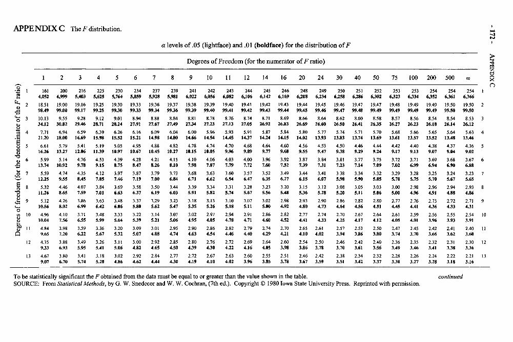
APPENDIX C The F distribution.
a levels of .05 (lightface) and .01 (boldface) for the distribution of F
Degrees of Freedom (for the numerator of F ratio)
2.
0
1
2
3
4
5
6
7
8
9
10
11
12
13
1
1614,052
18.5198.49
10.1334.12
7.7121.20
6.6116.26
5.9913.74
5.5912.25
5.3211.26
5.1210.56
4.9610.04
4.849.65
4.759.33
4.679.07
2
2004,999
19.0099.00
9.5530.82
6.9418.00
5.7913.27
5.1410.92
4.749.55
4.468.65
4.268.02
4.107.56
3.987.20
3.886.93
3.806.70
3
2165,403
19.1699.17
9.2829.46
6.5916.69
5.4112.06
4.769.78
4.358.45
4.077.59
3.866.99
3.716.55
3.596.22
3.495.95
3.415.74
4
2255,625
19.2599.25
9.1228.71
6.3915.98
5.1911.39
4.539.15
4.127.85
3.847.01
3.636.42
3.485.99
3.365.67
3.265.41
3.185.20
5
2305,764
19.3099.30
9.0128.24
6.2615.52
5.0510.97
4.398.75
3.977.46
3.696.63
3.486.06
3.335.64
3.205.32
3.115.06
3.024.86
6
2345,859
19.339933
8.9427.91
6.1615.21
4.9510.67
4.288.47
3.877.19
3.586.37
3.375.80
3.225.39
3.095.07
3.004.82
2.924.62
7
2375,928
19.369934
8.8827.67
6.0914.98
4.8810.45
4.218.26
3.797.00
3.506.19
3.295.62
3.145.21
3.014.88
2.924.65
2.844.44
8
2395,981
19.3799.36
8.8427.49
6.0414.80
4.8210.27
4.158.10
3.736.84
3.446.03
3.235.47
3.075.06
2.954.74
2.854.50
2.774.30
9
2416,022
19.389939
8.812734
6.0014.66
4.7810.15
4.107.98
3.686.71
3.395.91
3.185.35
3.024.95
2.904.63
2.804.39
2.724.19
10
2426,056
19.3999.40
8.7827.23
5.9614.54
4.7410.05
4.067.87
3.636.62
3.345.82
3.135.26
2.974.85
2.864.54
2.764.30
2.674.10
11
2436,082
19.4099.41
8.7627.13
5.9314.45
4.709.96
4.037.79
3.606.54
3.315.74
3.105.18
2.944.78
2.824.46
2.724.22
2.634.02
12
2446,106
19.4199.42
8.7427.05
5.911437
4.689.89
4.007.72
3.576.47
3.285.67
3.075.11
2.914.71
2.794.40
2.694.16
2.603.96
14
2456,142
19.4299.43
8.7126.92
5.8714.24
4.649.77
3.967.60
3.526.35
3.235.56
3.025.00
2.864.60
2.744.29
2.644.05
2.553.85
16
2466,169
19.4399.44
8.6926.83
5.8414.15
4.609.68
3.927.52
3.496.27
3.205.48
2.984.92
2.824.52
2.704.21
2.603.98
2.513.78
20
2486,208
19.4499.45
8.6626.69
5.8014.02
4.569.55
3.87739
3.446.15
3.15536
2.934.80
2.774.41
2.654.10
2.543.86
2.463.67
24
2496,234
19.4599.46
8.6426.60
5.7713.93
4.539.47
3.84731
3.416.07
3.125.28
2.904.73
2.744.33
2.614.02
2.503.78
2.423.59
30
2506,258
19.4699.47
8.6226.50
5.7413.83
4.509.38
3.817.23
3.385.98
3.085.20
2.864.64
2.704.25
2.573.94
2.463.70
2.383.51
40
2516,286
19.4799.48
8.6026.41
5.7113.74
4.469.29
3.777.14
3.345.90
3.055.11
2.824.56
2.674.17
2.533.86
2.423.61
2.343.42
50
2526302
19.4799.49
8.582635
5.7013.69
4.449.24
3.757.09
3.325.85
3.035.06
2.804.51
2.644.12
2.503.80
2.403.56
2.323.37
75
2536323
19.4899.49
8.5726.27
5.6813.61
4.429.17
3.727.02
3.295.78
3.005.00
2.774.45
2.614.05
2.473.74
2.363.49
2.283.30
100
2536334
19.4999.49
8.5626.23
5.6613.57
4.409.13
3.716.99
3.285.75
2.984.96
2.764.41
2.594.01
2.453.70
2.353.46
2.263.27
200
2546352
19.4999.49
8.5426.18
5.6513.52
4.389.07
3.696.94
3.255.70
2.964.91
2.734.36
2.563.96
2.423.66
2.323.41
2.243.28
500
2546361
19.5099.50
8.5426.14
5.6413.48
4.379.04
3.686.90
3.245.67
2.944.88
2.72433
2.553.93
2.413.62
2.31338
2.223.18
00
2546366
19.5099.50
8.5326.12
5.6313.46
4.369.02
3.676.88
3.235.65
2.934.86
2.71431
2.543.91
2.403.60
2.30336
2.213.16
1
2
3
4
5
6
7
8
9
10
11
12
13
To be statistically significant the F obtained from the data must be equal to or greater than the value shown in the table.SOURCE: From Statistical Methods, by G. W. Snedecor and W. W. Cochran, (7th ed.). Copyright © 1980 Iowa State University Press. Reprinted with permission.
continued

APPENDIX C (continued)
Degrees of Freedom (for the numerator of F ratio)
'1
03C
&
\4
\5
\6
18
19
20
21
22
23
24
25
26
1
4.608.86
4.548.68
4.498.53
4.458.40
4.418.28
4.388.18
4.358.10
4.328.02
4.307.94
4.287.88
4.267.82
4.247.77
4.227.72
2
3.746.51
3.686.36
3.636.23
3.596.11
3.556.01
3.525.93
3.495.85
3.475.78
3.445.72
3.425.66
3.405.61
3.385.57
3.375.53
3
3.345.56
3.295.52
3.245.29
3.205.18
3.165.09
3.135.01
3.104.94
3.074.87
3.054.82
3.034.76
3.014.72
2.994.68
2.984.64
4
3.115.03
3.064.89
3.014.77
2.964.67
2.934.58
2.904.50
2.874.43
2.844.37
2.824.31
2.804.26
2.784.22
2.764.18
2.744.14
5
2.964.69
2.904.56
2.854.44
2.814.34
2.774.25
2.744.17
2.714.10
2.684.04
2.663.99
2.643.94
2.623.90
2.603.86
2.593.82
6
2.854.46
2.794.32
2.744.20
2.704.10
2.664.01
2.633.94
2.603.87
2.573.81
2.553.76
2.533.71
2.513.67
2.493.63
2.473.59
7
2.774.28
2.704.14
2.664.03
2.623.93
2.583.85
2.553.77
2.523.71
2.493.65
2.473.59
2.453.54
2.433.50
2.413.46
2.393.42
8
2.704.14
2.644.00
2.593.89
2.553.79
2.513.71
2.483.63
2.453.56
2.423.51
2.403.45
2.383.41
2.363.36
2.343.32
2.323.29
9
2.654.03
2.593.89
2.543.78
2.503.68
2.463.60
2.433.52
2.403.45
2.373.40
2.353.35
2.323.30
2.303.25
2.283.21
2.273.17
10
2.603.94
2.553.80
2.493.69
2.453.59
2.413.51
2.383.43
2.353.37
2.323.31
2.303.26
2.283.21
2.263.17
2.243.13
2.223.09
11
2.563.86
2.513.73
2.453.61
2.413.52
2.373.44
2.343.36
2.313.30
2.283.24
2.263.18
2.243.14
2.223.09
2.203.05
2.183.02
12
2.533.80
2.483.67
2.423.55
2.383.45
2.343.37
2.313.30
2.283.23
2.253.17
2.233.12
2.203.07
2.183.03
2.162.99
2.152.96
14
2.483.70
2.433.56
2.373.45
2.333.35
2.293.27
2.263.19
2.233.13
2.203.07
2.183.02
2.142.97
2.132.93
2.112.89
2.102.86
16
2.443.62
2.393.48
2.333.37
2.293.27
2.253.19
2.213.12
2.183.05
2.152.99
2.132.94
2.102.89
2.092.85
2.062.81
2.052.77
20
2.393.51
2.333.36
2.283.25
2.233.16
2.193.07
2.153.00
2.122.94
2.092.88
2.072.83
2.042.78
2.022.74
2.002.70
1.992.66
24
2.353.43
2.293.29
2.243.18
2.193.08
2.153.00
2.112.92
2.082.86
2.052.80
2.032.75
2.002.70
1.982.66
1.962.62
1.952.58
30
2.313.34
2.253.20
2.203.10
2.153.00
2.112.91
2.072.84
2.042.77
2.002.72
1.982.67
1.962.62
1.942.58
1.922.54
1.902.50
40
2.273.26
2.213.12
2.163.01
2.112.92
2.072.83
2.022.76
1.992.69
1.962.63
1.932.58
1.912.53
1.892.49
1.872.45
1.852.41
50
2.243.21
2.183.07
2.132.96
2.082.86
2.042.78
2.002.70
1.962.63
1.932.58
1.912.53
1.882.48
1.862.44
1.842.40
1.822.36
75
2.213.14
2.153.00
2.092.98
2.042.79
2.002.71
1.962.63
1.922.56
1.892.51
1.872.46
1.842.41
1.822.36
1.802.32
1.782.28
100
2.193.11
2.122.97
2.072.86
2.022.76
1.892.68
1.942.60
1.902.53
1.872.47
1.842.42
1.822.37
1.802.33
1.772.29
1.762.25
200
2.163.06
2.102.92
2.042.80
1.992.70
1.952.62
1.912.54
1.872.47
1.842.42
1.812.37
1.792.32
1.762.27
1.742.23
1.722.19
500
2.143.02
2.082.89
2.022.77
1.972.67
1.932.59
1.902.51
1.852.44
1.822.38
1.802.33
1.772.28
1.742.23
1.722.19
1.702.15
00
2.133.00
2.072.87
2.012.75
1.962.65
1.922.57
1.882.49
1.842.42
1.812.36
1.782.31
1.762.26
1.732.21
1.712.17
1.692.13
contfrtwed
14
15
16
17
18
19
20
21
22
23
24
25
26
>
X
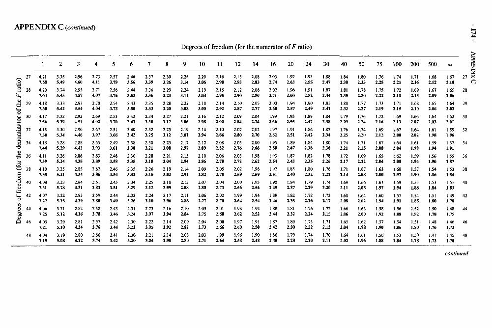
APPENDIX C (continued)
Degrees of freedom (for the numerator of F ratio)
'i
CO
27
28
29
30
32
34
36
38
40
42
44
46
48
1
4.217.68
4.207.64
4.187.60
4.177.56
4.157.50
4.137.44
4.117.39
4.107.35
4.087.31
4.077.27
4.067.25
4.057.21
4.047.19
2
3.355.49
3.345.45
3.335.42
3.325.39
3.305.34
3.285.29
3.265.24
3.255.21
3.235.18
3.225.15
3.215.12
3.205.10
3.195.08
3
2.964.60
2.954.57
2.934.54
2.924.51
2.904.46
2.884.42
2.864.38
2.854.34
2.844.31
2.834.29
2.824.26
2.814.24
2.804.22
4
2.734.11
2.714.07
2.704.04
2.694.02
2.673.97
2.653.93
2.633.89
2.623.86
2.613.83
2.593.80
2.583.78
2.573.76
2.563.74
5
2.573.79
2.563.76
2.543.73
2.533.70
2.513.66
2.493.61
2.483.58
2.463.54
2.453.51
2.443.49
2.433.46
2.423.44
2.413.42
6
2.463.56
2.443.53
2.433.50
2.423.47
2.403.42
2.383.38
2.363.35
2.353.32
2.343.29
2.323.26
2.313.24
2.303.22
2.303.20
7
2.373.39
2.363.36
2.353.33
2.343.30
2.323.25
2.303.21
2.283.18
2.263.15
2.253.12
2.243.10
2.233.07
2.223.05
2.213.04
8
2.303.26
2.293.23
2.283.20
2.273.17
2.253.12
2.233.08
2.213.04
2.193.02
2.182.99
2.172.96
2.162.94
2.142.92
2.142.90
9
2.253.14
2.243.11
2.223.08
2.213.06
2.193.01
2.172.97
2.152.94
2.142.91
2.122.88
2.112.86
2.102.84
2.092.82
2.082.80
10
2.203.06
2.193.03
2.183.00
2.162.98
2.142.94
2.122.89
2.102.86
2.092.82
2.072.80
2.062.77
2.052.75
2.042.73
2.032.71
11
2.162.98
2.152.95
2.142.92
2.122.90
2.102.86
2.082.82
2.062.78
2.052.75
2.042.73
2.022.70
2.012.68
2.002.66
1.992.64
12
2.132.93
2.122.90
2.102.87
2.092.84
2.072.80
2.052.76
2.032.72
2.022.69
2.002.66
1.992.64
1.982.62
1.972.60
1.962.58
14
2.082.83
2.062.80
2.052.77
2.042.74
2.022.70
2.002.66
1.982.62
1.962.59
1.952.56
1.942.54
1.922.52
1.912.50
1.902.48
16
2.032.74
2.022.71
2.002.68
1.992.66
1.972.62
1.952.58
1.932.54
1.922.51
1.902.49
1.892.46
1.882.44
1.872.42
1.862.40
20
1.972.63
1.962.60
1.942.57
1.932.55
1.912.51
1.892.47
1.872.43
1.852.40
1.842.37
1.822.35
1.812.32
1.802.30
1.792.28
24
1.932.55
1.912.52
1.902.49
1.892.47
1.862.42
1.842.38
1.822.35
1.802.32
1.792.29
1.782.26
1.762.24
1.752.22
1.742.20
30
1.882.47
1.872.44
1.852.41
1.842.38
1.822.34
1.802.30
1.782.26
1.762.22
1.742.20
1.732.17
1.722.15
1.712.13
1.702.11
40
1.842.38
1.812.35
1.802.32
1.792.29
1.762.25
1.742.21
1.722.17
1.712.14
1.692.11
1.682.08
1.662.06
1.652.04
1.642.02
50
1.802.33
1.782.30
1.772.27
1.762.24
1.742.20
1.712.15
1.692.12
1.672.08
1.662.05
1.642.02
1.632.00
1.621.98
1.611.96
75
1.762.25
1.752.22
1.732.19
1.722.16
1.692.12
1.672.08
1.652.04
1.632.00
.61
.97
.60
.94
.58
.92
.57
.90
1.561.88
100
1.742.21
1.722.18
1.712.15
1.692.13
1.672.08
1.642.04
1.622.00
1.601.97
1.591.94
1.571.91
1.561.88
1.541.86
1.531.84
200
1.712.16
1.692.13
1.682.10
1.662.07
1.642.02
1.611.98
1.591.94
1.571.90
1.551.88
.54
.85
.52
.82
.51
.80
1.501.78
500
1.682.12
1.672.09
1.652.06
1.642.03
1.611.98
1.591.94
1.561.90
1.541.86
1.531.84
1.511.80
1.501.78
1.481.76
1.471.73
>
.67 27 X
.65 282.06
.64 292.03
.62 302.01
.59 321.96
.57 341.91
.55 36
.87
.53 38
.84
.51 40
.81
.49 42
.78
.48 44
.75
1.46 461.72
1.45 481.70
continued
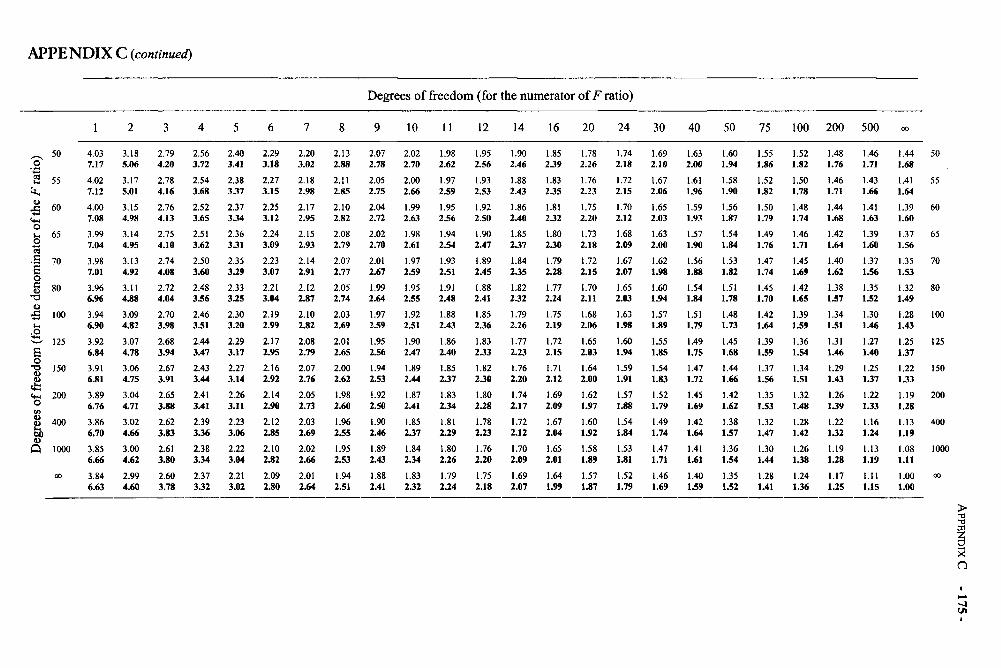
APPENDIX C (continued)
Degrees of freedom (for the numerator of F ratio)
10 11 12 14 16 20 24 30 40 50 75 100 200 500
50.22 55
60
65
70
80
100
£ 125
15°
200
400
1000
00
4.037.17
4.027.12
4.007.08
3.997.04
3.987.01
3.966.96
3.946.90
3.926.84
3.916.81
3.896.76
3.866.70
3.856.66
3.846.63
3.185.06
3.175.01
3.154.98
3.144.95
3.134.92
3.114.88
3.094.82
3.074.78
3.064.75
3.044.71
3.024.66
3.004.62
2.994.60
2.794.20
2.784.16
2.764.13
2.754.10
2.744.08
2.724.04
2.703.98
2.683.94
2.673.91
2.653.88
2.623.83
2.613.80
2.603.78
2.563.72
2.543.68
2.523.65
2.513.62
2.503.60
2.483.56
2.463.51
2.443.47
2.433.44
2.413.41
2.393.36
2.383.34
2.37332
2.403.41
2.383.37
2.373.34
2.363.31
2.353.29
2.333.25
2.303.20
2.293.17
2.273.14
2.263.11
2.233.06
2.223.04
2.213.02
2.293.18
2.273.15
2.253.12
2.243.09
2.233.07
2.213.04
2.192.99
2.172.95
2.162.92
2.142.90
2.122.85
2.102.82
2.092.80
2.203.02
2.182.98
2.172.95
2.152.93
2.142.91
2.122.87
2.102.82
2.082.79
2.072.76
2.052.73
2.032.69
2.022.66
2.012.64
2.132.88
2.112.85
2.102.82
2.082.79
2.072.77
2.052.74
2.032.69
2.012.65
2.002.62
1.982.60
1.962.55
1.952.53
1.942.51
2.072.78
2.052.75
2.042.72
2.022.70
2.012.67
1.992.64
1.972.59
1.952.56
1.942.53
1.922.50
1.902.46
1.892.43
1.882.41
2.022.70
2.002.66
1.992.63
1.982.61
1.972.59
1.952.55
1.922.51
1.902.47
1.892.44
1.872.41
1.852.37
1.842.34
1.832.32
1.982.62
1.972.59
1.952.56
1.942.54
1.932.51
1.912.48
1.882.43
1.862.40
1.85237
1.83234
1.812.29
1.802.26
1.792.24
1.952.56
1.932.53
1.922.50
1.902.47
1.892.45
1.882.41
1.852.36
1.83233
1.822.30
1.802.28
1.782.23
1.762.20
1.752.18
1.902.46
1.882.43
1.862.40
1.85237
1.842.35
1.82232
1.792.26
1.772.23
1.762.20
1.742.17
1.722.12
1.702.09
1.692.07
1.85239
1.83235
1.812.32
1.802.30
1.792.28
1.772.24
1.752.19
1.722.15
1.712.12
1.692.09
1.672.04
1.652.01
1.641.99
1.782.26
1.762.23
1.752.20
1.732.18
1.722.15
1.702.11
1.682.06
1.652.03
1.642.00
1.621.97
1.601.92
1.581.89
1.571.87
1.742.18
1.722.15
1.702.12
1.682.09
1.672.07
1.652.03
1.631.98
1.601.94
1.591.91
1.571.88
1.541.84
1.531.81
1.521.79
1.692.10
1.672.06
1.652.03
1.632.00
1.621.98
1.601.94
1.571.89
1.551.85
1.541.83
1.521.79
1.491.74
1.471.71
1.461.69
1.632.00
1.611.96
1.591.93
1.571.90
1.561.88
1.541.84
1.511.79
1.491.75
1.471.72
1.451.69
1.421.64
1.411.61
1.401.59
1.601.94
1.581.90
1.561.87
1.541.84
1.531.82
1.511.78
1.481.73
1.451.68
1.441.66
1.421.62
1.381.57
1.361.54
1.351.52
.55
.86
.52
.82
.50
.79
.49
.76
.47
.74
.45
.70
.42
.64
.39
.59
.37
.56
.35
.53
.32
.47
.30
.44
1.281.41
1.521.82
1.501.78
1.481.74
1.461.71
1.451.69
1.421.65
1.391.59
1.361.54
1.341.51
1.321.48
1.281.42
1.26138
1.241.36
1.481.76
1.461.71
1.441.68
1.421.64
1.401.62
1.381.57
1.341.51
1.311.46
1.291.43
1.26139
1.22132
1.191.28
1.171.25
1.461.71
1.431.66
1.411.63
1.391.60
1.371.56
1.351.52
1.301.46
1.271.40
1.25137
1.22133
1.161.24
1.131.19
1.111.15
1.441.68
1.411.64
.39
.60
.37
.56
.35
.53
1.321.49
1.281.43
1.251.37
1.22133
1.191.28
.13
.19
.08
.11
.00
.00
50
55
60
65
70
80
100
125
150
200
400
1000
00
>
X

APPENDIX D Critical values of the studentized range statistic (for Tukey HSD tests).
a = .05
Number of levels of the independent variable
dferror
12345678910111213141516171819202430406012000
2
17.976.084.503.933.643.463.343.263.203.153.113.083.063.033.013.002.982.972.962.952.922.892.862.832.802.77
3
26.988.335.915.044.604.344.164.043.953.883.823.773.743.703.673.653.633.613.593.583.533.493.443.403.363.31
4
2.829.806.825.765.224.904.684.534.424.334.264.204.154.114.084.054.024.003.983.963.903.843.793.743.693.63
5
37.0710.887.506.295.675.315.064.894.764.654.574.514.454.414.374.334.304.284.254.234.174.104.043.983.923.86
6
40.4111.748.046.716.035.635.365.175.024.914.824.754.694.644.604.564.524.504.474.444.374.304.234.164.104.03
7
43.1212.448.487.056.335.905.615.405.245.125.034.954.884.834.784.744.704.674.644.624.544.464.394.314.244.17
8
45.4013.038.857.356.586.125.825.605.435.305.205.125.054.994.944.904.864.824.794.774.684.604.524.444.364.29
9
47.3613.549.187.606.806.326.005.775.605.465.355.265.195.135.085.034.994.964.924.904.814.724.644.554.474.39
10
49.0713.999.467.337.006.496.165.925.745.605.495.405.325.255.205.155.115.075.045.014.924.824.744.654.564.47
11
50.5914.399.728.037.176.656.306.055.875.725.605.515.435.365.315.265.215.175.145.115.014.924.824.734.644.55
12
51.9614.759.958.217.326.796.436.185.985.835.715.625.535.465.405.355.315.275.235.205.105.004.904.814.714.62
13
53.2015.0810.158.377.476.926.556.296.095.945.815.715.635.555.495.445.395.355.325.285.185.084.984.884.784.68
14
54.3315.3810.358.527.607.036.666.396.196.035.905.795.715.645.575.525.475.435.395.365.255.155.044.944.844.74
15
55.3615.6510.538.667.727.146.766.486.286.115.985.885.795.715.655.595.545.505.465.435.325.215.115.004.904.80
SOURCE: From "Tables of Range and Studentized Range," by M. L. Harter, Annals of Mathematical Statistics, 31, 1122-1147 (1960). Reprinted with permission.
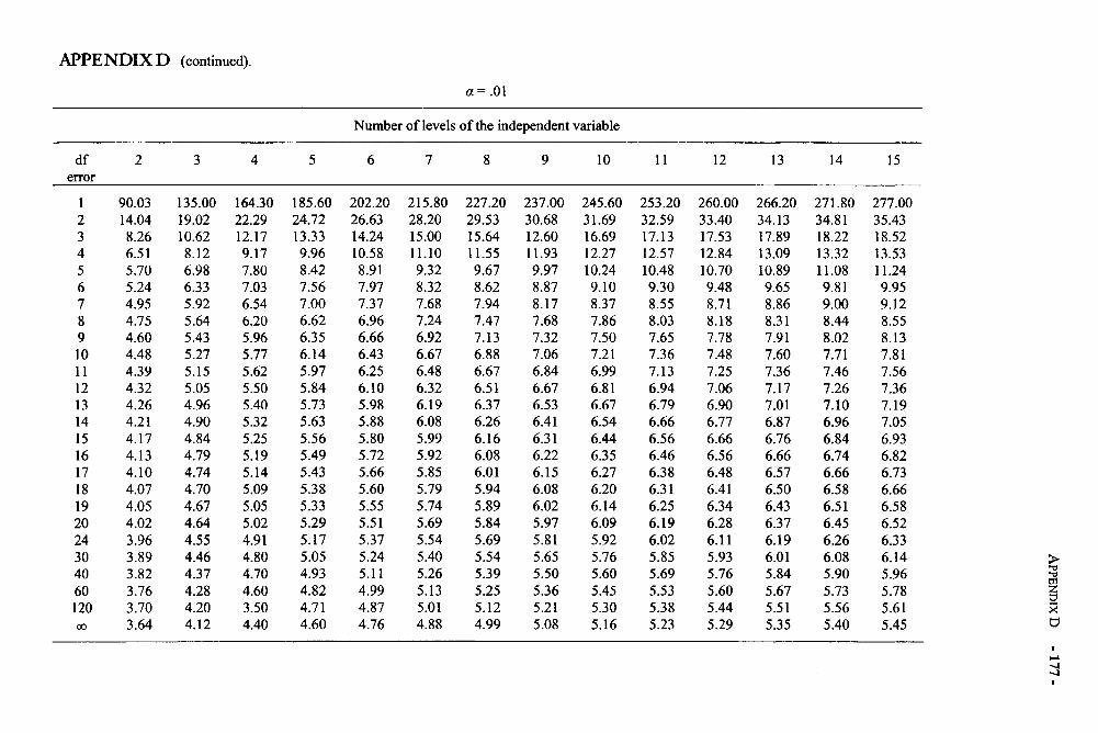
APPENDIX D (continued).
a = .01
Number of levels of the independent variable
dferror
12345678910111213141516171819202430406012000
2
90.0314.048.266.515.705.244.954.754.604.484.394.324.264.214.174.134.104.074.054.023.963.893.823.763.703.64
3
135.0019.0210.628.126.986.335.925.645.435.275.155.054.964.904.844.794.744.704.674.644.554.464.374.284.204.12
4
164.3022.2912.179.177.807.036.546.205.965.775.625.505.405.325.255.195.145.095.055.024.914.804.704.603.504.40
5
185.6024.7213.339.968.427.567.006.626.356.145.975.845.735.635.565.495.435.385.335.295.175.054.934.824.714.60
6
202.2026.6314.2410.588.917.977.376.966.666.436.256.105.985.885.805.725.665.605.555.515.375.245.114.994.874.76
7
215.8028.2015.0011.109.328.327.687.246.926.676.486.326.196.085.995.925.855.795.745.695.545.405.265.135.014.88
8
227.2029.5315.6411.559.678.627.947.477.136.886.676.516.376.266.166.086.015.945.895.845.695.545.395.255.124.99
9
237.0030.6812.6011.939.978.878.177.687.327.066.846.676.536.416.316.226.156.086.025.975.815.655.505.365.215.08
10
245.6031.6916.6912.2710.249.108.377.867.507.216.996.816.676.546.446.356.276.206.146.095.925.765.605.455.305.16
11
253.2032.5917.1312.5710.489.308.558.037.657.367.136.946.796.666.566.466.386.316.256.196.025.855.695.535.385.23
12
260.0033.4017.5312.8410.709.488.718.187.787.487.257.066.906.776.666.566.486.416.346.286.115.935.765.605.445.29
13
266.2034.1317.8913.0910.899.658.868.317.917.607.367.177.016.876.766.666.576.506.436.376.196.015.845.675.515.35
14
271.8034.8118.2213.3211.089.819.008.448.027.717.467.267.106.966.846.746.666.586.516.456.266.085.905.735.565.40
15
277.0035.4318.5213.5311.249.959.128.558.137.817.567.367.197.056.936.826.736.666.586.526.336.145.965.785.615.45
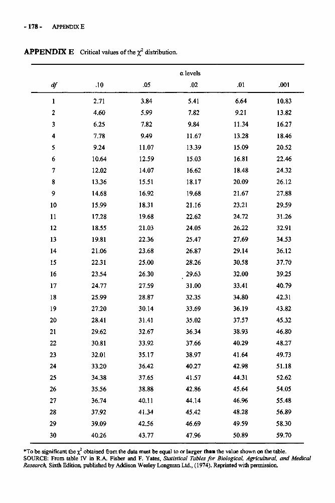
-178 - APPENDIX E
APPENDIX E Critical values of the x2 distribution.
df
1
2
3
4
5
6
7
8
9
10
11
12
13
14
15
16
17
18
19
20
21
22
23
24
25
26
27
28
29
30
.10
2.71
4.60
6.25
7.78
9.24
10.64
12.02
13.36
14.68
15.99
17.28
18.55
19.81
21.06
22.31
23.54
24.77
25.99
27.20
28.41
29.62
30.81
32.01
33.20
34.38
35.56
36.74
37.92
39.09
40.26
.05
3.84
5.99
7.82
9.49
11.07
12.59
14.07
15.51
16.92
18.31
19.68
21.03
22.36
23.68
25.00
26.30
27.59
28.87
30.14
31.41
32.67
33.92
35.17
36.42
37.65
38.88
40.11
41.34
42.56
43.77
a levels
.02
5.41
7.82
9.84
11.67
13.39
15.03
16.62
18.17
19.68
21.16
22.62
24.05
25.47
26.87
28.26
29.63
31.00
32.35
33.69
35.02
36.34
37.66
38.97
40.27
41.57
42.86
44.14
45.42
46.69
47.96
.01
6.64
9.21
11.34
13.28
15.09
16.81
18.48
20.09
21.67
23.21
24.72
26.22
27.69
29.14
30.58
32.00
33.41
34.80
36.19
37.57
38.93
40.29
41.64
42.98
44.31
45.64
46.96
48.28
49.59
50.89
.001
10.83
13.82
16.27
18.46
20.52
22.46
24.32
26.12
27.88
29.59
31.26
32.91
34.53
36.12
37.70
39.25
40.79
42.31
43.82
45.32
46.80
48.27
49.73
51.18
52.62
54.05
55.48
56.89
58.30
59.70
*To be significant the x2 obtained from the data must be equal to or larger than the value shown on the table.SOURCE: From table IV in R.A. Fisher and F. Yates, Statistical Tables for Biological, Agricultural, and MedicalResearch, Sixth Editioa published by Addison Wesley Longman Ltd., (1974). Reprinted with permission.
REFERENCES -179 -
REFERENCES
Aiken, L. S., & West, S. G. (1991). Multiple regression: Testing and interpreting interactions.Newbury Park, CA: Sage.
Berliner, D. C., & Biddle, B. J. (1995). The manufactured crisis: Myths, fraud, and the attack onAmerica's public schools. New York: Addison-Wesley.
Berry, W. D., & Feldman, S. (1985). Multiple regression in practice. Beverly Hills, CA: Sage.Bracey, G. W. (1991 5 October). Why can't they be like we were? Phi Delta Kappan (October),
104-117.Cohen, J., & Cohen, P. (1975). Applied multiple regression/correlation analysis for the behavioral
sciences. Hillsdale, NJ: Lawrence Erlbaum Associates.Glass, G. V., & Hopkins, K. D. (1996). Statistical methods in education and psychology (3rd ed.).
Boston: Allyn & Bacon.Hinkle, D. E., Wiersma, W., & Jurs, S. G. (1998). Applied statistics for the behavioral sciences (4th
ed.). Boston: Houghton Mifflin.Iverson, G. R., & Norpoth, H. (1987). Analysis of variance (2nd ed.) Newbury Park, CA: Sage.Jaccard, J., Turrisi, R., & Wan, C. K. (1990). Interaction effects in multiple regression. Newbury
Park, CA: Sage.Marascuilo, L. A., & Serlin, R. C. (1988). Statistical methods for the social and behavioral sciences.
New York: Freeman.Midgley, C., Kaplan, A., Middleton, M, et al. (1998). The development and validation of scales
assessing students' achievement goal orientations. Contemporary Educational Psychology,23, 113-131.
Mohr, L. B. (1990). Understanding significance testing. Newbury Park, CA: Sage.Naglieri, J.A. (1996). The Naglieri nonverbal ability test. San Antonio, TX: Harcourt Brace.Pedhazur, E. J. (1982). Multiple regression in behavioral research: Explanation and prediction
(2nd ed.). New York: Harcourt Brace.Spate, C. (2001). Basic statistics: Tales of distributions (7th ed.). Belmont, CA: Wadsworth.Wildt, A. R., & Ahtola, O. T. (1978). Analysis of covariance. Beverly Hills, CA: Sage.
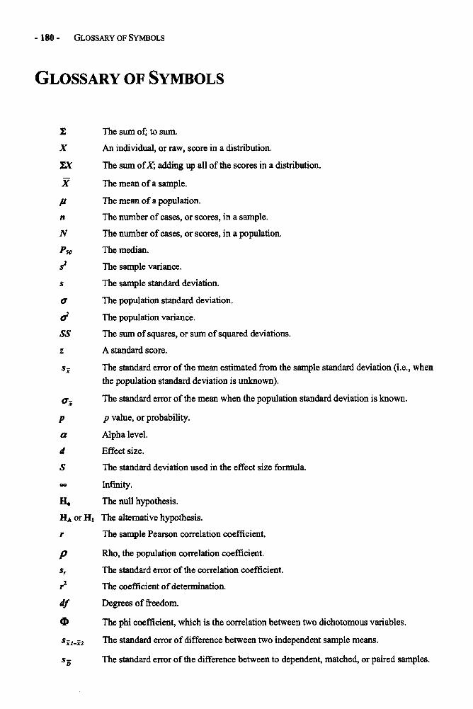
-180 - GLOSSARY OF SYMBOLS
GLOSSARY OF SYMBOLS
E The sum of; to sum.
X An individual, or raw, score in a distribution.
EX The sum of X; adding up all of the scores in a distribution.
X The mean of a sample.
u The mean of a population.
n The number of cases, or scores, in a sample.
N The number of cases, or scores, in a population.
P50 The median.
s2 The sample variance.
s The sample standard deviation.
a The population standard deviation.
o2 The population variance.
SS The sum of squares, or sum of squared deviations.
z A standard score.
Sx The standard error of the mean estimated from the sample standard deviation (i.e., whenthe population standard deviation is unknown).
ox The standard error of the mean when the population standard deviation is known.
p p value, or probability.
a Alpha level.
d Effect size.
S The standard deviation used in the effect size formula.
Infinity.
Ho The null hypothesis.
HA or H1 The alternative hypothesis.
r The sample Pearson correlation coefficient.
p Rho, the population correlation coefficient.
sr The standard error of the correlation coefficient.
r2 The coefficient of determination.
df Degrees of freedom.
The phi coefficient, which is the correlation between two dichotomous variables.
Sx1-x2 The standard error of difference between two independent sample means.
The standard error of the difference between to dependent, matched, or paired samples.SD
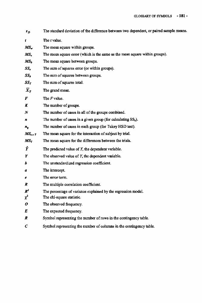
GLOSSARY OF SYMBOLS - 181 -
SD The standard deviation of the difference between two dependent, or paired sample means.
t The t value.
MSW The mean square within groups.
MSe The mean square error (which is the same as the mean square within groups).
MSb The mean square between groups.
SSe The sum of squares error (or within groups).
SSb The sum of squares between groups.
SST The sum of squares total.
XT The grand mean.
F The F value.
K The number of groups.
N The number of cases in all of the groups combined.
n The number of cases in a given group (for calculating SSb).
ng The number of cases in each group (for Tukey HSD test).
MSS x T The mean square for the interaction of subject by trial.
MST The mean square for the differences between the trials.A
Y The predicted value of 7, the dependent variable.
Y The observed value of Y, the dependent variable.
b The unstandardized regression coefficient.
a The intercept.
e The error term.
R The multiple correlation coefficient.
R2 The percentage of variance explained by the regression model.X2 The chi-square statistic.
O The observed frequency.
E The expected frequency.
R Symbol representing the number of rows in the contingency table.
C Symbol representing the number of columns in the contingency table.
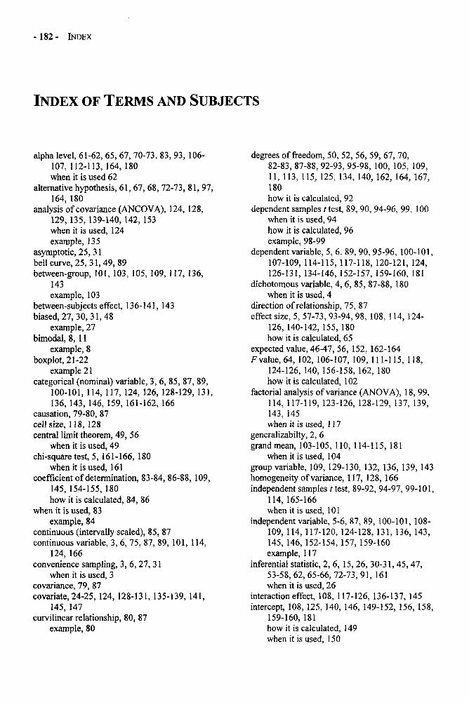
-182 - INDEX
INDEX OF TERMS AND SUBJECTS
alpha level, 61-62, 65, 67, 70-73, 83, 93, 106-107, 112-113, 164, 180when it is used 62
alternative hypothesis, 61, 67, 68, 72-73, 81, 97,164, 180
analysis of covariance (ANCOVA), 124, 128,129, 135, 139-140, 142, 153when it is used, 124example, 135
asymptotic, 25, 31bell curve, 25, 31, 49, 89between-group, 101, 103, 105, 109, 117, 136,
143example, 103
between-subjects effect, 136-141, 143biased, 27, 30, 31, 48
example, 27bimodal, 8, 11
example, 8boxplot, 21-22
example 21categorical (nominal) variable, 3, 6, 85, 87, 89,
100-101, 114, 117, 124, 126, 128-129, 131,136, 143, 146, 159, 161-162, 166
causation, 79-80, 87cell size, 118, 128central limit theorem, 49, 56
when it is used, 49chi-square test, 5, 161-166, 180
when it is used, 161coefficient of determination, 83-84, 86-88, 109,
145, 154-155, 180how it is calculated, 84, 86
when it is used, 83example, 84
continuous (intervally scaled), 85, 87continuous variable, 3, 6, 75, 87, 89, 101, 114,
124, 166convenience sampling, 3, 6, 27, 31
when it is used, 3covariance, 79, 87covariate, 24-25, 124, 128-131, 135-139, 141,
145, 147curvilinear relationship, 80, 87
example, 80
degrees of freedom, 50, 52, 56, 59, 67, 70,82-83, 87-88, 92-93, 95-98, 100, 105, 109,11, 113, 115, 125, 134, 140, 162, 164, 167,180how it is calculated, 92
dependent samples t test, 89, 90, 94-96, 99, 100when it is used, 94how it is calculated, 96example, 98-99
dependent variable, 5, 6. 89, 90, 95-96, 100-101,107-109, 114-115, 117-118, 120-121, 124,126-131, 134-146, 152-157, 159-160, 181
dichotomous variable, 4, 6, 85, 87-88, 180when it is used, 4
direction of relationship, 75, 87effect size, 5, 57-73, 93-94, 98, 108, 114, 124-
126, 140-142, 155, 180how it is calculated, 65
expected value, 46-47, 56, 152, 162-164F value, 64, 102, 106-107, 109, 111-115, 118,
124-126, 140, 156-158, 162, 180how it is calculated, 102
factorial analysis of variance (ANOVA), 18, 99,114, 117-119, 123-126, 128-129, 137, 139,143, 145when it is used, 117
generalizabilty, 2, 6grand mean, 103-105, 110, 114-115, 181
when it is used, 104group variable, 109, 129-130, 132, 136, 139, 143homogeneity of variance, 117, 128, 166independent samples nest, 89-92, 94-97, 99-101,
114, 165-166when it is used, 101
independent variable, 5-6, 87, 89, 100-101, 108-109, 114, 117-120, 124-128, 131, 136, 143,145, 146, 152-154, 157, 159-160example, 117
inferential statistic, 2, 6, 15, 26, 30-31, 45, 47,53-58, 62, 65-66, 72-73, 91, 161when it is used, 26
interaction effect, 108, 117-126, 136-137, 145intercept, 108, 125, 140, 146, 149-152, 156, 158,
159-160, 181how it is calculated, 149when it is used, 150
INDEX - 183 -
interquartile range (IQR), 13-14, 21-22example, 21
Kruskal-Wallis, 161, 166kurtosis, 27-28, 31leptokurtic, 28, 31main effect, 117-128, 136-137, 142mean, 1, 7-22, 25, 29-30, 33-49, 180
when it is used, 7how it is calculated, 8example, 9
mean square between, 102-103, 111, 114, 181how it is calculated, 106
mean square within (or error), 102, 114-115, 181how it is calculated, 106
median, 4, 7-11, 13, 21-23, 25, 31, 40, 124,180how it is calculated, 8example, 9
mode, 4, 7-11, 25, 31-32when it is used, 8example, 9
moderator, 117, 128multicollinearity, 155, 159multimodal, 8, 11multiple correlation coefficient, 155, 160, 180multiple regression, 87, 118, 145-146, 152-160,
179when it is used, 154example, 158
negative correlation, 75-76, 79, 87, 146example, 76
negatively skewed, 9-10, 19, 27-31example, 19
nonparametric, 5, 91, 161, 166normal distribution, 5, 9, 22, 25-31, 34-43, 49-
51, 59, 62, 89, 92, 97example, 25
null hypothesis, 26, 60-62, 68, 70-73, 81, 98-99,101, 164-165, 180example, 62
observed value, 106, 107, 150-151, 155, 159-160, 163-164, 181
one-way ANOVA, 99, 101-115, 117-118, 126,128, 132, 161, 165-166when it is used, 101
ordinary least squares regression (OLS), 148-149, 160
outliers, 10-11overpredicted, 152, 160paired t test, SEE DEPENDENT t TESTparameter, 1, 6-7, 11, 15, 47, 58-59, 61-62, 64,
66-67, 72, 75partial (controlled effects), 118, 128
product-moment correlation coefficient.,, 78, 87, 180
when it is used, 75how it is calculated, 78
perfect negative correlation, 76, 87perfect positive correlation, 76, 87phi coefficient, 75, 85, 88, 180platykurtic, 28-29, 31point-biserial coefficient, 75, 85, 88population, 1-3, 6-8, 11, 15-17, 22-23, 26-27, 30-
31, 34, 38-39, 44-53, 56-62, 64-65, 67-68,70-72, 74-75, 81, 83, 88-90, 92-95, 99, 101-102, 115, 180
positive correlation, 75-76, 80, 88, 146-147example, 75
positively skewed, 9-10, 27-28, 31example, 28
post-hoc test, 106-107, 109, 112-115, 123practical significance, 58, 65-66, 72-73, 125, 155predicted value, 146, 148-152, 155-156,
159-160, 181how it is how it is calculated, 146
priori, 61, 72, 107, 113-114probability, 26, 31, 43, 49-54, 58-61, 64, 66-67,
70-73, 82-83, 93, 97, 99, 101, 120, 163,165-166, 180example, 53
p value, 60, 62, 65, 67, 70, 72-73, 83, 86, 97,109, 120, 126, 140-141, 156-159, 180
random chance, 49, 59-60random sampling, 3-6, 27, 31, 62random sampling error, 54, 59, 61-62, 64, 73, 93raw scores, 33, 38-42, 44, 180
example, 41regression coefficient, 45, 59, 146, 149-150,
156-157, 158-160, 181regression equation, 146, 148-152, 156, 160
how it is calculated, 146, 152examples, 150, 156
regression line, 146, 148-152, 160example, 151
representative sampling, 3, 6, 27, 31example, 3
residuals, 151-152, 155, 160example, 152
sampling distribution of the mean, 46-49, 56, 58,62how it is calculated, 47example, 46
scatterplot, 147-149, 151, 160examples, 148, 151
shared variance, 84, 87-88, 114, 128, 154-155simple effects, 118, 123-124, 127-128
Pearson
75
- 184 - INDEX
simple linear regression, 145-146, 152, 159-16spearman rho coefficient, 75, 85, 88standard deviation, 11, 13-23, 29-30, 33-37, 41-
59, 65-67, 71-75, 78-79, 89, 91, 94-96, 99-101, 103, 108, 118, 139-140, 147, 149, 156,180-181how it is calculated, 16example, 18-21
standard error, 45-46, 59-65, 70-71, 73, 90-92,95, 112how it is calculated for the mean, 59example for the mean, 54
standard error of the difference between themeans, 91-95, 97, 99-100how it is calculated, 95
standard score, 33, 44, 56, 180standardization, 31, 33-34, 44, 157standardized regression coefficient, 146, 149,
156, 158, 160, 181statistical significance, 56-73, 81, 87, 93, 98-99,
101, 115, 117, 125, 156example, 68
strength, magnitude, 88studentized range statistic, 112-113, 115, 168sum of squared deviations, sum of squares, 15,
18, 23, 103, 106, 109, 148-149, 160, 180
sum of squares between, 103-104, 106, 109-110, 115how it is calculated, 104
sum of squares error, 103-104, 106, 109-110,115, 157, 180how it is calculated, 104
sum of squares total, 104-105, 115, 181symmetrical, 21, 25, 30-31, 34, 37, 41, 97theoretical distribution, 22 , 26, 32, 50, 56, 162time, trial, 143, 181truncated range, 80, 88TukeyHSD, 107, 109, 112-113, 115, 168, 181
how it is calculated, 107examples, 109, 112-113
type I error, 60-62, 73, 101underpredicted, 151, 160unique variance, 154, 155, 160variance, 7, 10, 13-23, 53, 79, 83-84, 87-88, 91,
97, 101, 103, 105, 108-109, 114-119, 124-125, 129-138, 143, 152-161, 179, 180how it is calculated, 16
within-group, 101-103, 115, 117, 128, 181within-subjects design, 135, 143z score, 31, 33-44, 64, 75, 78-79, 88-89,
157, 180how it is calculated, 34example, 41
z score, 31, 33-44, 49-51, 64, 75, 78-79, 88-89,
Related Documents


