172385052 solution-manual-operation-management-ch-17-pdf

247

17C H A P T E R

Maintenance and Reliability

DISCUSSION Q UESTIONS 1. The objective of maintenance and reliability is to maintain the capability of the system while controlling costs.

2. Candidates for preventive maintenance can be identified by looking at the distributions for MTBF (mean time between fail-ures). If the distributions have a small standard deviation, they are usually a candidate for preventive maintenance.

3. Infant mortality refers to the high rate of failures that exists for many products when they are relatively new.

4. Simulation is an appropriate technique with which to investi-gate maintenance problems because failures tend to occur ran-domly, and the probability of occurrence is often described by a probability distribution that is difficult to employ in a closed-form mathematical solution.

5. Training of operators to perform maintenance may improve morale and commitment of the individual to the job or organiza-tion. On the other hand, all operators are not capable of perform-ing the necessary maintenance functions or they may perform them less efficiently than a specialist. In addition, it is not always cost effective to purchase the necessary special equipment for the operator’s use.

6. Some ways in which the manager can evaluate the effective-ness of the maintenance function include:

Maintenance productivity as measured by: Units of production

Maintenance hours

or Maintenance hours

Replacement cost of investment

or Actual maintenance hours to do job

Standard maintenance hours to do job

Machine utilization as measured by: ( ) ( )

( )

A B C D

A B

− − +−

where: A = total available operating hours B = scheduled downtime C = scheduled mechanical downtime D = nonscheduled mechanical downtime

Effectiveness of preventive maintenance as measured by:

Emergency maintenance hours1

Preventive maintenance hours−

7. Machine design can ameliorate the maintenance problem by, among other actions, stressing component reliability, simplicity of design and the use of common or standard components, simplicity of operation, and provision of appropriate product explanations and user instructions.

8. Information technology can play a number of roles in the maintenance function, among them:

Files of parts and vendors Management of data regarding failures Active monitoring of system states Problem diagnosis and tracking Via simulation—pretesting and evaluation of mainte-

nance policy Enabling more precise control to reduce the likelihood of

failure Enabling improved system design

9. The best response would probably be to enumerate the actual costs, both tangible and intangible, for each practice.

Costs of waiting until it breaks to fix it might include:

Unnecessary damage to the machine Significant down time on the production line Random interruption of the production schedule Ruined raw materials Poor quality of products produced in a time period prior

to breakdown Frustration of employees Costs to repair the machine

Costs of preventive maintenance would include primarily the cost to replace the machine component. Downtime could be sched- uled so as to reduce its cost; and the frustration of employees, etc., would certainly be less than incurred when the breakdown occurs.

10. Only when preventive maintenance occurs prior to all outliers of the failure distribution will preventive maintenance preclude all failures. Even though most breakdowns of a component may occur after time t, some of them may occur earlier. The earlier breakdowns may not be eliminated by the preventive maintenance policy. A distribution of natural causes exists.

248 CHAPTER 17 M A I N T E N A N C E A N D R E L I A B I L I T Y

ETHICAL DILEM M A Yes, as the man said: “You can be perfectly safe and never get off the ground.” But the significant question for this ethical dilemma is: “Do we need to send men and women into space?” Given the sophistication evidenced in automation, simulation, Drones, the Mars Lander, etc., is staffed space travel necessary? And this is without considering the risk, which from a reliability perspective and in practice is huge and documented with the cost of many lives. Additionally, sending people into space drives the cost to astronomical levels (excuse the pun). There seems little doubt that men and women are put at risk for publicity, domestic politics, and geopolitical reasons. And people leave a lot of junk out there that creates other problems for unstaffed space travel and satel-lites, whose value has been documented. Should we keep sending people?

ACTIVE MO DEL EXERCISES

ACTIVE MODEL 17.1: Series Reliability 1. Would it be better to increase the worst clerk’s reliability from .8 to .81 or the best clerk’s reliability from .99 to 1?

The worst clerk’s reliability from .8 to .81

2. Is it possible to achieve 90% reliability by focusing on only one of the three clerks?

No—the best we can do is 89.1% reliability even with R2 to 100%.

ACTIVE MODEL 17.2: Redundancy 1. If one additional clerk were available, which would be the best place to add this clerk as back-up?

At R2, yielding a system reliability of 97.23%.

2. What is the minimum number of total clerks that need to be added as back-up in order to achieve a system reliability of 99%?

3 more clerks—one more at each process.

END-OF-CHAPTER PROBLEMS 17.1 Using Figure 17.2: n = 50. Average reliability of compo-nents = 0.99. Average reliability of system = .9950 = 0.62. Actual (calculated) reliability of the system = 0.605.

17.2 From Figure 17.2, about 13% overall reliability (or .995400)

17.3 E(breakdowns/year) = 0.1(0) + 0.1(1) + 0.25(2) + 0.2(3) + 0.25(4) + 0.1(5)

= 0.1 + 0.5 + 0.6 + 1.0 + 0.5 = 2.7 breakdowns

17.4 E(daily breakdowns) = 0.1(0) + 0.2(1) + 0.4(2) + 0.2(3) + 0.1(4)

= 0 + 0.2 + 0.8 + 0.6 + 0.4 = 2.0

Expected cost = 2($50) = $100 daily

17.5 Let R equal the reliability of the components. Then R1 × R2 × R3 = Rs, the reliability of the overall system. Therefore, R3 = 0.98 and each R ≅ 0.9933. Therefore, a reliability of approximately 99.33% is required of each component.

17.6 (a) Percent of failures [FR(%)]

( ) 5% 0.05 5.0%

100F = = =

(b) Number of failures per unit hour [(FR(N)]:

( ) Number of failures

Total time Nonoperating timeFR N =

−

where

Total time = (5,000 hrs) × (100 units) = 500,000 unit-hours

Nonoperating time = (2,500 hrs) × (5 units) = 12,500

5 5( )

500,000 12,500 487,500

0.00001026failure unit-hour

FR N = =−

=

(c) Number of failures per unit year:

Failure/unit-year = FR(N) × 24 hr/day × 365 days/yr = 0.00001026 × 24 × 365 = 0.08985

(d) Failures from 1100 installed units:

Failures/year = 1100 units × 0.08985 failures/unit-year = 98.83

17.7 (a) ( ) 4% 40%

10FR = =

(b)

(c) MTBF = 1 .000008247 121,256 hours=

17.8 The overall system has a reliability of 0.9941, or approxi-mately 99.4%.

Alternatively, 0.95 + (1 − 0.95) × 0.882 = 0.95 + 0.0441 = 0.9941

{}

[ ]

FR N ⎡= × − × + ×⎣⎤+ × ⎦

− =

( ) 4 (10 60,000) (50,000 1) (35,000 1)

(15,000 2)

4 600,000 115,000 4 485,000

.000008247 failures per unit hour

set

CHAPTER 17 M A I N T E N A N C E A N D R E L I A B I L I T Y 249

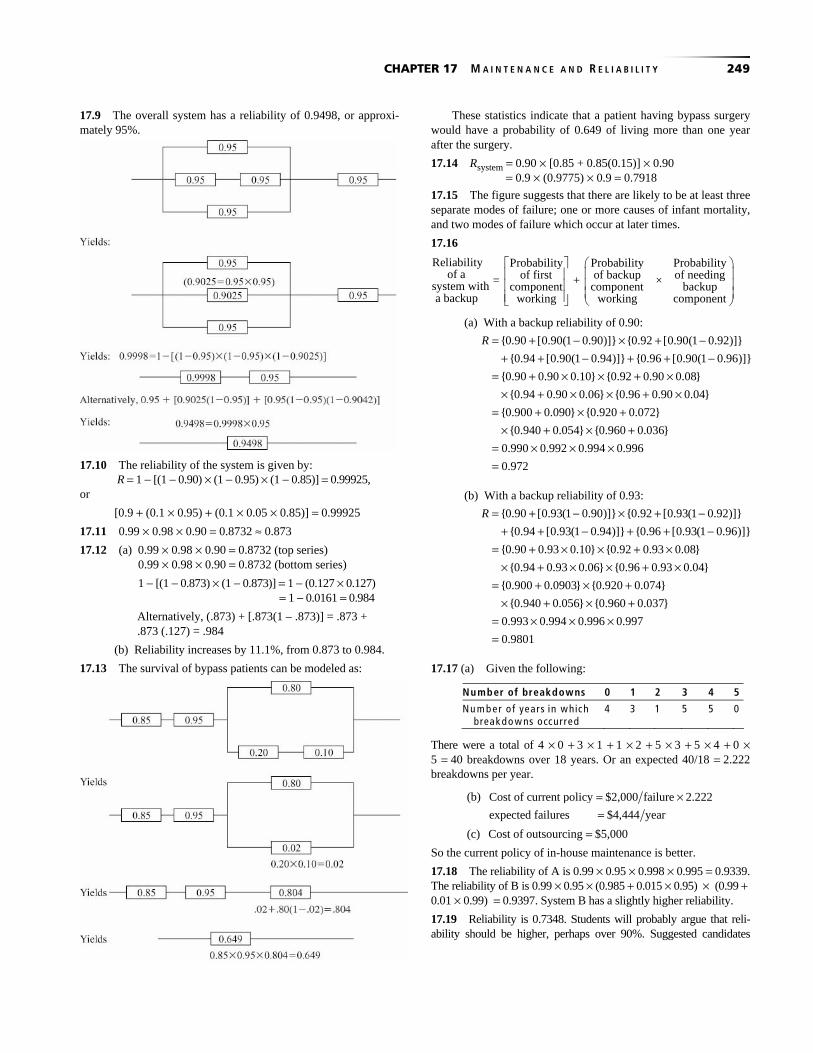
17.9 The overall system has a reliability of 0.9498, or approxi-mately 95%.

17.10 The reliability of the system is given by: R = 1 − [(1 − 0.90) × (1 − 0.95) × (1 − 0.85)] = 0.99925,

or

[0.9 + (0.1 × 0.95) + (0.1 × 0.05 × 0.85)] = 0.99925

17.11 0.99 × 0.98 × 0.90 = 0.8732 ≈ 0.873

17.12 (a) 0.99 × 0.98 × 0.90 = 0.8732 (top series) 0.99 × 0.98 × 0.90 = 0.8732 (bottom series)

1 − [(1 − 0.873) × (1 − 0.873)] = 1 − (0.127 × 0.127) = 1 − 0.0161 = 0.984

Alternatively, (.873) + [.873(1 – .873)] = .873 + .873 (.127) = .984

(b) Reliability increases by 11.1%, from 0.873 to 0.984.

17.13 The survival of bypass patients can be modeled as:

These statistics indicate that a patient having bypass surgery would have a probability of 0.649 of living more than one year after the surgery.

17.14 Rsystem = 0.90 × [0.85 + 0.85(0.15)] × 0.90 = 0.9 × (0.9775) × 0.9 = 0.7918

17.15 The figure suggests that there are likely to be at least three separate modes of failure; one or more causes of infant mortality, and two modes of failure which occur at later times.

17.16

(a) With a backup reliability of 0.90:

{0.90 [0.90(1 0.90)]} {0.92 [0.90(1 0.92)]}

{0.94 [0.90(1 0.94)]} {0.96 [0.90(1 0.96)]}

{0.90 0.90 0.10} {0.92 0.90 0.08}

{0.94 0.90 0.06} {0.96 0.90 0.04}

{0.900 0.090} {0.920 0.072}

{0.940 0.054}

R = + − × + −+ + − + + −

= + × × + ×× + × × + ×

= + × +× + ×{0.960 0.036}

0.990 0.992 0.994 0.996

0.972

+= × × ×=

(b) With a backup reliability of 0.93:

{0.90 [0.93(1 0.90)]} {0.92 [0.93(1 0.92)]}

{0.94 [0.93(1 0.94)]} {0.96 [0.93(1 0.96)]}

{0.90 0.93 0.10} {0.92 0.93 0.08}

{0.94 0.93 0.06} {0.96 0.93 0.04}

{0.900 0.0903} {0.920 0.074}

{0.940 0.056}

R = + − × + −+ + − + + −

= + × × + ×× + × × + ×

= + × +× + {0.960 0.037}

0.993 0.994 0.996 0.997

0.9801

× += × × ×=

17.17 (a) Given the following:

Number of breakdowns 0 1 2 3 4 5

Nu m b er o f years in which breakd o w ns occurred

4 3 1 5 5 0

There were a total of 4 × 0 + 3 × 1 + 1 × 2 + 5 × 3 + 5 × 4 + 0 × 5 = 40 breakdowns over 18 years. Or an expected 40/18 = 2.222 breakdowns per year.

(b)

(c) Cost of outsourcing $5,000=

So the current policy of in-house maintenance is better.

17.18 The reliability of A is 0.99 × 0.95 × 0.998 × 0.995 = 0.9339. The reliability of B is 0.99 × 0.95 × (0.985 + 0.015 × 0.95) × (0.99 + 0.01 × 0.99) = 0.9397. System B has a slightly higher reliability.

17.19 Reliability is 0.7348. Students will probably argue that reli-ability should be higher, perhaps over 90%. Suggested candidates

Cost of current policy $2,000 failure 2.222

expected failures $4,444 year

= ×=

Reliability Probability Probability Probability of a of first of backup of needing = + × system with component component backupa backup working working component

⎡ ⎤ ⎛ ⎞⎜ ⎟⎢ ⎥⎜ ⎟⎢ ⎥⎜ ⎟⎢ ⎥⎣ ⎦ ⎝ ⎠

250 CHAPTER 17 M A I N T E N A N C E A N D R E L I A B I L I T Y

for backup include fuller inventory, more cashier lanes and over-rides for faulty scanning. Suggested candidates for redesign in-clude bagging and exit.

AD DITIONAL HO ME W O RK PROBLEMS Here are solutions to additional homework problems at www.myomlab.com.

17.20 From Figure 17.2, about 82% overall reliability (or .9810)

17.21 Expected number of breakdowns =

0 × 0.3 = 0.0 1 × 0.2 = 0.2 2 × 0.2 = 0.4 3 × 0.3 = 0.9

1.5

at a cost of $10 each equals $15

17.22 The reliability of the system is given by: R = 0.90 × 0.95 × 0.80 × 0.85 = 0.58

17.23 (a) Percent of failures [FR(%)]:

( ) = = =4% 0.02 2.0%

200FR

(b) Number of failures per unit-hour [(FR(N)]:

( ) Number of failures

Total time nonoperating timeFR N =

−

where: Total time (4,000 hr.) (200 units)

800,000 unit-hours

Non-operating time (2,000 hr.) (4 units)

8,000

= ×== ×=

( ) 4 4

800,000 8,000 792,000

0.00000505 failures unit-hour

FR N = =−

=

(c) Number of failures per unit year:

Failure unit-year ( ) 24 hr day

365 days yr

0.00000505 24 365 0.044

FR N= ××

= × × =

(d) Failures from 500 installed units:

Failures year 500 units 0.044 failures unit-year

22.1

= ×=

17.24 First, find the cost of the breakdowns without the mainte-nance contract. The expected number of breakdowns per week without the maintenance contract is found by:

( ) ( )

1[(1 0) (1 1) (3 2) (5 3) (9 4)

50(11 5) (7 6) (8 7) (5 8)]

1[0 1 6 15 36 55 42 56 40]

50251

5.0250

i iE B n p n= ∑ ×

= × + × + × + × + ×

+ × + × + × + ×

= + + + + + + + +

= =

Therefore, with no maintenance contract, the company ex-periences an average of 5.02 breakdowns per week. The cost of breakdowns when no maintenance contract is held is given by:

5.02breakdowns week $250 breakdown

$1255 week

C = ×=

Second, find the cost with the maintenance contract. We are told that an average of three breakdowns per week occurs with the maintenance contract. The cost of break-downs when the maintenance contract is held is given by:

= + ×=

$645 week 3 breakdowns week $250 breakdown

$1395 week

C

Comparing the costs, we find that eliminating the mainte-nance contract would save approximate $140/week ($1395 −$1255).

VIDEO CASE STUDY

MAINTENANCE DRIVES PROFITS AT FRITO-LAY 1. What might be done to help take Frito-Lay to the next level of outstanding maintenance? Consider factors such as sophisticated software.

Frito-Lay’s Florida plant is establishing a world-class benchmark, with 1½% unscheduled downtime. Total un-scheduled downtime is 2½%, but 1% of that is used for pro-duction changeovers. With each 1% of downtime having a negative profit impact of $200,000, keeping the plant oper-ating is very significant. This is facilitated by a two-section board that has operations issues on one side and mainte-nance issues on the other side. The manager’s job is to call on maintenance to make the correction and provide an ex-plicit description of the problem. Maintenance software, as described in the text, may provide the next step of informa-tion and control for Frito-Lay’s facility maintenance per-sonnel.

2. What are the advantages and disadvantages of giving more responsibility for machine maintenance to the operator?

Advantages of more responsibility given for maintenance to machine operators are empowerment, the advantages of job enrichment and good job design, and faster response time (more “up” time for the equipment). Frito-Lay provides a case study of machine operators taking advantage of empowerment. Disadvantages are increased training budgets, a modest in-crease for the necessary tools and testing equipment, and a need to motivate operators (some of whom may not be in-terested in obtaining additional skills).

3. Discuss the pros and cons of hiring multi-craft maintenance personnel.

Multi-craft maintenance personnel are paid more; they tend to be expensive. But when trying to cover 24/7 shifts, using multi-craft personnel may be much cheaper than having several people on staff around the clock. Multi-craft person-nel also increase the training budget.

CHAPTER 17 M A I N T E N A N C E A N D R E L I A B I L I T Y 251

1

2ADDITIONAL CASE STUDIES*

WORLDWIDE CHEMICAL COMPANY

An excellent case for introducing the management and duties of a maintenance department.

1. Smith and Henson are exhibiting very poor leadership. They can and should develop a maintenance plan. Maintenance and reliability are key factors in manufacturing productivity and must be treated as such.

2. The alternative to the current fire-fighting approach is devel-opment of a realistic preventive and scheduled maintenance plan with the appropriate level of staffing. Scheduled mainte-nance is maintenance that involves overhauls and major modifications. Maintenance work is handled just like other work, with schedules, due dates, work orders, accurate bills of material, proper skills and tools available, etc. Emergency maintenance should be a small part of all maintenance (say 5%) in well-managed facilities.

3. When scheduled maintenance is to occur, production schedul-ing personnel build that downtime into the production sched-ule. This may mean that certain machines are down during the day and or that maintenance is done on off shifts, weekends, or vacation periods.

4. Maintenance mechanics perform only preventive maintenance that cannot be performed by empowered operators. Mainte-nance departments are staffed to meet the preventive mainte-nance requirements that require a higher level of skills. Addi-tionally, maintenance departments are staffed to perform equipment/process improvements and scheduled work, plus an allowance for emergency work. A reasonable breakdown is:

5% for emergency maintenance 25% for equipment/process improvements 70% for preventive and scheduled maintenance on a regular

schedule

5. Good records of machine/equipment performance will allow operations managers to determine the mean time between failure (MTBF): Additionally, predictive maintenance (vibra-tion analysis, oil analysis, thermography, pressure differential measurement, trend analysis [SPC], product output quality, and equipment performance [such as cumulative operating hours and downtime by machine]) allows management to predict equipment failures.

CARTAK’S DEPARTMENT STORE

This reliability case study does not really require a computer, but it does require some thought. In order for the checking system to fail, the item must be both miscoded and misverified. This means that coding and verification act as parallel (not serial) process. There are two items in parallel and a total reliability of 0.99768. Students must add to that a third item (second verifier) with a reliability of 0.92. This yields an overall reliability of 0.99981 [= 0.99768 + 0.92 (1 – 0.99768)]. The net benefit is that reliability will increase by 0.99981 – 0.99768 = 0.00213. In other words, 21 out of 10,000 additional items will be caught by adding the new verifier. It probably is not worth the cost of adding a new verifier, although it may be if the errors themselves are large enough.

In a related vein, if the error is an overcharge, customers might notice and become upset. Many stores do not require cus-tomers to pay for items for which they have been overcharged; in effect, the stores use their customers as verifiers. It would also make sense for stores to tell customers that they will not be charged for items for which they have been undercharged.

* These case studies are found at our Web sites, www.pearsonhighered.com/heizer and www.myomlab.com.