17-link-ma-aloha - zoo.cs.yale.eduzoo.cs.yale.edu/classes/cs434/cs434-2012-fall/lectures/17-link-ma... · – e.g., Location Manager, ... WCDMA downlink 33 Summary Outline ... (BTS)

Page 1

Link Layer: Partitioning Dimensions;

Media Access Control using Aloha

Y. Richard Yang

11/01/2012

2

Outline

❒ Admin. and recap ❒  Intro to link layer ❒ Media access control

❍ ALOHA protocol

Admin. ❒ Assignment 3

❍ Due date: coming Monday ❍ Check web site for office hours and FAQs

❒  Project proposal (due Friday) ❍  Please send email to [email protected] by

end of day ❍ Subject: Project Proposal ❍ Content:

•  Team members: •  Topic: •  One paragraph rough idea:

❒  Exam: next Tuesday in class 3 4

Recap

❒ App layer ❍ Handles issues such as UI ❍ Uses lower-layer provided abstractions, e.g.,

•  network abstraction –  e.g., HttpURLConnection in GoogleSearch Example

•  location service abstraction –  e.g., Location Manager, and Location Listener in

Assignment 3

❒  Physical layer capability ❍  sender sends a seq. of bits to a receiver

App Layer: Logical Communications

5

E.g.: application ❒  provide services

to users

❒  application protocol: ❍  send messages

to peer

6

Physical Communication application transport network

link physical

application transport network

link physical

application transport network

link physical

application transport network

link physical

network link

physical

data

data

Page 2

7

Protocol Layering and Meta Data Each layer takes data from above ❒  adds header (meta) information to create new data unit ❒  passes new data unit to layer below

8

Link layer: Context ❒  Data-link layer has

responsibility of transferring datagram from one node to another node

❒  Datagram may be transferred by different link protocols over different links, e.g., ❍  Ethernet on first link, ❍  frame relay on

intermediate links ❍  802.11 on last link

transportation analogy ❒  trip from New Haven to

San Francisco ❍  taxi: home to union

station ❍  train: union station to

JFK ❍  plane: JFK to San

Francisco airport ❍  shuttle: airport to

hotel

9

Main Link Layer Services q  Framing

o  encapsulate datagram into frame, adding header, trailer and error detection/correction

q  Multiplexing/demultiplexing o  use frame headers to identify src, hop dest

q  Media access control q  Reliable delivery between adjacent nodes

o  seldom used on low bit error link (fiber, some twisted pair) o  common for wireless links: high error rates

10

Link Adaptors

❒  link layer typically implemented in “adaptor” (aka NIC) ❍  Ethernet card,

modem, 802.11 card ❒  adapter is semi-

autonomous, implementing link & physical layers

❒  sending side: ❍  encapsulates datagram in

a frame ❍  adds error checking bits,

rdt, flow control, etc. ❒  receiving side

❍  looks for errors, rdt, flow control, etc

❍  extracts datagram, passes to receiving node

sending node

frame

receiving node

datagram

frame

adapter adapter

link layer protocol

11

Outline

❒  Recap ❒  Introduction to link layer ❒ Wireless link access control

12

Wireless Access Problem

❒ Single shared broadcast channel ❍ thus, if two or more simultaneous

transmissions by nodes, due to interference, only one node can send successfully at a time

Page 3

13

Wireless Access Problem

❒  The general case is challenging and largely still open

❒  We start with the simplest scenario (e.g., 802.11 or cellular up links) in this class: ❍  a single receiver (the Access Point)

14

Multiple Access Control Protocol

❒  Protocol that determines how nodes share channel, i.e., determines when nodes can transmit

❒  Communication about channel sharing must use channel itself !

❒  Discussion: properties of an ideal multiple access protocol.

15

Ideal Mulitple Access Protocol q  Efficient

q  Fair/rate allocation

q  Simple

16

MAC Protocols: a Taxonomy Goals ❒  efficient, fair, simple Three broad classes: ❒  channel partitioning

❍  divide channel into smaller “pieces” (time slot, frequency, code)

❒  non-partitioning ❍  random access

•  allow collisions ❍  “taking-turns”

•  a token coordinates shared access to avoid collisions

17

Outline

❒  Recap ❒  Introduction to link layer ❒ Wireless link access control

❍  partitioning dimensions

18

FDMA

FDMA: frequency division multiple access ❒  Channel divided into frequency bands ❒  A transmission uses a frequency band

freq

uenc

y ba

nds

time

5

1

4 3 2

6

Page 4

19

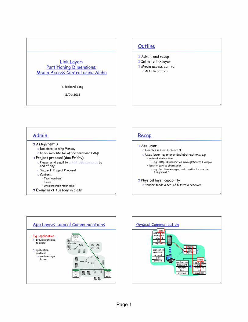
TDMA

TDMA: time division multiple access ❒  Time divides into frames; frame divides into slots ❒  A transmission uses a slot in a frame

20

Example: GSM

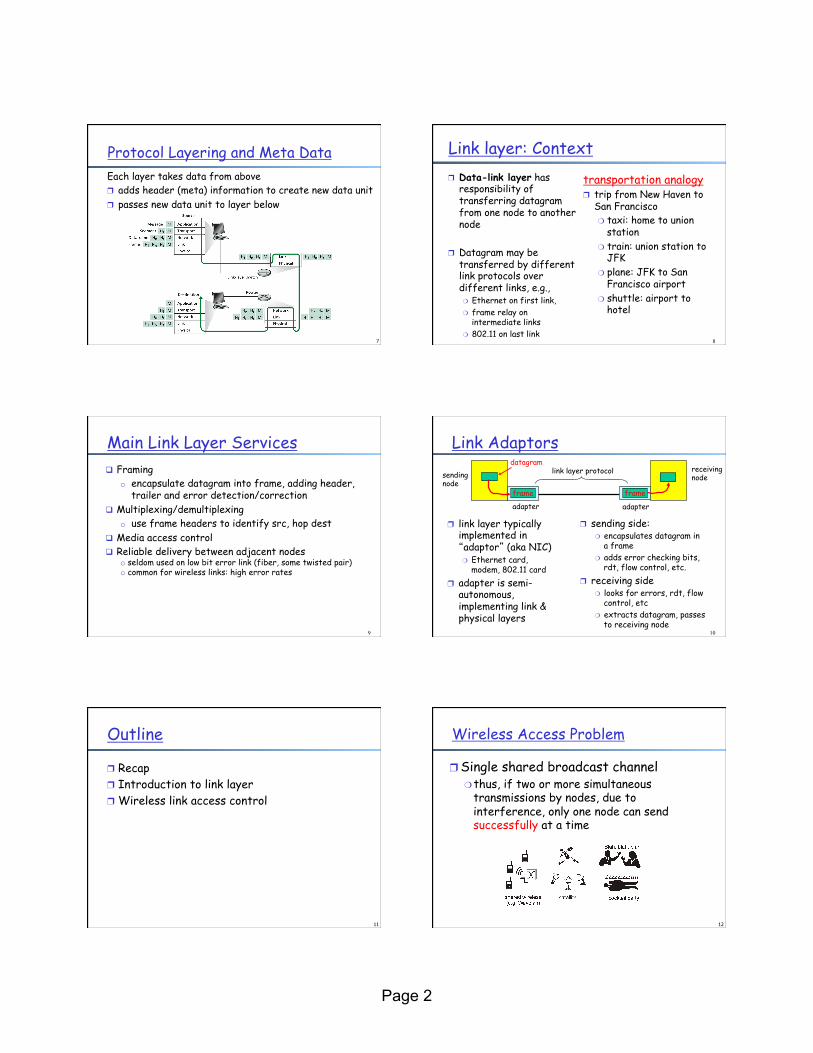
❒  A GSM operator uses TDMA and FDMA to divide its allocated frequency ❍  divide allocated spectrum into different physical

channels; each physical channel has a frequency band of 200 kHz

❍  partition the time of each physical channel into frames; each frame has a duration of 4.615 ms

❍  divides each frame into 8 time slots (also called a burst) ❍  each slot is a logical channel ❍  user data is transmitted through a logical channel

21

higher GSM frame structures

935-960 MHz 124 channels (200 kHz) downlink

890-915 MHz 124 channels (200 kHz) uplink

frequ

ency

time

1 2 3 4 5 6 7 8

GSM TDMA frame

4.615 ms

GSM - TDMA/FDMA

GSM time-slot (normal burst)

546.5 µs 577 µs

tail user data Training S guard space S user data tail

guard space

3 bits 57 bits 26 bits 57 bits 1 1 3

S: indicates data or control 22

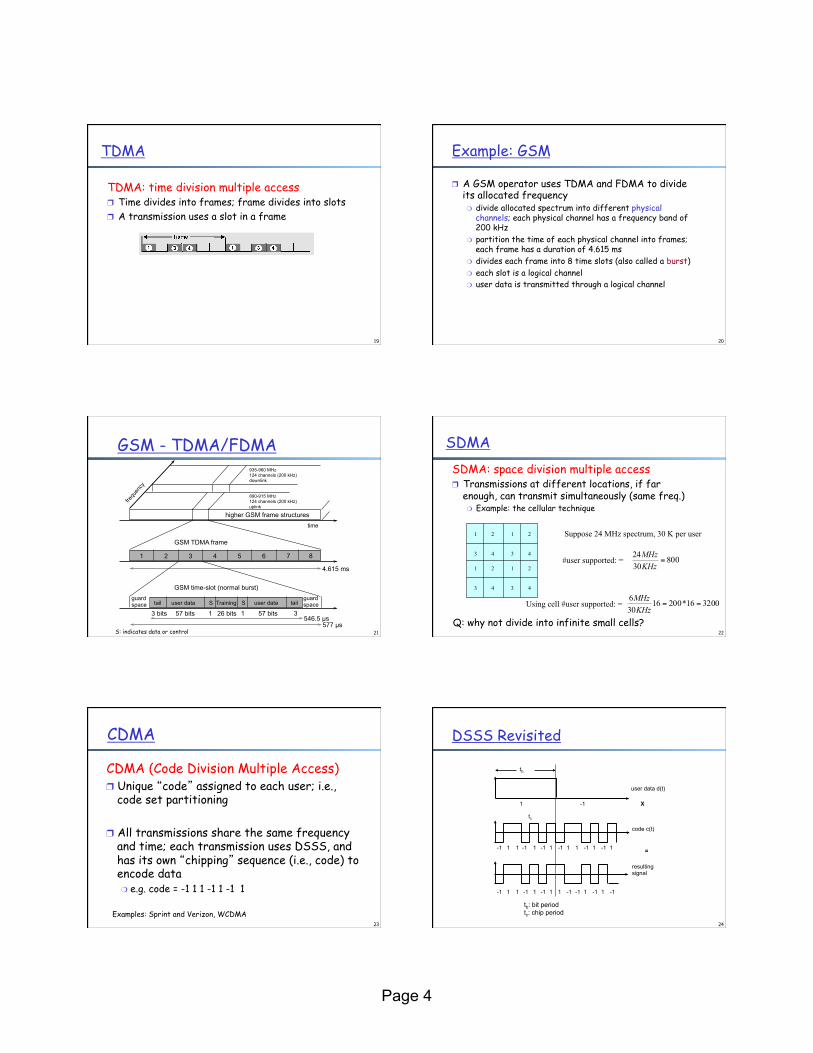
SDMA SDMA: space division multiple access ❒  Transmissions at different locations, if far

enough, can transmit simultaneously (same freq.) ❍  Example: the cellular technique

Suppose 24 MHz spectrum, 30 K per user

#user supported: = 8003024

=KHzMHz

1 2

3 4

1 2

3 4

1 2

3 4

1 2

3 4

Using cell #user supported: = 320016*20016306

==KHzMHz

Q: why not divide into infinite small cells?

23

CDMA

CDMA (Code Division Multiple Access) ❒ Unique “code” assigned to each user; i.e.,

code set partitioning

❒ All transmissions share the same frequency and time; each transmission uses DSSS, and has its own “chipping” sequence (i.e., code) to encode data ❍  e.g. code = -1 1 1 -1 1 -1 1

Examples: Sprint and Verizon, WCDMA 24

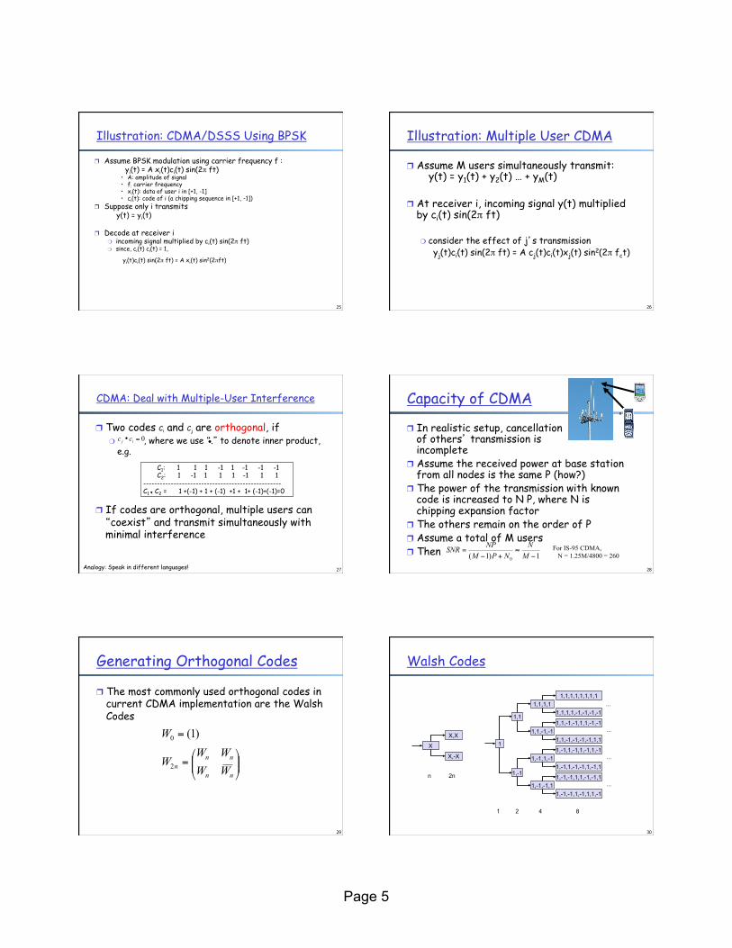
DSSS Revisited

user data d(t)

code c(t)

resulting signal

1 -1

-1 1 1 -1 1 -1 1 -1 1 -1 -1 1 1 1

X

=

tb

tc

tb: bit period tc: chip period

-1 1 1 -1 -1 1 -1 1 1 -1 1 -1 -1 1

Page 5

25

Illustration: CDMA/DSSS Using BPSK

❒  Assume BPSK modulation using carrier frequency f : yi(t) = A xi(t)ci(t) sin(2π ft)

•  A: amplitude of signal •  f: carrier frequency •  xi(t): data of user i in [+1, -1] •  ci(t): code of i (a chipping sequence in [+1, -1])

❒  Suppose only i transmits y(t) = yi(t)

❒  Decode at receiver i ❍  incoming signal multiplied by ci(t) sin(2π ft) ❍  since, ci(t) ci(t) = 1,

yi(t)ci(t) sin(2π ft) = A xi(t) sin2(2πft)

26

Illustration: Multiple User CDMA

❒ Assume M users simultaneously transmit: y(t) = y1(t) + y2(t) … + yM(t)

❒ At receiver i, incoming signal y(t) multiplied by ci(t) sin(2π ft)

❍  consider the effect of j’s transmission yj(t)ci(t) sin(2π ft) = A cj(t)ci(t)xj(t) sin2(2π fct)

27

CDMA: Deal with Multiple-User Interference

❒ Two codes Ci and Cj are orthogonal, if ❍  , where we use “.” to denote inner product,

e.g.

❒  If codes are orthogonal, multiple users can “coexist” and transmit simultaneously with minimal interference

•0=• ij cc

C1: 1 1 1 -1 1 -1 -1 -1 C2: 1 -1 1 1 1 -1 1 1 -------------------------------------------------- C1 . C2 = 1 +(-1) + 1 + (-1) +1 + 1+ (-1)+(-1)=0 •

Analogy: Speak in different languages! 28

Capacity of CDMA

❒  In realistic setup, cancellation of others’ transmission is incomplete

❒ Assume the received power at base station from all nodes is the same P (how?)

❒ The power of the transmission with known code is increased to N P, where N is chipping expansion factor

❒ The others remain on the order of P ❒ Assume a total of M users ❒ Then 1)1( 0 −

≈+−

=MN

NPMNPSNR For IS-95 CDMA,

N = 1.25M/4800 = 260

B

29

Generating Orthogonal Codes

❒ The most commonly used orthogonal codes in current CDMA implementation are the Walsh Codes

⎟⎟⎠

⎞⎜⎜⎝

⎛=

=

nn

nnn WW

WWW

W

2

0 )1(

30

Walsh Codes

1

1,1

1,-1

1,1,1,1

1,1,-1,-1

X

X,X

X,-X 1,-1,1,-1

1,-1,-1,1 1,-1,-1,1,1,-1,-1,1

1,-1,-1,1,-1,1,1,-1

1,-1,1,-1,1,-1,1,-1

1,-1,1,-1,-1,1,-1,1

1,1,-1,-1,1,1,-1,-1

1,1,-1,-1,-1,-1,1,1

1,1,1,1,1,1,1,1

1,1,1,1,-1,-1,-1,-1

1 2 4 8

n 2n

...

...

...

...

Page 6

31

Orthogonal Variable Spreading Factor (OSVF) ❒  Variable codes: Different users use different

lengths spreading codes ❒  Orthogonal: diff. users’ codes

are orthogonal

1

1,1

1,-1

1,1,1,1

1,1,-1,-1

X

X,X

X,-X 1,-1,1,-1

1,-1,-1,1 1,-1,-1,1,1,-1,-1,1

1,-1,-1,1,-1,1,1,-1

1,-1,1,-1,1,-1,1,-1

1,-1,1,-1,-1,1,-1,1

1,1,-1,-1,1,1,-1,-1

1,1,-1,-1,-1,-1,1,1

1,1,1,1,1,1,1,1

1,1,1,1,-1,-1,-1,-1

SF=1 SF=2 SF=4 SF=8

SF=n SF=2n

...

...

...

...

If user 1 is given code [1,1], what orthogonal codes can we give to other users?

32

WCDMA Orthognal Variable Spreading Factor (OSVF) ❒  Flexible code (spreading factor) allocation

❍  up link SF: 4 – 256 ❍  down link SF: 4 - 512

WCDMA downlink

33

Summary

❒ SDMA, TDMA, FDMA and CDMA are basic media partitioning techniques ❍  divide media into smaller “pieces” (space, time

slots, frequencies, codes) for multiple transmissions to share

❒ A remaining question is: how does a network allocate space/time/freq/code?

34

Outline

❒  Recap ❒  Introduction to link layer ❒ Wireless link access control

❍  partitioning dimensions ❍ media access protocols

35

GSM Logical Channels and Request

❒  Control channels ❍  Broadcast control channel

(BCCH) •  from base station, announces

cell identifier, synchronization ❍  Common control channels

(CCCH) •  paging channel (PCH): base

transceiver station (BTS) pages a mobile host (MS)

•  random access channel (RACH): MSs for initial access, slotted Aloha

•  access grant channel (AGCH): BTS informs an MS its allocation

❍  Dedicated control channels •  standalone dedicated control channel

(SDCCH): signaling and short message between MS and an MS

❒  Traffic channels (TCH)

❒  call setup from an MS BTS MS

RACH (request signaling channel)

AGCH (assign signaling channel)

SDCCH (request call setup)

SDCCH (assign TCH)

SDCCH message exchange

Communication

36

Slotted Aloha [Norm Abramson]

❒  Time is divided into equal size slots (= pkt trans. time)

❒  Node with new arriving pkt: transmit at beginning of next slot

❒  If collision: retransmit pkt in future slots with probability p, until successful.

Success (S), Collision (C), Empty (E) slots

A

B

Page 7

37

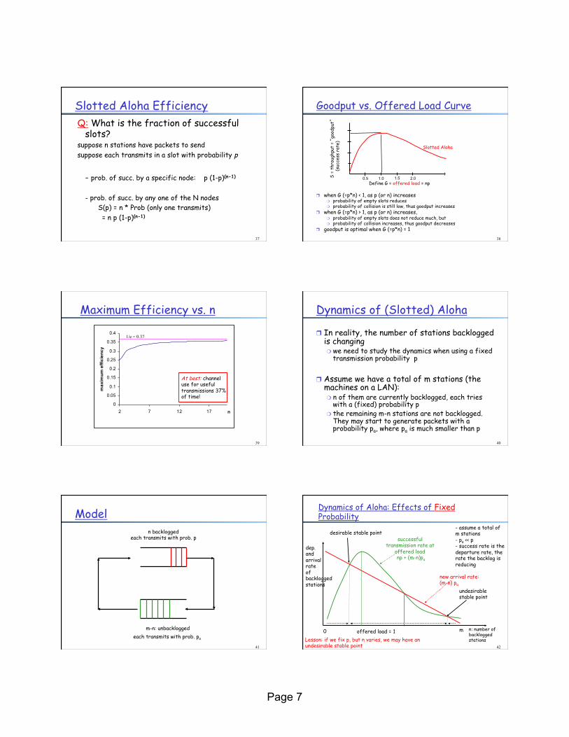
Slotted Aloha Efficiency Q: What is the fraction of successful

slots? suppose n stations have packets to send suppose each transmits in a slot with probability p

- prob. of succ. by a specific node: p (1-p)(n-1)

- prob. of succ. by any one of the N nodes S(p) = n * Prob (only one transmits)

= n p (1-p)(n-1)

38

Goodput vs. Offered Load Curve

S =

thro

ughp

ut =

“go

odpu

t”

(

succ

ess

rate

)

Define G = offered load = np 0.5 1.0 1.5 2.0

Slotted Aloha

❒  when G (=p*n) < 1, as p (or n) increases ❍  probability of empty slots reduces ❍  probability of collision is still low, thus goodput increases

❒  when G (=p*n) > 1, as p (or n) increases, ❍  probability of empty slots does not reduce much, but ❍  probability of collision increases, thus goodput decreases

❒  goodput is optimal when G (=p*n) = 1

39

Maximum Efficiency vs. n

0

0.05

0.1

0.15

0.2

0.25

0.3

0.35

0.4

2 7 12 17 n

max

imum

effi

cien

cy

1/e = 0.37

At best: channel use for useful transmissions 37% of time!

40

Dynamics of (Slotted) Aloha

❒  In reality, the number of stations backlogged is changing ❍ we need to study the dynamics when using a fixed

transmission probability p

❒ Assume we have a total of m stations (the machines on a LAN): ❍  n of them are currently backlogged, each tries

with a (fixed) probability p ❍  the remaining m-n stations are not backlogged.

They may start to generate packets with a probability pa, where pa is much smaller than p

41

Model n backlogged

each transmits with prob. p

m-n: unbacklogged each transmits with prob. pa

42

Dynamics of Aloha: Effects of Fixed Probability

n: number of backlogged stations

0 m

successful transmission rate at

offered load np + (m-n)pa

new arrival rate: (m-n) pa

desirable stable point

undesirable stable point

Lesson: if we fix p, but n varies, we may have an undesirable stable point

offered load = 1

- assume a total of m stations -  pa << p -  success rate is the departure rate, the rate the backlog is reducing

dep. and arrival rate of backlogged stations

Page 8

Backup Slides: Error Corrections Codes

43 44

Reed-Solomon Codes

❒  Very commonly used, send n symbols for k data symbols ❍  e.g., n = 255, k = 223

❒  We will discuss the original version (1960) ❍  modern versions are slightly different; they use generator

polynomial, but the idea is essentially the same

❒  If the data we want to send is (x0, x1,…, xk-1), where xi are data symbols, define polynomial P(t) = x0 + x1t + x2t + …xk-1tk-1

❒  Assume β is a generator of the symbol field (i.e., βi not equal to βj if i not equal to j)

❒  Then for the data sequence, send P(0), P(β), P(β2), P(βn-1) to receiver

45

Reed-Solomon Codes

❒  Receive the message P(0), P(β), P(β2), P(βn-1) ❒  If no error, can recover data from any k

equations:

)1)(1(1

2)1(2

110

1

)1(21

42

210

2

11

2210

0

...)(...

...)(

...)(

)0(

−−−

−−−

−−

−−

++++=

++++=

++++=

=

knk

nnn

kk

kk

xxxxP

xxxxPxxxxP

xP

ββββ

ββββ

ββββ

since any k equations are independent, they have a unique solution 46

Reed-Solomon Codes: Handling Errors

❒  But, what if s errors occur during transmission?

❒  Keep a counter (vote) for each solution

❒  Enumerate all combinations of k equations, for each combination, solve it, and increase the counter of the solution

❒  Identify the solution which gets the largest # of “votes”

47

Reed-Solomon Codes

❒ The transmitted data is the correct solution for n-s equations, and thus gets

votes (i.e., combinations of k equations) ❒ An incorrect solution can satisfy at most

k-1+s equations, and the # of votes it can get is at most:

⎟⎟⎠

⎞⎜⎜⎝

⎛ −

ksn

⎟⎟⎠

⎞⎜⎜⎝

⎛ +−

ksk 1

48

Reed-Solomon Codes

❒  If

or (n-s > k – 1 + s) or (n-k > 2s – 1) or (n-k ≥ s), it can correct any s errors

⎟⎟⎠

⎞⎜⎜⎝

⎛ +−>⎟⎟

⎠

⎞⎜⎜⎝

⎛ −

ksk

ksn 1

Page 9

49

Reed-Solomon Codes ❒  The voting-based decoding algorithm proposed in 1960 is

inefficient ❒  1967 - Berlekamp introduced first truly efficient algorithm

for both binary and nonbinary codes. Complexity increases linearly with number of errors

❒  1975 - Sugiyama, et al. Showed that Euclid’s algorithm can be used to decode R-S codes

❒  Below is a typical current decoder

50

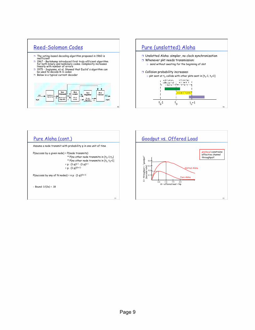
Pure (unslotted) Aloha ❒  Unslotted Aloha: simpler, no clock synchronization ❒  Whenever pkt needs transmission:

❍  send without awaiting for the beginning of slot

❒  Collision probability increases: ❍  pkt sent at t0 collide with other pkts sent in [t0-1, t0+1]

51

Pure Aloha (cont.) Assume a node transmit with probability p in one unit of time P(success by a given node) = P(node transmits) * P(no other node transmits in [t0-1,t0] * P(no other node transmits in [t0, t0+1] = p . (1-p)n-1 . (1-p)n-1

= p . (1-p)2(n-1)

P(success by any of N nodes) = n p . (1-p)2(n-1)

- Bound: 1/(2e) = .18

52

Goodput vs. Offered Load

S =

thro

ughp

ut =

“go

odpu

t”

(

succ

ess

rate

)

G = offered load = Np 0.5 1.0 1.5 2.0

0.1

0.2

0.3

0.4

Pure Aloha

protocol constrains effective channel throughput!

Slotted Aloha