Lesson 17 – Inventory Management Copyright – Harland E. Hodges, Ph.D 17-1 17 - 1 an inventory is a stock or store of goods and inventory management focuses on the planning and control of finished goods, raw materials, purchased parts work-in-progress and retail items Lesson 17 Inventory Management 17 - 2 Independent Demand A B(4) C(2) D(2) E(1) D(3) F(2) Dependent Demand Independent demand is uncertain Dependent demand is certain 17 - 3 Inventory must be managed at various locations in the production process. . Raw materials or purchased parts . Partially completed goods, called “work-in-progress (WIP)” . Finished goods inventories (manufacturing organizations) . Merchandise (retail organizations) . Replacement parts, tools and supplies . Goods-in-transit between locations (either plants, warehouses, or customers) Different Types Of Inventory

Welcome message from author
This document is posted to help you gain knowledge. Please leave a comment to let me know what you think about it! Share it to your friends and learn new things together.
Transcript

Lesson 17 – Inventory Management
Copyright – Harland E. Hodges, Ph.D 17-1
17 - 1
an inventory is a stock or store of goods and inventory management focuses on the planning and control of finished goods, raw materials, purchased parts work-in-progress and retail items
Lesson 17Inventory Management
17 - 2
Independent Demand
A
B(4) C(2)
D(2) E(1) D(3) F(2)
Dependent Demand
Independent demand is uncertainDependent demand is certain
17 - 3
Inventory must be managed at various locations in the productionprocess.
. Raw materials or purchased parts
. Partially completed goods, called “work-in-progress (WIP)”
. Finished goods inventories (manufacturing organizations)
. Merchandise (retail organizations)
. Replacement parts, tools and supplies
. Goods-in-transit between locations (either plants, warehouses, or customers)
Different Types Of Inventory

Lesson 17 – Inventory Management
Copyright – Harland E. Hodges, Ph.D 17-2
17 - 4
Rece
iving
Production Process
Finished Goods
Raw Materials
Workcenter
Work center
WIP
Work center Workcenter
WIP
Inventory Management Locations
17 - 5
Inventory control is necessary to. Meet anticipated demand. Smooth production requirements. De-couple components of the production-distribution system. Protect against stock outs. Take advantage of order cycles. Hedge against price increases or quantity discounts. Permit operations to function smoothly and efficiently. Increase cash flow and profitability
The inventory manager is constantly striving to manage inventory to the rightlevel. If you have too much then you are taking away from your cash flow. If you have too little you may not be running your operations smoothly and efficiently and disappointing your customers.
Functions Of Inventory Control
17 - 6
Some terms that common to inventory management are:. Lead time - time interval between ordering and
receiving the order. Carrying (holding) cost - the cost of holding an item for a
specified period of time (usually a year), including cost of money, taxes, insurance, warehousing costs, etc
. Ordering costs - costs of ordering and receiving inventory
. Shortage costs - costs resulting when demand exceeds the supply of inventory on hand often resulting in down time, unsatisfied customers, and unrealized profits
. Cycle counting - a periodic physical count of a classification of inventory or selected inventory items to eliminate discrepancies between the physical count and the inventory management system
Some Terminology
Lesson 17 – Inventory Management
Copyright – Harland E. Hodges, Ph.D 17-3
17 - 7
There are many objectives of inventory control. Simplistically they are to have the right amount (not too much – not too little) at the right place at the right time to maximize your cash flow, to have smooth efficient operations and to meet customer expectations.
. Inventory is money! Inventories must be managed “cost effectively" giving consideration to
.. Cost of ordering and maintaining inventory
.. Carrying costs
.. Timing of inventory to allow for smooth operations. Inventory is necessary to meet customer requirements.
Inventory must be managed to a required level of customer service
.. Ensure that the right product is produced at the right time to meet customer demand
Objectives Of Inventory Control
17 - 8
There are several measurements to determine how well a company manages its inventory. Industry information and specific competitor information can be obtained though industry associations and published financial reports.
. Days of inventory on hand - the amount of inventory on hand based on the expected amount of days of sales that can be supplied from the inventory
. Inventory turnover - the ratio of annual cost of goods sold to average inventory investment
. Customer satisfaction - quantity of backorders, percent of orders filled on time, customer complaints about delivery
Inventory Control Effectiveness
17 - 9
Some of the requirements for effective inventory management include:. A system to keep track of the inventory on hand (raw
materials, work-in-progress, finished goods, spare parts, etc).. A system to manage purchase orders . A reliable forecast of demand that includes the possible
forecast error. Knowledge of lead times and lead time variability. Reasonable estimates of inventory holding costs, ordering
costs, and shortage costs. A classification system for inventory items
Integrated Management Information Systems are critical to the successful inventory manager. The inventory management system must be integrated with the financial, production,and customer service functions of the company.
Requirements For Effective Management
Lesson 17 – Inventory Management
Copyright – Harland E. Hodges, Ph.D 17-4
17 - 10
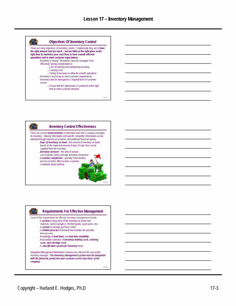
Inventory is such a major factor in a business operations that Counting Systems are necessary to ensure that inventory is being managed properly. Inventory systems are only as good as the information they contain … and transaction errors can be very costly.
. Periodic system - physical counts made at periodic intervals throughout the year
. Perpetual (continual) inventory systems - keep track of additions and removals from inventory so that a continual running total of inventory on hand is available
Most inventory systems today utilize “bar codes” to accurately track inventory movements easily and cost effectively.
. Grocery stores
. Retail stores
. Auto rentals
Inventory Counting Systems
17 - 11
The ABC method provides for classification of inventory according to some measure of importance (usually by annual dollar usage)
A - very important (accuracy within .2 percent)B - moderately important (accuracy within 1 percent)C - least important (accuracy within 5 percent)
Annual $ volumeof items
C
High
LowFew Many
Number of Items
The classification system does not necessarily mean that B and C items are unimportant from a production point of view. A stock-out of nuts and bolts which may be classified as C items can just as easily shut down a production line as a major component.
Classification Systems
BA
17 - 12
Example 1: Classify the inventory items below as A, B or C.
ABC Classification - Example
ItemAnnual
Demand Unit CostAnnual Dollar
Volume1 1,000 4,300 4,300,0002 5,000 720 3,600,0003 1,900 500 950,0004 1,000 710 710,0005 2,500 250 625,0006 2,500 192 480,0007 400 200 80,0008 500 100 50,0009 200 210 42,000
10 1,000 35 35,00011 3,000 10 30,00012 9,000 3 27,000
ItemAnnual
Demand Unit CostAnnual Dollar
Volume Classification1 1,000 4,300 4,300,000 A2 5,000 720 3,600,000 A3 1,900 500 950,000 B4 1,000 710 710,000 B5 2,500 250 625,000 B6 2,500 192 480,000 B7 400 200 80,000 C8 500 100 50,000 C9 200 210 42,000 C
10 1,000 35 35,000 C11 3,000 10 30,000 C12 9,000 3 27,000 C

Lesson 17 – Inventory Management
Copyright – Harland E. Hodges, Ph.D 17-5
17 - 13
How much and when to order depends on many factors including: ordering costs, carrying costs, lead times, variability in lead times, variability in demand, variability in production, etc..
The Economic Order Quantity (EOQ) is the order size (how much?) that minimizes the total cost of inventory.
The Reorder Point (ROP) is the inventory point (when?) which triggers a reorder.
How Much? When? To Order
How Much?When!
17 - 14
There are 3 Economic Order Quantity (EOQ) models which can be used to determine how much to order. Each has a scenario under which it is appropriate. They are:
. . Basic EOQ – instantaneous delivery
. EOQ – non-instantaneous delivery
. EOQ – quantity discount
How Much? To Order – EOQ Models
How Much?
17 - 15
Quantityon hand
Receive order
Time
Usage/demand rate
Placeorder
Receiveorder
Lead time
Reorderpoint
Q
Placeorder
Receiveorder
Time
Inventory Cycle – Instantaneous DeliveryInventory instantaneously increases by the quantity (Q) received.

Lesson 17 – Inventory Management
Copyright – Harland E. Hodges, Ph.D 17-6
17 - 16
The Basic Economic Order – instantaneous delivery model assumptions are as follows:
. Only one product is involved
. Demand requirements are known
. Demand is reasonably constant
. Lead time does not vary
. Each order is received in a single delivery (“instantaneously”)
. There are no quantity discounts
Basic EOQ – Instantaneous Delivery Model
17 - 17
Carrying Cost = Q2 H where
Q = Order quantityH = Holding (carrying) cost per unit
Basic EOQ – Carrying Cost
Annual Carrying Cost is linearly related to the Order Quantity
Order Quantity (Q)
Car
ryin
g C
ost
17 - 18
Ordering Cost = DQ S where
Q = Order quantityD = Demand, usually in unit per yearS = Ordering Cost
Ordering Cost decreases as Order Quantity increases;
however not linearly
Order Quantity (Q)
Ord
erin
g C
ost
Basic EOQ – Ordering Cost

Lesson 17 – Inventory Management
Copyright – Harland E. Hodges, Ph.D 17-7
17 - 19
Order Quantity (Q)
Tota
l Cos
t
SQDHQTC
TC
+=
+=
2
Cost Ordering Cost Carrying )(Cost Total
Basic EOQ – Total Cost
17 - 20
Basic EOQ
Tota
l Cos
t
Basic EOQ – Instantaneous DeliveryThe Basic Economic Order – instantaneous delivery model EOQ is the quantity which minimizes Total Cost = Carrying Cost + OrderingCost. It is where Carrying Cost = Order Cost and is calculated by:
Length of Order Cycle = QD
0
Basic EOQ = Q =2DS
H 0
17 - 21
Example 2a: A local distributor for a national tire company expects to sell 9,600 steel belted radial tires of a certain size and tread design next year. Annual Carrying Cost is $16 per tire, and Ordering Cost is $75. The distributor operates 288 days per year. What is the EOQ?
Econmic Order Quantity = Q =2DS
H
=2(9,600)(75)
16= 300
0
Basic EOQ – Example

Lesson 17 – Inventory Management
Copyright – Harland E. Hodges, Ph.D 17-8
17 - 22
Example 2b: How many times per year does the tire distributor reorder tires?
Number of Orders Per Year = DQ
=9,600300
= 320
Basic EOQ – Example
Example 2c: What is the length of the order cycle (Cycle Time)?
Length of Order Cycle = QD
=300
9,600=.03125
therefore since there are 288 days in the year the Order Cycle = .03125* 288 = 9 days
0
17 - 23
Example 2d: What is the Total Annual Cost if the EOQ is ordered?
TC Q2
HDQ
S
= $2,400 + $2,400 =
= + = +3002
169 600300
75
800
( ),
( )
$4,
Basic EOQ – Example
17 - 24

Lesson 17 – Inventory Management
Copyright – Harland E. Hodges, Ph.D 17-9
17 - 25
EOQ – Instantaneous Replenishment
17 - 26
Example 3a: Piddling Manufacturing assembles security monitors. It purchases 3,600 black and white cathode ray tubes (CRT’s) at $65 each. Ordering costs are $31, and annual carrying costs are 20% of the purchase price. Compute the optimal order quantity.
S = $31H = .20($65) = $13
Econmic Order Quantity = Q =2DS
H
=2(3,600)(31)
13= 131
0
Basic EOQ – Example
17 - 27
Example 3b: Compute the total annual ordering cost for the optimal order quantity.
TC Q2
HDQ
S
= $852 + $852 =
= + = +131
213
3 600131
31
704
( ),
( )
$1,
Basic EOQ – Example
Lesson 17 – Inventory Management
Copyright – Harland E. Hodges, Ph.D 17-10
17 - 28
EOQ – Instantaneous Replenishment
17 - 29
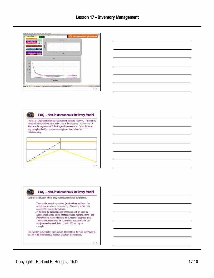
The basic EOQ model assumes instantaneous delivery; however, many times an organization produces items to be used in the assembly of products. In this case the organization is both a producer and user. Orders for items may be replenished (non-instantaneously) over time rather than instantaneously.
EOQ – Non-instantaneous Delivery Model
17 - 30
EOQ – Non-instantaneous Delivery ModelConsider the situation where a toy manufacturer makes dump trucks.
. The manufacturer also produces (production rate) the rubber wheels that are used in the assembly of the dump trucks. Let’s consider 500 per day for example.
. In this case the ordering costs associated with an order for rubber wheels would be the cost associated with the setup and delivery of the rubber wheels to the dump truck assembly area.
. The manufacturer makes the dump trucks at constant rate per day (production rate). Let’s consider 200 per day for example.
The inventory picture in this case is much different from the “saw-tooth” pattern we saw in the instantaneous model as shown on the next slide.
Lesson 17 – Inventory Management
Copyright – Harland E. Hodges, Ph.D 17-11
17 - 31
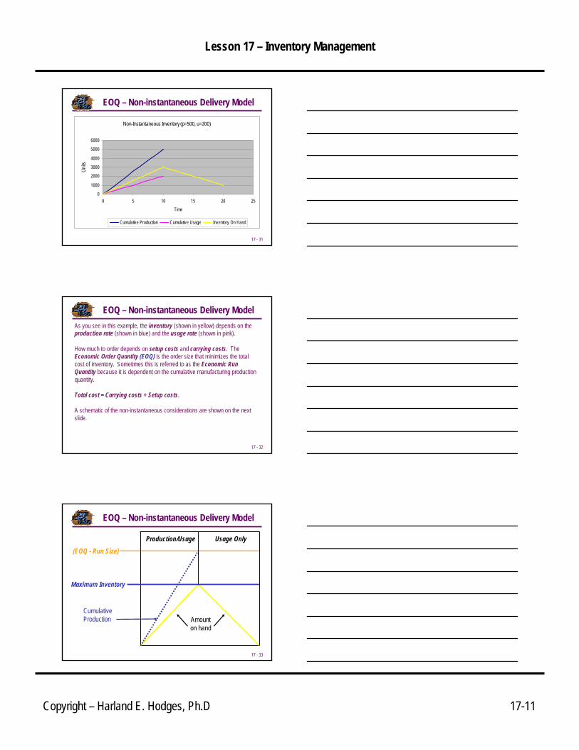
EOQ – Non-instantaneous Delivery Model
Non-Instantaneous Inventory (p=500, u=200)
0
1000
2000
3000
4000
5000
6000
0 5 10 15 20 25
Time
Units
Cumulative Production Cumulative Usage Inventory On Hand
17 - 32
EOQ – Non-instantaneous Delivery ModelAs you see in this example, the inventory (shown in yellow) depends on the production rate (shown in blue) and the usage rate (shown in pink).
How much to order depends on setup costs and carrying costs. The Economic Order Quantity (EOQ) is the order size that minimizes the total cost of inventory. Sometimes this is referred to as the Economic RunQuantity because it is dependent on the cumulative manufacturing production quantity.
Total cost = Carrying costs + Setup costs.
A schematic of the non-instantaneous considerations are shown on the next slide.
17 - 33
Maximum Inventory
(EOQ - Run Size) Production/Usage Usage Only
Amount on hand
Cumulative Production
EOQ – Non-instantaneous Delivery Model

Lesson 17 – Inventory Management
Copyright – Harland E. Hodges, Ph.D 17-12
17 - 34
Econmic Run Quantity = Q =2DS
Hp
p - u where
p = production rate u = usage rate S = ordering cost H = carrying cost D = annual demand
0
Maximum Inventory = I =Qp
(p- u)
Average Inventory = I
max0
max
2
EOQ – Non-instantaneous Delivery Model
17 - 35
Minimum Total Cost = TC = Carring Cost + Setup Cost
= I
H) + DQ
min
max
02( (S)
C yc le T im e = Qu
R u n T im e = Qp
0
0
EOQ – Non-instantaneous Delivery Model
17 - 36
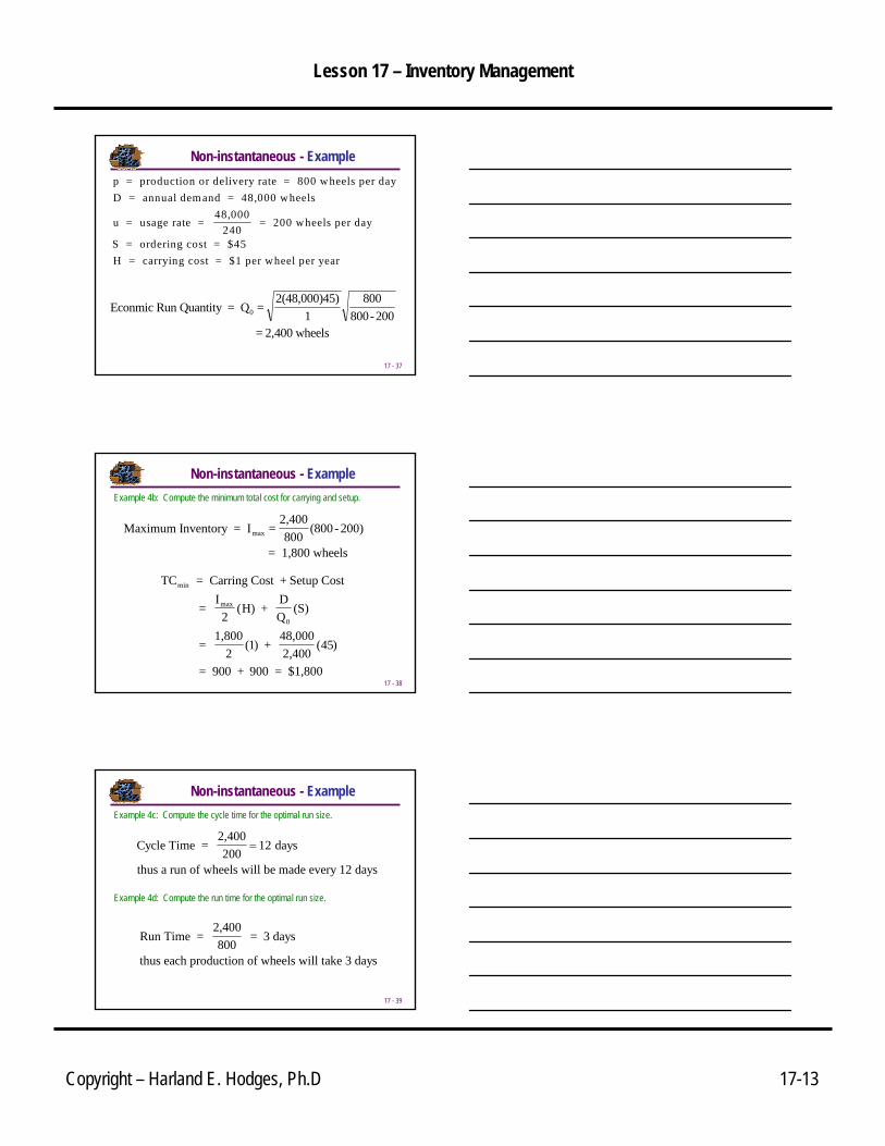
Example 4a: A toy manufacturer uses 48,000 rubber wheels per year for its popular dump truck series. The firm makes its own wheels, which it can produce at a rate of 800 per day. The toy trucks are assembled uniformly over the entire year. Carrying cost is $1 per wheel per year. Setup cost for a production run of wheels is $45. The firm operates 240 days per year. Determine the optimal run size.
Non-instantaneous - Example
Lesson 17 – Inventory Management
Copyright – Harland E. Hodges, Ph.D 17-13
17 - 37
Econmic Run Quantity = Q =2(48,000)45)
1800
800-200 = 2,400 wheels
0
Non-instantaneous - Examplep = production or delivery rate = 800 wheels per dayD = annual dem and = 48,000 wheels
u = usage rate = 48,000
240 = 200 wheels per day
S = ordering cost = $45H = carrying cost = $1 per wheel per year
17 - 38
Example 4b: Compute the minimum total cost for carrying and setup.
TC = Carring Cost + Setup Cost
= I
H) + DQ
= 1,800
) + 48,0002,400
)
= 900 + 900 = $1,800
min
max
02
21 45
( (S)
( (
Maximum Inventory = I =2,400800
(800 - 200)
= 1,800 wheels
max
Non-instantaneous - Example
17 - 39
Example 4c: Compute the cycle time for the optimal run size.
Cycle Time = 2,400200
days
thus a run of wheels will be made every 12 days
= 12
Example 4d: Compute the run time for the optimal run size.
Run Time = 2,400800
= 3 days
thus each production of wheels will take 3 days
Non-instantaneous - Example

Lesson 17 – Inventory Management
Copyright – Harland E. Hodges, Ph.D 17-14
17 - 40
17 - 41
EOQ – Non - Instantaneous Replenishment
17 - 42
EOQ with Quantity Discount is very important because price reductions are frequently offered to induce customers to order in larger quantities.
Why do you think this is done?
EOQ With Quantity Discount
In this model the purchasing cost will vary depending on the quantity purchased. Purchasing cost was omitted in the previous EOQ models because the price per unit was the same for all units; thus, the inclusion of the purchase cost would only increase the total cost function by the purchase cost amount. Thus, it would have had no effect on the EOQ calculation. This is illustrated in the next slide.

Lesson 17 – Inventory Management
Copyright – Harland E. Hodges, Ph.D 17-15
17 - 43
EOQ
Cost TC without Purchasing Cost
Quantity
Purchasing Cost – same for all units
TC with Purchasing Cost
EOQ Without Quantity Discount
Adding Purchasing costw/o quantity discountdoesn’t change EOQ
17 - 44
In this model, how much to order depends on purchase costs, setup costsand carrying costs. The Economic Order Quantity (EOQ) is the order size that minimizes the total cost of inventory. Sometimes this is referred to as the Economic Run Quantity because it is dependent on the cumulative manufacturing production quantity.
Total cost = Carrying costs + Ordering costs + Purchasing Cost
priceunit where2
Cost Purchasing Cost Ordering Cost Carrying )(Cost Total
=++=
++=
PPDSQDHQTC
TC
EOQ With Quantity Discount
17 - 45
The Method of Computing EOQ with Quantity Discount is a step wise process.
. First, compute the common EOQ using the earlier formula
. Second, .. Identify the price range where the common EOQ lies.. If the common EOQ is in the lowest quantity
range then the EOQ with quantity discount is the common EOQ
.. Otherwise, the EOQ with quantity discount is the quantity where the total cost is minimum when considering the cost for the common EOQ and the cost for all minimum quantities of price breaks greater than the common EOQ.
EOQ With Quantity Discount

Lesson 17 – Inventory Management
Copyright – Harland E. Hodges, Ph.D 17-16
17 - 46
Example 5a: The maintenance department of a large hospital uses 816 cases of liquid cleanser annually. Ordering costs are $12, carrying costs are $4 per case per year, and the price schedule for ordering is listed below. Determine the optimal order quantity and the total cost. There are 240 days in a year.
D = annual demand = 816 cases/ yearS = ordering cost = $12H = carrying cost = $4 per case per year
EOQ With Quantity Discount - Example
Order Quantity
Price Per Box
1 to 49 20.0050 to 79 18.0080 to 99 17.00
100 or more 16.00
17 - 47
Common EOQ = Q =2DS
H
=2(816)(12)
4= 70 cases
0
Common EOQ = 70
Is in the second price break
Order Quantity
Price Per Box
1 to 49 20.0050 to 79 18.0080 to 99 17.00
100 or more 16.00
EOQ With Quantity Discount - Example
17 - 48
Therefore; the
EOQ with quantity discount = minimum (TC(70), TC (80), TC (100))
Common EOQ = 70
Is in the second price break
Order Quantity
Price Per Box
1 to 49 20.0050 to 79 18.0080 to 99 17.00
100 or more 16.00
EOQ With Quantity Discount - Example

Lesson 17 – Inventory Management
Copyright – Harland E. Hodges, Ph.D 17-17
17 - 49
TC 702
(4) + 81670
12 + 18(816) = $14,96870 =
TC 802
(4) + 81680
12 + 17(816) = $14,15480 =
TC 1002
(4) + 816100
12 + 16(816) = $13,354100 =
Therefore; the total cost is minimum for an order quantity of 100 and the
EOQ with quantity discount = 100
EOQ With Quantity Discount - Example
17 - 50
17 - 51
EOQ – Quantity Discount

Lesson 17 – Inventory Management
Copyright – Harland E. Hodges, Ph.D 17-18
17 - 52
The Reorder Point (ROP) is the quantity of inventory on hand that triggers a reorder. Four determinants for a reorder point
. Rate of demand (based on a forecast)
. Lead time
. Extent of demand and lead time variability
. Degree of stock out risk acceptable
The ROP calculation will depend on thethe variability situation
. Variability in demand
. Variability in lead time
. Variability in demand & lead time
When To Reorder
When!
17 - 53
If demand and lead time are both constant the Reorder Point (ROP)can be calculated by the following formula:
ROP d(LT) where d = demand rate (units per day or week) LT = lead time in days or weeks
=
ROP - Constant Demand & Lead Time
17 - 54
Example 7: Tingly takes a “Two-A-Day” vitamins, which are delivered to his home by a route man seven days after the order is called in. At what point should Tingly reorder?
d = demand rate (units per day or week) = 2 / dayLT = lead time in days or weeks = 7 days
ROP 2(7) = 14 vitamins=
ROP - Constant Demand & LT - Example

Lesson 17 – Inventory Management
Copyright – Harland E. Hodges, Ph.D 17-19
17 - 55
If variability in demand or lead time is present the ROP is calculated using the following general formula. 3 specific formula will follow depending upon what is variable (demand, lead time, demand & lead time):
ROP Expected demand during lead time + Safety Stock=
Safety Stock - stock that is held in excess of expected demand due to the variability in demand rate and/or lead time
For example: If the expected demand during lead time is 100 units and the desired amount of safety stock is 10 units then
ROP = 100 + 10
When To Reorder
17 - 56
It is rarely the case in business where demand & lead time are constant. Variability can exist because of many reasons (customers, transportation, etc.); therefore, we must consider these impacts on inventory.
ROP - Demand & Lead Time Variability
Quantityon hand
Receive order
Time
Q
Placeorder
Receiveorder
Lead time 1
Reorderpoint
Placeorder
Receiveorder
Lead time 2
Receiveorder
Lead time 3
Placeorder
Usage/demand rate
17 - 57
The calculation of safety stock depends on the variability of demand, lead time and the service level the organization desires.
Service Level – is the proportion of customer orders that are serviced on-time. Customers usually understand that 100% of their orders will not be serviced on-time and will establish standards for service.
By developing a probability distribution of demand during lead time, a company can use statistical calculations which determine how much safety stock is necessary to meet customer service requirements. In this case, the supply of inventory on hand a company must have to meet customer requirements is calculated by supply (inventory on hand) = expected demand + safety stock. This is depicted on the next slide.
Safety Stock

Lesson 17 – Inventory Management
Copyright – Harland E. Hodges, Ph.D 17-20
17 - 58
Probability distribution of quantity of demand
during lead time
Expecteddemand
Safety Stock
Risk ofa stock out“Service Level”
probability of no stock out
Safety Stock
17 - 59
When variability in demand and/or lead time are present, and the standard deviation of the demand during lead time can be calculated; Safety Stockis calculated using the following formula:
demand timelead ofdeviation standard the= level service deisred theachieve tonecessary
deviations standard ofnumber = =Stock Safety
dLT
dLT
σ
σz
z
Safety Stock
17 - 60
Example 8: Suppose that a manager of construction supply house determined from historical records that demand for sand during lead time averages 50 tons. In addition, suppose the manager determined that demand during lead time could be described by a normal distribution that has a mean of 50 tons and a standard deviation of 5 tons. Answer the following questions assuming the manager is willing to accept a stock out risk of no more than 3%.
Example 8a: What value of z is appropriate?
The risk of a stock out is .03; therefore, the service level (probability of no stock out) is .97. We can look this up in the standard normal distribution tables to calculate this number. Z(97%) = 1.881.
ROP - Variable Demand & LT - Example

Lesson 17 – Inventory Management
Copyright – Harland E. Hodges, Ph.D 17-21
17 - 61
Example 8b: How much safety stock should be held?
Safety Stock = = 1.88(5) = 9.40 tons dLTzσ
Example 8c: What reorder point should the manager use?
ROP Expected demand during lead time + Safety Stock = 50 + 9.40 = 59.40 tons
=
ROP - Variable Demand & LT - Example
17 - 62
In the previous example, we were given the demand during lead time. When data on lead time demand are not readily available, we must determine the demand during lead time (which will depend on where variability exists). In this case there are 3 different formula for calculating the reorder point (ROP). The formula will depend on the variability situation.
. Only variability in demand
. Only variability in lead time
. Both demand & lead time are variable
Other Considerations
17 - 63
If only demand is variable then the following formula is used to calculate the ROP.
ROP Expected demand during lead time + Safety Stock
= d(LT) + LT( ) where d = average daily or weekly demand = standard deviation of the demand per day or week LT = lead time in days or weeks
d
d
=
z σ
σ
ROP – Variability In Demand

Lesson 17 – Inventory Management
Copyright – Harland E. Hodges, Ph.D 17-22
17 - 64
or weeks daysin timelead theofdeviation standard = demandor weekly daily = d
whered + Time) Lead (average*d = StockSafety + timelead during demand Expected ROP
LT
LT
σ
σz=
If only lead time is variable then the following formula is used to calculate the ROP.
ROP – Variability In Lead Time
17 - 65
If both lead time and demand are variable then the following formula is used to calculate the ROP.
ROP Expected demand during lead time + Safety Stock
= d(avearge Lead Time) + average Lead Time) d where d = average daily or weekly demand
= variance of demand in days or weeks = variance of lead time in days or weeks
d2 2
LT2
d2
d2
=
+z ( σ σ
σ
σ
ROP – Variability In Demand & Lead Time
17 - 66
As you can see, inventory management can be fairly complicated because of all of the scenarios that are possible. Using the correct quantitative tools to manage this very critical component of a business “cash flow” can reap great rewards.
Inventory Management
End Product
E(1)
The process even becomes more complicated when we realize that an end product (dependent demand)is made up of components(independent demand) and that inventory must be managed at the component level as well as the end product level.

Lesson 17 – Inventory Management
Copyright – Harland E. Hodges, Ph.D 17-23
17 - 67
HomeworkRead and understand all material in the chapter.
Discussion and Review Questions
Recreate and understand all classroom examples
Exercises on chapter web page
Related Documents