),1,7((/(0(17 02'(/,1* 2) +<%5,' &20326,7( %($0 %5,'*( ,1 9,5*,1,$ 7,'(6 0,// 675($0 %5,'*( $ 7KHVLV 3UHVHQWHG WR WKH IDFXOW\ RI WKH 6FKRRO RI (QJLQHHULQJ DQG $SSOLHG 6FLHQFH 8QLYHUVLW\ RI 9LUJLQLD LQ SDUWLDO IXOILOOPHQW RI WKH UHTXLUHPHQWV IRU WKH GHJUHH 0DVWHU RI 6FLHQFH E\ +DR]KH <L $XJXVW

Welcome message from author
This document is posted to help you gain knowledge. Please leave a comment to let me know what you think about it! Share it to your friends and learn new things together.
Transcript

),1,7(�(/(0(17�02'(/,1*�2)�+<%5,'�&20326,7(�%($0�%5,'*(�,1�9,5*,1,$��7,'(6�
0,//�675($0�%5,'*(
$�7KHVLV
3UHVHQWHG�WR
WKH�IDFXOW\�RI�WKH�6FKRRO�RI�(QJLQHHULQJ�DQG�$SSOLHG�6FLHQFH
8QLYHUVLW\�RI�9LUJLQLD�
LQ�SDUWLDO�IXOILOOPHQW
RI�WKH�UHTXLUHPHQWV�IRU�WKH�GHJUHH�
0DVWHU�RI�6FLHQFH
E\
+DR]KH�<L
$XJXVW������

i
FINITE-ELEMENT MODELING OF HYBRID COMPOSITE BEAM
BRIDGE IN VIRGINIA: TIDES MILL STREAM BRIDGE
Haozhe Yi
ABSTRACT
The Hybrid Composite Beam (HCB), an innovative composite shell/reinforced
concrete beam, was used as part of the replacement of the superstructure of the Tides Mill
Stream Bridge on Route 205 in Colonial Beach, Virginia. A series of load tests were
conducted on the completed replacement structure in order to validate the design
assumptions and to characterize the overall structural response of the bridge. A detailed
finite element model of the bridge was developed in order to further understand the
behavior of this unique bridge. Finite element modeling has been widely used to conduct
structural analysis on bridges for many years. However, because of the novelty of the HCB,
finite element modeling has only been used in limited analyses on HCB bridges (Myers,
2015). This study aimed to develop a rational finite element model to simulate the behavior
of the Tides Mill Stream Bridge under static and dynamic loads. Results from a laboratory
study conducted at Virginia Tech (Ahsan, 2012) were used to calibrate a finite element
model of the HCB beam. A three beam/concrete deck bridge system, also tested at Virginia
Tech, was used to calibrate a finite element model of the tested bridge system. A full finite
element model of the Tides Mill Stream Bridge was developed. Results from field testing
conducted on the completed Tides Mill Stream Bridge, by the University of Virginia, were
used as benchmarks to adjust the full finite element bridge model. The proposed finite
element model developed in this study was able to predict the behavior of the Tides Mill

ii
Stream Bridge with acceptable accuracy. This finite element model can be used as a
reference for future analyses on the Tides Mill Stream Bridge.

iii
ACKNOWLEDGEMENT
I would like to thank Dr. Jose Gomez, Dr. Devin Harris, and Dr. Osman Ozbulut
for serving as the committee members of my defense.
I deeply appreciate the opportunity to be involved in the research of Dr. Devin
Harris and receiving the guidance and support from Dr. Devin Harris and Dr. Jose Gomez
during my stay at the University of Virginia. I would like to greatly thank Dr. Jose
Gomez for accepting me as his student, and for his input, patience and endless support.
iv
Table of Content
1 Introduction ................................................................................................................. 1
1.1 Project Description and Overview ...................................................................... 1
1.2 Thesis Objective.................................................................................................. 2
1.3 Thesis Outline ..................................................................................................... 2
2 Literature Review ....................................................................................................... 4
2.1 Previous Studies on Modeling Bridge Components made of FRP or GFRP ...... 5
2.2 Previous Studies on Modeling Hybrid Composite Beam Bridges ...................... 6
2.3 Previous Studies on HCB Bridges ...................................................................... 8
2.4 Summary ........................................................................................................... 10
3 Initial Model Development ....................................................................................... 11
3.1 Summary of Experimental Program ................................................................. 11
3.2 Geometry of Model ........................................................................................... 16
3.3 Materials Properties of the Model .................................................................... 18
3.4 Model Construction and Analysis ..................................................................... 20
3.4.1 HCB Model without Arch ........................................................................... 21
3.4.2 Full HCB Model ......................................................................................... 24
3.4.3 Three Beam/Composite Deck Model.......................................................... 39
3.4.4 Model of Tides Mill Stream Bridge ............................................................ 47
4 Results and Discussion ............................................................................................. 59

v
4.1 HCB Model without Arch ................................................................................. 59
4.2 Full HCB Model ............................................................................................... 63
4.2.1 Discussion about Contact Conditions ......................................................... 63
4.2.2 Refinement of HCB Model ......................................................................... 63
4.2.3 Results of Full HCB Model ........................................................................ 66
4.3 Three Beam/Composite Deck Model................................................................ 72
4.4 Model of Tides Mill Stream Bridge .................................................................. 79
4.4.1 Simplifications ............................................................................................ 79
4.4.2 Modification on Open Deflection Joints ..................................................... 79
4.4.3 Refinement on Semi-Integral Backwalls .................................................... 79
4.4.4 Accuracy of Bridge Model.......................................................................... 81
4.4.5 Load Case A ................................................................................................ 81
4.4.6 Load Case B ................................................................................................ 84
4.4.7 Load Case C ................................................................................................ 87
4.4.8 Load Case D ................................................................................................ 90
4.4.9 Load Case E ................................................................................................ 93
4.4.10 Load Case F ................................................................................................ 95
4.4.11 Comparison of Frequencies of First Modes ................................................ 97
5 Conclusions and Recommendations ......................................................................... 98
5.1 Conclusions ....................................................................................................... 98

vi
5.2 Recommendations ............................................................................................. 99

vii
List of Tables
Table 3-1 Dimension of Main Components (Slade & Eriksson, 2012) ............................ 17
Table 3-2 Material Properties of FRP (Slade & Eriksson, 2012) ..................................... 18
Table 3-3 Material Properties of Other Components (Ahsan, 2012) ................................ 19
Table 3-4 Paths of HCB Model ........................................................................................ 30
Table 3-5 Paths of Three HCBs System Model ................................................................ 42
Table 3-6 Paths of Bridge Model ...................................................................................... 53
Table 4-1 Mid-Span Deflection for HCB without Arch ................................................... 60
Table 4-2 Mid-Span Strains for Tests 7 (HCB without Arch) .......................................... 61
Table 4-3 Quarter Strains for Tests 7 (HCB without Arch) .............................................. 62
Table 4-4 Strains of Model, Refined Model, and VT’s Tests ........................................... 65
Table 4-5 Promotion of HCB Model after Refinement .................................................... 65
Table 4-6 Mid-Span Deflection for Point Load Tests ...................................................... 66
Table 4-7 Mid-Span Deflection for Quarter Point Load Tests ......................................... 67
Table 4-8 Mid-Span Strain for Point Load Tests .............................................................. 68
Table 4-9 Quarter Point Strains for Quarter Point Load Tests ......................................... 69
Table 4-10 Mid-Span Strains in Top-Arch for Point Load Tests ..................................... 70
Table 4-11 Mid-Span Strain in Top-Arch for Quarter Point Load Tests .......................... 71
Table 4-12 Maximum FRP Strain in Bottom Flange ........................................................ 72
Table 4-13 Deflections of Three HCBs at Bottom Flange ............................................... 74
Table 4-14 Maximum Arch Strains of Three HCBs ......................................................... 76
Table 4-15 Promotion of Bridge Model after Refinement................................................ 79
Table 4-16 Average Deviation of Strain at Mid-Span ...................................................... 81
viii
Table 4-17 Mid-Span Strains at Tension Level ................................................................ 81
Table 4-18 Mid-Span Strains through Bridge Depth ........................................................ 82
Table 4-19 Mid-Span Strains at Tension Level ................................................................ 84
Table 4-20 Mid-Span Strains through Bridge Depth ........................................................ 85
Table 4-21 Mid-Span Strains at Tension Level ................................................................ 87
Table 4-22 Mid-Span Strains through Bridge Depth ........................................................ 88
Table 4-23 Mid-Span Strains at Tension Level ................................................................ 90
Table 4-24 Mid-Span Strains through Bridge Depth ........................................................ 91
Table 4-25 Mid-Span Strains at Tension Level ................................................................ 93
Table 4-26 Mid-Span Strains through Bridge Depth ........................................................ 94
Table 4-27 Mid-Span Strains at Tension Level ................................................................ 95
Table 4-28 Mid-Span Strains through Bridge Depth ........................................................ 96
Table 4-29 Natural Frequencies of First Five Modes ....................................................... 97

ix
List of Figures
Figure 1-1 HCB Design (Harris, Civitillo, & Gheitasi, 2016) ............................................ 1
Figure 2-1 Comparison of the B0439 Deflections Measured at the Field and Predicted by
ANSYS, SAP2000, and Theoretical Calculations (Myers, 2015) ...................................... 7
Figure 2-2 Typical Cross Section of Bridge B0439 (Myers, 2015) .................................... 8
Figure 3-1 Instrumentation of HCB (Ahsan, 2012) .......................................................... 12
Figure 3-2 Uniform Load on HCB without Arch (Ahsan, 2012) ..................................... 12
Figure 3-3 Load Cases of Full HCB Tests (Ahsan, 2012) ................................................ 13
Figure 3-4 Load Cases of Three HCB/Composite Deck System Tests (Ahsan, 2012) .... 14
Figure 3-5 Instrumentation of Tides Mill Stream Bridge ................................................. 15
Figure 3-6 Load Cases of Tests on Tides Mill Stream Bridge ......................................... 15
Figure 3-7 Typical Section of Bridge Model .................................................................... 16
Figure 3-8 Plan View of HCBs Model ............................................................................. 16
Figure 3-9 Shell and Bottom Strands ................................................................................ 21
Figure 3-10 Distributed Load of 2125 pounds .................................................................. 22
Figure 3-11 Concentrated Load of 250 pounds at Mid-Span ........................................... 23
Figure 3-12 Model of HCB ............................................................................................... 24
Figure 3-13 Model of Arch ............................................................................................... 25
Figure 3-14 Model of Bottom Strands .............................................................................. 26
Figure 3-15 Model of Embedded Strands in Arch ............................................................ 26
Figure 3-16 Model of Shear Connectors ........................................................................... 27
Figure 3-17 Model of Shell ............................................................................................... 27
Figure 3-18 Model of Added Surface ............................................................................... 29
x
Figure 3-19 Details of Cross Sections .............................................................................. 29
Figure 3-20 Plan View of Paths on HCB Model .............................................................. 30
Figure 3-21 Locations of Paths on HCB Model (Side Elevation View)........................... 31
Figure 3-22 Mesh Result of Full HCB Beam ................................................................... 34
Figure 3-23 Details of “Patch Conforming Method” ........................................................ 35
Figure 3-24 Details of “Mesh” .......................................................................................... 35
Figure 3-25 Concentrated Load of 15 kips at Mid-Span .................................................. 37
Figure 3-26 Concentrated Load of 25 kips at quarter spans ............................................. 37
Figure 3-27 Separated Bottom Shell ................................................................................. 38
Figure 3-28 Model of Three HCBs System ...................................................................... 39
Figure 3-29 Deck Setback 7 Inches for Framework ......................................................... 40
Figure 3-30 Model of Deck on Three HCBs .................................................................... 41
Figure 3-31 Model of Added Surfaces.............................................................................. 42
Figure 3-32 Locations of Paths on Three HCBs System Model (Side Elevation View) .. 43
Figure 3-33 Paths of Three HCBs System Model ............................................................ 43
Figure 3-34 Eight Load Cases of Three HCBs System Model ......................................... 45
Figure 3-35 Load Case Configurations of Three HCBs System....................................... 46
Figure 3-36 Model of Tides Mill Stream Bridge .............................................................. 47
Figure 3-37 Model of Bridge Deck ................................................................................... 48
Figure 3-38 Model of Bridge Parapets.............................................................................. 49
Figure 3-39 Model of Bridge Backwalls .......................................................................... 49
Figure 3-40 Illustration of HCB Beam (G5) Embedded into Backwalls .......................... 50
Figure 3-41 Model of Added Surfaces on Bridge ............................................................. 51
xi
Figure 3-42 Parapet with Open Deflection Joints ............................................................. 52
Figure 3-43 Open Deflection Joint ................................................................................... 52
Figure 3-44 Paths of Bridge Model .................................................................................. 54
Figure 3-45 Locations of Paths on Bridge Model (West Side Elevation View) ............... 54
Figure 3-46 Simply Supported Support at Western Backwall (Bottom View) ................ 55
Figure 3-47 Displacement Support at Eastern Backwall (Bottom View) ......................... 55
Figure 3-48 Six Load Cases of Bridge Model .................................................................. 56
Figure 3-49 Load Case Configurations of Tides Mill Stream Bridge .............................. 57
Figure 4-1 Mid-Span Deflection for HCB without Arch .................................................. 60
Figure 4-2 Mid-Span Strains for Tests 7 (HCB without Arch) ........................................ 61
Figure 4-3 Quarter Strains for Tests 7 (HCB without Arch) ............................................ 62
Figure 4-4 Change of Modulus of Elasticity in Bottom Flange........................................ 64
Figure 4-5 Comparison of Strains through HCB Depth ................................................... 64
Figure 4-6 Mid-Span Deflection for Point Load Tests ..................................................... 66
Figure 4-7 Mid-Span Deflection for Quarter Point Load Tests ........................................ 67
Figure 4-8 Mid-Span Strain for Point Load Tests ............................................................ 68
Figure 4-9 Quarter Point Strain for Quarter Point Load Tests.......................................... 69
Figure 4-10 Mid-Span Strain in Top-Arch for Point Load Tests...................................... 70
Figure 4-11 Mid-Span Strain in Top-Arch for Quarter Point Load Tests ........................ 71
Figure 4-13 Maximum FRP Strain in Bottom Flange ...................................................... 73
Figure 4-14 Deflections of Three HCBs at Bottom Flange .............................................. 75
Figure 4-15 Maximum Arch Strains of Three HCBs (inconsistent values not shown) .... 77

xii
Figure 4-16 Comparison of Performance of Bridge Model before and after Placement of
Semi-Integral Backwalls ................................................................................................... 80
Figure 4-17 Plan View of Total Deflection for Load Case A ........................................... 81
Figure 4-18 Mid-Span Strains at Tension Level ............................................................... 82
Figure 4-19 Mid-Span Strains through Bridge Depth in G5 (upper left), G7 (upper right),
and G8 (bottom) ................................................................................................................ 83
Figure 4-20 Plan View of Total Deflection for Load Case B ........................................... 84
Figure 4-21 Mid-Span Strains at Tension Level ............................................................... 85
Figure 4-22 Mid-Span Strains through Bridge Depth in G5 (upper left), G7 (upper right),
and G8 (bottom) ................................................................................................................ 86
Figure 4-23 Plan View of Total Deflection for Load Case C ........................................... 87
Figure 4-24 Mid-Span Strains at Tension Level ............................................................... 88
Figure 4-25 Mid-Span Strains through Bridge Depth in G5 (upper left), G7 (upper right),
and G8 (bottom) ................................................................................................................ 89
Figure 4-26 Plan View of Total Deflection for Load Case D ........................................... 90
Figure 4-27 Mid-Span Strains at Tension Level ............................................................... 91
Figure 4-28 Mid-Span Strains through Bridge Depth in G5 (upper left), G7 (upper right),
and G8 (bottom) ................................................................................................................ 92
Figure 4-29 Plan View of Total Deflection for Load Case E ........................................... 93
Figure 4-30 Mid-Span Strains at Tension Level ............................................................... 93
Figure 4-31 Mid-Span Strains through Bridge Depth in G5 (upper left), G7 (upper right),
and G8 (bottom) ................................................................................................................ 94
Figure 4-32 Plan View of Total Deflection for Load Case F ........................................... 95

xiii
Figure 4-33 Mid-Span Strains at Tension Level ............................................................... 95
Figure 4-34 Mid-Span Strains through Bridge Depth in G5 (upper left), G7 (upper right),
and G8 (bottom) ................................................................................................................ 96
Figure 4-35 First Five Mode Shapes ................................................................................. 97
1
1 Introduction
1.1 Project Description and Overview
The Tides Mill Stream Bridge is located on Route 205 in Colonial Beach,
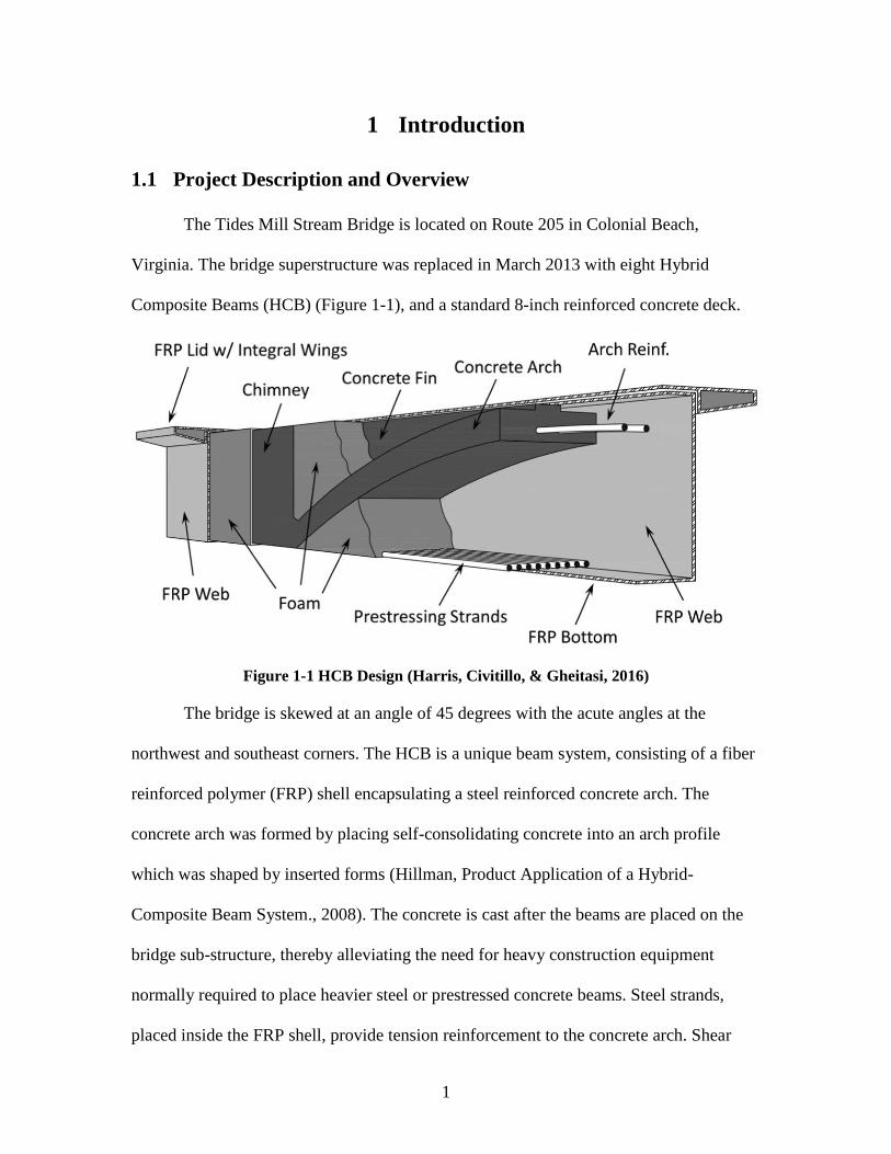
Virginia. The bridge superstructure was replaced in March 2013 with eight Hybrid
Composite Beams (HCB) (Figure 1-1), and a standard 8-inch reinforced concrete deck.
Figure 1-1 HCB Design (Harris, Civitillo, & Gheitasi, 2016)
The bridge is skewed at an angle of 45 degrees with the acute angles at the
northwest and southeast corners. The HCB is a unique beam system, consisting of a fiber
reinforced polymer (FRP) shell encapsulating a steel reinforced concrete arch. The
concrete arch was formed by placing self-consolidating concrete into an arch profile
which was shaped by inserted forms (Hillman, Product Application of a Hybrid-
Composite Beam System., 2008). The concrete is cast after the beams are placed on the
bridge sub-structure, thereby alleviating the need for heavy construction equipment
normally required to place heavier steel or prestressed concrete beams. Steel strands,
placed inside the FRP shell, provide tension reinforcement to the concrete arch. Shear
2
reinforcement is also in place prior to casting of the concrete arch. The shear
reinforcement extends through the top of the HCB to provide horizontal shear transfer
between the cast-in-place deck and the HCB beams, thus insuring composite action
between the HCB beams and the bridge deck. Internal sensors were installed inside the
bridge during the fabrication for research purpose.
This study depended on previous researches conducted by Virginia Tech and the
University of Virginia. To build a rational bridge model, the results from experimental
testing at Virginia Tech and the collected data from field testing by the University of
Virginia were used as benchmarks to validate the accuracy of models in this study.
1.2 Thesis Objective
The goal of this study was to develop a detailed finite element model of the Tides
Mill Stream Bridge. A detailed finite element model of the HCB beam was first
developed and calibrated from results reported by Virginia Tech on full-scale structural
testing of the individual HCB beam. Next a three beam/composite concrete deck finite
element model was developed and calibrated using results from a full-scale test, again
conducted at Virginia Tech (Ahsan, 2012). Finally, a finite element model of the Tides
Mill Stream Bridge was developed and calibrated, using results from static and dynamic
field testing on the completed Tides Mill Stream Bridge, conducted by the University of
Virginia.
1.3 Thesis Outline
Chapter 2 presents a summary and review of literature relevant to this thesis.
Chapter 3 provides details of the methodological approach to the development of the
finite element model of the Tides Mill Stream Bridge. Chapter 4 presents comparisons of

3
the finite element models to experimental results. Chapter 5 concludes with a summary
and recommendations for further study.

4
2 Literature Review
Fiber reinforced polymer (FRP) composite materials are progressively used in
civil engineering projects (Cai, Oghumu, & Meggers, 2009). The HCB is an efficient
combination of glass fiber reinforced polymer and conventional materials such as
concrete and steel (Hillman, Product Application of a Hybrid-Composite Beam System.,
2008). This new type of beam was designed to provide necessary strength and stiffness
with a lighter self-weight compared with concrete and steel beams of similar size and
load carrying capacity. The light weight results from the reduced quantity of concrete
required to meet the design strength and stiffness, which is both economical and
environmentally friendly. Also the shipping costs may be reduced based on the fact of
lighter weight, especially when the beams are shipped before placement of the concrete
arch. Another advantage of the light weight of the HCB is that existing abutments can be
reused for bridge replacement. The HCB is able to support its self-weight and the weight
of the uncured concrete. Thus it can be placed on the abutments prior to placing of the
arch concrete and no shoring is needed during the construction (Hillman, Investigation of
a Hybrid-Composite Beam System, 2003). An HCB bridge structure can be easily
constructed by state forces using typical state force equipment (no need to rent
large/high-cost cranes). Furthermore, the FRP shell is able to protect the internal
components from corrosion and damage and potentially extend the lifespan to
approximately 100 years versus approximately 75 years for the conventional concrete
beams (Civitillo, 2014). The FRP composite material also weathers marine environments.
5
2.1 Previous Studies on Modeling Bridge Components made of FRP or
GFRP
Machado et al. studied a finite element modeling technique for honeycomb FRP
bridge decks which have been used for rehabilitating highway bridges in the United
States. The complex geometry of honeycomb FRP decks and computational limits
prevented modeling the decks in detail. To solve this problem, the proposed modeling
technique provided a workable tool to model the complicated geometry of honeycomb
FRP bridge decks. The modeling of other components of the bridges were also introduced
in this study.
Tuwair et al. developed analytical models of glass fiber-reinforced polymer
(GFRP) bridge deck panels, and conducted finite element analyses on these models. The
deck panels were composed of two GFRP sheets and trapezoidal-shaped low-density
polyurethane foam segments separated by webs made of E-glass-woven fabric. These
panels shown better performance than regular sandwich panels on flexural stiffness,
strength, and shear stiffness. The critical sheet winkling of the panels was predicted using
analytical models. A 3D model was constructed to analyze the panel system under four-
point static loading. The behavior of the finite element model agreed with that of the
experimental testing in a good manner. The flexural strength of the sandwich panel was
predicted using a flexural beam theory. The effects of the deck panel components were
evaluated by conducting a parametric study.
Cai et al. developed equivalent properties for a complicated sandwich panel
utilizing the finite element modeling techniques. The sandwich panel were used for FRP
bridge decks to meet the necessary stiffness and to reduce the self-weight at the same
6
time. The hollowed sandwich panel can be transformed into a solid orthotropic plate
which has equivalent properties with the original sandwich panel. The deflection limits
can be evaluated and designed by analyzing the equivalent plate. The in-plane axial
properties of the sandwich core was first been developed, then the out-of-plane panel
properties for bending behavior of the panel was established. The contribution of wearing
surface to the stiffness of bridges with FRP panels was investigated. In the conventional
design of bridges with traditional deck systems, the contribution of wearing surface was
not usually counted in.
2.2 Previous Studies on Modeling Hybrid Composite Beam Bridges
Myers et al. modeled the Bridge B0439, a three-span hybrid composite beam
bridge completed in November 2011 in Missouri, using two commercial finite element
analysis (FEA) packages (ANSYS and SAP2000), and examined the accuracy of linear
FEA in predicting the static behavior of the HCB under service loads. Load testing was
performed on the bridge, and the deflections of the HCB beams were measured at
different locations. The transformed area method was used to theoretically calculate the
deflections of HCB beams. The measured deflections and the theoretical calculations
were compared with the predicted deflections of the finite element models.

7
e
Figure 2-1 Comparison of the B0439 Deflections Measured at the Field and Predicted by
ANSYS, SAP2000, and Theoretical Calculations (Myers, 2015)
As can be seen in Figure 2-1, the deflections of two finite element models were
close to the measured deflections, whereas the deflections from theoretical calculation
were generally larger than the measured deflections. The comparison proved that the
FEA can predict the behavior of the HCB Bridge with acceptable accuracy.

8
Figure 2-2 Typical Cross Section of Bridge B0439 (Myers, 2015)
2.3 Previous Studies on HCB Bridges
Harris et al. investigated the Tides Mill Stream Bridge located on Route 205 in
Colonial Beach, Virginia. The in-service performance of this bridge was evaluated by
acquiring data from a series of internal and external strain gauges. Tandem axle dump
trucks were used to perform both quasi-static and dynamic tests. Lateral load distribution,
internal load-sharing behavior, and dynamic load allowance were determined in the
experimental investigation. The HCB system performed close to the beam-type bridges
described in the AASHTO specifications when considering the live load performance, but
this system also reflected some features of a flexible system when considering the
dynamic response. The internal load-sharing behavior was found to be noncomposite and
even nonlinear, which indicating that the components within the HCB system can behave
independently. Local arch bending and slide between the tension strands and the resin
matrix could be the reasons of this phenomena.
Ahsan introduced the evaluation of HCB for use in the Tides Mill Stream Bridge.
An individual HCB and a three-HCB-system was tested and examined at Virginia Tech
to validate the current design methodology and the simplifying assumptions used in
HCB. The experimental results of the FRP shell and the tension strands were consistent
with the predicted behavior. The arch was found to be easily affected by local bending so

9
that it can performed in a very different way from the predicted behavior. In general, the
HCB behaved linearly. Small non-linear behavior happened in the beams under the
design live load. The distribution factors from AASHTO were conservative for exterior
girders compared with those from testing, but were not conservative for interior girders.
The distribution factors from Hillman’s model were conservative for both exterior and
interior girders. The current design methodology was shown to be good at predicting the
behavior of FRP shell and strands. However, the arch behaved far differently from the
prediction.
Thomas Snape et al. reported the testing of the HCB for the Knickerbocker
Bridge. The Maine Department of Transportation (MDOT) intended to replace the
Knickerbocker Bridge utilizing the HCB system in 2009. A full-scale HCB manufactured
by Harbor Technologies, Inc. was tested in AEWC laboratory. The test program was
consisted of fabricating one beam unit, placing it in the AEWC lab, pouring the SCC in
the arch, and casting a concrete deck on it. The composite HCB behaved well through the
important period of filling the arch concrete. The initial deflections caused by the fluid
load of the concrete of the arch and the deck generally agreed with the design
calculations except that the beam experienced a negative camber of approximately 1 3/8
inches at mid-span immediately prior to static testing. The HCB is linear-elastic under the
design loading, and John Hillman’s analytical model is accurate in predicting behavior of
beam under service loads. The fatigue tests showed that no deterioration or degradation
was investigated in the HCB under service load and following 2,000,000 fatigue bending
cycles. Almost all of the measured mechanical properties increased after the weathering
treatment.

10
2.4 Summary
Numerous studies have been conducted on modeling regular type of bridges, and
a number of studies have been performed on modeling bridge components consisting of
FRP or GFRP composite materials. Because of the novelty of the HCB, however, limited
studies have been developed on modeling HCB bridges.
This study aimed to develop a rational finite element model to simulate the
behavior of the Tides Mill Stream Bridge. The results from laboratory testing at Virginia
Tech and field testing of the completed bridge by the University of Virginia were used as
benchmarks to calibrate the models in this study.

11
3 Initial Model Development
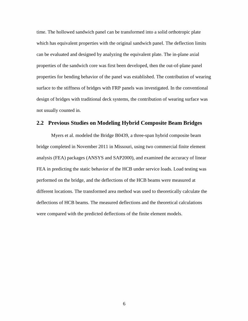
3.1 Summary of Experimental Program
The individual HCB without concrete arch was tested at Virginia Tech before the
testing of the full individual HCB. A system consisted of the shell and the bottom strands
was tested to better understand the behavior of these two components. The FRP lid was
not attached prior to shipping to Virginia Tech to facilitate the placement of
instrumentation prior to testing. The instrumentation of the test HCB is shown in Figure
3-1. The lid was attached to the FRP box with epoxy and screws after the instrumentation
was placed. Pin and roller supports were placed at 6 inches from the beam ends at a clear
span of 43 feet in order to simulate the span length of the Tides Mill Stream Bridge. Steel
angles (each weighing 25 pounds) were placed on the top of the HCB to provide a
uniform load across the span. Three HCBs, designated HCB1, HCB2, and HCB3 were
tested. For HCB1, a total of 85 steel angles, were evenly placed across the span length
resulting in a uniform load of 2125 pounds. For HCB2 and HCB3, the 85 steel angles
were placed 2.5 feet apart (Figure 3-2). In addition, 10 steel angles equivalent to a
concentrated load of 250 pounds were placed at mid-span of each HCB to perform point
load tests. Photos were taken for the photogrammetry analysis throughout the testing
process.
12
Figure 3-1 Instrumentation of HCB (Ahsan, 2012)
Figure 3-2 Uniform Load on HCB without Arch (Ahsan, 2012)
13
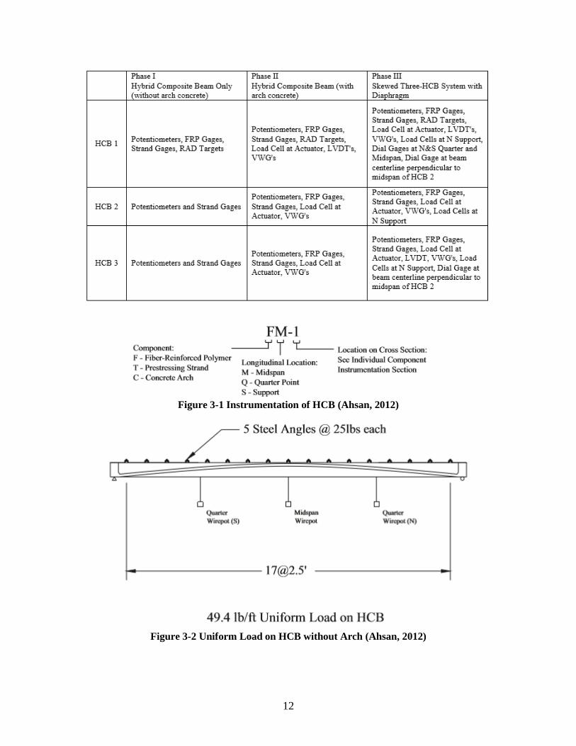
The full HCBs were tested at Virginia Tech after the concrete arch and shear
connectors were placed and 28 days were given for the concrete to cure. This test was
designed to investigate the behavior of the individual HCB. The same layout of strain
gages and pin and roller supports used in this test. Each HCB was tested twice under each
of the two load cases. The first load case was a 15 kips concentrated load at mid-span,
and the second load case was two 12.5 kips concentrated loads (in total 25 kips) at
quarter points (Figure 3-3).
Figure 3-3 Load Cases of Full HCB Tests (Ahsan, 2012)
The three HCB/composite deck system was tested at Virginia Tech after the tests
of the individual HCB. A 7.5 inch thick concrete deck was placed on the top of three
HCBs on a forty-five-degree skew. Two diaphragms were placed at the ends of the three
HCB/composite deck system to alleviate lateral-torsional displacements. A total of 17
tests were performed based on 8 load cases after the concrete achieved adequate strength.
For tests 1-12, a load of four representative tire patches representing the rear axles of a
HL-93 truck was applied on the top of the concrete deck. The tire patches were in 9 in. *
18 in., and they were spaced at 14 feet * 6 feet (Figure 3-35). The load evenly distributed

14
on the four tire patches was 85.12 kips which is the result of the weight of the two rear
axles of a HL-93 truck (64 kips) multiplied by the Dynamic Load Factor 1.33. For the
tests 13-17, a load representing the one wheel line was applied over the centerline of the
deck (Figure 3-4).
Figure 3-4 Load Cases of Three HCB/Composite Deck System Tests (Ahsan, 2012)
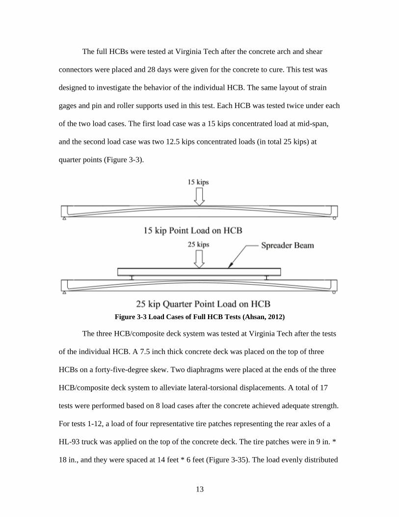
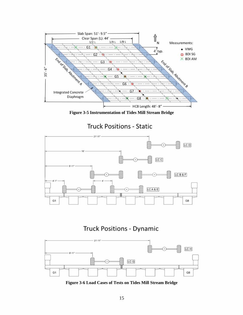
The field testing of the Tides Mill Stream Bridge was conducted by the University
of Virginia. The field testing included three main parts with different instrumentation
plans (Figure 3-5). A static truck load test was performed using exterior strain gages
instrumented on the bridge and internal vibrating wire gages. The truck traversed the
bridge along paths predefined in six load cases at a crawl speed (no impact) and parked at
mid-span for a period of time. Strains were recorded during the entire loading time. A
dynamic truck load test was performed after the static truck load test. . A truck was
driven along paths predefined in two load cases for multiple times. The load cases of
static and dynamic truck load tests is shown in Figure 3-6. Strains were recorded
throughout the testing process. Vibration tests were performed for a set period of time.
Ambient vibrations were recorded by the external accelerometers and the internal
vibrating wire gages. Figure 3-5 and Figure 3-6 come from the field testing plan of the
recent field testing conducted by the University of Virginia.
15
Figure 3-5 Instrumentation of Tides Mill Stream Bridge
Figure 3-6 Load Cases of Tests on Tides Mill Stream Bridge
16
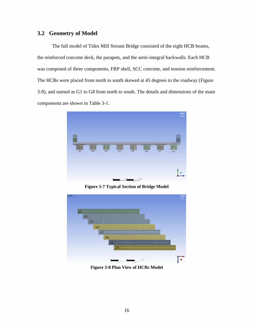
3.2 Geometry of Model
The full model of Tides Mill Stream Bridge consisted of the eight HCB beams,
the reinforced concrete deck, the parapets, and the semi-integral backwalls. Each HCB
was composed of three components, FRP shell, SCC concrete, and tension reinforcement.
The HCBs were placed from north to south skewed at 45 degrees to the roadway (Figure
3-8), and named as G1 to G8 from north to south. The details and dimensions of the main
components are shown in Table 3-1.
Figure 3-7 Typical Section of Bridge Model
Figure 3-8 Plan View of HCBs Model

17
Table 3-1 Dimension of Main Components (Slade & Eriksson, 2012)
Component Dimension Description
Beam
21.33in Height of hybrid composite beam (HCB)
24in Width of HCB shell
34in Length of End Chimney (Must at least the Length of
Bearing Pad)
4in Average Width of Concrete Fin
2 Number of Webs
Shell
0.072in Q64 GFRP laminate thickness
6 Equivalent number of Q64 GFRP layers in the top
flange
1.53 Equivalent number of Q64 GFRP layers in the
bottom flange
1.53 Equivalent number of Q64 GFRP layers in the web
Arch
4in Thickness of arch concrete in HCB
22.5in Width of the Compression Arch Reinforcement
4in Width of "fin" that connects arch to CIP slab
Shear
Reinforcement
5 Stirrup Size for Shear Connectors
45deg Angle of inclination of shear connectors
4in Height of the stirrup above the HCB top flange
Arch
Reinforcement 2
Number of Additional Strands placed in the
compression reinforcing
Slab 7.5in Thickness of CIP slab above HCB
Span 48ft+8in Overall length of section
44ft+4in Design span of section
Bridge
4ft+1in Beam spacing
8 Number of precast sections in bridge cross section
32.5ft Overall width of bridge
30ft Curb to curb width of bridge
15in Width of Barrier
45deg Skew of Bridge
6in Overhang length from CL of Exterior beam
18
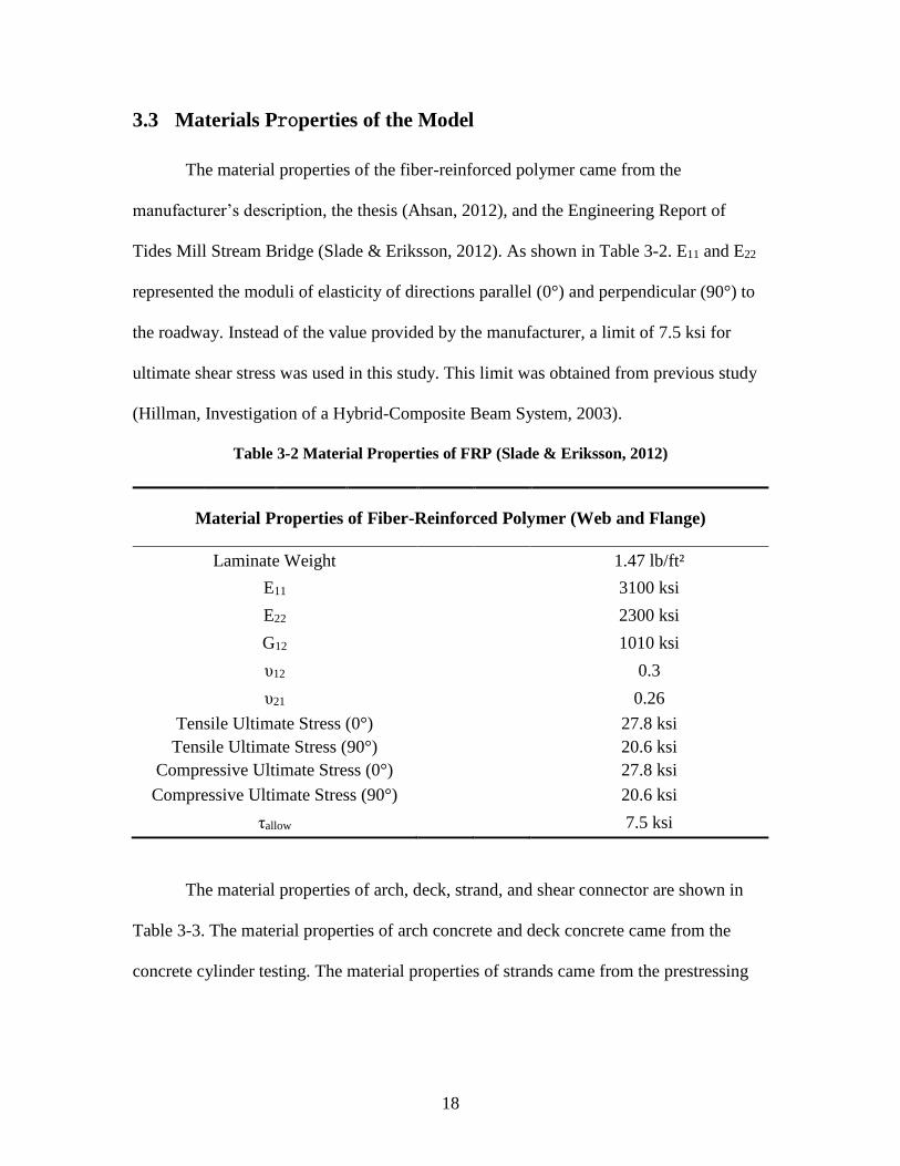
3.3 Materials Properties of the Model
The material properties of the fiber-reinforced polymer came from the
manufacturer’s description, the thesis (Ahsan, 2012), and the Engineering Report of
Tides Mill Stream Bridge (Slade & Eriksson, 2012). As shown in Table 3-2. E11 and E22
represented the moduli of elasticity of directions parallel (0°) and perpendicular (90°) to
the roadway. Instead of the value provided by the manufacturer, a limit of 7.5 ksi for
ultimate shear stress was used in this study. This limit was obtained from previous study
(Hillman, Investigation of a Hybrid-Composite Beam System, 2003).
Table 3-2 Material Properties of FRP (Slade & Eriksson, 2012)
Material Properties of Fiber-Reinforced Polymer (Web and Flange)
Laminate Weight 1.47 lb/ft²
E11 3100 ksi
E22 2300 ksi
G12 1010 ksi
υ12 0.3
υ21 0.26
Tensile Ultimate Stress (0°) 27.8 ksi
Tensile Ultimate Stress (90°) 20.6 ksi
Compressive Ultimate Stress (0°) 27.8 ksi
Compressive Ultimate Stress (90°) 20.6 ksi
τallow 7.5 ksi
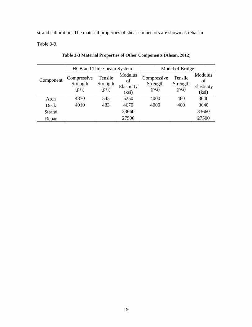
The material properties of arch, deck, strand, and shear connector are shown in
Table 3-3. The material properties of arch concrete and deck concrete came from the
concrete cylinder testing. The material properties of strands came from the prestressing
19
strand calibration. The material properties of shear connectors are shown as rebar in
Table 3-3.
Table 3-3 Material Properties of Other Components (Ahsan, 2012)
Component
HCB and Three-beam System Model of Bridge
Compressive
Strength
(psi)
Tensile
Strength
(psi)
Modulus
of
Elasticity
(ksi)
Compressive
Strength
(psi)
Tensile
Strength
(psi)
Modulus
of
Elasticity
(ksi)
Arch 4870 545 5250 4000 460 3640
Deck 4010 483 4670 4000 460 3640
Strand 33660 33660
Rebar 27500 27500

20
3.4 Model Construction and Analysis
The software used for building and analyzing the models was ANSYS
Workbench 18.1. The computer-aided design (CAD) software was Design Modeler
which is a built-in module of ANSYS Workbench 18.1.
After establishing the models by the built-in CAD tool Design Modeler, the
analysis was commenced in the analytical tool (Mechanical). There were three
components in Mechanical: Model, Static Structural, and Solution. The analysis settings
were included in these sections and will be introduced in each of the three phases.
Three models were developed in this study. Section 3.4.1 and section 3.4.2 focus
on a detailed model of a single HCB beam. Section 3.4.3 includes three HCB beams with
a composite concrete deck. Section 3.4.4 is the development of the full Tides Mill Stream
Bridge.
21
3.4.1 HCB Model without Arch
3.4.1.1 Geometry
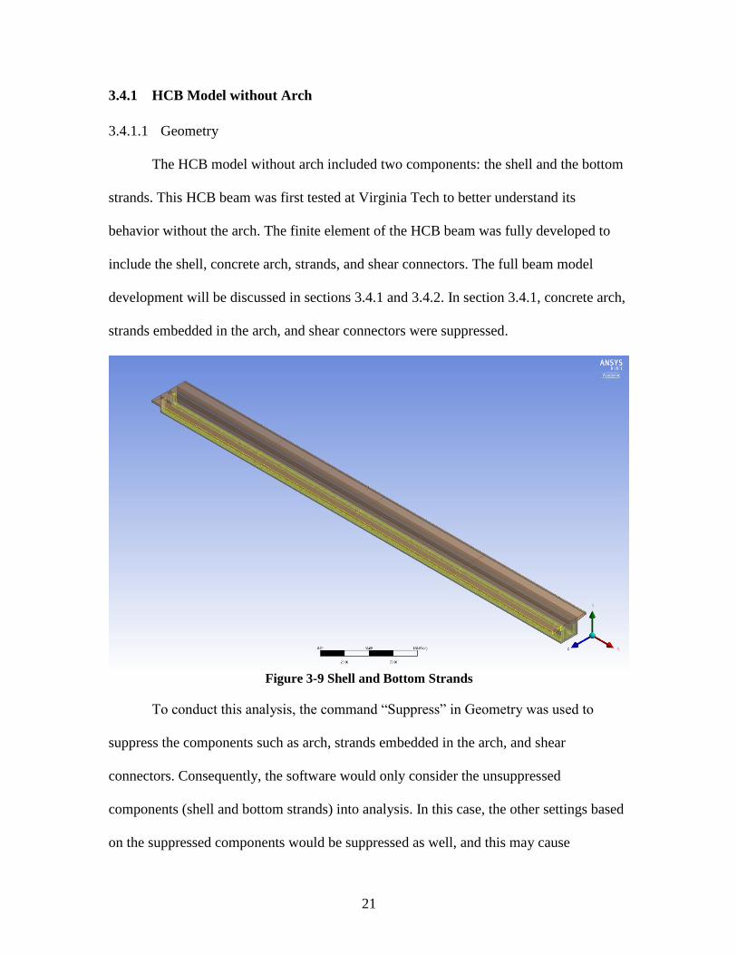
The HCB model without arch included two components: the shell and the bottom
strands. This HCB beam was first tested at Virginia Tech to better understand its
behavior without the arch. The finite element of the HCB beam was fully developed to
include the shell, concrete arch, strands, and shear connectors. The full beam model
development will be discussed in sections 3.4.1 and 3.4.2. In section 3.4.1, concrete arch,
strands embedded in the arch, and shear connectors were suppressed.
Figure 3-9 Shell and Bottom Strands
To conduct this analysis, the command “Suppress” in Geometry was used to
suppress the components such as arch, strands embedded in the arch, and shear
connectors. Consequently, the software would only consider the unsuppressed
components (shell and bottom strands) into analysis. In this case, the other settings based
on the suppressed components would be suppressed as well, and this may cause
22
inaccuracy of the solution. For example, the settings in Construction Geometry,
Coordinate Systems, Connections, and Mesh would be suppressed if the based
geometries were suppressed. Therefore, the construction geometries and coordinate
systems should depend on the components that would not be suppressed through the
analysis process. When performing the analysis of the full HCB, the command
“Unsuppress” was applied on the suppressed components to involve them in the analysis.
Similarly, the suppressed settings were unsuppressed in the meantime.
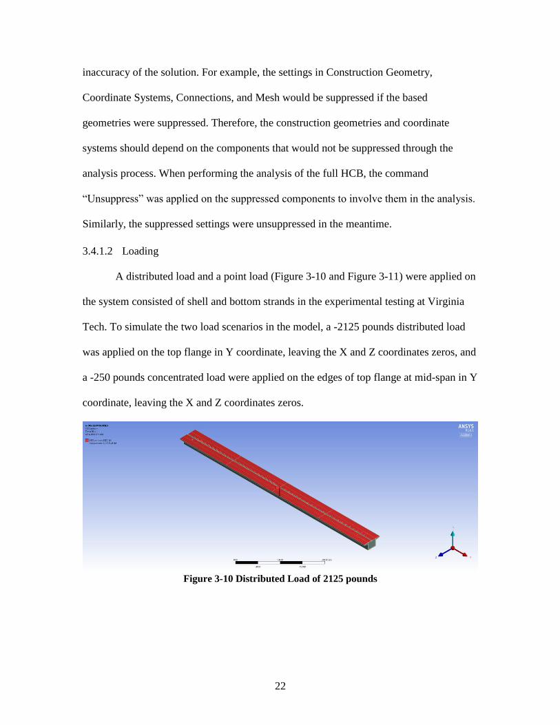
3.4.1.2 Loading
A distributed load and a point load (Figure 3-10 and Figure 3-11) were applied on
the system consisted of shell and bottom strands in the experimental testing at Virginia
Tech. To simulate the two load scenarios in the model, a -2125 pounds distributed load
was applied on the top flange in Y coordinate, leaving the X and Z coordinates zeros, and
a -250 pounds concentrated load were applied on the edges of top flange at mid-span in Y
coordinate, leaving the X and Z coordinates zeros.
Figure 3-10 Distributed Load of 2125 pounds

23
Figure 3-11 Concentrated Load of 250 pounds at Mid-Span

24
3.4.2 Full HCB Model
3.4.2.1 Geometry
The individual HCB beam model (Figure 3-12) included five components:
concrete arch, bottom strands, strands embedded in the arch, shear connectors, and shell.
To accurately simulate the boundary conditions, extra geometries were added to the
model. Considering the purpose of simplification, some assumptions and changes were
made in the model.
Figure 3-12 Model of HCB
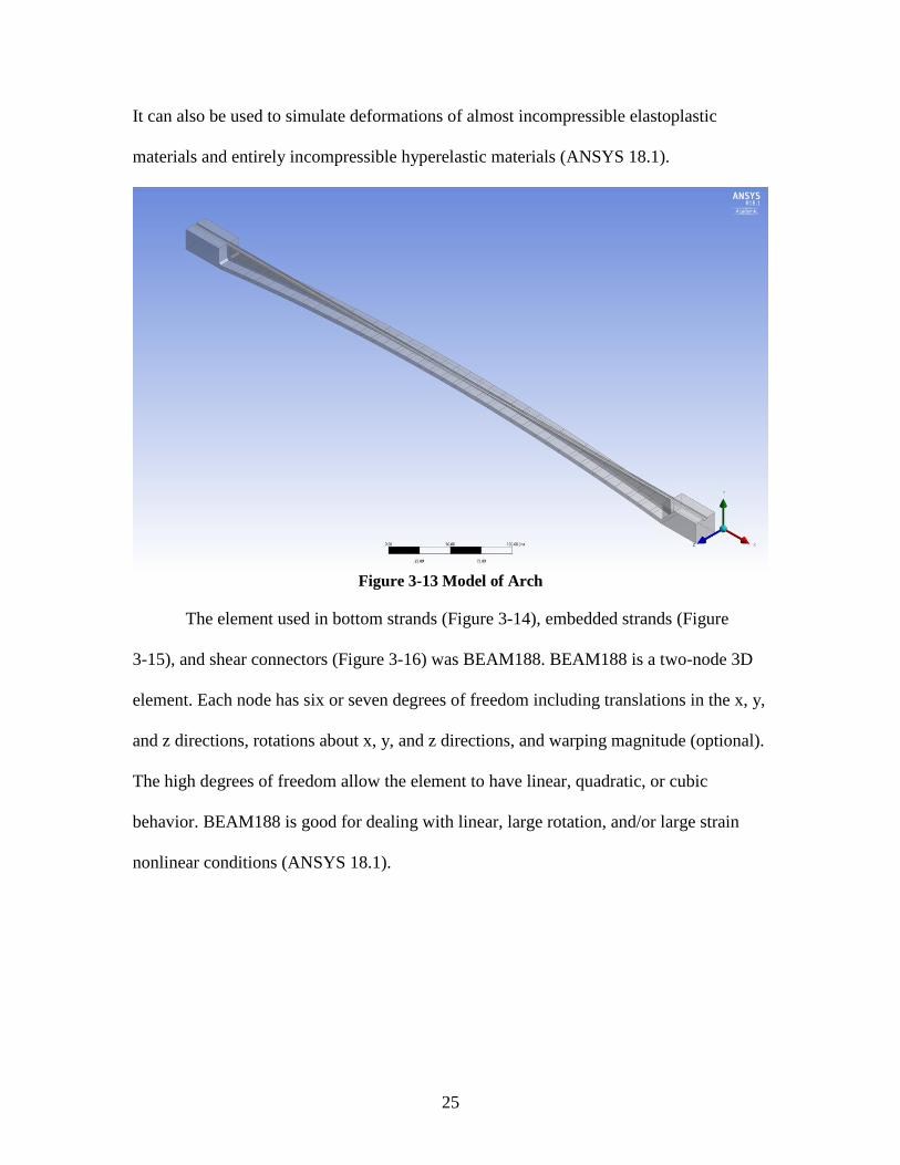
The arch (Figure 3-13) was constructed prior to the other components. The name
of element used in arch was SOLID187. SOLID187, a higher order 3D ANSYS element
including 10 nodes, has quadratic displacement behavior and is able to model irregular
meshes. Each node of the element has three degrees of freedom. SOLID187 is capable to
deal with conditions of plasticity, hyperelasticity, creep, stress stiffening, and large strain.
25
It can also be used to simulate deformations of almost incompressible elastoplastic
materials and entirely incompressible hyperelastic materials (ANSYS 18.1).
Figure 3-13 Model of Arch
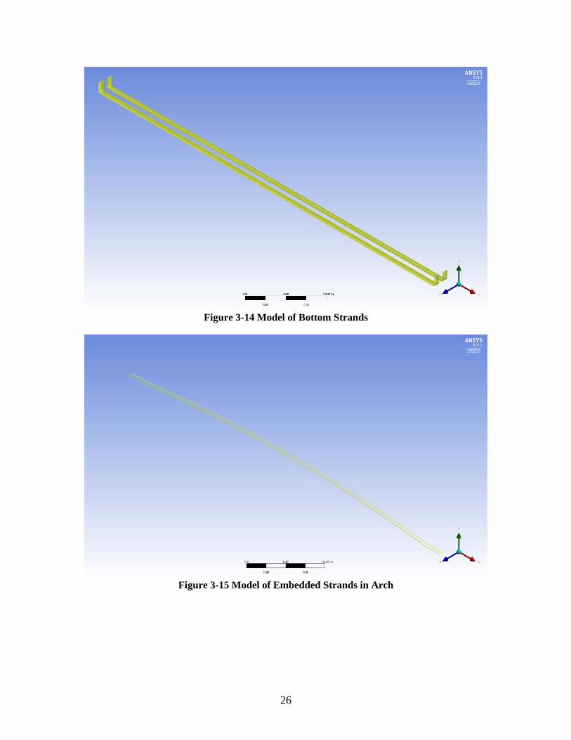
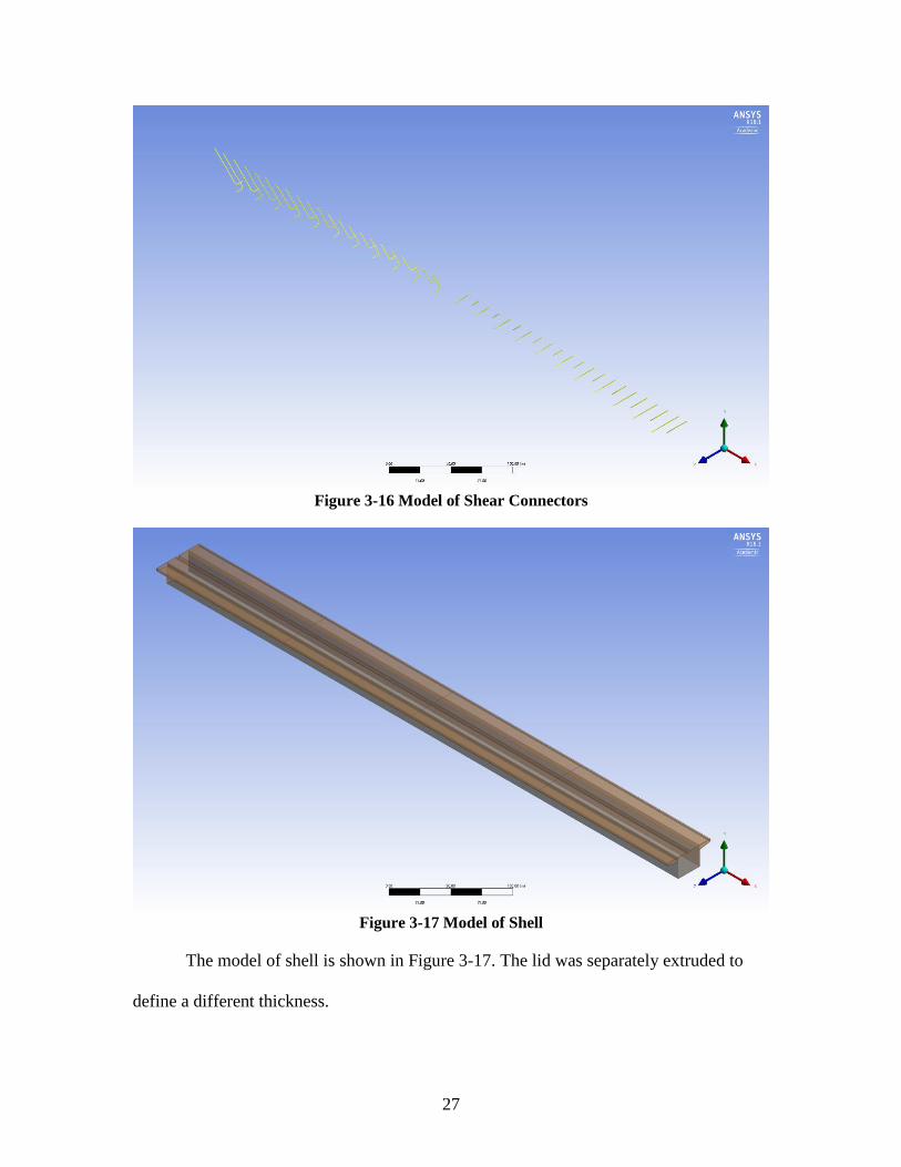
The element used in bottom strands (Figure 3-14), embedded strands (Figure
3-15), and shear connectors (Figure 3-16) was BEAM188. BEAM188 is a two-node 3D
element. Each node has six or seven degrees of freedom including translations in the x, y,
and z directions, rotations about x, y, and z directions, and warping magnitude (optional).
The high degrees of freedom allow the element to have linear, quadratic, or cubic
behavior. BEAM188 is good for dealing with linear, large rotation, and/or large strain
nonlinear conditions (ANSYS 18.1).
26
Figure 3-14 Model of Bottom Strands
Figure 3-15 Model of Embedded Strands in Arch
27
Figure 3-16 Model of Shear Connectors
Figure 3-17 Model of Shell
The model of shell is shown in Figure 3-17. The lid was separately extruded to
define a different thickness.
28
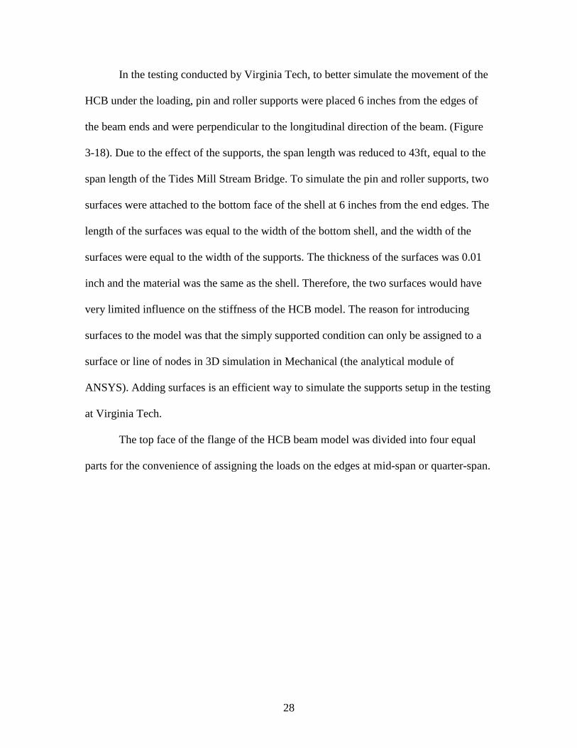
In the testing conducted by Virginia Tech, to better simulate the movement of the
HCB under the loading, pin and roller supports were placed 6 inches from the edges of
the beam ends and were perpendicular to the longitudinal direction of the beam. (Figure
3-18). Due to the effect of the supports, the span length was reduced to 43ft, equal to the
span length of the Tides Mill Stream Bridge. To simulate the pin and roller supports, two
surfaces were attached to the bottom face of the shell at 6 inches from the end edges. The
length of the surfaces was equal to the width of the bottom shell, and the width of the
surfaces were equal to the width of the supports. The thickness of the surfaces was 0.01
inch and the material was the same as the shell. Therefore, the two surfaces would have
very limited influence on the stiffness of the HCB model. The reason for introducing
surfaces to the model was that the simply supported condition can only be assigned to a
surface or line of nodes in 3D simulation in Mechanical (the analytical module of
ANSYS). Adding surfaces is an efficient way to simulate the supports setup in the testing
at Virginia Tech.
The top face of the flange of the HCB beam model was divided into four equal
parts for the convenience of assigning the loads on the edges at mid-span or quarter-span.
29
Figure 3-18 Model of Added Surface
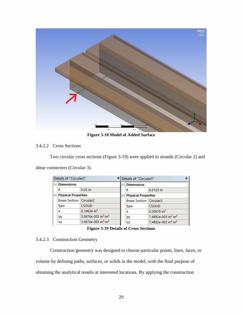
3.4.2.2 Cross Sections
Two circular cross sections (Figure 3-19) were applied to strands (Circular 2) and
shear connecters (Circular 3).
Figure 3-19 Details of Cross Sections
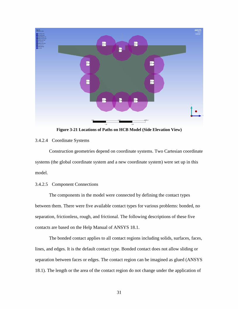
3.4.2.3 Construction Geometry
Construction geometry was designed to choose particular points, lines, faces, or
volume by defining paths, surfaces, or solids in the model, with the final purpose of
obtaining the analytical results at interested locations. By applying the construction

30
geometries, the user is able to screen and obtain the results of interested nodes accurately
and rapidly. The model of HCB consisted of ten paths, corresponding to the locations of
the gauges in the testing at Virginia Tech. The detailed locations are shown in Table 3-4,
Figure 3-20, and Figure 3-21.
Table 3-4 Paths of HCB Model
Path Location Start End
1 Top Flange East North South
2 Top Flange West North South
3 Top Web East North South
4 Top Web West North South
5 Bottom Web East North South
6 Bottom Web West North South
7 Bottom Flange East North South
8 Bottom Flange West North South
9 Top Arch North South
10 Bottom Flange North South
Figure 3-20 Plan View of Paths on HCB Model
31
Figure 3-21 Locations of Paths on HCB Model (Side Elevation View)
3.4.2.4 Coordinate Systems
Construction geometries depend on coordinate systems. Two Cartesian coordinate
systems (the global coordinate system and a new coordinate system) were set up in this
model.
3.4.2.5 Component Connections
The components in the model were connected by defining the contact types
between them. There were five available contact types for various problems: bonded, no
separation, frictionless, rough, and frictional. The following descriptions of these five
contacts are based on the Help Manual of ANSYS 18.1.
The bonded contact applies to all contact regions including solids, surfaces, faces,
lines, and edges. It is the default contact type. Bonded contact does not allow sliding or
separation between faces or edges. The contact region can be imagined as glued (ANSYS
18.1). The length or the area of the contact region do not change under the application of

32
the load, so bonded contact allows for a linear solution. In the calculation of
mathematical model, any gaps between contact bodies will be closed automatically, and
any initial penetration will be disregarded. In this model, most of the type of contact
regions were defined as bonded.
The no separation contact applies to faces between 3D solids or edges on 2D
plates. It does not allow separation between the geometries in contact.
The frictionless contact allows a gap to exist between geometries depending on
the applied load. When the separation occurs, the normal pressure equals to zero. Free
sliding is allowed in this type of contact, because the coefficient of friction is assumed as
zero.
The rough contact prevents sliding from happening between the contact
geometries. It only applies to faces of solids in 3D simulations or edges of plates in 2D
simulations. For this contact type, the gaps between contact geometries will not be closed
automatically.
The frictional contact allows the contact geometries keep a no sliding status
before the shear stress between the two contact geometries exceeds a certain value which
can be defined by users. Once this defined shear stress is exceeded, the contact
geometries are allowed to have relative sliding.
3.4.2.6 Contact Conditions
Six contact conditions were used in the finite element model development and
will be introduced in this section. The connection between the shell and the arch was
defined as no separation, because the connection between them was weak, according to
33
the experimental testing at Virginia Tech. This will be discussed further in Chapter Four
(section 4.2.1).
The contact type between the top flange and deck was originally defined as
bonded in section 3.4.3. This contact type was later modified to reflect better
comparisons to the experimental results and will be further discussed in Chapter Four
(section 4.2.1).
The bottom strands were connected to the shell by infusing vinyl-ester into the
mold where strands had been placed prior to the infusion. According to the experimental
testing at Virginia Tech, the strain of bottom shell at mid-span was 812 με, while the
average strain of bottom strands at mid-span was 740 με. The small difference of 72 με
shown that composite condition of bottom shell and bottom strands was strong.
Therefore, the contact condition was defined as bonded.
The main function of strands embedded in arch was anchoring the shear
connectors. They were fabricated into the concrete arch, and it assumed no relative
sliding occurred. Hence, the contact type between them was defined as bonded.
The function of the shear connectors was to insure composite action between the
HCBs and the bridge deck. The lower parts were embedded into the concrete arch, and
attached to the embedded strands. There was no sliding allowed between the shear
connectors and the concrete arch. Hence, the contact type between them was defined as
bonded.
As described in section 3.4.2.10, the bottom shell was separated from the whole
shell to allow adjustment of its material property. Ultimately, these two parts were
integrated in the beam, acting as a whole shell. Sliding and separation were not allowed
34
between them. Hence, the contact type between the shell and bottom shell in the model
was defined as bonded.
The surfaces were designed for defining the supports. The supports were applied
on the surfaces, and the surfaces were bonded to the bottom face of the shell.
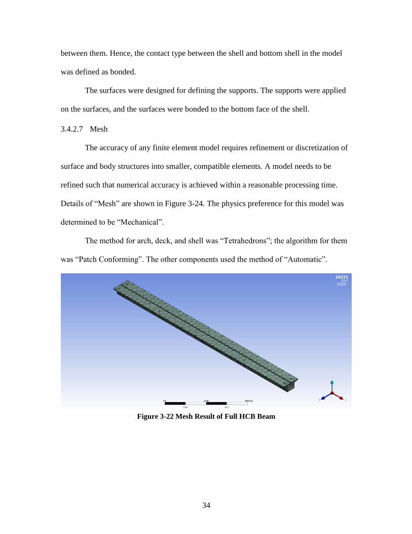
3.4.2.7 Mesh
The accuracy of any finite element model requires refinement or discretization of
surface and body structures into smaller, compatible elements. A model needs to be
refined such that numerical accuracy is achieved within a reasonable processing time.
Details of “Mesh” are shown in Figure 3-24. The physics preference for this model was
determined to be “Mechanical”.
The method for arch, deck, and shell was “Tetrahedrons”; the algorithm for them
was “Patch Conforming”. The other components used the method of “Automatic”.
Figure 3-22 Mesh Result of Full HCB Beam

35
Figure 3-23 Details of “Patch Conforming Method”
Figure 3-24 Details of “Mesh”

36
3.4.2.8 Supports
A simply supported support and a displacement support were used to simulate the
pin and roller in the Virginia Tech’s test. The following descriptions of the supports were
based on the Help Manual of ANSYS 18.1.
The moving or deforming of straight and curved edges or vertices are constrained
by simply supported boundary condition. However, rotations are free. (ANSYS 18.1).
Simply supported boundary condition can only be applied on surface and line body.
When simply supported boundary condition is required on a solid body, forming a
surface or a line body to simulate the boundary condition is a reasonable methodology. In
the model of HCB, a simply supported condition was assigned on the added surface at
one end of the bottom flange.
A displacement boundary condition (commonly referred as a roller support)
allows body, including flat or curved faces or edges or vertices, to displace from their
original locations to new locations by defining the three components of a displacement
vector based on the world coordinate system or local coordinate systems (ANSYS 18.1).
It is supported by geometries for solid, surface/shell, and wire body/line body/beam. In
this model, a displacement boundary condition was assigned on the surface at the other
end of the bottom flange.
3.4.2.9 Loading
Two point loads (Figure 3-25 and Figure 3-26) were applied on the full HCB in
the experimental testing at Virginia Tech. To simulate the two load scenarios in the
model of HCB, a 15 kips load was assigned on the edges of top flange at mid-span in Y
coordinate, leaving the X and Z coordinates zeros, and a 25 kips load was applied on the
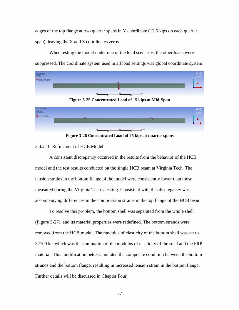
37
edges of the top flange at two quarter spans in Y coordinate (12.5 kips on each quarter
span), leaving the X and Z coordinates zeros.
When testing the model under one of the load scenarios, the other loads were
suppressed. The coordinate system used in all load settings was global coordinate system.
Figure 3-25 Concentrated Load of 15 kips at Mid-Span
Figure 3-26 Concentrated Load of 25 kips at quarter spans
3.4.2.10 Refinement of HCB Model
A consistent discrepancy occurred in the results from the behavior of the HCB
model and the test results conducted on the single HCB beam at Virginia Tech. The
tension strains in the bottom flange of the model were consistently lower than those
measured during the Virginia Tech’s testing. Consistent with this discrepancy was
accompanying differences in the compression strains in the top flange of the HCB beam.
To resolve this problem, the bottom shell was separated from the whole shell
(Figure 3-27), and its material properties were redefined. The bottom strands were
removed from the HCB model. The modulus of elasticity of the bottom shell was set to
32100 ksi which was the summation of the modulus of elasticity of the steel and the FRP
material. This modification better simulated the composite condition between the bottom
strands and the bottom flange, resulting in increased tension strain in the bottom flange.
Further details will be discussed in Chapter Four.

38
Figure 3-27 Separated Bottom Shell
39
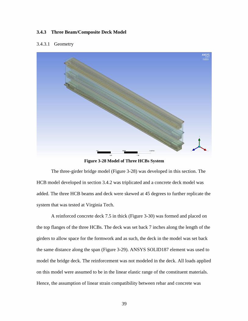
3.4.3 Three Beam/Composite Deck Model
3.4.3.1 Geometry
Figure 3-28 Model of Three HCBs System
The three-girder bridge model (Figure 3-28) was developed in this section. The
HCB model developed in section 3.4.2 was triplicated and a concrete deck model was
added. The three HCB beams and deck were skewed at 45 degrees to further replicate the
system that was tested at Virginia Tech.
A reinforced concrete deck 7.5 in thick (Figure 3-30) was formed and placed on
the top flanges of the three HCBs. The deck was set back 7 inches along the length of the
girders to allow space for the formwork and as such, the deck in the model was set back
the same distance along the span (Figure 3-29). ANSYS SOLID187 element was used to
model the bridge deck. The reinforcement was not modeled in the deck. All loads applied
on this model were assumed to be in the linear elastic range of the constituent materials.
Hence, the assumption of linear strain compatibility between rebar and concrete was
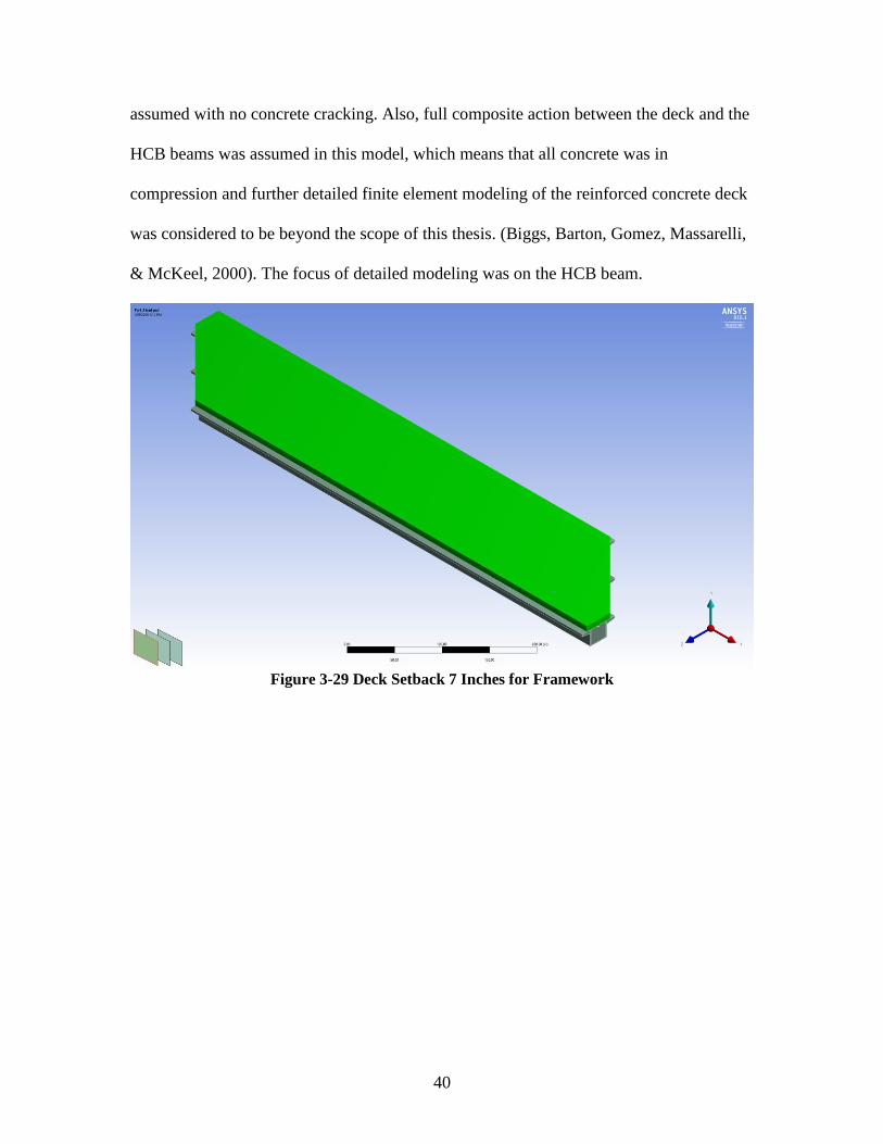
40
assumed with no concrete cracking. Also, full composite action between the deck and the
HCB beams was assumed in this model, which means that all concrete was in
compression and further detailed finite element modeling of the reinforced concrete deck
was considered to be beyond the scope of this thesis. (Biggs, Barton, Gomez, Massarelli,
& McKeel, 2000). The focus of detailed modeling was on the HCB beam.
Figure 3-29 Deck Setback 7 Inches for Framework

41
Figure 3-30 Model of Deck on Three HCBs
In the experimental testing at Virginia Tech, a total of seventeen tests were
conducted based on eight load configurations simulating eight locations of a HL-93 truck
on the deck. The truck’s load was transferred through four representative tire footprints (9
inches by 18 inches) to the deck. Four footprints represent the load of a truck, and were
arranged at 6 feet transversely and 14 feet longitudinally. To simulate the eight load
configurations, a total of twenty-eight surfaces (Figure 3-31) were attached to the top face
of the deck. These surfaces followed the size and the locations of the tire footprints in the
eight load configurations. To make less influence to the stiffness of the model, the
thickness of the surfaces was defined as 0.01 inch and the material was the same as that
of the deck.
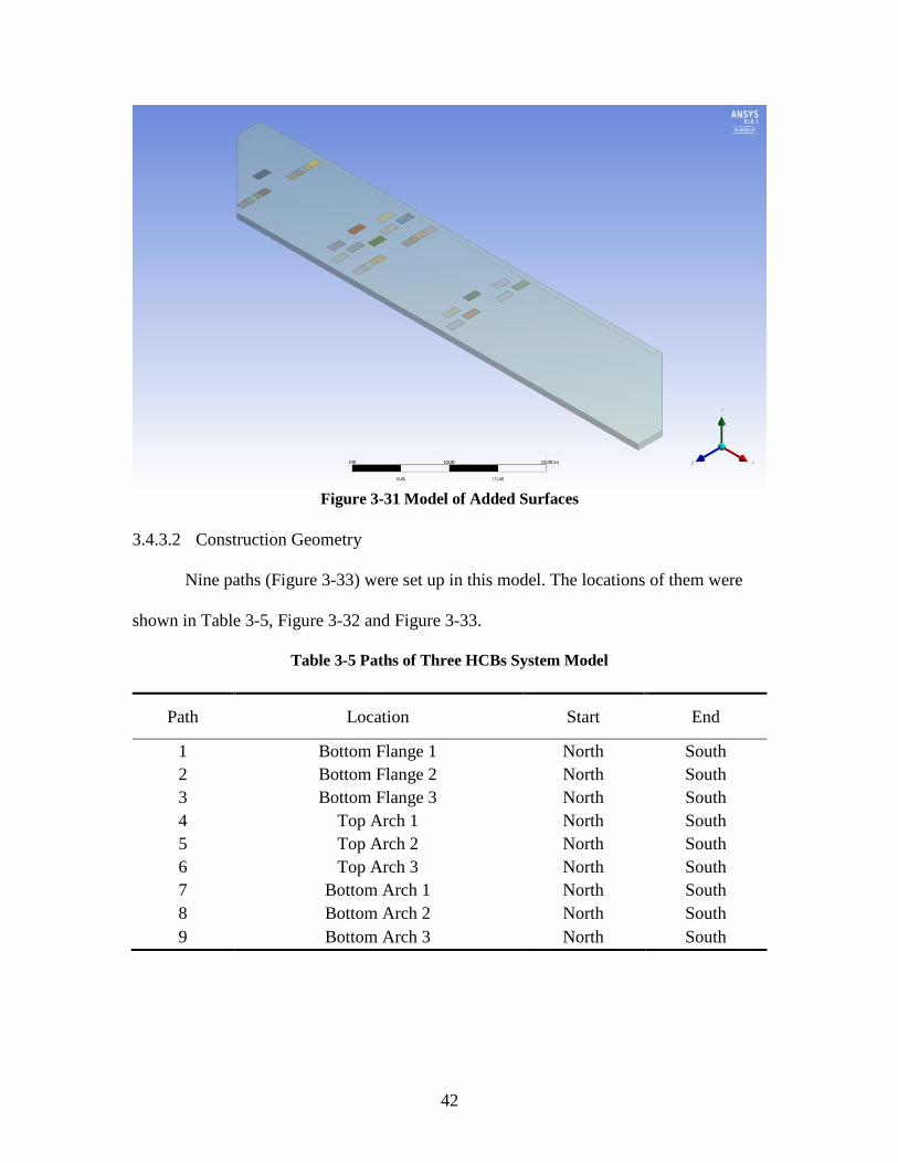
42
Figure 3-31 Model of Added Surfaces
3.4.3.2 Construction Geometry
Nine paths (Figure 3-33) were set up in this model. The locations of them were
shown in Table 3-5, Figure 3-32 and Figure 3-33.
Table 3-5 Paths of Three HCBs System Model
Path Location Start End
1 Bottom Flange 1 North South
2 Bottom Flange 2 North South
3 Bottom Flange 3 North South
4 Top Arch 1 North South
5 Top Arch 2 North South
6 Top Arch 3 North South
7 Bottom Arch 1 North South
8 Bottom Arch 2 North South
9 Bottom Arch 3 North South

43
Figure 3-32 Locations of Paths on Three HCBs System Model (Side Elevation View)
Figure 3-33 Paths of Three HCBs System Model
3.4.3.3 Connections
Shear connectors were used to insure composite action between the deck and
HCB beams. The shear connectors were tightly aligned and were anchored into both the
arch and the deck, which insured none or very limited separation or relative sliding would
occur between the deck and HCBs. Therefore, the contact type between the deck and
three shells was bonded. The contact type between the deck and shear connectors was
also bonded.

44
3.4.3.4 Supports
In Virginia Tech’s testing, pin supports and roller supports were used, similar to
the testing of the single HCB beam tests. Therefore, simply supported supports and
displacement supports were set up on each of the three HCB models, the configuration
followed that used in section 3.4.2.
In Virginia Tech’s testing, diaphragms were placed at the ends of beams to
prevent the beams from lateral translations and rotations about the global X-axis. In this
model, the function of the diaphragms was achieved by restraining the beams from
moving in the global Z axis and rotating about the global X axis.

45
3.4.3.5 Loads
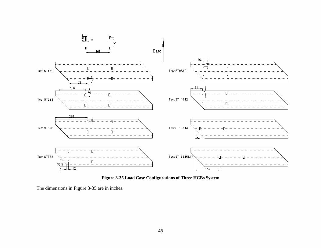
There were seventeen tests based on eight load cases in Virginia Tech’s testing.
The first six load cases simulated a load of 85.12 kips (85 kips in testing), which is the
combined two rear axle loads (32 kips/axle) of a HL-93 truck (64 kips) multiplied by the
Dynamic Load Factor of 1.33. The last two load cases simulated the condition that only
two wheels from the same side were on the deck, and the load was reduced to 43 kips.
Each red rectangle in Figure 3-34 represented a footprint of the truck. The loads were
evenly distributed on all the footprints. The configurations of load cases were shown in
Figure 3-35.
Figure 3-34 Eight Load Cases of Three HCBs System Model
46
Figure 3-35 Load Case Configurations of Three HCBs System
The dimensions in Figure 3-35 are in inches.
47
3.4.4 Model of Tides Mill Stream Bridge
3.4.4.1 Geometry
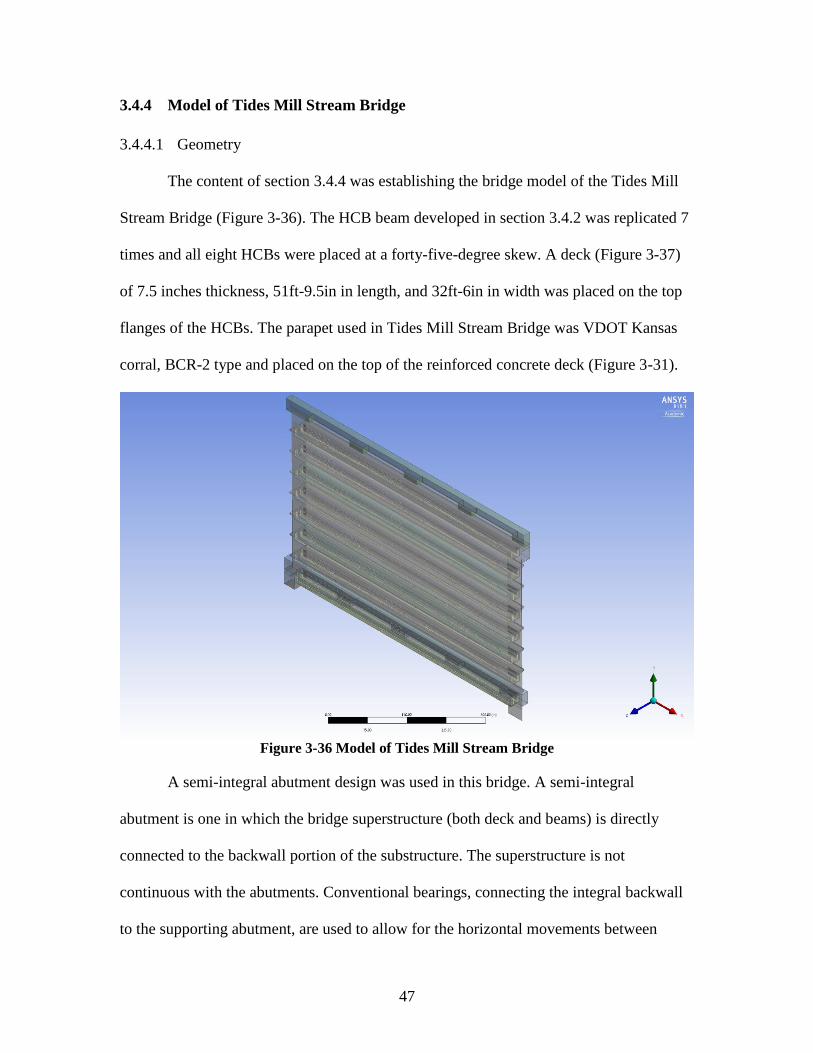
The content of section 3.4.4 was establishing the bridge model of the Tides Mill
Stream Bridge (Figure 3-36). The HCB beam developed in section 3.4.2 was replicated 7
times and all eight HCBs were placed at a forty-five-degree skew. A deck (Figure 3-37)
of 7.5 inches thickness, 51ft-9.5in in length, and 32ft-6in in width was placed on the top
flanges of the HCBs. The parapet used in Tides Mill Stream Bridge was VDOT Kansas
corral, BCR-2 type and placed on the top of the reinforced concrete deck (Figure 3-31).
Figure 3-36 Model of Tides Mill Stream Bridge
A semi-integral abutment design was used in this bridge. A semi-integral
abutment is one in which the bridge superstructure (both deck and beams) is directly
connected to the backwall portion of the substructure. The superstructure is not
continuous with the abutments. Conventional bearings, connecting the integral backwall
to the supporting abutment, are used to allow for the horizontal movements between

48
superstructure and abutment. The advantage of semi-integral bridges is the removal of
expansion joints at the ends of the bridge, thus alleviating a maintenance issue. The
flexural rigidity of the imbedded beams is influenced by the torsional stiffness of the
backwall structure. In order to simulate this behavior, the eight HCBs were embedded
into the backwalls at both ends of the bridge. The model of backwalls is shown in Figure
3-39 and Figure 3-40.
SOLID187 elements were used in the deck, the parapets, and the backwalls.
Figure 3-37 Model of Bridge Deck

49
Figure 3-38 Model of Bridge Parapets
Figure 3-39 Model of Bridge Backwalls

50
Figure 3-40 Illustration of HCB Beam (G5) Embedded into Backwalls
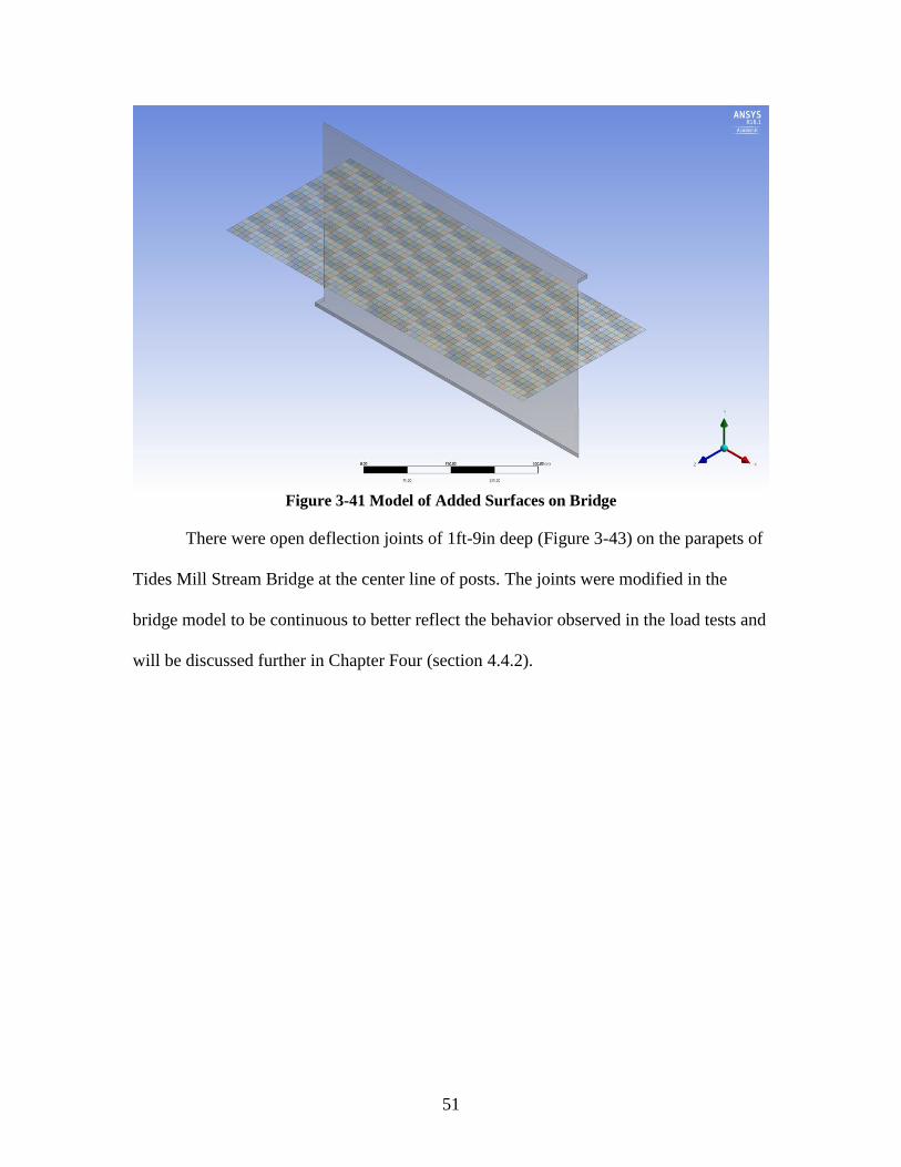
To accurately apply the loads to the deck, a series of surfaces (Figure 3-41) were
introduced on the top face of the bridge deck. Again, the thickness of the surface was
defined as 0.01 in, and the material was identical to the deck. In the field testing
conducted by the University of Virginia, the tire footprints of the two trucks were
13inches by 10inches (130 square inches’ area) and 13inches by 11inches (143 square
inches’ area). To simulate the loads of the trucks and simplify the model at the same time,
the whole surface was divided to 1500 squares with size 12 inches by 12 inches (142
square inches’ area). There were six load configurations of the testing. The detailed
configurations were shown in Figure 3-48 and Figure 3-49. The surface can be cut into
even smaller squares to achieve additional accuracy.
51
Figure 3-41 Model of Added Surfaces on Bridge
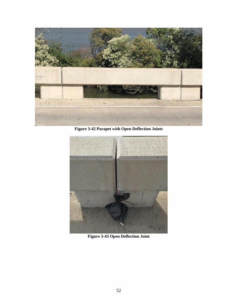
There were open deflection joints of 1ft-9in deep (Figure 3-43) on the parapets of
Tides Mill Stream Bridge at the center line of posts. The joints were modified in the
bridge model to be continuous to better reflect the behavior observed in the load tests and
will be discussed further in Chapter Four (section 4.4.2).
52
Figure 3-42 Parapet with Open Deflection Joints
Figure 3-43 Open Deflection Joint
53
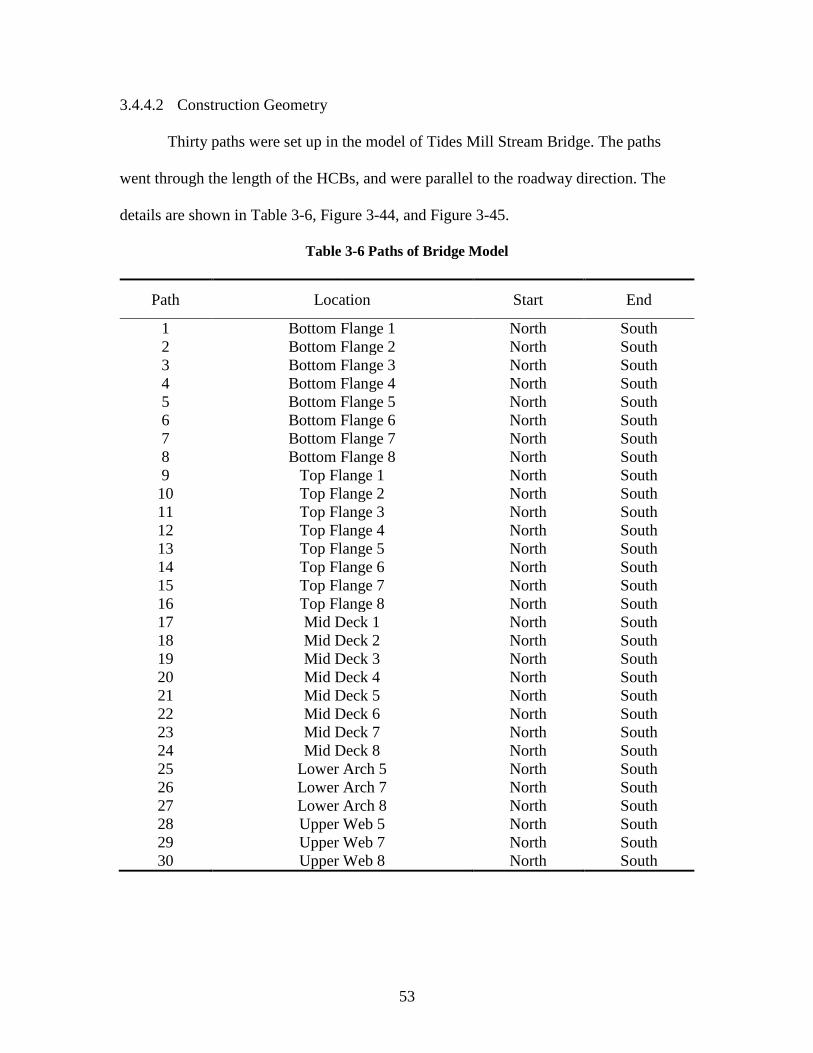
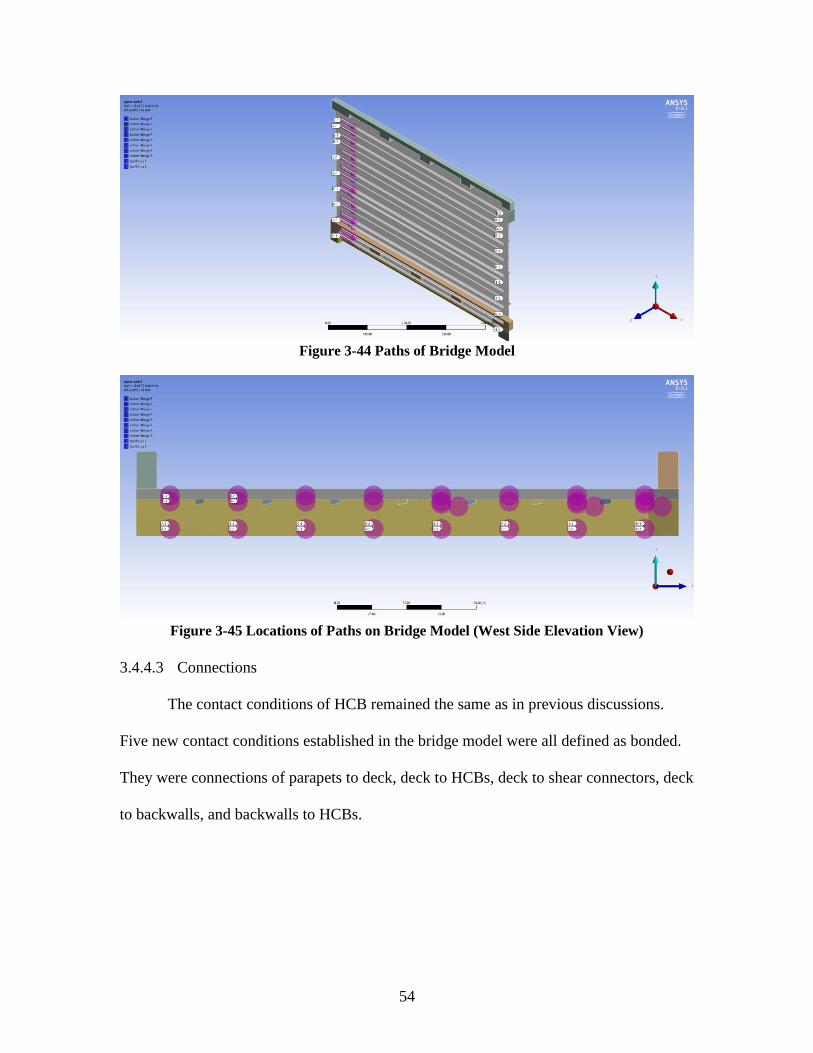
3.4.4.2 Construction Geometry
Thirty paths were set up in the model of Tides Mill Stream Bridge. The paths
went through the length of the HCBs, and were parallel to the roadway direction. The
details are shown in Table 3-6, Figure 3-44, and Figure 3-45.
Table 3-6 Paths of Bridge Model
Path Location Start End
1 Bottom Flange 1 North South
2 Bottom Flange 2 North South
3 Bottom Flange 3 North South
4 Bottom Flange 4 North South
5 Bottom Flange 5 North South
6 Bottom Flange 6 North South
7 Bottom Flange 7 North South
8 Bottom Flange 8 North South
9 Top Flange 1 North South
10 Top Flange 2 North South
11 Top Flange 3 North South
12 Top Flange 4 North South
13 Top Flange 5 North South
14 Top Flange 6 North South
15 Top Flange 7 North South
16 Top Flange 8 North South
17 Mid Deck 1 North South
18 Mid Deck 2 North South
19 Mid Deck 3 North South
20 Mid Deck 4 North South
21 Mid Deck 5 North South
22 Mid Deck 6 North South
23 Mid Deck 7 North South
24 Mid Deck 8 North South
25 Lower Arch 5 North South
26 Lower Arch 7 North South
27 Lower Arch 8 North South
28 Upper Web 5 North South
29 Upper Web 7 North South
30 Upper Web 8 North South
54
Figure 3-44 Paths of Bridge Model
Figure 3-45 Locations of Paths on Bridge Model (West Side Elevation View)
3.4.4.3 Connections
The contact conditions of HCB remained the same as in previous discussions.
Five new contact conditions established in the bridge model were all defined as bonded.
They were connections of parapets to deck, deck to HCBs, deck to shear connectors, deck
to backwalls, and backwalls to HCBs.

55
3.4.4.4 Supports
In this model, a simple support was assigned on the inward longitudinal edge of
the bottom surface on the western backwall (Figure 3-46), and a displacement support
was assigned on the inward longitudinal edge of the bottom face on the eastern backwall
(Figure 3-47). The eastern backwall was defined as free in the X direction (the
longitudinal direction of the span). All supports were fixed in the Y and Z directions.
Figure 3-46 Simply Supported Support at Western Backwall (Bottom View)
Figure 3-47 Displacement Support at Eastern Backwall (Bottom View)
56
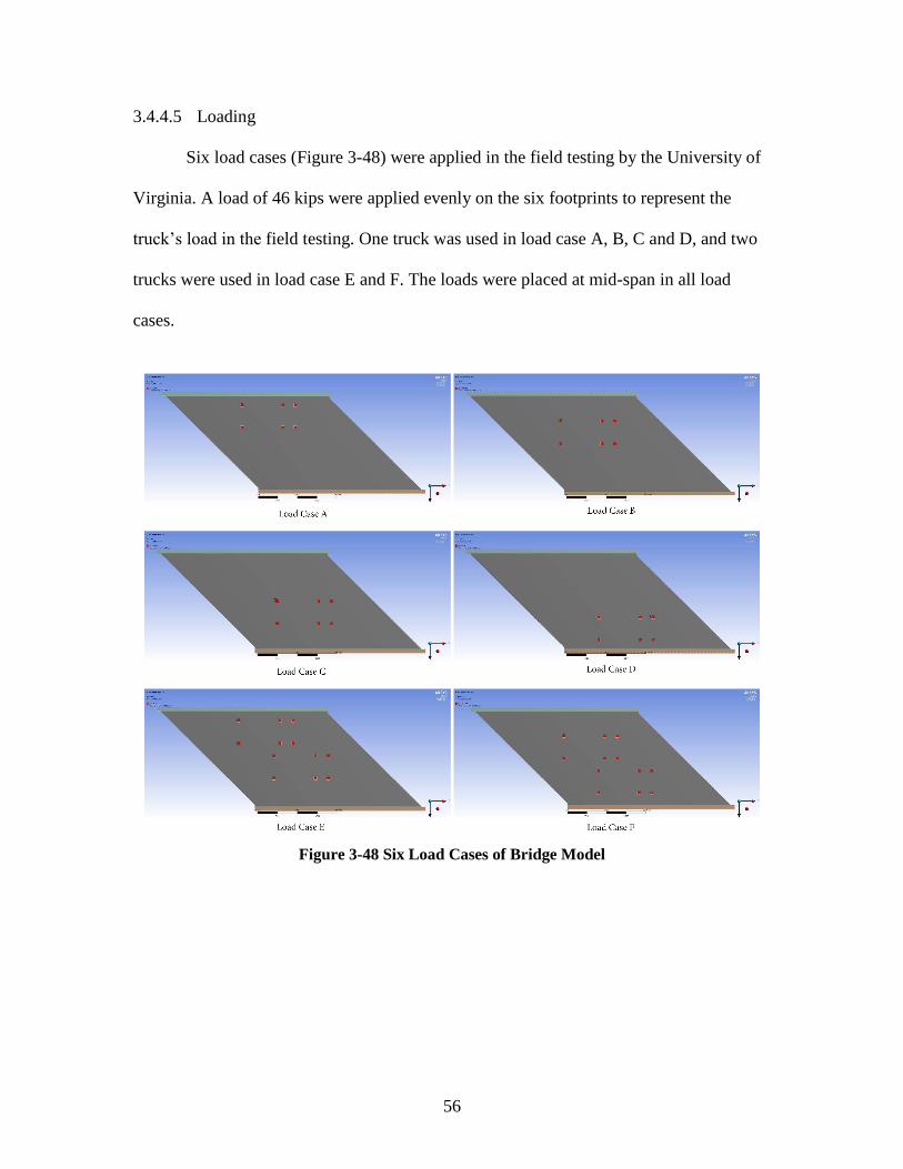
3.4.4.5 Loading
Six load cases (Figure 3-48) were applied in the field testing by the University of
Virginia. A load of 46 kips were applied evenly on the six footprints to represent the
truck’s load in the field testing. One truck was used in load case A, B, C and D, and two
trucks were used in load case E and F. The loads were placed at mid-span in all load
cases.
Figure 3-48 Six Load Cases of Bridge Model

57
Figure 3-49 Load Case Configurations of Tides Mill Stream Bridge

58
3.4.4.6 Refinement of Semi-Integral Backwalls
The semi-integral backwalls significantly influenced the performance the bridge
model, especially the performance of the girders at the two sides (girder G1 and G8). The
configuration of the semi-integral backwalls was introduced in section 3.4.4.1. This will
be discussed further in Chapter Four (section 4.4.3).

59
4 Results and Discussion
The results from the three models of this study were compared with the results
from the thesis of Virginia Tech’s student Ahsan (2012) and the results from the field
testing by the University of Virginia. All results were collected from the modified model
as discussed in section 3.4.2.10 and section 4.2.2 (material of bottom shell was redefined
and bottom strands were removed).
The results from models of this study were labeled as “Model” in tables and
figures. Similarly, the results from the experimental testing at Virginia Tech and the
University of Virginia were labeled as “VT” and “UVA” in tables and figures.
4.1 HCB Model without Arch
In the testing at Virginia Tech, eight tests were conducted on three HCBs. For
HCB 2 and HCB 3, two distributed load tests and a concentrated load test were
conducted. For HCB 1, one distributed load test and one concentrated load test were
conducted.
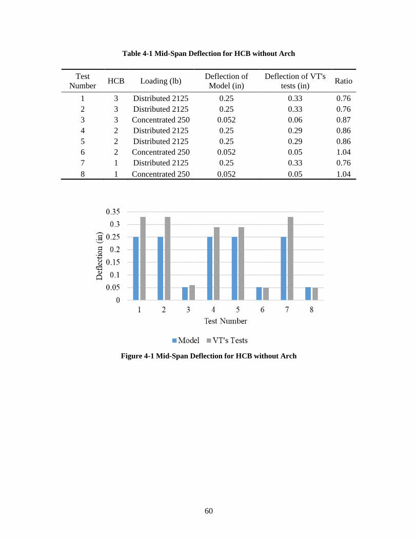
The comparison of mid-span deflections for HCB model without the concrete
arch is shown in Table 4-1 and Figure 4-1. The deflections of the model under distributed
loads were generally smaller than those of the Virginia Tech tests. The deflections of the
model under concentrated loads were closer to the test results.
60
Table 4-1 Mid-Span Deflection for HCB without Arch
Test
Number HCB Loading (lb)
Deflection of
Model (in)
Deflection of VT's
tests (in) Ratio
1 3 Distributed 2125 0.25 0.33 0.76
2 3 Distributed 2125 0.25 0.33 0.76
3 3 Concentrated 250 0.052 0.06 0.87
4 2 Distributed 2125 0.25 0.29 0.86
5 2 Distributed 2125 0.25 0.29 0.86
6 2 Concentrated 250 0.052 0.05 1.04
7 1 Distributed 2125 0.25 0.33 0.76
8 1 Concentrated 250 0.052 0.05 1.04
Figure 4-1 Mid-Span Deflection for HCB without Arch

61
The comparison of mid-span strains for test 7 are shown in Table 4-2 and Figure
4-2. Test 7 was performed on HCB 1 under a uniformly distributed load of 2125 lb/ft.
Table 4-2 Mid-Span Strains for Tests 7 (HCB without Arch)
Location Strain (µƐ)
Ratio Model VT's Test
Top Flange E. -76.27 -136.00 0.56
Top Flange W. -76.50 -89.00 0.86
Top of Web E. -25.65 -40.00 0.64
Top of Web W. -23.68 -81.00 0.29
Bottom Web E. 19.92 0.00 0.00
Bottom Web W. 24.22 -5.00 -4.84
Bottom Flange E. 65.75 81.00 0.81
Bottom Flange W. 65.14 71.00 0.92
Figure 4-2 Mid-Span Strains for Tests 7 (HCB without Arch)

62
The comparison of quarter point strains for test 7 are shown in Table 4-3 and
Figure 4-3. The top flange and top web compressed not as much as those parts in the real
shell.
Table 4-3 Quarter Strains for Tests 7 (HCB without Arch)
Location Strain (µƐ)
Ratio Model VT's Test
Top Flange E. -56.93 -146 0.39
Top Flange W. -55.81 -116 0.48
Top of Web E. -17.514 -77 0.23
Top of Web W. -18.636 -91 0.20
Bottom Web E. 15.972 23 0.69
Bottom Web W. 14.673 11 1.33
Bottom Flange E. 48.67 -26 -1.87
Bottom Flange W. 48.757 36 1.35
Figure 4-3 Quarter Strains for Tests 7 (HCB without Arch)
There were discrepancies of the magnitudes of strains between the results from
the model and the Virginia Tech’s testing. The strain profiles were basically correct, and
the location of the natural axes were close. The focus was on the behavior of the full
HCB model and the three beam/composite deck model.

63
4.2 Full HCB Model
4.2.1 Discussion about Contact Conditions
As mentioned in section 3.4.2.6, the contact type between the shell and the arch
was defined as no separation because the connection between them was weak. According
to the results from Virginia Tech’s test, the strain at the top shell at mid-span was -530
με, while the strain of the top arch at mid-span was only -164 με. The significant
difference between these two contact regions indicated the composite condition between
them was weak. Thus, the appropriate contact type should be a condition between no-
separation and bonded. Similarly, the contact type between the top flange and deck was
defined as bonded, even the real contact condition between them should be a contact type
between no-separation and bonded. By defining the contact type between the top shell
and the arch as no-separation and defining the contact type between the top shell and the
deck as bonded, the model of the bridge was better able to simulate the performance of
the bridge. Hence, these contact types were kept in use.
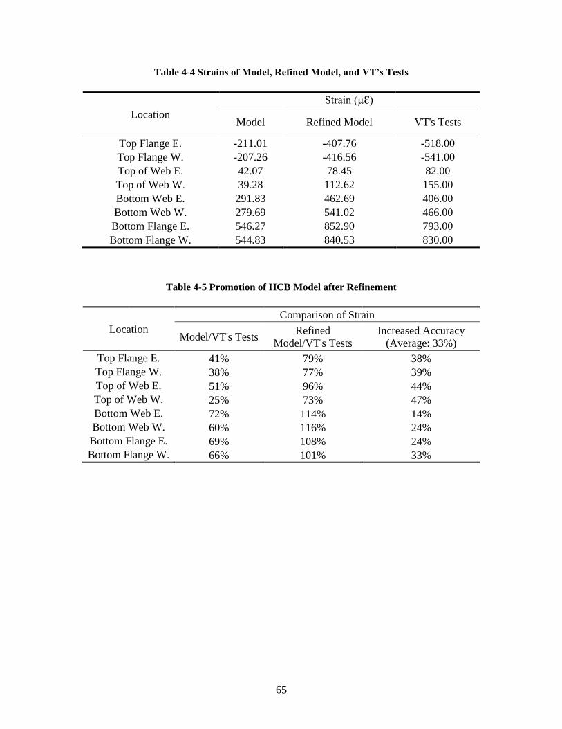
4.2.2 Refinement of HCB Model
As mentioned in section 3.4.2.10, the material properties of the bottom shell were
redefined. Figure 4-4 shows the mid-span strain at top and bottom flanges in the test
conducted on the HCB model without arch. As can be seen, the strains of HCB model
without arch were closer to the experimental results when the modulus of elasticity was
defined as 32100ksi.

64
Figure 4-4 Change of Modulus of Elasticity in Bottom Flange
As can be seen in Figure 4-5, the strains through HCB depth in the test conducted
on the full HCB model were improved by this refinement. The performance of the refined
HCB model increased 33% on average compared with the initial model (Table 4-5).
Figure 4-5 Comparison of Strains through HCB Depth
65
Table 4-4 Strains of Model, Refined Model, and VT’s Tests
Location
Strain (µƐ)
Model Refined Model VT's Tests
Top Flange E. -211.01 -407.76 -518.00
Top Flange W. -207.26 -416.56 -541.00
Top of Web E. 42.07 78.45 82.00
Top of Web W. 39.28 112.62 155.00
Bottom Web E. 291.83 462.69 406.00
Bottom Web W. 279.69 541.02 466.00
Bottom Flange E. 546.27 852.90 793.00
Bottom Flange W. 544.83 840.53 830.00
Table 4-5 Promotion of HCB Model after Refinement
Location
Comparison of Strain
Model/VT's Tests Refined
Model/VT's Tests
Increased Accuracy
(Average: 33%)
Top Flange E. 41% 79% 38%
Top Flange W. 38% 77% 39%
Top of Web E. 51% 96% 44%
Top of Web W. 25% 73% 47%
Bottom Web E. 72% 114% 14%
Bottom Web W. 60% 116% 24%
Bottom Flange E. 69% 108% 24%
Bottom Flange W. 66% 101% 33%

66
4.2.3 Results of Full HCB Model
The comparison of mid-span deflection for point load tests are shown in Table 4-6
and Error! Reference source not found.. The deflections of the model were generally l
arger than those from test results.
Table 4-6 Mid-Span Deflection for Point Load Tests
Test
Number HCB Loading (lb)
Model
(in)
Virginia Tech's
Test (in)
Ratio
Avg.(1.40)
- 1 Midspan Point Load 15000
2.23
1.56 1.43
1 1 Midspan Point Load 15000 1.54 1.45
2 1 Midspan Point Load 15000 1.65 1.35
5 2 Midspan Point Load 15000 1.59 1.40
6 2 Midspan Point Load 15000 1.53 1.46
9 3 Midspan Point Load 15000 1.70 1.31
10 3 Midspan Point Load 15000 1.57 1.42
Average for All Beams 1.59 1.40
Figure 4-6 Mid-Span Deflection for Point Load Tests

67
The comparison of mid-span deflection for quarter point load tests are shown in
Table 4-7 and Error! Reference source not found.. The deflections of the model were
generally larger than those from the test results.
Table 4-7 Mid-Span Deflection for Quarter Point Load Tests
Test
Number HCB Loading (lb)
Model
(in)
Virginia Tech's
Test (in)
Ratio
Avg.(1.40)
- 1 Quarter Point Load 12500
2.49
1.77 1.41
3 1 Quarter Point Load 12500 1.71 1.46
4 1 Quarter Point Load 12500 1.78 1.40
7 2 Quarter Point Load 12500 1.78 1.40
8 2 Quarter Point Load 12500 1.74 1.43
- 3 Quarter Point Load 12500 1.82 1.37
11 3 Quarter Point Load 12500 1.79 1.39
12 3 Quarter Point Load 12500 1.80 1.38
Average for All Beams 1.77 1.41
Figure 4-7 Mid-Span Deflection for Quarter Point Load Tests
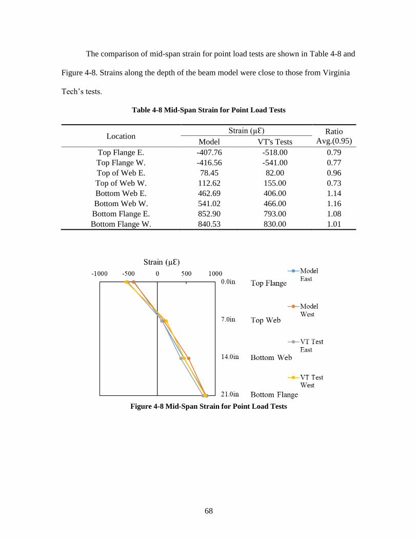
68
The comparison of mid-span strain for point load tests are shown in Table 4-8 and
Figure 4-8. Strains along the depth of the beam model were close to those from Virginia
Tech’s tests.
Table 4-8 Mid-Span Strain for Point Load Tests
Location Strain (µƐ) Ratio
Avg.(0.95) Model VT's Tests
Top Flange E. -407.76 -518.00 0.79
Top Flange W. -416.56 -541.00 0.77
Top of Web E. 78.45 82.00 0.96
Top of Web W. 112.62 155.00 0.73
Bottom Web E. 462.69 406.00 1.14
Bottom Web W. 541.02 466.00 1.16
Bottom Flange E. 852.90 793.00 1.08
Bottom Flange W. 840.53 830.00 1.01
Figure 4-8 Mid-Span Strain for Point Load Tests
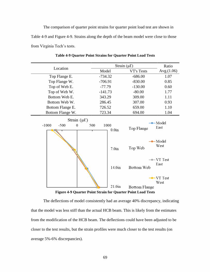
69
The comparison of quarter point strains for quarter point load test are shown in
Table 4-9 and Figure 4-9. Strains along the depth of the beam model were close to those
from Virginia Tech’s tests.
Table 4-9 Quarter Point Strains for Quarter Point Load Tests
Location Strain (µƐ) Ratio
Avg.(1.06) Model VT's Tests
Top Flange E. -734.32 -686.00 1.07
Top Flange W. -706.91 -830.00 0.85
Top of Web E. -77.79 -130.00 0.60
Top of Web W. -141.73 -80.00 1.77
Bottom Web E. 343.29 309.00 1.11
Bottom Web W. 286.45 307.00 0.93
Bottom Flange E. 726.52 659.00 1.10
Bottom Flange W. 723.34 694.00 1.04
Figure 4-9 Quarter Point Strain for Quarter Point Load Tests
The deflections of model consistently had an average 40% discrepancy, indicating
that the model was less stiff than the actual HCB beam. This is likely from the estimates
from the modification of the HCB beam. The deflections could have been adjusted to be
closer to the test results, but the strain profiles were much closer to the test results (on
average 5%-6% discrepancies).
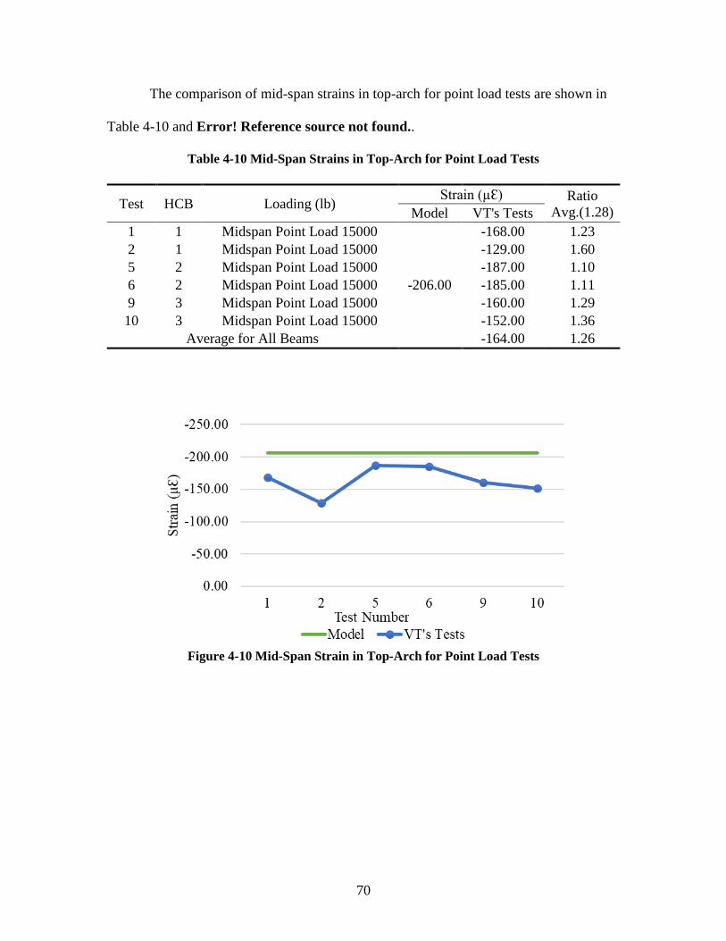
70
The comparison of mid-span strains in top-arch for point load tests are shown in
Table 4-10 and Error! Reference source not found..
Table 4-10 Mid-Span Strains in Top-Arch for Point Load Tests
Test HCB Loading (lb) Strain (µƐ) Ratio
Avg.(1.28) Model VT's Tests
1 1 Midspan Point Load 15000
-206.00
-168.00 1.23
2 1 Midspan Point Load 15000 -129.00 1.60
5 2 Midspan Point Load 15000 -187.00 1.10
6 2 Midspan Point Load 15000 -185.00 1.11
9 3 Midspan Point Load 15000 -160.00 1.29
10 3 Midspan Point Load 15000 -152.00 1.36
Average for All Beams -164.00 1.26
Figure 4-10 Mid-Span Strain in Top-Arch for Point Load Tests
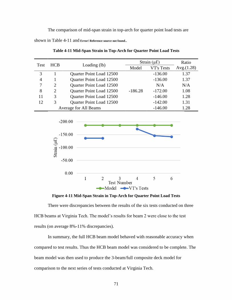
71
The comparison of mid-span strain in top-arch for quarter point load tests are
shown in Table 4-11 and Error! Reference source not found..
Table 4-11 Mid-Span Strain in Top-Arch for Quarter Point Load Tests
Test HCB Loading (lb) Strain (µƐ) Ratio
Avg.(1.28) Model VT's Tests
3 1 Quarter Point Load 12500
-186.28
-136.00 1.37
4 1 Quarter Point Load 12500 -136.00 1.37
7 2 Quarter Point Load 12500 N/A N/A
8 2 Quarter Point Load 12500 -172.00 1.08
11 3 Quarter Point Load 12500 -146.00 1.28
12 3 Quarter Point Load 12500 -142.00 1.31
Average for All Beams -146.00 1.28
Figure 4-11 Mid-Span Strain in Top-Arch for Quarter Point Load Tests
There were discrepancies between the results of the six tests conducted on three
HCB beams at Virginia Tech. The model’s results for beam 2 were close to the test
results (on average 8%-11% discrepancies).
In summary, the full HCB beam model behaved with reasonable accuracy when
compared to test results. Thus the HCB beam model was considered to be complete. The
beam model was then used to produce the 3-beam/full composite deck model for
comparison to the next series of tests conducted at Virginia Tech.

72
4.3 Three Beam/Composite Deck Model
Seventeen tests were performed in Virginia Tech’s testing based on eight load
cases. The comparison of maximum FRP strain in bottom flange is shown in Table 4-12.
The comparison of deflections is shown in Table 4-13. The comparison of maximum
strain in the concrete arch is shown in Table 4-14.
Table 4-12 Maximum FRP Strain in Bottom Flange
ST1 623.00 1.19
ST2 620.00 1.20
Model ST1&ST2 741.03 -
ST3 580.00 1.34
ST4 576.00 1.35
Model ST3&ST4 778.84 -
ST5 559.00 1.30
ST6 555.00 1.31
Model ST5&ST6 728.42 -
ST7 388.00 1.26
ST8 386.00 1.27
Model ST7&ST8 489.86 -
ST9 401.00 1.29
ST10 401.00 1.29
Model ST9&ST10 517.03 -
ST11 421.00 1.50
ST12 545.00 1.16
Model ST11&ST12 630.12 -
ST13 162.00 1.34
ST14 160.00 1.36
Model ST13&ST14 217.00 -
ST15 276.00 1.42
ST16 275.00 1.42
Model ST15&ST16 391.01 -
Test NumberStrain
(µƐ)
Ratio (Avg. 1.31)
(Model/VT)
Beam Experiencing
Max Strain in VT's
1
1
1
1
2
2
2
1
2
2
2
1
1
1
Data Source
VT's Tests
VT's Tests
VT's Tests
VT's Tests
VT's Tests
VT's Tests
VT's Tests
VT's Tests
1
2
2
2
2
2
2
1
1
1
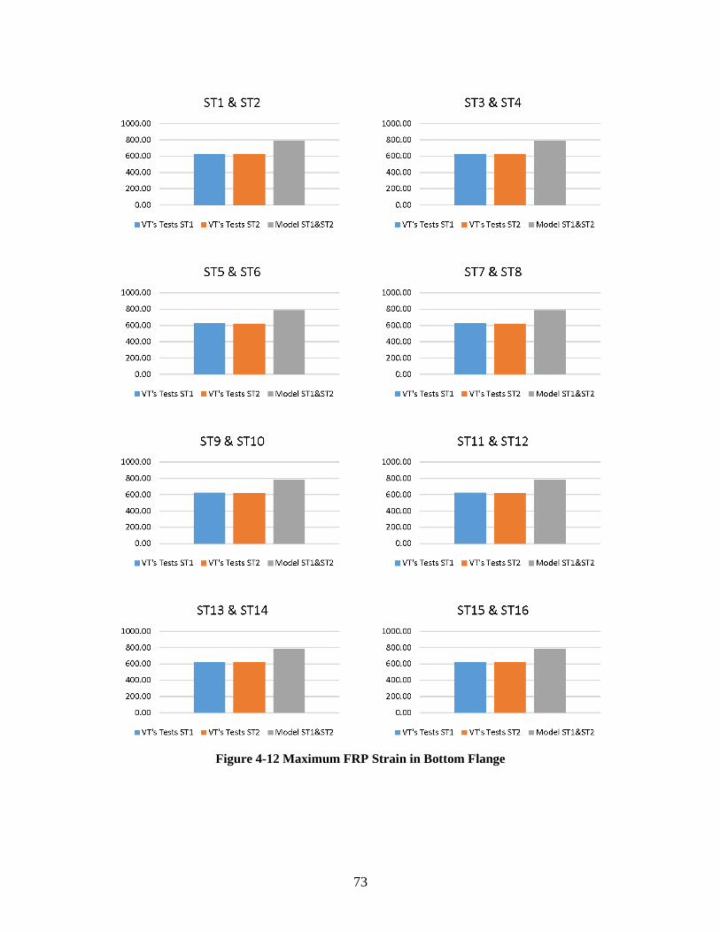
73
Figure 4-12 Maximum FRP Strain in Bottom Flange
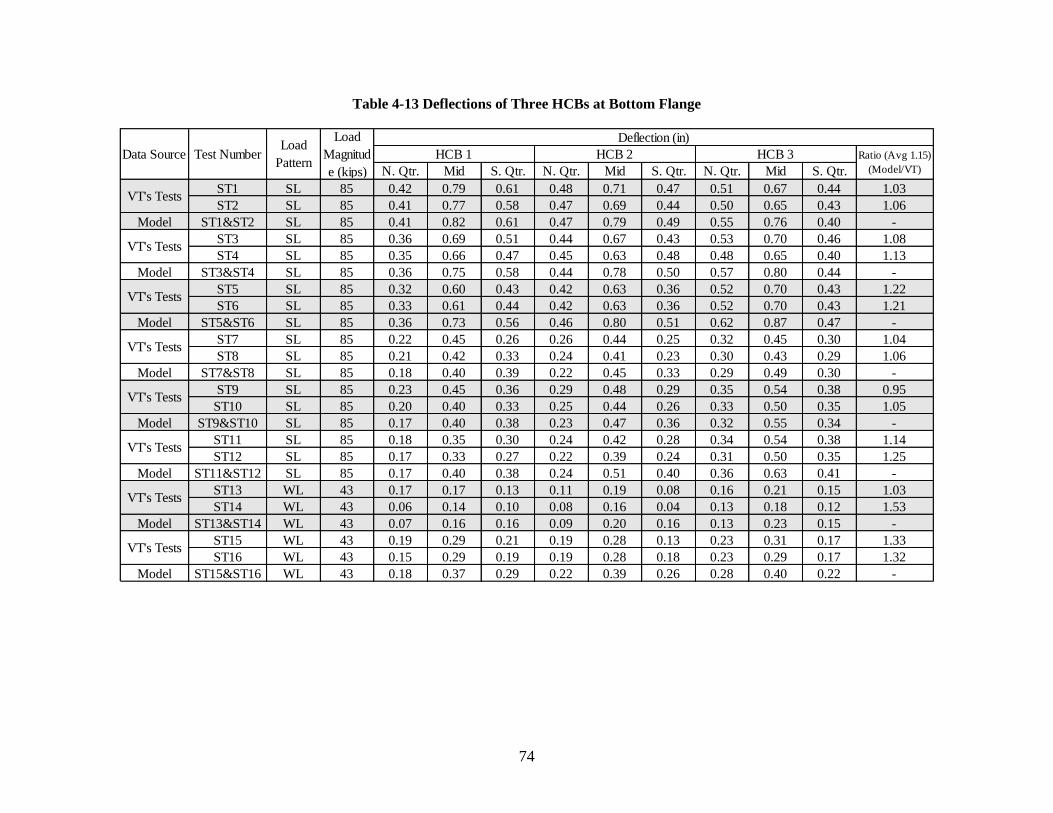
74
Table 4-13 Deflections of Three HCBs at Bottom Flange
N. Qtr. Mid S. Qtr. N. Qtr. Mid S. Qtr. N. Qtr. Mid S. Qtr.
ST1 SL 85 0.42 0.79 0.61 0.48 0.71 0.47 0.51 0.67 0.44 1.03
ST2 SL 85 0.41 0.77 0.58 0.47 0.69 0.44 0.50 0.65 0.43 1.06
Model ST1&ST2 SL 85 0.41 0.82 0.61 0.47 0.79 0.49 0.55 0.76 0.40 -
ST3 SL 85 0.36 0.69 0.51 0.44 0.67 0.43 0.53 0.70 0.46 1.08
ST4 SL 85 0.35 0.66 0.47 0.45 0.63 0.48 0.48 0.65 0.40 1.13
Model ST3&ST4 SL 85 0.36 0.75 0.58 0.44 0.78 0.50 0.57 0.80 0.44 -
ST5 SL 85 0.32 0.60 0.43 0.42 0.63 0.36 0.52 0.70 0.43 1.22
ST6 SL 85 0.33 0.61 0.44 0.42 0.63 0.36 0.52 0.70 0.43 1.21
Model ST5&ST6 SL 85 0.36 0.73 0.56 0.46 0.80 0.51 0.62 0.87 0.47 -
ST7 SL 85 0.22 0.45 0.26 0.26 0.44 0.25 0.32 0.45 0.30 1.04
ST8 SL 85 0.21 0.42 0.33 0.24 0.41 0.23 0.30 0.43 0.29 1.06
Model ST7&ST8 SL 85 0.18 0.40 0.39 0.22 0.45 0.33 0.29 0.49 0.30 -
ST9 SL 85 0.23 0.45 0.36 0.29 0.48 0.29 0.35 0.54 0.38 0.95
ST10 SL 85 0.20 0.40 0.33 0.25 0.44 0.26 0.33 0.50 0.35 1.05
Model ST9&ST10 SL 85 0.17 0.40 0.38 0.23 0.47 0.36 0.32 0.55 0.34 -
ST11 SL 85 0.18 0.35 0.30 0.24 0.42 0.28 0.34 0.54 0.38 1.14
ST12 SL 85 0.17 0.33 0.27 0.22 0.39 0.24 0.31 0.50 0.35 1.25
Model ST11&ST12 SL 85 0.17 0.40 0.38 0.24 0.51 0.40 0.36 0.63 0.41 -
ST13 WL 43 0.17 0.17 0.13 0.11 0.19 0.08 0.16 0.21 0.15 1.03
ST14 WL 43 0.06 0.14 0.10 0.08 0.16 0.04 0.13 0.18 0.12 1.53
Model ST13&ST14 WL 43 0.07 0.16 0.16 0.09 0.20 0.16 0.13 0.23 0.15 -
ST15 WL 43 0.19 0.29 0.21 0.19 0.28 0.13 0.23 0.31 0.17 1.33
ST16 WL 43 0.15 0.29 0.19 0.19 0.28 0.18 0.23 0.29 0.17 1.32
Model ST15&ST16 WL 43 0.18 0.37 0.29 0.22 0.39 0.26 0.28 0.40 0.22 -
VT's Tests
VT's Tests
VT's Tests
VT's Tests
VT's Tests
VT's Tests
VT's Tests
Test NumberLoad
Pattern
Load
Magnitud
e (kips)
Deflection (in)
HCB 1 HCB 2 HCB 3 Ratio (Avg 1.15)
(Model/VT)
VT's Tests
Data Source
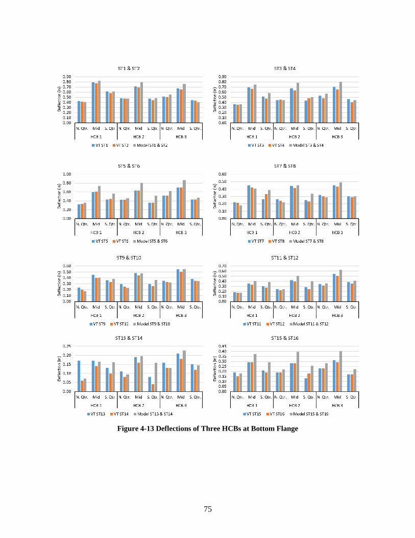
75
Figure 4-13 Deflections of Three HCBs at Bottom Flange

76
Table 4-14 Maximum Arch Strains of Three HCBs
The bold values were greater than cracking strain of 152 µƐ. These values were not consistent with the other values.
HCB 1 HCB 2 HCB 3 HCB 1 HCB 2 HCB 3 HCB 1 HCB 2 HCB 3
ST1 129.00 114.00 107.00 0.98 1578.00 N/A 403.00 - -64.00 -28.00 -14.00 -1.71
ST2 129.00 113.00 106.00 0.99 N/A N/A 402.00 - -64.00 -28.00 -13.00 -1.84
Model ST1&ST2 132.06 108.44 103.08 - 14.51 -4.43 -9.30 - -65.41 25.31 73.37 -
ST3 114.00 110.00 109.00 0.99 N/A N/A 469.00 - -44.00 -23.00 -15.00 -1.30
ST4 112.00 107.00 106.00 1.01 N/A N/A 429.00 - -46.00 -30.00 -16.00 -1.15
Model ST3&ST4 113.31 113.33 102.91 - 16.03 1.45 -6.98 - -49.32 21.15 61.31 -
ST5 103.00 108.00 110.00 0.99 N/A N/A 446.00 - 0.00 -27.00 -21.00 -1.63
ST6 101.00 106.00 108.00 1.01 N/A N/A 411.00 - -29.00 -26.00 -20.00 -0.66
Model ST5&ST6 106.89 104.94 106.83 - 15.40 0.50 -10.90 - -41.75 18.01 54.42 -
ST7 57.00 97.00 100.00 0.64 830.00 N/A 440.00 - -20.00 -14.00 -13.00 -1.28
ST8 56.00 97.00 101.00 0.64 828.00 N/A 437.00 - -20.00 -13.00 -13.00 -1.31
Model ST7&ST8 30.04 53.96 82.64 - 27.18 9.25 1.60 - -9.27 18.34 38.80 -
ST9 57.00 98.00 119.00 0.60 830.00 N/A 589.00 - -12.00 -5.00 -19.00 -1.53
ST10 56.00 97.00 119.00 0.61 N/A N/A 594.00 - -12.00 -5.00 -18.00 -1.56
Model ST9&ST10 29.83 53.49 88.69 - 26.50 12.17 3.18 - -4.80 16.59 31.91 -
ST11 45.00 72.00 110.00 0.77 902.00 N/A 537.00 - -12.00 5.00 -18.00 0.54
ST12 44.00 71.00 110.00 0.78 819.00 N/A 523.00 - -11.00 4.00 -18.00 0.79
Model ST11&ST12 30.15 53.95 97.46 - 26.29 15.26 4.89 - 1.19 15.18 23.88 -
ST13 25.00 35.00 50.00 0.55 340.00 129.00 155.00 - -6.00 6.00 -5.00 -0.18
ST14 24.00 35.00 48.00 0.57 333.00 128.00 152.00 - -6.00 5.00 -4.00 -0.30
Model ST13&ST14 10.86 18.80 33.88 - 11.36 7.19 2.76 - -2.60 11.14 14.19 -
ST15 57.00 52.00 56.00 1.00 439.00 157.00 126.00 - -16.00 -17.00 -7.00 -1.17
ST16 57.00 51.00 54.00 1.02 446.00 162.00 133.00 - -17.00 -17.00 -6.00 -1.45
Model ST15&ST16 52.26 59.13 52.94 - 7.91 2.90 -2.79 - -23.90 9.12 31.32 -
Test NumberMidspan Strains (µƐ) Ratio (avg 0.82)
(Model/VT)
Quarter Point Strains (µƐ)-
Support Strains (µƐ)Data Source
VT's Tests
VT's Tests
VT's Tests
VT's Tests
VT's Tests
VT's Tests
VT's Tests
VT's Tests
Ratio (avg -0.98)
(Model/VT)

77
Figure 4-14 Maximum Arch Strains of Three HCBs (inconsistent values not shown)
The model’s maximum FRP strains at bottom flanges were 31% on average higher than
the results from Virginia Tech’s tests. The deflections of the model at bottom flange were 15%
on average higher than the results from Virginia Tech’s tests. The maximum arch strains at mid-
span were 18% on average lower than the experimental results. The maximum arch strains at
supports shown much discrepancies, which might because of the idealized boundary condition

78
used in this model could not well simulate the boundary condition of the real structure, and the
diaphragms of the real structure were not involved in this model.
As shown above, the three-beam/composite deck model basically agreed with the testing
results from Virginia Tech’s tests. However, it may not be a good representation of the Tides
Mill Stream Bridge because of the following reasons. First, the Tides Mill Stream Bridge has
eight girders, thus the load distribution characteristics are significantly different than the three
girder system. Second, the parapets and semi-integral backwalls have significant influence on the
overall bridge stiffness, however these components were not developed in the three-
beam/composite deck model.
79
4.4 Model of Tides Mill Stream Bridge
Twelve tests were performed on the finite element model of the full bridge, based on six
load cases conducted by the University of Virginia on the completed Tides Mill Stream Bridge.
A modal analysis was also conducted on the full model and natural frequencies were compared
to those experimentally obtained from the field tests.
4.4.1 Simplifications
Two details were not modelled for simplification. First, the cross-slopes of 0.02 F/F from
the center line of the bridge to the parapets were neglected in the model construction. Second, the
small elevation difference between the northwestern and the southeastern corners of the deck
were neglected. It was felt that both details would have little or no influence on the behavior of
the model.
4.4.2 Modification on Open Deflection Joints
As mentioned in section 3.4.4.1, the open deflection joints were reflected on the initial
model of the parapets. However, these open deflection joints dramatically reduced the bending
stiffness of the parapets, thus reducing their influence on overall bridge stiffness. Hence, these
joints were removed from the final bridge model.
4.4.3 Refinement on Semi-Integral Backwalls
The performance of the bridge model increased 50% on average by refining the semi-
integral backwalls (Table 4-15).
Table 4-15 Promotion of Bridge Model after Refinement
Load Case
A B C D E F Average
72% 46% 49% 63% 41% 28% 50%

80
Figure 4-15 Comparison of Performance of Bridge Model before and after Placement of Semi-
Integral Backwalls
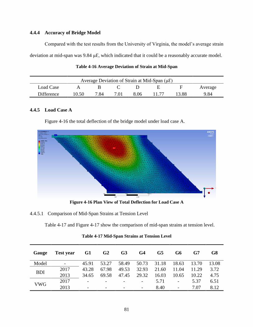
81
4.4.4 Accuracy of Bridge Model
Compared with the test results from the University of Virginia, the model’s average strain
deviation at mid-span was 9.84 µƐ, which indicated that it could be a reasonably accurate model.
Table 4-16 Average Deviation of Strain at Mid-Span
Average Deviation of Strain at Mid-Span (µƐ)
Load Case A B C D E F Average
Difference 10.50 7.84 7.01 8.06 11.77 13.88 9.84
4.4.5 Load Case A
Figure 4-16 the total deflection of the bridge model under load case A.
Figure 4-16 Plan View of Total Deflection for Load Case A
4.4.5.1 Comparison of Mid-Span Strains at Tension Level
Table 4-17 and Figure 4-17 show the comparison of mid-span strains at tension level.
Table 4-17 Mid-Span Strains at Tension Level
Gauge Test year G1 G2 G3 G4 G5 G6 G7 G8
Model - 45.91 53.27 58.49 50.73 31.18 18.63 13.70 13.08
BDI 2017 43.28 67.98 49.53 32.93 21.60 11.04 11.29 3.72
2013 34.65 69.58 47.45 29.32 16.03 10.65 10.22 4.75
VWG 2017 - - - - 5.71 - 5.37 6.51
2013 - - - - 8.40 - 7.07 8.12
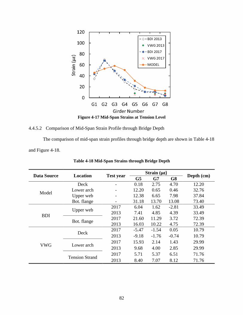
82
Figure 4-17 Mid-Span Strains at Tension Level
4.4.5.2 Comparison of Mid-Span Strain Profile through Bridge Depth
The comparison of mid-span strain profiles through bridge depth are shown in Table 4-18
and Figure 4-18.
Table 4-18 Mid-Span Strains through Bridge Depth
Data Source Location Test year Strain (µɛ)
Depth (cm) G5 G7 G8
Model
Deck - 0.18 2.75 4.70 12.20
Lower arch - 12.20 0.65 0.46 32.76
Upper web - 12.38 6.65 7.98 37.84
Bot. flange - 31.18 13.70 13.08 73.40
BDI
Upper web 2017 6.04 1.62 -2.81 33.49
2013 7.41 4.85 4.39 33.49
Bot. flange 2017 21.60 11.29 3.72 72.39
2013 16.03 10.22 4.75 72.39
VWG
Deck 2017 -5.47 -1.54 0.05 10.79
2013 -9.18 -1.76 -0.74 10.79
Lower arch 2017 15.93 2.14 1.43 29.99
2013 9.68 4.00 2.85 29.99
Tension Strand 2017 5.71 5.37 6.51 71.76
2013 8.40 7.07 8.12 71.76
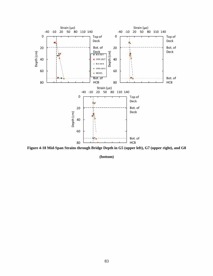
83
Figure 4-18 Mid-Span Strains through Bridge Depth in G5 (upper left), G7 (upper right), and G8
(bottom)
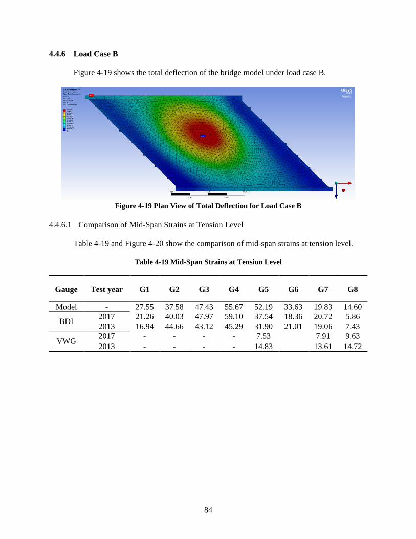
84
4.4.6 Load Case B
Figure 4-19 shows the total deflection of the bridge model under load case B.
Figure 4-19 Plan View of Total Deflection for Load Case B
4.4.6.1 Comparison of Mid-Span Strains at Tension Level
Table 4-19 and Figure 4-20 show the comparison of mid-span strains at tension level.
Table 4-19 Mid-Span Strains at Tension Level
Gauge Test year G1 G2 G3 G4 G5 G6 G7 G8
Model - 27.55 37.58 47.43 55.67 52.19 33.63 19.83 14.60
BDI 2017 21.26 40.03 47.97 59.10 37.54 18.36 20.72 5.86
2013 16.94 44.66 43.12 45.29 31.90 21.01 19.06 7.43
VWG 2017 - - - - 7.53 7.91 9.63
2013 - - - - 14.83 13.61 14.72

85
Figure 4-20 Mid-Span Strains at Tension Level
4.4.6.2 Comparison of Mid-Span Strain Profile through Bridge Depth
The comparison of mid-span strain profiles through bridge depth is shown in Table 4-20
and Figure 4-21.
Table 4-20 Mid-Span Strains through Bridge Depth
Data Source Location Test year Strain (µɛ)
Depth (cm) G5 G7 G8
Model
Deck - 0.39 2.42 4.49 12.20
Lower arch - 5.63 1.32 0.58 32.76
Upper web - 23.35 8.82 8.53 37.84
Bot. flange - 52.19 19.83 14.60 73.40
BDI
Upper web 2017 12.54 5.14 6.10 33.49
2013 19.23 7.77 6.42 33.49
Bot. flange 2017 37.54 20.72 5.86 72.39
2013 31.90 19.06 7.43 72.39
VWG
Deck 2017 -4.27 -1.91 -0.03 10.79
2013 -16.34 -2.56 -0.55 10.79
Lower arch 2017 31.78 2.98 2.45 29.99
2013 24.95 8.06 5.58 29.99
Tension Strand 2017 7.53 7.91 9.63 71.76
2013 14.83 13.61 14.72 71.76
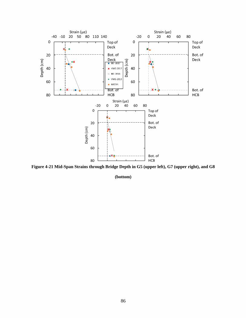
86
Figure 4-21 Mid-Span Strains through Bridge Depth in G5 (upper left), G7 (upper right), and G8
(bottom)

87
4.4.7 Load Case C
Figure 4-22 shows the total deflection of the bridge model under load case C
Figure 4-22 Plan View of Total Deflection for Load Case C
4.4.7.1 Comparison of Mid-Span Strains at Tension Level
Table 4-21 and Figure 4-23 show the comparison of mid-span strains at tension level.
Table 4-21 Mid-Span Strains at Tension Level
Data
Source Test year G1 G2 G3 G4 G5 G6 G7 G8
Model - 16.09 18.36 26.36 37.73 46.61 54.07 47.93 29.89
BDI 2017 8.24 15.61 22.09 41.15 56.34 40.68 46.94 12.43
2013 8.35 22.31 24.91 33.51 38.82 42.56 43.64 18.56
VWG 2017 - - - - 18.02 26.79 24.18
2013 - - - - 14.66 31.40 31.05
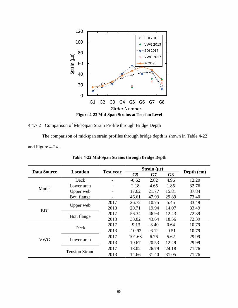
88
Figure 4-23 Mid-Span Strains at Tension Level
4.4.7.2 Comparison of Mid-Span Strain Profile through Bridge Depth
The comparison of mid-span strain profiles through bridge depth is shown in Table 4-22
and Figure 4-24.
Table 4-22 Mid-Span Strains through Bridge Depth
Data Source Location Test year Strain (µɛ)
Depth (cm) G5 G7 G8
Model
Deck - -0.62 2.82 4.96 12.20
Lower arch - 2.18 4.65 1.85 32.76
Upper web - 17.62 21.77 15.81 37.84
Bot. flange - 46.61 47.93 29.89 73.40
BDI
Upper web 2017 26.72 10.75 5.45 33.49
2013 20.71 19.94 14.07 33.49
Bot. flange 2017 56.34 46.94 12.43 72.39
2013 38.82 43.64 18.56 72.39
VWG
Deck 2017 -9.13 -3.40 0.64 10.79
2013 -10.92 -6.12 -0.51 10.79
Lower arch 2017 101.63 6.76 5.62 29.99
2013 10.67 20.53 12.49 29.99
Tension Strand 2017 18.02 26.79 24.18 71.76
2013 14.66 31.40 31.05 71.76
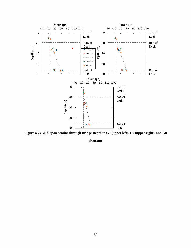
89
Figure 4-24 Mid-Span Strains through Bridge Depth in G5 (upper left), G7 (upper right), and G8
(bottom)
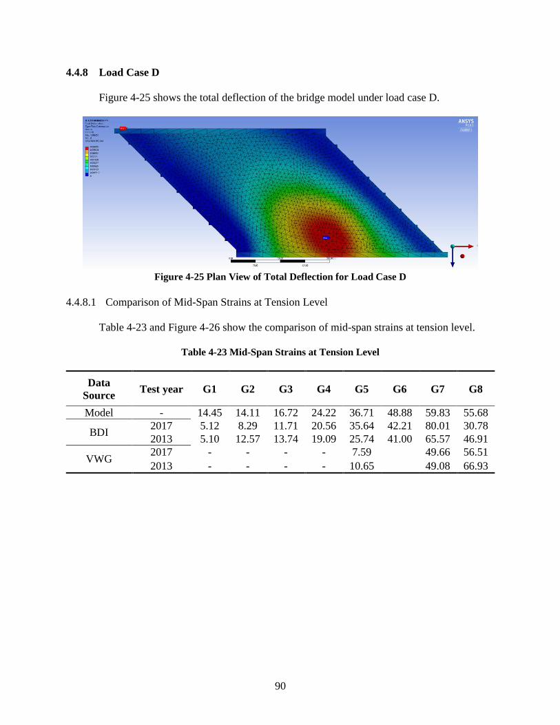
90
4.4.8 Load Case D
Figure 4-25 shows the total deflection of the bridge model under load case D.
Figure 4-25 Plan View of Total Deflection for Load Case D
4.4.8.1 Comparison of Mid-Span Strains at Tension Level
Table 4-23 and Figure 4-26 show the comparison of mid-span strains at tension level.
Table 4-23 Mid-Span Strains at Tension Level
Data
Source Test year G1 G2 G3 G4 G5 G6 G7 G8
Model - 14.45 14.11 16.72 24.22 36.71 48.88 59.83 55.68
BDI 2017 5.12 8.29 11.71 20.56 35.64 42.21 80.01 30.78
2013 5.10 12.57 13.74 19.09 25.74 41.00 65.57 46.91
VWG 2017 - - - - 7.59 49.66 56.51
2013 - - - - 10.65 49.08 66.93
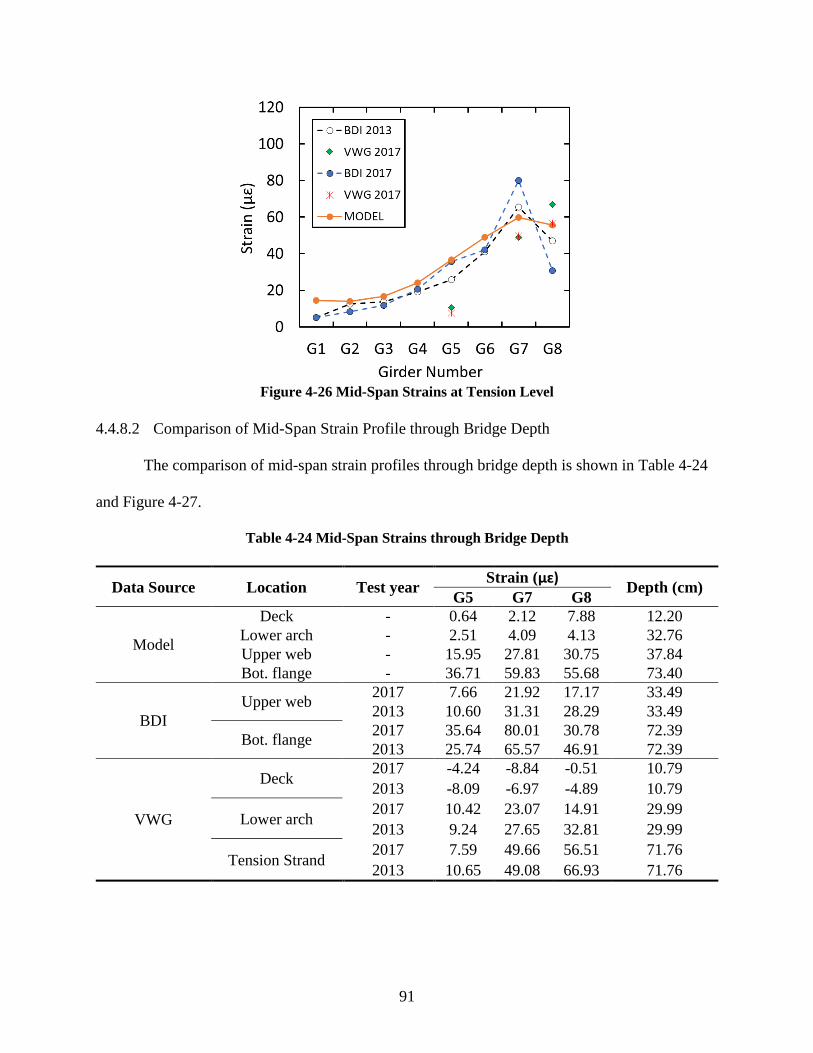
91
Figure 4-26 Mid-Span Strains at Tension Level
4.4.8.2 Comparison of Mid-Span Strain Profile through Bridge Depth
The comparison of mid-span strain profiles through bridge depth is shown in Table 4-24
and Figure 4-27.
Table 4-24 Mid-Span Strains through Bridge Depth
Data Source Location Test year Strain (µɛ)
Depth (cm) G5 G7 G8
Model
Deck - 0.64 2.12 7.88 12.20
Lower arch - 2.51 4.09 4.13 32.76
Upper web - 15.95 27.81 30.75 37.84
Bot. flange - 36.71 59.83 55.68 73.40
BDI
Upper web 2017 7.66 21.92 17.17 33.49
2013 10.60 31.31 28.29 33.49
Bot. flange 2017 35.64 80.01 30.78 72.39
2013 25.74 65.57 46.91 72.39
VWG
Deck 2017 -4.24 -8.84 -0.51 10.79
2013 -8.09 -6.97 -4.89 10.79
Lower arch 2017 10.42 23.07 14.91 29.99
2013 9.24 27.65 32.81 29.99
Tension Strand 2017 7.59 49.66 56.51 71.76
2013 10.65 49.08 66.93 71.76
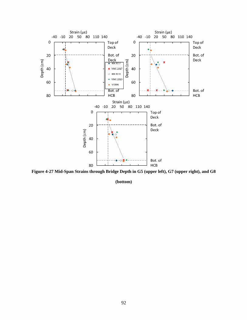
92
Figure 4-27 Mid-Span Strains through Bridge Depth in G5 (upper left), G7 (upper right), and G8
(bottom)
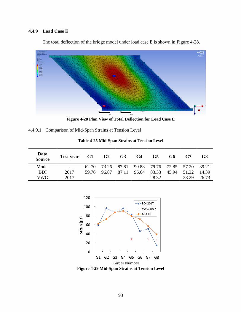
93
4.4.9 Load Case E
The total deflection of the bridge model under load case E is shown in Figure 4-28.
Figure 4-28 Plan View of Total Deflection for Load Case E
4.4.9.1 Comparison of Mid-Span Strains at Tension Level
Table 4-25 Mid-Span Strains at Tension Level
Data
Source Test year G1 G2 G3 G4 G5 G6 G7 G8
Model - 62.70 73.26 87.81 90.88 79.76 72.85 57.20 39.21
BDI 2017 59.76 96.87 87.11 96.64 83.33 45.94 51.32 14.39
VWG 2017 - - - - 28.32 28.29 26.73
Figure 4-29 Mid-Span Strains at Tension Level

94
4.4.9.2 Comparison of Mid-Span Strain Profile through Bridge Depth
Table 4-26 Mid-Span Strains through Bridge Depth
Data Source Location Test year Strain (µƐ)
Depth (cm) G5 G7 G8
Model
Deck - -0.34 5.63 9.43 12.20
Lower arch - 5.27 4.88 1.96 32.76
Upper web - 30.97 26.15 21.87 37.84
Bot. flange - 79.76 57.20 39.21 73.40
BDI Upper web
2017 37.02 11.55 12.35 33.49
Bot. flange 83.33 51.32 14.39 72.39
VWG
Deck
2017
-19.43 -4.09 -0.40 10.79
Lower arch 127.97 6.99 5.83 29.99
Tension Strand 28.32 28.29 26.73 71.76
Figure 4-30 Mid-Span Strains through Bridge Depth in G5 (upper left), G7 (upper right), and G8
(bottom)
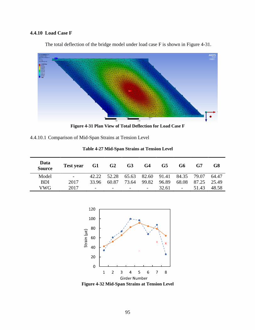
95
4.4.10 Load Case F
The total deflection of the bridge model under load case F is shown in Figure 4-31.
Figure 4-31 Plan View of Total Deflection for Load Case F
4.4.10.1 Comparison of Mid-Span Strains at Tension Level
Table 4-27 Mid-Span Strains at Tension Level
Data
Source Test year G1 G2 G3 G4 G5 G6 G7 G8
Model - 42.22 52.28 65.63 82.60 91.41 84.35 79.07 64.47
BDI 2017 33.96 60.87 73.64 99.82 96.89 68.08 87.25 25.49
VWG 2017 - - - - 32.61 - 51.43 48.58
Figure 4-32 Mid-Span Strains at Tension Level
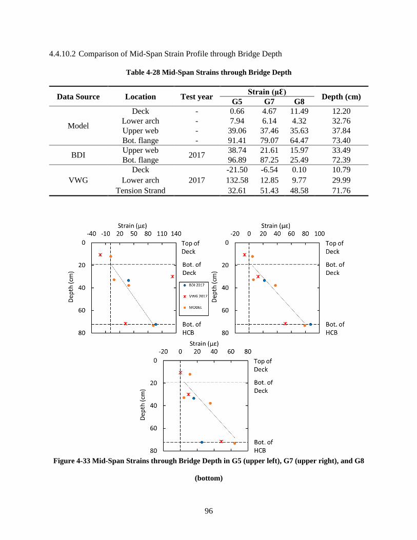
96
4.4.10.2 Comparison of Mid-Span Strain Profile through Bridge Depth
Table 4-28 Mid-Span Strains through Bridge Depth
Data Source Location Test year Strain (µƐ)
Depth (cm) G5 G7 G8
Model
Deck - 0.66 4.67 11.49 12.20
Lower arch - 7.94 6.14 4.32 32.76
Upper web - 39.06 37.46 35.63 37.84
Bot. flange - 91.41 79.07 64.47 73.40
BDI Upper web
2017 38.74 21.61 15.97 33.49
Bot. flange 96.89 87.25 25.49 72.39
VWG
Deck
2017
-21.50 -6.54 0.10 10.79
Lower arch 132.58 12.85 9.77 29.99
Tension Strand 32.61 51.43 48.58 71.76
Figure 4-33 Mid-Span Strains through Bridge Depth in G5 (upper left), G7 (upper right), and G8
(bottom)
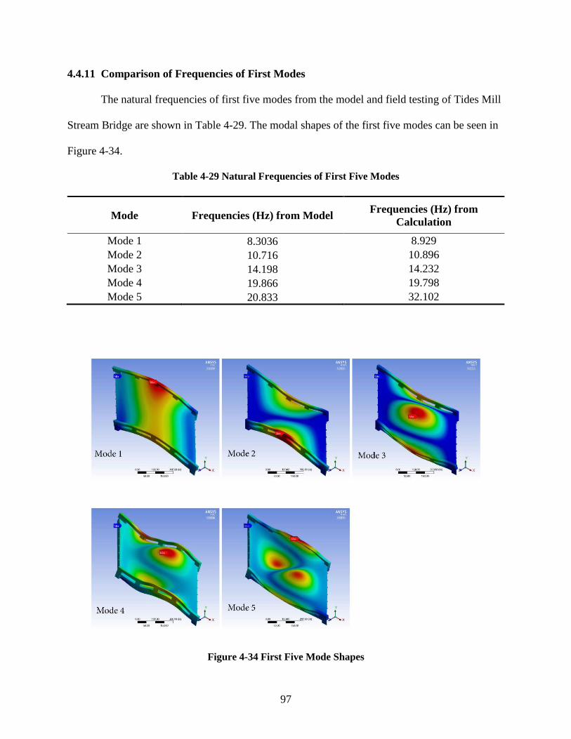
97
4.4.11 Comparison of Frequencies of First Modes
The natural frequencies of first five modes from the model and field testing of Tides Mill
Stream Bridge are shown in Table 4-29. The modal shapes of the first five modes can be seen in
Figure 4-34.
Table 4-29 Natural Frequencies of First Five Modes
Mode Frequencies (Hz) from Model Frequencies (Hz) from
Calculation
Mode 1 8.3036 8.929
Mode 2 10.716 10.896
Mode 3 14.198 14.232
Mode 4 19.866 19.798
Mode 5 20.833 32.102
Figure 4-34 First Five Mode Shapes

98
5 Conclusions and Recommendations
5.1 Conclusions
The full HCB beam model behaved with reasonable accuracy when compared to Virginia
Tech’s test results. The strain profiles were close to the test results (on average 5%-6%
discrepancies). However, the deflections of the model consistently averaged 40% higher,
indicating that the model was less stiff than the actual HCB beam. Because strain data, and not
deflection data, were available from the Tides Mill bridge field testing, it was determined to
proceed with the HCB model without further refinement for the development of the full Tides
Mill bridge model.
The model of Tides Mill Stream Bridge is a reasonably accurate model compared with
the test results from the University of Virginia. The model’s average strain deviation at mid-span
was 9.84 µƐ. A means of determining accuracy of finite element models of complex systems is
to compare natural frequencies of the model, obtained from a modal analysis, to those
frequencies determine experimentally. The natural frequencies of a physical system are a
function of the square root of the system’s global stiffness to its mass. Mass is fairly simple to
obtain. All one needs to know are system geometries and constituent material densities. The
difficult is in determining a system’s global stiffness. The natural frequencies of the Tides Mill
finite element model compare very favorably to those obtained from experimentation. Thus
indicating, at least to some degree quantitatively, the closeness of the global model stiffness to
that of the actual bridge structure. The close natural frequencies of the first four modes indicated
that the bridge model could be a rational simulation of the Tides Mill Stream Bridge.
99
5.2 Recommendations
Improvements to the HCB beam model may result from better understanding of the
complex surface connection conditions between the composite material shell and the concrete
arch and the bottom flange of the shell and the steel strands. This would require significant mesh
refinement and the need to conduct non-linear analyses. Both would represent significant
requirements of computational resources. A second recommendation is to focus a study on
simplifying the HCB model by developing a detailed “transformed section” methodology. The
simplified HCB model could then be used to create another model of the Tides Mill Stream
Bridge. From this transformed section model, it is recommended to conduct a series of load tests
to determine its accuracy to the field test data. This could lead to a simplified design approach
for the enhanced use of this novel beam. Additionally, the simplified model could be used by
bridge management personnel to better assess in-service condition states for maintenance
decisions. It is recommended to conduct a thermal load analysis of the Tides Mill model, to
include backfill soil characteristics, in order to better understand soil/structure interaction of the
semi-integral bridge design. Finally, a series of moving load tests should be conducted and
results compared to the dynamic load tests conducted by the University of Virginia to better
understand load distribution and dynamic load factor for this novel bridge system.
100
References
Ahsan, S. (2012). Evaluation of Hybrid-Composite Beam for Use in Tide Mill Bridge. Master of
Science Thesis, Blacksburg, Virginia.
Biggs, R. M., Barton, F. W., Gomez, J. P., Massarelli, P. J., & McKeel, W. T. (2000). FINITE
ELEMENT MODELING AND ANALYSIS OF REINFORCED-CONCRETE BRIDGE
DECKS. Charlottesville: Virginia Transportation Research Council.
Cai, C. S., Oghumu, S. O., & Meggers, D. A. (2009). Finite-Element Modeling and Development
of Equivalent Properties for FRP Bridge Panels. Journal of Bridge Engineering, 14(2),
10.
Civitillo, J. M. (2014). IN-SERVICE PERFORMANCE AND BEHAVIOR CHARACTERIZATION
OF THE HYBRIDCOMPOSITE BRIDGE SYSTEM. Master of Science Thesis,
Charlottesville, Virginia.
Harris, D. K., Civitillo, J. M., & Gheitasi, A. (2016). Performance and Behavior of Hybrid
Composite Beam Bridgein Virginia: Live Load Testing. Journal of Bridge Engineering,
21(6), 16022-1 - 16036-1. doi:10.1061/(ASCE)BE.1943-5592.0000820
Hillman, J. (2003). Investigation of a Hybrid-Composite Beam System. Washington:
Transportation Research Board.
Hillman, J. (2008). Product Application of a Hybrid-Composite Beam System. Washington:
Transportation Research Board.
101
Jr, J. M. (2014). IN-SERVICE PERFORMANCE AND BEHAVIOR CHARACTERIZATION OF
THE HYBRIDCOMPOSITE BRIDGE SYSTEM. Master of Science Thesis,
Charlottesville, Virginia.
Machado, M. A., Sotelino, E. D., & Liu, J. (2008). Modeling Technique for Honeycomb FRP
Deck Bridges via Finite Elements. JOURNAL OF STRUCTURAL ENGINEERING,
134(4), 9.
Myers, M. A. (2015). Finite-Element Modeling of Hybrid Composite Beam Bridges in Missouri.
Journal of Bridge Engineering, 20(1), 11. doi:10.1061/(ASCE)BE.1943-5592.0000635
Nosdall, S. V. (2013). Experiments on a Hybrid Composite Beam for Bridge Applications .
Master of Science Thesis, Blacksburg, VA .
Slade, R., & Eriksson, R. (2012). Rte 205 over Tide Mill Stream. Engineering Report.
Snape, T., & Lindyberg, R. (2009). Test Results: HC Beam for the Knickerbocker Bridge .
AEWC Report 10-15 Project 671.
Tuwair, H., Volz, J., Mohamed A. ElGawady, M., Chandrashekhara, K., & Birman, a. V. (2016).
Modeling and Analysis of GFRP Bridge Deck Panels Filled with Polyurethane Foam.
Journal of Bridge Engineering, 21(5). doi:10.1061/(ASCE)BE.1943-5592.0000849
Related Documents


