15-Power Curve ECEGR 452 Renewable Energy Systems

Welcome message from author
This document is posted to help you gain knowledge. Please leave a comment to let me know what you think about it! Share it to your friends and learn new things together.
Transcript

15-Power Curve
ECEGR 452
Renewable Energy Systems
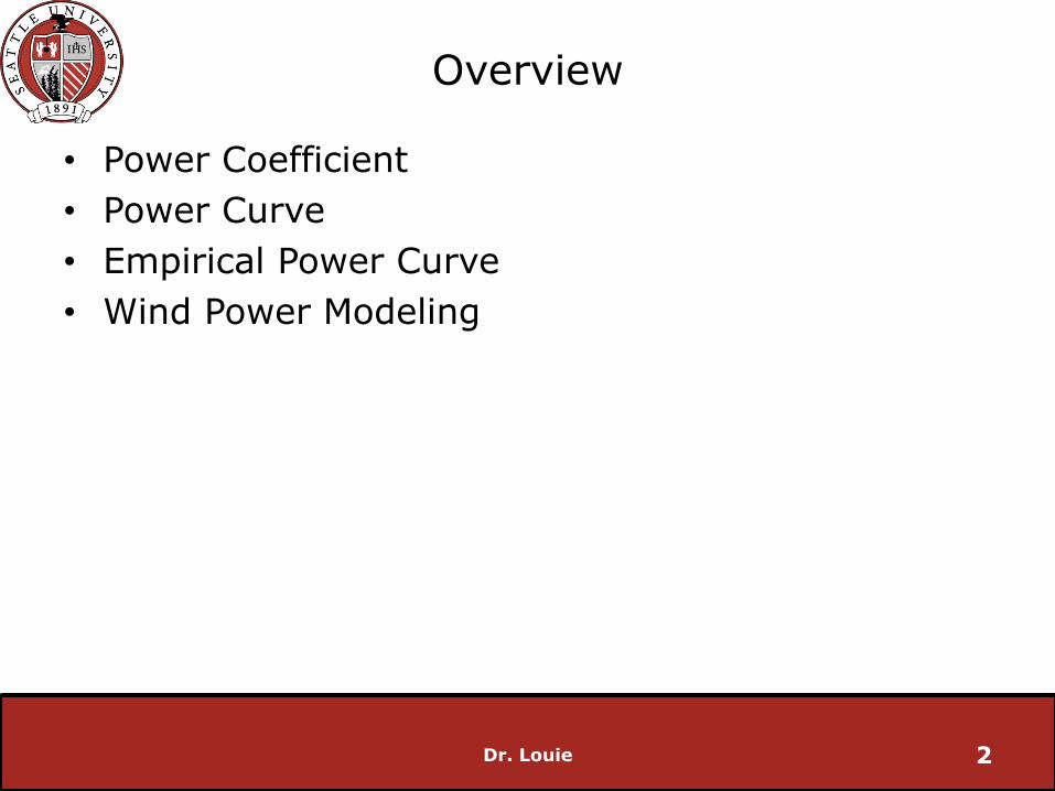
Overview
• Power Coefficient
• Power Curve
• Empirical Power Curve
• Wind Power Modeling
2 Dr. Louie

Power Coefficient
• Recall the power in a mass of moving air is:
• Mechanical power available is:
• Cp: is the unitless power coefficient (more on this in the next lecture)
Dr. Louie 3
31
2p
P C A v
31
2P A v

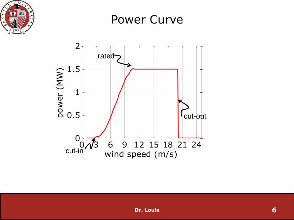
Power Curve
• Relationship between power output of a wind turbine and the wind speed is known as the Power Curve
• Power Curve depends on wind turbine type, model, manufacturer
Dr. Louie 4

Power Curve
• Power curve is dictated by:
Cut in wind speed: minimum wind speed for power generation
Cut out wind speed: maximum wind speed for which the wind turbine produces power
Rated wind speed: wind speed at which the wind turbine produces rated (nameplate) power
• Also density of the air
We will assume it is constant
Dr. Louie 5
0 3 6 9 12 15 18 21 240
0.5
1
1.5
2
pow
er
(MW
)
wind speed (m/s)
Power Curve
Dr. Louie 6
cut-in
cut-out
rated

Power Curve
Dr. Louie 7
GE 1.5MW Product Brochure

Power Curve
• For a given wind speed, the power output of a wind turbine can be computed directly from the power curve
• Power curve is non-linear
• Subdivide it into four regions
• Compute power output based upon region
Dr. Louie 8
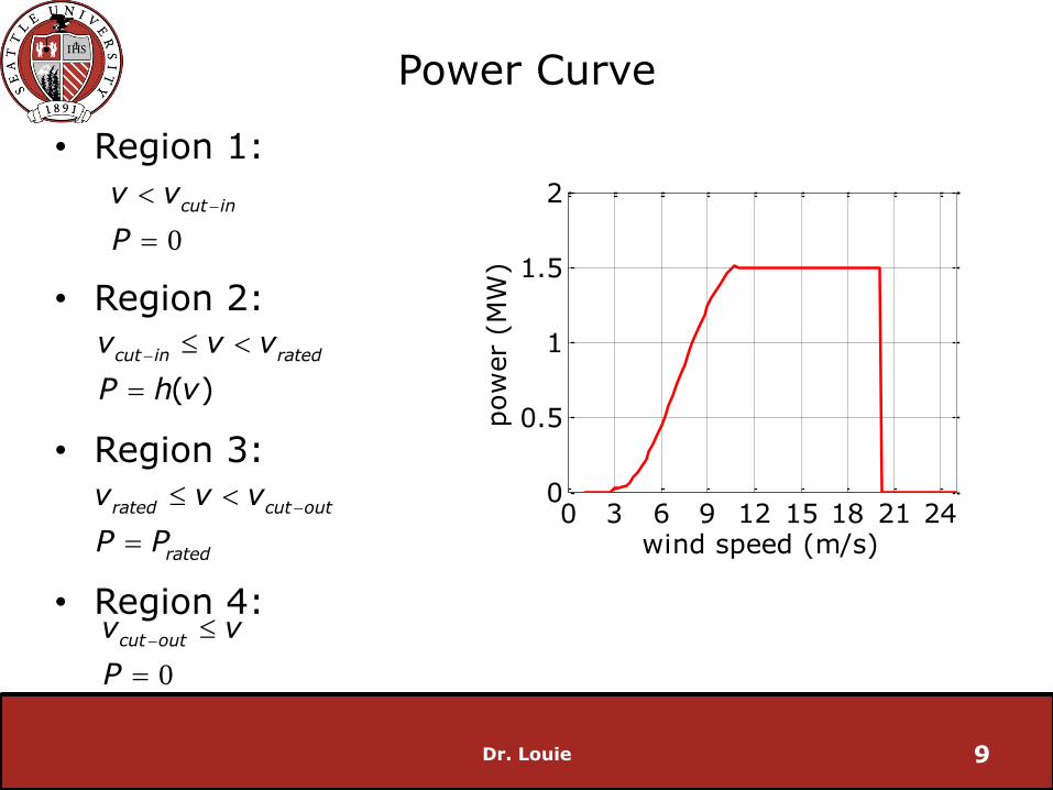
Power Curve
• Region 1:
• Region 2:
• Region 3:
• Region 4:
Dr. Louie 9
0
cut inv v
P
( )
cut in ratedv v v
P h v
rated cut out
rated
v v v
P P
0
cut outv v
P
0 3 6 9 12 15 18 21 240
0.5
1
1.5
2
pow
er
(MW
)
wind speed (m/s)

Below Cut-In
• At low wind speeds no electrical power is produced
• Cp is zero
• Power in the wind is not enough to either overcome the friction of the drivetrain, or to result in positive net power production
Dr. Louie 10
0 3 6 9 12 15 18 21 240
0.5
1
1.5
2
pow
er
(MW
)
wind speed (m/s)
31
2p
P C A v
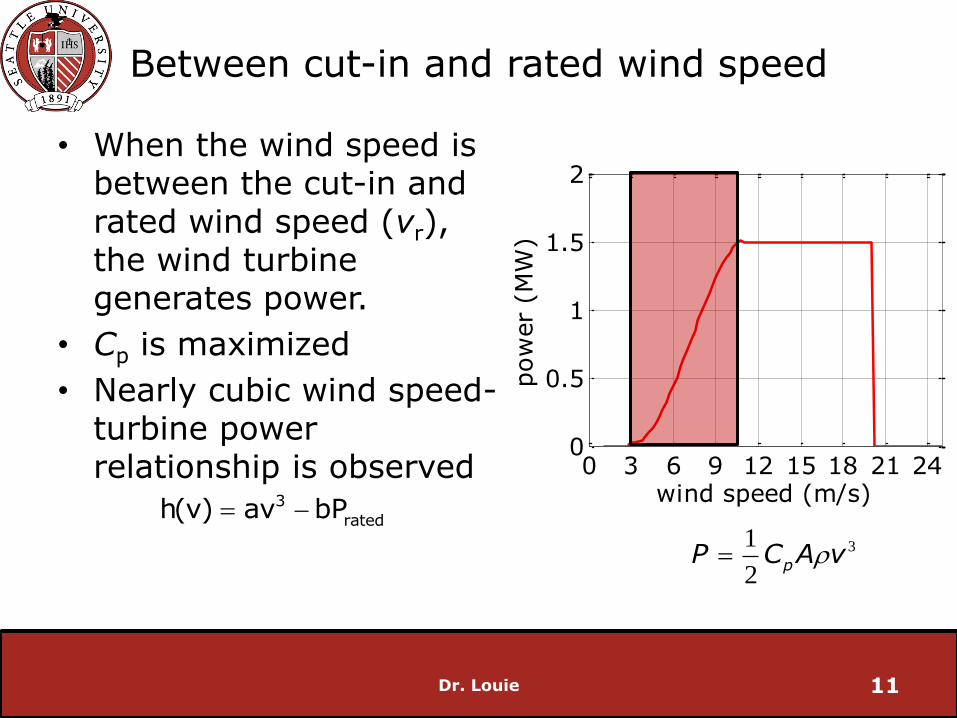
Between cut-in and rated wind speed
• When the wind speed is between the cut-in and rated wind speed (vr), the wind turbine generates power.
• Cp is maximized
• Nearly cubic wind speed-turbine power relationship is observed
Dr. Louie 11
0 3 6 9 12 15 18 21 240
0.5
1
1.5
2
pow
er
(MW
)
wind speed (m/s)
31
2p
P C A v
3
ratedh(v) av bP
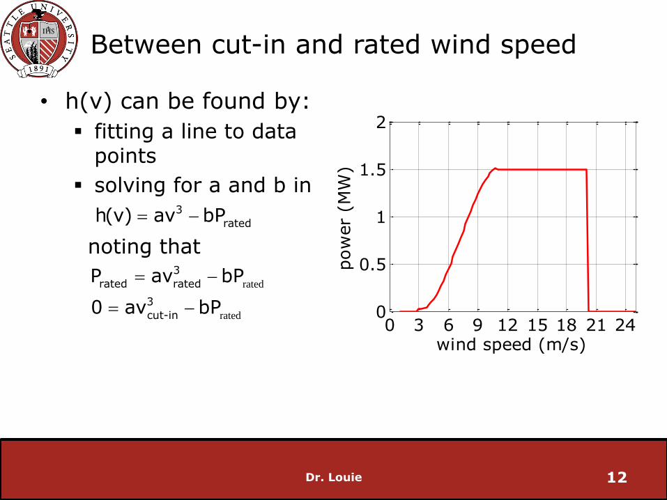
Between cut-in and rated wind speed
• h(v) can be found by:
fitting a line to data points
solving for a and b in
noting that
Dr. Louie 12
0 3 6 9 12 15 18 21 240
0.5
1
1.5
2
pow
er
(MW
)wind speed (m/s)
3
ratedh(v) av bP
rated
rated
3
rated rated
3
cut-in
P av bP
0 av bP

Between rated and cut-out wind speed
• At wind speeds above rated and below cut-out (vco), the wind turbine is controlled to maintain constant power production.
• Constant power is maintained by reducing Cp through active pitch control or passive stall design
Dr. Louie 13
0 3 6 9 12 15 18 21 240
0.5
1
1.5
2
pow
er
(MW
)
wind speed (m/s)
31
2p
P C A v
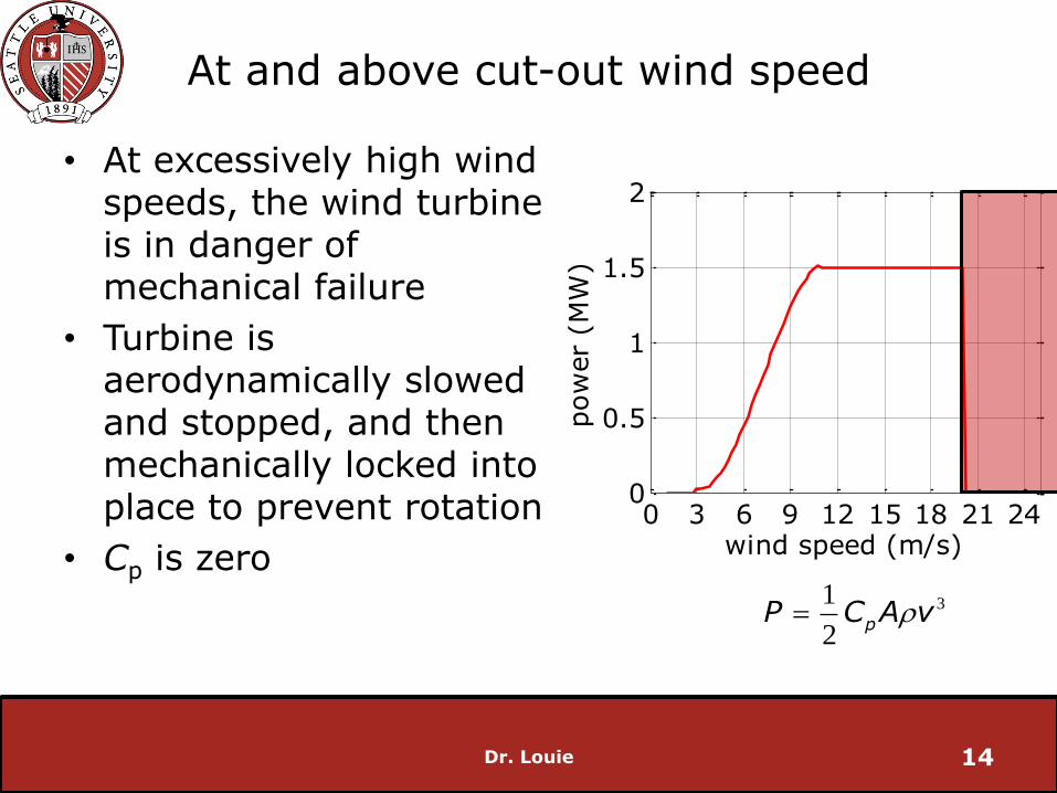
At and above cut-out wind speed
• At excessively high wind speeds, the wind turbine is in danger of mechanical failure
• Turbine is aerodynamically slowed and stopped, and then mechanically locked into place to prevent rotation
• Cp is zero
Dr. Louie 14
0 3 6 9 12 15 18 21 240
0.5
1
1.5
2
pow
er
(MW
)
wind speed (m/s)
31
2p
P C A v

Wind Power Modeling
Dr. Louie 15
0 4 8 12 18 240
5
10
15
20
25
win
d s
peed (
m/s
)
time (hr)
Region
4
3
2
1
GE 1.5XLE

Wind Power Modeling
Dr. Louie 16
0 4 8 12 18 240
0.5
1
1.5
2
pow
er
(MW
)
time (hr)
0 4 8 12 18 240
5
10
15
20
25
win
d s
peed (
m/s
)
time (hr)

Match the Power Output with the Wind Speed
Dr. Louie 17
0 4 8 12 18 240
5
10
15
20
25
win
d s
peed (
m/s
)
time (hr)0 4 8 12 18 24
0
0.5
1
1.5
2
pow
er
(MW
)
time (hr)
0 4 8 12 18 240
0.5
1
1.5
2
pow
er
(MW
)
time (hr)0 4 8 12 18 24
0
0.5
1
1.5
2
pow
er
(MW
)
time (hr)

Match the Power Output with the Wind Speed
Dr. Louie 18
0 4 8 12 18 240
5
10
15
20
25
win
d s
peed (
m/s
)
time (hr)0 4 8 12 18 24
0
0.5
1
1.5
2
pow
er
(MW
)
time (hr)
0 4 8 12 18 240
0.5
1
1.5
2
pow
er
(MW
)
time (hr)0 4 8 12 18 24
0
0.5
1
1.5
2
pow
er
(MW
)
time (hr)

Match the Power Output with the Wind Speed
Dr. Louie 19
0 4 8 12 18 240
5
10
15
20
25
win
d s
peed (
m/s
)
time (hr)
0 4 8 12 18 240
0.5
1
1.5
2
pow
er
(MW
)
time (hr)
0 4 8 12 18 240
0.5
1
1.5
2
pow
er
(MW
)
time (hr)
0 4 8 12 18 240
0.5
1
1.5
2
pow
er
(MW
)
time (hr)

Match the Power Output with the Wind Speed
Dr. Louie 20
0 4 8 12 18 240
5
10
15
20
25
win
d s
peed (
m/s
)
time (hr)
0 4 8 12 18 240
0.5
1
1.5
2
pow
er
(MW
)
time (hr)
0 4 8 12 18 240
0.5
1
1.5
2
pow
er
(MW
)
time (hr)
0 4 8 12 18 240
0.5
1
1.5
2
pow
er
(MW
)
time (hr)
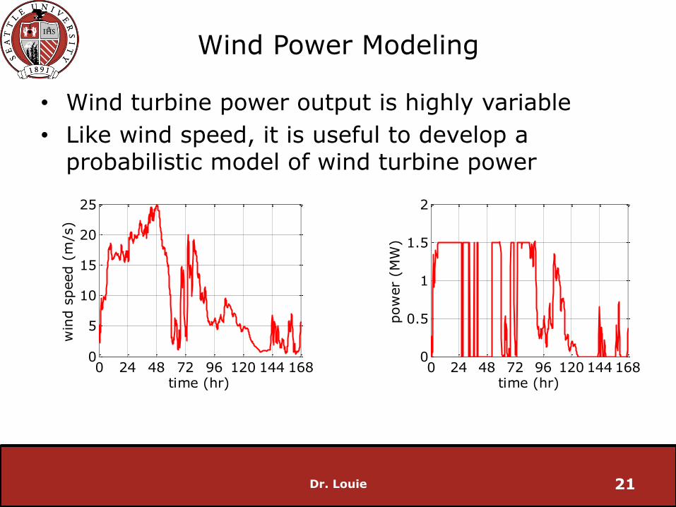
Wind Power Modeling
• Wind turbine power output is highly variable
• Like wind speed, it is useful to develop a probabilistic model of wind turbine power
Dr. Louie 21
0 24 48 72 96 120 144 1680
0.5
1
1.5
2
pow
er
(MW
)time (hr)
0 24 48 72 96 120 144 1680
5
10
15
20
25
win
d s
peed (
m/s
)
time (hr)

Empirical Power Curve
Dr. Louie 22
What causes departures in Power production from the power curve?

Wind Power Modeling
• Assume the following histogram of wind speed distribution is given for a potential wind plant
• How much energy will be produced each year?
VERY important for financing the project
Dr. Louie 23
0 20 400
2000
4000
6000
8000
10-M
inute
Occurr
ences/Y
r
wind speed (m/s)
Wind Power Modeling
• We want the PDF of the power output
Let P = g(v)
g is a function representing the power curve
Assume that we will first consider the GE 1.5XLE model
• PDF of power output can be found by computing f(P) = f(g(v))
Dr. Louie 24

Wind Power Modeling
Dr. Louie 25
0 0.5 1 1.50
0.5
1
1.5
2
2.5x 10
4
10-M
inute
Occurr
ences/Yr
power output (MW)
0 20 400
2000
4000
6000
8000
10000
10-M
inute
Occurr
ences/Y
r
wind speed (m/s)
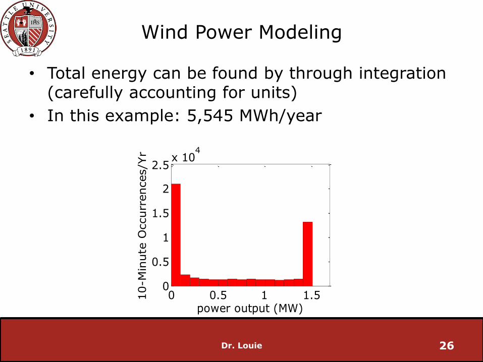
Wind Power Modeling
• Total energy can be found by through integration (carefully accounting for units)
• In this example: 5,545 MWh/year
Dr. Louie 26
0 0.5 1 1.50
0.5
1
1.5
2
2.5x 10
410-M
inute
Occurr
ences/Yr
power output (MW)
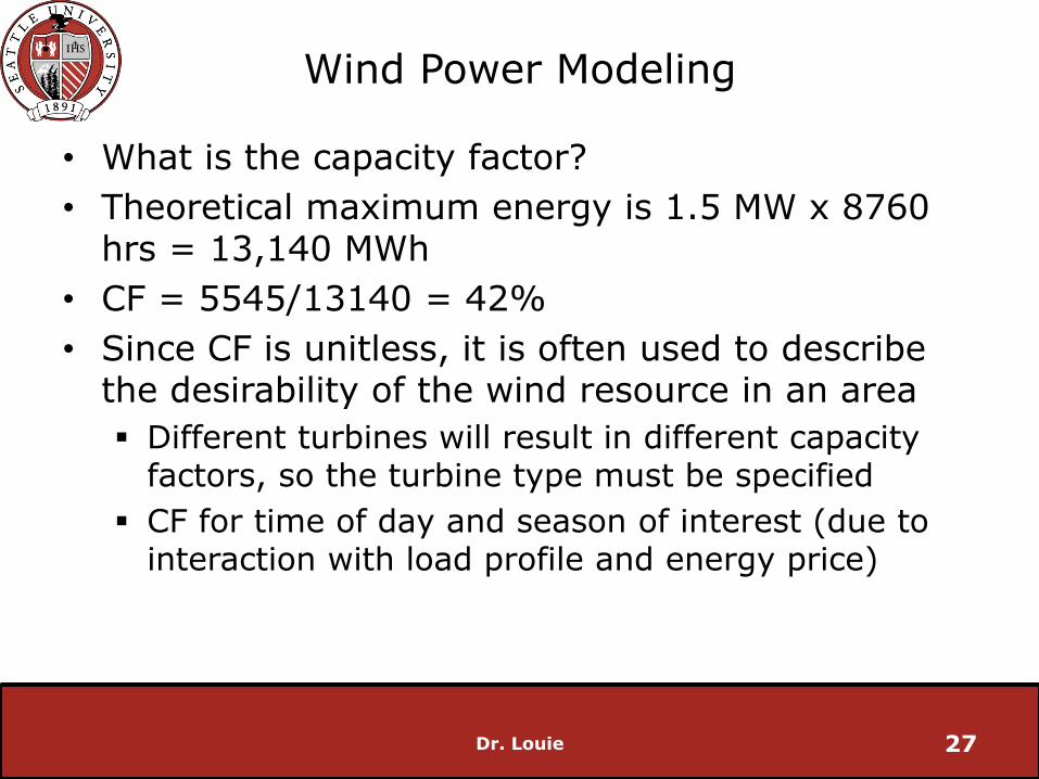
Wind Power Modeling
• What is the capacity factor?
• Theoretical maximum energy is 1.5 MW x 8760 hrs = 13,140 MWh
• CF = 5545/13140 = 42%
• Since CF is unitless, it is often used to describe the desirability of the wind resource in an area
Different turbines will result in different capacity factors, so the turbine type must be specified
CF for time of day and season of interest (due to interaction with load profile and energy price)
Dr. Louie 27
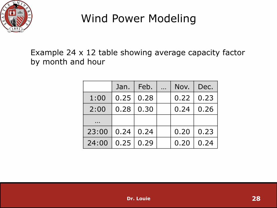
Wind Power Modeling
Jan. Feb. … Nov. Dec.
1:00 0.25 0.28 0.22 0.23
2:00 0.28 0.30 0.24 0.26
…
23:00 0.24 0.24 0.20 0.23
24:00 0.25 0.29 0.20 0.24
Dr. Louie 28
Example 24 x 12 table showing average capacity factor by month and hour
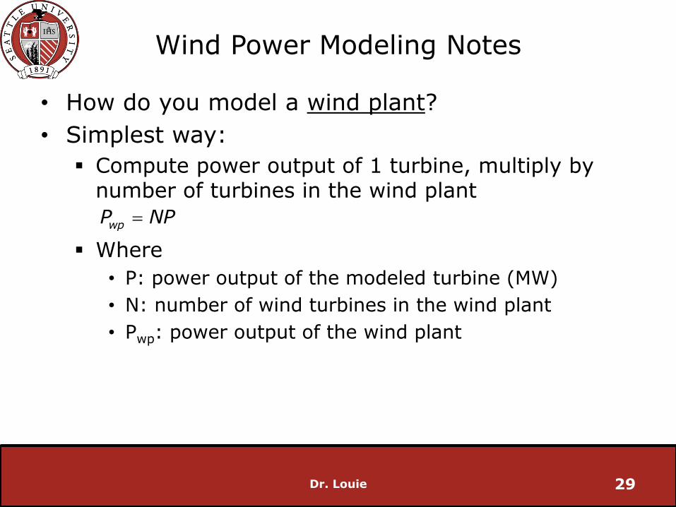
Wind Power Modeling Notes
• How do you model a wind plant?
• Simplest way:
Compute power output of 1 turbine, multiply by number of turbines in the wind plant
Where
• P: power output of the modeled turbine (MW)
• N: number of wind turbines in the wind plant
• Pwp: power output of the wind plant
Dr. Louie 29
wpP NP

Dr. Louie 30
wind turbines
1.3 miles
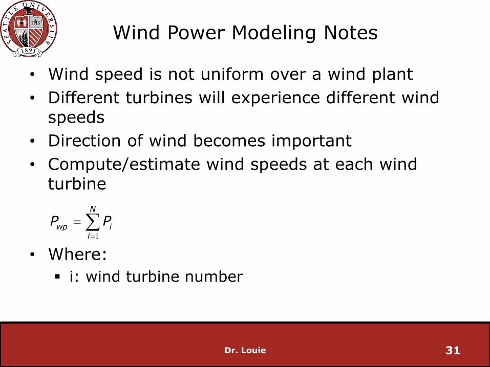
Wind Power Modeling Notes
• Wind speed is not uniform over a wind plant
• Different turbines will experience different wind speeds
• Direction of wind becomes important
• Compute/estimate wind speeds at each wind turbine
• Where:
i: wind turbine number
Dr. Louie 31
1
N
wp ii
P P
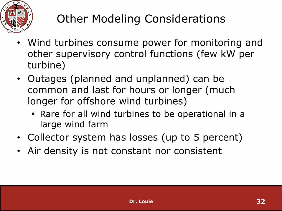
Other Modeling Considerations
• Wind turbines consume power for monitoring and other supervisory control functions (few kW per turbine)
• Outages (planned and unplanned) can be common and last for hours or longer (much longer for offshore wind turbines)
Rare for all wind turbines to be operational in a large wind farm
• Collector system has losses (up to 5 percent)
• Air density is not constant nor consistent
Dr. Louie 32
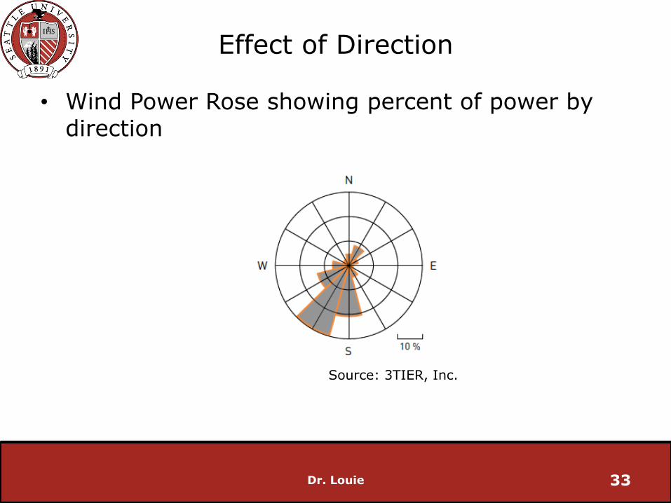
Effect of Direction
• Wind Power Rose showing percent of power by direction
Dr. Louie 33
Source: 3TIER, Inc.
Reading
R. Thresher, M. Robinson and P. Veers “To Capture the Wind”, IEEE Power & Energy Magazine, Vol. 5, No. 6, Dec 2007
Dr. Louie 34
Related Documents