1497650X

8/6/2019 1497650X

http://slidepdf.com/reader/full/1497650x 1/12

Use of highly efficient Draper Á /Lin small composite designs in

the formal optimisation of both operational and chemical

crucial variables affecting a FIA-chemiluminescence detection

system

Laura Gamiz-Gracia *, Luis Cuadros-Rodrıguez, Eva Almansa-Lopez,Jorge J. Soto-Chinchilla, Ana M. Garcıa-Campana

Department of Analytical Chemistry, School of Qualimetrics, Uni versity of Granada, E-18071 Granada, Spain

Received 23 July 2002; received in revised form 25 November 2002; accepted 20 December 2002

Abstract

A new formal strategy in the multidimensional optimisation of the experimental variables affecting the

chemiluminescence (CL) detection in flow injection analysis (FIA) is proposed here. The strategy implies severalsteps, being the most significant: selection of the variables to be studied and their experimental domain; use of a

screening design to detect significant variables and interactions into the experimental region; study of the main effect of

variables and second-order interactions; and finally application of a Draper Á /Lin small composite design (orthogonal)

to obtain the optimum values of the significant variables. The methodology is applied to the determination of

methylamine by FIA based on the use of the peroxyoxalate CL (PO-CL) reaction. Considering the high number of

experiments required due to the different chemical and instrumental variables to be taken account and their adequate

compatibility to obtain maximum sensitivity, the methodology offers a rigorous study of the main effects and

interactions, achieving a reduction of experimental work.

# 2003 Elsevier Science B.V. All rights reserved.

Keywords: Optimisation; Draper Á /Lin small composite designs; Peroxyoxalate chemiluminescence; Flow injection analysis

1. Introduction

Chemiluminescence (CL) is a high sensitive

analytical technique that permits kinetic measure-

ments, since CL emission is not constant but varies

with time, as the light flash is composed of a signal

which increases after reagent mixing, passing

through a maximum, then declining to the base-

line. Thus, the analytical signal can be obtained

from the measurement of the CL emission at a

strictly defined period from the moment of reagent

mixing [1]. Flow injection analysis (FIA) is an

* Corresponding author. Tel.: '/34-958-248-593; fax: '/34-

958-249-510.

E-mail address: [email protected] (L. Gamiz-Gracia).

Talanta 60 (2003) 523 Á /534

www.elsevier.com/locate/talanta

0039-9140/03/$ - see front matter # 2003 Elsevier Science B.V. All rights reserved.

doi:10.1016/S0039-9140(03)00107-3

mailto:[email protected]

mailto:[email protected]

8/6/2019 1497650X


advantageous methodology in the application of

kinetic techniques, as it allows us the mixing of

analyte and reagents in a constant flow-rate,

controlling the measurement time in a very repro-ducible way [2]. Due to its dynamic characteristics,

analytical signals obtained from a FIA-manifold

are transitory, as a result of the short resident-time

of the analyte in front of the detection cell. Thus,

FIA signals are peak-shaped and can be quantified

in terms of both height and peak area, like in

chromatographic analysis.

The optimisation of two types of variables is

mandatory in an analytical FIA-method: (i) those

variables inherent to the FIA-manifold, such as

flow rate of the different reagents, mixing reactorlength and sample injection volume; and (ii)

chemical variables involved in the reaction, such

as pH, ionic strength, composition of the carrier

and concentration of the different reagents. The

traditional one-at-time univariate strategy has

been usually employed in the optimisation of those

FIA variables, being a time-consuming approach

(as a high number of experiments are required)

that can not assure accurate conclusions, as

possible interaction between the different vari-

ables, both FIA and chemical ones, are not takeninto account [3]. By contrast, the proper use of

formal optimisation techniques based on experi-

mental designs to model and predict the analytical

signal can avoid these drawbacks. However, very

few examples of this methodology in the optimisa-

tion of FIA systems have been found in the

literature [4 Á /10].

In the coupling of FIA with CL detection it is

also necessary to combine the kinetic requirements

of the CL response, which depend on factors such

as concentration and nature of reagents, pH,

temperature, composition and ionic strength of the carrier, with the dynamic requirements of the

FIA system. Optimum sensitivity is achieved by

controlling flow rates, mixing/reaction and detec-

tion point distance, and characteristics of the

detection cell, with the aim of obtaining the

observed portion of emission profile at the max-

imum of the CL intensity-versus-time profile (see

Fig. 1). For this reason, a great number of

experimental factors should be simultaneously

optimised, considering their possible interactions

and effects [11]. However, the use of experimental

design in the optimisation of FIA-CL systems has

not been commonly reported [12,13].

In this paper, we propose a methodology for the

simultaneous optimisation of both operational

and chemical variables involved in the determina-

tion of methylamine (MA) using the peroxyoxalate

CL (PO-CL) reaction, based on the previous

formation of a fluorescent derivative with ortho -

phthalaldehyde (OPA) and mercaptoethanol

(MEt) in alkaline medium [14]. Bis(2,4,6-trichlor-

ophenyl) oxalate (TCPO) is oxidised by hydrogen

peroxide in the presence of imidazole (IMZ) as a

catalyst and a high energy intermediate, 1,2-

dioxetane-3,4-dione, forms a charge transfer com-

plex with the fluorophore, donating one electron

to the intermediate, which is transferred back tothe fluorophore raising it to an excited state and

liberating an emission typical for the nature of this

fluorescent derivative [15]. The formal application

of the proposed methodology in this system

comprises the following steps: (i) selection of the

different influent factors and delimitation of the

experimental domain; (ii) application of a two level

design (fractional saturated or Plackett Á /Burman

design) which allows us the study of the selected

experimental region, as a previous screening of

Fig. 1. Observed portion of the emission profile in a CL Á /FIA

system.

L. Gamiz-Gracia et al. / Talanta 60 (2003) 523 Á / 534524

8/6/2019 1497650X


the significant factors of the CL detection; (iii)

establishment of some univariate experiments for

the differentiation of the main effects of significant

variables from the effect of the second orderinteractions confounded with them; (iv) applica-

tion of a three level design (Draper Á /Lin small

composite design) to model the CL response as

a function of the significant factors and interac-

tions selected in the previous step; (v) location

of the optimum values predicted by the model; and

(vi) application of a sequential strategy of design

contractions for the verification of the optimum

experimental values, if necessary. This proposed

methodology could be easily applied in the

optimisation of different FIA systems, followingthe different steps and selecting the proper vari-

ables, which will depend on each particular

problem. In this sense, this work is included in

a research project about the chemiluminescent

determination of carbamates, which under certain

conditions can generate methylamine by hydro-

lysis, being the aim of further experiments

to implement this detection system in CE

and HPLC for the determination of these com-

pounds.

2. Draper Á

/Lin small composite designs

Only one reference has been found in relation to

the application of small composite designs for

optimisation purposes in Analytical Chemistry

[16]. In this sense, an introduction about the

basical aspects and the application of this design

is presented in this part. Further information is

included in the original papers from Draper and

Lin [17,18].

For the establishment of a quadratic model thatdescribes a multivariate system, it is necessary to

carry out experiments where the different variables

are studied at three different levels (l ]/3 where l is

the number of levels), although a higher number of

levels would be more reliable. Box, Wilson and

Hunter [19,20] developed the use of composite

designs obtained by adding extra star-points (2k

points, where k is the number of variables) and

central-points (c represents the number of central

points and its value is decided by the user [21]) to

two-level full (2k ) or fractionated (2k ( f ) factorial

designs ( f , fraction; usually f 0/0 if k B/5; f 0/1 if

55/ f 5/7, f 0/2 if k /7). These five level designs

(l 0/5) are able to be fitted to quadratic polynomialmodels from a reduced number of experiments, N

(N 0/2k ( f '/2k '/c ) (see Table 1).

The efficiency of an experiment, f , is a para-

meter which measures the needed ‘experimental

work’ in relation to the achieved ‘mathematical

aim’, and it can be calculated from the quotient

between the number of coefficients of the model to

be fitted, p, and the minimum number of different

required experiments to complete the design, N min,

that is, f0/ p /N min, where p0/1/2(k '/1)(k '/2) for

quadratic polynomial equations. The value of fmust be equal to 1 ( p0/N min, maximum efficiency)

or higher than 1 ( p/N ), but lower efficiency will

be obtained as f value is more different to 1. In

addition, and independently on the design effi-

ciency, it is convenient to include some replicate

experiments (1 Á /3) with the aim of evaluating

statistically the quality of the fit.

Composite designs are extensively used because

of their high efficiency, although it decreases as the

number of variables increases, even using some

fractions from the factorial design (see Table 1).With the purpose of increasing their efficacy,

several strategies have been carried out to reduce

the number of points of the factorial design, which

constitutes the ‘design skeleton’ (named ‘cube-

portion’ in this article), obtaining by this way the

so-called ‘small composite designs’. Among the

different strategies, Draper and Lin [17,18], have

presented an attractive proposal to find the needed

points of the ‘cube-portion’ based on the removal

of columns of two-level Plackett Á /Burman designs

[22,23]. These designs show efficiency close to 1

(Table 1), and can be easily increased by additionof central points in relation to the degrees of

freedom required for the evaluation of the model

and/or the need of establishing an orthogonal

design.

The Draper and Lin approach is based on the

following steps: (i) calculate the minimum number

of points, m, required for the cube-portion, given

by m0/ p(/2k ; (ii) start from a two-level Plackett Á /

Burman design with a number of experiments

equal to or higher than m; (iii) select k columns

L. Gamiz-Gracia et al. / Talanta 60 (2003) 523 Á / 534 525

8/6/2019 1497650X


of the original Plackett Á /Burman design and re-

move the rest; (iv) in case of duplicate rows,

remove one for each duplication; (v) establish the

cube-portion with the rest of rows; and (vi) add the

corresponding experiments to the selected star and

centred points, obtaining the definitive Draper Á /

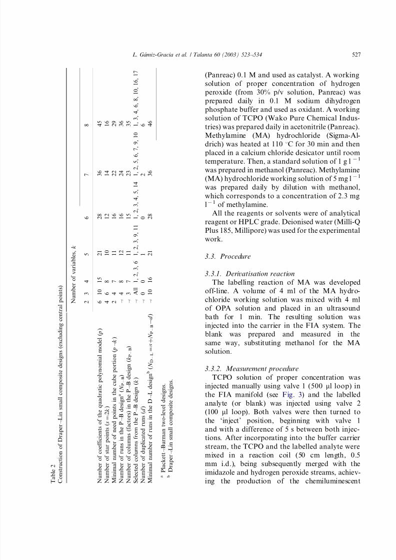
Lin small composite design (see Table 2).

In this paper, we propose the use of a Draper Á /

Lin small composite design for the optimisation of four variables (Fig. 2) that influence the CL

emission using the PO-CL system for the detection

of methylamine after derivatisation with OPA.

The quadratic equation for four variables includes

15 coefficients (an independent term, four quad-

ratic terms, four linear terms and six interaction

terms). Considering that the number of star-points

needed is 8 (twice than the number of variables), at

least seven points are required for the cube-portion

of the design.

From a two-level Plackett Á /Burman design witheight experiments (for seven variables), the col-

umns 1, 2, 3 and 6, are selected, removing the three

others (columns 4, 5 and 7), and obtaining a two-

level design for four variables. This design does

not show any replicated row and so, the cube-

portion is constructed with the eight experiments.

The corresponding star-points are adding to this

design (with a0/1.414), which is completed with

two central points (in order to maintain the

orthogonal condition).

Considering that these designs are currently

implemented in some statistical software [24],

they could be easily applied for optimisation

purposes in Analytical Chemistry.

3. Experimental

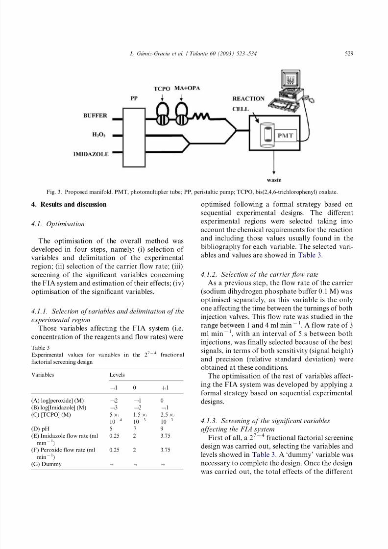
3.1. Apparatus

CL measurements were carried out on a Jasco

CL 1525 detector (Jasco Corporation), equipped

with a PTFE spiral detection cell, data control and

acquisition programme. Two Gilson Minipulse-3

(Gilson) peristaltic pumps, two Rheodyne 5020

manual injection valves (Rheodyne, L.P.), and

Omnifit tubing and connections were used for

constructing the FIA manifold in Fig. 3 [25].

3.2. Chemicals

A 500 mg l(1 OPA solution (Sigma-Aldrich)

was prepared weekly by adding 0.05 g of OPA, 1

ml methanol (Panreac), 5 ml borate buffer 0.1 M,

pH 9.0 (Sigma-Aldrich) and 0.1 ml of 2-mercap-

toethanol (Sigma-Aldrich Quımica S.A.) to a 100

ml volumetric flask, diluting to the mark with

deionised water [26]. A 2 M stock solution of

imidazole (Sigma-Aldrich) was prepared weekly in

water and proper working solutions were prepared

daily in sodium dihydrogen phosphate buffer

Table 1

Efficiency of some composite designs excluding central points

Number of variables, k

2 3 4 5 6 7 8

Number of coefficients of the quadratic polynomial model,

p

6 10 15 21 28 36 45

Number of runs in B Á /W designsa (efficiency, fB Á W) 8 (1.33) 14 (1.40) 24 (1.60) 42 (2.00) 78 (2.79) 142 (3.94) 272 (6.04)

Number of runs in B Á /H designsb (efficiency, fB Á H) Á / Á / Á / 26 (1.24) 44 (1.57) 78 (2.17) 80 (1.77)

Number of runs in D Á /L designsc (efficiency, fD Á L) Á / 10 (1.00) 16 (1.07) 21 (1.00) 28 (1.00) 36 (1.00) 46 (1.02)

a Box Á /Wilson complete composite designs.b Box Á /Hunter fractional composite designs.c Draper Á /Lin small composite designs.


8/6/2019 1497650X


(Panreac) 0.1 M and used as catalyst. A working

solution of proper concentration of hydrogen

peroxide (from 30% p/v solution, Panreac) was

prepared daily in 0.1 M sodium dihydrogenphosphate buffer and used as oxidant. A working

solution of TCPO (Wako Pure Chemical Indus-

tries) was prepared daily in acetonitrile (Panreac).

Methylamine (MA) hydrochloride (Sigma-Al-

drich) was heated at 110 8C for 30 min and then

placed in a calcium chloride desicator until room

temperature. Then, a standard solution of 1 g l(1

was prepared in methanol (Panreac). Methylamine

(MA) hydrochloride working solution of 5 mg l(1

was prepared daily by dilution with methanol,

which corresponds to a concentration of 2.3 mgl(1 of methylamine.

All the reagents or solvents were of analytical

reagent or HPLC grade. Deionised water (Milli-Q

Plus 185, Millipore) was used for the experimental

work.

3.3. Procedure

3.3.1. Deri vatisation reaction

The labelling reaction of MA was developed

off-line. A volume of 4 ml of the MA hydro-chloride working solution was mixed with 4 ml

of OPA solution and placed in an ultrasound

bath for 1 min. The resulting solution was

injected into the carrier in the FIA system. The

blank was prepared and measured in the

same way, substituting methanol for the MA

solution.

3.3.2. Measurement procedure

TCPO solution of proper concentration was

injected manually using valve 1 (500 ml loop) in

the FIA manifold (see Fig. 3) and the labelledanalyte (or blank) was injected using valve 2

(100 ml loop). Both valves were then turned to

the ‘inject’ position, beginning with valve 1

and with a difference of 5 s between both injec-

tions. After incorporating into the buffer carrier

stream, the TCPO and the labelled analyte were

mixed in a reaction coil (50 cm length, 0.5

mm i.d.), being subsequently merged with the

imidazole and hydrogen peroxide streams, achiev-

ing the production of the chemiluminescent T a b l e 2

C o n s t r u c t i o n o f D r a p e r Á / L

i n s m a l l c o m p o s i t e d e s i g n s ( e x c l u d i n g c e n t r a l p o i n

t s )

N u m

b e r o f v a r i a b l e s , k

2 3

4

5

6

7

8

N u m b e r o f c o e f f i c i e n t s o f t h e q u a d r a

t i c p o l y n o m i a l m o d e l ( p )

6 1

0

1 5

2 1

2 8

3 6

4 5

N u m b e r o f s t a r p o i n t s ( s 0 / 2 k )

4 6

8

1 0

1 2

1 4

1 6

M i n i m a l n u m b e r o f n e e d p o i n t s i n t h

e c u b e p o r t i o n ( p Á / k

)

2 4

7

1 1

1 6

2 2

2 9

N u m b e r o f r u n s i n t h e P Á / B

d e s i g n a ( N P Á

B )

Á / 4

8

1 2

1 6

2 4

3 6

N u m b e r o f c o l u m n s ( f a c t o r s ) i n t h e P

Á / B

d e s i g n ( k P Á

B )

Á / 3

7

1 1

1 5

2 3

3 5

S e l e c t e d c o l u m n s f r o m t h e P Á / B

d e s i g

n ( k )

Á / A

l l 1 ,

2 ,

3 ,

6

1 ,

2 ,

3 ,

9 ,

1 1

1 ,

2 ,

3 , 4 ,

5 ,

1 4

1 ,

2 ,

5 ,

6 ,

7 ,

9 ,

1 0

1 ,

3 ,

4 ,

6 , 8 ,

1 0 ,

1 6 ,

1 7

N u m b e r o f d u p l i c a t e d r u n s ( d )

Á / 0

0

1

0

2

6

M i n i m a l n u m b e r o f r u n s i n t h e D Á / L

d e s i g n

b

( N D

Á

L 0 / s ' / N P Á B ( / d

)

Á / 1

0

1 6

2 1

2 8

3 6

4 6

a

P l a c k e t t Á / B u r m a n t w o - l e v e l d e s i g

n s .

b

D r a p e r Á / L

i n s m a l l c o m p o s i t e d e s

i g n s .


8/6/2019 1497650X


emission in the detection cell just in front of the

photomultiplier. All the testing solutions (blank

and solutions containing the derivatives of MA

with OPA) were injected by triplicate. The net

signal was then calculated as the difference be-

tween the average height from the signals corre-

sponding to the MA solution and those

corresponding to the blank.

Fig. 2. Construction of an orthogonal 18-run (four-variables) Draper Á /Lin small composite designs (used in the experimental

optimisation study of this paper) from an eight-run (seven-variables) two-level Plackett Á /Burman design.


8/6/2019 1497650X


4. Results and discussion

4.1. Optimisation

The optimisation of the overall method was

developed in four steps, namely: (i) selection of

variables and delimitation of the experimental

region; (ii) selection of the carrier flow rate; (iii)

screening of the significant variables concerning

the FIA system and estimation of their effects; (iv)

optimisation of the significant variables.

4.1.1. Selection of variables and delimitation of the

experimental region

Those variables affecting the FIA system (i.e.

concentration of the reagents and flow rates) were

optimised following a formal strategy based on

sequential experimental designs. The different

experimental regions were selected taking into

account the chemical requirements for the reaction

and including those values usually found in the

bibliography for each variable. The selected vari-

ables and values are showed in Table 3.

4.1.2. Selection of the carrier flow rate

As a previous step, the flow rate of the carrier

(sodium dihydrogen phosphate buffer 0.1 M) wasoptimised separately, as this variable is the only

one affecting the time between the turnings of both

injection valves. This flow rate was studied in the

range between 1 and 4 ml min(1. A flow rate of 3

ml min(1, with an interval of 5 s between both

injections, was finally selected because of the best

signals, in terms of both sensitivity (signal height)

and precision (relative standard deviation) were

obtained at these conditions.

The optimisation of the rest of variables affect-

ing the FIA system was developed by applying aformal strategy based on sequential experimental

designs.

4.1.3. Screening of the significant variables

affecting the FIA system

First of all, a 27(4 fractional factorial screening

design was carried out, selecting the variables and

levels showed in Table 3. A ‘dummy’ variable was

necessary to complete the design. Once the design

was carried out, the total effects of the different

Fig. 3. Proposed manifold. PMT, photomultiplier tube; PP, peristaltic pump; TCPO, bis(2,4,6-trichlorophenyl) oxalate.

Table 3

Experimental values for variables in the 27(4 fractional

factorial screening design

Variables Levels

(/1 0 '/1

(A) log[peroxide] (M) (/2 (/1 0

(B) log[Imidazole] (M) (/3 (/2 (/1

(C) [TCPO] (M) 5)/

10(4

1.5)/

10(3

2.5)/

10(3

(D) pH 5 7 9

(E) Imidazole flow rate (ml

min(1)

0.25 2 3.75

(F) Peroxide flow rate (ml

min(1)

0.25 2 3.75

(G) Dummy Á / Á / Á /


8/6/2019 1497650X


variables as well as their second order interactions

were evaluated considering the corresponding total

effect estimated, shown in Table 4.

4.1.3.1. Effect of main variables. All those vari-

ables (and confounded second order interactions)

whose total effect estimated was lower than 5% of

the absolute value of the highest effect (which

corresponds to the total effect of peroxide flow

rate, that is 737.51)/0.050/36.88) were considered

as non-significant. Thus, TCPO concentration,

imidazole flow rate and second order interactions,

which are confounded with them (see Table 4)

were considered as non significant variables and

the values corresponding to their ‘0 level’ were

selected for subsequent studies, except in the case

of TCPO concentration, where a concentration of

1)/10(3 M was selected, as higher concentrations

produced precipitation.

4.1.3.2. Second order interaction effects. In the

previous screening study, the total effect of eachvariable is confounded with second order interac-

tions of the rest of the variables. In the case of the

peroxide flow rate (F), the effect is confounded

with the second order interactions, log[imidazole] Á /

[TCPO] (BC) and pH-imidazole flow rate (DE). As

the variables C and E were considered as non-

significant, their second order interactions were

also considered non significant, so the total effect

estimated was due to the effect of the main

variable, that is the peroxide flow rate. For the

purpose of elucidating if the total effect of the

other variables considered as significant was due to

the variable itself or to second order interactions, a

deeper study of the effects was carried out. In thissense, an univariate study of the significant vari-

ables (namely: log[imidazole], log[peroxide] and

pH) was carried out, which consisted of measuring

the CL signal at three different levels for each

variable (see Table 3), keeping the rest of the

variables constant at the ‘0 level’. The main sided

effects were then calculated as:

Sided-up effects: variation in the response when

the value of the studied variable is changed

from the ‘0’ to the ‘'/1’ level:E (')0 y('1)( y(0):

Sided-down effects: variation in the response

when the value of the studied variable is

changed from the ‘0’ to the ‘(/1’ level:

E (()0 y((1)( y(0):

where y ('/1), y ((/1) and y (0) are the response

when the variable is in the'/

1,(/

1 and 0 level,respectively. Thus, the main total effects were

calculated as:

E 0E ('1)'E ((1)

The estimated effects are shown in Table 5.

Those sided effects are both deviations that are

caused by logarithmic changes of the unit from the

zero value (that is, a factor of ten in concentration

up and down). These differences in the concentra-

tion could explain why the sided-up and sided-

down effects are so different.

Table 4

Estimated effects for the variables affecting the CL signal (from

a 27(4 fractional factorial screening design)

Variable Total effecta Significant

(A) log[peroxide]'/BD'/CE 52 Yes

(B) log[imidazole]'/AD'/CF (/103 Yes

(C) [TCPO]'/AE'/BF (/19 Non

(D) pH'/AB'/EF (/49 Yes

(E) Imidazole flow rate'/AC'/DF (/35 Non

(F) Peroxide flow rate'/BC'/DE (/738 Yes

(G) Dummy'/AF'/BE'/CD 37 Yes

Standard deviations, S.D., are based on pure error with 2

degrees of freedom. (Effects and S.D. are expressed in arbitrary

units of the CL signal).a

Standard deviation0/9/12.8.

Table 5

Estimated effects for significant variables confounded with

second order interactions (univariate study)

Variable Positive effect Negative effect Total effect

(A) log[peroxide] (/587 106 (/481

(B) log[imidazole] (/241 119 (/122

(D) pH (/149 363 214

Effects and S.D. are expressed in arbitrary units of the CL

signal.


8/6/2019 1497650X


Once the main total effect of the significant

variables has been estimated, the effects of the

second order interactions are estimated too, as the

difference between the total effect obtained fromthe screening design and that one obtained from

the single study of each significant variable. At this

point it must be remembered that the second order

interactions AE, BF, AC and DF were considered

as non-significant in the screening design. Also, the

significance of the ‘dummy’ variable indicates that

at least, one of the second order interactions

confounded with this variable (AF'/BE'/CD) is

significant. The obtained results for the remaining

second order interactions are shown in Table 6.

Following the same criteria than in the case of the main studied variables, those second order

interactions whose estimated total effect is lower

than 5% of the absolute value of the total effect of

peroxide flow rate, are considered as non-signifi-

cant. In this sense, the variables and interactions

finally considered as significant were: log[perox-

ide], log[imidazole], pH, peroxide flow rate, and

the second order interactions log[peroxide] Á /log[i-

midazole] (AB), log[imidazole] Á /pH (BD) and

log[peroxide] Á /peroxide flow rate (AF). These

variables were considered in the next optimisationstep.

4.1.4. Optimisation of the significant variables

The next step was the optimisation of the

significant variables, namely: log[peroxide], log[i-

midazole], pH and peroxide flow rate. With this

purpose, a Draper Á /Lin small composite design

(orthogonal), which permits the optimisation of

the variables with a minimum number of experi-

ments, was selected (see Fig. 2). The selected

experimental region is shown in Table 7. Once

the response was obtained and the data were

analysed by means of the ANOVA, those quad-

ratic coefficients whose P -value was lower than

5% were not considered in the model. These

coefficients were: AB, CD and DD. The ANOVAwas performed again and the final P -values are

shown in Table 8.

The equation of the fitted response surface was:

CL signal0502:4'105:8)A(173:1)B

(150:0)C(87:0)D(126:4)A2

(100:5)AC(261:5)AD(88:6

)B2(179:2)BC'78:0)BD

(52:7)C2

The approximated optimum scores were ob-tained from this equation. For log[Imidazole] and

peroxide flow rate these values were 0.093 and (/

1.34, respectively, which are included in the

selected experimental region (see Fig. 4). These

codified values correspond to real values of 1.2)/

10(2 M and 0.66 ml min(1, respectively. On the

other hand, the optimum values for log[peroxide]

and pH were 1.41 and (/1.41, respectively, which

are in the limit of the experimental region, and

correspond to real values of 0.54 and 5 M,

respectively.

4.1.5. Verification of the first optimum

In order to verify these optimum coordinates, a

further optimisation design was carried out in a

more limited experimental region. In this sense, a

narrow Draper Á /Lin small composite design (face-

centred) around the predicted optimum was con-

structed. The new selected experimental region is

shown in Table 9. Once the response was obtained

and the data were analysed by means of the

ANOVA, those quadratic coefficients whose P -

value was lower than 5% were removed of the

Table 6

Estimated effects for confounded second order interactions

Effect

(A) log[peroxide]'/BD'/CE0/51.59 (A) log[peroxide]0/(/481 BD0/532 CE0/NS*

(B) log[imidazole]'/AD'/CF0/(/102.91 (B) log[imidazole]0/(/122 AD0/20 (NS*) CF0/NS*

(D) pH'/AB'/EF0/(/48.84 (D) pH0/214 AB0/(/263 EF0/NS*

Effects and S.D. are expressed in arbitrary units of the CL signal.

* NS, non-significant.


8/6/2019 1497650X


model. These coefficients were: A (log[peroxide]),

B (log[imidazole]), AA, AB, BD and DD. A new

ANOVA was performed on the reduced model

and the final P -values are shown in Table 10.The equation of the final fitted response surface

was:

CL signal0858:3(112:3)C(30:6)D(16:0

)AC(114:7)AD(113:6)B2

(101:6)BC(185:7)C2

The final optimum values were obtained from

this equation. For log[Imidazole] and pH these

values were 0.29 and (/0.10, respectively, which

correspond to real values of 1.4)/10(2 M and 5.7,

respectively. On the other hand, the optimumvalues for log[peroxide] and peroxide flow rate

were 1 and (/1, respectively, which are in the limit

of the experimental region, and correspond to real

values of 0.56 M and 0.5 ml min(1, respectively.

Those values are close to those reported by the

previous Draper Á /Lin small composite design.

First and final optimum values for all optimised

variables are summarised in Table 11.

4.1.6. Influence of the methylamine concentration

on the CL signal

Once the crucial experimental variables had

been optimised and in order to check the depen-

dence of the methylamine concentration on CL

signal at these final optimum values, a study was

performed varying the concentration of MA

hydrochloride from 0.5 to 10 mg l(1, which

corresponds to values of MA in the range from0.23 to 4.6 mg l(1. The obtained response is

shown in Fig. 4. It can be stated that a linear

response can be expected up to a concentration of

approximately 1.4 mg l(1 of MA.

Table 7

Experimental values for variables in the first Draper Á /Lin small composite design (orthogonal)

Variable Level

(/1.41 (/1 0 '/1 '/1.41

log[peroxide] (M) (/1.735 (/1.5 (/1 (/0.5 (/0.265

log[imidazole] (M) (/3 (/2.71 (/2 (/1.29 (/1

pH 5 5.64 7 8.36 9

Peroxide flow rate (ml min(1) 0.53 1 2 3 3.47

Table 8

Analysis of variance (ANOVA) for CL signals obtained from the first Draper Á /Lin small composite design (orthogonal) without the

non-significant coefficients

Source Sum of squares Degrees of freedom Mean square F -ratio P -value

(A) log[peroxide] 44 748.4 1 44 748.4 467.91 0.0294

(B) log[imidazole] 119 883.0 1 119 883.0 1253.56 0.0180(C) pH 269 864.0 1 269 864.0 2821.83 0.0120

(D) Peroxide flow rate 90 883.4 1 90 883.4 950.32 0.0206

AA 127 762.0 1 127 762.0 1335.95 0.0174

AC 80 866.9 1 80 866.9 845.58 0.0219

AD 182 288.0 1 182 288.0 1906.09 0.0146

BB 62 776.4 1 62 776.4 656.42 0.0248

BC 256 922.0 1 256 922.0 2686.50 0.0123

BD 16 232.1 1 16 232.1 169.73 0.0488

CC 22 225.5 1 22 225.5 232.40 0.0417

Lack of fit 63 816.6 5 12 763.3 133.46 0.0647

Pure error 95.6344 1 95.6344


8/6/2019 1497650X


5. Conclusions

The use of the PO-CL reaction coupled to a FIA

manifold as an alternative detection system for

methylamine has been proposed. The method

implies: (i) formation of a MA-OPA derivative

(fluorophore) in presence of 2-mercaptoethanol;

(ii) oxidation of TCPO by H2O2 using imidazol as

catalyst, in presence of the fluorophore, whose CL

emission is proportional to the methylamine con-

Fig. 4. Plot for CL-signal vs. methylamine concentration (CL signal is expressed in arbitrary units).

Table 9

Experimental values for variables in the second Draper Á /Lin

small composite design (face-centred)

Variable Level

(/1 0 '/1

log[peroxide] (M) (/0.75 (/0.5 (/0.25

log[imidazole] (M) (/2.5 (/2.0 (/1.5

pH 5.0 5.75 6.5

Peroxide flow rate (ml min(1) 0.5 1.0 1.5

Table 10

Analysis of variance (ANOVA) for CL signals obtained from the second Draper Á /Lin small composite design (face-centred) without

the non-significant coefficients

Source Sum of squares Degrees of freedom Mean square F -ratio P -value

(C) pH 126 065.0 1 126 065.0 122.13 0.0001

(D) Peroxide flow rate 9374.01 1 9374.01 9.08 0.0296

AC 2059.86 1 2059.86 2.00 0.2169

AD 105 251.0 1 105 251.0 101.97 0.0002

BB 40 746.3 1 40 746.3 39.48 0.0015

BC 82 513.4 1 82 513.4 79.94 0.0003

CC 108 795.0 1 108 795.0 105.40 0.0002

CD 24 537.8 1 24 537.8 23.77 0.0046

Lack of fit 36 284.5 5 7256.91 7.03 0.0259

Pure error 5160.89 5 1032.18

Table 11

First and final optimum values for optimised variables involved

in the PO-CL Á /FIA system

Variable First opti-

mum

Final opti-

mum

Carrier flow rate (ml min(1) 3 3

[Peroxide] (M) 0.54 0.56

[Imidazole] (M) 1.2)/10(2 1.4)/10(2

[TCPO] (M) 1.0)/10(3 1.0)/10(3

pH 5.0 5.7

Peroxide flow rate (ml min(1) 0.66 0.5

Imidazole flow rate (ml

min(1)

2 2


8/6/2019 1497650X


centration. A formal strategy has been carried out

for the multidimensional optimisation of the

experimental variables of the PO-CL Á /FIA system

with the aim to determine methylamine deriva-tives. Due to the interdependence of the chemical

and operational variables, a formal strategy based

on the use of experimental designs has been

proposed for optimisation purpose. This implies

the consecution of several steps, including the use

of Draper Á /Lin small composite designs, scarcely

used in the optimisation of analytical methods.

This strategy offers interesting possibilities in the

optimisation of analytical signals from other

analytical techniques. In this sense, further re-

search is being orientated to the determination of carbamates by employing the PO-CL system,

using the new experimented strategy proposed in

this paper.

Acknowledgements

The authors are grateful to Instituto Nacional

de Investigacion y Tecnologıa Agraria y Alimen-

taria, INIA (National Institute of Agricultural and

Food Research and Technology, Ministerio deAgricultura, Pesca y Alimentacion, Spain, Project

CAL00-002-C2-1) and to the Junta de Andalucıa

(Programa de Acciones Coordinadas, 2001) for

financial support, and to Professor Norman D.

Draper for technical information on small compo-

site design.

References

[1] A.M. Garcıa-Campana, W.R.G. Baeyens, X. Zhang,

Chemiluminescence-based analysis: principles and analy-tical applications, in: A.M. Garcıa-Campana, W.R.G.

Baeyens (Eds.), Chemiluminescence in Analytical Chem-

istry, Marcel Dekker, New York, 2001.

[2] M. Valcarcel, M.D. Luque de Castro, Flow Injection

Analysis, Principles and applications, first ed, Ellis Hor-

wood, Chichester, 1987.

[3] A. Matousek de Abel de la Cruz, J.L. Burgera, M.

Burgera, C. Rivas, Talanta 42 (1995) 701 Á /709.

[4] M.M.M.B. Duarte, G.O. Neto, L.T. Kubota, J.L.L. Filho,

M.F. Pimentel, F. Lima, V. Lins, Anal. Chim. Acta 350

(1997) 353 Á /357.

[5] J.R. Luna, J.F. Ovalles, A. Leon, M. Buchheister, Frese-

nius J. Anal. Chem. 167 (2000) 201 Á /203.

[6] C. Vannecke, S. Bare, M. Bloomfield, D.L. Massart, J.

Pharm. Biomed. Anal. 18 (1999) 963 Á /973.[7] C. Vannecke, M. Bloomfield, Y. Vander Heyden, D.L.

Massart, J. Pharm. Biomed. Anal. 21 (1999) 241 Á /255.

[8] C. Vannecke, A. Nguyen Minh Nguyet, M.S. Bloomfield,

A.J. Staple, Y. Vander Heyden, D.L. Masart, J. Pharm.

Biomed. Anal. 23 (2000) 291 Á /306.

[9] C. Vannecke, E. Van Gyseghem, M.S. Bloomfield, T.

Coomber, Y. Vander Heyden, D.L. Massart, Anal. Chim.

Acta 446 (2001) 413 Á /428.

[10] C. Vannecke, M.S. Bloomfield, Y. Vander Heyden, D.L.

Massart, Anal. Chim. Acta 455 (2002) 117 Á /130.

[11] A.C. Calokerinos, L.P. Palilis, Chemiluminescence in flow

injection analysis, in: A.M. Garcıa-Campana, W.R.G.

Baeyens (Eds.), Chemiluminescence in Analytical Chem-

istry, Marcel Dekker, New York, 2001.

[12] O.M. Steijer, H.C.M. den Nieuwenboer, H. Lingeman,

U.A.T.h. Brinkman, J.J.M. Holthuis, A.K. Smilde, Anal.

Chim. Acta 320 (1996) 99 Á /105.

[13] J.C.G. Esteves da Silva, J.R.M. Dias, J.M.C.S. Magalhaes,

Anal. Chim. Acta 450 (2001) 175 Á /184.

[14] K. Imai, T. Toyo’oka, H. Miyano, Analyst 109 (1984)

1365 Á /1373.

[15] M. Stigbrand, T. Jonsson, E. Ponten, K. Irgum, Mechan-

ism and application of peroxyoxalate chemiluminescence,

in: A.M. Garcıa-Campana, W.R.G. Baeyens (Eds.), Che-

miluminescence in Analytical Chemistry, Marcel Dekker,

New York, 2001.

[16] C. Nsengiyumva, J.O. Deber, W. VandeWauw, A.J.

Vlietinck, F. Parmentier, Chromatographia 44 (1997)

634 Á /644.

[17] N.R. Draper, Technometrics 27 (1985) 173 Á /180.

[18] N.R. Draper, D.K.J. Lin, Technometrics 32 (1990) 187 Á /

194.

[19] G.E.P. Box, K.B. Wilson, J. R. Stat. Soc. Ser. B 13 (1951)

1 Á /45.

[20] G.E.P. Box, J.S. Hunter, Ann. Math. Stat. 28 (1957) 195 Á /

241.

[21] G.E.P. Box, N.R. Draper, Empirical Model-Building and

Response Surfaces, Wiley, New York, 1987, pp. 508 Á /515.

[22] R.L. Plackett, J.P. Burman, Biometrika 33 (1946) 305 Á /

325.[23] K. Jones, Int. Lab. 11 (1986) 32 Á /45.

[24] Statgraphics Plus 5.0, Statistical Graphics Corporation,

Manugistics Inc., Rockville, USA, 2000.

[25] L. Gamiz-Gracia, A.M. Garcıa-Campana, F. Ales Bar-

rero, M.A. Dorato, M. Roman Ceba, W.R.G. Baeyens,

Luminescence 17 (2002) 199 Á /201.

[26] EPA Method 531.1. Measurement of N -methylcarbamoy-

loximes and N -methylcarbamates in water by direct

aqueous injection HPLC with post column derivatisation,

Revision 3.1 (Edited 1995).


1497650X

Documents