NON-COOPERATIVE GAMES MIHAI MANEA 1. Normal-Form Games A normal (or strategic ) form game is a triplet (N,S,u) with the following properties: • N = {1, 2,...,n} is a finite set of players • S i 3 s i is the set of pure strategies of player i; S = S 1 ×···× S n 3 s =(s 1 ,...,s n ) • u i : S → R is the payoff function of player i; u =(u 1 ,...,u n ). Outcomes are interdependent. Player i ∈ N receives payoff u i (s 1 ,...,s n ) when the pure strategy profile s =(s 1 ,...,s n ) ∈ S is played. The game is finite if S is finite. We write S -i = Q j 6 =i S j 3 s -i . The structure of the game is common knoweldge : all players know (N,S,u), and know that their opponents know it, and know that their opponents know that they know, and so on. For any measurable space X we denote by Δ(X ) the set of probability measures (or distributions) on X . 1 A mixed strategy for player i is an element σ i of Δ(S i ). A mixed strategy profile σ ∈ Δ(S 1 ) ×···× Δ(S n ) specifies a mixed strategy for each player. A correlated strategy profile σ is an element of Δ(S ). A mixed strategy profile can be seen as a special case of a correlated strategy profile (by taking the product distribution), in which case it is also called independent to emphasize the absence of correlation. A correlated belief for player i is an element σ i of Δ(S i ). The set of independent beliefs for i is - - Q j 6 =i Δ(S j ). It is assumed that player i has von Neumann-Morgenstern preferences over Δ(S ) and u i extends to Δ(S ) as follows u i (σ)= X σ(s)u i (s). s∈S Date : January 19, 2017. These notes benefitted from the proofreading and editing of Gabriel Carroll. The treatment of classic topics follows Fudenberg and Tirole’s text “Game Theory” (FT). Some material is borrowed from Muhamet Yildiz. 1 In most of our applications X is either finite or a subset of a Euclidean space. Department of Economics, MIT

Welcome message from author
This document is posted to help you gain knowledge. Please leave a comment to let me know what you think about it! Share it to your friends and learn new things together.
Transcript
NON-COOPERATIVE GAMES
MIHAI MANEA
1. Normal-Form Games
A normal (or strategic) form game is a triplet (N,S, u) with the following properties:
• N = 1, 2, . . . , n is a finite set of players
• Si 3 si is the set of pure strategies of player i; S = S1 × · · · × Sn 3 s = (s1, . . . , sn)
• ui : S → R is the payoff function of player i; u = (u1, . . . , un).
Outcomes are interdependent. Player i ∈ N receives payoff ui(s1, . . . , sn) when the pure
strategy profile s = (s1, . . . , sn) ∈ S is played. The game is finite if S is finite. We write
S−i =∏
j 6=i Sj 3 s−i.
The structure of the game is common knoweldge: all players know (N,S, u), and know
that their opponents know it, and know that their opponents know that they know, and so
on.
For any measurable space X we denote by ∆(X) the set of probability measures (or
distributions) on X.1 A mixed strategy for player i is an element σi of ∆(Si). A mixed
strategy profile σ ∈ ∆(S1) × · · · × ∆(Sn) specifies a mixed strategy for each player. A
correlated strategy profile σ is an element of ∆(S). A mixed strategy profile can be seen as
a special case of a correlated strategy profile (by taking the product distribution), in which
case it is also called independent to emphasize the absence of correlation. A correlated belief
for player i is an element σ i of ∆(S i). The set of independent beliefs for i is− −∏
j 6=i ∆(Sj).
It is assumed that player i has von Neumann-Morgenstern preferences over ∆(S) and ui
extends to ∆(S) as follows
ui(σ) =∑
σ(s)ui(s).s∈S
Date: January 19, 2017.These notes benefitted from the proofreading and editing of Gabriel Carroll. The treatment of classic topicsfollows Fudenberg and Tirole’s text “Game Theory” (FT). Some material is borrowed from Muhamet Yildiz.1In most of our applications X is either finite or a subset of a Euclidean space.
Department of Economics, MIT
2 MIHAI MANEA
2. Dominated Strategies
Are there obvious predictions about how a game should be played?
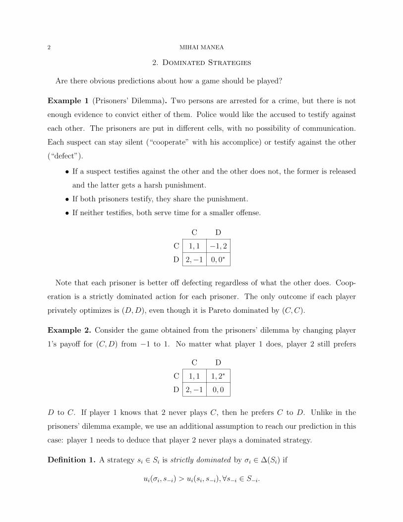
Example 1 (Prisoners’ Dilemma). Two persons are arrested for a crime, but there is not
enough evidence to convict either of them. Police would like the accused to testify against
each other. The prisoners are put in different cells, with no possibility of communication.
Each suspect can stay silent (“cooperate” with his accomplice) or testify against the other
(“defect”).
• If a suspect testifies against the other and the other does not, the former is released
and the latter gets a harsh punishment.
• If both prisoners testify, they share the punishment.
• If neither testifies, both serve time for a smaller offense.
C D
C 1, 1 −1, 2
D 2,−1 0, 0∗
Note that each prisoner is better off defecting regardless of what the other does. Coop-
eration is a strictly dominated action for each prisoner. The only outcome if each player
privately optimizes is (D,D), even though it is Pareto dominated by (C,C).
Example 2. Consider the game obtained from the prisoners’ dilemma by changing player
1’s payoff for (C,D) from −1 to 1. No matter what player 1 does, player 2 still prefers
C D
C 1, 1 1, 2∗
D 2,−1 0, 0
D to C. If player 1 knows that 2 never plays C, then he prefers C to D. Unlike in the
prisoners’ dilemma example, we use an additional assumption to reach our prediction in this
case: player 1 needs to deduce that player 2 never plays a dominated strategy.
Definition 1. A strategy si ∈ Si is strictly dominated by σi ∈ ∆(Si) if
ui(σi, s−i) > ui(si, s−i),∀s−i ∈ S−i.

NON-COOPERATIVE GAMES 3
Example 3. There are situations where a strategy is not strictly dominated by any pure
strategy, but is strictly dominated by a mixed one. For instance, in the game below B is
L R
T 3, x 0, x
M 0, x 3, x
B 1, x 1, x
strictly dominated by a 50-50 mix between T and M , but not by either T or M .
Example 4 (A Beauty Contest). Consider an n-player game in which each player announces
a number in the set 1, 2, . . . , 100 and a prize of $1 is split equally between all players whose
number is closest to 2/3 of the average of all numbers announced. Talk about the Keynesian
beauty contest.
We can iteratively eliminate dominated strategies, under the assumption that “I know
that you know that I know. . . that I know the payoffs and that no one would ever use a
dominated strategy.
Definition 2. For all i ∈ N , set S0i = Si and define Ski recursively by
Ski = si ∈ Sk−1i | 6 ∃σi ∈ ∆(Sk−1
i ), ui(σi, s i) > ui(si, s )− −i ,∀s−i ∈ Sk−1−i .
The set of pure strategies of player i that survive iterated deletion of strictly dominated
strategies is S∞ = ∩ ki k 0Si . The set of surviving mixed strategies is≥
σi ∈ ∆(Si∞)| 6 ∃σi′ ∈ ∆(Si
∞), ui(σi′, s )−i > ui(σi, s−i),∀s−i ∈ S∞−i.
Remark 1. In a finite game the elimination procedure ends in a finite number of steps, so
S∞ is simply the set of surviving strategies at the last stage.
Remark 2. In an infinite game, if S is a compact metric space and u is continuous, then
one can use Cantor’s theorem (a decreasing nested sequence of non-empty compact sets has
nonempty intersection) to show that S∞ 6= ∅.
Remark 3. The definition above assumes that at each iteration all dominated strategies of
each player are deleted simultaneously. Clearly, there are many other iterative procedures
4 MIHAI MANEA
that can be used to eliminate strictly dominated strategies. However, the limit set S∞ does
not depend on the particular way deletion proceeds.2 The intuition is that a strategy which
is dominated at some stage is dominated at any later stage.
Remark 4. The outcome does not change if we eliminate strictly dominated mixed strategies
at every step. The reason is that a strategy is dominated against all pure strategies of the
opponents if and only if it is dominated against all their mixed strategies. Eliminating mixed
strategies for player i at any stage does not affect the set of strictly dominated pure strategies
for any player j 6= i at the next stage.
2.1. Detour on common knowledge. Common knowledge looks like an innocuous as-
sumption, but may have strong consequences in some situations. Consider the following
story. Once upon a time, there was a village with 100 married couples. The women had
to pass a logic exam before being allowed to marry; thus all married women were perfect
reasoners. The high priestess was not required to take that exam, but it was common knowl-
edge that she was truthful. The village was small, so everyone would be able to hear any
shot fired in the village. The women would gossip about adulterous relationships and each
knew which of the other women’s husbands were unfaithful. However, no one would ever
inform a wife about her own cheating husband.
The high priestess knew that some husbands were unfaithful, and one day she decided
that such immorality should not be tolerated any further. This was a successful religion and
all women agreed with the views of the priestess.
The priestess convened all the women at the temple and publicly announced that the well-
being of the village had been compromised—there was at least one cheating husband. She
also pointed out that even though none of them knew whether her husband was faithful,
each woman knew about the other unfaithful husbands. She ordered each woman to shoot
her husband on the midnight of the day she was certain of his infidelity. 39 silent nights
went by and on the 40th shots were heard. How many husbands were shot? Were all the
unfaithful husbands caught? How did some wives learn of their husbands’ infidelity after 39
nights in which nothing happened?
2This property does not hold for weakly dominated strategies.
NON-COOPERATIVE GAMES 5
Since the priestess was truthful, there must have been at least one unfaithful husband in
the village. How would events have unfolded if there was exactly one unfaithful husband?
His wife, upon hearing the priestess’ statement and realizing that she does not know of any
unfaithful husband, would have concluded that her own marriage must be the only adulterous
one and would have shot her husband on the midnight of the first day. Clearly, there must
have been more than one unfaithful husband. If there had been exactly two unfaithful
husbands, then each of the two cheated wives would have initially known of exactly one
unfaithful husband, and after the first silent night would infer that there were exactly two
cheaters and her husband is one of them. (Recall that the wives were all perfect logicians.)
The unfaithful husbands would thus both be shot on the second night. As no shots were
heard on the first two nights, all women concluded that there were at least three cheating
husbands. . . Since shootings were heard on the 40th night, it must be that exactly 40 husbands
were unfaithful and they were all exposed and killed simultaneously.
3. Rationalizability
Rationalizability is a solution concept introduced independently by Bernheim (1984) and
Pearce (1984). Like iterated strict dominance, rationalizability derives restrictions on play
from common knowledge of the payoffs and of the fact that players are “reasonable” in a
certain way. Dominance: it is not reasonable to use a strategy that is strictly dominated.
Rationalizability: it is not rational for a player to choose a strategy that is not a best response
to some beliefs about his opponents’ strategies.
What is a “belief”? In Bernheim (1984) and Pearce (1984) each player i’s beliefs σ−i
about the play of j 6= i must be independent, i.e., σ i ∈ j=i ∆(S ).− 6 j Alternatively, we
may allow player i to believe that the actions of his opponen
∏ts are correlated, i.e., any
σ i ∈ ∆(S i) is a possibility. The two definitions have different implications for n 3.− − ≥
We focus on the case with correlated beliefs. It should be emphasized that such beliefs
represent a player’s uncertainty about his opponents’ actions and not his theory about their
deliberate randomization and coordination. For instance, i may place equal probability on
two scenarios: either both j and k pick action A or they both play B. If i is not sure which
theory is true, then his beliefs are correlated even though he knows that j and k are acting
independently.

6 MIHAI MANEA
Definition 3. A strategy σi ∈ Si is a best response to a belief σ−i ∈ ∆(S−i) if
ui(σi, σ−i) ≥ ui(si, σ−i),∀si ∈ Si.
We can again iteratively develop restrictions imposed by common knowledge of the payoffs
and rationality to obtain the definition of rationalizability.
Definition 4. Set S0 = S and let Sk be given recursively by
Ski = si ∈ Sk−1i |∃σ i ∈ ∆(Sk−1
− −i ), ui(si, σ i) ≥ ui(si′ , σ ,−i) ∀s′i ∈ Sk−1
− i .
The set of correlated rationalizable strategies for player i is Si∞ = k strategy≥0 S
ki . A mixed
σi ∈ ∆(Si) is rationalizable if there is a belief σ s.t.−i ∈ ∆(S∞−i)
⋂ui(σi, σ−i) ≥ ui(si, σ−i) for
all si ∈ Si∞.
The definition of independent rationalizability replaces ∆(Sk−1i ) and ∆(S∞i) above with∏ − −
j=i ∆(Sk−1j ) and
∏j=i ∆(S ely6 j
∞), respectiv .6
Example 5 (Rationalizability in Cournot duopoly). Two firms compete on the market for
a divisible homogeneous good. Each firm i = 1, 2 has zero marginal cost and simultaneously
decides to produce an amount of output qi ≥ 0. The resulting price is p = 1− q1− q2. Hence
the profit of firm i is given by qi(1− q1 − q2). The best response correspondence of firm i is
Bi(qj) = max(0, (1− qj)/2) (j = 3− i). If i knows that qj S q then Bi(qj) T (1− q)/2.
We know that q ≥ q0 = 0 for i = 1, 2. Hence q ≤ q1 = B (q0 0i i i ) = (1−q )/2 and S1
i = [0, q1]
for all i. But then q 2i ≥ q = B 1 1 2 2 1
i(q ) = (1 − q )/2 and Si = [q , q ] for all i. . . We obtain a
sequence
q0 ≤ q2 ≤ . . . ≤ q2k ≤ . . . ≤ qi ≤ . . . ≤ q2k+1 ≤ . . . ≤ q1,
where q2k =∑k 1/4l = (1 − 1/4k)/3 and q2k+1 k
l = 2=1 (1 − q )/2 for all k ≥ 0 such that
Ski = [qk−1, qk] for k odd and Ski = [qk, qk−1] for k even. Clearly, limk qk = 1/3, hence the→∞
only rationalizable strategy for firm i is qi = 1/3. This is also the unique Nash equilibrium,
which we define next. What are the rationalizable strategies when there are more than two
firms?
We say that a strategy σi is never a best response for player i if it is not a best response
to any σ i ∈ ∆(S i). Recall that a strategy σi of player i is strictly dominated if there exists− −
σi′ ∈ ∆(Si) s.t. ui(σi
′, s−i) > ui(σi, s i), ∀s .− i ∈ S− −i
NON-COOPERATIVE GAMES 7
Theorem 1. In a finite game, a strategy is never a best response if and only if it is strictly
dominated.
Proof. Clearly, a strategy σi strictly dominated for player i by some σi′ cannot be a best
response for any belief σ i ∈ ∆(S i) as σi′ yields a strictly higher payoff than σi against any− −
such σ .−i
We are left to show that a strategy which is never a best response must be strictly domi-
nated. We prove that any strategy σi of player i which is not strictly dominated must be a
best response for some beliefs. Define the set of “dominated payoffs” for i by
D = x ∈ RS−i|∃σi ∈ ∆(Si), x ≤ ui(σi, ·).
Clearly D is non-empty, closed and convex. Also, ui(σi, ·) does not belong to the interior of
D because it is not strictly dominated by any σi ∈ ∆(Si). By the supporting hyperplane
theorem, there exists α ∈ RS−i different from the zero vector s.t. α ·ui(σi, ·) ≥ α ·x,∀x ∈ D.
In particular, α · ui(σi, ·) ≥ α · ui(σi, ·),∀σi ∈ ∆(Si). Since D is not bounded from below,
each component of α needs to be non-negative. We can normalize α so that its components
sum to 1, in which case it can be interpreted as a belief in ∆(S−i) with the property that
ui(σi, α) ≥ ui(σi, α),∀σi ∈ ∆(Si). Thus σi is a best response to α.
Corollary 1. Correlated rationalizability and iterated strict dominance coincide.
Theorem 2. For every k ≥ 0, each si ∈ Ski is a best response (within Si) to a belief in
∆(Sk−1i ).−
Proof. Fix si ∈ Ski . We know that si is a best response within Sk−1i to some σ−i ∈ ∆(Sk−1
−i ).
If si was not a best response within Si to σ i, let s′i be such a best response. Since s− i is a
best response within Sk−1i to σ i, and s′i is a strictly better response than si to σ i, we need− −
s′i ∈/ Sk−1i . Then s′i was deleted at some step of the iteration, say s′i ∈ Sl−1
i but s′i ∈/ Sli for
some l ≤ k − 1. This contradicts the fact that s′i is a best response in Sl−1i to σ−i, which
belongs to ∆(Sk−1i ) ⊆ ∆(Sl−1− −i ).
Corollary 2. If the game is finite, then each si ∈ Si∞ is a best response (within Si) to a
belief in ∆(S∞−i).
8 MIHAI MANEA
Definition 5. A set Z = Z1 × . . . × Zn with Zi ⊆ Si for i ∈ N is closed under rational
behavior if, for all i, every strategy in Zi is a best response to a belief in ∆(Z−i).
Theorem 3. If the game is finite (or if S is a compact metric space and u is continuous),
then S∞ is the largest set closed under rational behavior.
Proof. Clearly, S∞ is closed under rational behavior by Corollary ??. Suppose that there
exists Z1 × . . . × Zn 6⊂ S∞ that is closed under rational behavior. Consider the smallest k
for which there is an i such that Z 6⊂ Sk ⊂ ki i . It must be that k ≥ 1 and Z i S −1
− −i . By
assumption, every element in Zi is a best response to an element of ∆(Z i) ⊂ ∆(Sk−1),− −i
contradicting Zi 6⊂ Ski .
Rationalizability has strong epistemic foundations—it characterizes the strategic implica-
tions of common knowledge of rationality (see next section). As we will see later, it also has
some evolutionary foundations. In any adaptive process the proportion of players who play
a non-rationalizable strategy vanishes as the system evolves.
4. Common Knowledge of Rationality and Rationalizability
We now formalize the idea of common knowledge and show that rationalizability captures
the idea of common knowledge of rationality (and payoffs) precisely.3 We first introduce the
notion of an incomplete-information epistemic model.
Definition 6. (Information Structure) An information (or belief) structure is a list (Ω, (Ii)i N , (p )∈ i i∈N)
where
• Ω is a finite state space;
• Ii : Ω→ 2Ω is a partition of Ω for each i ∈ N such that Ii(ω) is the set of states that i
thinks are possible when the true state is ω; it assumed that ω′ ∈ Ii(ω)⇔ ω ∈ Ii(ω′);
• pi,Ii(ω) is a probability distribution on Ii(ω) representing i’s belief at ω.
The state ω summarizes all the relevant facts about the world. Note that only one of
the state is the true state of the world; all others are hypothetical states needed to encode
players’ beliefs. In state ω, player i is informed that the state is in Ii(ω) and gets no other
information. Such an information structure arises if each player observes a state-dependent
3This section builds of notes by Muhamet Yildiz.
NON-COOPERATIVE GAMES 9
signal, where Ii(ω) is the set of states for which player i’s signal is identical to the signal at
state ω. The next definition formalizes the idea that Ii summarizes all of the information of
i.
Definition 7. For any event F ⊆ Ω, player i knows at ω that F obtains if Ii(ω) ⊆ F . The
event that i knows F is
Ki(F ) = ω|Ii(ω) ⊆ F.
The event that everyone knows F is defined by
K(F ) = ∩i∈NKi(F ).
Let K0(F ) = F and Kt+1(F ) = K(Kt(F )) for t ≥ 0. Set K∞(F ) = tt 0 K (F ). K∞(F ) is≥
the set of states where F is common knowledge.
⋂
Note that K(K∞(F )) = K∞(F ). This leads to an alternative definition of common
knowledge. An event F ′ is public if F ′ = ∪ω′ F ′Ii(ω′) for all i, which is equivalent to∈
K(F ′) = F ′ (and K∞(F ′) = F ′). Then an event F is common knowledge at ω if and only if
there exists a public event F ′ with ω ∈ F ′ ⊆ F .
We have so far considered an abstract information structure for the players in N . Fix a
game (N,S, u). In order to give strategic meaning to the states, we also need to describe
what players play at each state by introducing a strategy profile s : Ω→ S.
Definition 8. A strategy profile s : Ω→ S is adapted with respect to (Ω, (Ii)i∈N , (pi)i∈N) if
si(ω) = si(ω′) whenever Ii(ω) = Ii(ω
′).
Players must choose a constant action at all states in each information set since they
cannot distinguish between states in the same information set.
Definition 9. An epistemic model (Ω, (Ii)i N , (pi)i N , s) consists of an information structure∈ ∈
and an adapted strategy profile.
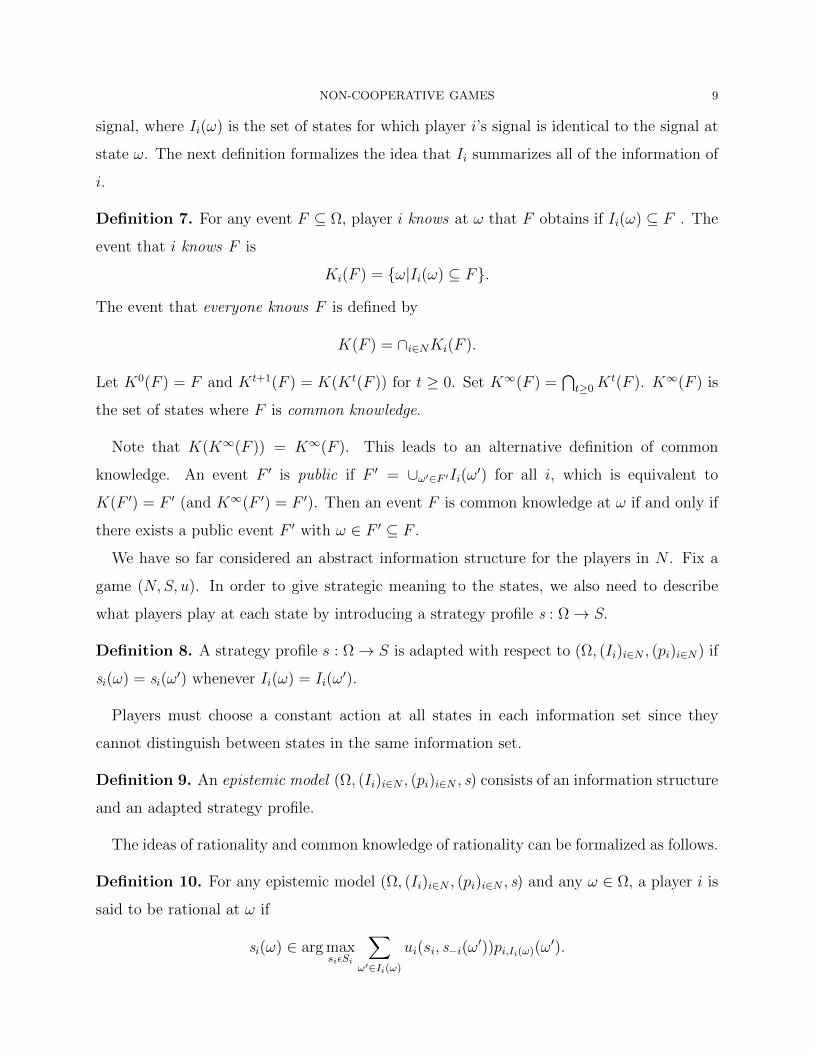
The ideas of rationality and common knowledge of rationality can be formalized as follows.
Definition 10. For any epistemic model (Ω, (Ii)i N , (pi)i N , s) and any ω ∈ Ω, a player i is∈ ∈
said to be rational at ω if
si(ω) ∈ arg max∑
ui(si, s i(ω′))pi,Ii(ω)(ω
′).siεSi
−ω′∈Ii(ω)
10 MIHAI MANEA
Definition 11. A strategy si ∈ Si consistent with common knowledge of rationality if there
exists a model (Ω, (Ij)j∈N , (pj)j N , s) and state ω∗ ∈ Ω with si(ω∗) = s at∈ i which it is
common knowledge that all players are rational (i.e., the event R := ω ∈ Ω|every player i ∈
N is rational at ω is common knowledge at ω∗).
Given the alternative definition of common knowledge in terms of public events, si ∈
Si consistent with common knowledge of rationality if there exists an epistemic model
(Ω′, (Ij)j N , (pj)j N , s) such that sj(ω) is a best response to s j at each ω∈ ∈ − ∈ Ω for every
player j ∈ N (simply consider the restriction of the original model to Ω′ = K∞(R)). The
next result states that rationalizability is equivalent to common knowledge of rationality in
the sense that Si∞ is the set of strategies that are consistent with common knowledge of
rationality.
Theorem 4. For any i ∈ N and si ∈ Si, the strategy si is consistent with common knowledge
of rationality if and only if si is rationalizable, i.e., si ∈ Si∞.
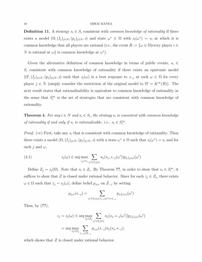
Proof. (⇒) First, take any si that is consistent with common knowledge of rationality. Then
there exists a model (Ω, (Ij)j N , (pj)j N , s) with a state ω∗ ∈ Ω such that s∈ ∈ i(ω∗) = si and for
each j and ω,
(4.1) sj(ω) ∈ arg max∑
uj(sj, s−j(ω′))pj,Ij(ω)(ω
′)sj∈Sj ω′∈Ij(ω)
Define Zj = sj(Ω). Note that si ∈ Zi. By Theorem ??, in order to show that si ∈ Si∞, it
suffices to show that Z is closed under rational behavior. Since for each zj ∈ Zj, there exists
ω ∈ Ω such that zj = sj(ω), define belief µj,ω on Z−j by setting
µj,ω(s−j) =∑
pj,Ij(ω)(ω′)
ω′∈Ij(ω),s−j(ω′)=s−j
Then, by (??),
zj = sj(ω) ∈ arg max∑
uj(sj, s−j(ω′))pj,I
sj∈j(ω)(ω
′)Sjω′∈Ij(ω)
= arg max∑
µj,ω(s j)uj(sj, s j),sj
− −∈Sj
s−j∈Z−j
which shows that Z is closed under rational behavior.
NON-COOPERATIVE GAMES 11
(⇐) Conversely, since S∞ is closed under rational behavior, for every si ∈ Si∞, there exists
a probability distribution µi,si on S∞i against which si is a best response. Define the model−
(S∞, (Ii)i∈N , (pi)i ,∈N s) with
Ii(s) = si × S∞−i
pi,s(s′) = µi,si s′−i
s(s) = s.
( )
In this model it is common knowledge that every player is rational. Indeed, for all s ∈ S∞,
si(s) = si ∈ arg max∑
ui (si′ , s i)µi,s
(s′ i)
= arg max ui (s , s i) p )s′i∈Si
− − i′
i,s(s′ .
s′∈ ∞ i∈Si
−s i S i s′− −
∑∈Ii(s)
For every si ∈ Si∞, there exists s = (si, s i) ∈ S∞ such that s− i(s) = si, showing that si is
consistent with common knowledge of rationality.
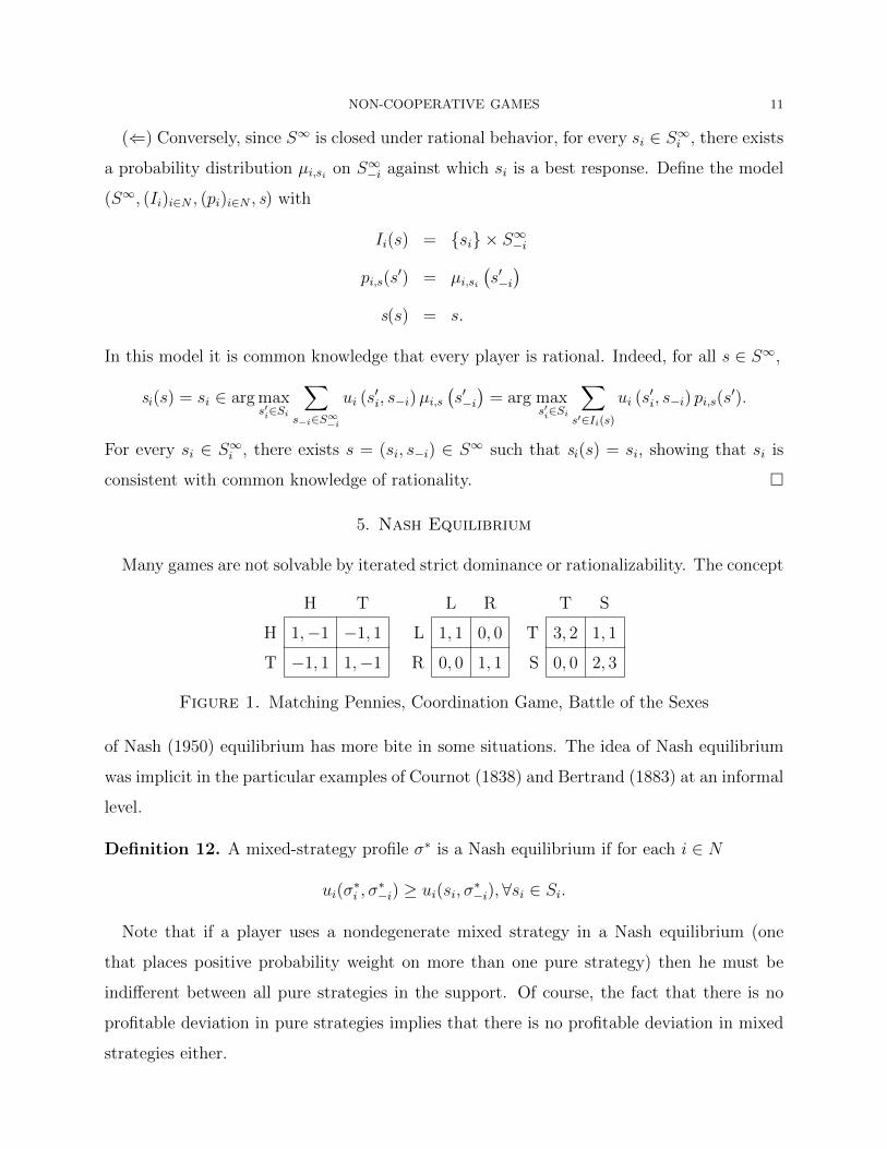
5. Nash Equilibrium
Many games are not solvable by iterated strict dominance or rationalizability. The concept
H T
H 1,−1 −1, 1
T −1, 1 1,−1
L R
L 1, 1 0, 0
R 0, 0 1, 1
T S
T 3, 2 1, 1
S 0, 0 2, 3
Figure 1. Matching Pennies, Coordination Game, Battle of the Sexes
of Nash (1950) equilibrium has more bite in some situations. The idea of Nash equilibrium
was implicit in the particular examples of Cournot (1838) and Bertrand (1883) at an informal
level.
Definition 12. A mixed-strategy profile σ∗ is a Nash equilibrium if for each i ∈ N
ui(σi∗, σ∗−i) ≥ ui(si, σ
∗ ), s S .−i ∀ i ∈ i
Note that if a player uses a nondegenerate mixed strategy in a Nash equilibrium (one
that places positive probability weight on more than one pure strategy) then he must be
indifferent between all pure strategies in the support. Of course, the fact that there is no
profitable deviation in pure strategies implies that there is no profitable deviation in mixed
strategies either.
12 MIHAI MANEA
Example 6 (Matching Pennies). This simple game shows that there may sometimes not be
any equilibria in pure strategies. We will establish that equilibria in mixed strategies exist
H T
H 1,−1 −1, 1
T −1, 1 1,−1
for any finite game.
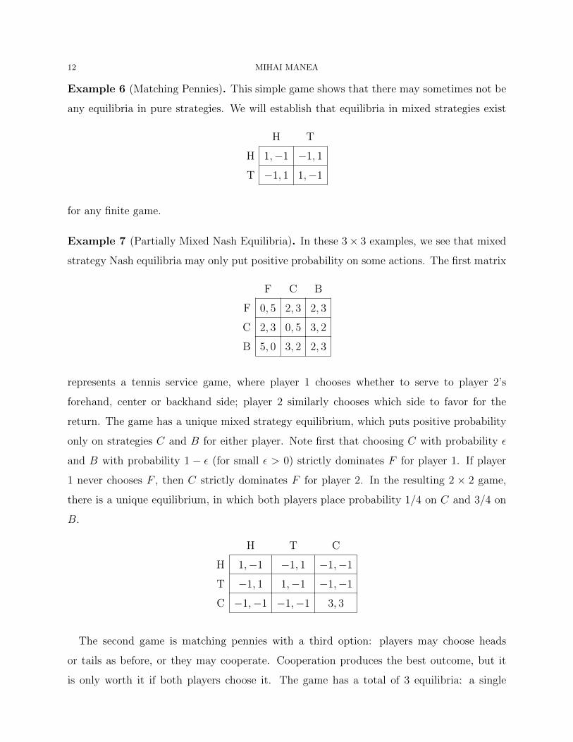
Example 7 (Partially Mixed Nash Equilibria). In these 3× 3 examples, we see that mixed
strategy Nash equilibria may only put positive probability on some actions. The first matrix
F C B
F 0, 5 2, 3 2, 3
C 2, 3 0, 5 3, 2
B 5, 0 3, 2 2, 3
represents a tennis service game, where player 1 chooses whether to serve to player 2’s
forehand, center or backhand side; player 2 similarly chooses which side to favor for the
return. The game has a unique mixed strategy equilibrium, which puts positive probability
only on strategies C and B for either player. Note first that choosing C with probability ε
and B with probability 1 − ε (for small ε > 0) strictly dominates F for player 1. If player
1 never chooses F , then C strictly dominates F for player 2. In the resulting 2 × 2 game,
there is a unique equilibrium, in which both players place probability 1/4 on C and 3/4 on
B.
H T C
H 1,−1 −1, 1 −1,−1
T −1, 1 1,−1 −1,−1
C −1,−1 −1,−1 3, 3
The second game is matching pennies with a third option: players may choose heads
or tails as before, or they may cooperate. Cooperation produces the best outcome, but it
is only worth it if both players choose it. The game has a total of 3 equilibria: a single
NON-COOPERATIVE GAMES 13
pure strategy equilibrium (C,C), where players cooperate and ignore the matching pen-
nies game; a partially mixed equilibrium ((1/2, 1/2, 0), (1/2, 1/2, 0)) where players play the
matching pennies game and ignore the option of cooperating; and a totally mixed equilibrium
((2/5, 2/5, 1/5), (2/5, 2/5, 1/5)).
To show that these are the only equilibria, we can proceed as follows: first, if player 1 is
mixing between H, T and C, he must be indifferent among all three actions, which implies
that player 2 is also mixing between H, T and C; then we can calculate the equilibrium
probabilities for the totally mixed equilibrium. If 1 is mixing between H and T (but not C)
then 2 must be mixing between H and T for this to be optimal, and 2 will never want to
play C since 1 never does. This leads to the partially mixed equilibrium. If 1 mixes between
H and C (but not T ), then 2 may only play T and C, but then 1 will never want to play
H, a contradiction; so there are no equilibria of this form (the case where 1 mixes between
T and C is analogous). Finally we check that the only pure equilibrium is (C,C).
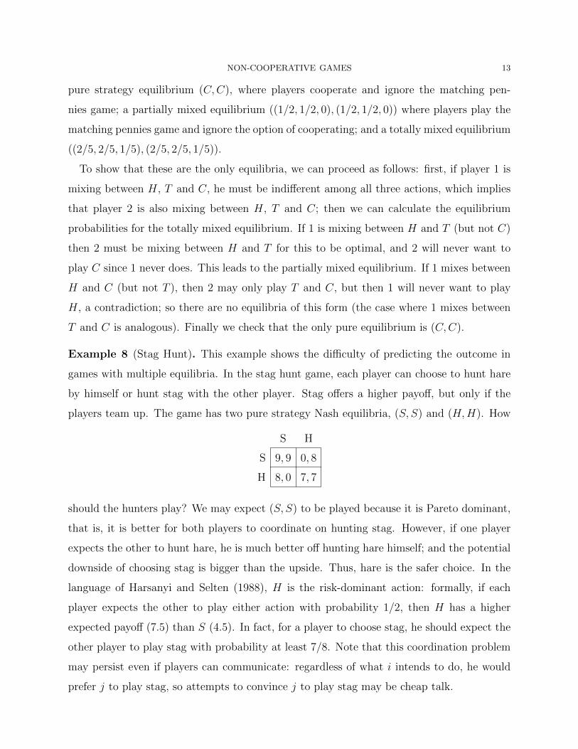
Example 8 (Stag Hunt). This example shows the difficulty of predicting the outcome in
games with multiple equilibria. In the stag hunt game, each player can choose to hunt hare
by himself or hunt stag with the other player. Stag offers a higher payoff, but only if the
players team up. The game has two pure strategy Nash equilibria, (S, S) and (H,H). How
S H
S 9, 9 0, 8
H 8, 0 7, 7
should the hunters play? We may expect (S, S) to be played because it is Pareto dominant,
that is, it is better for both players to coordinate on hunting stag. However, if one player
expects the other to hunt hare, he is much better off hunting hare himself; and the potential
downside of choosing stag is bigger than the upside. Thus, hare is the safer choice. In the
language of Harsanyi and Selten (1988), H is the risk-dominant action: formally, if each
player expects the other to play either action with probability 1/2, then H has a higher
expected payoff (7.5) than S (4.5). In fact, for a player to choose stag, he should expect the
other player to play stag with probability at least 7/8. Note that this coordination problem
may persist even if players can communicate: regardless of what i intends to do, he would
prefer j to play stag, so attempts to convince j to play stag may be cheap talk.
14 MIHAI MANEA
Nash equilibria are “consistent” predictions of how the game will be played—if all players
expect that a specific Nash equilibrium will arise then no player has incentives to play dif-
ferently. Each player must have a correct “conjecture” about the strategies of his opponents
and play a best response to his conjecture.
Formally, Aumann and Brandenburger (1995) provide a framework that can be used to
examine the epistemic foundations of Nash equilibrium. The primitive of their model is an
interactive belief system in which there is a possible set of types for each player; each type
has associated to it a payoff for every action profile, a choice of which action to play, and
a belief about the types of the other players. Aumann and Brandenburger show that in
a 2-player game, if the game being played (i.e., both payoff functions), the rationality of
the players, and their conjectures are all mutually known, then the conjectures constitute a
(mixed strategy) Nash equilibrium. Thus common knowledge plays no role in the 2-player
case. However, for games with more than 2 players, we need to assume additionally that
players have a common prior and that conjectures are commonly known. This ensures that
any two players have identical and separable (i.e., independent) conjectures about other
players, consistent with a (common) mixed strategy profile.
It is easy to show that every Nash equilibrium is rationalizable (e.g., by applying Theorem
?? to the strategies played with positive probability). The converse is not true. For example,
in the battle of the sexes (S, T ) is not a Nash equilibrium, but both S and T are rationalizable
for either player. Of course, these strategies correspond to some Nash equilibria, but one
can easily construct a game in which some rationalizable strategies do not correspond to any
Nash equilibrium.
So far, we have motivated our solution concepts by presuming that players make predic-
tions about their opponents’ play by introspection and deduction, using knowledge of their
opponents’ payoffs, knowledge that the opponents are rational, knowledge about this knowl-
edge. . . Alternatively, we may assume that players extrapolate from past observations of play
in “similar” games, with either current opponents or “similar” ones. They form expecta-
tions about future play based on past observations and adjust their actions to maximize
their current payoffs with respect to these expectations.
The idea of using adjustment processes to model learning originates with Cournot (1838).
He considered the game in Example ??, and suggested that players take turns setting their
NON-COOPERATIVE GAMES 15
outputs, each player choosing a best response to the opponent’s last-period action. Alterna-
tively, we can assume simultaneous belief updating, best responding to sample average play,
populations of players being anonymously matched, etc. In the latter context, mixed strate-
gies can also be interpreted as the proportion of players playing various strategies. If the
process converges to a particular steady state, then the steady state is a Nash equilibrium.
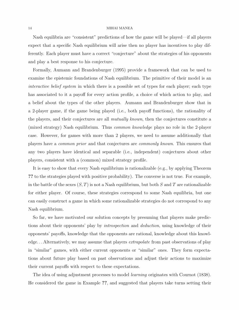
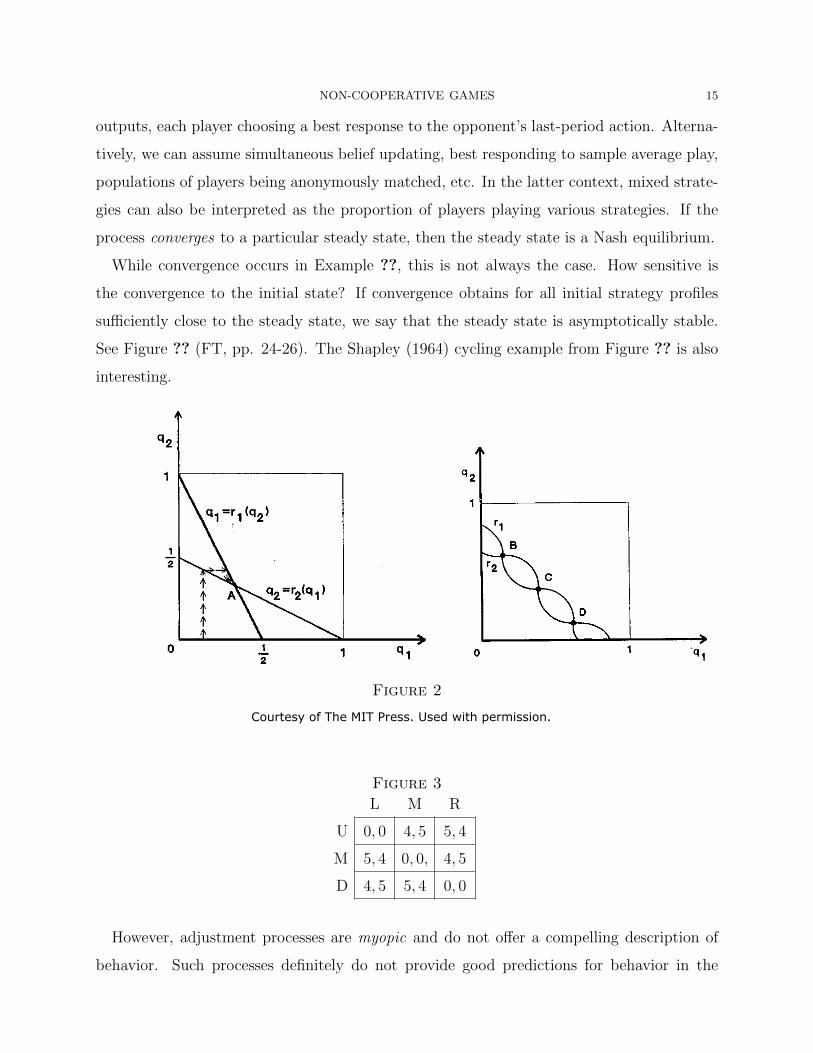
While convergence occurs in Example ??, this is not always the case. How sensitive is
the convergence to the initial state? If convergence obtains for all initial strategy profiles
sufficiently close to the steady state, we say that the steady state is asymptotically stable.
See Figure ?? (FT, pp. 24-26). The Shapley (1964) cycling example from Figure ?? is also
interesting.
Figure 2
Figure 3
L M R
U 0, 0 4, 5 5, 4
M 5, 4 0, 0, 4, 5
D 4, 5 5, 4 0, 0
However, adjustment processes are myopic and do not offer a compelling description of
behavior. Such processes definitely do not provide good predictions for behavior in the
Courtesy of The MIT Press. Used with permission.
16 MIHAI MANEA
actual repeated game, if players care about play in future periods and realize that their
current actions can affect opponents’ future play.
6. Existence and Continuity of Nash Equilibria
We can show that a Nash equilibrium exists under broad regularity conditions on strategy
spaces and payoff functions.4 Some continuity and compactness assumptions are indispens-
able because they are usually needed for the existence of solutions to (single agent) optimiza-
tion problems. Convexity is usually required for fixed-point theorems, such as Kakutani’s.5
Nash used Kakutani’s fixed point theorem to show the existence of mixed strategy equilibria
in finite games. We provide a generalization of his existence result. We start with some
mathematical background.
6.1. Topology Prerequisites. Consider two topological vector spaces X and Y . A corre-
spondence F : X ⇒ Y is a set valued function taking elements x ∈ X into subsets F (x) ⊆ Y .
The graph of F is defined by G(F ) = (x, y) |y ∈ F (x). A point x ∈ X is a fixed point
of F if x ∈ F (x). A correspondence F is non-empty/closed-valued/convex-valued if F (x) is
non-empty/closed/convex for all x ∈ X.
The main continuity notion for correspondences we rely on is the following. A correspon-
dence F has closed graph if G (F ) is a closed subset of X×Y . If X and Y are first-countable
spaces (such as metric spaces), then F has closed graph if and only if for any sequence
(xm, ym)m 0 with ym ∈ F (xm) for all m ≥ 0, which converges to a pair (x, y), we have≥
y ∈ F (x). Note that correspondences with closed graph are closed-valued. The converse is
false.
A related continuity concept is defined as follows. A correspondence F is upper hemicon-
tinuous at x ∈ X if for every open neighborhood VY of F (x), there exists a neighborhood VX
of x such that x′ ∈ VX ⇒ F (x′) ⊂ VY . In general, closed graph and upper hemicontinuity
may have different implications. For instance, the constant correspondence F : [0, 1]⇒ [0, 1]
defined by F (x) = (0, 1) is upper hemicontinuous, but does not have a closed graph. How-
ever, the two concepts coincide for closed-valued correspondences in most spaces of interest.
4This presentation builds on lecture notes by Muhamet Yildiz.5However, there are algebraic fixed point theorems that do not require convexity. We rely on such a resultdue to Tarski later in the course.
NON-COOPERATIVE GAMES 17
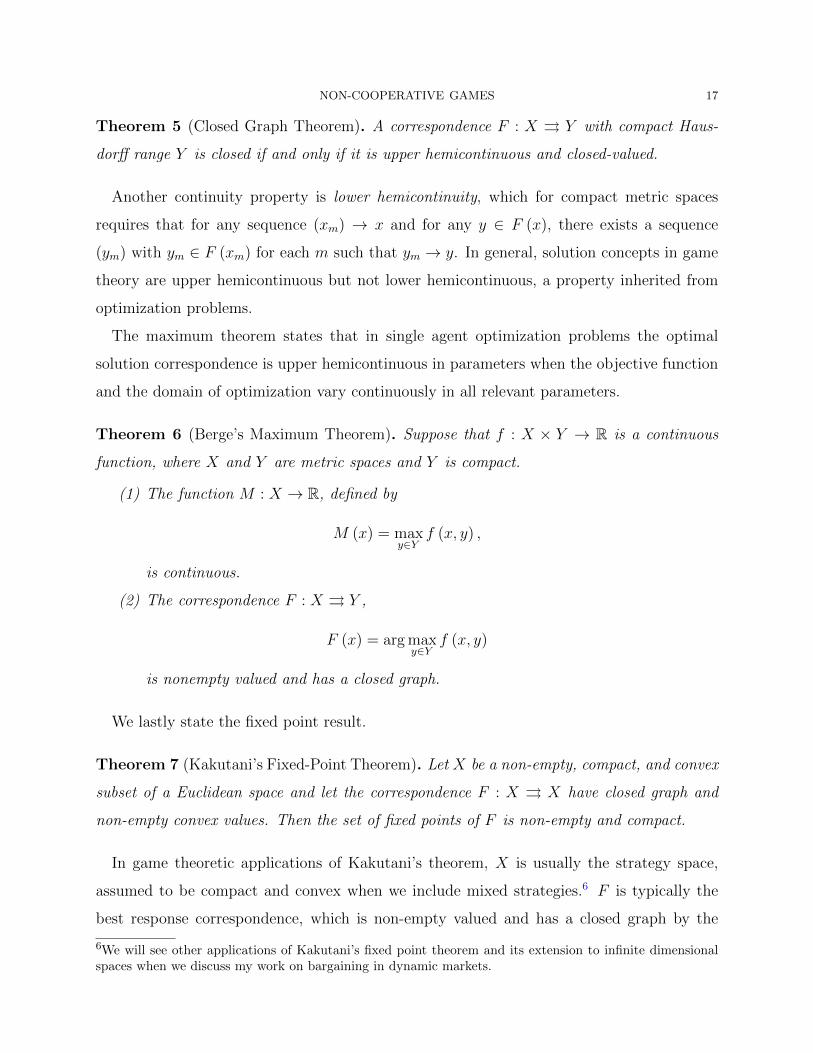
Theorem 5 (Closed Graph Theorem). A correspondence F : X ⇒ Y with compact Haus-
dorff range Y is closed if and only if it is upper hemicontinuous and closed-valued.
Another continuity property is lower hemicontinuity, which for compact metric spaces
requires that for any sequence (xm) → x and for any y ∈ F (x), there exists a sequence
(ym) with ym ∈ F (xm) for each m such that ym → y. In general, solution concepts in game
theory are upper hemicontinuous but not lower hemicontinuous, a property inherited from
optimization problems.
The maximum theorem states that in single agent optimization problems the optimal
solution correspondence is upper hemicontinuous in parameters when the objective function
and the domain of optimization vary continuously in all relevant parameters.
Theorem 6 (Berge’s Maximum Theorem). Suppose that f : X × Y → R is a continuous
function, where X and Y are metric spaces and Y is compact.
(1) The function M : X → R, defined by
M (x) = max f (x, y) ,y∈Y
is continuous.
(2) The correspondence F : X ⇒ Y ,
F (x) = arg max f (x, y)y∈Y
is nonempty valued and has a closed graph.
We lastly state the fixed point result.
Theorem 7 (Kakutani’s Fixed-Point Theorem). Let X be a non-empty, compact, and convex
subset of a Euclidean space and let the correspondence F : X ⇒ X have closed graph and
non-empty convex values. Then the set of fixed points of F is non-empty and compact.
In game theoretic applications of Kakutani’s theorem, X is usually the strategy space,
assumed to be compact and convex when we include mixed strategies.6 F is typically the
best response correspondence, which is non-empty valued and has a closed graph by the
6We will see other applications of Kakutani’s fixed point theorem and its extension to infinite dimensionalspaces when we discuss my work on bargaining in dynamic markets.
18 MIHAI MANEA
Maximum Theorem. In that case, we can ensure that F is convex-valued by assuming that
the payoff functions are quasi-concave.
Recall that a function f : X → R is quasi-concave when X is a convex subset of a real
vector space if
f(tx+ (1− t)y) ≥ min(f(x), f(y)),∀t ∈ [0, 1], x, y ∈ X.
In particular, quasi-concavity implies convex upper contour sets and convex arg max.
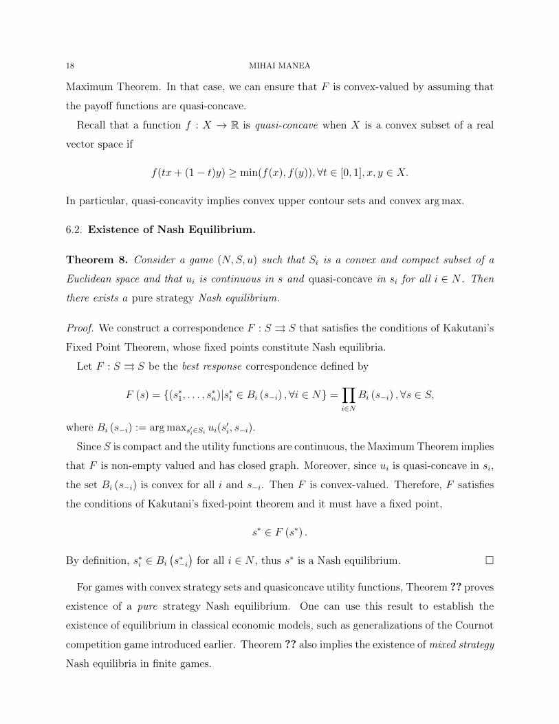
6.2. Existence of Nash Equilibrium.
Theorem 8. Consider a game (N,S, u) such that Si is a convex and compact subset of a
Euclidean space and that ui is continuous in s and quasi-concave in si for all i ∈ N . Then
there exists a pure strategy Nash equilibrium.
Proof. We construct a correspondence F : S ⇒ S that satisfies the conditions of Kakutani’s
Fixed Point Theorem, whose fixed points constitute Nash equilibria.
Let F : S ⇒ S be the best response correspondence defined by
F (s) = (s∗1, . . . , s∗n)|s∗i ∈ Bi (s−i) ,∀i ∈ N =∏
Bi (s ) , s S,−ii
∀ ∈∈N
where Bi (s i) := arg max− s′∈Siui(s
′i, s−i).i
Since S is compact and the utility functions are continuous, the Maximum Theorem implies
that F is non-empty valued and has closed graph. Moreover, since ui is quasi-concave in si,
the set Bi (s−i) is convex for all i and s−i. Then F is convex-valued. Therefore, F satisfies
the conditions of Kakutani’s fixed-point theorem and it must have a fixed point,
s∗ ∈ F (s∗) .
By definition, s∗i ∈ Bi
(s∗ i)
for all i ∈ N , thus s∗ is a Nash equilibrium. −
For games with convex strategy sets and quasiconcave utility functions, Theorem ?? proves
existence of a pure strategy Nash equilibrium. One can use this result to establish the
existence of equilibrium in classical economic models, such as generalizations of the Cournot
competition game introduced earlier. Theorem ?? also implies the existence of mixed strategy
Nash equilibria in finite games.
NON-COOPERATIVE GAMES 19
Corollary 3. Every finite game has a mixed strategy Nash equilibrium.
Proof. Since S is finite, each ∆ (Si) is isomorphic to a simplex in a Euclidean space, which is
convex and compact. Player i’s expected utility ui (σ) =∑
s ui (s)σ1 (s1) · · ·σn (sn) from a
mixed strategy profile σ is continuous in σ and linear—hence also quasi-concave—in σi. Then
the game (N,∆ (S1) , . . . ,∆ (Sn) , u) satisfies the assumptions of Theorem ??. Therefore, it
admits a Nash equilibrium σ∗ ∈ ∆ (S1)× · · · ×∆ (Sn), which can be interpreted as a mixed
Nash equilibrium in the original game.
6.3. Upperhemicontinuity of Nash Equilibrium. The Maximum Theorem establishes
that the best-response correspondence in optimization problems is upper hemicontinuous in
parameters when the payoffs are continuous and the domain is compact. Hence the limits of
optimal solutions is a solution to the optimization problem in the limit. One can then find
a solution by considering approximate problems and taking the limit. There can be other
solutions in the limit, so the best response correspondence is not lower hemicontinuous in
general. Nash equilibrium (like many other solution concepts) inherits these properties of
the best response correspondence.
Consider a compact metric space X of some payoff-relevant parameters. Fix a set N of
players and set S of strategy profiles, where S is again a compact metric space (or a finite
set). The payoff function ui : S × X → R of every i ∈ N is assumed to be continuous
in both strategies and parameters. Write NE (x) and PNE (x) for the sets of all Nash
equilibria and all pure Nash equilibria, respectively, of game (N,S, u (·, x)) in which it is
common knowledge that the parameter value is x. Endow the space of mixed strategies with
the weak topology.
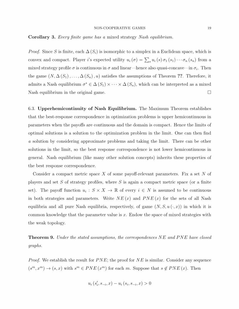
Theorem 9. Under the stated assumptions, the correspondences NE and PNE have closed
graphs.
Proof. We establish the result for PNE; the proof for NE is similar. Consider any sequence
(sm, xm)→ (s, x) with sm ∈ PNE (xm) for each m. Suppose that s 6∈ PNE (x). Then
ui (s′i, s i, x)− − ui (si, s−i, x) > 0
20 MIHAI MANEA
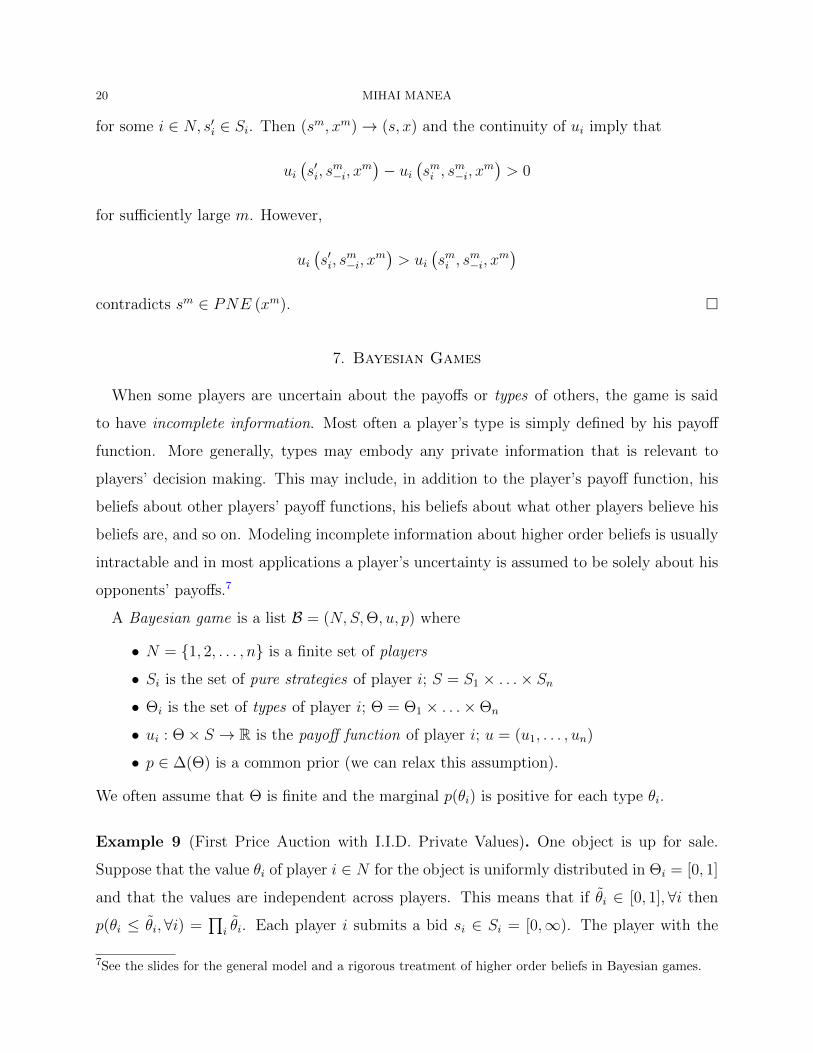
for some i ∈ N, s′i ∈ Si. Then (sm, xm)→ (s, x) and the continuity of ui imply that
ui s′i, s
mi, x
m >− − ui sm, sm mi 0−i, x
for sufficiently large m. Howev
(er,
) ( )
ui(s′i, s
mi, x
m)> ui
(smi , s
mi, x
m− −
contradicts sm
)∈ PNE (xm).
7. Bayesian Games
When some players are uncertain about the payoffs or types of others, the game is said
to have incomplete information. Most often a player’s type is simply defined by his payoff
function. More generally, types may embody any private information that is relevant to
players’ decision making. This may include, in addition to the player’s payoff function, his
beliefs about other players’ payoff functions, his beliefs about what other players believe his
beliefs are, and so on. Modeling incomplete information about higher order beliefs is usually
intractable and in most applications a player’s uncertainty is assumed to be solely about his
opponents’ payoffs.7
A Bayesian game is a list B = (N,S,Θ, u, p) where
• N = 1, 2, . . . , n is a finite set of players
• Si is the set of pure strategies of player i; S = S1 × . . .× Sn• Θi is the set of types of player i; Θ = Θ1 × . . .×Θn
• ui : Θ× S → R is the payoff function of player i; u = (u1, . . . , un)
• p ∈ ∆(Θ) is a common prior (we can relax this assumption).
We often assume that Θ is finite and the marginal p(θi) is positive for each type θi.
Example 9 (First Price Auction with I.I.D. Private Values). One object is up for sale.
Suppose that the value θi of player i ∈ N for the object is uniformly distributed in Θi = [0, 1]
˜and that the values are independent across players. This means that if θi ∈ [0, 1],∀i then
p(θi ≤ θi,∀ ˜i) =∏
i θi. Each player i submits a bid si ∈ Si = [0,∞). The player with the
7See the slides for the general model and a rigorous treatment of higher order beliefs in Bayesian games.
NON-COOPERATIVE GAMES 21
highest bid wins the object and pays his bid. Ties are broken randomly. Hence the payoffs
are given by
i
ui(θ, s) =
θi−s
if s s| ∈ | | i ≥ j,j N si=sj∀j ∈ N
0 otherwise.
Example 10 (An exchange game). Each player i = 1, 2 receives a ticket on which there
is a number in some finite set Θi ⊂ [0, 1]. The number on a player’s ticket represents
the size of a prize he may receive. The two prizes are independently distributed, with the
value on i’s ticket distributed according to Fi. Each player is asked independently and
simultaneously whether he wants to exchange his prize for the other player’s prize, hence
Si = agree, disagree. If both players agree then the prizes are exchanged; otherwise each
player receives his own prize. Thus thepayoff of player i isθ3 i if s =− 1 s2 = agreeui(θ, s) =
θi otherwise.
In the ex ante representationG(B) of
the Bayesian game B player i has strategies (si(θi))θi∈Θi
∈
SΘii —that is, his strategies are functions from types to strategies in B—and utility function
Ui given by
Ui((si(θi))θi∈Θi,i N) = Ep(ui(θ, s1(θ )∈ 1 , . . . , sn(θn))).
The interim representation IG(B) of the Bayesian game B has player set ∪iΘi. The
strategy space of each player θi is Si. A strategy profile (sθi)i∈N,θi yields∈Θiutility
Uθi((sθi)i∈N,θi∈Θi) = Ep(ui(θ, sθ1 , . . . , sθn)|θi)
for player θi. For the conditional expectation to be well-defined we need p(θi) > 0.
Definition 13. A Bayesian Nash equilibrium of B is a Nash equilibrium of IG(B).
Proposition 1. Every Bayesian Nash equilibrium of B is a Nash equilibrium of G(B). If
p(θ 8i) > 0 for all θi ∈ Θi, i ∈ N , the converse also holds.
Theorem 10. Suppose that
• N and Θ are finite
8Strategies are mapped between the two games by si(θi)→ sθi .
22 MIHAI MANEA
• each Si is a compact and convex subset of a Euclidean space
• each ui is continuous in s and concave in si.
Then B has a pure strategy Bayesian Nash equilibrium.
Proof. We have to show that IG(B) has a pure Nash equilibrium. The latter follows from
Theorem ??. We use the concavity of ui in si to show that the corresponding Uθi is quasi-
concave in sθi . Quasi-concavity of ui in si does not typically imply quasi-concavity of Uθi in
s 9θi because Uθi is an integral of ui over variables other than sθi .
Example 11 (Study groups). Two students work on a joint project. Each student i can
either exert effort (ei = 1) or shirk (ei = 0). The cost of effort is a fixed (and commonly
known) c < 1 for all students. The project is a success if at least one student puts in effort,
but both fail otherwise. However, students vary in how much they care about the fate of the
project. Concretely, each student i has a type θi ∼ U [0, 1]; the types of both students are
independently distributed and privately known. The payoff from success is θ2i , so a student
gets θ2i − c from working, θ2
i from shirking if j works, and 0 if both shirk.
This game has a unique Bayesian Nash equilibrium. In equilibrium, both players use a1
threshold strategy: i works if θi ≥ θ∗ = c 3 , and shirks otherwise. For a proof, note that
working is rational for i iff
θ2i − c ≥ θ2
i pj ⇐⇒ (1− pj)θ2i ≥ c,
where pj is i’s belief about the probability that j will work. (Crucially, since types are
independent, p does not
with threshold θi∗ =
√ depend on θi). This implies that i must play a threshold strategy,
c1−pj . Since the same is true of player j, we have pj = 1 − θ∗j , so
θ∗i =√
c . This is true for i = 1, j = 2 and vice-versa, which implies the result.θj∗
Consider a family of Bayesian games Bx parameterized by x ∈ X, with X compact, such
that the payoff functions are continuous in x. If S,Θ are finite, then the set of Bayesian
Nash equilibria of Bx is upper-hemicontinuous with respect to x. Indeed, BNE(Bx) =
NE(IG(Bx)). Furthermore, we have upper-hemicontinuity with respect to beliefs.
Theorem 11. Suppose that N,S,Θ are finite. Let P ⊂ ∆(Θ) be such that for every p ∈ P
p(θi) > 0,∀θi ∈ Θ pi, i ∈ N . Then BNE(B ) is upper-hemicontinuous in p over P .
9Sums of quasi-concave functions are not necessarily quasi-concave.
NON-COOPERATIVE GAMES 23
Proof. Since BNE(Bp) = NE(IG(Bp)), it is sufficient to note that
Ui((si(θi))θi∈Θi,i∈N) = Ep(ui(θ, s1(θ1), . . . , sn(θn)))
(as defined for G(Bp)) is continuous in p.
8. Auctions
In class we covered (see handouts)
(1) the characterization of equilibria in first and second price auctions (pp. 14-20 in
“Auction Theory” by Vijay Krishna)
(2) the revenue equivalence theorem and optimal auctions (pp. 61-73 in “Auction The-
ory”)
(3) all-pay and third-price auctions (pp. 31-34 in “Auction Theory”)
(4) first-price auction with two asymmetric bidders (pp. 49-53 in “Auction Theory”)
(5) bilateral trade and the inefficiency theorem of Myerson and Satterthwaite (1983).
9. Extensive Form Games
An extensive form game consists of
• a finite set of players N = 1, 2, . . . , n; nature is denoted as “player 0”
• the order of moves specified by a tree
• each player’s payoffs at the terminal nodes in the tree
• information partition
• the set of actions available at every information set and a description of how actions
lead to progress in the tree
• moves by nature.
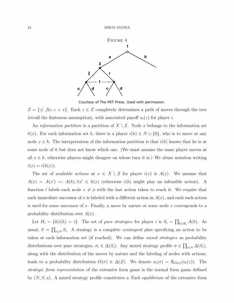
Go over the extensive form Figure ?? (FT, p. 86).
The tree is described by a binary relationship (X,>), where x > y is interpreted as “node
x precedes node y.” We assume that X is finite, there is an initial node φ ∈ X (φ > x
for all x 6= φ), > is transitive (x > y, y > z ⇒ x > z) and asymmetric (x > y ⇒ y 6> x).
Hence the tree has no cycles. We also require that each node x 6= φ has exactly one
immediate predecessor, i.e., ∃x′ > x such that x′′ > x, x′′ 6= x′ implies x′′ > x′. A node is
terminal if it does not precede any other node; this means that the set of terminal nodes is
24 MIHAI MANEA
Figure 4
Courtesy of The MIT Press. Used with permission.
Z = z| 6 ∃x, z > x. Each z ∈ Z completely determines a path of moves through the tree
(recall the finiteness assumption), with associated payoff ui(z) for player i.
An information partition is a partition of X \ Z. Node x belongs to the information set
h(x). For each information set h, there is a player i(h) ∈ N ∪ 0, who is to move at any
node x ∈ h. The interpretation of the information partition is that i(h) knows that he is at
some node of h but does not know which one. (We must assume the same player moves at
all x ∈ h, otherwise players might disagree on whose turn it is.) We abuse notation writing
i(x) = i(h(x)).
The set of available actions at x ∈ X \ Z for player i(x) is A(x). We assume that
A(x) = A(x′) =: A(h),∀x′ ∈ h(x) (otherwise i(h) might play an infeasible action). A
function l labels each node x 6= φ with the last action taken to reach it. We require that
each immediate successor of x is labeled with a different action in A(x), and each such action
is used for some successor of x. Finally, a move by nature at some node x corresponds to a
probability distribution over A(x).
Let Hi = h|i(h) = i. The set of pure strategies for player i is Si = h∈H A(h). Asi
usual, S =∏
i N Si. A strategy is a complete contingent plan specifying
∏an action to be∈
taken at each information set (if reached). We can define mixed strategies as probability
distributions over pure strategies, σi ∈ ∆(Si). Any mixed strategy profile σ ∈
along with the distribution of the moves by nature and the labeling of nodes with
∏i N ∆(Si),∈
actions,
leads to a probability distribution O(σ) ∈ ∆(Z). We denote ui(σ) = EO(σ)(ui(z)). The
strategic form representation of the extensive form game is the normal form game defined
by (N,S, u). A mixed strategy profile constitutes a Nash equilibrium of the extensive form
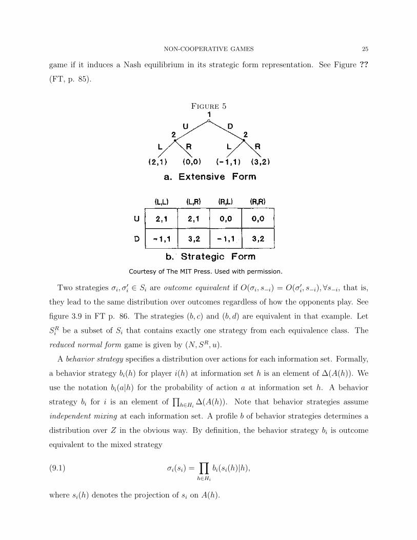
NON-COOPERATIVE GAMES 25
game if it induces a Nash equilibrium in its strategic form representation. See Figure ??
(FT, p. 85).
Figure 5
Two strategies σi, σi′ ∈ Si are outcome equivalent if O(σi, s i) = O(σi
′, s i),∀s i, that is,− − −
they lead to the same distribution over outcomes regardless of how the opponents play. See
figure 3.9 in FT p. 86. The strategies (b, c) and (b, d) are equivalent in that example. Let
SRi be a subset of Si that contains exactly one strategy from each equivalence class. The
reduced normal form game is given by (N,SR, u).
A behavior strategy specifies a distribution over actions for each information set. Formally,
a behavior strategy bi(h) for player i(h) at information set h is an element of ∆(A(h)). We
use the notation bi(a|h) for the probability of action a at information set h. A behavior
strategy bi for i is an element of∏
h H ∆(A(h)). Note that behavior strategies assume∈ i
independent mixing at each information set. A profile b of behavior strategies determines a
distribution over Z in the obvious way. By definition, the behavior strategy bi is outcome
equivalent to the mixed strategy
(9.1) σi(si) =∏
bi(si(h)|h),h∈Hi
where si(h) denotes the projection of si on A(h).
Courtesy of The MIT Press. Used with permission.

26 MIHAI MANEA
To guarantee that every mixed strategy is equivalent to a behavior strategy (reinterpreted
as a mixed strategy as above) we need to impose the additional requirement of perfect recall.
Basically, perfect recall means that no player ever forgets any information he once had and
all players know the actions they have chosen previously. Formally, perfect recall stipulates
that if x′′ ∈ h(x′), x is a predecessor of x′ and the same player i moves at both x and x′ (and
thus at x′′) then there is a node x in the same information set as x (possibly x itself) such
that x is a predecessor of x′′ and the action taken at x along the path to x′ is the same as the
action taken at x along the path to x′′. Intuitively, the nodes x′ and x′′ are distinguished by
information i does not have, so he cannot have had it at h(x); x′ and x′′ must be consistent
with the same action at h(x) since i must remember his action there. Stated differently,
every node in h ∈ Hi must be reached via the same sequence of i’s actions.
Discuss the absent-minded driver’s paradox of Piccione and Rubinstein (1997).
Let Ri(h) be the set of pure strategies for player i that do not preclude reaching the
information set h ∈ Hi, i.e., Ri(h) = si|h is on the path of (si, s−i) for some s−i. If the
game has perfect recall, a mixed strategy σi is equivalent to a behavior strategy bi defined
by
σ (s )(9.2) bi(a|
∑s (
hsi∈Ri(h)| i h)=a i i
) =
when
∑si∈Ri(h) σi(si)
the denominator is positive, and letting bi(h) be any distribution when the above
denominator is zero.
For some intuition, let h1, . . . , hk be player i’s information sets preceding h in the tree. In
a game of perfect recall, reaching any node in h requires i to take the same action ak at each
hk. Then Ri(h) is simply the set of pure strategies si with si(hk) = ak for all k. Reaching
any node x in h requires player i to choose a1, . . . , ak and other players to also take specific
actions. Conditional on getting to x, the distribution of continuation play at x is given by
the relative probabilities of the actions available at h under the restriction of σi to the set
of pure strategies si|si(hk) = ak,∀k = 1, k compatible with reaching h,
bi(a|h) =
∑si|si(hk)=ak,∀k=1,k & si(h)=a σi(si)∑
si|si(hk)=ak,∀k=
.¯ σ (,k i si)1
Many different mixed strategies can generate the same behavior strategy. Consider the
example from Figure ?? (FT, p. 88). Player 2 has four pure strategies, s2 = (A,C), s′2 =
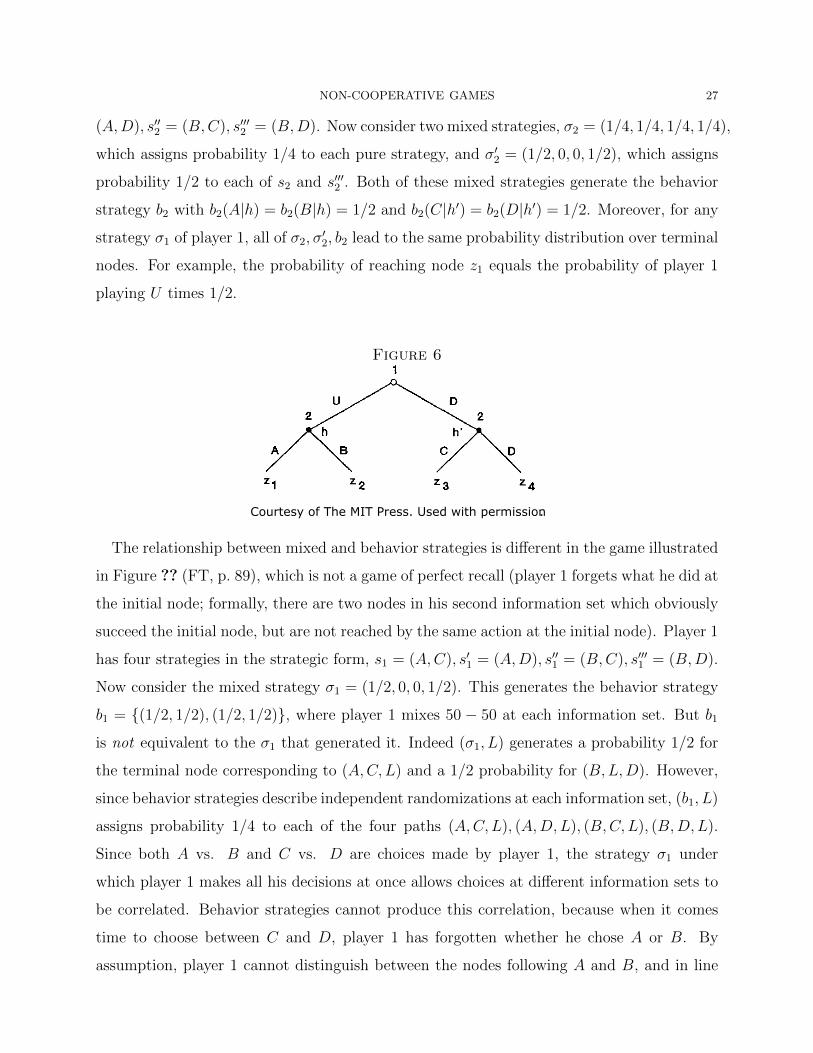
NON-COOPERATIVE GAMES 27
(A,D), s′′2 = (B,C), s′′′2 = (B,D). Now consider two mixed strategies, σ2 = (1/4, 1/4, 1/4, 1/4),
which assigns probability 1/4 to each pure strategy, and σ2′ = (1/2, 0, 0, 1/2), which assigns
probability 1/2 to each of s2 and s′′′2 . Both of these mixed strategies generate the behavior
strategy b2 with b2(A|h) = b2(B|h) = 1/2 and b2(C|h′) = b2(D|h′) = 1/2. Moreover, for any
strategy σ1 of player 1, all of σ2, σ2′ , b2 lead to the same probability distribution over terminal
nodes. For example, the probability of reaching node z1 equals the probability of player 1
playing U times 1/2.
Figure 6
Courtesy of The MIT Press. Used with permission.
The relationship between mixed and behavior strategies is different in the game illustrated
in Figure ?? (FT, p. 89), which is not a game of perfect recall (player 1 forgets what he did at
the initial node; formally, there are two nodes in his second information set which obviously
succeed the initial node, but are not reached by the same action at the initial node). Player 1
has four strategies in the strategic form, s1 = (A,C), s′1 = (A,D), s′′1 = (B,C), s′′′1 = (B,D).
Now consider the mixed strategy σ1 = (1/2, 0, 0, 1/2). This generates the behavior strategy
b1 = (1/2, 1/2), (1/2, 1/2), where player 1 mixes 50 − 50 at each information set. But b1
is not equivalent to the σ1 that generated it. Indeed (σ1, L) generates a probability 1/2 for
the terminal node corresponding to (A,C, L) and a 1/2 probability for (B,L,D). However,
since behavior strategies describe independent randomizations at each information set, (b1, L)
assigns probability 1/4 to each of the four paths (A,C, L), (A,D,L), (B,C, L), (B,D,L).
Since both A vs. B and C vs. D are choices made by player 1, the strategy σ1 under
which player 1 makes all his decisions at once allows choices at different information sets to
be correlated. Behavior strategies cannot produce this correlation, because when it comes
time to choose between C and D, player 1 has forgotten whether he chose A or B. By
assumption, player 1 cannot distinguish between the nodes following A and B, and in line
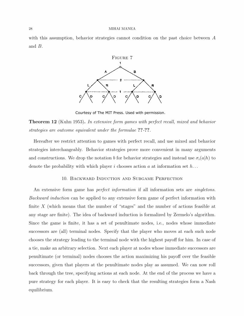
28 MIHAI MANEA
with this assumption, behavior strategies cannot condition on the past choice between A
and B.
Figure 7
Courtesy of The MIT Press. Used with permission.
Theorem 12 (Kuhn 1953). In extensive form games with perfect recall, mixed and behavior
strategies are outcome equivalent under the formulae ??-??.
Hereafter we restrict attention to games with perfect recall, and use mixed and behavior
strategies interchangeably. Behavior strategies prove more convenient in many arguments
and constructions. We drop the notation b for behavior strategies and instead use σi(a|h) to
denote the probability with which player i chooses action a at information set h. . .
10. Backward Induction and Subgame Perfection
An extensive form game has perfect information if all information sets are singletons.
Backward induction can be applied to any extensive form game of perfect information with
finite X (which means that the number of “stages” and the number of actions feasible at
any stage are finite). The idea of backward induction is formalized by Zermelo’s algorithm.
Since the game is finite, it has a set of penultimate nodes, i.e., nodes whose immediate
successors are (all) terminal nodes. Specify that the player who moves at each such node
chooses the strategy leading to the terminal node with the highest payoff for him. In case of
a tie, make an arbitrary selection. Next each player at nodes whose immediate successors are
penultimate (or terminal) nodes chooses the action maximizing his payoff over the feasible
successors, given that players at the penultimate nodes play as assumed. We can now roll
back through the tree, specifying actions at each node. At the end of the process we have a
pure strategy for each player. It is easy to check that the resulting strategies form a Nash
equilibrium.
NON-COOPERATIVE GAMES 29
Theorem 13 (Zermelo 1913; Kuhn 1953). A finite game of perfect information has a pure-
strategy Nash equilibrium.
Moreover, the backward induction solution has the nice property that, if play starts at
any intermediate node, each player’s actions are again optimal if the play of the opponents is
held fixed, which we call subgame perfection. This rules out non-credible threats in response
to deviations from the prescribed play. More generally, subgame perfection extends the logic
of backward induction to games with imperfect information. The idea is to replace the
“smallest” subgame with one of its Nash equilibria and iterate this procedure on the reduced
tree. In stages where the “smallest” subgame has multiple Nash equilibria, the procedure
implicitly assumes that all players believe the same equilibrium will be played. To define
subgame perfection formally we first need the definition of a subgame. Informally, a subgame
is a portion of a game that can be analyzed as a game in its own right.
Definition 14. A subgame G of an extensive form game T consists of a single node x and
all its successors in T , with the property that if x′ ∈ G and x′′ ∈ h(x′) then x′′ ∈ G. The
information sets, actions and payoffs of the subgame are inherited from the original game.
That is, two nodes are in the same information set in G if and only if they are in the same
information set in T , and the payoff function on the subgame is just the restriction of the
original payoff function to the terminal nodes of G (and likewise for the action sets and
action labels).
The requirements that all the successors of x be in the subgame and that the subgame
does not “chop up” any information set ensure that the subgame corresponds to a situation
that could arise in the original game. At the top of Figure ?? (FT, p. 95), the game on
the right is not a subgame of the game on the left, because on the right player 2 knows that
player 1 has not played L, which he did not know in the original game.
Together, the requirements that the subgame begin with a single node x and respect
information sets imply that in the original game x must be a singleton information set,
i.e. h(x) = x. This ensures that the distribution over paths of play and payoffs in the
subgame, conditional on the subgame being reached, are well defined. In the bottom of
Figure ??, the “game” on the right has the problem that player 2’s optimal choice may
depend on the relative probabilities of nodes x and x′, but the specification of the game does
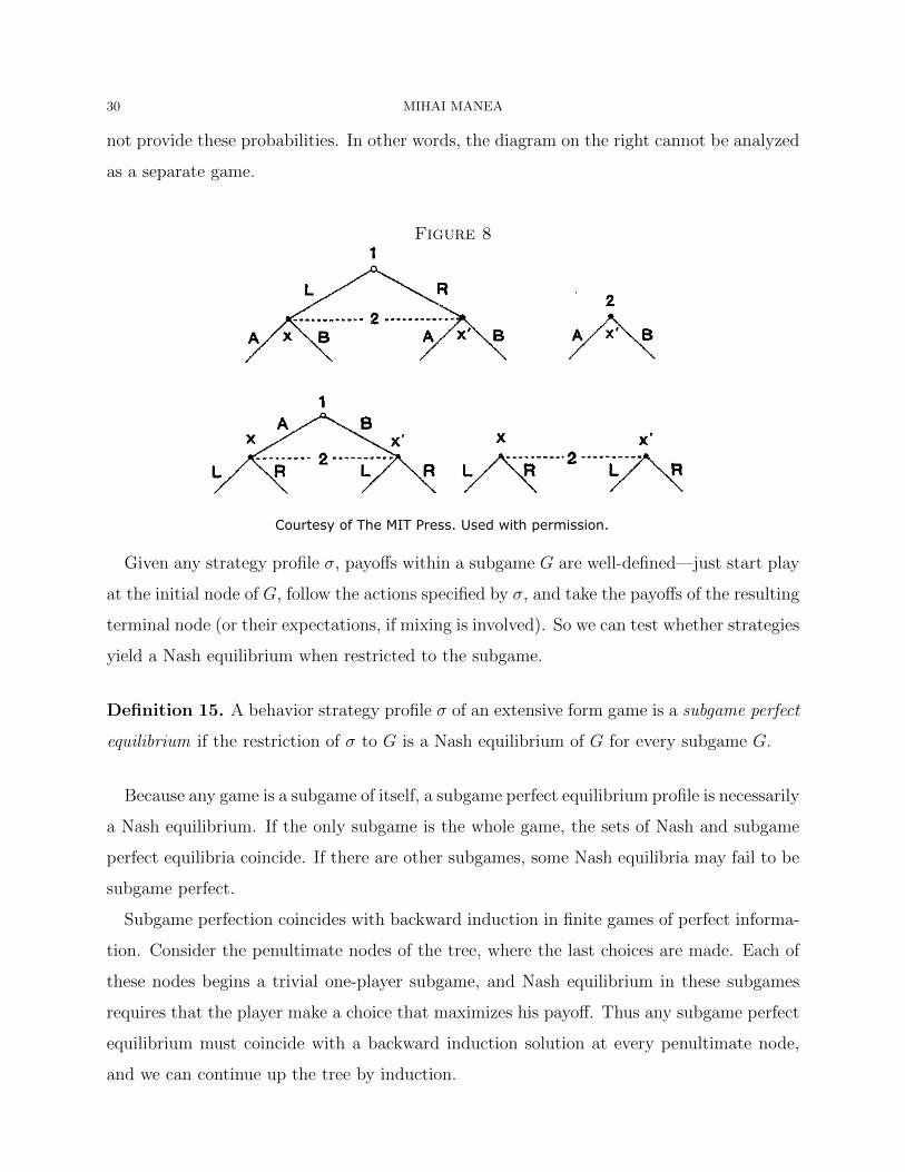
30 MIHAI MANEA
not provide these probabilities. In other words, the diagram on the right cannot be analyzed
as a separate game.
Figure 8
Courtesy of The MIT Press. Used with permission.
Given any strategy profile σ, payoffs within a subgame G are well-defined—just start play
at the initial node of G, follow the actions specified by σ, and take the payoffs of the resulting
terminal node (or their expectations, if mixing is involved). So we can test whether strategies
yield a Nash equilibrium when restricted to the subgame.
Definition 15. A behavior strategy profile σ of an extensive form game is a subgame perfect
equilibrium if the restriction of σ to G is a Nash equilibrium of G for every subgame G.
Because any game is a subgame of itself, a subgame perfect equilibrium profile is necessarily
a Nash equilibrium. If the only subgame is the whole game, the sets of Nash and subgame
perfect equilibria coincide. If there are other subgames, some Nash equilibria may fail to be
subgame perfect.
Subgame perfection coincides with backward induction in finite games of perfect informa-
tion. Consider the penultimate nodes of the tree, where the last choices are made. Each of
these nodes begins a trivial one-player subgame, and Nash equilibrium in these subgames
requires that the player make a choice that maximizes his payoff. Thus any subgame perfect
equilibrium must coincide with a backward induction solution at every penultimate node,
and we can continue up the tree by induction.
NON-COOPERATIVE GAMES 31
11. Important Examples of Extensive Form Games
11.1. Repeated games with perfect monitoring.
• time t = 0, 1, 2, . . . (usually infinite)
• stage game is a normal-form game G
• G is played every period t
• players observe the realized actions at the end of each period
• payoffs are the sum of discounted payoffs in the stage game.
Repeated games are a widely studied class of dynamic games. A lot of recent research deals
with the case of imperfect monitoring.
11.2. Multi-stage games with observable actions.
• stages t = 0, 1, 2, . . .
• at stage t, after having observed a “non-terminal” history of play h = (a0, . . . , at−1),
each player i simultaneously chooses an action ati ∈ Ai(h)
• payoffs given by u(h) for each terminal history h.
Often it is natural to identify the “stages” of the game with time periods, but this is not
always the case. A game of perfect information can be viewed as a multi-stage game in which
every stage corresponds to some node. At every stage all but one player (the one moving
at the node corresponding to that stage) have singleton action sets (“do nothing”; we can
refer to these players as “inactive”). Repeated versions of perfect information extensive form
games also lead to multi-stage games. Another important example is the Rubinstein (1982)
alternating bargaining game, which we discuss later.
12. Single (or One-Shot) Deviation Principle
Consider a multi-stage game with observed actions. We show that in order to verify that a
strategy profile σ constitutes a subgame perfect equilibrium, it suffices to check whether there
are any histories ht where some player i can gain by deviating from the action prescribed by
σi at ht and conforming to σi elsewhere. (The notation ht denotes a history as of stage t.)
If σ is a strategy profile and ht a history, write ui(σ|ht) for the (expected) payoff to player
i that results if play starts at ht and continues according to σ in each stage.
32 MIHAI MANEA
Definition 16. A (behavior) strategy σi is unimprovable given σ−i if ui(σi, σ−i|ht) ≥
ui(σi′, σ i|ht) for every h and− t σi
′ with σi′(h′t ) = σ′ i(h
′t ) for all h′
′t′ 6= ht.
Hence a strategy σi is unimprovable if after every history, no strategy that differs from
it only at that history can increase i’s expected payoff. Obviously, if σ is a subgame per-
fect equilibrium then σi is unimprovable given σ i. To establish the converse, we need an−
additional condition.
Definition 17. A game is continuous at infinity if for each player i the utility function ui
satisfies
lim sup |ui(h)t→∞ ˜ ˜(h,h) ht=ht
− ˜ui(h)| = 0. |
Continuity at infinity requires that events in the distant future are relatively unimportant.
It is satisfied if the overall payoffs are a discounted sum of per-period payoffs and the stage
payoffs are uniformly bounded. It also holds in the (degenerate) case of finite-stage games.
There exist versions for games with unobserved actions as well.
Theorem 14. Consider a (finite or infinite horizon) multi-stage game with observed ac-
tions10 that is continuous at infinity. If σi is unimprovable given σ then−i for all i ∈ N , σ
constitutes an SPE.
Proof. Suppose that σi is unimprovable given σ i, but σ is− i not a best response to σ−i
following some history h 1t. Let σi be a strictly better response and define
(12.1) ε = ui(σ1i , σ−i|ht)− ui(σi, σ−i|ht) > 0.
Since the game is continuous at infinity, there exists t′ > t and σ2i such that σ2
i is identical
to σ1i at all information sets up to (and including) stage t′, σ2
i coincides with σi across all
longer histories and
(12.2) |ui(σ2i , σ−i|ht)− u 1
i(σi , σ−i|ht)| < ε/2.
In particular, ?? and ?? imply that
ui(σ2i , σ i|h )− t > ui(σi, σ−i|ht).
10We allow for the possibility that the action set be infinite at some stages.
NON-COOPERATIVE GAMES 33
Denote by σ3i the strategy obtained from σ2
i by replacing the stage t′ actions following
any history ht′ with the corresponding actions under σi. Conditional on any history ht′ , the
strategies σi and σ3i coincide, hence
(12.3) u 3i(σi , σ−i|ht′) = ui(σi, σ−i|ht′).
As σi is unimprovable given σ−i, and conditional on ht′ the subsequent play in strategies σi
and σ2i differs only at stage t′, we must have
(12.4) ui(σi, σ2
−i|ht′) ≥ ui(σi , σ h ).−i| t′
Then ?? and ?? lead to
ui(σ3i , σ i|ht′) ≥ ui(σ
2i , σ h− −i| t′)
for all histories h 2 3t′ (consistent with ht). Since σi and σi coincide before reaching stage t′,
we obtain
ui(σ3i , σ i|ht) ≥ ui(σ
2i , σ h− −i| t).
Similarly, we can construct σ4 ′ ′
i , . . . , σt −t+3i . The final strategy σti
−t+3 is identical to σi
conditional on ht and
ui(σt′ t+3 3 2
i, σ ) = u−i|ht i(σi− , σ−i|ht) ≥ . . . ≥ ui(σi , σ−i|ht) ≥ ui(σi , σ−i|ht) > ui(σi, σ−i|ht),
a contradiction.
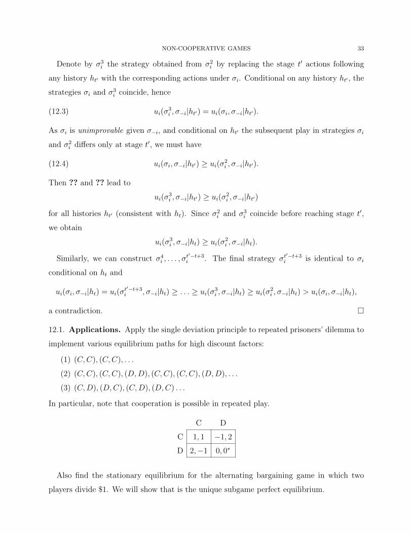
12.1. Applications. Apply the single deviation principle to repeated prisoners’ dilemma to
implement various equilibrium paths for high discount factors:
(1) (C,C), (C,C), . . .
(2) (C,C), (C,C), (D,D), (C,C), (C,C), (D,D), . . .
(3) (C,D), (D,C), (C,D), (D,C) . . .
In particular, note that cooperation is possible in repeated play.
C D
C 1, 1 −1, 2
D 2,−1 0, 0∗
Also find the stationary equilibrium for the alternating bargaining game in which two
players divide $1. We will show that is the unique subgame perfect equilibrium.

34 MIHAI MANEA
13. Iterated Conditional Dominance
Definition 18. In a multi-stage game with observable actions, an action ai is conditionally
dominated at stage t given history ht if, in the subgame starting at ht, every strategy for
player i that assigns positive probability to ai is strictly dominated.
Proposition 2. In any multi-stage game with observable actions, every subgame perfect
equilibrium survives iterated elimination of conditionally dominated strategies.
14. Bargaining with Alternating Offers
One important example of a multi-stage game with observed actions is the following bar-
gaining game, analyzed by Rubinstein (1982).
The set of players is N = 1, 2. For i = 1, 2 we write j = 3− i. The set of feasible utility
pairs is
U = (u1, u2) ∈ [0,∞)2|u2 ≤ g2(u1),
where g2 is some strictly decreasing, concave (and hence continuous) function with g2(0) >
0.11
Time is discrete and infinite, t = 0, 1, . . . Each player i discounts payoffs by δi, so receiving
u ti at time t is worth δiui.
At every time t = 0, 1, . . ., player i(t) proposes an alternative u = (u1, u2) ∈ U to player
j(t) = 3 − i(t); the bargaining protocol specifies that i(t) = 1 for t even and i(t) = 2 for
t odd. If j(t) accepts the offer, then the game ends yielding a payoff vector (δt1u1, δt2u2).
Otherwise, the game proceeds to period t + 1. If agreement is never reached, each player
receives a 0 payoff.
It is useful to define the function g1 = g−12 . Notice that the graph of g2 (and g−1
1 ) coincides
with the Pareto-frontier of U .
11The set of feasible utility outcomes U can be generated from a set of contracts or decisions X in a naturalway. Define U = (v1 (x) , v2 (x)) |x ∈ X for a pair of utility functions v1 and v2 over X. With additionalassumptions on X, v1, v2 we can ensure that the resulting U is compact and convex.

NON-COOPERATIVE GAMES 35
14.1. Stationary subgame perfect equilibrium. Let (m1,m2) be the unique solution to
the following system of equations
m1 = δ1g1 (m2)
m2 = δ2g2 (m1) .
Note that (m1,m2) is the intersection of the graphs of the functions δ2g2 and (δ1g1)−1.
We are going to argue that the following “stationary” strategies constitute a subgame
perfect equilibrium, and that any other subgame perfect equilibrium leads to the same out-
come. In any period where player i has to make an offer to j, he offers u with uj = mj and j
accepts only offers u with uj ≥ mj. We can use the single-deviation principle to check that
the constructed strategies form a subgame perfect equilibrium.
14.2. Equilibrium uniqueness. We can use iterated conditional dominance to rule out
many actions and then prove that the stationary equilibrium is essentially the unique sub-
game perfect equilibrium.
Theorem 15. The subgame perfect equilibrium is unique, except for the decision to accept
or reject Pareto-inefficient offers.
Proof. Player i cannot obtain a period t expected payoff greater than
M0i = δi maxui = δigi(0)
u∈U
following a disagreement at date t. Hence rejecting an offer u with ui > M0i is conditionally
dominated by accepting such an offer for i. Once we eliminate these dominated actions,
i accepts all offers u with ui > M0i from j. Then making any offer u with ui > M0
i is
dominated for j by an offer u = λu + (1− λ) (M0i , gj (M0
i )) for λ ∈ (0, 1), since both offers
will be accepted immediately and the latter is better for j. We remove all the strategies
involving such offers.
Under the surviving strategies, j can always reject an offer from i and make a counteroffer
next period that leaves him with slightly less than gj (M0i ), which i accepts. Hence it is
conditionally dominated for j to accept any offer that gives him less than
m1j = δjgj
(M0
i
).
36 MIHAI MANEA
After we eliminate the latter actions, i cannot expect to receive a continuation payoff greater
than
M1 1 2 0 1i = max
(δigi
(mj
), δiMi
)= δigi
(mj
in any future period following a disagreement. The second equality
)holds because δigi m
1j =
δigi (δjgj (M0i )) ≥ δigi (gj (M0
i )) = δiM0i ≥ δ2
iM0i .
( )We can recursively define the sequences
mk+1j = δjgj
(Mk
i
Mk+1 = δ g(mk+1
i i i j
)
for i = 1, 2 and k
)≥ 1. Since both g1 and g2 are decreasing functions, we can easily show
that the sequence (mki ) is increasing and (Mk
i ) is decreasing. By arguments similar to those
above, we can prove by induction on k that, in any strategy that survives iterated conditional
dominance, player i = 1, 2
• never accepts offers with ui < mki
• always accepts offers with ui > Mki , but making such offers is dominated for j.
One step in the inductive argument for the latter claim is that max(( ) ( ) ( ( ))δig k
i
(m +1 , δ2 kj
)( (iMi =
δigi mk+1j = Mk+1
i , which follows from δig mk+1i j = δig δ k
i jgj Mi ≥ δigi gj Mki
)=
δ kiMi ≥ δ2
iMki .
))The sequences (mk
i ) and (Mki ) are monotonic and bounded, so they need to converge. The
limits satisfy
m∞j = δjgj δigi mj∞
Mi∞ = δigi
( ( ))(m∞j .
It follows that (m1∞,m∞
)2 ) is the (unique) intersection point of the graphs of the functions
δ 12g2 and (δ1g1)− . Moreover, Mi
∞ = δigi(m∞j
)= m∞i . Therefore, all strategies of i that
survive iterated conditional dominance accept u with ui > Mi∞ = m∞i and reject u with
ui < m∞i = Mi∞.
This uniquely determines the reply to every offer that i makes that gives j an amount
other than m∞j . Now, at any history where i is the proposer, he has the option of making
offers (ui, gj(ui)) for ui arbitrarily close to (but less than) gi(m∞j ), which will be accepted by
NON-COOPERATIVE GAMES 37
j. Hence i’s equilibrium payoff at such a history must be at least gi(m∞j ). On the other hand,
i cannot get any more than gi(m∞j ). Indeed, any offer made by i specifying a payoff greater
than gi(m∞j ) for himself would leave j with less than m∞j , and we have shown that such
offers are rejected by j. Moreover, j never offers i more than Mi∞ = δigi(m
∞j ) ≤ gi(m
∞j ). So
i’s equilibrium payoff at any history where i is the proposer must be exactly gi(m∞j ), which
can only be attained if i offers (gi(m∞j ),m∞j ) and j accepts with probability 1.
This now uniquely pins down actions at every history, except those where agent j has just
been given an offer (ui,m∞j ) for some ui < gi(m
∞j ). In this case, j is indifferent between
accepting and rejecting.
14.3. Properties of the subgame perfect equilibrium. The subgame perfect equilib-
rium is efficient—agreement is obtained in the first period, without delay. The subgame
perfect equilibrium payoffs are given by (g1(m2),m2), where (m1,m2) solve
m1 = δ1g1 (m2)
m2 = δ2g2 (m1) .
It can be easily shown that the payoff of player i is increasing in δi and decreasing in δj.
For a fixed δ1 ∈ (0, 1), the payoff of player 2 converges to 0 as δ2 → 0 and to maxu U u∈ 2
as δ2 → 1. If U is symmetric and δ1 = δ2, player 1 enjoys a first mover advantage because
m1 = m2 and g1(m2) > m2.
15. Nash Bargaining
Assume that U is such that g2 is decreasing, strictly concave and continuously differentiable
(derivative exists and is continuous). The Nash (1950) bargaining solution u∗ is defined
by u∗ = arg maxu∈U u1u2 = arg maxu U u1g2(u1). It is the outcome (u∗∈ 1, g2(u∗1)) uniquely
pinned down by the first order condition g2(u∗1)+u∗1g2′ (u∗1) = 0. Indeed, since g2 is decreasing
and strictly concave, the function f , given by f(x) = g2(x) + xg2′ (x), is strictly decreasing
and continuous and changes sign on the relevant range.
Theorem 16 (Binmore, Rubinstein and Wolinsky 1985). Suppose that δ1 = δ2 =: δ in the
alternating bargaining model. Then the unique subgame perfect equilibrium payoffs converge
to the Nash bargaining solution as δ → 1.
38 MIHAI MANEA
Proof. 12 Recall that the subgame perfect equilibrium payoffs are given by (g1(m2),m2) where
(m1,m2) satisfies
m1 = δg1 (m2)
m2 = δg2 (m1) .
It follows that g1(m2) = m1/δ, hence m2 = g2(g1(m2)) = g2(m1/δ). We rewrite the equations
as follows
g2(m1/δ) = m2
g2 (m1) = m2/δ.
By the mean value theorem, there exists ξ ∈ (m1,m1/δ) such that g2(m1/δ) − g2(m1) =
(m1/δ−m1)g2′ (ξ), hence (m2−m2/δ) = (m1/δ−m1)g2
′ (ξ) or, equivalently, m2 +m1g2′ (ξ) = 0.
Substituting m2 = δg2 (m1) we obtain δg2 (m1) +m1g2′ (ξ) = 0.
Note that (g1(m2),m2) converges to u∗ as δ → 1 if and only if (m1,m2) does. In order
to show that (m1,m2) converges to u∗ as δ → 1, it is sufficient to show that any limit point
of (m1,m2) as δ → 1 is u∗. Let (m∗1,m∗2) be such a limit point corresponding to a sequence
(δk)k 0 → 1. Recognizing that m≥ 1,m2, ξ are functions of δ, we have
(15.1) δkg2 (m1(δk)) +m1(δk)g2′ (ξ(δk)) = 0.
Since ξ(δk) ∈ (m1(δk),m1(δk)/δk) with m1(δk),m1(δk)/δk → m∗1 as k → ∞, and g2′ is con-
tinuous by assumption, in the limit (??) becomes g2 (m∗1) + m∗1g2′ (m∗1) = 0. Therefore,
m∗1 = u∗1.
16. Sequential Equilibrium
In multi-stage games with incomplete information, say where payoffs depend on initial
moves by nature, the only subgame is the original game, even if players observe one an-
other’s actions at the end of each period. Thus the refinement of Nash equilibrium to
subgame perfect equilibrium has no bite. Since players do not know each other’s types, the
continuation starting from a given period can be analyzed as a separate subgame only if we
12A simple graphical proof starts with the observation that m1g2 (m1) = m2g1 (m2), hence the points(m1, g2 (m1)) and (g1 (m2) ,m2) belong to the intersection of g2’s graph with the same hyperbola, whichapproaches the hyperbola tangent to the boundary of U (at the Nash bargaining solution) as δ → 1.
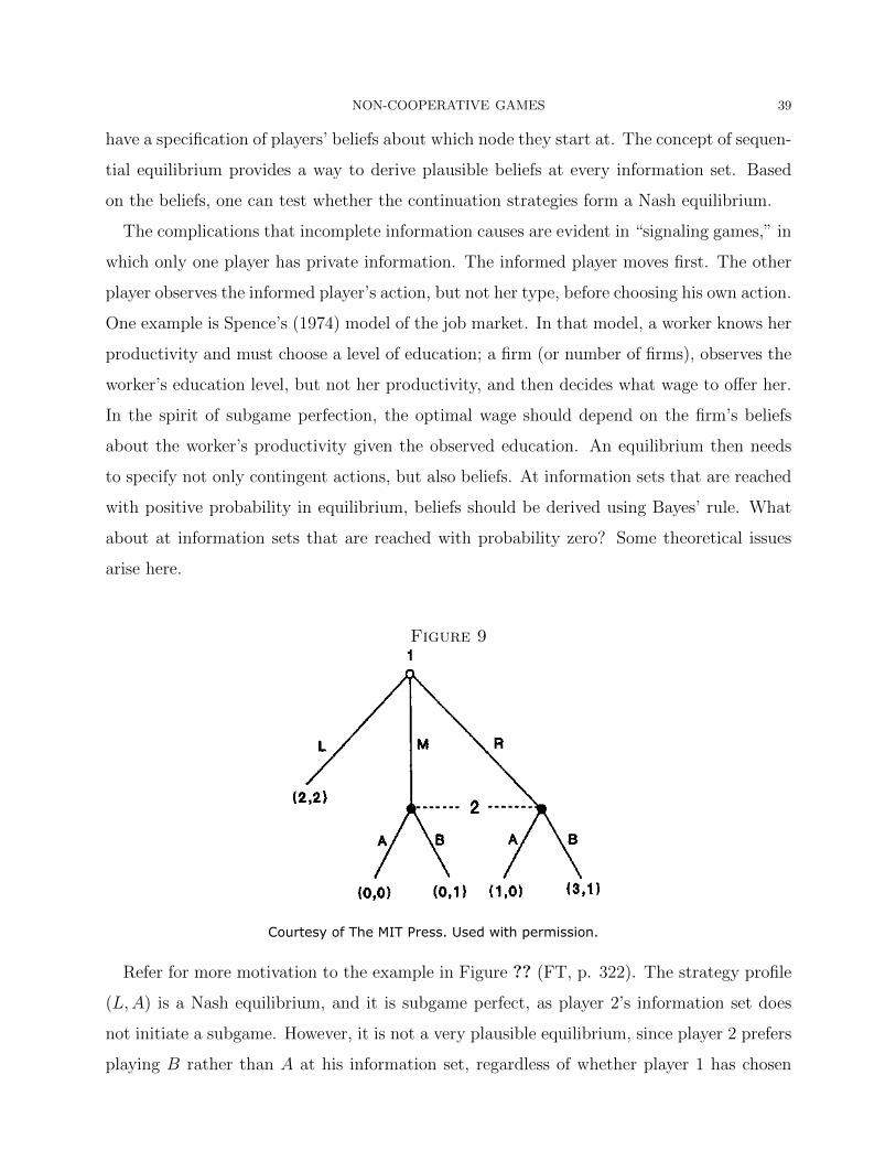
NON-COOPERATIVE GAMES 39
have a specification of players’ beliefs about which node they start at. The concept of sequen-
tial equilibrium provides a way to derive plausible beliefs at every information set. Based
on the beliefs, one can test whether the continuation strategies form a Nash equilibrium.
The complications that incomplete information causes are evident in “signaling games,” in
which only one player has private information. The informed player moves first. The other
player observes the informed player’s action, but not her type, before choosing his own action.
One example is Spence’s (1974) model of the job market. In that model, a worker knows her
productivity and must choose a level of education; a firm (or number of firms), observes the
worker’s education level, but not her productivity, and then decides what wage to offer her.
In the spirit of subgame perfection, the optimal wage should depend on the firm’s beliefs
about the worker’s productivity given the observed education. An equilibrium then needs
to specify not only contingent actions, but also beliefs. At information sets that are reached
with positive probability in equilibrium, beliefs should be derived using Bayes’ rule. What
about at information sets that are reached with probability zero? Some theoretical issues
arise here.
Figure 9
Refer for more motivation to the example in Figure ?? (FT, p. 322). The strategy profile
(L,A) is a Nash equilibrium, and it is subgame perfect, as player 2’s information set does
not initiate a subgame. However, it is not a very plausible equilibrium, since player 2 prefers
playing B rather than A at his information set, regardless of whether player 1 has chosen
Courtesy of The MIT Press. Used with permission.
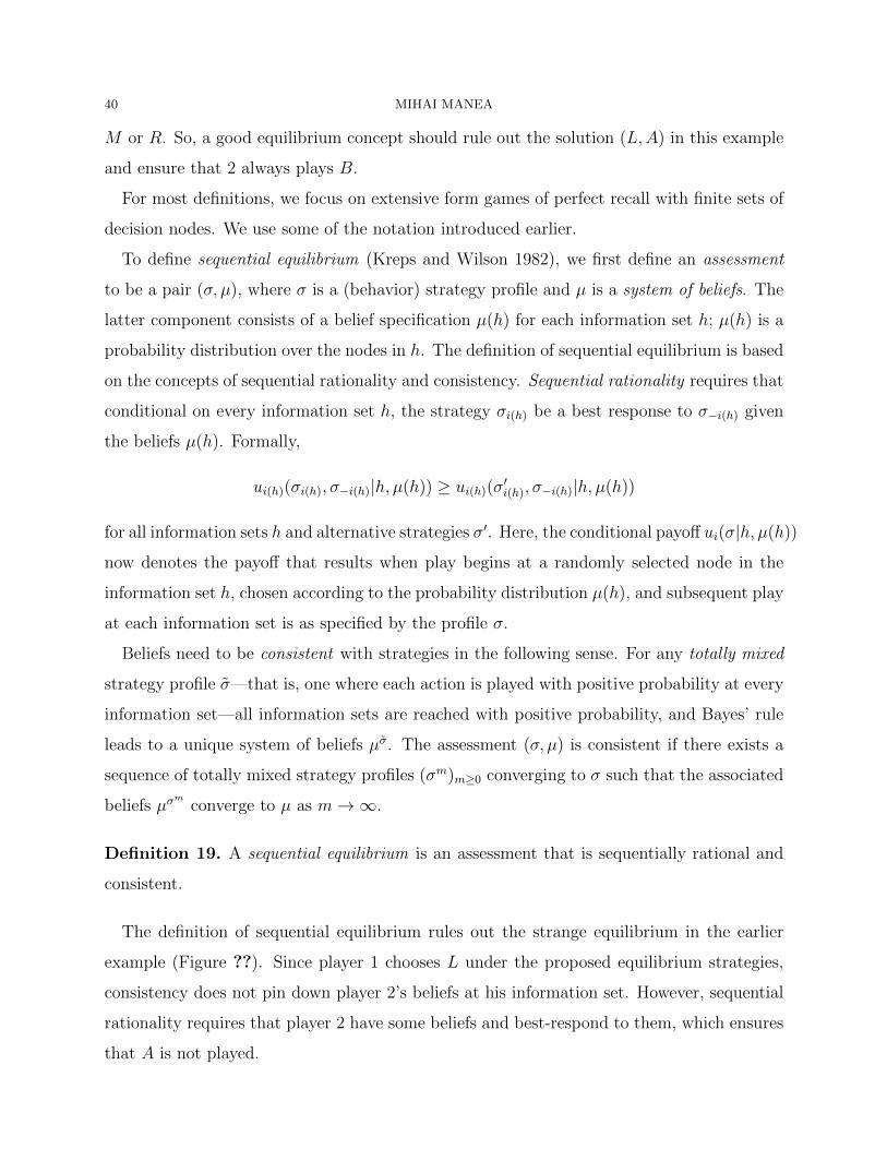
40 MIHAI MANEA
M or R. So, a good equilibrium concept should rule out the solution (L,A) in this example
and ensure that 2 always plays B.
For most definitions, we focus on extensive form games of perfect recall with finite sets of
decision nodes. We use some of the notation introduced earlier.
To define sequential equilibrium (Kreps and Wilson 1982), we first define an assessment
to be a pair (σ, µ), where σ is a (behavior) strategy profile and µ is a system of beliefs. The
latter component consists of a belief specification µ(h) for each information set h; µ(h) is a
probability distribution over the nodes in h. The definition of sequential equilibrium is based
on the concepts of sequential rationality and consistency. Sequential rationality requires that
conditional on every information set h, the strategy σi(h) be a best response to σ−i(h) given
the beliefs µ(h). Formally,
ui(h)(σi(h), σ i(h)|h, µ(h)) ≥ ui(h)(σi′(h), σ h,− −i(h)| µ(h))
for all information sets h and alternative strategies σ′. Here, the conditional payoff ui(σ|h, µ(h))
now denotes the payoff that results when play begins at a randomly selected node in the
information set h, chosen according to the probability distribution µ(h), and subsequent play
at each information set is as specified by the profile σ.
Beliefs need to be consistent with strategies in the following sense. For any totally mixed
strategy profile σ—that is, one where each action is played with positive probability at every
information set—all information sets are reached with positive probability, and Bayes’ rule
leads to a unique system of beliefs µσ. The assessment (σ, µ) is consistent if there exists a
sequence of totally mixed strategy profiles (σm)m 0 converging to σ such that the associated≥
beliefs µσm
converge to µ as m→∞.
Definition 19. A sequential equilibrium is an assessment that is sequentially rational and
consistent.
The definition of sequential equilibrium rules out the strange equilibrium in the earlier
example (Figure ??). Since player 1 chooses L under the proposed equilibrium strategies,
consistency does not pin down player 2’s beliefs at his information set. However, sequential
rationality requires that player 2 have some beliefs and best-respond to them, which ensures
that A is not played.
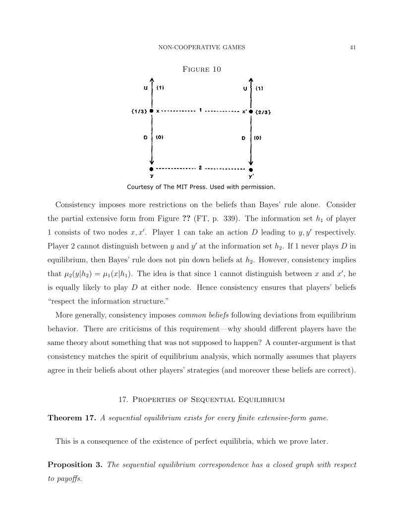
NON-COOPERATIVE GAMES 41
Figure 10
Consistency imposes more restrictions on the beliefs than Bayes’ rule alone. Consider
the partial extensive form from Figure ?? (FT, p. 339). The information set h1 of player
1 consists of two nodes x, x′. Player 1 can take an action D leading to y, y′ respectively.
Player 2 cannot distinguish between y and y′ at the information set h2. If 1 never plays D in
equilibrium, then Bayes’ rule does not pin down beliefs at h2. However, consistency implies
that µ2(y|h2) = µ1(x|h1). The idea is that since 1 cannot distinguish between x and x′, he
is equally likely to play D at either node. Hence consistency ensures that players’ beliefs
“respect the information structure.”
More generally, consistency imposes common beliefs following deviations from equilibrium
behavior. There are criticisms of this requirement—why should different players have the
same theory about something that was not supposed to happen? A counter-argument is that
consistency matches the spirit of equilibrium analysis, which normally assumes that players
agree in their beliefs about other players’ strategies (and moreover these beliefs are correct).
17. Properties of Sequential Equilibrium
Theorem 17. A sequential equilibrium exists for every finite extensive-form game.
This is a consequence of the existence of perfect equilibria, which we prove later.
Proposition 3. The sequential equilibrium correspondence has a closed graph with respect
to payoffs.
Courtesy of The MIT Press. Used with permission.
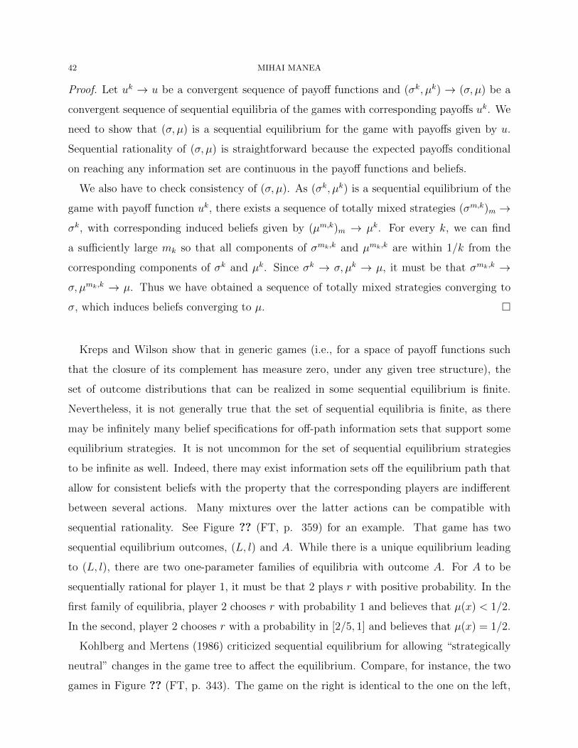
42 MIHAI MANEA
Proof. Let uk → u be a convergent sequence of payoff functions and (σk, µk) → (σ, µ) be a
convergent sequence of sequential equilibria of the games with corresponding payoffs uk. We
need to show that (σ, µ) is a sequential equilibrium for the game with payoffs given by u.
Sequential rationality of (σ, µ) is straightforward because the expected payoffs conditional
on reaching any information set are continuous in the payoff functions and beliefs.
We also have to check consistency of (σ, µ). As (σk, µk) is a sequential equilibrium of the
game with payoff function uk, there exists a sequence of totally mixed strategies (σm,k)m →
σk, with corresponding induced beliefs given by (µm,k)m → µk. For every k, we can find
a sufficiently large m so that all components of σmk,kk and µmk,k are within 1/k from the
corresponding components of σk and µk. Since σk → σ, µk → µ, it must be that σmk,k →
σ, µmk,k → µ. Thus we have obtained a sequence of totally mixed strategies converging to
σ, which induces beliefs converging to µ.
Kreps and Wilson show that in generic games (i.e., for a space of payoff functions such
that the closure of its complement has measure zero, under any given tree structure), the
set of outcome distributions that can be realized in some sequential equilibrium is finite.
Nevertheless, it is not generally true that the set of sequential equilibria is finite, as there
may be infinitely many belief specifications for off-path information sets that support some
equilibrium strategies. It is not uncommon for the set of sequential equilibrium strategies
to be infinite as well. Indeed, there may exist information sets off the equilibrium path that
allow for consistent beliefs with the property that the corresponding players are indifferent
between several actions. Many mixtures over the latter actions can be compatible with
sequential rationality. See Figure ?? (FT, p. 359) for an example. That game has two
sequential equilibrium outcomes, (L, l) and A. While there is a unique equilibrium leading
to (L, l), there are two one-parameter families of equilibria with outcome A. For A to be
sequentially rational for player 1, it must be that 2 plays r with positive probability. In the
first family of equilibria, player 2 chooses r with probability 1 and believes that µ(x) < 1/2.
In the second, player 2 chooses r with a probability in [2/5, 1] and believes that µ(x) = 1/2.
Kohlberg and Mertens (1986) criticized sequential equilibrium for allowing “strategically
neutral” changes in the game tree to affect the equilibrium. Compare, for instance, the two
games in Figure ?? (FT, p. 343). The game on the right is identical to the one on the left,
NON-COOPERATIVE GAMES 43
Figure 11
except that player 1’s first move is split into two moves in a seemingly irrelevant way. Whereas
(A,L2) can be supported as a sequential equilibrium for the game on the left, the strategy
A is not part of a sequential equilibrium for the one on the right. For the latter game, in
the simultaneous-move subgame following NA, the only Nash equilibrium is (R1, R2), as L1
is strictly dominated by R1 for player 1. Hence the unique sequential equilibrium strategies
for the right-hand game are ((NA,R1), R2). This example demonstrates that eliminating a
strictly dominated strategy affects the set of sequential equilibria.
Figure 12
Note that the sensitivity of sequential equilibrium to the addition of “irrelevant moves”
is not a direct consequence of consistency, but is rather implied by sequential rationality.
In the example above, the problem arises even for subgame perfect equilibria. Kohlberg
and Mertens (1986) further develop these ideas in their concept of a stable equilibrium.
However, their criticism that good mistakes should be much more likely than bad mistakes
is not necessarily compelling. If we take seriously the idea that players make mistakes at
each information set, then it is not clear that the two extensive forms in the above example
Courtesy of The MIT Press. Used with permission.
Courtesy of The MIT Press. Used with permission.
44 MIHAI MANEA
are equivalent. In the game on the right, if player 1 makes the mistake of not playing A, he
is still able to ensure that R1 is more likely than L1; in the game on the left, he might take
either action by mistake when intending to play A.
18. Perfect Bayesian Equilibrium
Perfect Bayesian equilibrium was the original solution concept for extensive-form games
with imperfect information, when subgame perfection does not have enough force. It in-
corporated the ideas of sequential rationality and Bayesian updating of beliefs. Nowadays
sequential equilibrium (which was invented later) is the preferred way of expressing these
ideas, but it’s worthwhile to know about PBE since older papers refer to it.
The idea is similar to sequential equilibrium but with simpler requirements about how
beliefs are updated. Fudenberg and Tirole (1991) have a paper that describes various for-
mulations of PBE. The basic requirements are that strategies should be sequentially rational
and that beliefs should be derived from Bayes’ rule wherever applicable, with no constraints
on beliefs at information sets reached with probability zero in equilibrium.
PBE is tipically applied to multi-stage games with incomplete information in which nature
assigns types to players and player actions are observed at the end of every stage. Here are
some other restrictions that can be imposed for such games.
• If player types are drawn independently by nature, beliefs about different players
should remain independent at each history.
• Updating should be “consistent”: given a probability-zero history ht at time t, at
which strategies call for a positive-probability transition to history ht+1, the beliefs
at ht+1 should be given by updating beliefs at ht via Bayes’ rule.
• “Not signaling what you don’t know”: in multi-stage games with independent types,
beliefs about player i at the beginning of period t+ 1 depend only on ht and action
by player i at time t, not also on other players’ actions at time t.
• Two different players i, j should have the same belief about a third player k even at
probability-zero histories.
All of these conditions are implied by consistency.

NON-COOPERATIVE GAMES 45
Anyhow, there does not seem to be a single clear definition of PBE in the literature.
Different sets of conditions are imposed by different authors. This is one more reason why
using sequential equilibrium is preferable.
19. Perfect Equilibrium
Now consider the following game:
L R
U 1, 1 0, 0
D 0, 0 0, 0
Both (U,L) and (D,R) are sequential equilibria (sequential equilibrium coincides with
Nash equilibrium in a strategic-form game). But (D,R) seems non-robust: if player 1 thinks
that player 2 might make a mistake and play L with some small probability, he would rather
deviate to U . This motivates the definition of (trembling-hand) perfect equilibrium (Selten,
1975) for strategic-form games. A profile σ is a PE if there is a sequence of “trembles”
σm → σ, where each σm is a totally mixed strategy, such that σi is a best reply to σm−i for
each m and all i ∈ N .
An equivalent approach is to define a strategy profile σε to be an ε-perfect equilibrium
if there exist ε(si) ∈ (0, ε) for all i and si ∈ Si such that σε is a Nash equilibrium of the
game where players are restricted to play mixed strategies in which every pure strategy si
has probability at least ε(si). A PE is a profile that is a limit of some sequence of ε-perfect
equilibria σε as ε→ 0. (We will not show the equivalence here but it’s not too hard.)
Theorem 18. Every finite strategic-form game has a perfect equilibrium.
Proof. For any ε > 0, we can certainly find a Nash equilibrium of the modified game, where
each player is restricted to play mixed strategies that place probability at least ε on every
pure strategy. (Just apply the usual Nash existence theorem for compact strategy sets and
quasiconcave payoffs.) By compactness, there is some subsequence of these strategy profiles
as ε→ 0 that converges, and the limit point is a perfect equilibrium by definition.
We would like to extend this definition to extensive-form games. Consider the game in
Figure ?? (FT, p. 353). They show an extensive-form game and its reduced normal form.

46 MIHAI MANEA
Figure 13
There is a unique SPE (L1L′1, L2). But (R1, R2) is a PE of the reduced normal form. Thus
perfection in the normal form does not imply subgame-perfection. The perfect equilibrium
is sustained only by trembles such that, conditional on trembling to L1 at the first node,
player 1 is also fairly likely to play R1′ rather than L′1 at his second node. This seems
unreasonable—R1′ is only explainable as a tremble. Perfect equilibrium as defined so far
thus has the disadvantage of allowing correlation in trembles at different information sets.
The solution to this is to impose perfection in the agent-normal form. We treat the two
different nodes of player 1 as being different players, thus requiring them to tremble inde-
pendently. More formally, in the agent-normal form game, we have a player corresponding
to every information set. Given a strategy profile in this game, the “player” corresponding
to any information set h enjoys the same payoffs as player i(h) under the corresponding
strategies in the extensive-form game. Thus, the game in Figure ?? turns into a three-player
game. The only perfect equilibrium of this game is (L1, L′1, L2).
More generally, a perfect equilibrium for an extensive form game is defined to be a perfect
equilibrium of the corresponding agent-normal form.
Courtesy of The MIT Press. Used with permission.
NON-COOPERATIVE GAMES 47
Theorem 19. Every PE of a finite extensive-form game is a sequential equilibrium (for
some appropriately chosen beliefs).
Proof. Let σ be a PE of the extensive-form game. Then there exist totally mixed strategy
profiles in the agent normal form game σm → σ such that σ mh is a best reply to σ−h for each
m and all information sets h. For each σm we have a well-defined belief system µm induced
by Bayes’ rule. Pick a subsequence for which these belief systems converge to some µ. Then
by definition (σ, µ) is consistent. Sequential rationality follows exactly from the fact that
σh is a best reply given µm(·|h) and σm−h for each m along the subsequence, and hence also
with respect to the limit beliefs µ(·|h) and strategies σ h. (More properly, perfection implies−
that there are no one-shot deviations that benefit any player; by an appropriate adaptation
of the one-shot deviation principle we infer that σ is in fact sequentially rational at every
information set.)
The converse is not true—not every sequential equilibrium is perfect, as we already saw
with the simple strategic-form example above. But for generic payoffs it is true (Kreps and
Wilson, 1982).
The set of perfect equilibrium outcomes does not have a closed graph (unlike sequential
or subgame-perfect equilibrium). Consider the following game:
L R
U 1, 1 0, 0
D 0, 0 1/n, 1/n
It has (D,R) as a perfect equilibrium for each n > 0, but in the limit where (D,R) has
payoffs (0, 0) it is no longer a perfect equilibrium. We can think of this as an order-of-limits
problem: as n → ∞ the trembles against which D and R remain best responses become
smaller and smaller. Thus, whether or not (D,R) is a reasonable prediction in the limiting
game depends on whether we think the approximation error in describing the payoffs is larger
than the players’ probability of trembling or vice versa.
20. Proper Equilibrium
Myerson (1978) considered the notion that when a player trembles, he is still more likely
to play better actions than worse ones. Specifically, a player’s probability of playing the
48 MIHAI MANEA
second-best action is at most ε times the probability of the best action, the probability of
the third-best action is at most ε times the probability of the second-best action, and so
forth. Consider the game in Fig. 8.15 of FT (p. 357). (M,M) is a perfect equilibrium,
but Myerson argues that it can be supported only using unreasonable trembles, where each
player has to be likely to tremble to a very bad reply rather than an almost-best reply.
Definition 20. An ε-proper equilibrium is a totally mixed strategy profile σε such that, if
u (s , σε ) < u (s′ , σε εi i i i i i), then σi (si) ≤ εσεi (s
′i). A proper equilibrium is any limit of some− −
ε-proper equilibria as ε→ 0.
Theorem 20. Every finite strategic-form game has a proper equilibrium.
Proof. First prove existence of ε-proper equilibria, using the usual Kakutani argument ap-
plied to the “almost-best-reply” correspondences BRεi rather than the usual best-reply corre-
spondences. (BRεi (σ−i) is the set of mixed strategies for player i in a suitable compact space
of totally mixed strategies that satisfy the inequality in the definiton of ε-proper equilib-
rium.) Then use compactness to show that there exists a sequence that converges as ε→ 0;
its limit is a proper equilibrium.
Given an extensive-form game, a proper equilibrium of the corresponding normal form is
automatically subgame-perfect; we don’t need to go to the agent-normal form. We can show
this by a backward-induction-type argument.
Kohlberg and Mertens (1986) showed that a proper equilibrium in a strategic-form game
is sequential in every extensive-form game having the given normal form. However, it will
not necessarily be a trembling-hand perfect equilibrium in (the agent-normal form of) every
such game. See Figure ?? (FT, p. 358): (L, r) is proper (and so sequential) in the normal
form but not perfect in the agent-normal form.
21. Forward Induction
The preceding ideas are all attempts to capture some kind of forward induction: players
should believe in the rationality of their opponents, even after observing a deviation; thus if
you observe an out-of-equilibrium action being played, you should believe that your opponent
expected you to respond in a way such that his action was reasonable, and this in turn is

NON-COOPERATIVE GAMES 49
Figure 14
informative about his type (or, in more general extensive forms, about how he plans to play
in the future). Forward induction is not itself an equilibrium concept, since in equilibrium all
players know that the specified strategies are to be exactly followed; rather, it is an attempt
to describe reasoning by players who are not quite certain about what will be played. It also
is not a single, rigorously defined concept, but rather a vague term for a form of reasoning
about play.
Consider now the extensive-form game as follows: 1 can play O, leading to (2, 2), or I,
leading to the following battle-of-the-sexes game:
T W
T 0, 0 3, 1
W 1, 3 0, 0
There is an SPE in which player 1 first plays O; conditional on playing I, they play the
equilibrium (W,T ). But the following forward-induction argument suggests this equilibrium
is unreasonable: if player 1 plays I, this suggests he is expecting to coordinate on (T,W )
in the battle-of-the-sexes game, so player 2, anticipating this, will play W . If 1 can thus
convince 2 to play W by playing I in the first stage, he can get the higher payoff (3, 1).
This game can also be represented in (reduced) normal form.
T W
O 2, 2 2, 2
IT 0, 0 3, 1
IW 1, 3 0, 0
Courtesy of The MIT Press. Used with permission.
50 MIHAI MANEA
This representation of the game shows a connection between forward induction and strict
dominance. We can rule out IW because it is dominated by O; then the only perfect
equilibrium of the remaining game is (IT,W ) giving payoffs (3, 1). However, (O, T ) can be
enforced as a perfect (in fact a proper) equilibrium in the original strategic-form game.
Kohlberg and Mertens (1986) argue that an equilibrium concept that is not robust to
deletion of strictly dominated strategies is troubling. The above example, together with
other cases of such non-robustness, leads them to define the notion of stable equilibria. It
is a set-valued concept—not a property of an individual equilibrium but of sets of equilib-
ria. Kohlberg and Mertens first argue that a solution concept should meet the following
requirements:
• Iterated dominance: every stable set must contain a stable set of any game obtained
by deleting a strictly dominated strategy.
• Admissibility: no mixed strategy appearing in a stable set assigns positive probability
to a weakly dominated strategy.
• Invariance to extensive-form representation: they define an equivalence relation be-
tween extensive forms and require that any stable set in one game should be stable
in any equivalent game.
Kohlberg and Mertens define strategic stability in a way such that these criteria are satisfied.
Definition 21. A closed set S of NE is strategically stable if it is minimal among sets with the
following property: for every η > 0, there exists ε > 0 such that all choices of ε(si) ∈ (0, ε),
the game where each player i is constrained to play every si with probability at least ε(si)
has a Nash equilibrium which is within distance η of some equilibrium in S.
Any sequence of ε-perturbed games as ε → 0 should have equilibria corresponding to an
equilibrium in S. Notice that we need the minimality property of S to give bite to this
definition—otherwise, by upper hemi-continuity, we know that the set of all Nash equilibria
would be strategically stable, and we get no refinement. The difference with trembling-hand
perfection is that there should be convergence to one of the equilibria in S for any sequence
of perturbations, not just some sequence of perturbations.
Theorem 21. There exists a stable set that is contained in a connected component of the
set of Nash equilibria. Generically, each component of the set of Nash equilibria leads to a
NON-COOPERATIVE GAMES 51
single distribution over outcomes, so there exists a stable set that induces a unique outcome
distribution. A stable set contains a stable set of any game obtained by eliminating a weakly
dominated strategy and also of any game obtained by deleting a strategy that is not a best
response to any of the opponents’ strategy profiles in the set (“never a weak best reply”
(NWBR)).
NWBR shows that the concept of stable equilibrium is robust to forward induction: know-
ing that player i will not use a particular strategy is consistent with the equilibrium theories
from the stable set.
Every equilibrium in a stable set has to be a perfect equilibrium. This follows from the
minimality condition—if an equilibrium is not a limiting equilibrium along some sequence
of trembles, then there’s no need to include it in the stable set. But notice, these equilibria
are only guaranteed to be perfect in the normal form, not in the agent-normal form (for a
given extensive-form game). Actually, an example due to Gul proves that there exist stable
sets that do not contain any sequential equilibrium.
Normal form games do not directly capture the reasoning of forward induction. Battigalli
and Siniscalchi (2002) seek a general-purpose definition of forward induction by modeling the
belief revision process explicitly in the context of extensive form games. They are interested
in the epistemic conditions that lead to forward induction.
They propose an epistemic model, with each player having a set Ωi of states of the form
ωi = (si, ti), where si represents player i’s disposition to act and ti represents his disposition
to believe. si specifies his action at each information set h of player i, and ti specifies a
belief gi,h ∈ ∆(Ω i) over states of the other players for each h. We say i is rational at−
state ω if si is a best reply to his beliefs ti at each information set. Let R be the set
of states at which every player is rational. For any event E ⊆ Ω, we can define the set
Bi,h(E) = (s, t) ∈ Ω | gi,h(E) = 1, i.e. the set of states where i is sure that E has
occurred (at information set h). Finally SBi(E) = ∩h reachable given EBi,h(E) denotes the set
of states at which i strongly believes in event E, meaning the set of states at which i would
be sure of E as long as he’s reached an information set that is consistent with E occurring.
Finally, Battigalli and Siniscalchi show that SB(R) identifies forward induction—that is,
in the states of the world where everyone strongly believes that everyone is sequentially
52 MIHAI MANEA
rational, strategies must form a profile that is not ruled out by forward induction arguments
of the sort discussed earlier.
Battigalli and Siniscalchi take this a level further by iterating the strong-beliefs operator—
everyone strongly believes that everyone strongly believes that everyone is rational, and
so forth—and this operator leads to backward induction in games of perfect information;
without perfect information, it leads to iterated deletion of strategies that are never a best
reply. This leads to a formalization of the idea of rationalizability in extensive-form games.
22. Forward Induction in Signaling Games
The NWBR property is a useful way to show that some components of equilibria are not
stable. For instance, Cho and Kreps (1987) developed an equilibrium refinement for signaling
games that is weaker than stability–the intuitive criterion–based on iterated applications of
NWBR. Kohlberg and Mertens (1986) motivated their stability concept by mathematical
properties they deemed desirable and robustness with respect to trembles a la Selten’s perfect
equilibrium. By contrast, Cho and Kreps provided a behavioral foundation based on refining
the set of plausible beliefs in the spirit of Kreps and Wilson’s sequential equilibrium.
In a signaling game, there are two players, a sender S and a receiver R. There is a set T
of types for the sender; the realized type will be denoted by t. p(t) denotes the probability
of type t. The sender privately observes his type t, then sends a message m ∈ M(t). The
receiver observes the message and chooses an action a ∈ A(m). Finally both players receive
payoffs uS(t,m, a), uR(t,m, a); thus the payoffs potentially depend on the true type, the
message sent, and the action taken by the receiver. A signaling game is parameterized by
the set T , the prior p, the feasible message and action correspondences M,A, and the payoff
functions uS, uR. In such a game we will use T (m) to denote the set t | m ∈M(t).
Cho and Kreps’ intuitive criterion provides a behavioral explanation of one aspect of the
NWBR property: robustness to replacing the equilibrium path by its expected payoff. This
solution presumes that players are certain about play along the equilibrium path, but there
is uncertainty about play off the path. If we begin with a stable set and then, using NWBR,
delete a strategy in which type t plays an action m, the reduced game should have a stable
component contained in the original component. This means that the surviving equilibria
should assign probability zero to type t following message m.

NON-COOPERATIVE GAMES 53
Consider the beer-quiche signaling game from Figure ?? (FT, p. 450). In this example,
player 1 is wimpy or surly, with respective probabilities 0.1 or 0.9. Player 2 is a bully who
would like to fight the wimpy type but not the surly one. Player 1 orders breakfast and 2
decides whether to fight him after observing his breakfast choice. In the notation above,
T = weak, surly;M = M(t) = beer, quiche, ∀t ∈ T ;A(m) = fight, not fight, ∀m ∈
M .
Figure 15
Player 1 gets a utility of 1 from having his favorite breakfast—beer if surly, quiche if
weak—but a disutility of 2 from fighting. When player 1 is weak, player 2’s utility is 1 if he
fights and 0 otherwise; when 1 is surly, the payoffs to the two actions are reversed.
One can show that all equilibria involve pooling. The key idea in this game is to compare
σ2(F |beer) and σ2(F |quiche). The breakfast leading to a smaller probability of fighting must
be selected with probability 1 in equilibrium by the type of player 1 who likes it. . . We find
that there are two classes of sequential equilibria, corresponding to two distinct outcomes.
In one set of sequential equilibria, both types of player 1 drink beer, while in the other both
types of player 1 eat quiche. In both cases, player 2 must fight with probability at least
1/2 when observing the out-of-equilibrium breakfast since otherwise one of the two types of
player 1 would want to deviate to the other breakfast. Note that either type of equilibrium
can be supported with any belief for player 2 placing a probability weight of at least 1/2 on
player 1 being wimpy following the out-of-equilibrium breakfast (hence there is an infinity
of sequential equilibrium assessments).
Cho and Kreps argued that the equilibrium in which both types choose quiche is unrea-
sonable for the following reason. It does not make any sense for the weak type to deviate
Courtesy of The MIT Press. Used with permission.
54 MIHAI MANEA
to ordering beer, no matter how he thinks that the receiver will react, because he is already
getting payoff 3 from quiche, whereas he cannot get more than 2 from switching to beer.
On the other hand, the surly type can benefit if he thinks that the receiver will react by
not fighting. Thus, conditional on seeing beer ordered, the receiver should conclude that the
sender is surly and so should not want to fight. Clearly, the class of equilibria in which both
types choose quiche violates NWBR.
On the other hand, this argument does not rule out the equilibrium in which both types
drink beer. In this case, in equilibrium the surly type is getting 3, whereas he gets at most
2 from deviating no matter how the receiver reacts; hence he cannot want to deviate. The
weak type, on the other hand, is getting 2, and he can get 3 by switching to quiche if he
thinks this will induce the receiver not to fight him. Thus only the weak type would deviate,
so the sender’s belief (that the receiver is weak if he orders quiche) is reasonable.
Now consider modifying the game by adding an extra option for the receiver: paying
a million dollars to the sender. Now the preceding argument doesn’t rule out the quiche
equilibrium—either type of sender might deviate to beer if he thinks this will induce the
receiver to pay him a million dollars. Hence, in order to apply the same argument, we need
to make the additional assumption that the sender cannot expect the receiver to play a bad
strategy. Then we can restrict attention to the game without the million-dollar option, and
the argument goes through.
Cho and Kreps formalized this line of reasoning in the intuitive criterion, as follows. For
any set of types T ′ ⊆ T and any message m, write
BR(T ′,m) = ∪µ | µ(T ′)=1 BR(µ,m)
—the set of strategies that R could rationally play if he observes m and is sure that the
sender’s type is in T ′. Now with this notation established, consider any sequential equilib-
rium, and let u∗S(t) be the equilibrium payoff to a sender of type t. Define
T (m) = t | u∗S(t) > max uS(t,m, a)a∈BR(T (m),m)
.
This is the set of types that do better in equilibrium than they could possibly do by sending
m, no matter how R reacts, as long as R is playing a best response to some belief. We then
say that the proposed equilibrium fails the intuitive criterion if there exist a type t′ and a
NON-COOPERATIVE GAMES 55
message m ∈M(t′) such that
u∗S(t′) < min uS(t′,m, a).a∈ ˜BR(T (m)\T (m),m)
In words, the equilibrium fails the intuitive criterion if some type t′ of the sender is getting
less than any payoff he could possibly get by playing m, assuming he could thereby convince
˜the sender that he could not possibly be in T (m).
In the beer-quiche example, the all-quiche equilibirum fails this criterion: let t′ = surly
˜and m = beer; check that T (m) = weak.
We can apply this procedure repeatedly, giving the iterated intuitive criterion. Given a
proposed equilibrium, we can use the intuitive criterion as above to rule out pairs (t,m)—
types t that cannot conceivably want to send message m. We can then rule out some actions
of the receiver, by requiring that the receiver should best respond to a belief about the types
that have not yet been eliminated given the message. Under the surviving actions, we can
possibly rule out more pairs (t,m), and so forth.
This idea has been further developed by Banks and Sobel (1987). They say that type t′
is infinitely more likely to choose the out-of-equilibrium message m than type t under the
following condition: the set of possible best-replies by the receiver (possibly mixed) that make
t′ strictly prefer to deviate to m is a strict superset of the possible best-replies that make t
weakly prefer to deviate. If this holds, then conditional on observing m, the receiver should
put probability 0 on type t. The analogue of the Intuitive Criterion under this elimination
procedure is known as D1. If we allow t′ to vary across different best replies by the sender,
requiring only that every best response that weakly induced t to deviate would also strictly
induce some t′ to deviate, then this gives criterion D2. We can also apply either of these
restrictions on beliefs to eliminate possible actions by the receiver, and proceed iteratively.
Iterating D2 leads to the equilibrium refinement criterion known as universal divinity.
The motivating application is Spence’s job-market signaling model. With just two types
of job applicant, the intuitive criterion selects the equilibrium where the low type gets the
lowest level of education and the high type gets just enough education to deter the low type
from imitating her. With more types, the intuitive criterion no longer accomplishes this. D1
does manage to uniquely select the socially optimal separating equilibrium by having each
type get just enough education to deter the next-lower type from imitating her.

56 MIHAI MANEA
23. The Spence Signaling Model
We next consider Spence’s (1973) signaling model of the job market.13 An employer faces
a worker of unknown ability θ. The ability of the worker is known to the worker though, and
is either θ = H or θ = L, where H > L > 0. Interpret these numbers as the money value of
what the worker would produce working in the firm.
The worker would like to transmit the knowledge of her ability to the firm; the problem
is how to do so in a credible way. Think of education as just such a device.
23.1. The Game. Specifically, suppose that a worker can choose to acquire e units of edu-
cation, where e is any nonnegative number. Of course, the worker will have to study hard
to obtain her education, and this creates disutility (studying for exams, doing homework,
etc.). Assume that a worker of true ability θ expends e/θ in disutility. The point is, then,
that H-types can acquire education easier than L-types.
The game proceeds as follows:
1. Nature moves and chooses a worker type, H or L. The type is revealed to the worker
but not to the employer.
2. The worker then chooses e units of education. This is perfectly observed by the
employer.
3. The employer observes e and forms an estimate of θ. He then pays the worker a salary
equal to this estimate, which is just the conditional expectation of θ given e, written IE(θ|e).
4. The H-worker’s payoff is IE(θ|e)− e/H, and the L-worker’s payoff is IE(θ|e)− e/L.
The game is set up so simply that the employer’s expected payoff is zero. Essentially, we
assume that the worker’s choice of education is visible to the world at large so that perfect
competition must push her wage to IE(θ|e), the conditional expectation of θ given e.
Very Important. Note well that IE(θ|e) is not just a given but it is an endogenous object
derived from strategies. How it is computed will depend on worker strategies and how they
translate in beliefs.
23.2. Single Crossing. Suppose that a worker of type θ uses a probability distribution µθ
over different education levels. First observe that if e is a possible choice of the high worker
13This exposition is based on notes by Debraj Ray(http://www.econ.nyu.edu/user/debraj/Courses/05UGGameLSE/Handouts/05uggl10.pdf).
NON-COOPERATIVE GAMES 57
and e′ a possible choice of the low worker, then it must be that e ≥ e′. This follows from the
following important single-crossing argument.
The H-type could have chosen e′ instead of e, so
e(23.1) IE(θ|e)−
H≥ IE(θ|e′)− e′
,H
while the L-type could have chosen e instead of e′, so
e′(23.2) IE(θ|e′)−
L≥ IE(θ|e)− e
.L
Adding both sides in (??) and (??), we see that
(e− e′)(
1
L− 1
0H
)≥ .
Because 1/L > 1/H, it follows that e ≥ e′.
Essentially, if the low type weakly prefers a higher education to a lower one, the high type
would strictly prefer it. So a high type can never take strictly less education than a low type
in equilibrium.
This sort of result typically follows from the assumption that being a high type reduces
not just the total cost from taking an action but also the marginal cost of that action; in this
case, of acquiring one more unit of education. As long as this feature is present, we could
replace the cost function e/θ by any cost function and the same analysis goes through.
23.3. Equilibrium. Now that we know that the high type will not invest any less than the
low type, we are ready to describe the equilibria of this model. There are three kinds of
equilibria here; the concepts are general and apply in many other situations.
1. Separating Equilibrium. Each type takes a different action, and so the equilibrium
action reveals the type perfectly. It is obvious that in this case, L must choose e = 0, for
there is nothing to be gained in making a positive effort choice.
What about H? Note: she cannot play a mixed strategy because each of her actions fully
reveals her type, so she might as well choose the least costly of those actions. So she chooses
a single action: call it e∗, and obtains a wage equal to H. Now these are the crucial incentive
constraints; we must have
e∗(23.3) H −
L≤ L,
58 MIHAI MANEA
otherwise the low person will try to imitate the high type, and
e∗(23.4) H − L,
H≥
otherwise the high person will try to imitate the low type.
Look at the smallest value of e∗ that just about satisfies (??); call it e1. And look at
the largest value of e∗ that just about satisfies (??); call it e2. Clearly, e1 < e2, so the two
restrictions above are compatible.
Any outcome in which the low type chooses 0 and the high type chooses some e∗ ∈ [e1, e2]
is supportable as a separating equilibrium. To show this we must also specify the beliefs
of the employer. There is a lot of leeway in doing this. Here is one set of beliefs that
works: the employer believes that any e < e∗ (if observed) comes from the low type, while
any e > e∗ (if observed) comes from the high type. These beliefs are consistent because
sequential equilibrium in this model imposes no restrictions on off-the-equilibrium beliefs.
Given these beliefs and equations (??) and (??), we can check that no type has incentives
to deviate.
2. Pooling Equilibrium. There is also a family of pooling equilibria in which only one
signal is received in equilibrium. It is sent by both types, so the employer learns nothing
new about the types. So if it sees that signal — call it e∗ — it simply pays out the expected
value calculated using the prior beliefs: pH + (1− p)L.
Of course, for this to be an equilibrium two conditions are needed. First, we need to
specify employer beliefs off the equilibrium path. Again, a wide variety of such beliefs are
compatible; here is one: the employer believes that any action e 6= e∗ is taken by the low
type. [It does not have to be this drastic.14] Given these beliefs, the employer will “reward”
any signal not equal to e∗ with a payment of L. So for the types not to deviate, it must be
that
e∗pH + (1− p)L− L,
θ≥
but the binding constraint is clearly for θ = L, so rewrite as
e∗pH + (1− p)L−
L≥ L.
14For instance, the employer might believe that any action e < e∗ is taken by the low type, while any actione > e∗ is taken by types in proportion to their likelihood: p : 1− p.

NON-COOPERATIVE GAMES 59
This places an upper bound on how big e∗ can be in any pooling equilibrium. Any e∗ between
0 and this bound will do.
3. Hybrid Equilibria. There is also a class of “hybrid equilibria” in which one or both
types randomize. For instance, here is one in which the low type chooses 0 while the high
type randomizes between 0 (with probability q) and some e with probability 1 − q. If the
employer sees e he knows the type is high. If he sees 0 the posterior probability of the high
type there is — by Bayes’ Rule — equal to
qp,
qp+ (1− p)
and so the employer must pay out a wage of precisely
qp
qp+ (1− p)H +
1− pL.
qp+ (1− p)
But the high type must be indifferent between the announcement of 0 and that of e, because
he willingly randomizes. It follows that
qp
qp+ (1− p)H +
1− pqp+ (1− p)
L = H − e.
H
To complete the argument we need to specify beliefs everywhere else. This is easy as we’ve
seen more than once (just believe that all other e-choices come from low types). We therefore
have a hybrid equilibrium that is “semi-separating”.
In the Spence model all three types of equilibria coexist. Part of the reason for this is that
beliefs can be so freely assigned off the equilibrium path, thereby turning lots of outcomes
into equilibria. What we turn to next is a way of narrowing down these beliefs. To be sure,
to get there we have to go further than just sequential equilibrium.
23.4. The Intuitive Criterion. Consider a sequential equilibrium and a non-equilibrium
announcement (such as an nonequilibrium choice of education in the example above). What
is the other recipient of such a signal (the employer in the example above) to believe when
she sees that signal?
Sequential equilibrium imposes little or no restrictions on such beliefs in signalling models.
[We have seen, of course, that in other situations — such as those involving moves by Nature
— that it does impose several restrictions, but not in the signalling games that we have been
60 MIHAI MANEA
studying.] The purpose of the Intuitive Criterion is to try and narrow beliefs further. In this
way we eliminate some equilibria and in so doing sharpen the predictive power of the model.
Consider some non-equilibrium signal e. Consider some type of a player, and suppose
even if she were to be treated in the best possible way following the emission of the signal
e, she still would prefer to stick to her equilibrium action. Then we will say that signal e is
equilibrium-dominated for the type in question. She would never want to emit that signal,
except purely by error. Not strategically.
The Intuitive Criterion (IC) may now be stated.
If, under some ongoing equilibrium, a non-equilibrium signal is received which is equilibrium-
dominated for some types but not others, then beliefs cannot place positive probability weight
on the former set of types.
Notice that IC places no restrictions on beliefs over the types that are not equilibrium dom-
inated, and in addition it also places no restrictions if every type is equilibrium-dominated.
For then the deviation signal is surely an error, and once that possibility is admitted, all
bets about who is emitting that signal are off.
The idea behind IC is the following “speech” that a sender (of signals) might make to a
recipient:
Look, I am sending you this signal which is equilibrium-dominated for types A, B or C.
But it is not so for types D and E. Therefore you cannot believe that I am types A, B or
C.
Let us apply this idea to the Spence model.
Proposition 4. In the Spence Signalling model, a single equilibrium outcome survives the
IC, and it is the separating equilibrium in which L plays 0 while H plays e1, where e1 solves
(??) with equality.
Proof. First we rule out all equilibria in which types H and L play the same value of e with
positive probability. [This deals with all the pooling and all the hybrid equilibria.]
At such an e, the payoff to each type θ is
eλH + (1− λ)L−
θ,

NON-COOPERATIVE GAMES 61
where λ represents the employer’s posterior belief after seeing e. Now, there always exists
an e′ > e such that
eλH + (1− λ)L−
L= H − e′
L< H − e′
H
If we choose e′′ very close to e′ but slightly bigger than it, it will be equilibrium-dominated
for the low type —
eλH + (1− λ)L−
L> H − e′′
,L
while it is not equilibrium-dominated for the high type:
eλH + (1− λ)L−
H< H − e′′
.H
But now the equilibrium is broken by having the high type deviate to e′′. By IC, the employer
must believe that the type there is high for sure and so must pay out H. But then the high
type benefits from this deviation relative to playing e.
Next, consider all separating equilibria in which L plays 0 while H plays some e > e1.
Then a value of e′ which is still bigger than e1 but smaller than e can easily be seen to
be equilibrium-dominated for the low type but not for the high type. So such values of e′
must be rewarded with a payment of H, by IC. But then the high type will indeed deviate,
breaking the equilibrium.
This proves that the only equilibrium that can survive the IC is the one in which the low
type plays 0 and the high type chooses e1.
The heart of the intuitive criterion is an argument which is more general: it is called
forward induction. The basic idea is that an off-equilibrium signal can be due to one of two
things: an error, or strategic play. If at all strategic play can be suspected, the error theory
must play second fiddle: that’s what a forward induction argument would have us believe.
24. Forward Induction and Iterated Weak Dominance
In the same way that iterated strict dominance and rationalizability can be used to narrow
down the set of predictions without pinning down strategies perfectly, the concept of iterated
weak dominance (IWD) can be used to capture some of the force of forward and backward
induction without assuming that players coordinate on a certain equilibrium. Since the idea
of forward induction is that players interpret a deviation as a signal of future play, forward
62 MIHAI MANEA
induction is more compatible with a situation of considerable strategic uncertainty–a non-
equilibrium model-rather than a theory in which players are certain about the opponents’
strategies.
In games with perfect information iterated weak dominance implies backward induction.
Indeed, any suboptimal strategy at a penultimate node is weakly dominated, then we can
iterate this observation.
IWD also captures part of the forward induction notion implicit in stability, since stable
components contain stable sets of games obtained by removing a weakly dominated action.
For instance, applying IWD to the motivating example of Kohlberg and Mertens we obtain
T W
O 2, 2 2, 2
IT 0, 0 3, 1
IW 1, 3 0, 0
the unique outcome (IT,W ) predicted by stability.
Similarly, we can solve the beer-quiche game using IWD. Consider the ex ante game in
which the types of player 1 are treated as two distinct information sets for the same player.
Player 1’s strategy (beer if wimp, quiche if surly) is strictly dominated by a strategy under
which with probability .9 both types of player 1 eat quiche and with probability .1 both
drink beer. Indeed, for any strategy of player 2, the latter strategy involves the same total
probability that player 1 is fought by player 2 as the former, but the latter leads to player 1’s
favorite breakfast with higher probability. Once we eliminate (beer if wimp, quiche if surly),
only the strategies (beer if wimp, beer if surly) and (quiche if wimp, beer if surly) generate
a breakfast of beer for player 1. Then the decision of whether player 2 should fight after
observing a breakfast of beer makes a difference only in the event that player 1 uses one of
these two strategies. The best response to either strategy is not fighting because it implies
a probability of at least .9 of confronting the surly type. This means that any strategy for
2 that involves fighting after observing beer is weakly dominated in the strategic form by
one with no fighting after beer. Then the surly type should choose beer in any surviving
equilibrium, which generates his highest possible payoff of 3–he has his preferred breakfast
and is not challenged by player 2.
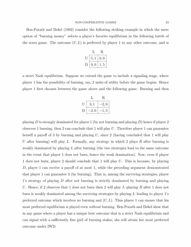
NON-COOPERATIVE GAMES 63
Ben-Porath and Dekel (1992) consider the following striking example in which the mere
option of “burning money” selects a player’s favorite equilibrium in the following battle of
the sexes game. The outcome (U,L) is preferred by player 1 to any other outcome, and is
L R
U 5, 1 0, 0
D 0, 0 1, 5
a strict Nash equilibrium. Suppose we extend the game to include a signaling stage, where
player 1 has the possibility of burning, say, 2 units of utility before the game begins. Hence
player 1 first chooses between the game above and the following game. Burning and then
L R
U 3, 1 −2, 0
D −2, 0 −1, 5
playing D is strongly dominated for player 1 (by not burning and playing D) hence if player 2
observes 1 burning, then 2 can conclude that 1 will play U . Therefore player 1 can guarantee
herself a payoff of 3 by burning and playing U , since 2 (having concluded that 1 will play
U after burning) will play L. Formally, any strategy in which 2 plays R after burning is
weakly dominated by playing L after burning (the two strategies lead to the same outcome
in the event that player 1 does not burn, hence the weak domination). Now, even if player
1 does not burn, player 2 should conclude that 1 will play U . This is because, by playing
D, player 1 can receive a payoff of at most 1, while the preceding argument demonstrated
that player 1 can guarantee 3 (by burning). That is, among the surviving strategies, player
1’s strategy of playing D after not burning is strictly dominated by burning and playing
U . Hence, if 2 observes that 1 does not burn then 2 will play L–playing R after 1 does not
burn is weakly dominated among the surviving strategies by playing L–leading to player 1’s
preferred outcome which involves no burning and (U,L). Thus player 1 can ensure that his
most preferred equilibrium is played even without burning. Ben-Porath and Dekel show that
in any game where a player has a unique best outcome that is a strict Nash equilibrium and
can signal with a sufficiently fine grid of burning stakes, she will attain her most preferred
outcome under IWD.
64 MIHAI MANEA
25. Repeated Games
We now move on to consider another important topic: repeated games. Let G = (N,A, u)
be a normal-form stage game. At time t = 0, 1, . . ., the players simultaneously play game
G. At each period, the players can all observe play in each previous period; the history
is denoted ht = (a0, . . . , at−1). Payoffs in the repeated game RG(δ) are given by Ui =
(1− δ)∑∞
t=0 δtui(a
t). The (1− δ) factor normalizes the sum so that payoffs in the repeated
game are on the same scale as in the stage game. We assume players follow behavior strategies
(by Kuhn’s theorem), so a strategy σi for player i is given by a choice of σi(ht) ∈ ∆(Ai) for
each history ht. Given such strategies, we can define continuation payoffs after any history
ht: U (σ|hti ).
If α∗ is a Nash equilibrium of the static game, then playing α∗ at every history is a
subgame-perfect equilibrium of the repeated game. Conversely: for any finite game G and
¯ ¯any ε > 0, there exists δ with the property that, for any δ < δ, any SPE of the repeated game
RG(δ) has the property that, at every history, play is within ε of a static NE (in the strategy
space). However, interesting results generally occur when players have high discount factors,
not low discount factors.
The main results for repeated games are “Folk Theorems”: for high enough δ, every feasible
and individually rational payoff vector in the stage game can be attained in an equilibrium
of the repeated game. There are several versions of such a theorem, which is why we use
the plural. For now, we look at repeated games with perfect monitoring (the class of games
defined above), where the appropriate equilibrium concept is SPE. We can check if a strategy
profile is an SPE by using the one-shot deviation principle. Conditional on a history ht, i’s
payoff from playing a and then following σ in the continuation is given by the value function
(25.1) Vi(a) = (1− δ)ui(a) + δUi(σ|ht, a).
This gives us an easy way to check whether or not a player wants to deviate from a proposed
strategy, given other player’s strategies. σ is an SPE if and only if, for every history ht, σ|ht
is a NE of the induced game G(ht, σ) whose payoffs are given by (??).
To state a folk theorem, we need to explain the terms “individually rational” and “feasi-
ble.” The minmax payoff of player i is the worst payoff his opponents can hold him down

NON-COOPERATIVE GAMES 65
to if he knows their strategies:
vi = ∏min
[max ui(ai, α−i)
α−i∈ ∆(A aj 6 i j) i=
∈Ai
].
We will let mi, a minmax profile for i, denote a profile of strategies (ai, α i) that solves−
this minimization and maximization problem. Note that we require independent mixing
by i’s opponents. It is important to consider mixed, rather than just pure, strategies for
i’s opponents. For instance, in the matching pennies game the minmax when only pure
strategies are allowed for the opponent is 1, while the actual minmax, involving mixed
strategies, is 0.
In any SPE—in fact, any Nash equilibrium—i’s payoff is at least his minmax payoff, since
he can always get at least this much by just best-responding to his opponents’ (possibly
independently mixed) actions in each period separately. This motivates us to say that a
payoff vector v (i.e. an element of RN , specifying a payoff for each player) is individually
rational if vi ≥ vi for each i, and it is strictly individually rational if the inequality is strict
for each i.
The set of feasible payoffs (properly, feasible payoff vectors) is the convex hull of the
set u(a) | a ∈ A. Again note that this can include payoffs that are not obtainable in the
stage game using mixed strategies, because some such payoffs may require correlation among
players to achieve. Under the common discount factor assumption, the normalized payoffs
along any path of play in the repeated game are certainly in the feasible set.
Also, in studying repeated games we usually assume the availability of a public random-
ization device that produces a publicly observed signal ωt ∈ [0, 1], uniformly distributed and
independent across periods, so that players can condition their actions on the signal. Prop-
erly, we should include the signals (or at least the current period’s signal) in the specification
of the history, but it is conventional not to write it out explicitly. The public randomization
device is a convenient way to convexify the set of possible equilibrium payoff vectors: for
example, given equilibrium payoff vectors v and v′, any convex combination of them can be
realized by playing the equilibrium with payoffs v conditional on some realizations of the
device and v′ otherwise. (Fudenberg and Maskin (1991) showed that one can actually do

66 MIHAI MANEA
this without the public randomization device for sufficiently high δ, while preserving incen-
tives, by appropriate choice of which periods to play each action profile involved in any given
convex combination.)
An easy folk theorem is that of Friedman (1971):
Theorem 22. If e is the payoff vector of some Nash equilibrium of G, and v is a feasible
payoff vector with vi > ei for each i, then for all sufficiently high δ, there exists an SPE with
payoffs v.
Proof. Just specify that the players play whichever action profile gives payoffs v (using the
public randomization device to correlate their actions if necessary), and revert to the static
Nash permanently if anyone has ever deviated. When δ is high enough, the threat of reverting
to Nash is severe enough to deter anyone from deviating.
So, in particular, if there is a Nash equilibrium that gives everyone their minmax payoff
(for example, in the prisoner’s dilemma), then every strictly individually rational and feasible
payoff vector is obtainable in SPE.
However, it would be nice to have a full, or nearly full, characterization of the set of
possible equilibrium payoff vectors (for large δ). In many repeated games, the Friedman folk
theorem is not strong enough for this. A more general folk theorem would say that every
individually rational, feasible payoff is achievable in SPE under general conditions. This is
harder to show, because in order for one player to be punished by minmax if he deviates,
others need to be willing to punish him. Thus, for example, if all players have equal payoff
functions, then it may not be possible to punish a player for deviating, because the punisher
hurts himself as well as the deviator.
For this reason, the standard folk theorem (due to Fudenberg and Maskin, 1986) requires
a full-dimensionality condition.
Theorem 23. Suppose the set of feasible payoffs has full dimension n. For any feasible and
strictly individually rational payoff vector v, there exists δ such that whenever δ > δ, there
exists an SPE of RG(δ) with payoffs v.
Actually we don’t quite need the full-dimensionality condition—all we need, conceptually,
is that there are no two players who have the same payoff functions; more precisely, no
NON-COOPERATIVE GAMES 67
player’s payoff function can be a positive affine transformation of any other’s (Abreu, Dutta,
and Smith, 1994). But the proof is easier under the stronger assumption.
Proof. We will first give the construction assuming that i’s minmax action profile mi is pure.
Consider the action profile a for which u(a) = v. Choose v′ in the interior of the feasible,
individually rational set with v ii′ < vi for each i. Let w denote v′ with ε added to each
player’s payoff except for player i; with ε low enough, this will again be a feasible payoff
vector.
Strategies are now specified as follows.
• Phase I: play a, as long as there are no deviations. If i deviates, switch to IIi.
• Phase II ii: play m . If player j deviates, switch to IIj. (If several players deviate
simultaneously, we may arbitrarily choose j among them; this makes little difference,
since verification of the equilibrium will only require checking single deviations.) Note
that if mi is a pure strategy profile it is clear what we mean by j deviating. If it
requires mixing it is not so clear; this will be discussed in the second part of the
proof. Phase IIi lasts for T periods, where T is a number, independent of δ, to be
determined, and if there are no deviations during this time, play switches to IIIi.
• Phase III ii: play the action profile leading to payoffs w forever. If j deviates, go to
IIj. (This is the “reward” phase that gives players −i incentives to punish in phase
IIi.)
We check that there are no incentives to deviate, using the one-shot deviation principle
for each of the three phases: calculate the payoff to i from complying and possible deviations
in each phase. Phases IIi and IIj (j 6= i) need to be considered separately, as do IIIi and
IIIj.
• Phase I: deviating gives at most (1− δ)M + δ(1− δT )v Ti + δ +1vi
′, where M is some
upper bound on all of i’s feasible payoffs, and complying gives vi. Whatever T we
have chosen, it is clear that as long as δ is sufficiently close to 1, complying produces
a higher payoff than deviating, since vi′ < vi.
• Phase IIi: Suppose there are T ′ ≤ T remaining periods in this phase. Then complying
gives i a payoff of (1 − δT ′)v Ti + δ
′vi′, whereas since i is being minmaxed, deviating
can’t help in the current period and leads to T more periods of punishment, for a
68 MIHAI MANEA
total payoff of at most (1 − δT+1)v Ti + δ +1vi
′. Thus deviating is always worse than
complying.
• Phase II : With T ′ remaining periods, i gets (1 − δT′
j )ui(mj) + δT
′(vi′ + ε) from
complying and at most (1− δ)M + (δ − δT+1)v Ti + δ +1vi
′ from deviating. When δ is
large enough, complying is preferred.
• Phase IIIi: This is the one case that affects the choice of T . Complying gives vi′
in every period, while deviating gives at most (1 − δ)M + δ(1 − δT )v Ti + δ +1vi
′.
Rearranging, the comparison is between (δ + δ2 + . . .+ δT )(vi′ − vi) and M − v′i. For
any δ ∈ (0, 1), there exists T such that the desired inequality holds for all δ > δ.
• Phase IIIj: Complying gives vi′ + ε forever, whereas deviating leads to a switch to
phase IIi and so gives at most (1− δ)M + δ(1− δT )v Ti+ δ +1vi
′. Again, for sufficiently
large δ, complying is preferred.
Now we need to deal with the part where minmax strategies are mixed. For this we need to
change the repeated-game strategies so that, during phase IIj, player i is indifferent among
all the possible sequences of T realizations of his prescribed mixed action. We accomplish
this by choosing a different reward ε for each such sequence, so as to balance out their
different short-term payoffs. We’re not going to talk about this in detail; see the Fudenberg
and Maskin paper for this.
26. Repeated Games with Fixed δ < 1
The folk theorem shows that many payoffs are possible in SPE. But the construction of
strategies in the proof is fairly complicated, since we need to have punishments and then
rewards for punishers to induce them not to deviate. In general, an equilibrium may be
supported by an elaborate hierarchy of punishments, and punishments of deviations from
the prescribed punishments, and so on. Also, the folk theorem is concerned with limits as
δ → 1, whereas we may be interested in the set of equilibria for a particular value of δ < 1.
We will now approach the question of identifying equilibrium payoffs for a given δ < 1.
In repeated games with perfect information, it turns out that an insight of Abreu (1988)
will simplify the analysis greatly: equilibrium strategies can be enforced by using a worst
possible punishment for any deviator. First we need to show that there is a well-defined
worst possible punishment.
NON-COOPERATIVE GAMES 69
Theorem 24. Suppose each player’s action set in the stage game is a compact subset of a
Euclidean space and payoffs are continuous in actions, and some pure-strategy SPE of the
repeated game exists. Then, among all pure-strategy SPEs, there is one that is worst for
player i.
That is, the infimum of player i’s payoffs, across all pure-strategy SPEs, is attained.
Proof. We prove this for every player i simultaneously.
An equilibrium play path is an infinite sequence of action profiles, one for each period, that
is attained in some pure-strategy SPE. Fix a sequence of such play paths ai,k, k = 0, 1, 2, . . .
such that Ui(ai,k) converges to the specified infimum y(i), as k → ∞. We want to define a
limit of the play paths, in such a way that the limiting path is again achieved in some SPE,
with payoff y(i) to player i. The constructed equilibria rely on each other for punishments
off the equilibrium path.
Each play path is an element of the strategy space∏
t 0A, where A is the action space of≥
the stage game. Endow this space with the product topology. Convergence in the product
topology is defined componentwise—that is, ai,k → ai,∞ if and only if ai,kt → ai,t∞ for each
t. Because the space of paths is sequentially compact,15 by passing to a subsequence if
necessary, we can ensure that the ai,k have a limiting play path ai,∞. It is easy to check that
the resulting payoff to player i is y(i).
Now we just have to check that this limiting play path ai,∞ is supportable as an SPE
by some strategy profile. We construct the following profile. Play starts in regime i. A
deviation by player j from the current regime leads to regime j. In each regime i, all players
play according to ai,∞.
15By a diagonalisation argument, a countable product of sequentially compact spaces is sequentially compact.Note that while the set of play paths in Abreu’s setting is sequentially compact, the space of pure strategyprofiles is not. This space is an uncountable product of Euclidean sets. For instance, second-period strategiesdepend on the first period action profile and are represented by the set AA. Even when A is an closed interval,AA is not sequentially compact. (Note, however, that by Tychonoff’s theorem AA is a compact set.) Fora proof, consider the set [0, 1][0,1] with the product topology. We can think of each point in the set as afunction f : [0, 1]→ [0, 1]. Convergence in the product topology reduces to point-wise convergence for suchfunctions. Let fn(x) denote the nth digit in the binary expansion of x. The sequence (fn) does not admit aconvergent subsequence. Indeed, for any subsequence (fnk
)k≥0 consider an x ∈ [0, 1] whose binary expansionhas the nk entry equal to 0 for k even and 1 for k odd. Then (fnk
(x))k 0 is not a convergent sequence of≥real numbers, and hence (fnk
)k≥0 does not converge in the product topology.
70 MIHAI MANEA
Now we need to check that the |N | strategy profiles constructed this way are indeed SPEs.
Consider a deviation by player j from stage τ of regime i to an action aj. His payoff from
deviating is
i,
(1− δ)uj(aj, a ∞j (τ)) + δy(j).−
We want to show that this is at most the continuation payoff from complying,
∞
(1− δ)∑
δtuj(ai,∞(τ + t)).
t=0
But we know that for each k, there is some SPE whose equilibrium play path is ai,k; in SPE,
j is disincentivized from deviating, and we also know that by deviating his value in future
periods is at least y(j) (by definition of y(j)). So for each k we have
∞
(1− δ)∑
δtuj(ai,k(τ + t)) ≥ uj(aj, a
i,k +−j(τ)) δy(j).t=0
By taking limits at k →∞, we see that there is no incentive to deviate in the strategy profile
supporting ai,∞, either.
This shows there are never incentives for a one-shot deviation. So by the one-shot deviation
principle, we do have an SPE giving i his infimum of SPE payoffs, for each player i.
Abreu refers to an SPE that gives i his worst possible payoff as an optimal penal code.
The above theorem applies when there exists a pure-strategy SPE. If the stage game is
finite, there frequently will not be any pure-strategy SPE. In this case, there will be mixed-
strategy SPE, and we would like to again prove that an optimal (mixed-strategy) penal code
exists. A different method is required; we invoke a theorem of Fudenberg and Levine (1983).
Theorem 25. Consider an infinite-horizon repeated game with a finite stage game. The
set of strategy profiles is simply the countable product ht i ∆(Ai), taken over all possible
finite histories ht and players i. Put the product topology
∏on
∏this space. Then the set of SPE
profiles and payoffs are nonempty and compact.
The set of SPEs in nonempty because it includes strategies that play the same static Nash
equilibrium following any history. Since the stage game is finite, ht i ∆(Ai) is a countable
product of sequentially compact spaces, so it is sequentially compact
∏ ∏(see also footnote ??).
One can easily show that payoffs vary continuously in the strategy profile for the repeated
NON-COOPERATIVE GAMES 71
game (with the product topology). Indeed, for any sequence σn → σ and any fixed t, the
distribution over date t histories/actions induced by σn converges to the one induced by σ
as n→∞. Then the expected payoffs under σn converge to those under σ as n→∞. This
immediately implies that the set of SPEs is closed.16 Since∏
ht
∏i ∆(Ai) is compact by
Tychonoff’s theorem and closed subsets of compact sets are compact, it follows that the set
of SPE strategies is compact. As payoffs are continuous in strategies, the set of SPE payoffs
is also compact.17 In particular, for every player i there exists an SPE that minimizes i’s
payoff, that is, an optimal penal code for i.
The following result holds in either of the settings where we proved the existence of an
optimal penal code—either for pure strategies when the stage game has continuous action
spaces (and some SPE exists) or for mixed strategies when the stage game is finite.
Theorem 26. (Abreu, 1988) Any distribution over play paths achievable by an SPE can be
generated by an SPE enforced by optimal penal codes off the equilibrium path, i.e. when i is
the first to deviate, continuation play follows the optimal penal code for i.
For mixed-strategy equilibria, “off the path” means “at histories that occur with proba-
bility zero.”
Proof. Let σ be the given SPE. Form a new strategy profile s by leaving play on the equilib-
rium path as proposed by σ, and replacing play off the equilibrium path by the optimal penal
code for i when i is the first deviator (or one of the first deviators, if there is more than one).
By the one-shot deviation principle and the fact that off-path play follows an SPE, we need
only check that i does not want to deviate when play so far is on the equilibrium path—but
this is immediate, because i is punished with y(i) in the continuation if he deviates, whereas
in the original profile σ he would get at least y(i) in the continuation (by definition of y(i))
and we know this was already low enough to deter deviation (because σ was an SPE).
Abreu (1986) looks at symmetric games and considers strongly symmetric equilibria—
equilibria in which all players behave identically at every history, including asymmetric
16Since countable product of metric spaces is metrizable, the product topology on h i ∆(Ai) is metrizable,t
so closed sets can be defined in terms of convergent sequences.17These conclusions extend to multistage games with observable actions that ha
∏ve a
∏finite set of actions at
every stage and are continuous at infinity. See Theorem 4.4 in FT, relying on approximate equilibria oftruncated games.

72 MIHAI MANEA
histories. This is a simple setting because everyone gets the same payoff, so there is one such
equilibrium that is worst for everyone. One can similarly show that there is an equilibrium
that is best for everyone. Abreu considers a stage game that is a general version of a Cournut
oligopoly. The action spaces are given by [0,∞) (however, there exists an M such that
taking an action higher than M is never rational). He assumes that payoffs are continuous
and bounded from above as well as (a) the payoff at a symmetric action profile where all
payers choose action a are quasi-concave and decrease without bound as a→∞ and (b) the
maximum payoff a player can achieve by responding to a profile in which all of his opponents
play the same action a is decreasing in a.
Theorem 27. Let e∗ and e denote the highest and lowest payoff per player in a pure-strategy∗
strongly symmetric equilibrium.
• The payoff e can be attained in an equilibrium with strongly symmetric strategies∗
of the following form: “Begin in phase A, where players choose an action a that∗
satisfies
(1− δ)u(a , . . . , a ) + δe∗ = e .∗ ∗ ∗
If there are no deviations, switch to an equilibrium with payoff e∗ (phase B). Other-
wise, continue in phase A.”
• Phase B: the payoff e∗ can be attained with strategies that play a constant action
a∗ as long as there are no deviations and switch to the worst strongly symmetric
equilibrium (phase A) if there are any deviations.
For a proof of the first part of the statement, fix some strongly symmetric equilibrium σ
with payoff e and first period action a. Since the continuation payoffs under σ cannot be∗
more than e∗, the first period payoffs u(a, . . . , a) must be at least (−δe∗+ e )/(1 δ). Thus,∗ −
under condition (a) there is an a ≥ a with u(a , . . . , a ) = (−δe∗ + e )/(1∗ ∗ ∗ ∗ − δ). Let σ∗
denote the strategies constructed in phase A. By definition, the strategies σ are subgame∗
perfect in phase B. In phase A, condition (b) and a ≥ a imply that the short-run gain to∗
deviating is no more than that in the first period of σ. Since the punishment for deviating
in phase A is the worst possible punishment, the fact that no player prefers to deviate in the
first period of σ implies that no player prefers to deviate in phase A of σ .∗
NON-COOPERATIVE GAMES 73
The good equilibrium can be sustained by punishments that last only one period due
to assumption (a), which ensures that punishments can be made arbitrarily bad. This
is an important simplifying assumption. Then describing the set of strongly symmetric
equilibrium payoffs is simple—there are just two numbers, a and a∗, and we just have∗
to write the incentive constraints relating the two, which makes computing these extremal
equilibria fairly easy. For either of the extremal equilibria, a first-period deviation leads to
one period of punishment with the profile (a , . . . , a ) and playing (a∗, . . . , a∗) thereafter.∗ ∗
Abreu shows that this simple “stick and carrot” structure implies that a is the highest∗
action and a∗ is the lowest (recall that payoffs are decreasing in actions) among the pairs
(a , a∗) for which the corresponding incentive constraints bind,∗
max ui(ai, a i)− ui(a , . . . , a ) = δ(ui(a∗, . . . , a∗) u ( ))
i Ai∗− ∗ ∗ − i a , . . . , a
a∗ ∗
∈
max ui(ai, a∗i)− ui(a∗, . . . , a∗) = δ(u
ai∈Ai− i(a
∗, . . . , a∗)− ui(a , . . . , a )).∗ ∗
Typically the best outcome is better (and the worst punishment is worse) than the static
Nash equilibrium.
27. Imperfect Public Monitoring
Next we describe the paradigm of repeated games with imperfect public monitoring: play-
ers only see a signal of other players’ past actions, rather than observing the actions fully.
We spell out the general model while simultaneously giving a classic motivating example,
the collusion model of Green and Porter (1984).
More specifically, each period there is a publicly observed signal y, which follows some
probability distribution conditional on the action profile a; write πy(a) for the probability of y
given a. Each player i’s payoff is ri(ai, y), something that depends only on his own action and
the signal. His expected payoff from a strategy profile is then ui(a) =∑
y Y ri(ai, y)πy(a).∈
In the Green-Porter model, each player is a firm in a cartel that sets a production quan-
tity. Quantities are only privately observed. There is also a market price, which is publicly
observed and depends stochastically on the players’ quantity choices (thus there is an un-
observed demand shock each period). Each firm’s payoff is the product of the market price
and its quantity, as usual. So the firms are trying to collude by keeping quantities low and
prices high, but in any given period prices may be low, and each firm doesn’t know if prices
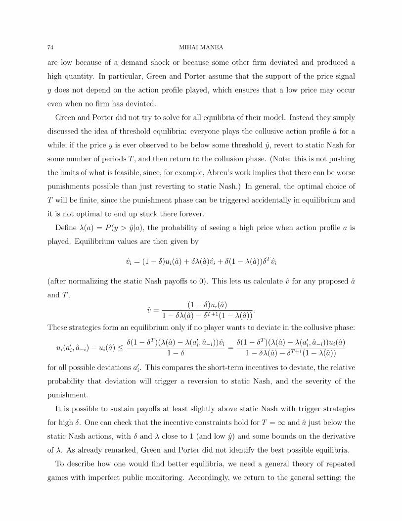
74 MIHAI MANEA
are low because of a demand shock or because some other firm deviated and produced a
high quantity. In particular, Green and Porter assume that the support of the price signal
y does not depend on the action profile played, which ensures that a low price may occur
even when no firm has deviated.
Green and Porter did not try to solve for all equilibria of their model. Instead they simply
discussed the idea of threshold equilibria: everyone plays the collusive action profile a for a
while; if the price y is ever observed to be below some threshold y, revert to static Nash for
some number of periods T , and then return to the collusion phase. (Note: this is not pushing
the limits of what is feasible, since, for example, Abreu’s work implies that there can be worse
punishments possible than just reverting to static Nash.) In general, the optimal choice of
T will be finite, since the punishment phase can be triggered accidentally in equilibrium and
it is not optimal to end up stuck there forever.
Define λ(a) = P (y > y|a), the probability of seeing a high price when action profile a is
played. Equilibrium values are then given by
vi = (1− δ)ui(a) + δλ(a)vi + δ(1− λ(a))δT vi
(after normalizing the static Nash payoffs to 0). This lets us calculate v for any proposed a
and T ,(1 u )
ˆ− δ) i(a
v = .1− δλ(a)− δT+1(1− λ(a))
These strategies form an equilibrium only if no player wants to deviate in the collusive phase:
δ(1− δT )(λ(a)− λ(a′ui(a
′i, a (a)−i)− ui ≤ i, a−i))vi
1− δ=δ(1− δT )(λ(a)− λ(a′i, a−i))ui(a)
1− δλ(a)− δT+1(1− λ(a))
for all possible deviations a′i. This compares the short-term incentives to deviate, the relative
probability that deviation will trigger a reversion to static Nash, and the severity of the
punishment.
It is possible to sustain payoffs at least slightly above static Nash with trigger strategies
for high δ. One can check that the incentive constraints hold for T =∞ and a just below the
static Nash actions, with δ and λ close to 1 (and low y) and some bounds on the derivative
of λ. As already remarked, Green and Porter did not identify the best possible equilibria.
To describe how one would find better equilibria, we need a general theory of repeated
games with imperfect public monitoring. Accordingly, we return to the general setting; the
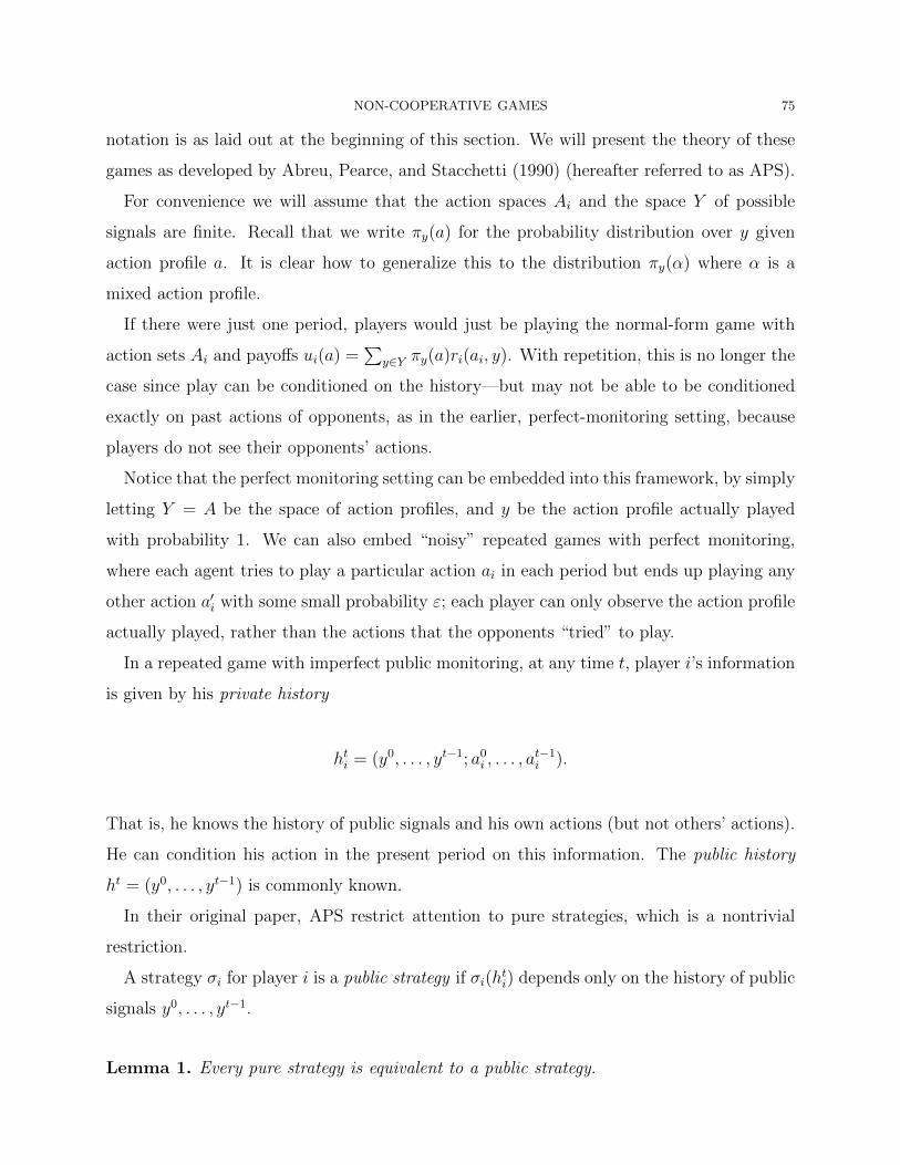
NON-COOPERATIVE GAMES 75
notation is as laid out at the beginning of this section. We will present the theory of these
games as developed by Abreu, Pearce, and Stacchetti (1990) (hereafter referred to as APS).
For convenience we will assume that the action spaces Ai and the space Y of possible
signals are finite. Recall that we write πy(a) for the probability distribution over y given
action profile a. It is clear how to generalize this to the distribution πy(α) where α is a
mixed action profile.
If there were just one period, players would just be playing the normal-form game with
action sets Ai and payoffs ui(a) =∑
y Y πy(a)ri(ai, y). With repetition, this is no longer the∈
case since play can be conditioned on the history—but may not be able to be conditioned
exactly on past actions of opponents, as in the earlier, perfect-monitoring setting, because
players do not see their opponents’ actions.
Notice that the perfect monitoring setting can be embedded into this framework, by simply
letting Y = A be the space of action profiles, and y be the action profile actually played
with probability 1. We can also embed “noisy” repeated games with perfect monitoring,
where each agent tries to play a particular action ai in each period but ends up playing any
other action a′i with some small probability ε; each player can only observe the action profile
actually played, rather than the actions that the opponents “tried” to play.
In a repeated game with imperfect public monitoring, at any time t, player i’s information
is given by his private history
hti = (y0, . . . , yt−1; a0i , . . . , a
ti−1).
That is, he knows the history of public signals and his own actions (but not others’ actions).
He can condition his action in the present period on this information. The public history
ht = (y0, . . . , yt−1) is commonly known.
In their original paper, APS restrict attention to pure strategies, which is a nontrivial
restriction.
A strategy σi for player i is a public strategy if σi(hti) depends only on the history of public
signals y0, . . . , yt−1.
Lemma 1. Every pure strategy is equivalent to a public strategy.
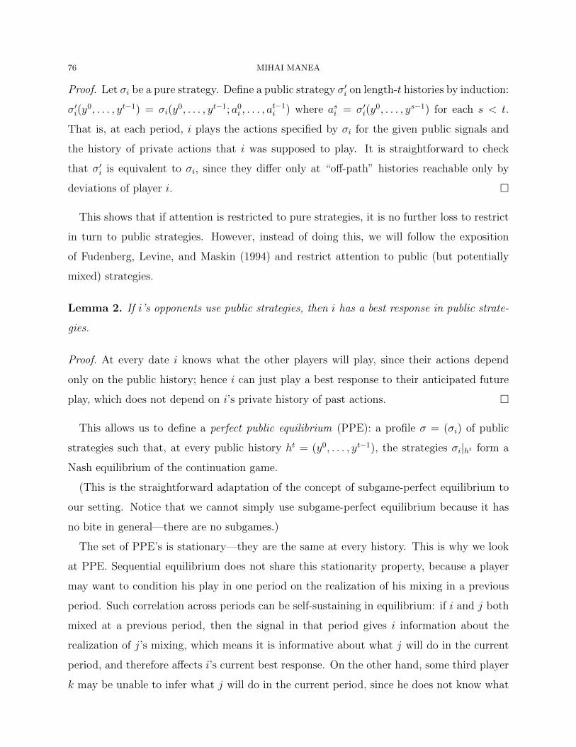
76 MIHAI MANEA
Proof. Let σi be a pure strategy. Define a public strategy σi′ on length-t histories by induction:
σi′(y0, . . . , yt−1) = σi(y
0, . . . , yt−1; a0i , . . . , a
t−1i ) where asi = σ 0
i′(y , . . . , ys−1) for each s < t.
That is, at each period, i plays the actions specified by σi for the given public signals and
the history of private actions that i was supposed to play. It is straightforward to check
that σi′ is equivalent to σi, since they differ only at “off-path” histories reachable only by
deviations of player i.
This shows that if attention is restricted to pure strategies, it is no further loss to restrict
in turn to public strategies. However, instead of doing this, we will follow the exposition
of Fudenberg, Levine, and Maskin (1994) and restrict attention to public (but potentially
mixed) strategies.
Lemma 2. If i’s opponents use public strategies, then i has a best response in public strate-
gies.
Proof. At every date i knows what the other players will play, since their actions depend
only on the public history; hence i can just play a best response to their anticipated future
play, which does not depend on i’s private history of past actions.
This allows us to define a perfect public equilibrium (PPE): a profile σ = (σi) of public
strategies such that, at every public history ht = (y0, . . . , yt−1), the strategies σi|ht form a
Nash equilibrium of the continuation game.
(This is the straightforward adaptation of the concept of subgame-perfect equilibrium to
our setting. Notice that we cannot simply use subgame-perfect equilibrium because it has
no bite in general—there are no subgames.)
The set of PPE’s is stationary—they are the same at every history. This is why we look
at PPE. Sequential equilibrium does not share this stationarity property, because a player
may want to condition his play in one period on the realization of his mixing in a previous
period. Such correlation across periods can be self-sustaining in equilibrium: if i and j both
mixed at a previous period, then the signal in that period gives i information about the
realization of j’s mixing, which means it is informative about what j will do in the current
period, and therefore affects i’s current best response. On the other hand, some third player
k may be unable to infer what j will do in the current period, since he does not know what
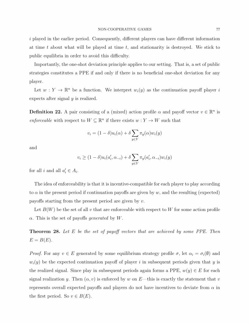
NON-COOPERATIVE GAMES 77
i played in the earlier period. Consequently, different players can have different information
at time t about what will be played at time t, and stationarity is destroyed. We stick to
public equilibria in order to avoid this difficulty.
Importantly, the one-shot deviation principle applies to our setting. That is, a set of public
strategies constitutes a PPE if and only if there is no beneficial one-shot deviation for any
player.
Let w : Y → Rn be a function. We interpret wi(y) as the continuation payoff player i
expects after signal y is realized.
Definition 22. A pair consisting of a (mixed) action profile α and payoff vector v ∈ Rn is
enforceable with respect to W ⊆ Rn if there exists w : Y → W such that
vi = (1− δ)ui(α) + δ∑
πy(α)wi(y)y∈Y
and
vi ≥ (1− δ)ui(a′i, α i) + δ∑
πy(a′i, α i)w (− − i y)
y∈Y
for all i and all a′i ∈ Ai.
The idea of enforceability is that it is incentive-compatible for each player to play according
to α in the present period if continuation payoffs are given by w, and the resulting (expected)
payoffs starting from the present period are given by v.
Let B(W ) be the set of all v that are enforceable with respect to W for some action profile
α. This is the set of payoffs generated by W .
Theorem 28. Let E be the set of payoff vectors that are achieved by some PPE. Then
E = B(E).
Proof. For any v ∈ E generated by some equilibrium strategy profile σ, let αi = σi(∅) and
wi(y) be the expected continuation payoff of player i in subsequent periods given that y is
the realized signal. Since play in subsequent periods again forms a PPE, w(y) ∈ E for each
signal realization y. Then (α, v) is enforced by w on E—this is exactly the statement that v
represents overall expected payoffs and players do not have incentives to deviate from α in
the first period. So v ∈ B(E).
78 MIHAI MANEA
Conversely, if v ∈ B(E), let (α, v) be enforced by w on E. Consider the strategies
defined as follows: play α in the first period, and whatever signal y is observed, play in
subsequent periods follows a PPE with payoffs w(y). These strategies form a PPE, by the
one-shot deviation principle: enforcement means that there is no incentive to deviate in
the first period, and the fact that continuation play is given by a PPE ensures that there
is no incentive to deviate in any subsequent period. Finally it is straightforward from the
definition of enforcement that the payoffs are in fact given by v. Thus v ∈ E.
Definition 23. W ⊆ Rn is self-generating if W ⊆ B(W ).
We have shown that E is self-generating. The next result shows that E is the largest
bounded self-generating set.
Theorem 29. If W is a bounded, self-generating set, then W ⊆ E.
Proof. Let v ∈ W . We want to construct a PPE with payoffs given by v. We construct the
strategies iteratively, simultaneously specifying, for each public history ht = (y0, . . . , yt−1),
the strategies to be played and the continuation values that each player should expect from
subsequent play for each realization of the signal.
The base case, t = 0, has players receiving continuation payoffs given by v. Now suppose
we have specified play for periods 0, . . . , t − 1, and promised continuation payoffs for each
history of signals y0, . . . , yt−1.
Suppose the history of public signals so far is y0, . . . , yt−1 and promised continuation
payoffs are given by v′ ∈ W . Because W is self-generating, there is some action profile α
and some w : Y → W such that (α, v′) is enforced by w. Specify that the players play α at
this history, and whatever signal y is observed, their continuation payoffs starting from the
next period should be w(y).
The expected payoffs following any public history match the target continuation payoffs;
in particular, the constructed strategies generate expected payoffs of v at time 0. This follows
from the adding-up identities, since they ensure that the continuation payoff following any
public history ht equals the expected total payoffs across the following s periods plus δs times
the promised continuation payoff from period t+s onward, and the latter converges to zero as
s→∞. Here the assumption that W is bounded is essential; otherwise we could run a Ponzi
NON-COOPERATIVE GAMES 79
scheme with promised continuation payoffs. Finally, these strategies form a PPE—this is
easily checked using the one-shot deviation principle. Enforcement means exactly that there
are no incentives to deviate at any history.
In addition to obtaining this characterization of the set of PPE payoffs, Abreu, Pearce, and
Stacchetti also prove a monotonicity property with respect to the discount factor. Let E(δ)
be the set of PPE payoffs when the discount factor is δ. Suppose that E(δ) is convex: this
can be achieved either by incorporating public randomization into the model, or by having
a sufficiently rich space of public signals (however, in our version of the model Y is finite).
Then if δ1 < δ2 we have E(δ1) ⊆ B(E(δ1), δ2), and therefore, by the previous theorem,
E(δ1) ⊆ E(δ2). This is shown by the following approach: given v ∈ E(δ1) = B(E(δ1), δ1),
find α and w that enforce v when the discount factor is δ1; then we can enforce (α, v) for
discount factor δ2 with continuation payoffs given by a suitable convex combination of w and
(the constant function) v. The operator B has the following properties.
• If W is compact, so is B(W ). This is shown by a straightforward topological argu-
ment.
• B is monotone: if W ⊆ W ′ then B(W ) ⊆ B(W ′).
• If W is nonempty, so is B(W ). To show this, just let α be a Nash equilibrium of the
stage game, w : Y → W a constant function, and v the resulting payoffs.
Now let V be the set of all feasible payoffs, which is certainly compact. Consider the
sequence of iterates B0(V ), B1(V ), . . ., where B0(V ) = V and Bk(V ) = B(Bk−1(V )). By
induction, these sets are compact and form a decreasing sequence. Hence, their intersection
B∞(V ) is non-empty and compact. Since E ⊆ V and E = B(E), the set E is contained in
each term of the sequence, so E ⊆ B∞(V ).
Theorem 30. E = B∞(V ).
Proof. We are left to prove that B∞(V ) ⊆ E. It suffices to show that B∞(V ) is self-
generating. Suppose v ∈ B∞(V ). Then there exists (αk, wk)k≥1 such that (αk, v) is enforced
by some wk : Y → Bk−1(V ). By compactness, this sequence has a convergent subsequence.
Let (α∞, w∞) denote the limit of such a subsequence. It must be that w∞(y) ∈ B∞(V ) since
w∞(y) is a limit point of the closed set Bk(V ) for all k. By continuity, (α∞, v) is enforced
by w∞ : Y → B∞(V ), so v ∈ B(B∞(V )).
80 MIHAI MANEA
This result characterizes the set of PPE payoffs: if we start with the set of all feasible
payoffs and apply the operator B repeatedly, then the resulting sequence of sets converges
to the set of equilibrium payoffs.
Corollary 4. The set of PPE payoff vectors is nonempty and compact.
(Nonemptiness is immediate because, for example, the infinite repetition of any static NE
is a PPE.)
In their setting with finite action spaces and continuous signals with a common support,
APS also show a “bang-bang” property of perfect public equilibria. We say that w : Y → W
has the bang-bang property if w(y) is an extreme point of W for each y. They show that if
(α, v) is enforceable on a compact W , it is in fact enforceable on the set ext(W ) of extreme
points of W . Consequently, every vector in E can be achieved as the vector of payoffs from
a PPE such that the vector of continuation payoffs at every history lies in ext(E).
28. The Folk Theorem for Imperfect Public Monitoring
Fudenberg, Levine, and Maskin (1994) (hereafter FLM) prove a folk theorem for repeated
games with imperfect public monitoring. They identify conditions on the stage game—
particularly on how informative public signals need to be about actions—under which it
is possible to construct convex sets with a smoothly curved boundary, approximating the
set of feasible, individually rational payoffs arbitrarily closely that are self-generating for
sufficiently high discount factors. This implies that a folk theorem obtains.
The proof is fairly complicated. We will briefly discuss the technical difficulties involved.
First, there has to be statistical identifiability of each player’s actions. If player i’s deviation
to αi′ generates exactly the same distribution over signals as some mixed action αi he is
supposed to play (given opponents’ play α i), but gives him a higher payoff on average, then−
clearly there is no way to enforce the action profile α in equilibrium. To avoid this problem,
FLM assume an individual full-rank condition: given α ,−i the different signal distributions
generated by varying i’s pure actions ai are linearly independent.
They need to further assume a pairwise full rank condition: deviations by player i are
statistically distinguishable from deviations by player j. Intuitively this is necessary because,
if the signal suggests that someone has deviated, the players need to know who to punish.
NON-COOPERATIVE GAMES 81
(Radner, Myerson, and Maskin (1986) give an example of a game that violates this condition
and where the folk theorem does not hold. There are two workers who put in effort to increase
the probability that a project succeeds; they both get 1 if it succeeds and 0 otherwise. The
outcome of the project does not statistically distinguish between shirking by player 1 and
shirking by player 2. So if the project fails, both players have to be punished by giving them
lower continuation payoffs than if it succeeds. Because it fails some of the time even if both
players are working, this means that equilibrium payoffs are bounded away from efficiency,
even as δ → 1.)
The statement of the pairwise full rank condition is as follows: given the action profile α,
if we form one matrix whose rows represent the signal distributions from (ai, α i) as ai varies−
over Ai, and another matrix whose rows represent the signal distributions from (aj, α−j) as
aj varies over Aj, and stack these two matrices, the combined matrix has rank |Ai|+ |Aj|−1.
(This is effectively “full rank”—it is not possible to have literal full rank |Ai| + |Aj|, since
the signal distribution generated by α is a linear combination of the rows of the first matrix
and is also a linear combination of the rows of the second matrix.)
When this condition is satisfied, it is possible to use continuation payoffs to transfer utility
between the two players i, j in any desired ratio, depending on the signal, so as to incentivize
i and j to play according to the desired action profile.
Having imposed appropriate formulations of these conditions, FLM show that the W they
construct is locally self-generating : for every v ∈ W , there is an open neighborhood U and
a δ < 1 such that U ∩W ⊆ B(W ) when δ > δ. This definition allows δ to vary with v. For
W compact and convex, they show that local self-generation implies self-generation for all
sufficiently high δ.
The intuition behind their approach to proving local self-generation is best grasped with
a picture. Suppose we want to achieve some payoff vector v on the boundary of W . The
full-rank conditions ensure we can enforce it using some continuation payoffs that lie below
the tangent hyperplane to W at v, by “transferring” continuation utility between players as
described above. As δ → 1, the continuation payoffs sufficient to enforce v contract toward
v, and the smoothness condition on the boundary of W ensures that they will eventually lie
inside W . Thus (α, v) is enforced on W .
[PICTURE—See p. 1013 of Fudenberg, Levine, Maskin (1994)]
82 MIHAI MANEA
Some extra work is needed to take care of the points v where the tangent hyperplane is a
coordinate hyperplane (i.e. one player’s payoff is constant on this hyperplane).
An argument along these lines shows that every vector on the boundary of W is achievable
using continuation payoffs in W , when δ is high enough. Using public randomization among
boundary points, we can then achieve any payoff vector v in the interior of W as well. It
follows that W is self-generating (for high δ).
29. Changing the Information Structure with Time Period
Follow FT pp. 197-200. Suppose players have a discount rate r and can only update
their actions at times t, 2t, . . .. Then the effective discount rate is δ = e−rt. Hence the
limit δ → 1 has two interpretations: either players become patient (r → 0) or periods are
short (t → 0). In games where actions are observable, as well as games with imperfect
public monitoring in which the amount of information revealed does not change with t, the
variables r and t enter symmetrically in δ and the limit set of PPE payoffs as δ → 1 can
be interpreted both as the outcome when players are patient and when periods are short.
However, if monitoring is imperfect and the quality of signals deteriorates as t→ 0, then the
short period interpretation is lost.
Abreu, Milgrom, and Pearce (1991) point out that the two limits r → 0 and t → 0 may
lead to distinct predictions. They focus on partnership games where the expected payoffs in
the stage game induce the structure of prisoners’ dilemma. Players do not directly observe
each other’s level of effort. Instead, the total level of effort is imperfectly reflected in a public
signal, interpreted as the number of “successes.” The signal has a Poisson distribution with
an intensity parameter λ if both players cooperate and µ if one of them defects. Assume
that λ > µ, so that signals indeed represent “good news.”18 For small t, the probability
of observing more than one success is of order t2. As in FT, we simplify the analysis by
approximating the signal structure with a setting in which there are either 0 or 1 successes
observed, with probabilities e−θt and 1− e−θt, respectively, for θ ∈ λ, µ.
Let c denote the common payoff when both players cooperate, and c + g the payoff a
player obtains from defecting when the other cooperates; payoffs when both players defect
are normalized to 0. The static Nash equilibrium (defect, defect) generates the minmax
18AMP also analyze the case of “bad news,” where signals indicate failures.
NON-COOPERATIVE GAMES 83
payoff for both players. Hence the worst equilibrium for either player in the repeated game
delivers zero payoffs.
Restrict attention to pure strategy strongly symmetric equilibria. Let v∗ denote the payoff
in an optimal equilibrium within this class. It can be easily seen that such an equilibrium
must specify cooperation in the first period. Suppose that a public randomization device
is available, so that continuation play when the number of successes observed is i = 0, 1
can be described by playing the worst equilibrium (minmax, static Nash), with 0 payoffs,
with probability α(i) and the best equilibrium, which yields common continuation payoffs
v∗, with probability 1− α(i).
The relevant PPE constraints are
v∗ = (1− e−rt)c+ e−rt(e−λt(1− α(0)) + (1− e−λt)(1− α(1)) v∗
≥ (1− e−rt)(c+ g) + e−rt(e−µt(1− α(0)) + (1
)− e−µt)(1− α(1)) v∗
Solving for v∗ in the first equation, we obtain
)
(1 cv∗
− e−rt)= .
1− e−rt (1− α(1)− e−λt(α(0)− α(1)))
The incentive constraint becomes
(1− e−rt)g ≤ e−rt(e−µt − e−λt)(α(0)− α(1))v∗,
which simplifies toce−rt(e−µt
g− e−λt)(α(0)− α(1))≤ .
1− e−rt (1− α(1)− e−λt(α(0)− α(1)))
Note that v∗ is decreasing in α(1) and the incentive constraint is also relaxed by decreas-
ing α(1). Hence an optimal symmetric equilibrium in pure strategies specifies α(1) = 0.
Intuitively, an optimal equilibrium should not involve any punishment if a success occurs.
Setting α(1) = 0, the constraints become
(1v∗ =
− e−rt)c1− e−rt(1− e−λtα(0))
e−rt(e−µtg/c
− e−λt)α(0)≤1− e−rt(1− e−λtα(0))
It is possible to satisfy the inequality for α(0) ≤ 1 only if
e−rt(e−µt(29.1) g/c
− e−λt)≤1− e−rt(1− e−λt)
84 MIHAI MANEA
Note thate−rt(e−µt − e−λt) ≤ e(λ−µ)t
1− e−rt(1− e−λt)− 1.
The RHS of the inequality above converges to 0 as t→ 0. Hence an equilibrium with payoffs
above static Nash does not exist for small t. The term e(λ−µ)t can be interpreted as the
likelihood ratio for no success. As t → 0 this ratio converges to 1. Since we are almost
certain that no success occurs even when both players exert effort, the information provided
by the public signal is too poor for there to be an equilibrium that improves on the static
Nash outcome.
Taking the limit r → 0 in ??, we obtain
(29.2) g/c ≤ e(λ−µ)t − 1.
Hence an equilibrium with the desired properties exists for small r and certain values of t.
For the “optimal” (minimum) α(0), we find that when ?? holds,
glim v∗ = cr→0
− ,e(λ−µ)t − 1
which is greater than limt 0 v∗ = 0 when ?? is satisfied with strict inequality.→
30. Reputation
Repeated games provide a useful setting for studying the concept of reputation build-
ing. The earliest repeated-game models of reputation were by the Gang of Four (Kreps,
Milgrom, Roberts, and Wilson); in various combinations they wrote three papers that were
simultaneously published in JET 1982.
The motivating example was the “chain-store paradox.” In the chain-store game, there
are two players, an entering firm and an incumbent monopolist. The entrant (player 1) can
enter or stay out; if it enters, the incumbent (player 2) can fight or not. If the entrant stays
out, payoffs are (0, a) where a > 1. If the entrant enters and the incumbent does not fight,
the payoffs are (b, 0) where b ∈ (0, 1). If they do fight, payoffs are (b − 1,−1). There is a
unique SPE, in which the entrant enters and the incumbent does not fight.
In reality, incumbent firms seem to fight when a rival enters, and thereby deter other
potential rivals. Why would they do this? In a one-shot game, it is irrational for the
incumbent to fight the entrant. As pointed out by Selten, even if the game is repeated finitely
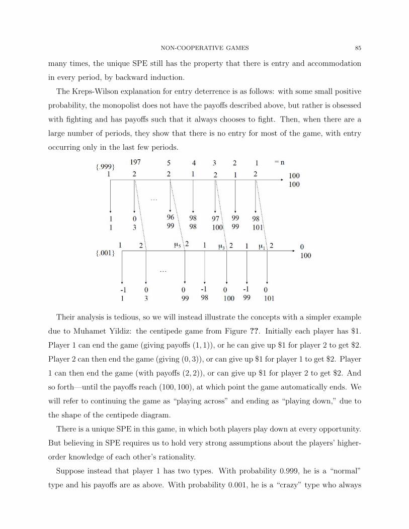
NON-COOPERATIVE GAMES 85
many times, the unique SPE still has the property that there is entry and accommodation
in every period, by backward induction.
The Kreps-Wilson explanation for entry deterrence is as follows: with some small positive
probability, the monopolist does not have the payoffs described above, but rather is obsessed
with fighting and has payoffs such that it always chooses to fight. Then, when there are a
large number of periods, they show that there is no entry for most of the game, with entry
occurring only in the last few periods.
Their analysis is tedious, so we will instead illustrate the concepts with a simpler example
due to Muhamet Yildiz: the centipede game from Figure ??. Initially each player has $1.
Player 1 can end the game (giving payoffs (1, 1)), or he can give up $1 for player 2 to get $2.
Player 2 can then end the game (giving (0, 3)), or can give up $1 for player 1 to get $2. Player
1 can then end the game (with payoffs (2, 2)), or can give up $1 for player 2 to get $2. And
so forth—until the payoffs reach (100, 100), at which point the game automatically ends. We
will refer to continuing the game as “playing across” and ending as “playing down,” due to
the shape of the centipede diagram.
There is a unique SPE in this game, in which both players play down at every opportunity.
But believing in SPE requires us to hold very strong assumptions about the players’ higher-
order knowledge of each other’s rationality.
Suppose instead that player 1 has two types. With probability 0.999, he is a “normal”
type and his payoffs are as above. With probability 0.001, he is a “crazy” type who always
86 MIHAI MANEA
gets utility −1 if he ends the game and 0 if player 2 ends the game. (Player 2’s payoffs are
the same regardless of 1’s type.) The crazy type of player 1 thus always wants to continue
the game. Player 2 never observes player 1’s type.
What happens in equilibrium? Initially player 1 has a low probability of being the crazy
type. If the normal player 1 plays down at some information set, and the crazy player 1
across, then after 1 plays across, player 2 must infer that 1 is crazy. But if player 1 is crazy
then he will continue the game until the end; knowing this, player 2 also wants to play across
in order to accumulate money. Anticipating this, the normal type of player 1 in turn also
wants to play across in order to get a high payoff.
With this intuition laid out, we analyze the game formally and describe the sequential
equilibria. Number the periods, starting from the end, with 1 being player 2’s last information
set, 2 being player 1’s previous information set,. . ., 198 being 1’s first information set. The
crazy player 1 always plays across.
Player 2 always plays across with positive probability at every period n > 1. (Proof: if
not, then the normal player 1 must play down at period n+1. Then, conditional on reaching
n, player 2 knows that 1 is crazy with probability 1, hence he would rather go across and
continue the game to the end.)
Hence there is positive probability of going across at every period, so the beliefs are
uniquely determined from the equilibrium strategies by Bayes’ rule.
Next we see that the normal player 1 plays across with positive probability at every n > 2.
Proof: if not, then again, at n−1 player 2 is sure that he is facing a crazy type and therefore
wants to go across. Given this strategy by player 2, then, the normal 1 also has incentives
to go across at n so that he can go down at n− 2, contradicting the assumption that 1 only
goes down at n.
Next, if 2 goes across with probability 1 at n, then 1 goes across with probability 1 at
n + 1, and this in turn implies that 2 goes across with probability 1 at n + 2. This is also
seen by the same argument as in the previous paragraph. Therefore there is some cutoff
n∗ ≥ 3 such that both players play across with probability 1 at n > n∗, and there is mixing
for 2 < n ≤ n∗. (We know that both the normal 1 and 2 play down with probability 1 at
n = 1, 2.)
NON-COOPERATIVE GAMES 87
Let pn be the probability of the normal type of player 1 going down at n, if n is even. Let
µn be the probability player 2 assigns to the crazy type at node n.
At each odd node n, 2 < n ≤ n∗, player 2 is to be indifferent between going across and
down. The payoff to going down is some x. The payoff to going across is (1− µn)pn (x−1 −
1) + [1 − (1 − µn)pn 1](x + 1), using the fact that player 2 is again indifferent (or strictly−
prefers going down) two nodes later. Hence we get (1 − µn)pn−1 = 1/2: player 2 expects
player 1 to play down with probability 1/2. But µn−2 = µn/(µn + (1 − µn)(1 − pn−1)) by
Bayes’ rule; this simplifies to µn−2 = µn/(1 − (1 − µn)pn 1) = 2µn. We already know that−
µ1 = 1 since the normal player 1 goes down with certainty at node 2. Therefore µ3 = 1/2,
µ5 = 1/4, and so forth; and in particular n∗ ≤ 20, since otherwise µ21 = 1/1024 < 0.001,
but clearly the posterior probability of the crazy type at any node cannot be lower than the
prior. This shows that for all but the last 20 periods, both players are going across with
probability 1 in equilibrium.
(One can in fact continue to solve for the complete description of the sequential equilib-
rium: now that we know player 2’s posterior at each period, we can compute player 1’s mixing
probabilities from Bayes’ rule, and we can also compute player 2’s mixing probabilities given
that 1 must be indifferent whenever he mixes.)
This model illustrates the way that the concept of reputation is generally modeled in
repeated games. A player develops a reputation for playing a certain action; in equilibrium
it is rational for him to continue with that action in order to maintain the reputation, even
though it would not be rational in a one-shot setting. Unraveling is prevented by having a
small probability of a type that is committed to that action.
The papers by the Gang of Four consider repeated interactions between the same players,
with one-sided incomplete information. Inspired by this work, Fudenberg and Levine (1989)
consider a model in which a long-run player faces a series of short-run players, and where there
are many possible “crazy” types of the long-run player, each with small positive probability.
They show that if the long-run player is sufficiently patient, he will get close to his Stackelberg
payoff in any Nash equilibrium of the repeated game.
The model is as follows. There are two players, playing the finite normal-form game
(N,A, u) (with N = 1, 2) in each period. Player 1 is a long-run player. Player 2 is a
short-run player (which we can think of as a series of players who play for one period each,

88 MIHAI MANEA
or one very impatient player). Incentive for short-run players are simple: they best respond
to the long-run player’s anticipated action in each stage.
Define
u∗1 = max min u1(a1, σ2).a1∈A1 σ2∈BR2(a1)
This is player 1’s Stackelberg payoff ; the action a∗1 that achieves this maximum is the Stack-
elberg action. Fudenberg and Levine (1989) only considers pure action selections by player
1. The analysis is extended to mixed actions in a follow-up paper published in 1992.
A strategy for player 1 consists of a function σt1 : H t−1 → ∆(A1) for each t ≥ 0. A strategy
for the player 2 who plays at time t consists of a function σt : H t−12 → ∆(A2). With the
usual discounted payoff formulation, the game described constitutes the unperturbed game.
Fudenberg, Kreps, and Maskin (1988) prove a version of the folk theorem for this game.
Let B2 denote the set of mixed strategy best responses in the stage game for the short run
players to mixed strategies of the long run player. Set
u1 = minσ2∈B2
maxa1∈A1
u1(a1, σ2).
Fudenberg, Kreps, and Maskin show that any payoff above u1 can be sustained in SPE for
high enough δ. The main reputation result of Fudenberg and Levine shows that if there is
a rich space of crazy types of player 1, each with positive probability, this folk theorem is
completely overturned—player 1 obtains a payoff of at least u∗1 in any Nash (not necessarily
subgame perfect) equilibrium for high δ. Note that for the standard Cournot duopoly with
two firms and linear demand, u1 and u∗1 correspond to the follower and leader payoffs,
respectively.
Accordingly, we consider the perturbed game, where there is a countable state space Ω.
Player 1’s payoff depends on the state ω ∈ Ω; thus write u1(a1, a2, ω). Player 2’s payoff does
not depend on ω. There is some prior distribution µ on Ω, and the true state is known only
to player 1. When the state is ω0 ∈ Ω, player 1’s payoffs are given by the original u1; we call
this the “rational” type of player 1.
Suppose that for every a1 ∈ A1, there is a state ω(a1) for which playing a1 at every
history is a strictly dominant strategy in the repeated game.19 Thus, at state ω(a1), player
19Assuming it is strictly dominant in the stage game is not enough. For instance, defection is a dominantstrategy in prisoners’ dilemma, but always defecting is not a best response agains tit-for-tat in the repeatedgame.
NON-COOPERATIVE GAMES 89
1 is guaranteed to play a1 at every history. Write ω∗ = ω(a∗1). We assume also that
µ∗ = µ(ω∗) > 0. That is, with positive probability, player 1 is a type who is guaranteed to
play a∗1 in every period.
Any strategy profile generates a joint probability distribution π over play paths and states,
π ∈ ∆((A1×A2)∞×Ω). Let h∗ be the event (in this path-state space) that at1 = a∗1 for all t.
Let πt∗ = π(at1 = a∗1|ht−1), the probability of seeing a∗1 at period t given the previous history;
this is a random variable (defined on path-state space) whose value is a function of ht−1. For
any number π ∈ (0, 1), let n(π∗t ≤ π) denote the number of periods t such that π∗t ≤ π. This
is again a random variable, whose value may be infinite.
The next result provides the main ingredient of the analysis. Conditional on observing
a∗1 every period, it is guaranteed that there are at most lnµ∗/ lnπ periods in which a∗1 is
expected with probability below π conditional on the history. In other words, player 2 can
be surprised by seeing a∗1 only a finite number of times.
Lemma 3. Let σ be a strategy profile such that π(h∗|ω∗) = 1. Then
π
(n(πt
∗ ≤ π) ≤ lnµ∗
ln1
π
∣∣h∗)
= .
Given that π(h∗|ω∗) = 1, if the true state is ω∗, then
∣∣player 1 will always play a∗1. Every
time the probability of seeing a∗1 next period is less than π, if a∗1 is in fact played, the posterior
probability of ω∗ must increase by a factor of at least 1/π. The posterior probability starts
out at µ∗ and can never exceed 1, so it can increase no more than lnµ∗/ lnπ times.
Formally, consider any finite history ht at which a∗1 has been played every period, and such
that π(ht) > 0. Write ht,1 (ht,2) for the event where ht−1 is observed and then at period t
player 1 (2) plays as in ht. We have that
π(ω∗|ht π(ht & ω∗ ))
|ht−1
=π(ht|ht−1)
=π(ω∗|ht−1)π(ht|ω∗, ht−1)
π(ht|ht−1)
π(ω∗|ht−1)π(ht,1=
|ω∗, ht−1)π(ht,2|ω∗, ht−1)
π(ht,1|ht−1)π(ht,2|ht−1)
π(ω∗=
|ht−1)π(ht,2|ω∗, ht−1)
π(ht,1|ht−1)π(ht,2
t 1
|ht−1)
π(ω∗=
|h − )
π∗t.
90 MIHAI MANEA
Here the first line of equalities uses Bayes’ rule, the second holds because 1 and 2 mix
independently at period t, the third holds because if ω∗ occurs then at1 = a∗1, and the fourth
holds because player 2’s behavior conditional on the history ht−1 cannot depend on 1’s type.
Repeatedly expanding, we have
)π(ω∗| t π(ω∗
) =|ht−1
hπ∗t
= . . . =π(ω∗|h0)
π∗t π∗t−1 · · · π∗0
=µ∗
π∗t π∗t−1 · · · π∗0
.
Since π(ω∗|ht) ≤ 1, at most lnµ∗/ lnπ terms in the denominator of the last expression can
be less than or equal to π. Therefore, n(π∗t ≤ π) ≤ lnµ∗/ lnπ with probability 1.
Now we get to the main theorem. Let um = minσ2 u1(a∗1, σ2, ω0) denote the worst possible
stage payoff for player 1 when he takes action a∗1. Note that the payoff u∗1 is a “lower
Stackelberg payoff.” There is also an “upper Stackelberg payoff” in the stage game,
u1 = max max u1(a1, a2).a1 σ2∈BR2(a1)
Let uM = maxa u1(a, ω0) denote the highest payoff for the rational type of player 1 in the
stage game. Denote by v1(δ, µ, ω0) and v1(δ, µ, ω0) the infimum and supremum, respectively,
of rational player 1’s payoffs in the repeated game across all Nash equilibria in which player
1 uses a pure strategy, for given discount factor δ and prior µ.
Theorem 31. For any value µ∗, there exists a number κ(µ∗) with the following property:
for all δ and all (µ,Ω) with µ(ω∗) = µ∗, we have
v κ1(δ, µ, ω0) ≥ δ (µ∗)u∗1 + (1− δκ(µ∗))um.
Moreover, there exists κ such that for all δ, we have
v1(δ, µ, ω0) ≤ δκu1 + (1− δκ)uM .
As δ → 1, the payoff bounds converge to u∗1 and u1, which are generically identical.
Proof. First, note that there exists a π < 1 such that, in every play path of every Nash
equilibrium, at every stage t where π∗t > π, player 2 plays a best response to a∗1. This follows
from the fact that the pure strategy best response correspondence has a closed graph and
the assumption that action spaces are finite.
Thus, by the lemma, we have a number κ(µ∗) of periods such that π(n(π∗ ≤ π) >
κ(µ∗) | h∗) = 0. Now, whatever player 2’s equilibrium strategy is, if the rational player
NON-COOPERATIVE GAMES 91
1 deviates to simply playing a∗1 every period, there are at most κ(µ∗) periods in which player
2 will not play a best response to a∗1—since player 2 is playing a best response to player 1’s
expected play in each period. Thus the rational player 1 gets a stage payoff of at least um
in each of these periods, and least u∗1 in all the other periods. This immediately gives that
player 1’s payoff from deviating is at least δκ(µ∗)u∗1 + (1 − δκ(µ∗))um. Since we have a Nash
equilibrium, player 1’s payoff in equilibrium is at least his payoff from deviating.
An argument similar to the one above establishes the second bound. The idea is to obtain
a version of Lemma ?? with ω∗ replaced by ω0. Players may be surprised by the behavior of
type ω0 only a finite number of times. In all other periods, they must play a best response
to the expected play of ω0.
Fudenberg and Levine (1992) extend the result to mixed strategy Nash equilibria. In
generic games, the lower and upper Stackelberg payoffs coincide and we get a unique equi-
librium payoff for the rational player 1 in the limit as δ → 1.
31. Reputation and Bargaining
Abreu and Gul (2000) consider reputation in the context of bargaining. Two players need
to divide $1. Every player can be either rational or a crazy type who always demands a fixed
share of the dollar. Each player wants to develop a reputation for being irrational in order
to get his opponent to concede to his demand.
The bargaining protocol is very general. Every player is allowed to make offers at a discrete
set of dates. The analysis focuses on the continuous time limit in which each player gets
the opportunity to make offers in every time interval. It turns out that the details of the
bargaining protocol do not affect the limit outcomes.
Abreu and Gul show that whenever either player i has revealed himself to be rational
by doing anything other than demanding αi, there will be almost immediate agreement: j
can get himself a share close to αj by continuing to use his reputation, leading i to concede
quickly in equilibrium. This is similar to the Fudenberg-Levine reputation result, but it
turns out to be complicated to prove. So what happens in equilibrium if both players are
rational? They play a war of attrition—each player pretends to be irrational but has some
probability of conceding at each period (by revealing rationality), and as soon as one concedes
the ensuing payoffs are those given by the reputation story. These concession probabilities
92 MIHAI MANEA
must make each player indifferent between conceding and not; from this we can show that
the probabilities are stationary, up to some finite time, and if both players have not conceded
by that time they must be irrational (and so will never concede).
The setting is as follows. There are two players i = 1, 2. Player i has discount rate ri.
If an agreement (x1, x2) is reached at time t, the payoffs (if the players are rational) are
(x e−r1t1 , x2e−r2t). Each player i, in additional to his rational type, has an irrational type,
whose behavior is fixed: this type always demands αi, and always accepts offers that give
him at least αi and rejects lower offers. We assume α1 + α2 > 1. The prior probability that
player i is irrational is zi.
We consider bargaining protocols that are a generalization of the Rubinstein alternating-
offers protocol. A protocol is given by a function g : [0,∞) → 0, 1, 2, 3. If g(t) = 0, then
nothing happens at time t. If g(t) = 1 then player 1 makes an offer, and 2 immediately
decides whether to accept or reject. If g(t) = 2 then the same happens with players 1 and 2
reversed. If g(t) = 3 then both players simultaneously offer. If their offers are incompatible
(the amount player 1 demands plus the amount player 2 demands exceeds 1) then both offers
are rejected and the game continues; otherwise each player gets what he demands and the
remaining surplus is split equally.
The protocol is discrete, meaning that for every t, g−1(1, 2, 3)∩[0, t) is finite. A sequence
of such protocols (gn) converges to the continuous limit if, for all ε > 0, there exists n∗ such
that for all n > n∗, and for all t, 1, 2 ⊆ gn([t, t + ε]). For example, this is satisfied if
gn is the Rubinstein alternating protocol with time increments of 1/n between offers. As
Abreu and Gul show, each gn induces a game with a unique equilibrium outcome, and these
equilibria converge to the unique equilibrium outcome of the continuous-time limit game.
The continuous-time limit game is a war of attrition. Each player initially demands αi. At
any time, each player can concede or not. Thus, rational player i’s strategy is a probability
distribution over times t ∈ [0,∞] at which to concede (given that j has not already conceded);
t = ∞ corresponds to never conceding. If player i concedes at time t, the payoffs are
(1− αj)e−rit for i and αje−rjt for j. With probability zi, player i is the irrational type who
never concedes. (If there is no concession, both players get payoff 0.)
NON-COOPERATIVE GAMES 93
Bargaining follows a Coasian dynamics once one of the players is revealed to be rational.
The Coase conjecture asserts that when the time between offers is sufficiently small, bar-
gaining between a seller with known valuation v and a buyer who may have one of many
reservation values, all greater than v, results in almost immediate agreement at the lowest
buyer valuation. Myerson’s (1991) text (pp. 399-404) offers a different perspective on this
result by recasting it in a reputational setting. The low valuation buyer is replaced by an
irrational type who demands some constant amount and accepts no less than this amount. In
an alternating offer bargaining game, he shows that as the time between offers goes to zero,
agreement is reached without delay at the constant share demanded by the irrational type.
Similarly, in the Coase conjecture there is immediate agreement at the lowest buyer valua-
tion. Both results are independent of the ex ante probability of the low type and the players’
relative discount factors so long as they are both close to 1, as implied by the assumption
that offers are frequent. Thus, Myerson observes that the influence of asymmetric informa-
tion overwhelms the effect of impatience in determining the division of surplus. Abreu and
Gul extend Myerson’s result as follows.
Lemma 4. For any ε > 0, if n is sufficiently high, then after any history in gn where i has
revealed rationality and j has not, in equilibrium play of the continuation game, i obtains at
most 1− αj + ε and j obtains at least αj − ε.
Proof. Consider the equilibrium continuation play starting from some history at which i has
revealed rationality and j has not as of time t. It is sufficient to show that player j’s payoff
if he continues to act irrationally converges to αj as n → ∞. Let t be any time increment
such that, with positive probability (in this continuation), the game still has not ended at
time t+ t. We will first show that there is an upper bound on t.
Let π be the probability that j does not reveal rationality under the equilibrium strategies
in the interval [t, t + t). Then i’s expected continuation payoff as of time t satisfies vi ≤
1− π + πe−r ˆit. We also have vi ≥ (1− αj)ztj where ztj is the posterior that j is irrational as
of time t, since i could get this much by immediately conceding. Then
1− π + πe−rˆit ≥ (1− α t
j)zj ≥ (1− αj)zj.
It must be that π is bounded above by some π < 1 for large enough t.
94 MIHAI MANEA
Now we apply the reasoning from Fudenberg and Levine (1989). Assume t is large enough
that j always has a chance to offer in any interval of length t. Each time an interval of
length t goes by without j conceding, the posterior probability that j is irrational increases
by a factor of at least 1/π > 1. The number of such increases that can occur is bounded
above (by ln(zi)/ ln(π)). Thus there is an upper bound on the amount of time the game can
continue, as claimed.
The argument above shows that for every n, if player j continues to behave irrationally,
player i concedes in finite time t(n). This time depends on n since we chose t such that j has
an opportunity to make an offer. We next show that t(n) converges to zero as n increases.
Consider the last ε units of time before player i would concede with certainty if j sticks to
his demand. Without loss of generality, assume rj = 1 and ri = r. Since with probability at
least zj player j is irrational, with positive probability player i is using some strategy that
does not end the game for at least ε longer. Fix β ∈ (0, 1). The expected payoff from such
strategy is at most
(1− ζ)x+ ζy
where
• x is i’s expected payoff if j agrees to an offer worse than αj by time βε;
• y is i’s payoff if j does not agree to such an offer by time βε;
• ζ is the probability i assigns to the latter event.
For i to have incentives to wait out ε more time rather than accept the offer αj, it must
be that
(31.1) 1− αj ≤ (1− ζ)x+ ζy.
If j agrees to a payoff less than αj, then i will find out he is rational. But then j knows that
if he holds out for ε longer, he will get αj and, hence, j’s payoff is at least e−εαj. Therefore
x ≤ 1 − e−εαj. Similarly, if j does not agree to an offer by βε, then the best that i can do
after that time is 1− e−(1−β)εαj. So y ≤ e−βrε(1− e−(1−β)εαj). Note that y < 1− αj reduces
to
1 ε
j <− e−βr
α1− e−(βr+1−β)ε
.
NON-COOPERATIVE GAMES 95
In the limit ε→ 0 the latter inequality becomes αj < βr/(βr+ 1− β), which is satisfied for
β > αj/(αj + r(1− αj).
Plugging our bounds into inequality (??) we get
1− αj ≤ 1− e−εαj + ζ(e−βrε(1− e−(1−β)εαj)− (1− e−εαj)).
Note that for small ε, we have e−βrε(1 − e−(1−β)εαj) < 1 − αj < 1 − e−εαj, and hence the
coefficient of ζ above is negative. Reorganizing the terms to get a bound for ζ and taking
the limit ε→ 0 we obtain that
α(31.2) ζ ≤ j
β(αj + (1− αj)r)+ k(ε)
where limε→0 k(ε) = 0.
Fix β ∈(
αj , 1 and let ε > 0 be small enough so that the right-hand side of theαj+(1−αj)r
inequality (??) is strictly
)less than some δ < 1 whenever ε < ε.
Suppose we have a history at time t where i has revealed rationality, j has not, and the
latest possible end of the game (if j continues not conceding) is t + ε. If j does not reveal
rationality by time t + βε, the posterior probability that j is irrational must increase by at
least a factor 1/δ > 1. If j does not reveal rationality by the time (1− β)2ε before the end
of the game, the posterior probability of irrationality must increase by another factor of 1/δ,
and so forth. There can only be some number k of such increments before the posterior
belief exceeds 1. Note that our argument for i’s incentives assumes that i is able to make
offers sufficiently close to each of the cutoffs in the argument above.
As n → ∞, because the offers in the games gn become increasingly frequent, the corre-
sponding upper bounds on ε go to 0. Thus, once i has revealed rationality, the maximum
amount of time that it can take before the game ends if j continues to act irrationally goes
to 0 as n → ∞. This means that by acting irrationally, j can guarantee himself a payoff
arbitrarily close to αj for n sufficiently high.
This leads (with a little further technical work) to the result that the continuous-game
equilibrium is the limit of the discrete-game equilibria. When one agent is known to be
rational and there is a positive probability that her opponent is irrational, delay is not
possible. This means that either the player i known to be rational gives in to the irrational
demand of the other player j or player j also reveals himself to be rational. The latter

96 MIHAI MANEA
outcome occurs only when j receives a payoff no less than αj when he reveals himself to be
rational. Otherwise, j prefers to pretend to be irrational and be conceded to by i without
delay.
With this conclusion in place, a war of attrition emerges: at any time t, player i can
continue pretending to be irrational and wait for j to make the offer 1 − αj or some offer
that reveals j’s rationality. In either situation, i obtains a payoff no less than 1 − αj since
αi > 1 − αj by assumption and i obtains a payoff of at least αi once j reveals himself to
be rational. Thus, player i’s equilibrium payoff before either player reveals rationality is at
least 1 − αj. Whenever j decides to reveal his rationality, i receives a payoff of at least αi,
which means that in equilibrium i and j get exactly αi and 1− αi, respectively. But this is
precisely the set-up of a war of attrition where i’s winning payoff is αi and her losing payoff
is 1− αj.
It remains to analyze the continuous-time war of attrition. This is a well-known game,
but with the twist that there are irrational types. In equilibrium, let Fi denote the cdf of
times when i concedes—unconditional on i’s type; thus limt F→∞ i(t) ≤ 1 − zi because the
irrational player never concedes.
What are the rational player i’s payoffs from holding out until time t, then conceding?
We get
uit = αi
∫ t− 1e−riy dFj(y) +
0
(αi + 1 α )( rij Fj(t) F t
j(t−)) + (1 αj)(1 Fj(t))e
−2
− − − −
(these terms correspond to i winning, both players conceding at the same time, and j winning,
respectively). Assuming that F1 and F2 have a common support and are continuous, it
must be that each uit is constant and differentiable over the support. Taking derivatives
with respect to t we obtain that dFj/(1 − Fj) = ri(1 − αj)/(α1 + α2 − 1) := λj. The
concession rate of player j makes the rational type of player i indifferent about conceding
ˆ ˆeverywhere on his support. Let (F1, F2) be the unique strategy profile satisfying T 0 =
− − ˆmin ( log z1)/λ1, ( log z2)/λ2 , ci = zieλ 0iT , and F (t) = 1 − c e−λiti i . The next result
proves that these functions characterize the unique equilibrium. The proof resembles the
argument showing equilibrium uniqueness in the first-price auction.
ˆ ˆProposition 5. The unique sequential equilibrium is (F1, F2).
NON-COOPERATIVE GAMES 97
Proof. Let σ = (F1, F2) define a sequential equilibrium. We will argue that σ must have the
form specified (i.e., uniqueness) and that these strategies do indeed define an equilibrium
(existence).
Let uis denote the expected utility of a rational player i who concedes at time s. Define
Ai ≡ t|uit = maxs uis. Since σ is an equilibrium, Ai 6= ∅ for i = 1, 2. Also, let τ i = inft ≥
0|Fi(t) = limt′ Fi(t′), where inf→∞ ∅ ≡ ∞.
(a) τ 1 = τ 2. A rational player will not delay conceding once she knows that her opponent
will never concede.
(b) If Fi jumps at t ∈ R, then Fj does not jump at t. If Fi had a jump at t, then player j
receives a strictly higher utility by conceding an instant after t than by conceding exactly
at t.
(c) If Fi is continuous at t, then ujs is continuous at s = t for j 6= i. This follows immediately
from the definition of uis.
(d) There is no interval (t′, t′′) such that 0 ≤ t′ < t′′ ≤ τ 1 where both F1 and F2 are constant
on the interval (t′, t′′). Assume the contrary and without loss of generality, let t∗ ≤ τ 1
be the supremum of t′′ for which (t′, t′′) satisfies the above properties. Fix t ∈ (t′, t∗)
and note that for ε small there exists δ > 0 such that uit − δ ≥ uis for all s ∈ (t∗ − ε, t∗)
for i = 1, 2. By (b) and (c) there exists i such that uis is continuous at s = t∗. Hence,
for some η > 0, uis < uit for all s ∈ (t∗, t∗ + η) for this player i. Since Fi is optimal,
we conclude that Fi is constant on the interval (t′, t∗ + η). The optimality of Fj then
implies that Fj is constant on (t′, t∗ + η). Hence, both functions are constant on the
latter interval. This contradicts the definition of t∗.
As we noted above if Fi is constant on some interval (t′, t′′), then the optimality of Fj
implies that Fj is constant on (t′, t′′); consequently, (d) implies (e):
(e) If t′ < t′′ < τ 1, then Fi(t′′) > Fi(t
′) for i = 1, 2.
(f) Fi is continuous at t > 0. Indeed, if Fi has a jump at t then Fj is constant on the interval
(t− ε, t) for j 6= i. This contradicts (e).
From (e) it follows that Ai is dense in [0, τ i] for i = 1, 2. From (c) and (f) it follows
that uis is continuous on (0, τ 1] and hence uis = constant for all s ∈ (0, τ 1]. Consequently
98 MIHAI MANEA
Ai = (0, τ 1]. Hence, uit is differentiable as a function of t and duit/dt = 0 ∀t ∈ (0, τ 1). Now
t
uit =
∫αie−rixdFj(x) + (1− αj)e−rit(1
x=0
− Fj(t)).
The differentiability of Fj follows from the differentiability of uit on (0, τ 1). Differentiating
in the equation above leads to
0 = αie−ritfj(t)− (1− αj)r ri
ie−rit(1− Fj(t))− (1− α t
j)e− fj(t)
where fj(t) = dFj(t)/dt. This in turn implies Fj(t) = 1 − cje−λjt where cj is yet to be
determined. At τ 1 = τ 2 optimality for player i implies that F ii(τ ) = 1−zi. If Fj(0) > 0 then
Fi(0) = 0 by (b), so ci = 1. Let T i solve 1−e−λit = 1−zi. Then τ 1 = τ 2 = T 0 ≡ minT 1, T 2
and c , c are determined by the requirement 1 − c e−λ 0iT ˆ
i j i = 1 − zi. So Fi = Fi for i = 1, 2.
ˆIf j’s strategy is Fj, then uit is constant on (0, τ 1] and uis < uiT 0 ∀s > τ 1. Hence any mixed
ˆ ˆ ˆstrategy on this support, and, in particular, Fi is optimal for player i. Hence (F1, F2) is
indeed an equilibrium.
Properties of the equilibrium
• At most one player concedes at time 0. If both conceded at time 0 with positive
probability, then either player would prefer to wait and concede later; the loss from
waiting is negligible while the gain from winning is discrete.
• There is no interval of time in which neither player concedes, but such that concessions
do happen later with positive probability. There is also no interval during which
only one player concedes with positive probability. Neither player’s concession time
distribution has a mass point on any positive time.
• After 0, each player concedes with a constant hazard rate. Moreover, i has to concede
at a rate that makes j indifferent to conceding everywhere on his support. Writing
down j’s local indifference condition, we see that it uniquely determines i’s instant
hazard rate of concession: λi = rj(1− αj)/(α1 + α2 − 1).
• Both players stop conceding at the same time, at which point they are both known
to be irrational. This is because if player i continued to concede after j could no
longer concede, then player i would prefer to deviate by conceding earlier. So they
stop conceding at the same time, and no agreement can occur after that time. If i
NON-COOPERATIVE GAMES 99
still had positive probability of being rational at that point, then i would prefer to
continue conceding rather than not reaching an agreement.
The constant-hazard-rate finding tells us that Fi must have the form Fi(t) = 1 − cie−λit
for some constant ci. The constants c1, c2 can be computed from the fact that both players
become known to be irrational at the same time (F−11 (1− z1) = F2
−1(1− z2)) and that only
one player can concede with positive probability at time 0 (so either c1 or c2 is 1).
If player i concedes with positive probability at time 0, then the expected equilibrium
payoff of the rational type of player i must be 1−αj. Moreover, j’s indifference for conceding
at any positive time implies that his ex ante expected payoff is Fi(0)αj + (1−Fi(0))(1−αi).
Note that T i = − log zi/λi measures player i’s weakness, since T i > T j means that player
i concedes at time 0. A more patient player has a stronger bargaining position. Indeed, a
lower ri implies a lower concession rate λj = ri(1− αi)/(α1 + α2 − 1) for player j. This, in
turn, leads to an increase in Tj and the probability 1− cj of j conceding at time 0. Hence, if
player j concedes at time 0 (cj < 1), then a small decrease in ri increases the probability of
j conceding immediately. If player i concedes at time 0 (ci < 1), then a small decrease in ri
would lead to a reduction in the probability with which i concedes. In either case, a decrease
in ri makes player i better off and player j worse off. An increase in zi has the same effect.
Finally, note that the equilibrium exhibits delay and hence inefficiency. Consider the
symmetric case r1 = r2, α1 = α2 = α, z1 = z2 = z. Then, in equilibrium, F1(0) = F2(0) = 0.
The expected payoff of a rational player 1 is 1− α since conceding at zero is in the support
of his optimal concession times. The payoff of an irrational player cannot exceed 1−α since
it is bounded above by the payoff of a rational player who concedes at time T 0. Thus the
expected payoff of either player is less than 1 − α and the total utility loss is in excess of
2α − 1, which may be substantial. The inefficiency is a consequence of delay to reaching
agreement rather than not reaching agreement at all; the ex ante probability of disagreement
is just z2.
Abreu and Gul generalize the analysis to multiple irrational types. They show that ex-
istence and uniqueness of the equilibrium in the continuous time game extend to the more
general model. In equilibrium players may mix between several irrational types and need
not choose the type with the most extreme demand. The multiple types need to be mim-
icked with appropriate weights. The resulting posterior probabilities modulate the relative
100 MIHAI MANEA
strengths of the types such that all types mimicked with positive probability obtain the same
equilibrium payoff.
The “strength” of a player depends upon the posterior probability of the type she mimics,
and the latter probability decreases with the probability with which that type is mimicked.
The payoffs to a type being conceded to with positive probability at time zero are strictly
increasing in “strength.” Multiple equilibrium distributions over types being conceded to are
in conflict with the requirement that types mimicked with positive probability must have
equal payoffs that are not smaller than the payoffs of types that are not mimicked.
When the probability of irrational types is vanishingly small, one could think of the rep-
utational bargaining model as a perturbation of (a more general version of) Rubinstein’s
bargaining model. Abreu and Gul show that the complete information model is robust to
such perturbations if type spaces are sufficiently rich. More precisely, if for any division of
surplus there is an irrational type that makes a demand close to this division of surplus, then
the inefficiency (in terms of delay) disappears as the probability of irrational types vanishes.
In the limit, in both models, rational players choose to be virtually compatible and share
surplus in proportion to impatience, i.e., player i mimics types close to ri/(r1 + r2) with
limit probability 1. This result confirms an earlier finding by Kambe (1994) who consid-
ers the model in which players are initially unrestricted in their demands and could gain
commitment to the chosen posture later in the game.

MIT OpenCourseWarehttps://ocw.mit.edu
14.126 Game TheorySpring 2016
For information about citing these materials or our Terms of Use, visit: https://ocw.mit.edu/terms.
Related Documents