University of Canterbury Doctoral T hesis Estimation of the time-varying elastance of the left and right ventricles Author: David Stevenson Supervisor: Dr. Geoffrey Chase A thesis submitted in partial fulfilment for the degree of Doctor of Philosophy in Bioengineering, Department of Mechanical Engineering September 2013

Welcome message from author
This document is posted to help you gain knowledge. Please leave a comment to let me know what you think about it! Share it to your friends and learn new things together.
Transcript

University of Canterbury
Doctoral Thesis
Estimation of the time-varying elastance ofthe left and right ventricles
Author:David Stevenson
Supervisor:Dr. Geoffrey Chase
A thesis submitted in partial fulfilment for thedegree of Doctor of Philosophy
in
Bioengineering,Department of Mechanical Engineering
September 2013


Soli Deo gloria — Glory to God alone

Abstract
The intensive care unit treats the most critically ill patients in the hospital, and as such
the clinical staff in the intensive care unit have to deal with complex, time-sensitive and
life-critical situations. Commonly, patients present with multiple organ dysfunctions,
require breathing and cardiovascular support, which make diagnosis and treatment
even more challenging. As a result, clinical staff are faced with processing large
quantities of often confusing information, and have to rely on experience and trial and
error. This occurs despite the wealth of cardiovascular metrics that are available to the
clinician.
Computer models of the cardiovascular system can help enormously in an intensive
care setting, as they can take the monitored data, and aggregate it in such a way
as to present a clear and understandable picture of the cardiovascular system. With
additional help that such systems can provide, diagnosis can be more accurate and
arrived at faster, alone with better optimised treatment that can start sooner, all of
which results in decreased mortality, length of stay and cost.
This thesis presents a model of the cardiovascular system, which mimics a specific
patient’s cardiovascular state, based on only metrics that are commonly measured in an
intensive care setting. This intentional limitation gives rise to additional complexities
and challenges in identifying the model, but do not stand in the way of achieving a
model that can represent and track all the important cardiovascular dynamics of a
specific patient. One important complication that comes from limiting the data set
is need for an estimation for the ventricular time-varying elastance waveform. This
waveform is central to the dynamics of the cardiovascular model and is far too invasive
to measure in an intensive care setting.
This thesis thus goes on to present a method in which the value-normalised ventricular
time-varying elastance is estimated from only metrics which are commonly available in
an intensive care setting. Both the left and the right ventricular time-varying elastance
are estimated with good accuracy, capturing both the shape and timing through the
progress of pulmonary embolism and septic shock. For pulmonary embolism, with the

algorithm built from septic shock data, a time-varying elastance waveform with median
error of 1.26% and 2.52% results for the left and right ventricles respectively. For
septic shock, with the algorithm built from pulmonary embolism data, a time-varying
elastance waveform with median error of 2.54% and 2.90% results for the left and right
ventricles respectively. These results give confidence that the method will generalise to
a wider set of cardiovascular dysfunctions.
Furthermore, once the ventricular time-varying elastance is known, or estimated to a
adequate degree of accuracy, the time-varying elastance can be used in its own right
to access valuable information about the state of the cardiovascular system. Due to
the centrality and energetic nature of the time-varying elastance waveform, much of
the state of the cardiovascular system can be found within the waveform itself. In
this manner this thesis presents three important metrics which can help a clinician
distinguish between, and track the progress of, the cardiovascular dysfunctions of
pulmonary embolism and septic shock, from estimations based of the monitored
pressure waveforms. With these three metrics, a clinician can increase or decrease their
probabilistic measure of pulmonary embolism and septic shock.

Acknowledgements
There are many people I would like to thank for their help and support throughout the
completion of my thesis.
Geoff Chase, my supervisor. Thank you for the support and guidance you have offered
me, as well as your direction and academic wisdom that enabled me to finish this
thesis. Thank you for the many and varied opportunities during this period of research,
including the conferences I attended and the support to write several journal papers.
Geoff Shaw, and Thomas Desaive, my co-supervisors. Thank you for the support
and knowledge that you gave to this research. Thank you Geoff, for the medical and
clinical insight and guidance, this was invaluable to the research. Thomas, thank you
for hosting my time in Liege and for the guidance and support in journal publications.
To my lovely wife, Emma, thank you for supporting me throughout the trials of re-
search, studying abroad in Belgium, and your help with navigating the final write up.
You have been a blessing to me in so many unnamed ways.
Thank you to my immediate and extended family, for your support, encouragement,
understanding and always taking an interest in my work. Also a special thank you for
the help with the final proof reading.
Finally, to Jesus Christ, my saviour, “through whom all things were made” – John 1:3,
and “in Him all things hold together” – Colossians 1:17. It is truly an honour to study
God’s creation with the highest level of academic rigour that is required for a doctoral
thesis. Also to all my brothers and sisters in Christ, thank you for your support, both
in my faith and studies.


Contents
List of Figures xiv
List of Tables xx
Nomenclature xxiii
1 Introduction 11.1 Cardiovascular disease . . . . . . . . . . . . . . . . . . . . . . . . . . . . . 2
1.1.1 Septic shock . . . . . . . . . . . . . . . . . . . . . . . . . . . . . . . 31.1.2 Pulmonary Embolism . . . . . . . . . . . . . . . . . . . . . . . . . 31.1.3 Diagnosis and Treatment . . . . . . . . . . . . . . . . . . . . . . . 4
1.2 Current practice . . . . . . . . . . . . . . . . . . . . . . . . . . . . . . . . . 41.3 Time-varying elastance . . . . . . . . . . . . . . . . . . . . . . . . . . . . . 61.4 Goals for this research . . . . . . . . . . . . . . . . . . . . . . . . . . . . . 61.5 Preface . . . . . . . . . . . . . . . . . . . . . . . . . . . . . . . . . . . . . . 7
2 Cardiovascular Physiology and Background 92.1 Anatomy of the heart . . . . . . . . . . . . . . . . . . . . . . . . . . . . . . 9
2.1.1 Heart chambers . . . . . . . . . . . . . . . . . . . . . . . . . . . . . 92.1.2 Cardiac muscle . . . . . . . . . . . . . . . . . . . . . . . . . . . . . 112.1.3 Ventricular interaction . . . . . . . . . . . . . . . . . . . . . . . . . 122.1.4 Pericardium . . . . . . . . . . . . . . . . . . . . . . . . . . . . . . . 13
2.2 Circulation . . . . . . . . . . . . . . . . . . . . . . . . . . . . . . . . . . . . 142.2.1 Arterial system . . . . . . . . . . . . . . . . . . . . . . . . . . . . . 142.2.2 Capillary system . . . . . . . . . . . . . . . . . . . . . . . . . . . . 152.2.3 Venous system . . . . . . . . . . . . . . . . . . . . . . . . . . . . . 152.2.4 Blood distribution . . . . . . . . . . . . . . . . . . . . . . . . . . . 162.2.5 Blood pressure and flow . . . . . . . . . . . . . . . . . . . . . . . . 16
2.3 Mechanical properties of the heart . . . . . . . . . . . . . . . . . . . . . . 182.3.1 Cardiac cycle . . . . . . . . . . . . . . . . . . . . . . . . . . . . . . 202.3.2 Preload . . . . . . . . . . . . . . . . . . . . . . . . . . . . . . . . . . 202.3.3 Afterload . . . . . . . . . . . . . . . . . . . . . . . . . . . . . . . . 212.3.4 Contractility . . . . . . . . . . . . . . . . . . . . . . . . . . . . . . . 222.3.5 Frank-Starling Mechanism . . . . . . . . . . . . . . . . . . . . . . 242.3.6 Cardiac work . . . . . . . . . . . . . . . . . . . . . . . . . . . . . . 25
2.4 Electrical function of the heart . . . . . . . . . . . . . . . . . . . . . . . . 262.4.1 Electrocardiogram . . . . . . . . . . . . . . . . . . . . . . . . . . . 27
ix

CONTENTS
2.5 Cardiac Dysfunction . . . . . . . . . . . . . . . . . . . . . . . . . . . . . . 272.5.1 Pulmonary Embolism . . . . . . . . . . . . . . . . . . . . . . . . . 28
2.5.1.1 Physiology and clinical presentation of PE . . . . . . . . 282.5.1.2 Diagnosis . . . . . . . . . . . . . . . . . . . . . . . . . . . 292.5.1.3 Treatment . . . . . . . . . . . . . . . . . . . . . . . . . . . 31
2.5.2 Septic Shock . . . . . . . . . . . . . . . . . . . . . . . . . . . . . . . 312.5.2.1 Physiology and clinical presentation . . . . . . . . . . . 312.5.2.2 Diagnosis . . . . . . . . . . . . . . . . . . . . . . . . . . . 332.5.2.3 Treatment . . . . . . . . . . . . . . . . . . . . . . . . . . . 34
3 Cardiovascular System Model 353.1 Introduction . . . . . . . . . . . . . . . . . . . . . . . . . . . . . . . . . . . 35
3.1.1 The model . . . . . . . . . . . . . . . . . . . . . . . . . . . . . . . . 363.1.1.1 The six chambers . . . . . . . . . . . . . . . . . . . . . . 363.1.1.2 Inter-chamber properties . . . . . . . . . . . . . . . . . . 373.1.1.3 The atria . . . . . . . . . . . . . . . . . . . . . . . . . . . 38
3.2 Electrical analogy and equations . . . . . . . . . . . . . . . . . . . . . . . 383.3 Model background . . . . . . . . . . . . . . . . . . . . . . . . . . . . . . . 40
3.3.1 Windkessel model . . . . . . . . . . . . . . . . . . . . . . . . . . . 403.4 Schematic model derivation . . . . . . . . . . . . . . . . . . . . . . . . . . 403.5 Equation derivation . . . . . . . . . . . . . . . . . . . . . . . . . . . . . . . 43
3.5.1 The valves . . . . . . . . . . . . . . . . . . . . . . . . . . . . . . . . 443.5.2 Peripheral flow . . . . . . . . . . . . . . . . . . . . . . . . . . . . . 453.5.3 Pressure and volume . . . . . . . . . . . . . . . . . . . . . . . . . . 453.5.4 Ventricle pressure and volume . . . . . . . . . . . . . . . . . . . . 463.5.5 Ventricular interaction . . . . . . . . . . . . . . . . . . . . . . . . . 48
3.6 The full model equations . . . . . . . . . . . . . . . . . . . . . . . . . . . . 513.7 Simulation . . . . . . . . . . . . . . . . . . . . . . . . . . . . . . . . . . . . 56
3.7.1 Parameters . . . . . . . . . . . . . . . . . . . . . . . . . . . . . . . . 583.7.2 Simulation example . . . . . . . . . . . . . . . . . . . . . . . . . . 59
3.8 Discussion . . . . . . . . . . . . . . . . . . . . . . . . . . . . . . . . . . . . 593.8.1 Simplifications . . . . . . . . . . . . . . . . . . . . . . . . . . . . . 603.8.2 Assumptions . . . . . . . . . . . . . . . . . . . . . . . . . . . . . . 603.8.3 Limitations . . . . . . . . . . . . . . . . . . . . . . . . . . . . . . . 62
3.9 Summary . . . . . . . . . . . . . . . . . . . . . . . . . . . . . . . . . . . . . 63
4 CVS Model Identification 654.1 Introduction . . . . . . . . . . . . . . . . . . . . . . . . . . . . . . . . . . . 654.2 Pre-requisites . . . . . . . . . . . . . . . . . . . . . . . . . . . . . . . . . . 67
4.2.1 Identification Assumptions . . . . . . . . . . . . . . . . . . . . . . 674.2.1.1 Steady state . . . . . . . . . . . . . . . . . . . . . . . . . . 674.2.1.2 Inertia is negligible . . . . . . . . . . . . . . . . . . . . . 674.2.1.3 Valve timing . . . . . . . . . . . . . . . . . . . . . . . . . 674.2.1.4 Change in contractilities are proportional . . . . . . . . 684.2.1.5 GEDV ∝ LVEDV + RVEDV . . . . . . . . . . . . . . . . 684.2.1.6 Valve resistances . . . . . . . . . . . . . . . . . . . . . . . 684.2.1.7 Unidentified parameters . . . . . . . . . . . . . . . . . . 69
x

CONTENTS
4.2.2 Measured data in the ICU . . . . . . . . . . . . . . . . . . . . . . . 694.2.2.1 Arterial pressure . . . . . . . . . . . . . . . . . . . . . . . 694.2.2.2 Pulmonary artery pressure . . . . . . . . . . . . . . . . . 694.2.2.3 Central venous pressure (CVP) . . . . . . . . . . . . . . 704.2.2.4 Cardiac output and GEDV . . . . . . . . . . . . . . . . . 704.2.2.5 Heart rate . . . . . . . . . . . . . . . . . . . . . . . . . . . 70
4.3 Identification process . . . . . . . . . . . . . . . . . . . . . . . . . . . . . . 704.3.1 Simplified models . . . . . . . . . . . . . . . . . . . . . . . . . . . 714.3.2 Proportional gain identification . . . . . . . . . . . . . . . . . . . . 71
4.4 The identification . . . . . . . . . . . . . . . . . . . . . . . . . . . . . . . . 724.4.1 Pre-requisites . . . . . . . . . . . . . . . . . . . . . . . . . . . . . . 724.4.2 Systemic sub-model identification . . . . . . . . . . . . . . . . . . 74
4.4.2.1 Systemic ID iteration set 1: Rmt, Rsys, and Eao . . . . . . 744.4.2.2 Systemic ID iteration set 2: Rav, and Ppu . . . . . . . . . 75
4.4.3 Pulmonary sub-model identification . . . . . . . . . . . . . . . . . 764.4.3.1 Pulmonary ID iteration set 1: Rtc, Rpul and Epa . . . . . 764.4.3.2 Pulmonary ID iteration set 2: Rpv and Pvc . . . . . . . . 77
4.4.4 Ventricle contractility . . . . . . . . . . . . . . . . . . . . . . . . . 774.4.5 Venous chambers . . . . . . . . . . . . . . . . . . . . . . . . . . . . 784.4.6 Valve Resistance . . . . . . . . . . . . . . . . . . . . . . . . . . . . 804.4.7 Parameter bounds . . . . . . . . . . . . . . . . . . . . . . . . . . . 80
4.5 Time-varying elastance (TVE) . . . . . . . . . . . . . . . . . . . . . . . . . 804.5.1 The input waveforms . . . . . . . . . . . . . . . . . . . . . . . . . 82
4.5.1.1 Waveform A — measured . . . . . . . . . . . . . . . . . 834.5.1.2 Waveform B — previous CVS model . . . . . . . . . . . 834.5.1.3 Waveform C — original CVS model . . . . . . . . . . . 834.5.1.4 Waveform D — universal . . . . . . . . . . . . . . . . . . 844.5.1.5 Waveform E — square . . . . . . . . . . . . . . . . . . . 844.5.1.6 Waveform F — linear piecewise . . . . . . . . . . . . . . 84
4.5.2 Model responses to different TVE waveforms . . . . . . . . . . . 844.6 Discussion . . . . . . . . . . . . . . . . . . . . . . . . . . . . . . . . . . . . 87
4.6.1 Parameter identification limitations . . . . . . . . . . . . . . . . . 874.6.2 Sensitivity to the time-varying elastance . . . . . . . . . . . . . . 88
4.7 Summary . . . . . . . . . . . . . . . . . . . . . . . . . . . . . . . . . . . . . 88
5 Time-Varying Elastance 895.1 Introduction . . . . . . . . . . . . . . . . . . . . . . . . . . . . . . . . . . . 895.2 Historic context . . . . . . . . . . . . . . . . . . . . . . . . . . . . . . . . . 905.3 Maximal elastance, time-varying elastance and the
pressure-volume diagram . . . . . . . . . . . . . . . . . . . . . . . . . . . 915.3.1 Maximal elastance, Emax . . . . . . . . . . . . . . . . . . . . . . . . 915.3.2 Time-varying elastance (TVE) . . . . . . . . . . . . . . . . . . . . . 935.3.3 Pressure-volume area . . . . . . . . . . . . . . . . . . . . . . . . . 98
5.4 Discussion . . . . . . . . . . . . . . . . . . . . . . . . . . . . . . . . . . . . 1005.5 Summary . . . . . . . . . . . . . . . . . . . . . . . . . . . . . . . . . . . . . 101
6 Processing the aortic and pulmonary artery pressure waveforms 103
xi

CONTENTS
6.1 Introduction . . . . . . . . . . . . . . . . . . . . . . . . . . . . . . . . . . . 1036.2 Methods . . . . . . . . . . . . . . . . . . . . . . . . . . . . . . . . . . . . . 1046.3 Shear Transform . . . . . . . . . . . . . . . . . . . . . . . . . . . . . . . . . 1076.4 Point location method . . . . . . . . . . . . . . . . . . . . . . . . . . . . . 111
6.4.1 Finding DMPG . . . . . . . . . . . . . . . . . . . . . . . . . . . . . 1136.4.2 Finding DN . . . . . . . . . . . . . . . . . . . . . . . . . . . . . . . 1166.4.3 Validation Test . . . . . . . . . . . . . . . . . . . . . . . . . . . . . 117
6.5 Results . . . . . . . . . . . . . . . . . . . . . . . . . . . . . . . . . . . . . . 1186.6 Discussion . . . . . . . . . . . . . . . . . . . . . . . . . . . . . . . . . . . . 1206.7 Summary . . . . . . . . . . . . . . . . . . . . . . . . . . . . . . . . . . . . . 121
7 Estimating ventricular time-varying elastance 1237.1 Introduction . . . . . . . . . . . . . . . . . . . . . . . . . . . . . . . . . . . 1237.2 Methods . . . . . . . . . . . . . . . . . . . . . . . . . . . . . . . . . . . . . 125
7.2.1 Concept . . . . . . . . . . . . . . . . . . . . . . . . . . . . . . . . . 1257.2.2 Animal Data . . . . . . . . . . . . . . . . . . . . . . . . . . . . . . . 1287.2.3 Waveform construction . . . . . . . . . . . . . . . . . . . . . . . . 1297.2.4 Cardiac Elastance Correlations . . . . . . . . . . . . . . . . . . . . 1317.2.5 Error calculations . . . . . . . . . . . . . . . . . . . . . . . . . . . . 1327.2.6 Analyses . . . . . . . . . . . . . . . . . . . . . . . . . . . . . . . . . 133
7.3 Results . . . . . . . . . . . . . . . . . . . . . . . . . . . . . . . . . . . . . . 1347.3.1 Correlations . . . . . . . . . . . . . . . . . . . . . . . . . . . . . . . 1347.3.2 Cardiac Elastances . . . . . . . . . . . . . . . . . . . . . . . . . . . 137
7.4 Discussion . . . . . . . . . . . . . . . . . . . . . . . . . . . . . . . . . . . . 1417.5 Summary . . . . . . . . . . . . . . . . . . . . . . . . . . . . . . . . . . . . . 144
8 Clinical diagnostics 1458.1 Introduction . . . . . . . . . . . . . . . . . . . . . . . . . . . . . . . . . . . 1458.2 Methods . . . . . . . . . . . . . . . . . . . . . . . . . . . . . . . . . . . . . 146
8.2.1 Time-varying elastance . . . . . . . . . . . . . . . . . . . . . . . . 1478.2.2 Dysfunction markers . . . . . . . . . . . . . . . . . . . . . . . . . . 1488.2.3 Analysis . . . . . . . . . . . . . . . . . . . . . . . . . . . . . . . . . 149
8.3 Results . . . . . . . . . . . . . . . . . . . . . . . . . . . . . . . . . . . . . . 1508.3.1 Correlation for Afterload (AL) . . . . . . . . . . . . . . . . . . . . 1508.3.2 Correlation for systemic resistance (Rsys) . . . . . . . . . . . . . . 1538.3.3 Correlation for pulmonary resistance (Rpul) . . . . . . . . . . . . . 156
8.4 Discussion . . . . . . . . . . . . . . . . . . . . . . . . . . . . . . . . . . . . 1598.5 Summary . . . . . . . . . . . . . . . . . . . . . . . . . . . . . . . . . . . . . 161
9 Conclusions 1639.1 Background and motivation . . . . . . . . . . . . . . . . . . . . . . . . . . 1639.2 Main achievements . . . . . . . . . . . . . . . . . . . . . . . . . . . . . . . 1649.3 Summary . . . . . . . . . . . . . . . . . . . . . . . . . . . . . . . . . . . . . 165
10 Future Work 16710.1 Further validation . . . . . . . . . . . . . . . . . . . . . . . . . . . . . . . . 167
10.1.1 Trials . . . . . . . . . . . . . . . . . . . . . . . . . . . . . . . . . . . 16710.1.2 Clinical diagnostics . . . . . . . . . . . . . . . . . . . . . . . . . . . 168
xii

CONTENTS
10.2 Dead space volume . . . . . . . . . . . . . . . . . . . . . . . . . . . . . . . 16910.3 Modelled estimation . . . . . . . . . . . . . . . . . . . . . . . . . . . . . . 169
10.3.1 CVP and ECG . . . . . . . . . . . . . . . . . . . . . . . . . . . . . . 16910.3.2 Time-varying elastance model . . . . . . . . . . . . . . . . . . . . 16910.3.3 Maximal elastance . . . . . . . . . . . . . . . . . . . . . . . . . . . 170
10.4 Clinical integration . . . . . . . . . . . . . . . . . . . . . . . . . . . . . . . 170
Bibliography 171
xiii

List of Figures
2.1 A diagram of the heart. Patrick J. Lynch. Adapted under CreativeCommons Attribution 2.5 License. . . . . . . . . . . . . . . . . . . . . . . 10
2.2 An illustration of a sectioned heart. Patrick J. Lynch. Adapted underCreative Commons Attribution 2.5 License. . . . . . . . . . . . . . . . . . 11
2.3 A sectioned view of healthy left and right ventricles, showing theirshared muscle wall, relative sizes and wall thickness Patrick J. Lynch.Adapted under Creative Commons Attribution 2.5 License. . . . . . . . 13
2.4 The relative distribution of blood in the circulation system of an average,healthy, young adult at rest (Tortora and Derrickson, 2011). . . . . . . . 16
2.5 A representation of the pressure of the left side of the circulation system,starting from the aortic artery, through the capillaries and ending wherethe vena cava joins the heart. This chart is diagrammatic, and wasadapted from (Tortora and Derrickson, 2011). . . . . . . . . . . . . . . . 17
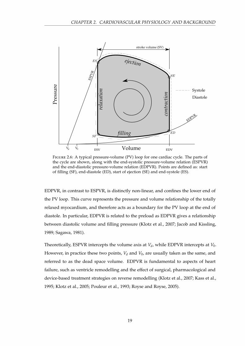
2.6 A typical pressure-volume (PV) loop for one cardiac cycle. The parts ofthe cycle are shown, along with the end-systolic pressure-volume relation(ESPVR) and the end-diastolic pressure-volume relation (EDPVR). Pointsare defined as: start of filling (SF), end-diastole (ED), start of ejection(SE) and end-systole (ES). . . . . . . . . . . . . . . . . . . . . . . . . . . . 19
2.7 An illustration of changing preload, increasing from loop A to loop B.Stroke volume and EDV increase, while contractility (slope of ESPVR)and afterload (Ea) remain constant. Points are defined as: start of filling(SF), end-diastole (ED), start of ejection (SE) and end-systole (ES). . . . . 21
2.8 An illustration of changing afterload, increasing from loop A to loopB. Points are defined as: start of filling (SF), end-diastole (ED), start ofejection (SE) and end-systole (ES). . . . . . . . . . . . . . . . . . . . . . . 23
2.9 Contractility as measured off a PV loop, increasing with, in this case,an increased stroke volume and pulse pressure. Contractility is theslope of the line joining Vd and the point of end-ejection. Points aredefined as: start of filling (SF), end-diastole (ED), start of ejection (SE)and end-systole (ES). . . . . . . . . . . . . . . . . . . . . . . . . . . . . . . 24
2.10 The relationship between cardiac output (CO) and end-diastolic pressure(EDP), which is the basis of the Frank-Starling law, source (Burkhoff, 2002). 25
2.11 The propagation channels of the electrical activation of the heart muscle. 262.12 A idealised illustration of a typical healthy ECG trace, showing the P, R,
Q, S and T points of the trace. . . . . . . . . . . . . . . . . . . . . . . . . . 27
3.1 A Windkessel model and a three-element series electrical representation.This is the basic compartment or element model from which the overallCVS model is derived. . . . . . . . . . . . . . . . . . . . . . . . . . . . . . 41
xv
LIST OF FIGURES
3.2 The schematic model and its electrical circuit equivalent. Note thatfor simplicity the ventricle interaction through the septum is not fullydescribed in the electrical equivalence. . . . . . . . . . . . . . . . . . . . . 42
3.3 A single elastic chamber shown in isolation. P is pressure, E the elastance,V the volume, Vd the unstressed volume and Q is the flow. . . . . . . . . 43
3.4 The representation of a valve between two chambers. The valve ismodelled as a diode, with resistance and inertial effects. . . . . . . . . . 44
3.5 Flow between elastic chambers with only resistance. . . . . . . . . . . . 453.6 The pressure-volume loop, as defined in Figure 2.6, showing ESPVR and
EDPVR as defined in Equations (3.16) and (3.17). . . . . . . . . . . . . . 473.7 The free wall concept, top graphic, showing the left and right free wall
volumes along with the septum free wall volume. The actual pressureand volume of the ventricles and surroundings are shown in the lowergraphic. . . . . . . . . . . . . . . . . . . . . . . . . . . . . . . . . . . . . . . 49
3.8 A single heart beat from a simulation of the model. The parameterswere chosen to resemble a healthy porcine subject, with a measuredtime-varying elastance. Pressure in the ventricle and downstream vesselare shown for each side of the heart, including the ventricle volume. . . 59
4.1 The full six-chamber model of the cardiovascular system as outlined inChapter 3. . . . . . . . . . . . . . . . . . . . . . . . . . . . . . . . . . . . . 66
4.2 The model in pictorial form, split into two sub-models, the systemicand pulmonary models. Each sub-model has external bounds whichoverlap, namely the vena cava pressure (Pvc), and the pulmonary veinpressure (Ppu). These overlapping chambers are no longer elastic, andthus the two respective pressures are constant with respect to time. Thetwo contractilities, Ees,lvf and Ees,rvf are also used to couple the modelstogether. The parameters to be identified are shown, including the leftand right time-varying elastances. . . . . . . . . . . . . . . . . . . . . . . 72
4.3 The identification of the systemic model with three points of iteration.The model is given seven parameter values and the time-varying elas-tance of the left ventricle, and returns five modified, and converged,parameter values. . . . . . . . . . . . . . . . . . . . . . . . . . . . . . . . . 74
4.4 The identification of the pulmonary model with three points of iteration.The model is given seven parameter values and the time-varying elas-tance of the right ventricle, and returns five modified, and converged,parameter values. . . . . . . . . . . . . . . . . . . . . . . . . . . . . . . . . 76
4.5 The modified version of the model that is used to identify the venouschamber elastances. This model is identical to the full six-chamber exceptfor one aspect, the pulmonary vein pressure is held constant, turning thesix-chamber model into a five chamber model. . . . . . . . . . . . . . . . 79
4.6 Six different time-varying elastances. A: The measured time-varyingelastance, B: the time-varying elastance constructed as a sum of Gaussianterms (Chung et al., 1997; Starfinger, 2008), C: the time-varying elastanceused in the original implementation of the model (Smith, 2004), D: a‘universal’ time-varying elastance (Suga et al., 1973), E: square wave, withsmoothed corners, F: a piecewise linear, five-segment representation ofthe time-varying elastance, also with smoothed corners. . . . . . . . . . 82
xvi
LIST OF FIGURES
4.7 The left ventricle pressure output of the model using the six differenttime-varying elastances of Figure 4.6. . . . . . . . . . . . . . . . . . . . . 85
4.8 The aortic pressure output of the model using the six different time-varying elastances of Figure 4.6. . . . . . . . . . . . . . . . . . . . . . . . 86
4.9 The pulmonary vein pressure output of the model using the six differenttime-varying elastances of Figure 4.9. . . . . . . . . . . . . . . . . . . . . 86
5.1 Left ventricular pressure-volume loops of a denervated heart, adaptedfrom (Suga et al., 1973). The arterial pressure was fixed at three differentlevels, for each of a control state and an enhanced contractile state. . . . 92
5.2 Isochrone regression lines at times, t0, t1, t2 and t4, all connected tothe dead space volume, Vd (left), and the equivalent time points on thetime-varying elastance curve (right). . . . . . . . . . . . . . . . . . . . . . 94
5.3 A one (left) and three (right) element time-varying elastance model. Theload, when applied to the cardiovascular context, is the arterial load. . . 95
5.4 The total mechanical energy for a contracting ventricle as representedby the sum of the work done by the ventricle (light grey area) and thepotential energy remaining in the muscle at the end of systole (dark greyarea). . . . . . . . . . . . . . . . . . . . . . . . . . . . . . . . . . . . . . . . 99
6.1 The figure shows a conceptualised overview of the process described inthis chapter and Chapter 7, and further implications. From the manymeasured left ventricular time-varying elastance waveforms, elv(t), alongwith many aortic pressure waveforms, Pao, correlations are derived —the information flow is shown through the large grey arrow. Once thesecorrelations are known, they can be used along with the aortic pressurewaveform (from a specific patient), to arrive at an estimation of theirtime-varying elastance waveform. The equivalent for the right side isalso shown. . . . . . . . . . . . . . . . . . . . . . . . . . . . . . . . . . . . 105
6.2 To illustrate what can be done with the identified points on the aorticpressure, an example of the formation of the estimated time-varyingelastance elastance is shown here, while the terms are defined in Equa-tion (6.1). . . . . . . . . . . . . . . . . . . . . . . . . . . . . . . . . . . . . . 105
6.3 A representative aortic pressure waveform over one heart beat withrelevant points, defined in Equation (6.1), marked on it. The two dashedcircles, MN and RS are used only in locating other points. . . . . . . . . 106
6.4 A representative pulmonary artery pressure waveform over one heartbeat with relevant points, defined in Equation (6.1), marked on it. Thedashed circle, MX is used only to help find other points. . . . . . . . . . 106
6.5 An illustration of the shear transformation of Equation (6.2), turning ahard to locate “shoulder”, B, into an easily found maximum point B. . 108
6.6 The desired point for MN is P. However, in this example the globalminimum of the waveform is P1, which is the initial estimation for MN.A shear transform of the pressure waveform between P1 and MX revealsa minimum (P2) outside the range of D, thus P2 is taken as the time ofMN. . . . . . . . . . . . . . . . . . . . . . . . . . . . . . . . . . . . . . . . . 110
6.7 This example is the other situation in the process of finding MN toFigure 6.6, i.e. the initial estimation of the global minimum for MN iscorrect. Here, the minimum of the shear transform from P1 to MX fallswithin the range of D, thus the P1 is taken as MN. . . . . . . . . . . . . . 111
xvii
LIST OF FIGURES
6.8 A straight forward case for finding DMPG, where P1 of Equation (6.13)exists, thus DMPG ≡ P1. . . . . . . . . . . . . . . . . . . . . . . . . . . . . 114
6.9 A less common case for finding DMPG, where P1 of Equation (6.13)does not exist, but P3 does, thus DMPG ≡ P3. . . . . . . . . . . . . . . . 114
6.10 A less common case for finding DMPG, where P1, and P3 of Equa-tion (6.13) do not exist, but P4 does, thus DMPG ≡ P4. . . . . . . . . . . 115
6.11 An example of where the first local minimum of the shear transform isthe correct time for the point DN. . . . . . . . . . . . . . . . . . . . . . . 117
6.12 Ppa alongside the matching time-varying elastance. The automatic oralgorithmic method failed to capture the correct DN point, locating apoint too late in the waveform (circle), the real DN and associated MXare marked by squares. . . . . . . . . . . . . . . . . . . . . . . . . . . . . . 119
7.1 An overall description of the method presented in this chapter, show-ing the left and right TVE waveforms with the four points requiredto reconstruct them, along with the origin of these values on the pres-sure waveforms. The large hollow arrows show the general flow ofinformation, while the smaller arrows show more fine-grained flow. . . 127
7.2 A simple high-level overview of the method within this chapter. Itcan be divided into two parts, the first involves the preparation of thecorrelations from invasively measured metrics, the second, a clinicalmethod for use in an intensive care setting. . . . . . . . . . . . . . . . . . 128
7.3 An example of a typical time-varying elastance broken into its mainsections, an exponential rise (A), decay (C) and a near linear section inbetween (B). . . . . . . . . . . . . . . . . . . . . . . . . . . . . . . . . . . . 130
7.4 An example of the calculation of the error metric. At each point on thetrue waveform, the nearest point on the estimated waveform is located,and the distance between these two points is calculated (draw as solidlines). This is an approximation of the normal distance between the twowaveforms. From this series of error values along the waveform, medianand 90th percentile errors are calculated. . . . . . . . . . . . . . . . . . . . 134
7.5 Three correlations are shown for each of the left (top row), and the righttime-varying elastance (bottom row). These three represent the best (left),median (middle) and worst (right) correlations by R value. The medianand worst case for the right time-varying elastance are multi-variablecorrelations, and therefore only a visualisation, so they cannot be usedto read off data in the way a single variable correlations graph can. . . . 136
7.6 Results of the estimation of the time-varying elastance alongside thecorresponding measured elastance, for both pulmonary embolism (toprow) and septic shock (bottom row). For both conditions, the 10th, 50th
and 90th percentile cases, by median error, are shown in positions left,middle and right respectively. . . . . . . . . . . . . . . . . . . . . . . . . . 139
7.7 Four reconstructions of the left and right time-varying elastance, fromthe same pig, as the pulmonary embolism progresses from healthy att = 0 to the end of trial at t = 260. . . . . . . . . . . . . . . . . . . . . . . 140
8.1 The left time-varying elastance, elv, and Pao showing the relationshipbetween them and specific points on both waveforms. . . . . . . . . . . 147
8.2 Method for directly measuring a value for afterload on the left ventriclepressure-volume loop. . . . . . . . . . . . . . . . . . . . . . . . . . . . . . 148
xviii
LIST OF FIGURES
8.3 The correlation for estimating afterload, in the septic shock and pul-monary embolism cohorts separately. . . . . . . . . . . . . . . . . . . . . 151
8.4 The correlation for estimating afterload in the combined septic shockand pulmonary embolism cohorts. . . . . . . . . . . . . . . . . . . . . . . 151
8.5 Estimating afterload on the pulmonary embolism and septic shock co-horts, based on estimators created on the combined cohort, of Figure 8.4. 152
8.6 The correlation for estimating Rsys, in the septic shock and pulmonaryembolism cohorts separately. . . . . . . . . . . . . . . . . . . . . . . . . . 153
8.7 The correlation for estimating Rsys in the combined septic shock andpulmonary embolism cohorts. . . . . . . . . . . . . . . . . . . . . . . . . . 154
8.8 The correlation between the mean aortic pressure and the point Pao(DMPG),with a correlation coefficient of R = 0.985. . . . . . . . . . . . . . . . . . 154
8.9 Estimating Rsys on the pulmonary embolism and septic shock cohorts,based on estimators created on the combined cohort, of Figure 8.7. . . . 155
8.10 The correlation for estimating Rpul in the septic shock and pulmonaryembolism cohorts, separately. . . . . . . . . . . . . . . . . . . . . . . . . . 156
8.11 The correlation for estimating Rpul in the combined septic shock andpulmonary embolism cohorts. . . . . . . . . . . . . . . . . . . . . . . . . . 157
8.12 Estimating Rpul on the pulmonary embolism and septic shock cohorts,based on estimators created on the combined cohort, of Figure 8.11. . . 158
xix


List of Tables
2.1 The range of systemic inflammatory response syndromes, summarisedfrom (Annane et al., 2005). . . . . . . . . . . . . . . . . . . . . . . . . . . . 32
3.1 The analogous metrics between the electrical domain and fluid dynamicsalong with their typical symbols, and units in each system. . . . . . . . 38
3.2 The analogous components between the electrical domain and fluiddynamics along with their typical symbols. . . . . . . . . . . . . . . . . . 39
3.3 Model input parameters for the six-chamber cardiovascular model alongwith units and healthy values. . . . . . . . . . . . . . . . . . . . . . . . . 55
3.4 The outputs of the model along with their respective numerical units. . 57
4.1 The parameters of the six-chamber model along with their initial values,surrogate errors and the sub-model in which they are used. . . . . . . . 73
4.2 The allowable range of values for the parameters of the six-chambermodel. Each parameter is restricted in the identification to be within thisrange, to insure the parameters are physiologically meaningful. . . . . . 81
4.3 The parameters used for Equation (4.23). . . . . . . . . . . . . . . . . . . 83
6.1 The step by step method for finding the points on Pao and Ppa, as labelledon the right. The graphics beside each step are for illustration onlyand are not meant to be part of the definition of the method, ratherthey are to demonstrate the method in operation on a representativePao waveform. Note that the methods described here for DMPG andDN are not complete as these require a more complex method. Refer toSections 6.4.1 and 6.4.2 for the complete method for these two points. . 112
6.2 Accuracy of the method: number of points grouped by absolute error(of 88 total points). ∗ note that the validation of LS here is partially selffulfilling and is included here only for completeness. . . . . . . . . . . . 119
7.1 Reconstruction formulae for the three different types of correlations usedto estimate the time-varying elastance. . . . . . . . . . . . . . . . . . . . . 132
7.2 Correlations for points on the left ventricle elastance. All points usecorrelation α defined in Table 7.1. . . . . . . . . . . . . . . . . . . . . . . . 135
7.3 Correlations for points on the right ventricle elastance. The differentformulae, for the column ‘Type’, are defined in Table 7.1. . . . . . . . . . 137
7.4 Percentage errors in the reconstructed driver functions, for pulmonaryembolism and septic shock, using correlations derived from the wholecohort of 85 datasets. . . . . . . . . . . . . . . . . . . . . . . . . . . . . . . 138
xxi

LIST OF TABLES
7.5 Percentage errors in the reconstructed driver functions, for pulmonaryembolism and septic shock, for the independent cross validation usingcorrelations derived from the alternative trial of cardiac dysfunction. . . 138
xxii

Nomenclature
Acronyms
AL Afterload
AP Arterial pressure
CO Cardiac output
CT Computer tomography
CVP Central venous pressure
CVS Cardiovascular system
DVT deep venous thrombus
ECG Electrocardiogram
ED End-diastole
EDP End-diastolic pressure
EDPVR End-diastolic pressure-volume relation
EDV End-diastolic volume
ES End-systole
ESPVR End-systolic pressure-volume relation
ESV End-systolic volume
GEDV Global end-diastolic volume
xxiii

LIST OF TABLES
HR Heart rate
ICU Intensive Care Unit
LSV Left stroke volume
LVEDV Left ventricle end-diastolic volume
MAP Mean arterial pressure
PAC Pulmonary artery catheter
PAC Pulmonary artery catheter
PAP Pulmonary artery pressure
PE Pulmonary embolism
PE Pulmonary embolism
PP Pulse pressure
PV Pressure-volume
PVA Pressure-volume area
RMSE Root mean square error
RSV Right stroke volume
RV Right ventricle
RVEDV Right ventricle end-diastolic volume
SE Start of ejection
SF Start of filling
SIRS Systemic inflammatory response syndrome
SV Stroke volume
TVE Time-varying elastance
V/Q Ventilation-perfusion scintigraphy
xxiv

LIST OF TABLES
VTE venous thromboembolism
Roman Symbols
C Compliance
E Elastance
I Inertia
P Pressure
Q Flow rate
R Resistance
T Period
t Time
V Volume
Greek Symbols
H Half rectifier
φshear The shear transform function
Other Symbols
S Shear transform
CO2 Carbon Dioxide
X The mean value of X
DMPG Driver maximum positive gradient
DN Dicrotic notch
E(t) Time-varying elastance — general concept
e(t) Time-varying elastance, value normalised
xxv

LIST OF TABLES
LS Left shoulder
MN Minimum point
MNG Maximum negative gradient
MPG Maximum positive gradient
MX Maximum
O2 Oxygen
RS Right shoulder
Subscripts
ao Aorta
approx The approximated value
av Aortic valve
ed End-diastole
end The final value of a data set
est The estimated value
es End-systole
fm Five chamber model
lvf Left ventricle free wall
lv Left ventricle
max Maximum value
measured Value from the measured data
min Minimum value
modelled Value from the model’s output
mt Mitral valve
xxvi

LIST OF TABLES
pa Pulmonary artery
pcd Pericardial difference
peri Pericardium
pul Pulmonary
pu Pulmonary vein
pv Pulmonary valve
rvf Right ventricle free wall
rv Right ventricle
sm Systemic model
spt Ventricular septum
sum Summation of parameters
sys Systemic
tc Tricuspid valve
th Thoracic
true The true value
vc Vena cava
v Ventricle
a Arterial
xxvii


Chapter 1
Introduction
Cardiac disturbances are difficult to diagnose and treat, especially in an Intensive Care
Unit (ICU), which can lead to poor management (Hall and Guyton, 2011; Grenvik et al.,
1989). Inadequate diagnosis is common, and plays a significant role in increased length
of stay and death (Angus et al., 2001; Kearon, 2003; Pineda et al., 2001), despite access to
many different cardiac measurements and metrics. Currently, internal haemodynamic
measurements are possible only at the arterial or venous locations where catheters
are placed. This limited set of data can severely restrict clinical diagnostic capability.
In addition, they return pressure or flow rate waveforms that provide a wealth of
information, but not in a form that easily matches the mental models of clinical staff.
Thus, the use of these catheters is not necessarily associated with improved outcomes
(Frazier and Skinner, 2008; Chatterjee, 2009; Cooper and Doig, 1996). Overall, a lot of
data currently available to ICU clinicians that could have significant clinical value is
under utilised.
Using computer modelling techniques, this limited set of data can be expanded to esti-
mate a much greater set of clinically and physiologically relevant data to enable more
accurate diagnosis. For example, acute cardiovascular dysfunctions, like pulmonary
embolism (PE) and septic shock, severely alter cardiovascular system (CVS) haemody-
namics around the heart. These changes can be seen by catheter measurements as a
change in the balance of preload and afterload around the heart, resulting in an altered
cardiac energetic state (Weber and Janicki, 1979; Ross, 1976). Detailed cardiac energetics
are too invasive to measure in an ICU setting. However, if the relevant energetics could
1

1.1. CARDIOVASCULAR DISEASE
be captured from a nearby catheter with the use of a physiologically relevant computer
model, then the clinical potential of such measurements could be realised. To date, no
such method achieves this aim.
1.1 Cardiovascular disease
The prevalence and cost of cardiovascular disease is an enormous problem, and one
that is not new. In every year since 1900, except 1918, cardiovascular disease was the
leading cause of death in the United States (Roger et al., 2012). In 2008, it was the
biggest cause of death worldwide, with more than 17 million casualties (Mendis et al.,
2011), of which an estimated three million could have been prevented. Similarly in
2008, cardiovascular disease was the underlying cause of just under one third of all
deaths in the United States, and contributed to over half of all deaths. Currently, it is
estimated that nearly 83 million American adults, more than a third of the population,
have one or more types of cardiovascular disease (Roger et al., 2012).
It is also apparent that cardiovascular disease can effect all age groups. Although age
is still an important risk factor in developing cardiovascular disease, the prevalence of
cardiac dysfunction is showing a worrying trend in youth populations (McGill et al.,
2008). In particular, an estimated nearly six thousand paediatric out-of-hospital cardiac
arrests occur annually in the United States alone (Roger et al., 2011).
Aside from the human cost and social ramifications of cardiovascular disease, the
economic cost is also significant. It is estimated that the total direct and indirect cost of
cardiovascular disease in the United States in 2008 was a massive $297 billion (up $11
billion from the previous year), which is the highest of any diagnostic group (Roger
et al., 2011, 2012). This value is expected to reach $818 billion by 2030 (Heidenreich et al.,
2011). This cost is a heavy burden on the economy, as well as on hospital resources,
with nearly 7.5 million inpatient cardiovascular operations and procedures performed
in 2009 in the United States alone (Roger et al., 2012).
Overall, it is clear that cardiovascular disease is a serious human and economic problem,
growing in epidemic proportions worldwide. Even small advances in diagnosing and
treating cardiovascular disease would see significant benefits in reduced mortality
and financial savings. However, due to many factors, including the complexity of
2
CHAPTER 1. INTRODUCTION
the cardiovascular system, diagnosis and optimal treatment is often very difficult. In
particular, severe sepsis and septic shock, which have high occurrence rates, significant
mortality and costs (Karlsson et al., 2007), continue to be difficult to manage in an ICU,
and reflect the overall issues of occurrence and cost of cardiovascular disease in general
within this hospital environment.
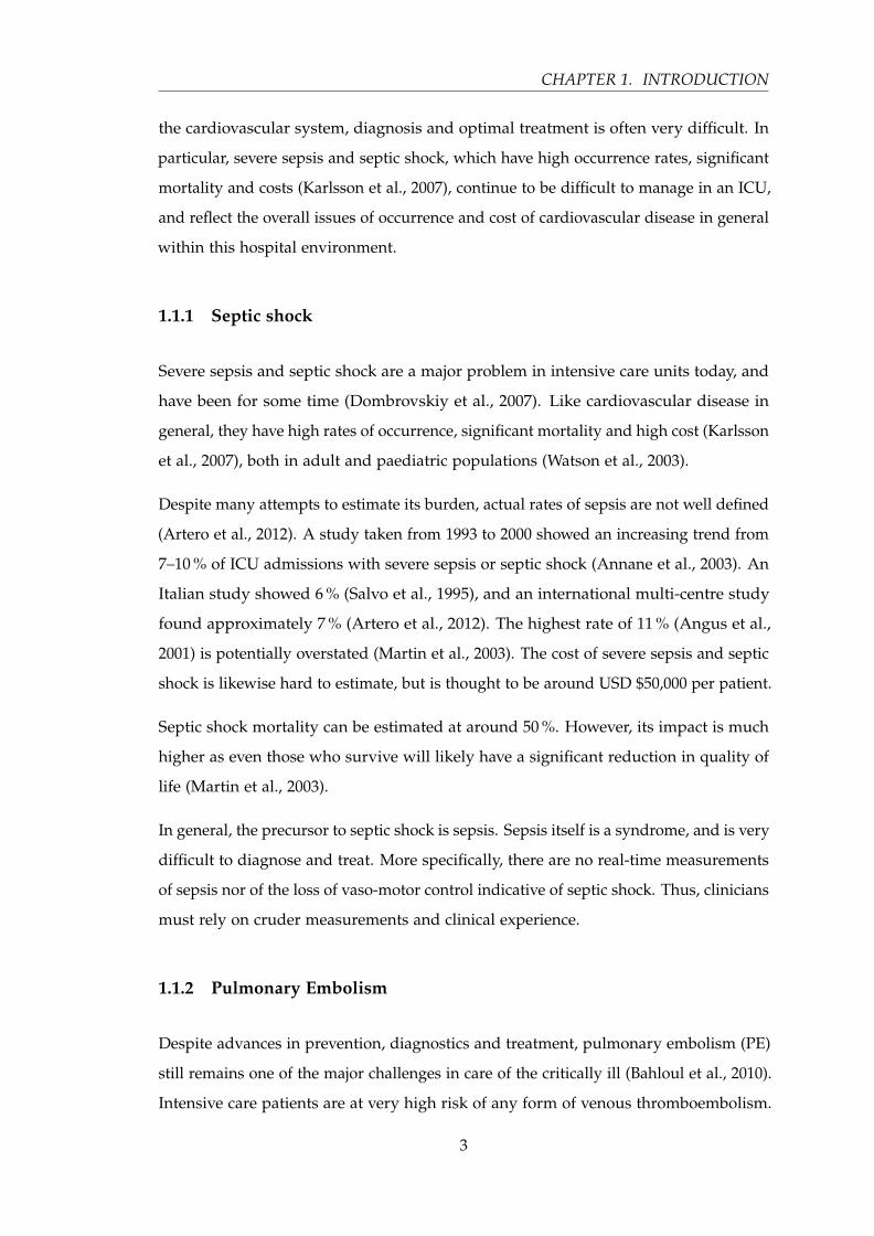
1.1.1 Septic shock
Severe sepsis and septic shock are a major problem in intensive care units today, and
have been for some time (Dombrovskiy et al., 2007). Like cardiovascular disease in
general, they have high rates of occurrence, significant mortality and high cost (Karlsson
et al., 2007), both in adult and paediatric populations (Watson et al., 2003).
Despite many attempts to estimate its burden, actual rates of sepsis are not well defined
(Artero et al., 2012). A study taken from 1993 to 2000 showed an increasing trend from
7–10 % of ICU admissions with severe sepsis or septic shock (Annane et al., 2003). An
Italian study showed 6 % (Salvo et al., 1995), and an international multi-centre study
found approximately 7 % (Artero et al., 2012). The highest rate of 11 % (Angus et al.,
2001) is potentially overstated (Martin et al., 2003). The cost of severe sepsis and septic
shock is likewise hard to estimate, but is thought to be around USD $50,000 per patient.
Septic shock mortality can be estimated at around 50 %. However, its impact is much
higher as even those who survive will likely have a significant reduction in quality of
life (Martin et al., 2003).
In general, the precursor to septic shock is sepsis. Sepsis itself is a syndrome, and is very
difficult to diagnose and treat. More specifically, there are no real-time measurements
of sepsis nor of the loss of vaso-motor control indicative of septic shock. Thus, clinicians
must rely on cruder measurements and clinical experience.
1.1.2 Pulmonary Embolism
Despite advances in prevention, diagnostics and treatment, pulmonary embolism (PE)
still remains one of the major challenges in care of the critically ill (Bahloul et al., 2010).
Intensive care patients are at very high risk of any form of venous thromboembolism.
3

1.2. CURRENT PRACTICE
Combined with the often non-specific nature of the visible effects of PE, it becomes
clear why PE is another leading cause of in-hospital morbidity and mortality (Tapson,
2008; Kasper et al., 1997; Konstantinides et al., 1997). Mortality rates vary widely, from
8.1 % in stable patients to 65 % in post-cardiopulmonary resuscitation (Goldhaber et al.,
1999; Kasper et al., 1997; Douketis, 2001). It is also a widespread problem with an
incidence rate of 1 per 2000 person-years (Naess et al., 2007). Hence, it is another high
cost, frequently occurring cardiovascular dysfunction for which proper diagnosis and
optimal treatment are difficult.
1.1.3 Diagnosis and Treatment
The treatment of cardiovascular disease is not a simple task. This issue is due to many
factors including the complexity of the cardiovascular system and the patient-specific
nature of the cardiac related problems. Both diagnosis and treatment can thus be
problematic. In particular, there is no direct measurement of thromboembolism or
blocking of blood flow that is currently available in real-time. Thus, clinicians often
have to rely on experience and intuition, using cruder surrogates, to make a diagnosis
or to recognise PE as it emerges. This situation leads to increased clinical errors and
suboptimal patient outcomes.
Hence, overall, diagnosis of many cardiovascular dysfunctions are non trivial. The
complexity of the cardiovascular system, interactions and complex reflex responses
result in conditions that can be difficult to reliably and accurately diagnose in a timely
fashion. This issue is further complicated by patient-specific differences and responses
to conditions and treatments. Finally, the measurements available are not entirely
physiologically relevant to clinical or specific dysfunction. The resulting situation for
a clinician is often that of intuition plus trial and error, leading to suboptimal and
variable diagnosis and treatment.
1.2 Current practice
The ICU provides care for patients who are the most critically ill in the hospital. Thus,
the clinical staff are often faced with hard decisions in stressful and time-sensitive
4

CHAPTER 1. INTRODUCTION
situations. There are many procedures and methods to enable staff to make good
decisions in specific situations or treatments. However, much of the time these methods
are optimised for population outcomes, which can result in patient-specific details
being neglected. The result is more consistent care, but not necessarily more optimal
care.
In addition, all patients have their own unique expressions of a cardiovascular disease
or dysfunction, as well as unique responses to treatment. This variability and resultant
uncertainty leaves the clinician with a vast array of scenarios and data to mentally
process including the patient’s history, their current cardiovascular state, their current
response to treatment, and the results of the vast quantity of invasive and non-invasive
clinical studies. The result is often an array of sometimes conflicting possible treatments
paths. With this issue in mind, it is no surprise that clinical management and patient
outcomes vary between medical centres (Kennedy et al., 2010; Wennberg, 2002), and
that clinical error rates are common (Abramson et al., 1980; Donchin et al., 1995; Morris,
2001; Suresh et al., 2004)
For much of the treatment in the ICU, haemodynamic monitoring is a first port of call.
However, for any monitoring to improve outcome, the information gained must then
direct or influence treatment, and only in beneficial ways. For this reason, the use of the
pulmonary artery catheter (PAC) is declining worldwide due to the lack of improved
patient outcomes (Wiener and Welch, 2007). Many variables are still monitored as
part of standard practice, resulting in a wealth of patient-specific haemodynamic
information, much of which is not fully utilised in treatment decisions (Pinsky, 2003;
Greenberg et al., 2009). Too much information can lead to confusing and apparent
contradictory diagnostic and treatment paths, and may be no better than an incomplete
understanding due to too little information. This problem can be seen through the
apparent lack of improved patient outcomes from the monitoring of stroke volume and
cardiovascular output using a PAC (Mutoh et al., 2007; Pinsky, 2007; Greenberg et al.,
2009) despite their importance to the state of cardiovascular health.
To fully utilise the information gained by haemodynamic monitoring, this information
must be aggregated into a simpler, yet more complete picture of the cardiovascular
system. Without this clearer picture the wealth of relevant clinical information in
monitored variables is far too large, and the interaction too complex for the clinician to
5
1.3. TIME-VARYING ELASTANCE
form a clear, concise understanding of the patient-specific cardiovascular state upon
which to base treatment decisions. Historically, this type of outcome has been best
achieved through the use of computer models (Le Compte et al., 2009; Chase et al.,
2008; Evans et al., 2011). Such models can incorporate complex interactions, and distil
the large quantity of monitored information into manageable and understandable infor-
mation that can be standardised, yet remain patient-specific. To be clinically applicable,
such models should be able to accurately predict cardiovascular health markers, track
pathologically important haemodynamic trends, indicate the effectiveness of treatment
over time, be cost effective and easy to implement, provide real-time information, and
improve current clinical methods and outcomes.
1.3 Time-varying elastance
For many of the cardiovascular models developed in the literature, an important input
function is the time-varying elastance (TVE) waveform. This waveform describes the
energetic input to the contracting ventricles and, as such, drives the pumping action
of the models. Furthermore, due to the centrality of the time-varying elastance and
the energetic implications, the waveform is useful in its own right. However, the
time-varying elastance is impractical to measure in a clinical setting. Thus, it has not
reached clinical practice to the extent it is seen in animal research and clinical textbooks.
There have been several attempts to estimate TVE (Guarini et al., 1998; Swamy et al.,
2009; Shishido et al., 2000; Senzaki et al., 1996; Brinke et al., 2010). However, none
have estimated it for its own sake. Most studies present a method using the TVE to
estimate a specific clinical parameter, most commonly end-systolic elastance (Shishido
et al., 2000; Brinke et al., 2010; Senzaki et al., 1996) and ejection fraction (Swamy et al.,
2009). However, their validation is based on these metrics, which in turn capture
cardiovascular state at a specific instant, and not on the resulting TVE waveform.
1.4 Goals for this research
The overall goal of this research is to further the clinical applicability of a relatively
minimal cardiovascular system model (Starfinger, 2008). This model can be fitted to
6

CHAPTER 1. INTRODUCTION
capture the behaviour of a specific patient and thus give accurate information to the
clinician about the patient’s cardiovascular state. For this outcome to be clinically
relevant, it must be possible for the model to be identified to simulate a specific patient
and to do that in a real-time fashion. It also must be done through the use of only
measurements that are typically available in the ICU, so as to not add additional cost
or risk to the patient.
These criteria require a validated and accurate model, and a method to convert the
limited measured data that is available in the ICU into the required parameters for the
model to match a specific patient. Along with this requirement is the necessity for an
accurate representation of the time-varying elastance (TVE) waveform, as this waveform
is a central input to the model and is too invasive to measure directly. Therefore, the
estimation of the TVE is critical to the success of the model as a clinical tool, and thus
the TVE waveform is the main focus of this research.
1.5 Preface
In Chapter 2 this thesis will cover the background material necessary to fully under-
stand the concepts, models and physiology mentioned in this research. This background
includes the physiology and anatomy of the heart and circulation system, as well as the
clinically relevant metrics and concepts that are discussed in later chapters. This chapter
also covers the major cardiac dysfunctions relevant to this research, their pathologies,
current diagnostic methods and typical treatment paths.
Chapter 3 will introduce and define the lumped cardiovascular system model, giving a
basic demonstration of its derivation, guiding principles and background philosophy
and direction, including a full definition of the model. The simulation of the model
will also be discussed along with the assumptions and limitations of the model. The
process of identifying the model is then shown in Chapter 4, where the iterative process
is outlined. Also discussed is the sensitivity of the model to the time-varying elastance
input waveform.
Chapter 5 then introduces the time-varying elastance in much more detail, outlining
the evolution of this concept from its inception in the 1960s to its current usage and
7

1.5. PREFACE
implications today, including the relevant literature. The three major uses of the time-
varying elastance are covered, namely the maximal elastance, total mechanical energy
formulation from the pressure-volume diagram and the time-varying elastance as an
input to lumped parameter cardiovascular models.
With this background in place, Chapters 6 and 7 outline and discuss the method by
which the time-varying elastance can be accurately estimated using only measurements
that are typically available in an ICU setting. This process involves the automation of
the processing of the input waveforms to obtain the required data, and is shown in
Chapter 6. This is followed by the method of estimating the time-varying elastance
from the processed data, and is discussed in Chapter 7.
Chapter 8 follows this estimation with the clinical relevance of the time-varying elas-
tance apart from the cardiovascular model. Three correlations are proposed that can
give further insight into the cardiovascular state, in a similar way to the full cardiovas-
cular model, without the computation cost involved in identifying and simulating the
full model.
Finally, Chapter 9 gives an overall summary and conclusions of this research, with
future work that could be done next around this topic, discussed in Chapter 10.
8
Chapter 2
Cardiovascular Physiology and
Background
This chapter introduces the anatomy and physiology behind the cardiac and circulation
systems. It provides the background information for which the later chapters assume a
working knowledge.
2.1 Anatomy of the heart
The heart primarily consists of two separate pumps, the left heart which pumps
oxygenated blood to the body’s periphery, and the right heart which pumps blood
to the lung to be re-oxygenated. Each side of the heart contains a main pump, the
ventricle, and a much weaker upstream pump, the atrium. The left and right ventricle
share a common wall, called the interventricular septum, and thus are in direct contact
and interact in terms of pressure and volume. The entire heart is enclosed by the
pericardium, a stiff membrane that constrains the total volume of the heart. Figure 2.1
shows a representation of the heart and connection vessels.
2.1.1 Heart chambers
There are four active chambers in the heart that contribute to the pumping of blood.
These are the left and right atria, and the left and right ventricles. All four interact on
9

2.1. ANATOMY OF THE HEART
Figure 2.1: A diagram of the heart. Patrick J. Lynch. Adapted under CreativeCommons Attribution 2.5 License.
each side to create a full cardiac cycle. These chambers are shown in Figure 2.2.
The left atrium receives blood from the lungs, and through the bicuspid valve, delivers
it to the left ventricle to be pumped through the systemic circulation. The left ventricle
operates at high pressure against significant resistance. Hence it has strong, thick walls
and a circular lumen.
The right atrium takes blood from the superior and inferior venae cavae and the
10

CHAPTER 2. CARDIOVASCULAR PHYSIOLOGY AND BACKGROUND
Figure 2.2: An illustration of a sectioned heart. Patrick J. Lynch. Adapted underCreative Commons Attribution 2.5 License.
coronary sinus, and delivers it to the right ventricle, through the tricuspid valve. The
right ventricle, operating at a much lower pressure than the left ventricle, then pushes
this blood into the pulmonary circulation through the pulmonary valve. The right
ventricle has thinner walls, and a less circular lumen.
The left and right ventricles are connected by the interventricular septum, and are
thus dynamically linked. This interaction can be important in certain disease states or
dysfunction. Section 2.1.3 has a full description.
2.1.2 Cardiac muscle
The walls of the heart consist of three layers: the epicardium, myocardium and endo-
cardium. The epicardium is the thin, outermost layer and houses the major coronary
blood vessels that supply the myocardium. The myocardium is composed of cardiac
11
2.1. ANATOMY OF THE HEART
muscle tissue and makes up the greater part of the heart wall’s thickness. The endo-
cardium is a smooth inner layer of the heart that helps to reduce surface friction of the
muscle.
There are three types of muscle that make up the heart: atrial muscle, ventricular
muscle and conductive muscle fibres. There is much in common between cardiac and
skeletal muscle. However, cardiac muscle is specialised in a number of ways. The atrial
and ventricular muscles are similar to one another and contract in a similar way to
skeletal muscle, whereas the conductive muscles fibres do not contract much, as their
primary purpose is conduction.
Cardiac muscle contraction differs slightly from skeletal muscle in two main ways.
Specifically, it has longer action potential and exhibits a plateau after the initial spike.
This prolonged action potential and plateau are caused in part by the addition of slow
calcium channels (Tortora and Derrickson, 2011). Both types of muscles have the fast
sodium channels which remain open for a very short time allowing sodium ions to
enter the muscle. The slow calcium channels are slower to open and remain open for
longer, allowing both calcium and sodium to flow into the cardiac muscle maintaining
a prolonged depolarisation. A second cause of the difference between skeletal and
cardiac muscle is the permeability to potassium, which, in cardiac muscle, drastically
reduces during the polarisation. This reduction decreases the loss of positively charged
potassium ions, helping to maintain an elevated voltage for longer than skeletal muscle.
At the close of the slow calcium channels, the permeability returns to normal, reducing
the voltage to its resting level. Finally, cardiac muscle (both atrial and ventricular) also
has a much slower action potential velocity, clocking in at around 0.3–0.5 m s−1, nearly
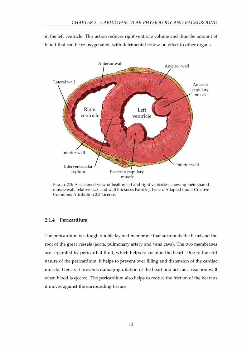
10 times slower than skeletal muscle.
2.1.3 Ventricular interaction
The left and right ventricles share a common boundary muscle, called the interven-
tricular septum. Hence, the dynamics of the two ventricles are closely linked. This
interaction is significant in a healthy heart, but can play a much greater role with certain
types of dysfunction, especially those that cause the pericardium to contract. Thus,
the status of the septum is important clinically. In particular, the septum is generally
pushed into the right ventricle, as shown in Figure 2.3, due to the much higher pressure
12
CHAPTER 2. CARDIOVASCULAR PHYSIOLOGY AND BACKGROUND
in the left ventricle. This action reduces right ventricle volume and thus the amount of
blood that can be re-oxygenated, with detrimental follow-on effect to other organs.
Figure 2.3: A sectioned view of healthy left and right ventricles, showing their sharedmuscle wall, relative sizes and wall thickness Patrick J. Lynch. Adapted under CreativeCommons Attribution 2.5 License.
2.1.4 Pericardium
The pericardium is a tough double-layered membrane that surrounds the heart and the
root of the great vessels (aorta, pulmonary artery and vena cava). The two membranes
are separated by pericardial fluid, which helps to cushion the heart. Due to the stiff
nature of the pericardium, it helps to prevent over filling and distension of the cardiac
muscle. Hence, it prevents damaging dilation of the heart and acts as a reaction wall
when blood is ejected. The pericardium also helps to reduce the friction of the heart as
it moves against the surrounding tissues.
13
2.2. CIRCULATION
2.2 Circulation
The circulation is the key mechanism for which the heart exists. The circulation, in
turn, serves the purpose of supplying the body with oxygen and nutrients, along with
other transport operations. It is the need for such transport that drives the function of
the circulation, its components, and ultimately, the heart itself.
There are three major parts to the circulation system: the arterial system, the venous
system and the capillary system. The arterial system transports the oxygenated blood
from the heart to the tissues at high pressure and high velocity, via arterioles and
ever-smaller branches of blood vessels, terminating with the capillaries. The capillaries
are where exchange of oxygen, nutrients and waste products mainly occur. The venous
system then returns blood to the heart at lower pressure and velocity.
2.2.1 Arterial system
The arterial system carries blood from the heart to the body’s organs, and comprises
three main forms: 1) elastic arteries, 2) muscular arteries, and 3) arterioles. As the blood
leaves the heart, it enters an elastic artery (the aorta for the left side, and pulmonary
artery for the right). These elastic arteries easily change volume in response to a change
of pressure, and thus have high compliance. Due to this high compliance, elastic
energy can be stored. This is then released to aid in propelling the blood through the
circulation system after the heart has finished its main pumping action. Hence, the
elastic arteries act as a pressure reservoir, and to elongate the pumping action over a
longer period into a more continuous waveform.
There are two major arteries that leave the heart, the aorta and the pulmonary artery.
The aorta takes oxygenated blood from the left side of the heart and supplies the body.
The pulmonary artery takes the de-oxygenated blood from the right side of the heart
and supplies it to the lungs to be re-oxygenated. These two arteries have significant and
important flow; they see the blood first after the heart, and can readily have catheters
placed for measurement.
After the elastic arteries have branched a few times, the blood moves into the muscular
arteries. These arteries are medium-sized with proportionally thicker walls than elastic
14
CHAPTER 2. CARDIOVASCULAR PHYSIOLOGY AND BACKGROUND
arteries and a consequent lower compliance, but are capable of actively dilating and
contracting to enable efficient blood flow and to help maintain blood pressure. These
vessels repeatedly branch, eventually distributing blood to the arterioles.
The arterioles are very small, but proportionally strong and thick walled vessels that
connect the arteries to the capillaries, and also regulate blood flow and pressure.
Arterioles range in size from 300 µm down to 15 µm. In contrast, muscular arteries
range from 4 mm to 0.5 mm and elastic arteries can be as large as 25 mm in diameter
(Martini et al., 2011).
2.2.2 Capillary system
Capillaries are the smallest blood vessels with diameters ranging from 5–10 µm, which
goes below the diameter of a single red blood cell (8 µm), and a wall thickness of only
a single layer of endothelial cells. The capillaries are the means by which substances
are diffused into and out of tissue, thus supplying nutrients and removing waste. This
exchange is made possible by the vast number (around 20 billion) of short capillary
vessels, distributed around the body to reach every tissue cell according to its nutrient
requirements.
2.2.3 Venous system
After the blood has travelled through the capillaries it then moves into the venous
system, starting with the venules. These are small, thin walled vessels, that, due to their
porous walls and proximity to the tissue, contribute significantly to the exchange of
nutrients and waste as well as to white blood cell emigration. As the veins get further
from the capillaries, the walls get thicker and more muscular, and diffusion with the
interstitial fluid stops. The venules, like the elastic arteries, have a high compliance and
thus can serve as a reservoir for large quantities of blood.
After the venules, the blood moves into the veins. The veins are thinned walled in
comparison to the arteries, but are otherwise of a similar structure. Their thin walls
reflect the significantly lower blood pressure in the venous system than the arterial
system. The main purpose of the veins is to return the blood to the heart, which is
15

2.2. CIRCULATION
helped by the skeletal muscles in the lower limbs and several valves to prevent the back
flow of blood.
2.2.4 Blood distribution
The veins and venules contain the largest proportion of blood, and act as a blood
reservoir. This reservoir can shrink and expand as needed to provide more or less
blood for active circulation. If more blood is needed for the skeletal muscles, the veins
and venules will contract (venoconstriction) pushing a greater percentage of blood
around the circulation system. Conversely, the veins and venules dilate to reduce the
flow and pressure of blood. Figure 2.4 shows a typical distribution of blood in a healthy
cardiovascular system at rest (Tortora and Derrickson, 2011).
Figure 2.4: The relative distribution of blood in the circulation system of an average,healthy, young adult at rest (Tortora and Derrickson, 2011).
2.2.5 Blood pressure and flow
The total blood flow at any given time is called the cardiac output (CO), and is the
product of the heart rate and stroke volume of each heartbeat. Typical values for male
and female humans is 5.6 L min−1 and 4.9 L min−1 respectively (Hall and Guyton, 2011).
Ultimately, the flow is a function of the vascular resistance and the pressure differential
16

CHAPTER 2. CARDIOVASCULAR PHYSIOLOGY AND BACKGROUND
across the systemic arteries, both of which are controlled by the body in various ways.
Cardiac output is regulated to ensure exchange of oxygen to tissues at a rate relative to
demand, which thus influences total blood flow and circulatory resistance or “tone”
(Hall and Guyton, 2011).
Blood pressure is a function of cardiac output, total blood volume and vascular
resistance, and in a relaxed young adult is approximately 110 mmHg (systolic) over
70 mmHg (diastolic). These values drop down to about 35 mmHg in the capillaries,
where the pulse fluctuations cease, and again to about 16 mmHg at the venules. This
overall level of blood pressure is represented in Figure 2.5.
Figure 2.5: A representation of the pressure of the left side of the circulation system,starting from the aortic artery, through the capillaries and ending where the venacava joins the heart. This chart is diagrammatic, and was adapted from Tortora andDerrickson (2011).
The vascular resistance is primarily a function of the lumen size, which is the internal
diameter of the vessel. The lumen size is controlled by the muscle fibres surrounding
the vessels. Hence, resistance, and thus resulting pressures, can be actively controlled.
More specifically, the whole system is controlled by negative feedback loops through
several different channels, neural feedback, hormonal feedback and autoregulation.
Neural feedback uses receptors located around the circulation system to give feedback
to the cardiovascular centre, at the base of the skull, which in turn responds to adjust the
17

2.3. MECHANICAL PROPERTIES OF THE HEART
pressure and flow. Baroreceptors respond to changes in pressure, while chemoreceptors
respond to changes in O2, CO2 and pH. Both these types of receptors have their most
important locations in the aorta and carotid sinus. Hormonal regulation works on the
release of certain types or hormones such as renin, epinephrine and norepinephrine
among others, which work on the heart and vessels to adjust their performance and/or
properties. Autoregulation, in contrast, is the ability of the tissue itself to adjust the
blood flow and pressure to suit its current needs (Tortora and Derrickson, 2011; Hall
and Guyton, 2011).
2.3 Mechanical properties of the heart
To date, the cardiac pressure-volume (PV) loop is one of the richest sources of infor-
mation about the heart. The diagram itself is simply a trace of the ventricle pressure
against the ventricle volume over a single cardiac cycle. From this diagram, many
different metrics can be seen or created, and many more arise from examining the
change in PV loops over time (Burkhoff et al., 2005; Suga, 1990a; Sagawa et al., 1988;
Moscato et al., 2007; Pacher et al., 2008). Figure 2.6 shows a typical (idealised) PV loop.
Three important metrics are shown in Figure 2.6, stroke volume (SV), end-systolic
pressure-volume relation (ESPVR) and end-diastolic pressure-volume relation (EDPVR).
The stroke volume is simply the difference in the volume of the ventricle over one
heart beat — the end-diastolic volume (EDV) minus the end-systolic volume (ESV). The
ESPVR and EDPVR are relationships that help define filling and ejection of the heart.
ESPVR, as the name suggests, is the relationship between pressure and volume at the
point of end-systole. This relationship was initially proposed to be linear (Weisfeldt
et al., 1976; Sagawa et al., 1977). However, more recent studies have shown that ESPVR
can be approximated as linear only within limits (Burkhoff et al., 1987; Krosl and
Abel, 1998; Noda et al., 1993). This relationship represents the pressure and volume
interaction of the maximally activated myocardium, and therefore provides a boundary
for the PV loop at the end of systole. The most important feature of this relationship
is the end-systolic elastance, Ees, which is the slope of this line. For more details on
ESPVR and its clinical significance, see Section 2.3.4.
18
CHAPTER 2. CARDIOVASCULAR PHYSIOLOGY AND BACKGROUND
Figure 2.6: A typical pressure-volume (PV) loop for one cardiac cycle. The parts ofthe cycle are shown, along with the end-systolic pressure-volume relation (ESPVR)and the end-diastolic pressure-volume relation (EDPVR). Points are defined as: startof filling (SF), end-diastole (ED), start of ejection (SE) and end-systole (ES).
EDPVR, in contrast to ESPVR, is distinctly non-linear, and confines the lower end of
the PV loop. This curve represents the pressure and volume relationship of the totally
relaxed myocardium, and therefore acts as a boundary for the PV loop at the end of
diastole. In particular, EDPVR is related to the preload as EDPVR gives a relationship
between diastolic volume and filling pressure (Klotz et al., 2007; Jacob and Kissling,
1989; Sagawa, 1981).
Theoretically, ESPVR intercepts the volume axis at Vd, while EDPVR intercepts at V0.
However, in practice these two points, Vd and V0, are usually taken as the same, and
referred to as the dead space volume. EDPVR is fundamental to aspects of heart
failure, such as ventricle remodelling and the effect of surgical, pharmacological and
device-based treatment strategies on reverse remodelling (Klotz et al., 2007; Kass et al.,
1995; Klotz et al., 2005; Pouleur et al., 1993; Royse and Royse, 2005).
19

2.3. MECHANICAL PROPERTIES OF THE HEART
2.3.1 Cardiac cycle
The cardiac cycle consists of four segments, distinct in their cardiac function, as shown
in Figure 2.6. The start of the cycle is typically depicted as starting with the filling of
the ventricles (SF), a point partway through diastole. This filling segment occupies the
lower beam of the PV diagram — from SF to end-diastole (ED) — and ends as the
ventricles start to contract, and the valve upstream of the ventricle closes. The next
phase is the iso-volumetric contraction — from ED to the start of ejection (SE) — in
which the pressure of the ventricle rises as the ventricle myocardium starts to depolarise.
As the pressure in the ventricle rises above the arterial pressure, the downstream valve
opens (point SE), and the ejection phase starts. The ejection phase sees volume in the
ventricle decrease along with a rise and fall in pressure as the ventricle myocardium
starts and finishes contracting. The final phase, iso-volumetric relaxation, occurs when
both valves are closed, and consists of the repolarisation of the myocardium, from the
end of systole (ES) to SF).
2.3.2 Preload
Preload can, most consistently, be defined as representing all the factors that contribute
to the passive ventricular wall stress (or tension) at the end of diastole (Norton, 2001).
More practically, it can be thought of as the stretch of the ventricular myocardium just
prior to any ventricular contraction (Klabunde, 2011). The most direct factors that effect
preload are the end-diastolic chamber radius, the end-diastolic filling pressure and
the myocardial wall thickness. In turn, the end-diastolic chamber radius is a function
of the end-diastolic filling pressure and the compliance of the ventricle, while the
end-diastolic filling pressure is a function of total blood volume, atrial contraction,
venous compliance, and venous return among others. However, in clinical practice,
preload is often measured as right ventricle end-diastolic pressure, via central venous
pressure (CVP), for the right heart, and pulmonary artery occlusion pressure for the
left heart (Nahouraii and Rowell, 2010).
Preload has a significant and crucial effect on the output of the heart, namely stroke
volume and cardiac output. Cardiac muscle under greater stretch prior to contraction
(greater preload), contracts with greater force. This effect is called the Frank-Starling
20

CHAPTER 2. CARDIOVASCULAR PHYSIOLOGY AND BACKGROUND
mechanism, described in Section 2.3.5. A change in preload can be seen in the PV loop
diagram of Figure 2.7, as an increase in stroke volume (EDV is increased more than
ESV) and end-diastolic volume, while afterload and contractility remain unchanged.
Figure 2.7: An illustration of changing preload, increasing from loop A to loop B.Stroke volume and EDV increase, while contractility (slope of ESPVR) and afterload(Ea) remain constant. Points are defined as: start of filling (SF), end-diastole (ED), startof ejection (SE) and end-systole (ES).
2.3.3 Afterload
Afterload is best described as representing all the factors that contribute to the total
myocardial wall stress (or tension) during systolic ejection, ED to ES, (Norton, 2001).
This load can be thought of as the load against which the heart pumps blood, and
usually, in a healthy heart, is imposed by the arterial system resistance. In a clinical
setting afterload is assessed through various metrics. These include mean arterial
pressure (MAP), systemic resistance, arterial impedance, and myocardial peak wall
stress (Burkhoff, 2002).
21
2.3. MECHANICAL PROPERTIES OF THE HEART
MAP provides a pressure at which the heart must pump blood. However, this metric is
a function of both ventricle and arterial properties, and thus does not uniquely charac-
terise afterload (Burkhoff, 2002). Systemic resistance, or total peripheral resistance, is a
commonly used index of preload (Lang et al., 1986), and is equivalent to Pao−PsysSV , and is
independent of the properties of the ventricle. Systemic resistance is thus, theoretically,
a better index of afterload than MAP (Burkhoff, 2002) although it does not take into
account the pulsatile nature of the flow (Weber et al., 1982; O’Rourke, 1982; Nichols
and Pepine, 1982). Note that Pao is pressure in the aorta, Psys is systemic vessels and SV
is stroke volume. Hence, systemic resistance is merely the ratio of the forcing pressure
on the systemic side and the stroke volume.
Arterial impedance can also be used to quantify afterload and is based on an analysis
of the relationship between pulsatile flow and pressure waves in the arterial system
(Wigfull, 2005; Milnor, 1975; Lang et al., 1986). It uses Fourier analysis, in which flow
and pressure waves are decomposed into their harmonic components and the ratio
between the magnitudes of pressure and flow waves. Thus, impedance essentially
provides a measure of resistance at different driving frequencies (Burkhoff, 2002).
Peak wall stress relates to the amount of force and work the muscle itself does during
contraction, and can therefore be used as a measure of afterload. However, like MAP,
this metric is not solely a property of the arterial system, but includes ventricular
properties. Hence, it is not an exact metric.
Another metric can be found from the PV loop: the effective arterial elastance (Ea). Ea
is closely related to the systemic resistance as its definition is the ratio of the pressure
differential across the systemic circulation and the stroke volume. In particular, Ea is
the gradient of the line connecting the point of end-systole and the volume intercept of
end-diastolic volume, as shown in Figure 2.8.
2.3.4 Contractility
Contractility is the measure of the strength of the cardiac muscle. Ventricular contrac-
tility is not identical to, but closely resembles and reflects, the myocardial contractility.
The myocardial contractility is changed when certain low level cellular functions are
altered, such as (Burkhoff, 2002):
22

CHAPTER 2. CARDIOVASCULAR PHYSIOLOGY AND BACKGROUND
Figure 2.8: An illustration of changing afterload, increasing from loop A to loop B.Points are defined as: start of filling (SF), end-diastole (ED), start of ejection (SE) andend-systole (ES).
• the amount of calcium released to the myofilaments
• the affinity of the myofilaments for calcium
• the number of participating myofilaments
The ventricular contractility has been shown to be closely related to ESPVR, (Sagawa
et al., 1977; Noda et al., 1993; Shoucri, 2006). In addition, neither Vd nor EDPVR
change significantly with altered contractility. Hence, Ees can be used as an index of
contractility. Drugs that alter this relationship are known as inotropic agents (Hall and
Guyton, 2011; Tortora and Derrickson, 2011). The effect of such agents is shown in
Figure 2.9.
23
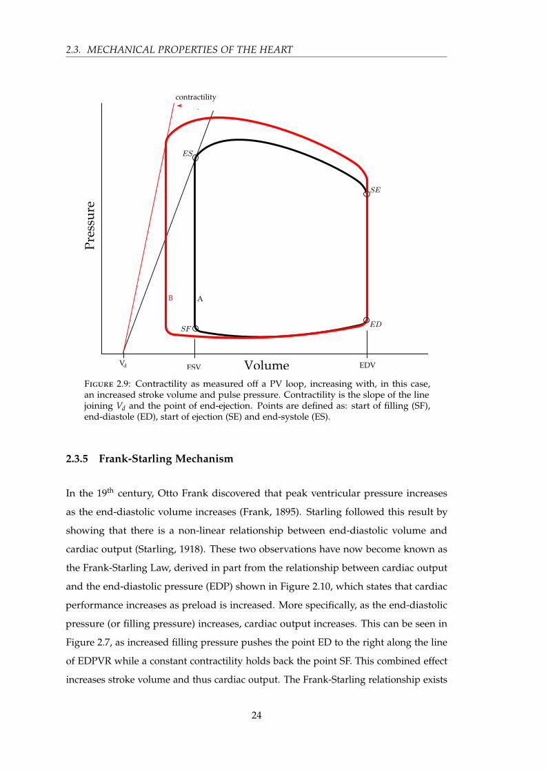
2.3. MECHANICAL PROPERTIES OF THE HEART
Figure 2.9: Contractility as measured off a PV loop, increasing with, in this case,an increased stroke volume and pulse pressure. Contractility is the slope of the linejoining Vd and the point of end-ejection. Points are defined as: start of filling (SF),end-diastole (ED), start of ejection (SE) and end-systole (ES).
2.3.5 Frank-Starling Mechanism
In the 19th century, Otto Frank discovered that peak ventricular pressure increases
as the end-diastolic volume increases (Frank, 1895). Starling followed this result by
showing that there is a non-linear relationship between end-diastolic volume and
cardiac output (Starling, 1918). These two observations have now become known as
the Frank-Starling Law, derived in part from the relationship between cardiac output
and the end-diastolic pressure (EDP) shown in Figure 2.10, which states that cardiac
performance increases as preload is increased. More specifically, as the end-diastolic
pressure (or filling pressure) increases, cardiac output increases. This can be seen in
Figure 2.7, as increased filling pressure pushes the point ED to the right along the line
of EDPVR while a constant contractility holds back the point SF. This combined effect
increases stroke volume and thus cardiac output. The Frank-Starling relationship exists
24
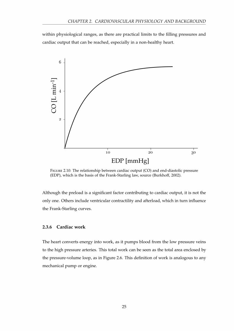
CHAPTER 2. CARDIOVASCULAR PHYSIOLOGY AND BACKGROUND
within physiological ranges, as there are practical limits to the filling pressures and
cardiac output that can be reached, especially in a non-healthy heart.
Figure 2.10: The relationship between cardiac output (CO) and end-diastolic pressure(EDP), which is the basis of the Frank-Starling law, source (Burkhoff, 2002).
Although the preload is a significant factor contributing to cardiac output, it is not the
only one. Others include ventricular contractility and afterload, which in turn influence
the Frank-Starling curves.
2.3.6 Cardiac work
The heart converts energy into work, as it pumps blood from the low pressure veins
to the high pressure arteries. This total work can be seen as the total area enclosed by
the pressure-volume loop, as in Figure 2.6. This definition of work is analogous to any
mechanical pump or engine.
25
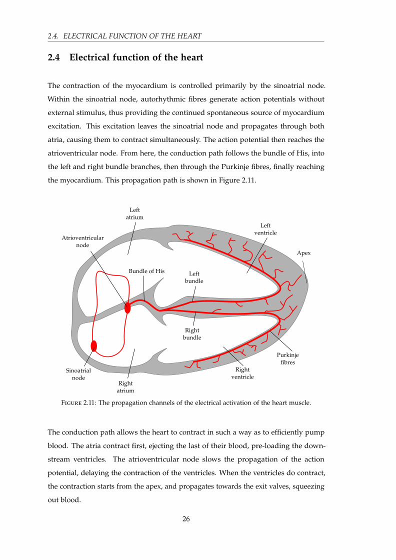
2.4. ELECTRICAL FUNCTION OF THE HEART
2.4 Electrical function of the heart
The contraction of the myocardium is controlled primarily by the sinoatrial node.
Within the sinoatrial node, autorhythmic fibres generate action potentials without
external stimulus, thus providing the continued spontaneous source of myocardium
excitation. This excitation leaves the sinoatrial node and propagates through both
atria, causing them to contract simultaneously. The action potential then reaches the
atrioventricular node. From here, the conduction path follows the bundle of His, into
the left and right bundle branches, then through the Purkinje fibres, finally reaching
the myocardium. This propagation path is shown in Figure 2.11.
Figure 2.11: The propagation channels of the electrical activation of the heart muscle.
The conduction path allows the heart to contract in such a way as to efficiently pump
blood. The atria contract first, ejecting the last of their blood, pre-loading the down-
stream ventricles. The atrioventricular node slows the propagation of the action
potential, delaying the contraction of the ventricles. When the ventricles do contract,
the contraction starts from the apex, and propagates towards the exit valves, squeezing
out blood.
26
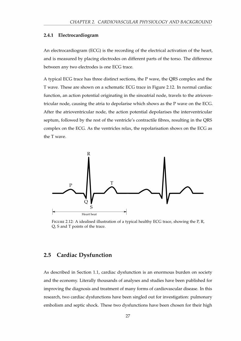
CHAPTER 2. CARDIOVASCULAR PHYSIOLOGY AND BACKGROUND
2.4.1 Electrocardiogram
An electrocardiogram (ECG) is the recording of the electrical activation of the heart,
and is measured by placing electrodes on different parts of the torso. The difference
between any two electrodes is one ECG trace.
A typical ECG trace has three distinct sections, the P wave, the QRS complex and the
T wave. These are shown on a schematic ECG trace in Figure 2.12. In normal cardiac
function, an action potential originating in the sinoatrial node, travels to the atrioven-
tricular node, causing the atria to depolarise which shows as the P wave on the ECG.
After the atrioventricular node, the action potential depolarises the interventricular
septum, followed by the rest of the ventricle’s contractile fibres, resulting in the QRS
complex on the ECG. As the ventricles relax, the repolarisation shows on the ECG as
the T wave.
Figure 2.12: A idealised illustration of a typical healthy ECG trace, showing the P, R,Q, S and T points of the trace.
2.5 Cardiac Dysfunction
As described in Section 1.1, cardiac dysfunction is an enormous burden on society
and the economy. Literally thousands of analyses and studies have been published for
improving the diagnosis and treatment of many forms of cardiovascular disease. In this
research, two cardiac dysfunctions have been singled out for investigation: pulmonary
embolism and septic shock. These two dysfunctions have been chosen for their high
27
2.5. CARDIAC DYSFUNCTION
prevalence in the ICU and the challenges they present to the ICU clinician in diagnosis
and treatment (Dombrovskiy et al., 2007; Bahloul et al., 2010).
2.5.1 Pulmonary Embolism
Pulmonary embolism (PE) is a cardiovascular emergency, and can lead to life-threatening,
but potentially reversible right ventricle failure. However, immediate diagnosis and
treatment is highly effective in reducing negative outcomes. Hence, the early diagnosis
of pulmonary embolism is critical (Torbicki et al., 2008). Over-treatment is also danger-
ous as it exposes the patient without PE to unjustified risk of major bleeding (Pineda
et al., 2001). Unfortunately, PE is not easy to diagnose, as clinical presentation is atypi-
cal (Al Otair et al., 2009). In an ICU, most patients require sedation and mechanical
ventilation, and therefore, the clinical manifestations expected from PE often cannot be
observed directly or immediately (Bahloul et al., 2010).
2.5.1.1 Physiology and clinical presentation of PE
Pulmonary embolism is the occlusion of the pulmonary bed, and most commonly
originates from deep venous thrombosis (DVT) of the legs (Tapson, 2008). PE ranges in
severity from asymptomatic, incidentally discovered emboli, to immediate death from
massive embolism. Pulmonary embolism becomes significant when more than 20–50 %
of the pulmonary bed is occluded (McIntyre and Sasahara, 1971), and the consequences
are mostly haemodynamic (Wood, 2002). Emboli can increase pulmonary vascular
resistance to a level which cannot be matched by the right ventricle. Alternatively,
systemic hypotension induced by PE, can lead to shock and acute right ventricle
failure. Left ventricular failure can also occur as a result of compromised cardiac
output from the rightward bulging interventricular septum (Jardin et al., 1997). Even
if right ventricular failure is initially survived, subsequent haemodynamic instability
may be caused by recurrent emboli, or a weakened right ventricular function, or other
pre-existing cardiovascular dysfunction. (Torbicki et al., 2008). Annually, more than
300,000 people in the United States die from acute PE (Tapson, 2007), and the diagnosis
is often not made until autopsy (Tapson, 2008; Investigators, 1997).
28

CHAPTER 2. CARDIOVASCULAR PHYSIOLOGY AND BACKGROUND
Both PE and DVT are clinical manifestations of venous thromboembolism (VTE), and
represent the spectrum of the one disease, VTE. In most cases, pulmonary embolism is
a consequence of DVT (Torbicki et al., 2008). For patients presenting with pulmonary
embolism, around 79 % have evidence of DVT, and for those that do not, it is likely that
the whole thrombus has already detached and embolized (Sandler and Martin, 1989;
Moser et al., 1994; Sevitt and Gallagher, 1961). Conversely, about half of the patients
presenting with DVT will have some form of pulmonary embolism as well (Tapson,
2008).
2.5.1.2 Diagnosis
Due to the non-specific nature of the clinical presentation of pulmonary embolism, a
range of tests and diagnostic strategies exists. The first and most important of these
assesses the probability of pulmonary embolism, based on the symptoms and signs
that are prevalent in PE. These symptoms and signs include breathing difficulties, chest
pain, low blood oxygen saturation, tachypnea and tachycardia (Torbicki et al., 2008),
palpitations, and pulmonary hypertension (Tapson, 2008).
Due to complications of sedation and mechanical ventilation, suspicion of pulmonary
embolism can be formed from un-explicated hypoxaemia and/or shock, and arterial
hypotension (Bahloul et al., 2010). Many systems exist that aim to indicate a probability
of pulmonary embolism based on clinical symptoms (Kearon, 2003; Wells et al., 2000;
Wicki et al., 2001; Wells et al., 1998; Perrier et al., 2000). However, none of these
methods allow the exclusion or confirmation of PE, but merely increase the index of its
suspicion (Torbicki et al., 2008). There are many further tests ranging in cost and level
of invasiveness, including ventilation-perfusion lung scan, D-dimer blood tests, helical
(or spiral) computed tomography (CT), echocardiography, and pulmonary angiography
(Kearon, 2003; Torbicki et al., 2008). However, these are limited by lack of sensitivity
and specificity, along with cost, time and expertise to perform and interpret.
Despite the limitations of clinical assessment, it still remains a critical first step in
the diagnosis of PE. Although most signs and symptoms have a poor combination
of sensitivity and specificity, when multiple variables are combined, it is possible to
achieve a good index of the probability of PE (Torbicki et al., 2008). Implicit clinical
judgement has also been shown to be valuable (Musset et al., 2002; Perrier et al., 2000,
29

2.5. CARDIAC DYSFUNCTION
1999), but is problematic in its lack of standardisation and teachability. The two most
used standardised rule sets for clinical assessment of PE are the Canadian Rule (Wells
et al., 2000), and the revised Geneva Rule (Le Gal et al., 2006).
A D-dimer test can refer to a number of similar blood assays that can effectively rule
out a PE diagnosis (Stein et al., 2004; Di Nisio et al., 2007). D-dimer levels are elevated
in plasma in the presence of an acute blood clot, and therefore a normal D-dimer result
means that acute PE or DVT is very unlikely (Torbicki et al., 2008). These tests range
from highly to moderately sensitive (Kearon, 2003).
Ventilation-perfusion scintigraphy (V/Q) scan is a safe and well understood scan that
can, for a normal result, eliminate the diagnosis of PE (Torbicki et al., 2008; Kruip et al.,
2003; Ten Wolde et al., 2004; Anderson, 2007). However, a V/Q scan is non-specific,
with only about one third of patients with V/Q scan defects actually having PE (Kearon,
2003; Groot et al., 1999; Miron et al., 1999). Hence, a V/Q scan has high sensitivity and
low specificity.
Helical computed tomography (CT), also known as spiral CT, is another widely used
clinical tool with good specificity and moderate sensitivity (Kearon, 2003). Traditional
computed tomography is not suitable for diagnoses of PE due to the long exposure
times that would be required. Helical CT can be completed during a breath hold,
or about 20 seconds. From two sets of studies, the sensitivity and specificity has
been shown to be around 70 % and 88 % respectively (Perrier et al., 2001; Monye and
Pattynama, 2001; Van Strijen et al., 2005).
Pulmonary angiography has historically been the standard for diagnosing PE (Kearon,
2003). However, it must be used with caution as it has side effects such as a small
chance or mortality (Kearon, 2003; Stein et al., 1992), as well as increasing the risk of
bleeding complications in some situations (Agnelli et al., 2002; Wan et al., 2004). It is
also technically demanding and costly. Furthermore, CT technology has improved to
the point where it can provide similar results in a non-invasive manner (Torbicki et al.,
2008).
Echocardiography is another test for diagnosing PE, and is particularly helpful in emer-
gency management situations (Torbicki et al., 2008). The main use of echocardiography
is for patients with shock or hypotension, and is used to rule out PE in the absence of
30
CHAPTER 2. CARDIOVASCULAR PHYSIOLOGY AND BACKGROUND
right ventricle (RV) overload or dysfunction. Echocardiography can visualise the right
heart haemodynamic changes (Goldhaber, 2002) along with a measure of RV volume
(Puchalski et al., 2007), which therefore means it can directly assess PE. However, it is
time consuming and costly and does not operate in real time.
The diagnosis of PE involves a nuanced approach that takes into account a variety
of variables and tests, using them to asses the probability of PE (Roy et al., 2006).
Better tests exist, but these are not readily assessed in real time. Hence, an implicit
diagnosis or noting of symptoms is required. What is necessary is an automated, higher
resolution measurement or diagnostic tool.
2.5.1.3 Treatment
With early diagnosis, treatment of PE is highly effective (Bahloul et al., 2010). The
initial treatment is aimed at the life-saving restoration of flow through the occluded
arteries, in combination with the prevention of early recurrences which can be fatal
(Torbicki et al., 2008). Haemodynamic and respiratory support are often necessary,
especially with patients presenting with shock or hypotension. Long term treatment
usually involves anticoagulation agents to prevent further recurrence (Tapson, 2008).
2.5.2 Septic Shock
Septic shock is an advanced stage of systemic inflammatory response syndrome (SIRS)
in the presence of an infection and organ failure (Annane et al., 2005). Septic shock
is a major cause of mortality and cost (Remick, 2007; Artero et al., 2012; Angus et al.,
2001), and continues to be a significant challenge to clinicians (Nduka and Parrillo,
2009; Dellinger et al., 2008).
2.5.2.1 Physiology and clinical presentation
Septic shock is a serious and life threatening disorder, that originates with a dysfunc-
tional immune system response to an infection and affects many aspects of the patient’s
physiology, importantly the cardiovascular system, and if left untreated, ultimately
leads to organ failure. Septic shock is thus a range or syndrome of related disorders
31
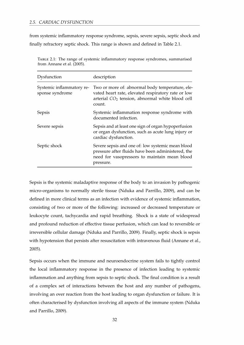
2.5. CARDIAC DYSFUNCTION
from systemic inflammatory response syndrome, sepsis, severe sepsis, septic shock and
finally refractory septic shock. This range is shown and defined in Table 2.1.
Table 2.1: The range of systemic inflammatory response syndromes, summarisedfrom Annane et al. (2005).
Dysfunction description
Systemic inflammatory re-sponse syndrome
Two or more of: abnormal body temperature, ele-vated heart rate, elevated respiratory rate or lowarterial CO2 tension, abnormal white blood cellcount.
Sepsis Systemic inflammation response syndrome withdocumented infection.
Severe sepsis Sepsis and at least one sign of organ hypoperfusionor organ dysfunction, such as acute lung injury orcardiac dysfunction.
Septic shock Severe sepsis and one of: low systemic mean bloodpressure after fluids have been administered, theneed for vasopressors to maintain mean bloodpressure.
Sepsis is the systemic maladaptive response of the body to an invasion by pathogenic
micro-organisms to normally sterile tissue (Nduka and Parrillo, 2009), and can be
defined in more clinical terms as an infection with evidence of systemic inflammation,
consisting of two or more of the following: increased or decreased temperature or
leukocyte count, tachycardia and rapid breathing. Shock is a state of widespread
and profound reduction of effective tissue perfusion, which can lead to reversible or
irreversible cellular damage (Nduka and Parrillo, 2009). Finally, septic shock is sepsis
with hypotension that persists after resuscitation with intravenous fluid (Annane et al.,
2005).
Sepsis occurs when the immune and neuroendocrine system fails to tightly control
the local inflammatory response in the presence of infection leading to systemic
inflammation and anything from sepsis to septic shock. The final condition is a result
of a complex set of interactions between the host and any number of pathogens,
involving an over reaction from the host leading to organ dysfunction or failure. It is
often characterised by dysfunction involving all aspects of the immune system (Nduka
and Parrillo, 2009).
32

CHAPTER 2. CARDIOVASCULAR PHYSIOLOGY AND BACKGROUND
The initial cause of sepsis comes primarily (80 %) from infections of the chest, abdomen,
genitourinary system and primary blood stream (Annane et al., 2003; Martin et al.,
2003; Alberti et al., 2002). The cardiovascular dysfunction resulting from septic shock
has been studied extensively over the last five decades (Calvin et al., 1981; Parker et al.,
1990; Munt et al., 1998; Poelaert et al., 1997). The results of these studies suggest that
cardiac performance during septic shock includes reduced left and right ventricular
ejection fractions, increased end-diastolic and end-systolic volumes of both ventricles
with normal stroke volume, while heart rate and cardiac output are elevated and
systemic vascular resistance is reduced.
2.5.2.2 Diagnosis
Due the complications of confirming — in a timely manner — both infection and organ
failure caused by infection, diagnosis can be difficult. To confirm a diagnosis of septic
shock there must be a recognised infection and an established causal link between
that infection and organ failure and shock (Annane et al., 2005). The infection may be
clinically obvious or otherwise discovered from recovery of pathogens from blood or
tissue culture. However, such cultures can take time to produce and are not usually
sensitive enough to rule out infection (Annane et al., 2005). Organ failure and the link
to infection can also be problematic to confirm, especially as organ failure scores often
ignore pre-existing organ function (Moreno et al., 2002). For cardiovascular failure, it
is important to differentiate between cardiac and circulatory dysfunction and is often
best characterised by echocardiography (Vieillard-Baron et al., 2003), which is resource
intensive, not real-time, and costly.
Shock is widely recognised in practice by the need for vasopressors to maintain arterial
pressure, (Bone et al., 1992). There are often indicators, such as low central venous
oxygen saturation (Rivers et al., 2001), visualisation of altered micro-circulation (Spronk
et al., 2002; De Backer et al., 2002), and impaired cardiovascular variability (Annane
et al., 1999). Hence, it can be diagnosed symptomatically, but only after it is advanced.
Due to the complications of confirming both infection and organ failure caused by
infection in a timely manner, diagnosis of septic shock can be difficult to diagnose with
certainty. To be confident of a septic shock diagnosis, a documented infection must
be present along with organ failure with no other relevant acute illness. Therefore, as
33

2.5. CARDIAC DYSFUNCTION
with many diagnostic methods, a probabilistic scale is used, with the likelihood of a
septic shock diagnosis reducing as the likelihood of infection decreases and other acute
illnesses are present. However, these diagnostics lack sensitivity and specificity, and
importantly, cannot be assessed in real-time or continuously.
2.5.2.3 Treatment
The main treatment strategies include immediate control of infection and haemo-
dynamic status, as well as support for failing organs, and restoration of immune,
neuroendocrine and haemostasis responses (Annane et al., 2005). Infection is primarily
controlled by appropriate antibodies. Management of shock and organ dysfunction can
be more involved, usually starting with fluid resuscitation and continuous monitoring
of central venous oxygen saturation, cardiac output among other cardiovascular metrics
(Annane et al., 2005). Anticoagulant therapies have also been shown to be an important
tool for treating septic shock (Rapaport et al., 1964; Corrigan et al., 1968). High-volume
haemofiltration can also be effective (Cole et al., 2001; Cornejo et al., 2006; Bouman,
2007; Rogiers, 2005), although it was first proposed as a renal replacement therapy
(Kramer et al., 1977). The ability to assess the impact of therapy, in real-time, would
greatly enhance the ability to treat patients effectively.
34

Chapter 3
Cardiovascular System Model
Throughout this research a lumped parameter model of the cardiovascular system is
used to describe cardiovascular and circulatory dynamics. This chapter describes the
model, as previously developed (Smith, 2004; Smith et al., 2004, 2005, 2006; Starfinger
et al., 2008a).
3.1 Introduction
Models are extremely useful constructions that can provide great insight into the
specific details of systems that cannot otherwise be known in a practical manner.
The cardiovascular system has many dynamics that would be clinically useful for
monitoring, diagnostics and treatment selection. However, many of them are too
invasive to measure directly. Hence, a cardiovascular model that can accurately capture
these properties and dynamics could have broad and significant use within a clinical
environment.
The cardiovascular model presented in this chapter has been previously published
(Smith, 2004; Smith et al., 2004, 2005, 2006; Starfinger et al., 2008a), and describes the
important properties and dynamics of the cardiovascular system under healthy and a
variety of pathological, physiological and clinical conditions (Revie et al., 2011a; Smith
et al., 2007, 2006; Starfinger et al., 2008a,b).
35
3.1. INTRODUCTION
3.1.1 The model
The model presented in this chapter is a lumped parameter model, and thus is a
compromise between accuracy and complexity. In this manner, a six chamber model is
presented that can represent the important dynamics without additional complexity.
An eight chamber version of this same model has also been published (e.g. Starfinger
et al., 2008a). However, it has yet to be shown that the added complexity of the
additional two chambers is beneficial in a clinical setting and is therefore not presented
in the research here.
The lumped nature of the model implies that the parameters and components of the
model relate metaphorically, rather than directly, to specific anatomy and physiology.
As such, each of the six chambers in the model represent the combination of a set
of general anatomical or physiological compartments. Another compromise is the
addition or exclusion of inertial effects, which, if included, moves the model from a
system of six differential equations to ten, adding significant computational expense to
solve the system, for, sometimes, minimal gain (Smith et al., 2003).
3.1.1.1 The six chambers
There are six distinct chambers in this model, each representing a portion of the
circulation with elastic properties. These compartments are, the left ventricle, the aorta,
the vena cava, the right ventricle, the pulmonary artery and the pulmonary vein. Four
of these chambers are passive and linear in their relationship between pressure and
volume. These passive chambers are, the aorta, the vena cava and the pulmonary
artery and vein. Due to the nature of the model each of these chambers represent the
summed effect of all the vessels within their respective section between the heart and
the capillaries.
The left and right ventricles are active chambers in the relationship between pressure
and volume, and, as such, have an elastance that varies with time in accordance with
the activation of the cardiac muscle. This time-varying elastance creates a non-linear
pressure-volume (PV) relationship. Therefore, active, non-linear PV relationship is the
basis of the rhythm and energetics of the model, and characterises each of the left and
36
CHAPTER 3. CARDIOVASCULAR SYSTEM MODEL
right ventricles as a pump. They are thus the primary elements driving circulatory
dynamics, as expected.
Due to the proximity of the ventricle chambers to each other, their activation is not
independent, but also not identical. This interaction is captured in the model by
coupling the two ventricles through the inter-ventricular septum and surrounding
pericardium. This enables the relationship between pressure and volume in each of the
ventricles to be partially independent and partially influenced by the other.
Since the heart and surrounding large vessels reside within the thoracic cavity, the
pressures in these vessels and compartments are also influenced by the thoracic pressure.
Including this thoracic pressure in the model enables the model to capture the effects
of respiration, whether natural or mechanical, and can play a significant role especially
in a critical care situation where both respiratory and cardiac support are required.
3.1.1.2 Inter-chamber properties
Between the chambers, there exist other properties to account for the remaining model
dynamics. These dynamics include pressure drops, inertial effects and valves. There
are four main circulatory valves, which appear at either side of the ventricles: the aortic,
tricuspid, pulmonary and mitral valves. These valves open on a positive pressure
gradient, and close on backward flow. Each valve causes a pressure drop and is thus
modelled alongside a resistance. Inertial effects can also be included here as the flow
and volume of blood is at its largest. Note that the model presented in this chapter
is presented with and without inertia, as the addition of inertia greatly increases the
computation cost of simulation.
There are two other important pressure drops represented in the model, occurring
across the pulmonary and systemic portions of the circulation. These pressure drops are
modelled as the summed resistance over the entire left (systemic) and right (pulmonary)
sides of the circulation. Therefore, they include all the resistance to flow through the
artery, capillaries and veins on their respective side.
37
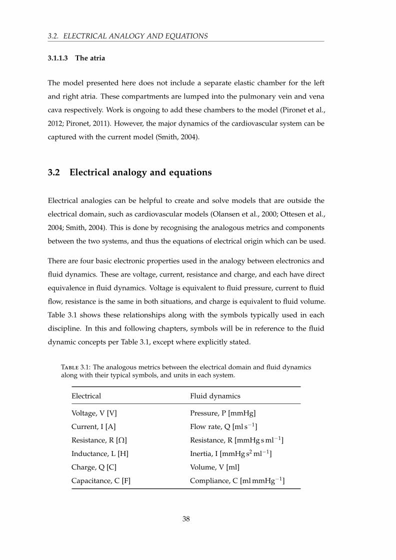
3.2. ELECTRICAL ANALOGY AND EQUATIONS
3.1.1.3 The atria
The model presented here does not include a separate elastic chamber for the left
and right atria. These compartments are lumped into the pulmonary vein and vena
cava respectively. Work is ongoing to add these chambers to the model (Pironet et al.,
2012; Pironet, 2011). However, the major dynamics of the cardiovascular system can be
captured with the current model (Smith, 2004).
3.2 Electrical analogy and equations
Electrical analogies can be helpful to create and solve models that are outside the
electrical domain, such as cardiovascular models (Olansen et al., 2000; Ottesen et al.,
2004; Smith, 2004). This is done by recognising the analogous metrics and components
between the two systems, and thus the equations of electrical origin which can be used.
There are four basic electronic properties used in the analogy between electronics and
fluid dynamics. These are voltage, current, resistance and charge, and each have direct
equivalence in fluid dynamics. Voltage is equivalent to fluid pressure, current to fluid
flow, resistance is the same in both situations, and charge is equivalent to fluid volume.
Table 3.1 shows these relationships along with the symbols typically used in each
discipline. In this and following chapters, symbols will be in reference to the fluid
dynamic concepts per Table 3.1, except where explicitly stated.
Table 3.1: The analogous metrics between the electrical domain and fluid dynamicsalong with their typical symbols, and units in each system.
Electrical Fluid dynamics
Voltage, V [V] Pressure, P [mmHg]
Current, I [A] Flow rate, Q [ml s−1]
Resistance, R [Ω] Resistance, R [mmHg s ml−1]
Inductance, L [H] Inertia, I [mmHg s2 ml−1]
Charge, Q [C] Volume, V [ml]
Capacitance, C [F] Compliance, C [ml mmHg−1]
38

CHAPTER 3. CARDIOVASCULAR SYSTEM MODEL
There are three main electrical circuit components with analogous fluid dynamic
properties. These components are: the resistor, representing the resistance of a pipe or
vessel to the flow of fluid; the inductor, representing the inertia of the fluid; and the
capacitor, which represents the ability of a compartment to hold and release a volume
of fluid. These components and their equivalents are shown with their respective
symbols and base units in Table 3.2.
Table 3.2: The analogous components between the electrical domain and fluid dynam-ics along with their typical symbols.
Electrical Fluid dynamics metaphor
Resistor ( ) Vessel resistance
Inductor ( ) Fluid inertia
Capacitor ( ) Vessel compliance
From the analogy in Tables 3.1–3.2, many fluid dynamic systems can be modelled as
electrical circuits and solved using the established circuit theory and equations. There
are three equations used, Ohm’s law, and the relationship between current and voltage
for both capacitor and an inductor. Ohm’s law provides an equation to relate fluid
pressure to resistance and flow, and is defined:
P = Q× R (3.1)
The equation governing a capacitor, and therefore vessel compliance is defined:
Q = C · dPdt
(3.2)
From Equation (3.2), the relationship between pressure, volume and elastance (units of
mmHg ml−1) can be derived:
Q =1E· dP
dt(3.3)
⇒ dPdt
= E ·Q (3.4)
⇒ P = E ·∫
Qdt (3.5)
⇒ P = E ·V (3.6)
39

3.3. MODEL BACKGROUND
Finally, the equation governing an inductor, and therefore fluid inertia is defined:
P = L · dQdt
(3.7)
Variables are as defined in Tables 3.1–3.2.
3.3 Model background
3.3.1 Windkessel model
The Windkessel model was first described by the German physiologist by Frank (1899),
and since then has been used in numerous physiological models to simulate the
elasticity of a compartment. The term Windkessel loosely translates from German as
“air chamber”. The original model was based on a hydraulic circuit consisting of a
water pump connected to a chamber of air. As water is pumped into the chamber,
the water compresses the air at the same time as pushing water out of the chamber
and back to the pump. The compressibility of the air simulates the compliance of
the chamber. This type of model is most commonly used to simulate blood in a
vessel that exhibits elasticity of its walls, typically referred to by its inverse value,
compliance = 1/elastance.
There are many different ways to formulate a Windkessel model, from a simple two-
element model to higher order models, both in parallel and in series. The CVS model
presented in the chapter is largely based on a chain of three-element series models, one
of which is shown as an electrical analogy in Figure 3.1, where the capacitor represents
compliance (C), the resistance (R) represents resistance to blood flow back to the pump,
and the inductance (I) represents the inertia of the blood.
3.4 Schematic model derivation
The general principle behind a lumped parameter model is to achieve a description of
the necessary system properties and dynamics with the minimal amount of complexity,
lumping any excess complexity into single parameters or units. In this manner the
40

CHAPTER 3. CARDIOVASCULAR SYSTEM MODEL
Figure 3.1: A Windkessel model and a three-element series electrical representation.This is the basic compartment or element model from which the overall CVS model isderived.
circulation can be traced through its complete cycle, forming a closed loop fluid
dynamic system. Each significant section (by volume) of the circulation is represented
as an elastic chamber (Windkessel model) which is allowed to vary in pressure and
volume with a constant chamber stiffness.
Each passage of flow will encounter resistance, and the portions that have highest mass
and volume will also exhibit the greatest inertia. Ignoring the valves in the veins, there
are four main valves in the normal human circulation which are located either side of
the ventricles. Finally, the pumping of the heart is modelled in the elastic chambers,
representing the ventricles, by allowing these chambers to vary in elastance over time,
to capture the heart’s active, electro-mechanical activation. Hence, this time-varying
elastance is the core mechanism by which the model is pressurised and driven, and can
thus be thought of as the driver function. The full schematic representation is shown in
Figure 3.2, along with an analogous electrical circuit.
41
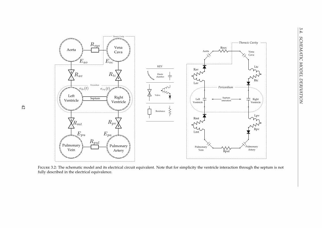
3.4.SC
HEM
ATIC
MO
DEL
DER
IVATIO
N
Figure 3.2: The schematic model and its electrical circuit equivalent. Note that for simplicity the ventricle interaction through the septum is notfully described in the electrical equivalence.
42
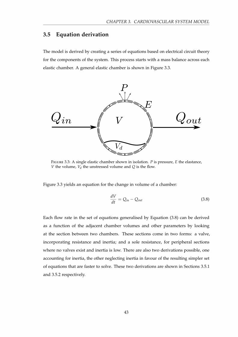
CHAPTER 3. CARDIOVASCULAR SYSTEM MODEL
3.5 Equation derivation
The model is derived by creating a series of equations based on electrical circuit theory
for the components of the system. This process starts with a mass balance across each
elastic chamber. A general elastic chamber is shown in Figure 3.3.
Figure 3.3: A single elastic chamber shown in isolation. P is pressure, E the elastance,V the volume, Vd the unstressed volume and Q is the flow.
Figure 3.3 yields an equation for the change in volume of a chamber:
dVdt
= Qin −Qout (3.8)
Each flow rate in the set of equations generalised by Equation (3.8) can be derived
as a function of the adjacent chamber volumes and other parameters by looking
at the section between two chambers. These sections come in two forms: a valve,
incorporating resistance and inertia; and a sole resistance, for peripheral sections
where no valves exist and inertia is low. There are also two derivations possible, one
accounting for inertia, the other neglecting inertia in favour of the resulting simpler set
of equations that are faster to solve. These two derivations are shown in Sections 3.5.1
and 3.5.2 respectively.
43

3.5. EQUATION DERIVATION
3.5.1 The valves
There are four sections that have valves, representing the four valves found in the heart:
the aortic valve, the tricuspid valve, the pulmonary valve, and the mitral value. Each of
these valves can be represented by a resistor, inductor and diode, shown in Figure 3.4.
As the diode is only meant to represent a fluid dynamic construction of no back flow,
the physical details of an electrical diode, such as forward and reverse bias, are ignored.
Figure 3.4: The representation of a valve between two chambers. The valve is modelledas a diode, with resistance and inertial effects.
Using electrical equations for the voltage, or pressure difference across this section,
P2 − P1, a differential equation in Q can be derived from Equations (3.1) and (3.7):
P2 − P1 = Q · R +.
Q · L (3.9)
⇒.
Q =P2 − P1 −Q · R
L(3.10)
To account for the diode/valve, a Heaviside function is introduced to zero all negative
flow. The Heaviside is defined:
H( f ) =
0 if f ≤ 0
1 if f = 0(3.11)
44

CHAPTER 3. CARDIOVASCULAR SYSTEM MODEL
Thus the diode is implemented as H ( f ), and is defined:
H ( f ) = H( f ) · f (3.12)
3.5.2 Peripheral flow
The model also has inter-chamber flow through the systemic and pulmonary circulation
with no valves and negligible inertia. This situation is shown in Figure 3.5. This case
results in the following equations:
P2 − P1 = Q · R (3.13)
⇒ Q =P2 − P1
R(3.14)
Figure 3.5: Flow between elastic chambers with only resistance.
3.5.3 Pressure and volume
At this point, there are six equations relating the change in a chamber’s volume to its
pressure and surrounding parameters of resistance and inductance. For the four passive
chambers of the model in Figure 3.2, the pressure can be found as a function of volume
through the electrical equations of a capacitor outlined with Equations (3.3)–(3.6),
resulting in:
P = E ·V (3.15)
It is now necessary to formulate the pressure, as a function of volume, for the driven
chambers representing the two ventricles.
45

3.5. EQUATION DERIVATION
3.5.4 Ventricle pressure and volume
The relationship between pressure and volume in the ventricles is more complicated
than Equation (3.15), as these chambers are actively pressurising and de-pressurising
over time, and thus the pressure-volume relationship is non-linear. A common method
for describing this relationship is to allow the elastance in the model components
for the ventricular chambers to vary with time, thus giving the name time-varying
elastance (Beyar et al., 1987; Burkhoff and Tyberg, 1993; Chung et al., 1997; Santamore
and Burkhoff, 1991).
From Figure 3.6, it can be seen that limits for the elastance in the ventricular chambers
are defined by the two relationships of ESPVR and EDPVR as the upper and lower
bounds respectively. These two elastance relationships are described in Section 2.3. To
use these limits, descriptive equations are required and these equations are defined for
the linear ESPVR:
Pes = Ees (Ves −Vd) (3.16)
For the non-linear EDPVR they are defined:
Ped = P0
(eλ(Ved−V0) − 1
)(3.17)
where the subscripts es and ed represent end-systole and end-diastole respectively, and
the parameters P0, λ and V0 represent the gradient, curvature and volume at zero
pressure respectively for EDPVR.
To define the complete relationship for pressure and volume in the ventricles the
time-varying elastance is normalised to vary between 0 (at end-diastole) and 1 (at
end-systole), and given the symbolic notation of e(t). This normalised curve can then
be used as a weighted sum to provide the pressure-volume relationship outside the
already defined points of end-diastole and end-systole. Ventricular pressure is thus
defined as:
P = e (t) · Pes + (1− e (t)) · Ped (3.18)
Since the volume is now allowed to vary beyond that at end-diastole and end-systole,
and noting that the ventricles reside within the pericardium, the full pressure-volume
46
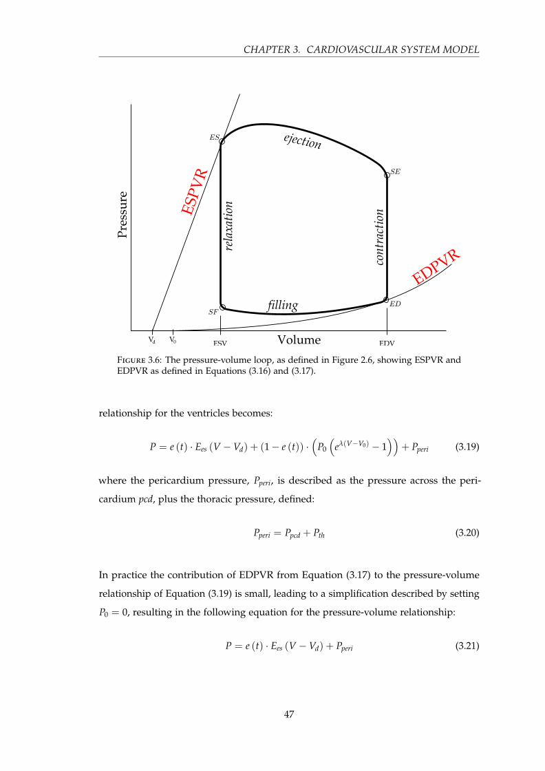
CHAPTER 3. CARDIOVASCULAR SYSTEM MODEL
Figure 3.6: The pressure-volume loop, as defined in Figure 2.6, showing ESPVR andEDPVR as defined in Equations (3.16) and (3.17).
relationship for the ventricles becomes:
P = e (t) · Ees (V −Vd) + (1− e (t)) ·(
P0
(eλ(V−V0) − 1
))+ Pperi (3.19)
where the pericardium pressure, Pperi, is described as the pressure across the peri-
cardium pcd, plus the thoracic pressure, defined:
Pperi = Ppcd + Pth (3.20)
In practice the contribution of EDPVR from Equation (3.17) to the pressure-volume
relationship of Equation (3.19) is small, leading to a simplification described by setting
P0 = 0, resulting in the following equation for the pressure-volume relationship:
P = e (t) · Ees (V −Vd) + Pperi (3.21)
47

3.5. EQUATION DERIVATION
This equation closely resembles the general equation for a passive chamber in Equa-
tion (3.15), with an additional pressure, which under certain conditions can be assumed
to be negligible. Although the full unsimplified ventricular pressure-volume relation-
ship is used in the simulation of the model, the simplified version is used in this
research as a means to calculate and estimate the time-varying elastance e(t).
At this point in the derivation, six differential equations have been defined for the
volume of each elastic chamber in the model. However, unlike the four passive
chambers, the volumes and pressures in the driven chambers do not stand in isolation,
but rather interact with one another, requiring more complexity to the driven chamber
pressure-volume equations.
3.5.5 Ventricular interaction
The two ventricles of the heart share a common muscle boundary called the inter-
ventricular septum. The ventricles also reside within the pericardium. This shared wall
and surrounding membrane gives rise to shared dynamics and interaction between the
two ventricles. These shared dynamics play an important role in the overall dynamics
of the cardiovascular system (Weber et al., 1982; Fogel et al., 1998), and account for
differences between the two ventricles in terms of pressure and volume that otherwise
could not be captured. This aspect is especially important in abnormal pathologies,
such as an overloaded right ventricle with pulmonary hypertension, which results in
impaired left ventricle filling due to ventricular interaction (Gan et al., 2006). In such
cases, the right ventricle extends into the normally larger left ventricle, skewing the
balance of pressure and volume normally seen between these chambers. Hence, the
model must be able to capture this dynamic, and does so via this model mechanism.
Figure 3.7 shows two depictions of the two ventricles and their interaction in volume
and pressure. For ease of modelling, the concept of a ‘free wall volume’ is defined as
the volume contained by the boundary of the wall. This free wall volume is distinct
from a normal volume as shown in Figure 3.7, as well as creating imaginary volumes
such as the volume of the septum Vspt.
Given the concept of a free wall compartment, designated by appending f to an existing
subscript, the ventricular volumes can be defined in relation to the free wall volumes
48

CHAPTER 3. CARDIOVASCULAR SYSTEM MODEL
Figure 3.7: The free wall concept, top graphic, showing the left and right free wallvolumes along with the septum free wall volume. The actual pressure and volume ofthe ventricles and surroundings are shown in the lower graphic.
and the septum volume:
Vlv = Vlvf + Vspt (3.22)
Vrv = Vrvf −Vspt (3.23)
49
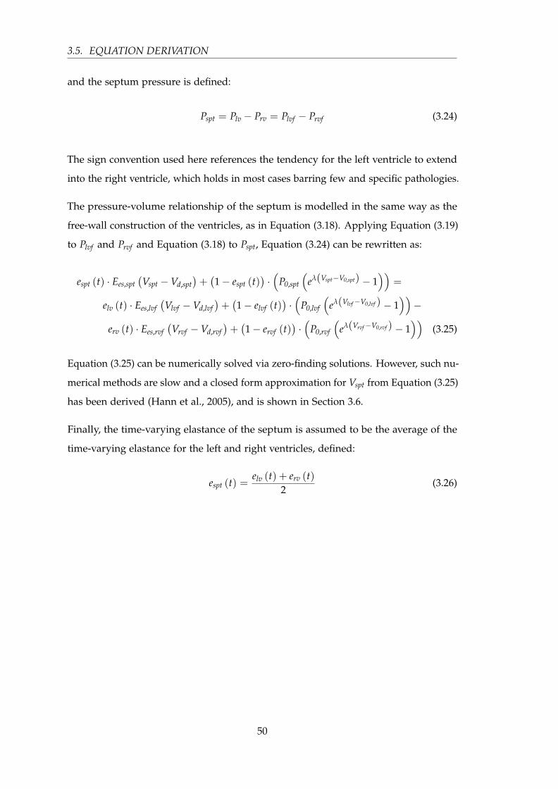
3.5. EQUATION DERIVATION
and the septum pressure is defined:
Pspt = Plv − Prv = Plvf − Prvf (3.24)
The sign convention used here references the tendency for the left ventricle to extend
into the right ventricle, which holds in most cases barring few and specific pathologies.
The pressure-volume relationship of the septum is modelled in the same way as the
free-wall construction of the ventricles, as in Equation (3.18). Applying Equation (3.19)
to Plvf and Prvf and Equation (3.18) to Pspt, Equation (3.24) can be rewritten as:
espt (t) · Ees,spt(Vspt −Vd,spt
)+(1− espt (t)
)·(
P0,spt
(eλ(Vspt−V0,spt) − 1
))=
elv (t) · Ees,lvf(Vlvf −Vd,lvf
)+(1− elvf (t)
)·(
P0,lvf
(eλ(Vlvf−V0,lvf ) − 1
))−
erv (t) · Ees,rvf(Vrvf −Vd,rvf
)+(1− ervf (t)
)·(
P0,rvf
(eλ(Vrvf−V0,rvf ) − 1
))(3.25)
Equation (3.25) can be numerically solved via zero-finding solutions. However, such nu-
merical methods are slow and a closed form approximation for Vspt from Equation (3.25)
has been derived (Hann et al., 2005), and is shown in Section 3.6.
Finally, the time-varying elastance of the septum is assumed to be the average of the
time-varying elastance for the left and right ventricles, defined:
espt (t) =elv (t) + erv (t)
2(3.26)
50
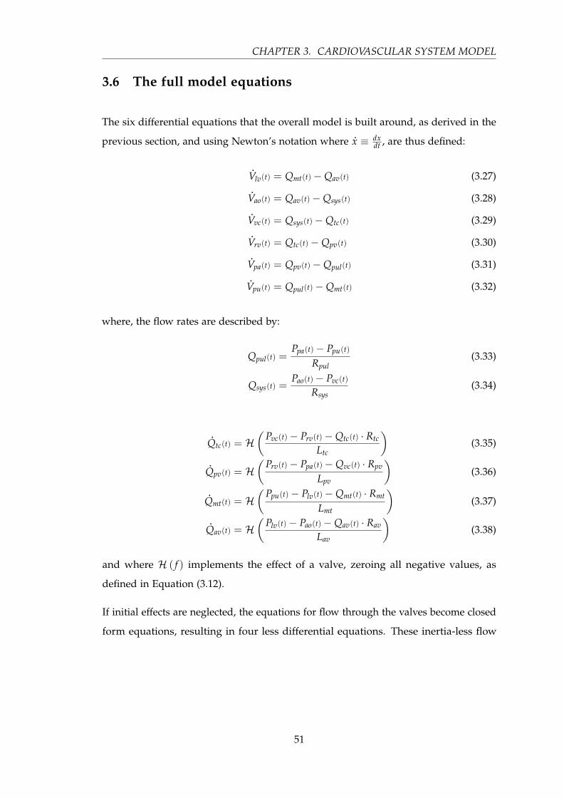
CHAPTER 3. CARDIOVASCULAR SYSTEM MODEL
3.6 The full model equations
The six differential equations that the overall model is built around, as derived in the
previous section, and using Newton’s notation where .x ≡ dxdt , are thus defined:
.Vlv(t) = Qmt(t)−Qav(t) (3.27).
Vao(t) = Qav(t)−Qsys(t) (3.28).
Vvc(t) = Qsys(t)−Qtc(t) (3.29).
Vrv(t) = Qtc(t)−Qpv(t) (3.30).
Vpa(t) = Qpv(t)−Qpul(t) (3.31).
Vpu(t) = Qpul(t)−Qmt(t) (3.32)
where, the flow rates are described by:
Qpul(t) =Ppa(t)− Ppu(t)
Rpul(3.33)
Qsys(t) =Pao(t)− Pvc(t)
Rsys(3.34)
.Qtc(t) = H
(Pvc(t)− Prv(t)−Qtc(t) · Rtc
Ltc
)(3.35)
.Qpv(t) = H
(Prv(t)− Ppa(t)−Qvc(t) · Rpv
Lpv
)(3.36)
.Qmt(t) = H
(Ppu(t)− Plv(t)−Qmt(t) · Rmt
Lmt
)(3.37)
.Qav(t) = H
(Plv(t)− Pao(t)−Qav(t) · Rav
Lav
)(3.38)
and where H ( f ) implements the effect of a valve, zeroing all negative values, as
defined in Equation (3.12).
If initial effects are neglected, the equations for flow through the valves become closed
form equations, resulting in four less differential equations. These inertia-less flow
51
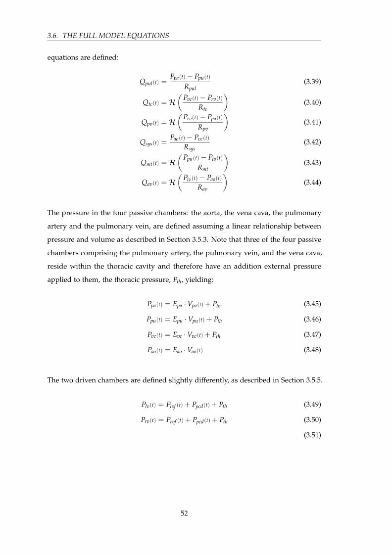
3.6. THE FULL MODEL EQUATIONS
equations are defined:
Qpul(t) =Ppa(t)− Ppu(t)
Rpul(3.39)
Qtc(t) = H(
Pvc(t)− Prv(t)
Rtc
)(3.40)
Qpv(t) = H(
Prv(t)− Ppa(t)
Rpv
)(3.41)
Qsys(t) =Pao(t)− Pvc(t)
Rsys(3.42)
Qmt(t) = H(
Ppu(t)− Plv(t)
Rmt
)(3.43)
Qav(t) = H(
Plv(t)− Pao(t)
Rav
)(3.44)
The pressure in the four passive chambers: the aorta, the vena cava, the pulmonary
artery and the pulmonary vein, are defined assuming a linear relationship between
pressure and volume as described in Section 3.5.3. Note that three of the four passive
chambers comprising the pulmonary artery, the pulmonary vein, and the vena cava,
reside within the thoracic cavity and therefore have an addition external pressure
applied to them, the thoracic pressure, Pth, yielding:
Ppa(t) = Epa ·Vpa(t)+ Pth (3.45)
Ppu(t) = Epu ·Vpu(t)+ Pth (3.46)
Pvc(t) = Evc ·Vvc(t)+ Pth (3.47)
Pao(t) = Eao ·Vao(t) (3.48)
The two driven chambers are defined slightly differently, as described in Section 3.5.5.
Plv(t) = Plvf (t)+ Ppcd(t)+ Pth (3.49)
Prv(t) = Prvf (t)+ Ppcd(t)+ Pth (3.50)
(3.51)
52

CHAPTER 3. CARDIOVASCULAR SYSTEM MODEL
where
Plvf (t) = elv(t) · Ees,lv ·(Vlvf (t)−Vd,lvf
)+
(1− elv(t)) · P0,lvf ·(
eλlvf (Vlvf (t)−V0,lvf ) − 1)
(3.52)
and
Prvf (t) = erv(t) · Ees,rv ·(Vrvf (t)−Vd,rvf
)+
(1− erv(t)) · P0,rvf ·(
eλrvf (Vrvf (t)−V0,rvf ) − 1)
(3.53)
and
Ppcd(t) = P0,pcd ·(
eλpcd·(Vpcd(t)−V0,pcd) − 1)
(3.54)
The free wall ventricle volumes are defined:
Vlvf (t) = Vlv(t)−Vspt(t) (3.55)
Vrvf (t) = Vrv(t)+ Vspt(t) (3.56)
and when summed, the ventricles make the volume of the pericardium, defined:
Vpcd(t) = Vlv(t)+ Vrv(t) (3.57)
The volume of the septum is defined as a closed-form approximation to Equation (3.25),
as derived (Hann et al., 2005):
Vspt =ab
(3.58)
53
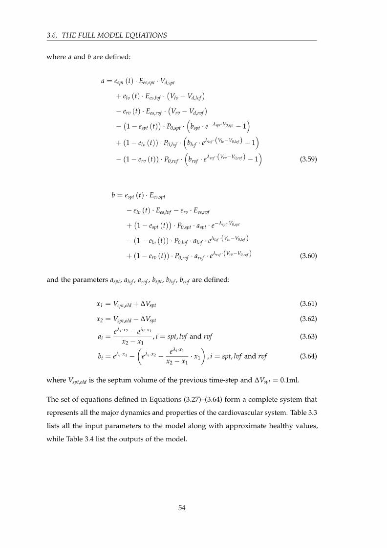
3.6. THE FULL MODEL EQUATIONS
where a and b are defined:
a = espt (t) · Ees,spt ·Vd,spt
+ elv (t) · Ees,lvf ·(Vlv −Vd,lvf
)− erv (t) · Ees,rvf ·
(Vrv −Vd,rvf
)−(1− espt (t)
)· P0,spt ·
(bspt · e−λspt·V0,spt − 1
)+ (1− elv (t)) · P0,lvf ·
(blvf · eλlvf ·(Vlv−V0,lvf ) − 1
)− (1− erv (t)) · P0,rvf ·
(brvf · eλrvf ·(Vrv−V0,rvf ) − 1
)(3.59)
b = espt (t) · Ees,spt
− elv (t) · Ees,lvf − erv · Ees,rvf
+(1− espt (t)
)· P0,spt · aspt · e−λspt·V0,spt
− (1− elv (t)) · P0,lvf · alvf · eλlvf ·(Vlv−V0,lvf )
+ (1− erv (t)) · P0,rvf · arvf · eλrvf ·(Vrv−V0,rvf ) (3.60)
and the parameters aspt, alvf , arvf , bspt, blvf , brvf are defined:
x1 = Vspt,old + ∆Vspt (3.61)
x2 = Vspt,old − ∆Vspt (3.62)
ai =eλi ·x2 − eλi ·x1
x2 − x1, i = spt, lvf and rvf (3.63)
bi = eλi ·x1 −(
eλi ·x2 − eλi ·x1
x2 − x1· x1
), i = spt, lvf and rvf (3.64)
where Vspt,old is the septum volume of the previous time-step and ∆Vspt = 0.1ml.
The set of equations defined in Equations (3.27)–(3.64) form a complete system that
represents all the major dynamics and properties of the cardiovascular system. Table 3.3
lists all the input parameters to the model along with approximate healthy values,
while Table 3.4 list the outputs of the model.
54

CHAPTER 3. CARDIOVASCULAR SYSTEM MODEL
Table 3.3: Model input parameters for the six-chamber cardiovascular model alongwith units and healthy values.
Input Name Units Value
Rpul Pulmonary vascular resistance mmHg s ml−1 0.018
Rsys Systemic vascular resistance mmHg s ml−1 1.0889
Rtc Tricuspid valve resistance mmHg s ml−1 0.0237
Rpv Pulmonary valve resistance mmHg s ml−1 0.0055
Rmt Mitral valve resistance mmHg s ml−1 0.0158
Rav Aortic valve resistance mmHg s ml−1 0.018
Ltc Tricuspid valve blood inertia mmHg s2 ml−1 8.0093× 10⁻⁵
Lpv Pulmonary valve blood inertia mmHg s2 ml−1 1.4868× 10⁻⁴
Lmt Mitral valve blood inertia mmHg s2 ml−1 7.6968× 10⁻⁵
Lav Aortic valve blood inertia mmHg s2 ml−1 1.2189× 10⁻⁴
Epa Pulmonary artery elastance mmHg ml−1 0.369
Epu Pulmonary vein elastance mmHg ml−1 0.0073
Evc Vena cava elastance mmHg ml−1 0.0059
Eao Aortic elastance mmHg ml−1 0.6913
Pth Thoracic pressure mmHg −4
Ees,lv Left ventricle end-systolic elastance mmHg ml−1 2.8798
Vd,lvf Unstressed left ventricle volume ml 0
V0,lvf Zero-pressure left ventricle volume ml 0
P0,lvf Zero-volume left ventricle pressure mmHg 0.1203
λlvf Left ventricle lambda ml−1 0.033
Ees,rv Right ventricle end-systolic elastance mmHg ml−1 0.5850
Vd,rvf Unstressed right ventricle volume ml 0
V0,rvf Zero-pressure right ventricle volume ml 0
P0,rvf Zero-volume right ventricle pressure mmHg 0.2157
λrvf Right ventricle lambda ml−1 0.023
55

3.7. SIMULATION
Table 3.3 — (continued)
Input Name Units Value
Ees,spt Septum end-systolic elastance mmHg ml−1 48.0754
Vd,spt Unstressed septum volume ml 2
V0,spt Zero-pressure septum volume ml 2
P0,spt Zero-volume septum pressure mmHg 1.1101
λspt Septum lambda ml−1 0.435
P0,pcd Zero-volume pericardium pressure mmHg 0.5003
V0,pcd Zero-pressure pericardium volume ml 200
λpcd Pericardium lambda ml−1 0.03
3.7 Simulation
The solution to the CVS model is found by solving the system of differential equa-
tions listed in Equations (3.27)–(3.32) and, if inertia is not neglected, additionally
Equations (3.35)–(3.38). In this research, the routine ODE45 from the software package
MATLAB R© (The MathWorks, Natick, USA) is used to numerically solve for the state
variables defined:
x = [Vlv, Vao, Vvc, Vrv, Vpa, Vpu, Qtc, Qpv, Qmt, Qav] (3.65)
or, if inertia is neglected, the state variables defined:
x = [Vlv, Vao, Vvc, Vrv, Vpa, Vpu] (3.66)
Apart from these parameters the simulation needs some extra information. The first is
an initial state, which is a vector corresponding to Equation (3.65) or Equation (3.66).
56
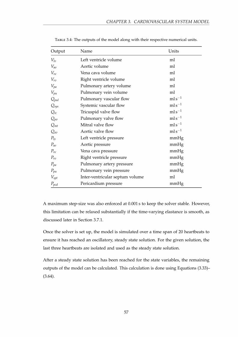
CHAPTER 3. CARDIOVASCULAR SYSTEM MODEL
Table 3.4: The outputs of the model along with their respective numerical units.
Output Name Units
Vlv Left ventricle volume mlVao Aortic volume mlVvc Vena cava volume mlVrv Right ventricle volume mlVpa Pulmonary artery volume mlVpu Pulmonary vein volume mlQpul Pulmonary vascular flow ml s−1
Qsys Systemic vascular flow ml s−1
Qtc Tricuspid valve flow ml s−1
Qpv Pulmonary valve flow ml s−1
Qmt Mitral valve flow ml s−1
Qav Aortic valve flow ml s−1
Plv Left ventricle pressure mmHgPao Aortic pressure mmHgPvc Vena cava pressure mmHgPrv Right ventricle pressure mmHgPpa Pulmonary artery pressure mmHgPpu Pulmonary vein pressure mmHgVspt Inter-ventricular septum volume mlPpcd Pericardium pressure mmHg
A maximum step-size was also enforced at 0.001 s to keep the solver stable. However,
this limitation can be relaxed substantially if the time-varying elastance is smooth, as
discussed later in Section 3.7.1.
Once the solver is set up, the model is simulated over a time span of 20 heartbeats to
ensure it has reached an oscillatory, steady state solution. For the given solution, the
last three heartbeats are isolated and used as the steady state solution.
After a steady state solution has been reached for the state variables, the remaining
outputs of the model can be calculated. This calculation is done using Equations (3.33)–
(3.64).
57

3.7. SIMULATION
3.7.1 Parameters
To simulate this model, all parameters must be defined, which includes the left and
right driver functions, or time-varying elastance. This definition of the driver function
has been done in several ways in the past. The most accurate method of creating a
function for the time-varying elastance is to measure it directly. Direct measurement is
done by re-arranging Equation (3.19), such that:
e (t) =P + Pperi − Ped
Ees (V −Vd)− Ped(3.67)
where Ped is the lower bound, as defined Equation (3.17) and repeated here:
Ped = P0
(eλ(V−V0) − 1
)(3.68)
In most cases, including this research, where the ventricle pressure and volume are
measured, measurements are done with an open chest and thus Pperi = 0 by definition.
It can also be assumed that Ped is small in comparison to Ees and therefore neglected.
These assumptions are discussed further in Section 3.8. This approach leaves the
time-varying elastance defined as a function of the ventricle pressure and volume:
e (t) =P
Ees ·V(3.69)
where
Ees = max(
PV
)(3.70)
However, this approach in Equations (3.67)–(3.70) requires the invasive measurement of
pressure and volume in the left and right ventricles, which ultimately goes against the
overall ethic of the model’s clinical application, which is to avoid further invasiveness.
There have been several approaches to address this problem and these are discussed in
Chapter 4.
These approaches, although removing the need for invasive measurement of the
ventricles, also removed much of the patient-specific energetic information present in
the time-varying elastance. Hence, a patient-specific approach has been developed
and published (Stevenson et al., 2012a,b), and is presented in Chapters 6 and 7. This
58

CHAPTER 3. CARDIOVASCULAR SYSTEM MODEL
patient-specific approach creates an estimation for the time-varying elastance as defined
in Equation (3.69).
3.7.2 Simulation example
An example simulation using healthy porcine data is given in Figure 3.8. This simula-
tion was done using a measured time-varying elastance and a thoracic pressure of zero,
Pth = 0. The goal is to show the basic simulation and resulting model outputs.
Figure 3.8: A single heart beat from a simulation of the model. The parameters werechosen to resemble a healthy porcine subject, with a measured time-varying elastance.Pressure in the ventricle and downstream vessel are shown for each side of the heart,including the ventricle volume.
3.8 Discussion
The model presented in this chapter is a lumped parameter model. As such, it does not
relate exactly to physiology. Assumptions and simplifications were made to achieve a
balance of complexity and accuracy.
59

3.8. DISCUSSION
3.8.1 Simplifications
Perhaps the biggest simplification is the representation of large sections of the circu-
lation through discrete model chambers. These chambers appear, and are named, in
the model as a single section, but physiologically and anatomically represent a much
wider context. For example the aortic chamber represents the entire series of elastic
arteries of the systemic circulation. Therefore, the associated model parameters are
averages or averaged representations of this large section of the circulation.
Another simplification in this model is the lack of distinct chambers representing the
atria. In general, the atria have only a small influence on the cardiovascular trends, and
as such, the additional complexity required was considered unjustified. However, the
effects of the atria are partially present in the current model, as they are lumped into
the pulmonary vein and vena cava chambers. Work is ongoing in formulating the atria
as separate identifiable chambers (Pironet et al., 2012; Pironet, 2011).
3.8.2 Assumptions
At a fluid dynamics level, there are a few assumptions made in the derivation of the
model. To make the transition from fluid dynamics to electrical circuits, fluid flow
was modelled assuming a Poiseuille profile. A Poiseuille flow profile represents an
incompressible, Newtonian, laminar, fully developed flow through a rigid vessel of
constant circular cross-section. To assume Poiseuille flow implies assumptions about
the nature of blood and its containing vessels:
• Blood can be treated as incompressible (White, 1991).
• Blood is assumed to behave as a Newtonian fluid with constant viscosity (Fung,
1993). This cannot be said for flow in the capillaries but is reasonable in the larger
vessels.
• Blood vessels are assumed to be rigid with a constant cross-sectional area. This is
consistent with a Windkessel model where the combination of a rigid pipe and an
elastic chamber capture the fluid dynamics and vessel compliance (Tsitlik et al.,
1992; Melchior et al., 1992).
60
CHAPTER 3. CARDIOVASCULAR SYSTEM MODEL
• Laminar, uni-directional, axi-symmetric flow is assumed throughout the circu-
lation. Some turbulence will occur in places around the circulation, especially
in proximity to the valves and bifurcations. However, this is assumed to be of
negligible significance to the overall flow profile.
• The flow is assumed to be fully developed, and thus the velocity profile is constant
along the length of the vessel (Fung, 1993).
These assumptions allow the formulation of a fluid dynamic system as a simple
electrical circuit (Beyar et al., 1987; Burkhoff and Tyberg, 1993; Chung et al., 1997;
Olansen et al., 2000; Smith et al., 2004), as shown in Section 3.2. However, these
assumptions are all simplifications and approximations of the real situation and thus,
to varying degrees, add error into the model. This is inherent to the nature of a
minimally complex model, and thus cannot be avoided. Rather, error is minimised by
making only justifiable and reasonable assumptions.
One of the more significant assumptions is that the flow is fully developed. Due
to the pulsatile nature of blood flow in the larger vessels of the circulation, this is
obviously false in these regions. Inertial effects, if included in the simulation with
Equations (3.35)–(3.38), can compensate for this approximation. However, the effect of
inertia can generally be regarded as insignificant, which is typically the case in many
models.
The main parameters of the model, namely, elastance (E), resistance (R), and inductance
(L) are assumed to be constant except for the ventricular elastances which vary in
time. This assumption is a simplification of the real physiology. However, it does
not introduce much error compared to measurement errors, and vastly reduces the
complexity and computational cost for solving the model. Hence, the assumption of
constant parameter values is common among lumped parameter models (Beyar et al.,
1987; Olansen et al., 2000; Ursino, 1999; Wang et al., 2003).
As already mentioned, the effects of inertia are small. Therefore, the benefit of adding
a time-dependency to the inertial parameters makes little sense. This set of parameters
is also based mostly on the properties of the blood, whose changes are too slow to be
captured by a single simulation of the model.
61

3.8. DISCUSSION
The parameter of resistance comes in two forms, valve resistance (Rav, Rtc, Rpv and Rmt),
and peripheral resistance (Rsys and Rpul). Valve resistance has been suggested to be the
most useful clinical index of valve function, as it represents more closely the functional
impairment of the valve, than other indices such as valve area (Antonini-Canterin et al.,
1999). Valve resistance has also been shown to be less dependant on flow (Antonini-
Canterin et al., 1999; Ford et al., 1994; Casale et al., 1992; Blitz and Herrmann, 1996;
Bermejo et al., 1996; Ford et al., 1990), although these findings have been questioned
(Blais et al., 2001; Mascherbauer et al., 2004). Valve resistance is also easily combined
with other haemodynamic calculations (Ford et al., 1994). Peripheral resistance can
reasonably be assumed to be constant, as the flow and pressure through the capillaries
is relatively steady over a single heartbeat.
The third constant parameter, elastance, must also be divided between venous and
arterial elastance. For the venous system, the elastance has been shown to be constant
over physiological ranges of venous pressure (Batzel and Bachar, 2010). Assuming
arterial elastance to be constant is the largest simplification of all the parameters, as
the aorta, in some capacity, actively pushes blood in a similar, though much weaker,
manner to the ventricles, and it is widely accepted that the arterial elastance is non-
linear with respect to pressure (Batzel and Bachar, 2010; Li et al., 1990; Westerhof et al.,
2009). However, the effect of modelling this variable and patient- and condition-specific
non-linearity has been shown to be of no measurable advantage in different Windkessel
models (Fogliardi et al., 1996). Therefore, a constant arterial elastance can be justified.
3.8.3 Limitations
The lumped parameter nature of the model gives rise to some limitations on the
accuracy and detail of the physiological dynamics that the model can capture. For
example, the dicrotic notch in the aortic pressure waveform is not captured by the
model, due to the lack of reflected pressure waveforms in the model. However, the
model does capture all the major dynamics of the cardiovascular system that are
important in managing and controlling cardiac dysfunction in a clinical setting.
The valves are modelled based on an ‘open on pressure, close on flow’ formulation, and
inherently do not allow flow in the reverse direction. Therefore dysfunctions such as
mitral (Paeme et al., 2011) and aortic regurgitation, which are the insufficient valvular
62

CHAPTER 3. CARDIOVASCULAR SYSTEM MODEL
functions allowing some back flow, cannot be captured without modification to the
model.
Other limitations arise from the assumptions made in the derivation of the model as
discussed in Section 3.8.2.
3.9 Summary
This chapter has presented a lumped parameter cardiovascular model that is capable of
representing the important properties and dynamics of the cardiovascular system in a
healthy state as well as a range of pathological conditions. The model is a compromise
between physiological accuracy and computational expense, and has been shown in
two configurations, one accounting for inertia, the other neglecting inertial effects.
The model contains six elastic chambers representing portions of the circulatory system,
two of which act as pumps. Resistances, inertial effects and valves are all included
to capture the important dynamics of the cardiovascular system. Inter-ventricular
coupling is also captured through the interaction of the two ventricular chambers, as
well as the pressure effects from the respiratory system.
This model is the basis for the work done in the remaining chapters of this research.
63

Chapter 4
CVS Model Identification
Before the CVS model can be of clinical use, the model parameters must be identified
to a specific patient’s cardiovascular state using physiologically and clinically relevant
model parameter values. This process, of parameter identification that matches the
outputs of the model to measurements that are commonly available in a clinical setting,
is presented in this chapter.
4.1 Introduction
This chapter presents a method for the identification of the parameters of the six-
chamber model presented in Chapter 3, and shown here for clarity in Figure 4.1.
This process results in a model whose outputs match a set of measured clinical data,
and accurately represents the dynamics of the cardiovascular system from which the
measurements were taken. Therefore, the identified model has potential for patient-
specific diagnostic and treatment processes in a clinical environment.
To be useful in a clinical setting, the identification process must use only measurements
that are generally available in the ICU. It should also be able to provide real-time
feedback as well as additional and useful cardiovascular information that can be readily
understood and used by clinical staff. Thus, the identified model should aggregate the
measured data into a clear, physiological picture.
65

4.1. INTRODUCTION
Figure 4.1: The full six-chamber model of the cardiovascular system as outlined inChapter 3.
The identification algorithm presented in this chapter was based on a previously
developed integral-based method (Starfinger, 2008; Starfinger et al., 2008b,a, 2007),
and presented in more detail by Revie et al. (2011b). The previous method relied on
knowledge of the left and right ventricular pressure and volume waveforms, limiting
the real-time clinical usage of the model. The method presented here removes the
dependency on ventricular waveforms, and thus uses only measurements commonly
available in the ICU. These changes clear the way for the model’s use in clinical
applications. The measurements used include the aortic, pulmonary artery and central
venous pressures, stroke volume, cardiac output, global end-diastolic volume, heart
66

CHAPTER 4. CVS MODEL IDENTIFICATION
rate and the timing of the mitral and tricuspid valve closures.
4.2 Pre-requisites
4.2.1 Identification Assumptions
As with the model itself, assumptions must be made to identify the model given
the limited set of data that can be used in the identification process. This choice is
an intentional limitation. However, because of how they are chosen, none of these
assumptions are of great significance.
4.2.1.1 Steady state
The measured data is assumed to be at steady state. This choice allows for the further
assumption that the left and right stroke volumes are equal. Assuming stroke volume
equality is physiologically reasonable, because the heart generally maintains a balance
of ejected blood as described by the Frank Starling mechanism.
4.2.1.2 Inertia is negligible
For simplicity, inertia in the model is neglected. This choice has very little impact on
the output of the model (Smith et al., 2004), and significantly decreases the complexity
of the model and the computational cost of simulation. Thus, it reduces the number of
parameters to identify, and the computational cost of identification.
4.2.1.3 Valve timing
It is assumed that at the time the ventricle inlet valves close, the ventricle pressure is
equal to the pressure directly upstream. This choice translates into:
Plv(tmt) ≡ Ppu (tmt) (4.1)
Prv(ttc) ≡ Pvc (ttc) (4.2)
67
4.2. PRE-REQUISITES
This assumption makes sense for this model because the model neglects both atria
(Smith et al., 2004; Starfinger et al., 2007). Hence, the pulmonary vein effectively
connects directly to the ventricle, and, similarly, for the right side. Since inertia
has been neglected, the valves close on a negative pressure gradient, as opposed to
backward flow when inertia is included. Therefore, the mitral valve will close when
the left ventricle pressure first increases above the pulmonary vein, which occurs
momentarily after Plv = Ppu in the model.
4.2.1.4 Change in contractilities are proportional
To identify the contractilities of the left and right ventricles with the standard set of
measurements in the ICU environment, some assumptions need to be made to give
the required additional information. It is thus assumed that any inotropic effect acts
equally to change cardiac contractility on both sides of the heart, resulting in the ratio
of contractilities staying constant over time. This assumption enables the identification
of the separate left and right ventricle contractilities in an ICU setting.
4.2.1.5 GEDV ∝ LVEDV + RVEDV
It is assumed that the global end-diastolic volume (GEDV) is proportional to the sum
of the ventricle end-diastolic volumes. The GEDV that is measured in the ICU setting,
which is usually found from thermodilution, would include the volume of the atria
as well. However, this volume is minimal, as most of the atrial volume will have been
ejected into the ventricles by the time of end-systole. Therefore, the major contributors
to GEDV are the left ventricle end-diastolic volume (LVEDV) and the right ventricle
end-diastolic volume (RVEDV) (Sakka et al., 2000), and thus the assumption made is
reasonable for the way this value is used.
4.2.1.6 Valve resistances
It is assumed that the resistance of the valves does not change over short periods of
time, which is physiologically reasonable. This assumption allows the identification
of the model to run over several beats and eliminates spurious, non-clinically relevant
variables.
68
CHAPTER 4. CVS MODEL IDENTIFICATION
4.2.1.7 Unidentified parameters
There are several parameters of the full model that have assumed values and are not
identified. These variables include:
• V0,lv = V0,rv = V0,ao = V0,pa = V0,vc = V0,pa = 0
• Vd,lvf = Vd,rvf = 23 for swine (Desaive et al., 2008), and 0 for humans
• P0,lvf = P0,rvf = 0
The reason these parameters are left at the assumed values defined, is the lack of specific
information from a typical ICU setting. This choice also results in the model focusing
more on the physiologically and clinically important model parameters, ensuring they
are identified in an accurate and robust manner relative to these assumptions.
4.2.2 Measured data in the ICU
As stated, the measurements on which the identification of the model is based, are
restricted to those that can be readily accessed in a typical ICU setting. The mea-
surements required include: arterial pressure (AP), central venous pressure (CVP),
pulmonary artery pressure (PAP), heart rate (HR) mitral valve timing (tmt), cardiac
output (CO) and global end-diastolic volume (GEDV).
4.2.2.1 Arterial pressure
The actual measurement required by the model is aortic pressure (Pao). However, the
exact pressure is not usually available in the ICU. Instead, aortic pressure can be found
from radial arterial pressure, which is normally available through one of several known
methods (Westerhof et al., 2008; O’Rourke, 2004; Hope et al., 2004; Cloud et al., 2003;
Pauca et al., 2001; Chen et al., 1997).
4.2.2.2 Pulmonary artery pressure
Pulmonary artery pressure, Ppa, as measured with a pulmonary artery catheter (PAC),
is decreasingly common in a general ICU bed. However, it can be measured and is still
69

4.3. IDENTIFICATION PROCESS
common practice in some ICUs. This is more common in specialised ICUs such as the
cardiac ICU.
4.2.2.3 Central venous pressure (CVP)
Central venous pressure (CVP) is commonly available in the ICU as standard practice
through a central line catheter. This pressure is then equivalent to the modelled vena
cava pressure (Pvc).
4.2.2.4 Cardiac output and GEDV
Both cardiac output and global end-diastolic volume can be measured through ther-
modilution techniques (Michard et al., 2003; Sakka et al., 2000; Stetz et al., 1982; Ganz
et al., 1971), which are commonly used in an ICU setting.
4.2.2.5 Heart rate
Electrocardiogram (ECG) is also a matter of standard practice in the ICU, and easily
provides the heart rate and period, along with an estimate of the timing of the mitral
and tricuspid valve closures.
4.3 Identification process
The identification process uses two key conceptual methods. First, the model is reduced
in size and complexity to a point where individual parameters can be identified. These
simplified models are then put back together to estimate the remaining parameters.
This method greatly increases the robustness of the identification process. Second,
each parameter is identified using a proportional feedback control approach to match a
specific output measurement.
The whole process is inherently iterative. Initial values are established. Each sub-model
is then run, updating the respective parameters. The ventricular contractility is then
updated, after which the sub-models are put back together and the full six-chamber
70

CHAPTER 4. CVS MODEL IDENTIFICATION
model is run, to update the remaining two elastance parameters. In each successive
update the parameters get closer to their true value. After all parameter values have
settled, an identified solution is said to have been found.
4.3.1 Simplified models
The six-chamber model described in Chapter 3 is divided into two sub-models, one for
the systemic circulation, the other for the pulmonary circulation. Each sub-model can
stand on its own, but can also feed parameters to the other side during the iterative
identification process. Each simplified model gets run in two steps. Each step identifies
a subset of the parameters of that model. More detail about each of the models can
be found in Sections 4.4.2 and 4.4.3. Both sub-models, systemic and pulmonary, are
shown in Figure 4.2 in the context of the full six-chamber model, showing how the
six-chamber model is broken up, and the communication between the two sub-models.
4.3.2 Proportional gain identification
Proportional gain is a robust and fast way to identify a parameter given that two
assumptions apply. First, the parameter in question must be either directly or inversely
proportional to a unique known measurement. This measurement becomes the surro-
gate error metric for the parameter, and thus must be related to its respective parameter.
Second, each output metric can be used as a surrogate error by only one parameter.
Once a parameter has been linked with its own measurement, the ratio of the measured
value to the modelled value (or its inverse) can be used to correct the current parameter
value. In other words, the parameter is multiplied by a number proportional to its
surrogate error. This approach is defined:
Pn+1 =AB· Pn (4.3)
where Pn is a parameter at iteration n, and the ratio of A to B is the ratio of the
measured to modelled output metric or its inverse, depending on the relationship
between the measured metric and the parameter. As A and B converge, Pn+1 → Pn.
71
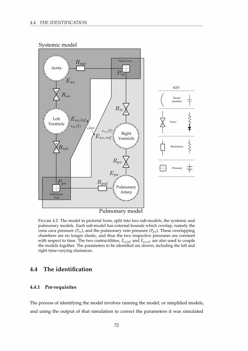
4.4. THE IDENTIFICATION
Figure 4.2: The model in pictorial form, split into two sub-models, the systemic andpulmonary models. Each sub-model has external bounds which overlap, namely thevena cava pressure (Pvc), and the pulmonary vein pressure (Ppu). These overlappingchambers are no longer elastic, and thus the two respective pressures are constantwith respect to time. The two contractilities, Ees,lvf and Ees,rvf are also used to couplethe models together. The parameters to be identified are shown, including the left andright time-varying elastances.
4.4 The identification
4.4.1 Pre-requisites
The process of identifying the model involves running the model, or simplified models,
and using the output of that simulation to correct the parameters it was simulated
72

CHAPTER 4. CVS MODEL IDENTIFICATION
with. This approach means an initial simulation must be run with initial values for
the parameters and input functions. Aside from parameters with assumed values, as
defined in Section 4.2.1, the default parameter values are listed in Table 4.1.
The time-varying elastance (TVE) for the left, elv(t), and right, erv(t), ventricles must also
be defined, as both simplified models require this input function. Due to the centrality
of these functions to model output, it is critical that the time-varying elastance be known
accurately. Every step of the identification process, except for the contractility, uses a
model simulation involving one or both of these ventricular time-varying elastances.
Therefore, any error in these functions will affect the whole process in a complex and
undefined manner. This issue is discussed further in Section 4.5.
In particular, this need for accurate time-varying elastances was part of the motivation
behind the development of algorithms that would accurately estimate the left and right
time-varying elastances from available ICU metrics (Stevenson et al., 2012a,b). These
algorithms are presented in Chapters 6 and 7.
Table 4.1: The parameters of the six-chamber model along with their initial values,surrogate errors and the sub-model in which they are used.
Parameter Initialvalue
Surrogate error Sub model
Rmt 0.05 left stroke volume systemic (set 1)
Rsys 2.5 mean Pao systemic (set 1)
Eao 2.5 Pao pulse pressure systemic (set 1)
Rav 0.04 max(
ddt (Pao)
)systemic (set 2)
Rtc 0.04 right stroke volume pulmonary (set 1)
Rpul 0.4 mean Ppa pulmonary (set 1)
Epa 2.1 Ppa pulse pressure pulmonary (set 1)
Rpv 0.03 max(
ddt
(Ppa))
pulmonary (set 2)
Ees,lvf 2 – ventricle
Ees,rvf 0.8 – ventricle
Pvc 5 – pulmonary & systemic
Ppu 5 – pulmonary & systemic
73

4.4. THE IDENTIFICATION
4.4.2 Systemic sub-model identification
The systemic model is a little less than half of the full model, taking the systemic side
of the circulation between the pulmonary vein and the vena cava. However, the two
end points, the pulmonary vein and the vena cava, are no longer elastic chambers, but
have constant pressures with respect to time. Thus, they become pseudo parameters
for the sub-models. Ppu is identified by the systemic model, while Pvc is identified by
the pulmonary model. Therefore, the systemic model is now a two-chamber model.
The first step in the identification process is to simulate this two-chamber systemic
model with the required parameters from Table 4.1. The results of the simulation
include, by definition, the surrogate errors associated with the model parameters. Thus,
the sub-model parameters can be adjusted accordingly.
There are three points of iteration. First, the systemic ID set 1 is solved, followed by the
systemic ID set 2. Since the parameters that are updated in set 2 affect the values of
those updated in set 1, the whole process is repeated until all parameters are changed
by less than 0.5 %. This process is illustrated in Figure 4.3
Figure 4.3: The identification of the systemic model with three points of iteration.The model is given seven parameter values and the time-varying elastance of the leftventricle, and returns five modified, and converged, parameter values.
4.4.2.1 Systemic ID iteration set 1: Rmt, Rsys, and Eao
The first set of iterations focuses on the three sub-model parameters, Rmt, Rsys, and Eao.
All three are simultaneously adjusted after each simulation, while keeping all other
74

CHAPTER 4. CVS MODEL IDENTIFICATION
parameters constant. Once these values have converged to within 0.5 % this iteration
set is said to have converged and the identification process moves on to the systemic
ID set 2.
These three parameters were controlled at the end of each iteration by the following
proportional control, defined:
Rmt n+1 =SVlv, modelled
SVmeasured· Rmt n (4.4)
Rsys n+1 =Pao, measured
Pao, modelled· Rsys n (4.5)
Eao n+1 =PPao, measured
PPao, modelled· Eao n (4.6)
4.4.2.2 Systemic ID iteration set 2: Rav, and Ppu
The next step in the identification process is to find values for Rav, and Ppu. Both
parameters depend on correct values from the previous iteration set, and thus are
identified separately. The pulmonary vein pressure is assumed equal to the left
ventricular pressure at the time the mitral valve closes. This assumption is reasonable
given that when the mitral valve closes, isolating the ventricle from the pulmonary
vein, the flow rate is zero and thus there should be no pressure drop across the valve.
This point in time is defined:
Ppu = Plv(tmt) (4.7)
As the pulmonary vein pressure is found as a function of the left ventricle pressure, it
can be seen that the value of Rmt is required, as ultimately, the left ventricle pressure is
a function of Rmt (see Section 3.6).
Rav must also be separated from the initial set, as its identification requires the correct
stroke volume to be present. The adjustment to Rav is thus defined:
Rav n+1 =max
(ddt (Pao, modelled)
)max
(ddt (Pao, meassured)
) · Rav n (4.8)
75

4.4. THE IDENTIFICATION
4.4.3 Pulmonary sub-model identification
The pulmonary sub-model is the pulmonary equivalent of the systemic model, taking
the other ‘half’ of the full model. In the same fashion as the systemic model, the two
overlapping chambers — the vena cava and pulmonary vein — have constant pressures
with respect to time. Pvc becomes a pseudo-parameter in the pulmonary model, while
Ppu is taken as already identified by the systemic model, and thus held constant.
In an analogous process to the systemic model, the pulmonary model is broken into
two parts to identify two different sets of parameters, and a similar iteration process
takes place, as shown in Figure 4.4.
Figure 4.4: The identification of the pulmonary model with three points of iteration.The model is given seven parameter values and the time-varying elastance of the rightventricle, and returns five modified, and converged, parameter values.
4.4.3.1 Pulmonary ID iteration set 1: Rtc, Rpul and Epa
In an equivalent manner to the systemic ID iteration set 1, two resistances and an
elastance are identified simultaneously by the following proportional control, defined:
Rtc n+1 =SVrv, modelled
SVmeasured· Rtc n (4.9)
Rpul n+1 =Ppa, measured
Ppa, modelled· Rpul n (4.10)
Epa n+1 =PPpa, measured
PPpa, modelled· Epa n (4.11)
76
CHAPTER 4. CVS MODEL IDENTIFICATION
4.4.3.2 Pulmonary ID iteration set 2: Rpv and Pvc
Once iteration set 1 has converged, the remaining resistance Rpv and pseudo-parameter
Pvc can be found. Similar to the pulmonary vein pressure, the vena cava pressure is
assumed to be equal to the right ventricle pressure at the time the tricuspid valve closes.
Hence, it is defined:
Pvc = Prv (ttc) (4.12)
The pulmonary valve resistance proportional control is then defined:
Rvc n+1 =max
(ddt
(Ppa, modelled
))max
(ddt
(Ppa, meassured
)) · Rvc n (4.13)
4.4.4 Ventricle contractility
Ventricular contractility was identified in two steps. First, the sum of the left and right
ventricular contractility, Ees, sum, was identified using GEDV as a surrogate error metric.
GEDV can be measured through a thermodilution test, and modelled as the sum of
the maximum volumes of the left and right ventricles. The proportional control is thus
defined:
Ees, sum n+1 =GEDVmodelled
GEDVmeasured· Ees, sum n (4.14)
Second, the individual contractilities were split from the sum using a ratio of elastances
that stays constant for each subject. This assumption requires that inotropic effects
act equally on both sides of the heart. The ratio of contractilities is found through a
correlation with the ratio of afterloads and modelled vena cava pressure (Anrep, 1912;
Knowlton and Starling, 1912; Sarnoff and Mitchell, 1961), and is defined:
CE =Pao − Pvc
Pao − Ppa=
Ees, lvf
Ees, lvf + Ees, rvf= constant (4.15)
where a bar represents the mean.
The value of CE is assumed to stay constant for each subject and is thus calculated
as an average over a range of data for each subject, neglecting physiological outliers,
CE < 0.6, ensuring that the left ventricle has a greater contractility than the right
77

4.4. THE IDENTIFICATION
(Hosepud and Greenberg, 2007; Konstam et al., 1985). Using the subjects CE, the left
and right contractilities can be calculated from Ees, sum as defined:
Ees, lvf = CE · Ees, sum (4.16)
Ees, rvf = Ees, sum − Ees, lvf (4.17)
Once the contractilities are updated, the identification can start from the beginning
with the newly found values, potentially producing different maximum values for the
left and right ventricular volumes, resulting in a different modelled GEDV. Thus, the
iterative process continues until GEDV stabilises.
The six-chamber model includes more detailed ventricular interaction through the
modelling of the ventricular septum, as shown in Figures 4.1 and 4.5. The systemic and
pulmonary sub-models can also include this interaction, by the inclusion of non-zero
values for Vspt and Ppcd. With identified values for the left and right ventricular con-
tractility, values for Vspt and Ppcd can also be updated, as described by Equations (3.54)
and (3.58).
4.4.5 Venous chambers
After the systemic and pulmonary sub-models have been identified and the ventricle
contractility has been found, the only remaining parameters to the full six-chamber
model are the elastance of the vena cava, Evc, and pulmonary vein, Epu, chambers.
These two elastances, Evc and Epu, are identified using a five-chamber model, under
the same proportional control method as the rest of the parameters. This five-chamber
model is the full six-chamber model with the pulmonary vein pressure held constant
at the value identified with the simplified models, and is shown in Figure 4.5.
Evc is identified by matching the vena cava pressure output of the five-chamber model
to that which was identified in the systemic model. Thus, Pvc becomes a surrogate error
metric for Evc. This proportional control is defined:
Evc n+1 =Pvc sm
mean(
Pvc fm
) · Evc n (4.18)
where sm donates the systemic model and fm, the five chamber model.
78

CHAPTER 4. CVS MODEL IDENTIFICATION
Figure 4.5: The modified version of the model that is used to identify the venouschamber elastances. This model is identical to the full six-chamber except for oneaspect, the pulmonary vein pressure is held constant, turning the six-chamber modelinto a five chamber model.
This process is iterated until Evc converges, after which the value of Epu can be directly
calculated. This approach is a result of a dependence of the pulmonary volume, Vpu
on Evc. Specifically, after Evc has settled to the correct value, Epu can be calculated
from the constant pulmonary vein pressure and the pulmonary vein volume, using the
relationship defined:
Epu =Ppu sm
mean(
Vpu fm
) (4.19)
79

4.5. TIME-VARYING ELASTANCE (TVE)
4.4.6 Valve Resistance
Inter-beat variability in measured data can be a major problem in identification al-
gorithms. This variability is a significant problem with this algorithm for the valve
resistances, which are highly sensitive to small changes in the measured data. To
reduce the sensitivity, the model was identified over a range of different measured
beats, and, for each set, the valve resistances were stored and averaged. The whole
identification process is then re-run, leaving out the identification of the now known
and averaged resistances values.
Furthermore, the equations for Ppu and Pvc as functions of their respective ventricle
pressures were replaced with proportional control, thus removing the dependence on
the valve timing. This proportional control is defined:
Ppu n+1 =SVlv, modelled
SVmeasured· Ppu n (4.20)
Pvc n+1 =SVrv, modelled
SVmeasured· Pvc n (4.21)
4.4.7 Parameter bounds
To make the identification process more robust and physiologically meaningful, each
parameter was constrained within bounds appropriate for that parameter. This con-
straining of values increases the stability of the model edge cases, and also ensures that
the identified parameters have physiological relevance. These parameter bounds are
listed in Table 4.2.
4.5 Time-varying elastance (TVE)
The time-varying elastance is a central part of the six-chamber model that is presented
in Chapter 3 and identified in the current chapter. Physiologically, the time-varying
elastance represents the activation of the myocardial muscle, and is intrinsically linked
with the energetics of the heart (Suga, 1990b). In both the model and physiological
context, the time-varying elastance is a key component of much of the cardiovascular
dynamics, in value, timing and shape. This function is what drives the model. Therefore,
80

CHAPTER 4. CVS MODEL IDENTIFICATION
Table 4.2: The allowable range of values for the parameters of the six-chamber model.Each parameter is restricted in the identification to be within this range, to insure theparameters are physiologically meaningful.
Parameter Allowed parameter range
Rmt 0.005 – 0.5
Rsys 0.1 – 10
Eao 0.1 – 10
Rav 0.005 – 0.5
Rtc 0.005 – 0.5
Rpul 0.05 – 10
Epa 0.1 – 10
Rpv 0.005 – 0.5
Ees,lvf 0.1 – 10
Ees,rvf 0.1 – 10
Pvc 0.1 – minimum of 15 and (min (Pao, measured)− 2)
Ppu 1 – minimum of 15 and(min
(Ppa, measured
)− 2)
it is critical to get an accurate representation of the time-varying elastance to get
meaningful results from the model and the identified parameters. More detail and
physiological context about the time-varying elastance is given in Chapter 5.
There are two important effects of time-varying elastance on the six-chamber model,
which occur in simulation and identification. As already stated, simulation of the
model requires accurate time-varying elastances. However, the identification process
also relies heavily on these functions. In every step, except the identification of the
contractility, the model (or a simplified version of the model) is simulated. This use of
simulation only compounds the sensitivity of the model to the time-varying elastance,
as the parameters along with the model simulation are functions of the time-varying
elastance.
The interactions between the time-varying elastance and the modelled outputs for any
simulation are too complex to attempt to quantify. This issue becomes more problematic
when the identification process is included. However, what can be shown is that the
81
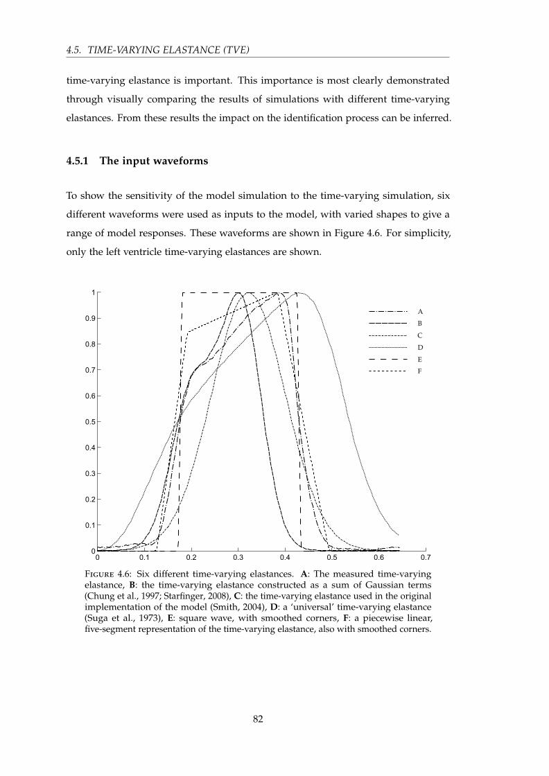
4.5. TIME-VARYING ELASTANCE (TVE)
time-varying elastance is important. This importance is most clearly demonstrated
through visually comparing the results of simulations with different time-varying
elastances. From these results the impact on the identification process can be inferred.
4.5.1 The input waveforms
To show the sensitivity of the model simulation to the time-varying simulation, six
different waveforms were used as inputs to the model, with varied shapes to give a
range of model responses. These waveforms are shown in Figure 4.6. For simplicity,
only the left ventricle time-varying elastances are shown.
Figure 4.6: Six different time-varying elastances. A: The measured time-varyingelastance, B: the time-varying elastance constructed as a sum of Gaussian terms(Chung et al., 1997; Starfinger, 2008), C: the time-varying elastance used in the originalimplementation of the model (Smith, 2004), D: a ‘universal’ time-varying elastance(Suga et al., 1973), E: square wave, with smoothed corners, F: a piecewise linear,five-segment representation of the time-varying elastance, also with smoothed corners.
82
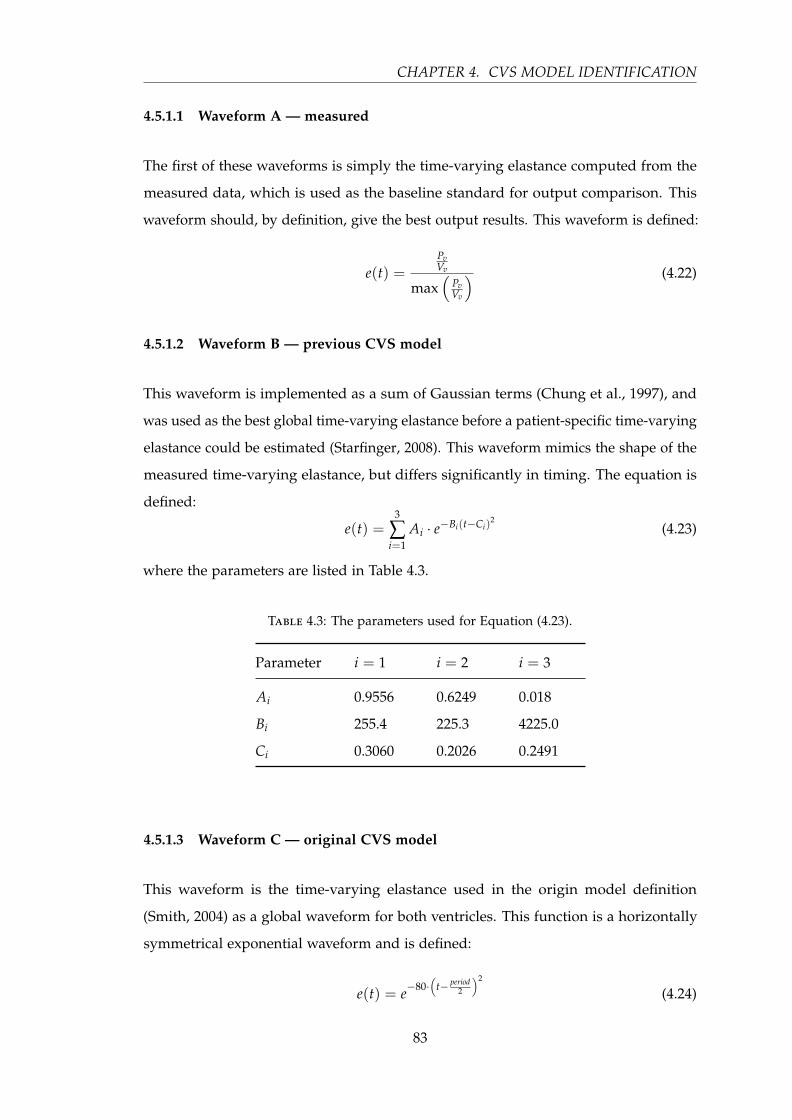
CHAPTER 4. CVS MODEL IDENTIFICATION
4.5.1.1 Waveform A — measured
The first of these waveforms is simply the time-varying elastance computed from the
measured data, which is used as the baseline standard for output comparison. This
waveform should, by definition, give the best output results. This waveform is defined:
e(t) =PvVv
max(
PvVv
) (4.22)
4.5.1.2 Waveform B — previous CVS model
This waveform is implemented as a sum of Gaussian terms (Chung et al., 1997), and
was used as the best global time-varying elastance before a patient-specific time-varying
elastance could be estimated (Starfinger, 2008). This waveform mimics the shape of the
measured time-varying elastance, but differs significantly in timing. The equation is
defined:
e(t) =3
∑i=1
Ai · e−Bi(t−Ci)2
(4.23)
where the parameters are listed in Table 4.3.
Table 4.3: The parameters used for Equation (4.23).
Parameter i = 1 i = 2 i = 3
Ai 0.9556 0.6249 0.018
Bi 255.4 225.3 4225.0
Ci 0.3060 0.2026 0.2491
4.5.1.3 Waveform C — original CVS model
This waveform is the time-varying elastance used in the origin model definition
(Smith, 2004) as a global waveform for both ventricles. This function is a horizontally
symmetrical exponential waveform and is defined:
e(t) = e−80·(
t− period2
)2
(4.24)
83

4.5. TIME-VARYING ELASTANCE (TVE)
4.5.1.4 Waveform D — universal
When the time-varying elastance was initially conceived, it was thought that every
time-varying elastance had the same normalised shape (Suga et al., 1973). This shape,
as published by Suga et al. (1973), is waveform D.
4.5.1.5 Waveform E — square
This waveform is included, not as a realistic time-varying elastance, but as a test of
the limitations of the model to extreme time-varying elastance slopes. This waveform
is implemented by rounding the measured time-varying elastance to 1 or 0, and
smoothing the corners to avoid discontinuities.
4.5.1.6 Waveform F — linear piecewise
This waveform is a simple linear piecewise representation of the time-varying elastance
mimicking the basic shape. The waveform was lightly smoothed to avoid discontinuities
at the corners.
4.5.2 Model responses to different TVE waveforms
To see the sensitivity of the model to the time-varying elastance, three outputs of
the model are shown, the left ventricle pressure, Plv, the aortic pressure, Pao and the
pulmonary vein pressure, Ppu.
Figure 4.7 shows the left ventricle pressure for each of the time-varying elastances
in Figure 4.6. It is clear from the aortic pressure of the model that the time-varying
elastance plays a significant role in many aspects of the aortic pressure waveform,
including the shape, height and timing. It should be noted, that no other time-
varying elastance comes close to matching the output from the measured time-varying
elastance of waveform A. The universal time-varying elastance (Suga et al., 1973)
significantly underestimates the peak pressure of the left ventricle, where the square
wave significantly overestimates it. The key difference here is the slope of the rising
84
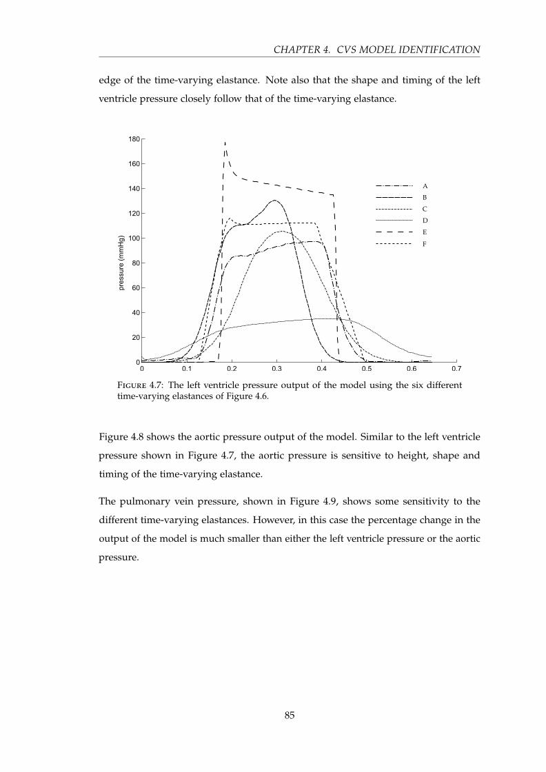
CHAPTER 4. CVS MODEL IDENTIFICATION
edge of the time-varying elastance. Note also that the shape and timing of the left
ventricle pressure closely follow that of the time-varying elastance.
Figure 4.7: The left ventricle pressure output of the model using the six differenttime-varying elastances of Figure 4.6.
Figure 4.8 shows the aortic pressure output of the model. Similar to the left ventricle
pressure shown in Figure 4.7, the aortic pressure is sensitive to height, shape and
timing of the time-varying elastance.
The pulmonary vein pressure, shown in Figure 4.9, shows some sensitivity to the
different time-varying elastances. However, in this case the percentage change in the
output of the model is much smaller than either the left ventricle pressure or the aortic
pressure.
85
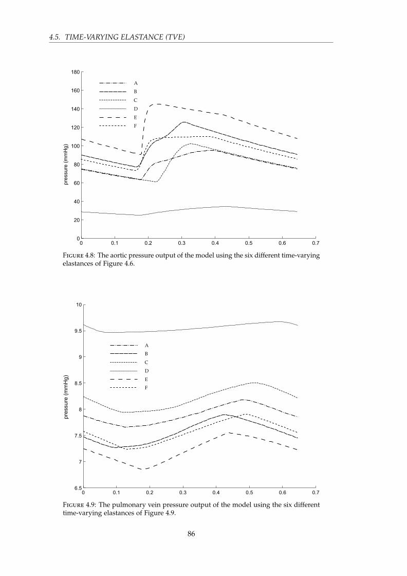
4.5. TIME-VARYING ELASTANCE (TVE)
Figure 4.8: The aortic pressure output of the model using the six different time-varyingelastances of Figure 4.6.
Figure 4.9: The pulmonary vein pressure output of the model using the six differenttime-varying elastances of Figure 4.9.
86

CHAPTER 4. CVS MODEL IDENTIFICATION
4.6 Discussion
4.6.1 Parameter identification limitations
A significant limitation on the identification algorithm outlined in this chapter is its
reliance on the pulmonary artery pressure, Ppa which, when measured, is usually done
with a pulmonary artery catheter (PAC). The use of a PAC is not as common as formerly
(Johnston et al., 2008; Wiener and Welch, 2007), perhaps due to the questionable or
negative effects its use has had on mortality rates (Binanay et al., 2005; Shah et al.,
2005). However, it is most likely that the value of the PAC has more to do with the
interpretation of the resulting waveforms than the presence of the catheter itself (Shah
et al., 2005). Any catheterisation comes with added risk. However, the additional risks
of a PAC are regarded as small (Berenholtz et al., 2004; Johnston et al., 2008; Mermel,
1991; Ramritu et al., 2008; Safdar et al., 2002; Weil, 1998). Therefore, with the correct
understanding of the data acquired from a PAC, the clinical advantages can be realised.
There are many features of the pulmonary artery pressure waveform that can be of
clinical use if extracted correctly from the waveform. These metrics include, ventricular
contractility, preload, vascular stiffness and resistance. Therefore there is a strong case
for the use of a PAC when combined with modelling techniques such as those outlined
by the model presented here.
It should also be noted that the identification method could be reformulated to use
measurements from echocardiography to eliminate the use of a PAC. However, this
approach would significantly reduce the frequency of identification and thus the use
of the model, and increase the financial cost. Specifically, echocardiography is not
real-time and involves significant clinical effort.
One more limitation of the identification algorithm is the assumption that Vd,lvf =
Vd,rvf = 0. In most cases the true values would be non-zero, but are currently unrealistic
to measure or identify. The result of this assumption is a slightly different definition of
the ventricular contractility from the accepted gold standard (Suga et al., 1973; Sagawa
et al., 1977). Thus, the absolute values of Ees,lvf and Ees,rvf as identified by the model
will not match this gold standard. However, due to the lumped parameter nature of
the model, and given that physiological values of the dead space volume stay relatively
constant, the identified trends in the contractility will track those of the originally
87

4.7. SUMMARY
defined gold standard contractility. Hence, the original assumption does not impact on
the clinical use.
4.6.2 Sensitivity to the time-varying elastance
It has been shown that the correct time-varying elastance waveform is of critical
importance to the simulation of the model in Figures 4.7–4.9, and thus also, the
identification, as both rely heavily on model simulation involving the time-varying
elastance. Even though it is not realistic to fully quantify the exact sensitivity of the
model to the time-varying elastance, or attempt to state, in any meaningful way, the
interaction between the model outputs and the time-varying elastance, the simulations
with different time-varying elastance in Figures 4.7–4.9 give clear visual illustrations of
the sensitivity.
Ultimately, the best result for the model and its identification would be to measure the
patient-specific time-varying elastance. Currently, this measurement is not achievable
in a clinical setting due to the invasiveness of the procedures required. However, a
patient-specific estimation of the time-varying elastance is possible and is presented
and discussed in Chapters 6 and 7, as a main outcome of this thesis.
4.7 Summary
This chapter has presented an algorithm for identifying the parameters of the six-
chamber model described in Chapter 3. The method uses only measurements that
are commonly available in an ICU setting, and provides a robust way to obtain a
model that accurately mimics the major haemodynamics of a patient. It has also been
demonstrated that an accurate time-varying elastance is required for the simulation of
the model and thus, in addition, its identification.
88

Chapter 5
Time-Varying Elastance
This chapter outlines the development of the time-varying elastance concept, from its
initial conception to its current usage and implications. Three major aspects of the
time-varying elastance model are discussed, namely the index of contractility, the total
mechanical energy of the contracting ventricles, and its usage in lumped parameter
models of the cardiovascular system.
5.1 Introduction
The time-varying elastance concept is an elegant and simple approach to representing
the contraction of the myocardium. The time-varying elastance model is a high level
approach to mathematically represent the dynamics of a ventricle. As such, it does
not directly account for the mechanics of contraction. However, it has had much
success in several areas (Cooper, 1990; Suga, 1990b), including the derivation of the
total mechanical energy of the heart, which to some is a surprising result that seems to
go deeper into the mechanics of the ventricle than the conceptual model would allow
(Cooper, 1990).
Certain aspects of time-varying elastance concept have had much debate in the literature.
These include the linearity and load-independence of the end-systole pressure-volume
relationship (Burkhoff et al., 1987; Kass et al., 1989; Baan and Velde, 1988; Burkhoff et al.,
1993; Oommen et al., 2003; Mirsky et al., 1987; Su and Crozatier, 1989; Velde et al., 1991;
Noda et al., 1993; Kameyama et al., 1998; Lee et al., 1998), along with the universality of
89

5.2. HISTORIC CONTEXT
the height and time-to-end-systole normalised time-varying elastance waveform (Jegger
et al., 2007; Palmer et al., 2004; Kjorstad et al., 2002). Much of this debate focuses on what
is within physiological range, and what can be deemed an appropriate approximation
for the context of the model under question. What appears to be generally accepted is
the success of the conceptual model both in providing information regarding ventricular
energetics and as an input to larger lumped parameter models of the cardiovascular
system. As such, the model has taken a firm hold in the physiological understanding
of the cardiovascular system.
5.2 Historic context
Metabolic cost of contraction has been studied for many years, with initial studies in the
mid 19th century linking chemical change and heat production to muscle contraction
(Helmholtz, 1845, 1848). This understanding was further formalised, and a relation was
recognised between tension generation and oxygen consumption (Evans and Matsuoka,
1915; Rohde, 1912), with developed tension shown to be a major determinant of left
ventricular oxygen consumption (McDonald et al., 1966; Neely et al., 1967; Rodbard
et al., 1964; Sarnoff et al., 1958; Weber and Janicki, 1977). The understanding that the
metabolic cost of the cardiac contraction can be described in terms of oxygen consump-
tion (Challoner, 1968) was a major step forward in the understanding of the energetic
cost of contraction. From this background, Sonnenblick (1962) established a widely
used index of contractility, Vmax, representing the maximum unloaded shortening
velocity of the myocardium (Karliner et al., 1971).
A parallel movement to conceptualise the energetics of the heart focused on the fluid
dynamic aspects of cardiac function. This line of study was pioneered by the German
physiologist Otto Frank who characterised ventricular contraction in a pressure-volume
diagram (Frank, 1899; Sagawa et al., 1990). The British physiologist Ernest Starling,
extended the work done by Frank on frog hearts, to canine preparations, and developed
a relationship between cardiac output and filling pressure, known as Starling’s law of
the heart (Starling, 1918). Sarnoff and Berglund (1954) later modified Starling’s curve
to develop a ventricular function curve (Sarnoff and Berglund, 1954) which, together,
were used to visualise inotropism and contractility changes.
90
CHAPTER 5. TIME-VARYING ELASTANCE
Discontented with Sonnenblick’s concept of a contractility index, Vmax, Suga et al. (1973),
established the long standing (and still current) index of contractility based on a model
of the elastance of the ventricular muscle, namely, Emax (Suga et al., 1973). Suga and
Sagawa (1974) then followed with a wealth of publications embedding Emax in clinical
usage, and formalising the time-varying elastance model of cardiac dynamics (Warner,
1959; Suga and Sagawa, 1974). Further works linked the fluid dynamic concept of the
pressure-volume construction to the metabolic cost represented by oxygen consumption
(Suga, 1969b, 1970).
5.3 Maximal elastance, time-varying elastance and the
pressure-volume diagram
The time-varying elastance model is a broad concept that has been used in many
ways. The most prominent include the index of contractility, Emax, the measure of total
mechanical energy as the area inside the pressure-volume diagram, and as part of
lumped parameter cardiovascular models. The first of these, Emax – the line connecting
the points of end-systole on the pressure-volume diagram – was suggested to be essen-
tially linear and proportional to contractility (Suga, 1970, 1969a,b, 1971a,b). Suga and
Sagawa (1972) concluded that the left ventricle performance could be characterised by
a time-varying elastance, E(t) (Suga and Sagawa, 1972), and showed that when nor-
malised to height and time-to-end-systole, the time-varying elastance was independent
of loading conditions (Suga et al., 1973; Suga and Sagawa, 1974). These key findings
have stayed central to the understanding of cardiac energetics both in cardiovascular
research and clinical practice (Hall and Guyton, 2011; Westerhof et al., 2010; Burkhoff,
2009; Campbell et al., 2008).
5.3.1 Maximal elastance, Emax
The concept of using Emax as a measure of contractility came from empirical studies
done by Suga et al. in the late 1960s and early 1970s. These studies showed a remarkably
linear relationship between end-systolic pressure and volume, with the slope being
insensitive to loading conditions and type of contraction, as well as being sensitive to
91

5.3. MAXIMAL ELASTANCE, TIME-VARYING ELASTANCE AND THEPRESSURE-VOLUME DIAGRAM
the contractile state (Suga et al., 1973; Suga and Sagawa, 1974). Figure 5.1 illustrates
the general concept of Emax and how it changes with a change in the contractile state.
Figure 5.1: Left ventricular pressure-volume loops of a denervated heart, adaptedfrom (Suga et al., 1973). The arterial pressure was fixed at three different levels, foreach of a control state and an enhanced contractile state.
Despite the controversy about the load-independence and linearity of Emax (Burkhoff
et al., 1987; Kass et al., 1989; Baan and Velde, 1988; Burkhoff et al., 1993; Oommen et al.,
2003; Mirsky et al., 1987; Su and Crozatier, 1989; Velde et al., 1991; Noda et al., 1993;
Kameyama et al., 1998; Lee et al., 1998), it is generally acknowledged to be basically
linear and load-independent within the physiological range (Kind et al., 2009; Noda
et al., 1993; Brinke et al., 2010). This acceptance is evidenced by its extensive use, which,
in most cases, depends on its linearity and load-independence. Although it has gained
widespread acceptance as being a good measure of contractility (Sagawa, 1981; Kass,
1992; Takaoka et al., 1993; Senzaki et al., 1996; Shishido et al., 2000), Emax has had
limited uptake in clinical environments due to the relative difficulty of measuring it in
a clinical setting (Shishido et al., 2000; Brinke et al., 2010).
92

CHAPTER 5. TIME-VARYING ELASTANCE
The most common and reliable way to measure Emax is by recording multiple cardiac
pressure-volume loops over a range of volumes, usually through reducing preload via
an inferior vena cava occlusion (Kass, 1992). Although feasible, this method is invasive
and therefore inappropriate for patients with advanced heart failure. Many attempts
have been made to estimate Emax, and, in so doing, give more accessibility to the index
in a clinical setting. The majority of attempts have focused on reducing the need for
the vena cava occlusion manoeuvre, by requiring only a single PV loop (Klotz et al.,
2006; Takeuchi et al., 1991; Senzaki et al., 1996; Shih et al., 1997; Shishido et al., 2000;
Kjorstad et al., 2002).
Emax fits into a bigger modelling picture as the maximum elastance of the time-varying
elastance concept. However, Emax as a measure of contractility, can be derived, as
originally, from the end-systolic pressure-volume relationship. Emax is the most sought-
after metric from the time-varying elastance concept, due to its clinical significance.
Thus, it is used extensively in animal research and increasingly as a clinical tool to
gauge cardiac pump function (Westerhof et al., 2010).
Another extension of the Emax concept is the value of the dead space volume Vd (Suga
et al., 1973), which is the volume intercept of ESPVR. It is generally assumed that
ESPVR is linear, and thus Vd is found as an extrapolation of ESPVR. However, ESPVR
is non-linear (Claessens et al., 2006), and the non-linearity depends on the contractility
(Sato et al., 1998). Therefore, for higher contractilities, Vd will be underestimated, often
significantly (Westerhof et al., 2010) using a linear assumption. For this reason, an
accurate Vd can be very hard to obtain in a clinical setting, not to mention the invasive
nature of the required measurements.
5.3.2 Time-varying elastance (TVE)
Although the use of compliance, or its inverse, elastance, was not new (Warner, 1959),
Suga et al. (1973) formalised the concept of a time-varying elastance to characterise
the fluid dynamics of the left ventricle. This resulted from the observation that the
relationship between pressure and volume in the left ventricle could be accurately
approximated by (Suga et al., 1973):
P(t) = E(t) · (V(t)−Vd) (5.1)
93

5.3. MAXIMAL ELASTANCE, TIME-VARYING ELASTANCE AND THEPRESSURE-VOLUME DIAGRAM
where P(t) is the instantaneous intraventricular pressure, E(t) is the time-varying slope
coefficient of the regression line of pressure and volume, V(t) is the instantaneous
intraventricular volume, and Vd is the volume at zero pressure (dead space volume),
defined, at the time, as the fixed correction volume.
From this observation the pressure-volume regression line E(t) can be constructed in
its own right, and given the name time-varying elastance. The dead space volume was
assumed constant, although in reality its value decreases with time in the early phase of
systole (Sagawa, 1978), remaining virtually constant from around 80 ms onwards. Thus,
the value of Vd was typically taken as constant with the end-systolic value (Sagawa,
1978).
Figure 5.2 shows a pressure-volume diagram with isochrone regression lines at specific
points all connected to the dead space volume, Vd, with these time points also shown
on the time-varying elastance curve. The slopes of these lines, when continuously
connected around the entire PV loop, construct E(t).
Figure 5.2: Isochrone regression lines at times, t0, t1, t2 and t4, all connected to thedead space volume, Vd (left), and the equivalent time points on the time-varyingelastance curve (right).
The curve E(t) that Suga et al. (1973) produced, was a by-product of the goal to
conceptualise and visualise the contractility and energetics of the heart. The concept of
Emax, which was developed first, was extended to cover the entire systolic phase, and,
eventually the entire cardiac cycle, even though the authors noted that the equation
for E(t) – Equation (5.1) rearranged for E(t) – was not valid for diastole (Sagawa,
1978). Therefore, Emax and the total mechanical energy concept of pressure-volume area
(PVA) were the main focus of most of their research (Suga, 1990b). The concept of the
94

CHAPTER 5. TIME-VARYING ELASTANCE
time-varying elastance was thus left as a foundation for properties such as Emax and
PVA. As a result the intrinsic properties of the time-varying elastance, as a waveform,
for diagnostic and clinical potential were largely neglected.
Comparison of time and value normalised E(t) curves, En(tn), obtained under different
contractile conditions, showed similar shapes. This result led Suga et al. (1973) to the
conclusion that Emax, the maximum value of E(t), and Tmax, the time to Emax, could
be considered the characteristic parameters of the instantaneous pressure-volume
ratio curve (Suga et al., 1973). In other words, the time-varying elastance was largely
independent of loading conditions and mode of contraction, at least during systole.
The model represented by Equation (5.1) is a one-element time-varying elastance model,
equivalent to a circuit consisting of a single variable capacitor connected to a load, as
shown in Figure 5.3. Other models exist, such as a two- and three-element model, that
attempt to account for additional pressure loss and a constant portion of elastance
(Zhong et al., 2005). However, the two- and three-element models have not received as
much attention in the literature, likely due to added complexity and limited quality
data to justify them.
Figure 5.3: A one (left) and three (right) element time-varying elastance model. Theload, when applied to the cardiovascular context, is the arterial load.
Since the initial conception of the one element model, there have been many attempts
to improve the model, primarily in recognition that the left ventricular pressure is
dependant on flow and thus the loading conditions (Hunter et al., 1979, 1983; Shroff
et al., 1985; Templeton et al., 1972; Vaartjes and Boom, 1987). This issue is especially
valid during ejection and relaxation (Campbell et al., 2008). In fact, the first such
95

5.3. MAXIMAL ELASTANCE, TIME-VARYING ELASTANCE AND THEPRESSURE-VOLUME DIAGRAM
model improvement came from the original authors (Suga et al., 1980), extending the
one-element model to a three-element model shown in Figure 5.3.
Shroff et al. (1983) developed a more involved model, containing elastance, resistance
and inductance, all three of which depend on time, pressure, volume, flow and
flow acceleration (Shroff et al., 1983). Inertia was found to be negligible, while the
resistance helped adjust for the known pressure errors in the previous one-element
model (Suga et al., 1980). Viscous and passive elastic elements have also been added to
the original time-varying elastance concept (Hunter et al., 1983). Wijkstra and Boom
(1991) revamped the three element model (Suga et al., 1980), with a similar motivation
leading to the introduction of flow dependence into the model (Wijkstra and Boom,
1991). Finally, the addition of a second, stiffer series elastance was shown to better
predict lag in the ventricle pressure drop after a stepwise increase in ejection flow
(Covell et al., 1975; Schiereck and Boom, 1978; Templeton et al., 1972; Vaartjes and
Boom, 1987; Yasumura et al., 1989b).
Models are still being developed with similar attention to flow and load dependence.
Zhong et al. (2005) uses a passive and active elastance model (Zhong et al., 2005) to
account for a filling resistance, while Kind et al. (2009) showed a load-dependence
on the time course of contraction and cardiac timing (Kind et al., 2009). This load
dependence was based on observations in rats (Lee et al., 1998), mice (Claessens et al.,
2006), and dogs (Burkhoff et al., 1987; Kass et al., 1989; Velde et al., 1991) that isochrones
and the ESPVR are generally non-linear and that their non-linearity depends on the
contractile state of the heart (Sato et al., 1998). The solution that Kind et al. (2009)
developed involved a time-normalisation of the four cardiac phases and the use of
isophase lines instead of the isochrones that are generally used (Kind et al., 2009).
Hence, significant advances in models and understanding have been made from the
original load independent models and assumptions.
Along with the assumption of load-independence, many studies have shown that
En(tn) has a similar shape irrespective of loading, disease state and species, leading
to the conclusion of a universal time-varying elastance shape (Suga et al., 1973; Sen-
zaki et al., 1996; Georgakopoulos et al., 1998). Senzaki et al. (1996) showed that the
normalised time-varying elastance was independent of different cardiac pathologies,
contractility, preload and afterload (Senzaki et al., 1996), and the same group followed
96

CHAPTER 5. TIME-VARYING ELASTANCE
with results showing the shape of the normalised time-varying elastance was identical
in different animal species (Georgakopoulos et al., 1998). From these results Senzaki
et al. (1996) assumed the universality of the time-varying elastance, and proposed a
method to estimate the time-varying elastance from a single pressure-volume loop
which had important clinical implications (Senzaki et al., 1996). Several other groups
have attempted similar things (Hayashi et al., 2000; Lee et al., 2002; McKay et al., 1986).
However, there is no consensus in the literature that in fact the normalised time-varying
elastance is universal (Jegger et al., 2007). En(tn) has been found to be inaccurate or
not applicable to the single-beat methodology (Kjorstad et al., 2002), and in fact, the
results of Senzaki et al. (1996) are not all that compelling to support the assumption of
a universal time-varying elastance (Jegger et al., 2007; Senzaki et al., 1996).
The overall simplified model of the time-varying elastance as first proposed (Suga et al.,
1973), and most widely used today, has its limitations in the curve-linearity of ESPVR,
afterload dependence of E(t) and the variability of the dead space volume Vd (Little
and Freeman, 1987; Sato et al., 1998; Shishido et al., 2000). However, it has been widely
used to great success, especially as the input to lumped parameter models. These
models range in their intended purpose, from specific to quite general, and vary in the
amount of the circulation they attempt to simulate. Single chamber models exist for
the left ventricle, which use the time-varying elastance concept as an input (Avanzolini
et al., 1985), along with full-system models intended to study the ventricles and their
interaction (Santamore and Burkhoff, 1991; Amoore et al., 1992). More generalised
full-system models based on the underlying time-varying elastance concept range from
a minimalistic approach (Starfinger et al., 2007; Burkhoff and Tyberg, 1993; Olansen
et al., 2000) to the very complex (Liang and Liu, 2005; Sun et al., 1997; Kappel et al.,
2007).
The range of model size and complexity that utilises the concept of the time-varying
elastance gives credibility to the use of such an assumption, as well as the reliability
and physiological relevance of the model, despite the concern by some researchers that
time-varying elastance is purely a phenomenological assertion (Loiselle et al., 2008;
Cooper, 1990; Landesberg et al., 1993; Claessens et al., 2006; Campbell et al., 2008).
97

5.3. MAXIMAL ELASTANCE, TIME-VARYING ELASTANCE AND THEPRESSURE-VOLUME DIAGRAM
5.3.3 Pressure-volume area
Following on from the work to understand Emax and E(t), Suga (1979b) theorised
that the total mechanical energy of a contraction could be deduced from the E(t)
model (Suga, 1979b). This idea comes from the physics of the time-varying elastance
model relating to mechanical energy, and is validated by correlations with oxygen
consumption. Given that the heart relies almost exclusively on oxidative metabolism for
energy generation, this approach thus assumes that the rate of oxygen consumption can
provide an adequate measure of the total energy utilization (Suga, 1979b; Braunwald,
1976). This conceptual framework not only validates the total mechanical energy
derivation, but gives more weight to the physiological significance of the time-varying
model itself.
The pressure-volume diagram and time-varying elastance are linked concepts, although
they can be used independently. The PV diagram is a trace of the time-varying elastance
on a different set of coordinates, namely pressure and volume. Although the correlation
for oxygen consumption and mechanical work comes from the PV diagram, it is the
underlying model of mechanical elasticity, the time-varying elastance model, that
allows an analytical formulation of mechanical energy giving physiological backing to
the correlation (Suga, 1979b).
For an ideal elastic material, the potential energy at a stretch length xs, can be calculated:
PE =∫ xs
0f (x)dx (5.2)
where f (x) is a length-dependant force function (Suga, 1979b). For a linear material,
this equation becomes PE = 12 · kx2 where k is the slope of the linear force-length
relation. For any function f , the potential energy is the area under f .
The time-varying elastance concept is that of a special elastic material, whose spring
constant changes with time, although at any one instant its force-length relation is still
linear. A major difference between this approach, and a normal elastic material, is
that potential energy can be generated without any additional stretch by increasing
the stiffness of the material. In both cases, the potential energy at any instant in time
is independent of the stretch history. This approach thus implies that the potential
energy remaining in the ventricle at the end of systole is the area of the triangle below
98

CHAPTER 5. TIME-VARYING ELASTANCE
the ESPVR line, between the volume axis and the point of end-systole, as shown in
Figure 5.4.
Figure 5.4: The total mechanical energy for a contracting ventricle as represented bythe sum of the work done by the ventricle (light grey area) and the potential energyremaining in the muscle at the end of systole (dark grey area).
The second part of the energetic analysis of the ventricle contraction is the actual work
done during contraction. In a similar fashion to the potential energy, the work done is
the integral of the line traced during systole on the PV diagram, shown in Figure 5.4.
Therefore, the total energy required for a contraction equates to the work done during
the contraction, plus the potential energy remaining in the material at the end of systole.
Note that the area, or energy, under the end-diastolic pressure-volume curve is left out
of this mechanical energy formulation, as this energy does not appear to be actively
supplied (Monroe and French, 1960; Suga, 1979b).
It is this formulation of total mechanical energy (work done plus potential energy)
that correlated linearly with oxygen consumption under various preload and afterload
conditions (Suga, 1990b; Loiselle et al., 2008), validating it as a useful metric of cardiac
energetics (Suga, 1990b, 1979b). A further implication of this energetic concept and
99
5.4. DISCUSSION
formulation is that it allows the myocardial contractile efficiency to be determined
directly (Suga et al., 1986, 1984).
The pressure-volume-area approach to mechanical cardiac performance has some major
advantages over methods that use contractile parameters, such as force and shortening
velocity (Kass and Maughan, 1988; Katz, 1988). However, two short-comings of the
PVA approach as compared to load and heat have been outlined (Suga, 1990b). First,
the fraction of myocardial oxygen consumption cannot generally be isolated from that
of contractile events (Suga et al., 1983; Yasumura et al., 1989a). Second, the fractions
for initial heat cannot be separated from that of recovery heat (Gibbs and Chapman,
1985; Suga et al., 1986). Despite these minor drawbacks, this approach has had much
attention in both literature and physiological textbooks.
5.4 Discussion
The concept of the time-varying elastance is well established and successful in animal
research, but has made only minor advances into the clinical environment, beyond that
of a purely academic understanding of the heart. The concept of maximal elastance
is firmly grounded as the gold standard for measurement of ventricular contractility
despite the clinical difficulties of measuring it. To this end, many researchers, with
varying degrees of success, have tried to find less invasive means to obtain a measure
of Emax (Senzaki et al., 1996; Guarini et al., 1998; Swamy et al., 2009; Shishido et al.,
2000; Brinke et al., 2010).
Although much is understood about the time-varying elastance concept, there are two
areas which remain controversial. These are the load-independence, and universality
of the time-varying elastance shape. The initial concept (Suga et al., 1973) suggested
this load-independence and universality, and it seems to have moved from a general
rule to a physiological law, despite the range of publications suggesting otherwise.
Perhaps this is because of the success of the contractile index that partially relies on
such a load-independence. However, this index of contractility is only one aspect of
the overall time-varying elastance concept. It should be clear that at a fundamental
level, the time-varying elastance is dependent on loading conditions, simply by the
number of attempts to improve the one-element model by including load dependent
100

CHAPTER 5. TIME-VARYING ELASTANCE
variables such as flow (Hunter et al., 1979, 1983; Shroff et al., 1985; Templeton et al.,
1972; Vaartjes and Boom, 1987). There is also no underlying necessity for the model to
be load-independent, rather this property was inferred from empirical measurements,
not from the conception of the model or the underlying physiology (Suga et al., 1973).
In fact, to some, the model deviates from physiology far enough for it to be considered
surprising that the time-varying elastance concept is as successful as it has been in
describing the state of the ventricles (Cooper, 1990).
The universality of the normalised time-varying elastance has seen less attention and
controversy in the literature, perhaps because this assumption is required by fewer
models and clinical implications and thus has been less important. However, this is
a growing area, with estimations of the Emax relying on the universality of the time-
varying elastance, as well as other estimations relying on the opposite assumption, see
Chapter 8.
Lumped parameter models of the cardiovascular system have long relied on the time-
varying elastance of the ventricles as an input function. As such, the time-varying
elastance becomes a driver for the model, and is thus usually validated based on the
success of the overall cardiovascular model, rather than of the physiological meaning
and accuracy of the time-varying elastance itself. In fact, most of the attempts to
estimate and model the time-varying elastance are based on this indirect form of
validation (Senzaki et al., 1996; Guarini et al., 1998; Swamy et al., 2009; Shishido et al.,
2000; Brinke et al., 2010). There is nothing wrong with using an indirect form of
validation, provided the context stays within the bounds of the validation. However,
due to the physiological nature of the time-varying elastance model, its success in
describing the contractile state, and the total mechanical energy of the heart, it would be
reasonable to expect that an estimation of the time-varying elastance could be validated
on its own merits (Stevenson et al., 2012b).
5.5 Summary
This chapter has presented the evolution of the time-varying elastance concept, and
implications arising from aspects of the model such as the contractile index, Emax, and
the total mechanical energy of the heart. The overall model has remained a central part
101

5.5. SUMMARY
of the understanding of the cardiovascular system in research, textbooks and clinical
application, although direct clinical application has yet to see major advances due to
the invasiveness of the procedures required to obtain measurements of the waveforms.
There is also controversy in the literature on specific assumptions that can be made
surrounding the time-varying elastance concept, specifically the load-independence
and universality of the time and value normalised shape of the waveform. Despite this
controversy, the overall concept is well accepted in many areas, most notably as an
index of contractility and as an input to lumped parameter models of the cardiovascular
system.
102

Chapter 6
Processing the aortic and pulmonary
artery pressure waveforms
This chapter presents the first half of the process of estimating the ventricular time-
varying elastance. Specifically, the processing of the aortic and pulmonary artery
pressure waveforms to extract the required data. Specific points on these two waveforms
are required by the algorithms developed in Chapter 7 to estimate the time-varying
elastance. To estimate the time-varying elastance algorithmically at the bedside, the
required points on the pressure waveforms must be able to be automatically extracted
in a reliable and accurate way.
6.1 Introduction
There is much data available in an ICU setting. However, much of that data is effectively
lost due to it being hidden deep in the waveforms displayed to the clinician. To extract
that information, complex models are needed to process the waveforms and give
clinical and physiological meaning to the numerical data. This approach creates a
physiological picture from complex dynamics embedded in the waveform, acting to
clarify the data presented into a clinical context.
There are also waveforms that cannot be measured in an ICU setting, such as the time-
varying elastance, due to the invasive nature of the required procedure. In the literature
to date, this particular waveform has not had much attention in a clinical context, as it
103

6.2. METHODS
is not considered practical to measure in humans. However, the time-varying elastance
has much to offer the clinician in the way of diagnostic potential, as the measurement is
so closely linked to the energetics of the heart, and thus the state of the heart’s function.
The only way to access the information content of the time-varying elastance is to
estimate this waveform from other data and waveforms that are practical to measure.
A second motivation to obtain the time-varying elastance waveform is to provide a
required input for the cardiovascular system model, discussed in Chapter 3. This input
provides the driving force behind the model, and is often referred to as the driver
function. Previously, a global approximation has been used as the input, which, by
nature, does not take into account any patient-specific deviation from this less-than-
ideal approximation. As was shown in Chapter 4, the time-varying elastance has
significant influence on the model outputs. A patient’s specific function would thus
offer significant clinical potential beyond its direct value.
The general approach to approximate the time-varying elastance can be divided into
two halves. First, specific points need to be extracted from the pressure waveforms.
Second, using predetermined correlations, these points are correlated to specific points
on the time-varying elastance waveform. From these general correlations a curve can be
drawn forming the final approximated waveform. The measured pressure waveforms
of the aortic and pulmonary artery pressures can be noisy and/or biased in such a way
as to make extracting the required points non trivial. Hence, initial signal processing is
required, which is the focus of this chapter.
6.2 Methods
A high-level view of this approach is presented in Figure 6.1, which shows the formation
and use of the correlations to generate estimated time-varying elastance waveforms.
This chapter is focused on the left half of Figure 6.1, that of extracting data from the
pressure waveforms for later use.
The overall method described here, and in Chapter 7, is shown in Figure 6.2. However,
this approach is useful if and only if it is possible to automate the detection of the
required points, defined in Equation (6.1), on the aortic pressure, Pao, and pulmonary
artery pressure, Ppa, waveforms, which are shown in Figures 6.3 and 6.4.
104

CHAPTER 6. PROCESSING THE AORTIC AND PULMONARY ARTERY PRESSUREWAVEFORMS
Figure 6.1: The figure shows a conceptualised overview of the process described inthis chapter and Chapter 7, and further implications. From the many measured leftventricular time-varying elastance waveforms, elv(t), along with many aortic pressurewaveforms, Pao, correlations are derived — the information flow is shown through thelarge grey arrow. Once these correlations are known, they can be used along with theaortic pressure waveform (from a specific patient), to arrive at an estimation of theirtime-varying elastance waveform. The equivalent for the right side is also shown.
Figure 6.2: To illustrate what can be done with the identified points on the aorticpressure, an example of the formation of the estimated time-varying elastance elastanceis shown here, while the terms are defined in Equation (6.1).
105
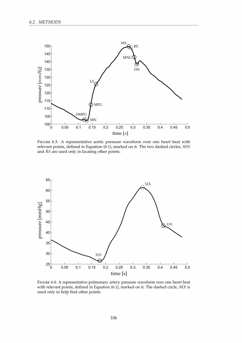
6.2. METHODS
Figure 6.3: A representative aortic pressure waveform over one heart beat withrelevant points, defined in Equation (6.1), marked on it. The two dashed circles, MNand RS are used only in locating other points.
Figure 6.4: A representative pulmonary artery pressure waveform over one heart beatwith relevant points, defined in Equation (6.1), marked on it. The dashed circle, MX isused only to help find other points.
106

CHAPTER 6. PROCESSING THE AORTIC AND PULMONARY ARTERY PRESSUREWAVEFORMS
To begin, a naming convention is defined:
e(t) ≡ ventricular time varying elastance
Pao ≡ aortic pressure
Ppa ≡ pulmonary artery pressure
DMPG ≡ driver maximum positive gradient
MN ≡ minimum point
MPG ≡ maximum positive gradient
LS ≡ left shoulder
MX ≡ maximum
RS ≡ right shoulder
MNG ≡ maximum negative gradient
DN ≡ dicrotic notch
(6.1)
6.3 Shear Transform
A shear transform is defined to aid feature extraction from the measured Pao and Ppa
waveforms. This transform is defined:
S ≡ (t, X(t))→ (t, φshear(X(t))) (6.2)
where:
φshear (X(t)) = X(t) + mt + c, t0 < t < tend (6.3)
X(t) ≡ discrete, time valued data (6.4)
and the parameters t0 and tend are set depending on the region or period of interest.
The parameters m and c are chosen such that:
φshear(X(t0)) = X(t0) = φshear(X(tend)) (6.5)
107
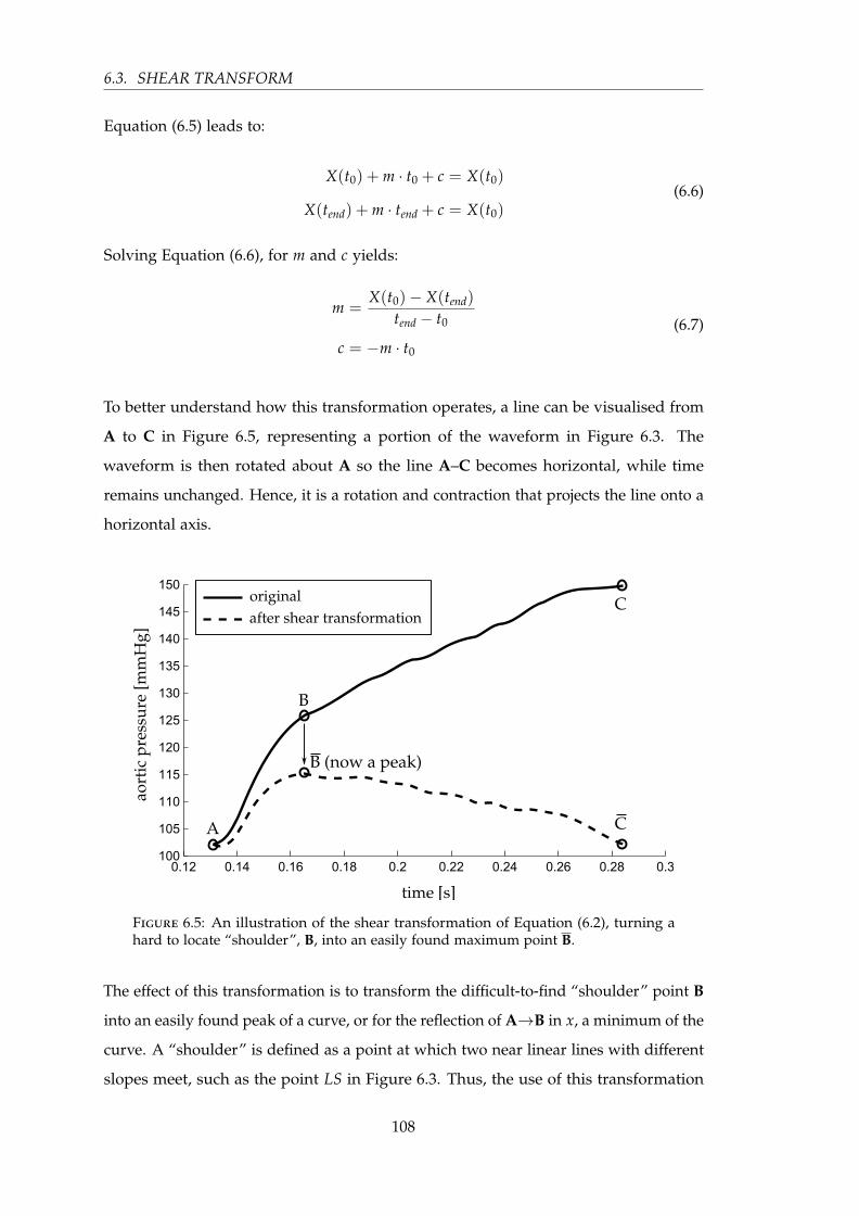
6.3. SHEAR TRANSFORM
Equation (6.5) leads to:
X(t0) + m · t0 + c = X(t0)
X(tend) + m · tend + c = X(t0)(6.6)
Solving Equation (6.6), for m and c yields:
m =X(t0)− X(tend)
tend − t0
c = −m · t0
(6.7)
To better understand how this transformation operates, a line can be visualised from
A to C in Figure 6.5, representing a portion of the waveform in Figure 6.3. The
waveform is then rotated about A so the line A–C becomes horizontal, while time
remains unchanged. Hence, it is a rotation and contraction that projects the line onto a
horizontal axis.
Figure 6.5: An illustration of the shear transformation of Equation (6.2), turning ahard to locate “shoulder”, B, into an easily found maximum point B.
The effect of this transformation is to transform the difficult-to-find “shoulder” point B
into an easily found peak of a curve, or for the reflection of A→B in x, a minimum of the
curve. A “shoulder” is defined as a point at which two near linear lines with different
slopes meet, such as the point LS in Figure 6.3. Thus, the use of this transformation
108
CHAPTER 6. PROCESSING THE AORTIC AND PULMONARY ARTERY PRESSUREWAVEFORMS
makes it far easier to algorithmically locate aspects of the waveforms which can be
otherwise difficult to find.
The transform, S , is used in two ways. First, it is used to locate a point of interest
based on the maximum or minimum point of S . This use is demonstrated in Figure 6.5.
Hence, a desired point P is defined:
P = Smax or Smin (6.8)
Both local maximum, Smax(local), and minimum, Smin(local), are also required. Smax(local)
exists and is the maximum point of S , if and only if, there exists a maximum stationary
point that does not fall at the temporal boundary of S , and similarly for Smin(local).
The second way the shear transform of Equation (6.2) is used relates to the verification
of a particular point given an initial estimation. For example, the first estimation of
the point MN, in Figure 6.3, is the global minimum of the waveform, after which
this point is verified using the shear transform, resulting in confirmation of the point,
or the finding of a new point to use in its place. This approach works by locating
the minimum point of the shear transform, P2, over a given range, t, near the first
estimation, P1, and also defining a threshold time, D. If the point P2 lies temporally
within tP1 ± D, then the correct point is the initial estimation P1, otherwise the correct
point is P2.
The choice of Smax or Smin, range of time, t, and the threshold time, D, are defined for
the type of point under consideration. The specific values, listed in Section 6.4, are
chosen empirically, based on which features appear close to the point of interest, and
the temporal variation that has been observed in these features.
These two situations are graphically shown in Figure 6.6 and Figure 6.7 for positive
values of D. However, the same applies for negative values, for which the real point
lies before the point P1, instead of after it. The complete process is defined:
P =
P1 if tP2 lies within tP1 ± D
P2 otherwise(6.9)
109
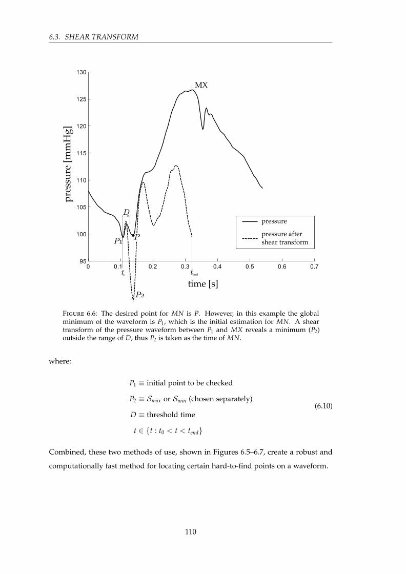
6.3. SHEAR TRANSFORM
Figure 6.6: The desired point for MN is P. However, in this example the globalminimum of the waveform is P1, which is the initial estimation for MN. A sheartransform of the pressure waveform between P1 and MX reveals a minimum (P2)outside the range of D, thus P2 is taken as the time of MN.
where:
P1 ≡ initial point to be checked
P2 ≡ Smax or Smin (chosen separately)
D ≡ threshold time
t ∈ t : t0 < t < tend
(6.10)
Combined, these two methods of use, shown in Figures 6.5–6.7, create a robust and
computationally fast method for locating certain hard-to-find points on a waveform.
110

CHAPTER 6. PROCESSING THE AORTIC AND PULMONARY ARTERY PRESSUREWAVEFORMS
Figure 6.7: This example is the other situation in the process of finding MN toFigure 6.6, i.e. the initial estimation of the global minimum for MN is correct. Here,the minimum of the shear transform from P1 to MX falls within the range of D, thusthe P1 is taken as MN.
6.4 Point location method
The method for finding the points is described in Table 6.1, along with Sections 6.4.1
and 6.4.2. Table 6.1 gives the full method, except for the points DMPG and DN, which
are described in the next two sections, along with a graphical illustration. The graphical
illustrations are the out-working of the method for a representative waveform, and
are intended only to aid the reader in their understanding of the method, and not to
formally describe the method itself. Due to the complexity of the method for the points
DMPG and DN, these two have been described in Table 6.1 only for the simplest, and
most common case, with the full method described in separate sections with relevant
figures.
111

6.4. POINT LOCATION METHOD
Table 6.1: The step by step method for finding the points on Pao and Ppa, as labelledon the right. The graphics beside each step are for illustration only and are not meantto be part of the definition of the method, rather they are to demonstrate the methodin operation on a representative Pao waveform. Note that the methods described herefor DMPG and DN are not complete as these require a more complex method. Referto Sections 6.4.1 and 6.4.2 for the complete method for these two points.
Step Description Example Relevance
Step 1 Find the global maximum Ppa & Pao
Step 2
Find the global minimum, and
check this point with Equa-
tion (6.7), where D = 0.025, t0 =
tP1 , tend = tMX and P2 = Smax
Ppa & Pao
Step 3
For the simplest case, find Smax
between 34 · tMN and tMN, for
the complete method see Sec-
tion 6.4.1
Pao
Step 4
Find Smax between MN and MX,
and check with Equation (6.9)
where D = −0.05 · period, t0 =
tMN, and tend = tP1
Pao
Step 5Find the maximum positive gra-
dient between MN and LSPao
Step 6
The most basic method is to
find Smin between tMX and tend,
which is shown to the right. For
the complete method see Sec-
tion 6.4.2
Ppa & Pao
Step 7Find Smax between MX2 and DN.
MX2 is defined in Equation (6.14)Pao
112
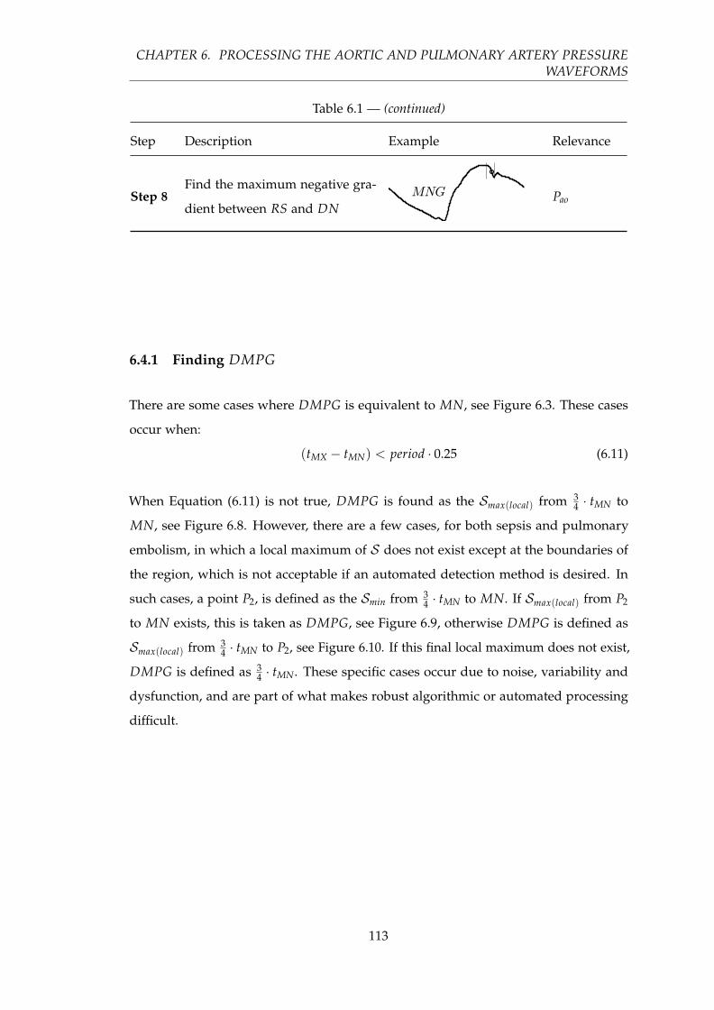
CHAPTER 6. PROCESSING THE AORTIC AND PULMONARY ARTERY PRESSUREWAVEFORMS
Table 6.1 — (continued)
Step Description Example Relevance
Step 8Find the maximum negative gra-
dient between RS and DNPao
6.4.1 Finding DMPG
There are some cases where DMPG is equivalent to MN, see Figure 6.3. These cases
occur when:
(tMX − tMN) < period · 0.25 (6.11)
When Equation (6.11) is not true, DMPG is found as the Smax(local) from 34 · tMN to
MN, see Figure 6.8. However, there are a few cases, for both sepsis and pulmonary
embolism, in which a local maximum of S does not exist except at the boundaries of
the region, which is not acceptable if an automated detection method is desired. In
such cases, a point P2, is defined as the Smin from 34 · tMN to MN. If Smax(local) from P2
to MN exists, this is taken as DMPG, see Figure 6.9, otherwise DMPG is defined as
Smax(local) from 34 · tMN to P2, see Figure 6.10. If this final local maximum does not exist,
DMPG is defined as 34 · tMN. These specific cases occur due to noise, variability and
dysfunction, and are part of what makes robust algorithmic or automated processing
difficult.
113

6.4. POINT LOCATION METHOD
Figure 6.8: A straight forward case for finding DMPG, where P1 of Equation (6.13)exists, thus DMPG ≡ P1.
Figure 6.9: A less common case for finding DMPG, where P1 of Equation (6.13) doesnot exist, but P3 does, thus DMPG ≡ P3.
114
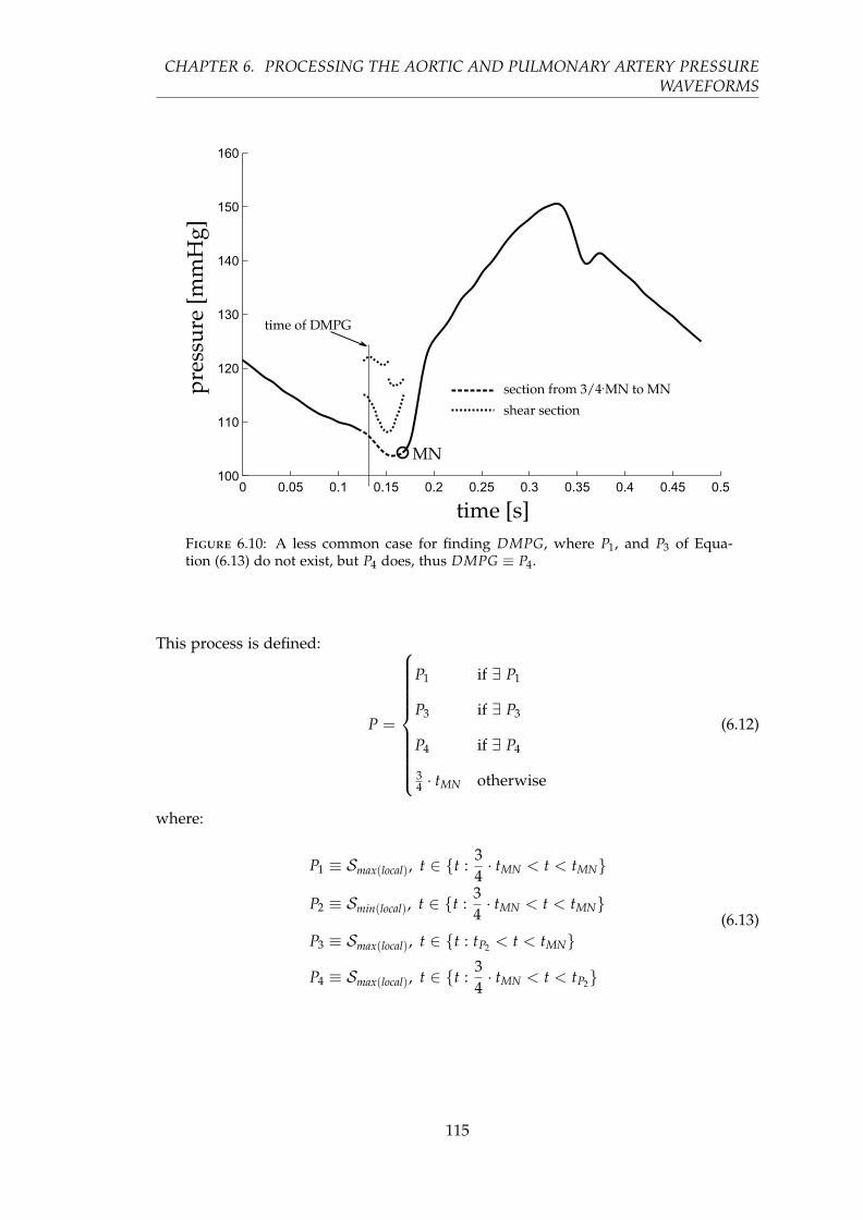
CHAPTER 6. PROCESSING THE AORTIC AND PULMONARY ARTERY PRESSUREWAVEFORMS
Figure 6.10: A less common case for finding DMPG, where P1, and P3 of Equa-tion (6.13) do not exist, but P4 does, thus DMPG ≡ P4.
This process is defined:
P =
P1 if ∃ P1
P3 if ∃ P3
P4 if ∃ P4
34 · tMN otherwise
(6.12)
where:
P1 ≡ Smax(local), t ∈ t :34· tMN < t < tMN
P2 ≡ Smin(local), t ∈ t :34· tMN < t < tMN
P3 ≡ Smax(local), t ∈ t : tP2 < t < tMN
P4 ≡ Smax(local), t ∈ t :34· tMN < t < tP2
(6.13)
115

6.4. POINT LOCATION METHOD
6.4.2 Finding DN
The general approach to find the point DN in Figure 6.3 is to find Smin between tMX
and tend (end of the waveform). However, in a number of cases this approach fails due
to oscillations towards the end of the waveform, as shown in Figure 6.11. In addition,
using only the first local minimum, as would work in Figure 6.11, works in only a
few cases and is therefore not a robust solution. Hence, a more specific algorithm is
required.
Hence, a second maximum point is defined:
MX2 ≡ max point of Pao(t),
t ∈ t : tMN +period
5< t < period
(6.14)
Next, two more intermediate points are defined:
DN1 ≡ (lowest) Smin(local), t ∈ t : tMX2 < t < period (6.15)
DN2 ≡ first Smin(local), t ∈ t : tMX2 < t < period (6.16)
From DN1 and DN2, the real DN is chosen, defined:
DN =
DN1 if (CA ∧ CB) ∨ (CC ∧ CD)
DN2 otherwise(6.17)
where the logical conditions are defined:
CA ≡ DN2 > MX2
CB ≡ (tDN2 − tMX2) < 0.15 · period
CC ≡DN2 − DN1
Pao(tMX)> 0.02
CD ≡ (tDN2 − tMX2) < 0.11 · period
(6.18)
When using a measured Ppa waveform, DN is defined:
DN = DN1 (6.19)
116

CHAPTER 6. PROCESSING THE AORTIC AND PULMONARY ARTERY PRESSUREWAVEFORMS
Figure 6.11: An example of where the first local minimum of the shear transform isthe correct time for the point DN.
6.4.3 Validation Test
The method presented was developed on a set of data from five pigs (51 waveforms) in
which pulmonary embolism was induced (Desaive et al., 2005; Ghuysen et al., 2008).
The method was then independently tested on a further five pigs (37 waveforms) in
which septic shock was induced, and treated with haemofiltration (Lambermont et al.,
2003, 2006). These data sets are therefore effectively development and validation tests.
The points on all waveforms (see Figures 6.3 and 6.4) were identified or checked indi-
vidually by eye. The two gradients (MPG and MNG) were first located through simple
computation, and then individually checked by eye and corrected where necessary.
Due to the nature and location of these points (maximum gradient of a sigmoidal
function), they are the two easiest and most reliable to find algorithmically, and, in fact,
the algorithmic approach is more accurate than hand selection. The two “shoulders”
(LS and RS) were first located through an algorithm developed prior to that which
117

6.5. RESULTS
is described in this chapter, after which each point was individually checked and
corrected. Because there is no formal definition for the location of these “shoulder”
points, it was left to an algorithmic definition. For a validation test this definition is
self fulfilling. However, as LS (RS is used only to aid in finding MNG, and is thus not
included in the validation results) is found as an intermediate step to the estimation of
the time-varying elastance, its full and more formal validation would be the results of
the time-varying estimation, which is not in the scope of this chapter, (see Chapter 7).
All the remaining points were hand selected.
The automated method was applied to the waveforms and the identified points assessed
against the known points for accuracy in time. The use of separate data with different
cardiac dysfunction to design and test the method ensures the robustness of the
validation method.
6.5 Results
For the points MN and DN required when using Ppa (Figure 6.4), the method located
both points in 87 of the 88 waveforms to within the sampling frequency of 200Hz (0.005
sec), missing DN, from one waveform. This missed point is in a waveform at the start
of the third pig of the sepsis cohort and is unique to the data set, both in the measured
time-varying elastance and Ppa, as shown in Figure 6.12, compared to the more typical
Ppa waveform in Figure 6.4. The failure is due to the unusual second peak of Ppa, and
the early decay of the time-varying elastance.
For each Pao waveform, the method locates eight points, MX, MN, DMPG, LS, MPG,
DN, RS, MNG. However, RS and MN are used only to aid the location of other points.
These two points were both located with sufficient accuracy to enable the method to
progress in all 88 waveforms. Results for the other six points are shown in Table 6.2.
Of 528 total points, 519 were found temporally within 1 %, four within 5 %, four within
10 % and one within 20 %.
118

CHAPTER 6. PROCESSING THE AORTIC AND PULMONARY ARTERY PRESSUREWAVEFORMS
Figure 6.12: Ppa alongside the matching time-varying elastance. The automatic oralgorithmic method failed to capture the correct DN point, locating a point too late inthe waveform (circle), the real DN and associated MX are marked by squares.
Table 6.2: Accuracy of the method: number of points grouped by absolute error (of88 total points). ∗ note that the validation of LS here is partially self fulfilling and isincluded here only for completeness.
< 1 % 1–5 % 5–10 % 10–20 %
DMPG 84 1 3 0
MPG 88 0 0 0
LS∗ 86 1 1 0
MX 88 0 0 0
MNG 87 0 0 1
DN 86 2 0 0
TOTAL 519 4 4 1
119

6.6. DISCUSSION
6.6 Discussion
The automated, algorithmic method presented, enables the mapping between aortic
pressure, Pao, pulmonary artery pressure, Ppa, and the ventricular time-varying elastance,
erv(t) and elv(t), by accurately processing the Pao and Ppa waveforms to identify specific
points. Once combined, they provide a useful tool for clinicians to obtain accurate time-
varying elastance waveforms without further invasive or risky sensors or procedures.
There are other ways to locate the points on the pressure waveforms, most notably a
derivative and second derivative method. However, this derivative-based approach
becomes problematic in practice due the noise inherent in the waveforms. The method
that has been developed in this chapter was designed to work with the level of noise
that is typically seen on these measurements, and is therefore more involved than a
simple derivative-based method.
The method presented was robust to the typical and significant variation and noise in
Pao and Ppa waveforms. The method was developed on five pigs in which pulmonary
embolism was induced, and then tested independently with data from another set
of five pigs in which septic shock was induced. The results give confidence that this
method will generalize to a wider set of disease states and to human data.
However, while the results were very good, this research needs further validation on a
wider cohort of pigs and types of dysfunction to further quantify its limits and accuracy.
Direct validation on humans is the ultimate goal. However, the results appear robust,
and justify and enable a wide range of further more in-depth validation studies of both
the method and its potential uses when reconstructing the time-varying elastance for
monitoring and diagnosis.
Clinically, it must be noted that for this method to work, a Swan-Ganz catheter
is assumed. If radial artery pressure was measured instead, there would be more
oscillations in the waveform, potentially requiring modifications. Swan-Ganz catheters
are still used, and this method presented would add value to their use, which is
otherwise sometimes contested (Frazier and Skinner, 2008; Chatterjee, 2009; Cooper
and Doig, 1996).
120

CHAPTER 6. PROCESSING THE AORTIC AND PULMONARY ARTERY PRESSUREWAVEFORMS
The method developed in this chapter shows promise for gaining clinical insight
and improving diagnosis. It can enable clinicians to get more information about the
patient’s current state, without the use of more invasive procedures, as well as beat-
to-beat tracking of this information. This level of detail is far more than is currently
available, does not add addition risk as it requires no further procedures or sensors,
and could potentially lead to better and earlier diagnosis of dysfunction, as well as
better knowledge of treatment responses.
6.7 Summary
This chapter has presented a robust, and potentially dysfunction-independent method
to find the waveform points necessary to use proven methods to non-invasively and
automatically estimate the otherwise unavailable left and right ventricular time-varying
elastances, with accuracy well within measurement error. This capability is enabled
using standard measurements that are already commonly used in an intensive care
setting, thus involving no additional risk to the patient. The results thus justify
prospective validation and extension of these results towards clinical application.
121

Chapter 7
Estimating ventricular time-varying
elastance
In Chapter 6, points were extracted from the aortic and pulmonary artery pressure
waveforms, Pao and Ppa, respectively. The primary purpose is to facilitate the estimation
of the time-varying elastance on a patient-specific basis. This chapter presents the
method of estimating this time-varying elastance using these points. The combination of
Chapters 6 and 7 results in a method to estimate the time-varying elastance waveforms
from measured pressure waveform data that is readily available in an intensive care
setting.
7.1 Introduction
Detailed cardiac energetics are too invasive to measure in an ICU setting. In particular,
such a measurement requires ventricle pressure and volume (Suga, 1971a), and is
therefore not done in practice. However, if the relevant energetics could be captured
using data from a nearby catheter, the clinical potential of such measurements could be
realised. To date, no such method achieves this aim.
This chapter presents a model for estimating the time-varying elastance from observed
ventricular pressure-volume behaviour, to be used in the modelling of broader cardio-
vascular system (Smith, 2004; Starfinger et al., 2008a; Chung et al., 1997; Revie et al.,
2011a,b). This elastance is required by the cardiovascular model of Chapter 3 to deliver
123

7.1. INTRODUCTION
the pressure-volume measurements observed, and thus implicitly contains preload and
afterload information.
Time-varying elastance (TVE) is defined as (Suga and Sagawa, 1974):
e(t) =Pv(t)
Vv(t)−Vd(7.1)
where, Vd is the intercept of the end-systolic pressure-volume relation with the volume
axis (Sagawa, 1981) and Vd = 0 is assumed for simplicity, Pv(t) is the ventricle pressure
and Vv(t) is the ventricle volume. The waveform e(t) is typically normalised to a value
of 1.0 (Suga et al., 1973). As stated in Chapter 5, the model of time-varying elastance
is load-dependent, and does not have a universal shape, even when normalised with
respect to time and value as some have suggested (Suga et al., 1973). More detail and
discussion regarding the TVE see Chapter 5.
Load conditions are diagnostic and thus the model for TVE presented monitors these
changes as the time varying ability of the heart to pump blood. It thus provides
a measure of heart function and energetics (Suga et al., 1973; Senzaki et al., 1996;
Sunagawa et al., 1984).
There have been several attempts to estimate TVE (Guarini et al., 1998; Swamy et al.,
2009; Shishido et al., 2000; Senzaki et al., 1996; Brinke et al., 2010). Most studies present
a method using the TVE to estimate a specific parameter, most commonly end-systolic
elastance (Shishido et al., 2000; Brinke et al., 2010; Senzaki et al., 1996) and ejection
fraction (Swamy et al., 2009). However, their validation is based on these metrics, not
on the resulting TVE waveform, which contains unique clinical information.
This chapter is focused not on the absolute values of the elastance, such as end-systolic
elastance. Rather, the focus is on the shape, and change of shape of the time-varying
waveform within a specific patient as dysfunction occurs and the patient’s state changes.
This intra-patient variability is reflected in the (relative) shape as it evolves over time.
Thus, the patient is their own comparator in this use.
It is unclear how much specific clinical information can be obtained from the TVE
waveform, other than the highly sought-after end-systolic elastance (Burkhoff, 2009),
and a measure of cardiac work (the area under the TVE waveform is analogous to
work done by the ventricle). The absolute value of the work done is lost with the
124

CHAPTER 7. ESTIMATING VENTRICULAR TIME-VARYING ELASTANCE
normalisation of the waveform, but the relative changes to work over time remain. This
point holds true for a constant inotropic state, as the end-systolic elastance will remain
the same. For a varying end-systolic elastance, the relative change in cardiac power
will still be visible to the TVE through the altered shape from an increased heart rate.
Beyond cardiac work, a number of TVE features have been highly correlated to clinically
relevant parameters in a previously developed circulatory model (Starfinger et al., 2007).
Equally, it contains similar information to that of the pressure-volume (PV) loops, which
are known to contain information on cardiac function (Sagawa, 1978) including cardiac
work (Suga, 1990b; Burkhoff and Sagawa, 1986), contractility (Broscheit et al., 2006;
Suga et al., 1973), O2 consumption (Burkhoff and Sagawa, 1986; Suga, 1979a), and
all the states of filling, contraction, ejection and relaxation (Hall and Guyton, 2011).
Overall, the TVE reflects cardiac state, cardiac output or blood volume, and net preload
and afterload, all of which change with different cardiac dysfunction. Hence, the ability
to directly measure TVE, which does not currently exist without significantly invasive
additional testing, should yield clinically useful insight and diagnostically valuable
information. For a more in-depth discussion of the TVE see Chapter 5.
This research is unique in that the end goal is to produce the TVE function in its own
right, validating the TVE waveform on its own accuracy compared to the invasively
and directly measured waveform. This waveform identification is done through the use
of only commonly available metrics in an ICU setting, and thus by being non-invasive,
it is meant that it is no more invasive than traditional care and requires no further
invasive sensors or procedures.
7.2 Methods
7.2.1 Concept
Ventricular time-varying elastance cannot be directly measured without invasive proce-
dures. However, the information contained within the time-varying elastance waveform
can be seen in other parts of the closely intertwined cardiovascular system. There-
fore, with the right knowledge and transformations, that information can be collected
125

7.2. METHODS
and translated into an estimation of a metric (time-varying elastance) that would not
normally be possible to obtain.
The best accessible source of indirect information about time-varying elastance is
directly down-stream of the ventricles, at the aorta and the pulmonary artery. This
location is the first to ‘see’ any results of a change in elastance during systole. Thus,
the aortic and pulmonary artery pressure waveforms (Pao and Ppa, respectively) are
key sources of information, which contain surrounding load conditions, to reconstruct
time-varying elastances. It can be assumed, and seen from the data presented in this
chapter, that the shape of the time-varying elastance is load dependent. For further
discussion on the time-varying elastance’s load dependence, see Chapter 5.
Figure 7.1 shows the overall method of this chapter. Known points on the aortic
pressure waveform are correlated with points on the left ventricle TVE (described in
Section 7.2.4), giving equations that enable estimations of these left ventricle points
from the aortic pressure alone. A function is then used to draw a smooth line through
these estimated points (described in Section 7.2.3) giving a continuous approximation
of the left ventricle TVE. The right ventricle is estimated in a similar way. Known points
from the estimated left ventricle TVE, time values taken from the pulmonary artery
pressure, and the global end-diastolic volume (GEDV) are correlated with points from
the right ventricle TVE, again creating equations used to estimated a continuous right
ventricle TVE. This overview is shown graphically in Figure 7.1.
A total of eight pieces of information, within the four labelled points on time-varying
elastance waveforms, are needed to draw a smooth curve for the estimated time-varying
elastance. These points (MNG, LS, MPG and MX) are shown on the TVE waveforms
in Figure 7.1 and, beside the respective TVE (with the exception of MX as this is always
1) the breakdown and origin of their values are shown. The points on the pressure
waveform required in this method, from Equation (6.1), are shown on the aortic and
pulmonary artery pressure waveforms. The large hollow arrows show the overall flow
of information within the method, while the smaller arrows show the more fine-grained
flow of information.
126

CH
APTER
7.ESTIM
ATIN
GV
ENTR
ICU
LAR
TIME-VA
RYIN
GELA
STAN
CE
Figure 7.1: An overall description of the method presented in this chapter, showing the left and right TVE waveforms with the four pointsrequired to reconstruct them, along with the origin of these values on the pressure waveforms. The large hollow arrows show the general flow ofinformation, while the smaller arrows show more fine-grained flow.
127

7.2. METHODS
A simpler model is shown in Figure 7.2, which visually shows the difference between
the academic side described in this chapter and the potential clinical use of this research.
Figure 7.2: A simple high-level overview of the method within this chapter. It canbe divided into two parts, the first involves the preparation of the correlations frominvasively measured metrics, the second, a clinical method for use in an intensive caresetting.
It should be noted that the two catheter locations (aorta and pulmonary artery) can ‘see’
the ventricles only during systole, inferring that information about the time-varying
elastance can be known only during systole. However, this limitation is not clinically
significant, as time-varying elastance is primarily defined by what happens during
systole, where it is most active. In addition, systole is the period in which blood
is pumped, which is the primary outcome of the time-varying elastance in terms of
clinical relevance. Changes in cardiac elastance due to dysfunction would change this
time-varying elastance, but the clinical significance would be seen in the altered blood
flow.
7.2.2 Animal Data
The method presented was developed on a cohort of nine porcine subjects divided into
two groups. The first group (five subjects) in which pulmonary embolism was induced
(Desaive et al., 2005; Ghuysen et al., 2008). The second group (four subjects) in which
septic shock was induced (Lambermont et al., 2003). Both trials were under the control
of the ethics committee of the medical faculty of Liege, Belgium.
Measurements were taken every 30 minutes. In total, the first group had 51 sets of
measurements across the five pigs, while the septic shock cohort had 34 over four
pigs. For each pig, the following relevant measurements were taken: Pao, Ppa, left and
128

CHAPTER 7. ESTIMATING VENTRICULAR TIME-VARYING ELASTANCE
right ventricle volume (Vlv, Vrv), left and right ventricle pressure (Plv, Prv). Aortic and
pulmonary artery pressure were measured using catheters, while right and left ventricle
pressures and volumes were directly measured using 7F, 12 electrodes conductance
micro manometer tipped catheters.
Left and right time-varying elastances were calculated directly with the respective
pressure and volume waveforms via Equation (7.1), while setting the dead space
volume to zero. GEDV was calculated as the sum of the individual maximum volumes
of the left and right ventricles.
The data contains varying degrees of cardiac dysfunction from healthy to the fully
developed disease state. It thus provides a good test of the presented methods. The use
of two dysfunction states is designed to illustrate the method’s potential robustness, as
well as its potential clinical use.
7.2.3 Waveform construction
The general shape of the time-varying elastance has three main sections: an exponential
rise (A), a shoulder section (B) and an exponential decay (C), as shown in Figure 7.3.
An invasive vena cava occlusion manoeuvre is assumed to be not available and thus
Vd = 0 in Equation (7.1). The time-varying elastance is normalized to 1.0 (Suga et al.,
1973).
The shape of the time-varying elastance waveform is formed from three known locations
on the waveform; time, slope and height of the maximum rising gradient (t1, .x1,x1)
and maximum falling gradient (t3, .x3,x3), (analogous to MPG and MNG respectively
in Figure 7.1), and the height of the waveform’s left shoulder, x2, (analogous to LS, in
Figure 7.1). These are seven of the eight values needed to reproduce the waveforms.
The eighth is the height of the right shoulder (MX, in Figure 7.1) which is always unity.
The seven variable values are found with correlations from points on the Pao and Ppa
waveforms, as described in Section 7.2.4.
129

7.2. METHODS
Figure 7.3: An example of a typical time-varying elastance broken into its mainsections, an exponential rise (A), decay (C) and a near linear section in between (B).
The TVE waveform is assumed to closely fit two exponential functions (one rise and
one decay) joined by a straight line and e(t) is thus defined:
e(t) =
Fα(t) 0 < t < cα
(1−x2)(t−cα)cβ−cα
+ x2 cα < t < cβ
Fβ(t) cβ < t < period
(7.2)
where:
Fi = ai · e−bi(t−ci)2
(7.3)
130

CHAPTER 7. ESTIMATING VENTRICULAR TIME-VARYING ELASTANCE
and the coefficients of Equation (7.3), also seen in Equation (7.2), are fitted for a specific
waveform, and are defined:
aα = x2
bα = − log(x1/x2)
exp(log(−log(x1/x2) · 2 · (x1/ .x1)) · 2)
cα = − log(x1/x2) · 2 · x1 −.x1 · t1.x1
(7.4)
where aβ, bβ and cβ are similarly defined by replacing subscript one with three and
setting x2 = 1.
This waveform model was chosen for its simplicity and shape, requiring a minimal
amount of data to fit the model, while providing a model flexible enough to represent
the real waveform. Due to the nature of the cardiovascular model that uses this
function as an input, see Chapter 3, it is important that this waveform is continuously
differentiable. A comparison of different TVE model shapes can be found in Section 4.5.
From Section 4.5 it can be seen that the cardiovascular model is sensitive to the first
derivative of the TVE model, making any straight line piecewise model less optimal
than the chosen model.
7.2.4 Cardiac Elastance Correlations
The right and left ventricle elastances are constructed using Equations (7.2)–(7.4).
However, the eight values that identify the separate elastances are found in different
ways.
Table 7.1 shows three different types of correlations, the first of which (α) is the
standard correlation used in most statistical analysis. The second two types, β and γ,
are extensions to two and three variables, respectively.
131

7.2. METHODS
Table 7.1: Reconstruction formulae for the three different types of correlations used toestimate the time-varying elastance.
Key Re-construction Formula
α y = mx + c
β y = m1x1 + m2x2 + c
γ y = m1x1 + m2x2 + m3x3 + c
The left time-varying elastance values are relatively straightforward to find, and all use
the standard correlations, α, from Table 7.1. The right time-varying elastance is slightly
harder to estimate, in part because there is no direct downstream access to the right
ventricle similar to that of the left ventricle. This difficulty occurs because only timing
information is taken from Ppa, which can be replaced with electrocardiography (ECG)
and central venous pressure (CVP), as the Ppa waveform is not as commonly measured
in an ICU. This self-imposed limitation makes the method more clinically applicable.
This limitation necessitates other means to estimate the required values on the right
side, which is mostly done through the use of multi-variable correlations involving
GEDV, and the estimated left time-varying elastance. GEDV is closely connected to
the average volume in the right ventricle, and thus serves to add additional scaling.
The specific correlations found between the left and right elastances are shown in
Section 7.3.
7.2.5 Error calculations
The errors of the estimated time-varying elastance waveforms are defined using a
distance metric between the true etrue and estimated eest waveforms, after both wave-
forms have been normalised to the heart rate (producing a waveform confined to a
1x1 box). This normalisation allows the error metric to be consistent in all directions.
This error metric is chosen over a more standard root mean square error (RMSE), to
more accurately reflect the error between the waveforms. Due to the shape of these
waveforms, a RMSE would over emphasise the error due to any slight timing mismatch
132

CHAPTER 7. ESTIMATING VENTRICULAR TIME-VARYING ELASTANCE
in the steep sections of the waveform. The error at each point on the approximated
waveform is thus defined:
δi = mint∈[0,1]
√(ti − t)2 + (eest(ti)− etrue(t))2
, i = 1, . . . N (7.5)
where N is the number of discrete points on the approximated waveform. The error
of the estimated waveforms is represented by a median and a 90th percentile of the
values of δi in Equation (7.5), for both single waveforms and whole cohort errors.
Where multiple waveforms are involved in a single error metric (such as those of the
whole cohort), the δi values are concatenated into a single vector before the median
and percentile errors are calculated. The values of δi in Equation (7.5), geometrically
correspond to the distance from the point (ti, eest(ti)) to the closest point in the curve
(t, etrue(t)), t ∈ [0, 1], as illustrated in Figure 7.4. For practicality of computation, the
real waveform is discretised, such that the number of points is greater than N. Due to
this discretisation the error is over estimated, as the line between the two points is not
the exact normal line of the point on the estimated waveform. This approximation is
chosen over the exact calculation due to the fact that for a given point on the estimated
waveform there is no guarantee that a point exists on the real waveform that is exactly
normal to it.
7.2.6 Analyses
The time-varying elastances were estimated for every measurement taken at 30-minute
intervals during the onset of the porcine cohort’s cardiac dysfunction, in two different
ways. First, using the correlations created with the entire cohort of nine pigs (both
dysfunctions). Second, using the correlations determined from only the five (or four)
pigs from the alternative dysfunction (pulmonary embolism or septic shock). These
estimations were then evaluated against the true time-varying elastance to determine
the error, as defined in Equation (7.5), which is then presented in summary statistics.
133
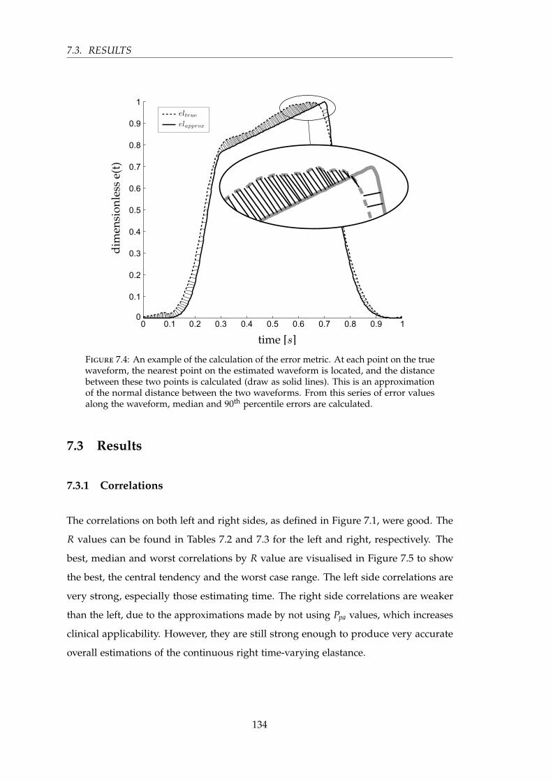
7.3. RESULTS
Figure 7.4: An example of the calculation of the error metric. At each point on the truewaveform, the nearest point on the estimated waveform is located, and the distancebetween these two points is calculated (draw as solid lines). This is an approximationof the normal distance between the two waveforms. From this series of error valuesalong the waveform, median and 90th percentile errors are calculated.
7.3 Results
7.3.1 Correlations
The correlations on both left and right sides, as defined in Figure 7.1, were good. The
R values can be found in Tables 7.2 and 7.3 for the left and right, respectively. The
best, median and worst correlations by R value are visualised in Figure 7.5 to show
the best, the central tendency and the worst case range. The left side correlations are
very strong, especially those estimating time. The right side correlations are weaker
than the left, due to the approximations made by not using Ppa values, which increases
clinical applicability. However, they are still strong enough to produce very accurate
overall estimations of the continuous right time-varying elastance.
134
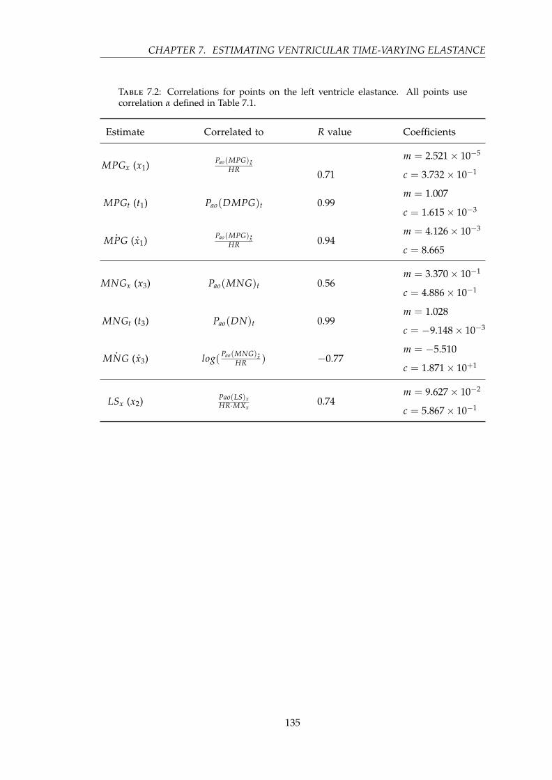
CHAPTER 7. ESTIMATING VENTRICULAR TIME-VARYING ELASTANCE
Table 7.2: Correlations for points on the left ventricle elastance. All points usecorrelation α defined in Table 7.1.
Estimate Correlated to R value Coefficients
MPGx (x1) Pao(MPG).xHR 0.71
m = 2.521× 10⁻⁵
c = 3.732× 10⁻¹
MPGt (t1) Pao(DMPG)t 0.99m = 1.007
c = 1.615× 10⁻³
.MPG ( .x1) Pao(MPG).x
HR 0.94m = 4.126× 10⁻³
c = 8.665
MNGx (x3) Pao(MNG)t 0.56m = 3.370× 10⁻¹
c = 4.886× 10⁻¹
MNGt (t3) Pao(DN)t 0.99m = 1.028
c = −9.148× 10⁻³
.MNG ( .x3) log( Pao(MNG).x
HR ) −0.77m = −5.510
c = 1.871× 10+1
LSx (x2) Pao(LS)xHR·MXx
0.74m = 9.627× 10⁻²
c = 5.867× 10⁻¹
135

7.3.R
ESULTS
Figure 7.5: Three correlations are shown for each of the left (top row), and the right time-varying elastance (bottom row). These three representthe best (left), median (middle) and worst (right) correlations by R value. The median and worst case for the right time-varying elastance aremulti-variable correlations, and therefore only a visualisation, so they cannot be used to read off data in the way a single variable correlationsgraph can.
136
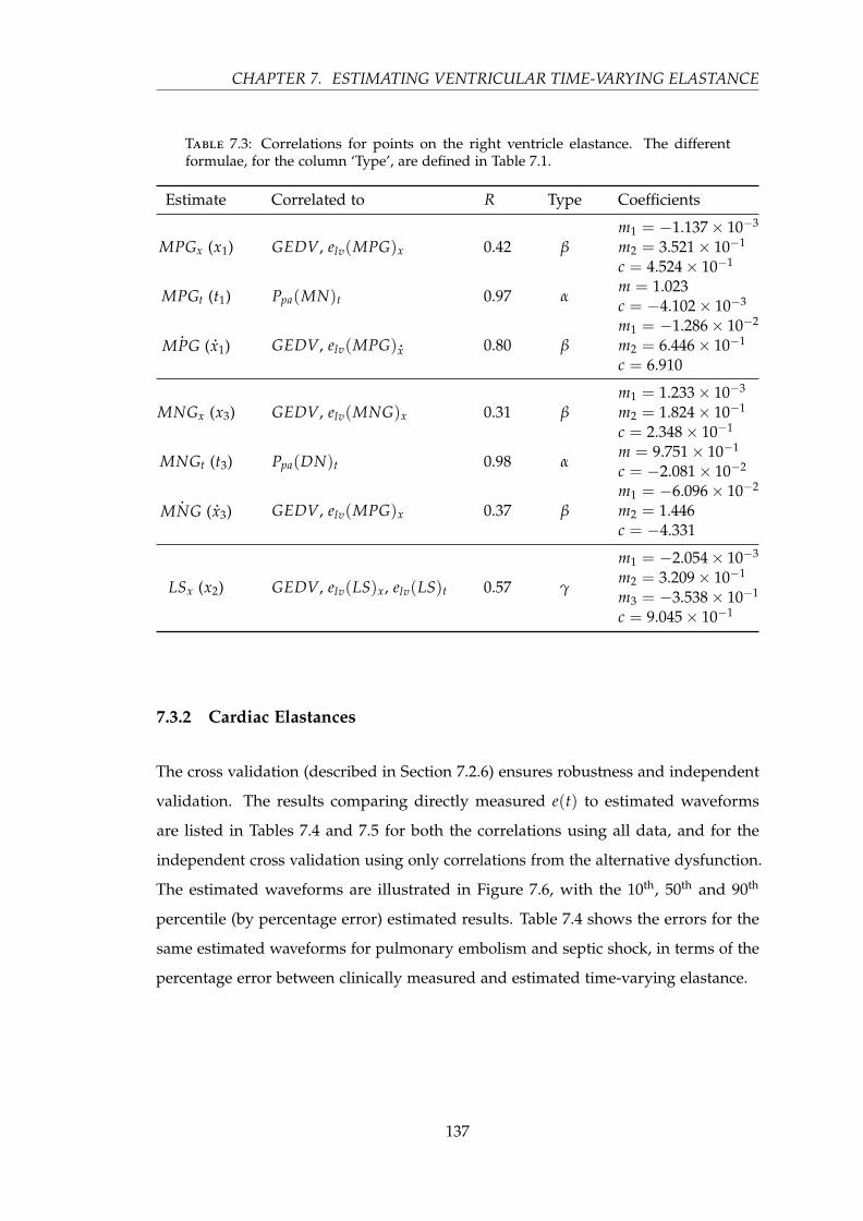
CHAPTER 7. ESTIMATING VENTRICULAR TIME-VARYING ELASTANCE
Table 7.3: Correlations for points on the right ventricle elastance. The differentformulae, for the column ‘Type’, are defined in Table 7.1.
Estimate Correlated to R Type Coefficients
MPGx (x1) GEDV, elv(MPG)x 0.42 βm1 = −1.137× 10⁻³
m2 = 3.521× 10⁻¹
c = 4.524× 10⁻¹
MPGt (t1) Ppa(MN)t 0.97 αm = 1.023c = −4.102× 10⁻³
.MPG ( .x1) GEDV, elv(MPG) .
x 0.80 βm1 = −1.286× 10⁻²
m2 = 6.446× 10⁻¹
c = 6.910
MNGx (x3) GEDV, elv(MNG)x 0.31 βm1 = 1.233× 10⁻³
m2 = 1.824× 10⁻¹
c = 2.348× 10⁻¹
MNGt (t3) Ppa(DN)t 0.98 αm = 9.751× 10⁻¹
c = −2.081× 10⁻²
.MNG ( .x3) GEDV, elv(MPG)x 0.37 β
m1 = −6.096× 10⁻²
m2 = 1.446c = −4.331
LSx (x2) GEDV, elv(LS)x, elv(LS)t 0.57 γ
m1 = −2.054× 10⁻³
m2 = 3.209× 10⁻¹
m3 = −3.538× 10⁻¹
c = 9.045× 10⁻¹
7.3.2 Cardiac Elastances
The cross validation (described in Section 7.2.6) ensures robustness and independent
validation. The results comparing directly measured e(t) to estimated waveforms
are listed in Tables 7.4 and 7.5 for both the correlations using all data, and for the
independent cross validation using only correlations from the alternative dysfunction.
The estimated waveforms are illustrated in Figure 7.6, with the 10th, 50th and 90th
percentile (by percentage error) estimated results. Table 7.4 shows the errors for the
same estimated waveforms for pulmonary embolism and septic shock, in terms of the
percentage error between clinically measured and estimated time-varying elastance.
137
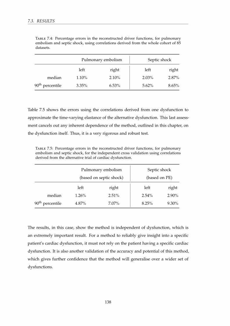
7.3. RESULTS
Table 7.4: Percentage errors in the reconstructed driver functions, for pulmonaryembolism and septic shock, using correlations derived from the whole cohort of 85datasets.
Pulmonary embolism Septic shock
left right left right
median 1.10% 2.10% 2.03% 2.87%
90th percentile 3.35% 6.53% 5.62% 8.65%
Table 7.5 shows the errors using the correlations derived from one dysfunction to
approximate the time-varying elastance of the alternative dysfunction. This last assess-
ment cancels out any inherent dependence of the method, outlined in this chapter, on
the dysfunction itself. Thus, it is a very rigorous and robust test.
Table 7.5: Percentage errors in the reconstructed driver functions, for pulmonaryembolism and septic shock, for the independent cross validation using correlationsderived from the alternative trial of cardiac dysfunction.
Pulmonary embolism Septic shock
(based on septic shock) (based on PE)
left right left right
median 1.26% 2.51% 2.54% 2.90%
90th percentile 4.87% 7.07% 8.25% 9.30%
The results, in this case, show the method is independent of dysfunction, which is
an extremely important result. For a method to reliably give insight into a specific
patient’s cardiac dysfunction, it must not rely on the patient having a specific cardiac
dysfunction. It is also another validation of the accuracy and potential of this method,
which gives further confidence that the method will generalise over a wider set of
dysfunctions.
138

CH
APTER
7.ESTIM
ATIN
GV
ENTR
ICU
LAR
TIME-VA
RYIN
GELA
STAN
CE
Figure 7.6: Results of the estimation of the time-varying elastance alongside the corresponding measured elastance, for both pulmonary embolism(top row) and septic shock (bottom row). For both conditions, the 10th, 50th and 90th percentile cases, by median error, are shown in positions left,middle and right respectively.
139

7.3.R
ESULTS
Figure 7.7: Four reconstructions of the left and right time-varying elastance, from the same pig, as the pulmonary embolism progresses fromhealthy at t = 0 to the end of trial at t = 260.
140

CHAPTER 7. ESTIMATING VENTRICULAR TIME-VARYING ELASTANCE
Figure 7.7 shows four reconstructed time-varying elastances versus the directly mea-
sured time-varying elastances, for pig number 4, at four different times during the
onset of pulmonary embolism. In particular, the dramatic decrease in period at t = 260
min, is captured very well. Overall, the trends and basic shape are captured very well
for the left and reasonably well for the right.
7.4 Discussion
A method for identifying time varying elastance of the left and right ventricles, was
developed that does not require an occlusion manoeuvre to find Vd, and avoids invasive
procedures to measure the left and right ventricle volumes and pressure. These time
varying elastance functions can be used as the input driver function into a lumped
parameter cardiovascular model. The method tracks the main, clinically important time
features on the driver functions, such as the start and end of ejection. This method was
validated on two sets of porcine data, which included multiple measurements of five
pigs in which pulmonary embolism was induced, and four pigs in which septic shock
was induced.
All models are approximations to capture observed physics, and thus all models
offer advantages in understanding these observations as well as the limitations of any
necessary assumptions made.
The approach taken to choose the mapping from the known metrics to the time-varying
elastance, was based both on physiology and accuracy of the resulting time-varying
elastance waveform. Thus, some mappings may not be the most obvious choice based
on purely physiological reasoning. In particular, some of these mappings may appear to
be counterintuitive. For example, although MPG and MNG appear to have symmetry
of meaning in the aortic pressure waveform, this does not transfer into symmetrical
meaning for cardiac energetics, and therefore they do not have symmetry in the chosen
mappings.
The correlations that were used in the reconstructions presented in this chapter are
generally strong. The time-based correlations are especially strong, as seen in, for
example, the two left hand plots (”BEST“) in Figure 7.5, and lead to very good
estimations of the waveform timing. There are also some rather poor correlations, the
141

7.4. DISCUSSION
worst of which predicts the value of the right ventricle TVE at the point MNG. This
correlation has R = 0.31, and a correlation plot that barely shows any correlation at
all. However, the final estimations of the waveform are not very sensitive to this value,
and therefore can produce reasonably accurate waveform estimations from values of
MNGx that are error prone. However, it is important to note that the main results for
this chapter are the errors of the reconstructed waveforms, rather than the presence of
correlations, and these errors were generally small.
There is also a marked difference in the correlation’s R values between the left and right
sides. This is mostly due to not having direct access to the right side of the heart, since
all but the timing of the Ppa waveforms have been neglected. Information about the
right side of the heart is inferred from the left side. Although this results in significantly
lower R-valued correlations (compared to the left), the waveform reconstructions are
still good, with the errors averaging only 5 % higher than the left side for the cross
dysfunction validation.
As would be expected from the correlations in Table 7.2, the timings of the reconstructed
waveforms were very good, capturing the ascending and descending exponential sec-
tions very closely across a large change in cardiac condition, including an approximate
doubling in heart rate. The biggest difference in the real and reconstructed waveforms
usually appeared in the flat section (B of Figure 7.3). This error could be reduced by
using a higher order polynomial or model. However, simulation has shown that this
error is not of significant importance to the existing cardiovascular model (Starfinger
et al., 2008a).
The specific waveform for TVE was chosen as a balance between accuracy and com-
plexity. A model (waveform shape) was needed that provided enough information to
capture the necessary cardiac dynamics, while remaining as simple as possible. The
simplest waveform shape, that could approximate the time-varying elastance, is that
of three, non-zero, straight lines. To fit this model, four points would be required.
Equivalently, two points with associated gradients and two heights — points with free
‘x’ coordinate — which is the currently used data, see Figure 7.1. However, for the same
amount of information and no additional computational complexity, a model of two
exponential curves and one straight line (the chosen model) can be fitted. Furthermore,
this model is continuously differentiable, which can be computationally advantageous
142
CHAPTER 7. ESTIMATING VENTRICULAR TIME-VARYING ELASTANCE
in numerical simulation. This more complex shape provides more accurate results,
without adding complexity to the process of fitting. Beyond this model structure, more
complex models would require additional information to be found from the pressure
waveforms.
Finally, it is worth noting that the overall philosophy and approach of this research
is to add complexity only as required to capture and predict clinical data, and thus
to keep the model as simple as possible. The straight line approach would also have
the benefit of simplifying any semi-analytical solution to speeding up the simulations.
However, until such a semi-analytical approach is developed, the current exponential
formulation is used as it provides more accuracy for non additional cost.
For simplicity of the model, Vd was set to zero, which is a limitation of the current
approach. However, even with this discarded parameter, the model is still able to
capture the necessary dynamics, and provide useful additional information to an ICU
clinician based on the trends observed in TVE shape relative to this assumption. Having
an accurate Vd value in addition would add useful information, but is not identifiable
from the data available without added invasive sensors.
Another limitation of the chapter is the small number (N = 9) of porcine subjects,
although there were a large number (N = 85) of data sets used, and only two dysfunc-
tions. However, this chapter serves as a proof of concept. In particular, the results are
intended to justify the methods and thus a larger, complete prospective validation.
Although this study used the pulmonary artery pressure, the points found in the
pulmonary artery pressure waveform could be estimated using the central venous
pressure and ECG. Thus, there is the potential to construct the driver functions without
any knowledge of the right side of the heart. This option would avoid using pulmonary
artery pressure measurements, which are less commonly available in an ICU than
aortic pressure measurements. This study did not have access to CVP and ECG data
for the porcine cohort so used pulmonary artery pressure instead. Future work will
investigate these clinically relevant extensions to minimise invasiveness, including the
application of the methods within an ICU setting.
143
7.5. SUMMARY
7.5 Summary
This chapter describes a method that has huge clinical potential. Currently, disease
states like pulmonary embolism and septic shock are difficult to diagnose accurately
and reliably due to the lack of useful information accessible to the clinician. With access
to the left and right ventricular time-varying elastance waveforms, more information
can be processed in a meaningful and productive way, resulting in better diagnostic
and treatment decisions. This is achieved through a method that uses only currently
available metrics in the ICU, and thus is no more invasive (no additional risk) than
standard clinical practice.
144

Chapter 8
Clinical diagnostics
This chapter looks at the time-varying elastance and pressure waveforms for their
intrinsic clinical value outside of their use in the cardiovascular model. Three metrics
are estimated that have clinical relevance for the cardiac dysfunctions of pulmonary
embolism and septic shock.
8.1 Introduction
Acute cardiovascular dysfunctions, like pulmonary embolism (PE) and septic shock,
severely alter cardiovascular system (CVS) haemodynamics. These changes can be seen
— through measurements made by catheters placed around the heart — as changes
in pressure and flow, and reflect the dynamic changes in the balance of preload and
afterload, indicating an altered cardiac energetic state (Weber and Janicki, 1979; Ross,
1976). However, to access much of this information, the waveforms from the catheters
need to be processed or modelled in ways beyond what is currently available. Through
such processing, energetic metrics can be obtained that would be far too invasive to
measure directly, offering insight beyond what is normally available.
If more of the cardiac energetic metrics could be captured from the data typically
obtained from catheters already present in an ICU setting. Such an approach would
enable the currently unrealised clinical potential of these catheters to be realised,
adding significant new insight. This chapter presents a method to estimate three of
145

8.2. METHODS
these metrics: afterload, systemic vascular resistance (Rsys), and pulmonary vascular
resistance (Rpul).
These three metrics are useful in the diagnosis of pulmonary embolism, in which
Rpul increases (Goldhaber and Elliott, 2003; Elliott, 1992), and for septic shock where
Rsys commonly decreases (Parrillo et al., 1990; Annane et al., 2005), and is linked, by
definition, to a decrease in afterload. The ability to track these three metrics in real
time, at the bedside, would give valuable non-additionally-invasive information to the
clinician, compared to what is currently available, and potentially decrease the time
taken to reach a diagnosis, increase the reliability of that diagnosis, and ultimately
improve patient outcomes through better management.
8.2 Methods
The overall approach in this study was to gather as much information as possible, from
a proven ventricular time-varying elastance approximations (Stevenson et al., 2012b)
and the aortic pressure waveform, that would yield more information about the current
cardiac dysfunction of the patient. The study was conducted on experimental data
taken from a cohort of nine porcine subjects. These nine subjects were divided into
two groups with five pigs in which pulmonary embolism was induced (Desaive et al.,
2005; Ghuysen et al., 2008). Septic shock was induced in the remaining four pigs, these
were treated with haemofiltration starting at two hours (Lambermont et al., 2003). Both
studies were under the control of the Ethics Committee of the Medical Faculty of Liege,
Belgium.
In all subjects except one, measurements were taken every 30 minutes for the duration
of the trial. The exception was a 60-minute interval for one pig in the septic shock
cohort. For each signal, 10 consecutive heartbeats were recorded and averaged, to
a single heartbeat, and stored as a representative of that waveform, at that time. In
total, 51 heartbeats for the pulmonary embolism group, and 34 for the septic shock
group, were saved. In each case, the following relevant measurements were taken:
aortic pressure (Pao), pulmonary artery pressure (Ppa), left and right ventricle volume
(Vlv, Vrv), and left and right ventricle pressure (Plv, Prv). Both the aortic and pulmonary
146
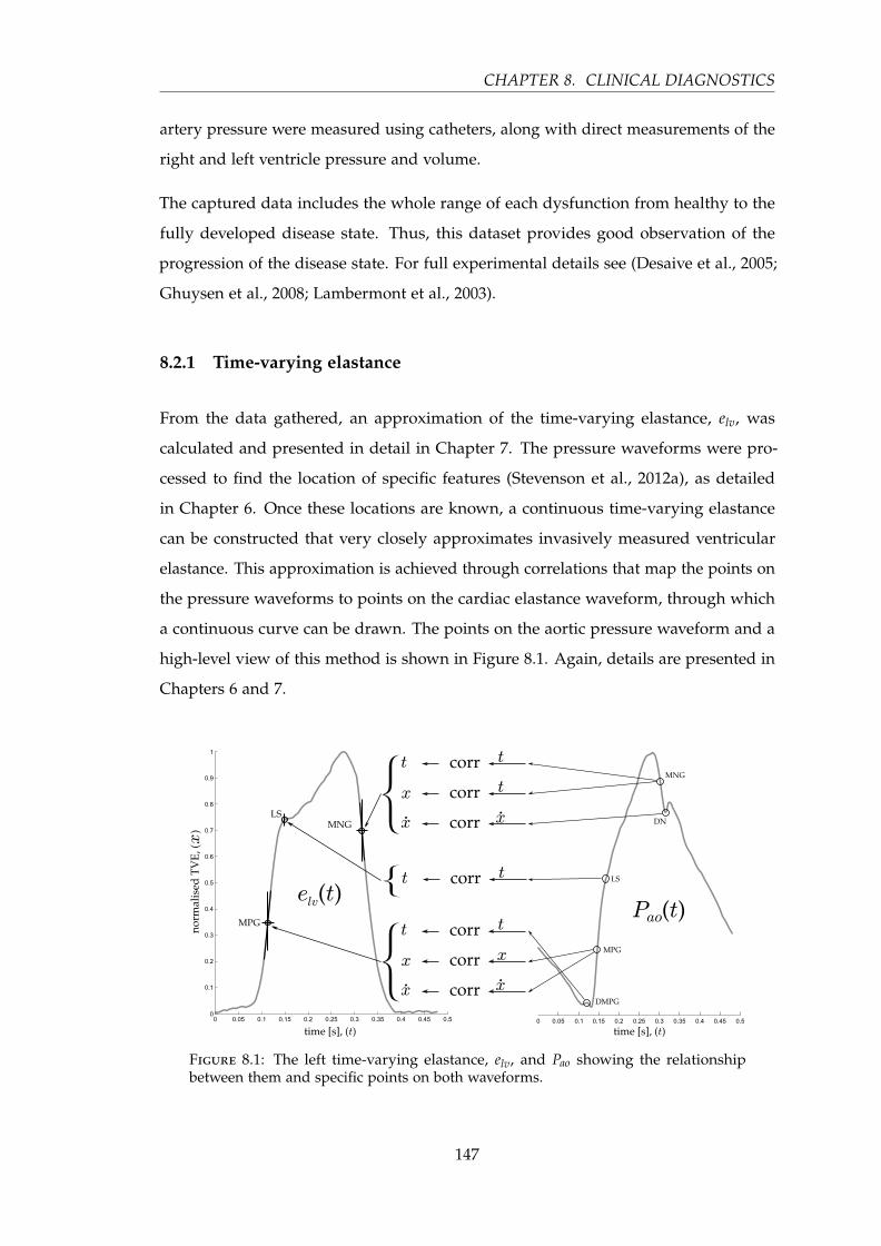
CHAPTER 8. CLINICAL DIAGNOSTICS
artery pressure were measured using catheters, along with direct measurements of the
right and left ventricle pressure and volume.
The captured data includes the whole range of each dysfunction from healthy to the
fully developed disease state. Thus, this dataset provides good observation of the
progression of the disease state. For full experimental details see (Desaive et al., 2005;
Ghuysen et al., 2008; Lambermont et al., 2003).
8.2.1 Time-varying elastance
From the data gathered, an approximation of the time-varying elastance, elv, was
calculated and presented in detail in Chapter 7. The pressure waveforms were pro-
cessed to find the location of specific features (Stevenson et al., 2012a), as detailed
in Chapter 6. Once these locations are known, a continuous time-varying elastance
can be constructed that very closely approximates invasively measured ventricular
elastance. This approximation is achieved through correlations that map the points on
the pressure waveforms to points on the cardiac elastance waveform, through which
a continuous curve can be drawn. The points on the aortic pressure waveform and a
high-level view of this method is shown in Figure 8.1. Again, details are presented in
Chapters 6 and 7.
Figure 8.1: The left time-varying elastance, elv, and Pao showing the relationshipbetween them and specific points on both waveforms.
147
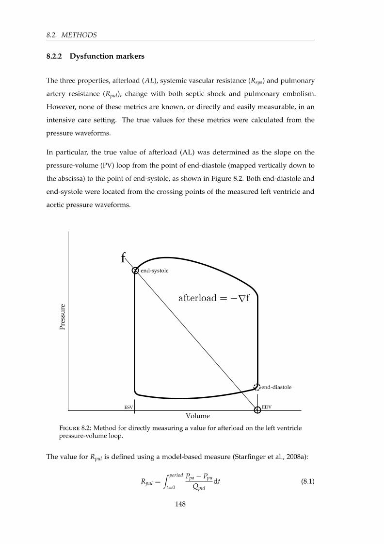
8.2. METHODS
8.2.2 Dysfunction markers
The three properties, afterload (AL), systemic vascular resistance (Rsys) and pulmonary
artery resistance (Rpul), change with both septic shock and pulmonary embolism.
However, none of these metrics are known, or directly and easily measurable, in an
intensive care setting. The true values for these metrics were calculated from the
pressure waveforms.
In particular, the true value of afterload (AL) was determined as the slope on the
pressure-volume (PV) loop from the point of end-diastole (mapped vertically down to
the abscissa) to the point of end-systole, as shown in Figure 8.2. Both end-diastole and
end-systole were located from the crossing points of the measured left ventricle and
aortic pressure waveforms.
Figure 8.2: Method for directly measuring a value for afterload on the left ventriclepressure-volume loop.
The value for Rpul is defined using a model-based measure (Starfinger et al., 2008a):
Rpul =∫ period
t=0
Ppa − Ppu
Qpuldt (8.1)
148
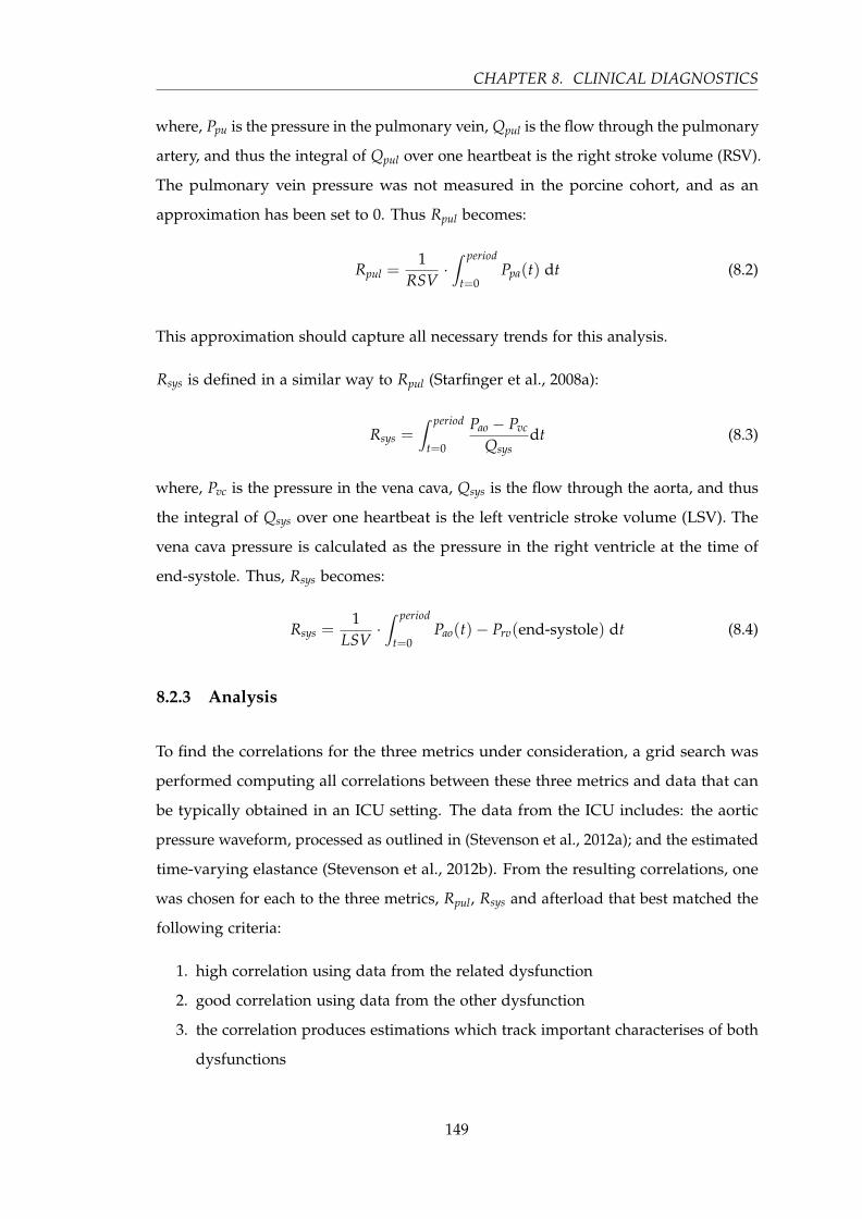
CHAPTER 8. CLINICAL DIAGNOSTICS
where, Ppu is the pressure in the pulmonary vein, Qpul is the flow through the pulmonary
artery, and thus the integral of Qpul over one heartbeat is the right stroke volume (RSV).
The pulmonary vein pressure was not measured in the porcine cohort, and as an
approximation has been set to 0. Thus Rpul becomes:
Rpul =1
RSV·∫ period
t=0Ppa(t) dt (8.2)
This approximation should capture all necessary trends for this analysis.
Rsys is defined in a similar way to Rpul (Starfinger et al., 2008a):
Rsys =∫ period
t=0
Pao − Pvc
Qsysdt (8.3)
where, Pvc is the pressure in the vena cava, Qsys is the flow through the aorta, and thus
the integral of Qsys over one heartbeat is the left ventricle stroke volume (LSV). The
vena cava pressure is calculated as the pressure in the right ventricle at the time of
end-systole. Thus, Rsys becomes:
Rsys =1
LSV·∫ period
t=0Pao(t)− Prv(end-systole) dt (8.4)
8.2.3 Analysis
To find the correlations for the three metrics under consideration, a grid search was
performed computing all correlations between these three metrics and data that can
be typically obtained in an ICU setting. The data from the ICU includes: the aortic
pressure waveform, processed as outlined in (Stevenson et al., 2012a); and the estimated
time-varying elastance (Stevenson et al., 2012b). From the resulting correlations, one
was chosen for each to the three metrics, Rpul, Rsys and afterload that best matched the
following criteria:
1. high correlation using data from the related dysfunction
2. good correlation using data from the other dysfunction
3. the correlation produces estimations which track important characterises of both
dysfunctions
149
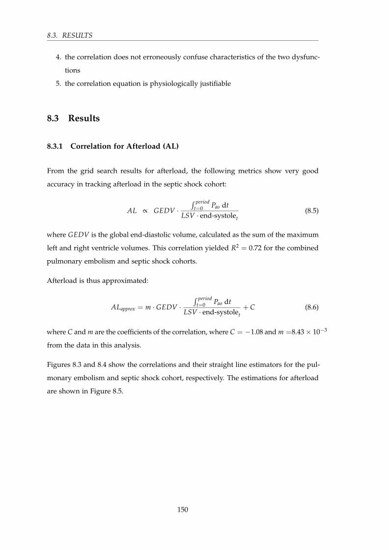
8.3. RESULTS
4. the correlation does not erroneously confuse characteristics of the two dysfunc-
tions
5. the correlation equation is physiologically justifiable
8.3 Results
8.3.1 Correlation for Afterload (AL)
From the grid search results for afterload, the following metrics show very good
accuracy in tracking afterload in the septic shock cohort:
AL ∝ GEDV ·∫ period
t=0 Pao dtLSV · end-systolet
(8.5)
where GEDV is the global end-diastolic volume, calculated as the sum of the maximum
left and right ventricle volumes. This correlation yielded R2 = 0.72 for the combined
pulmonary embolism and septic shock cohorts.
Afterload is thus approximated:
ALapprox = m · GEDV ·∫ period
t=0 Pao dtLSV · end-systolet
+ C (8.6)
where C and m are the coefficients of the correlation, where C = −1.08 and m =8.43× 10⁻³
from the data in this analysis.
Figures 8.3 and 8.4 show the correlations and their straight line estimators for the pul-
monary embolism and septic shock cohort, respectively. The estimations for afterload
are shown in Figure 8.5.
150

CHAPTER 8. CLINICAL DIAGNOSTICS
Figure 8.3: The correlation for estimating afterload, in the septic shock and pulmonaryembolism cohorts separately.
Figure 8.4: The correlation for estimating afterload in the combined septic shock andpulmonary embolism cohorts.
151
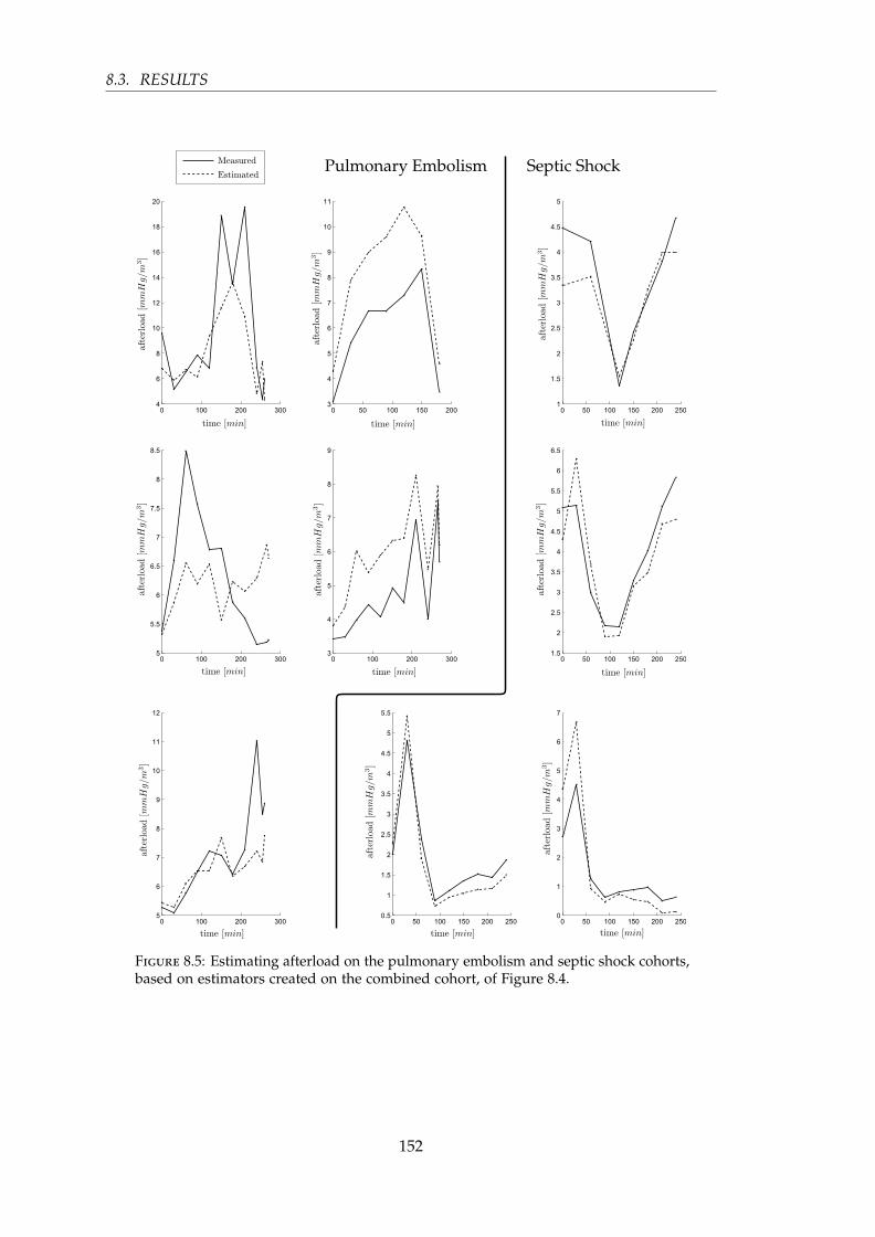
8.3. RESULTS
Figure 8.5: Estimating afterload on the pulmonary embolism and septic shock cohorts,based on estimators created on the combined cohort, of Figure 8.4.
152

CHAPTER 8. CLINICAL DIAGNOSTICS
8.3.2 Correlation for systemic resistance (Rsys)
The correlation that produced the best results for Rsys was:
Rsys ∝ period · Pao(DMPG)
LSV(8.7)
where DMPG is defined in Figure 8.1, where R2 = 0.84 for the combined pulmonary
embolism and septic shock cohorts.
The approximation of Rsys is thus defined:
Rsys,approx = m · period · Pao(DMPG)
LSV+ C (8.8)
where C and m are the coefficients of the correlation, where C = −0.0522 and m = 0.916
for these cohorts.
Figures 8.6 and 8.7 show the correlations and their straight line estimators for the
pulmonary embolism and septic shock cohort, respectively. The estimations for Rsys
are shown in Figure 8.9.
Figure 8.6: The correlation for estimating Rsys, in the septic shock and pulmonaryembolism cohorts separately.
This estimator, for Rsys, can be justified from the CVS model, outlined in Chapter 3.
Equation (8.4) can be further simplified to:
Rsys =t
LSV· (Pao − Prv(end-systole)) (8.9)
153
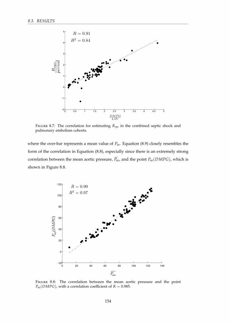
8.3. RESULTS
Figure 8.7: The correlation for estimating Rsys in the combined septic shock andpulmonary embolism cohorts.
where the over-bar represents a mean value of Pao. Equation (8.9) closely resembles the
form of the correlation in Equation (8.8), especially since there is an extremely strong
correlation between the mean aortic pressure, Pao, and the point Pao(DMPG), which is
shown in Figure 8.8.
Figure 8.8: The correlation between the mean aortic pressure and the pointPao(DMPG), with a correlation coefficient of R = 0.985.
154

CHAPTER 8. CLINICAL DIAGNOSTICS
Figure 8.9: Estimating Rsys on the pulmonary embolism and septic shock cohorts,based on estimators created on the combined cohort, of Figure 8.7.
155

8.3. RESULTS
8.3.3 Correlation for pulmonary resistance (Rpul)
The correlation that produced the best results for Rpul was:
Rpul
period2 ∝elv(MPG)
RSV · period(8.10)
where MPG is defined in Figure 8.1, where R2 = 0.536. Thus, the approximation of
Rpul is defined:
Rpul,approx = C1 + C2 ·elv(MPG)
RSV · period(8.11)
where:
C1 = period2 · C
C2 = period2 ·m(8.12)
and C and m are the coefficients of the correlation, where C = 0.29 and m = 44.2 for
these cohorts.
Figures 8.10 and 8.11 show the correlations and their straight-line estimators for the
pulmonary embolism and septic shock cohort respectively. The estimations for Rpul are
shown in Figure 8.12.
Figure 8.10: The correlation for estimating Rpul in the septic shock and pulmonaryembolism cohorts, separately.
156
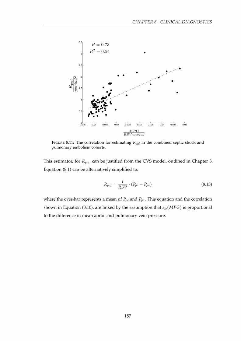
CHAPTER 8. CLINICAL DIAGNOSTICS
Figure 8.11: The correlation for estimating Rpul in the combined septic shock andpulmonary embolism cohorts.
This estimator, for Rpul, can be justified from the CVS model, outlined in Chapter 3.
Equation (8.1) can be alternatively simplified to:
Rpul =t
RSV· (Ppa − Ppu) (8.13)
where the over-bar represents a mean of Ppa and Ppu. This equation and the correlation
shown in Equation (8.10), are linked by the assumption that elv(MPG) is proportional
to the difference in mean aortic and pulmonary vein pressure.
157
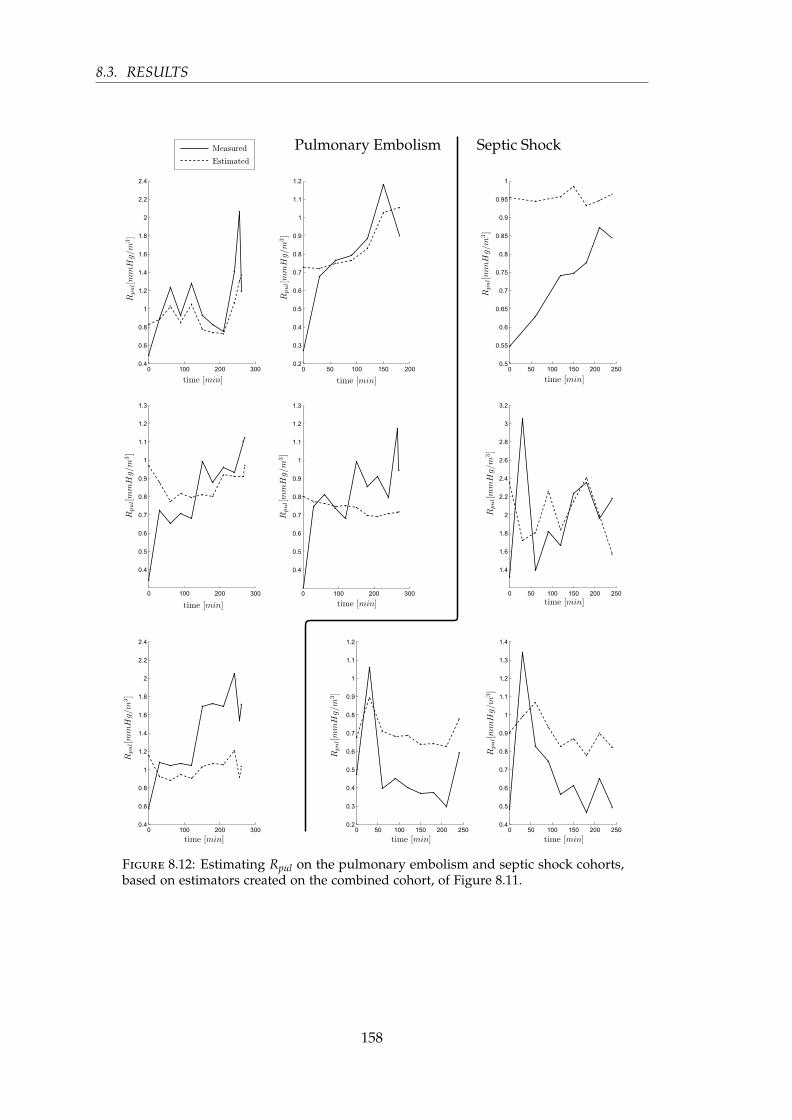
8.3. RESULTS
Figure 8.12: Estimating Rpul on the pulmonary embolism and septic shock cohorts,based on estimators created on the combined cohort, of Figure 8.11.
158

CHAPTER 8. CLINICAL DIAGNOSTICS
8.4 Discussion
The results presented in this chapter, provide good, but not perfect, estimations
of afterload, Rsys and Rpul over a wide range of disease states and their evolution.
The correlations are based on readily available measurements (aortic pressure, stroke
volume and GEDV) and estimates of elastance (elv). They are also generic and applicable
across both cohorts with their different presentation. Thus, errors in the resulting
estimates are acceptable, given overall good results of R2 = 0.72, 0.84 and 0.54, because
these values are not at all available otherwise.
It should be noted that all three correlations require an estimate or measurement of
stroke volume for each side of the heart (RSV and LSV). In most cases, the left and
right stroke volume should be the same or very similar, in which case RSV and LSV
could be replaced with the more generic stroke volume that is often available in the
ICU from PiCCO and similar approaches. However, the subjects in this trial showed
significant differences between the two stroke volumes and thus, for this presentation,
they have been kept separate.
The correlations presented in this chapter were chosen as those that best matched
the most critical dysfunction, while still being able to match the trends for the other
dysfunction. However, there is justification from the clinically validated CVS model
of Chapter 3 as well. In particular, the correlations for Rpul and Rsys can be partially
derived from the model itself.
A distinction can be made between the two disease states from the estimations shown
in Figures 8.5, 8.9 and 8.12. A sharp drop is clearly visible in all the septic shock
subjects in both afterload and Rsys, but importantly, it occurs in none of the pulmonary
embolism subjects. It could therefore be assumed, that if this sharp drop is seen, the
subject has a higher probability of having septic shock, despite potentially similar
outward presentation in terms of reduced cardiac output and stroke volume.
Similarly, for the pulmonary embolism cohort, a steady but significant increase in the
estimated Rpul is observed, while for the septic shock cohort, Rpul averages out to be
steady with a slight decline. These results can be seen in Figure 8.12.
159

8.4. DISCUSSION
The three parameter estimations presented in this chapter are all very useful metrics to
have access to as a clinician, for both diagnosis and management. For example, if Rsys
is tracked in real time, it would enable accurate determination of when vasopressor
therapy should begin, and based on responsiveness to that therapy, Rsys could help
optimise dosage. Importantly, none of these metrics are available currently, without
extensive additional invasive procedures, so this approach would be a major step
forward.
The main effect of these metrics is their relative change over time, and this behaviour is
captured very well in almost all cases. The two exceptions were for the third and fourth
subjects in the pulmonary embolism cohort. For the third subject for afterload, shown
in Figure 8.5 (column 1, row 2), although the estimation in this specific case does not
follow the trend, the estimation will not be confused with sepsis, as afterload does
not fall sharply. Hence, in combination the three metrics are effective and specific in
monitoring and diagnosis. For the fourth subject for Rpul, shown in Figure 8.12 (column
2, row 2), the exception is more troubling. This subject presents in a similar way to
those with septic shock, thus an additional factor must be called upon to distinguish
between pulmonary embolism and septic shock, in this case.
The diagnostic value of this information is seen when comparing the two cardiac
dysfunctions, and the relative trend lines for both parameters. In pulmonary embolism,
Rpul will increase due to the obstruction in the pulmonary artery. However, Rpul also
increases in septic shock, usually at a slower rate. Given the results in this chapter, Rpul
does increase more for pulmonary embolism, but not by a significant margin. It is only
when Rpul is combined with afterload and Rsys, that the distinction can be clearly made
between the two cardiac dysfunctions.
Similarly for the septic shock subjects, both afterload and Rsys show rapid decreases
in the early stages, after which they level off. This recovery is most likely due to the
effects of haemofiltration (Revie et al., 2013; Lambermont et al., 2006). Compared to this
initial drop in afterload and Rsys for septic shock, the metrics for pulmonary embolism
show a gradual but distinct rise, but, most notably, they do not show the initial drop as
seen in septic shock.
A larger cohort would be needed to fully validate this study. However, the results
presented demonstrate the use of non-additionally-invasive procedures to extract useful
160

CHAPTER 8. CLINICAL DIAGNOSTICS
information that would otherwise be unknown to an intensive care clinician. They
may thus increase the value of any catheters that may be present, which are currently
increasingly out of favour as the data they provide cannot be effectively applied.
As discussed earlier, this approach is not without limitations. The differences between
the two dysfunctions studied, namely pulmonary embolism and septic shock, are
distinct in most instances but not all. This lack of global clarity calls for additional
information and characterisations to fully differentiate between the two dysfunctions,
and to achieve potentially more accurate correlations. However, even with perfect
correlations, the resulting data is only as good as the estimations of the CVS model,
which, itself cannot fully distinguish between the two dysfunctions with these metrics
alone.
8.5 Summary
This chapter has presented a method to estimate afterload, systemic vascular resistance
and pulmonary vascular resistance, using measurements that are commonly available in
an intensive care setting without any additional invasive procedures. These estimations
are accurate in their relative trends, and can distinguish between these two common
dysfunctions despite similar initial presentation. Hence, they can, in combination,
provide useful addition information to the diagnosis and management of pulmonary
embolism and septic shock.
In essence, although the presented correlations cannot be relied upon in isolation, they
provide additional information to a clinician. They thus add effective information to
develop an evolving picture of statistical probability for a final diagnosis of cardiac
dysfunction.
161


Chapter 9
Conclusions
This chapter draws together the research presented in this dissertation, including the
motivation and main achievements.
9.1 Background and motivation
The ICU treats the most critically ill patients in the hospital and deals with a diverse
set of cardiovascular and other physiological dysfunctions. The nature of the ICU
means that decisions on diagnosis and treatment are time critical, and often their
accuracy is the difference between life and death. Therefore, it is of utmost importance
that the clinical staff are presented with a full and clear picture of the state of their
patients, including the cardiovascular state, which is troubled by complex interactions
and reflex responses that can mask dysfunction. One method of simplifying the wealth
of information available through monitoring, is to create a computer model of the
patient’s cardiovascular state. Such a model is presented in this research that accurately
represents a specific patient’s cardiovascular state, giving the clinician clear and more
understandable information.
The main thrust of this research is to provide this model with a necessary input
waveform, the time-varying elastance, that would be too invasive to actually measure
in an intensive care unit. The success of the estimation of this waveform resulted in the
use of the time-varying elastance on its own, separate from the cardiovascular model,
to give clinically relevant information. Therefore, this research has achieved two major
163
9.2. MAIN ACHIEVEMENTS
goals: increasing the accuracy of the cardiovascular model through a patient-specific
time-varying elastance waveform, and providing an accurate estimation of the time-
varying elastance for use directly in understanding and tracking the state of a patient’s
heart.
9.2 Main achievements
A small but significant result of this research is the approach developed to process
the noisy and variable measured waveforms for use in the estimation of the time-
varying elastance. Without this method, a real-time estimation of the time-varying
elastance would not have been possible. The method is described in detail in Section 6.3,
and involves a shear transformation of specific sections of the waveform in question,
resulting in the required point becoming a global maximum or minimum of the
transformed shape. In other words, a hard-to-find “shoulder” is transformed into
an easy-to-locate maximum or minimum. This method, along with the other details
mentioned in Chapter 6, allowed for the automation of the accurate location of the
required points. This outcome paved the way to estimate the time-varying elastance in
a real-time algorithmic manner, giving easy access to a valuable source of information,
and an input function to the lumped parameter model of Chapter 3.
The most significant result of this research is the ability to estimate the time-varying
elastance of a specific patient with only the data commonly available in an ICU setting.
This outcome results in additional information relating directly to the energetics
of the heart, with no additional risk beyond standard care practices. There have
been prior attempts to estimate the time-varying elastance, but none have achieved
validation based on the measured time-varying elastance, such as was done in Chapter 7.
Although the estimated waveform is a value-normalised time-varying elastance, it has
been shown that the shape of this waveform is dependant on loading conditions, and
is thus clinically relevant in assessing diagnosis and treatments response, despite the
controversy surrounding this concept.
The implications of having an easily accessible estimation of the time-varying elastance
waveform are numerous. Most significantly, it enables a more accurate simulation
and identification of the patient-specific cardiovascular model presented in Chapters 3
164

CHAPTER 9. CONCLUSIONS
and 4, along with the intrinsic clinical relevance of the waveform shape itself. It
was demonstrated in Chapter 4 that the time-varying elastance input function to the
cardiovascular model and identification process is important. Previous research on
this model has used population waveforms, which inherently neglect patient-specific
energetic information. Using a waveform that accurately resembles the patient’s true
time-varying elastance results in a more accurate identification of the model parameters,
as well as more accurate simulations. Accurately identified parameters are crucial to
using the model to diagnose and track disease state, and thus, having the right time-
varying elastance input allows for more reliable parameters to influence clinicians on
diagnosis and treatment paths, ultimately leading to better patient care and outcomes.
Aside from the cardiovascular model and the implications of a better patient represen-
tation within the model, the time-varying elastance has clinical potential on its own.
This clinical potential was demonstrated in Chapter 8, although more work could be
done to utilise the full depth of information in this waveform. Due to the proximity
and centrality of the time-varying elastance waveform to the cardiovascular system,
and its dependence on loading conditions, it provides a good source of information of
the health of the heart. This information just needs to be unlocked from the waveform
and presented in an understandable and easily accessible way. Chapter 8 started this
process, and clearly shows the potential for much of the information gained from
the full cardiovascular model to be extracted directly from the time-varying elastance
waveform and measured pressure waveforms. This direct extraction bypasses the
computation cost of identifying and simulating the full cardiovascular model, and thus
yields a novel model-based diagnostic tool, useful in its own right.
9.3 Summary
The central premise of this research is the ability to estimate the time-varying elastance
of the left and right ventricles in a patient-specific manner in an ICU environment.
This goal was achieved with very good accuracy, with no additional risk to the patient
beyond standard care practices. It also raises, and at least partially answers, a question
about the importance and relevance of the time-varying elastance itself in the clinical
setting. For the first time, there is now an easily accessible method for estimating the
time-varying elastance in an ICU environment, which should be able to give valuable
165

9.3. SUMMARY
additional information, apart from the cardiovascular model. In this manner, some
variables have been demonstrated to be accessible from this waveform, yielding several
potential new pathways for diagnosis and treatment.
166
Chapter 10
Future Work
This chapter outlines the next steps in this line of research, from further validation and
clinical trials to improved estimation and modelling techniques.
10.1 Further validation
Validation is key to any model or estimation method, and is thus central to the
progression of the research. Specifically, clinical validation, both from animal trials and,
ultimately, human trials.
10.1.1 Trials
A critical step in the future of this research is further validation of all aspects of the time-
varying elastance estimation. The best form of validation requires the measurement of
the true time-varying elastance, and thus must be done through animal trials where
the left and right ventricular pressure and volume are measured. Current data is
from porcine subjects, and further porcine trials over a range of cardiac dysfunctions
would allow for fine tuning of the estimation parameters, and better confidence in the
resulting estimation method.
Furthermore, similar trials on other animals such as goats or dogs would be helpful
to extend the applicability of the model beyond just porcine subjects, resulting in a
more generalised algorithm in the preparation for its use in humans. Direct validation
167
10.1. FURTHER VALIDATION
of the time-varying elastance in humans is currently an unrealisable goal due to
the invasiveness of the required procedures. It is foreseeable that this could change
with improvements in non-invasive procedures for collecting ventricular data, or new
technology. However, until such a time, the only validation that is practically achievable
is indirectly through the performance of models driven by the estimated time-varying
elastance, such as the six-chamber cardiovascular model presented in this research.
Such indirect validation can be achieved on both animals and humans, thus linking
the invasive and direct validation with indirect model performance. Therefore a future
step is to perform human trials, recording the measurements typically taken in the
ICU, over a range of subjects, conditions and condition severities. Due to the nature
of human trials, gathering the number of subjects is a lengthy process but one which
would be hugely beneficial to the overall strengthening of this research.
Humans trials, such as those just mentioned, would not only help to validate the
time-varying elastance, but be instrumental in the further development and validation
of the cardiovascular model as a whole, and thus serve a wider goal and body of
research. Such cardiovascular model validation would help to progress the model
towards clinical usage, which is an overall goal of the research group.
10.1.2 Clinical diagnostics
So far there has not been much attention in the literature to the clinical diagnostic
capability of the time-varying elastance waveform. This is perhaps due to the lack
of availability of such a waveform in a clinical environment, or the controversy over
the universality, or otherwise, of the shape of the normalised time-varying elastance.
However, from this research it is clear that the time-varying elastance is not universal
in its shape, and there exists useful information in the waveform. It just remains to
further develop what has been shown in this research, extracting more information
from the time-varying elastance with better accuracy, and demonstrating and proving
its worth in a clinical setting.
To achieve this, the aforementioned trials would be a prerequisite. This would enable
a large body of data, across various dysfunctions and dysfunction severities, to be
analysed.
168

CHAPTER 10. FUTURE WORK
10.2 Dead space volume
The current model, as presented in the research, assumes that the dead space volume
of the ventricles Vd, is zero. This is not generally the case, and thus will lead to some
inaccuracy in the model. Given the equation for the time-varying elastance, the dead
space volume adjusts the shape of the time-varying elastance, most notably by altering
the height of the left shoulder. This implies that, given sufficient accuracy of the
estimated time-varying elastance, the real dead space volume may, at least in part, be
embedded into the shape of the waveform, and thus could be extracted. This would
lead to greater direct insight into the cardiovascular state of the patient, along with an
improved cardiovascular system model.
10.3 Modelled estimation
10.3.1 CVP and ECG
The porcine data used in this research did not have central venous pressure (CVP) or
ECG recorded. Instead, only timing was used from the pulmonary artery waveform,
Ppa, to future proof the method for an ICU setting, as Ppa is not as commonly available as
other metrics. The timing taken from Ppa can be found on the CVP and ECG waveforms,
and thus the pulmonary artery pressure should not be needed at all, provided CVP
and ECG are known, which are both commonly measured in an ICU. However, because
cohort data with all of these three measurements was not available during this study,
the validation and actual correlations required for this to happen is left as future work.
10.3.2 Time-varying elastance model
At the core of the time-varying elastance concept is an altered Windkessel model,
similar to those used in the passive elastic chambers of the cardiovascular model.
Therefore, direct mathematical models of the time-varying elastance come naturally to
the concept. It would thus seem likely that given the right configuration of a type of
Windkessel model, a more robust time-varying elastance model should be achievable.
169

10.4. CLINICAL INTEGRATION
There are methods in the literature(Aguado-Sierra et al., 2008), which allow for the
estimation of the flow rate, given the aortic pressure. This adds another extremely
rich piece of information to the time-varying elastance model. Flow is also inherently
dependant on loading conditions, thus giving greater insight into the cardiovascular
state. Adding flow to the estimation of time-varying elastance could prove beneficial in
terms of both the accuracy and range of diagnostics capabilities of the final waveform.
10.3.3 Maximal elastance
Currently the estimated time-varying elastance is value-normalised, and thus the
maximal elastance Emax is not known. However, it has been shown that Emax is a useful
predictor of flow-generating capacity of the ventricle (Suga and Sagawa, 1974), and thus
it is conceivable that the reverse could also be possible. Therefore, given the flow, Emax
could be extracted, resulting in the full raw waveform of the time-varying elastance,
along with the much sought-after maximal elastance as a measure of contractility.
Similar to flow and maximal elastance, Suga and Sagawa (1974) showed that stroke
volume is a function of preload, afterload and maximal elastance. Therefore a similar
reversal could take place enhancing an estimation of the maximal elastance as a function
of loading conditions and stroke volume.
10.4 Clinical integration
The final stage of such future research would see relevant methods and information
being taken into clinical settings. Due to the time-sensitive and life-critical decisions
that are made on a daily basis, clinical staff in an ICU setting need all the help they
can get. Therefore, the ultimate goal of the overarching body of research is to integrate
the patient-specific cardiovascular model and time-varying elastance waveforms into
clinical practice. To reach this goal, further validation and trials must be performed to
cement the accuracy, robustness and clinical relevance of the these methods.
170

CHAPTER 10. FUTURE WORK
171

Bibliography
Abramson, N. S.; Wald, K. S.; Grenvik, A. N.; Robinson, D.; and Snyder, J. V. (1980).
”Adverse occurrences in intensive care units”. JAMA : the journal of the American
Medical Association, 244(14), pp. 1582–4.
Agnelli, G.; Becattini, C.; and Kirschstein, T. (2002). ”Thrombolysis vs heparin in the
treatment of pulmonary embolism: a clinical outcome-based meta-analysis”. Archives
of internal medicine, 162(22), pp. 2537–41.
Aguado-Sierra, J.; Alastruey, J.; Wang, J.-J.; Hadjiloizou, N.; Davies, J.; and Parker,
K. H. (2008). ”Separation of the reservoir and wave pressure and velocity from
measurements at an arbitrary location in arteries”. Proceedings of the Institution of
Mechanical Engineers. Part H, Journal of engineering in medicine, 222(4), pp. 403–16.
Al Otair, H.; Chaudhry, M.; Shaikh, S.; and BaHammam, A. (2009). ”Outcome of
patients with pulmonary embolism admitted to the intensive care unit”. Annals of
Thoracic Medicine, 4(1), pp. 13.
Alberti, C.; Brun-Buisson, C.; Burchardi, H.; Martin, C.; Goodman, S.; Artigas, A.;
Sicignano, A.; Palazzo, M.; Moreno, R.; Boulmé, R.; Lepage, E.; and Le Gall, R.
(2002). ”Epidemiology of sepsis and infection in ICU patients from an international
multicentre cohort study”. Intensive care medicine, 28(2), pp. 108–21.
Amoore, J. N.; Santamore, W. P.; Corin, W. J.; and George, D. T. (1992). ”Computer
simulation of the effects of ventricular interdependence on indices of left ventricular
systolic function”. Journal of biomedical engineering, 14(3), pp. 257–62.
Anderson, D. R. (2007). ”Computed Tomographic Pulmonary Angiography vs
Ventilation-Perfusion Lung Scanning in Patients With Suspected Pulmonary Em-
bolism”. JAMA: The Journal of the American Medical Association, 298(23), pp. 2743.
173

BIBLIOGRAPHY
Angus, D. C.; Linde-Zwirble, W. T.; Lidicker, J.; Clermont, G.; Carcillo, J.; and Pinsky,
M. R. (2001). ”Epidemiology of severe sepsis in the United States: analysis of
incidence, outcome, and associated costs of care”. Critical Care Medicine, 29(7), pp.
1303–10.
Annane, D.; Aegerter, P.; Jars-Guincestre, M. C.; and Guidet, B. (2003). ”Current
epidemiology of septic shock: the CUB-Réa Network”. American journal of respiratory
and critical care medicine, 168(2), pp. 165–172.
Annane, D.; Bellissant, E.; and Cavaillon, J.-M. (2005). ”Septic shock”. The Lancet,
365(9453), pp. 63–78.
Annane, D.; Trabold, F.; Sharshar, T.; Jarrin, I.; Blanc, A. S.; Raphael, J. C.; and Gajdos,
P. (1999). ”Inappropriate sympathetic activation at onset of septic shock: a spectral
analysis approach”. American journal of respiratory and critical care medicine, 160(2), pp.
458–465.
Anrep, G. (1912). ”On the part played by the suprarenals in the normal vascular
reactions of the body”. The Journal of physiology, 45(5), pp. 307–17.
Antonini-Canterin, F.; Faggiano, P.; Zanuttini, D.; and Ribichini, F. (1999). ”Is aortic
valve resistance more clinically meaningful than valve area in aortic stenosis?”. Heart,
82(1), pp. 9–10.
Artero, A.; Zaragoza, R.; and Nogueira, J. M. (2012). ”Epidemiology of Severe Sepsis
and Septic Shock”. In Fernandez, R., editor, Severe Sepsis and Septic Shock - Under-
standing a Serious Killer. InTech.
Avanzolini, G.; Barbini, P.; Cappello, A.; and Cevese, A. (1985). ”Time-varying me-
chanical properties of the left ventricle–a computer simulation”. IEEE transactions on
bio-medical engineering, 32(10), pp. 756–63.
Baan, J. and Velde, E. T. (1988). ”Sensitivity of left ventricular end-systolic pressure-
volume relation to type of loading intervention in dogs”. Circulation Research, 62, pp.
1247–58.
Bahloul, M.; Chaari, A.; Kallel, H.; Abid, L.; Hamida, C. B.; Dammak, H.; Rekik, N.;
Mnif, J.; Chelly, H.; and Bouaziz, M. (2010). ”Pulmonary embolism in intensive
174
BIBLIOGRAPHY
care unit: Predictive factors, clinical manifestations and outcome”. Annals of Thoracic
Medicine, 5(2), pp. 97.
Batzel, J. J. and Bachar, M. (2010). ”Modeling the cardiovascular-respiratory control
system: data, model analysis, and parameter estimation”. Acta biotheoretica, 58(4), pp.
369–80.
Berenholtz, S. M.; Pronovost, P. J.; Lipsett, P. A.; Hobson, D.; Earsing, K.; Farley, J. E.;
Milanovich, S.; Garrett-Mayer, E.; Winters, B. D.; Rubin, H. R.; Dorman, T.; and Perl,
T. M. (2004). ”Eliminating catheter-related bloodstream infections in the intensive
care unit”. Critical care medicine, 32(10), pp. 2014–20.
Bermejo, J.; García-Fernández, M. A.; Torrecilla, E. G.; Bueno, H.; Moreno, M. M.;
San Román, D.; and Delcán, J. L. (1996). ”Effects of dobutamine on Doppler echocar-
diographic indexes of aortic stenosis”. Journal of the American College of Cardiology,
28(5), pp. 1206–13.
Beyar, R.; Hausknecht, M. J.; Halperin, H. R.; Yin, F. C.; and Weisfeldt, M. L. (1987).
”Interaction between cardiac chambers and thoracic pressure in intact circulation”.
American Journal of Physiology, 253(5 Pt 2), pp. H1240–H1252.
Binanay, C.; Califf, R. M.; Hasselblad, V.; O’Connor, C. M.; Shah, M. R.; Sopko, G.;
Stevenson, L. W.; Francis, G. S.; Leier, C. V.; and Miller, L. W. (2005). ”Evaluation
study of congestive heart failure and pulmonary artery catheterization effectiveness:
the ESCAPE trial”. JAMA : the journal of the American Medical Association, 294(13), pp.
1625–33.
Blais, C.; Pibarot, P.; Dumesnil, J. G.; Garcia, D.; Chen, D.; and Durand, L. G. (2001).
”Comparison of valve resistance with effective orifice area regarding flow depen-
dence”. The American journal of cardiology, 88(1), pp. 45–52.
Blitz, L. R. and Herrmann, H. C. (1996). ”Hemodynamic assessment of patients with
low-flow, low-gradient valvular aortic stenosis”. The American journal of cardiology,
78(6), pp. 657–61.
Bone, R. C.; Balk, R. A.; Cerra, F. B.; Dellinger, R. P.; Fein, A. M.; Knaus, W. A.;
Schein, R. M.; and Sibbald, W. J. (1992). ”Definitions for sepsis and organ failure and
guidelines for the use of innovative therapies in sepsis. The ACCP/SCCM Consensus
175

BIBLIOGRAPHY
Conference Committee. American College of Chest Physicians/Society of Critical
Care Medicine”. Chest, 101(6), pp. 1644–55.
Bouman, C. (2007). ”High-Volume Hemofiltration as Adjunctive Therapy for Sepsis
and Systemic Inflammatory Response Syndrome: Background, Definition and a
Descriptive Analysis of Animal and Human Studies”. Advances in Sepsis, 6(2), pp.
47–57.
Braunwald, E. (1976). Mechanisms of contraction of the normal and failing heart. Little,
Brown, Boston, 2nd editio edition.
Brinke, E. A.; Klautz, R. J.; Verwey, H. F.; Wall, E. E.; Dion, R. A.; and Steendijk, P.
(2010). ”Single-beat estimation of the left ventricular end-systolic pressure-volume
relationship in patients with heart failure”. Acta Physiologica (Oxf), 198(1), pp. 37–46.
Broscheit, J. A.; Weidemann, F.; Strotmann, J.; Steendijk, P.; Karle, H.; Roewer, N.;
and Greim, C. A. (2006). ”Time-varying elastance concept applied to the relation
of carotid arterial flow velocity and ventricular area”. Journal af Cardiothoracic and
Vascular Anesthesia, 20(3), pp. 340–6.
Burkhoff, D. (2002). Mechanical properties of the heart and its interaction with the vascular
system. Course Material, Columbia University, New York, USA.
Burkhoff, D. (2009). ”Chasing the Elusive Pressure-Volume Relationship”. Journal of the
American College of Cardiology. Cardiovascular Imaging, 2, pp. 1282–4.
Burkhoff, D.; De Tombe, P. P.; and Hunter, W. C. (1993). ”Impact of ejection on mag-
nitude and time course of ventricular pressure-generating capacity”. The American
journal of physiology, 265(3 Pt 2), pp. H899–909.
Burkhoff, D.; Mirsky, I.; and Suga, H. (2005). ”Assessment of systolic and diastolic
ventricular properties via pressure-volume analysis: a guide for clinical, translational,
and basic researchers”. American journal of physiology. Heart and circulatory physiology,
289(2), pp. H501–12.
Burkhoff, D. and Sagawa, K. (1986). ”Ventricular efficiency predicted by an analytical
model”. American Journal of Physiology, 250(6 Pt 2), pp. R1021–7.
176

BIBLIOGRAPHY
Burkhoff, D.; Sugiura, S.; Yue, D. T.; and Sagawa, K. (1987). ”Contractility-dependent
curvilinearity of end-systolic pressure-volume relations”. American Journal of Physiol-
ogy, 252(6 Pt 2), pp. H1218–27.
Burkhoff, D. and Tyberg, J. V. (1993). ”Why does pulmonary venous pressure rise after
onset of LV dysfunction: a theoretical analysis”. The American journal of physiology,
265(5 Pt 2), pp. H1819–28.
Calvin, J. E.; Driedger, A. A.; and Sibbald, W. J. (1981). ”An assessment of myocardial
function in human sepsis utilizing ECG gated cardiac scintigraphy”. Chest, 80(5), pp.
579–86.
Campbell, K. B.; Simpson, A. M.; Campbell, S. G.; Granzier, H. L.; and Slinker,
B. K. (2008). ”Dynamic left ventricular elastance: a model for integrating cardiac
muscle contraction into ventricular pressure-volume relationships”. Journal of applied
physiology (Bethesda, Md. : 1985), 104(4), pp. 958–75.
Casale, P. N.; Palacios, I. F.; Abascal, V. M.; Harrell, L.; Davidoff, R.; Weyman, A. E.;
and Fifer, M. A. (1992). ”Effects of dobutamine on Gorlin and continuity equation
valve areas and valve resistance in valvular aortic stenosis”. The American journal of
cardiology, 70(13), pp. 1175–9.
Challoner, D. R. (1968). ”Respiration in myocardium”. Nature, 217(5123), pp. 78–9.
Chase, J. G.; Shaw, G.; Le Compte, A.; Lonergan, T.; Willacy, M.; Wong, X.-W.; Lin,
J.; Lotz, T.; Lee, D.; and Hann, C. (2008). ”Implementation and evaluation of the
SPRINT protocol for tight glycaemic control in critically ill patients: a clinical practice
change”. Critical care (London, England), 12(2), pp. R49.
Chatterjee, K. (2009). ”The Swan-Ganz Catheters: Past, Present, and Future”. Circulation,
119, pp. 147–152.
Chen, C. H.; Nevo, E.; Fetics, B.; Pak, P. H.; Yin, F. C.; Maughan, W. L.; and Kass,
D. A. (1997). ”Estimation of central aortic pressure waveform by mathematical
transformation of radial tonometry pressure. Validation of generalized transfer
function”. Circulation, 95(7), pp. 1827–36.
177

BIBLIOGRAPHY
Chung, D. C.; Niranjan, S. C.; Clark, J.; Bidani, A.; Johnston, W. E.; Zwischenberger,
J. B.; and Traber, D. L. (1997). ”A dynamic model of ventricular interaction and
pericardial influence”. American Journal of Physiology, 272(6 Pt 2), pp. H2942–62.
Claessens, T. E.; Georgakopoulos, D.; Afanasyeva, M.; Vermeersch, S. J.; Millar, H. D.;
Stergiopulos, N.; Westerhof, N.; Verdonck, P. R.; and Segers, P. (2006). ”Nonlinear
isochrones in murine left ventricular pressure-volume loops: how well does the time-
varying elastance concept hold?”. American journal of physiology. Heart and circulatory
physiology, 290(4), pp. H1474–83.
Cloud, G. C.; Rajkumar, C.; Kooner, J.; Cooke, J.; and Bulpitt, C. J. (2003). ”Estimation of
central aortic pressure by SphygmoCor requires intra-arterial peripheral pressures”.
Clinical science (London, England : 1979), 105(2), pp. 219–25.
Cole, L.; Bellomo, R.; Journois, D.; Davenport, P.; Baldwin, I.; and Tipping, P. (2001).
”High-volume haemofiltration in human septic shock”. Intensive care medicine, 27(6),
pp. 978–86.
Cooper, A. B. and Doig, G. S. S. (1996). ”Pulmonary artery catheters in the critically
ill”. Critical Care Medicine, 12, pp. 777–94.
Cooper, G. (1990). ”Load and length regulation of cardiac energetics”. Annual review of
physiology, 52, pp. 505–22.
Cornejo, R.; Downey, P.; Castro, R.; Romero, C.; Regueira, T.; Vega, J.; Castillo, L.;
Andresen, M.; Dougnac, A.; Bugedo, G.; and Hernandez, G. (2006). ”High-volume
hemofiltration as salvage therapy in severe hyperdynamic septic shock”. Intensive
care medicine, 32(5), pp. 713–722.
Corrigan, J. J. J.; Ray, W. L.; and May, N. (1968). ”Changes in the blood coagulation
system associated with septicemia”. The New England journal of medicine, 279(16), pp.
851–856.
Covell, J. W.; Taylor, R. R.; Sonnenblick, E. H.; and Ross, J. (1975). ”Series elasticity in
the intact heart. Evidence for the application of the Hill model for muscle to the intact
left ventricle”. Pflügers Archiv : European journal of physiology, 357(3-4), pp. 225–36.
178
BIBLIOGRAPHY
De Backer, D.; Creteur, J.; Preiser, J.-C.; Dubois, M.-J.; and Vincent, J.-L. (2002). ”Mi-
crovascular blood flow is altered in patients with sepsis”. American journal of respira-
tory and critical care medicine, 166(1), pp. 98–104.
Dellinger, R. P.; Levy, M. M.; Carlet, J. M.; Bion, J.; Parker, M. M.; Jaeschke, R.; Reinhart,
K.; Angus, D. C.; Brun-Buisson, C.; Beale, R.; Calandra, T.; Dhainaut, J.-F.; Gerlach,
H.; Harvey, M.; Marini, J. J.; Marshall, J.; Ranieri, M.; Ramsay, G.; Sevransky, J.;
Thompson, B. T.; Townsend, S.; Vender, J. S.; Zimmerman, J. L.; and Vincent, J.-L.
(2008). ”Surviving Sepsis Campaign: international guidelines for management of
severe sepsis and septic shock: 2008”. Intensive care medicine, 34(1), pp. 17–60.
Desaive, T.; Dutron, S.; Lambermont, B.; Kolh, P.; Hann, C. E.; Chase, J. G.; Dauby, P. C.;
and Ghuysen, A. (2005). ”Close-loop model of the cardiovascular system including
ventricular interaction and valve dynamics: application to pulmonary embolism”.
12th Intl Conference on Biomedical Engineering (ICBME).
Desaive, T.; Ghuysen, A.; Lambermont, B.; Kolh, P.; Dauby, P. C.; Starfinger, C.;
Hann, C. E.; Chase, J. G.; and Shaw, G. M. (2008). ”Cardiovascular Modelling and
Identification in Septic Shock - Experimental validation”. In Proceedings of the 17th
IFAC World Congress, Seoul, Korea.
Di Nisio, M.; Squizzato, A.; Rutjes, A. W. S.; Büller, H. R.; Zwinderman, A. H.; and
Bossuyt, P. M. M. (2007). ”Diagnostic accuracy of D-dimer test for exclusion of
venous thromboembolism: a systematic review”. Journal of thrombosis and haemostasis:
JTH, 5(2), pp. 296–304.
Dombrovskiy, V. Y.; Martin, A. A.; Sunderram, J.; and Paz, H. L. (2007). ”Rapid increase
in hospitalization and mortality rates for severe sepsis in the United States: a trend
analysis from 1993 to 2003”. Critical care medicine, 35(5), pp. 1244–50.
Donchin, Y.; Gopher, D.; Olin, M.; Badihi, Y.; Biesky, M.; Sprung, C. L.; Pizov, R.; and
Cotev, S. (1995). ”A look into the nature and causes of human errors in the intensive
care unit”. Critical care medicine, 23(2), pp. 294–300.
Douketis, J. D. (2001). ”Prognosis in pulmonary embolism”. Current opinion in pul-
monary medicine, 7(5), pp. 354–9.
Elliott, C. G. (1992). ”Pulmonary physiology during pulmonary embolism”. Chest,
101(4 Suppl), pp. 163S–71S.
179

BIBLIOGRAPHY
Evans, A.; Shaw, G. M.; Le Compte, A.; Tan, C.-S.; Ward, L.; Steel, J.; Pretty, C. G.;
Pfeifer, L.; Penning, S.; Suhaimi, F.; Signal, M.; Desaive, T.; and Chase, J. G. (2011).
”Pilot proof of concept clinical trials of Stochastic Targeted (STAR) glycemic control”.
Annals of intensive care, 1, pp. 38.
Evans, C. L. and Matsuoka, Y. (1915). ”The effect of various mechanical conditions
on the gaseous metabolism and efficiency of the mammalian heart”. The Journal of
physiology, 49(5), pp. 378–405.
Fogel, M. A.; Weinberg, P. M.; Gupta, K. B.; Rychik, J.; Hubbard, A.; Hoffman, E. A.; and
Haselgrove, J. (1998). ”Mechanics of the single left ventricle: a study in ventricular-
ventricular interaction II”. Circulation, 98(4), pp. 330–8.
Fogliardi, R.; Di Donfrancesco, M.; and Burattini, R. (1996). ”Comparison of linear
and nonlinear formulations of the three-element windkessel model”. The American
journal of physiology, 271(6 Pt 2), pp. H2661–8.
Ford, L. E.; Feldman, T.; and Carroll, J. D. (1994). ”Valve resistance”. Circulation, 89(2),
pp. 893–5.
Ford, L. E.; Feldman, T.; Chiu, Y. C.; and Carroll, J. D. (1990). ”Hemodynamic resistance
as a measure of functional impairment in aortic valvular stenosis”. Circulation research,
66(1), pp. 1–7.
Frank, O. (1895). Zur Dynamik des Herzmuskels.. Druck v. R. Oldenbourg.
Frank, O. (1899). ”Die grundform des arteriellen pulses, Erste Abhandlung, Mathema-
tische Analyse”. Z Biol, 37, pp. 483–526.
Frazier, S. K. and Skinner, G. J. (2008). ”Pulmonary artery catheters: state of the
controversy”. Journal of Cardiovascular Nursing, 23, pp. 113–21.
Fung, Y. C. (1993). Biomechanics: Mechanical Properties of Living Tissues, Second Edition.
Springer.
Gan, C. T.; Lankhaar, J. W.; Marcus, J. T.; Westerhof, N.; Marques, K. M.; Bronzwaer,
J. G.; Boonstra, A.; Postmus, P. E.; and Vonk-Noordegraaf, A. (2006). ”Impaired left
ventricular filling due to right-to-left ventricular interaction in patients with pul-
monary arterial hypertension”. American Journal of Physiology. Heart and Circulatory
Physiology, 290(4), pp. H1528–33.
180

BIBLIOGRAPHY
Ganz, W.; Donoso, R.; Marcus, H. S.; Forrester, J. S.; and Swan, H. J. (1971). ”A
new technique for measurement of cardiac output by thermodilution in man”. The
American journal of cardiology, 27(4), pp. 392–6.
Georgakopoulos, D.; Mitzner, W. A.; Chen, C. H.; Byrne, B. J.; Millar, H. D.; Hare, J. M.;
and Kass, D. A. (1998). ”In vivo murine left ventricular pressure-volume relations
by miniaturized conductance micromanometry”. The American journal of physiology,
274(4 Pt 2), pp. H1416–22.
Ghuysen, A.; Lambermont, B.; Kolh, P.; Tchana-Sato, V.; Magis, D.; Gerard, P.; Mom-
mens, V.; Janssen, N.; Desaive, T.; and D’Orio, V. (2008). ”Alteration of right
ventricular-pulmonary vascular coupling in a porcine model of progressive pressure
overloading”. Shock, 29(2), pp. 197–204.
Gibbs, C. L. and Chapman, J. B. (1985). ”Cardiac mechanics and energetics: chemome-
chanical transduction in cardiac muscle”. The American journal of physiology, 249(2 Pt
2), pp. H199–206.
Goldhaber, S. Z. (2002). ”Echocardiography in the management of pulmonary em-
bolism”. Annals of internal medicine, 136(9), pp. 691–700.
Goldhaber, S. Z. and Elliott, C. G. (2003). ”Acute pulmonary embolism: part I: epidemi-
ology, pathophysiology, and diagnosis”. Circulation, 108(22), pp. 2726–9.
Goldhaber, S. Z.; Visani, L.; and De Rosa, M. (1999). ”Acute pulmonary embolism:
clinical outcomes in the International Cooperative Pulmonary Embolism Registry
(ICOPER)”. Lancet, 353(9162), pp. 1386–9.
Greenberg, S. B.; Murphy, G. S.; and Vender, J. S. (2009). ”Current use of the pulmonary
artery catheter”. Current opinion in critical care, 15(3), pp. 249–53.
Grenvik, A.; Ayres, S. M.; and Holbrook, P. R. (1989). Textbook of Critical Care. W.B.
Saunders Company, Philadelphia, 2nd edition.
Groot, M. R.; van Marwijk Kooy, M.; Pouwels, J. G.; Engelage, A. H.; Kuipers, B. F.; and
Büller, H. R. (1999). ”The use of a rapid D-dimer blood test in the diagnostic work-up
for pulmonary embolism: a management study”. Thrombosis and haemostasis, 82(6),
pp. 1588–92.
181

BIBLIOGRAPHY
Guarini, M.; Urzúa, J.; Cipriano, A.; and González, W. (1998). ”Estimation of caridac
function from computer analysis of the arterial pressure waveform”. IEEE Transactions
on Biomedical Engineering, 45(12), pp. 1420–8.
Hall, J. E. and Guyton, A. C. (2011). Guyton and Hall Textbook of Medical Physiology.
Elsevier Health Sciences.
Hann, C. E.; Chase, J. G.; and Shaw, G. M. (2005). ”Efficient implementation of non-
linear valve law and ventricular interaction dynamics in the minimal cardiac model”.
Computer Methods and Programs in Biomedicine, 80(1), pp. 65–74.
Hayashi, K.; Shigemi, K.; Shishido, T.; Sugimachi, M.; and Sunagawa, K. (2000). ”Single-
beat estimation of ventricular end-systolic elastance-effective arterial elastance as
an index of ventricular mechanoenergetic performance”. Anesthesiology, 92(6), pp.
1769–76.
Heidenreich, P. A.; Trogdon, J. G.; Khavjou, O. A.; Butler, J.; Dracup, K.; Ezekowitz,
M. D.; Finkelstein, E. A.; Hong, Y.; Johnston, S. C.; Khera, A.; Lloyd-Jones, D. M.;
Nelson, S. A.; Nichol, G.; Orenstein, D.; Wilson, P. W. F.; and Woo, Y. J. (2011).
”Forecasting the Future of Cardiovascular Disease in the United States A Policy
Statement From the American Heart Association”. Circulation, 123(8), pp. 933–44.
Helmholtz, H. (1845). ”Ueber den Stoffverbrauch bei der Muskelaktion”. Mueller’s Arch
Anal Phyiol, pages 72–83.
Helmholtz, H. (1848). ”Ueber die warmeentwicklung der muskelaction”. Mueller’s
Arch Anal Phyiol, pages 144–64.
Hope, S. A.; Tay, D. B.; Meredith, I. T.; and Cameron, J. D. (2004). ”Use of arterial
transfer functions for the derivation of central aortic waveform characteristics in
subjects with type 2 diabetes and cardiovascular disease”. Diabetes care, 27(3), pp.
746–51.
Hosepud, J. D. and Greenberg, B. H. (2007). Congestive Heart Failure. Lippincott
Williams & Wilkins, Philadelphia.
Hunter, W. C.; Janicki, J. S.; Weber, K. T.; and Noordergraaf, A. (1979). ”Flow-pulse
response: a new method for the characterization of ventricular mechanics”. The
American journal of physiology, 237(3), pp. H282–92.
182

BIBLIOGRAPHY
Hunter, W. C.; Janicki, J. S.; Weber, K. T.; and Noordergraaf, A. (1983). ”Systolic
mechanical properties of the left ventricle. Effects of volume and contractile state”.
Circulation research, 52(3), pp. 319–27.
Investigators, T. C. (1997). ”Low-Molecular-Weight Heparin in the Treatment of Patients
with Venous Thromboembolism”. New England Journal of Medicine, 337(10), pp. 657–
62.
Jacob, R. and Kissling, G. (1989). ”Ventricular pressure-volume relations as the primary
basis for evaluation of cardiac mechanics. Return to Frank’s diagram”. Basic research
in cardiology, 84(3), pp. 227–46.
Jardin, F.; Dubourg, O.; and Bourdarias, J. P. (1997). ”Echocardiographic pattern of
acute cor pulmonale”. Chest, 111(1), pp. 209–17.
Jegger, D.; Mallik, A. S.; Nasratullah, M.; Jeanrenaud, X.; Silva, R.; Tevaearai, H.;
Segesser, L. K.; and Stergiopulos, N. (2007). ”The effect of a myocardial infarction on
the normalized time-varying elastance curve”. Journal of applied physiology (Bethesda,
Md. : 1985), 102(3), pp. 1123–9.
Johnston, I. G.; Fraser, J. F.; Sabapathy, S.; and Kruger, P. S. (2008). ”The pulmonary
artery catheter in Australasia: a survey investigating intensive care physicians’
knowledge and perception of future trends in use”. Anaesthesia and intensive care,
36(1), pp. 84–9.
Kameyama, T.; Chen, Z.; Bell, S. P.; Fabian, J.; and LeWinter, M. M. (1998). ”Mechanoen-
ergetic studies in isolated mouse hearts”. The American journal of physiology, 274(1 Pt
2), pp. H366–74.
Kappel, F.; Fink, M.; and Batzel, J. J. (2007). ”Aspects of control of the cardiovascular-
respiratory system during orthostatic stress induced by lower body negative pres-
sure”. Mathematical biosciences, 206(2), pp. 273–308.
Karliner, J. S.; Gault, J. H.; Eckberg, D.; Mullins, C. B.; and Ross, J. (1971). ”Mean
velocity of fiber shortening. A simplified measure of left ventricular myocardial
contractility”. Circulation, 44(3), pp. 323–33.
Karlsson, S.; Varpula, M.; Ruokonen, E.; Pettilä, V.; Parviainen, I.; Ala-Kokko, T. I.;
Kolho, E.; and Rintala, E. M. (2007). ”Incidence, treatment, and outcome of severe
183

BIBLIOGRAPHY
sepsis in ICU-treated adults in Finland: the Finnsepsis study”. Intensive care medicine,
33(3), pp. 435–43.
Kasper, W.; Konstantinides, S.; Geibel, A.; Olschewski, M.; Heinrich, F.; Grosser, K. D.;
Rauber, K.; Iversen, S.; Redecker, M.; and Kienast, J. (1997). ”Management strategies
and determinants of outcome in acute major pulmonary embolism: results of a
multicenter registry”. Journal of the American College of Cardiology, 30(5), pp. 1165–71.
Kass, D. A. (1992). ”Clinical evaluation of left heart function by conductance catheter
technique”. European Heart Journal, 13 Suppl E, pp. 57–64.
Kass, D. A.; Baughman, K. L.; Pak, P. H.; Cho, P. W.; Levin, H. R.; Gardner, T. J.;
Halperin, H. R.; Tsitlik, J. E.; and Acker, M. A. (1995). ”Reverse remodeling from
cardiomyoplasty in human heart failure. External constraint versus active assist”.
Circulation, 91(9), pp. 2314–8.
Kass, D. A.; Beyar, R.; Lankford, E.; Heard, M.; Maughan, W. L.; and Sagawa, K. (1989).
”Influence of contractile state on curvilinearity of in situ end-systolic pressure-volume
relations”. Circulation, 79(1), pp. 167–78.
Kass, D. A. and Maughan, W. L. (1988). ”From ’Emax’ to pressure-volume relations: a
broader view”. Circulation, 77(6), pp. 1203–12.
Katz, A. M. (1988). ”Influence of altered inotropy and lusitropy on ventricular pressure-
volume loops”. Journal of the American College of Cardiology, 11(2), pp. 438–45.
Kearon, C. (2003). ”Diagnosis of pulmonary embolism”. CMAJ, 168(2), pp. 183–94.
Kennedy, P. J.; Leathley, C. M.; and Hughes, C. F. (2010). ”Clinical practice variation”.
The Medical journal of Australia, 193(8 Suppl), pp. S97–9.
Kind, T.; Westerhof, N.; Faes, T. J.; Lankhaar, J. W.; Steendijk, P.; and Vonk-Noordegraaf,
A. (2009). ”Cardiac phase-dependent time normalization reduces load dependence
of time-varying elastance”. American Journal of Physiology. Heart and Circulatory Phys-
iology, 296(2), pp. H342–9.
Kjorstad, K. E.; Korvald, C.; and Myrmel, T. (2002). ”Pressure-volume-based single-beat
estimations cannot predict left ventricular contractility in vivo”. American journal of
physiology. Heart and circulatory physiology, 282(5), pp. H1739–50.
184
BIBLIOGRAPHY
Klabunde, R. E. (2011). Cardiovascular Physiology Concepts. Lippincott Williams &
Wilkins, second edition.
Klotz, S.; Dickstein, M. L.; and Burkhoff, D. (2007). ”A computational method of
prediction of the end-diastolic pressure-volume relationship by single beat”. Nature
Protocols, 2(9), pp. 2152–8.
Klotz, S.; Foronjy, R. F.; Dickstein, M. L.; Gu, A.; Garrelds, I. M.; Danser, A. H. J.; Oz,
M. C.; D’Armiento, J.; and Burkhoff, D. (2005). ”Mechanical unloading during left
ventricular assist device support increases left ventricular collagen cross-linking and
myocardial stiffness”. Circulation, 112(3), pp. 364–74.
Klotz, S.; Hay, I.; Dickstein, M. L.; Yi, G.-H. H.; Wang, J.; Maurer, M. S.; Kass, D. a.;
and Burkhoff, D. (2006). ”Single-beat estimation of end-diastolic pressure-volume
relationship: a novel method with potential for noninvasive application”. American
Journal of Physiology. Heart and Circulatory Physiology, 291(1), pp. H403–12.
Knowlton, F. P. and Starling, E. H. (1912). ”The influence of variations in temperature
and blood-pressure on the performance of the isolated mammalian heart”. The
Journal of physiology, 44(3), pp. 206–19.
Konstam, M. A.; Cohen, S. R.; Salem, D. N.; Conlon, T. P.; Isner, J. M.; Das, D.; Zile,
M. R.; Levine, H. J.; and Kahn, P. C. (1985). ”Comparison of left and right ventricular
end-systolic pressure-volume relations in congestive heart failure”. Journal of the
American College of Cardiology, 5(6), pp. 1326–34.
Konstantinides, S.; Geibel, A.; Olschewski, M.; Heinrich, F.; Grosser, K.; Rauber, K.;
Iversen, S.; Redecker, M.; Kienast, J.; Just, H.; and Kasper, W. (1997). ”Association
Between Thrombolytic Treatment and the Prognosis of Hemodynamically Stable
Patients With Major Pulmonary Embolism Results of a Multicenter Registry”. Circu-
lation, 96(3), pp. 882–8.
Kramer, P.; Wigger, W.; Rieger, J.; Matthaei, D.; and Scheler, F. (1977). ”Arteriovenous
haemofiltration: a new and simple method for treatment of over-hydrated patients
resistant to diuretics”. Klinische Wochenschrift, 55(22), pp. 1121–2.
Krosl, P. and Abel, F. L. (1998). ”Problems with use of the end systolic pressure-volume
slope as an indicator of left ventricular contractility: an alternate method”. Shock,
10(4), pp. 285–91.
185

BIBLIOGRAPHY
Kruip, M. J. H. A.; Leclercq, M. G. L.; Heul, C.; Prins, M. H.; and Büller, H. R. (2003).
”Diagnostic Strategies for Excluding Pulmonary Embolism in Clinical Outcome
Studies: A Systematic Review”. Annals of Internal Medicine, 138(12), pp. 941–51.
Lambermont, B.; Delanaye, P.; Dogne, J. M.; Ghuysen, A.; Janssen, N.; Dubois, B.;
Desaive, T.; Kolh, P.; D’Orio, V.; and Krzesinski, J. M. (2006). ”Large-pore membrane
hemofiltration increases cytokine clearance and improves right ventricular-vascular
coupling during endotoxic shock in pigs”. Artificial Organs, 30(7), pp. 560–4.
Lambermont, B.; Ghuysen, A.; Kolh, P.; Tchana-Sato, V.; Segers, P.; Gerard, P.; Morimont,
P.; Magis, D.; Dogne, J. M.; Masereel, B.; and D’Orio, V. (2003). ”Effects of endotoxic
shock on right ventricular systolic function and mechanical efficiency”. Cardiovascular
Research, 59(2), pp. 412–8.
Landesberg, A.; Beyar, R.; and Sideman, S. (1993). ”Time varying elastance and cardiac
muscle energetics based on calcium kinetics and crossbridges cycling”. In Proceedings
of Computers in Cardiology Conference, pages 373–376. IEEE Comput. Soc. Press.
Lang, R. M.; Borow, K. M.; Neumann, A.; and Janzen, D. (1986). ”Systemic vascular
resistance: an unreliable index of left ventricular afterload”. Circulation, 74(5), pp.
1114–23.
Le Compte, A.; Chase, J. G.; Lynn, A.; Hann, C.; Shaw, G.; Wong, X.-W.; and Lin, J. (2009).
”Blood glucose controller for neonatal intensive care: virtual trials development and
first clinical trials”. Journal of diabetes science and technology, 3(5), pp. 1066–81.
Le Gal, G.; Righini, M.; Roy, P.-M.; Sanchez, O.; Aujesky, D.; Bounameaux, H.; and
Perrier, A. (2006). ”Prediction of pulmonary embolism in the emergency department:
the revised Geneva score”. Annals of internal medicine, 144(3), pp. 165–171.
Lee, S.; Ohga, Y.; Tachibana, H.; Syuu, Y.; Ito, H.; Harada, M.; Suga, H.; and Takaki,
M. (1998). ”Effects of myosin isozyme shift on curvilinearity of the left ventricular
end-systolic pressure-volume relation of In situ rat hearts”. The Japanese journal of
physiology, 48(6), pp. 445–55.
Lee, W. S.; Nakayama, M.; Huang, W. P.; Chiou, K. R.; Wu, C. C.; Nevo, E.; Fetics,
B.; Kass, D. A.; Ding, P. Y.; and Chen, C. H. (2002). ”Assessment of left ventricular
end-systolic elastance from aortic pressure-left ventricular volume relations”. Heart
Vessels, 16(3), pp. 99–104.
186

BIBLIOGRAPHY
Li, J. K.; Cui, T.; and Drzewiecki, G. M. (1990). ”A nonlinear model of the arterial system
incorporating a pressure-dependent compliance”. IEEE transactions on bio-medical
engineering, 37(7), pp. 673–8.
Liang, F. and Liu, H. (2005). ”A Closed-Loop Lumped Parameter Computational Model
for Human Cardiovascular System”. JSME International Journal Series C, 48(4), pp.
484–493.
Little, W. C. and Freeman, G. L. (1987). ”Description of LV pressure-volume relations
by time-varying elastance and source resistance”. The American journal of physiology,
253(1 Pt 2), pp. H83–90.
Loiselle, D. S.; Crampin, E. J.; Niederer, S. A.; Smith, N. P.; and Barclay, C. J. (2008).
”Energetic consequences of mechanical loads”. Progress in biophysics and molecular
biology, 97(2-3), pp. 348–66.
Martin, G. S.; Mannino, D. M.; Eaton, S.; and Moss, M. (2003). ”The Epidemiology of
Sepsis in the United States from 1979 through 2000”. New England Journal of Medicine,
348(16), pp. 1546–54.
Martini, F. H.; Nath, J. L.; and Bartholomew, E. F. (2011). Fundamentals of Anatomy &
Physiology. Benjamin Cummings, ninth edition.
Mascherbauer, J.; Schima, H.; Rosenhek, R.; Czerny, M.; Maurer, G.; and Baumgartner,
H. (2004). ”Value and limitations of aortic valve resistance with particular consid-
eration of low flow-low gradient aortic stenosis: an in vitro study”. European heart
journal, 25(9), pp. 787–93.
McDonald, R. H.; Taylor, R. R.; and Cingolani, H. E. (1966). ”Measurement of myocardial
developed tension and its relation to oxygen consumption”. The American journal of
physiology, 211(3), pp. 667–73.
McGill, H. C. J.; McMahan, C. A.; and Gidding, S. S. (2008). ”Preventing heart disease in
the 21st century: implications of the Pathobiological Determinants of Atherosclerosis
in Youth (PDAY) study”. Circulation, 117(9), pp. 1216–27.
McIntyre, K. M. and Sasahara, A. A. (1971). ”The hemodynamic response to pulmonary
embolism in patients without prior cardiopulmonary disease”. The American journal
of cardiology, 28(3), pp. 288–94.
187

BIBLIOGRAPHY
McKay, R. G.; Aroesty, J. M.; Heller, G. V.; Royal, H. D.; Warren, S. E.; and Grossman,
W. (1986). ”Assessment of the end-systolic pressure-volume relationship in human
beings with the use of a time-varying elastance model”. Circulation, 74(1), pp. 97–104.
Melchior, F. M.; Srinivasan, R. S.; and Charles, J. B. (1992). ”Mathematical modeling
of human cardiovascular system for simulation of orthostatic response”. American
Journal of Physiology, 262(6 Pt 2), pp. H1920–33.
Mendis, S.; Puska, P.; and Norrving, B. (2011). Global Atlas on cardiovascular disease
prevention and control. World Health Organization.
Mermel, L. (1991). ”The pathogenesis and epidemiology of catheter-related infection
with pulmonary artery Swan-Ganz catheters: A prospective study utilizing molecular
subtyping”. The American Journal of Medicine, 91(3), pp. S197–S205.
Michard, F.; Alaya, S.; Zarka, V.; Bahloul, M.; Richard, C.; and Teboul, J. L. (2003).
”Global End-Diastolic Volume as an Indicator of Cardiac Preload in Patients With
Septic Shock”. Chest, 124(5), pp. 1900–8.
Milnor, W. R. (1975). ”Arterial impedance as ventricular afterload”. Circulation Research,
36(5), pp. 565–70.
Miron, M. J.; Perrier, A.; Bounameaux, H.; Moerloose, P.; Slosman, D. O.; Didier, D.;
and Junod, A. (1999). ”Contribution of noninvasive evaluation to the diagnosis
of pulmonary embolism in hospitalized patients”. The European respiratory journal:
official journal of the European Society for Clinical Respiratory Physiology, 13(6), pp. 1365–
70.
Mirsky, I.; Tajimi, T.; and Peterson, K. L. (1987). ”The development of the entire
end-systolic pressure-volume and ejection fraction-afterload relations: a new concept
of systolic myocardial stiffness”. Circulation, 76(2), pp. 343–56.
Monroe, R. G. and French, G. (1960). ”Ventricular pressure-volume relationships and
oxygen consumption in fibrillation and arrest”. Circulation research, 8, pp. 260–6.
Monye, De, W. and Pattynama, P. M. (2001). ”Contrast-enhanced spiral computed
tomography of the pulmonary arteries: an overview”. Seminars in thrombosis and
hemostasis, 27(1), pp. 33–9.
188

BIBLIOGRAPHY
Moreno, R.; Matos, R.; and Fevereiro, T. (2002). ”Organ Failure”. In Vincent, J.-L.;
Carlet, J.; and Opal, S. M., editors, The Sepsis Text, pages 29–46. Springer US.
Morris, A. H. (2001). ”Rational use of computerized protocols in the intensive care
unit”. Critical care (London, England), 5(5), pp. 249–54.
Moscato, F.; Vollkron, M.; Bergmeister, H.; Wieselthaler, G.; Leonard, E.; and Schima, H.
(2007). ”Left ventricular pressure-volume loop analysis during continuous cardiac
assist in acute animal trials”. Artificial Organs, 31(5), pp. 369–76.
Moser, K. M.; Fedullo, P. F.; LitteJohn, J. K.; and Crawford, R. (1994). ”Frequent
asymptomatic pulmonary embolism in patients with deep venous thrombosis”.
JAMA: the journal of the American Medical Association, 271(3), pp. 223–5.
Munt, B.; Jue, J.; Gin, K.; Fenwick, J.; and Tweeddale, M. (1998). ”Diastolic filling in
human severe sepsis: an echocardiographic study”. Critical care medicine, 26(11), pp.
1829–1833.
Musset, D.; Parent, F.; Meyer, G.; Maître, S.; Girard, P.; Leroyer, C.; Revel, M.-P.;
Carette, M.-F.; Laurent, M.; Charbonnier, B.; Laurent, F.; Mal, H.; Nonent, M.; Lancar,
R.; Grenier, P.; and Simonneau, G. (2002). ”Diagnostic strategy for patients with
suspected pulmonary embolism: a prospective multicentre outcome study”. Lancet,
360(9349), pp. 1914–20.
Mutoh, T.; Kazumata, K.; Ajiki, M.; Ushikoshi, S.; and Terasaka, S. (2007). ”Goal-
directed fluid management by bedside transpulmonary hemodynamic monitoring
after subarachnoid hemorrhage”. Stroke; a journal of cerebral circulation, 38(12), pp.
3218–24.
Naess, I. A.; Christiansen, S. C.; Romundstad, P.; Cannegieter, S. C.; Rosendaal, F. R.;
and m, J. (2007). ”Incidence and mortality of venous thrombosis: a population-based
study”. Journal of thrombosis and haemostasis, 5(4), pp. 692–9.
Nahouraii, R. A. and Rowell, S. E. (2010). ”Static Measures of Preload Assessment”.
Critical Care Clinics, 26(2), pp. 295–305.
Nduka, O. O. and Parrillo, J. E. (2009). ”The pathophysiology of septic shock”. Critical
care clinics, 25(4), pp. 677–702, vii.
189
BIBLIOGRAPHY
Neely, J. R.; Liebermeister, H.; Battersby, E. J.; and Morgan, H. E. (1967). ”Effect of
pressure development on oxygen consumption by isolated rat heart”. The American
journal of physiology, 212(4), pp. 804–14.
Nichols, W. W. and Pepine, C. J. (1982). ”Left ventricular afterload and aortic input
impedance: implications of pulsatile blood flow”. Progress in cardiovascular diseases,
24(4), pp. 293–306.
Noda, T.; Cheng, C. P.; De Tombe, P. P.; and Little, W. C. (1993). ”Curvilinearity of
LV end-systolic pressure-volume and dP/dtmax-end-diastolic volume relations”.
American Journal of Physiology, 265(3 Pt 2), pp. H910–7.
Norton, J. M. (2001). ”Toward Consistent Definitions for Preload and Afterload”.
Advances in Physiology Education, 25(1), pp. 53–61.
Olansen, J. B.; Clark, J. W.; Khoury, D.; Ghorbel, F.; and Bidani, A. (2000). ”A closed-
loop model of the canine cardiovascular system that includes ventricular interaction”.
Computers and biomedical research, an international journal, 33(4), pp. 260–95.
Oommen, B.; Karamanoglu, M.; and Kovacs, S. J. (2003). ”Modeling time varying
elastance: the meaning of ’load-independence”’. Cardiovascular Engineering, 3(4), pp.
123–30.
O’Rourke, M. F. (1982). ”Vascular impedance in studies of arterial and cardiac function”.
Physiological reviews, 62(2), pp. 570–623.
O’Rourke, M. F. (2004). ”Estimation of central aortic pressure by SphygmoCor requires
accurate peripheral pressure measurement”. Clinical science (London, England : 1979),
106(4), pp. 434–5; author reply 436–7.
Ottesen, J. T.; Olufsen, M. S.; and Larsen, J. K. (2004). Applied Mathematical Models in
Human Physiology. Society for Industrial and Applied Mathematics.
Pacher, P.; Nagayama, T.; Mukhopadhyay, P.; Bátkai, S.; and Kass, D. (2008). ”Measure-
ment of cardiac function using pressure-volume conductance catheter technique in
mice and rats”. Nature protocols, 3, pp. 1422–34.
Paeme, S.; Moorhead, K. T.; Chase, J. G.; Lambermont, B.; Kolh, P.; D’orio, V.; Pierard,
L.; Moonen, M.; Lancellotti, P.; Dauby, P. C.; and Desaive, T. (2011). ”Mathematical
190

BIBLIOGRAPHY
multi-scale model of the cardiovascular system including mitral valve dynamics.
Application to ischemic mitral insufficiency”. Biomedical engineering online, 10(1), pp.
86.
Palmer, B. M.; Noguchi, T.; Wang, Y.; Heim, J. R.; Alpert, N. R.; Burgon, P. G.; Seidman,
C. E.; Seidman, J. G.; Maughan, D. W.; and LeWinter, M. M. (2004). ”Effect of cardiac
myosin binding protein-C on mechanoenergetics in mouse myocardium”. Circulation
research, 94(12), pp. 1615–22.
Parker, M. M.; McCarthy, K. E.; Ognibene, F. P.; and Parrillo, J. E. (1990). ”Right
ventricular dysfunction and dilatation, similar to left ventricular changes, characterize
the cardiac depression of septic shock in humans”. Chest, 97(1), pp. 126–31.
Parrillo, J. E.; Parker, M. M.; Natanson, C.; Suffredini, A. F.; Danner, R. L.; Cunnion, R. E.;
and Ognibene, F. P. (1990). ”Septic shock in humans. Advances in the understanding
of pathogenesis, cardiovascular dysfunction, and therapy”. Annals of internal medicine,
113(3), pp. 227–42.
Pauca, A. L.; O’Rourke, M. F.; and Kon, N. D. (2001). ”Prospective Evaluation of a
Method for Estimating Ascending Aortic Pressure From the Radial Artery Pressure
Waveform”. Hypertension, 38(4), pp. 932–7.
Perrier, A.; Desmarais, S.; Miron, M. J.; Moerloose, P.; Lepage, R.; Slosman, D.; Didier,
D.; Unger, P. F.; Patenaude, J. V.; and Bounameaux, H. (1999). ”Non-invasive diagnosis
of venous thromboembolism in outpatients”. Lancet, 353(9148), pp. 190–5.
Perrier, A.; Howarth, N.; Didier, D.; Loubeyre, P.; Unger, P. F.; Moerloose, P.; Slosman,
D.; Junod, A.; and Bounameaux, H. (2001). ”Performance of helical computed
tomography in unselected outpatients with suspected pulmonary embolism”. Annals
of internal medicine, 135(2), pp. 88–97.
Perrier, A.; Miron, M. J.; Desmarais, S.; Moerloose, P.; Slosman, D.; Didier, D.; Unger,
P. F.; Junod, A.; Patenaude, J. V.; and Bounameaux, H. (2000). ”Using clinical evalua-
tion and lung scan to rule out suspected pulmonary embolism: Is it a valid option in
patients with normal results of lower-limb venous compression ultrasonography?”.
Archives of internal medicine, 160(4), pp. 512–6.
Pineda, L. A.; S, H. V.; and Grant, B. J. B. (2001). ”Clinical Suspicion of Fatal Pulmonary
Embolism”. Chest, 120(3), pp. 791–5.
191

BIBLIOGRAPHY
Pinsky, M. R. (2003). ”Rationale for cardiovascular monitoring”. Current opinion in
critical care, 9(3), pp. 222–4.
Pinsky, M. R. (2007). ”Hemodynamic evaluation and monitoring in the ICU”. Chest,
132(6), pp. 2020–9.
Pironet, A. (2011). Méthodes d’identification des paramètres dans un modèle du système
cardiovasculaire. Masters, Université de Liège.
Pironet, A.; Revie, J.; Paeme, S.; Dauby, P.; Chase, J. G.; and Desaive, T. (2012).
”Development and Identification of a Closed-Loop Model of the Cardiovascular
System Including the Atria”. In Proceedings of the 8th IFAC Symposium on Biological
and Medical Systems, Budapest, Hungary.
Poelaert, J.; Declerck, C.; Vogelaers, D.; Colardyn, F.; and Visser, C. A. (1997). ”Left
ventricular systolic and diastolic function in septic shock”. Intensive care medicine,
23(5), pp. 553–60.
Pouleur, H.; Rousseau, M. F.; Eyll, C.; Stoleru, L.; Hayashida, W.; Udelson, J. A.; Dolan,
N.; Kinan, D.; Gallagher, P.; and Ahn, S. (1993). ”Effects of long-term enalapril
therapy on left ventricular diastolic properties in patients with depressed ejection
fraction. SOLVD Investigators”. Circulation, 88(2), pp. 481–91.
Puchalski, M. D.; Williams, R. V.; Askovich, B.; Minich, L. L.; Mart, C.; and Tani, L. Y.
(2007). ”Assessment of right ventricular size and function: echo versus magnetic
resonance imaging”. Congenital heart disease, 2(1), pp. 27–31.
Ramritu, P.; Halton, K.; Cook, D.; Whitby, M.; and Graves, N. (2008). ”Catheter-
related bloodstream infections in intensive care units: a systematic review with
meta-analysis”. Journal of advanced nursing, 62(1), pp. 3–21.
Rapaport, S. I.; Tatter, D.; Coeur-Barron, N.; and Hjort, P. F. (1964). ”Pseudomonas sep-
ticemia with intravascular clotting leading to the generalized shwartzman reaction”.
The New England journal of medicine, 271, pp. 80–4.
Remick, D. G. (2007). ”Pathophysiology of Sepsis”. The American Journal of Pathology,
170(5), pp. 1435–44.
Revie, J.; Stevenson, D.; Chase, G.; Hann, C. E.; Lambermont, B.; Ghuysen, A.; Kolh,
P.; Morimont, P.; Shaw, G. M.; and Desaive, T. (2011a). ”Clinical detection and
192

BIBLIOGRAPHY
monitoring of acute pulmonary embolism: proof of concept of a computer-based
method”. Annals of Intensive Care, 1, pp. 33.
Revie, J.; Stevenson, D.; Chase, J. G.; Hann, C. E.; Lambermont, B.; Ghuysen, A.; Kolh,
P.; Shaw, G. M.; Heldmann, S.; and Desaive, T. (2011b). ”Validation of subject-specific
cardiovascular system models from porcine measurements”. Computer Methods and
Programs in Biomedicine, 109(2), pp. 197–210.
Revie, J. A.; Stevenson, D.; Chase, J. G.; Pretty, C. J.; Lambermont, B. C.; Ghuysen,
A.; Kolh, P.; Shaw, G. M.; and Desaive, T. (2013). ”Evaluation of a model-based
hemodynamic monitoring method in a porcine study of septic shock”. Computational
and mathematical methods in medicine, 2013.
Rivers, E.; Nguyen, B.; Havstad, S.; Ressler, J.; Muzzin, A.; Knoblich, B.; Peterson,
E.; and Tomlanovich, M. (2001). ”Early Goal-Directed Therapy in the Treatment
of Severe Sepsis and Septic Shock”. New England Journal of Medicine, 345(19), pp.
1368–77.
Rodbard, S.; Williams, C. B.; Rodbard, D.; and Berglund, E. (1964). ”Myocardial Tension
and Oxygen Uptake”. Circulation Research, 14(2), pp. 139–49.
Roger, V. L.; Go, A. S.; Lloyd-Jones, D. M.; Adams, R. J.; Berry, J. D.; Brown, T. M.;
Carnethon, M. R.; Dai, S.; Simone, G.; Ford, E. S.; Fox, C. S.; Fullerton, H. J.; Gillespie,
C.; Greenlund, K. J.; Hailpern, S. M.; Heit, J. A.; Ho, P. M.; Howard, V. J.; Kissela,
B. M.; Kittner, S. J.; Lackland, D. T.; Lichtman, J. H.; Lisabeth, L. D.; Makuc, D. M.;
Marcus, G. M.; Marelli, A.; Matchar, D. B.; McDermott, M. M.; Meigs, J. B.; Moy, C. S.;
Mozaffarian, D.; Mussolino, M. E.; Nichol, G.; Paynter, N. P.; Rosamond, W. D.; Sorlie,
P. D.; Stafford, R. S.; Turan, T. N.; Turner, M. B.; Wong, N. D.; and Wylie-Rosett, J.
(2011). ”Heart Disease and Stroke Statistics 2011 Update”. Circulation, 123(4), pp.
e18–e209.
Roger, V. L.; Go, A. S.; Lloyd-Jones, D. M.; Benjamin, E. J.; Berry, J. D.; Borden, W. B.;
Bravata, D. M.; Dai, S.; Ford, E. S.; Fox, C. S.; Fullerton, H. J.; Gillespie, C.; Hailpern,
S. M.; Heit, J. A.; Howard, V. J.; Kissela, B. M.; Kittner, S. J.; Lackland, D. T.; Lichtman,
J. H.; Lisabeth, L. D.; Makuc, D. M.; Marcus, G. M.; Marelli, A.; Matchar, D. B.; Moy,
C. S.; Mozaffarian, D.; Mussolino, M. E.; Nichol, G.; Paynter, N. P.; Soliman, E. Z.;
Sorlie, P. D.; Sotoodehnia, N.; Turan, T. N.; Virani, S. S.; Wong, N. D.; Woo, D.; and
193
BIBLIOGRAPHY
Turner, M. B. (2012). ”Heart Disease and Stroke Statistics 2012 Update A Report
From the American Heart Association”. Circulation, 125(1), pp. e2–e220.
Rogiers, P. (2005). ”High-volume hemofiltration in septic shock”. Critical Care, 9(4), pp.
329–30.
Rohde, E. (1912). ”Über den Einflußder mechanischen Bedingungen auf die Tätigkeit
und den Sauerstoffverbrauch des Warmblüterherzens”. Archiv für Experimentelle
Pathologie und Pharmakologie, 68(6), pp. 401–34.
Ross, J. J. (1976). ”Afterload mismatch and preload reserve: a conceptual framework
for the analysis of ventricular function”. Progress in Cardiovascular Diseases, 18, pp.
255–64.
Roy, P.-M.; Meyer, G.; Vielle, B.; Gall, C. L.; Verschuren, F.; Carpentier, F.; Leveau, P.;
and Furber, A. (2006). ”Appropriateness of Diagnostic Management and Outcomes
of Suspected Pulmonary Embolism”. Annals of Internal Medicine, 144(3), pp. 157–64.
Royse, C. F. and Royse, A. G. (2005). ”The myocardial and vascular effects of bupiva-
caine, levobupivacaine, and ropivacaine using pressure volume loops”. Anesthesia
and analgesia, 101(3), pp. 679–87, table of contents.
Safdar, N.; Kluger, D. M.; and Maki, D. G. (2002). ”A review of risk factors for catheter-
related bloodstream infection caused by percutaneously inserted, noncuffed central
venous catheters: implications for preventive strategies”. Medicine, 81(6), pp. 466–79.
Sagawa, K. (1978). ”The ventricular pressure-volume diagram revisited”. Circulation
Research, 43(5), pp. 677–87.
Sagawa, K. (1981). ”The end-systolic pressure-volume relation of the ventricle: defini-
tion, modifications and clinical use”. Circulation, 63(6), pp. 1223–7.
Sagawa, K.; Lie, R. K.; and Schaefer, J. (1990). ”Translation of Otto Frank’s paper "Die
Grundform des Arteriellen Pulses" Zeitschrift fur Biologie 37: 483-526 (1899)”. J Mol
Cell Cardiol, 22(3), pp. 253–77.
Sagawa, K.; Muaghan, L.; and Sunagawa, K. (1988). Cardiac Contraction and the Pressure-
Volume Relationship. Oxford University Press, New-York.
194

BIBLIOGRAPHY
Sagawa, K.; Suga, H.; Shoukas, A. A.; and Bakalar, K. M. (1977). ”End-systolic
pressure/volume ratio: A new index of ventricular contractility”. The American
Journal of Cardiology, 40(5), pp. 748–53.
Sakka, S. G.; Rühl, C. C.; Pfeiffer, U. J.; Beale, R.; McLuckie, A.; Reinhart, K.; and
Meier-Hellmann, A. (2000). ”Assessment of cardiac preload and extravascular lung
water by single transpulmonary thermodilution”. Intensive care medicine, 26(2), pp.
180–7.
Salvo, I.; Cian, W.; Musicco, M.; Langer, M.; Piadena, R.; Wolfler, A.; Montani, C.; and
Magni, E. (1995). ”The Italian SEPSIS study: preliminary results on the incidence
and evolution of SIRS, sepsis, severe sepsis and septic shock”. Intensive care medicine,
21 Suppl 2, pp. S244–9.
Sandler, D. A. and Martin, J. F. (1989). ”Autopsy proven pulmonary embolism in
hospital patients: are we detecting enough deep vein thrombosis?”. Journal of the
Royal Society of Medicine, 82(4), pp. 203–5.
Santamore, W. P. and Burkhoff, D. (1991). ”Hemodynamic consequences of ventricular
interaction as assessed by model analysis”. American Journal of Physiology, 260(1 Pt
2), pp. H146–57.
Sarnoff, S. J. and Berglund, E. (1954). ”Ventricular Function: I. Starling’s Law of the
Heart Studied by Means of Simultaneous Right and Left Ventricular Function Curves
in the Dog”. Circulation, 9(5), pp. 706–718.
Sarnoff, S. J.; Braunwald, E.; Welch, G. H.; Case, R. B.; Stainsby, W. N.; and Macruz,
R. (1958). ”Hemodynamic determinants of oxygen consumption of the heart with
special reference to the tension-time index”. The American journal of physiology, 192(1),
pp. 148–56.
Sarnoff, S. J. and Mitchell, J. H. (1961). ”The regulation of the performance of the heart”.
The American journal of medicine, 30, pp. 747–71.
Sato, T.; Shishido, T.; Kawada, T.; Miyano, H.; Miyashita, H.; Inagaki, M.; Sugimachi,
M.; and Sunagawa, K. (1998). ”ESPVR of in situ rat left ventricle shows contractility-
dependent curvilinearity”. The American journal of physiology, 274(5 Pt 2), pp. H1429–
34.
195

BIBLIOGRAPHY
Schiereck, P. and Boom, H. B. (1978). ”Left ventricular active stiffness: dependency on
time and inotropic state”. Pflügers Archiv : European journal of physiology, 374(2), pp.
135–43.
Senzaki, H.; Chen, C. H.; and Kass, D. A. (1996). ”Single-beat estimation of end-
systolic pressure-volume relation in humans. A new method with the potential for
noninvasive application”. Circulation, 94(10), pp. 2497–506.
Sevitt, S. and Gallagher, N. (1961). ”Venous thrombosis and pulmonary embolism. A
clinico-pathological study in injured and burned patients”. British Journal of Surgery,
48(211), pp. 475–89.
Shah, M. R.; Hasselblad, V.; Stevenson, L. W.; Binanay, C.; O’Connor, C. M.; Sopko,
G.; and Califf, R. M. (2005). ”Impact of the pulmonary artery catheter in critically
ill patients: meta-analysis of randomized clinical trials”. JAMA : the journal of the
American Medical Association, 294(13), pp. 1664–70.
Shih, H.; Hillel, Z.; Declerck, C.; Anagnostopoulos, C.; Kuroda, M.; and Thys, D. (1997).
”An algorithm for real-time, continuous evaluation of left ventricular mechanics
by single-beat estimation of arterial and ventricular elastance”. Journal of clinical
monitoring, 13(3), pp. 157–70.
Shishido, T.; Hayashi, K.; Shigemi, K.; Sato, T.; Sugimachi, M.; and Sunagawa, K. (2000).
”Single-beat estimation of end-systolic elastance using bilinearly approximated time-
varying elastance curve”. Circulation, 102(16), pp. 1983–9.
Shoucri, R. (2006). ”The end-systolic pressure-volume relation and its application to
the study of the contractility of the cardiac muscle”. In Computers in cardiology, pages
297 –300, Valencia. IEEE.
Shroff, S. G.; Janicki, J. S.; and Weber, K. T. (1983). ”Left ventricular systolic dynamics
in terms of its chamber mechanical properties”. The American journal of physiology,
245(1), pp. H110–24.
Shroff, S. G.; Janicki, J. S.; and Weber, K. T. (1985). ”Evidence and quantitation of left
ventricular systolic resistance”. The American journal of physiology, 249(2 Pt 2), pp.
H358–70.
196
BIBLIOGRAPHY
Smith, B. W. (2004). Minimal haemodynamic modelling of the heart & circulation for clinical
application. Phd, University of Canterbury.
Smith, B. W.; Andreassen, S.; Shaw, G. M.; Jensen, P. L.; Rees, S. E.; and Chase, J. G.
(2007). ”Simulation of cardiovascular system diseases by including the autonomic
nervous system into a minimal model”. Computer methods and programs in biomedicine,
86(2), pp. 153–60.
Smith, B. W.; Chase, J. G.; Nokes, R. I.; Shaw, G. M.; and David, T. (2003). ”Velocity
profile method for time varying resistance in minimal cardiovascular system models”.
Physics in Medicine and Biology, 48(20), pp. 3375–87.
Smith, B. W.; Chase, J. G.; Nokes, R. I.; Shaw, G. M.; and Wake, G. (2004). ”Minimal
haemodynamic system model including ventricular interaction and valve dynamics”.
Medical Engineering & Physics, 26(2), pp. 131–9.
Smith, B. W.; Chase, J. G.; Shaw, G. M.; and Nokes, R. I. (2005). ”Experimentally verified
minimal cardiovascular system model for rapid diagnostic assistance”. Control
Engineering Practice, 13, pp. 1183–93.
Smith, B. W.; Chase, J. G.; Shaw, G. M.; and Nokes, R. I. (2006). ”Simulating transient
ventricular interaction using a minimal cardiovascular system model”. Physiological
Measurement, 27(2), pp. 165–79.
Sonnenblick, E. H. (1962). ”Force-velocity relations in mammalian heart muscle”.
American Journal of Physiology. Legacy Content, 202(5), pp. 931–9.
Spronk, P. E.; Ince, C.; Gardien, M. J.; Mathura, K. R.; Straaten, H. M. O.-v.; and
Zandstra, D. F. (2002). ”Nitroglycerin in septic shock after intravascular volume
resuscitation”. The Lancet, 360(9343), pp. 1395–6.
Starfinger, C. (2008). Patient-Specific Modelling of the Cardiovascular System for Diagnosis
and Therapy Assistance in Critical Care. Phd, University of Canterbury.
Starfinger, C.; Chase, J. G.; Hann, C. E.; Shaw, G. M.; Lambermont, B.; Ghuysen,
A.; Kolh, P.; Dauby, P. C.; and Desaive, T. (2008a). ”Model-based identification
and diagnosis of a porcine model of induced endotoxic shock with hemofiltration”.
Mathematical Biosciences, 216(2), pp. 132–9.
197
BIBLIOGRAPHY
Starfinger, C.; Chase, J. G.; Hann, C. E.; Shaw, G. M.; Lambert, P.; Smith, B. W.; Sloth,
E.; Larsson, A.; Andreassen, S.; and Rees, S. (2008b). ”Model-based identification of
PEEP titrations during different volemic levels”. Computer methods and programs in
biomedicine, 91(2), pp. 135–44.
Starfinger, C.; Hann, C. E.; Chase, J. G.; Desaive, T.; Ghuysen, A.; and Shaw, G. M.
(2007). ”Model-based cardiac diagnosis of pulmonary embolism”. Computer methods
and programs in biomedicine, 87(1), pp. 46–60.
Starling, E. H. (1918). The Linacre lecture on the law of the heart. Longmans, Green, &
Company.
Stein, P. D.; Athanasoulis, C.; Alavi, A.; Greenspan, R. H.; Hales, C. A.; Saltzman,
H. A.; Vreim, C. E.; Terrin, M. L.; and Weg, J. G. (1992). ”Complications and validity
of pulmonary angiography in acute pulmonary embolism”. Circulation, 85(2), pp.
462–8.
Stein, P. D.; Hull, R. D.; Patel, K. C.; Olson, R. E.; Ghali, W. A.; Brant, R.; Biel, R. K.;
Bharadia, V.; and Kalra, N. K. (2004). ”D-dimer for the exclusion of acute venous
thrombosis and pulmonary embolism: a systematic review”. Annals of internal
medicine, 140(8), pp. 589–602.
Stetz, C. W.; Miller, R. G.; Kelly, G. E.; and Raffin, T. A. (1982). ”Reliability of the
thermodilution method in the determination of cardiac output in clinical practice”.
The American review of respiratory disease, 126(6), pp. 1001–4.
Stevenson, D.; Revie, J.; Chase, J. G.; Hann, C. E.; Shaw, G. M.; Lambermont, B.; Ghuy-
sen, A.; Kolh, P.; and Desaive, T. (2012a). ”Algorithmic Processing of the Pressure
Waveforms to Facilitate Estimation of Cardiac Elastance”. BioMedical Engineering
OnLine, 11, pp. 28.
Stevenson, D.; Revie, J.; Chase, J. G.; Hann, C. E.; Shaw, G. M.; Lambermont, B.;
Ghuysen, A.; Kolh, P.; and Desaive, T. (2012b). ”Beat-to-beat estimation of the
continuous left and right cardiac elastance from metrics commonly available in
clinical settings”. BioMedical Engineering OnLine, 11, pp. 73.
Su, J. B. and Crozatier, B. (1989). ”Preload-induced curvilinearity of left ventricular
end-systolic pressure-volume relations. Effects on derived indexes in closed-chest
dogs”. Circulation, 79(2), pp. 431–40.
198
BIBLIOGRAPHY
Suga, H. (1969a). ”Analysis of left ventricular pumping by its pressure-volume coeffi-
cient (in Japanese with an English abstact)”. Jpn J Med Biol Eng, 7, pp. 406–15.
Suga, H. (1969b). ”Time course of left ventricular pressure-volume relationship under
various enddiastolic volume”. Japanese Heart Journal, 10(6), pp. 509–15.
Suga, H. (1970). ”Time course of left ventricular pressure-volume relationship under
various extents of aortic occlusion”. Japanese Heart Journal, 11(4), pp. 373–8.
Suga, H. (1971a). ”Left ventricular time-varying pressure-volume ratio in systole as an
index of myocardial inotropism”. Japanese Heart Journal, 12(2), pp. 153–60.
Suga, H. (1971b). ”Theoretical analysis of a left-ventricular pumping model based
on the systolic time-varying pressure-volume ratio”. IEEE Transactions on Biomedical
Engineering, 18(1), pp. 47–55.
Suga, H. (1979a). ”Total internal mechanical work of ventricle assessed from quick
release pressure-volume curve”. Japanese Journal of Physiology, 29(3), pp. 227–37.
Suga, H. (1979b). ”Total mechanical energy of a ventricle model and cardiac oxygen
consumption”. American Journal of Physiology. Heart and Circulatory Physiology, 236(3),
pp. H498–5.
Suga, H. (1990a). ”Cardiac mechanics and energetics - from Emax to PVA”. Front Med
Biol Eng, 2(1), pp. 3–22.
Suga, H. (1990b). ”Ventricular energetics”. Physiological Reviews, 70(2), pp. 247–77.
Suga, H.; Hisano, R.; Goto, Y.; Yamada, O.; and Igarashi, Y. (1983). ”Effect of positive
inotropic agents on the relation between oxygen consumption and systolic pressure
volume area in canine left ventricle”. Circulation research, 53(3), pp. 306–18.
Suga, H.; Igarashi, Y.; Yamada, O.; and Goto, Y. (1986). ”Cardiac oxygen consumption
and systolic pressure volume area”. Basic research in cardiology, 81 Suppl 1, pp. 39–50.
Suga, H. and Sagawa, K. (1972). ”Mathematical interrelationship between instantaneous
ventricular pressure-volume ratio and myocardial force-velocity relation”. Annals of
biomedical engineering, 1(2), pp. 160–81.
199

BIBLIOGRAPHY
Suga, H. and Sagawa, K. (1974). ”Instantaneous pressure-volume relationships and
their ratio in the excised, supported canine left ventricle”. Circulation Research, 35(1),
pp. 117–26.
Suga, H.; Sagawa, K.; and Demer, L. (1980). ”Determinants of instantaneous pressure
in canine left ventricle. Time and volume specification”. Circulation Research, 46(2),
pp. 256–63.
Suga, H.; Sagawa, K.; and Shoukas, A. A. (1973). ”Load independence of the instanta-
neous pressure-volume ratio of the canine left ventricle and effects of epinephrine
and heart rate on the ratio”. Circulation Research, 32(3), pp. 314–22.
Suga, H.; Yamada, O.; and Goto, Y. (1984). ”Energetics of ventricular contraction as
traced in the pressure-volume diagram”. Federation proceedings, 43(9), pp. 2411–3.
Sun, Y.; Beshara, M.; Lucariello, R. J.; and Chiaramida, S. A. (1997). ”A comprehen-
sive model for right-left heart interaction under the influence of pericardium and
baroreflex”. American Journal of Physiology. Heart and Circulatory Physiology, 272(3),
pp. H1499–1515.
Sunagawa, K.; Sagawa, K.; and Maughan, W. L. (1984). ”Ventricular interaction with
the loading system”. Annals of Biomedical Engineering, 12(2), pp. 163–89.
Suresh, G.; Horbar, J. D.; Plsek, P.; Gray, J.; Edwards, W. H.; Shiono, P. H.; Ursprung, R.;
Nickerson, J.; Lucey, J. F.; and Goldmann, D. (2004). ”Voluntary anonymous reporting
of medical errors for neonatal intensive care”. Pediatrics, 113(6), pp. 1609–18.
Swamy, G.; Kuiper, J.; Gudur, M. S. R.; Bari Oliver, N.; and Mukkamala, R. (2009). ”Con-
tinuous Left Ventricular Ejection Fraction Monitoring by Aortic Pressure Waveform
Analysis”. Annals of Biomedical Engineering, 37(6), pp. 1055–68.
Takaoka, H.; Takeuchi, M.; Odake, M.; Hayashi, Y.; Hata, K.; Mori, M.; and Yokoyama,
M. (1993). ”Comparison of hemodynamic determinants for myocardial oxygen
consumption under different contractile states in human ventricle”. Circulation, 87(1),
pp. 59–69.
Takeuchi, M.; Igarashi, Y.; Tomimoto, S.; Odake, M.; Hayashi, T.; Tsukamoto, T.; Hata,
K.; Takaoka, H.; and Fukuzaki, H. (1991). ”Single-beat estimation of the slope of the
200

BIBLIOGRAPHY
end-systolic pressure-volume relation in the human left ventricle”. Circulation, 83(1),
pp. 202–12.
Tapson, V. F. (2007). ”Venous thromboembolism prophylaxis in acutely ill hospitalized
medical patients: findings from the International Medical Prevention Registry on
Venous Thromboembolism”. CHEST Journal, 132(3), pp. 936–45.
Tapson, V. F. (2008). ”Acute Pulmonary Embolism”. New England Journal of Medicine,
358(10), pp. 1037–52.
Templeton, G. H.; Ecker, R. R.; and Mitchell, J. H. (1972). ”Left ventricular stiffness
during diastole and systole: the influence of changes in volume and inotropic state”.
Cardiovascular Research, 6(1), pp. 95–100.
Ten Wolde, M.; Hagen, P. J.; Macgillavry, M. R.; Pollen, I. J.; Mairuhu, A. T. A.; Koopman,
M. M. W.; Prins, M. H.; Hoekstra, O. S.; Brandjes, D. P. M.; Postmus, P. E.; and Büller,
H. R. (2004). ”Non-invasive diagnostic work-up of patients with clinically suspected
pulmonary embolism; results of a management study”. Journal of thrombosis and
haemostasis: JTH, 2(7), pp. 1110–1117.
Torbicki, A.; Perrier, A.; Konstantinides, S.; Agnelli, G.; Galiè, N.; Pruszczyk, P.; Bengel,
F.; Brady, A. J. B.; Ferreira, D.; Janssens, U.; Klepetko, W.; Mayer, E.; Remy-Jardin, M.;
and Bassand, J.-P. (2008). ”Guidelines on the diagnosis and management of acute
pulmonary embolism: the Task Force for the Diagnosis and Management of Acute
Pulmonary Embolism of the European Society of Cardiology (ESC)”. European heart
journal, 29(18), pp. 2276–2315.
Tortora, G. J. and Derrickson, B. H. (2011). Principles of Anatomy and Physiology. Wiley,
13 edition.
Tsitlik, J. E.; Halperin, H. R.; Popel, A. S.; Shoukas, A. A.; Yin, F. C.; and Westerhof, N.
(1992). ”Modeling the circulation with three-terminal electrical networks containing
special nonlinear capacitors”. Annals of biomedical engineering, 20(6), pp. 595–616.
Ursino, M. (1999). ”A mathematical model of the carotid baroregulation in pulsating
conditions”. IEEE transactions on bio-medical engineering, 46(4), pp. 382–92.
201
BIBLIOGRAPHY
Vaartjes, S. R. and Boom, H. B. (1987). ”Left ventricular internal resistance and unloaded
ejection flow assessed from pressure-flow relations: a flow-clamp study on isolated
rabbit hearts”. Circulation research, 60(5), pp. 727–37.
Van Strijen, M. J. L.; De Monye, W.; Kieft, G. J.; Pattynama, P. M. T.; Prins, M. H.; and
Huisman, M. V. (2005). ”Accuracy of single-detector spiral CT in the diagnosis of
pulmonary embolism: a prospective multicenter cohort study of consecutive patients
with abnormal perfusion scintigraphy”. Journal of thrombosis and haemostasis, 3(1), pp.
17–25.
Velde, E. T.; Burkhoff, D.; Steendijk, P.; Karsdon, J.; Sagawa, K.; and Baan, J. (1991).
”Nonlinearity and load sensitivity of end-systolic pressure-volume relation of canine
left ventricle in vivo”. Circulation, 83(1), pp. 315–27.
Vieillard-Baron, A.; Prin, S.; Chergui, K.; Dubourg, O.; and Jardin, F. (2003). ”Hemo-
dynamic Instability in Sepsis Bedside Assessment by Doppler Echocardiography”.
American Journal of Respiratory and Critical Care Medicine, 168(11), pp. 1270–1276.
Wan, S.; Quinlan, D. J.; Agnelli, G.; and Eikelboom, J. W. (2004). ”Thrombolysis
compared with heparin for the initial treatment of pulmonary embolism: a meta-
analysis of the randomized controlled trials”. Circulation, 110(6), pp. 744–9.
Wang, J.-J.; O’Brien, A. B.; Shrive, N. G.; Parker, K. H.; and Tyberg, J. V. (2003). ”Time-
domain representation of ventricular-arterial coupling as a windkessel and wave
system”. American Journal of Physiology. Heart and Circulatory Physiology, 284(4), pp.
H1358–68.
Warner, H. (1959). ”The Use of an Analog Computer for Analysis of Control Mecha-
nisms in the Circulation”. Proceedings of the IRE, 47(11), pp. 1913–6.
Watson, R. S.; Carcillo, J. A.; Linde-Zwirble, W. T.; Clermont, G.; Lidicker, J.; and Angus,
D. C. (2003). ”The Epidemiology of Severe Sepsis in Children in the United States”.
American Journal of Respiratory and Critical Care Medicine, 167(5), pp. 695–701.
Weber, K. T. and Janicki, J. S. (1977). ”Myocardial oxygen consumption: the role of wall
force and shortening”. The American journal of physiology, 233(4), pp. H421–30.
Weber, K. T. and Janicki, J. S. (1979). ”The heart as a muscle-pump system and the
concept of heart-failure”. American Heart Journal, 98(3), pp. 371–84.
202
BIBLIOGRAPHY
Weber, K. T.; Janicki, J. S.; Hunter, W. C.; Shroff, S.; Pearlman, E. S.; and Fishman,
A. P. (1982). ”The contractile behavior of the heart and its functional coupling to the
circulation”. Progress in cardiovascular diseases, 24(5), pp. 375–400.
Weil, M. H. (1998). ”The assault on the Swan-Ganz catheter: a case history of constrained
technology, constrained bedside clinicians, and constrained monetary expenditures”.
Chest, 113(5), pp. 1379–86.
Weisfeldt, M.; Shoukas, A.; Weiss, J.; Dashkoff, N.; Come, P.; Griffith, L.; ASHUFF, S.;
Ducci, H.; and Sagawa, K. (1976). ”Emax as a new contractility index in man (abstr)”.
Circulation, 54(suppl II), pp. 31.
Wells, P. S.; Anderson, D. R.; Rodger, M.; Ginsberg, J. S.; Kearon, C.; Gent, M.; Turpie,
A. G.; Bormanis, J.; Weitz, J.; Chamberlain, M.; Bowie, D.; Barnes, D.; and Hirsh, J.
(2000). ”Derivation of a simple clinical model to categorize patients probability of
pulmonary embolism: increasing the models utility with the SimpliRED D-dimer”.
Thrombosis and haemostasis, 83(3), pp. 416–420.
Wells, P. S.; Ginsberg, J. S.; Anderson, D. R.; Kearon, C.; Gent, M.; Turpie, A. G.;
Bormanis, J.; Weitz, J.; Chamberlain, M.; Bowie, D.; Barnes, D.; and Hirsh, J. (1998).
”Use of a Clinical Model for Safe Management of Patients with Suspected Pulmonary
Embolism”. Annals of Internal Medicine, 129(12), pp. 997–1005.
Wennberg, J. E. (2002). ”Unwarranted variations in healthcare delivery: implications
for academic medical centres”. British Medical Journal (Clinical research ed.), 325(7370),
pp. 961–4.
Westerhof, B. E.; Guelen, I.; Stok, W. J.; Lasance, H. A. J.; Ascoop, C. A. P. L.; Wesseling,
K. H.; Westerhof, N.; Bos, W. J. W.; Stergiopulos, N.; and Spaan, J. A. E. (2008).
”Individualization of transfer function in estimation of central aortic pressure from
the peripheral pulse is not required in patients at rest”. Journal of applied physiology
(Bethesda, Md. : 1985), 105(6), pp. 1858–63.
Westerhof, N.; Lankhaar, J.-W.; and Westerhof, B. E. (2009). ”The arterial Windkessel”.
Medical & biological engineering & computing, 47(2), pp. 131–41.
Westerhof, W.; Stergiopulos, N.; and Noble, M. (2010). Snapshots of hemodynamics.
Springer, second edition.
203
BIBLIOGRAPHY
White, F. M. (1991). Viscous Fluid Flow. McGraw-Hill, Inc, USA.
Wicki, J.; Perneger, T. V.; Junod, A. F.; Bounameaux, H.; and Perrier, A. (2001). ”Assess-
ing clinical probability of pulmonary embolism in the emergency ward: a simple
score”. Archives of internal medicine, 161(1), pp. 92–7.
Wiener, R. S. and Welch, H. G. (2007). ”Trends in the use of the pulmonary artery
catheter in the United States, 1993-2004”. JAMA : the journal of the American Medical
Association, 298(4), pp. 423–9.
Wigfull, J. (2005). ”Critical assessment of haemodynamic data”. Continuing Education
in Anaesthesia, Critical Care & Pain, 5(3), pp. 84–88.
Wijkstra, H. and Boom, H. B. (1991). ”Left-ventricular dynamic model based on
constant ejection flow periods”. IEEE transactions on bio-medical engineering, 38(12),
pp. 1204–12.
Wood, K. E. (2002). ”Major pulmonary embolism: review of a pathophysiologic
approach to the golden hour of hemodynamically significant pulmonary embolism”.
Chest, 121(3), pp. 877–905.
Yasumura, Y.; Nozawa, T.; Futaki, S.; Tanaka, N.; and Suga, H. (1989a). ”Minor preload
dependence of O2 consumption of unloaded contraction in dog heart”. The American
journal of physiology, 256(5 Pt 2), pp. H1289–94.
Yasumura, Y.; Nozawa, T.; Futaki, S.; Tanaka, N.; and Suga, H. (1989b). ”Time-invariant
oxygen cost of mechanical energy in dog left ventricle: consistency and inconsistency
of time-varying elastance model with myocardial energetics”. Circulation research,
64(4), pp. 764–78.
Zhong, L.; Ghista, D. N.; Ng, E. Y. K.; and Lim, S. T. (2005). ”Passive and active
ventricular elastances of the left ventricle”. Biomedical engineering online, 4(1), pp. 10.
204
Related Documents