411 Objectives To discuss the analysis of variance for the case of two or more independent variables. The chapter also includes coverage of nested designs. Contents 13.1 An Extension of the Eysenck Study 13.2 Structural Models and Expected Mean Squares 13.3 Interactions 13.4 Simple Effects 13.5 Analysis of Variance Applied to the Effects of Smoking 13.6 Comparisons Among Means 13.7 Power Analysis for Factorial Experiments 13.8 Alternative Experimental Designs 13.9 Measures of Association and Effect Size 13.10 Reporting the Results 13.11 Unequal Sample Sizes 13.12 Higher-Order Factorial Designs 13.13 A Computer Example Chapter 13 Factorial Analysis of Variance

Welcome message from author
This document is posted to help you gain knowledge. Please leave a comment to let me know what you think about it! Share it to your friends and learn new things together.
Transcript

411
Objectives
To discuss the analysis of variance for the case of two or more independent variables. The chapter also includes coverage of nested designs.
Contents
13.1 An Extension of the Eysenck Study13.2 Structural Models and Expected Mean Squares13.3 Interactions13.4 Simple Effects13.5 Analysis of Variance Applied to the Effects of Smoking13.6 Comparisons Among Means13.7 Power Analysis for Factorial Experiments13.8 Alternative Experimental Designs13.9 Measures of Association and Effect Size13.10 Reporting the Results13.11 Unequal Sample Sizes13.12 Higher-Order Factorial Designs13.13 A Computer Example
Chapter 13 Factorial Analysis of Variance
412 Chapter 13 Factorial Analysis of Variance
In the previous two chapters, we dealt with a one-way analysis of variance in which we
had only one independent variable. In this chapter, we will extend the analysis of variance to
the treatment of experimental designs involving two or more independent variables. For pur-
poses of simplicity, we will be concerned primarily with experiments involving two or three
variables, although the techniques discussed can be extended to more complex designs.
In the exercises to Chapter 11 we considered a study by Eysenck (1974) in which he
asked participants to recall lists of words they had been exposed to under one of several
different conditions. In Exercise 11.1, the five groups differed in the amount of mental
processing they were asked to invest in learning a list of words. These varied from simply
counting the number of letters in the word to creating a mental image of the word. There
was also a group that was told simply to memorize the words for later recall. We were in-
terested in determining whether recall was related to the level at which material was proc-
essed initially. Eysenck’s study was actually more complex. He was interested in whether
level-of-processing notions could explain differences in recall between older and younger
participants. If older participants do not process information as deeply, they might be ex-
pected to recall fewer items than would younger participants, especially in conditions that
entail greater processing. This study now has two independent variables, which we shall
refer to as factors: Age and Recall condition (hereafter referred to simply as Condition).
The experiment thus is an instance of what is called a two-way factorial design.
An experimental design in which every level of every factor is paired with every level
of every other factor is called a factorial design. In other words, a factorial design is one
in which we include all combinations of the levels of the independent variables. In the fac-
torial designs discussed in this chapter, we will consider only the case in which different
participants serve under each of the treatment combinations. For instance, in our example,
one group of younger participants will serve in the Counting condition; a different group
of younger participants will serve in the Rhyming condition, and so on. Because we have
10 combinations of our two factors (5 recall Conditions 3 2 Ages), we will have 10 dif-
ferent groups of participants. When the research plan calls for the same participant to be
included under more than one treatment combination, we will speak of repeated-measures designs, which will be discussed in Chapter 14.
Factorial designs have several important advantages over one-way designs. First, they
allow greater generalizability of the results. Consider Eysenck’s study for a moment. If we
were to run a one-way analysis using the five Conditions with only the older participants, as
in Exercise 11.1, then our results would apply only to older participants. When we use a fac-
torial design with both older and younger participants, we are able to determine whether dif-
ferences between Conditions apply to younger participants as well as older ones. We are also
able to determine whether age differences in recall apply to all tasks, or whether younger
(or older) participants excel on only certain kinds of tasks. Thus, factorial designs allow for
a much broader interpretation of the results, and at the same time give us the ability to say
something meaningful about the results for each of the independent variables separately.
The second important feature of factorial designs is that they allow us to look at the
interaction of variables. We can ask whether the effect of Condition is independent of Age
or whether there is some interaction between Condition and Age. For example, we would
have an interaction if younger participants showed much greater (or smaller) differences
among the five recall conditions than did older participants. Interaction effects are often
among the most interesting results we obtain.
A third advantage of a factorial design is its economy. Because we are going to average
the effects of one variable across the levels of the other variable, a two-variable factorial
will require fewer participants than would two one-ways for the same degree of power.
Essentially, we are getting something for nothing. Suppose we had no reason to expect an
interaction of Age and Condition. Then, with 10 old participants and 10 young participants
in each Condition, we would have 20 scores for each of the five conditions. If we instead
factors
two-way
factorial design
factorial design
repeated-
measures
designs
interaction

Factorial Analysis of Variance 413
ran a one-way with young participants and then another one-way with old participants,
we would need twice as many participants overall for each of our experiments to have the
same power to detect Condition differences—that is, each experiment would have to have
20 participants per condition, and we would have two experiments.
Factorial designs are labeled by the number of factors involved. A factorial design with
two independent variables, or factors, is called a two-way factorial, and one with three fac-
tors is called a three-way factorial. An alternative method of labeling designs is in terms of
the number of levels of each factor. Eysenck’s study had two levels of Age and five levels
of Condition. As such, it is a 2 3 5 factorial. A study with three factors, two of them hav-
ing three levels and one having four levels, would be called a 3 3 3 3 4 factorial. The use
of such terms as “two-way” and “2 3 5” are both common ways of designating designs,
and both will be used throughout this book.
In much of what follows, we will concern ourselves primarily, though not exclusively,
with the two-way analysis. Higher-order analyses follow almost automatically once you un-
derstand the two-way, and many of the related problems we will discuss are most simply
explained in terms of two factors. For most of the chapter, we will also limit our discussion to
fixed—as opposed to random—models, as these were defined in Chapter 11. You should re-
call that a fixed factor is one in which the levels of the factor have been specifically chosen by
the experimenter and are the only levels of interest. A random model involves factors whose
levels have been determined by some random process and the interest focuses on all possible
levels of that factor. Gender or “type of therapy” are good examples of fixed factors, whereas
if we want to study the difference in recall between nouns and verbs, the particular verbs that
we use represent a random variable because our interest is in generalizing to all verbs
Notation
Consider a hypothetical experiment with two variables, A and B. A design of this type is
illustrated in Table 13.1. The number of levels of A is designated by a, and the number
of levels of B is designated by b. Any combination of one level of A and one level of B is
2 3 5 factorial
Table 13.1 Representation of factorial design
B1 B2 … Bb
A1
X111
X112
…
X11n
X11
X121
X122
…
X12n
X12
… X1b1
X1b2
…
X1bn
X1b
X1.
A2
X211
X212
…
X21n
X21
X221
X222
…
X22n
X22
… X2b1
X2b2
…
X2bn
X2b
X2.
… … … … …
Aa
Xa11
Xa12
…
Xa1n
Xa1
Xa21
Xa22
…
Xa2n
Xa2
Xab1
Xab2
…
Xabn
Xab
Xa.
X.1 X.2 … X.b X.. © C
engag
e L
earn
ing 2
013
414 Chapter 13 Factorial Analysis of Variance
called a cell, and the number of observations per cell is denoted n, or, more precisely, nij.
The total number of observations is N 5 gnij 5 abn. When any confusion might arise, an
individual observation (X) can be designated by three subscripts, Xijk, where the subscript i refers to the number of the row (level of A), the subscript j refers to the number of the col-
umn (level of B), and the subscript k refers to the kth observation in the ijth cell. Thus, X234
is the fourth participant in the cell corresponding to the second row and the third column.
Means for the individual levels of A are denoted as XA or Xi., and for the levels of B are
denoted XB or X.j. The cell means are designated Xij, and the grand mean is symbolized
by X... Needless subscripts are often a source of confusion, and whenever possible they will
be omitted.
The notation outlined here will be used throughout the discussion of the analysis of
variance. The advantage of the present system is that it is easily generalized to more com-
plex designs. Thus, if participants recalled at three different times of day, it should be self-
evident to what XTime 1 refers.
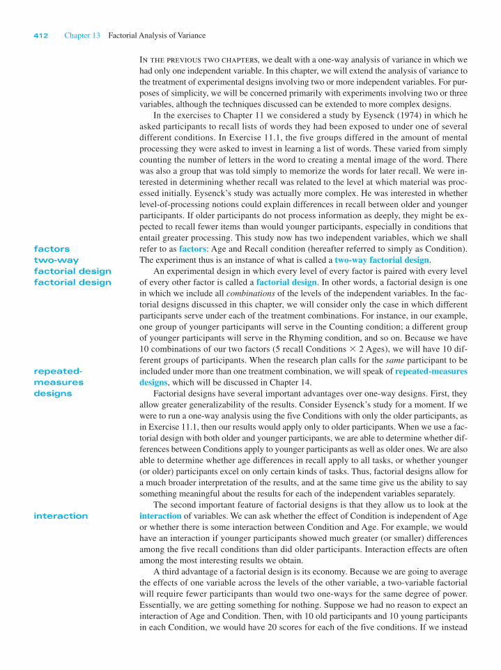
13.1 An Extension of the Eysenck Study
As mentioned earlier, Eysenck actually conducted a study varying Age as well as Recall Con-
dition. The study included 50 participants in the 18-to-30-year age range, as well as 50 par-
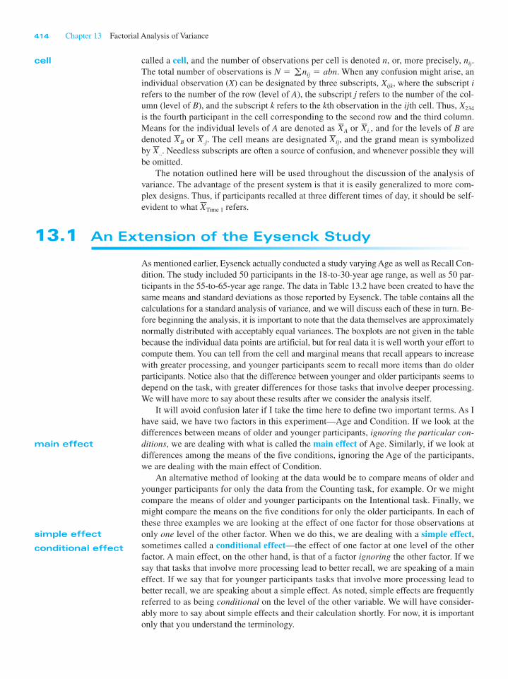
ticipants in the 55-to-65-year age range. The data in Table 13.2 have been created to have the
same means and standard deviations as those reported by Eysenck. The table contains all the
calculations for a standard analysis of variance, and we will discuss each of these in turn. Be-
fore beginning the analysis, it is important to note that the data themselves are approximately
normally distributed with acceptably equal variances. The boxplots are not given in the table
because the individual data points are artificial, but for real data it is well worth your effort to
compute them. You can tell from the cell and marginal means that recall appears to increase
with greater processing, and younger participants seem to recall more items than do older
participants. Notice also that the difference between younger and older participants seems to
depend on the task, with greater differences for those tasks that involve deeper processing.
We will have more to say about these results after we consider the analysis itself.
It will avoid confusion later if I take the time here to define two important terms. As I
have said, we have two factors in this experiment—Age and Condition. If we look at the
differences between means of older and younger participants, ignoring the particular con-ditions, we are dealing with what is called the main effect of Age. Similarly, if we look at
differences among the means of the five conditions, ignoring the Age of the participants,
we are dealing with the main effect of Condition.
An alternative method of looking at the data would be to compare means of older and
younger participants for only the data from the Counting task, for example. Or we might
compare the means of older and younger participants on the Intentional task. Finally, we
might compare the means on the five conditions for only the older participants. In each of
these three examples we are looking at the effect of one factor for those observations at
only one level of the other factor. When we do this, we are dealing with a simple effect, sometimes called a conditional effect—the effect of one factor at one level of the other
factor. A main effect, on the other hand, is that of a factor ignoring the other factor. If we
say that tasks that involve more processing lead to better recall, we are speaking of a main
effect. If we say that for younger participants tasks that involve more processing lead to
better recall, we are speaking about a simple effect. As noted, simple effects are frequently
referred to as being conditional on the level of the other variable. We will have consider-
ably more to say about simple effects and their calculation shortly. For now, it is important
only that you understand the terminology.
cell
main effect
simple effect
conditional effect
Section 13.1 An Extension of the Eysenck Study 415
Table 13.2 Data and computations for example from Eysenck (1974)
(a) Data:
Recall Conditions Meani.
Counting Rhyming Adjective Imagery Intention
Old 9
8
6
8
10
4
6
5
7
7
7
9
6
6
6
11
6
3
8
7
11
13
8
6
14
11
13
13
10
11
12
11
16
11
9
23
12
10
19
11
10
19
14
5
10
11
14
15
11
11
Mean1j 7.0 6.9 11.0 13.4 12.0 10.06
Young 8
6
4
6
7
6
5
7
9
7
10
7
8
10
4
7
10
6
7
7
14
11
18
14
13
22
17
16
12
11
20
16
16
15
18
16
20
22
14
19
21
19
17
15
22
16
22
22
18
21
Mean2j 6.5 7.6 14.8 17.6 19.3 13.16
Mean.j 6.75 7.25 12.9 15.5 15.65 11.61
(b) Calculations:
SStotal 5 a 1X 2 X.. 2 2 5 19 2 11.61 2 2 1 18 2 11.61 2 2 1 c 1 121 2 11.61 2 2 5 2667.79
SSA 5 nca 1Xi. 2 X.. 2 2 5 10 3 5 3 110.06 2 11.61 2 2 1 113.16 2 11.61 2 2 4 5 240.25
SSC 5 naa 1X.j 2 X.. 2 2 5 10 3 2 3 16.75 2 11.61 2 2 1 17.25 2 11.61 2 2 1 c 1 115.65 2 11.61 2 2 4 5 1514.94
SScells 5 na 1Xij 2 X.. 2 2 5 10 3 17.0 2 11.61 2 2 1 16.9 2 11.61 2 2 1 c 1 119.3 2 11.61 2 2 4 5 1945.49
SSAC 5 SScells 2 SSA 2 SSC 5 1945.49 2 240.25 2 1514.94 5 190.30
SSerror 5 SStotal 2 SScells 5 2667.79 2 1945.49 5 722.30
(continues)
© C
engag
e L
earn
ing 2
013
416 Chapter 13 Factorial Analysis of Variance
Calculations
The calculations for the sums of squares appear in Table 13.2b. Many of these calculations
should be familiar, since they resemble the procedures used with a one-way. For example,
SStotal is computed the same way it was in Chapter 11, which is the way it is always com-
puted. We sum all of the squared deviations of the observations from the grand mean.
The sum of squares for the Age factor (SSA) is nothing but the SStreat that we would
obtain if this were a one-way analysis of variance without the Condition factor. In other
words, we simply sum the squared deviations of the Age means from the grand mean and
multiply by nc. We use nc as the multiplier here because each age has n participants at each
of c levels. (There is no need to remember that multiplier as a formula. Just keep in mind
that it is the number of scores upon which the relevant means are based.) The same proce-
dures are followed in the calculation of SSC, except that here we ignore the presence of the
Age variable.
Having obtained SStotal, SSA, and SSC, we come to an unfamiliar term, SScells. This term
represents the variability of the individual cell means and is in fact only a dummy term; it
will not appear in the summary table. It is calculated just like any other sum of squares.
We take the deviations of the cell means from the grand mean, square and sum them, and
multiply by n, the number of observations per mean. Although it might not be readily ap-
parent why we want this term, its usefulness will become clear when we calculate a sum of
squares for the interaction of Age and Condition. (It may be easier to understand the calcu-
lation of SScells if you think of it as what you would have if you viewed this as a study with
10 “groups” and calculated SSgroups.)
The SScells is a measure of how much the cell means differ. Two cell means may differ
for any of three reasons, other than sampling error: (1) because they come from different
levels of A (Age); (2) because they come from different levels of C (Condition); or (3) be-
cause of an interaction between A and C. We already have a measure of how much the cells
differ, since we know SScells. SSA tells us how much of this difference can be attributed to
differences in Age, and SSC tells us how much can be attributed to differences in Condition.
Whatever cannot be attributed to Age or Condition must be attributable to the interaction
between Age and Condition (SSAC). Thus SScells has been partitioned into its three constitu-
ent parts—SSA, SSC, and SSAC. To obtain SSAC, we simply subtract SSA and SSC from SScells.
Whatever is left over is SSAC. In our example,
SSAC 5 SScells 2 SSA 2 SSC
5 1945.49 2 240.25 2 1514.94 5 190.30
All that we have left to calculate is the sum of squares due to error. Just as in the one-
way analysis, we will obtain this by subtraction. The total variation is represented by SStotal.
SScells
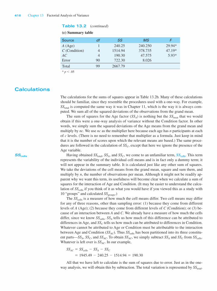
(c) Summary table
Source df SS MS F
A (Age)
C (Condition)
ACError
1
4
4
90
240.25
1514.94
190.30
722.30
240.250
378.735
47.575
8.026
29.94*
47.19*
5.93*
Total 99 2667.79
* p , .05
Table 13.2 (continued)
Section 13.1 An Extension of the Eysenck Study 417
Of this total, we know how much can be attributed to A, C, and AC. What is left over
represents unaccountable variation or error. Thus
SSerror 5 SStotal 2 1SSA 1 SSC 1 SSAC 2However, since SSA 1 SSC 1 SSAC 5 SScells, it is simpler to write
SSerror 5 SStotal 2 SScells
This provides us with our sum of squares for error, and we now have all of the necessary
sums of squares for our analysis.
A more direct, but tiresome, way to calculate SSerror exists, and it makes explicit just what
the error sum of squares is measuring. SSerror represents the variation within each cell, and as
such can be calculated by obtaining the sum of squares for each cell separately. For example,
SScell11 5 (9 2 7)2 1 (8 2 7)2 1 c 1 (7 2 7)2 5 30
We could perform a similar operation on each of the remaining cells, obtaining
SScell115 30.0
SScell125 40.9
c c
SScell25
SSerror
564.1
722.30
The sum of squares within each cell is then summed over the 10 cells to produce SSerror.
Although this is the hard way of computing an error term, it demonstrates that SSerror is in
fact the sum of within-cell variation. When we come to mean squares, MSerror will turn out
to be just the average of the variances within each of the 2 3 5 = 10 cells.
Table 13.2c shows the summary table for the analysis of variance. The source col-
umn and the sum of squares column are fairly obvious from what you already know. Next
look at the degrees of freedom. The calculation of df is straightforward. The total number
of degrees of freedom (dftotal) is always equal to N – 1. The degrees of freedom for Age
and Condition are the number of levels of the variable minus 1. Thus, dfA 5 a 2 1 5 1
and dfC 5 c 2 1 5 4. The number of degrees of freedom for any interaction is sim-
ply the product of the degrees of freedom for the components of that interaction. Thus,
dfAC 5 dfA 3 dfC 5 1a 2 1 2 1c 2 1 2 5 1 3 4 5 4. These three rules apply to any analy-
sis of variance, no matter how complex. The degrees of freedom for error can be obtained
either by subtraction (dferror 5 dftotal 2 dfA 2 dfC 2 dfAC), or by realizing that the error
term represents variability within each cell. Because each cell has n –1 df, and since there
are ac cells, dferror 5 ac 1n 2 1 2 5 2 3 5 3 9 5 90.
Just as with the one-way analysis of variance, the mean squares are again obtained by
dividing the sums of squares by the corresponding degrees of freedom. This same proce-
dure is used in any analysis of variance.
Finally, to calculate F, we divide each MS by MSerror. Thus for Age, FA 5 MSA/MSerror;
for Condition, FC 5 MSC/MSerror; and for AC, FAC 5 MSAC/MSerror. To appreciate why
MSerror is the appropriate divisor in each case, we will digress briefly in a moment and con-
sider the underlying structural model and the expected mean squares. First, however, we
need to consider what the results of this analysis tell us.
Interpretation
From the summary table in Table 13.2c, you can see that there were significant effects
for Age, Condition, and their interaction. In conjunction with the means, it is clear that
younger participants recall more items overall than do older participants. It is also clear
418 Chapter 13 Factorial Analysis of Variance
that those tasks that involve greater depth of processing lead to better recall overall than do
tasks involving less processing. This is in line with the differences we found in Chapter 11.
The significant interaction tells us that the effect of one variable depends on the level of
the other variable. For example, differences between older and younger participants on the
easier tasks such as counting and rhyming are much less than age differences on tasks, such
as imagery and intentional, that involve greater depths of processing. Another view is that
differences among the five conditions are less extreme for the older participants than they
are for the younger ones.
These results support Eysenck’s hypothesis that older participants do not perform as well
as younger participants on tasks that involve a greater depth of processing of information,
but perform about equally with younger participants when the task does not involve much
processing. These results do not mean that older participants are not capable of processing
information as deeply. Older participants simply may not make the effort that younger par-
ticipants do. Whatever the reason, however, they do not perform as well on those tasks.
13.2 Structural Models and Expected Mean Squares
Recall that in discussing a one-way analysis of variance, we employed the structural model
Xij 5 m 1 tj 1 eij
where tj 5 mj 2 m represented the effect of the jth treatment. In a two-way design we have
two “treatment” variables (call them A and B) and their interaction. These can be repre-
sented in the model by a, b, and ab, producing a slightly more complex model. This model
can be written as
Xijk 5 m 1 ai 1 bj 1 abij 1 eijk
where
Xijk 5 any observation
m 5 the grand mean
ai 5 the effect of Factor Ai 5 mAi2 m
bj 5 the effect of Factor Bj 5 mBj2 m
abij 5 the interaction effect of Factor Ai and Factor Bj
5 m 2 mAi2 mBj
1 mij;ai
abij 5 aj
abij 5 0
eijk 5 the unit of error associated with observation Xijk
5 N 10,s2e 2
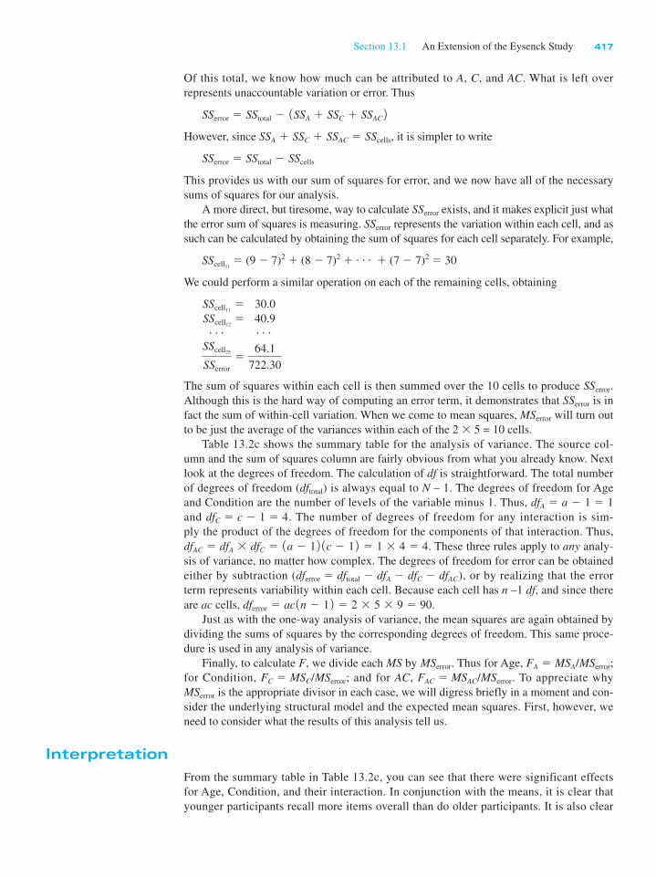
From this model it can be shown that with fixed variables the expected mean squares are
those given in Table 13.3. It is apparent that the error term is the proper denominator for
each F ratio, because the E(MS) for any effect contains only one term other than s2e.
Table 13.3 Expected mean squares for two-way analysis of variance (fixed)
Source E(MS)
ABABError
s2e 1 nbu2
a
s2e 1 nau2
b
s2e 1 nu2
ab
s2e
where u2a 5
Sa2j
a 2 15
S 1mi 2 m 2 2a 2 1
© Cengage Learning 2013
Section 13.3 Interactions 419
If H0 is true, then mA15 mA2
5 m and u2a, and thus nbu2
a, will be 0. In this case, F will be
the ratio of two different estimates of error, and its expectation is approximately 1 and will
be distributed as the standard (central) F distribution. If H0 is false, however, u2a will not be
0 and F will have an expectation greater than 1 and will not follow the central F distribu-
tion. The same logic applies to tests on the effects of B and AB. We will return to structural
models and expected mean squares in Section 13.8 when we discuss alternative designs
that we might use. There we will see that the expected mean squares can become much
more complicated, but the decision on the error term for a particular effect will reflect the
logic of what we have seen here.
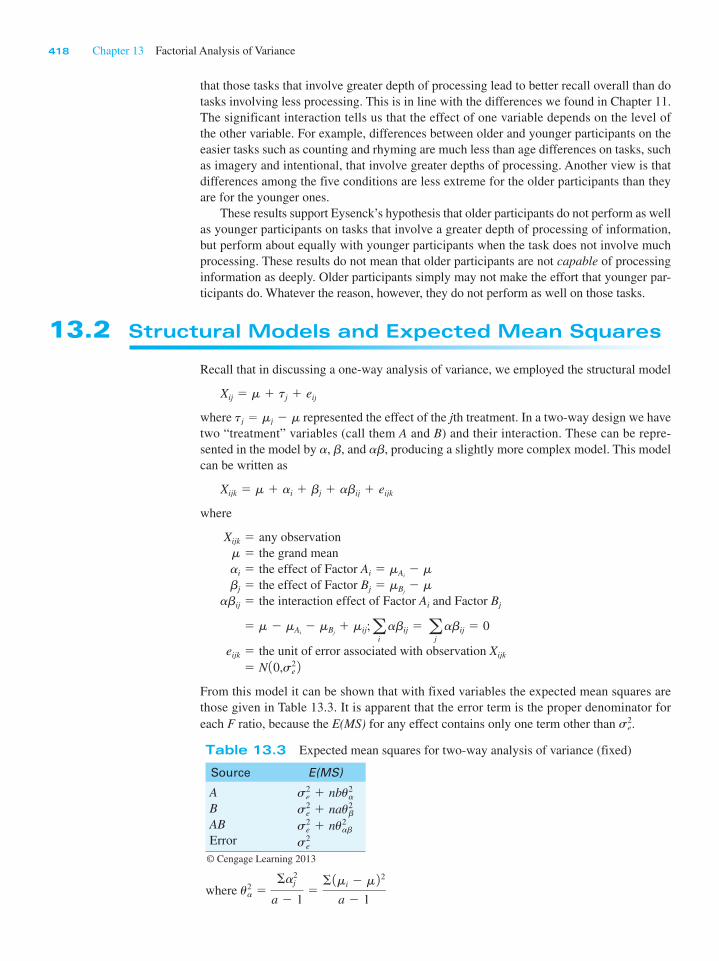
13.3 Interactions
One of the major benefits of factorial designs is that they allow us to examine the interac-
tion of variables. Indeed, in many cases, the interaction term may well be of greater interest
than are the main effects (the effects of factors taken individually). Consider, for example,
the study by Eysenck. The means are plotted in Figure 13.1 for each age group separately.
Here you can see clearly what I referred to in the interpretation of the results when I said
that the differences due to Conditions were greater for younger participants than for older
ones. The fact that the two lines are not parallel is what we mean when we speak of an
interaction. If Condition differences were the same for the two Age groups, then the lines
would be parallel—whatever differences between Conditions existed for younger partici-
pants would be equally present for older participants. This would be true regardless of
whether younger participants were generally superior to older participants or whether the
two groups were comparable. Raising or lowering the entire line for younger participants
Consider for a moment the test of the effect of Factor A:
E 1MSA 2E 1MSerror 2 5
s2e 1 nbu2
a
s2e
1
7.5
10
12.5
Est
imat
ed M
argi
nal M
eans
Estimated Marginal Means of Recall
15
17.5
20
2 3Condition
4 5
AgeYoung Older
Figure 13.1 Cell means for data in Table 13.2
© C
engag
e L
earn
ing 2
013

420 Chapter 13 Factorial Analysis of Variance
would change the main effect of Age, but it would have no effect on the interaction because
it would not affect the degree of parallelism between the lines.
It may make the situation clearer if you consider several plots of cell means that repre-
sent the presence or absence of an interaction. In Figure 13.2 the first three plots represent
the case in which there is no interaction. In all three cases the lines are parallel, even when
they are not straight. Another way of looking at this is to say that the simple effect of Factor B
at A1 is the same as it is at A2 and at A3. In the second set of three plots, the lines clearly are
not parallel. In the first, one line is flat and the other rises. In the second, the lines actually
cross. In the third, the lines do not cross, but they move in opposite directions. In every
case, the simple effect of B is not the same at the different levels of A. Whenever the lines
are (significantly) nonparallel, we say that we have an interaction.
Many people will argue that if you find a significant interaction, the main effects should be
ignored. I have come to accept this view, in part because of comments on the Web by Gary
McClelland. (McClelland, 2008, downloaded on 2/3/2011 from http://finzi.psych.upenn
.edu/Rhelp10/2008-February/153837.html.) He argues that with a balanced design (equal
cell frequencies), what we call the main effect of A is actually the average of the simple ef-
fects of A. But if we have a significant interaction that is telling us that the simple effects are
different from each other, and an average of them has little or no meaning. Moreover, when
I see an interaction my first thought is to look specifically at simple effects of one variable at
specific levels of the other, which is far more informative than worrying about main effects.
This discussion of the interaction effects has focused on examining cell means. I have
taken that approach because it is the easiest to see and has the most to say about the results
of the experiment. Rosnow and Rosenthal (1989) have pointed out that a more accurate
way to look at an interaction is first to remove any row and column effects from the data.
They raise an interesting point, but most interactions are probably better understood in
terms of the explanation above.
13.4 Simple Effects
I earlier defined a simple effect as the effect of one factor (independent variable) at one
level of the other factor—for example, the differences among Conditions for the younger
participants. The analysis of simple effects can be an important technique for analyzing
data that contain significant interactions. In a very real sense, it allows us to “tease apart”
interactions.
I will use the Eysenck data to illustrate how to calculate and interpret simple effects.
Table 13.4 shows the cell means and the summary table reproduced from Table 13.2. The
table also contains the calculations involved in obtaining all the simple effects.
The first summary table in Table 13.4c reveals significant effects due to Age, Condi-
tion, and their interaction. We already discussed these results earlier in conjunction with
the original analysis. As I said there, the presence of an interaction means that there are
Cel
l Mea
nsNo Interaction
A3A2
B1
B2
A1 A3A2
B1B2
A1 A3A2
B1
B2
A1
Cel
l Mea
ns
Interaction
A3A2
B1
B2
A1 A3A2
B1
B2
A1 A3A2
B1
B2
A1
Figure 13.2 Illustration of possible noninteractions and interactions
© C
engag
e L
earn
ing 2
013

Section 13.4 Simple Effects 421
Table 13.4 Illustration of calculation of simple effects (data taken from Table 13.2)
(a) Cell means (n = 10)
Counting Rhyming Adjective Imagery Intention Mean
OlderYounger
7.0
6.5
6.9
7.6
11.0
14.8
13.4
17.6
12.0
19.3
10.06
13.16
Mean 6.75 7.25 12.90 15.50 15.65 11.61
(b) Calculations
Conditions at Each Age
SSC at Old 5 10 3 3 17.0 2 10.06 2 2 1 16.9 2 10.06 2 2 1 c 1 112 2 10.06 2 2 4 5 351.52
SSC at Young 5 10 3 316.5 2 13.162 2 1 17.6 2 13.162 2 1 c 1 119.3 2 13.162 2 4 5 1353.72
Age at Each Condition
SSA at Counting 5 10 3 3 17.0 2 6.75 2 2 1 16.5 2 6.75 2 2 4 5 1.25
SSA at Rhyming 5 10 3 3 16.9 2 7.25 2 2 1 17.6 2 7.25 2 2 4 5 2.45
SSA at Adjective 5 10 3 3 111.0 2 12.9 2 2 1 114.8 2 12.9 2 2 4 5 72.2
SSA at Imagery 5 10 3 3 113.4 2 15.5 2 2 1 117.6 2 15.5 2 2 4 5 88.20
SSA at Intentional 5 10 3 3 112.0 2 15.65 2 2 1 119.3 2 15.65 2 2 4 5 266.45
(c) Summary Tables
Overall Analysis
Source df SS MS F
A (Age)
C (Condition
ACError
1
4
4
90
240.25
1514.94
190.30
722.30
240.25
378.735
47.575
8.026
29.94*
47.19*
5.93*
Total 99 2667.79
* p , .05
Simple Effects
Source df SS MS F
ConditionsC at Old
C at Young
AgeA at Counting
A at Rhyming
A at Adjective
A at Imagery
A at Intentional
Error
4
4
1
1
1
1
1
90
351.52
1353.72
1.25
2.45
72.20
88.20
266.45
722.30
87.88
338.43
1.25
2.45
72.20
88.20
266.45
8.03
10.95*
42.15*
,1
,1
9.00*
10.99*
33.20*
* p , .05 © C
engag
e L
earn
ing 2
013
422 Chapter 13 Factorial Analysis of Variance
different Condition effects for the two Ages, and there are different Age effects for the five
Conditions. It thus becomes important to ask whether our general Condition effect really
applies for older as well as younger participants, and whether there really are Age differ-
ences under all Conditions. The analysis of these simple effects is found in Table 13.4b and
the second half of Table 13.4c. I have shown all possible simple effects for the sake of com-
pleteness of the example, but in general you should calculate only those effects in which
you are interested. When you test many simple effects you either raise the familywise error
rate to unacceptable levels or else you control the familywise error rate at some reasonable
level and lose power for each simple effect test. One rule of thumb is “Don’t calculate a
contrast or simple effect unless it is relevant to your discussion when you write up the re-
sults.” The more effects you test, the higher the familywise error rate will be.
Calculation of Simple Effects
In Table 13.4b you can see that SSC at Old is calculated in the same way as any sum of
squares. We simply calculate SSC using only the data for the older participants. If we con-
sider only those data, the five Condition means are 7.0, 6.9, 11.0, 13.4, and 12.0. Thus, the
sum of squares will be
SSC at Old 5 na 1X1j 2 X1. 2 2 5 10 3 3 17 2 10.06 2 2 1 16.9 2 10.06 2 2 1 c 1 112 2 10.06 2 2 4 5 351.52
The other simple effects are calculated in the same way—by ignoring all data in which you
are not at the moment interested. The sum of squares for the simple effect of Condition for
older participants (351.52) is the same value as you would have obtained in Exercise 11.1
when you ran a one-way analysis of variance on only the data from older participants.
The degrees of freedom for the simple effects are calculated in the same way as for the
corresponding main effects. This makes sense because the number of means we are com-
paring remains the same. Whether we use all of the participants or only some of them, we
are still comparing five conditions and have 5 2 1 5 4 df for Conditions.
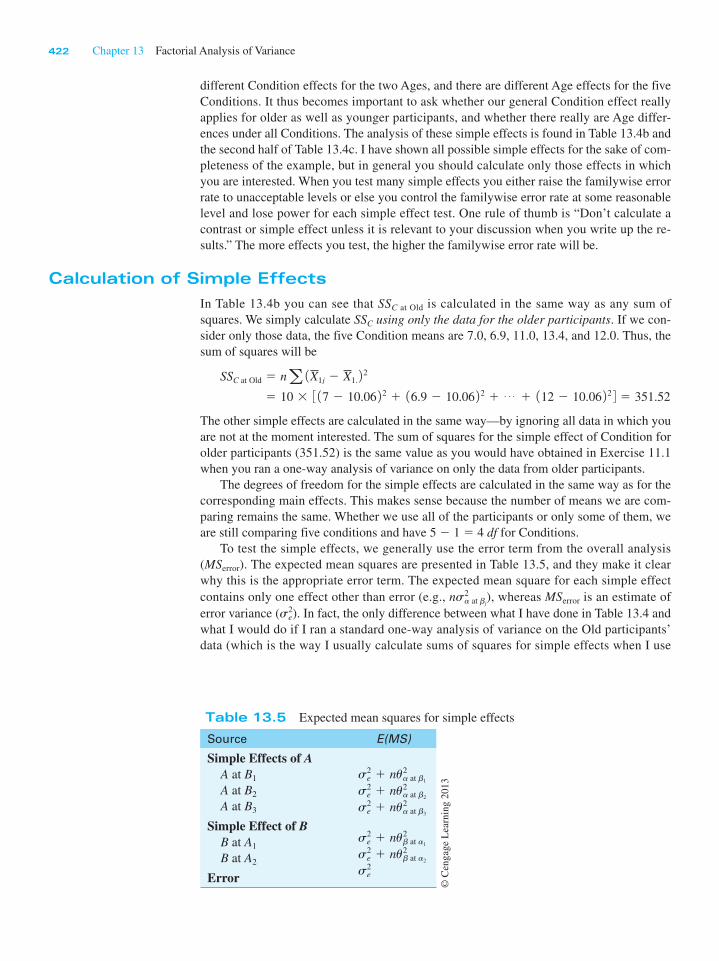
To test the simple effects, we generally use the error term from the overall analysis
(MSerror). The expected mean squares are presented in Table 13.5, and they make it clear
why this is the appropriate error term. The expected mean square for each simple effect
contains only one effect other than error (e.g., ns2a at bj
), whereas MSerror is an estimate of
error variance (s2e). In fact, the only difference between what I have done in Table 13.4 and
what I would do if I ran a standard one-way analysis of variance on the Old participants’
data (which is the way I usually calculate sums of squares for simple effects when I use
Table 13.5 Expected mean squares for simple effects
Source E(MS)
Simple Effects of AA at B1
A at B2
A at B3
Simple Effect of BB at A1
B at A2
Error
s2e 1 nu2
a at b1
s2e 1 nu2
a at b2
s2e 1 nu2
a at b3
s2e 1 nu2
b at a1
s2e 1 nu2
b at a2
s2e
© C
engag
e L
earn
ing 2
013
Section 13.5 Analysis of Variance Applied to the Effects of Smoking 423
computer software) is the error term. MSerror is normally based on all the data because it is
a better estimate with more degrees of freedom.
Interpretation
From the column labeled F in the bottom table in Table 13.4c, it is evident that differences
due to Conditions occur for both ages although the sum of squares for the older participants
is only about one-quarter of what it is for the younger ones. With regard to the Age effects,
however, no differences occur on the lower-level tasks of counting and rhyming, but differ-
ences do occur on the higher-level tasks. In other words, differences between age groups
show up on only those tasks involving higher levels of processing. This is basically what
Eysenck set out to demonstrate.
In general, we seldom look at simple effects unless a significant interaction is present.
However, it is not difficult to imagine data for which an analysis of simple effects would be
warranted even in the face of a nonsignificant interaction, or to imagine studies in which
the simple effects are the prime reason for conducting the experiment.
Additivity of Simple Effects
All sums of squares in the analysis of variance (other than SStotal) represent a partitioning
of some larger sum of squares, and the simple effects are no exception. The simple effect
of Condition at each level of Age represents a partitioning of SSC and SSA 3 C, whereas the
effects of Age at each level of Condition represent a partitioning of SSA and SSA 3 C. Thus
aSSC at A 5 351.52 1 1353.72 5 1705.24
SSC 1 SSA3C 5 1514.94 1 190.30 5 1705.24
and
aSSA at C 5 1.25 1 2.45 1 72.20 1 88.20 1 266.45 5 430.55
SSA 1 SSA3C 5 240.25 1 190.30 5 430.55
A similar additive relationship holds for the degrees of freedom. The fact that the sums of
squares for simple effects sum to the combined sums of squares for the corresponding main
effect and interaction affords us a quick and simple check on our calculations.
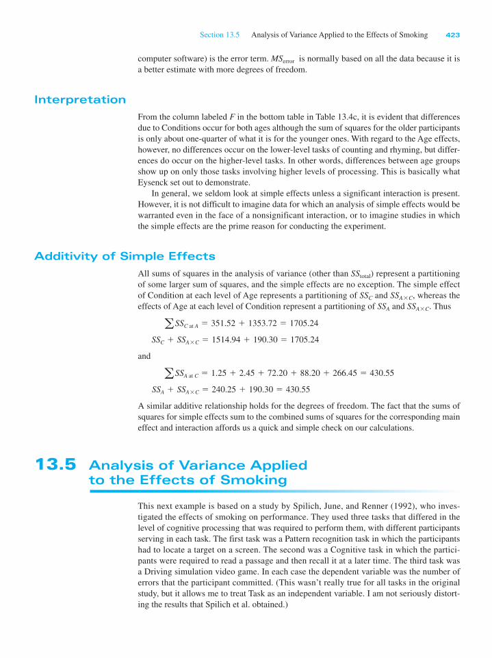
13.5 Analysis of Variance Applied to the Effects of Smoking
This next example is based on a study by Spilich, June, and Renner (1992), who inves-
tigated the effects of smoking on performance. They used three tasks that differed in the
level of cognitive processing that was required to perform them, with different participants
serving in each task. The first task was a Pattern recognition task in which the participants
had to locate a target on a screen. The second was a Cognitive task in which the partici-
pants were required to read a passage and then recall it at a later time. The third task was
a Driving simulation video game. In each case the dependent variable was the number of
errors that the participant committed. (This wasn’t really true for all tasks in the original
study, but it allows me to treat Task as an independent variable. I am not seriously distort-
ing the results that Spilich et al. obtained.)
424 Chapter 13 Factorial Analysis of Variance
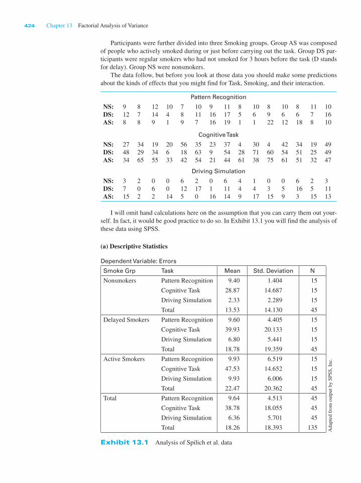
Participants were further divided into three Smoking groups. Group AS was composed
of people who actively smoked during or just before carrying out the task. Group DS par-
ticipants were regular smokers who had not smoked for 3 hours before the task (D stands
for delay). Group NS were nonsmokers.
The data follow, but before you look at those data you should make some predictions
about the kinds of effects that you might find for Task, Smoking, and their interaction.
Pattern Recognition
NS: 9 8 12 10 7 10 9 11 8 10 8 10 8 11 10
DS: 12 7 14 4 8 11 16 17 5 6 9 6 6 7 16
AS: 8 8 9 1 9 7 16 19 1 1 22 12 18 8 10
Cognitive Task
NS: 27 34 19 20 56 35 23 37 4 30 4 42 34 19 49
DS: 48 29 34 6 18 63 9 54 28 71 60 54 51 25 49
AS: 34 65 55 33 42 54 21 44 61 38 75 61 51 32 47
Driving Simulation
NS: 3 2 0 0 6 2 0 6 4 1 0 0 6 2 3
DS: 7 0 6 0 12 17 1 11 4 4 3 5 16 5 11
AS: 15 2 2 14 5 0 16 14 9 17 15 9 3 15 13
I will omit hand calculations here on the assumption that you can carry them out your-
self. In fact, it would be good practice to do so. In Exhibit 13.1 you will find the analysis of
these data using SPSS.
(a) Descriptive Statistics
Dependent Variable: Errors
Smoke Grp Task Mean Std. Deviation N
Nonsmokers Pattern Recognition 9.40 1.404 15
Cognitive Task 28.87 14.687 15
Driving Simulation 2.33 2.289 15
Total 13.53 14.130 45
Delayed Smokers Pattern Recognition 9.60 4.405 15
Cognitive Task 39.93 20.133 15
Driving Simulation 6.80 5.441 15
Total 18.78 19.359 45
Active Smokers Pattern Recognition 9.93 6.519 15
Cognitive Task 47.53 14.652 15
Driving Simulation 9.93 6.006 15
Total 22.47 20.362 45
Total Pattern Recognition 9.64 4.513 45
Cognitive Task 38.78 18.055 45
Driving Simulation 6.36 5.701 45
Total 18.26 18.393 135
Exhibit 13.1 Analysis of Spilich et al. data
Adap
ted f
rom
outp
ut
by S
PS
S, In
c.

Section 13.5 Analysis of Variance Applied to the Effects of Smoking 425
An SPSS summary table for a factorial design differs somewhat from others you have
seen in that it contains additional information. The line labeled “Corrected model” is the
sum of the main effects and the interaction. As such its sum of squares is what we earlier
called SScells. The line labeled “Intercept” is a test on the grand mean, here showing that the
grand mean is significantly different from 0.00, which is hardly a surprise. Near the bottom
the line labeled “Corrected total” is what we normally label “Total,” and the line that they
label “Total” is 1gX2/N 2 . These extra lines rarely add anything of interest.
The summary table reveals that there are significant effects due to Task and to the interac-
tion of Task and SmokeGrp, but there is no significant effect due to the SmokeGrp variable.
(b) Summary table
Tests of Between-Subjects Effects
Dependent Variable: Errors
Source
Type III Sum
of Squares df
Mean
Square F Sig.
Partial
Eta
Squared
Noncent.
Parameter
Observed
Powerb
Corrected Model 31744.726a 8 3968.091 36.798 .000 .700 294.383 1.000
Intercept 45009.074 1 45009.074 417.389 .000 .768 417.389 1.000
Task 28661.526 2 14330.763 132.895 .000 .678 265.791 1.000
SmokeGrp 1813.748 2 906.874 8.410 .000 .118 16.820 .961
Task* SmokeGrp 1269.452 4 317.363 2.943 .023 .085 11.772 .776
Error 13587.200 126 107.835
Total 90341.000 135
Corrected Total 45331.926 134
a R Squared = .700 (Adjusted R Squared = .681)b Computed using alpha = .05
(c) Interaction plot
Exhibit 13.1 (Continued)
50
40
30
Mea
n E
rror
s
20
10
0
Nonsmokers Delayed smokers
SmokeGrp
Marginal Mean Errors
Active smokers
TaskPattern recognitionCognitive taskDriving simulation
426 Chapter 13 Factorial Analysis of Variance
The Task effect is of no interest, because it simply says that people make more errors on some
kinds of tasks than others. This is like saying that your basketball team scored more points in
yesterday’s game than did your soccer team. You can see the effects graphically in the interac-
tion plot, which is self-explanatory. Notice in the table of descriptive statistics that the stand-
ard deviations, and thus the variances, are very much higher on the Cognitive task than on the
other two tasks. We will want to keep this in mind when we carry out further analyses.
13.6 Comparisons Among Means
All of the procedures discussed in Chapter 12 are applicable to the analysis of factorial de-
signs. Thus we can test the differences among the five Condition means in the Eysenck ex-
ample, or the three SmokeGrp means in the Spilich example using standard linear contrasts,
the Bonferroni t test, the Tukey test, or any other procedure. Keep in mind, however, that we
must interpret the “n” that appears in the formulae in Chapter 12 to be the number of obser-
vations on which each treatment mean was based. Because the Condition means are based on
(a 3 n) observations that is the value that you would enter into the formula, not n. Because
the interaction of Task with SmokeGrp is significant, I would be unlikely to want to examine
the main effects further. However, an examination of simple effects will be very useful.
In the Spilich smoking example, there is no significant effect due to SmokeGrp, so you
would probably not wish to run contrasts among the three levels of that variable. Because
the dependent variable (errors) is not directly comparable across tasks, it makes no sense to
look for specific Task group differences there. We could do so, but no one would be likely
to care. (Remember the basketball and soccer teams referred to above.) However, I would
expect that smoking might have its major impact on cognitive tasks, and you might wish
to run either a single contrast (active smokers versus nonsmokers) or multiple comparisons
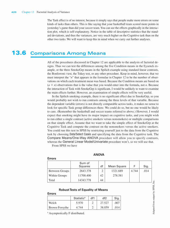
on that simple effect. Assume that we want to take the simple effect of SmokeGrp at the
Cognitive Task and compute the contrast on the nonsmokers versus the active smokers.
You could run this test in SPSS by restricting yourself just to the data from the Cognitive
task by choosing Data/Select Cases and specifying the data from the Cognitive task. The
Compare Means/One-Way ANOVA procedure will allow you to specify contrasts,
whereas the General Linear Model/Univariate procedure won’t, so we will use that.
From SPSS we have
ANOVAErrors
Sum of Squares df Mean Square F Sig.
Between Groups 2643.378 2 1321.689 4.744 .014
Within Groups 11700.400 42 278.581
Total 14343.778 44
Robust Tests of Equality of MeansErrors
Statistica df1 df2 Sig.
Welch 5.970 2 27.527 .007
Brown-Forsythe 4.744 2 38.059 .014
a Asymptotically F distributed. Adap
ted f
rom
outp
ut
by S
PS
S, In
c.
Section 13.7 Power Analysis for Factorial Experiments 427
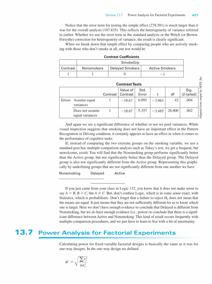
Notice that the error term for testing the simple effect (278.581) is much larger than it
was for the overall analysis (107.835). This reflects the heterogeneity of variance referred
to earlier. Whether we use the error term in the standard analysis or the Welch (or Brown-
Forsythe) correction for heterogeneity of variance, the result is clearly significant.
When we break down that simple effect by comparing people who are actively smok-
ing with those who don’t smoke at all, our test would be
Contrast Coefficients
SmokeGrp
Contrast Nonsmokers Delayed Smokers Active Smokers
1 1 0 21
Contrast Tests
Contrast
Value of
Contrast
Std.
Error t df
Sig.
(2-tailed)
Errors Assume equal
variances
1 218.67 6.095 23.063 42 .004
Does not assume
equal variances
1 218.67 5.357 23.485 28.000 .002
And again we see a significant difference of whether or not we pool variances. While
visual inspection suggests that smoking does not have an important effect in the Pattern
Recognition or Driving condition, it certainly appears to have an effect in when it comes to
the performance of cognitive tasks.
If, instead of comparing the two extreme groups on the smoking variable, we use a
standard post hoc multiple comparison analysis such as Tukey’s test, we get a frequent, but
unwelcome, result. You will find that the Nonsmoking group performs significantly better
than the Active group, but not significantly better than the Delayed group. The Delayed
group is also not significantly different from the Active group. Representing this graphi-
cally by underlining groups that are not significantly different from one another we have
Nonsmoking Delayed Active
If you just came from your class in Logic 132, you know that it does not make sense to
say A 5 B, B 5 C, but A ? C. But, don’t confuse Logic, which is in some sense exact, with
Statistics, which is probabilistic. Don’t forget that a failure to reject H0 does not mean that
the means are equal. It just means that they are not sufficiently different for us to know which
one is larger. Here we don’t have enough evidence to conclude that Delayed is different from
Nonsmoking, but we do have enough evidence (i.e., power) to conclude that there is a signif-
icant difference between Active and Nonsmoking. This kind of result occurs frequently with
multiple-comparison procedures, and we just have to learn to live with a bit of uncertainty.
13.7 Power Analysis for Factorial Experiments
Calculating power for fixed-variable factorial designs is basically the same as it was for
one-way designs. In the one-way design we defined
f r 5 Åat2j
ks2e
Adap
ted f
rom
outp
ut
by S
PS
S, In
c.

428 Chapter 13 Factorial Analysis of Variance
and
f 5 f r"n
wheregt2j 5 g 1mj 2 m 2 2, k 5 the number of treatments, and n = the number of observa-
tions in each treatment. And, as with the one-way, f r is often denoted as f, which is the way
G*Power names it. In the two-way and higher-order designs we have more than one “treat-
ment,” but this does not alter the procedure in any important way. If we let ai 5 mi. 2 m,
and bj 5 m.j 2 m, where mi. represents the parametric mean of Treatment Ai (across all
levels of B) and m.j represents the parametric mean of Treatment Bj (across all levels of A),
then we can define the following terms:
f ra 5 Åaa2j
as2e
fa 5 f ra"nb
and
f rb 5 Åab2j
bs2e
fb 5 f rb"na
Examination of these formulae reveals that to calculate the power against a null hypothesis
concerning A, we act as if variable B did not exist. To calculate the power of the test against
a null hypothesis concerning B, we similarly act as if variable A did not exist.
Calculating the power against the null hypothesis concerning the interaction follows
the same logic. We define
f rab 5 Åaab2ij
abs2e
fab 5 f rab"n
where abij is defined as for the underlying structural model 1abij 5 m 2 mi. 2 m.j 1 mij 2 . Given fab, we can simply obtain the power of the test just as we did for the one-way design.
To illustrate the calculation of power for an interaction, we will use the cell and mar-
ginal means for the Spilich et al. study. These means are
Pattern Cognitive Driving MeanNonsmoker 9.400 28.867 2.333 13.533
Delayed 9.600 39.933 6.800 18.778
Active 9.933 47.533 9.933 22.467
Mean 9.644 38.778 6.356 18.259
f r 5 ÅSab2ij
abs2e
5 Å 19.40 2 13.533 2 9.644 1 18.2592 2 1 c1 19.933 2 22.467 2 6.356 1 18.2592 23 3 3 3 107.835
5 Å20.088 1 c 1 0.398
970.5155 Å 84.626
970.5155 "0.087 5 .295
© C
engag
e L
earn
ing
2013

Section 13.7 Power Analysis for Factorial Experiments 429
Assume that we want to calculate the expected level of power in an exact replication of
Spilich’s experiment assuming that Spilich has exactly estimated the corresponding popu-
lation parameters. (He almost certainly has not, but those estimates are the best guess we
have of the parameters.) Using 0.295 as the effect size (which G*Power calls f) we have the
following result.
Therefore, if the means and variances that Spilich obtained accurately reflect the cor-
responding population parameters, the probability of obtaining a significant interaction in a
replication of that study is .776, which agrees exactly with the results obtained by SPSS.
To remind you what the graph at the top is all about, the solid distribution represents
the distribution of F under the null hypothesis. The dashed distribution represents the (non-
central) distribution of F given the population means we expect. The vertical line shows the
critical value of F under the null hypothesis. The shaded area labeled b represents those val-
ues of F that we will obtain, if estimated parameters are correct, that are less than the criti-
cal value of F and will not lead to rejection of the null hypothesis. Power is then 1 2 b.
In certain situations a two-way factorial is more powerful than are two separate one-
way designs, in addition to the other advantages that accrue to factorial designs. Consider
two hypothetical studies, where the number of participants per treatment is held constant
across both designs.
In Experiment 1 an investigator wishes to examine the efficacy of four different treat-
ments for post-traumatic stress disorder (PTSD) in rape victims. She has chosen to use both
male and female therapists. Our experimenter is faced with two choices. She can run a one-
way analysis on the four treatments, ignoring the sex of the therapist (SexTher) variable
Wit
h k
ind p
erm
issi
on f
rom
F
ranz
Fau
l, E
dgar
Erd
feld
er, A
lber
t-G
eorg
Lan
g a
nd A
xel
Buch
ner
/G*P
ow
er

430 Chapter 13 Factorial Analysis of Variance
entirely, or she can run a 4 3 2 factorial analysis on the four treatments and two sexes. In
this case the two-way has more power than the one-way. In the one-way design we would
ignore any differences due to SexTher and the interaction of Treatment with SexTher, and
these would go toward increasing the error term. In the two-way we would take into ac-
count differences that can be attributed to SexTher and to the interaction between Treat-
ment and SexTher, thus removing them from the error term. The error term for the two-way
would thus be smaller than for the one-way, giving us greater power.
For Experiment 2, consider the experimenter who had originally planned to use only
female therapists in her experiment. Her error term would not be inflated by differences
among SexTher and by the interaction, because neither of those exist. If she now expanded
her study to include male therapists, SStotal would increase to account for additional effects
due to the new independent variable, but the error term would remain constant because the
extra variation would be accounted for by the extra terms. Because the error term would
remain constant, she would have no increase in power in this situation over the power she
would have had in her original study, except for an increase in n.
As a general rule, a factorial design is more powerful than a one-way design only when
the extra factors can be thought of as refining or purifying the error term. In other words,
when extra factors or variables account for variance that would normally be incorporated
into the error term, the factorial design is more powerful. Otherwise, all other things being
equal, it is not, although it still possesses the advantage of allowing you to examine the
interactions and simple effects.
You need to be careful about one thing, however. When you add a factor that is a ran-
dom factor (e.g., Classroom) you may actually decrease the power of your test. As you will
see in a moment, in models with random factors the fixed factor, which may well be the
one in which you are most interested, will probably have to be tested using MSinteraction as
the error term instead of MSerror. This is likely to cost you a considerable amount of power.
And you can’t just pretend that the Classroom factor didn’t exist, because then you will
run into problems with the independence of errors. For a discussion of this issue, see Judd,
McClelland, and Culhane (1995).
There is one additional consideration in terms of power that we need to discuss. McClel-
land and Judd (1993) have shown that power can be increased substantially using what they
call “optimal” designs. These are designs in which sample sizes are apportioned to the cells
unequally to maximize power. McClelland has argued that we often use more levels of the
independent variables than we need, and we frequently assign equal numbers of participants
to each cell when in fact we would be better off with fewer (or no) participants in some cells
(especially the central levels of ordinal independent variables). For example, imagine two
independent variables that can take up to five levels, denoted as A1, A2, A3, A4, and A5 for
Factor A, and B1, B2, B3, B4, and B5 for Factor B. McClelland and Judd (1993) show that a
5 3 5 design using all five levels of each variable is only 25% as efficient as a design using
only A1 and A5, and B1 and B5. A 3 3 3 design using A1, A3, and A5, and B1, B3, and B5 is
44% as efficient. I recommend a close reading of their paper.
13.8 Alternative Experimental Designs
For traditional experimental research in psychology, fixed models with crossed independ-
ent variables have long been the dominant approach and will most likely continue to be.
In such designs the experimenter chooses a few fixed levels of each independent variable,
which are the levels that are of primary interest and would be the same levels he or she
would expect to use in a replication. In a factorial design each level of each independent
variable is paired (crossed) with each level of all other independent variables.crossed
Section 13.8 Alternative Experimental Designs 431
However, there are many situations in psychology and education where this traditional
design is not appropriate, just as there are a few cases in traditional experimental work. In
many situations the levels of one or more independent variables are sampled at random
(e.g., we might sample 10 classrooms in a given school and treat Classroom as a factor),
giving us a random factor. In other situations one independent variable is nested within
another independent variable. An example of the latter is when we sample 10 classrooms
from school district A and another 10 classrooms from school district B. In this situation
the district A classrooms will not be found in district B and vice versa, and we call this a
nested design. Random factors and nested designs often go together, which is why they are
discussed together here, though they do not have to.
When we have random and/or nested designs, the usual analyses of variance that we
have been discussing are not appropriate without some modification. The primary problem
is that the error terms that we usually think of are not correct for one or more of the Fs that
we want to compute. In this section I will work through three possible designs, starting
with the traditional fixed model with crossed factors and ending with a random model with
nested factors. I certainly cannot cover all aspects of all possible designs, but the gener-
alization from what I discuss to other designs should be reasonably apparent. I am doing
this for two different reasons. In the first place, modified traditional analyses of variance,
as described below, are quite appropriate in many of these situations. In addition, there has
been a general trend toward incorporating what are called hierarchical models or mixed models in our analyses, and an understanding of those models hinges crucially on the con-
cepts discussed here.
In each of the following sections I will work with the same set of data but with dif-
ferent assumptions about how those data were collected, and with different names for the
independent variables. The raw data that I will use for all examples are the same data that
we saw in Table 13.2 on Eysenck’s study of age and recall under conditions of varying
levels of processing of the material. I will change, however, the variable names to fit with
my example.
One important thing to keep firmly in mind is that virtually all statistical tests operate
within the idea of the results of an infinite number of replications of the experiment. Thus
the Fs that we have for the two main effects and the interaction address the question of “If
the null hypothesis was true and we replicated this experiment 10,000 times, how often
would we obtain an F statistic as extreme as the one we obtained in this specific study?”
If that probability is small, we reject the null hypothesis. There is nothing new there. But
we need to think for a moment about what would produce different F values in our 10,000
replications of the same basic study. Given the design that Eysenck used, every time we
repeated the study we would use one group of older subjects and one group of younger
subjects. There is no variability in that independent variable. Similarly, every time we re-
peat the study we will have the same five Recall Conditions (Counting, Rhyming, Adjec-
tive, Imagery, Intention). So again there is no variability in that independent variable. This
is why we refer to this experiment as a fixed effect design—the levels of the independent
variable are fixed and will be the same from one replication to another. The only reason
why we would obtain different F values from one replication to another is sampling error,
which comes from the fact that each replication uses different subjects. (You will shortly
see that this conclusion does not apply with random factors.)
To review the basic structural model behind the fixed-model analyses that we have been
running up to now, recall that the model was
Xijk 5 m 1 ai 1 bj 1 abij 1 eijk
Over replications the only variability comes from the last term (eijk), which explains why
MSerror can be used as the denominator for all three F tests. That will be important as we go on.
random factor
nested design
random
nested designs
hierarchical
models
mixed models
432 Chapter 13 Factorial Analysis of Variance
A Crossed Experimental Design with Fixed Variables
The original example is what we will class as a crossed experimental design with fixed
factors. In a crossed design each level of one independent variable (factor) is paired with
each level of any other independent variable. For example, both older and younger partici-
pants are tested under each of the five recall conditions. In addition, the levels of the factors
are fixed because these are the levels that we actually want to study—they are not, for ex-
ample, a random sample of ages or of possible methods of processing information.
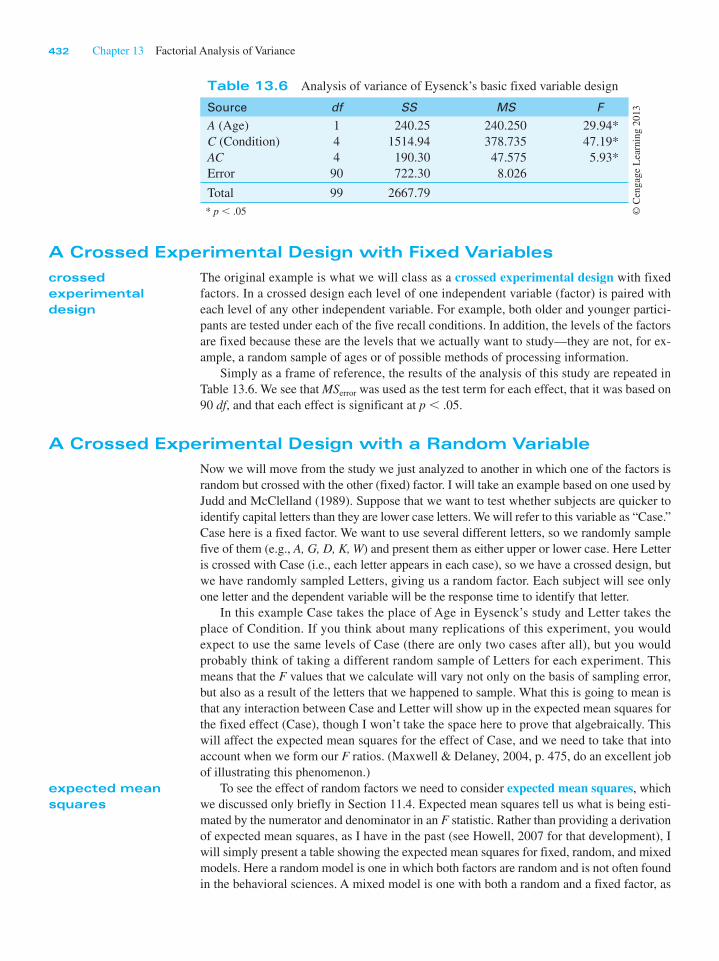
Simply as a frame of reference, the results of the analysis of this study are repeated in
Table 13.6. We see that MSerror was used as the test term for each effect, that it was based on
90 df, and that each effect is significant at p , .05.
A Crossed Experimental Design with a Random Variable
Now we will move from the study we just analyzed to another in which one of the factors is
random but crossed with the other (fixed) factor. I will take an example based on one used by
Judd and McClelland (1989). Suppose that we want to test whether subjects are quicker to
identify capital letters than they are lower case letters. We will refer to this variable as “Case.”
Case here is a fixed factor. We want to use several different letters, so we randomly sample
five of them (e.g., A, G, D, K, W) and present them as either upper or lower case. Here Letter
is crossed with Case (i.e., each letter appears in each case), so we have a crossed design, but
we have randomly sampled Letters, giving us a random factor. Each subject will see only
one letter and the dependent variable will be the response time to identify that letter.
In this example Case takes the place of Age in Eysenck’s study and Letter takes the
place of Condition. If you think about many replications of this experiment, you would
expect to use the same levels of Case (there are only two cases after all), but you would
probably think of taking a different random sample of Letters for each experiment. This
means that the F values that we calculate will vary not only on the basis of sampling error,
but also as a result of the letters that we happened to sample. What this is going to mean is
that any interaction between Case and Letter will show up in the expected mean squares for
the fixed effect (Case), though I won’t take the space here to prove that algebraically. This
will affect the expected mean squares for the effect of Case, and we need to take that into
account when we form our F ratios. (Maxwell & Delaney, 2004, p. 475, do an excellent job
of illustrating this phenomenon.)
To see the effect of random factors we need to consider expected mean squares, which
we discussed only briefly in Section 11.4. Expected mean squares tell us what is being esti-
mated by the numerator and denominator in an F statistic. Rather than providing a derivation
of expected mean squares, as I have in the past (see Howell, 2007 for that development), I
will simply present a table showing the expected mean squares for fixed, random, and mixed
models. Here a random model is one in which both factors are random and is not often found
in the behavioral sciences. A mixed model is one with both a random and a fixed factor, as
crossed
experimental
design
expected mean
squares
Table 13.6 Analysis of variance of Eysenck’s basic fixed variable design
Source df SS MS F
A (Age)
C (Condition)
ACError
1
4
4
90
240.25
1514.94
190.30
722.30
240.250
378.735
47.575
8.026
29.94*
47.19*
5.93*
Total 99 2667.79
* p , .05 © C
engag
e L
earn
ing 2
013
Section 13.8 Alternative Experimental Designs 433
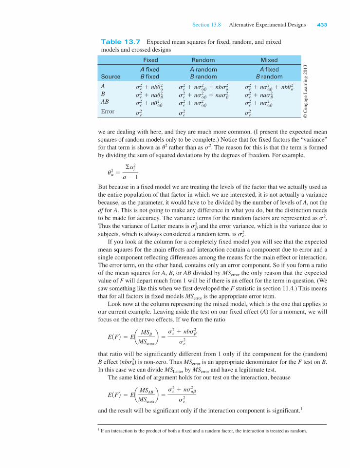
we are dealing with here, and they are much more common. (I present the expected mean
squares of random models only to be complete.) Notice that for fixed factors the “variance”
for that term is shown as u2 rather than as s2. The reason for this is that the term is formed
by dividing the sum of squared deviations by the degrees of freedom. For example,
u2a 5
Sa2j
a 2 1
But because in a fixed model we are treating the levels of the factor that we actually used as
the entire population of that factor in which we are interested, it is not actually a variance
because, as the parameter, it would have to be divided by the number of levels of A, not the
df for A. This is not going to make any difference in what you do, but the distinction needs
to be made for accuracy. The variance terms for the random factors are represented as s2.
Thus the variance of Letter means is s2b and the error variance, which is the variance due to
subjects, which is always considered a random term, is s2e.
If you look at the column for a completely fixed model you will see that the expected
mean squares for the main effects and interaction contain a component due to error and a
single component reflecting differences among the means for the main effect or interaction.
The error term, on the other hand, contains only an error component. So if you form a ratio
of the mean squares for A, B, or AB divided by MS error the only reason that the expected
value of F will depart much from 1 will be if there is an effect for the term in question. (We
saw something like this when we first developed the F statistic in section 11.4.) This means
that for all factors in fixed models MSerror is the appropriate error term.
Look now at the column representing the mixed model, which is the one that applies to
our current example. Leaving aside the test on our fixed effect (A) for a moment, we will
focus on the other two effects. If we form the ratio
E 1F 2 5 Ea MSB
MSerror
b 5s2
e 1 nbs2b
s2e
that ratio will be significantly different from 1 only if the component for the (random)
B effect (nbs2b) is non-zero. Thus MSerror is an appropriate denominator for the F test on B.
In this case we can divide MSLetter by MSerror and have a legitimate test.
The same kind of argument holds for our test on the interaction, because
E 1F 2 5 Ea MSAB
MSerror
b 5s2
e 1 ns2ab
s2e
and the result will be significant only if the interaction component is significant.1
Table 13.7 Expected mean squares for fixed, random, and mixed
models and crossed designs
Fixed Random Mixed
Source
A fixed
B fixed
A random
B random
A fixed
B random
ABAB
Error
s2e 1 nbu2
a
s2e 1 nau2
b
s2e 1 nu2
ab
s2e
s2e 1 ns2
ab 1 nbs2a
s2e 1 ns2
ab 1 nas2b
s2e 1 ns2
ab
s2e
s2e 1 ns2
ab 1 nbu2a
s2e 1 nas2
b
s2e 1 ns2
ab
s2e
1 If an interaction is the product of both a fixed and a random factor, the interaction is treated as random.
© C
engag
e L
earn
ing 2
013
434 Chapter 13 Factorial Analysis of Variance
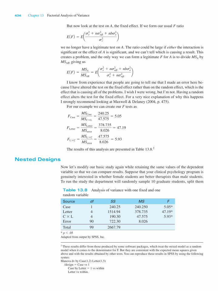
But now look at the test on A, the fixed effect. If we form our usual F ratio
E 1F 2 5 Eas2e 1 ns2
ab 1 nbs2a
s2e
bwe no longer have a legitimate test on A. The ratio could be large if either the interaction is
significant or the effect of A is significant, and we can’t tell which is causing a result. This
creates a problem, and the only way we can form a legitimate F for A is to divide MSA by
MSAB, giving us
E 1F 2 5MSA
MSAB
5 Eas2e 1 ns2
ab 1 nbs2a
s2e 1 ns2
ab
bI know from experience that people are going to tell me that I made an error here be-
cause I have altered the test on the fixed effect rather than on the random effect, which is the
effect that is causing all of the problems. I wish I were wrong, but I’m not. Having a random
effect alters the test for the fixed effect. For a very nice explanation of why this happens
I strongly recommend looking at Maxwell & Delaney (2004, p. 475).
For our example we can create our F tests as
FCase 5MSCase
MSC3L
5240.25
47.5755 5.05
FLetter 5MSLetter
MSerror
5378.735
8.0265 47.19
FL3C 5MSL3C
MSerror
547.575
8.0265 5.93
The results of this analysis are presented in Table 13.8.2
Nested Designs
Now let’s modify our basic study again while retaining the same values of the dependent
variable so that we can compare results. Suppose that your clinical psychology program is
genuinely interested in whether female students are better therapists than male students.
To run the study the department will randomly sample 10 graduate students, split them
Table 13.8 Analysis of variance with one fixed and one
random variable
Source df SS MS F
Case
Letter
C 3 LError
1
4
4
90
240.25
1514.94
190.30
722.30
240.250
378.735
47.575
8.026
5.05*
47.19*
5.93*
Total 99 2667.79
* p , .05
2 These results differ from those produced by some software packages, which treat the mixed model as a random
model when it comes to the denominator for F. But they are consistent with the expected mean squares given
above and with the results obtained by other texts. You can reproduce these results in SPSS by using the following
syntax:
Manova dv by Case(1,2) Letter(1,5)
/design 5 Case vs 1
Case by Letter 5 1 vs within
Letter vs within.
Adapted from output by SPSS, Inc.

Section 13.8 Alternative Experimental Designs 435
into two groups based on Gender, and have each of them work with 10 clients and produce
a measure of treatment effectiveness. In this case Gender is certainly a fixed variable be-
cause every replication would involve Male and Female therapists. However, Therapist is
best studied as a random factor because therapists were sampled at random and we would
want to generalize to male and female therapists in general, not just to the particular thera-
pists we studied. Therapist is also a nested factor because you can’t cross Gender with
Therapist—Mary will never serve as a male therapist and Bob will never serve as a female
therapist. Over many replications of the study the variability in F will depend on random
error (MSerror) and also on the therapists who happen to be used. This variability must be
taken into account when we compute our F statistics.3
The study as I have described it looks like our earlier example with Letter and Case, but
it really is not. In this study therapists are nested within gender. (Remember that in the first
example each Condition (Letter, etc.) was paired with each Case, but that is not the situa-
tion here.) The fact that we have a nested design is going to turn out to be very important
in how we analyze the data. For one thing we cannot compute an interaction. We obviously
cannot ask if the differences between Barbara, Lynda, Stephanie, Susan, and Joan look dif-
ferent when they are males than when they are females. There are going to be differences
among the five females, and there are going to be differences among the five males, but this
will not represent an interaction.
In running this analysis we can still compute a difference due to Gender, and for these
data this will be the same as the effect of Case in the previous example. However, when
we come to Therapist we can only compute differences due to therapists within females,
and differences due to therapist within males. These are really just the simple effects of
Therapist at each Gender. We will denote this as “Therapist within Gender” and write it
as Therapist(Gender). As I noted earlier, we cannot compute an interaction term for this
design, so that will not appear in the summary table. Finally, we are still going to have the
same source of random error as in our previous example, which, in this case, is a measure
of variability of client scores within each of the Gender/Therapist cells.
For a nested design our model will be written as
Xijk 5 m 1 ai 1 bj1i2 1 eijk
Notice that this model has a term for the grand mean (m), a term for differences between
genders (ai), and a term for differences among therapists, but with subscripts indicating
that Therapist was nested within Gender (bj(i)). There is no interaction because none can be
computed, and there is a traditional error term (eijk).
Calculation for Nested Designs
The calculations for nested designs are straightforward, though they differ a bit from what
you are used to seeing. We calculate the sum of squares for Gender the same way we al-
ways would—sum the squared deviations for each gender and multiply by the number of
observations for each gender. For the nested effect we simply calculate the simple effect
of therapist for each gender and then sum the simple effects. For the error term we just
calculate the sum of squares error for each Therapist/Gender cell and sum those. The cal-
culations are shown in Table 13.9. However, before we can calculate the F values for this
design, we need to look at the expected mean squares when we have a random variable that
is nested within a fixed variable. These expected mean squares are shown in Table 13.10,
where I have broken them down by fixed and random models, even though I am only dis-
cussing a nested design with one random factor here.
3 It is possible to design a study in which a nested variable is a fixed variable, but that rarely happens in the be-
havioral sciences and I will not discuss that design except to show the expected mean squares in a table.
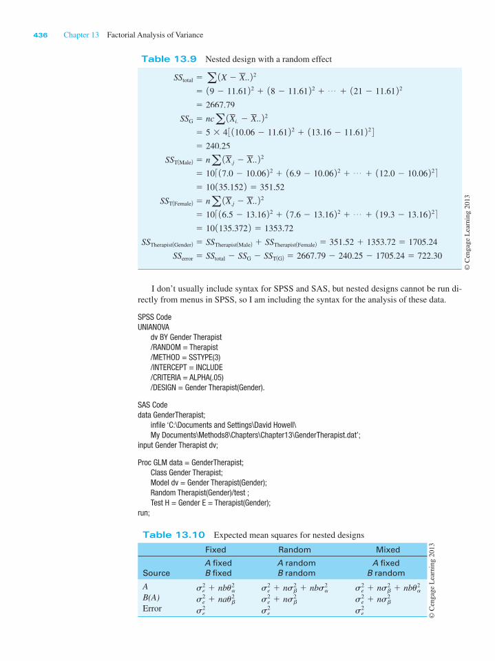
436 Chapter 13 Factorial Analysis of Variance
I don’t usually include syntax for SPSS and SAS, but nested designs cannot be run di-
rectly from menus in SPSS, so I am including the syntax for the analysis of these data.
SPSS CodeUNIANOVA
dv BY Gender Therapist/RANDOM = Therapist/METHOD = SSTYPE(3)/INTERCEPT = INCLUDE/CRITERIA = ALPHA(.05)/DESIGN = Gender Therapist(Gender).
SAS Codedata GenderTherapist;
infile ‘C:\Documents and Settings\David Howell\My Documents\Methods8\Chapters\Chapter13\GenderTherapist.dat’;
input Gender Therapist dv;
Proc GLM data = GenderTherapist;Class Gender Therapist;Model dv = Gender Therapist(Gender);Random Therapist(Gender)/test ;Test H = Gender E = Therapist(Gender);
run;
Table 13.10 Expected mean squares for nested designs
Fixed Random Mixed
Source
A fixed
B fixed
A random
B random
A fixed
B random
AB(A)Error
s2e 1 nbu2
a
s2e 1 nau2
b
s2e
s2e 1 ns2
b 1 nbs2a
s2e 1 ns2
b
s2e
s2e 1 ns2
b 1 nbu2a
s2e 1 ns2
b
s2e
Table 13.9 Nested design with a random effect
SStotal 5 a 1X 2 X.. 2 2 5 19 2 11.61 2 2 1 18 2 11.61 2 2 1 c 1 121 2 11.61 2 2 5 2667.79
SSG 5 nca 1Xi. 2 X.. 2 2 5 5 3 4 3 110.06 2 11.61 2 2 1 113.16 2 11.61 2 2 4 5 240.25
SST1Male2 5 na 1X.j 2 X.. 2 2 5 10 3 17.0 2 10.06 2 2 1 16.9 2 10.06 2 2 1 c 1 112.0 2 10.06 2 2 4 5 10 135.152 2 5 351.52
SST1Female2 5 na 1X.j 2 X.. 2 2 5 10 3 16.5 2 13.16 2 2 1 17.6 2 13.16 2 2 1 c 1 119.3 2 13.16 2 2 4 5 10 1135.372 2 5 1353.72
SSTherapist1Gender2 5 SSTherapist1Male2 1 SSTherapist1Female2 5 351.52 1 1353.72 5 1705.24
SSerror 5 SStotal 2 SSG 2 SST1G2 5 2667.79 2 240.25 2 1705.24 5 722.30
© C
engag
e L
earn
ing 2
013
© C
engag
e L
earn
ing 2
013

Section 13.9 Measures of Association and Effect Size 437
Notice in Table 13.10 that when we have a nested design with a random variable nested
within a fixed variable our F statistic is going to be computed differently. We can test the
effect of Therapist(Gender) by dividing MST(G) by MSerror, but when we want to test Gender
we must divide MSG by MST(G). The resulting Fs are shown in Table 13.11, where I have
subscripted the error terms to indicate how the Fs were constructed.
Notice that the Gender effect has the same sum of squares that it had in the origi-
nal study, but the F is quite different because Therapist(Gender) served as the error term
and there was considerable variability among therapists. Notice also that SSTherapist(Gender) is
equal to the sum of SSCondition and SSAge 3 Condition in the first example, although I prefer to
think of it as the sum of the two simple effects.
Having a random factor such as Therapist often creates a problem. We really set out to
study Gender differences, and that is what we most care about. We don’t really care much
about therapist differences because we know that they will be there. But the fact that Thera-
pist is a random effect, which it should be, dramatically altered our test on Gender. The F
went from nearly 30 to nearly 1.0. This is a clear case where the design of the study has
a dramatic effect on power, even with the same values for the data. Maxwell and Delaney
(2004) make the point that in designs with random factors, power depends on both the
number of subjects (here, clients) and the number of levels of the random variable (here,
therapists). Generally the number of levels of the random variable is far more important.
Summary
I have presented three experimental designs. The crossed design with fixed factors is the
workhorse for most traditional experimental studies. The nested design with a random fac-
tor is an important design in much research in education and more applied areas of psychol-
ogy. The crossed design with a random factor occurs occasionally but is not as common. In
general when you have crossed effects they are most often fixed, and when you have nested
effects the nested factor is most often random. This helps to explain why when you go to
other sources to look up nested (or random) designs you will often find the two discussed
together. A final point to keep in mind is that in all of the between-subjects designs in this
book, subjects are nested within other factors and are considered to be a random factor. All
of our F statistics are computed taking that into account.
13.9 Measures of Association and Effect Size
We can look at the magnitude of an effect in two different ways, just as we did with the
one-way analysis. We can either calculate an r-family measure, such as h2, or we can cal-
culate a d-family measure such as d. Normally when we are examining an omnibus F, we
use an r-family measure. However, when we are looking at a contrast between means, it is
usually more meaningful to calculate an effect size estimate (d). We have seen both types
of measures in previous chapters.
Table 13.11 Tests for a nested design with a random nested factor
Source df SS MS F
Gender
Error1
Therapist(Gender)
Error2
1
8
8
90
240.25
1705.24
1705.24
722.30
240.250
213.155
213.155
8.026
1.127
26.56*
Total 99 2667.79
* p , .05 © C
engag
e L
earn
ing 2
013
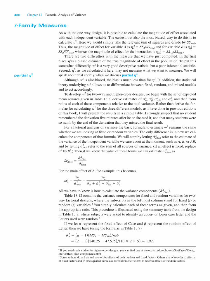
438 Chapter 13 Factorial Analysis of Variance
r-Family Measures
As with the one-way design, it is possible to calculate the magnitude of effect associated
with each independent variable. The easiest, but also the most biased, way to do this is to
calculate h2. Here we would simply take the relevant sum of squares and divide by SStotal.
Thus, the magnitude of effect for variable A is ha2 5 SSA/SStotal and for variable B is hb
2 5
SSB/SStotal, whereas the magnitude of effect for the interaction is hab2 5 SSAB/SStotal
.
There are two difficulties with the measure that we have just computed. In the first
place h2is a biased estimate of the true magnitude of effect in the population. To put this
somewhat differently, h2 is a very good descriptive statistic, but a poor inferential statistic.
Second, h2, as we calculated it here, may not measure what we want to measure. We will
speak about that shortly when we discuss partial h2.
Although v2 is also biased, the bias is much less than for h2. In addition, the statistical
theory underlying v2 allows us to differentiate between fixed, random, and mixed models
and to act accordingly.
To develop v2 for two-way and higher-order designs, we begin with the set of expected
mean squares given in Table 13.8, derive estimates of s2a, s2
b, s2ab, and s2
e, and then form
ratios of each of these components relative to the total variance. Rather than derive the for-
mulae for calculating v2 for the three different models, as I have done in previous editions
of this book, I will present the results in a simple table. I strongly suspect that no student
remembered the derivation five minutes after he or she read it, and that many students were
so numb by the end of the derivation that they missed the final result.
For a factorial analysis of variance the basic formula to estimate v2 remains the same
whether we are looking at fixed or random variables. The only difference is in how we cal-
culate the components of that formula. We will start by letting s2effect refer to the estimate of
the variance of the independent variable we care about at the moment, such as A, B, or AB,
and by letting s2total refer to the sum of all sources of variance. (If an effect is fixed, replace
s2 by u2.) Then if we know the value of these terms we can estimate v2effect as
v2effect 5
s2effect
s2total
For the main effect of A, for example, this becomes
v2a 5
s2a
s2total
5s2
a
s2a 1 s2
b 1 s2ab 1 s2
e
All we have to know is how to calculate the variance components 1 s2effect 2 .
Table 13.12 contains the variance components for fixed and random variables for two-
way factorial designs, where the subscripts in the leftmost column stand for fixed (f) or
random (r) variables.4 You simply calculate each of these terms as given, and then form
the appropriate ratio. This procedure is illustrated using the summary table from the design
in Table 13.8, where subjects were asked to identify an upper- or lower case letter and the
Letters used were random.5
If we let a represent the fixed effect of Case and b represent the random effect of
Letter, then we have (using the formulae in Table 13.9)
s2a 5 1a 2 1 2 1MSA 2 MSAB 2 /nab
5 12 2 1 2 1240.25 2 47.575 2 / 110 3 2 3 5 2 5 1.927
partial h2
4 If you need such a table for higher-order designs, you can find one at www.uvm.edu/~dhowell/StatPages/More_
Stuff/Effect_size_components.html5 Some authors do as I do and use v2 for effects of both random and fixed factors. Others use v2 to refer to effects
of fixed factors and r2 (the squared intraclass correlation coefficient) to refer to effects of random factors.
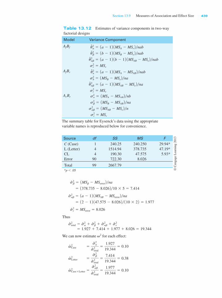
Section 13.9 Measures of Association and Effect Size 439
s2b 5 1MSb 2 MSerror 2 /na
5 1378.735 2 8.026 2 /10 3 5 5 7.414
s2ab 5 1a 2 1 2 1MSAB 2 MSerror 2 /na
5 12 2 1 2 147.575 2 8.026 2 / 110 3 2 2 5 1.977
s2e 5 MSerror 5 8.026
Thus
s2total 5 s2
a 1 s2b 1 s2
ab 1 s2e
5 1.927 1 7.414 1 1.977 1 8.026 5 19.344
We can now estimate v2 for each effect:
v2Case 5
s2a
s2total
51.927
19.3445 0.10
v2Letter 5
s2b
s2total
57.414
19.3445 0.38
v2Case3Letter 5
s2ab
s2total
51.977
19.3445 0.10
Table 13.12 Estimates of variance components in two-way
factorial designs
Model Variance Component
Af Bf u2a 5 1a 2 1 2 1MSA 2 MSe 2 /nab
u2b 5 1b 2 1 2 1MSB 2 MSe 2 /nab
u2ab 5 1a 2 1 2 1b 2 1 2 1MSAB 2 MSe 2 /nab
s2e 5 MSe
Af Br u2a 5 1a 2 1 2 1MSA 2 MSAB 2 /nab
s2b 5 1MSB 2 MSe 2 /na
u2ab 5 1a 2 1 2 1MSAB 2 MSe 2 /na
s2e 5 MSe
Ar Br s2a 5 1MSA 2 MSAB 2 /nb
s2b 5 1MSB 2 MSAB 2 /na
s2ab 5 1MSAB 2 MSe 2 /n s2
e 5 MSe
The summary table for Eysenck’s data using the appropriate
variable names is reproduced below for convenience.
Source df SS MS F
C (Case) 1 240.25 240.250 29.94*
L (Letter) 4 1514.94 378.735 47.19*
CL 4 190.30 47.575 5.93*
Error 90 722.30 8.026
Total 99 2667.79
*p , .05 © C
engag
e L
earn
ing 2
013
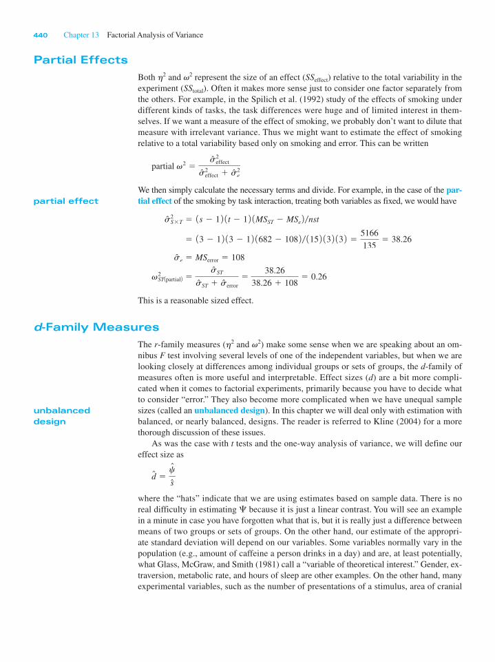
440 Chapter 13 Factorial Analysis of Variance
Partial Effects
Both h2 and v2 represent the size of an effect (SSeffect) relative to the total variability in the
experiment (SStotal). Often it makes more sense just to consider one factor separately from
the others. For example, in the Spilich et al. (1992) study of the effects of smoking under
different kinds of tasks, the task differences were huge and of limited interest in them-
selves. If we want a measure of the effect of smoking, we probably don’t want to dilute that
measure with irrelevant variance. Thus we might want to estimate the effect of smoking
relative to a total variability based only on smoking and error. This can be written
partial v2 5s2
effect
s2effect 1 s2
e
We then simply calculate the necessary terms and divide. For example, in the case of the par-tial effect of the smoking by task interaction, treating both variables as fixed, we would have
s2S3T 5 1s 2 1 2 1 t 2 1 2 1MSST 2 MSe 2 /nst
5 13 2 1 2 13 2 1 2 1682 2 108 2 / 115 2 13 2 13 2 55166
1355 38.26
se 5 MSerror 5 108
v2ST1partial2 5
sST
sST 1 serror
538.26
38.26 1 1085 0.26
This is a reasonable sized effect.
d-Family Measures
The r-family measures (h2 and v2) make some sense when we are speaking about an om-
nibus F test involving several levels of one of the independent variables, but when we are
looking closely at differences among individual groups or sets of groups, the d-family of
measures often is more useful and interpretable. Effect sizes (d) are a bit more compli-
cated when it comes to factorial experiments, primarily because you have to decide what
to consider “error.” They also become more complicated when we have unequal sample
sizes (called an unbalanced design). In this chapter we will deal only with estimation with
balanced, or nearly balanced, designs. The reader is referred to Kline (2004) for a more
thorough discussion of these issues.
As was the case with t tests and the one-way analysis of variance, we will define our
effect size as
d 5c
s
where the “hats” indicate that we are using estimates based on sample data. There is no
real difficulty in estimating C because it is just a linear contrast. You will see an example
in a minute in case you have forgotten what that is, but it is really just a difference between
means of two groups or sets of groups. On the other hand, our estimate of the appropri-
ate standard deviation will depend on our variables. Some variables normally vary in the
population (e.g., amount of caffeine a person drinks in a day) and are, at least potentially,
what Glass, McGraw, and Smith (1981) call a “variable of theoretical interest.” Gender, ex-
traversion, metabolic rate, and hours of sleep are other examples. On the other hand, many
experimental variables, such as the number of presentations of a stimulus, area of cranial
partial effect
unbalanced
design
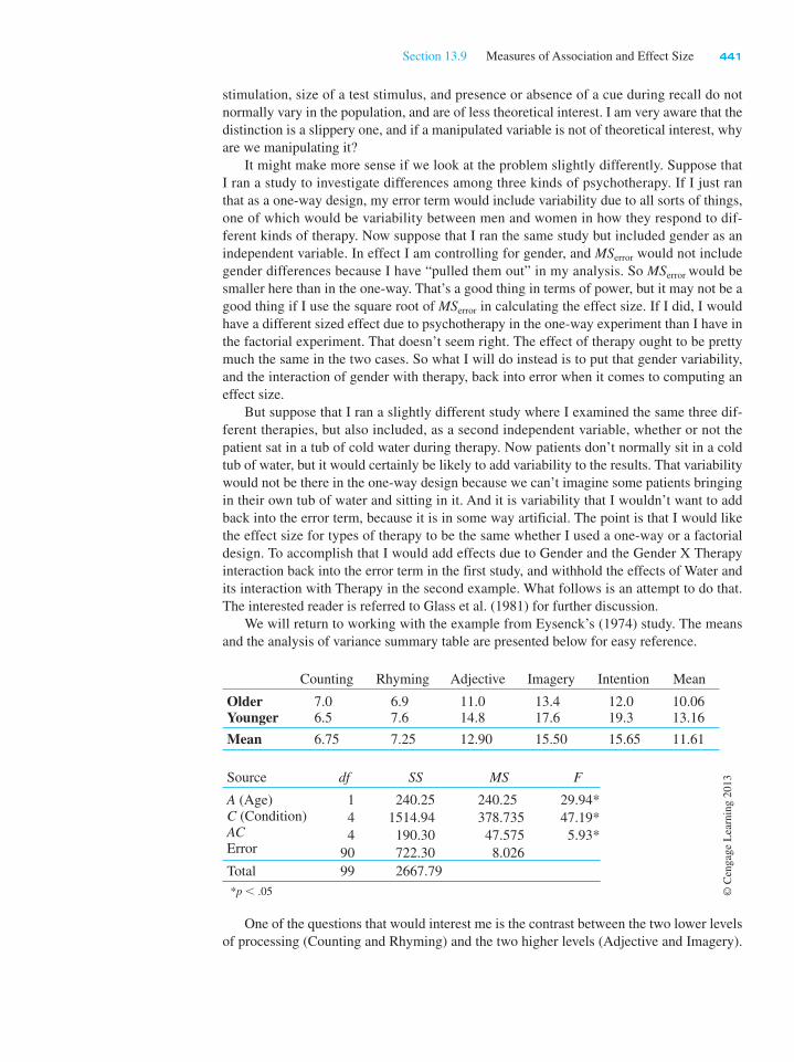
Section 13.9 Measures of Association and Effect Size 441
stimulation, size of a test stimulus, and presence or absence of a cue during recall do not
normally vary in the population, and are of less theoretical interest. I am very aware that the
distinction is a slippery one, and if a manipulated variable is not of theoretical interest, why
are we manipulating it?
It might make more sense if we look at the problem slightly differently. Suppose that
I ran a study to investigate differences among three kinds of psychotherapy. If I just ran
that as a one-way design, my error term would include variability due to all sorts of things,
one of which would be variability between men and women in how they respond to dif-
ferent kinds of therapy. Now suppose that I ran the same study but included gender as an
independent variable. In effect I am controlling for gender, and MSerror would not include
gender differences because I have “pulled them out” in my analysis. So MSerror would be
smaller here than in the one-way. That’s a good thing in terms of power, but it may not be a
good thing if I use the square root of MSerror in calculating the effect size. If I did, I would
have a different sized effect due to psychotherapy in the one-way experiment than I have in
the factorial experiment. That doesn’t seem right. The effect of therapy ought to be pretty
much the same in the two cases. So what I will do instead is to put that gender variability,
and the interaction of gender with therapy, back into error when it comes to computing an
effect size.
But suppose that I ran a slightly different study where I examined the same three dif-
ferent therapies, but also included, as a second independent variable, whether or not the
patient sat in a tub of cold water during therapy. Now patients don’t normally sit in a cold
tub of water, but it would certainly be likely to add variability to the results. That variability
would not be there in the one-way design because we can’t imagine some patients bringing
in their own tub of water and sitting in it. And it is variability that I wouldn’t want to add
back into the error term, because it is in some way artificial. The point is that I would like
the effect size for types of therapy to be the same whether I used a one-way or a factorial
design. To accomplish that I would add effects due to Gender and the Gender X Therapy
interaction back into the error term in the first study, and withhold the effects of Water and
its interaction with Therapy in the second example. What follows is an attempt to do that.
The interested reader is referred to Glass et al. (1981) for further discussion.
We will return to working with the example from Eysenck’s (1974) study. The means
and the analysis of variance summary table are presented below for easy reference.
Counting Rhyming Adjective Imagery Intention Mean
OlderYounger
7.0
6.5
6.9
7.6
11.0
14.8
13.4
17.6
12.0
19.3
10.06
13.16
Mean 6.75 7.25 12.90 15.50 15.65 11.61
Source df SS MS F
A (Age)
C (Condition)
ACError
1
4
4
90
240.25
1514.94
190.30
722.30
240.25
378.735
47.575
8.026
29.94*
47.19*
5.93*
Total 99 2667.79
*p , .05
One of the questions that would interest me is the contrast between the two lower levels
of processing (Counting and Rhyming) and the two higher levels (Adjective and Imagery).
© C
engag
e L
earn
ing 2
013
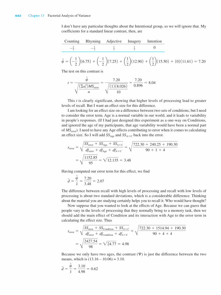
442 Chapter 13 Factorial Analysis of Variance
I don’t have any particular thoughts about the Intentional group, so we will ignore that. My
coefficients for a standard linear contrast, then, are
Counting Rhyming Adjective Imagery Intention
212 2
12
12
12
0
c 5 a21
2 b 16.75 2 1 a21
2 b 17.25 2 1 a1
2b 112.90 2 1 a1
2b 115.50 2 1 10 2 111.61 2 5 7.20
The test on this contrast is
t 5c
Å 1Sa2i 2MSerror
n
57.20
Å 11 2 18.026 210
57.20
0.8965 8.04
This t is clearly significant, showing that higher levels of processing lead to greater
levels of recall. But I want an effect size for this difference.
I am looking for an effect size on a difference between two sets of conditions, but I need
to consider the error term. Age is a normal variable in our world, and it leads to variability
in people’s responses. (If I had just designed this experiment as a one-way on Conditions,
and ignored the age of my participants, that age variability would have been a normal part
of MSerror). I need to have any Age effects contributing to error when it comes to calculating
an effect size. So I will add SSAge and SSA 3 C back into the error.
serror 5 ÅSSerror 1 SSAge 1 SSA3C
dferror 1 dfAge 1 dfA3C
5 Å722.30 1 240.25 1 190.30
90 1 1 1 4
5 Å1152.85
955 "12.135 5 3.48
Having computed our error term for this effect, we find
d 5c
s5
7.20
3.485 2.07
The difference between recall with high levels of processing and recall with low levels of
processing is about two standard deviations, which is a considerable difference. Thinking
about the material you are studying certainly helps you to recall it. Who would have thought?
Now suppose that you wanted to look at the effects of Age. Because we can guess that
people vary in the levels of processing that they normally bring to a memory task, then we
should add the main effect of Condition and its interaction with Age to the error term in
calculating the effect size. Thus
serror 5 ÅSSerror 1 SSCondition 1 SSA3C
dferror 1 dfCondition 1 dfA3C
5 Å722.30 1 1514.94 1 190.30
90 1 4 1 4
5 Å2427.54
985 "24.77 5 4.98
Because we only have two ages, the contrast (C) is just the difference between the two
means, which is (13.16 – 10.06) = 3.10.
d 5c
s5
3.10
4.985 0.62

Section 13.10 Reporting the Results 443
In this case younger subjects differ from older participants by nearly two-thirds of a stand-
ard deviation.
Simple Effects
The effect sizes for simple effects are calculated in ways directly derived from the way we
calculate main effects. The error term in these calculations is the same error term as that
used for the corresponding main effect. Thus for the simple effect of Age for highest level
of processing (Imagery) is
d 5c
s5117.6 2 13.4 2
4.985
4.20
4.985 0.84
Similarly, for the contrast of low levels of processing versus high levels among young par-
ticipants we would have
c 5 a21
2b 16.5 2 1 a21
2b 17.6 2 1 a1
2b 114.8 2 1 a1
2b 117.6 2 1 10 2 119.3 2 5 9.15
and the effect size is
d 5c
s5
9.15
3.485 2.63
which means that for younger participants there is nearly a 22/3 standard deviation differ-
ence in recall between the high and low levels of processing.
13.10 Reporting the Results
We have carried out a number of calculations to make various points, and I would certainly
not report all of them when writing up the results. What follows is the basic information
that I think needs to be presented.
In an investigation of the effects of different levels of information processing on the re-
tention of verbal material, participants were instructed to process verbal material in one
of four ways, ranging from the simple counting of letters in words to forming a visual
image of each word. Participants in a fifth condition were not given any instructions
about what to do with the items other than to study them for later recall. A second di-
mension of the experiment compared Younger and Older participants in terms of recall,
thus forming a 2 3 5 factorial design.
The dependent variable was the number of items recalled after three presentations of
the material. There was a significant Age effect (F(1,90) 5 29.94, p , .05, v2 5 .087),
with younger participants recalling more items than older ones. There was also a signifi-
cant effect due to Condition (F(4,90) 5 47.19, p , .05, v2 5 .554), and visual inspection
of the means shows that there was greater recall for conditions in which there was a greater
degree of processing. Finally the Age by Condition interaction was significant (F(4,90) 5
5.93, p , .05, v2 5 .059), with a stronger effect of Condition for the younger participants.
A contrast of lower levels of processing (Counting and Rhyming) with higher levels
of processing (Adjective and Imagery) produced a clearly statistically significant effect
in favor of higher levels of processing 1 t 190 2 5 8.04, p , .05 2 . This corresponds to
an effect size of d 5 2.07, indicating that participants with higher levels of processing
outperform those with lower levels of processing by over two standard deviations. This
effect is even greater if we look only at the younger participants, where d 5 2.63.

444 Chapter 13 Factorial Analysis of Variance
13.11 Unequal Sample Sizes
Although many (but certainly not all) experiments are designed with the intention of hav-
ing equal numbers of observations in each cell, the cruel hand of fate frequently intervenes
to upset even the most carefully laid plans. Participants fail to arrive for testing, animals
die, data are lost, apparatus fails, patients drop out of treatment, and so on. When such
problems arise, we are faced with several alternative solutions, with the choice depending
on the nature of the data and the reasons why data are missing.
When we have a plain one-way analysis of variance, the solution is simple and we have
already seen how to carry that out. When we have more complex designs, the solution is
not simple. With unequal sample sizes in factorial designs, the row, column, and interaction
effects are no longer independent. This lack of independence produces difficulties in inter-
pretation, and deciding on the best approach depends both on why the data are missing and
how we conceive of our model.
There has been a great deal written about the treatment of unequal sample sizes, and we
won’t see any true resolution of this issue for a long time. (That is in part because there is
no single answer to the complex questions that arise.) However, there are some approaches
that seem more reasonable than others for the general case. Unfortunately, the most reason-
able and the most common approach is available only using standard computer packages,
and a discussion of that will have to wait until Chapter 15. I will, however, describe a
pencil-and-paper solution to illustrate how we might think of the analysis. (I don’t expect
that you would actually use this approach in calculation, but it nicely illustrates some of
the issues and helps to understand what SPSS are most other programs are doing.) This ap-
proach is commonly referred to as an unweighted means solution or an equally weighted means solution because we weight the cell means equally, regardless of the number of
observations in those cells. My primary purpose in discussing this approach is not to make
you get out your pencil and a calculator, but to help provide an understanding of what
SPSS and SAS do if you take the default options. Although I will not work out an example,
such an example can be found in Exercise 13.16. And, if you have difficulty with that, the
solution can be found online in the Student Manual (www.uvm.edu/~dhowell/methods8
/StudentManual/StudentManual.html).
The Problem
You can see what our problem is if we take a very simple 2 3 2 factorial where we know
what is happening. Suppose that we propose to test vigilance on a simple driving task when
participants are either sober or are under the influence of alcohol. The task involves using
a driving simulator and having participants respond when cars suddenly come out of drive-
ways and when pedestrians suddenly step into the street. We would probably expect that
sober drivers would make many fewer errors on this task than drivers who had been plied
with alcohol. We will have two investigators working together on this problem, one from
Michigan and one from Arizona, and each of them will run about half of the participants in
their own facilities. We have absolutely no reason to believe that participants in Michigan
are any different from participants in Arizona, nor do we have any reason to believe that
there would be a significant interaction between State and Alcohol condition, though a plot
of the data would be unlikely to show lines that are exactly parallel. I constructed the data
with those expectations in mind.
Suppose that we obtained the quite extreme data shown in Table 13.13 with unequal
numbers of participants in the four cells. The dependent variable is the number of errors
each driver made in one half-hour session. From the cell means in this table you can see
unweighted
means
equally weighted
means
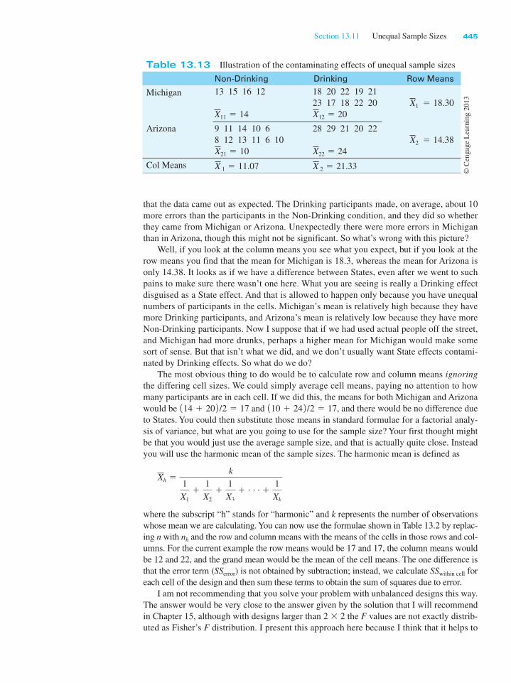
Section 13.11 Unequal Sample Sizes 445
that the data came out as expected. The Drinking participants made, on average, about 10
more errors than the participants in the Non-Drinking condition, and they did so whether
they came from Michigan or Arizona. Unexpectedly there were more errors in Michigan
than in Arizona, though this might not be significant. So what’s wrong with this picture?
Well, if you look at the column means you see what you expect, but if you look at the
row means you find that the mean for Michigan is 18.3, whereas the mean for Arizona is
only 14.38. It looks as if we have a difference between States, even after we went to such
pains to make sure there wasn’t one here. What you are seeing is really a Drinking effect
disguised as a State effect. And that is allowed to happen only because you have unequal
numbers of participants in the cells. Michigan’s mean is relatively high because they have
more Drinking participants, and Arizona’s mean is relatively low because they have more
Non-Drinking participants. Now I suppose that if we had used actual people off the street,
and Michigan had more drunks, perhaps a higher mean for Michigan would make some
sort of sense. But that isn’t what we did, and we don’t usually want State effects contami-
nated by Drinking effects. So what do we do?
The most obvious thing to do would be to calculate row and column means ignoring
the differing cell sizes. We could simply average cell means, paying no attention to how
many participants are in each cell. If we did this, the means for both Michigan and Arizona
would be 114 1 20 2 /2 5 17 and 110 1 24 2 /2 5 17, and there would be no difference due
to States. You could then substitute those means in standard formulae for a factorial analy-
sis of variance, but what are you going to use for the sample size? Your first thought might
be that you would just use the average sample size, and that is actually quite close. Instead
you will use the harmonic mean of the sample sizes. The harmonic mean is defined as
Xh 5k
1
X1
11
X2
11
X3
1 c11
Xk
where the subscript “h” stands for “harmonic” and k represents the number of observations
whose mean we are calculating. You can now use the formulae shown in Table 13.2 by replac-
ing n with nh and the row and column means with the means of the cells in those rows and col-
umns. For the current example the row means would be 17 and 17, the column means would
be 12 and 22, and the grand mean would be the mean of the cell means. The one difference is
that the error term (SSerror) is not obtained by subtraction; instead, we calculate SSwithin cell for
each cell of the design and then sum these terms to obtain the sum of squares due to error.
I am not recommending that you solve your problem with unbalanced designs this way.
The answer would be very close to the answer given by the solution that I will recommend
in Chapter 15, although with designs larger than 2 3 2 the F values are not exactly distrib-
uted as Fisher’s F distribution. I present this approach here because I think that it helps to
Table 13.13 Illustration of the contaminating effects of unequal sample sizes
Non-Drinking Drinking Row Means
Michigan 13 15 16 12
X11 5 14
18 20 22 19 21
23 17 18 22 20
X12 5 20
X1. 5 18.30
Arizona 9 11 14 10 6
8 12 13 11 6 10
X21 5 10
28 29 21 20 22
X22 5 24
X2. 5 14.38
Col Means X.1 5 11.07 X.2 5 21.33
© C
engag
e L
earn
ing 2
013
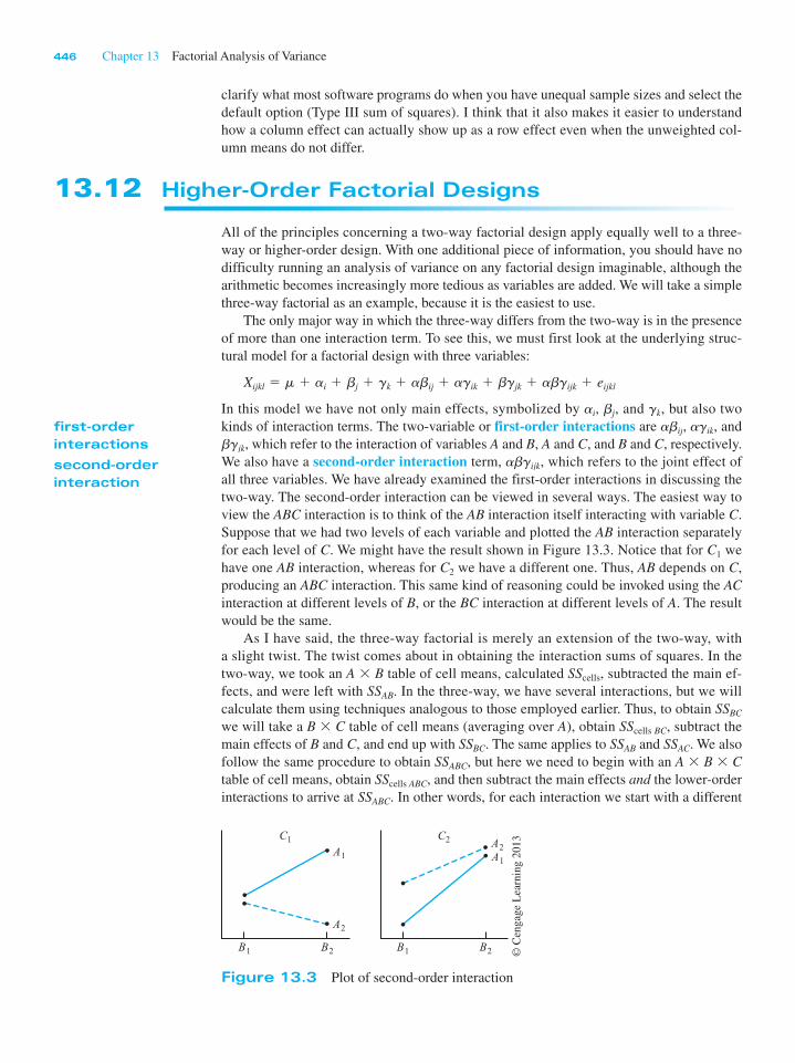
446 Chapter 13 Factorial Analysis of Variance
clarify what most software programs do when you have unequal sample sizes and select the
default option (Type III sum of squares). I think that it also makes it easier to understand
how a column effect can actually show up as a row effect even when the unweighted col-
umn means do not differ.
13.12 Higher-Order Factorial Designs
All of the principles concerning a two-way factorial design apply equally well to a three-
way or higher-order design. With one additional piece of information, you should have no
difficulty running an analysis of variance on any factorial design imaginable, although the
arithmetic becomes increasingly more tedious as variables are added. We will take a simple
three-way factorial as an example, because it is the easiest to use.
The only major way in which the three-way differs from the two-way is in the presence
of more than one interaction term. To see this, we must first look at the underlying struc-
tural model for a factorial design with three variables:
Xijkl 5 m 1 ai 1 bj 1 gk 1 abij 1 agik 1 bgjk 1 abgijk 1 eijkl
In this model we have not only main effects, symbolized by ai, bj, and gk, but also two
kinds of interaction terms. The two-variable or first-order interactions are abij, agik, and
bgjk, which refer to the interaction of variables A and B, A and C, and B and C, respectively.
We also have a second-order interaction term, abgijk, which refers to the joint effect of
all three variables. We have already examined the first-order interactions in discussing the
two-way. The second-order interaction can be viewed in several ways. The easiest way to
view the ABC interaction is to think of the AB interaction itself interacting with variable C.
Suppose that we had two levels of each variable and plotted the AB interaction separately
for each level of C. We might have the result shown in Figure 13.3. Notice that for C1 we
have one AB interaction, whereas for C2 we have a different one. Thus, AB depends on C,
producing an ABC interaction. This same kind of reasoning could be invoked using the AC
interaction at different levels of B, or the BC interaction at different levels of A. The result
would be the same.
As I have said, the three-way factorial is merely an extension of the two-way, with
a slight twist. The twist comes about in obtaining the interaction sums of squares. In the
two-way, we took an A 3 B table of cell means, calculated SScells, subtracted the main ef-
fects, and were left with SSAB. In the three-way, we have several interactions, but we will
calculate them using techniques analogous to those employed earlier. Thus, to obtain SSBC
we will take a B 3 C table of cell means (averaging over A), obtain SScells BC, subtract the
main effects of B and C, and end up with SSBC. The same applies to SSAB and SSAC. We also
follow the same procedure to obtain SSABC, but here we need to begin with an A 3 B 3 C
table of cell means, obtain SScells ABC, and then subtract the main effects and the lower-order
interactions to arrive at SSABC. In other words, for each interaction we start with a different
first-order
interactions
second-order
interaction
B2
C1A1
A2
B1 B2
C2
A1
A2
B1
Figure 13.3 Plot of second-order interaction
© C
engag
e L
earn
ing 2
013
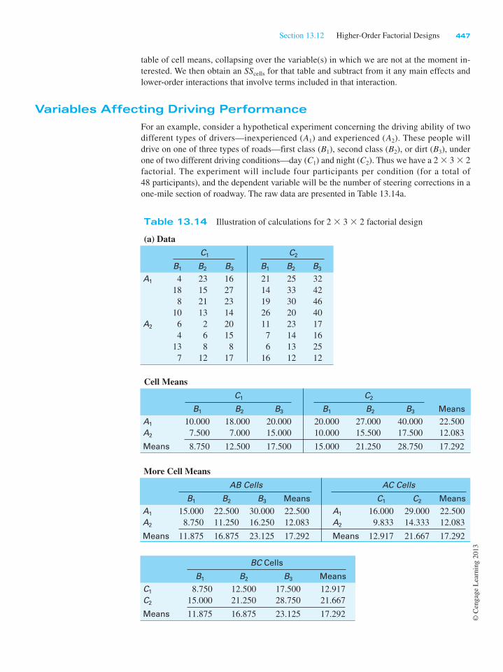
Section 13.12 Higher-Order Factorial Designs 447
table of cell means, collapsing over the variable(s) in which we are not at the moment in-
terested. We then obtain an SScells for that table and subtract from it any main effects and
lower-order interactions that involve terms included in that interaction.
Variables Affecting Driving Performance
For an example, consider a hypothetical experiment concerning the driving ability of two
different types of drivers—inexperienced (A1) and experienced (A2). These people will
drive on one of three types of roads—first class (B1), second class (B2), or dirt (B3), under
one of two different driving conditions—day (C1) and night (C2). Thus we have a 2 3 3 3 2
factorial. The experiment will include four participants per condition (for a total of
48 participants), and the dependent variable will be the number of steering corrections in a
one-mile section of roadway. The raw data are presented in Table 13.14a.
Table 13.14 Illustration of calculations for 2 3 3 3 2 factorial design
(a) Data
C1 C2
B1 B2 B3 B1 B2 B3
A1 4 23 16 21 25 32
18 15 27 14 33 42
8 21 23 19 30 46
10 13 14 26 20 40
A2 6 2 20 11 23 17
4 6 15 7 14 16
13 8 8 6 13 25
7 12 17 16 12 12
Cell Means
C1 C2
B1 B2 B3 B1 B2 B3 Means
A1 10.000 18.000 20.000 20.000 27.000 40.000 22.500
A2 7.500 7.000 15.000 10.000 15.500 17.500 12.083
Means 8.750 12.500 17.500 15.000 21.250 28.750 17.292
More Cell Means
AB Cells AC Cells
B1 B2 B3 Means C1 C2 Means
A1 15.000 22.500 30.000 22.500 A1 16.000 29.000 22.500
A2 8.750 11.250 16.250 12.083 A2 9.833 14.333 12.083
Means 11.875 16.875 23.125 17.292 Means 12.917 21.667 17.292
BC Cells
B1 B2 B3 Means
C1 8.750 12.500 17.500 12.917
C2 15.000 21.250 28.750 21.667
Means 11.875 16.875 23.125 17.292
© C
engag
e L
earn
ing 2
013
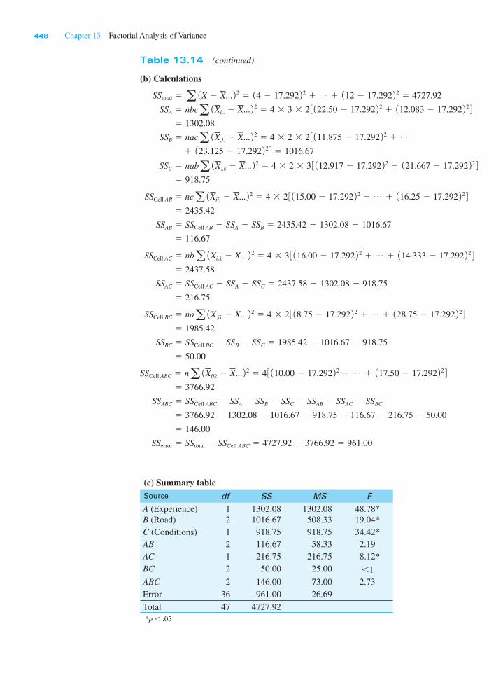
448 Chapter 13 Factorial Analysis of Variance
(b) Calculations
SStotal 5 a 1X 2 X... 2 2 5 14 2 17.292 2 2 1 c 1 112 2 17.292 2 2 5 4727.92
SSA 5 nbca 1Xi.. 2 X... 2 2 5 4 3 3 3 2 3 122.50 2 17.292 2 2 1 112.083 2 17.292 2 2 4 5 1302.08
SSB 5 naca 1X.j. 2 X... 2 2 5 4 3 2 3 2 3 111.875 2 17.292 2 2 1 c
1 123.125 2 17.292 2 2 4 5 1016.67
SSC 5 naba 1X..k 2 X... 2 2 5 4 3 2 3 3 3 112.917 2 17.292 2 2 1 121.667 2 17.292 2 2 4 5 918.75
SSCell AB 5 nca 1Xij. 2 X... 2 2 5 4 3 2 3 115.00 2 17.292 2 2 1 c 1 116.25 2 17.292 2 2 4 5 2435.42
SSAB 5 SSCell AB 2 SSA 2 SSB 5 2435.42 2 1302.08 2 1016.67
5 116.67
SSCell AC 5 nba 1Xi.k 2 X... 2 2 5 4 3 3 3 116.00 2 17.292 2 2 1 c 1 114.333 2 17.292 2 2 4 5 2437.58
SSAC 5 SSCell AC 2 SSA 2 SSC 5 2437.58 2 1302.08 2 918.75
5 216.75
SSCell BC 5 naa 1X.jk 2 X... 2 2 5 4 3 2 3 18.75 2 17.292 2 2 1 c 1 128.75 2 17.292 2 2 4 5 1985.42
SSBC 5 SSCell BC 2 SSB 2 SSC 5 1985.42 2 1016.67 2 918.75
5 50.00
SSCell ABC 5 na 1Xijk 2 X... 2 2 5 4 3 110.00 2 17.292 2 2 1 c 1 117.50 2 17.292 2 2 4 5 3766.92
SSABC 5 SSCell ABC 2 SSA 2 SSB 2 SSC 2 SSAB 2 SSAC 2 SSBC
5 3766.92 2 1302.08 2 1016.67 2 918.75 2 116.67 2 216.75 2 50.00
5 146.00
SSerror 5 SStotal 2 SSCell ABC 5 4727.92 2 3766.92 5 961.00
(c) Summary tableSource df SS MS F
A (Experience) 1 1302.08 1302.08 48.78*
B (Road) 2 1016.67 508.33 19.04*
C (Conditions) 1 918.75 918.75 34.42*
AB 2 116.67 58.33 2.19
AC 1 216.75 216.75 8.12*
BC 2 50.00 25.00 ,1
ABC 2 146.00 73.00 2.73
Error 36 961.00 26.69
Total 47 4727.92
*p , .05
Table 13.14 (continued)
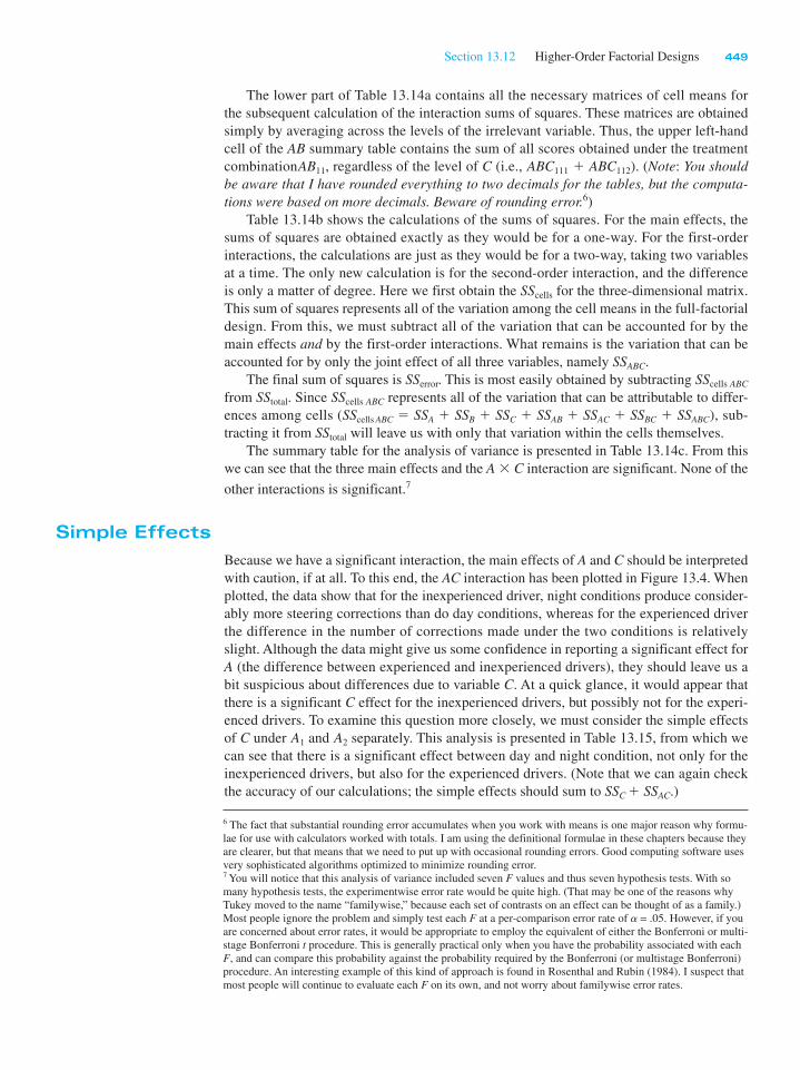
Section 13.12 Higher-Order Factorial Designs 449
The lower part of Table 13.14a contains all the necessary matrices of cell means for
the subsequent calculation of the interaction sums of squares. These matrices are obtained
simply by averaging across the levels of the irrelevant variable. Thus, the upper left-hand
cell of the AB summary table contains the sum of all scores obtained under the treatment
combinationAB11, regardless of the level of C (i.e., ABC111 1 ABC112). (Note: You should be aware that I have rounded everything to two decimals for the tables, but the computa-tions were based on more decimals. Beware of rounding error.6)
Table 13.14b shows the calculations of the sums of squares. For the main effects, the
sums of squares are obtained exactly as they would be for a one-way. For the first-order
interactions, the calculations are just as they would be for a two-way, taking two variables
at a time. The only new calculation is for the second-order interaction, and the difference
is only a matter of degree. Here we first obtain the SScells for the three-dimensional matrix.
This sum of squares represents all of the variation among the cell means in the full-factorial
design. From this, we must subtract all of the variation that can be accounted for by the
main effects and by the first-order interactions. What remains is the variation that can be
accounted for by only the joint effect of all three variables, namely SSABC.
The final sum of squares is SSerror. This is most easily obtained by subtracting SScells ABC
from SStotal. Since SScells ABC represents all of the variation that can be attributable to differ-
ences among cells (SScells ABC 5 SSA 1 SSB 1 SSC 1 SSAB 1 SSAC 1 SSBC 1 SSABC), sub-
tracting it from SStotal will leave us with only that variation within the cells themselves.
The summary table for the analysis of variance is presented in Table 13.14c. From this
we can see that the three main effects and the A 3 C interaction are significant. None of the
other interactions is significant.7
Simple Effects
Because we have a significant interaction, the main effects of A and C should be interpreted
with caution, if at all. To this end, the AC interaction has been plotted in Figure 13.4. When
plotted, the data show that for the inexperienced driver, night conditions produce consider-
ably more steering corrections than do day conditions, whereas for the experienced driver
the difference in the number of corrections made under the two conditions is relatively
slight. Although the data might give us some confidence in reporting a significant effect for
A (the difference between experienced and inexperienced drivers), they should leave us a
bit suspicious about differences due to variable C. At a quick glance, it would appear that
there is a significant C effect for the inexperienced drivers, but possibly not for the experi-
enced drivers. To examine this question more closely, we must consider the simple effects
of C under A1 and A2 separately. This analysis is presented in Table 13.15, from which we
can see that there is a significant effect between day and night condition, not only for the
inexperienced drivers, but also for the experienced drivers. (Note that we can again check
the accuracy of our calculations; the simple effects should sum to SSC 1 SSAC.)
6 The fact that substantial rounding error accumulates when you work with means is one major reason why formu-
lae for use with calculators worked with totals. I am using the definitional formulae in these chapters because they
are clearer, but that means that we need to put up with occasional rounding errors. Good computing software uses
very sophisticated algorithms optimized to minimize rounding error.7 You will notice that this analysis of variance included seven F values and thus seven hypothesis tests. With so
many hypothesis tests, the experimentwise error rate would be quite high. (That may be one of the reasons why
Tukey moved to the name “familywise,” because each set of contrasts on an effect can be thought of as a family.)
Most people ignore the problem and simply test each F at a per-comparison error rate of a = .05. However, if you
are concerned about error rates, it would be appropriate to employ the equivalent of either the Bonferroni or multi-
stage Bonferroni t procedure. This is generally practical only when you have the probability associated with each
F, and can compare this probability against the probability required by the Bonferroni (or multistage Bonferroni)
procedure. An interesting example of this kind of approach is found in Rosenthal and Rubin (1984). I suspect that
most people will continue to evaluate each F on its own, and not worry about familywise error rates.
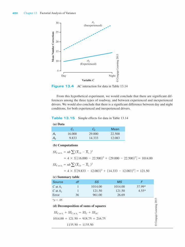
450 Chapter 13 Factorial Analysis of Variance
From this hypothetical experiment, we would conclude that there are significant dif-
ferences among the three types of roadway, and between experienced and inexperienced
drivers. We would also conclude that there is a significant difference between day and night
conditions, for both experienced and inexperienced drivers.
5
Day Night
Variable C
10
15
A1(Inexperienced)
A2(Experienced)
Mea
n N
umbe
r C
orre
ctio
ns
20
25
30
Figure 13.4 AC interaction for data in Table 13.14
Table 13.15 Simple effects for data in Table 13.14
(a) Data
C1 C2 Mean
A1 16.000 29.000 22.500
A2 9.833 14.333 12.083
(b) Computations
SSC at A15 nba 1X1.k 2 X1.. 2 2 5 4 3 3 3 116.000 2 22.500 2 2 1 129.000 2 22.500 2 2 4 5 1014.00
SSC at A25 nba 1X2.k 2 X2.. 2 2 5 4 3 3 3 19.833 2 12.083 2 2 1 114.333 2 12.083 2 2 4 5 121.50
(c) Summary table
Source df SS MS F
C at A1 1 1014.00 1014.00 37.99*
C at A2 1 121.50 121.50 4.55*
Error 36 961.00 26.69
*p , .05
(d) Decomposition of sums of squares
SSC at A11 SSC at A2
5 SSC 1 SSAC
1014.00 1 121.50 5 918.75 1 216.75
1135.50 5 1135.50
© C
engag
e L
earn
ing 2
013
© C
engag
e L
earn
ing 2
013
Section 13.13 A Computer Example 451
Simple Interaction Effects
With higher-order factorials, not only can we look at the effects of one variable at individual
levels of some other variable (what we have called simple effects but what should more accu-
rately be called simple main effects), but we can also look at the interaction of two variables at
individual levels of some third variable. This we will refer to as a simple interaction effect. Basically simple interaction effects are obtained in the same we that we obtain simple
main effects. We just use the data for one level of a variable at a time. Thus if we wanted to
look at the simple AB interactions in our example, we would take the data separately for C1
and C2 and treat those as two two-way analyses. I won’t work an example because it should
be apparent what you will do.
Although there is nothing to prevent someone from examining simple interaction effects
in the absence of a significant higher-order interaction, cases for which this would make any
logical sense are rare. If, however, the experimenter has a particular reason for looking at,
for example, the AB interaction at each level of C, he is perfectly free to do so. On the other
hand, if a higher-order interaction is significant, the experimenter should cast a wary eye on
all lower-order effects and consider testing the important simple effects. However, to steal a
line from Winer (1971, p. 442), “Statistical elegance does not necessarily imply scientifically
meaningful inferences.” Common sense is at least as important as statistical manipulations.
13.13 A Computer Example
The following example illustrates the analysis of a three-way factorial design with unequal
numbers of participants in the different cells. It is roughly based on a study by Seligman,
Nolen-Hoeksema, Thornton, and Thornton (1990), although the data are contrived and one
of the independent variables (Event) is fictitious. The main conclusions of the example are
in line with the results reported. Note that we will not discuss how SPSS and other pro-
grams handle unequal sample sizes in this example until we come to Chapter 15.
The study involved collegiate swimming teams. At a team practice, all participants were
asked to swim their best event as fast as possible, but in each case the time that was reported was
falsified to indicate poorer than expected performance. Thus each swimmer was disappointed at
receiving a poor result. Half an hour later, each swimmer was asked to perform the same event,
and their times were again recorded. The authors predicted that on the second trial more pessi-
mistic swimmers would do worse than on their first trial, whereas optimists would do better.
Participants were classified by their explanatory Style (optimism vs. pessimism), Sex, and
the preferred Event. The dependent variable was the ratio ofTime1/Time2, so a value greater
than 1.00 means that the swimmer did better on the second trial. The data and results are given
in Table 13.16. The results were obtained using SPSS. In examining the results remember that
SPSS prints several lines of output that we rarely care about, and they can just be ignored.
From the SPSS computer output you can see that there is a significant effect due to the
attributional style, with Optimists showing slightly improved performance after a perceived
failure, and pessimists doing worse. The difference in means may appear to be small, but
when you consider how close a race of this type usually is, even a tiny difference is impor-
tant. You can also see that there is a Optim 3 Sex interaction. Looking at the means we see
that there is almost no difference between Optimistic males and females, but this is not true
of pessimists. Pessimistic males appear in these data to be much more affected by a perceived
loss than are females. This Optim 3 Sex interaction is plotted as a bar chart following the
summary table. This plot has collapsed across Event, because that variable had no effect.8
simple main
effects
simple interaction
effect
8 To be fair to Seligman et al. (1990), I should say that this is not a result they appeared to have analyzed for, and
therefore not one they found. I built it in to illustrate a point.

Table 13.16 Analysis of variance on responses to failure by optimists and pessimists
(a) Data
Optimists Pessimists
Male Female Male Female
Free Breast Back Free Breast Back Free Breast Back Free Breast Back
0.986
1.108
1.080
0.952
0.998
1.017
1.080
1.026
1.045
0.996
0.923
1.000
1.003
0.934
1.009
1.065
1.053
1.108
0.985
1.001
0.924
0.968
1.048
1.027
1.004
0.936
1.040
0.983
0.947
0.932
1.078
0.914
0.955
0.962
0.944
0.941
0.831
0.936
0.995
0.872
0.997
0.983
1.105
1.116
0.997
0.960
1.045
1.095
0.944
1.039
0.927
0.988
1.015
1.045
0.864
0.982
0.915
1.047
X 1.032 0.990 1.042 0.997 1.038 0.993 0.968 0.920 0.934 1.026 1.008 0.971
(b) Summary Table from SPSS
Tests of Between-Subjects Effects
Dependent Variable: PERFORM
Source
Type III Sum
of Squares df Mean Square F Sig.
Corrected Model 6.804E-02a 11 6.186E-03 1.742 .094
Corrected Model 48.779 1 48.779 13738.573 .000
OPTIM 2.412E-02 1 2.412E-02 6.793 .012
SEX 7.427E-03 1 7.427E-03 2.092 .155
STROKE 4.697E-03 2 2.348E-03 .661 .521
OPTIM * SEX 1.631E-02 1 1.631E-02 4.594 .037
OPTIM * STROKE 5.612E-03 2 2.806E-03 .790 .460
SEX * STROKE 1.142E-02 2 5.708E-03 1.608 .211
OPTIM * SEX *
STROKE
1.716E-03 2 8.578E-04 .242 .786
Error .163 46 3.550E-03
Total 57.573 58
Corrected Total .231 57
a R Squared 5 .294 (Adjusted R Squared 5 .125)
Optimism/Pessimism
PessimistOptimist
Mea
n P
erfo
rman
ce R
atio
1.04
1.02
1.00
0.98
0.96
0.94
0.92
Sex of subject
MaleFemale
(c) Plot of Sex 3 Optim Interaction
452
Adap
ted f
rom
outp
ut
by S
PS
S, In
c.
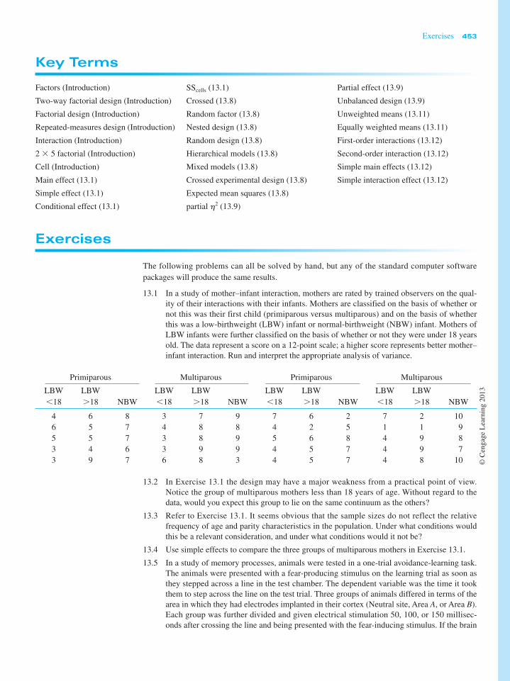
Exercises 453
Factors (Introduction)
Two-way factorial design (Introduction)
Factorial design (Introduction)
Repeated-measures design (Introduction)
Interaction (Introduction)
2 3 5 factorial (Introduction)
Cell (Introduction)
Main effect (13.1)
Simple effect (13.1)
Conditional effect (13.1)
SScells (13.1)
Crossed (13.8)
Random factor (13.8)
Nested design (13.8)
Random design (13.8)
Hierarchical models (13.8)
Mixed models (13.8)
Crossed experimental design (13.8)
Expected mean squares (13.8)
partial h2 (13.9)
Partial effect (13.9)
Unbalanced design (13.9)
Unweighted means (13.11)
Equally weighted means (13.11)
First-order interactions (13.12)
Second-order interaction (13.12)
Simple main effects (13.12)
Simple interaction effect (13.12)
Key Terms
Exercises
The following problems can all be solved by hand, but any of the standard computer software
packages will produce the same results.
13.1 In a study of mother–infant interaction, mothers are rated by trained observers on the qual-
ity of their interactions with their infants. Mothers are classified on the basis of whether or
not this was their first child (primiparous versus multiparous) and on the basis of whether
this was a low-birthweight (LBW) infant or normal-birthweight (NBW) infant. Mothers of
LBW infants were further classified on the basis of whether or not they were under 18 years
old. The data represent a score on a 12-point scale; a higher score represents better mother–
infant interaction. Run and interpret the appropriate analysis of variance.
Primiparous Multiparous Primiparous Multiparous
LBW
,18
LBW
.18 NBW
LBW
,18
LBW
.18 NBW
LBW
,18
LBW
.18 NBW
LBW
,18
LBW
.18 NBW
4 6 8 3 7 9 7 6 2 7 2 10
6 5 7 4 8 8 4 2 5 1 1 9
5 5 7 3 8 9 5 6 8 4 9 8
3 4 6 3 9 9 4 5 7 4 9 7
3 9 7 6 8 3 4 5 7 4 8 10
13.2 In Exercise 13.1 the design may have a major weakness from a practical point of view.
Notice the group of multiparous mothers less than 18 years of age. Without regard to the
data, would you expect this group to lie on the same continuum as the others?
13.3 Refer to Exercise 13.1. It seems obvious that the sample sizes do not reflect the relative
frequency of age and parity characteristics in the population. Under what conditions would
this be a relevant consideration, and under what conditions would it not be?
13.4 Use simple effects to compare the three groups of multiparous mothers in Exercise 13.1.
13.5 In a study of memory processes, animals were tested in a one-trial avoidance-learning task.
The animals were presented with a fear-producing stimulus on the learning trial as soon as
they stepped across a line in the test chamber. The dependent variable was the time it took
them to step across the line on the test trial. Three groups of animals differed in terms of the
area in which they had electrodes implanted in their cortex (Neutral site, Area A, or Area B).
Each group was further divided and given electrical stimulation 50, 100, or 150 millisec-
onds after crossing the line and being presented with the fear-inducing stimulus. If the brain
© C
engag
e L
earn
ing 2
013
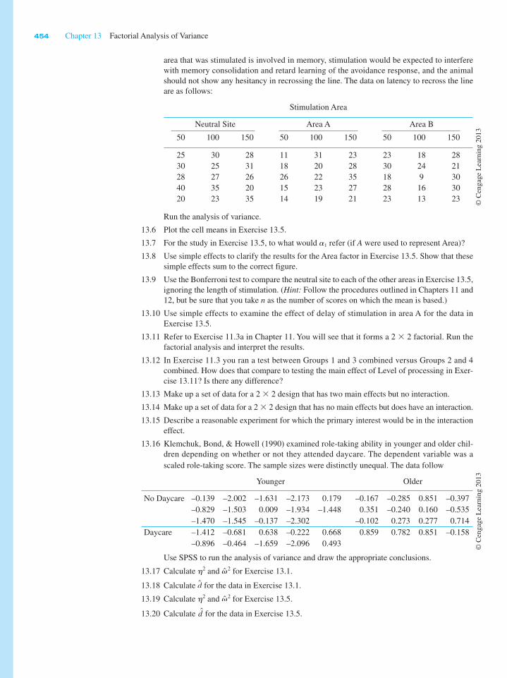
454 Chapter 13 Factorial Analysis of Variance
area that was stimulated is involved in memory, stimulation would be expected to interfere
with memory consolidation and retard learning of the avoidance response, and the animal
should not show any hesitancy in recrossing the line. The data on latency to recross the line
are as follows:
Stimulation Area
Neutral Site Area A Area B
50 100 150 50 100 150 50 100 150
25 30 28 11 31 23 23 18 28
30 25 31 18 20 28 30 24 21
28 27 26 26 22 35 18 9 30
40 35 20 15 23 27 28 16 30
20 23 35 14 19 21 23 13 23
Run the analysis of variance.
13.6 Plot the cell means in Exercise 13.5.
13.7 For the study in Exercise 13.5, to what would a1 refer (if A were used to represent Area)?
13.8 Use simple effects to clarify the results for the Area factor in Exercise 13.5. Show that these
simple effects sum to the correct figure.
13.9 Use the Bonferroni test to compare the neutral site to each of the other areas in Exercise 13.5,
ignoring the length of stimulation. (Hint: Follow the procedures outlined in Chapters 11 and
12, but be sure that you take n as the number of scores on which the mean is based.)
13.10 Use simple effects to examine the effect of delay of stimulation in area A for the data in
Exercise 13.5.
13.11 Refer to Exercise 11.3a in Chapter 11. You will see that it forms a 2 3 2 factorial. Run the
factorial analysis and interpret the results.
13.12 In Exercise 11.3 you ran a test between Groups 1 and 3 combined versus Groups 2 and 4
combined. How does that compare to testing the main effect of Level of processing in Exer-
cise 13.11? Is there any difference?
13.13 Make up a set of data for a 2 3 2 design that has two main effects but no interaction.
13.14 Make up a set of data for a 2 3 2 design that has no main effects but does have an interaction.
13.15 Describe a reasonable experiment for which the primary interest would be in the interaction
effect.
13.16 Klemchuk, Bond, & Howell (1990) examined role-taking ability in younger and older chil-
dren depending on whether or not they attended daycare. The dependent variable was a
scaled role-taking score. The sample sizes were distinctly unequal. The data follow
Younger Older
No Daycare –0.139 –2.002 –1.631 –2.173 0.179
–0.829 –1.503 0.009 –1.934 –1.448
–1.470 –1.545 –0.137 –2.302
–0.167 –0.285 0.851 –0.397
0.351 –0.240 0.160 –0.535
–0.102 0.273 0.277 0.714
Daycare –1.412 –0.681 0.638 –0.222 0.668
–0.896 –0.464 –1.659 –2.096 0.493
0.859 0.782 0.851 –0.158
Use SPSS to run the analysis of variance and draw the appropriate conclusions.
13.17 Calculate h2 and v2 for Exercise 13.1.
13.18 Calculate d for the data in Exercise 13.1.
13.19 Calculate h2 and v2 for Exercise 13.5.
13.20 Calculate d for the data in Exercise 13.5.
© C
engag
e L
earn
ing 2
013
© C
engag
e L
earn
ing 2
013
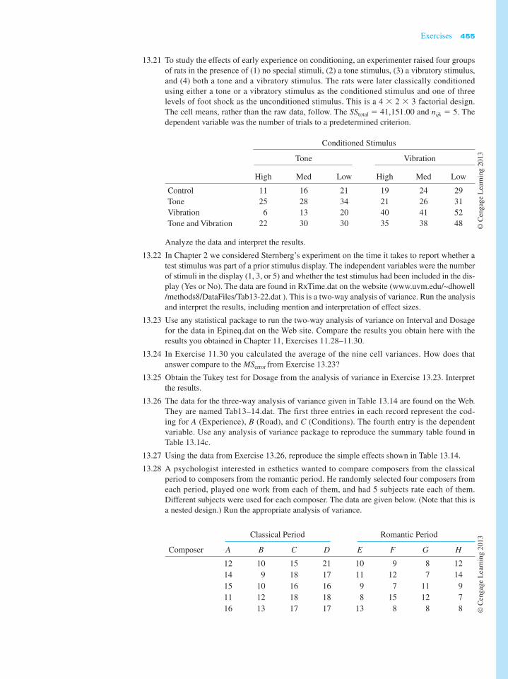
Exercises 455
13.21 To study the effects of early experience on conditioning, an experimenter raised four groups
of rats in the presence of (1) no special stimuli, (2) a tone stimulus, (3) a vibratory stimulus,
and (4) both a tone and a vibratory stimulus. The rats were later classically conditioned
using either a tone or a vibratory stimulus as the conditioned stimulus and one of three
levels of foot shock as the unconditioned stimulus. This is a 4 3 2 3 3 factorial design.
The cell means, rather than the raw data, follow. The SStotal 5 41,151.00 and nijk 5 5. The
dependent variable was the number of trials to a predetermined criterion.
Conditioned Stimulus
Tone Vibration
High Med Low High Med Low
Control 11 16 21 19 24 29
Tone 25 28 34 21 26 31
Vibration 6 13 20 40 41 52
Tone and Vibration 22 30 30 35 38 48
Analyze the data and interpret the results.
13.22 In Chapter 2 we considered Sternberg’s experiment on the time it takes to report whether a
test stimulus was part of a prior stimulus display. The independent variables were the number
of stimuli in the display (1, 3, or 5) and whether the test stimulus had been included in the dis-
play (Yes or No). The data are found in RxTime.dat on the website (www.uvm.edu/~dhowell
/methods8/DataFiles/Tab13-22.dat ). This is a two-way analysis of variance. Run the analysis
and interpret the results, including mention and interpretation of effect sizes.
13.23 Use any statistical package to run the two-way analysis of variance on Interval and Dosage
for the data in Epineq.dat on the Web site. Compare the results you obtain here with the
results you obtained in Chapter 11, Exercises 11.28–11.30.
13.24 In Exercise 11.30 you calculated the average of the nine cell variances. How does that
answer compare to the MSerror from Exercise 13.23?
13.25 Obtain the Tukey test for Dosage from the analysis of variance in Exercise 13.23. Interpret
the results.
13.26 The data for the three-way analysis of variance given in Table 13.14 are found on the Web.
They are named Tab13–14.dat. The first three entries in each record represent the cod-
ing for A (Experience), B (Road), and C (Conditions). The fourth entry is the dependent
variable. Use any analysis of variance package to reproduce the summary table found in
Table 13.14c.
13.27 Using the data from Exercise 13.26, reproduce the simple effects shown in Table 13.14.
13.28 A psychologist interested in esthetics wanted to compare composers from the classical
period to composers from the romantic period. He randomly selected four composers from
each period, played one work from each of them, and had 5 subjects rate each of them.
Different subjects were used for each composer. The data are given below. (Note that this is
a nested design.) Run the appropriate analysis of variance.
Classical Period Romantic Period
Composer A B C D E F G H
12
14
15
11
16
10
9
10
12
13
15
18
16
18
17
21
17
16
18
17
10
11
9
8
13
9
12
7
15
8
8
7
11
12
8
12
14
9
7
8
© C
engag
e L
earn
ing 2
013
© C
engag
e L
earn
ing 2
013

456 Chapter 13 Factorial Analysis of Variance
13.29 An educational researcher wanted to test the hypothesis that schools that implemented strict
dress codes produced students with higher academic performance. She randomly selected
7 schools in the state with dress codes and 7 schools that had no dress code. She then ran-
domly selected 10 students within each school and noted their performance on a standard-
ized test. The results follow.
Dress Code No Dress Code
School 1 2 3 4 5 6 7 8 9 10 11 12 13 14
91
78
86
70
78
48
89
90
85
82
75
73
65
68
70
60
72
77
75
80
80
77
70
68
70
69
64
73
70
74
84
92
78
78
77
76
74
81
75
81
59
67
68
64
75
74
67
56
61
67
62
93
83
78
65
71
65
85
74
83
87
78
83
79
53
66
76
67
74
72
69
74
67
64
61
76
74
71
62
67
72
56
71
92
88
64
79
73
72
70
78
77
75
56
84
83
67
70
31
70
66
55
58
73
55
70
64
52
64
79
67
82
76
78
87
87
63
68
86
84
52
71
73
68
65
69
79
67
66
64
63
65
75
82
77
81
67
73
72
56
13.30 Rerun the analysis in Exercise 13.29 but treat both variables as fixed and crossed. Show that
the SSschool(code) in Ex13-31 is the sum of SSschool and SSschool*code in this analysis. (Hint: If you run this using SPSS you will have to have both sets of schools numbered 1–7.)
13.31 Gartlett & Bos (2010) presented data on the outcomes of male and female children raised by
same-sex (lesbian) parents and those raised by opposite-sex parents. In a longitudinal study
following 78 children of same-sex parents for 17 years, she collected data on Achenbach’s
Child Behavior Checklist when the children were 17. She used an equal sample of raw data
from normative data collected by Achenbach on a random sample of children. For conven-
ience we will assume that each cell contained 43 children. The data are shown below.
GroupSame-Sex
Males
Same-Sex
Females
Opposite-Sex
Males
Opposite-Sex
Females
Mean
sdn
25.8
3.6
43
26.3
5.0
43
23.0
4.0
43
20.3
4.5
43
Compute an analysis of variance on these data and interpret the results. (Higher scores
reflect greater competence.) (The F values differ somewhat from hers because she analyzed
the data with a multivariate analysis of variance, but the means agree with hers. An SPSS
version of data with these means and variances is available on the Web as Ex13-31.sav.)
Discussion Questions
13.32 In the analysis of Seligman et al. (1990) data on explanatory style (Table 13.15), you will
note that there are somewhat more males than females in the Optimist group and more
females than males in the Pessimist group. Under what conditions might this affect the way
you would want to deal with unequal sample sizes, and when might you wish to ignore it?
13.33 Find an example of a three-way factorial in the research literature in which at least one
of the interactions is significant and meaningful. Then create a data set that mirrors those
results.
© C
engag
e L
earn
ing 2
013
© Cengage Learning 2013
Related Documents