1200 years of warm-season temperature variability in central Fennoscandia inferred from tree-ring density

CPD11, 489–519, 2015

1200 years ofwarm-seasontemperature

variability

P. Zhang et al.

Title Page

Abstract Introduction

Conclusions References

Tables Figures

J I

J I

Back Close

Full Screen / Esc

Printer-friendly Version

Interactive Discussion

Discussion

Paper

|D

iscussionP

aper|

Discussion

Paper

|D

iscussionP

aper|

Clim. Past Discuss., 11, 489–519, 2015www.clim-past-discuss.net/11/489/2015/doi:10.5194/cpd-11-489-2015© Author(s) 2015. CC Attribution 3.0 License.

This discussion paper is/has been under review for the journal Climate of the Past (CP).Please refer to the corresponding final paper in CP if available.

1200 years of warm-season temperaturevariability in central Fennoscandiainferred from tree-ring density

P. Zhang1, H. W. Linderholm1, B. E. Gunnarson2, J. Björklund3, and D. Chen1

1Regional Climate Group, Department of Earth Sciences, University of Gothenburg,Gothenburg, Sweden2Bert Bolin Centre for Climate Research, Department of Physical Geography and QuaternaryGeology, Stockholm University, Stockholm, Sweden3Swiss Federal Research Institute WSL, Birmensdorf, Switzerland

Received: 12 January 2015 – Accepted: 27 January 2015 – Published: 19 February 2015

Correspondence to: P. Zhang ([email protected])

Published by Copernicus Publications on behalf of the European Geosciences Union.

489

http://www.clim-past-discuss.net

http://www.clim-past-discuss.net/11/489/2015/cpd-11-489-2015-print.pdf

http://www.clim-past-discuss.net/11/489/2015/cpd-11-489-2015-discussion.html

http://creativecommons.org/licenses/by/3.0/

CPD11, 489–519, 2015


variability

P. Zhang et al.

Title Page



Tables Figures

J I

J I

Back Close

Full Screen / Esc



Discussion

Paper

|D

iscussionP

aper|

Discussion

Paper

|D

iscussionP

aper|

Abstract

An improved and extended Pinus sylvestris L. (Scots Pine) tree-ring maximum density(MXD) chronology from the central Scandinavian Mountains was used to reconstructwarm-season (April–September) temperature back to 850 CE. Due to systematic biasfrom differences in elevation (or local environment) of the samples through time, the5

data was “mean adjusted’. The new reconstruction, called C-Scan, was based onthe RSFi standardisation method to preserve mid- and long-term climate variability.C-Scan, explaining more than 50 % of the warm-season temperature variance in alarge area of Central Fennoscandia, agrees with the general profile of Northern Hemi-sphere temperature evolution during the last 12 centuries, supporting the occurrences10

of a Medieval Climate Anomaly (MCA) around 1009–1108 CE and a Little Ice Age (LIA)ca 1550–1900 CE in Central Fennoscandia. C-scan suggests a later onset of LIA anda larger cooling trend during 1000–1900 CE than previous MXD based reconstructionsfrom Northern Fennoscandia. Moreover, during the last 1200 years, the coldest periodwas found in the late 17th–19th centuries with the coldest decades being centered on15

1600 CE, and the warmest 100 years occurring in the most recent century.

1 Introduction

Fennoscandia has a strong tradition in dendrochronology, and its large tracts of bo-real forest make the region well suited for the development of tree-ring chronologiesthat extend back several thousands of years (Linderholm et al., 2010). In addition to20

the well-known multi-millennial tree-ring width chronologies from Torneträsk (Gruddet al., 2002), Finnish Lapland (Helama et al., 2002) and Jämtland (Gunnarson et al.,2003), several millennium long temperature-sensitive tree-ring datasets were collectedwithin the European Union funded “Millennium” project (McCarroll et al., 2013). How-ever, these are all, except for Jämtland and Mora (822 year Blue intensity, Graham25

et al., 2011), located in northernmost Fennoscandia. It has been shown that in or-

490





CPD11, 489–519, 2015


variability

P. Zhang et al.

Title Page



Tables Figures

J I

J I

Back Close

Full Screen / Esc



Discussion

Paper

|D

iscussionP

aper|

Discussion

Paper

|D

iscussionP

aper|

der to better represent Fennoscandian warm-season temperature variability, data frommore southern locations are needed (Linderholm et al., 2014a). Thus, getting high-quality data from the central parts of Fennoscandia is needed. Helama et al. (2014)reconstructed May–September temperature variability in southern Finland for the lastmillennium using maximum latewood density (MXD) data. In Sweden, presently the5

southernmost site to provide a robust temperature signal from tree-ring MXD data isthe central Scandinavian Mountains, in the province of Jämtland, where Gunnarsonet al. (2011, henceforth G11) reconstructed 900 years of warm-season temperatures.Because of the relatively southerly location, Jämtland is considered a key location forpaleotemperature studies in Scandinavia. Not only can it function as a link between10

chronologies in northern Fennoscandia and those in continental Europe (Gunnarsonet al., 2011), but also the closeness to the North Atlantic makes it a suitable placeto investigate long-term associations between marine and terrestrial climate variability(e.g., Cunningham et al., 2013).

At northern high latitudes, MXD and the newly developed ∆Density parameter are15

the most powerful warm-season temperature tree-ring proxies, compared to tree-ringwidths (Briffa et al., 2002; Björklund et al., 2014). The longest MXD records are foundin northernmost Fennoscandia (see McCarroll et al., 2013; Melvin et al., 2013; Es-per et al., 2012). These chronologies are exclusively based on material with knowntemperature sensitive provenience, from living trees, dry deadwood and, in the case of20

N-Scan, subfossil wood (Esper et al., 2012). The G11, however, also included historicalmaterial (tree-ring samples from historical buildings). The historical samples were col-lected from buildings in Jämtland in the 1980s, as a part of a grand sampling strategyto focus on a dense tree-ring density network from cool moist regions (Schweingruberet al., 1990). Due to the limited number of deadwood samples from the studied area in25

the Scandinavian Mountains, the historical samples, belonging to the period between1107 and 1827 CE (with a gap between 1292–1315 CE), made up the major part of theG11 reconstruction. Since the geographical origin of the historical samples is unclear,it was difficult to fully assess the validity of the interpreted temperature signal. Compar-

491





CPD11, 489–519, 2015


variability

P. Zhang et al.

Title Page



Tables Figures

J I

J I

Back Close

Full Screen / Esc



Discussion

Paper

|D

iscussionP

aper|

Discussion

Paper

|D

iscussionP

aper|

ing G11 to the Fennoscandian June–August summer temperature reconstruction fromGouirand et al. (2008), a coherency was found between AD 1300 and 1900, but G11showed a stronger warming between AD 1100 and 1300. One explanation for the differ-ences between the two records could be regional differences in the temporal evolutionof warm-season temperatures in central and northern Scandinavia (Gunnarson et al.,5

2011). For instance, Gunnarson and Linderholm (2002) suggested that the MedievalClimate Anomaly (MCA, 10th–13th CE, Grove and Switsur, 1994) was of shorter dura-tion but more pronounced in the central Scandinavian Mountains compared to North-ern Scandinavia. Another reason for this apparent difference in late-MCA temperaturescould be that the tree-ring samples collected from the historical buildings do not truly10

reflect summer temperature variability in the mountains due to their likely low-elevationorigins.

To overcome this uncertainty, we developed a warm-season (April through Septem-ber) temperature reconstruction for the last 1200 years based exclusively on Scots pinesamples from sites close to the current altitude timber-line in a relatively limited area.15

Since there was an elevational difference in the temporal distribution of the samples,we also considered the impact of the temperature lapse rate and local environment onMXD values, and corrected the MXD values according to the mean-adjustment method(Zhang et al., 2015). Furthermore, the traditional RCS (regional curve standardisation)method (Briffa et al., 1992) was compared with the new RSFi (regional curve adjusted20

individual signal-free approach) method (Björklund et al., 2014) when developing thechronology.

2 Data and method

2.1 Study area

The province of Jämtland is located in the westernmost part of central Sweden (Fig. 1).25

The region belongs to the Northern Boreal zone, and the study area is situated just

492





CPD11, 489–519, 2015


variability

P. Zhang et al.

Title Page



Tables Figures

J I

J I

Back Close

Full Screen / Esc



Discussion

Paper

|D

iscussionP

aper|

Discussion

Paper

|D

iscussionP

aper|

east of the Scandinavian Mountains main divide. The main topography ranges from800 to 1000 ma.s.l., but scattered alpine massifs to the south reach approximately1700 ma.s.l. There is a distinct climate gradient in the area. East of the ScandinavianMountains, climate can be described as semi-continental. However, the proximity tothe Norwegian Sea, lack of high mountains in the west, and the east–west oriented5

valleys allow moist air to be advected from the ocean, providing an oceanic influenceto the area. Consequently, the study area is located in a border zone between oceanicand continental climates. On short timescales, summer climate of this particular re-gion is influenced by the atmospheric circulation, mainly the North Atlantic Oscillation(NAO) (Chen and Hellström, 1999), while it is affected by North Atlantic sea-surface10

temperature (SST) on longer timescales (Rodwell et al., 1999; Rodwell and Folland,2002).

Glacial deposits dominate the area, mainly till but also glacifluvial deposits, peatlandsand small areas of lacustrine sediments (Lundqvist, 1969). The forested parts in thecentral Scandinavian Mountains are dominated by Pinus sylvestris L. (Scots Pine),15

Picea abies (Norway spruce) and Betula pubescens (Mountain birch). Although large-scale forestry have been carried out in most parts of the county, the human impacton trees growing close to the tree line is limited, which is valuable in tree-ring basedclimate reconstructions (Gunnarson et al., 2012). Due to the short and cool summers,dry deadwood can be preserved for more than 1000 years (Linderholm et al., 2014b).20

Moreover, large amounts of subfossil wood from hundreds to thousands of years agocan be found in small mountain lakes (see Gunnarson, 2008).

2.2 Tree-ring data

The tree-ring data used in this study came from 8 sites (Table 1). As shown inFig. 1, they are all at a close distance, but differ in elevation and local environ-25

ment. From the small peak Furuberget, 142 samples were collected close to thetop at ca. 650 ma.s.l. in an open pine forest with limited competition between trees.Pine trees grow on a relatively flat area covered by a thick vegetation layer with

493





CPD11, 489–519, 2015


variability

P. Zhang et al.

Title Page



Tables Figures

J I

J I

Back Close

Full Screen / Esc



Discussion

Paper

|D

iscussionP

aper|

Discussion

Paper

|D

iscussionP

aper|

woody dwarf shrubs and mosses. The area is characterized by thin till and glaciflu-vial soils. 35 of these samples were included in G11 (Table 1). In addition, pine sam-ples were collected at different elevations on Mount Håckervalen from the presenttree line (at around 650 ma.s.l.) up to 800 ma.s.l., described in detail in Linderholmet al. (2014b). At both sites living trees and dry deadwood were sampled. Sam-5

ples preserved in lakes (so called subfossil wood) were included from the lakes Lill-Rörtjärnen, Östra Helgtjärnen and Jens-Perstjärnen, previously described in Gun-narson (2008). The historical tree-ring data, collected from historical buildings in theprovince was downloaded from the International Tree-Ring Data Bank (ONLINE RE-SOURCE: https://www.ncdc.noaa.gov/paleo/study/4447).10

The new MXD measurements (Table 1) were produced using an ITRAX Wood scan-ner from Cox Analytic System (http://www.coxsys.se). For further information of theITRAX settings, see Gunnarson et al. (2011). The historical samples was collected bySchweingruber et al. in the 1970s (Schweingruber et al., 1991) and the MXD mea-surements was obtained using the DENDRO2003 x-ray instrumentation from Walesh15

Electronic (http://www.walesch.ch/). All samples were prepared according to standarddendrochronological techniques (Schweingruber et al., 1978).

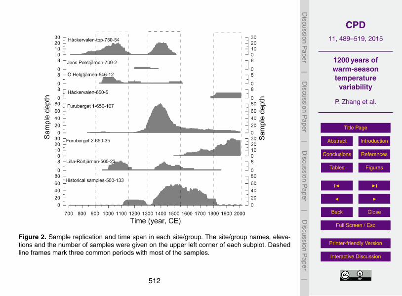
It was previously found that in the studied region, the absolute MXD values differwith respect to elevation, which is likely due to the temperature lapse rate (Zhanget al., 2015). In short, the absolute MXD values at higher elevation are systematically20

lower than those from lower elevation. Moreover, the elevation effect on the absoluteMXD values is larger than the effect of temperature differences between warm (MCA)and cold (Little Ice Age, LIA, 14th–19th centuries Grove, 2001) periods. Thus, an aver-age chronology with a heterogeneous elevational sample distribution through time, e.g.older samples are found only at progressively higher elevations, will contain systematic25

differences in their means during different periods. If not attended to this may introducebiases to an average chronology, both in terms of the high-resolution variability (annualto decadal) and the long term trend. It is evident from Fig. 2, that there are periodswhen the samples from different elevations do not overlap in time, e.g. 1550–1800 (no

494





https://www.ncdc.noaa.gov/paleo/study/4447

http://www.coxsys.se

http://www.walesch.ch/

CPD11, 489–519, 2015


variability

P. Zhang et al.

Title Page



Tables Figures

J I

J I

Back Close

Full Screen / Esc



Discussion

Paper

|D

iscussionP

aper|

Discussion

Paper

|D

iscussionP

aper|

samples from Håckervalen-top and Furuberget 1 overlap.). To overcome this problem,we adjusted the mean MXD value from the different elevations to have the same meanduring a period of overlap. The mean MXD value of the Furuberget 1 samples, cov-ering 1300–1550, was used as a reference to adjust the samples from other groupsexcept for the sites Håckervalen and Furuberget 2 (samples from these two groups5

do not cover 1300–1550). A constant was added to or subtracted from each sampleof a group in order to force the samples to have the same mean MXD value as thereference. Since the living trees from Håckervalen (650 m) and Furuberget 2 have thesame elevation as Furuberget 1, and both of the sites do not have significantly differentmean MXD values with the Furuberget 1 samples during 1800–2000, we did not adjust10

the samples from these two sites. We chose Furuberget 1 as a reference site, becausethe Furuberget 1 samples had a high sample replication and a wide temporal cover-age. Other ways to deal with this problem is to standardise the samples site-by-site(or group-by-group) rather than adjusting the mean value of each group of samples.However, this method works well when all groups have the same or similar temporal15

distribution.

2.3 Standardisation method and chronology building

If tree-ring data is going to be used to attain reliable climate information, it is pertinentto remove as much non-climatic information as possible before building a chronologyfrom the individual tree-ring series (Fritts, 1976). The non-climatological growth ex-20

pression is usually represented with a least square fitted negative exponential function,polynomial or spline (Fritts, 1976; Cook and Peters, 1981), and subtracted or dividedfrom each raw tree-ring measurement to obtain indices used for chronology building, ina process termed standardisation. This approach is widely used, but it severely limitsthe attained low-frequency variability in long chronologies (with several generations of25

trees), because all indices have similar averages, referred to as the “segment lengthcurse” (Cook et al., 1995; Briffa et al., 1996).

495





CPD11, 489–519, 2015


variability

P. Zhang et al.

Title Page



Tables Figures

J I

J I

Back Close

Full Screen / Esc



Discussion

Paper

|D

iscussionP

aper|

Discussion

Paper

|D

iscussionP

aper|

This limitation can be overcome by quantifying the non-climatological growth ex-pression for an entire population as an average of the growth of all samples aligned bycambial age, which then can be represented by a single mathematical function. Subse-quently this function is subtracted from or divided by each individual tree-ring measure-ment, where this process is called Regional Curve Standardisation (RCS Briffa et al.,5

1992). However, by using one single function for all tree-ring series, less unwantedmid-frequency variability is removed in the attempt to preserve the low-frequency(> segment length) variability (Melvin, 2004), along with possible trend distortion asdescribed in Melvin and Briffa (2008). Alternatively, the non-climatological expressionin tree-ring data can be quantified with the signal-free (SF) approach to standardisa-10

tion, described in Melvin and Briffa (2008), either on individual trees or on an averageof all trees (RCS). Using SF RCS can alleviate possible trend distortions, but limitednoise from stand competition etc. is removed.

By using the SF individual fitting approach and at the same time letting the de-rived functions to have a similar mean as their respective cambial age segment of15

the regional curve (RC) before subtraction into indices, stand competition etc. can alsobe addressed without losing the long timescale component (Björklund et al., 2013).This approach was termed RSFi (ibid.). We compared chronologies resulting from theabove described standardisation methods: classic RCS, SF RCS and RSFi, where thechronology used for reconstruction was derived with RSFi. The expressed population20

signal (EPS) criterion was used to evaluate the robustness of the chronology. An EPSvalue represents the percentage of the variance in the hypothetical population signalin the region that is accounted for by the chronology, where EPS values greater than0.85 are generally regarded as sufficient (Wigley et al., 1984).

2.4 Instrumental data25

Monthly temperature data from the closest meteorological station, Duved (400 ma.s.l.,63.38◦N, 12.93◦ E), was used to assess the temperature signal reflected by thechronology. Since the data from this station only cover the period of 1911–1979,

496





CPD11, 489–519, 2015


variability

P. Zhang et al.

Title Page



Tables Figures

J I

J I

Back Close

Full Screen / Esc



Discussion

Paper

|D

iscussionP

aper|

Discussion

Paper

|D

iscussionP

aper|

we extended the data back to 1890 and up to 2011 by using linear regression onmonthly temperature data from an adjacent station: Östersund (376 ma.s.l., 63.20◦N,14.49◦ E). A linear regression was done to relate mean temperature of each monthfrom Östersund station to that from Duved station. Data from Östersund explain on av-erage 91.5 % of the interannual variance in Duved monthly temperature (based on the5

overlapping period 1911–1979). The temperature data from Östersund came from twosources: the Nordklim data base (1890–2001) (Tuomenvirta et al., 2001), and SwedishMeteorological and Hydrological Institute (SMHI, 2001–2011). The locations of Duvedand Östersund stations are shown in Fig. 1.

3 Warm-season temperatures reconstruction10

3.1 Comparing MXD samples of different origin

After having adjusted the mean value of each group of samples, we compared the twochronologies based on the “in situ” and historical samples respectively. Three stan-dardisation methods were applied to build the chronologies. Figure 3 shows a compar-ison of the z scored (based on 1700–1800) historical-sample chronology (HSC, blue15

curves) and the ”in situ”- chronology (ISC, black curves) produced by the signal-freeRCS (Fig. 3a), negative exponential function standardisation (Fig. 3b), and RSFi stan-dardisation (Fig. 3c) methods. Clearly, the same features can be observed regardlessof the standardisation methods: (1) on multidecadal scales, the HSC agrees quite wellwith ISC between 1300 and 1800 CE, but the HSC displays a smaller variance than20

the ISC; (2) between 1100 and 1300 CE there is a notable disagreement between HSCand ISC. On interannual scale (based on 1st difference chronologies), the HSC canexplain 34 % variance of ISC during 1100–1300 CE, and explain 62 % of the varianceduring 1300–1800 CE. Moreover, it should be noted that the 50 year-window EPS val-ues fall below 0.85 for both chronologies during the 1160–1220 CE period. We tested25

boosting the ISC with the historical samples during 1100–1300. The statistic results

497





CPD11, 489–519, 2015


variability

P. Zhang et al.

Title Page



Tables Figures

J I

J I

Back Close

Full Screen / Esc



Discussion

Paper

|D

iscussionP

aper|

Discussion

Paper

|D

iscussionP

aper|

show that the EPS of the boosted chronology during 1160–1210 is still below 0.85, andthe EPS during 1225–1265 is even smaller than before boosting. Only the EPS during1212–1222 changed from below 0.85 to above 0.85. Consequently, there was no sig-nificant improvement of the robustness of the ISC during 1100–1300 CE after includingthe historical samples.5

3.2 The influence of standardisation method

At present, RCS and signal-free RCS are the most favoured standardisation methodswhen building chronologies intended to have their long-term variability preserved. Weexamined the performances of the two RCS methods and the RSFi method. As shownin Fig. 4, the difference among the three differently standardised chronologies is mainly10

reflected in the multi-decadal variability. The chronologies produced by the both RCSmethods are in very good agreement on multi-decadal timescales. Although the RSFichronology shows a similar evolution as the RCS ones, it is obvious that they differin some periods. In general, the RSFi chronology suggests slightly warmer conditionsthan the RCS based ones, especially pronounced during the late half of LIA. It is diffi-15

cult to firmly state which one of the chronologies is closer to actual temperatures, butwe argue that there is a benefit in using individual signal-free curves (the RSFi method)rather than a common regional signal-free curve (the RCS methods), since this proce-dure has a better potential to remove unwanted noise (e.g. related to stand dynamics)on tree level. Consequently, we opted for the RSFi chronology for the reconstruction.20

3.3 Climate signal in the new chronology

We compared the new chronology with the instrumental monthly mean temperaturesconstructed for the Duved meteorological station during the period 1890–2011. Fig-ure 5a shows that the new chronology has a significant positive correlation (at p < 0.01level) with individual monthly mean temperatures in April through September, and25

the highest correlation was found with mean April–September temperature (r = 0.77).

498





CPD11, 489–519, 2015


variability

P. Zhang et al.

Title Page



Tables Figures

J I

J I

Back Close

Full Screen / Esc



Discussion

Paper

|D

iscussionP

aper|

Discussion

Paper

|D

iscussionP

aper|

Therefore, we decided to reconstruct the April–September mean temperature (hence-forth referred to as warm-season temperature). The reconstructed and observed warm-season temperatures for the 1890–2011 period show a good agreement on interanualto multidecadal timescales (Fig. 5c), and the new MXD reconstruction explains approx-imately 59 % of the variance in the instrumental data (Fig. 5b).5

3.4 The new reconstruction

In order to test the temporal stability of the MXD vs. observation when creating a modelto reconstruct warm-season temperature back in time, we divided the instrumental pe-riod into two parts: 1890–1950 and 1951–2011, with the first part for calibration and thesecond part for verification. Then, we switched the calibration and verification periods,10

and repeated the same exercise. The calibration and verification statistics are shown inTable 2. The reduction of error statistic (RE) has a possible range of −∞ to 1, and anRE of 1 can be achieved only if the prediction residuals equal zero. Zero is commonlyused as a threshold, and the positive RE values in the both calibration periods suggeststhat our reconstruction has some skill (Table 2). Similar to RE, coefficient of efficiency15

(CE) is a measure to evaluate the model under the validation period. Values close tozero or negative suggests that the reconstruction is no better than the mean, whereaspositive values indicate the strength and temporal stability of the reconstruction.

We evaluated the spatial representativeness of the new warm-season temperaturereconstruction by correlating it with the CRU TS3.22 0.5◦ ×0.5◦ gridded warm-season20

temperature (Harris et al., 2014) for the period 1901–2011. The field correlation mapswere plotted using the “KNMI climate explorer” (Royal Netherlands meteorological In-stitute; http://climexp.knmi.nl; Van Oldenborgh et al., 2009). We also compared the fieldcorrelation of observed warm-season temperature. As expected, Fig. 6 shows that thenew reconstruction (Fig. 6a) captures a large part of the patterns from the observa-25

tions (Fig. 6b). The reconstruction represents the warm-season temperature variationwith correlations above 0.71 across much of Central Fennoscandia, which validatesthe good spatial representativeness of our reconstruction.

499





http://climexp.knmi.nl

CPD11, 489–519, 2015


variability

P. Zhang et al.

Title Page



Tables Figures

J I

J I

Back Close

Full Screen / Esc



Discussion

Paper

|D

iscussionP

aper|

Discussion

Paper

|D

iscussionP

aper|

4 Discussion

4.1 Central Fennoscandian warm-season temperature evolution

Figure 7 shows the reconstructed warm-season temperature of Central Fennoscan-dian, henceforth C-Scan, during the past 1200 years. C-Scan displays a cooling trendbetween 850 and 1800 CE, followed by a sharp temperature increase after the mid-5

19th century. In order to look at the C-Scan temperature evolution in more detail, wepicked out the coldest and warmest periods (10, 30 and 100 years of mean tempera-tures respectively) during the last 1200 years (Fig. 7). The late 17th century to early19th century was the coldest long-term period during the past 1200 years, and thatthe coldest 100 year-period appeared during the 19th century. Both the coldest 10 and10

30 year periods appeared during the 17th century. The warmest 100 years coincideswith the most recent 100 years, which is consistent with the anthropogenic warmingperiod (Stocker et al., 2013). However, the warmest 10 and 30 year periods were foundin the 13th century. Comparing the MCA with the current warming period showed thatthe warmest 100 year period during the MCA was 0.1 ◦C cooler than the 20th cen-15

tury. The warmest 10 and 30 year periods during the 20th century were 0.2 and 0.1 ◦Ccooler respectively than those during the 13th century. Despite low sample depth, thewarmest 10 and 30 year periods have 51 year EPS values above 0.85.

4.2 The influence on MXD of elevation differences

To highlight the application of mean-adjusted data in our reconstruction, we compared20

reconstructions based on mean-adjusted and unadjusted samples. As shown in Fig. 8,the reconstruction based on unadjusted samples (blue curve) yields a 0.4 ◦C loweraverage warm-season temperature during the period 850–1200 CE compared to themean-adjusted reconstruction (black curve). Moreover, the long-term trend before theonset of the twentieth century clearly differs between the two, where the cooling trend in25

the mean-adjusted data is turned to a warming trend in the unadjusted. Consequently,

500





CPD11, 489–519, 2015


variability

P. Zhang et al.

Title Page



Tables Figures

J I

J I

Back Close

Full Screen / Esc



Discussion

Paper

|D

iscussionP

aper|

Discussion

Paper

|D

iscussionP

aper|

a reconstruction based on unadjusted data would indicate that warm-season tempera-ture in 850–1200 CE, roughly corresponding to the MCA, would be about 0.3 ◦C coolerthan the subsequent four centuries (1201–1600 CE). This is quite contradictory to in-dications from other paleoclimate data for Fennoscandia (e.g., Esper et al., 2012; Mc-Carroll et al., 2013; Melvin et al., 2013; Helama et al., 2014), as well as for the whole5

Northern Hemisphere.Previous ways of dealing with samples of different origin (living trees, subfossil and

historical wood), have used separate RCS curves for each type of samples (e.g., Gun-narson et al., 2011), but the prerequisite is that samples of different origin are fromthe same periods, or at least have a large overlap, so that any differences in long-term10

trend are to a large extent cancelled out when averaging. Given that we did have someoverlap between our different data, we could have used the “separate RCS curves”method. However, although this method produces a similar reconstruction after themid-13th century, it does deliver a mean temperature for 850–900 and 1150–1250 CEthat is 0.2 ◦C lower than that by our method. Therefore, we choose to use of the mean-15

adjustment method.

4.3 Comparing C-Scan with Northern Hemisphere temperature pattern andNorthern Fennoscandia MXD reconstruction

To set our new reconstruction in a wider context, we compared it with the North-ern Hemisphere temperature patterns based on multi-proxy records (Ljungqvist et al.,20

2012). Our new reconstruction shows an agreement with the general profile of NorthernHemisphere temperature evolution during the last 12 centuries, supporting the occur-rences of a MCA and LIA in Central Fennoscandia. The hemisphere scale temperaturepatterns shows that, despite differences in the onset of MCA or LIA phases regionally,the Northern Hemisphere generally experience a relative warm period during 800–25

1300 CE and a relative cold period during 1300–1900 CE, and followed by an intensivewarming period after 1900 CE. However, there are some aspects where our recon-struction shows differences. One such aspect is that the warmest century during MCA

501





CPD11, 489–519, 2015


variability

P. Zhang et al.

Title Page



Tables Figures

J I

J I

Back Close

Full Screen / Esc



Discussion

Paper

|D

iscussionP

aper|

Discussion

Paper

|D

iscussionP

aper|

in our reconstruction occurred during the 11th century, while the Northern Hemispheretemperature peak is found in the 10th century. Another aspect is that the cooling fromMCA to the LIA seems to happen at a stable rate on the hemisphere scale, whileour reconstruction shows a weak cooling during the transition period from the MCAto the LIA (1300–1500 CE), followed by an intensive cooling during the 16th century5

when central Scandinavia enter into a 300 year cold period. Globally, continental-scaletemperature has shown a regional difference in temporal evolution during the last twomillennia under natural forcings conditions (Ahmed et al., 2013). Thus, the lag of thewarmest century during MCA and the late onset of LIA in central Fennoscandia can beexplained by the regional temperature evolution. However, considering the late onset10

of LIA, our reconstruction seems more similar with the temperature evolution in NorthAmerica and Australia rather than Arctic, Europe and Asia.

Zooming in to Fennoscandia, we compared C-Scan to the MXD derived summertemperature reconstruction from northern Fennoscandia (N-Scan, Esper et al., 2012).From Fig. 10a, it is clear that although our new reconstruction agrees well with the15

long-term cooling up until 1900, discussed by Esper et al. (2012), some obvious differ-ences can be noted. The long term cooling trend is slightly more pronounced in C-Scan(0.48 ◦C per 1000 years over the period of 1000–1900 CE, compared to 0.36 ◦C in N-Scan). Moreover, C-Scan infers cooler temperatures than N-Scan during two longerperiods roughly corresponding to the early half of MCA (900–1100 CE) and late half of20

LIA (1550–1900 CE). Also, the two records seem to be offset between 850 and 1300.However, it should be noted that the two reconstructions agree quite well on interannualtimescale, except for the period 1230–1280. The more or less anti-phase behaviour inC-Scan between 1150 and 1250 is likely due to the drop in sample sizes in C-Scanat that time. Comparing the 101 year running R-bar in the two MXD series (after age-25

dependent spline detrending) of the two reconstructions shows that the mean runningR-bar values are 0.45 and 0.46 for C-Scan (65 series (trees) covering 850–1406 CE)and N-Scan samples (50 series (trees) covering 850–1404 CE) respectively. This in-

502





CPD11, 489–519, 2015


variability

P. Zhang et al.

Title Page



Tables Figures

J I

J I

Back Close

Full Screen / Esc



Discussion

Paper

|D

iscussionP

aper|

Discussion

Paper

|D

iscussionP

aper|

dicates that both reconstructions reflect common signals of their respective samplepopulations during the period of disagreement.

When compared with the 1500 year long MXD based May–August temperature re-construction from Torneträsk (Melvin et al., 2013), C-Scan infers slightly warmer tem-peratures during 1200–1700 CE, and in general differs from the Torneträsk reconstruc-5

tion at multi-decadal to century timescales during 1100–1900 CE. However, they are inquite good agreement on interannual timescale. The running R-bar curves also indicatethe both reconstructions reflect common signals of their respective sample population.

Despite the proximity, C-scan shows some different features from the temperatureevolution in Northern Fennoscandia, such as a later onset of the LIA. This possibly10

indicates that the warm-season temperature evolution differs also within Fennoscan-dia. Under anthropogenic forcing conditions, global temperature shows a significantwarming trend. However, the warming trends can be different in their magnitudes indifferent regions, due to differnces in regional settings and processes. In addition tothe different heat capacity between continent and ocean and the snow-ice feedback,15

other physical mechanisms behind this should be well addressed in order to project thefuture regional temperature. To well address this issue, more high resolution regionaltemperature reconstructions are needed.

5 Conclusions

An updated and extended version of the Jämtland MXD chronology was used to20

reconstruct the warm-season temperature (April–September) evolution in CentralFennoscandia for the period 850–2011 CE. Due to the fact that the samples comefrom different elevations, the new reconstruction, called C-Scan, was based on mean-adjusted data subsequently standardised with the RSFi method. Our new reconstruc-tion suggests a MCA during ca 1009 to 1108, followed by a transition period be-25

fore the onset of the Little Ice Age proper in the mid-16th century. The cooling trend(−0.48 ◦C per 1000 years) during 1000–1900 is greater than that inferred from northern

503





CPD11, 489–519, 2015


variability

P. Zhang et al.

Title Page



Tables Figures

J I

J I

Back Close

Full Screen / Esc



Discussion

Paper

|D

iscussionP

aper|

Discussion

Paper

|D

iscussionP

aper|

Fennoscandia (Esper et al., 2012). During the last 1200 years, the late 17th century toearly 19th century was the coldest period in central Fennoscandia, and the warmest100 years occurred during the most recent century in central Fennoscandia, and thecoldest decades occurred around 1600 CE.

Acknowledgements. We acknowledge the County Administrative Boards of Jämtland for giving5

permissions to conduct dendrochronological sampling, and Mauricio Fuentes, Petter Stridbeck,Riikka Salo, Emad Farahat and Eva Rocha for their help in the field. We also thank Laura McG-lynn and Håkan Grudd for assistance in the MXD measurements and Andrea Seim for helpingout with GIS. This work was supported by Grants from the two Swedish research councils(Vetenskapsrådet and Formas, Grants to Hans Linderholm) and the Royal Swedish Academy10

of Sciences (Kungl. Vetenskapsakademien, grant to Peng Zhang). This research contributes tothe strategic research areas Modelling the Regional and Global Earth system (MERGE), andBiodiversity and Ecosystem services in a Changing Climate (BECC) and to the PAGES2K initia-tive. This is contribution # 33 from the Sino-Swedish Centre for Tree-Ring Research (SISTRR).

References15

Ahmed, M., Anchukaitis, K., Buckley, B. M., Braida, M., Borgaonkar, H. P., Asrat, A., Cook, E. R.,Büntgen, U., Chase, B. M., and Christie, D. A.: PAGE 2k Consortium: Continental-scale tem-perature variability during the past two millennia, Nat. Geosci., 6, 339–346, 2013. 502

Björklund, J. A., Gunnarson, B. E., Krusic, P. J., Grudd, H., Josefsson, T., Östlund, L., and Lin-derholm, H. W.: Advances towards improved low-frequency tree-ring reconstructions, using20

an updated Pinus sylvestris L. MXD network from the Scandinavian Mountains, Theor. Appl.Climatol., 113, 697–710, 2013. 496

Björklund, J. A., Gunnarson, B. E., Seftigen, K., Esper, J., and Linderholm, H. W.: Blue inten-sity and density from northern Fennoscandian tree rings, exploring the potential to improvesummer temperature reconstructions with earlywood information, Clim. Past, 10, 877–885,25

doi:10.5194/cp-10-877-2014, 2014. 491, 492Briffa, K. R., Jones, P. D., Bartholin, T. S., Eckstein, D., Schweingruber, F. H., Karlen, W., Zetter-

berg, P., and Eronen, M.: Fennoscandian summers from AD 500: temperature changes onshort and long timescales, Clim. Dynam., 7, 111–119, 1992. 492, 496

504





http://dx.doi.org/10.5194/cp-10-877-2014

CPD11, 489–519, 2015


variability

P. Zhang et al.

Title Page



Tables Figures

J I

J I

Back Close

Full Screen / Esc



Discussion

Paper

|D

iscussionP

aper|

Discussion

Paper

|D

iscussionP

aper|

Briffa, K. R., Jones, P. D., Schweingruber, F. H., Karlén, W., and Shiyatov, S. G.: Tree-RingVariables as Proxy-Climate Indicators: Problems with Low-Frequency Signals, Springer, 9–41, 1996. 495

Briffa, K. R., Osborn, T. J., Schweingruber, F. H., Jones, P. D., Shiyatov, S. G., andVaganov, E. A.: Tree-ring width and density data around the Northern Hemisphere: Part5

1, local and regional climate signals, The Holocene, 12, 737–757, 2002. 491Chen, D., and Hellström, C.: The influence of the North Atlantic Oscillation on the regional

temperature variability in Sweden: spatial and temporal variations, Tellus A, 51, 505–516,1999. 493

Cook, E. R. and Peters, K.: The Smoothing Spline: A New Approach to Standardizing Forest10

Interior Tree-Ring width Series for Dendroclimatic Studies, 1981. 495Cook, E. R., Briffa, K. R., Meko, D. M., Graybill, D. A., and Funkhouser, G.: The “segment length

curse” in long tree-ring chronology development for palaeoclimatic studies, The Holocene, 5,229–237, 1995. 495

Cunningham, L. K., Austin, W. E., Knudsen, K. L., Eiríksson, J., Scourse, J. D., Wana-15

maker, A. D., Butler, P. G., Cage, A. G., Richter, T., and Husum, K.: Reconstructions ofsurface ocean conditions from the northeast Atlantic and Nordic seas during the last millen-nium, The Holocene, 23, 921–935, 2013. 491

Esper, J., Frank, D. C., Timonen, M., Zorita, E., Wilson, R. J., Luterbacher, J., Holzkämper, S.,Fischer, N., Wagner, S., and Nievergelt, D.: Orbital forcing of tree-ring data, Nature Climate20

Change, 2, 862–866, 2012. 491, 501, 502, 504, 519Fritts, H.: Tree Rings and Climate, ACADEMIC PRESS INC. (LONDON) LTD, London, UK,

1976. 495Gouirand, I., Linderholm, H. W., Moberg, A., and Wohlfarth, B.: On the spatiotemporal char-

acteristics of Fennoscandian tree-ring based summer temperature reconstructions, Theor.25

Appl. Climatol., 91, 1–25, 2008. 492Graham, R., Robertson, I., McCarroll, D., Loader, N., Grudd, H., and Gunnarson, B.: Blue Inten-

sity in Pinus sylvestris: application, validation and climatic sensitivity of a new palaeoclimateproxy for tree ring research, in: AGU Fall Meeting Abstracts, vol. 1, p. 1896, 9–41, 2011. 490

Grove, J. M.: The Initiation of the “Little Ice Age” in Regions Round the North Atlantic, Springer,30

53–82, 2001. 494, 517Grove, J. M. and Switsur, R.: Glacial geological evidence for the Medieval Warm Period, Cli-

matic Change, 26, 143–169, 1994. 517

505





CPD11, 489–519, 2015


variability

P. Zhang et al.

Title Page



Tables Figures

J I

J I

Back Close

Full Screen / Esc



Discussion

Paper

|D

iscussionP

aper|

Discussion

Paper

|D

iscussionP

aper|

Grudd, H., Briffa, K. R., Karlén, W., Bartholin, T. S., Jones, P. D., and Kromer, B.: A 7400-yeartree-ring chronology in northern Swedish Lapland: natural climatic variability expressed onannual to millennial timescales, The Holocene, 12, 657–665, 2002. 490

Gunnarson, B. E.: Temporal distribution pattern of subfossil pines in central Sweden: perspec-tive on Holocene humidity fluctuations, The Holocene, 18, 569–577, 2008. 493, 4945

Gunnarson, B. E. and Linderholm, H. W.: Low-frequency summer temperature variation in cen-tral Sweden since the tenth century inferred from tree rings, The Holocene, 12, 667–671,2002. 492

Gunnarson, B. E., Borgmark, A., and Wastegård, S.: Holocene humidity fluctuations in Swedeninferred from dendrochronology and peat stratigraphy, Boreas, 32, 347–360, 2003. 49010

Gunnarson, B. E., Linderholm, H. W., and Moberg, A.: Improving a tree-ring reconstructionfrom west-central Scandinavia: 900 years of warm-season temperatures, Clim. Dynam., 36,97–108, 2011. 491, 492, 494, 501

Gunnarson, B. E., Josefsson, T., Linderholm, H. W., and Östlund, L.: Legacies of pre-industrialland use can bias modern tree-ring climate calibrations, Clim. Res., 53, 63–76, 2012. 49315

Harris, I., Jones, P., Osborn, T., and Lister, D.: Updated high resolution grids of monthly climaticobservations – the CRU TS3. 10 Dataset, Int. J. Climatol., 34, 623–642, 2014. 499

Helama, S., Lindholm, M., Timonen, M., Meriläinen, J., and Eronen, M.: The supra-long Scotspine tree-ring record for Finnish Lapland: Part 2, interannual to centennial variability in sum-mer temperatures for 7500 years, The Holocene, 12, 681–687, 2002. 49020

Helama, S., Vartiainen, M., Holopainen, J., Mäkelä, H. M., Kolström, T., and Meriläinen, J.: Apalaeotemperature record for the Finnish Lakeland based on microdensitometric variationsin tree rings, Geochronometria, 41, 265–277, 2014. 491, 501

Linderholm, H. W., Björklund, J. A., Seftigen, K., Gunnarson, B. E., Grudd, H., Jeong, J.-H.,Drobyshev, I., and Liu, Y.: Dendroclimatology in Fennoscandia – from past accomplishments25

to future potential, Clim. Past, 6, 93–114, doi:10.5194/cp-6-93-2010, 2010. 490Linderholm, H., Björklund, J., Seftigen, K., Gunnarson, B., and Fuentes, M.: Fennoscandia

revisited: a spatially improved tree-ring reconstruction of summer temperatures for the last900 years, Clim. Dynam., 1–15, doi:10.1007/s00382-014-2328-9, 2014a. 491

Linderholm, H. W., Zhang, P., Gunnarson, B. E., Björklund, J., Farahat, E., Fuentes, M.,30

Rocha, E., Salo, R., Seftigen, K., and Stridbeck, P.: Growth dynamics of tree-line andlake-shore Scots pine (Pinus sylvestris L.) in the central Scandinavian Mountains dur-

506





http://dx.doi.org/10.5194/cp-6-93-2010

http://dx.doi.org/10.1007/s00382-014-2328-9

CPD11, 489–519, 2015


variability

P. Zhang et al.

Title Page



Tables Figures

J I

J I

Back Close

Full Screen / Esc



Discussion

Paper

|D

iscussionP

aper|

Discussion

Paper

|D

iscussionP

aper|

ing the Medieval Climate Anomaly and the early Little Ice Age, Paleoecology, 2, 20,doi:10.3389/fevo.2014.00020, 2014b. 493, 494

Ljungqvist, F. C., Krusic, P. J., Brattström, G., and Sundqvist, H. S.: Northern Hemisphere tem-perature patterns in the last 12 centuries, Clim. Past, 8, 227–249, doi:10.5194/cp-8-227-2012, 2012. 5015

Lundqvist, J.: Beskrivning till jordartskarta över Jämtlands län: 4 Karten. Kt, Sveriges Geolo-giska Undersökning, 1969. 493

McCarroll, D., Loader, N. J., Jalkanen, R., Gagen, M. H., Grudd, H., Gunnarson, B. E., Kirchhe-fer, A. J., Friedrich, M., Linderholm, H. W., and Lindholm, M.: A 1200-year multiproxy recordof tree growth and summer temperature at the northern pine forest limit of Europe, The10

Holocene, 0, 1–14, 2013. 490, 491, 501Melvin, T. M.: Historical Growth Rates and Changing Climatic Sensitivity of Boreal Conifers,

University of East Anglia, Norwich, UK, 2004. 496Melvin, T. M. and Briffa, K. R.: A “signal-free” approach to dendroclimatic standardisation, Den-

drochronologia, 26, 71–86, 2008. 49615

Melvin, T. M., Grudd, H., and Briffa, K. R.: Potential bias in “updating” tree-ring chronologiesusing regional curve standardisation: re-processing 1500 years of Torneträsk density andring-width data, The Holocene, 23, 364–373, 2013. 491, 501, 503, 519

Rodwell, M. and Folland, C.: Atlantic air–sea interaction and seasonal predictability, Q. J. Roy.Meteor. Soc., 128, 1413–1443, 2002. 49320

Rodwell, M., Rowell, D., and Folland, C.: Oceanic forcing of the wintertime North Atlantic Oscil-lation and European climate, Nature, 398, 320–323, 1999. 493

Schweingruber, F., Fritts, H., Bräker, O., Drew, L., and Schär, E.: The X-Ray Technique asApplied to Dendroclimatology, 1978. 494

Schweingruber, F., Kairiukstis, L., and Shiyatov, S.: Sample Selection, Methods of Den-25

drochronology: Applications in the Environmental Sciences, 23–35, 1990. 491Schweingruber, F., Briffa, K., and Jones, P.: Yearly maps of summer temperatures in western

Europe from AD 1750 to 1975 and western North America from 1600 to 1982, Vegetatio, 92,5–71, 1991. 494

Stocker, T., Qin, D., Plattner, G., Tignor, M., Allen, S., Boschung, J., Nauels, A., Xia, Y., Bex, V.,30

and Midgley, P.: IPCC, 2013: summary for policymakers, in: Climate Change 2013: The Phys-ical Science Basis, Contribution of Working Group I to the Fifth Assessment Report of the

507





http://dx.doi.org/10.3389/fevo.2014.00020

http://dx.doi.org/10.5194/cp-8-227-2012

http://dx.doi.org/10.5194/cp-8-227-2012

http://dx.doi.org/10.5194/cp-8-227-2012

CPD11, 489–519, 2015


variability

P. Zhang et al.

Title Page



Tables Figures

J I

J I

Back Close

Full Screen / Esc



Discussion

Paper

|D

iscussionP

aper|

Discussion

Paper

|D

iscussionP

aper|

Intergovernmental Panel on Climate Change, Cambridge Univ. Press, Cambridge, UK, 3–29,2013. 500

Tuomenvirta, H., Drebs, A., Førland, E., Tveito, O. E., Alexandersson, H., Laursen, E. V., andJónsson, T.: Nordklim data set 1.0 description and illustrations, Tech. rep., DNMI Report,2001. 4975

van Oldenborgh, G. J., Drijfhout, S., van Ulden, A., Haarsma, R., Sterl, A., Severijns, C.,Hazeleger, W., and Dijkstra, H.: Western Europe is warming much faster than expected,Clim. Past, 5, 1–12, doi:10.5194/cp-5-1-2009, 2009. 499

Wigley, T. M., Briffa, K. R., and Jones, P. D.: On the average value of correlated time series,with applications in dendroclimatology and hydrometeorology, J. Clim. Appl. Meteorol., 23,10

201–213, 1984. 496Zhang, P., Björklund, J., and Linderholm, H. W.: The influence of elevational differences in

absolute maximum density values on regional climate reconstructions, in review, 2015. 492,494

508





http://dx.doi.org/10.5194/cp-5-1-2009

CPD11, 489–519, 2015


variability

P. Zhang et al.

Title Page



Tables Figures

J I

J I

Back Close

Full Screen / Esc



Discussion

Paper

|D

iscussionP

aper|

Discussion

Paper

|D

iscussionP

aper|

Table 1. Tree-ring sampling sites and summary statistics of the MXD data.

Sampling sites Elev TS NS MTA AMXD MS AC1

Furuberget 1 650 873–1112 3 156 0.74 0.118 0.5561189–2005 104 168 0.69 0.122 0.571

Furuberget 2 (G11) 650 1497–2008 35 193 0.64 0.133 0.457Håckervalen-top 750 783–1265 30 130 0.66 0.125 0.415

1276–1520 24 113 0.60 0.134 0.449Håckervalen 650 1778–2011 5 213 0.71 0.165 0.314Lilla-Rörtjärnen∗ 560 952–1182 13 90 0.67 0.122 0.572

1290–1668 9 147 0.63 0.122 0.6551750–1861 1 112 – – –

Öster Helgtjärnen∗ 646 929–1093 6 121 0.62 0.124 0.7151119–1333 3 104 0.72 0.122 0.6251336–1402 1 67 – – –1446–1568 2 110 0.76 0.106 0.676

Jens Perstjärnen∗ 700 1196–1382 2 153 0.62 0.133 0.753Historical buildings < 500 1107–1291 15 158 0.84 0.082 0.676(Jämtland, Sweden) 1316–1827 118 161 0.79 0.089 0.576

Elev: source elevation (m a.s.l); TS: time span (CE); NS: number of samples; MTA: mean tree age (year);AMXD: average MXD (gcm−3); MS: mean sensitivity; AC1: first-order autocorrelation; ∗ means that thesampling site is a lake. Some of the “mean tree ages” are less than 100 years, because the MXDmeasurement is only a part of a tree-ring width measurement which is much longer. The cutting of thesamples is due to that some parts of the samples were too rotten for MXD to be measured.

509





CPD11, 489–519, 2015


variability

P. Zhang et al.

Title Page



Tables Figures

J I

J I

Back Close

Full Screen / Esc



Discussion

Paper

|D

iscussionP

aper|

Discussion

Paper

|D

iscussionP

aper|

Table 2. Calibration and verification statistics of the warm-season temperature reconstruction.

MXD RSFi chronology

Calibration period 1890–1950 1951–2011 1890–2011Correlation, R 0.82a 0.67a 0.77a

Explained variance, R2 0.67 0.46 0.59No. of observations 61 61 122Verification period 1951–2011 1890–1950 –Explained variance, R2 0.46 0.67 –REb 0.55 0.71 –CEb 0.44 0.65 –

a the correlation is significant at p < 0.01 significance level; b RE means reduction oferror; CE means coefficient of efficiency.

510





CPD11, 489–519, 2015


variability

P. Zhang et al.

Title Page



Tables Figures

J I

J I

Back Close

Full Screen / Esc



Discussion

Paper

|D

iscussionP

aper|

Discussion

Paper

|D

iscussionP

aper|

Figure 1. Map showing the locations of tree-ring sampling sites (green dots), except for histor-ical samples, and Duved (red dot) and Östersund (blue dot) meterological station.

511





CPD11, 489–519, 2015


variability

P. Zhang et al.

Title Page



Tables Figures

J I

J I

Back Close

Full Screen / Esc



Discussion

Paper

|D

iscussionP

aper|

Discussion

Paper

|D

iscussionP

aper|

Figure 2. Sample replication and time span in each site/group. The site/group names, eleva-tions and the number of samples were given on the upper left corner of each subplot. Dashedline frames mark three common periods with most of the samples.

512





CPD11, 489–519, 2015


variability

P. Zhang et al.

Title Page



Tables Figures

J I

J I

Back Close

Full Screen / Esc



Discussion

Paper

|D

iscussionP

aper|

Discussion

Paper

|D

iscussionP

aper|

Figure 3. Comparison of the z scored (based on 1700–1800) interannual (thin curves in themiddle subplot) and multi-decadal (50 year spline) (bold curves in the middle subplot) variabilityof the historical (blue) and “in-situ” sample based (black) chronologies after (a) signal-free RCSstandardisation (smoothed by age-dependent spline), (b) negative exponential curve standard-isation and (c) RSFi standardisation. Sample replication and EPS information was given in thelower and upper subplot. The low EPS time period around 12th century was marked by darkbackground.

513





CPD11, 489–519, 2015


variability

P. Zhang et al.

Title Page



Tables Figures

J I

J I

Back Close

Full Screen / Esc



Discussion

Paper

|D

iscussionP

aper|

Discussion

Paper

|D

iscussionP

aper|

Figure 4. Comparison of the interannual (thin curves in the middle subplot) and multi-decadal(50 year spline) (bold curves in the upper subplot) variability in the mean-adjusted 238 field-sample based chronologies based on RCS standardisation (smoothed by hugershoff function)(green curves), signal-free RCS standardisation (smoothed by age-dependent spline) (redcurves) and RSFi standardisation (black curves). Sample replication was given in the lowersubplot.

514





CPD11, 489–519, 2015


variability

P. Zhang et al.

Title Page



Tables Figures

J I

J I

Back Close

Full Screen / Esc



Discussion

Paper

|D

iscussionP

aper|

Discussion

Paper

|D

iscussionP

aper|

Figure 5. (a) Correlation between the mean-adjusted MXD data, standardised with RSFimethod, and monthly mean temperature over the period of 1890–2011 CE. Correlations aregiven from January to October of the growth year and July–August, June–August, May–AugustApril–September (warm season) and March–September average; (b) Linear relationship be-tween MXD data and warm-season temperature (anomaly relative to 1961–1990 mean (blue)and 1st difference (red)); (c) comparison of reconstructed warm-season temperature (red) withobserved Duved warm-season temperature (black) for the period of 1890–2011 CE.

515





CPD11, 489–519, 2015


variability

P. Zhang et al.

Title Page



Tables Figures

J I

J I

Back Close

Full Screen / Esc



Discussion

Paper

|D

iscussionP

aper|

Discussion

Paper

|D

iscussionP

aper|

Figure 6. Field correlations of the reconstructed warm-season temperature from (a) the newchronology in this study and (b) observed Duved warm-season temperature with the griddedwarm-season temperature from CRU TS3.22 0.5×0.5 dataset during the period of 1901–2011 CE. Grey areas outside the r = 0.71 isoline represent the correlations at p < 0.001 signif-icance level. Color bars represent the magnitude of the correlations.

516





CPD11, 489–519, 2015


variability

P. Zhang et al.

Title Page



Tables Figures

J I

J I

Back Close

Full Screen / Esc



Discussion

Paper

|D

iscussionP

aper|

Discussion

Paper

|D

iscussionP

aper|

Figure 7. Annual (gray) and 80 year spline filtered (bold black) warm-season temperature vari-ability over the period of 850–2011 CE inferred from the new chronology in this study. Purpleand pink shading indicate the chronology uncertainty and the total uncertainty of the recon-struction (including chronology uncertainty and reconstruction uncertainty), as expressed asthe 2× standard error in their upper and lower limitations. The gray shading and the thin blackcurve indicate the sample depth and EPS values (with the dashed line show the threshold of0.85) of the chronology. Observed annual and 80 year spline filtered warm-season tempera-ture is shown by the thin red curve and the bold curve, with the red dashed line indicating the1961–1990 mean. The short lines in the right part of the panel mark the mean temperaturelevels of the warmest 100, 30 and 10 years in MCA (10th–13th century, Grove and Switsur,1994) (green) and 20th century (red), and the coldest 100, 30 and 10 years in the LIA (14th–19th century, Grove, 2001) (blue). The time spans are marked on the corresponding positionson the temperature curve. The coloured short lines with thin solid black line in the centre markthe time spans of the warmest and coldest 100, 30 and 10 years during the past 1200 years.

517





CPD11, 489–519, 2015


variability

P. Zhang et al.

Title Page



Tables Figures

J I

J I

Back Close

Full Screen / Esc



Discussion

Paper

|D

iscussionP

aper|

Discussion

Paper

|D

iscussionP

aper|

Figure 8. Comparison of the reconstructed warm-season temperature based on the mean-adjusted MXD samples (black) and the unadjusted MXD samples (blue). Red curves show theobserved warm-season temperature variability. Light curves indicate the interannual variability,and the bold curves show the variability smoothed by 80 year spline filter. Dash line shows theobserved 1961–1990 mean warm-season temperature.

518





CPD11, 489–519, 2015


variability

P. Zhang et al.

Title Page



Tables Figures

J I

J I

Back Close

Full Screen / Esc



Discussion

Paper

|D

iscussionP

aper|

Discussion

Paper

|D

iscussionP

aper|

Figure 9. Comparison of annual variation of the z scored (based on 1890–2006) C-Scan (thinblack curve) with (a) N-Scan (Esper et al., 2012) reconstruction (thin blue curve), and (b) Tor-neträsk (Melvin et al., 2013) reconstruction (thin blue curve). Bold black and blue curves showthe variability after 80 year spline filtering. The sample depths (Number of trees) of the twochronologies are marked by the black (C-Scan) and blue (N-Scan) shadings. The green/orangeline indicates 101 year running rbar of C-Scan and N-Scan chronologies. The dashed lineis marked as 0 level. N-Scan data is downloaded from National Climatic Data Center, USNational Oceanic and Atmospheric Administration (NOAA, http://www.ncdc.noaa.gov/paleo/primer_proxy.html) (ONLINE RESOURCE: http://www.ncdc.noaa.gov/paleo/study/16975).

519





http://www.ncdc.noaa.gov/paleo/primer_proxy.html

http://www.ncdc.noaa.gov/paleo/primer_proxy.html

http://www.ncdc.noaa.gov/paleo/study/16975

1200 years of warm-season temperature variability in central Fennoscandia inferred from tree-ring density

Documents