11/9/2012ISC471 - HCI571 Isabelle Bichindaritz 1 Classification.

11/9/2012 ISC471 - HCI571 Isabelle Bichindaritz

1

Classification


2

Learning Objectives

• Define what is classification and what is prediction.

• Solve issues regarding classification and prediction

• Classification with naïve Bayes algorithm


3

• Classification: – predicts categorical class labels– classifies data (constructs a model) based on the training set

and the values (class labels) in a classifying attribute and uses it in classifying new data

• Prediction: – models continuous-valued functions, i.e., predicts unknown

or missing values • Typical Applications

– credit approval– target marketing– medical diagnosis– treatment effectiveness analysis

Classification vs. Prediction


4

Classification—A Two-Step Process

• Model construction: describing a set of predetermined classes– Each tuple/sample is assumed to belong to a predefined class, as determined

by the class label attribute– The set of tuples used for model construction: training set– The model is represented as classification rules, decision trees, or

mathematical formulae

• Model usage: for classifying future or unknown objects– Estimate accuracy of the model

• The known label of test sample is compared with the classified result from the model

• Accuracy rate is the percentage of test set samples that are correctly classified by the model

• Test set is independent of training set, otherwise over-fitting will occur


5

Classification Process (1): Model Construction

TrainingData

NAME RANK YEARS TENUREDMike Assistant Prof 3 noMary Assistant Prof 7 yesBill Professor 2 yesJim Associate Prof 7 yesDave Assistant Prof 6 noAnne Associate Prof 3 no

ClassificationAlgorithms

IF rank = ‘professor’OR years > 6THEN tenured = ‘yes’

Classifier(Model)


6

Classification Process (2): Use the Model in Prediction

Classifier

TestingData

NAME RANK YEARS TENUREDTom Assistant Prof 2 noMerlisa Associate Prof 7 noGeorge Professor 5 yesJoseph Assistant Prof 7 yes

Unseen Data

(Jeff, Professor, 4)

Tenured?


7

Supervised vs. Unsupervised Learning

• Supervised learning (classification)– Supervision: The training data (observations,

measurements, etc.) are accompanied by labels indicating

the class of the observations

– New data is classified based on the training set

• Unsupervised learning (clustering)– The class labels of training data is unknown

– Given a set of measurements, observations, etc. with the

aim of establishing the existence of classes or clusters in

the data


8

• What is classification? What is prediction?

• Issues regarding classification and prediction



9

Issues regarding classification and prediction (1): Data Preparation

• Data cleaning– Preprocess data in order to reduce noise and handle missing

values

• Relevance analysis (feature selection)– Remove the irrelevant or redundant attributes

• Data transformation– Generalize and/or normalize data


10

Issues regarding classification and prediction (2): Evaluating Classification Methods

• Predictive accuracy• Speed and scalability

– time to construct the model– time to use the model

• Robustness– handling noise and missing values

• Scalability– efficiency in disk-resident databases

• Interpretability: – understanding and insight provided by the model

• Goodness of rules– decision tree size– compactness of classification rules


11

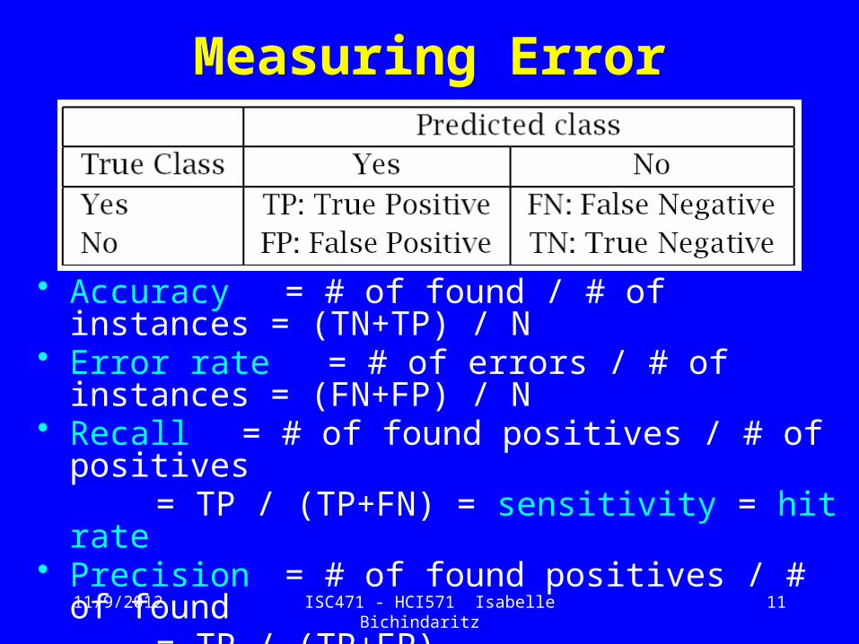
Measuring Error

• Accuracy = # of found / # of instances = (TN+TP) / N• Error rate = # of errors / # of instances = (FN+FP) / N• Recall = # of found positives / # of positives

= TP / (TP+FN) = sensitivity = hit rate• Precision = # of found positives / # of found

= TP / (TP+FP)• Specificity = TN / (TN+FP)• False alarm rate = FP / (FP+TN) = 1 - Specificity


12

ROC Curve

1/13/2010 TCSS888A Isabelle Bichindaritz 13

Approaches to Evaluating Classification

• Separate training (2/3) and testing (1/3) sets

• Use cross validation, e.g., 10-fold cross validation– Separate the data training (9/10) and testing (1/10)

– Repeat 10 times by rotating the (1/10) used for testing

– Average the results


14

• What is classification? What is prediction?

• Issues regarding classification and prediction



15

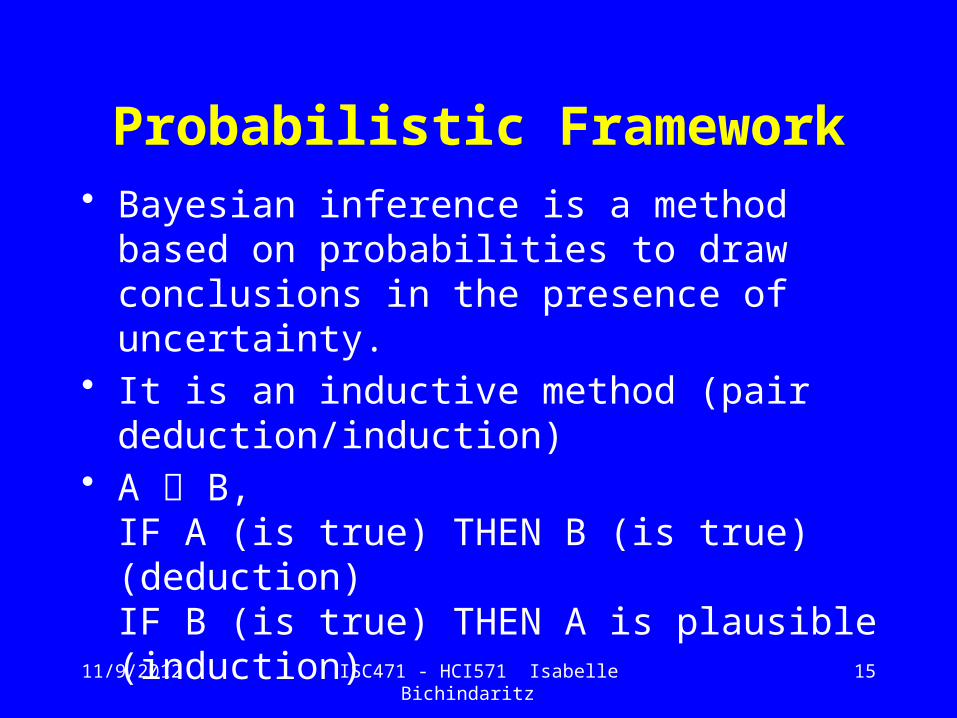
Probabilistic Framework• Bayesian inference is a method based on

probabilities to draw conclusions in the presence of uncertainty.

• It is an inductive method (pair deduction/induction)• A B,

IF A (is true) THEN B (is true) (deduction)IF B (is true) THEN A is plausible (induction)


16

Probabilistic Framework• Statistical framework

– State hypotheses and models (sets of hypotheses)

– Assign prior probabilities to the hypotheses

– Draw inferences using probability calculus: evaluate posterior probabilities (or degrees of belief) for the hypotheses given the data available, derive unique answers.


17

Probabilistic Framework

• Conditional probabilities (reads probability of X knowing Y):

• Events X and Y are said to be independent if:

)(

)()/(

YP

YXPYXP

)()/( XPYXP or)()()( YPXPYXP


18

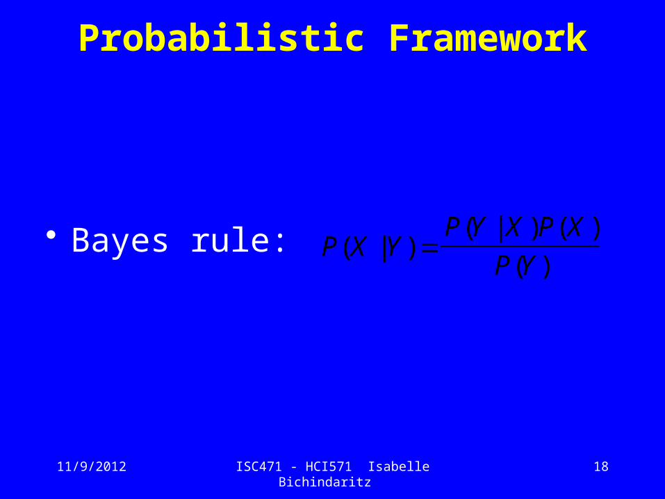
Probabilistic Framework

• Bayes rule:)(

)()|()|(

YP

XPXYPYXP


19

Bayesian Inference• Bayesian inference and induction consists in deriving a

model from a set of data– M is a model (hypotheses), D are the data– P(M|D) is the posterior - updated belief that M is correct– P(M) is our estimate that M is correct prior to any data– P(D|M) is the likelihood

– Logarithms are helpful to represent small numbers• Permits to combine prior knowledge with the

observed data.

)(

)()|()|(

DP

MPMDPDMP


20

Bayesian Inference• To be able to infer a model, we need to evaluate:

– The prior P(M)– The likelihood P(D/M)

• P(D) is calculated as the sum of all the numerators P(D/M)P(M) over all the hypotheses H, and thus we

do not need to calculate it:

M

MPMDP

MPMDPDMP

)()|(

)()|()|(


21

Bayesian Networks: Classification

diagnostic

P (C | x )

Bayes’ rule inverts the arc:

x

xx

pCPCp

CP|

|


22

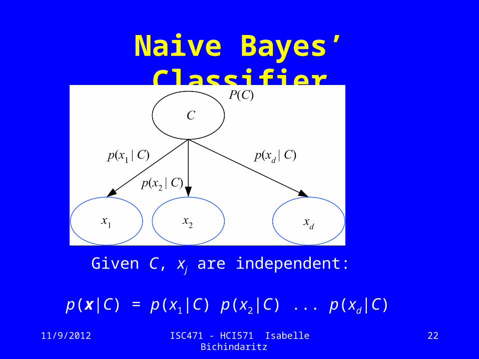
Naive Bayes’ Classifier

Given C, xj are independent:

p(x|C) = p(x1|C) p(x2|C) ... p(xd|C)


25

Bayesian classification• The classification problem may be formalized

using a-posteriori probabilities:• P(C|X) = prob. that the sample tuple

X=<x1,…,xk> is of class C.

• E.g. P(class=N | outlook=sunny,windy=true,…)

• Idea: assign to sample X the class label C such that P(C|X) is maximal


26

Estimating a-posteriori probabilities

• Bayes theorem:

P(C|X) = P(X|C)·P(C) / P(X)

• P(X) is constant for all classes

• P(C) = relative freq of class C samples

• C such that P(C|X) is maximum =

C such that P(X|C)·P(C) is maximum

• Problem: computing P(X|C) is unfeasible!


27

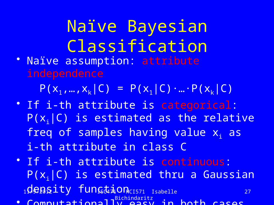
Naïve Bayesian Classification• Naïve assumption: attribute independence

P(x1,…,xk|C) = P(x1|C)·…·P(xk|C)

• If i-th attribute is categorical:P(xi|C) is estimated as the relative freq of samples having value xi as i-th attribute in class C

• If i-th attribute is continuous:P(xi|C) is estimated thru a Gaussian density function

• Computationally easy in both cases


28

Play-tennis example: estimating P(xi|C)

Outlook Temperature Humidity Windy Classsunny hot high false Nsunny hot high true Novercast hot high false Prain mild high false Prain cool normal false Prain cool normal true Novercast cool normal true Psunny mild high false Nsunny cool normal false Prain mild normal false Psunny mild normal true Povercast mild high true Povercast hot normal false Prain mild high true N

outlook

P(sunny|p) = 2/9 P(sunny|n) = 3/5

P(overcast|p) = 4/9 P(overcast|n) = 0

P(rain|p) = 3/9 P(rain|n) = 2/5

temperature

P(hot|p) = 2/9 P(hot|n) = 2/5

P(mild|p) = 4/9 P(mild|n) = 2/5

P(cool|p) = 3/9 P(cool|n) = 1/5

humidity

P(high|p) = 3/9 P(high|n) = 4/5

P(normal|p) = 6/9 P(normal|n) = 2/5

windy

P(true|p) = 3/9 P(true|n) = 3/5

P(false|p) = 6/9 P(false|n) = 2/5

P(p) = 9/14

P(n) = 5/14


29

Play-tennis example: classifying X

• An unseen sample X = <rain, hot, high, false>

• P(X|p)·P(p) = P(rain|p)·P(hot|p)·P(high|p)·P(false|p)·P(p) = 3/9·2/9·3/9·6/9·9/14 = 0.010582

• P(X|n)·P(n) = P(rain|n)·P(hot|n)·P(high|n)·P(false|n)·P(n) = 2/5·2/5·4/5·2/5·5/14 = 0.018286

• Sample X is classified in class n (don’t play)


30

The independence hypothesis…• … makes computation possible

• … yields optimal classifiers when satisfied

• … but is seldom satisfied in practice, as attributes

(variables) are often correlated.

• Attempts to overcome this limitation:– Bayesian networks, that combine Bayesian reasoning with

causal relationships between attributes

– Decision trees, that reason on one attribute at the time,

considering most important attributes first

11/9/2012ISC471 - HCI571 Isabelle Bichindaritz 1 Classification.

Documents

prediction classification

classification process

classification rules

training data observations

independent of training

set of measurements

training setthe model

observationsnew data