1.10 Normal Distribution

ROHINI COLLEGE OF ENGINEERING AND TECHNOLOGY

MA8451- PROBABILITY AND RANDOM PROCESSES

1.10 Normal Distribution

The Normal Probability Distribution is very common in the field of

statistics. Whenever you measure things like people's height, weight, salary,

opinions or votes, the graph of the results is very often a normal curve.

Properties of a Normal Distribution:

(i) The normal curve is symmetrical about the mean

(ii) The mean is at the middle and divides the area into halves.

(iii) The total area under the curve is equal to 1.

(iv) It is completely determined by its mean and standard deviation 𝜎 (or

variance 𝜎2).

Note:



In Normal distribution only two parameters are needed, namely 𝜇 and 𝜎2

Area under the Normal Curve using Integration:

The Probability of a continuous normal variable X found in a

particular interval [𝑎, 𝑏] is the area under the curve bounded by 𝑥 = 𝑎 and 𝑥 = 𝑏

is given by 𝑃(𝑎 < 𝑋 < 𝑏) = ∫ 𝑓(𝑋)𝑑𝑥𝑏

𝑎

and the area depends upon the values 𝜇 and 𝜎.

The standard Normal Distribution:

We standardize our normal curve, with a mean of zero and a standard

deviation of 1 unit.

If we have the standardized situation of 𝜇 = 0 and 𝜎 = 1 then we have

𝑓(𝑥) = 1

√2𝜋𝑒−𝑥2 2⁄



We can transform all the observations of any normal random variable X with mean

𝜇 and variance 𝜎 to a new set of observations of another normal random variable Z

with mean 0 and variance 1 using the following transformation:

𝑍 = 𝑋 − 𝜇

𝜎

The two graphs have different 𝜇 and 𝜎, but have the same area.

The new distribution of the normal random variable z with mean 0 and variance 1

(or standard deviation 1) is called a Standard normal distribution.

Formula for the Standardized normal Distribution

If we have mean 𝜇 and standard deviation 𝜎 , then

𝑍 = 𝑋 − 𝜇

𝜎

Find the moment generating function of Normal distribution

Sol: We first find the M.G.F of the standard normal distribution and hence find

mean and variance.

𝜙(𝑧) =1

√2𝜋𝑒

−𝑧2

2 ; −∞ < 𝑧 < ∞

where 𝑧 =𝑥−𝜇

𝜎

𝑀𝑧(𝑡) = 𝐸[𝑒𝑡𝑧]

= ∫−∞

∞ 𝑒𝑡𝑧𝜙(𝑧)𝑑𝑧



= ∫−∞

∞ 𝑒𝑡𝑧 1

√2𝜋𝑒

𝑧2

2 𝑑𝑧

=1

√2𝜋∫−∞

∞ 𝑒𝑡𝑧𝑒−

𝑧2

2 𝑑𝑧 =1

√2𝜋∫−∞

∞ 𝑒

(2𝑡𝑧−𝑧2

2)𝑑𝑧

=1

√2𝜋∫

−∞

∞ 𝑒

−(𝑧2−2𝑡𝑧

2)𝑑𝑧

=1

√2𝜋∫−∞

∞ 𝑒

−((𝑧−𝑡)2−𝑡2

2)𝑑𝑧 =

1

√2𝜋∫−∞

∞ 𝑒

−((𝑧−𝑡)2

2)+

𝑡2

2 𝑑𝑧

=1

√2𝜋∫−∞

∞ 𝑒

−((𝑧−𝑡)2

2)𝑒

𝑡2

2 𝑑𝑧

=𝑒

𝑡2

2

√2𝜋∫−∞

∞ 𝑒

−(𝑧−𝑡

√2)

2

𝑑𝑧 =𝑒

𝑡2

2

√2𝜋∫−∞

∞ 𝑒−𝑣2

√2𝑑𝑣

=𝑒

𝑡2

2

√𝜋∫

∞

−∞𝑒−𝑣2

𝑑𝑣 =𝑒

𝑡2

2

√𝜋√𝜋

𝑀𝑧(𝑡) = 𝑒𝑡2

2 … … … (1)

𝑀𝑋(𝑡) = 𝑀𝜇+𝜎𝑧(𝑡); ∑𝑧 =𝑋 − 𝜇

𝜎, 𝑋 = 𝜇 + 𝜎𝑧

= 𝑒𝜇𝑡𝑀𝑧(𝜎𝑡)

= 𝑒𝜇𝑡 ⋅ 𝑒𝜎2𝑡2

2 From (1)

= 𝑒𝜇𝑡+𝜎2𝑡2

2

To find mean and variance:

𝑀𝑋(𝑡) = 𝑒𝜇𝑡+𝜎2𝑡2

2



= 1 +𝜇𝑡+

𝜎2𝑡2

2

1!+

(𝜇𝑡+𝜎2𝑡2

2)

2

2!+ ⋯

= 1 +𝜇𝑡+

𝜎2𝑡2

2

1!+

(𝜇2𝑡2+𝜎4𝑡4

4+2𝜇𝑡

𝜎2𝑡2

2)

2!+ ⋯

Coefficient of 𝑡 = 𝜇 Coefficient of 𝑡2 =𝜎2

2+

𝜇2

2

𝐸(𝑋) = 1! × coefficient of 𝑡

= 𝜇

𝐸(𝑋2) = 2! × coefficient of 𝑡2

= 2 (𝜎2

2+

𝜇2

2) ⇒ 2 (

𝑒2+𝑢2

2)

= 𝜇2 + 𝜎2

variance = 𝐸(𝑋2) − [𝐸(𝑋)]2

= 𝜇2 + 𝜎2 − 𝜇2

= 𝜎2

Problems based on Normal distribution

1. X is normally distributed with mean 12 and SD is 4. Find the

probability that (i) 𝑿 ≥ 𝟐𝟎 (𝒊𝒊)𝑿 ≤ 𝟐𝟎 (𝒊𝒊𝒊)𝟎 ≤ 𝑿 ≤ 𝟏𝟐.

Solution:

Given X follows normally distribution with 𝝁 = 𝟏𝟐, 𝝈 = 𝟒

𝑃(𝑋 ≥ 20) = 𝑃 (𝑋−𝜇

𝜎≥

20−𝜇

𝜎) = 𝑃 (𝑍 ≥

20−12

4)



= 𝑃(𝑍 ≥ 2)

= 0.5 − 𝑃[0 < 𝑍 < 2]

= 0.5 − 0.4772 ( from the table)

𝑃(𝑋 ≥ 20) = 0.0228

(i) 𝑃(𝑋 ≤ 20) = 1 − 𝑃[ 𝑋 > 20] = 1 − 0.0228

𝑃(𝑋 ≤ 20) = 0.9772

(ii) 𝑃[0 ≤ 𝑋 ≤ 12] = 𝑃 (0−𝜇

𝜎≤

𝑋−𝜇

𝜎≥

12−𝜇

𝜎)

= 𝑃 (0 − 12

4≤ 𝑍 ≥

12 − 12

4)

= 𝑃(−3 ≤ 𝑍 ≤ 0)

= 𝑃(0 ≤ 𝑍 ≤ 3) (since the curve is symmetrical)

𝑃[0 ≤ 𝑋 ≤ 12] = 0.4987 (from the table)

2. In a normal distribution 31% of the items are under 45 and 8 % are

over 64. Find the mean and the standard deviation.

Solution:

Let the mean and standard deviation of the given normal distribution be 𝜇 and .

The area lying to the left of the ordinate at x = 45 is 0.31. The corresponding value

of z is negative.



The area lying to the right of the ordinates up to the mean is 0.5 – 0.31 = 0.19

The value of z corresponding to the area 0.19 is 0.5 nearly.

∴ 45−𝜇

𝜎= −0.5

(or) −0.5𝜎 + 𝜇 = 45 … … … … … … … … (1)

Area to the left of the ordinate at x = 64 is 0.5 – 0.08 = 0.42 and hence the value of

z corresponding to this area is 1.4 nearly.

∴ 64−𝜇

𝜎= 1.4

(or) 1.4𝜎 + 𝜇 = 64 … … … … … … … … . . (2)

Solving (1) and (2) we get

−0.5𝜎 + 𝜇 = 45

1.4𝜎 + 𝜇 = 64

(1) – (2) - 1.9𝜎 = - 19

⇒ 𝜎 = 10

Substituting 𝜎 = 10 in (1) we get

-0.5 (10) + 𝜇 = 45

-5 + 𝜇 = 45

⇒ 𝜇 = 50

3. The weekly wages of 1000 workmen are normally distributed around a

mean of Rs. 70 with a S.D of Rs. 5. Estimate the number of workers

whose weekly wages will be (i) between Rs.69 and Rs.72 (ii) less than

Rs.69 (iii) more than Rs.72



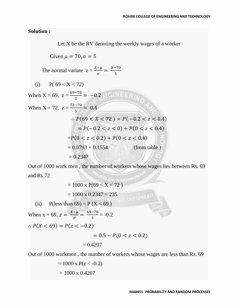
Solution :

Let X be the RV denoting the weekly wages of a worker

Given 𝜇 = 70, 𝜎 = 5

The normal variate z = 𝑋−𝜇

𝜎=

𝑋−70

5

(i) P( 69 < X < 72)

When X = 69, z = 69−70

5= −0.2

When X = 72, z = 72−70

5= 0.4

∴ 𝑃(69 < 𝑋 < 72 ) = 𝑃( −0.2 < 𝑧 < 0.4)

= 𝑃(−0.2 < 𝑧 < 0) + 𝑃(0 < 𝑧 < 0.4)

=𝑃(0 < 𝑧 < 0.2) + 𝑃(0 < 𝑧 < 0.4)

= 0.0793 + 0.1554 (from table )

= 0.2347

Out of 1000 work men , the number of workers whose wages lies between Rs. 69

and Rs.72

= 1000 x P(69 < X < 72 )

= 1000 x 0.2347 = 235

(ii) P(less than 69) = P (X < 69 )

When x = 69, 𝑧 = 𝑋−𝜇

𝜎=

69−70

5 = -0.2

∴ 𝑃(𝑋 < 69) = 𝑃(𝑧 < −0.2)

= 0.5 − 𝑃(0 < 𝑧 < 0.2)

= 0.4207

Out of 1000 workmen , the number of workers whose wages are less than Rs. 69

= 1000 x P(z < -0.2)

= 1000 x 0.4207



= 420.7

(iii) P( more than Rs. 72 ) = P(X > 72)

When x = 72, 𝑧 = 𝑋−𝜇

𝜎=

72−70

5 = -0.2

∴ 𝑃(𝑋 < 69) = 𝑃(𝑧 < −0.2)

= 0.5 − 𝑃(0 < 𝑧 < 0.2)

= 0.4207

Out of 1000 workmen , the number of workers whose wages are less than Rs. 69

= 1000 x P(z < -0.2)

= 1000 x 0.4207

= 420.7



1.10 Normal Distribution

Documents