11 PISA 2015 TECHNICAL REPORT © OECD 2017 203 Sampling outcomes Population coverage............................................................................................... 204 School and student response rates ........................................................................ 205 Teacher response rates ........................................................................................... 214 Design effects and effective sample sizes ............................................................. 215 Variability of the design effect ............................................................................... 217 The statistical data for Israel are supplied by and under the responsibility of the relevant Israeli authorities. The use of such data by the OECD is without prejudice to the status of the Golan Heights, East Jerusalem and Israeli settlements in the West Bank under the terms of international law.

Welcome message from author
This document is posted to help you gain knowledge. Please leave a comment to let me know what you think about it! Share it to your friends and learn new things together.
Transcript
11
PISA 2015 TECHNICAL REPORT © OECD 2017 203
Sampling outcomes
Population coverage ............................................................................................... 204
School and student response rates ........................................................................ 205
Teacher response rates ........................................................................................... 214
Design effects and effective sample sizes ............................................................. 215
Variability of the design effect ............................................................................... 217
The statistical data for Israel are supplied by and under the responsibility of the relevant Israeli authorities. The use of such data by the OECD is without prejudice to the status of the Golan Heights, East Jerusalem and Israeli settlements in the West Bank under the terms of international law.
11SAMPLING OUTCOMES
204 © OECD 2017 PISA 2015 TECHNICAL REPORT
This chapter reports on PISA sampling outcomes. Details of the sample design are provided in Chapter 4.
POPULATION COVERAGETables 11.1 and 11.2 (by adjudicated regions) show the quality indicators for population coverage and the information used to develop them. The following notes explain the meaning of each coverage index and how the data in each column of the table were used.
Coverage indices 1, 2 and 3 are intended to measure PISA population coverage. Coverage indices 4 and 5 are intended to be diagnostic in cases where indices 1, 2 or 3 have unexpected values. Many references are made in this chapter to the various sampling tasks on which National Project Managers (NPMs) documented statistics and other information needed in undertaking the sampling of schools and students. Note that although no comparison is made between the total population of 15-year-olds and the enrolled population of 15-year-old students, generally the enrolled population was expected to be less than or equal to the total population. Occasionally this was not the case due to differing data sources for these two values.
Coverage index 1: Coverage of the national population, calculated by P/(P + E) × (ST7b_3/ST7b_1):
• Coverage index 1 shows the extent to which the weighted participants covered the final target population after all school exclusions. The following bullet points give details of its computation.
• In the preceding expression P/(P + E) broadly represents the coverage proportion due to within-school exclusion, and (ST7b_3/ST7b_1) the coverage proportion due to school-level exclusion.
• The national population value, defined by sampling task 7b response box [1] and denoted here as ST7b_1 (and in Table 11.1 as the target population) is the population that includes all enrolled 15-year-old students in grades 7 and above in each participating country (with the possibility of small levels of exclusions), based on national statistics. However, the final national population value reflected for each country’s school sampling frame might have had some school-level exclusions. The value that represents the population of enrolled 15-year-old students minus those in excluded schools is represented initially by response box [3] on sampling task 7b. It is denoted here as ST7b_3. As in PISA 2012, the procedure for PISA 2015 was that small schools having only one or two PISA-eligible students could not be excluded from the school frame but could be excluded in the field if the school still had only one or two PISA-eligible students at the time of data collection. Therefore, what is noted in coverage index 1 as ST7b_3 (and in Table 11.1 as target minus school-level exclusions) was a number after accounting for all school-level exclusions, which means a number that omits schools excluded from the sampling frame in addition to those schools excluded in the field. Thus, the term (ST7b_3/ST7b_1) provides the proportion of the national population covered in each country based on national statistics.
• The value (P + E) provides the weighted estimate from the student sample of all PISA-eligible 15-year-olds in each participating country, where P is the weighted estimate of PISA-eligible non-excluded 15-year-old students and E is the weighted estimate of PISA-eligible 15-year-old students that were excluded within schools. Therefore, the term P/(P + E) provides an estimate, based on the student sample, of the proportion of the PISA-eligible 15-year-old population represented by the non-excluded PISA-eligible 15-year-old students.
• The result of multiplying these two proportions together P/(P + E) and (ST7b_3/ST7b_1) indicates the overall proportion of the national population covered by the non-excluded portion of the student sample.
Coverage index 2: Coverage of the national enrolled population, calculated by P/(P + E) × (ST7b_3/ST7a_2.1):
• Coverage index 2 shows the extent to which the weighted participants covered the target population of all enrolled students in grades 7 and above.
• The national enrolled population (NEP), defined by sampling task 7a response box [2.1] and denoted here as ST7a_2.1 (and as enrolled 15-year-old students in Table 11.1), is the population that includes all enrolled 15-year-old students in grades 7 and above in each participating country, based on national statistics. The final national population, denoted here as ST7b_3 as described above for coverage index 1, reflects the 15-year-old population after school-level and other small exclusions. This value represents the population of enrolled 15-year-old students less those in excluded schools.
• The value (P + E) provides the weighted estimate from the student sample of all eligible 15-year-olds in each country, where P is the weighted estimate of PISA-eligible non-excluded 15-year-old students and E is the weighted estimate of PISA-eligible 15-year-old students that were excluded within schools. Therefore, the term P/(P + E) provides an

11SAMPLING OUTCOMES
PISA 2015 TECHNICAL REPORT © OECD 2017 205
estimate based on the student sample of the proportion of the PISA-eligible 15-year-old population that is represented by the non-excluded PISA-eligible 15-year-old students.
• Multiplying these two proportions together (P/(P + E) and (ST7b_3/ST7a_2.1)) gives the overall proportion of the NEP that was covered by the non-excluded portion of the student sample.
Coverage index 1 and coverage index 2 will differ when countries have excluded geographical areas or language groups apart from other school-level exclusions. In these cases coverage index 2 will be less than coverage index 1.
Coverage index 3: Coverage of the national 15-year-old population, calculated by P/ST7a_1:
• The national population of 15-year-olds, defined by sampling task 7a response box [1] and denoted here as ST7a_1 (and called all 15-year-olds in Table 11.1), is the entire population of 15-year-olds in each country (enrolled and not enrolled), based on national statistics. The value P is the weighted estimate of PISA-eligible non-excluded 15-year-old students from the student sample. Thus (P/ST7a_1) indicates the proportion of the national population of 15-year-olds covered by the non-excluded portion of the student sample. It therefore also reflects the proportion of 15-year-olds excluded or not at school.
Coverage index 4: Coverage of the estimated school population, calculated by (P + E)/S:
• The value (P + E) provides the weighted estimate from the student sample of all PISA-eligible 15-year-old students in each country, where P is the weighted estimate of PISA-eligible non-excluded 15-year-old students and E is the weighted estimate of PISA-eligible 15-year-old students who were excluded within schools.
• The value S is an estimate of the 15-year-old school population in each participating country (called estimate of enrolled students from frame in Table 11.1). This is based on the actual or (more often) approximate number of 15-year-old students enrolled in each school in the sample, prior to contacting the school to conduct the assessment. The S value is calculated as the sum over all sampled schools of the product of each school’s sampling weight and its number of 15-year-old students (ENR) as recorded on the school sampling frame.
• Thus, (P + E)/S is the proportion of the estimated school 15-year-old population that is represented by the weighted estimate from the student sample of all PISA-eligible 15-year-old students. It is influenced by the accuracy of the school sample frame, fluctuations in the target population size and the accuracy of the within-school sampling process. Its purpose is to check whether the student sampling has been carried out correctly, and to assess whether the value of S is a reliable measure of the number of enrolled 15-year-olds. This is important for interpreting coverage index 5.
Coverage index 5: Coverage of the school sampling frame population, calculated by S/ST7b_3:
• The value (S/ST7b_3) is the ratio of the enrolled 15-year-old population, as estimated from data on the school sampling frame, to the size of the enrolled student population, as reported on sampling task 7b and adjusted by removing any additional excluded schools in the field. In some cases, this provided a check as to whether the data on the sampling frame gave a reliable estimate of the number of 15-year-old students in each school. In other cases, however, it was evident that ST7b_3 had been derived using data from the sampling frame by the NPM, so that this ratio may have been close to 1.0 even if enrolment data on the school sampling frame were poor. Under such circumstances, coverage index 4 would differ noticeably from 1.0, and the figure for ST7b_3 would also be inaccurate.
SCHOOL AND STUDENT RESPONSE RATESTables 11.3 to 11.8 present school and student-level response rates at the national and regional levels.
• Tables 11.3 and 11.4 (by adjudicated regions) indicate the rates calculated by using only original schools and no replacement schools.
• Tables 11.5 and 11.6 (by adjudicated regions) indicate the improved response rates when first and second replacement schools were accounted for in the rates.
• Tables 11.7 and 11.8 (by adjudicated regions) indicate the student response rates among the full set of participating schools.

11SAMPLING OUTCOMES
206 © OECD 2017 PISA 2015 TECHNICAL REPORT
Table 11.1[Part 1/2]PISA target populations and samples
All 15-year-
olds
Enrolled 15-year-
oldsTarget
populationSchool-level exclusions
Target minus school level exclusions
School level exclusion rate (%)
Estimation of enrolled
students from frame
Number of participating
students
Weighted number of
participating students
Number of excluded students
OEC
D Australia 282 888 282 547 282 547 6 940 275 607 2.46 276 072 14 530 256 329 681Austria 88 013 82 683 82 683 790 81 893 0.96 81 730 7 007 73 379 84Belgium 123 630 121 954 121 694 1 597 120 097 1.31 118 915 9 651 114 902 39Canada 396 966 381 660 376 994 1 590 375 404 0.42 381 133 20 058 331 546 1 830Chile 255 440 245 947 245 852 2 641 243 211 1.07 232 756 7 053 203 782 37Czech Republic 90 391 90 076 90 076 1 814 88 262 2.01 87 999 6 894 84 519 25Denmark 68 174 67 466 67 466 605 66 861 0.90 63 897 7 161 60 655 514Estonia 11 676 11 491 11 491 416 11 075 3.62 11 154 5 587 10 834 116Finland 58 526 58 955 58 955 472 58 483 0.80 58 782 5 882 56 934 124France 807 867 778 679 778 679 28 742 749 937 3.69 749 284 6 108 734 944 35Germany 774 149 774 149 774 149 11 150 762 999 1.44 794 206 6 522 743 969 54Greece 105 530 105 253 105 253 953 104 300 0.91 103 031 5 532 96 157 58Hungary 94 515 90 065 90 065 1 945 88 120 2.16 89 808 5 658 84 644 55Iceland 4 250 4 195 4 195 17 4 178 0.41 4 163 3 374 3 966 131Ireland 61 234 59 811 59 811 72 59 739 0.12 61 461 5 741 59 082 197Israel 124 852 118 997 118 997 2 310 116 687 1.94 115 717 6 598 117 031 115Italy 616 761 567 268 567 268 11 190 556 078 1.97 516 113 11 583 495 093 246Japan 1 201 615 1 175 907 1 175 907 27 323 1 148 584 2.32 1 151 305 6 647 1 138 349 2Korea 620 687 619 950 619 950 3 555 616 395 0.57 615 107 5 581 569 106 20Latvia 17 255 16 955 16 955 677 16 278 3.99 16 334 4 869 15 320 70Luxembourg 6 327 6 053 6 053 162 5 891 2.68 5 891 5 299 5 540 331Mexico 2 257 399 1 401 247 1 401 247 5 905 1 395 342 0.42 1 373 919 7 568 1 392 995 30Netherlands 201 670 200 976 200 976 6 866 194 110 3.42 191 966 5 385 191 817 14New Zealand 60 162 57 448 57 448 681 56 767 1.19 56 875 4 520 54 274 333Norway 63 642 63 491 63 491 854 62 637 1.35 61 809 5 456 58 083 345Poland 380 366 361 600 361 600 6 122 355 478 1.69 355 158 4 478 345 709 34Portugal 110 939 101 107 101 107 424 100 683 0.42 102 193 7 325 97 214 105Slovak Republic 55 674 55 203 55 203 1 376 53 827 2.49 54 499 6 350 49 654 114Slovenia 18 078 17 689 17 689 290 17 399 1.64 17 286 6 406 16 773 114Spain 440 084 414 276 414 276 2 175 412 101 0.53 409 246 6 736 399 935 200Sweden 97 749 97 210 97 210 1 214 95 996 1.25 94 097 5 458 91 491 275Switzerland 85 495 83 655 83 655 2 320 81 335 2.77 81 026 5 860 82 223 107Turkey 1 324 089 1 100 074 1 100 074 5 746 1 094 328 0.52 1 091 317 5 895 925 366 31United Kingdom 747 593 746 328 746 328 23 412 722 916 3.14 707 415 14 157 627 703 870United States 4 220 325 3 992 053 3 992 053 12 001 3 980 052 0.30 3 902 089 5 712 3 524 497 193
Part
ners Albania 48 610 45 163 45 163 10 45 153 0.02 43 919 5 215 40 896 0
Algeria 389 315 354 936 354 936 354 936 0.00 355 216 5 519 306 647 0Argentina 718 635 578 308 578 308 2 617 575 691 0.45 572 941 6 349 394 917 21Brazil 3 803 681 2 853 388 2 853 388 64 392 2 788 996 2.26 2 692 686 23 141 2 425 961 119B-S-J-G (China)* 2 084 958 1 507 518 1 507 518 58 639 1 448 879 3.89 1 437 201 9 841 1 331 794 33Bulgaria 66 601 59 397 59 397 1 124 58 273 1.89 56 483 5 928 53 685 49Colombia 760 919 674 079 674 079 37 674 042 0.01 673 817 11 795 567 848 9Costa Rica 81 773 66 524 66 524 66 524 0.00 67 073 6 866 51 897 13Croatia 45 031 35 920 35 920 805 35 115 2.24 34 652 5 809 40 899 86Cyprus1 9 255 9 255 9 253 109 9 144 1.18 9 126 5 571 8 785 228Dominican Republic 193 153 139 555 139 555 2 382 137 173 1.71 138 187 4 740 132 300 4FYROM 16 719 16 717 16 717 259 16 458 1.55 16 472 5 324 15 847 8Georgia 48 695 43 197 43 197 1 675 41 522 3.88 41 595 5 316 38 334 35Hong Kong (China) 65 100 61 630 61 630 708 60 922 1.15 60 716 5 359 57 662 36Indonesia 4 534 216 3 182 816 3 182 816 4 046 3 178 770 0.13 3 176 076 6 513 3 092 773 0Jordan 126 399 121 729 121 729 71 121 658 0.06 119 024 7 267 108 669 70Kazakhastan 211 407 209 555 209 555 7 475 202 080 3.57 202 701 7 841 192 909 0Kosovo 31 546 28 229 28 229 1 156 27 073 4.10 26 924 4 826 22 333 50Lebanon 64 044 62 281 62 281 1 300 60 981 2.09 60 882 4 546 42 331 0Lithuania 33 163 32 097 32 097 573 31 524 1.79 31 588 6 525 29 915 227Macao (China) 5 100 4 417 4 417 3 4 414 0.07 4 414 4 476 4 507 0Malaysia 540 000 448 838 448 838 2 418 446 420 0.54 446 237 8 861 412 524 41Malta 4 397 4 406 4 406 63 4 343 1.43 4 343 3 634 4 296 41Moldova 31 576 30 601 30 601 182 30 419 0.59 30 145 5 325 29 341 21Montenegro 7 524 7 506 7 506 40 7 466 0.53 7 312 5 665 6 777 300Peru 580 371 478 229 478 229 6 355 471 874 1.33 470 651 6 971 431 738 13Qatar 13 871 13 850 13 850 380 13 470 2.74 13 470 12 083 12 951 193Romania 176 334 176 334 176 334 1 823 174 511 1.03 172 652 4 876 164 216 3Russian Federation 1 176 473 1 172 943 1 172 943 24 217 1 148 726 2.06 1 189 441 6 036 1 120 932 13Singapore 48 218 47 050 47 050 445 46 605 0.95 46 620 6 115 46 224 25Chinese Taipei 295 056 287 783 287 783 1 179 286 604 0.41 286 778 7 708 251 424 22Thailand 895 513 756 917 756 917 9 646 747 271 1.27 751 010 8 249 634 795 22Trinidad and Tobago 17 371 17 371 17 371 17 371 0.00 17 371 4 692 13 197 0Tunisia 122 186 122 186 122 186 679 121 507 0.56 122 767 5 375 113 599 3United Arab Emirates 51 687 51 518 51 499 994 50 505 1.93 50 060 14 167 46 950 63Uruguay 53 533 43 865 43 865 4 43 861 0.01 43 737 6 062 38 287 6Viet Nam 1 803 552 1 032 599 1 032 599 6 557 1 026 042 0.63 996 757 5 826 874 859 0
* B-S-J-G (China) refers to the four PISA-participating China provinces: Beijing, Shanghai, Jiangsu and Guangdong. 1. Note by Turkey: The information in this document with reference to ”Cyprus” relates to the southern part of the Island. There is no single authority representing both Turkish and Greek Cypriot people on the Island. Turkey recognises the Turkish Republic of Northern Cyprus (TRNC). Until a lasting and equitable solution is found within the context of the United Nations, Turkey shall preserve its position concerning the “Cyprus issue”.Note by all the European Union Member States of the OECD and the European Union: The Republic of Cyprus is recognised by all members of the United Nations with the exception of Turkey. The information in this document relates to the area under the effective control of the Government of the Republic of Cyprus.

11SAMPLING OUTCOMES
PISA 2015 TECHNICAL REPORT © OECD 2017 207
Table 11.1[Part 2/2]PISA target populations and samples
Weighted number of excluded students
Number of ineligible students
Weighted number of ineligible students
Within-school
exclusion rate (%)
Overall exclusion rate (%)
Percentage of ineligible /
withdrawnCoverage Index 1
Coverage Index 2
Coverage Index 3
Coverage Index 4
Coverage Index 5
OEC
D Australia 7 736 904 8 203 2.93 5.31 3.11 0.95 0.95 0.91 0.96 1.00Austria 866 669 3 431 1.17 2.11 4.62 0.98 0.98 0.83 0.91 1.00Belgium 410 147 1 576 0.36 1.66 1.37 0.98 0.98 0.93 0.97 0.99Canada 25 340 864 9 513 7.10 7.49 2.67 0.93 0.91 0.84 0.94 1.02Chile 1 393 114 3 782 0.68 1.75 1.84 0.98 0.98 0.80 0.88 0.96Czech Republic 368 82 825 0.43 2.44 0.97 0.98 0.98 0.94 0.96 1.00Denmark 2 644 48 289 4.18 5.04 0.46 0.95 0.95 0.89 0.99 0.96Estonia 218 34 61 1.97 5.52 0.55 0.94 0.94 0.93 0.99 1.01Finland 1 157 13 124 1.99 2.78 0.21 0.97 0.97 0.97 0.99 1.01France 3 620 157 16 455 0.49 4.16 2.23 0.96 0.96 0.91 0.99 1.00Germany 5 342 110 11 334 0.71 2.14 1.51 0.98 0.98 0.96 0.94 1.04Greece 965 87 1 616 0.99 1.89 1.66 0.98 0.98 0.91 0.94 0.99Hungary 1 009 48 769 1.18 3.31 0.90 0.97 0.97 0.90 0.95 1.02Iceland 132 179 181 3.23 3.62 4.40 0.96 0.96 0.93 0.98 1.00Ireland 1 825 117 1 033 3.00 3.11 1.70 0.97 0.97 0.96 0.99 1.03Israel 1 803 78 1 323 1.52 3.43 1.11 0.97 0.97 0.94 1.03 0.99Italy 9 395 305 11 766 1.86 3.80 2.33 0.96 0.96 0.80 0.98 0.93Japan 318 12 1 868 0.03 2.35 0.16 0.98 0.98 0.95 0.99 1.00Korea 1 806 65 6 268 0.32 0.89 1.10 0.99 0.99 0.92 0.93 1.00Latvia 174 153 430 1.12 5.07 2.77 0.95 0.95 0.89 0.95 1.00Luxembourg 331 24 24 5.64 8.16 0.41 0.92 0.92 0.88 1.00 1.00Mexico 6 810 505 84 669 0.49 0.91 6.05 0.99 0.99 0.62 1.02 0.98Netherlands 502 20 592 0.26 3.67 0.31 0.96 0.96 0.95 1.00 0.99New Zealand 3 112 114 1 102 5.42 6.54 1.92 0.93 0.93 0.90 1.01 1.00Norway 3 366 43 445 5.48 6.75 0.72 0.93 0.93 0.91 0.99 0.99Poland 2 418 22 1 505 0.69 2.38 0.43 0.98 0.98 0.91 0.98 1.00Portugal 860 239 2 699 0.88 1.29 2.75 0.99 0.99 0.88 0.96 1.01Slovak Republic 912 130 999 1.80 4.25 1.98 0.96 0.96 0.89 0.93 1.01Slovenia 247 75 144 1.45 3.07 0.84 0.97 0.97 0.93 0.98 0.99Spain 10 893 45 2 366 2.65 3.16 0.58 0.97 0.97 0.91 1.00 0.99Sweden 4 324 46 715 4.51 5.71 0.75 0.94 0.94 0.94 1.02 0.98Switzerland 1 357 146 1 659 1.62 4.35 1.99 0.96 0.96 0.96 1.03 1.00Turkey 5 359 533 73 779 0.58 1.10 7.93 0.99 0.99 0.70 0.85 1.00United Kingdom 34 747 297 8 914 5.25 8.22 1.35 0.92 0.92 0.84 0.94 0.98United States 109 580 330 191 378 3.02 3.31 5.27 0.97 0.97 0.84 0.93 0.98
Part
ners Albania 0 0 0 0.00 0.02 0.00 1.00 1.00 0.84 0.93 0.97
Algeria 0 0 0 0.00 0.00 0.00 1.00 1.00 0.79 0.86 1.00Argentina 1 367 204 11 847 0.34 0.80 2.99 0.99 0.99 0.55 0.69 1.00Brazil 13 543 1 582 143 969 0.56 2.80 5.90 0.97 0.97 0.64 0.91 0.97B-S-J-G (China) 3 609 552 94 478 0.27 4.15 7.07 0.96 0.96 0.64 0.93 0.99Bulgaria 433 74 681 0.80 2.68 1.26 0.97 0.97 0.81 0.96 0.97Colombia 507 621 30 813 0.09 0.09 5.42 1.00 1.00 0.75 0.84 1.00Costa Rica 98 400 3 154 0.19 0.19 6.07 1.00 1.00 0.63 0.78 1.01Croatia 589 73 456 1.42 3.63 1.10 0.96 0.96 0.91 1.20 0.99Cyprus1 292 89 114 3.22 4.36 1.25 0.96 0.96 0.95 0.99 1.00Dominican Republic 106 102 2 500 0.08 1.79 1.89 0.98 0.98 0.68 0.96 1.01FYROM 19 162 451 0.12 1.67 2.84 0.98 0.98 0.95 0.96 1.00Georgia 230 72 515 0.60 4.45 1.34 0.96 0.96 0.79 0.93 1.00Hong Kong (China) 374 10 102 0.65 1.79 0.18 0.98 0.98 0.89 0.96 1.00Indonesia 0 261 124 725 0.00 0.13 4.03 1.00 1.00 0.68 0.97 1.00Jordan 1 006 448 6 256 0.92 0.97 5.70 0.99 0.99 0.86 0.92 0.98Kazakhastan 0 0 0 0.00 3.57 0.00 0.96 0.96 0.91 0.95 1.00Kosovo 174 215 1 010 0.77 4.84 4.49 0.95 0.95 0.71 0.84 0.99Lebanon 0 0 0 0.00 2.09 0.00 0.98 0.98 0.66 0.70 1.00Lithuania 1 050 68 282 3.39 5.12 0.91 0.95 0.95 0.90 0.98 1.00Macao (China) 0 28 28 0.00 0.07 0.62 1.00 1.00 0.88 1.02 1.00Malaysia 2 344 232 13 167 0.56 1.10 3.17 0.99 0.99 0.76 0.93 1.00Malta 41 9 9 0.95 2.36 0.21 0.98 0.98 0.98 1.00 1.00Moldova 118 34 194 0.40 0.99 0.66 0.99 0.99 0.93 0.98 0.99Montenegro 332 72 78 4.66 5.17 1.10 0.95 0.95 0.90 0.97 0.98Peru 745 329 20 685 0.17 1.50 4.78 0.99 0.99 0.74 0.92 1.00Qatar 193 389 392 1.47 4.17 2.99 0.96 0.96 0.93 0.98 1.00Romania 120 117 3 991 0.07 1.11 2.43 0.99 0.99 0.93 0.95 0.99Russian Federation 2 469 32 5 732 0.22 2.28 0.51 0.98 0.98 0.95 0.94 1.04Singapore 179 51 303 0.39 1.33 0.65 0.99 0.99 0.96 1.00 1.00Chinese Taipei 647 80 2 420 0.26 0.67 0.96 0.99 0.99 0.85 0.88 1.00Thailand 2 107 424 36 993 0.33 1.60 5.81 0.98 0.98 0.71 0.85 1.01Trinidad and Tobago 0 206 421 0.00 0.00 3.19 1.00 1.00 0.76 0.76 1.00Tunisia 61 144 2 592 0.05 0.61 2.28 0.99 0.99 0.93 0.93 1.01United Arab Emirates 152 170 714 0.32 2.25 1.52 0.98 0.98 0.91 0.94 0.99Uruguay 32 522 2 900 0.08 0.09 7.57 1.00 1.00 0.72 0.88 1.00Viet Nam 0 144 24 954 0.00 0.63 2.85 0.99 0.99 0.49 0.88 0.97
1. Note by Turkey: The information in this document with reference to ”Cyprus” relates to the southern part of the Island. There is no single authority representing both Turkish and Greek Cypriot people on the Island. Turkey recognises the Turkish Republic of Northern Cyprus (TRNC). Until a lasting and equitable solution is found within the context of the United Nations, Turkey shall preserve its position concerning the “Cyprus issue”.Note by all the European Union Member States of the OECD and the European Union: The Republic of Cyprus is recognised by all members of the United Nations with the exception of Turkey. The information in this document relates to the area under the effective control of the Government of the Republic of Cyprus.

11SAMPLING OUTCOMES
208 © OECD 2017 PISA 2015 TECHNICAL REPORT
Table 11.2[Part 1/2]PISA target populations and samples, by adjudicated regions
All 15-year-
olds
Enrolled 15-year-
oldsTarget
populationSchool-level exclusions
Target minus school level exclusions
School level
exclusion rate (%)
Estimation of enrolled
students from frame
Number of participating
students
Weighted number of
participating students
Number of excluded students
OEC
D Belgium (Flemish community) 70 451 68 173 68 173 997 67 176 1.46 65 298 5 675 62 986 16Spain (Andalusia) 88 493 82 495 82 495 251 82 244 0.30 82 193 1 813 81 642 44Spain (Aragon) 11 737 11 192 11 192 48 11 144 0.43 11 126 1 798 10 758 38Spain (Asturias) 7 391 7 186 7 186 27 7 159 0.38 7 066 1 790 6 895 24Spain (Balearic Islands) 10 629 9 623 9 623 60 9 563 0.63 9 502 1 797 9 208 38Spain (Basque Country) 18 455 18 117 18 117 60 18 057 0.33 18 113 3 612 17 424 64Spain (Canary Islands) 21 848 20 192 20 192 70 20 122 0.35 20 229 1 842 19 447 40Spain (Cantabria) 4 821 4 775 4 775 19 4 756 0.40 4 780 1 924 4 576 17Spain (Castile and Leon) 20 057 19 690 19 690 84 19 606 0.43 19 602 1 858 18 004 98Spain (CastileLaMancha) 21 165 19 646 19 646 115 19 531 0.59 19 543 1 889 19 247 35Spain (Catalonia) 70 633 68 278 68 278 612 67 666 0.90 67 606 1 769 63 112 92Spain (Extremadura) 10 955 10 745 10 745 64 10 681 0.60 10 592 1 809 10 054 40Spain (Galicia) 20 949 19 616 19 616 69 19 547 0.35 19 617 1 865 19 063 45Spain (La Rioja) 2 934 2 853 2 853 33 2 820 1.16 2 822 1 461 2 758 5Spain (Madrid) 58 569 53 865 53 865 383 53 482 0.71 53 137 1 808 53 240 21Spain (Murcia) 15 690 14 044 14 044 62 13 982 0.44 14 015 1 796 13 555 60Spain (Navarra) 6 192 5 856 5 856 27 5 829 0.46 5 793 1 874 5 496 53Spain (Valencia) 47 367 44 072 44 072 198 43 874 0.45 43 204 1 625 38 900 144United Kingdom (Scotland) 56 171 56 344 56 344 897 55 447 1.59 55 282 3 111 50 190 207United States (Massachusetts (public)) 80 631 82 745 71 900 18 71 882 0.03 69 899 1 652 60 918 81United States (North Carolina (public)) 130 833 116 807 110 215 416 109 799 0.38 110 786 1 887 104 161 89United States (Puerto Rico)1 50 321 44 613 44 613 760 43 853 1.70 39 453 1 398 30 261 24
Part
ners Argentina (CABA) 30 974 35 767 35 767 12 35 755 0.03 35 576 1 657 32 180 6
United Arab Emirates (Abu Dhabi) 19 702 19 629 19 611 204 19 407 1.04 19 402 3 610 18 335 8
United Arab Emirates (Dubai) 14 662 14 643 14 642 579 14 063 3.95 14 057 6 287 12 906 51
1. Puerto Rico is an unincorporated territory of the United States. As such, PISA results for the United States do not include Puerto Rico.
Table 11.2[Part 2/2]PISA target populations and samples, by adjudicated regions
Weighted number of excluded students
Number of ineligible students
Weighted number of ineligible students
Within-school
exclusion rate (%)
Overall exclusion rate (%)
Percentage of ineligible /
withdrawnCoverage Index 1
Coverage Index 2
Coverage Index 3
Coverage Index 4
Coverage Index 5
OEC
D Belgium (Flemish community) 159 79 780 0.25 1.71 1.24 0.98 0.98 0.89 0.97 0.97Spain (Andalusia) 1 718 21 817 2.06 2.36 0.98 0.98 0.98 0.92 1.01 1.00Spain (Aragon) 204 20 112 1.86 2.28 1.02 0.98 0.98 0.92 0.99 1.00Spain (Asturias) 84 8 27 1.21 1.58 0.39 0.98 0.98 0.93 0.99 0.99Spain (Balearic Islands) 177 9 40 1.89 2.50 0.43 0.98 0.98 0.87 0.99 0.99Spain (Basque Country) 254 20 67 1.44 1.76 0.38 0.98 0.98 0.94 0.98 1.00Spain (Canary Islands) 374 29 285 1.89 2.23 1.44 0.98 0.98 0.89 0.98 1.01Spain (Cantabria) 35 8 19 0.76 1.15 0.41 0.99 0.99 0.95 0.96 1.01Spain (Castile and Leon) 883 14 123 4.67 5.08 0.65 0.95 0.95 0.90 0.96 1.00Spain (CastileLaMancha) 333 22 213 1.70 2.28 1.09 0.98 0.98 0.91 1.00 1.00Spain (Catalonia) 3 011 18 578 4.55 5.41 0.87 0.95 0.95 0.89 0.98 1.00Spain (Extremadura) 201 18 92 1.96 2.54 0.89 0.97 0.97 0.92 0.97 0.99Spain (Galicia) 417 3 28 2.14 2.48 0.14 0.98 0.98 0.91 0.99 1.00Spain (La Rioja) 7 27 48 0.26 1.41 1.73 0.99 0.99 0.94 0.98 1.00Spain (Madrid) 529 11 270 0.98 1.69 0.50 0.98 0.98 0.91 1.01 0.99Spain (Murcia) 391 4 27 2.80 3.23 0.20 0.97 0.97 0.86 1.00 1.00Spain (Navarra) 138 18 48 2.45 2.90 0.86 0.97 0.97 0.89 0.97 0.99Spain (Valencia) 3 014 12 247 7.19 7.61 0.59 0.92 0.92 0.82 0.97 0.98United Kingdom (Scotland) 2 645 172 2 166 5.01 6.52 4.10 0.93 0.93 0.89 0.96 1.00United States (Massachusetts (public)) 2 785 106 3 514 4.37 4.40 5.52 0.96 0.83 0.76 0.91 0.97United States (North Carolina (public)) 4 636 107 5 517 4.26 4.62 5.07 0.95 0.90 0.80 0.98 1.01United States (Puerto Rico)1 440 235 8 761 1.43 3.11 28.54 0.97 0.97 0.60 0.78 0.90
Part
ners Argentina (CABA) 85 48 714 0.26 0.30 2.21 1.00 1.00 1.04 0.91 0.99
United Arab Emirates (Abu Dhabi) 36 53 265 0.19 1.23 1.44 0.99 0.99 0.93 0.95 1.00
United Arab Emirates (Dubai) 104 69 215 0.80 4.72 1.65 0.95 0.95 0.88 0.93 1.00
1. Puerto Rico is an unincorporated territory of the United States. As such, PISA results for the United States do not include Puerto Rico.
For calculating school response rates before replacement, the numerator consisted of all original sample schools with enrolled age-eligible students who participated (i.e., assessed a sample of PISA-eligible students, and obtained a student response rate of at least 50%). The denominator consisted of all the schools in the numerator, plus those original sample schools with enrolled age-eligible students that either did not participate or failed to assess at least 50% of PISA-eligible sample students. Schools that were included in the sampling frame, but were found to have no age-eligible students, or which were excluded in the field were omitted from the calculation of response rates. Replacement schools do not figure in these calculations.

11SAMPLING OUTCOMES
PISA 2015 TECHNICAL REPORT © OECD 2017 209
Table 11.3 Response rates before school replacement
Weighted school participation rate
before replacement (%) (SCHRRW1)
Weighted number of responding
schools (weighted also by enrollment)
(NUMW1)
Weighted number of schools sampled
(responding + non-responding) (weighted also by
enrollment) (DENW1)
Unweighted school participation rate
before replacement (%) (SCHRRU1)
Number of responding schools
(unweighted) (NUMU1)
Number of responding and non-responding
schools (unweighted) (DENU1)
OEC
D Australia 94.42 260 657 276 072 91.37 720 788Austria 99.95 81 690 81 730 98.53 269 273Belgium 83.07 98 786 118 915 81.06 244 301Canada 74.48 283 853 381 133 69.74 703 1008Chile 92.43 215 139 232 756 89.22 207 232Czech Republic 98.13 86 354 87 999 98.55 339 344Denmark 90.46 57 803 63 897 88.14 327 371Estonia 99.89 11 142 11 154 99.52 206 207Finland 99.78 58 653 58 782 99.40 167 168France 90.75 679 984 749 284 90.98 232 255Germany 96.25 764 423 794 206 95.70 245 256Greece 92.23 95 030 103 031 89.62 190 212Hungary 93.42 83 897 89 808 92.03 231 251Iceland 98.82 4 114 4 163 94.57 122 129Ireland 99.29 61 023 61 461 98.82 167 169Israel 90.90 105 192 115 717 88.95 169 190Italy 74.39 383 933 516 113 77.82 414 532Japan 94.45 1 087 414 1 151 305 94.50 189 200Korea 99.65 612 937 615 107 99.41 168 169Latvia 86.46 14 122 16 334 85.87 231 269Luxembourg 100.00 5 891 5 891 100.00 44 44Mexico 95.46 1 311 608 1 373 919 94.72 269 284Netherlands 63.31 121 527 191 966 62.19 125 201New Zealand 71.43 40 623 56 875 69.05 145 210Norway 95.17 58 824 61 809 95.02 229 241Poland 88.49 314 288 355 158 88.82 151 170Portugal 85.87 87 756 102 193 83.86 213 254Slovak Republic 92.69 50 513 54 499 92.20 272 295Slovenia 97.69 16 886 17 286 95.13 332 349Spain 98.87 404 640 409 246 99.00 199 201Sweden 99.70 93 819 94 097 98.54 202 205Switzerland 93.16 75 482 81 026 91.38 212 232Turkey 96.88 1 057 318 1 091 317 89.74 175 195United Kingdom 83.65 591 757 707 415 84.62 506 598United States 66.67 2 601 386 3 902 089 66.67 142 213
Part
ners Albania 99.75 43 809 43 919 99.57 229 230
Algeria 96.13 341 463 355 216 95.78 159 166Argentina 88.74 508 448 572 941 89.08 212 238Brazil 93.19 2 509 198 2 692 686 90.66 806 889B-S-J-G (China) 87.66 1 259 845 1 437 201 92.54 248 268Bulgaria 99.61 56 265 56 483 99.44 179 180Colombia 98.64 664 664 673 817 97.07 364 375Costa Rica 99.12 66 485 67 073 99.03 204 206Croatia 99.78 34 575 34 652 98.77 160 162Cyprus1 96.76 8 830 9 126 92.42 122 132Dominican Republic 98.90 136 669 138 187 98.97 193 195FYROM 99.72 16 426 16 472 99.07 106 107Georgia 97.49 40 552 41 595 95.88 256 267Hong Kong (China) 75.11 45 603 60 716 75.16 115 153Indonesia 98.44 3 126 468 3 176 076 98.31 232 236Jordan 100.00 119 024 119 024 100.00 250 250Kazakhastan 100.00 202 701 202 701 100.00 232 232Kosovo 100.00 26 924 26 924 100.00 224 224Lebanon 66.59 40 542 60 882 67.53 208 308Lithuania 99.36 31 386 31 588 99.36 309 311Macao (China) 100.00 4 414 4 414 100.00 45 45Malaysia 51.39 229 340 446 237 63.91 147 230Malta 99.95 4 341 4 343 96.72 59 61Moldova 100.00 30 145 30 145 100.00 229 229Montenegro 99.85 7 301 7 312 98.46 64 65Peru 99.52 468 406 470 651 99.29 280 282Qatar 98.98 13 333 13 470 98.81 166 168Romania 99.36 171 553 172 652 99.45 181 182Russia 99.37 1 181 937 1 189 441 99.52 209 210Singapore 97.17 45 299 46 620 97.77 175 179Chinese Taipei 100.00 286 778 286 778 100.00 214 214Thailand 98.50 739 772 751 010 98.53 269 273Trinidad and Tobago 91.55 15 904 17 371 86.50 141 163Tunisia 99.17 121 751 122 767 98.18 162 165United Arab Emirates 98.50 49 310 50 060 99.16 473 477Uruguay 98.28 42 986 43 737 98.19 217 221Viet Nam 100.00 996 757 996 757 100.00 188 188
1. See note 1 under Table 11.1.

11SAMPLING OUTCOMES
210 © OECD 2017 PISA 2015 TECHNICAL REPORT
Table 11.4 Response rates before school replacement, by adjudicated regions
Weighted school participation rate before
replacement (%) (SCHRRW1)
Weighted number of responding
schools (weighted also by enrollment)
(NUMW1)
Weighted number of schools sampled
(responding + non-responding) (weighted also by
enrollment) (DENW1)
Unweighted school participation rate
before replacement (%) (SCHRRU1)
Number of responding
schools (unweighted)
(NUMU1)
Number of responding and non-responding
schools (unweighted)
(DENU1)
OEC
D Belgium (Flemish community) 75.87 49 542 65 298 74.19 138 186Spain (Andalusia) 98.15 80 669 82 193 98.15 53 54Spain (Aragon) 100.00 11 126 11 126 100.00 53 53Spain (Asturias) 100.00 7 066 7 066 100.00 54 54Spain (Balearic Islands) 100.00 9 502 9 502 100.00 54 54Spain (Basque Country) 100.00 18 113 18 113 100.00 119 119Spain (Canary Islands) 98.26 19 877 20 229 98.15 53 54Spain (Cantabria) 100.00 4 780 4 780 100.00 56 56Spain (Castile and Leon) 100.00 19 602 19 602 100.00 57 57Spain (CastileLaMancha) 100.00 19 543 19 543 100.00 55 55Spain (Catalonia) 100.00 67 606 67 606 100.00 52 52Spain (Extremadura) 100.00 10 592 10 592 100.00 53 53Spain (Galicia) 100.00 19 617 19 617 100.00 59 59Spain (La Rioja) 100.00 2 822 2 822 100.00 47 47Spain (Madrid) 97.99 52 068 53 137 98.04 50 51Spain (Murcia) 100.00 14 015 14 015 100.00 53 53Spain (Navarra) 100.00 5 793 5 793 100.00 52 52Spain (Valencia) 97.94 42 313 43 204 98.11 52 53United Kingdom (Scotland) 86.61 47 878 55 282 86.32 101 117United States (Massachusetts (public)) 78.40 54 800 69 899 77.36 41 53United States (North Carolina (public)) 100.00 110 786 110 786 100.00 54 54United States (Puerto Rico)1 100.00 39 453 39 453 100.00 47 47
Part
ners Argentina (CABA) 94.73 33 701 35 576 94.92 56 59
United Arab Emirates (Abu Dhabi) 96.14 18 653 19 402 96.55 112 116
United Arab Emirates (Dubai) 100.00 14 057 14 057 100.00 214 214
1. Puerto Rico is an unincorporated territory of the United States. As such, PISA results for the United States do not include Puerto Rico.
For calculating school response rates after replacement, the numerator consisted of all sampled schools (original plus replacement) with enrolled age-eligible students that participated (i.e., assessed a sample of PISA-eligible students and obtained a student response rate of at least 50%). The denominator consisted of all the schools in the numerator, plus those original sample schools that had age-eligible students enrolled, but that failed to assess at least 50% of PISA-eligible sample students and for which no replacement school participated. Schools that were included in the sampling frame, but were found to contain no age-eligible students, were omitted from the calculation of response rates. Replacement schools were included in rates only when they participated, and were replacing a refusing school that had age-eligible students.
In calculating weighted school response rates, each school received a weight equal to the product of its base weight (the reciprocal of its selection probability) and the number of age-eligible students enrolled in the school, as indicated on the school sampling frame.
With the use of probability proportional to size sampling, where there are no certainty or small schools, the product of the initial weight and the enrolment will be a constant, so in participating countries with few certainty school selections and no oversampling or undersampling of any explicit strata, weighted and unweighted rates are very similar. The weighted school response rate before replacement is given by the formula:
11.1
weighted school response rate
before replacement
WE
WE
i ii ∈ Y
i ii ∈ (Y∪N)
=
where Y denotes the set of responding original sample schools with age-eligible students, N denotes the set of eligible non-responding original sample schools, Wi denotes the base weight for school i, Wi = 1/Pi where Pi denotes the school selection probability for school i, and Ei denotes the enrolment size of age-eligible students, as indicated on the sampling frame.
11SAMPLING OUTCOMES
PISA 2015 TECHNICAL REPORT © OECD 2017 211
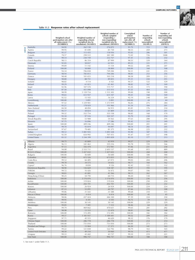
Table 11.5 Response rates after school replacement
Weighted school participation rate after
all replacement (%) (SCHRRW3)
Weighted number of responding schools (weighted also by
enrollment) (NUMW3)
Weighted number of schools sampled (responding +
non-responding) (weighted also by
enrollment) (DENW3)
Unweighted school
participation rate after all
replacement (%) (SCHRRU3)
Number of responding
schools (unweighted)
(NUMU3)
Number of responding and non-responding
schools (unweighted)
(DENU3)
OEC
D Australia 94.95 262 130 276 072 91.75 723 788Austria 99.95 81 690 81 730 98.53 269 273Belgium 95.37 113 435 118 936 95.02 286 301Canada 78.57 299 512 381 189 72.02 726 1008Chile 99.14 230 749 232 757 97.41 226 232Czech Republic 98.13 86 354 87 999 98.55 339 344Denmark 92.03 58 837 63 931 89.22 331 371Estonia 99.89 11 142 11 154 99.52 206 207Finland 100.00 58 800 58 800 100.00 168 168France 94.34 706 838 749 284 94.51 241 255Germany 98.94 785 813 794 206 98.83 253 256Greece 98.48 101 653 103 218 98.58 209 212Hungary 98.80 88 751 89 825 97.21 244 251Iceland 98.82 4 114 4 163 94.57 122 129Ireland 99.29 61 023 61 461 98.82 167 169Israel 92.96 107 570 115 717 91.05 173 190Italy 87.50 451 098 515 515 87.22 464 532Japan 98.99 1 139 734 1 151 305 99.00 198 200Korea 99.65 612 937 615 107 99.41 168 169Latvia 92.52 15 103 16 324 92.19 248 269Luxembourg 100.00 5 891 5 891 100.00 44 44Mexico 97.52 1 339 901 1 373 919 96.83 275 284Netherlands 93.21 178 929 191 966 91.54 184 201New Zealand 84.50 48 094 56 913 83.81 176 210Norway 95.17 58 824 61 809 95.02 229 241Poland 99.32 352 754 355 158 98.82 168 170Portugal 95.10 97 516 102 537 93.70 238 254Slovak Republic 98.80 53 908 54 562 97.63 288 295Slovenia 97.75 16 896 17 286 95.42 333 349Spain 100.00 409 246 409 246 100.00 201 201Sweden 99.70 93 819 94 097 98.54 202 205Switzerland 97.67 79 481 81 375 96.98 225 232Turkey 99.12 1 081 935 1 091 528 95.90 187 195United Kingdom 92.59 654 992 707 415 91.47 547 598United States 83.32 3 244 399 3 893 828 83.10 177 213
Part
ners Albania 99.75 43 809 43 919 99.57 229 230
Algeria 96.13 341 463 355 216 95.78 159 166Argentina 97.13 556 478 572 941 97.06 231 238Brazil 94.08 2 533 711 2 693 137 91.68 815 889B-S-J-G (China) 100.00 1 437 652 1 437 652 100.00 268 268Bulgaria 100.00 56 600 56 600 100.00 180 180Colombia 99.81 672 526 673 835 98.93 371 375Costa Rica 99.12 66 485 67 073 99.03 204 206Croatia 99.78 34 575 34 652 98.77 160 162Cyprus1 96.76 8 830 9 126 92.42 122 132Dominican Republic 98.90 136 669 138 187 98.97 193 195FYROM 99.72 16 426 16 472 99.07 106 107Georgia 98.83 41 081 41 566 98.13 262 267Hong Kong (China) 90.25 54 795 60 715 90.20 138 153Indonesia 100.00 3 176 076 3 176 076 100.00 236 236Jordan 100.00 119 024 119 024 100.00 250 250Kazakhastan 100.00 202 701 202 701 100.00 232 232Kosovo 100.00 26 924 26 924 100.00 224 224Lebanon 87.33 53 091 60 797 87.66 270 308Lithuania 99.86 31 543 31 588 99.68 310 311Macao (China) 100.00 4 414 4 414 100.00 45 45Malaysia 98.06 437 424 446 100 97.39 224 230Malta 99.95 4 341 4 343 96.72 59 61Moldova 100.00 30 145 30 145 100.00 229 229Montenegro 99.85 7 301 7 312 98.46 64 65Peru 99.79 469 662 470 651 99.65 281 282Qatar 98.98 13 333 13 470 98.81 166 168Romania 100.00 172 495 172 495 100.00 182 182Russia 99.37 1 181 937 1 189 441 99.52 209 210Singapore 97.71 45 553 46 620 98.32 176 179Chinese Taipei 100.00 286 778 286 778 100.00 214 214Thailand 100.00 751 010 751 010 100.00 273 273Trinidad and Tobago 91.55 15 904 17 371 86.50 141 163Tunisia 99.22 121 838 122 792 98.79 163 165United Arab Emirates 98.50 49 310 50 060 99.16 473 477Uruguay 99.33 43 442 43 737 99.10 219 221Viet Nam 100.00 996 757 996 757 100.00 188 188
1. See note 1 under Table 11.1.

11SAMPLING OUTCOMES
212 © OECD 2017 PISA 2015 TECHNICAL REPORT
Table 11.6 Response rates after school replacement, by adjudicated regions
Weighted school participation rate after all
replacement (%) (SCHRRW3)
Weighted number of responding
schools (weighted also by enrollment)
(NUMW3)
Weighted number of schools sampled
(responding + non-responding) (weighted also by enrollment)
(DENW3)
Unweighted school
participation rate after all
replacement (%) (SCHRRU3)
Number of responding
schools (unweighted)
(NUMU3)
Number of responding and non-responding
schools (unweighted)
(DENU3)
OEC
D Belgium (Flemish community) 93.45 61 039.32 65 319.22 93.55 174 186Spain (Andalusia) 100.00 82 192.73 82 192.73 100.00 54 54Spain (Aragon) 100.00 11 125.90 11 125.90 100.00 53 53Spain (Asturias) 100.00 7 065.53 7 065.53 100.00 54 54Spain (Balearic Islands) 100.00 9 501.65 9 501.65 100.00 54 54Spain (Basque Country) 100.00 18 113.27 18 113.27 100.00 119 119Spain (Canary Islands) 98.26 19 877.44 20 229.40 98.15 53 54Spain (Cantabria) 100.00 4 779.92 4 779.92 100.00 56 56Spain (Castile and Leon) 100.00 19 601.83 19 601.83 100.00 57 57Spain (CastileLaMancha) 100.00 19 542.72 19 542.72 100.00 55 55Spain (Catalonia) 100.00 67 606.13 67 606.13 100.00 52 52Spain (Extremadura) 100.00 10 592.13 10 592.13 100.00 53 53Spain (Galicia) 100.00 19 616.86 19 616.86 100.00 59 59Spain (La Rioja) 100.00 2 822.00 2 822.00 100.00 47 47Spain (Madrid) 100.00 53 137.04 53 137.04 100.00 51 51Spain (Murcia) 100.00 14 015.27 14 015.27 100.00 53 53Spain (Navarra) 100.00 5 793.20 5 793.20 100.00 52 52Spain (Valencia) 97.94 42 313.15 43 203.77 98.11 52 53United Kingdom (Scotland) 92.68 51 235.75 55 282.20 92.31 108 117United States (Massachusetts (public)) 91.85 64 205.61 69 899.08 90.57 48 53United States (North Carolina (public)) 100.00 110 785.88 110 785.88 100.00 54 54United States (Puerto Rico)1 100.00 39 453.16 39 453.16 100.00 47 47
Part
ners Argentina (CABA) 96.49 34 325.94 35 576.10 96.61 57 59
United Arab Emirates (Abu Dhabi) 96.14 18 652.63 19 402.38 96.55 112 116
United Arab Emirates (Dubai) 100.00 14 057.00 14 057.00 100.00 214 214
1. Puerto Rico is an unincorporated territory of the United States. As such, PISA results for the United States do not include Puerto Rico.
The weighted school response rate, after replacement, is given by the formula:
11.2
weighted school response rate
after replacement
WE
WE
i ii ∈ (Y∪R)
i
=ii
i ∈ (Y∪R∪N)
where Y denotes the set of responding original sample schools, R denotes the set of responding replacement schools, for which the corresponding original sample school was eligible but was non-responding, N denotes the set of eligible refusing original sample schools, Wi denotes the base weight for school i, Wi = 1/Pi, where Pi denotes the school selection probability for school i, and for weighted rates, Ei denotes the enrolment size of age-eligible students, as indicated on the sampling frame.
For unweighted student response rates, the numerator is the number of students for whom assessment data were included in the results less those in schools with between 25 and 50% student participation. The denominator is the number of sampled students who were age-eligible, and not explicitly excluded as student exclusions.
For weighted student response rates, the same number of students appears in the numerator and denominator as for unweighted rates, but each student was weighted by its student base weight. This is given as the product of the school base weight – for the school in which the student was enrolled – and the reciprocal of the student selection probability within the school.
In countries with no oversampling of any explicit strata, weighted and unweighted student participation rates are very similar.
Overall response rates are calculated as the product of school and student response rates. Although overall weighted and unweighted rates can be calculated, there is little value in presenting overall unweighted rates. The weighted rates indicate the proportion of the student population represented by the sample prior to making the school and student non-response adjustments.

11SAMPLING OUTCOMES
PISA 2015 TECHNICAL REPORT © OECD 2017 213
Table 11.7 Response rates, students within schools after school replacement
Weighted student participation rate
after second replacement (%)
(STURRW3)
Number of students assessed
(Weighted) (NUMSTW3)
Number of students sampled
(assessed + absent) (weighted) DENSTW3)
Unweighted student
participation rate after second replacement (%)
(STURRU3)
Number of students
assessed (unweighted) (NUMSTU3)
Number of students sampled
(assessed + absent) (unweighted) (DENSTU3)
OEC
D Australia 83.99 204 763 243 789 80.61 14 089 17 477Austria 86.59 63 660 73 521 71.01 7 007 9 868Belgium 90.63 99 760 110 075 90.88 9 635 10 602Canada 80.80 210 476 260 487 81.25 19 604 24 129Chile 93.31 189 206 202 774 93.67 7 039 7 515Czech Republic 88.77 73 386 82 672 88.85 6 835 7 693Denmark 89.08 49 732 55 830 87.35 7 149 8 184Estonia 93.22 10 088 10 822 93.21 5 587 5 994Finland 93.44 53 198 56 934 93.45 5 882 6 294France 88.21 611 563 693 336 88.16 5 980 6 783Germany 93.27 685 972 735 487 93.26 6 476 6 944Greece 94.32 89 588 94 986 94.40 5 511 5 838Hungary 92.30 77 212 83 657 92.49 5 643 6 101Iceland 86.11 3 365 3 908 86.11 3 365 3 908Ireland 88.60 51 947 58 630 88.62 5 741 6 478Israel 90.48 98 572 108 940 90.46 6 598 7 294Italy 87.67 377 011 430 041 89.38 11 477 12 841Japan 97.24 1 096 193 1 127 265 97.21 6 647 6 838Korea 98.56 559 121 567 284 98.53 5 581 5 664Latvia 90.42 12 799 14 155 90.26 4 845 5 368Luxembourg 95.65 5 299 5 540 95.65 5 299 5 540Mexico 95.43 1 290 435 1 352 237 95.34 7 568 7 938Netherlands 85.12 152 346 178 985 85.26 5 345 6 269New Zealand 80.31 36 860 45 897 80.28 4 453 5 547Norway 90.75 50 163 55 277 90.69 5 456 6 016Poland 87.54 300 617 343 405 87.43 4 466 5 108Portugal 82.02 75 391 91 916 82.23 7 180 8 732Slovak Republic 92.37 45 357 49 103 91.91 6 342 6 900Slovenia 91.77 15 072 16 424 91.40 6 406 7 009Spain 89.14 356 509 399 935 89.34 6 736 7 540Sweden 90.67 82 582 91 081 90.77 5 458 6 013Switzerland 92.45 74 465 80 544 92.59 5 838 6 305Turkey 95.19 874 609 918 816 94.91 5 895 6 211United Kingdom 89.02 517 426 581 252 87.58 14 120 16 123United States 89.76 2 629 707 2 929 771 89.59 5 712 6 376
Part
ners Albania 93.53 38 174 40 814 93.84 5 213 5 555
Algeria 92.47 274 121 296 434 92.59 5 494 5 934Argentina 90.36 345 508 382 352 89.95 6 311 7 016Brazil 87.32 1 996 574 2 286 505 85.73 22 791 26 586B-S-J-G (China) 96.69 1 287 710 1 331 794 97.46 9 841 10 097Bulgaria 94.87 50 931 53 685 95.00 5 928 6 240Colombia 94.52 535 682 566 734 93.39 11 777 12 611Costa Rica 92.46 47 494 51 369 92.38 6 846 7 411Croatia 91.35 37 275 40 803 91.42 5 809 6 354Cyprus* 94.03 8 016 8 526 93.35 5 561 5 957Dominican Republic 93.82 122 620 130 700 94.13 4 731 5 026FYROM 94.92 14 999 15 802 94.78 5 324 5 617Georgia 93.91 35 567 37 873 93.44 5 316 5 689Hong Kong (China) 93.08 48 222 51 806 93.25 5 359 5 747Indonesia 97.51 3 015 844 3 092 773 97.30 6 513 6 694Jordan 97.42 105 868 108 669 97.39 7 267 7 462Kazakhastan 97.29 187 683 192 921 97.29 7 841 8 059Kosovo 98.58 22 016 22 333 98.57 4 826 4 896Lebanon 94.52 36 052 38 143 94.95 4 546 4 788Lithuania 90.57 27 070 29 889 90.57 6 523 7 202Macao (China) 99.31 4 476 4 507 99.31 4 476 4 507Malaysia 96.66 393 785 407 396 97.21 8 843 9 097Malta 84.63 3 634 4 294 84.63 3 634 4 294Moldova 98.00 28 754 29 341 97.96 5 325 5 436Montenegro 93.79 6 346 6 766 93.74 5 665 6 043Peru 98.90 426 205 430 959 98.82 6 971 7 054Qatar 94.09 12 061 12 819 94.09 12 061 12 819Romania 99.21 162 918 164 216 99.31 4 876 4 910Russia 96.83 1 072 914 1 108 068 96.88 6 021 6 215Singapore 93.33 42 241 45 259 93.14 6 105 6 555Chinese Taipei 98.00 246 408 251 424 97.93 7 708 7 871Thailand 96.88 614 996 634 795 97.15 8 249 8 491Trinidad and Tobago 79.38 9 674 12 188 79.84 4 587 5 745Tunisia 86.40 97 337 112 665 86.48 5 340 6 175United Arab Emirates 94.62 43 774 46 263 94.36 14 167 15 014Uruguay 86.16 32 762 38 023 86.24 6 059 7 026Viet Nam 99.60 871 353 874 859 99.61 5 826 5 849
* See note 1 under Table 11.1.

11SAMPLING OUTCOMES
214 © OECD 2017 PISA 2015 TECHNICAL REPORT
Table 11.8 Response rates, students within schools after school replacement, by adjudicated regions
Weighted student participation
rate after second replacement (%)
(STURRW3)
Number of students assessed
(weighted) (NUMSTW3)
Number of students sampled
(assessed + absent) (weighted)
(DENSTW3)
Unweighted student participation
rate after second replacement (%)
(STURRU3)
Number of students assessed
(Unweighted) (NUMSTU3)
Number of students sampled
(assessed + absent)
(unweighted) (DENSTU3)
OEC
D Belgium (Flemish community) 91.54 54 082.90 59 081.47 91.53 5 674 6 199Spain (Andalusia) 87.64 71 549.56 81 642.36 87.80 1 813 2 065Spain (Aragon) 89.49 9 626.75 10 757.56 89.54 1 798 2 008Spain (Asturias) 89.63 6 179.65 6 894.55 89.72 1 790 1 995Spain (Balearic Islands) 88.84 8 179.56 9 207.58 88.92 1 797 2 021Spain (Basque Country) 91.07 15 868.19 17 424.20 90.48 3 612 3 992Spain (Canary Islands) 90.40 17 279.43 19 113.67 90.39 1 825 2 019Spain (Cantabria) 90.39 4 136.09 4 575.66 90.58 1 924 2 124Spain (Castile and Leon) 92.03 16 568.49 18 003.77 91.98 1 858 2 020Spain (CastileLaMancha) 90.24 17 368.92 19 247.29 90.30 1 889 2 092Spain (Catalonia) 90.66 57 218.40 63 112.16 90.72 1 769 1 950Spain (Extremadura) 89.90 9 038.97 10 054.22 89.91 1 809 2 012Spain (Galicia) 91.13 17 371.25 19 062.58 91.06 1 865 2 048Spain (La Rioja) 91.71 2 529.21 2 757.90 91.89 1 461 1 590Spain (Madrid) 89.77 47 792.04 53 239.55 90.00 1 808 2 009Spain (Murcia) 86.96 11 787.15 13 555.12 87.02 1 796 2 064Spain (Navarra) 94.02 5 166.61 5 495.51 94.17 1 874 1 990Spain (Valencia) 87.50 33 270.94 38 024.57 87.55 1 611 1 840United Kingdom (Scotland) 79.99 37 114.07 46 396.20 79.99 3 095 3 869United States (Massachusetts (public)) 90.36 42 557.08 47 096.94 90.68 1 391 1 534United States (North Carolina (public)) 92.43 96 277.78 104 161.17 92.59 1 887 2 038United States (Puerto Rico)1 93.12 28 179.19 30 261.01 93.64 1 398 1 493
Part
ners Argentina (CABA) 90.34 28 282.38 31 306.97 89.33 1 649 1 846
United Arab Emirates (Abu Dhabi) 93.40 16 483.27 17 647.64 93.09 3 610 3 878
United Arab Emirates (Dubai) 94.34 12 174.95 12 905.86 94.16 6 287 6 677
1. Puerto Rico is an unincorporated territory of the United States. As such, PISA results for the United States do not include Puerto Rico.
Table 11.9 Science teacher response rates
CountryScience teacher
unweighted response rate (%) Science teacher numerator Science teacher denominatorNumber of ineligible
science teachers
OEC
D Australia 73.49 4 158 5 658 72Chile 90.07 771 856 110Czech Republic 94.88 2 169 2 286 18Germany 68.90 2 032 2 949 0Italy 74.50 2 422 3 251 23Korea 99.36 926 932 4Portugal 91.20 1 441 1 580 29Spain 95.53 1 368 1 432 33United States 87.20 1 110 1 273 12United States (Massachusetts (public)) 90.49 390 431 9United States (North Carolina (public)) 97.19 380 391 2
Part
ners Brazil 70.35 2 650 3 767 0
B-S-J-G (China) 99.30 2 410 2 427 29
Colombia 85.42 1 324 1 550 57
Dominican Republic 91.13 452 496 33
Hong Kong (China) 91.48 1 042 1 139 4
Macao (China) 98.99 391 395 2
Malaysia 97.67 2 010 2 058 41
Peru 95.65 902 943 33
Chinese Taipei 98.98 1 545 1 561 9
United Arab Emirates 89.13 1 795 2 014 10
United Arab Emirates (Abu Dhabi) 87.83 729 830 7
United Arab Emirates (Dubai) 90.34 1 103 1 221 7
TEACHER RESPONSE RATESUnweighted response rates for both science and non-science teachers were created using similar methods to those for unweighted student and school response rates – that is, ineligible teachers are not used in the denominator for the rate calculation.
These rates are presented in Table 11.9 for science teachers and in Table 11.10 for the non-science teachers.
In addition to these rates, unweighted response rates were calculated also for each sampled school in each country which implemented the Teacher Questionnaire. These rates were created as quality indicators for the questionnaire team who would use the Teacher Questionnaire data to create derived variables to help provide context about PISA students.

11SAMPLING OUTCOMES
PISA 2015 TECHNICAL REPORT © OECD 2017 215
Table 11.10 Non-science teacher response rates
CountryNon-Science teacher
unweighted response rate (%)Non-Science teacher
numeratorNon-Science teacher
denominatorNumber of ineligible non-science teachers
OEC
D Australia 71.25 7 394 10 378 126
Chile 90.68 2 295 2 531 100
Czech Republic 93.75 3 750 4 000 55
Germany 64.90 3 568 5 498 0
Italy 70.45 4 526 6 424 52
Korea 99.12 2 128 2 147 20
Portugal 88.20 2 257 2 559 60
Spain 92.46 2 526 2 732 89
United States 88.53 2 099 2 371 24
United States (Massachusetts (public)) 89.36 630 705 10
United States (North Carolina (public)) 95.47 738 773 14
Part
ners Brazil 67.01 5 398 8 055 0
B-S-J-G (China) 99.03 3 880 3 918 49
Colombia 82.89 3 295 3 975 90
Dominican Republic 86.97 1 048 1 205 93
Hong Kong (China) 89.80 1 841 2 050 5
Macao (China) 99.34 2 410 2 426 4
Malaysia 97.44 3 191 3 275 85
Peru 99.32 2 918 2 938 123
Chinese Taipei 99.08 3 130 3 159 17
United Arab Emirates 87.23 3 285 3 766 30
United Arab Emirates (Abu Dhabi) 87.29 1 222 1 400 11
United Arab Emirates (Dubai) 88.78 2 026 2 282 25
DESIGN EFFECTS AND EFFECTIVE SAMPLE SIZESSurveys in education and especially international surveys rarely sample students by simply selecting a random sample of students (known as a simple random sample, or SRS). Rather, a sampling design is used where schools are first selected and, within each selected school, classes or students are randomly sampled. Sometimes, geographic areas are first selected before sampling schools and students. This sampling design is usually referred to as a cluster sample or a multi-stage sample.
Selected students attending the same school cannot be considered as independent observations as assumed with a simple random sample because they are usually more similar to one another than to students attending other schools. For instance, the students are offered the same school resources, may have the same teachers and therefore are taught a common implemented curriculum, and so on. School differences are also larger if different educational programmes are not available in all schools. One expects to observe greater differences between a vocational school and an academic school than between two comprehensive schools.
Furthermore, it is well known that within a country, within sub-national entities and within a city, people tend to live in areas according to their financial resources. As children usually attend schools close to their home, it is likely that students attending the same school come from similar social and economic backgrounds.
A simple random sample of 4 000 students is thus likely to cover the diversity of the population better than a sample of 100 schools with 40 students observed within each school. It follows that the uncertainty associated with any population parameter estimate (i.e., standard error) will be larger for a clustered sample estimate than for a simple random sample estimate of the same size.
In the case of a simple random sample, the standard error of a mean estimate is equal to:
11.3
σσ
μ( ) =2
nˆ
where σ2 denotes the variance of the whole student population and n is the student sample size.
11SAMPLING OUTCOMES
216 © OECD 2017 PISA 2015 TECHNICAL REPORT
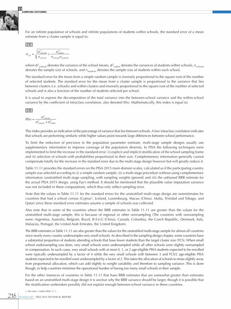
For an infinite population of schools and infinite populations of students within schools, the standard error of a mean estimate from a cluster sample is equal to:
11.4
σσ σ
μ( ) = +schools
schools
within
schools studentsn n n
2 2
ˆ
where σ2schools denotes the variance of the school means, σ2
within denotes the variances of students within schools, nschools denotes the sample size of schools, and nstudents denotes the sample size of students within each school.
The standard error for the mean from a simple random sample is inversely proportional to the square root of the number of selected students. The standard error for the mean from a cluster sample is proportional to the variance that lies between clusters (i.e. schools) and within clusters and inversely proportional to the square root of the number of selected schools and is also a function of the number of students selected per school.
It is usual to express the decomposition of the total variance into the between-school variance and the within-school variance by the coefficient of intraclass correlation, also denoted Rho. Mathematically, this index is equal to:
11.5
Rho schools
schools within
=+
σσ σ
2
2 2
This index provides an indication of the percentage of variance that lies between schools. A low intraclass correlation indicates that schools are performing similarly while higher values point towards large differences between school performance.
To limit the reduction of precision in the population parameter estimate, multi-stage sample designs usually use supplementary information to improve coverage of the population diversity. In PISA the following techniques were implemented to limit the increase in the standard error: (i) explicit and implicit stratification of the school sampling frame and (ii) selection of schools with probabilities proportional to their size. Complementary information generally cannot compensate totally for the increase in the standard error due to the multi-stage design however but will greatly reduce it.
Table 11.11 provides the standard errors on the PISA 2015 main domain scales, calculated as if the participating country sample was selected according to (i) a simple random sample; (ii) a multi-stage procedure without using complementary information (unstratified multi-stage sampling, with sampling weights ignored) and (iii) the unbiased BRR estimate for the actual PISA 2015 design, using Fay’s method. It should be mentioned that the plausible value imputation variance was not included in these computations, which thus only reflect sampling error.
Note that the values in Table 11.11 for the standard errors for the unstratified multi-stage design are overestimates for countries that had a school census (Cyprus1, Iceland, Luxembourg, Macao (China), Malta, Trinidad and Tobago, and Qatar) since these standard error estimates assume a sample of schools was collected.
Also note that in some of the countries where the BRR estimates in Table 11.11 are greater than the values for the unstratified multi-stage sample, this is because of regional or other oversampling (The countries with oversampling were: Argentina, Australia, Belgium, Brazil, B-S-J-G (China), Canada, Colombia, the Czech Republic, Denmark, Italy, Malaysia, Portugal, the United Arab Emirates, the United Kingdom).
The BRR estimates in Table 11.11 are also greater than the values for the unstratified multi-stage sample for almost all countries since nearly every country undersamples very small schools. As described in the sampling design chapter, some countries have a substantial proportion of students attending schools that have fewer students than the target cluster size (TCS). When small school undersampling was done, very small schools were undersampled while all other schools were slightly oversampled in compensation. In such cases, very small schools with at most 0, 1, or 2 age-eligible PISA students expected to be enrolled were typically undersampled by a factor of 4 while the very small schools with between 3 and TCS/2 age-eligible PISA students expected to be enrolled were undersampled by a factor of 2. This takes the allocation of schools to strata slightly away from proportional allocation, which can add slightly to weight variability and therefore to sampling variance. This is done though, to help countries minimise the operational burden of having too many small schools in their sample.
For the other instances of countries in Table 11.11 that have BRR estimates that are somewhat greater than estimates based on an unstratified multi-stage design it is unclear why the BRR variance should be larger, though it is possible that the stratification undertaken possibly did not explain enough between-school variance in these countries.
1. See note 1 under Table 11.1.

11SAMPLING OUTCOMES
PISA 2015 TECHNICAL REPORT © OECD 2017 217
It is usual to express the effect of the sampling design on the standard errors by a statistic referred to as the design effect. This corresponds to the ratio of the variance of the estimate obtained from the (more complex) sample to the variance of the estimate that would be obtained from a simple random sample of the same number of sampling units. The design effect has two primary uses – in sample size estimation and in appraising the efficiency of more complex sampling plans (Cochran, 1977).
In PISA, as sampling variance has to be estimated by using the 80 BRR replicates, a design effect can be computed for a statistic t using:
11.6
Deff tVar tVar t
BRR
SRS
( )( )( )
=
where VarBRR(t) is the sampling variance for the statistic t computed by the BRR replication method, and VarSRS(t) is the sampling variance for the same statistic t on the same data but considering the sample as a simple random sample.
Based on Table 11.11, the unbiased BRR standard error on the mean estimate in science in Australia (for example) is equal to 1.46 (rounded from 1.45568). As the standard deviation of the science performance is equal to 102.29735, the design effect in Australia for the mean estimate in science is therefore equal to:
11.7
Deff tVar tVar t
BRR
SRS
( )( )( )
(1.45568)2
= =⎡⎣ ⎤⎦
= 2.942195102.297352/14 530
The sampling variance on the science performance mean in Australia is about 2.94 times larger than it would have been with a simple random sample of the same sample size. Note that the participating students are 14 530 as this number were assessed for science.
Another way to express the reduction of precision due to the complex sampling design is through the effective sample size, which expresses the simple random sample size that would give the same sampling variance as the one obtained from the actual complex sample design. The effective sample size for a statistic t is equal to:
11.8
Effn tn
Deff t
n × VarSRS(t)
VarBRR(t)( )
( )= =
where n is equal to the actual number of units in the sample. The effective sample size in Australia for the science performance mean is equal to:
11.9
Effn tn
Deff t( )
( )= = =
14 5302.942195
4938.4898
In other words, a simple random sample of 4 938 students in Australia would have been as precise as the actual PISA 2015 sample for the national estimate of mean science proficiency.
VARIABILITY OF THE DESIGN EFFECTNeither the design effect nor the effective sample size is a definitive characteristic of a sample. Both the design effect and the effective sample size vary with the variable and statistic of interest.
As previously stated, the sampling variance for estimates of the mean from a cluster sample is proportional to the intraclass correlation. In some countries, student performance varies between schools. Students in academic schools usually tend to perform well while on average student performance in vocational schools is lower. Let us now suppose that the height of the students was also measured, and there are no reasons why students in academic schools should be of different height than students in vocational schools. For this particular variable, the expected value of the between-school variance should be equal to zero and therefore, the design effect should tend to one. As the segregation effect differs according to the variable, the design effect will also differ according to the variable.
The second factor that influences the size of the design effect is the choice of requested statistics. It tends to be large for means, proportions, and sums but substantially smaller for bivariate or multivariate statistics such as correlation and regression coefficients.
11SAMPLING OUTCOMES
218 © OECD 2017 PISA 2015 TECHNICAL REPORT
Design effects in PISA for performance variablesThe notion of design effect as given earlier is extended and gives rise to five different design effect formulae to describe the influence of the sampling and test designs on the standard errors for statistics.
The total errors computed for the international PISA initial reports (OECD, 2016a,b) that involves performance variables (scale scores) consist of two components: sampling variance and measurement variance. The standard error of proficiency estimates in PISA is inflated because the students were not sampled according to a simple random sample and also because the estimation of student proficiency includes some amount of measurement error.
For any statistic r, the population estimate and the sampling variance are computed for each plausible value and then combined as described in Chapter 9.
The five design effects and their respective effective sample sizes are defined as follows:
• Design Effect 1
11.10
Deff rVar r MVar r
Var rSRS
SRS1( )
( ) ( )( )
=+
where MVar(r) is the measurement variance for the statistic r. This design effect shows the inflation of the total variance that would have occurred due to measurement error if in fact the samples were considered as a simple random sample.
• Design Effect 2
11.11
Deff rVar r MVar rVar r MVar r
BRR
SRS2( )
( ) ( )( ) ( )
=++
shows the inflation of the total variance due only to the use of a complex sampling design.
• Design Effect 3
11.12
Deff rVar rVar r
BRR
SRS3( )
( )( )
=
shows the inflation of the sampling variance due to the use of a complex design.
• Design Effect 4
11.13
Deff rVar r MVar r
Var rBRR
BRR4( )
( ) ( )( )
=+
shows the inflation of the total variance due to measurement variance.
• Design Effect 5
11.14
Deff rVar r MVar r
Var rBRR
SRS5( )
( ) ( )( )
=+
shows the inflation of the total variance due to the measurement variance and due to the complex sampling design.
The product of the first and second design effects equals the product of the third and fourth design effects, and both products are equal to the fifth design effect.
Tables 11.12 through 11.16 present the values of the different design effects and the corresponding effective sample sizes for each of the major domains.

11SAMPLING OUTCOMES
PISA 2015 TECHNICAL REPORT © OECD 2017 219
Table 11.11 Standard errors for the PISA 2015 main domain scales
Country
Collaborative problem solving Financial literacy Mathematical literacy Reading literacy Science literacy
Simple random sample
Unbiased BRR
Simple random sample
Unbiased BRR
Simple random sample
Unbiased BRR
Simple random sample
Unbiased BRR
Simple random sample
Unbiased BRR
OEC
D Australia 0.88 1.52 0.98 1.84 0.77 1.33 0.85 1.36 0.85 1.46Austria 1.18 2.34 1.14 2.68 1.21 2.57 1.16 2.40Belgium 1.00 2.24 1.41 2.61 0.99 2.27 1.02 2.34 1.02 2.27Canada 0.74 2.08 0.93 3.65 0.62 2.14 0.66 2.15 0.65 2.06Chile 1.00 2.28 1.20 2.97 1.02 2.36 1.05 2.51 1.02 2.33Czech Republic 1.10 1.99 1.09 2.23 1.21 2.48 1.15 2.25Denmark 1.07 2.34 0.95 2.01 1.03 2.41 1.07 2.35Estonia 1.21 2.02 1.08 1.78 1.17 2.01 1.19 1.96Finland 1.32 2.30 1.07 2.03 1.22 2.51 1.25 2.36France 1.28 1.93 1.22 1.98 1.43 2.36 1.30 2.03Germany 1.25 2.48 1.10 2.45 1.24 2.89 1.23 2.63Greece 1.24 3.47 1.20 3.56 1.32 4.27 1.24 3.89Hungary 1.27 2.25 1.25 2.35 1.29 2.49 1.28 2.38Iceland 1.63 1.72 1.60 1.68 1.71 1.80 1.57 1.66Ireland 1.05 2.00 1.14 2.27 1.17 2.29Israel 1.36 3.52 1.27 3.41 1.39 3.73 1.31 3.42Italy 0.89 2.42 0.85 2.42 0.87 2.63 0.87 2.43 0.85 2.46Japan 1.04 2.55 1.08 2.77 1.13 3.11 1.15 2.94Korea 1.12 2.23 1.33 3.49 1.30 3.25 1.27 3.09Latvia 1.29 1.74 1.11 1.54 1.21 1.64 1.18 1.46Luxembourg 1.37 1.07 1.29 0.82 1.46 0.96 1.38 0.86Mexico 0.91 2.21 0.86 2.21 0.90 2.37 0.82 2.06Netherlands 1.32 2.24 1.53 2.51 1.25 2.08 1.38 2.22 1.38 2.22New Zealand 1.57 2.19 1.37 2.11 1.56 2.26 1.55 2.35Norway 1.27 2.22 1.15 2.05 1.34 2.34 1.30 2.23Poland 1.48 2.70 1.31 2.31 1.34 2.26 1.36 2.48Portugal 1.07 2.38 1.12 2.41 1.07 2.47 1.07 2.35Puerto Rico (United States)1 2.06 5.35 2.56 6.94 2.31 6.00Slovak Republic 1.17 2.27 1.44 3.38 1.20 2.47 1.31 2.71 1.24 2.56Slovenia 1.16 1.34 1.10 1.14 1.15 1.16 1.19 1.23Spain 1.07 1.96 1.21 2.74 1.03 2.02 1.06 2.18 1.07 2.05Sweden 1.33 3.22 1.22 3.06 1.38 3.40 1.39 3.53Switzerland 1.25 2.80 1.28 2.89 1.30 2.86Turkey 1.02 3.38 1.07 4.08 1.07 3.91 1.03 3.88United Kingdom 0.87 2.47 0.78 2.42 0.81 2.51 0.84 2.47United States 1.43 3.44 1.35 3.49 1.17 3.07 1.32 3.32 1.30 3.13
Part
ners Albania 1.19 3.37 1.34 4.00 1.09 3.20
Algeria 0.96 2.83 0.98 2.84 0.93 2.56Argentina 1.01 3.00 1.11 3.17 1.01 2.75Brazil 0.58 2.11 0.72 3.17 0.59 2.55 0.66 2.44 0.59 2.27B-S-J-G (China) 0.98 3.90 1.18 5.40 1.07 4.74 1.10 5.08 1.04 4.62Bulgaria 1.27 3.79 1.26 3.88 1.49 4.87 1.32 4.34Colombia 0.76 2.27 0.71 2.15 0.83 2.79 0.74 2.31Costa Rica 0.94 2.17 0.83 2.12 0.96 2.57 0.85 2.04Croatia 1.14 2.36 1.16 2.56 1.19 2.59 1.17 2.42Cyprus2 1.22 1.25 1.24 1.13 1.37 1.32 1.24 1.22Dominican Republic 1.00 2.29 1.23 2.94 1.05 2.45FYROM 1.31 1.16 1.36 1.17 1.16 1.08Georgia 1.29 2.61 1.42 2.76 1.24 2.36Hong Kong (China) 1.24 2.75 1.23 2.87 1.17 2.59 1.10 2.43Indonesia 0.99 2.91 0.94 2.72 0.85 2.49Jordan 1.01 2.45 1.10 2.71 0.99 2.62Kazakhstan 0.93 3.90 0.91 3.11 0.86 3.61Kosovo 1.08 1.47 1.13 1.42 1.03 1.37Lebanon 1.50 3.57 1.71 4.22 1.34 3.31Lithuania 1.12 2.31 1.19 2.77 1.07 2.23 1.17 2.68 1.13 2.57Macao (China) 1.34 0.96 1.19 0.89 1.23 0.87 1.22 0.90Malaysia 0.85 3.22 0.85 3.11 0.86 3.37 0.80 2.95Malta 1.83 1.43 2.00 1.54 1.95 1.45Moldova 1.24 2.25 1.34 2.41 1.18 1.90Montenegro 1.05 0.94 1.15 1.02 1.25 1.10 1.13 0.98Peru 1.00 2.38 1.23 3.07 0.99 2.43 1.07 2.76 0.92 2.30Qatar 0.90 0.67 1.01 0.77 0.90 0.71Romania 1.24 3.70 1.36 3.99 1.13 3.21Russia 1.19 3.28 1.11 3.07 1.07 2.99 1.13 2.94 1.06 2.90Singapore 1.24 1.07 1.22 1.15 1.26 1.23 1.32 1.11Chinese Taipei 1.03 2.29 1.17 2.68 1.06 2.42 1.13 2.62Thailand 0.92 3.35 0.90 2.94 0.88 3.21 0.86 2.79Trinidad and Tobago 1.40 1.05 1.52 1.24 1.37 1.12Tunisia 0.80 1.84 1.15 2.84 1.11 2.61 0.88 2.01United Arab Emirates 0.80 2.28 0.81 2.20 0.89 2.67 0.83 2.40Uruguay 1.17 2.17 1.11 2.16 1.24 2.42 1.11 2.17Viet Nam 1.10 4.38 0.95 3.67 1.00 3.86
1. Puerto Rico is an unincorporated territory of the United States. As such, PISA results for the United States do not include Puerto Rico. 2. See note 1 under Table 11.1.
11SAMPLING OUTCOMES
220 © OECD 2017 PISA 2015 TECHNICAL REPORT
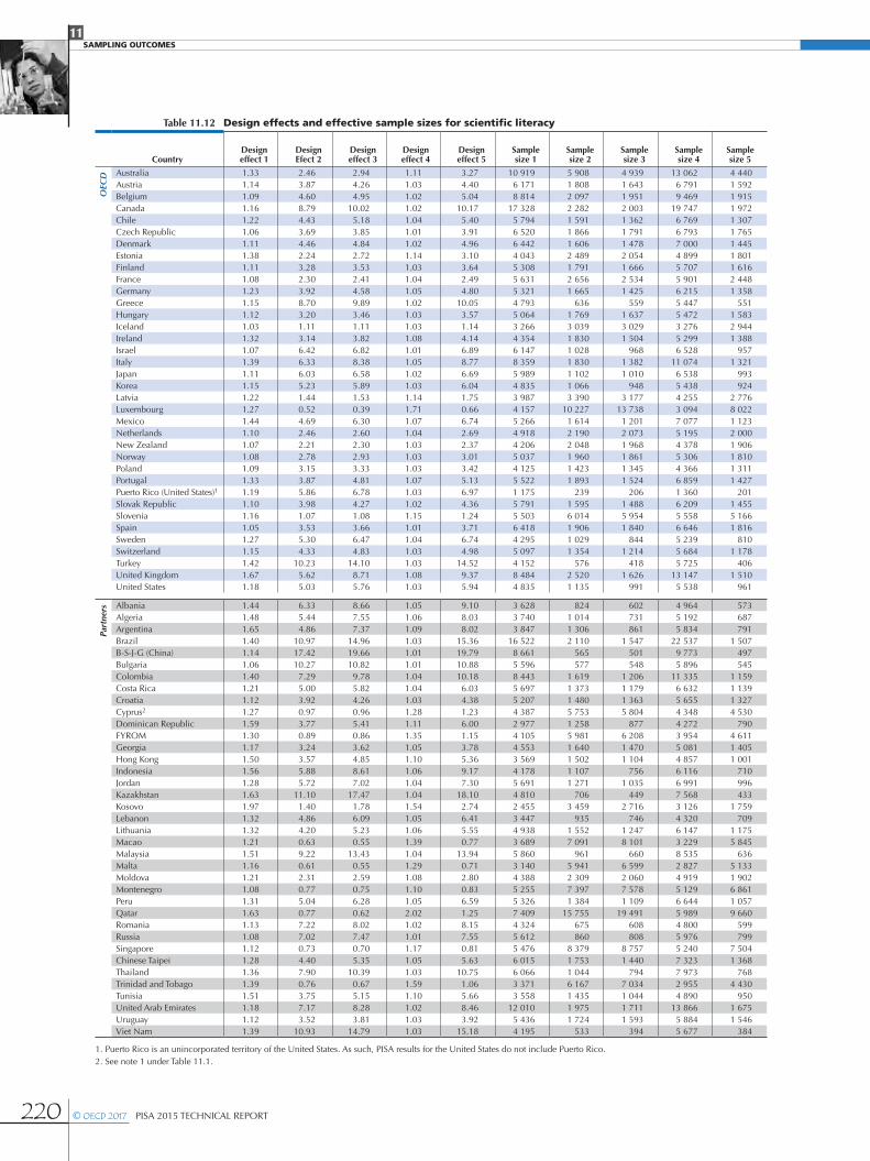
Table 11.12 Design effects and effective sample sizes for scientific literacy
CountryDesign effect 1
Design Efect 2
Design effect 3
Design effect 4
Design effect 5
Sample size 1
Sample size 2
Sample size 3
Sample size 4
Sample size 5
OEC
D Australia 1.33 2.46 2.94 1.11 3.27 10 919 5 908 4 939 13 062 4 440Austria 1.14 3.87 4.26 1.03 4.40 6 171 1 808 1 643 6 791 1 592Belgium 1.09 4.60 4.95 1.02 5.04 8 814 2 097 1 951 9 469 1 915Canada 1.16 8.79 10.02 1.02 10.17 17 328 2 282 2 003 19 747 1 972Chile 1.22 4.43 5.18 1.04 5.40 5 794 1 591 1 362 6 769 1 307Czech Republic 1.06 3.69 3.85 1.01 3.91 6 520 1 866 1 791 6 793 1 765Denmark 1.11 4.46 4.84 1.02 4.96 6 442 1 606 1 478 7 000 1 445Estonia 1.38 2.24 2.72 1.14 3.10 4 043 2 489 2 054 4 899 1 801Finland 1.11 3.28 3.53 1.03 3.64 5 308 1 791 1 666 5 707 1 616France 1.08 2.30 2.41 1.04 2.49 5 631 2 656 2 534 5 901 2 448Germany 1.23 3.92 4.58 1.05 4.80 5 321 1 665 1 425 6 215 1 358Greece 1.15 8.70 9.89 1.02 10.05 4 793 636 559 5 447 551Hungary 1.12 3.20 3.46 1.03 3.57 5 064 1 769 1 637 5 472 1 583Iceland 1.03 1.11 1.11 1.03 1.14 3 266 3 039 3 029 3 276 2 944Ireland 1.32 3.14 3.82 1.08 4.14 4 354 1 830 1 504 5 299 1 388Israel 1.07 6.42 6.82 1.01 6.89 6 147 1 028 968 6 528 957Italy 1.39 6.33 8.38 1.05 8.77 8 359 1 830 1 382 11 074 1 321Japan 1.11 6.03 6.58 1.02 6.69 5 989 1 102 1 010 6 538 993Korea 1.15 5.23 5.89 1.03 6.04 4 835 1 066 948 5 438 924Latvia 1.22 1.44 1.53 1.14 1.75 3 987 3 390 3 177 4 255 2 776Luxembourg 1.27 0.52 0.39 1.71 0.66 4 157 10 227 13 738 3 094 8 022Mexico 1.44 4.69 6.30 1.07 6.74 5 266 1 614 1 201 7 077 1 123Netherlands 1.10 2.46 2.60 1.04 2.69 4 918 2 190 2 073 5 195 2 000New Zealand 1.07 2.21 2.30 1.03 2.37 4 206 2 048 1 968 4 378 1 906Norway 1.08 2.78 2.93 1.03 3.01 5 037 1 960 1 861 5 306 1 810Poland 1.09 3.15 3.33 1.03 3.42 4 125 1 423 1 345 4 366 1 311Portugal 1.33 3.87 4.81 1.07 5.13 5 522 1 893 1 524 6 859 1 427Puerto Rico (United States)1 1.19 5.86 6.78 1.03 6.97 1 175 239 206 1 360 201Slovak Republic 1.10 3.98 4.27 1.02 4.36 5 791 1 595 1 488 6 209 1 455Slovenia 1.16 1.07 1.08 1.15 1.24 5 503 6 014 5 954 5 558 5 166Spain 1.05 3.53 3.66 1.01 3.71 6 418 1 906 1 840 6 646 1 816Sweden 1.27 5.30 6.47 1.04 6.74 4 295 1 029 844 5 239 810Switzerland 1.15 4.33 4.83 1.03 4.98 5 097 1 354 1 214 5 684 1 178Turkey 1.42 10.23 14.10 1.03 14.52 4 152 576 418 5 725 406United Kingdom 1.67 5.62 8.71 1.08 9.37 8 484 2 520 1 626 13 147 1 510United States 1.18 5.03 5.76 1.03 5.94 4 835 1 135 991 5 538 961
Part
ners Albania 1.44 6.33 8.66 1.05 9.10 3 628 824 602 4 964 573
Algeria 1.48 5.44 7.55 1.06 8.03 3 740 1 014 731 5 192 687Argentina 1.65 4.86 7.37 1.09 8.02 3 847 1 306 861 5 834 791Brazil 1.40 10.97 14.96 1.03 15.36 16 522 2 110 1 547 22 537 1 507B-S-J-G (China) 1.14 17.42 19.66 1.01 19.79 8 661 565 501 9 773 497Bulgaria 1.06 10.27 10.82 1.01 10.88 5 596 577 548 5 896 545Colombia 1.40 7.29 9.78 1.04 10.18 8 443 1 619 1 206 11 335 1 159Costa Rica 1.21 5.00 5.82 1.04 6.03 5 697 1 373 1 179 6 632 1 139Croatia 1.12 3.92 4.26 1.03 4.38 5 207 1 480 1 363 5 655 1 327Cyprus2 1.27 0.97 0.96 1.28 1.23 4 387 5 753 5 804 4 348 4 530Dominican Republic 1.59 3.77 5.41 1.11 6.00 2 977 1 258 877 4 272 790FYROM 1.30 0.89 0.86 1.35 1.15 4 105 5 981 6 208 3 954 4 611Georgia 1.17 3.24 3.62 1.05 3.78 4 553 1 640 1 470 5 081 1 405Hong Kong 1.50 3.57 4.85 1.10 5.36 3 569 1 502 1 104 4 857 1 001Indonesia 1.56 5.88 8.61 1.06 9.17 4 178 1 107 756 6 116 710Jordan 1.28 5.72 7.02 1.04 7.30 5 691 1 271 1 035 6 991 996Kazakhstan 1.63 11.10 17.47 1.04 18.10 4 810 706 449 7 568 433Kosovo 1.97 1.40 1.78 1.54 2.74 2 455 3 459 2 716 3 126 1 759Lebanon 1.32 4.86 6.09 1.05 6.41 3 447 935 746 4 320 709Lithuania 1.32 4.20 5.23 1.06 5.55 4 938 1 552 1 247 6 147 1 175Macao 1.21 0.63 0.55 1.39 0.77 3 689 7 091 8 101 3 229 5 845Malaysia 1.51 9.22 13.43 1.04 13.94 5 860 961 660 8 535 636Malta 1.16 0.61 0.55 1.29 0.71 3 140 5 941 6 599 2 827 5 133Moldova 1.21 2.31 2.59 1.08 2.80 4 388 2 309 2 060 4 919 1 902Montenegro 1.08 0.77 0.75 1.10 0.83 5 255 7 397 7 578 5 129 6 861Peru 1.31 5.04 6.28 1.05 6.59 5 326 1 384 1 109 6 644 1 057Qatar 1.63 0.77 0.62 2.02 1.25 7 409 15 755 19 491 5 989 9 660Romania 1.13 7.22 8.02 1.02 8.15 4 324 675 608 4 800 599Russia 1.08 7.02 7.47 1.01 7.55 5 612 860 808 5 976 799Singapore 1.12 0.73 0.70 1.17 0.81 5 476 8 379 8 757 5 240 7 504Chinese Taipei 1.28 4.40 5.35 1.05 5.63 6 015 1 753 1 440 7 323 1 368Thailand 1.36 7.90 10.39 1.03 10.75 6 066 1 044 794 7 973 768Trinidad and Tobago 1.39 0.76 0.67 1.59 1.06 3 371 6 167 7 034 2 955 4 430Tunisia 1.51 3.75 5.15 1.10 5.66 3 558 1 435 1 044 4 890 950United Arab Emirates 1.18 7.17 8.28 1.02 8.46 12 010 1 975 1 711 13 866 1 675Uruguay 1.12 3.52 3.81 1.03 3.92 5 436 1 724 1 593 5 884 1 546Viet Nam 1.39 10.93 14.79 1.03 15.18 4 195 533 394 5 677 384
1. Puerto Rico is an unincorporated territory of the United States. As such, PISA results for the United States do not include Puerto Rico. 2. See note 1 under Table 11.1.

11SAMPLING OUTCOMES
PISA 2015 TECHNICAL REPORT © OECD 2017 221
Table 11.13 Design effects and effective sample sizes for mathematical literacy
CountryDesign effect 1
Design Efect 2
Design effect 3
Design effect 4
Design effect 5
Sample size 1
Sample size 2
Sample size 3
Sample size 4
Sample size 5
OEC
D Australia 2.36 1.83 2.96 1.46 4.32 6 157 7 931 4 902 9 960 3 360Austria 1.77 3.58 5.57 1.14 6.34 3 958 1 958 1 259 6 155 1 106Belgium 1.38 4.07 5.24 1.07 5.62 6 986 2 370 1 841 8 997 1 716Canada 2.99 4.66 11.95 1.17 13.94 6 709 4 302 1 678 17 195 1 439Chile 1.85 3.37 5.38 1.16 6.23 3 818 2 091 1 310 6 094 1 132Czech Republic 1.63 2.96 4.18 1.15 4.81 4 235 2 332 1 648 5 994 1 433Denmark 1.76 2.96 4.45 1.17 5.21 4 064 2 420 1 608 6 115 1 373Estonia 1.86 1.93 2.74 1.32 3.60 2 997 2 890 2 039 4 248 1 550Finland 2.04 2.28 3.61 1.29 4.65 2 882 2 583 1 631 4 565 1 266France 1.33 2.23 2.64 1.13 2.97 4 578 2 743 2 316 5 421 2 056Germany 2.90 2.37 4.97 1.38 6.87 2 249 2 754 1 313 4 717 950Greece 1.96 4.97 8.79 1.11 9.76 2 818 1 113 629 4 986 567Hungary 1.55 2.65 3.56 1.15 4.11 3 651 2 135 1 591 4 901 1 378Iceland 1.44 1.07 1.10 1.40 1.54 2 336 3 150 3 061 2 404 2 183Ireland 1.21 3.14 3.59 1.06 3.80 4 736 1 830 1 599 5 421 1 510Israel 1.93 4.21 7.20 1.13 8.13 3 415 1 567 916 5 842 811Italy 2.53 4.23 9.18 1.17 10.71 4 570 2 741 1 262 9 923 1 081Japan 2.13 3.61 6.56 1.17 7.69 3 124 1 840 1 014 5 672 865Korea 1.91 4.05 6.82 1.13 7.73 2 919 1 380 818 4 923 722Latvia 1.92 1.48 1.91 1.48 2.83 2 541 3 299 2 547 3 291 1 722Luxembourg 1.56 0.62 0.41 2.38 0.97 3 389 8 515 12 943 2 229 5 445Mexico 1.19 5.65 6.56 1.03 6.75 6 336 1 338 1 154 7 350 1 121Netherlands 1.36 2.31 2.79 1.13 3.14 3 965 2 326 1 933 4 771 1 713New Zealand 1.36 2.01 2.37 1.15 2.73 3 323 2 249 1 904 3 925 1 653Norway 1.58 2.39 3.19 1.18 3.77 3 455 2 286 1 710 4 617 1 447Poland 1.23 2.70 3.10 1.07 3.33 3 635 1 657 1 446 4 166 1 345Portugal 1.30 3.81 4.65 1.07 4.96 5 623 1 925 1 574 6 878 1 478Puerto Rico (United States)1 1.52 4.80 6.78 1.08 7.30 919 291 206 1 298 192Slovak Republic 1.69 2.92 4.24 1.16 4.93 3 760 2 176 1 498 5 462 1 289Slovenia 1.23 1.06 1.08 1.22 1.31 5 193 6 031 5 949 5 264 4 888Spain 1.52 2.86 3.83 1.14 4.34 4 438 2 354 1 761 5 933 1 551Sweden 1.48 4.58 6.29 1.08 6.77 3 696 1 191 867 5 074 806Switzerland 1.43 3.82 5.03 1.08 5.45 4 109 1 533 1 166 5 402 1 075Turkey 1.36 10.99 14.61 1.02 14.97 4 328 536 403 5 752 394United Kingdom 1.58 6.50 9.71 1.06 10.30 8 939 2 177 1 457 13 355 1 375United States 1.45 5.06 6.87 1.07 7.32 3 948 1 129 831 5 363 781
Part
ners Albania 1.38 6.05 7.96 1.05 8.34 3 786 862 655 4 979 626
Algeria 1.79 5.32 8.72 1.09 9.50 3 088 1 038 633 5 062 581Argentina 1.33 6.84 8.78 1.04 9.11 4 766 928 723 6 118 697Brazil 5.96 4.01 18.90 1.26 23.86 3 885 5 778 1 224 18 333 970B-S-J-G (China) 2.20 9.48 19.70 1.06 20.90 4 464 1 038 500 9 274 471Bulgaria 1.37 7.16 9.45 1.04 9.82 4 326 828 628 5 704 604Colombia 2.20 4.70 9.15 1.13 10.35 5 359 2 508 1 289 10 426 1 140Costa Rica 3.30 2.70 6.61 1.35 8.91 2 081 2 543 1 039 5 093 771Croatia 1.84 3.10 4.88 1.17 5.72 3 151 1 872 1 191 4 953 1 015Cyprus2 2.10 0.92 0.83 2.33 1.93 2 654 6 068 6 727 2 394 2 891Dominican Republic 2.97 2.45 5.31 1.37 7.28 1 595 1 936 893 3 456 651FYROM 1.18 0.81 0.78 1.23 0.95 4 526 6 576 6 861 4 339 5 591Georgia 1.56 3.00 4.11 1.14 4.67 3 418 1 772 1 293 4 683 1 139Hong Kong 1.44 4.06 5.42 1.08 5.86 3 719 1 319 990 4 955 915Indonesia 2.08 4.67 8.64 1.13 9.72 3 128 1 395 754 5 788 670Jordan 2.01 3.45 5.93 1.17 6.93 3 617 2 105 1 226 6 210 1 048Kazakhstan 4.52 4.67 17.60 1.20 21.13 1 733 1 679 445 6 533 371Kosovo 1.41 1.60 1.84 1.22 2.25 3 433 3 020 2 622 3 954 2 149Lebanon 1.39 4.35 5.67 1.07 6.06 3 266 1 044 802 4 252 750Lithuania 1.38 3.42 4.35 1.09 4.73 4 712 1 910 1 501 5 995 1 379Macao 1.30 0.66 0.56 1.55 0.86 3 432 6 787 8 051 2 893 5 204Malaysia 2.26 6.46 13.33 1.09 14.59 3 923 1 372 665 8 096 607Malta 1.27 0.70 0.61 1.43 0.88 2 872 5 227 5 915 2 538 4 131Moldova 1.65 2.41 3.33 1.20 3.98 3 221 2 211 1 599 4 451 1 337Montenegro 1.82 0.89 0.79 2.04 1.61 3 109 6 396 7 155 2 779 3 510Peru 2.52 2.99 6.01 1.25 7.53 2 768 2 332 1 160 5 565 926Qatar 2.44 0.82 0.56 3.56 2.01 4 943 14 710 21 442 3 391 6 018Romania 1.44 6.52 8.94 1.05 9.38 3 386 748 545 4 647 520Russia 1.62 5.20 7.82 1.08 8.45 3 719 1 160 772 5 591 715Singapore 1.55 0.93 0.89 1.62 1.44 3 936 6 579 6 868 3 771 4 235Chinese Taipei 2.46 2.71 5.22 1.28 6.68 3 130 2 841 1 477 6 021 1 154Thailand 1.70 6.74 10.74 1.06 11.43 4 862 1 224 768 7 746 722Trinidad and Tobago 1.45 0.70 0.56 1.79 1.01 3 247 6 728 8 339 2 620 4 656Tunisia 1.48 4.47 6.13 1.08 6.60 3 639 1 202 878 4 987 814United Arab Emirates 2.43 3.62 7.38 1.19 8.81 5 819 3 914 1 920 11 861 1 608Uruguay 2.27 2.22 3.77 1.34 5.04 2 671 2 732 1 609 4 534 1 204Viet Nam 1.54 10.71 15.97 1.03 16.51 3 778 544 365 5 635 353
1. Puerto Rico is an unincorporated territory of the United States. As such, PISA results for the United States do not include Puerto Rico. 2. See note 1 under Table 11.1.
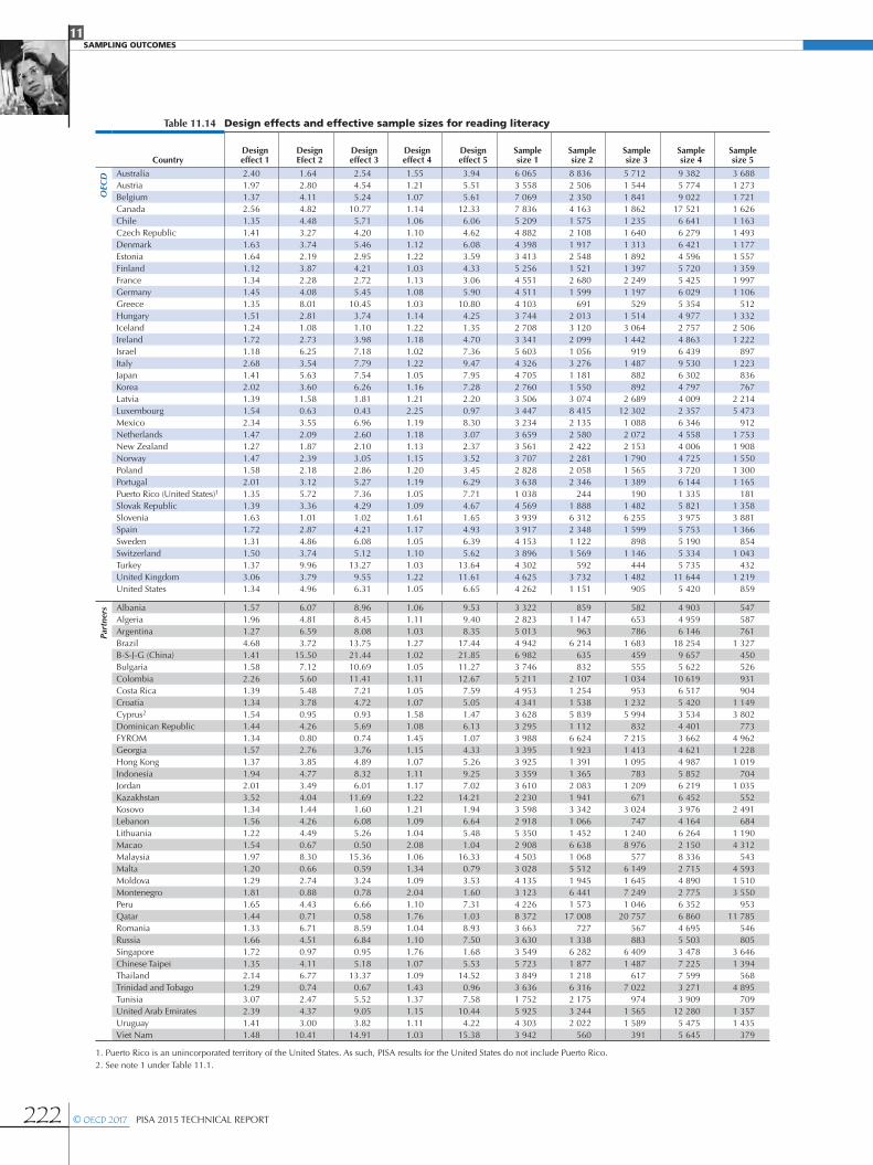
11SAMPLING OUTCOMES
222 © OECD 2017 PISA 2015 TECHNICAL REPORT
Table 11.14 Design effects and effective sample sizes for reading literacy
CountryDesign effect 1
Design Efect 2
Design effect 3
Design effect 4
Design effect 5
Sample size 1
Sample size 2
Sample size 3
Sample size 4
Sample size 5
OEC
D Australia 2.40 1.64 2.54 1.55 3.94 6 065 8 836 5 712 9 382 3 688Austria 1.97 2.80 4.54 1.21 5.51 3 558 2 506 1 544 5 774 1 273Belgium 1.37 4.11 5.24 1.07 5.61 7 069 2 350 1 841 9 022 1 721Canada 2.56 4.82 10.77 1.14 12.33 7 836 4 163 1 862 17 521 1 626Chile 1.35 4.48 5.71 1.06 6.06 5 209 1 575 1 235 6 641 1 163Czech Republic 1.41 3.27 4.20 1.10 4.62 4 882 2 108 1 640 6 279 1 493Denmark 1.63 3.74 5.46 1.12 6.08 4 398 1 917 1 313 6 421 1 177Estonia 1.64 2.19 2.95 1.22 3.59 3 413 2 548 1 892 4 596 1 557Finland 1.12 3.87 4.21 1.03 4.33 5 256 1 521 1 397 5 720 1 359France 1.34 2.28 2.72 1.13 3.06 4 551 2 680 2 249 5 425 1 997Germany 1.45 4.08 5.45 1.08 5.90 4 511 1 599 1 197 6 029 1 106Greece 1.35 8.01 10.45 1.03 10.80 4 103 691 529 5 354 512Hungary 1.51 2.81 3.74 1.14 4.25 3 744 2 013 1 514 4 977 1 332Iceland 1.24 1.08 1.10 1.22 1.35 2 708 3 120 3 064 2 757 2 506Ireland 1.72 2.73 3.98 1.18 4.70 3 341 2 099 1 442 4 863 1 222Israel 1.18 6.25 7.18 1.02 7.36 5 603 1 056 919 6 439 897Italy 2.68 3.54 7.79 1.22 9.47 4 326 3 276 1 487 9 530 1 223Japan 1.41 5.63 7.54 1.05 7.95 4 705 1 181 882 6 302 836Korea 2.02 3.60 6.26 1.16 7.28 2 760 1 550 892 4 797 767Latvia 1.39 1.58 1.81 1.21 2.20 3 506 3 074 2 689 4 009 2 214Luxembourg 1.54 0.63 0.43 2.25 0.97 3 447 8 415 12 302 2 357 5 473Mexico 2.34 3.55 6.96 1.19 8.30 3 234 2 135 1 088 6 346 912Netherlands 1.47 2.09 2.60 1.18 3.07 3 659 2 580 2 072 4 558 1 753New Zealand 1.27 1.87 2.10 1.13 2.37 3 561 2 422 2 153 4 006 1 908Norway 1.47 2.39 3.05 1.15 3.52 3 707 2 281 1 790 4 725 1 550Poland 1.58 2.18 2.86 1.20 3.45 2 828 2 058 1 565 3 720 1 300Portugal 2.01 3.12 5.27 1.19 6.29 3 638 2 346 1 389 6 144 1 165Puerto Rico (United States)1 1.35 5.72 7.36 1.05 7.71 1 038 244 190 1 335 181Slovak Republic 1.39 3.36 4.29 1.09 4.67 4 569 1 888 1 482 5 821 1 358Slovenia 1.63 1.01 1.02 1.61 1.65 3 939 6 312 6 255 3 975 3 881Spain 1.72 2.87 4.21 1.17 4.93 3 917 2 348 1 599 5 753 1 366Sweden 1.31 4.86 6.08 1.05 6.39 4 153 1 122 898 5 190 854Switzerland 1.50 3.74 5.12 1.10 5.62 3 896 1 569 1 146 5 334 1 043Turkey 1.37 9.96 13.27 1.03 13.64 4 302 592 444 5 735 432United Kingdom 3.06 3.79 9.55 1.22 11.61 4 625 3 732 1 482 11 644 1 219United States 1.34 4.96 6.31 1.05 6.65 4 262 1 151 905 5 420 859
Part
ners Albania 1.57 6.07 8.96 1.06 9.53 3 322 859 582 4 903 547
Algeria 1.96 4.81 8.45 1.11 9.40 2 823 1 147 653 4 959 587Argentina 1.27 6.59 8.08 1.03 8.35 5 013 963 786 6 146 761Brazil 4.68 3.72 13.75 1.27 17.44 4 942 6 214 1 683 18 254 1 327B-S-J-G (China) 1.41 15.50 21.44 1.02 21.85 6 982 635 459 9 657 450Bulgaria 1.58 7.12 10.69 1.05 11.27 3 746 832 555 5 622 526Colombia 2.26 5.60 11.41 1.11 12.67 5 211 2 107 1 034 10 619 931Costa Rica 1.39 5.48 7.21 1.05 7.59 4 953 1 254 953 6 517 904Croatia 1.34 3.78 4.72 1.07 5.05 4 341 1 538 1 232 5 420 1 149Cyprus2 1.54 0.95 0.93 1.58 1.47 3 628 5 839 5 994 3 534 3 802Dominican Republic 1.44 4.26 5.69 1.08 6.13 3 295 1 112 832 4 401 773FYROM 1.34 0.80 0.74 1.45 1.07 3 988 6 624 7 215 3 662 4 962Georgia 1.57 2.76 3.76 1.15 4.33 3 395 1 923 1 413 4 621 1 228Hong Kong 1.37 3.85 4.89 1.07 5.26 3 925 1 391 1 095 4 987 1 019Indonesia 1.94 4.77 8.32 1.11 9.25 3 359 1 365 783 5 852 704Jordan 2.01 3.49 6.01 1.17 7.02 3 610 2 083 1 209 6 219 1 035Kazakhstan 3.52 4.04 11.69 1.22 14.21 2 230 1 941 671 6 452 552Kosovo 1.34 1.44 1.60 1.21 1.94 3 598 3 342 3 024 3 976 2 491Lebanon 1.56 4.26 6.08 1.09 6.64 2 918 1 066 747 4 164 684Lithuania 1.22 4.49 5.26 1.04 5.48 5 350 1 452 1 240 6 264 1 190Macao 1.54 0.67 0.50 2.08 1.04 2 908 6 638 8 976 2 150 4 312Malaysia 1.97 8.30 15.36 1.06 16.33 4 503 1 068 577 8 336 543Malta 1.20 0.66 0.59 1.34 0.79 3 028 5 512 6 149 2 715 4 593Moldova 1.29 2.74 3.24 1.09 3.53 4 135 1 945 1 645 4 890 1 510Montenegro 1.81 0.88 0.78 2.04 1.60 3 123 6 441 7 249 2 775 3 550Peru 1.65 4.43 6.66 1.10 7.31 4 226 1 573 1 046 6 352 953Qatar 1.44 0.71 0.58 1.76 1.03 8 372 17 008 20 757 6 860 11 785Romania 1.33 6.71 8.59 1.04 8.93 3 663 727 567 4 695 546Russia 1.66 4.51 6.84 1.10 7.50 3 630 1 338 883 5 503 805Singapore 1.72 0.97 0.95 1.76 1.68 3 549 6 282 6 409 3 478 3 646Chinese Taipei 1.35 4.11 5.18 1.07 5.53 5 723 1 877 1 487 7 225 1 394Thailand 2.14 6.77 13.37 1.09 14.52 3 849 1 218 617 7 599 568Trinidad and Tobago 1.29 0.74 0.67 1.43 0.96 3 636 6 316 7 022 3 271 4 895Tunisia 3.07 2.47 5.52 1.37 7.58 1 752 2 175 974 3 909 709United Arab Emirates 2.39 4.37 9.05 1.15 10.44 5 925 3 244 1 565 12 280 1 357Uruguay 1.41 3.00 3.82 1.11 4.22 4 303 2 022 1 589 5 475 1 435Viet Nam 1.48 10.41 14.91 1.03 15.38 3 942 560 391 5 645 379
1. Puerto Rico is an unincorporated territory of the United States. As such, PISA results for the United States do not include Puerto Rico. 2. See note 1 under Table 11.1.
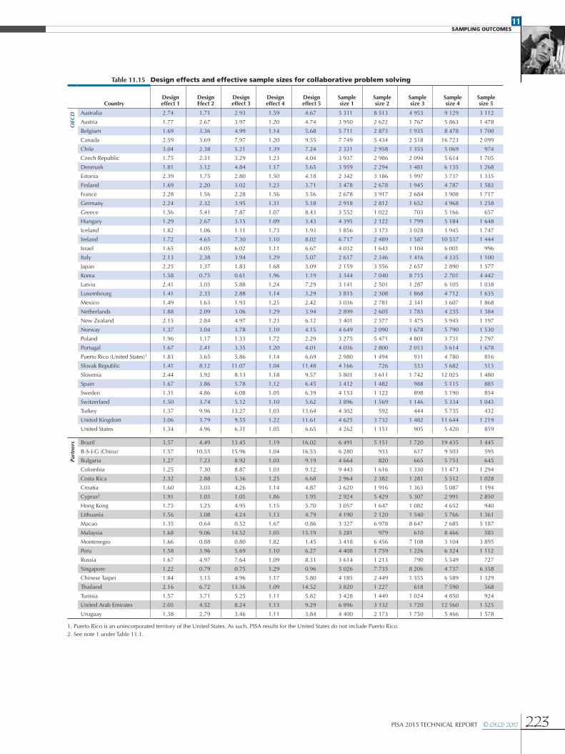
11SAMPLING OUTCOMES
PISA 2015 TECHNICAL REPORT © OECD 2017 223
Table 11.15 Design effects and effective sample sizes for collaborative problem solving
CountryDesign effect 1
Design Efect 2
Design effect 3
Design effect 4
Design effect 5
Sample size 1
Sample size 2
Sample size 3
Sample size 4
Sample size 5
OEC
D Australia 2.74 1.71 2.93 1.59 4.67 5 311 8 513 4 953 9 129 3 112
Austria 1.77 2.67 3.97 1.20 4.74 3 950 2 622 1 767 5 863 1 478
Belgium 1.69 3.36 4.99 1.14 5.68 5 711 2 873 1 935 8 478 1 700
Canada 2.59 3.69 7.97 1.20 9.55 7 749 5 434 2 518 16 723 2 099
Chile 3.04 2.38 5.21 1.39 7.24 2 321 2 958 1 355 5 069 974
Czech Republic 1.75 2.31 3.29 1.23 4.04 3 937 2 986 2 094 5 614 1 705
Denmark 1.81 3.12 4.84 1.17 5.65 3 959 2 294 1 481 6 135 1 268
Estonia 2.39 1.75 2.80 1.50 4.18 2 342 3 186 1 997 3 737 1 335
Finland 1.69 2.20 3.02 1.23 3.71 3 478 2 678 1 945 4 787 1 583
France 2.28 1.56 2.28 1.56 3.56 2 678 3 917 2 684 3 908 1 717
Germany 2.24 2.32 3.95 1.31 5.18 2 918 2 812 1 652 4 968 1 258
Greece 1.56 5.41 7.87 1.07 8.43 3 552 1 022 703 5 166 657
Hungary 1.29 2.67 3.15 1.09 3.43 4 395 2 122 1 799 5 184 1 648
Iceland 1.82 1.06 1.11 1.73 1.93 1 856 3 173 3 028 1 945 1 747
Ireland 1.72 4.65 7.30 1.10 8.02 6 717 2 489 1 587 10 537 1 444
Israel 1.65 4.05 6.02 1.11 6.67 4 032 1 643 1 104 6 001 996
Italy 2.13 2.38 3.94 1.29 5.07 2 617 2 346 1 416 4 335 1 100
Japan 2.25 1.37 1.83 1.68 3.09 2 159 3 556 2 657 2 890 1 577
Korea 1.58 0.75 0.61 1.96 1.19 3 344 7 040 8 715 2 701 4 442
Latvia 2.41 3.03 5.88 1.24 7.29 3 141 2 501 1 287 6 105 1 038
Luxembourg 1.41 2.33 2.88 1.14 3.29 3 815 2 308 1 868 4 712 1 635
Mexico 1.49 1.63 1.93 1.25 2.42 3 036 2 781 2 341 3 607 1 868
Netherlands 1.88 2.09 3.06 1.29 3.94 2 899 2 605 1 783 4 235 1 384
New Zealand 2.15 2.84 4.97 1.23 6.12 3 401 2 577 1 475 5 945 1 197
Norway 1.37 3.04 3.78 1.10 4.15 4 649 2 090 1 678 5 790 1 530
Poland 1.96 1.17 1.33 1.72 2.29 3 275 5 471 4 801 3 731 2 797
Portugal 1.67 2.41 3.35 1.20 4.01 4 036 2 800 2 013 5 614 1 678
Puerto Rico (United States)1 1.83 3.65 5.86 1.14 6.69 2 980 1 494 931 4 780 816
Slovak Republic 1.41 8.12 11.07 1.04 11.48 4 166 726 533 5 682 513
Slovenia 2.44 3.92 8.13 1.18 9.57 5 801 3 611 1 742 12 025 1 480
Spain 1.67 3.86 5.78 1.12 6.45 3 412 1 482 988 5 115 885
Sweden 1.31 4.86 6.08 1.05 6.39 4 153 1 122 898 5 190 854
Switzerland 1.50 3.74 5.12 1.10 5.62 3 896 1 569 1 146 5 334 1 043
Turkey 1.37 9.96 13.27 1.03 13.64 4 302 592 444 5 735 432
United Kingdom 3.06 3.79 9.55 1.22 11.61 4 625 3 732 1 482 11 644 1 219
United States 1.34 4.96 6.31 1.05 6.65 4 262 1 151 905 5 420 859
Part
ners Brazil 3.57 4.49 13.45 1.19 16.02 6 491 5 151 1 720 19 435 1 445
B-S-J-G (China) 1.57 10.55 15.96 1.04 16.53 6 280 933 617 9 503 595
Bulgaria 1.27 7.23 8.92 1.03 9.19 4 664 820 665 5 753 645
Colombia 1.25 7.30 8.87 1.03 9.12 9 443 1 616 1 330 11 473 1 294
Costa Rica 2.32 2.88 5.36 1.25 6.68 2 964 2 382 1 281 5 512 1 028
Croatia 1.60 3.03 4.26 1.14 4.87 3 620 1 916 1 363 5 087 1 194
Cyprus2 1.91 1.03 1.05 1.86 1.95 2 924 5 429 5 307 2 991 2 850
Hong Kong 1.75 3.25 4.95 1.15 5.70 3 057 1 647 1 082 4 652 940
Lithuania 1.56 3.08 4.24 1.13 4.79 4 190 2 120 1 540 5 766 1 361
Macao 1.35 0.64 0.52 1.67 0.86 3 327 6 978 8 647 2 685 5 187
Malaysia 1.68 9.06 14.52 1.05 15.19 5 281 979 610 8 466 583
Montenegro 1.66 0.88 0.80 1.82 1.45 3 418 6 456 7 108 3 104 3 895
Peru 1.58 3.96 5.69 1.10 6.27 4 408 1 759 1 226 6 324 1 112
Russia 1.67 4.97 7.64 1.09 8.31 3 614 1 213 790 5 549 727
Singapore 1.22 0.79 0.75 1.29 0.96 5 026 7 735 8 206 4 737 6 358
Chinese Taipei 1.84 3.15 4.96 1.17 5.80 4 185 2 449 1 555 6 589 1 329
Thailand 2.16 6.72 13.36 1.09 14.52 3 820 1 227 618 7 590 568
Tunisia 1.57 3.71 5.25 1.11 5.82 3 428 1 449 1 024 4 850 924
United Arab Emirates 2.05 4.52 8.24 1.13 9.29 6 896 3 132 1 720 12 560 1 525
Uruguay 1.38 2.79 3.46 1.11 3.84 4 400 2 173 1 750 5 466 1 578
1. Puerto Rico is an unincorporated territory of the United States. As such, PISA results for the United States do not include Puerto Rico. 2. See note 1 under Table 11.1.
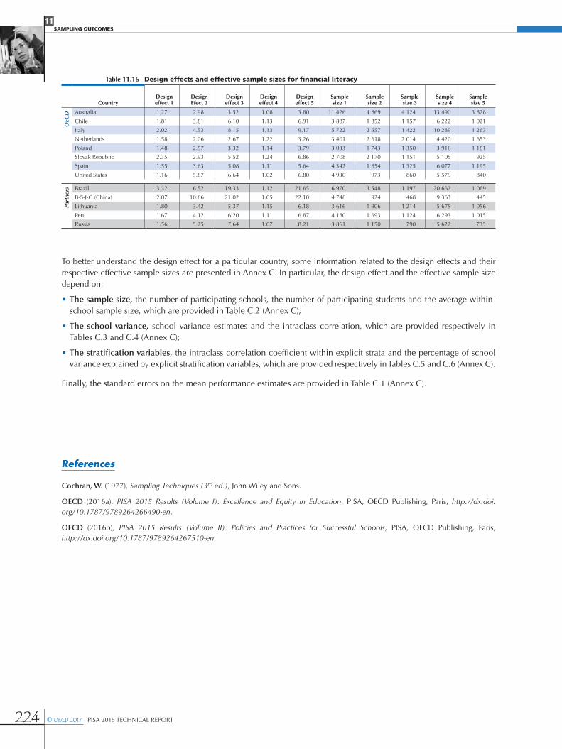
11SAMPLING OUTCOMES
224 © OECD 2017 PISA 2015 TECHNICAL REPORT
To better understand the design effect for a particular country, some information related to the design effects and their respective effective sample sizes are presented in Annex C. In particular, the design effect and the effective sample size depend on:
• The sample size, the number of participating schools, the number of participating students and the average within-school sample size, which are provided in Table C.2 (Annex C);
• The school variance, school variance estimates and the intraclass correlation, which are provided respectively in Tables C.3 and C.4 (Annex C);
• The stratification variables, the intraclass correlation coefficient within explicit strata and the percentage of school variance explained by explicit stratification variables, which are provided respectively in Tables C.5 and C.6 (Annex C).
Finally, the standard errors on the mean performance estimates are provided in Table C.1 (Annex C).
References
Cochran, W. (1977), Sampling Techniques (3rd ed.), John Wiley and Sons.
OECD (2016a), PISA 2015 Results (Volume I): Excellence and Equity in Education, PISA, OECD Publishing, Paris, http://dx.doi.org/10.1787/9789264266490-en.
OECD (2016b), PISA 2015 Results (Volume II): Policies and Practices for Successful Schools, PISA, OECD Publishing, Paris, http://dx.doi.org/10.1787/9789264267510-en.
Table 11.16 Design effects and effective sample sizes for financial literacy
CountryDesign effect 1
Design Efect 2
Design effect 3
Design effect 4
Design effect 5
Sample size 1
Sample size 2
Sample size 3
Sample size 4
Sample size 5
OEC
D Australia 1.27 2.98 3.52 1.08 3.80 11 426 4 869 4 124 13 490 3 828
Chile 1.81 3.81 6.10 1.13 6.91 3 887 1 852 1 157 6 222 1 021
Italy 2.02 4.53 8.15 1.13 9.17 5 722 2 557 1 422 10 289 1 263
Netherlands 1.58 2.06 2.67 1.22 3.26 3 401 2 618 2 014 4 420 1 653
Poland 1.48 2.57 3.32 1.14 3.79 3 033 1 743 1 350 3 916 1 181
Slovak Republic 2.35 2.93 5.52 1.24 6.86 2 708 2 170 1 151 5 105 925
Spain 1.55 3.63 5.08 1.11 5.64 4 342 1 854 1 325 6 077 1 195
United States 1.16 5.87 6.64 1.02 6.80 4 930 973 860 5 579 840
Part
ners Brazil 3.32 6.52 19.33 1.12 21.65 6 970 3 548 1 197 20 662 1 069
B-S-J-G (China) 2.07 10.66 21.02 1.05 22.10 4 746 924 468 9 363 445
Lithuania 1.80 3.42 5.37 1.15 6.18 3 616 1 906 1 214 5 675 1 056
Peru 1.67 4.12 6.20 1.11 6.87 4 180 1 693 1 124 6 293 1 015
Russia 1.56 5.25 7.64 1.07 8.21 3 861 1 150 790 5 622 735
Related Documents