#11 QUEUEING THEORY Systems 303 - Fall 2000 Instructor: Peter M. Hahn [email protected].

#11QUEUEING THEORY

Systems 303 - Fall 2000

Instructor: Peter M. Hahn

[email protected]

QUEUEING THEORY

• For simple service/manufacturing situations one can analyze steady-state system performance

• An important facilitator is the governing Poisson process model for arrivals and for service times

• We present a difference-equation analytical approach• And therewith generate the probability distribution of

system occupancy for the M/M/1 server queue• The resulting steady-state M/M/1 occupancy

probabilities are entirely independent of time• This probability distribution permits us to calculate

desired service performance measures

THE DISTRIBUTION OF ARRIVALS• Given N arrivals randomly distributed in [0,T]. The

RV X is the number of arrivals in a small interval 0 T

• The N arrivals are IID uniformly over [0,T]• X is therefore governed by a binomial distribution

with p=/T, q=(T- )/T and N=number of arrivals

e.g., P(3 arrivals) = f3 =N3 ⎛ ⎝ ⎜

⎞ ⎠ ⎟T ⎛ ⎝ ⎜ ⎞

⎠ ⎟3 T −

T ⎛ ⎝ ⎜ ⎞

⎠ ⎟N−3

P( 1 )at least arrival=1− f0 =1−T −T

⎛ ⎝ ⎜ ⎞

⎠ ⎟N

whereN T=m= . expected no of arrivals in

THE DISTRIBUTION OF ARRIVALS

• Keeping m constant and letting T∞ and N ∞, the binomial distribution becomes a Poisson distribution with m= N/T= , i.e.,

• It turns out that the probability of an arrival in a given interval is independent of what happens before or after . Can you explain why?

• The distribution of arrivals has the same shape no matter what the size of (remember T∞)

P(X =n) = fn =e−mmn

n!=e− ( )

n

n!

P(X =1) = f1 =e−mm=e− ( )

THE DISTRIBUTION OF ARRIVALS

• Let Y = the time from a specified time t0 until the first arrival occurs

• But, the event Y > y is equivalent to the event ‘no call has arrived in time interval [t0, t0+y]. Thus,

• This is the exponential distribution about which we talked so much

FY (y) =P Y ≤y( ) =1−P Y > y( )

FY (y) =1− f0 =1−e−mm0

0!=1−e−m=1−e−y

which corresponds to

fY (y) =e−y ( )by differentiation

THE CONCEPT OF A SERVER

• A server starts a service operation upon an arrival• It cannot start another service operation until the

previous operation is finished• Arrivals during an operation must wait in queue (or

buffer) until all operations are completed• Time for the operation is usually a random variable• Two rules govern the server

– The average rate at which operations can be completed must be higher than or equal to the average arrival rate

– Instantaneous arrival rate may be higher than

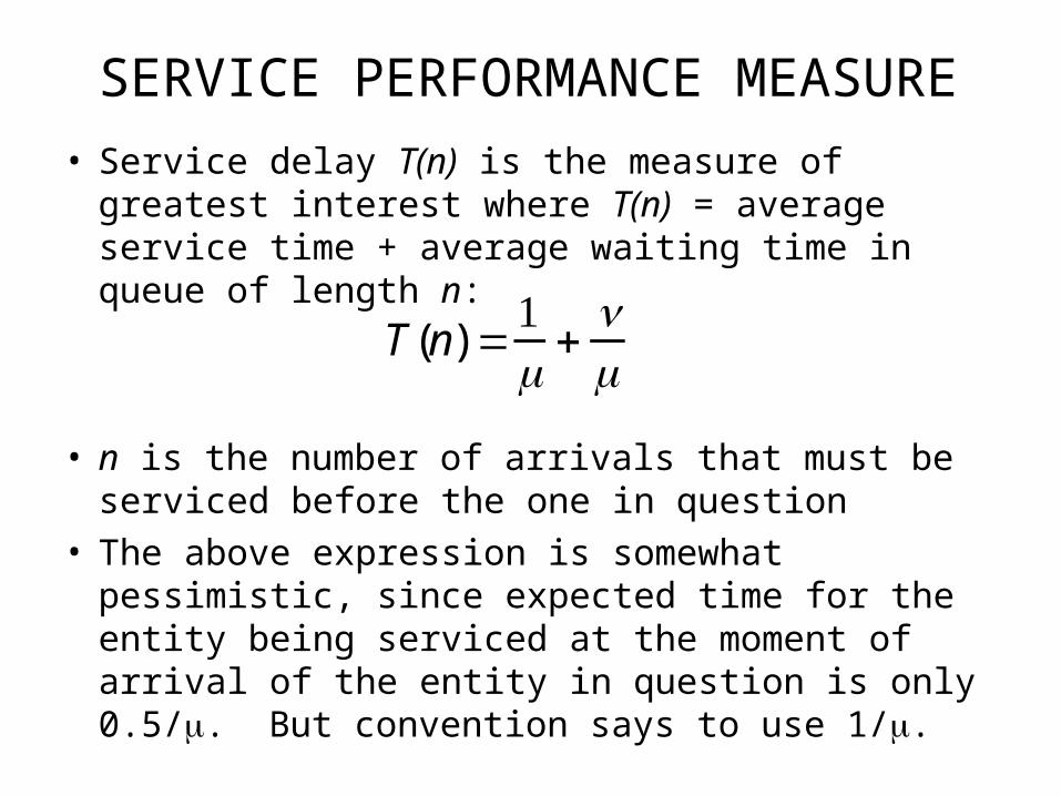
SERVICE PERFORMANCE MEASURE

• Service delay T(n) is the measure of greatest interest where T(n) = average service time + average waiting time in queue of length n:

• n is the number of arrivals that must be serviced before the one in question

• The above expression is somewhat pessimistic, since expected time for the entity being serviced at the moment of arrival of the entity in question is only 0.5/. But convention says to use 1/.

T(n) =1+n

THE CONCEPT OF A SERVER

• Queues are characterized by A/B/C where– A is the arrival distribution

– B is the service distribution

– C is the number of independent servers servicing the queue

• An additional element is the service discipline (e.g., FIFO, FILO, priority, etc.) since n depends on this

• Maximum queue length and queue interdependence are also factors but are seldom considered in theory

• A=M stands for Poisson process arrivals• B=M stands for Poisson process service completions

(i.e., exponentially distributed service times)

ANALYSIS OF M/M/1 SYSTEMS

• The Poisson assumptions are good for a great variety of transactions in business and manufacturing

• For this analysis, queue length is not restricted• Consider a small time interval ∆t during which

arrivals and service completions may take place• Later ∆t 0.• The following table holds for M/M/1 systems:

Arrival time statistics Service time statisticsRate = Rat e= f0 = exp(-Δt ) f0 =exp(-Δt )P(1 or mor )e = 1 - exp(-Δt ) P(1 or mor )e = 1 - exp(-Δt )

M/M/1 SERVER SYSTEMS

If now we let Δt→ 0 f0 → 1−ΔtυP(1 or more) → Δtυ f1 → ΔtυP(2 )or more=P(1 or more)− f1 → 0

Letting υ be either or ( )arrival or departure

f0 =e−Δtυ =1−Δtυ + Δtυ( )2

2!− Δtυ( )3

3!+ −⋅⋅⋅

P(1 or more) =1−e−Δtυ =Δtυ − Δtυ( )2

2!+ Δtυ( )3

3!−+⋅⋅⋅

and f1 =e−ΔtυΔtυ =Δtυ − Δtυ( )2 +

Δtυ( )3

2!−+⋅⋅⋅

M/M/1 SERVER SYSTEMS

• Therefore, during ∆t the probability of more than 1 arrival or more than 1 departure becomes insignificantly small

• Thus, if the queue holds n at the end of ∆t, then at the start of ∆t there could have been no more than n+1 nor fewer than n-1 in the queue

• The probability of n in queue at time t+∆t may then be written in terms of probabilities of queue content at time t

• Recall that ∆t to ∆t events are independent

M/M/1 SERVER SYSTEMSpn (t) =P(n entities in the system at timet)

pn(t+ Δt) =pn(t) ⋅P(0 0 arrivals and service completionsor

1 1 )exactly arrival and service completion

+pn+1(t)⋅P(0 1 )arrivals and service completion

+pn−1(t)⋅P(1 0 )arrival and service completions

=pn(t) ⋅ 1−Δt( ) 1−Δt( ) + Δt⋅Δt[ ]

+pn+1(t)⋅Δt 1−Δt( )[ ] + pn−1(t)⋅Δt 1−Δt( )[ ]

LettingΔt→ 0

pn(t+ Δt) =pn(t) ⋅1−Δt−Δt( ) + pn+1(t)⋅Δt+ pn−1 (t) ⋅Δt

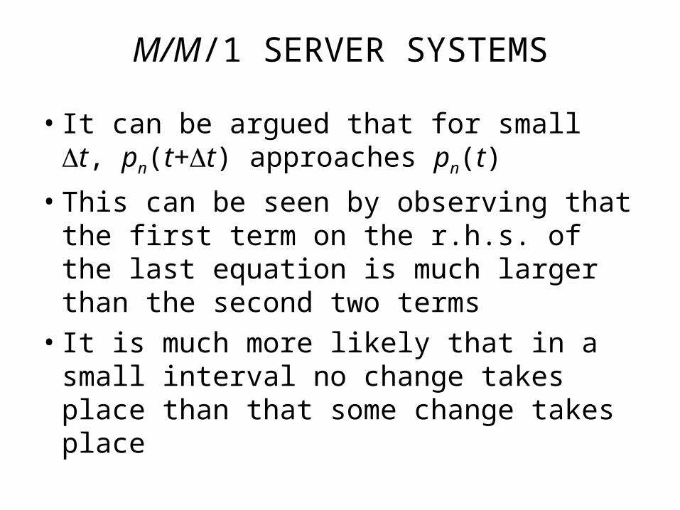
M/M/1 SERVER SYSTEMS

• It can be argued that for small Δt, pn(t+Δt) approaches pn(t)

• This can be seen by observing that the first term on the r.h.s. of the last equation is much larger than the second two terms

• It is much more likely that in a small interval no change takes place than that some change takes place

M/M/1 SERVER SYSTEMS

• Thus, letting pn(t+Δt) —› pn(t)

• This final equation governs the process of arrivals and service completions affecting n

pn (t + Δt) =pn(t) =pn(t) ⋅1−Δt−Δt( )

+pn+1 (t) ⋅Δt + pn−1(t)⋅Δtor

pn(t) ⋅Δt+ Δt( ) =pn+1 (t) ⋅Δt + pn−1(t)⋅Δt

pn(t)⋅ +ν( ) =pn+1 (t) ⋅ + pn−1 (t) ⋅

M/M/1 INITIAL CONDITIONS– No system reduction poss. with an empty system– System occupancy probability must sum to unity

p0 (t + Δt) =p0 (t)P(0 . 0 . 1 . 1 .)arr and depart or arr and depart

+ p1 (t)P(0 . 1 .)arr and depart

=p0 (t) 1−Δt( )⋅1+Δt⋅0[ ] + p1(t) Δt 1−Δt( )[ ]

=p0 (t) 1−Δt( ) + p1(t) Δt 1−Δt( )[ ]

ForΔt ,small

p0 (t) =p0 (t) 1−Δt( ) + p1(t)Δt orp0 (t)Δt=p1(t)Δt

p1 (t) =ρp0 (t) whereρ =ν

SOLVING M/M/1 SYS. RECURSIVELY

( + )p1(t) =p2 (t) + p0 (t) ( 14)from slide

or(ρ +1)ρp0 (t) =p2 (t) + ρp0 (t)

p2 (t) =ρ2p0 (t)

Similarly:

( + )p2 (t) =p3 (t) + p1 (t) ( 14)from slide

(ρ +1)ρ2p0 (t) =p3 (t) + ρp1(t) =p3 (t) + ρ2p0 (t)

p3(t) =ρ3p0 (t)

In general:

pn(t) =ρnp0 (t)

M/M/1 SYSTEM SECOND CONDITION

pn (t)

n=0

∞

∑ =1

But noting that:

pn(t)

n=0

∞

∑ =p0 (t) ρn

n=0

∞

∑ =p0 (t)1−ρ

becauseρ =<1

So that:p0 (t)1−ρ

=1 orp0 (t) =1−ρ

and

pn(t) = 1−ρ( )ρn =pn

RESULTS OF M/M/1 ANALYSIS

• We have thus produced a complete distribution of system occupancy for the M/M/1 server system

• We have also proven that M/M/1 occupancy probabilities are entirely independent of time

• This assures us that the random process that governs M/M/1 system occupancy is strictly stationary

• Similar analyses can be performed for other, more complex queuing models

• From the above discrete probability distribution, we can now calculate certain desired service performance measures

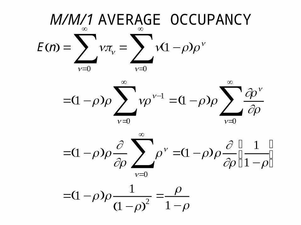
M/M/1 AVERAGE OCCUPANCY

E n( ) = npnn=0

∞

∑ = n(1−ρ)ρn

n=0

∞

∑=(1−ρ)ρ nρn−1

n=0

∞

∑ =(1−ρ)ρ ∂ρn

∂ρn=0

∞

∑=(1−ρ)ρ ∂

∂ρρn

n=0

∞

∑ =(1−ρ)ρ ∂∂ρ

11−ρ ⎛

⎝ ⎜

⎞

⎠ ⎟

=(1−ρ)ρ 11−ρ( )2

= ρ1−ρ

M/M/1 AVERAGE SERVICE DELAY

• From slide 7

E T n( )[ ] =E1+ n

⎡

⎣ ⎢ ⎤

⎦ ⎥=1+ ρ1−ρ

1

=1

11−ρ ⎛

⎝ ⎜

⎞

⎠ ⎟=

1

− ⎛ ⎝ ⎜

⎞ ⎠ ⎟

=1

−

M/M/1 SYSTEM OVERFLOW (n > N)

P(n > N) = pnn=N+1

∞

∑ =(1−ρ) ρn

n=N+1

∞

∑ Lettingm=n−N −1 orn=m+ N +1

P(n> N) =(1−ρ) ρm+N+1

m=0

∞

∑=(1−ρ)ρN+1 ρm

m=0

∞

∑ =(1−ρ)ρ N+1 11−ρ ⎛

⎝ ⎜

⎞

⎠ ⎟

=ρ N+1

HOMEWORK #11Read Sections 6.1-6.4 in B,C,N&N

Inter-arrival and service times at a copier are exponentially distributed. The average copying job takes 3 minutes. There are on the average 12 copying jobs arriving per hour. No job quits the queue.

a) Calculate the probabilities for 1, 2, 3, and (4 or more) jobs at the copier

b) What is the percent time that the copier is occupied?

c) With a different person occupied with each job, how many people are tied up on the average in copying?

d) What is the average time for a copying job?

e) What is the average waiting time for the copier?