ECE 333 © 2002 – 2017 George Gross, University of Illinois at Urbana-Champaign, All Rights Reserved. 1 ECE 333 – GREEN ELECTRIC ENERGY 11. Basic Concepts in Power System Economics George Gross Department of Electrical and Computer Engineering University of Illinois at Urbana–Champaign

Welcome message from author
This document is posted to help you gain knowledge. Please leave a comment to let me know what you think about it! Share it to your friends and learn new things together.
Transcript
ECE 333 © 2002 – 2017 George Gross, University of Illinois at Urbana-Champaign, All Rights Reserved. 1
ECE 333 – GREEN ELECTRIC ENERGY
11. Basic Concepts in Power System Economics
George Gross
Department of Electrical and Computer EngineeringUniversity of Illinois at Urbana–Champaign
ECE 333 © 2002 – 2017 George Gross, University of Illinois at Urbana-Champaign, All Rights Reserved. 2
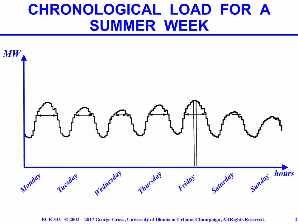
CHRONOLOGICAL LOAD FOR A SUMMER WEEK
MW
hours
ECE 333 © 2002 – 2017 George Gross, University of Illinois at Urbana-Champaign, All Rights Reserved. 3
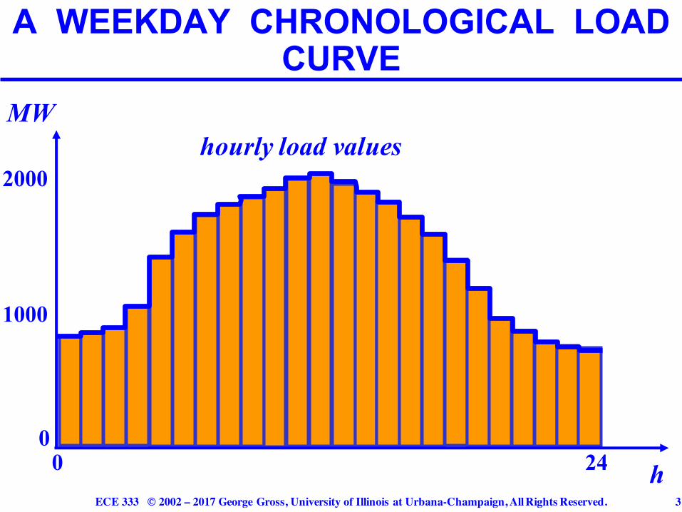
A WEEKDAY CHRONOLOGICAL LOAD CURVE
hourly load valuesMW
2000
0
1000
0 24 h
ECE 333 © 2002 – 2017 George Gross, University of Illinois at Urbana-Champaign, All Rights Reserved. 4
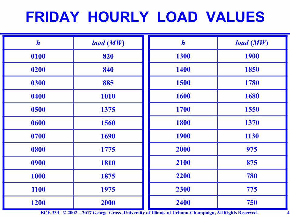
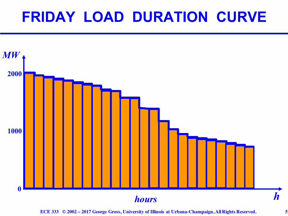
FRIDAY HOURLY LOAD VALUESh load (MW)
0100 820
0200 840
0300 885
0400 1010
0500 1375
0600 1560
0700 1690
0800 1775
0900 1810
1000 1875
1100 1975
1200 2000
h load (MW)
1300 1900
1400 1850
1500 1780
1600 1680
1700 1550
1800 1370
1900 1130
2000 975
2100 875
2200 780
2300 775
2400 750
ECE 333 © 2002 – 2017 George Gross, University of Illinois at Urbana-Champaign, All Rights Reserved. 5
FRIDAY LOAD DURATION CURVE
hours
MW
2000
0
1000
h
ECE 333 © 2002 – 2017 George Gross, University of Illinois at Urbana-Champaign, All Rights Reserved. 6
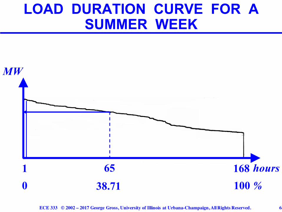
LOAD DURATION CURVE FOR A SUMMER WEEK
MW
138.71
168100 %0
hours65
ECE 333 © 2002 – 2017 George Gross, University of Illinois at Urbana-Champaign, All Rights Reserved. 7
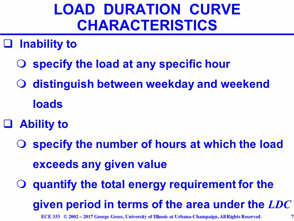
q Inability to m specify the load at any specific hourm distinguish between weekday and weekend
loadsq Ability to
m specify the number of hours at which the load exceeds any given value
m quantify the total energy requirement for the given period in terms of the area under the LDC
LOAD DURATION CURVE CHARACTERISTICS

ECE 333 © 2002 – 2017 George Gross, University of Illinois at Urbana-Champaign, All Rights Reserved. 8
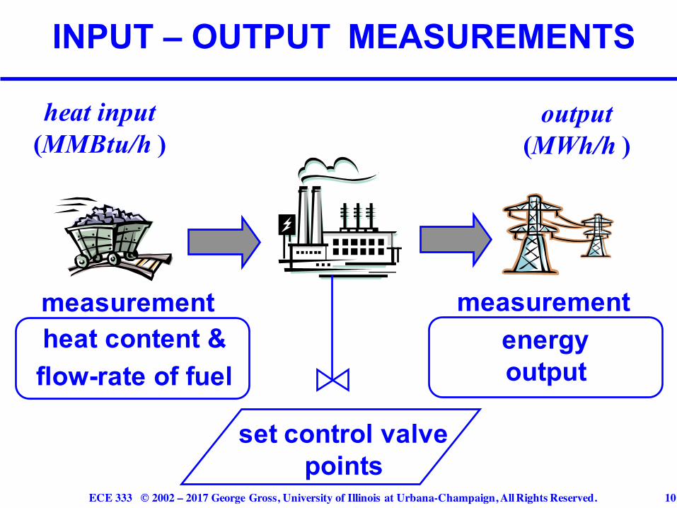
q The costs of generation by a conventional unit
are described by an input-output curve, which
specifies the level of input required to obtain a
required level of output
q Typically, such curves are obtained from actual
measurements and are characterized by their
monotonically non–decreasing shapes
CONVENTIONAL GENERATION UNIT ECONOMICS

ECE 333 © 2002 – 2017 George Gross, University of Illinois at Urbana-Champaign, All Rights Reserved. 9
GENERATION UNIT ECONOMICS
MWh/houtputminc maxc
inputMMBtu/h
orbbl /h
input – output curve
ECE 333 © 2002 – 2017 George Gross, University of Illinois at Urbana-Champaign, All Rights Reserved. 10
INPUT – OUTPUT MEASUREMENTS
heat input(MMBtu/h )
output (MWh/h )
set control valve points
heat content &flow-rate of fuel
energy output
measurement measurement

ECE 333 © 2002 – 2017 George Gross, University of Illinois at Urbana-Champaign, All Rights Reserved. 11
EXAMPLE : CWLP DALLMAN UNITS 1 AND 2
972901835773715659605552499446392336
807570656055504540353025
heat
inpu
t( M
MB
tu/h
)
outp
ut( M
Wh/
h )
ECE 333 © 2002 – 2017 George Gross, University of Illinois at Urbana-Champaign, All Rights Reserved. 12
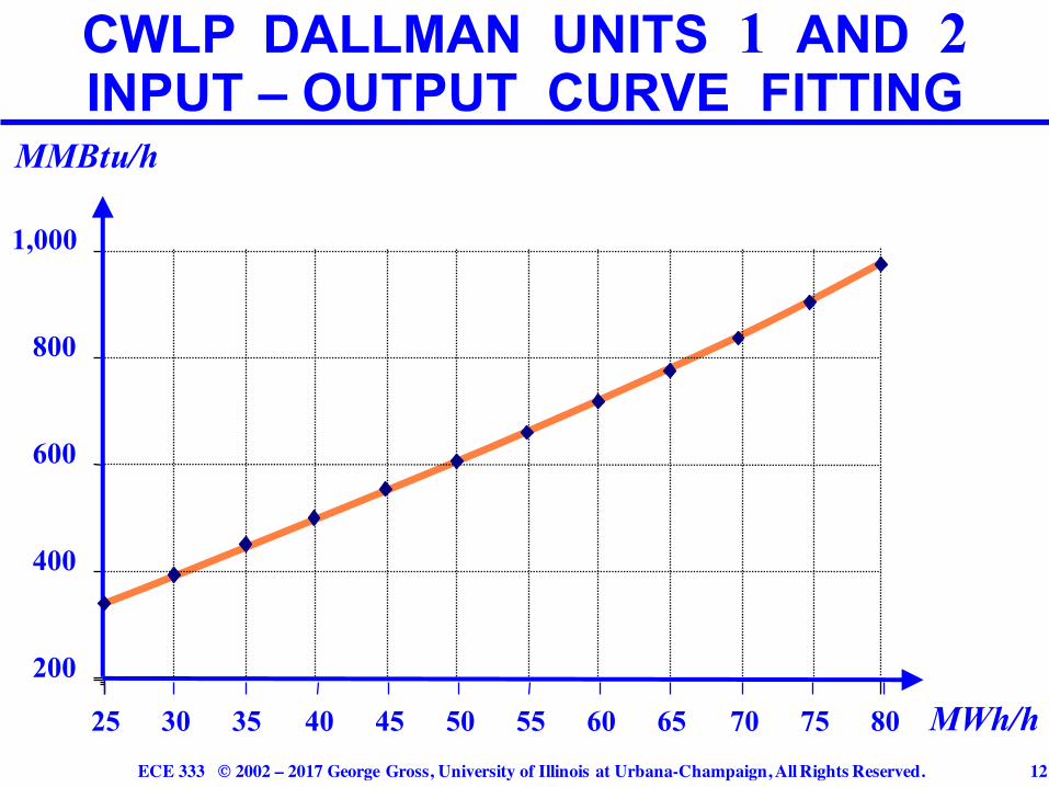
CWLP DALLMAN UNITS 1 AND 2INPUT – OUTPUT CURVE FITTING
MMBtu/h
MWh/h200
400
600
800
1,000
25 30 35 40 45 50 55 60 65 70 75 80
ECE 333 © 2002 – 2017 George Gross, University of Illinois at Urbana-Champaign, All Rights Reserved. 13
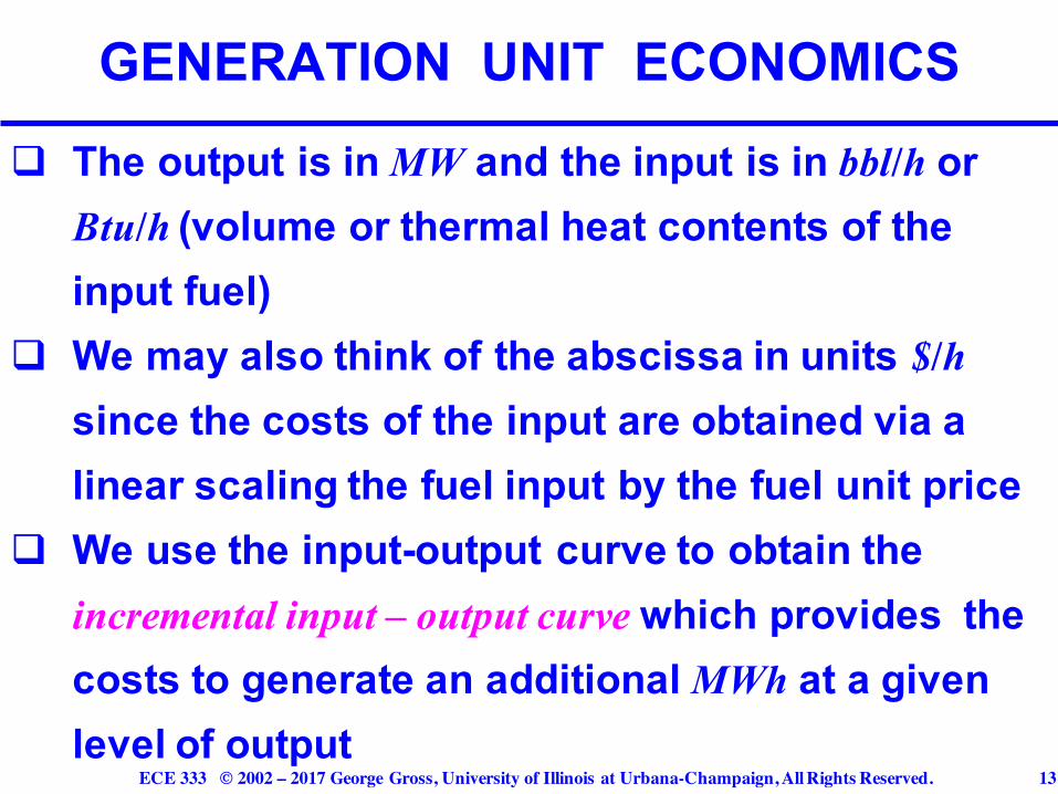
q The output is in MW and the input is in bbl/h or Btu/h (volume or thermal heat contents of the input fuel)
q We may also think of the abscissa in units $/hsince the costs of the input are obtained via a linear scaling the fuel input by the fuel unit price
q We use the input-output curve to obtain the incremental input – output curve which provides the costs to generate an additional MWh at a given level of output
GENERATION UNIT ECONOMICS
ECE 333 © 2002 – 2017 George Gross, University of Illinois at Urbana-Champaign, All Rights Reserved. 14
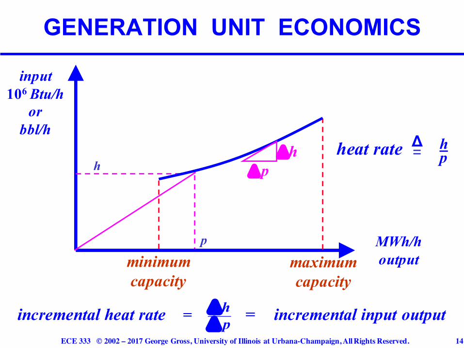
GENERATION UNIT ECONOMICS
incremental heat rate = = incremental input output
heat rate hp=
Δh
p
input 106 Btu/h
orbbl/h
MWh/h outputminimum
capacity
Δh Δ p
maximumcapacity
ΔhΔ p

ECE 333 © 2002 – 2017 George Gross, University of Illinois at Urbana-Champaign, All Rights Reserved. 15
INCREMENTAL CHARACTERISTICS
output in MWh/hminimum
capacitymaximumcapacity
incr
emen
tal h
eat r
ate
106
Btu
/MW
h
ECE 333 © 2002 – 2017 George Gross, University of Illinois at Urbana-Champaign, All Rights Reserved. 16
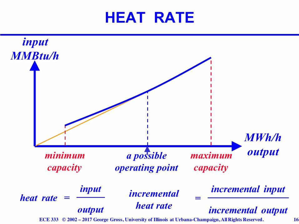
HEAT RATE
a possibleoperating point
MWh/h outputminimum
capacitymaximumcapacity
heat rate =
input
output
incrementalheat rate
=
incremental input
incremental output
input MMBtu/h
ECE 333 © 2002 – 2017 George Gross, University of Illinois at Urbana-Champaign, All Rights Reserved. 17
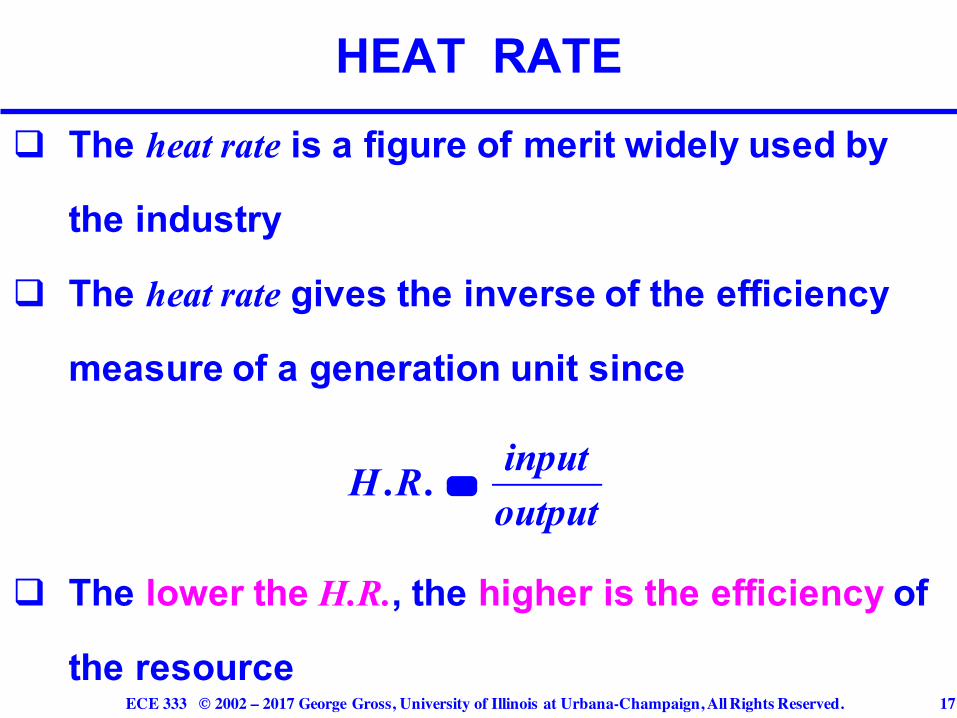
q The heat rate is a figure of merit widely used by
the industry
q The heat rate gives the inverse of the efficiency
measure of a generation unit since
q The lower the H.R., the higher is the efficiency of
the resource
HEAT RATE
H .R. = input
output

ECE 333 © 2002 – 2017 George Gross, University of Illinois at Urbana-Champaign, All Rights Reserved. 18
CWLP DALLMAN UNITS 1 AND 2H. R. & INCREMENTAL H. R. CURVES
heat rate (H.R.) incremental heat rate (I.H.R.)
MMBtu/MWh
9
10
11
12
13
14
25 30 35 40 45 50 55 60 65 70 75 80 MWh/h
ECE 333 © 2002 – 2017 George Gross, University of Illinois at Urbana-Champaign, All Rights Reserved. 19
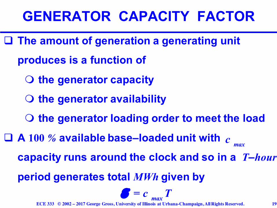
q The amount of generation a generating unit produces is a function of
m the generator capacitym the generator availabilitym the generator loading order to meet the load
q A 100 % available base–loaded unit with capacity runs around the clock and so in a T–hour
period generates total MWh given by
GENERATOR CAPACITY FACTOR
E = c max T
c max
ECE 333 © 2002 – 2017 George Gross, University of Illinois at Urbana-Champaign, All Rights Reserved. 20
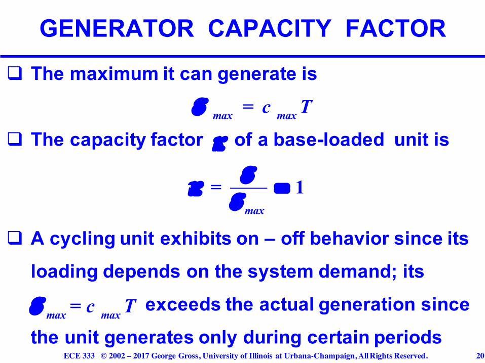
q The maximum it can generate is
q The capacity factor of a base-loaded unit is
q A cycling unit exhibits on – off behavior since its loading depends on the system demand; its
exceeds the actual generation since the unit generates only during certain periods
GENERATOR CAPACITY FACTOR
E max = c max T
κ
κ =
EE max
= 1
E max = c max T
ECE 333 © 2002 – 2017 George Gross, University of Illinois at Urbana-Champaign, All Rights Reserved. 21
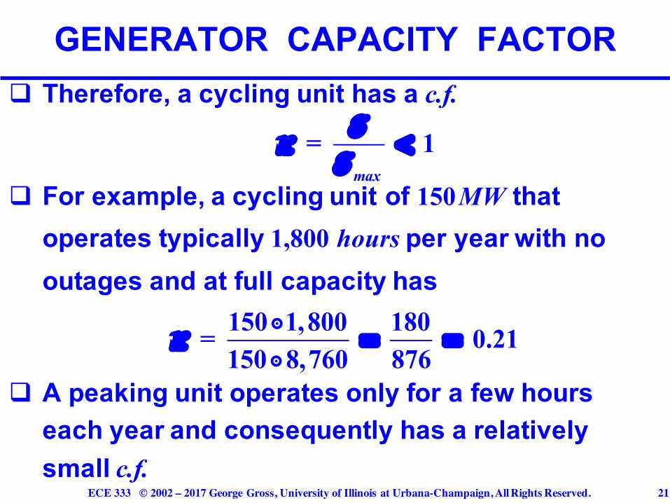
q Therefore, a cycling unit has a c.f.
q For example, a cycling unit of 150MW that operates typically 1,800 hours per year with no outages and at full capacity has
q A peaking unit operates only for a few hours each year and consequently has a relatively small c.f.
GENERATOR CAPACITY FACTOR
κ =
EE max
< 1
κ = 150 ⋅ 1,800
150 ⋅ 8,760= 180
876= 0.21
ECE 333 © 2002 – 2017 George Gross, University of Illinois at Urbana-Champaign, All Rights Reserved. 22
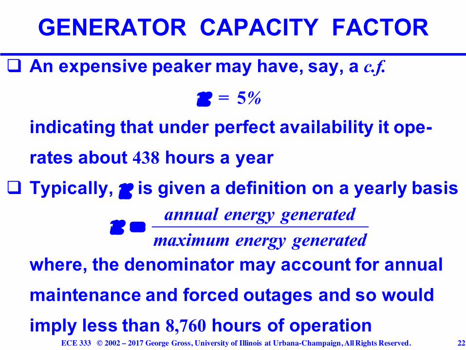
q An expensive peaker may have, say, a c.f.
indicating that under perfect availability it ope-rates about 438 hours a year
q Typically, is given a definition on a yearly basis
where, the denominator may account for annual maintenance and forced outages and so would imply less than 8,760 hours of operation
GENERATOR CAPACITY FACTOR
κ = 5%
κ = annual energy generated
maximum energy generated
κ

ECE 333 © 2002 – 2017 George Gross, University of Illinois at Urbana-Champaign, All Rights Reserved. 23
CAPACITY FACTOR
c. f . =
A 1
A 1 + A 2( )
2A1Ac
MW
time0 % 100 %
load duration curve

ECE 333 © 2002 – 2017 George Gross, University of Illinois at Urbana-Champaign, All Rights Reserved. 24
LOADING OF RESOURCES
unit 1
unit 2
unit 3
unit 4
unit 5unit 6
unit 7
h
MW

ECE 333 © 2002 – 2017 George Gross, University of Illinois at Urbana-Champaign, All Rights Reserved. 25
LOADING OF RESOURCES
Monday Tuesday Wednesday Thursday Friday Saturday Sunday
total available capacity
load
inte
rmed
iate
lo
ad
base load
peak
load
ECE 333 © 2002 – 2017 George Gross, University of Illinois at Urbana-Champaign, All Rights Reserved. 26
q Fixed costs are those costs incurred that are
independent of the operation of a resource and
are incurred even if the resource is not operating
q Typical components of fixed costs are:
m investment or capital costs
m insurance
m fixed O&M
m taxes
RESOURCE FIXED AND VARIABLE COSTS
ECE 333 © 2002 – 2017 George Gross, University of Illinois at Urbana-Champaign, All Rights Reserved. 27
q Variable costs are associated with the actual
operation of a resource
q Key components of variable costs are
m fuel costs
m variable O&M
m emission costs
RESOURCE FIXED AND VARIABLE COSTS

ECE 333 © 2002 – 2017 George Gross, University of Illinois at Urbana-Champaign, All Rights Reserved. 28
q The fixed charge rate annualizes the capital costs to
produce a yearly uniform cash–flow set over the
life of a resource
q The annual fixed costs are
q Typically, the yearly charge is given on a per unit
– kW or MW – basis
ANNUALIZED INVESTMENT OR CAPITAL COSTS
yearly costs = fixed costs( ) ⋅ fixed charged rate( )
ECE 333 © 2002 – 2017 George Gross, University of Illinois at Urbana-Champaign, All Rights Reserved. 29
q The fixed charge rate takes into account the
interest on loans, acceptable returns for investors
and other fixed cost components: however, each
component is independent of the generated MWh
q The rate strongly depends on the costs of capital
ANNUALIZED INVESTMENT OR CAPITAL COSTS
ECE 333 © 2002 – 2017 George Gross, University of Illinois at Urbana-Champaign, All Rights Reserved. 30
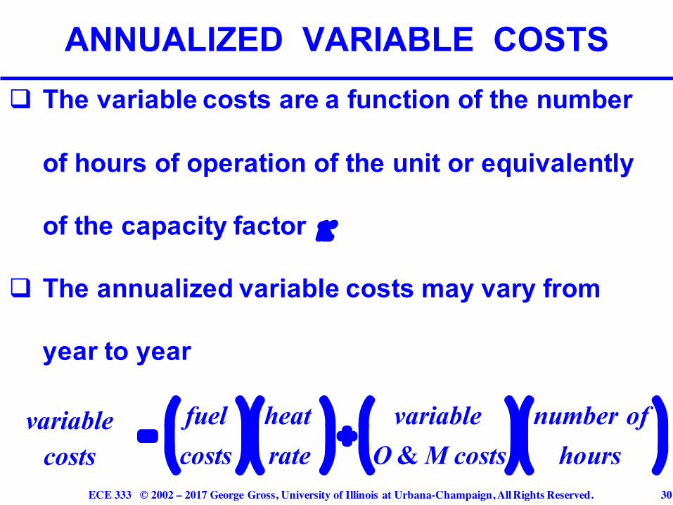
q The variable costs are a function of the number
of hours of operation of the unit or equivalently
of the capacity factor
q The annualized variable costs may vary from
year to year
ANNUALIZED VARIABLE COSTS
variablecosts
=fuelcosts
!
"#
$
%&
heatrate
!
"#
$
%& +
variableO & M costs
!
"#
$
%&
number ofhours
!
"#
$
%&
κ
ECE 333 © 2002 – 2017 George Gross, University of Illinois at Urbana-Champaign, All Rights Reserved. 31
q The yearly variable costs explicitly account for
fuel cost escalation
q Often, the yearly costs are given on a per unit – kW
or MW – basis
q We illustrate these concepts with a pulverized –
coal steam plant
ANNUALIZED VARIABLE COSTS
ECE 333 © 2002 – 2017 George Gross, University of Illinois at Urbana-Champaign, All Rights Reserved. 32
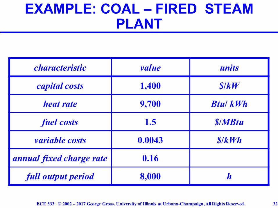
EXAMPLE: COAL – FIRED STEAM PLANT
characteristic value units
capital costs 1,400 $/kW
heat rate 9,700 Btu/ kWh
fuel costs 1.5 $/MBtu
variable costs 0.0043 $/kWh
annual fixed charge rate 0.16
full output period 8,000 h

ECE 333 © 2002 – 2017 George Gross, University of Illinois at Urbana-Champaign, All Rights Reserved. 33
q The annualized fixed costs per kW are
q The initial year annual variable costs per kW are
EXAMPLE: COAL–FIRED STEAM PLANT
1.5×10 −6 $ / Btu( ) 9,700 Btu / kWh( ) +0.0043 $ / kWh
#
$%%
&
'((
8,000h( )
= 150.8$ / kW
1,400 $ / kW( ) 0.16( ) = 224 $ / kW

ECE 333 © 2002 – 2017 George Gross, University of Illinois at Urbana-Champaign, All Rights Reserved. 34
q Total annual costs for 8,000 h are
q Note, we do the example under the assumption of full output for 8,000 h and 0 output for the
remaining 760 h of the yearq We also neglect any possible outages of the unit
and so explicitly ignore any uncertainty in the unit performance
EXAMPLE: COAL–FIRED STEAM PLANT
224 +150.8( )$ / kW8,000 h
= 0.0469 $ / kWh
Related Documents