• • •

Welcome message from author
This document is posted to help you gain knowledge. Please leave a comment to let me know what you think about it! Share it to your friends and learn new things together.
Transcript

Durham Research Online
Deposited in DRO:
04 January 2013
Version of attached le:
Other
Peer-review status of attached le:
Peer-reviewed
Citation for published item:
Sanchez, A.G. and Crocce, M. and Cabre, A. and Baugh, C.M. and Gaztanaga, E. (2009) 'Cosmologicalparameter constraints from SDSS luminous red galaxies: a new treatment of large-scale clustering.', Monthlynotices of the Royal Astronomical Society., 400 (3). pp. 1643-1664.
Further information on publisher's website:
http://dx.doi.org/10.1111/j.1365-2966.2009.15572.x
Publisher's copyright statement:
The denitive version is available at www.blackwell-synergy.com
Additional information:
Use policy
The full-text may be used and/or reproduced, and given to third parties in any format or medium, without prior permission or charge, forpersonal research or study, educational, or not-for-prot purposes provided that:
• a full bibliographic reference is made to the original source
• a link is made to the metadata record in DRO
• the full-text is not changed in any way
The full-text must not be sold in any format or medium without the formal permission of the copyright holders.
Please consult the full DRO policy for further details.
Durham University Library, Stockton Road, Durham DH1 3LY, United KingdomTel : +44 (0)191 334 3042 | Fax : +44 (0)191 334 2971
https://dro.dur.ac.uk

arX
iv:0
901.
2570
v4 [
astr
o-ph
.CO
] 1
9 A
ug 2
009
Mon. Not. R. Astron. Soc. 000, 000–000 (0000) Printed 19 August 2009 (MN LATEX style file v2.2)
Cosmological parameter constraints from SDSS luminous
red galaxies: a new treatment of large-scale clustering.
Ariel G. Sanchez1⋆, M. Crocce2, A. Cabre2, C. M. Baugh3 and E. Gaztanaga2
1 Max-Planck-Institut fur Extraterrestrische Physik, Giessenbachstrasse, 85748 Garching, Germany.2 Institut de Ciencies de l’Espai, CSIC/IEEC, Campus UAB, F. de Ciencies, Torre C5 par-2, Barcelona 08193, Spain.3 The Institute for Computational Cosmology, Department of Physics, University of Durham, South Road, Durham DH1 3LE, UK.
Submitted to MNRAS
ABSTRACT
We apply a new model for the spherically averaged correlation function at large pairseparations to the measurement of the clustering of luminous red galaxies (LRGs)made from the SDSS by Cabre & Gaztanaga (2009a). Our model takes into accountthe form of the BAO peak and the large scale shape of the correlation function. Weperform a Monte Carlo Markov chain analysis for different combinations of datasetsand for different parameter sets. When used in combination with a compilation of thelatest CMB measurements, the LRG clustering and the latest supernovae results giveconstraints on cosmological parameters which are comparable and in remarkably goodagreement, resolving the tension reported in some studies. The best fitting model inthe context of a flat, Λ-CDM cosmology is specified by Ωm = 0.261 ± 0.013, Ωb =0.044 ± 0.001, ns = 0.96 ± 0.01, H0 = 71.6 ± 1.2 kms−1 Mpc−1 and σ8 = 0.80 ± 0.02.If we allow the time-independent dark energy equation of state parameter to vary,we find results consistent with a cosmological constant at the 5% level using all datasets: wDE = −0.97 ± 0.05. The large scale structure measurements by themselvescan constrain the dark energy equation of state parameter to wDE = −1.05+0.16
−0.15,independently of CMB or supernovae data. We do not find convincing evidence for anevolving equation of state. We provide a set of “extended distance priors” that containthe most relevant information from the CMB power spectrum and the shape of theLRG correlation function which can be used to constrain dark energy models andspatial curvature. Our model should provide an accurate description of the clusteringeven in much larger, forthcoming surveys, such as those planned with NASA’s JDEMor ESA’s Euclid mission.
Key words: cosmological parameters, large scale structure of the universe
1 INTRODUCTION
The acoustic peaks imprinted on the temperature powerspectrum of the cosmic microwave background (CMB)have now been measured with impressive precision bya number of experiments (Lee et al. 2001; Bennet et al.2003; Hinshaw et al. 2003, 2007, 2009; Jones et al. 2006;Reichardt et al. 2009). These observations place tight con-straints on the values of many of the fundamental cosmo-logical parameters. With the fifth year of integration fromthe WMAP satellite there is seemingly little room left forany deviation from the basic ΛCDM model (Dunkley et al.2009; Komatsu et al. 2009). However, degeneracies exist be-
⋆ E-mail: [email protected]
tween some parameters which cannot be broken by CMBdata alone (e.g. (Bond et al. 1997; Efstathiou & Bond1999; Bridle et al. 2003). Perhaps the two most importantexamples are the curvature of the Universe and the equationof state of the dark energy, wDE = PDE/ρDE, where PDE isthe pressure of the dark energy and ρDE is its density. Mean-ingful constraints cannot be obtained on these parametersusing CMB data in isolation.
The full potential of the CMB measurements is real-ized when these data are combined with other observa-tions, such as the Hubble diagram of type Ia supernovaeand the large scale structure of the Universe as tracedby galaxies (Riess et al. 1998; Perlmutter et al. 1999;Efstathiou et al. 2002; Percival et al. 2002; Spergel et al.2003; Riess et al. 2004; Tegmark et al. 2004; Seljak et al.
c© 0000 RAS

2 A.G. Sanchez et al.
2005; Sanchez et al. 2006; Astier et al. 2006; Seljak et al.2006; Wang & Mukherjee 2006; Wood-Vasey et al. 2007;Spergel et al. 2007; Komatsu et al. 2009; Okumura et al.2008; Xia et al. 2008; Ferramacho et al. 2009). These com-plementary data sets come from the late Universe comparedwith the CMB data, and the interpretation of the observa-tions is more complicated and controversial.
Type Ia supernovae (SNe) have been proposed as stan-dard candles which can probe the luminosity distance - red-shift relation. The first strong evidence in support of a cos-mological constant came from combining the SNe data withCMB measurements (Riess et al. 1998; Perlmutter et al.1999). The type Ia Hubble diagram has come under in-tense scrutiny to uncover any hint of non-standardness aris-ing from the nature of the host galaxy, possible evolutionwith redshift or variation in dust extinction (Sullivan et al.2003; Gallagher et al. 2005; Ellis et al. 2008; Howell et al.2009). A recent joint analysis of SNe from different datasetssuggests that the systematic error on the equation of stateparameter from a joint CMB and SNe analysis is comparableto the size of the random error (Kowalski et al. 2008).
The power spectrum of galaxy clustering has also beenused in combination with CMB data (e.g. Percival et al.2002). According to the standard lore, the galaxy powerspectrum on large scales is expected to have a simple re-lation to the underlying dark matter spectrum. Moreover,the shape of the spectrum is believed to closely followthat expected in linear perturbation theory for the mat-ter, which can be readily computed given a set of valuesfor the cosmological parameters. However, with the avail-ability of improving measurements and more refined mod-elling of the galaxy power spectrum it has become clear thatthis simple picture is no longer sufficiently accurate to de-scribe the data. Additional levels of modelling of the devi-ations from linear theory have to be incorporated into theanalysis. These include empirical models of the nonlineardistortion of the power spectrum (Smith et al. 2003) andpossible scale dependent biases between the clustering ofgalaxies and mass (Cole et al. 2005; Hamann et al. 2008;Cresswell & Percival 2009). Recent studies have cast doubton the accuracy of these prescriptions (Sanchez & Cole2008; Reid et al. 2008). In principle, if the simple modelsdescribed the form of the observed power spectrum, thenthe power spectra measured from different galaxy samplesshould yield equivalent constraints on cosmological parame-ters. However, Sanchez & Cole (2008) found a fundamentaldifference in the shapes of the galaxy power spectra mea-sured from the two-degree galaxy redshift survey and theSloan Digital Sky Survey, after attempting to correct themeasured spectra. These authors found that the red selec-tion of the SDSS galaxies results in a strong scale dependentbias (see also Swanson et al. 2008). Similar scale dependenteffects have been seen in the power spectrum of dark matterhaloes and galaxies modelled in simulations (Smith et al.2007; Angulo et al. 2008).
Recent analyses have not attempted to model the over-all shape or amplitude of the power spectrum, as a conse-quence of the difficulties described above in interpreting theresults from different samples. Instead, attention has shiftedto a pattern of oscillatory features called the baryonic acous-tic oscillations (BAO), which are imprinted on the matterpower spectrum. These features have been advocated as a
standard ruler which can be used to measure the distance-redshift relation, and hence constrain the dark energy equa-tion of state (Blake & Glazebrook 2003; Hu & Haiman2003; Linder et al. 2003; Seo & Eisenstein 2003; Wang2006; Guzik et al. 2007; Seo & Eisenstein 2007; Seo et al.2008). The BAO arise from oscillations in the baryon-photon fluid prior to matter-radiation decoupling. This phe-nomenon gives rise to the peaks seen in the power spec-trum of temperature fluctuations in the CMB. In the mat-ter power spectrum, the oscillations have a much smalleramplitude as baryons only account for around 20 per centof the total matter density of the Universe. Furthermore,the oscillations in the matter spectrum are out of phasewith those in the CMB (Sugiyama 1995; Eisenstein & Hu1998, 1999; Meiksin et al. 1999). The oscillation scale isrelated to the size of the sound horizon at recombination,which can be measured with high accuracy from the CMB(Komatsu et al. 2009). The apparent size of the BAO rulerdepends upon the parameters wDE and Ωk, as these deter-mine the angular diameter distance out to a given redshift.In practice, the BAO are not precisely a standard ruler atthe level of precision demanded for their interpretation infuture surveys. Nevertheless, by modelling the appearanceof the BAO accurately, they are still a valuable probe ofcosmological parameters (Sanchez et al. 2008; Smith et al.2008). Careful simulation work and modelling has shownthat techniques can be developed which can overcome long-wavelength gradients in the power spectrum to yield robustconstraints on the BAO using the galaxy power spectrum(Percival et al. 2007b; Smith et al. 2007; Angulo et al.2008; Crocce & Scoccimarro 2008; Takahasi et al. 2008;Seo et al. 2008).
The BAO signal has been detected in both the 2dF-GRS and SDSS surveys (Cole et al. 2005; Eisenstein et al.2005). The most powerful BAO measurements currentlycome from samples of luminous red galaxies (LRGs)(Cole et al. 2005; Hutsi 2006; Padmanabhan et al.2007; Percival et al. 2007b,c; Okumura et al. 2008;Cabre & Gaztanaga 2009a; Gaztanaga et al. 2008b;Martinez et al. 2009). Detections at a lower significancehave also been reported using galaxy clusters (Hutsi 2007;Estrada et al. 2009). The imprint of these features haseven been found in the three point function of LRGs(Gaztanaga et al. 2008a). Despite this rapid progress, theconclusions drawn from measurements of the BAO remainunclear. For example, Percival et al. (2007c) analysedthe BAO signal in a joint galaxy sample drawn from theSloan Digital Sky Survey (SDSS) data release five (DR5)and the two-degree Field Galaxy Redshift Survey (2dF-GRS). Ignoring the information from the amplitude andlong-wavelength shape of the power spectrum, and simplyisolating the BAO, the results of Percival et al. showed a2.4σ discrepancy with the distance measurements inferredfrom the supernovae type Ia (SN) data by Astier et al.(2006), signaling a possible problem in the modelling of theBAO data, or a challenge to the ΛCDM model.
Much theoretical work has been devoted to uncover-ing scale dependent effects in the BAO and in improvingthe modelling of the signal in galaxy surveys (Angulo et al.2005; Huff et al. 2007; Smith et al. 2007; Angulo et al.2008; Smith et al. 2008; Crocce & Scoccimarro 2008;Seo et al. 2008; Desjacques 2008). In order to realize the
c© 0000 RAS, MNRAS 000, 000–000

Cosmological parameters from the SDSS-DR6 LRGs ξ(s) 3
full potential of the BAO technique as a cosmological probeit is essential to quantify any systematics in the signaland to understand how the measurements relate to cos-mological parameters. First, let us debunk some possiblepreconceptions about BAO. As we have remarked above,the BAO are not precisely a standard ruler. In the corre-lation function, the Fourier transform of the power spec-trum, the BAO appear as a broad peak at large pair sep-arations (Matsubara 2004). Sanchez et al. (2008) showedthat even in linear perturbation theory, the maximum of theBAO peak in correlation function does not coincide with thesound horizon scale at the percent level of accuracy requiredto fully exploit the measurements expected from forthcom-ing galaxy surveys. Furthermore, Smith et al. (2008) andCrocce & Scoccimarro (2008) have shown that both largevolume numerical simulations and theoretical predictionsbased on renormalized perturbation theory (RPT) indicatethat the BAO peak in the correlation function is shifted anddistorted in a non-trivial manner relative to the prediction oflinear perturbation theory. If unaccounted for, these shiftsbias the constraints obtained by using the BAO measure-ments as a standard ruler.
Careful modelling of the correlation function is thereforerequired to extract the cosmological information encoded inlarge scale structure. Sanchez et al. (2008) argued that thecorrelation function is less affected by scale dependent ef-fects than the power spectrum and that a simple model forthe correlation function proposed by Crocce & Scoccimarro(2008), based on RPT (Crocce & Scoccimarro 2006a,b),gives an essentially unbiased measurement of the dark en-ergy equation of state. This means that information fromthe large scale shape of the correlation function, in addi-tion to the form of the BAO peak, can be used to providerobust constraints on cosmological parameters. The correla-tion function therefore provides a better constraint on thedistance scale than the more conservative, “BAO only” ap-proach required when using the power spectrum (i.e. whichrequires the long wavelength shape information to be dis-carded along with the amplitude).
In this paper we apply this new model to theshape of the redshift space correlation function, ξ(s),of the SDSS Data release 6 (DR6) LRGs measured byCabre & Gaztanaga (2009a). The LRG sample analysedby Cabre & Gaztanaga (2009a) is twice the size of thesample used to make the first detection of the BAO byEisenstein et al. (2005), and has also yielded the first mea-surement of the radial BAO signal, which constrains theHubble parameter (Gaztanaga et al. 2008b). We combinethe LRG clustering information with the latest measure-ments of CMB and SNe data. We focus on the constraintson the dark energy equation of state and the curvature ofthe Universe, which are the parameters where the extra in-formation from the shape of ξ(s) can dramatically improveupon the CMB only constraints. We also pay special atten-tion to the consistency of the results obtained with differentdataset combinations.
The outline of the paper is as follows. In Section 2,we describe the data used in our parameter estimation. InSection 3 we describe the details of our modelling of theshape of the redshift space correlation function and com-pare it with measurements in N-body simulations. We alsoset out the different parameter spaces that we study and
describe our methodology for parameter estimation. In Sec-tion 4 we assess the impact of the details of the parameterestimation technique on the obtained constraints on cosmo-logical parameters. Section 5 presents our main results forthe parameter constraints obtained by comparing theoreti-cal models to the CMB data and the correlation function ofthe SDSS-DR6. In Section 6 we focus on the constraints oncertain distance combinations obtained from the shape ofξ(s). We summarize our conclusions in Section 7. AppendixA gives the theoretical motivation for the model we use todescribe the correlation function and Appendix B gives thecovariance matrix for the distance constraints.
2 THE DATASETS
Here we describe the different datasets that we use to con-strain cosmological parameters. The modelling of the cor-relation function of luminous red galaxies is described lateron in Section 3.2. The datasets described below are used indifferent combinations to check the consistency of the con-straints returned.
2.1 The redshift space correlation function of
SDSS-DR6 LRGs: the monopole
Luminous red galaxies (LRGs) are an efficient tracer of thelarge scale structure of the Universe. These galaxies are se-lected by color and magnitude cuts designed to identify in-trinsically red, bright galaxies using SDSS photometry (seeEisenstein et al 2001 for a complete description of the colorcuts). LRGs can be seen out to higher redshifts than galax-ies in a simple magnitude limited catalogue, and so mapa larger volume of the Universe. LRGs have a low spacedensity compared to L∗ galaxies, which means that fewerredshifts have to be measured to map out the same volume.The low space density, which translates into a higher shotnoise, is compensated for by the stronger than average clus-tering of LRGs, which maintains the signal-to-noise of thecorrelation function at a level which can be measured.
Here we use the measurement of the 2-point cor-relation function of LRGs in redshift space made byCabre & Gaztanaga (2009a) shown by the black points inFig. 1. These authors studied the clustering of LRGs inData Release 6 (DR6) of the Sloan Digital Sky Survey(SDSS), which has 75 000 LRG galaxies spanning a volumeof 1h−3 Gpc3 over the redshift interval 0.15 < z < 0.47. Thecomparison between DR6 and the result of Eisenstein et al.(2005) is plotted in Fig.B4 of Cabre & Gaztanaga (2009a)and Fig. 1; the two results are in good agreement with theDR6 result showing an improvement of a factor of about√
2 in the size of the errors. Cabre & Gaztanaga (2009a)carried out an extensive series of tests of their measurementof the LRG correlation function. They found that system-atic uncertainties in the estimation of the radial selectionhave a small impact on the results (ie see their figure B2).The adoption of different weighting schemes also producesnegligibly small changes (their Fig.B5 and B11). These care-ful tests indicate that this new estimation of the correlationfunction is robust and that any possible systematic effectsare small compared to the error bars.
Here we recap two aspects of the analysis of
c© 0000 RAS, MNRAS 000, 000–000

4 A.G. Sanchez et al.
Figure 1. The spherically averaged correlation function of LRGsin redshift space. Circles with errorbars show the correlation func-tion used in this paper. The shaded region shows the dispersionin the correlation function obtained when using the new MAN-GLE mask of Swanson et al. (2008) with different completenessfractions. The dotted line shows the result for the north stripeof DR6. We have also calculated the correlation function for thenew DR7 (solid line), estimated using a random catalog generatedfrom a smoothed version of the selection function. The dashed lineshows the estimate from DR7 without smoothing. The measure-ment from Eisenstein et al. (2005) is shown using triangles; notethese authors had fewer LRGs and used broader bins.
Cabre & Gaztanaga (2009a) which are particularly relevantto this paper: the treatment of the survey mask and the esti-mation of the covariance matrix of the correlation function.
An accurate knowledge of the angular and radial se-lection of a galaxy catalogue, including the redshift com-pleteness as a function of magnitude and position on thesky, is an essential prerequisite for a measurement of clus-tering. This information allows the mean density of galaxiesin the survey to be estimated. After the release of DR6,Swanson et al. (2008) provided this information in a read-ily usable form, translating the original mask files extractedfrom the NYU Value-Added Galaxy Catalog (Blanton et al.2005), from MANGLE into Healpix format (Gorski et al.1999). Cabre & Gaztanaga (2009a) describe how they con-structed a survey “mask” for LRGs and tested the impactof the mask on clustering measurements using mock cata-logues. Using the same techniques, we have also examinedthe correlation function of LRGs in DR7, which has be-come available since the submission of Cabre & Gaztanaga(2009a). In Fig. 1, we plot a summary of the possible sys-tematics in the estimation of the correlation function. Theestimates corresponding to different versions of the surveymask and different ways of generating a catalogue of randompoints are in remarkably good agreement with one another.Furthermore, the results from DR6 and DR7 are in excel-lent agreement; DR7 represents only a modest improvementover DR6. The results of Eisenstein et al. (2005) are plotted
in Fig. 1 using triangles. Their estimate is consistent withthat of Cabre & Gaztanaga (2009a) within the errors (notethat their binning is different, and also, perhaps, their nor-malisation, due to a small shift which could be attributedto systematics (see Section 2.1.1)). Whilst there is a mod-est improvement in the parameter constraints on using theDR7 measurement, in line with the incremental change inthe number of LRGs and the solid angle covered, we havedecided to retain the DR6 measurement in this paper, be-cause the survey mask has been tested more extensively inthat case. The DR6 measurement represents a factor of ∼ 2more volume than that covered by the LRG sample analyzedby Eisenstein et al. (2005).
Cabre & Gaztanaga (2009a) constructed a covariancematrix for the LRG correlation function using mock cata-logues drawn from the MareNostrum Institut de Ciencias delEspacio (MICE1) N-body simulations (Fosalba et al. 2008;Crocce et al. 2009). The extremely large volume of this run(box size 7680 h−1 Mpc) allowed 216 essentially indepen-dent LRG DR6 mocks to be extracted. Cabre & Gaztanaga(2009a) investigated different methods to estimate the erroron the correlation function (see their Appendix A). Theyfound that the jackknife error, an internal estimate madefrom the dataset itself (JK; see Norberg et al. 2008), gavea reasonable match to the diagonal elements of the covari-ance matrix obtained directly from the 216 mock catalogues.However, the JK estimate of the off-diagonal elements ofthe covariance matrix is noisier than that obtained fromthe mocks. In this analysis we construct the full covariancematrix of the measurement from the correlation matrix es-timated from mock catalogues of dark matter haloes withsimilar clustering and abundance to the LRGs, rescaled bythe JK estimate of the variance from the data, which has theadvantage of being independent of the cosmological modeladopted in the N-body simulation.
2.1.1 The implications of a possible constant systematic
shift in clustering amplitude
Small systematic effects including, for example, the integralconstraint, calibration errors or evolutionary effects, will, ifunaccounted for, appear as an additive term in the mea-sured correlation function: ξ(s) = ξtrue(s) + ξsys(s), whereξsys(s) stands for the systematic error. The simplest modelfor ξsys(s) is a constant shift, ξsys(s) = K, which we labelhere as the K-shift. Systematic shifts include both effectswhich are unaccounted for in the estimate of the radial selec-tion function and angular calibration errors which can movegalaxies in or out of the galaxy sample. These can introducespurious fluctuations in the observed density. A 1% varia-tion in (r − i) color or a 3% shift in r magnitude can intro-duce a 10% modulation in the LRG target number density(Eisenstein et al. 2001). However, Hogg et al. (2005) foundthat the large scale density variations in the final LRG sam-ple are completely consistent with the predictions of biasedΛCDM models, showing that when averaged over large an-gular scales, the fluctuations in the photometric calibrationof the SDSS do not affect significantly the uniformity of theLRG sample. Even a spurious number density fluctuation as
1 http://www.ice.cat/mice
c© 0000 RAS, MNRAS 000, 000–000

Cosmological parameters from the SDSS-DR6 LRGs ξ(s) 5
large as δ ∼ 5% can only produce a shift K = δ2 < 0.0025.As illustrated in Fig.1 the potential systematics that we areable to check seem to produce shifts of |K| < 0.001.
These are small changes, but could our analysis belowbe affected by such a systematic effect, if present? We havechecked this explicitly by repeating our analysis allowingfor a constant additive term K as an extra free parame-ter, which we marginalize over. We imposed a prior on thisK-shift as large as |K| = 0.01. This corresponds to 10%density fluctuations, well above the expected systematics inthe LRG sample. We find that even with this wide prior inK, the marginalization over the additive K-shift does notchange the obtained errors of the cosmological parametersand only changes the mean values by less than 0.5σ in themost extreme cases. This small difference does not justifythe inclusion of this extra parameter. But note that if wewant to address the question of what is the absolute good-ness of fit, then it might be important to consider such aK-shift as an additional degree of freedom. We will comeback to this question in Sec. 7.
2.2 The redshift space correlation function of
SDSS-DR6 LRGs: the radial BAO peak
The main piece of clustering information we shall use in thispaper is the monopole or spherical average of the two-pointredshift space correlation function described in the previoussubsection. However, there is also useful cosmological infor-mation in the form of the correlation function split into binsof pair separation parallel (π) and perpendicular (σ) to theline of sight, ξ(σ, π). Gaztanaga et al. (2008b) found a sig-nificant detection of a peak along the line-of-sight direction,the position and shape of which is consistent with it beingthe baryonic acoustic peak.
Gaztanaga et al. (2008b) measured the position of theradial BAO peak (rBAO) using the full LRG DR6 sample,and two sub-samples at low, z = 0.15 − 0.30, and high red-shifts, z = 0.40 − 0.47 (see their Table II). In this paperwe make use of these two last measurements, which can betreated as independent due to the large separation betweenthese redshift intervals. When combined with a measure-ment of the sound horizon scale from the CMB, the positionof the BAO feature can be used as a standard ruler to obtaina constraint on the value of the Hubble parameter, H(z), asa function of redshift (Gaztanaga et al. 2008b). Here, in-stead of calibrating the radial BAO distance rBAO(z) withthe CMB, we follow the same approach as Gaztanaga et al.(2008c) and use the measurement of the dimensionless red-shift scale
∆zBAO(z) = rBAO(z)Hfid(z)
c. (1)
In this equation Hfid(z) is the Hubble constant at theredshift of the measurement in the fiducial cosmology as-sumed by Gaztanaga et al. (2008b) to convert the observedgalaxy redshifts into comoving distances. Note that the fac-tor Hfid(z)/c in Eq. (1) ensures that ∆zBAO does not dependon the fiducial cosmology assumed to obtain the rBAO mea-surement. Section 3.3 describes the details of our modellingof these measurements.
Because of the narrow range of σ values (0.5 < σ <5.5 h−1 Mpc) used in the radial measurement, the rBAO re-
Figure 2. Normalized covariance matrix estimated from 216mocks LRG samples. Here we test the covariance between themonopole correlation (horizontal axis) and the radial (LOS) cor-relation (vertical axis). The correlation is only important on smallscales and is negligible (less than 10%) for the scales of interesthere (> 40 h−1 Mpc).
sults are essentially independent from the monopole of thetwo-point function; fewer than 1% of the bins considered inthe spherically averaged correlation function are used in theestimate of the radial correlation. For this reason we treatthese two datasets as independent. We tested this explicitlyusing the mock LRG catalogues from Cabre & Gaztanaga(2009a) (the same set used to estimate the covarince matrixin the monopole), to evaluate the covariance of the radialand the monopole correlations. Fig. 2 shows the normalizedcovariance:
Cij =1
M
MX
k=1
[ξm(i)k − bξm(i)]
σm(i)
[ξr(j)k − bξr(j)]
σr(j)(2)
where ξm(i)k and ξr(j)k are the monopole and radial cor-
relation in the i-th and j-th bins respectivelly measured inthe k-th mock catalogue (k = 1, ...M) and bξ and σ are thecorresponding mean and rms fluctuations over the M re-alizations. As shown in Fig.2 the covariance on the scalesof interest in our analysis (larger than 40 h−1 Mpc) is quitesmall (less than the noise in the estimation, of about 10%)which shows that the two datasets are indeed independentin practice. This implies that the rBAO measurements ob-tained from the radial correlation functions are independentfrom the monopole ξ(s).
2.3 CMB data: temperature and polarization
power spectra
The accuracy of recent observations of the CMB meanthat this is the single most powerful dataset for constrain-ing the values of cosmological parameters. The compila-tion of CMB measurements we use includes the tempera-ture power spectrum in the range 2 ≤ ℓ ≤ 1000 and thetemperature-polarization power spectrum for 2 ≤ ℓ ≤ 450of the first five years of observations of the WMAP satel-lite (Hinshaw et al. 2009; Nolta et al. 2009); the band-
c© 0000 RAS, MNRAS 000, 000–000

6 A.G. Sanchez et al.
power temperature spectrum from the 2008 observationsof the Arcminute Cosmology Bolometer Array Receiver(Kuo et al. 2007; Reichardt et al. 2009, ACBAR,) overthe spherical harmonic range 910 < ℓ < 1850; tempera-ture and polarization data from the Cosmic BackgroundImager (Readhead et al. 2004, CBI,) with 855 < ℓ <1700; observations from the 2003 flight of BOOMERANG(Ruhl et al. 2003; Jones et al. 2006; Montroy et al. 2006;Piacentini et al. 2006) in the range 925 < ℓ < 1400and the recent results for the temperature and polariza-tion power spectra measurements from QUaD (Ade et al.2008) over the range 893 < ℓ < 1864. These measurementsof the power spectrum of temperature fluctuations in theCMB cover the spherical harmonic range 2 < ℓ < 1800.Following Dunkley et al. (2009), in order to avoid cross-correlations with the WMAP data, we use only the band-powers of the small scale CMB experiments that do notoverlap with the signal-dominated WMAP data. Note thatthe QUaD measurements were not available at the time ofthe “WMAP+CMB” analysis carried out by Komatsu et al.(2008).
2.4 The Hubble diagram of type Ia supernovae
We also consider the constraints provided by the Hubblediagram of type Ia supernovae (SN) as provided by theUNION sample from (Kowalski et al. 2008). This compila-tion is drawn from 13 independent datasets processed usingthe SALT light curve fitter (Guy et al. 2005) and anal-ysed in a uniform way. The sample contains a set of 57low-redshift SN, the recent samples from the SuperNovaLegacy Survey (Astier et al. 2006, SNLS,) and the Equationof State SupErNovae trace Cosmic Expansion (ESSENCE,Miknaitis et al. 2007), the high-redshift sample from theHubble Space Telescope (Riess et al. 2004, 2007), as wellolder datasets (Riess et al. 1998; Perlmutter et al. 1999;Tonry et al. 2003; Barris et al. 2004). The final sample isthe largest available to date, comprising 307 SN which passthe selection criteria.
Kowalski et al. (2008) suggest a way to include the ef-fect of systematic errors when fitting the SN data. This es-timation and those from other authors (Astier et al. 2006;Wood-Vasey et al. 2007; Hicken et al. 2009), predict dif-ferent systematic errors in the estimated constraints on thedark energy equation of state, with values ranging from 5%to more than 10%. These approaches differ in the choice ofwhich potential sources of systematic errors are taken intoaccount and the estimation of their likely magnitude. It isour understanding that the community has not reached aconsensus about the correct way to estimate the effect of thesystematic errors in the analysis of the SN data. For this rea-son we follow other authors (e.g. Komatsu et al. 2009) anddo not include the systematic errors in our constraints oncosmological parameters. However, the inclusion of the sys-tematic errors in the SN data has important implications forthe derived values of the dark energy equation of state (seeSection 5.2). This should be borne in mind when compar-ing constraints obtained using SN data with those obtainedusing other datasets.
3 METHODOLOGY
In this section we summarize the approach used to obtainconstraints on cosmological parameters. We start by describ-ing he different parameter sets that we consider. The para-metric model we use to describe the shape of the correla-tion function in redshift space is presented 3.2. The the-oretical motivation for this parametric form can be foundin Appendix A. In Section 3.2, we also compare the modelwith measurements made using numerical simulations. Sec-tion 3.3 describes the model we implement to describe theradial BAO measurements. The methodology we follow toexplore and constrain the parameter spaces is discussed inSection 3.4.
3.1 The parameter space
In this paper we make the basic assumption that the primor-dial density fluctuations were adiabatic, Gaussian and hada power-law spectrum of Fourier amplitudes, with a negli-gible contribution from tensor modes. From the analysis ofthe fifth year of WMAP data, Komatsu et al. (2009) didnot detect any deviation from these hypotheses at the 99%confidence limit (CL). Within this framework, a cosmolog-ical model can be defined by specifying the values of thefollowing eight parameters:
P ≡ (Ωk, ωdm, ωb, τ, ns, As, Θ, wDE). (3)
We now go through the parameters in the above list, defin-ing each one and also explaining how the values of otherparameters are obtained, which we will refer to as derivedparameters.
The homogeneous background cosmology is describedthrough the various contributions to the mass-energy den-sity. These are, in units of the critical density: Ωk, whichdescribes the curvature of the universe; ωdm ≡ Ωdmh2, thedensity of the dark matter (assumed cold, where h is Hub-ble’s constant in units of 100 kms−1Mpc−1) and ωb ≡ Ωbh2,the baryon density. We assume that massive neutrinos makeno contribution to the mass budget. For most of this paper,we assume that the dark energy component has a constantequation of state independent of redshift, with the ratio ofpressure to density given by wDE. In section 5.3 we relaxthis assumption and analyse models allowing for a time vari-ation in this parameter. In this case we use the standard lin-ear parametrization given by (Chevallier & Polarski 2001;Linder et al. 2003)
wDE(a) = w0 + wa(1 − a), (4)
where a is the expansion factor and w0 and wa are parame-ters.
The form of the initial fluctuations is described by twoquantities; the scalar spectral index, ns and the primordialamplitude of the scalar fluctuations As. These parametervalues are quoted at the “pivot” scale wavenumber of k =0.05 Mpc−1.
We assume that the reionization of the neutral inter-galactic medium occurred instantaneously, with an opticaldepth given by τ . Finally, Θ gives the ratio of the sound hori-zon scale at the epoch of decoupling to the angular diameterdistance to the corresponding redshift.
c© 0000 RAS, MNRAS 000, 000–000
Cosmological parameters from the SDSS-DR6 LRGs ξ(s) 7
There are further basic quantities whose values can bederived from those listed in the set of Eq. (3):
Pderived ≡ (Ωm, h, ΩDE, σ8, zre, t0). (5)
The matter density parameter is given by Ωm = Ωdm + Ωb.The value of the Hubble constant is derived from h =p
(ωdm + ωb)/Ωm. The energy-density of the dark energyis set by ΩDE = 1 − Ωm − Ωk. The results for As can betranslated into a constraint on σ8, the rms linear pertur-bation theory variance in spheres of radius 8 h−1Mpc, us-ing the matter fluctuation transfer function. The redshiftof reionization, zre, can be computed from the values of τ ,the Hubble constant and the matter and baryon densities(Tegmark et al. 1994). The age of the universe is t0.
The ΛCDM cosmological model is the simplest modelwhich can account for the wide variety of cosmological ob-servations available today. This model is characterized bysix parameters:
P6
varied ≡ (ωdm, ωb, ns, τ, As, Θ), (6)
assuming Ωk = 0 and wDE = −1. This parameter space iswell constrained by the temperature and polarization powerspectrum measurements from five years of integration of theWMAP satellite (Komatsu et al. 2009). In Section 5.1 weanalyse the impact of the measurement of the shape of ξ(s)on the constraints in this parameter space.
Using the latest WMAP data, Komatsu et al. (2009)placed strong constraints on the possible deviations fromthe ΛCDM model, namely non-Gaussianity, the presence ofisocurvature modes, deviations from a pure power law scalarprimordial power spectrum, the presence of tensor modes,a non-negligible energy component in the form of massiveneutrinos and parity-violation interactions. However, thereare two parameters that signal important deviations of thestandard ΛCDM model that can not be tightly constrainedfrom CMB data alone: the curvature of the Universe Ωk andthe dark energy equation of state wDE. In order to assessthe improvement on the constraints once the informationon the shape of ξ(s) is included in the analysis, we explorefour parameter spaces which contain extensions of the simpleΛCDM set. First we extend the parameter set of Eq. (6) byadding a constant dark energy equation of state
P6+wDE
varied ≡ (ωdm, ωb, ns, τ, As, Θ, wDE), (7)
fixing Ωk = 0. The results obtained in this case are shownin Section 5.2.
In Section 5.3 we include the parametrization of Eq. (4)in our analysis and explore the extended parameter space
P6+w(a)varied ≡ (ωdm, ωb, ns, τ, As, Θ, w0, wa), (8)
where we also implement the hypothesis of a flat universewith Ωk = 0. We also analyse the effect of dropping thisassumption. First, in Section 5.4, we include Ωk as a freeparameter, with
P6+Ωk
varied ≡ (ωdm, ωb, ns, τ, As, Θ, Ωk), (9)
assuming that the dark energy is given by a cosmologicalconstant (or vacuum energy) with wDE = −1. Finally, inSection 5.5, we also allow this parameter to vary freely andwe explore the full parameter space of Eq. (3).
3.2 A physically motivated model for the
correlation function
In the linear perturbation theory regime (valid when thefluctuation amplitude is small, for instance at high redshiftor on very large scales), the shape of the matter correlationfunction is well understood and can be readily obtained us-ing linear Boltzmann solvers, such as CAMB (Lewis et al.2000). The shape of the correlation function, in the con-text of a standard adiabatic CDM model, is sensitive tothe values of the matter density, Ωmh2, the baryon densityΩbh
2, the spectral tilt ns and the density parameter of mas-sive neutrinos. The evolution with redshift of the correlationfunction is well understood in the linear regime. In this case,each Fourier mode of the density field evolves independentlyof the others and the shape of ξ is unaltered, although theoverall amplitude changes with time.
Unfortunately this simple behaviour is modified by anumber of nonlinear phenomena, which affect different scalesat different epochs. These include nonlinear effects gener-ated by the latter stages of gravitational instability, redshift-space distortions caused by gravitationally induced motionsand a possible non-trivial scale dependent bias relation be-tween the distribution of galaxies and the underlying darkmatter field (see, for example, the step-by-step illustration ofthese effects given by Angulo et al. 2008). Nonlinear growthresults in cross-talk between different Fourier modes and in-troduces scale dependent patterns in the clustering, even onlarge scales. This is particularly noticeable in the appear-ance of the BAO bump, which is sensitive to the match be-tween the amplitude and phases of the fluctuations aroundthe peak scale. Due to the distortion of the Fourier modesfrom their original values, nonlinear growth causes the BAObump to become smeared out and also to lose contrast. Sucheffects cannot be ignored when modelling low-redshift data.
On large scales, (r > 30h−1 Mpc), the correlation func-tion falls sharply with increasing comoving pair separation,scaling roughly as a power law ∼ r−γ , with γ ∼ 2.5. At evenlarger separations, this behaviour is altered by the emer-gence of a bump known as the BAO peak (e.g. see Fig. 3).This feature, first measured for LRGs by Eisenstein et al.(2005), is centered at about 110 h−1 Mpc and has a width of∼ 20h−1 Mpc. The amplitude of the peak in the LRG corre-lation function corresponds to a ∼ 1% excess in the numberof LRG pairs above the number expected in a random dis-tribution (e.g. Cabre & Gaztanaga 2009a).
To model the shape of the correlation function onlarge scales, we follow Crocce & Scoccimarro (2008) andSanchez et al. (2008) and adopt the following parametriza-tion:
ξNL(r) = b2ξL(r) ⊗ e−(k⋆r)2 + AMC ξ′L(r) ξ(1)L (r), (10)
where b, k⋆ and AMC are nuisance parameters, and the sym-bol ⊗ denotes a convolution. Here ξ′L is the derivative of thelinear correlation function and ξ
(1)L (r) is defined by the in-
tegral:
ξ(1)L (r) ≡ r · ∇−1ξL(r) = 4π
Z
PL(k) j1(kr)k dk, (11)
with j1(y) denoting the spherical Bessel function of or-der one. The model in Eq. 10 is primarily motivated byRPT, where the matter power spectrum is written as P =G2PL + PMC , with G a nonlinear growth factor and PMC
c© 0000 RAS, MNRAS 000, 000–000

8 A.G. Sanchez et al.
Figure 3. The correlation function of dark matter halos in red-shift space measured in an ensemble of 50 large-volume N-bodysimulations (with total volume of ∼ 105 h−3 Gpc3). The errorbars correspond to the error on the mean of the ensemble and areobtained from the scatter among the 50 realizations. The best fit-ting parametric model used in this work, Eq. (10), is shown by thesolid blue line (note the fit takes into account the covariance be-tween the bins). The dashed line corresponds to setting AMC = 0and highlights the importance of this term in matching the shapeof the correlation function at r < 80 h−1 Mpc. The scaling usesrBAO = 102h−1Mpc.
being the power generated by mode-coupling. To a verygood approximation G is of Gaussian form, while at largescales the leading order contribution of PMC in real spaceis ∼ ξ
(1)L ξ′L (see Appendix A for a detailed discussion).
The Gaussian degradation of the BAO information was alsoshown to be a good description by Eisenstein et al. (2006).
We now demonstrate how accurately the model ofEq. (10) can reproduce the spatial clustering of halo sam-ples with comoving number densities similar to that of theLRGs in DR6. To this end we utilize an ensemble of 50 re-alizations of collisionless dark matter N-body simulations.Each simulation contains 6403 particles in a comoving vol-ume V = L3 = (1280 h−1 Mpc)3. The cosmological param-eters were set to Ωm = 0.27, ΩΛ = 0.7, Ωb = 0.046 andh = 0.72. The initial power spectrum had spectral indexns = 1 and was normalized to give σ8 = 0.9 when lin-early extrapolated to z = 0. Halos were identified usingthe friends-of-friends algorithm with linking-length param-eter l = 0.2 (see Smith et al. 2008; Crocce & Scoccimarro2008, for more details).
Fig. 3 shows the 2-point correlation function measuredin redshift-space at z = 0 for two non-overlapping samplesof dark matter haloes of masses 7 × 10¹³ < M [h−1 M⊙] <15×1013 and 15×1013 < M [h−1 M⊙] (with number densitiesn[h3 Mpc−3] = 1.88 × 10⁻⁵ and 3.46 × 10⁻⁵ respectively).Our redshift space measurements were done considering thecontribution of peculiar velocities along one dimension in thesimulation (i.e. recreating a plane-parallel configuration).
Szapudi (2004) discussed in depth the issue of wideangle redshift space distortions. He found that openingangles θ . 15 − 20 would ensure the validity of theplane-parallel approximation. For the redshift range of theLRG sample considered in our analysis (0.15 < z < 0.47)and the largest pair-distance separation allowed (smax =150 h−1Mpc), the maximum opening angle is given bysin(θmax) = smax/DA(z = 0.15), which implies θmax ≈ 20.For the mean redshift of the sample the angle subtended bysmax is θ ≈ 10, well within the validity of the plane-parallelapproximation.
The error bars plotted show the error on the mean ob-tained from the ensemble of 50 simulations. Each simulationhas a larger volume than the LRG sample we use from DR6.Therefore these errors are ≈
√2 ×
√50 = 10 times smaller
than they would be for the LRG sample. This means thatthe deviations between models (solid lines) and simulationresults (points) are not important for our purposes.
The parametrization given in Eq. (10) corresponds tothe solid blue line in Fig. 3. The corresponding best-fit χ2
values for the nuisance parameters (k⋆[h Mpc−1], b, AMC)were (0.142, 1.94, 3.23) and (0.146, 2.75, 4.53) respectively.Clearly, the model can accurately describe the clusteringof halos in redshift space.
Sanchez et al. (2008) also compared Eq. (10) againstmeasurements of the non-linear correlation function froma similar large ensemble of N-body simulations at variousredshifts, and confirmed that this form gives an essentiallyunbiased measurement of the dark energy equation of stateusing both, real and redshift space information.
The dashed line in Fig. 3 corresponds to Eq. (10) withAMC = 0. From the plot we can see that the inclusion of thisterm is the key to recovering the correct clustering shapeat separations smaller than the BAO bump. In addition itcontributes slightly to the shape of the bump and alleviatesa systematic effect related to the position of the BAO peak(Crocce & Scoccimarro 2008) (but this is sub-dominant forthe survey volume being considered). In subsequent sectionswe check that this nuisance parameter is not degenerate withany of the cosmological parameters.
On theoretical grounds, one expects the smoothinglength k−1
⋆ to depend on cosmology (i.e. aside from galaxytype or redshift) with, for example, a 10% increase in Ωm ex-pected to increase k⋆ by about 4% (Crocce & Scoccimarro2006b; Matsubara 2008). In view of this, we decided to con-sider k⋆ as a nuisance parameter at the expense of a possibleincrease in error bars. Note that this is at variance with theapproach of Eisenstein et al. (2005), Tegmark et al. (2006)and Percival et al. (2007c) who kept this length fixed.
In summary, for each cosmological model we computethe linear correlation function ξL(r) using CAMB to gener-ate the corresponding transfer function, and simulate non-linear effects through Eq. (10) after computing ξ′L(r) and
ξ(1)L (r) from Eq. (11).
3.3 A model for the radial acoustic scale
Here we describe the simple model that we use to computethe dimensionless redshift radial acoustic scale ∆zBAO for agiven choice of the cosmological parameters of Eq. (3).
The value of ∆zBAO can be computed as,
c© 0000 RAS, MNRAS 000, 000–000

Cosmological parameters from the SDSS-DR6 LRGs ξ(s) 9
Table 1. The parameter space probed in our analysis. We assumea flat prior in each case. The parameter spaces that we considerare set out in Section 3.1.
Parameter Allowed range
ωdm 0.01 – 0.99ωb 0.005 – 0.1Θ 0.5 – 10τ 0 – 0.8ns 0.5 – 1.5
ln(1010As) 2.7 – 4.0wDE −2. – 0
Ωk −0.3 – 0.3
∆zBAO(z) =H(z)rs(zd)
c, (12)
where H(z) is the Hubble constant at the mean redshift ofthe measurements (zm = 0.24 and 0.43), and rs(zd) is thecomoving sound horizon at the drag epoch, which is givenby
rs(z) =c√3
Z (1+z)−1
0
da
a2H(a)√
1 + Ra, (13)
where R = 3Ωb/4Ωγ and Ωγ = 2.469× 10⁻⁵ h−2 for a CMBtemperature TCMB = 2.725 K. The value of zd can be com-puted with high accuracy from the values of ωb and ωdm
using the fitting formulae of Eisenstein & Hu (1998).The radial BAO scale measurements can be used to
place constraints on cosmological parameters independentlyof other datasets. Being a purely geometrical test, as in thecase of the SN data, the radial BAO measurements are notsensitive to all the cosmological parameters of Eq. (3) sincethey contain no information about the primordial spectrumof density fluctuations, that is As and ns, and of the opticaldepth to the last scattering surface τ .
3.4 Practical issues when constraining parameters
We use a Bayesian approach and explore the different pa-rameter spaces defined in Section 3.1 using the MarkovChain Monte Carlo (MCMC) technique. Our results weregenerated with the publicly available CosmoMC code ofLewis & Bridle (2002). CosmoMC uses the camb packageto compute power spectra for the CMB and matter fluctua-tions (Lewis, Challinor & Lasenby 2000). We use a general-ized version of camb which supports a time-dependent darkenergy equation of state (Fang et al. 2008). For each pa-rameter set considered, we ran twelve separate chains whichwere stopped when the Gelman and Rubin (1992) criteriareached R < 1.02. We implemented flat priors on our baseparameters. Table 1 summarizes the ranges considered fordifferent cosmological parameters in the cases where theirvalues are allowed to vary.
In order to establish the link between a given cosmo-logical model and the datasets described in Section 2 it isnecessary to include a small set of extra parameters givenby
Figure 4. The impact of a mismatch in cosmology on the formof the correlation function. The upper panel shows the differencebetween the correlation functions measured assuming differentfiducial cosmologies (ΛCDM models with varying Ωm) from thatobtained assuming Ωm = 0.25. The lower panel shows the samecomparison after applying the scale shift of Eq. (15) to take intoaccount the change in the value of Ωm.
Pextra ≡ (b, k⋆, AMC, ASZ), (14)
to the parameter sets described in Section 3.1. The biasfactor b, describes the difference in amplitude between thegalaxy correlation function and that of the underlying darkmatter. The values of k⋆ and AMC from Eq. (10) are alsoincluded as free parameters in our parameter space. ASZ
gives the amplitude of the contribution from the Sunyaev-Zeldovich effect to the CMB angular power spectrum onsmall scales (high ℓ). When quoting constraints on the pa-rameters of Eq. (3) and (5), the values of these extra pa-rameters are marginalized over. In the case of b, this is doneusing the analytic expression given in Appendix F of Lewis& Bridle (2002), but the remaining parameters are includedin our Monte Carlo analysis (see Section 3.4).
There is one important point that must be consideredin order to make a comparison between the model of Eq.(10)and the observational data of the LRG redshift-space cor-relation function. When measuring ξ(s), in order to mapthe observed galaxy redshifts and angular positions on thesky into distances, it is necessary to assume a fiducial cos-mological model. This choice has an impact on the resultsobtained.
One possible way to deal with this is to re-compute thecorrelation function and its covariance matrix for the cos-mology corresponding to each point in the Markov chains,and then use this measurement when computing the likeli-hood of the given cosmological model. This approach is in-feasible since it would require an exceedingly large amount ofcomputing time. Instead we follow an alternative approachby indirectly including the effect of the choice of the cosmol-ogy on the model correlation function. To do this we follow
c© 0000 RAS, MNRAS 000, 000–000

10 A.G. Sanchez et al.
Eisenstein et al. (2005) and simply rescale the distances inthe model correlation function by a factor
α =Dmodel
V
DfiducialV
, (15)
where the effective distance DV(zm) to the mean redshift ofthe survey zm = 0.35, is computed for each model as
DV(zm) =
»
D2A(zm)
cz
H(zm)
–1/3
. (16)
where DA(z) is the comoving angular diameter distancegiven by
DA(z) =c
H0
p
|Ωk|fk
„
H0
p
|Ωk|Z z
0
dz′
H(z′)
«
, (17)
where
fk(x) =
8
<
:
sinh(x) if(Ωk > 0),x if(Ωk = 0),sin(x) if(Ωk < 0).
(18)
The exponents within the square bracket on the right-hand side of Eq. (16) assume that the survey covers a widesolid angle, rather than a pencil-beam.
We can test the effectiveness of the correction factorgiven by Eq. (15) by applying it to different estimates of thecorrelation function computed with varying choices of thefiducial cosmology. Cabre & Gaztanaga (2009a) computedthe redshift space correlation function of SDSS-DR6 LRGsassuming different flat fiducial cosmologies with values ofΩm ranging from 0.2 to 0.3. The upper panel of Fig. 4 showsthe difference of these estimates from the one obtained forΩm = 0.25. It is clear that the choice of the cosmologicalmodel affects the shape of the correlation function. The ef-fect of this choice is particularly important on small scales(r < 70h−1 Mpc), but also introduces a small distortionto the shape of the acoustic peak, shifting its position to-wards larger (smaller) scales for smaller (larger) values ofΩm. If unaccounted for, this difference would bias the con-straints obtained on the cosmological parameters. The lowerpanel shows the same quantity once the correction factor ofEq. (15) has been applied. Clearly, this simple correctionis able to account for the choice of the fiducial cosmolog-ical model. We use this correction factor to translate themodel correlation function to the fiducial cosmology usedby Cabre & Gaztanaga (2009a) to estimate the LRG ξ(s)(a flat ΛCDM mode with Ωm = 0.25). We then computethe likelihood of the model assuming the Gaussian formL ∝ exp(−χ2/2).
4 TESTING THE MODEL OF ξ(S)
In this section we analyse the sensitivity of the parameterconstraints to the details of the procedure we follow to com-pute the likelihood of a given model. For the purpose of thisexercise we use the information contained in the correla-tion function of LRGs combined with the latest results fromthe WMAP satellite alone to constrain the parameter setof Eq. (7), and assess the impact on the results of varyingchoices in our analysis procedure.
First we study the sensitivity of the results to the rangeof scales in ξ(s) included in the analysis. Sanchez et al.
Figure 5. The dependence of the constraints on cosmologicalparameters on the minimum pair separation, rmin, included inthe correlation function measurement. The points show the meanvalue of the likelihood for each parameter and the error bars showthe 68% CL.
(2008) showed that the model of Eq. (10) gives an accu-rate description of the redshift-space halo correlation func-tion measured from N-body simulations on scales in therange 60h−1 Mpc ≤ r ≤ 180 h−1Mpc. In Section 3.2, weshowed that the second term in Eq. (10) also helps to re-produce the results from N-body simulations down to scalesof 40 h−1Mpc. Even though our measurement of ξ(s) ex-tends to larger scales, the measurement beyond 150 h−1 Mpcis noisy and does not have any effect on the constraints.Besides, Cabre & Gaztanaga (2009a) showed that on theselarge scales, the measurement of the redshift space correla-tion function exhibits an excess in the amplitude with re-spect to the previous estimate of Eisenstein et al. (2005).For this reason we have chosen to set a maximum distancermax = 150 h−1 Mpc in all subsequent analyses.
Fig. 5 shows the one-dimensional marginalized con-straints on a subset of the parameters space of Eq. (7) as afunction of the minimum scale, rmin, included in the analy-sis. For rmin < 40 h−1 Mpc we see that the constraints startto vary with rmin. Coincidentally, in this regime the modelof Eq. (10) starts to deviate from the N-body measurementsof the correlation function discussed in Sec. 3.2. On suchscales, extra terms beyond the one-loop contribution ∼ ξ′
c© 0000 RAS, MNRAS 000, 000–000

Cosmological parameters from the SDSS-DR6 LRGs ξ(s) 11
Table 2. The marginalized 68% interval constraints on the cosmological parameters of the ΛCDM model obtained using differentcombinations of the datasets described in Section 2, as stated in the column headings.
CMB CMB + ξ(s) CMB + rBAO CMB + SNCMB + ξ(s) CMB + ξ(s)
ξ(s)+ rBAO+ rBAO + rBAO + SN
100Θ 1.0416+0.0023−0.0023 1.0415+0.0022
−0.0022 1.0413+0.0022−0.0022 1.0413+0.0022
−0.0022 1.0414+0.0022−0.0022 1.0412+0.0022
−0.0022 0.987+0.065−0.069
ωdm 0.1091+0.0053−0.0053 0.1076+0.0038
−0.0038 0.1108+0.0036−0.0036 0.1125+0.0038
−0.0038 0.1095+0.0032−0.0032 0.1110+0.0029
−0.0029 0.091+0.040−0.038
100 ωb 2.282+0.050−0.051 2.280+0.050
−0.051 2.277+0.051−0.050 2.270+0.051
−0.051 2.276+0.049−0.049 2.267+0.050
−0.051 3.0+2.0−1.7
τ 0.088+0.016−0.016 0.090+0.017
−0.017 0.088+0.016−0.016 0.087+0.016
−0.016 0.088+0.016−0.016 0.086+0.016
−0.016 -
ns 0.965+0.013−0.013 0.965+0.012
−0.012 0.962+0.012−0.012 0.960+0.012
−0.012 0.963+0.011−0.011 0.960+0.011
−0.011 1.06+0.34−0.31
ln(1010As) 3.066+0.037−0.037 3.059+0.038
−0.038 3.067+0.036−0.036 3.070+0.036
−0.036 3.062+0.036−0.036 3.065+0.036
−0.036 -
ΩDE 0.749+0.026−0.026 0.755+0.018
−0.018 0.740+0.017−0.017 0.730+0.019
−0.020 0.747+0.014−0.014 0.739+0.013
−0.013 0.782+0.040−0.041
Ωm 0.251+0.026−0.026 0.244+0.018
−0.018 0.260+0.017−0.017 0.270+0.020
−0.019 0.253+0.014−0.014 0.261+0.013
−0.013 0.218+0.041−0.040
σ8 0.795+0.028−0.029 0.787+0.024
−0.024 0.802+0.024−0.024 0.810+0.023
−0.023 0.795+0.021−0.022 0.802+0.021
−0.021 -
t0/Gyr 13.64+0.11−0.11 13.64+0.10
−0.10 13.668+0.099−0.097 13.69+0.10
−0.10 13.660+0.097−0.096 13.682+0.095
−0.094 14.4+3.2−2.9
zre 10.5+1.3−1.3 10.5+1.3
−1.3 10.4+1.4−1.3 10.4+1.3
−1.3 10.4+1.3−1.3 10.4+1.3
−1.3 -
h 0.726+0.025−0.024 0.731+0.018
−0.018 0.718+0.016−0.016 0.710+0.017
−0.018 0.723+0.013−0.013 0.716+0.012
−0.012 0.73+0.15−0.14
to ξMC are expected to become important, which impliesthe breakdown of our ansatz.
For rmin > 40 h−1 Mpc, Fig. 5 shows that the con-straints on the values of the cosmological parameters arevery stable. Furthermore, the mean values obtained for theseparameters using CMB data plus the LRG correlation func-tion are in complete agreement with the ones obtained fromCMB information only. The allowed regions of some parame-ters, like ωb or ns which are tightly constrained by the CMBdata alone show almost no change on varying rmin. Otherparameters, such as Ωm or wDE show a substantial increasein their allowed regions as the data from small scales is grad-ually excluded from the analysis. For rmin = 42.5 h−1 Mpcwe obtain a constraint on the dark energy equation of stateof wDE = −0.996+0.097
−0.095 , while for rmin = 82.5 h−1 Mpc, thatis including only scales close to the acoustic peak in ξ(s),we get wDE = −0.99+0.17
−0.19 . This approximately factor of twochange in the error bar highlights the importance of theinclusion of information from the shape of ξ(s) on interme-diate scales. Based on this comparison and the results ofSection 3.2, we have chosen to set rmin = 42.5 h−1 Mpc inthe subsequent analysis.
We also studied the impact of the correction to the mea-sured correlation function to take into account changing thefiducial cosmology assumed when estimating ξ(s). For thistest we obtained constraints in the same parameter spacewithout applying the correction of Eq. (15). The results ob-tained in this way are entirely consistent with those obtainedwhen this correction is applied. The mean values of all theparameters remain practically identical with the exceptionof Ωm which shows a slight shift towards higher values ofapproximately 0.2σ. The allowed regions for these parame-ters also show almost no variation with a slight increase inthe confidence limits of Ωm and wDE of approximately 0.3σ.A similar shift but towards smaller values of Ωm is obtainedon setting AMC = 0 in the second term of the right handside of Eq. (10). This is in agreement with the results ofSanchez et al. (2008), who found that the two most impor-
tant parameters of this parametrization required to obtaina good description of the shape of the two-point correlationfunction are k⋆ and b (which in this case is marginalizedover).
In Section 5 we also present constraints obtained fromthe combination of the two large scale structure datasets weuse in our analysis, the LRG ξ(s) and the position of theradial acoustic peak, without including any CMB informa-tion. The fact that the correction for the fiducial cosmologydoes not significantly change the obtained results when theLRG ξ(s) is used in combination with the CMB, is not dueto the later keeping the constraints sufficiently close to thefiducial cosmology. As we will see later (see Section 5.2) theconstraints in this parameter space from CMB data alonepresent a strong degeneracy between Ωm and wDE, allowingfor models that differ substantially from our fiducial cosmol-ogy of Ωm = 0.25 and wDE = −1. Nonetheless, these modelsare ruled out by the ξ(s) data itself, (which on large scalesis insensitive to this correction), since the position of theacoustic peak shows a strong variation in these models. Theonly region of the parameter space allowed by the data isthat where the effect of the correction of Eq. (15) is small(although not completely negligible). This is the reason whythe obtained constrains are not extremely sensitive to thiscorrection. This also implies that this correction should notbe too important even in the case in which the LRG ξ(s)is combined with the radial acoustic peak whitout includingany CMB data. We have tested this explicitly and foundthat the resulting mean values of the cosmological param-eters obtained for this dataset combination when this cor-rection is not applied show no variation with respect to theones obtained when it is used. The only effect of ignoringthis correction is a small artificial increase of the allowedregions of Ωm and wDE of the same order as in the previouscase. Setting AMC = 0 for this combination of datasets alsoproduces a small shift towards smaller values of Ωm, whichin this case is much smaller than the allowed region for this
c© 0000 RAS, MNRAS 000, 000–000
12 A.G. Sanchez et al.
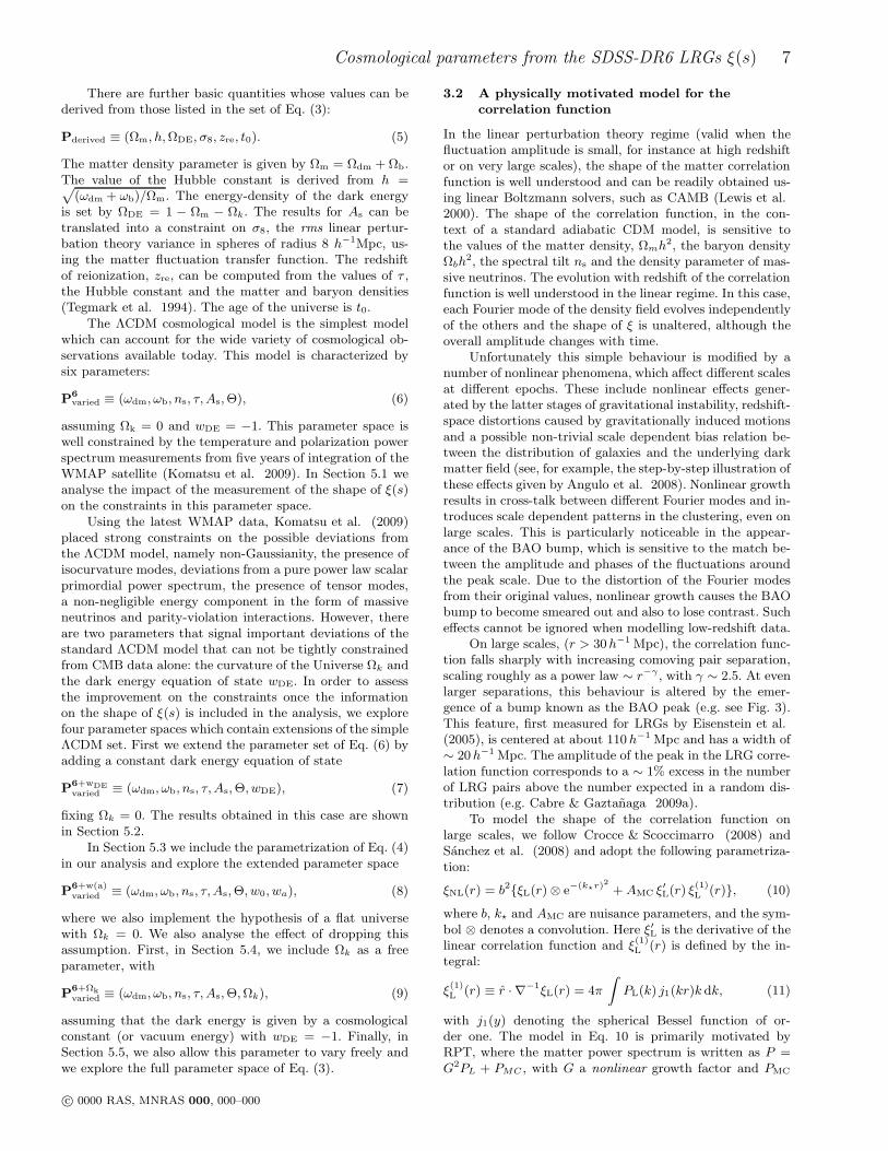
Figure 6. The marginalized, one-dimensional posterior likelihood in the ΛCDM parameter space (Eq. 6) obtained from CMB informationonly (dashed lines), CMB plus the shape of ξ(s) (solid line) and the full constraints including also rBAO and SN data (dot-dashed lines).
parameter. These tests show that our constraints are robustwith respect to the details of our analysis technique.
5 CONSTRAINTS ON COSMOLOGICAL
PARAMETERS
In this section, we carry out a systematic study of the con-straints placed on the values of the cosmological parametersfor the different parameter spaces defined in Section 3.4. InSection 5.1, we present the results for the simple ΛCDMcosmological model with six free parameters. In Section 5.2,we consider an extension to this parameter set, allowing thedark energy equation of state wDE to float (but without anyredshift dependence). Section 5.3 gives the constraints onmodels where the time variation of wDE is parametrized ac-cording to Eq. (4). In Section 5.4 we discuss our constraintson non-flat models, analysing the parameter space of Eq. (9).Finally, Section 5.5 shows the constraints on the full param-eter space of Eq. (3), allowing both for non-flat models andmore general dark energy models. Tables 2-6 compare theconstraints obtained in these parameter spaces using differ-ent combinations of the datasets described in Section 2.
5.1 The basic ΛCDM model
Due to the successful reproduction of a wide variety of obser-vations, the ΛCDM model has emerged over the past decadeas the new standard cosmological model. The recent resultsfrom five years of observations by the WMAP satellite havehelped to reinforce this conclusion. The latest WMAP datagive a much better estimation of the third acoustic peak inthe CMB temperature power spectrum, as well as the low-ℓ polarization signal. Thanks to these improvements, theWMAP data alone has been able to provide much tighterconstraints on this basic cosmological model than was pos-sible when using earlier releases.
Table 2 summarizes the constraints on the parametersof this simple model for different combinations of datasets.Fig. 6 shows the marginalized likelihoods for this param-eter set obtained using CMB data alone (dashed lines),CMB plus the LRG ξ(s) (solid lines) and the full combina-tion of the datasets described in Section 2 i.e. CMB+ LRGξ(s)+rBAO+SN (dot-dashed line). Several parameters, suchas ωb, ωc and τ , are tightly constrained by the CMB dataalone, and show almost no variation when other datasets areincluded in the analysis. On the other hand, the constraintson the parameters of the energy budget do show a markedimprovement on adding further datasets.
The CMB data is particularly sensitive to the value of
c© 0000 RAS, MNRAS 000, 000–000

Cosmological parameters from the SDSS-DR6 LRGs ξ(s) 13
Table 3. The marginalized 68% interval constraints on cosmological parameters allowing for variations in the (redshift independent)dark energy equation of state (i.e. the parameter set defined by Eq.(7)), obtained using different combinations of the datasets describedin Section 2, as stated in the column headings.
CMB CMB + ξ(s) CMB + rBAO CMB + SNCMB + ξ(s) CMB + ξ(s)
ξ(s)+ rBAO+ rBAO + rBAO + SN
wDE −0.73+0.30−0.30 −0.988+0.088
−0.088 −0.92+0.15−0.15 −0.950+0.054
−0.055 −0.999+0.090−0.091 −0.969+0.052
−0.052 −1.05+0.16−0.15
100Θ 10413+0.0023−0.0024 1.0415+0.0023
−0.0023 1.0414+0.0022−0.0022 1.0413+0.0023
−0.0022 1.0413+0.0023−0.0023 1.0414+0.0022
−0.0022 0.994+0.071−0.075
ωdm 0.1105+0.0052−0.0050 0.1068+0.0049
−0.0048 0.1095+0.0045−0.0045 0.10933+0.0049
−0.0050 0.1092+0.0042−0.0042 0.1088+0.0040
−0.0041 0.099+0.049−0.045
100 ωb 2.266+0.053−0.052 2.280+0.052
−0.052 2.277+0.051−0.051 2.272+0.052
−0.052 2.275+0.00051−0.049 2.275+0.051
−0.050 3.0+1.8−1.7
τ 0.089+0.017−0.017 0.090+0.017
−0.017 0.090+0.017−0.017 0.089+0.017
−0.017 0.088+0.017−0.017 0.088+0.016
−0.016 -
ns 0.959+0.014−0.014 0.965+0.012
−0.013 0.963+0.012−0.012 0.961+0.013
−0.013 0.963+0.011−0.012 0.963+0.012
−0.012 1.03+0.37−0.32
ln(1010As) 3.067+0.038−0.037 3.057+0.037
−0.037 3.066+0.037−0.037 3.064+0.038
−0.037 3.062+0.035−0.036 3.060+0.036
−0.036 -
ΩDE 0.63+0.12−0.12 0.754+0.020
−0.021 0.723+0.034−0.034 0.733+0.018
−0.019 0.746+0.017−0.017 0.739+0.013
−0.013 0.778+0.045−0.045
Ωm 0.36+0.12−0.12 0.245+0.021
−0.020 0.277+0.034−0.034 0.267+0.019
−0.018 0.254+0.017−0.017 0.261+0.013
−0.013 0.222+0.045−0.045
σ8 0.724+0.087−0.085 0.778+0.045
−0.045 0.774+0.060−0.060 0.780+0.038
−0.037 0.793+0.043−0.045 0.781+0.035
−0.034
t0/Gyr 14.01+0.40−0.38 13.65+0.11
−0.11 13.74+0.14−0.14 13.71+0.10
−0.10 13.67+0.10−0.10 13.689+0.095
−0.095 14.3+3.1−3.0
zre 10.7+1.4−1.4 10.5+1.3
−1.3 10.6+1.4−1.3 10.5+1.3
−1.3 10.4+1.4−1.4 10.4+1.3
−1.3 -
h 0.63+0.10−0.10 0.729+0.027
−0.029 0.695+0.046−0.046 0.704+0.017
−0.017 0.722+0.024−0.025 0.711+0.014
−0.013 0.74+0.16−0.15
ωm ≡ Ωmh2. This leads to a degeneracy between Ωm and hwhich can be broken by combining the CMB measurementswith other datasets (Percival et al. 2002; Spergel et al.2003; Sanchez et al. 2006; Spergel et al. 2007). However,the improved estimation of the third acoustic peak in theWMAP5 temperature power spectrum helps to alleviate thedegeneracy with respect to earlier data releases. The ratioof the amplitudes of the first and third acoustic peaks inthe temperature power spectrum is sensitive to the ratioΩm/Ωr. This results in an improvement in the constraintson Ωm from CMB data alone, thereby reducing the degen-eracy between Ωm and h and improving the constraintson these parameters. From the CMB data alone we getΩm = 0.251 ± 0.026 and h = 0.726+0.025
−0.024 . Including theshape of ξ(s), these constraints change to Ωm = 0.244±0.018and h = 0.731 ± 0.018, in complete agreement with the re-sults from the CMB and with previous determinations basedon the combination of CMB and large scale structure data(Sanchez et al. 2006; Spergel et al. 2007; Dunkley et al.2009; Komatsu et al. 2009). The data from the radial BAOand SN prefer slightly higher values of Ωm than the CMBdata and the LRG ξ(s), but are consistent within 1σ. Com-bining the information from all these datasets we get ourtightest constraints, with Ωm = 0.261 ± 0.013 and h =0.716 ± 0.012.
With the exception of the optical depth τ and the am-plitude of density fluctuations As, it is also possible to ob-tain constraints on the same set of cosmological parame-ters from the combination of the LRG ξ(s) with the rBAOdata without including any CMB information. For this wehave included the bias parameter b explicitly in the anal-ysis, but marginalized the results over a wide prior with0.5 < b < 20. This prior has minimal impact on the obtainedconstraints but it allowed us to effectively test if a prior in bcan have implications on the obtained constraints. The re-sults with this combination of datasets are shown in the last
column of Table 2. In this case we get Ωm = 0.218+0.041−0.040 and
h = 0.73+0.15−0.14. Although these constraints are weaker than
those obtained using CMB data, their importance lies in thefact that they are determined purely on the basis of largescale structure information.
On combining the WMAP data with the BAO measure-ments from Percival et al. (2007c) and the same SN UNIONdata, Komatsu et al. (2009) found Ωm = 0.279±0.015. Thisvalue is only marginally consistent with our results for CMBplus ξ(s). This might indicate systematic problems intro-duced by the approximate treatment of the BAO measure-ments in previous analyses. We shall return to this point inSection 7.
From the analysis of a compilation of CMB mea-surements with the final power spectrum of the 2dFGRS,Sanchez et al. (2006) found evidence for a departure fromthe scale invariant primordial power spectrum of scalar fluc-tuations, with the value ns = 1 formally excluded at the 95%level. This deviation was subsequently confirmed with highersignificance with the availability of the three-year WMAPdata (Spergel et al. 2007). By the full combination of thedatasets of Section 2 we find a constraint on the scalar spec-tral index of ns = 0.963+0.011
−0.011 , with the Harrison-Zel’dovichspectrum 3.6σ away from the mean of the distribution.
The conclusion from this section is that the ΛCDMmodel gives a consistent and adequate description of all thedatasets that we have included in our analysis. The precisionand consistency of the constraints on the basic parameterson this model constitute a reassuring validation of the cos-mological paradigm. In the following sections we will concen-trate on two possible deviations from this model that can bebetter constrained by the shape of ξ(s), namely alternativedark energy models and non-flat cosmologies.
c© 0000 RAS, MNRAS 000, 000–000

14 A.G. Sanchez et al.
Figure 7. Panel a): the marginalized posterior likelihood in theΩm − wDE plane for the ΛCDM parameter set expanded by theaddition of wDE (Eq. (7)). The short-dashed lines show the 68and 95 per cent contours obtained using CMB information alone,solid contours show CMB plus LRG ξ(s) constraints. Panel b)Comparison of the marginalized posterior likelihood in the sameparameter space obtained using CMB information plus LRG ξ(s)(solid lines), CMB plus the radial BAO signal (long-dashed lines)and CMB+SN (dot-dashed lines), as indicated by the key. Thefilled contours correspond to the 68% CL in each case.
5.2 The dark energy equation of state
When treated as standard candles, the apparent dimmingof distant Type Ia supernovae surprisingly pointed towardsan accelerating expansion of the Universe (Riess et al. 1998;Perlmutter et al. 1999; Riess et al. 2004). This was the firstpiece of observational evidence in favour of the presence of
Figure 8. The marginalized posterior likelihood for the dark en-ergy equation of state parameter, wDE, in the case of the parame-ter set defined by Eq. (7). The dashed line shows the likelihood inthe case of CMB data alone, the solid line shows the likelihood forCMB combined with the LRG ξ(s) and the dot-dashed line showsthe likelihood using all of the data sets described in Section 2.
a negative pressure component in the energy budget of theUniverse. Independent support for this component, calleddark energy, came from the combination of CMB measure-ments and large scale structure data (Efstathiou et al. 2002;Tegmark et al. 2004). Understanding the nature of dark en-ergy has become one of the most important problems inphysics today since it has strong implications for our under-standing of the fundamental physical laws of the Universe.The simplest possibility is that the dark energy correspondsto the vacuum energy, in which case it behaves analogouslyto Einstein’s cosmological constant with wDE = −1, butseveral alternative models have been proposed. One way tonarrow down the wide range of possible models is to obtainconstraints on the dark energy equation of state parame-ter wDE. In this section we extend the parameter space ofthe ΛCDM models to allow for variations in the (redshift-independent) value of wDE. In Section 5.3 we drop this hy-pothesis to explore the possible redshift dependence of thisparameter. Table 3 summarizes our constraints on this pa-rameter set from different combinations of the datasets de-scribed in Section 2.
Fig. 7a shows the two-dimensional marginalized con-straints in the Ωm−wDE plane from CMB data alone (dashedlines) and CMB plus the LRG ξ(s). There is a strong de-generacy between these parameters when only CMB data isincluded in the analysis which leads to poor one-dimensionalmarginalized constraints of wDE = −0.73+0.30
−0.30 and Ωm =0.36+0.12
−0.12 . Another view of this is given by Fig. 8, whichshows the one-dimensional marginalized constraint on wDE.The CMB only case is again shown by the dashed line.
The origin of this degeneracy is well understood. Theposition of the acoustic peaks in the CMB power spectrum
c© 0000 RAS, MNRAS 000, 000–000

Cosmological parameters from the SDSS-DR6 LRGs ξ(s) 15
depends on the size of the sound horizon at the decouplingepoch, rs(z∗), which is given by Eq. (13). The mapping ofthe physical scales of the acoustic peaks to angular scaleson the sky depends on the comoving angular diameter dis-tance, DA(z∗), given by Eq. (17). Therefore the peak pat-tern in the CMB provides tight constraints on the “acous-tic scale” given by (Bond et al. 1997; Efstathiou & Bond1999; Page et al. 2003; Komatsu et al. 2009)
ℓA =πDA(z∗)
rs(z∗). (19)
While wDE is relevant for the calculation of DA(z∗), it hasminimum impact on rs(z∗), since the dark energy is dynam-ically negligible at decoupling. For this reason, for fixed val-ues of ωb and ωdm, and given a value of Ωm (or h), it isalways possible to find a value of wDE such that the valueof ℓA remains constant. This gives rise to the degeneracybetween these parameters seen in Fig. 7a.
As shown in Fig. 7a, the inclusion of the LRG correla-tion function breaks the degeneracy between Ωm and wDE
present in the CMB data. This is done in two ways; first theshape of ξ(r) on intermediate scales tightens the constraintson Ωm, which helps to break the degeneracy between thisparameter and wDE. Second, through the position of theacoustic peak it provides an independent estimation of theratio rs(zd)/DV(zm), where zd is the redshift of the dragepoch and zm = 0.35 is the mean redshift of the survey.
When this information is combined with the constrainton rs(zd) provided by the CMB data, this provides an extradistance measurement, DV(zm = 0.35), which breaks thedegeneracy in the CMB data. This can be seen more clearlyin Fig. 9, which shows the two dimensional constraints in theplane wDE−DV(zm = 0.35). Varying wDE to keep a constantvalue of ℓA produces varying values of DV(zm = 0.35). Theextra information from the shape of ξ(s) fixes the value ofDV, tightening the constraints on the dark energy equationof state. In this case we get Ωm = 0.245+0.021
−0.020 and wDE =−0.988+0.088
−0.088 , in complete agreement with the cosmologicalconstant. Again, Fig. 8 shows the dramatic reduction in thewidth of the likelihood distribution for wDE on combiningthe CMB data with the measurement of the LRG correlationfunction.
Using WMAP data combined with the BAO measure-ment from Percival et al. (2007c), Komatsu et al. (2009)found wDE = −1.15+0.21
−0.22 (68% CL). If we exclude the smallscale CMB experiments and consider only WMAP measure-ments plus the LRG ξ(s), we get wDE = −0.996+0.097
−0.095 ,which corresponds to a reduction of almost a factor twoin the allowed region for the equation of state parameter.This highlights the importance of the information containedin the shape of the correlation function. The method ofPercival et al. (2007c) sacrifices the long-wavelength shapeof P (k), which is affected by scale-dependent effects, in or-der to obtain a purely geometrical test from the BAO oscil-lations.
It is also possible to obtain constraints in this param-eter space from the combination of the shape of the LRGξ(s) with the rBAO data without including any CMB in-formation. In this case we get we get wDE = −1.05+0.16
−0.15.This means that present day observations allow to obtain acompetitive constraint on wDE purely on the basis of large
Figure 9. The marginalized posterior likelihood in the DV−wDE
plane for the ΛCDM parameter set extended to allow wDE to vary(Eq. (7)). The dashed lines show the 68 and 95 per cent contoursobtained using CMB information alone. The solid contours corre-spond to the results obtained from the combination of CMB dataplus the shape of the LRG ξ(s). The filled contours correspondto the 68% CL in each case.
scale structure information, independently of CMB or SNobservations.
The values of wDE listed in Table 3 as being obtained bycombining the CMB data with rBAO and SN informationare completely consistent (see Section 7 and Fig. 7b). Onceagain this shows the consistency between these datasets.Our results including rBAO data show an excellent agree-ment with those of Gaztanaga et al. (2008c). When in-cluding systematic effects in the SN data as advocated byKowalski et al. (2008), the CMB plus SN result changes towDE = −0.900+0.078
−0.078 , a 50% increase in the allowed regionand a shift in the mean value of wDE of about one σ. Thismeans that when the SN systematic errors are included inthe analysis, the precision of the constraint on wDE obtainedfrom CMB plus SN is comparable to the one derived fromCMB plus the shape of the LRG ξ(s). This highlights theimportance of using the full shape of ξ(s) as a cosmologicalprobe. This also shows the importance of a precise determi-nation of the effects of systematic errors in the SN data.
5.3 The time evolution of wDE
In the previous section we analysed the possibility of extend-ing the ΛCDM model with alternative dark energy mod-els with a redshift-independent equation of state. From atheoretical perspective, if wDE 6= −1, there is no real rea-son why it should be constant. In this section, we analysethe constraints on the redshift dependence of this param-eter, using the popular linear parametrization of Eq. (4)(Chevallier & Polarski 2001; Linder et al. 2003).
This parametrization may lead to models in which the
c© 0000 RAS, MNRAS 000, 000–000

16 A.G. Sanchez et al.
Figure 10. The marginalized posterior likelihood in the w0−wa
plane for the ΛCDM parameter set extended with a redshift de-pendent dark energy equation of state parametrized according toEq. (4). The dashed lines show the 68 and 95 per cent contoursobtained using CMB information alone. The solid contours cor-respond to the results obtained from the combination of CMBdata plus the shape of the LRG ξ(s). The dot-dashed contoursshow the constraints on using all datasets. The filled contourscorrespond to the 68% CL in each case. The dotted straight linemarks the degeneracy between w0 and wa.
dark energy density has a dynamical impact at the epochof Big Bang Nucleosynthesis (BBN), unlike the case witha cosmological constant. Such a scenario would affect thepresent day abundances of light elements, thereby violatingthe constraints on the possible variation in the Hubble pa-rameter at the epoch of BBN as expressed through the ratio(Steigman 2007):
S ≡ H ′(aBBN)
H(aBBN)= 0.942 ± 0.030, (20)
where H(aBBN) is the Hubble parameter in a standardΛCDM model, in which case dark energy is completely neg-ligible at the expansion factor corresponding to the epoch ofBig Bang nucleosynthesis, aBBN, and H ′(aBBN) is the Hub-ble parameter at the same epoch in an alternative modelin which dark energy does play a role at this early epoch.Here we follow Wright (2007) and Komatsu et al. (2009)and impose a Gaussian prior given by Eq. (20) on S whichcan be written as
S =
s
1 +ΩDE a
−3(1+weff (zBBN))BBN
Ωm a−3BBN + Ωr a−4
BBN + Ωk a−2BBN
, (21)
where aBBN = 10−9 and weff is the effective dark energyequation of state, defined as
weff(a) ≡ 1
ln(a)
Z ln(a)
0
wDE(a′) d ln a′. (22)
With the parametrization of Eq. (4) this becomes
Figure 11. The marginalized posterior likelihood in wDE as afunction of z for the ΛCDM parameter set extended with a red-shift dependent dark energy equation of state parametrized as inEq. (4). The dashed lines show the mean value (thick line) and thecorresponding 68 per cent constraints (filled blue region betweenthin lines) obtained using CMB information alone. The solid lines(and filled orange region) show the corresponding results from thecombination of CMB plus the shape of the LRG ξ(s). The dottedvertical line corresponds to the pivot redshift zp = 0.39.
weff(a) = w0 + wa
„
1 +1 − a
ln(a)
«
. (23)
Table 4 summarizes the constraints obtained in this param-eter space using different combinations of datasets.
The dashed lines in Fig. 10 show the two dimensionalmarginalized constraints in the w0 − wa plane from CMBdata alone. As discussed in the previous section, the CMBdata follows a degeneracy of constant ℓA. Allowing the darkenergy to evolve with redshift, this degeneracy gains an extradegree of freedom leading to poor constraints on w0 and wa.
These constraints can be transformed into constraintson the value of wDE(a) which will be given by
〈δwDE(a)2〉 = 〈(δw0 + (1 − a)δwa)2〉. (24)
The dashed lines in Fig. 11 show the mean value ofwDE(z) as a function of z (thick line), as well as the 68per cent confidence limits (thin lines) obtained from CMBdata alone. These constraints can accommodate large varia-tions of wDE(z). The solid lines show the correspondent re-sults when the LRG correlation function is included in theanalysis. Although considerable deviations from the simplecosmological constant case are still allowed, these are muchstrongly constrained by the data.
The pivot scale factor ap is defined as the point whereEq. (24) is minimized (Huterer & Turner 2001; Hu & Jain2004; Albretch et al. 2006). That is
ap = 1 +〈δw0δwa〉〈δw2
a〉. (25)
c© 0000 RAS, MNRAS 000, 000–000

Cosmological parameters from the SDSS-DR6 LRGs ξ(s) 17
Table 4. The marginalized 68% interval constraints on cosmological parameters allowing for an evolving dark energy equation ofstate (i.e. the parameter set defined by Eq.(8)), obtained using different combinations of the datasets described in Section 2, as statedin the column headings.
CMB CMB + ξ(s) CMB + rBAO CMB + SNCMB + ξ(s) CMB + ξ(s)
ξ(s)+ rBAO+ rBAO + rBAO + SN
w0 −0.68+0.48−0.48 −1.00+0.29
−0.29 −0.85+0.49−0.49 −1.07+0.16
−0.15 −1.10+0.19−0.19 −1.03+0.10
−0.10 −1.06+0.19−0.18
wa −0.30+0.96−0.96 −0.065+0.99
−1.02 −0.2+1.0−1.0 0.45+0.59
−0.61 0.31+0.60−0.59 0.30+0.41
−0.41 −0.0+0.9−1.1
100Θ 1.0413+0.0023−0.0023 1.0416+0.0023
−0.0023 1.0415+0.0022−0.0022 1.0413+0.0022
−0.0022 1.0414+0.0022−0.0022 1.0416+0.0022
−0.0022 0.997+0.073−0.078
ωdm 0.1098+0.0054−0.0054 0.1076+0.0051
−0.0050 0.1098+0.0043−0.0044 0.1107+0.0053
−0.0052 0.1087+0.0047−0.0047 0.1077+0.0045
−0.0045 0.096+0.048−0.045
100 ωb 2.270+0.051−0.052 2.284+0.053
−0.052 2.279+0.051−0.051 2.271+0.053
−0.053 2.278+0.051−0.051 2.280+0.050
−0.051 2.6+1.6−1.5
τ 0.090+0.017−0.017 0.090+0.017
−0.017 0.090+0.017−0.017 0.089+0.017
−0.017 0.089+0.017−0.017 0.091+0.016
−0.017 -
ns 0.961+0.013−0.013 0.966+0.013
−0.013 0.964+0.012−0.012 0.960+0.013
−0.013 0.963+0.012−0.012 0.963+0.012
−0.012 1.04+0.32−0.32
ln(1010As) 3.065+0.038−0.038 3.059+0.038
−0.037 3.068+0.038−0.038 3.068+0.037
−0.037 3.061+0.037−0.037 3.062+0.036
−0.037 -
ΩDE 0.66+0.11−0.11 0.755+0.023
−0.023 0.715+0.062−0.062 0.718+0.024
−0.024 0.749+0.018−0.018 0.738+0.013
−0.013 0.780+0.045−0.047
Ωm 0.34+0.11−0.11 0.245+0.023
−0.023 0.285+0.062−0.062 0.282+0.024
−0.024 0.251+0.018−0.018 0.262+0.013
−0.013 0.220+0.047−0.045
σ8 0.733+0.084−0.082 0.786+0.045
−0.045 0.773+0.071−0.070 0.7790+0.041
−0.041 0.791+0.047−0.048 0.769+0.040
−0.040 -
t0/Gyr 13.89+0.32−0.31 13.65+0.19
−0.18 13.72+0.14−0.14 13.83+0.18
−0.17 13.72+0.13−0.13 13.76+0.12
−0.12 14.6+3.3−3.0
zre 10.6+1.4−1.4 10.5+1.4
−1.3 10.5+1.4−1.4 10.6+1.4
−1.4 10.5+1.4−1.4 10.6+1.3
−1.3 -
h 0.65+0.10−0.10 0.732+0.028
−0.031 0.692+0.078−0.075 0.689+0.023
−0.023 0.726+0.025−0.027 0.706+0.015
−0.015 73+0.16−0.14
For the combination of CMB plus the shape of ξ(s) the cor-responding pivot redshift is given by zp = 0.39, which isshown by the dotted line in Fig. 11. At this redshift we getour tightest constraint on the dark energy equation of state,with wDE(zp = 0.39) = −1.01 ± 0.10, entirely consistentwith a cosmological constant. In this case also, adding theinformation from the shape of ξ(s) allows to obtain a tightconstraint on Ωm = 0.245+0.023
−0.022 .
The solid lines in Fig. 10 show the two dimensionalmarginalized constraints in the w0 −wa plane for CMB plusthe shape of ξ(s). The constraint on wDE(zp = 0.39) corre-sponds to a degeneracy between these parameters approxi-mately given by w0 + 0.28wa = −1, which is shown by thedotted line in Fig. 10.
Adding information from rBAO or SN gives completelyconsistent results, which are shown by the dot-dashed linesin Fig. 10. The combination of all the datasets gives thetightest constraints, with w0 = −1.03±0.10, wa = 0.30+0.41
−0.41
and Ωm = 0.262±0.013. These values correspond to a lowerpivot redshift zp = 0.28 for which we get wDE(zp = 0.28) =−0.969±0.049. Even allowing for dynamic dark energy mod-els current observations can constrain the present value ofwDE at the 10% level.
Combining the shape of the LRG correlation functionwith the rBAO measurements we obtain the constraintsw0 = −1.06+0.19
−0.18 and wa = 0.0+0.9−1.1. These constraints give
a much lower pivot redshift, with zp = 0.11, for which wefind wDE(zp = 0.11) = −1.06 ± 0.19. This shows that cur-rent large scale structure data allows for the present valueof a redshift-dependent dark energy equation of state to bedetermined at the 20% level.
Figure 12. The marginalized posterior likelihood in the Ωm −
ΩDE plane for the ΛCDM parameter set extended with Ωk
(Eq. (9)). The dashed lines show the 68 and 95 per cent con-tours obtained using CMB information alone. The solid contourscorrespond to the results obtained from the combination of CMBwith the shape of the LRG ξ(s). The thick solid line correspondsto flat models, where Ωk = 0. The filled contours correspond tothe 68% CL in each case.
5.4 Non-flat models
The flatness of the Universe is one of the generic predic-tions of most common models of inflation. A detection of a
c© 0000 RAS, MNRAS 000, 000–000

18 A.G. Sanchez et al.
Table 5. The marginalized 68% interval constraints on cosmological parameters for non-flat ΛCDM models (i.e. the parameter setdefined by Eq.(9)), obtained using different combinations of the datasets described in Section 2, as stated in the column headings.
CMB CMB + ξ(s) CMB + rBAO CMB + SNCMB + ξ(s) CMB + ξ(s)
ξ(s)+ rBAO+ rBAO + rBAO + SN
Ωk −0.064+0.056−0.063 −0.0016+0.0070
−0.0074 −0.0036+0.0053−0.0053 −0.012+0.010
−0.010 −0.0034+0.0051−0.0051 −0.0035+0.0050
−0.0051 −0.12+0.089−0.088
100Θ 1.0412+0.0022−0.0023 1.0415+0.0022
−0.0022 1.0415+0.0022−0.0022 1.0414+0.0022
−0.0023 1.0415+0.0022−0.0022 1.0415+0.0023
−0.0023 1.40+0.34−0.34
ωdm 0.1104+0.0050−0.0050 0.1064+0.0048
−0.0048 0.1086+0.0047−0.0046 0.1080+0.0047
−0.0048 0.1072+0.0046−0.0047 0.1084+0.0044
−0.0044 0.112+0.051−0.049
100 ωb 2.253+0.049−0.051 2.275+0.051
−0.051 2.272+0.051−0.051 2.266+0.050
−0.051 2.274+0.050−0.050 2.267+0.050
−0.050 3.1+1.7−1.6
τ 0.087+0.017−0.017 0.089+0.017
−0.017 0.090+0.017−0.018 0.090+0.017
−0.017 0.089+0.017−0.017 0.088+0.016
−0.016 -
ns 0.956+0.012−0.013 0.964+0.012
−0.012 0.963+0.012−0.012 0.960+0.012
−0.012 0.963+0.012−0.012 0.961+0.012
−0.012 0.99+0.32−0.31
ln(1010As) 3.061+0.037−0.037 3.052+0.038
−0.037 3.062+0.038−0.039 3.058+0.038
−0.038 3.055+0.037−0.038 3.055+0.035
−0.035 -
ΩDE 0.56+0.16−0.17 0.756+0.021
−0.021 0.740+0.018−0.018 0.717+0.023
−0.023 0.748+0.015−0.015 0.741+0.013
−0.013 0.894+0.091−0.090
Ωm 0.498+0.23−0.22 0.245+0.025
−0.024 0.263+0.019−0.018 0.295+0.030
−0.030 0.256+0.016−0.015 0.262+0.013
−0.013 0.226+0.049−0.047
σ8 0.765+0.032−0.032 0.778+0.028
−0.028 0.791+0.028−0.028 0.782+0.028
−0.028 0.782+0.027−0.027 0.787+0.026
−0.026 -
t0/Gyr 15.7+1.6−1.6 13.71+0.39
−0.38 13.85+0.26−0.26 14.27+0.46
−0.46 13.83+0.25−0.25 13.85+0.25
−0.25 14.2+2.9−2.6
zre 10.3+1.4−1.4 10.4+1.3
−1.3 10.5+1.4−1.4 10.49+1.3
−1.4 10.4+1.3−1.4 10.3+1.3
−1.3 -
h 0.55+0.13−0.15 0.730+0.034
−0.037 0.707+0.021−0.021 0.668+0.037
−0.037 0.713+0.019−0.019 0.707+0.017
−0.017 0.78+0.15−0.14
non-negligible curvature would have profound implicationsfor our understanding of the mechanism thought to be re-sponsible for seeding density fluctuations in the Universe.The flatness hypothesis is also important because it has astrong impact on the constraints on the remaining cosmo-logical parameters, since many of them are degenerate withΩk. In this section, we analyse non-flat models and includeΩk in our parameter space, assuming that the dark energyis given by vacuum energy with wDE = −1.
When Ωk is allowed to float, the CMB data alone areunable to constrain all the parameters at the same time,giving rise to the well known geometrical degeneracy, whichis completely analogous to the one between wDE and Ωm
described in Section 5.2. For each choice of ωb, ωdm and Ωm,it is possible to find a value of Ωk (or ΩDE) which will givethe same value of ℓA. This strong degeneracy can be seen inthe dashed lines of Fig. 12, which shows the two dimensionalmarginalized constraints in the plane Ωm − ΩDE. We plotthe marginalized constraints on Ωk in Fig. 13. The dashedcurve shows the results for CMB data alone. This narrowdegeneracy produces poor marginalized constraints on thecurvature of the Universe, with Ωk = −0.064+0.056
−0.063 .
Adding the independent constraint from the shape ofthe LRG ξ(s) helps to break this degeneracy. The solidlines in Fig. 12 show how with this extra information thetwo dimensional constraints in the plane Ωm − ΩDE closeup over the locus of the flat models (shown by the thicksolid line). From CMB data plus the LRG ξ(s) we getΩk = −0.0016+0.0070
−0.0074 . Combining the CMB data with theother external datasets yields similar results, with Ωk =−0.012+0.010
−0.010 for CMB plus SN and Ωk = −0.0036+0.0053−0.0053
from CMB plus rBAO.
The combination of the shape of the LRG ξ(s) andthe rBAO data is not able to give meaningful constraintson Ωk. This data combination allows for a wide range ofclosed models giving a very poor one dimensional marginal-ized constraint of Ωk = −0.12+0.089
−0.088 . On the other hand,
Figure 13. The marginalized posterior likelihood in Ωk for theΛCDM parameter set extended with Ωk (Eq. (9)). The dashed lineshows the likelihood obtained using CMB information alone. Thesolid line corresponds to the result obtained from the combinationof CMB data with the shape of the LRG ξ(s). The dot-dashedline shows the likelihood when all datasets are considered.
these datasets can give a constraint on the matter densityof Ωm = 0.226+0.049
−0.047 , with a similar precision to the oneobtained in the parameter spaces analysed in the previoussections.
Our tightest constraint comes from the combinationof the four datasets, which gives Ωk = −0.0035+0.0051
−0.0050 ,which is dominated by the combination of CMB and rBAO
c© 0000 RAS, MNRAS 000, 000–000

Cosmological parameters from the SDSS-DR6 LRGs ξ(s) 19
Figure 14. The marginalized posterior likelihood in the Ωk −
wDE plane for the ΛCDM parameter set extended with Ωk andwDE (Eq. (3)). The dashed lines show the 68 and 95 per cent con-tours obtained using CMB information alone. The solid contourscorrespond to the results obtained from the combination of CMBdata with the shape of the LRG ξ(s). The dot-dashed lines showthe constraints obtained using all data sets. The filled contourscorrespond to the 68% CL in each case.
data. This result is in full agreement with that found byKomatsu et al. (2009) from the combination of WMAP-5yrdata with the BAO measurements from Percival et al. ofΩk = −0.0050+0.0061
−0.0060 . This means that, with the hypothesisthat vacuum energy is the source of the accelerated expan-sion of the Universe, current data allow us to probe spatialcurvature up to Ωk ≃ 5 × 10⁻³. As we shall see in Sec-tion 5.5, this limit does not change when the assumption ofwDE = −1 is relaxed.
5.5 Dark energy and curvature
The assumption of a flat Universe has important implica-tions for the constraints on the dark energy equation ofstate. Neither the curvature nor the dark energy play a rolein determining the physical scales of the acoustic peaks inthe CMB. These quantities do, however, have an impact onthe angular diameter distance to the decoupling epoch. Fur-thermore, their contribution is degenerate. An increment inthe value of Ωk, which reduces the value of DA(z∗), canbe compensated for by an increase in wDE, which producesthe opposite effect. This means that, instead of a one dimen-sional degeneracy as in the cases analysed in Sections 5.2 and5.4, this parameter space has an extra degree of freedom forevery choice of ωb, ωdm and Ωm. Fig. 14 shows the marginal-ized posterior likelihood in the wDE −Ωk plane. Due to thisdegeneracy, the region allowed by the CMB data, shownby the dashed lines, covers a wide range of this parameterspace. When the information from the shape of the correla-tion function is included in the analysis, the extra distance
measurement reduces this degeneracy to an (approximately)one dimensional region in the wDE −Ωk plane shown by thesolid lines, but is also unable to place meaningful constraintson these parameters.
An extra piece of information, coming from rBAO or SNdata can break the remaining degeneracy. The dot-dashedlines in Fig. 14 correspond to the results obtained by com-bining the CMB measurements, the SDSS ξ(s), rBAO andSN data. Combining all these datasets, the contours close-upover the canonical ΛCDM values, with Ωk = −0.0018+0.0054
−0.0054
and wDE = −0.965+0.054−0.053 It is important to note that the
precision of these constraints is similar to those obtainedwith the assumptions of a flat Universe (Section 5.2) or acosmological constant (Section 5.4), showing the robustnessof our results.
As in Sec. 5.4, the combination of the LRG ξ(s) and therBAO measurements is not able to give useful constraints inthis parameter space. In this case, there is a wide range ofclosed models allowed by the data, which leads to a poormarginalized constraint of Ωk = −0.169+0.099
−0.092 . On the otherhand, the large scale structure data is able to constrain thedark energy equation of state to wDE = −0.91 ± 0.14, withthe same level of accuracy obtained with the assumption ofa flat Universe.
6 DISTANCE CONSTRAINTS
In this section we explore the distance measurements thatcan be obtained from the shape of the LRG redshift spacecorrelation function and its combination with other datasets.For the results of this section we have imposed the conser-vative constraint on the LRG bias factor of b < 4.
Eisenstein et al. (2005) used the correlation functionof a sample of around 46,000 LRGs from the SDSS to ob-tain constraints on Ωmh2 and the combinations of distancemeasurements DV(z) (defined in Eq. 16) and A(z), definedas
A(z) ≡ DV(z)
p
ΩmH20
zc, (26)
at the mean redshift of the survey zm = 0.35 and foundDV(zm = 0.35) = 1370 ± 64Mpc and A(zm = 0.35) =0.469±0.017. In their analysis, Eisenstein et al. (2005) fixedthe values of wb = 0.0223 and ns = 0.98, as well as adopt-ing a fixed BAO damping scale k⋆ = 0.11 h Mpc−1 andvaried only Ωmh2 and DV(zm = 0.35). Fixing the valuesof these parameters has implications for the obtained con-straints. They also implemented a different model for thenon-linear distortion of the shape of the correlation func-tion and included a wider range of scales in their anal-ysis (10 h−1Mpc < r < 177 h−1Mpc) than we consider.Eisenstein et al. (2005) used a fixed template for the nonlin-ear distortion of the linear perturbation theory correlationfunction, ignoring changes expected on varying the cosmo-logical parameters (e.g. σ8). Also, no attempt was made tomodel scale dependent effects such as redshift space distor-tions or bias, which could become important for pair separa-tions approaching 10h−1 Mpc. In our analysis, we only con-sider pair separations given by r > 42.5 h−1Mpc, for whichour theoretical model is in excellent agreement with the re-sults of N-body simulations (see Fig. 3). For the wide priors
c© 0000 RAS, MNRAS 000, 000–000
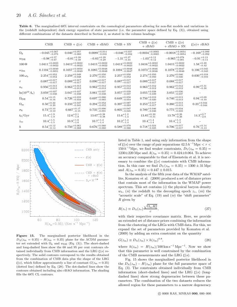
20 A.G. Sanchez et al.
Table 6. The marginalized 68% interval constraints on the cosmological parameters allowing for non-flat models and variations inthe (redshift independent) dark energy equation of state parameter (i.e. the parameter space defined by Eq. (3)), obtained usingdifferent combinations of the datasets described in Section 2, as stated in the column headings.
CMB CMB + ξ(s) CMB + rBAO CMB + SNCMB + ξ(s) CMB + ξ(s)
ξ(s)+ rBAO+ rBAO + rBAO + SN
Ωk −0.045+0.067−0.073 0.040+0.057
−0.060 0.0089+0.014−0.016 −0.046+0.037
−0.032 −0.0034+0.0065−0.0065 −0.0018+0.0054
−0.0054 −0.169+0.099−0.092
wDE −0.98+0.57−0.67 −0.81+0.39
−0.48 −0.83+0.29−0.29 −1.31+0.37
−0.34 −1.03+0.12−0.12 −0.965+0.078
−0.081 −0.91+0.13−0.14
100Θ 1.0411+0.0023−0.0022 1.0412+0.0022
−0.0022 1.0415+0.0022−0.0022 1.0413+0.0022
−0.0023 1.0416+0.0022−0.0022 1.0415+0.0022
−0.0022 1.58+0.39−0.42
ωdm 0.1104+0.0049−0.0051 0.1057+0.0050
−0.0049 0.1085+0.0048−0.0048 0.1094+0.0048
−0.0047 0.1073+0.0046−0.0046 0.1078+0.0047
−0.0046 0.106+0.045−0.043
100 ωb 2.254+0.052−0.054 2.259+0.049
−0.048 2.270+0.050−0.051 2.257+0.050
−0.052 2.274+0.050−0.050 2.270+0.046
−0.046 0.030+0.018−0.016
τ 0.087+0.017−0.017 0.089+0.017
−0.017 0.090+0.017−0.017 0.087+0.017
−0.017 0.089+0.017−0.017 0.088+0.017
−0.017 -
ns 0.956+0.013−0.013 0.963+0.013
−0.013 0.962+0.012−0.012 0.957+0.012
−0.012 0.963+0.012−0.012 0.962+0.012
−0.012 0.99+0.31−0.30
ln(1010As) 3.059+0.037−0.038 3.047+0.037
−0.038 3.061+0.037−0.038 3.057+0.039
−0.037 3.055+0.038−0.039 3.055+0.036
−0.037 -
ΩDE 0.54+0.15−0.16 0.726+0.033
−0.034 0.697+0.066−0.065 0.649+0.058
−0.054 0.750+0.019−0.020 0.740+0.013
−0.013 0.94+0.09−0.10
Ωm 0.50+0.22−0.20 0.233+0.047
−0.041 0.294+0.052−0.052 0.397+0.087
−0.093 0.253+0.017−0.017 0.260+0.013
−0.013 0.23+0.044−0.044
σ8 0.73+0.10−0.10 0.667+0.17
−0.15 0.735+0.090−0.091 0.805+0.047
−0.045 0.789+0.046−0.046 0.775+0.034
−0.033 -
t0/Gyr 15.4+1.9−1.9 12.6+2.1
−1.8 13.67+0.38−0.38 15.6+1.2
−1.4 13.85+0.30−0.31 13.78+0.26
−0.26 14.3+2.7−2.6
zre 10.4+1.5−1.5 10.9+1.6
−1.6 10.7+1.4−1.4 10.2+1.4
−1.4 10.4+1.4−1.4 10.4+1.3
−1.3 -
h 0.54+0.12−0.14 0.750+0.061
−0.068 0.676+0.060−0.060 0.589+0.070
−0.066 0.718+0.024−0.025 0.706+0.017
−0.017 0.76+0.14−0.13
Figure 15. The marginalized posterior likelihood in theDA(zm = 0.35) − H(zm = 0.35) plane for the ΛCDM parame-ter set extended with Ωk and wDE (Eq. (3)). The short-dashedand long-dashed lines show the 68 and 95 per cent contours ob-tained individually from CMB information and the LRG ξ(s) re-spectively. The solid contours correspond to the results obtainedfrom the combination of CMB data plus the shape of the LRGξ(s), which follow approximately a line of constant G(zm = 0.35)
(dotted line) defined by Eq. (28). The dot-dashed lines show thecontours obtained including also rBAO information. The shadingfills the 68% CL contours.
listed in Table 1, and using only information from the shapeof ξ(s) over the range of pair separations 42.5 h−1Mpc < r <150 h−1Mpc, we find weaker constraints, DV(zm = 0.35) =1230±220 Mpc and A(zm = 0.35) = 0.424±0.064. To achievean accuracy comparable to that of Eisenstein et al. it is nec-essary to combine the ξ(s) constraints with CMB informa-tion. In this case we find DV(zm = 0.35) = 1300 ± 31 Mpcand A(zm = 0.35) = 0.447 ± 0.015.
In the analysis of the fifth year data of the WMAP satel-lite, Komatsu et al. (2009) produced a set of distance priorsthat contain most of the information in the WMAP powerspectrum. This set contains (i) the physical baryon densitywb, (ii) the redshift to the decoupling epoch z∗, (iii) the“acoustic scale” of Eq. (19) and (iv) the “shift parameter”R given by
R(z∗) ≡ DA(z∗)
p
ΩmH20
c, (27)
with their respective covariance matrix. Here, we providean extended set of distance priors combining the informationfrom the clustering of the LRGs with CMB data. For this, weexpand the set of parameters provided by Komatsu et al.(2009) by adding an extra constraint on the quantity
G(zm) ≡ DA(zm) × h(zm)0.8, (28)
where h(zm) = H(zm)/100 kms−1 Mpc−1. Now we showthat this parameter is well constrained by the combinationof the CMB measurements and the LRG ξ(s).
Fig. 15 shows the marginalized posterior likelihood inthe DA(zm) − H(zm) plane for the full parameter space ofEq. (3). The constraints obtained individually from CMBinformation (short-dashed lines) and the LRG ξ(s) (long-dashed lines) show strong degeneracies between these pa-rameters. The combination of the two datasets reduces theallowed region for these parameters to a narrow degeneracy
c© 0000 RAS, MNRAS 000, 000–000

Cosmological parameters from the SDSS-DR6 LRGs ξ(s) 21
Figure 16. The marginalized posterior likelihood in the wDE −
Ωm plane for the ΛCDM parameter set extended with wDE
(Eq. (7)). The dashed lines show the 68 and 95 per cent contoursobtained using the full combination of CMB data plus the shapeof the LRG ξ(s). The solid contours correspond to the results ob-tained using the set of extended distance priors of Tables B1 andB2 of Appendix B. The shading fills the 68% CL contours.
(solid lines) which follows approximately a line of constantG (shown by the dotted line). For this combination we findthe constraint G(zm = 0.35) = 1175+18
−17 Mpc (a 1.4% error)which we include in our set of extended distance priors. Thedegeneracy between DA and H can be broken by includingan extra piece of information. In this case it is possible toobtain separate constraints on these parameters. Includingthe rBAO measurements (as shown by the dot-dashed linesin Fig. 15) we obtain DA(zm = 0.35) = 1363 ± 34 Mpc andH(zm = 0.35) = 83.3 ± 2.2 kms−1 Mpc−1. By using the SNdata instead we obtain DA(zm = 0.35) = 1336+80
−84 Mpc andH(zm = 0.35) = 86.4 ± 5.6 km s−1 Mpc−1.
The mean values and covariance matrix of the set ofextended distance priors obtained from the combination ofCMB information and the shape of the LRG ξ(s) are listedin Tables B1 and B2 of Appendix B. Fig. 16 shows a compar-ison of the marginalized constraints in the plane Ωm − wDE
for the parameter space of Eq. (7) obtained by using theset of extended distance priors (solid lines) and the ones ob-tained using the full CMB and ξ(s) data (dashed lines). Thisshows that this set of constraints contains the most relevantinformation from the combination of these datasets and canbe used to replace them to obtain constraints on cosmo-logical parameters in combination with other cosmologicalobservations like SN data or weak lensing, simplifying andaccelerating the required numerical procedure.
7 CONCLUSIONS
In this paper, we have applied a new model for the shapeof the correlation function at large pair separations to
the measurement of LRG clustering from the SDSS madeby Cabre & Gaztanaga (2009a). Using a full Monte-Carlomarkov chain analysis and combining the LRG measure-ments with the latest compilations of CMB and SNe data,we have presented a comprehensive set of constraints on cos-mological parameters for different combinations of datasetsand for different parameter spaces.
Large scale structure measurements and modelling havenow reached a level of precision where they provide con-straints on cosmological parameters which are competitivewith those obtained from other datasets. Using only theLRG correlation function and the measurement of the radialBAO peak, it is possible to determine the dark energy equa-tion of state parameter to wDE = −1.05+0.16
−0.15 . This providesfurther confirmation of the dark energy scenario, indepen-dent of CMB or SN observations.
The availability of several high quality datasets givesus the opportunity to scrutinize the derived constraints andto isolate possible systematic effects in either the observa-tions themselves or the theoretical model used to describethem. In general, different datasets are sensitive to differentparameter combinations and the constraints are optimizedwhen datasets are combined. However, in the case in whichdatasets are responsive to similar parameter combinations,it is important to check that consistent results are obtainedbefore combining the datasets. It would be meaningless tocombine two such datasets if a tension existed between theparameters values returned from each one individually.
The tables of parameter constraints given in this pa-per show that, to first order at least, the “Union” super-nova dataset of Kowalski et al. (2008) and the LRG clus-tering from the SDSS yield very similar constraints on cos-mological parameters when analysed in combination withCMB data, for all of the parameter spaces considered. Asshown in Section 5.2, the recovered value of the dark en-ergy equation of state in the CMB plus ξ(s) case of wDE =−0.996±0.090 shows a remarkable agreement with that ob-tained from the combination of CMB with the SN data ofwDE = −0.950 ± 0.055. The consistency of the constraintswe obtain from different combinations of datasets is a reas-suring validation of our analysis technique.
Percival et al. (2007c), however, found a tension at the2.4σ level between the constraints on DV(z = 0.35)/DV(z =0.20) coming from the BAO signal measured from galaxysamples drawn from the 2dFGRS and the SDSS (includ-ing a smaller LRG sample than the one considered here),and the SN data from Astier et al. (2006). When foldedwith the CMB data, this discrepancy leads to different pre-ferred values for the dark energy equation of state, with theSN data preferring wDE ≃ −1 and the BAO data point-ing to wDE < −1 with a significance of 1.4σ (see their fig-ures 12 and 13; see also Lazkoz et al. (2008)). Our analy-sis shows that the LRG clustering and SNe data give con-sistent constraints on the distance scale DV(z = 0.35).The tension reported by Percival et al. (2007c) could resultfrom the BAO signal at z = 0.2 (which corresponds to themain 2dFGRS and SDSS galaxy samples). This is unlikelyto be the answer, however, since the rBAO measurementsfrom Gaztanaga et al. (2008b), which separate the signalat z = 0.24 and z = 0.43, also give a consistent answer withwDE = −0.92 ± 0.15. The treatment of the BAO feature isquite different in the two analyses. Percival et al. (2007c)
c© 0000 RAS, MNRAS 000, 000–000

22 A.G. Sanchez et al.
effectively take a BAO template generated for a given setof cosmological parameters and then fit this to the mea-sured BAO features for different parameters. Furthermore,the technique of Percival et al. requires a reference spectrumto be defined. Finally, as Percival et al. (2007c) speculatethemselves, the problem could lie in the way in which theBAO are damped; these authors assume a fixed dampingscale, whereas we treat the damping scale as a parameter.
One criticism that could be levelled at our analysisis the apparent level of agreement between our new theo-retical model and the measured LRG clustering. We haveshown that the model is remarkably accurate when com-pared to the correlation function measured for the darkmatter or for samples of haloes drawn from N-body simula-tions (see also Crocce & Scoccimarro 2008; Sanchez et al.2008). However, in the case of the observed LRG clus-tering, the relative height of the BAO feature is greaterthan predicted by the model. This is illustrated in Fig. 17.This behaviour is not peculiar to the measurement byCabre & Gaztanaga (2009a). The earlier measurement ofLRG clustering by Eisenstein et al. (2005) had a similarform (see also Okumura et al. 2008). A key result from thispaper is the dependence of the parameter constraints on theminimum pair separation used in the analysis (Fig. 5). Themean parameter value returned is insensitive to the choice ofthe minimum pair separation; the only noticeable differenceis an increase in the 1σ range on selected parameters as fewerdata points are included. Similar conclusions were reachedusing a less challenging range of scales by Okumura et al.(2008). This confirms that the information we extract fromthe overall shape of the correlation function is consistentwith that contained in the BAO feature.
Fig. 17 also considers an extension to our best fittingmodel which involves allowing for a constant shift in ampli-tude (Sec 2.1.1). We have tested that the marginalizationover a constant additive term has a negligible impact on thecosmological constraints that we derive, which are driven byrelative changes in the goodness of fit. However, the addi-tion of this extra nuisance parameter can improve the ap-pearance of the fit and therefore reduce the absolute value ofχ2. If we use an absolute χ2 fit with the full covariance ma-trix, we find a probability of about 25% that our best fittingmodel describes the measured correlation function (the ex-act value varies between 20% and 33% depending on whichparameters we consider as degrees of freedom). If we allowfor a constant systematic shift, as argued in section 2.1.1, thebest fit model for the cosmological parameters remains thesame, but the probability of the model describing the dataimproves slightly to 60% in the range K = 0.003 − 0.006.This improvement is not significant enough to justify theextra parameter, despite the visual impact of this shift inFig. 17.
We used the combined information of the CMB mea-surements and the shape of the LRG ξ(s) to obtain a set ofdistance priors that combine the most relevant informationfrom these data sets to place constraints on dark energymodels and spatial curvature. For this, we expanded theset of distance priors provided by Komatsu et al. (2009)by adding a constraint on the quantity G(zm), defined inEq. (28), which is well constrained by the combination ofthese datasets (with an error of less than 2%). The meanvalues and covariance matrix of this extended set of dis-
Figure 17. Circles with error bars show the redshift space cor-relation function used in this paper (from Cabre & Gaztanaga2009a). The solid line corresponds to our best-fit model withinthe framework of the basic ΛCDM parameter space described inSec. 5.1, while the dashed line includes in addition a systematicK-shift with K = 0.0045. This shift may originate from unknownsystematic effects as described in Sec. 2.1.1. Even though the vi-sual impact seems important, this constant shift (note the biasfactor also changes) does not compromise the goodness of fit ofour best fitting model or the range of cosmological parametersderived in this paper. Our best fitting model (ie using K = 0)has a probability of 24 % to be in agreement with the data, ascompared with 62 % for the model with K = 0.0045. Thus thereis not a significant improvement on adding a constant shift to themodel.
tance priors are listed in Tables B1 and B2 of AppendixB. These can be used instead of the combination of CMBand ξ(s) data used in our analysis to obtain constraints oncosmological parameters in combination with other cosmo-logical observations, making the required calculations fasterand simpler.
Our analysis shows that current large-scale structuredatasets (using the shape of the correlation function atlarge pair separations, along with the form of the BAOpeak) give constraints on the basic cosmological parame-ters that are competitive with those from the best availableSNe datasets. Moreover, possible systematic distortions inthe clustering signal have been modelled extensively. Thetheoretical model applied in this paper has been shown toprovide an accurate description of the clustering for the levelof error expected in volumes up to two orders of magnitudelarger than the current LRG datasets. This bodes well forexperiments planned for ten year’s time, which will producesurveys covering volumes in the region of 100h−3Gpc3 (e.g.Cimatti et al. 2008). Nevertheless, it will be prudent to pur-sue as many approaches as possible to measure dark energyto allow comparisons to be made between the results ob-tained with different datasets, as carried out in this paper.
c© 0000 RAS, MNRAS 000, 000–000

Cosmological parameters from the SDSS-DR6 LRGs ξ(s) 23
ACKNOWLEDGEMENTS
We thank Francesco Montesano and Emilio Donoso fortheir assistance in preparing preliminary versions of manyof our plots. We thank Eiichiro Komatsu, Andres Bala-guera, Emiliano Sefusatti and Pablo Fosalba for useful com-ments and suggestions, and Roman Scoccimarro for pro-viding the simulation data. MC, AC and EG acknowl-edge support from Spanish Ministerio de Ciencia y Tec-nologia (MEC), project AYA2006-06341, Consolider-IngenioCSD2007-00060, research project 2005SGR00728 from Gen-eralitat de Catalunya and the Juan de la Cierva MEC pro-gram. We acknowledge the use of the Legacy Archive forMicrowave Background Data Analysis (LAMBDA). Supportfor LAMBDA is provided by the NASA Office of Space Sci-ence. This work was supported in part by the STFC.
REFERENCES
Ade P., ock J., Bowden M., Brown M. L., Cahill G., Carl-strom J. E., Castro P. G., Church, S., 2008, ApJ, 674,22
Albrecht, A., et al., 2006, preprint astro-ph/0609591Angulo R. E., Baugh C. M., Frenk C. S., Bower R.G., Jenk-ins A., Morris S. L., 2005, MNRAS, 362, L25
Angulo R. E., Baugh C. M., Frenk C. S., Lacey C. G., 2008,MNRAS, 383, 755
Astier P. et al., 2006, A&A, 447, 31Barris B. J. et al., 2004, ApJ, 602, 571Bennett C. L. et al., 2003, ApJS, 148, 1Blake C., Glazebrook K., 2003, ApJ, 594, 665Blanton M. R. et al., 2005, AJ, 129, 2562Bond J. R., Efstathiou G., Tegmark M., 1997, MNRAS,291, L33
Bridle S. L., Lahav O., Ostriker J. P., Steinhardt P. J.,2003, Science, 299, 1532
Cabre A., Gaztanaga E., 2009a, MNRAS, 393, 1183, eprintarXiv:0807.2460
Cabre A., Gaztanaga E., 2009b, MNRAS, 396, 1119, eprintarXiv:0807.2461
Chevallier M., Polarski D., 2001, Int. J. Mod. Phys. D., 10,213
Cimatti A. et al., 2008, Experimental Astronomy, in press,eprint arXiv:0804.4433
Cole S. et al. (The 2dFGRS Team), 2005, MNRAS, 362,505
Colless M. et al. (The 2dFGRS Team), 2001, MNRAS, 328,1039
Colless M. et al. (The 2dFGRS Team), 2003, eprintarXiv:0306581
Cresswell J.G., Percival W.J., 2009, MNRAS, 392, 682Crocce M., Scoccimarro R., 2006a, PRD, 73, 063519Crocce M., Scoccimarro R., 2006b, PRD, 73, 063520Crocce M., Scoccimarro R., 2008, PRD, 77, 023533Crocce M., Fosalba P., Castander F, Gaztanaga E., 2009,eprint arXiv:0907.0019
Desjacques V., 2008, PRD, 78, 103503Dunkley J. et al., 2009, ApJS, 180, 306Efstathiou G., Bond J. R., 1999, MNRAS, 304, 75Efstathiou G. et al., 2002, MNRAS, 330, L29Eisenstein D. J., Hu W., 1998, ApJ. 496, 605
Eisenstein D. J., Hu W., 1998, ApJ. 511, 5Eisenstein D. J. et al., 2001, AJ, 122, 2267Eisenstein D. J. et al., 2005, ApJ, 633, 560Eisenstein D. J., Seo H., Sirko E., Spergel D. N., 2006, ApJ,664, 675
Ellis R. S. et al., 2008, ApJ, 674, 51Estrada J., Sefusatti E., Frieman J. A., 2009, ApJ, 692, 265Fang W., Hu W., Lewis A., 2008, PRD, 78, 087303Ferramacho L. D., Blanchard A., Zolnierowski Y., 2009,A&A, 499, 21
Fosalba P., Gaztanaga, E., Castander F. J., Manera M.,2008, MNRAS, 391, 435
Gallagher J. S., Garnavich P. M., Berlind P., Challis P.,Jha S., Kirshner R. P., 2005, ApJ, 634, 210
Gaztanaga E., Cabre A., Castander F., Crocce M., FosalbaP., 2008a, MNRAS in press, eprint arXiv:0807.2448
Gaztanaga E., Cabre A., Hui L., 2008b, MNRAS in press,eprint arXiv:0807.3551
Gaztanaga E., Miquel R., Sanchez E., 2008c, eprintarXiv:0808.1921
Gelman A., Rubin D., 1992, Stat. Sci., 7, 457Gorski K. M., Wandelt B. D., Hansen F. K., Hivon E.,Banday A. J., 1999, eprint arXiv:9905275
Glazebrook K. et al. 2007, ASPC, 379, 72Guzik J., Bernstein G., Smith R. E., 2007, MNRAS, 375,1329
Guy J., Astier P., Nobili S., Regnault N., Pain R., 2005,A&A, 443, 781
Hamann J., Hannestad S., Melchiorri A., Wong Y. Y. Y.,2008, JCAP, 07, 017
Hicken M., Wood-Vasey W.M., Blondin S., Challis P.,Jha S., Kelly P.L., Rest A., Kirshner R.P., 2009, eprintarXiv:0901.4804
Hinshaw G. et al., 2003, ApJS, 148, 135Hinshaw G. et al., 2007, ApJS, 170, 288Hinshaw G. et al., 2009, ApJS, 180, 225Hogg D.W., Eisenstein D.J., Blanton M.R., Bahcall N.A.,Brinkmann J., Gunn J.E., Schneider D.P., 2005, ApJ, 624,54
Howell D. A. et al., 2009, ApJ, 691, 661Hu W., Haiman Z., 2003, PRD, 68, 063004Hu W., Jain B., 2004, PRD, 70, 043009Huff E., Schulz A. E., White M., Schlegel D. J., WarrenM. S., 2007, Astroparticle Physics, 26, 351
Huterer D., Turner M.S., 2001, PRD, 64, 123527Hutsi G., 2006, A&A, 449, 891Hutsi G., 2007, MNRAS, submitted, eprintarXiv:0705.1843
Jones W. C. et al., 2006, ApJ, 647, 823Kaiser N., 1987, MNRAS, 227, 1Komatsu E. et al., 2009, ApJS, 180, 330Kowalski M. et al., 2008, ApJ, 686, 749Kuo C. L. et al., 2007, ApJ, 664, 687Lazkoz R., Nesseris S., Perivolaropoulos L., 2008, JCAP,07, 012
Lee A. T. et al., 2001, ApJ, 561, L1Lewis A., Bridle, S., 2002, PRD, 66, 103511Lewis A., Challinor A., Lasenby A., 2000, ApJ, 538, 473Linder E. V., 2003, PRL, 90, 091301Martinez V. J., Arnalte-Mur P., Saar E., de la Cruz P.,Pons-Borderia M. J., Paredes S., Fernandez-Soto A., Tem-pel E., 2009, ApJ, 696L, 93
c© 0000 RAS, MNRAS 000, 000–000

24 A.G. Sanchez et al.
Matarrese S., Pietroni M., 2007, JCAP, 06, 026Matsubara T., 2004, ApJ, 615, 573Matsubara T., 2008, PRD, 77, 063530Meiksin A., White M., Peacock J. A., 1999, MNRAS, 304,851
Miknaitis G. et al., 2007, ApJ, 666, 674Montroy T. E. et al., 2006, ApJ, 647, 813Nolta M. R. et al., 2009, ApJS, 180, 296Norberg P., Baugh C. M., Gaztanaga E., Croton D. J.,2009, MNRAS, 396, 19
Okumura T., Matsubara T., Eisenstein D. J., Kayo I., Hik-age C., Szalay A. S., Schneider D. P., 2008, ApJ, 676, 889
Padmanabhan N., et al., 2007, MNRAS, 378, 852Page L. et al., 2003, ApJS, 148, 233Percival W. J. et al., 2002, MNRAS, 337, 1068Percival W. J. et al., 2007a, ApJ, 657, 51Percival W. J. et al., 2007b, ApJ, 657, 645Percival W.J., Cole S., Eisenstein D. J., Nichol R. C., Pea-cock J. A., Pope A. C., Szalay A. S., 2007, MNRAS, 381,1053
Percival W. J., White M., 2009, MNRAS, 393, 297Perlmutter S. et al., 1999, ApJ, 517, 565Piacentini F. et al., 2006, ApJ, 647, 833Pietroni M., 2008, JCAP, 10, 036Readhead A. C. et al., 2004, ApJ, 609, 498Reichardt C. L. et al., 2009, ApJ, 694, 1200Reid B. A., Spergel D. N., Bode P., 2008, ApJ, submitted,eprint arXiv:0811.1025
Riess A. G. et al., 1998, AJ, 116, 1009Riess A. G. et al., 2004, ApJ, 607, 665Riess A. G. et al., 2007, ApJ, 659, 98Ruhl J. E. et al., 2003, ApJ, 599, 786Sanchez A. G., Baugh C. M., Percival W. J., Peacock J. A.,Padilla N. D., Cole S., Frenk C. S., Norberg P., 2006,MNRAS, 366, 189
Sanchez A.G., Cole S., 2008, MNRAS, 385, 830Sanchez A.G., Baugh C.M., Angulo R., 2008, MNRAS, 390,1470
Scoccimarro R., 2004, PRD, 70, 083007Seljak U. et al., 2005, PRD, 71, 103515Seljak U., Slosar A., McDonald P., 2006, JCAP, 10, 014Seo H., Eisenstein D. J., 2003, ApJ, 598, 720Seo H., Eisenstein D. J., 2007, ApJ, 665, 14Seo H., Siegel E. R., Eisenstein D. J., White M., 2008, ApJ,686, 13
Smith R. E., Peacock J. A., Jenkins A., White, S. D. M.,Frenk C. S., Pearce F. R., Thomas P. A., Efstathiou G.,Couchman H. M. P., 2008, MNRAS, 341, 1311
Smith R. E., Scoccimarro R., Sheth R. K., 2007, PRD, 75,063512
Smith R. E., Scoccimarro R., Sheth R. K., 2008, PRD, 77,043525
Spergel D. N. et al., 2003, ApJS, 148, 175Spergel D. N. et al., 2007, ApJS, 170, 377Steigman G., 2007, on SUSY06: The 14th InternationalConference on Supersymmetry and the Unification of Fun-damental Interactions Edited by Feng J.L., p.40
Sugiyama N., 1995, ApJS, 100, 281Sullivan M. et al., 2003, MNRAS, 340, 1057Swanson M.E.C., Tegmark M., Blanton M., Zehavi I., 2008,MNRAS, 385, 1635
Szapudi I., 2004, ApJ, 614, 51
Takahashi R. et al., 2008, MNRAS, 389, 1675Taruya A., Hiramatsu T., 2008, ApJ, 674, 617Tegmark M., Silk, J., Blanchard A., 1994, ApJ, 420, 484Tegmark M. et al., 2004, ApJ 606, 702Tegmark M. et al, 2006, PRD, 74, 123507Tonry J. L. et al., 2003, ApJ, 594, 1Wood-Vasey W. M.et al., 2007, ApJ, 666, 694Wang Y., 2006, ApJ, 647, 1Wang Y., Mukherjee P., 2006, ApJ, 650, 1Wood-Vasey M., et al. 2007, ApJ, 666, 694Wright E.L., 2007, ApJ, 664, 633Xia J., Li H., Zhao G., Zhang X., 2008, PRD, 78, 0835524
APPENDIX A: THE THEORETICAL
MOTIVATION FOR THE MODEL FOR THE
SHAPE OF ξ(R)
In recent years substantial progress has been made inunderstanding the non-linear gravitational evolution ofdensity fluctuations (Crocce & Scoccimarro 2006a, 2008;Matarrese & Pietroni 2007; Matsubara 2008; Pietroni2008; Taruya & Hiramatsu 2008). Within the theoreticalframework of Renormalized Perturbation Theory (RPT),Crocce & Scoccimarro (2006a,b) showed that the evolutionof the power spectrum from its initial value in the linearregime, PL(k), can be described as the sum of two contribu-tions
PNL(k, z) = PL(k)G2(k, z) + PMC(k, z), (A1)
where G is the nonlinear propagator which weights howmuch power can be directly linked to the linear epoch (e.g.damping the higher BAO harmonics), and PMC representsthe new variance generated by mode coupling.
In configuration space, the first term in Eq. (A1) leadsto a convolution of the linear theory correlation func-
tion with a nearly Gaussian kernel (since G ∼ e−k2
, seeCrocce & Scoccimarro (2006b)), which causes the acousticpeak to broaden and shift to smaller values (Smith et al.2008; Crocce & Scoccimarro 2008). In turn, the contri-bution of the mode-coupling term can be computed toleading order at large pair separation, yielding ξMC(r) ∝ξ′L(r) ξ
(1)L (r) (Crocce & Scoccimarro 2008), where ξ′L(r) is
the first derivative of the linear theory correlation functionand ξ
(1)L (r) is defined by Eq (11).
In fact, Eq.( A1) is also valid for the nonlinear spectraof density (δ)/velocity divergence (θ) fields, Pδθ and Pθθ,
PNL,ab = PLGaGb + PMC,ab, (A2)
with a = δ, θ.To study the impact of redshift distortions and bias we
put together the discussion above and the ansatz given inScoccimarro (2004) (see also Percival & White (2009)):
Ps(k) = e−k2f2µ2σ2
v
ˆ
b2Pδδ + 2fµ2bPδθ + f2µ4Pθθ
˜
, (A3)
where Pδδ, Pδθ and Pθθ were introduced above and a locallinear bias relation between the density fluctuations in thedistribution of galaxies and dark matter is assumed (butwith unbiased galaxy velocities). The damping factor inEq. (A3) arises after assuming a Gaussian PDF for the pair-wise velocities with rms (if evaluated in the linear regime),
c© 0000 RAS, MNRAS 000, 000–000

Cosmological parameters from the SDSS-DR6 LRGs ξ(s) 25
σv =1
3
Z
PL(q)
q2d3q. (A4)
In Eq. (A3) f is the logarithmic derivative of the lineargrowth rate with respect to the scale factor, f = d lnD/d lna,and µ = kz/k is the cosine of the line-of-sight angle. Notethat the small scale redshift space distortions, commonly re-ferred to as “fingers of God” (FOG) due to the elongation ofvirialised structures, are difficult to model accurately, partlydue to the non-Gaussianity of the PDF, which persists evento large scales (Scoccimarro 2004). In addition, the damp-ing factor depends on galaxy type (or mean halo mass andsatellite population)
We are interested in the monopole of the correlationfunction, i.e. the angle average of the Fourier transform ofPs(k) in Eq. (A3). Since the time required to evaluate thedifferent power spectra is not well suited to the explorationof large parameter spaces, we would like to motivate a para-metric description of the problem.
Crocce & Scoccimarro (2006b) showed that both Gθ
and Gδ are of approximately Gaussian form, and with sim-ilar smoothing length. Therefore the main contribution tothe correlation function at large separations can be mod-
eled, combining Eqs. (A3,A2), as ∝ ξL ⊗ e−(k⋆r)2 . The FOGprefactor in Eq.(A3) leads to an extra suppression, whichis subdominant to that of nonlinear gravity for low redshiftdata (where f ∼ 0.5). However, it can be accounted for tosome degree by smaller values of k⋆.
The mode coupling spectra in Eq. (A2) do differ at theseveral % level (Scoccimarro 2004), but they all give con-tributions scaling as ∼ ξ′ (the derivative of the correlationfunction) in configuration space at large separations. Theconvolution with the FOG suppression leaves this contribu-tion unaltered as the smoothing length introduced by theFOG is smaller than features present in ξ′, even at BAOscales.
Therefore we are left with the following parametriza-tion,
ξNL(r) = b2ξL(r) ⊗ e−(k⋆r)2 + AMC ξ′L(r) ξ(1)L (r), (A5)
for the correlation function at large pair separations in red-shift space, where b and AMC are nuisance parameters toaccount for bias and also the enhanced correlation ampli-tude due to redshift distortions (Kaiser 1987).
The assumptions behind the model in Eq. (A5), onecould argue, are over-simplifications, particularly for biasedtracers such as LRGs (Zehavi et al. 2005; Blake et al. 2007),or for deeper surveys where a more systematic derivation ofredshift distortions may be needed. Nonetheless this formis well motivated given the size of statistical errors in theSDSS-DR6 LRG sample, and based on results from Sec. 3.2(see also Sanchez et al. (2008)) should be accurate also forfuture larger surveys.
APPENDIX B: EXTENDED DISTANCE
PRIORS
Here we list the constraints on the set of extended distancepriors described in Section 6. Table B1 lists the mean val-ues and variances of the parameters in this set and Table B2gives the corresponding covariance matrix. This information
Table B1. The mean values and variances of the parametersin the set of extended distance priors described in Section 6, us-ing the compilation of CMB data in combination with the LRGcorrelation function.
Parameter value
100ωb 2.28 ± 0.55z∗ 1090.12 ± 0.93
ℓA(z∗) 301.58 ± 0.67R(z∗) 1.701 ± 0.018G(zm) 1175 ± 21
can be used to replace the CMB and ξ(s) data in multipara-metric analysis since it contains most of the information ofthe combination of these two datasets. With this simplifi-cation, the likelihood of a given cosmological model can beeasily computed as −2 lnL ∝ (D−T)t C
−1(D−T)t whereD is a vector containing the constraints of Table B1, T con-tains the corresponding prediction for a given cosmologicalmodel and C
−1 is the inverse of the covariance matrix of Ta-ble B2. This procedure considerably reduces the computingtime required to obtain constraints on cosmological param-eters compared with the full analysis of the data and can beused in combination with other datasets like weak lensingor the Hubble diagram of type Ia supernovae.
c© 0000 RAS, MNRAS 000, 000–000

26 A.G. Sanchez et al.
Table B2. The covariance matrix of the parameters in the set of extended distance priors described in Section 6.
100ωb z∗ ℓA(z∗) R(z∗) G(zm)100ωb 2.99 × 10⁻⁷ −4.2030 × 10⁻⁴ −1.9988 × 10⁻⁴ −3.4393 × 10⁻⁶ −1.9978 × 10−3
z∗ 8.6812 × 10−1 0.2557 1.1999 × 10⁻¹ 3.2355ℓA(z∗) 0.4558 3.1265 × 10⁻² 1.8247R(z∗) 3.1460 × 10⁻⁴ 3.9649 × 10⁻²
G(zm) 4.3784 × 10²
c© 0000 RAS, MNRAS 000, 000–000
Related Documents