10 Nov'08 Comp30291 DMP Section 5 1 University of Manchester School of Computer Science Comp 30291 : Digital Media Processing Section 5 z-transforms & IIR-type digital filters

10 Nov'08Comp30291 DMP Section 51 University of Manchester School of Computer Science Comp 30291 : Digital Media Processing Section 5 z-transforms & IIR-type.
Dec 14, 2015
Welcome message from author
This document is posted to help you gain knowledge. Please leave a comment to let me know what you think about it! Share it to your friends and learn new things together.
Transcript
10 Nov'08 Comp30291 DMP Section 5 1
University of ManchesterSchool of Computer Science
Comp 30291 : Digital Media Processing
Section 5
z-transforms & IIR-type digital filters
10 Nov'08 Comp30291 DMP Section 5 2
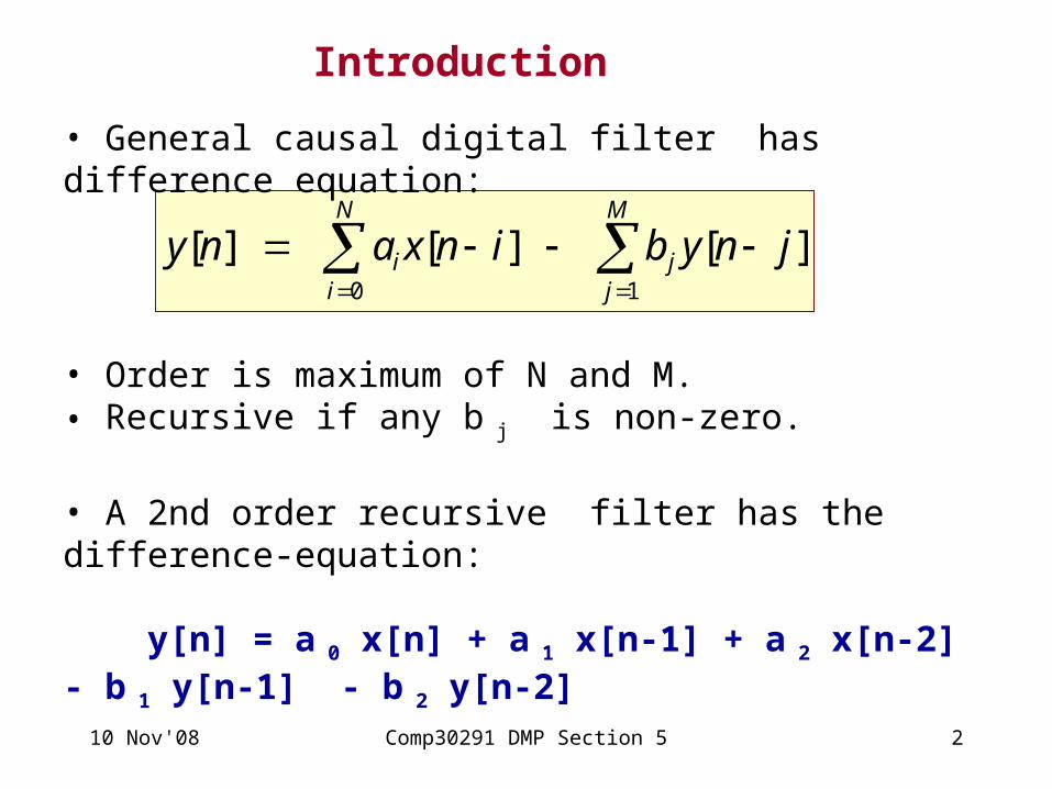
• Order is maximum of N and M. • Recursive if any b j is non-zero.
• A 2nd order recursive filter has the difference-equation:
y[n] = a 0 x[n] + a 1 x[n-1] + a 2 x[n-2] - b 1 y[n-1] - b 2 y[n-2]
N
i
M
jji jnybinxany
0 1
][ ][ ][
Introduction
• General causal digital filter has difference equation:
10 Nov'08 Comp30291 DMP Section 5 3
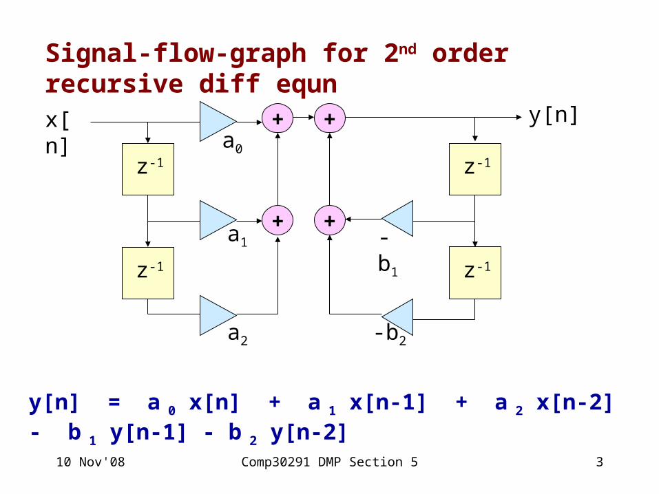
y[n] = a 0 x[n] + a 1 x[n-1] + a 2 x[n-2] - b 1 y[n-1] - b 2 y[n-2]
Signal-flow-graph for 2nd order recursive diff equn
z-1
z-1
z-1
z-1
+
+
+
+a0
a1
a2
x[n]
-b2
-b1
y[n]

10 Nov'08 Comp30291 DMP Section 5 4
Derivation of ‘z-transform’
transform)-(z ][ ][)( where
)(
][
][
][][
n
n
m
m
n
m
mn
m
mn
m
mn
znhzmhzH
zHz
zmhz
zzmh
zmhny
If {x[n]} with x[n] = zn is applied to an LTI system with impulse-response {h[n]}, output would be, by convolution :
10 Nov'08 Comp30291 DMP Section 5 5
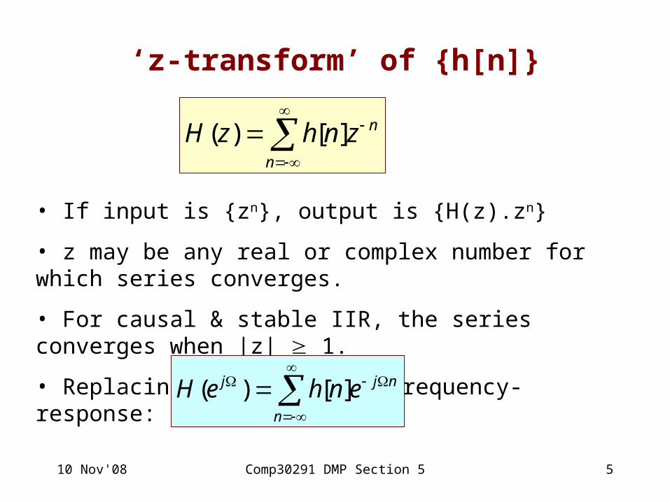
‘z-transform’ of {h[n]}
n
nznhzH ][)(
• If input is {zn}, output is {H(z).zn}
• z may be any real or complex number for which series converges.
• For causal & stable IIR, the series converges when |z| 1.
• Replacing z by ej gives frequency-response:
n
njj enheH ][)(

10 Nov'08 Comp30291 DMP Section 5 6
Visualising H(z) On Argand diagram (‘z-plane’), z = ej lies on unit circle.
Imaginary part of z
Real part of z1
z = ej

10 Nov'08 Comp30291 DMP Section 5 7
Example 5.1
Find H(z) for the non-recursive difference equation:
y[n] = x[n] + x[n-1]
Solution:
{h[n]} = { ... , 0, 1, 1, 0, ... },
therefore
H(z) = 1 + z - 1
10 Nov'08 Comp30291 DMP Section 5 8
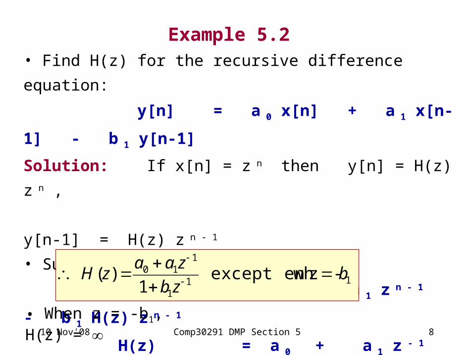
Example 5.2 • Find H(z) for the recursive difference equation:
y[n] = a 0 x[n] + a 1 x[n-1] - b 1 y[n-1]
Solution: If x[n] = z n then y[n] = H(z) z n ,
y[n-1] = H(z) z n - 1
• Substitute to obtain:
H(z) z n = a 0 z n + a 1 z n - 1 - b 1 H(z) z n - 1
H(z) = a 0 + a 1 z - 1 - b 1 H(z) z - 1
(1 + b1z-1) H(z) = a 0 + a 1 z - 1
-zen except wh 1
)( 111
110 bzb
zaazH
• When z = -b1, H(z) =
10 Nov'08 Comp30291 DMP Section 5 9
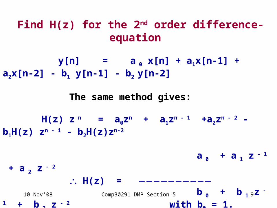
Find H(z) for the 2nd order difference-equation y[n] = a 0 x[n] + a1x[n-1] + a2x[n-2] - b1 y[n-1] - b2 y[n-2] The same method gives: H(z) z n = a0zn + a1zn - 1 +a2zn - 2 - b1H(z) zn - 1 - b2H(z)zn-2
a 0 + a 1 z - 1 + a 2 z - 2
H(z) = b 0 + b 1 z - 1 + b 2 z - 2 with b0 = 1.
10 Nov'08 Comp30291 DMP Section 5 10
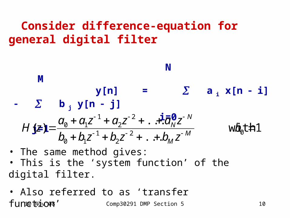
Consider difference-equation for general digital filter
N M y[n] = a i x[n i] b j y[n j] i=0 j=1
• The same method gives:
1 with ...
...)( 02
21
10
22
110
bzbzbzbb
zazazaazH
MM
NN
• This is the ‘system function’ of the digital filter.
• Also referred to as ‘transfer function’
10 Nov'08 Comp30291 DMP Section 5 11
• Ratio of 2 polynomials in z-1
• Equal to z-transform of impulse-response when this converges.
• Easily derived from difference-equation & signal-flow graph.
• Replacing z by ej gives frequency-response
System function

10 Nov'08 Comp30291 DMP Section 5 12
Example 5.3 Give a signal-flow graph for the system function:
22
11
22
110
1)(
zbzb
zazaazH
Solution: The difference-equation is: y[n] = a0 x[n] + a1 x[n-1] + a2 x[n-2] - b1 y[n-1] - b2 y[n-2]Represented by the signal-flow graph below:
2nd order or ‘bi-quadratic’ IIR section in ‘direct form 1’.
z-1
z-1
z-1
z-1
+
+
+
+a0
a1
a2
x[n]
-b2
-b1
y[n]
10 Nov'08 Comp30291 DMP Section 5 13
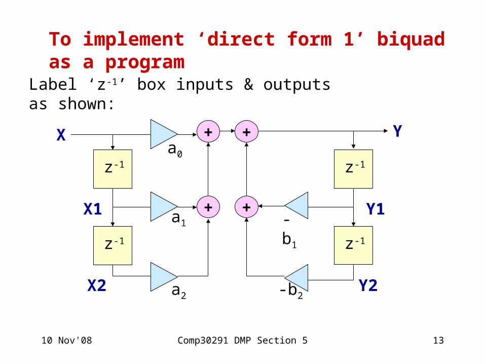
Label ‘z-1’ box inputs & outputs as shown:
To implement ‘direct form 1’ biquad as a program
z-1
z-1
z-1
z-1
+
+
+
+a0
a1
a2
X
-b2
-b1
Y
X1
X2
Y1
Y2
10 Nov'08 Comp30291 DMP Section 5 14
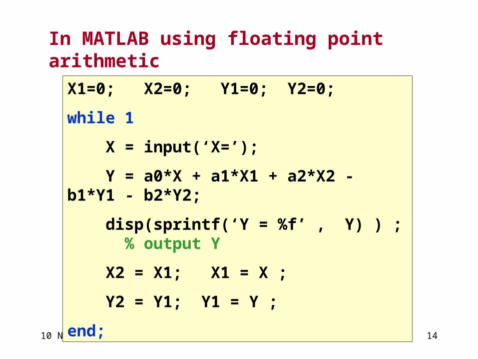
X1=0; X2=0; Y1=0; Y2=0;
while 1
X = input(‘X=’);
Y = a0*X + a1*X1 + a2*X2 - b1*Y1 - b2*Y2;
disp(sprintf(‘Y = %f’ , Y) ) ; % output Y
X2 = X1; X1 = X ;
Y2 = Y1; Y1 = Y ;
end;
In MATLAB using floating point arithmetic
10 Nov'08 Comp30291 DMP Section 5 15
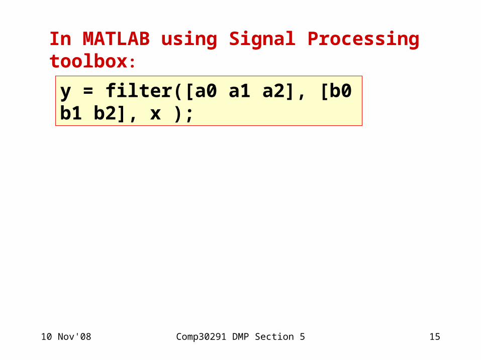
y = filter([a0 a1 a2], [b0 b1 b2], x );
In MATLAB using Signal Processing toolbox:
10 Nov'08 Comp30291 DMP Section 5 16
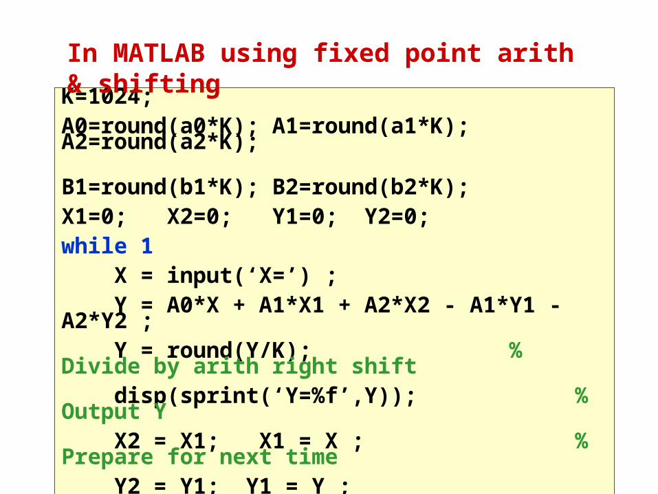
K=1024;A0=round(a0*K); A1=round(a1*K); A2=round(a2*K); B1=round(b1*K); B2=round(b2*K);X1=0; X2=0; Y1=0; Y2=0;while 1 X = input(‘X=’) ; Y = A0*X + A1*X1 + A2*X2 - A1*Y1 - A2*Y2 ; Y = round(Y/K); % Divide by arith right shift disp(sprint(‘Y=%f’,Y)); % Output Y X2 = X1; X1 = X ; % Prepare for next time Y2 = Y1; Y1 = Y ;end;
In MATLAB using fixed point arith & shifting
10 Nov'08 Comp30291 DMP Section 5 17
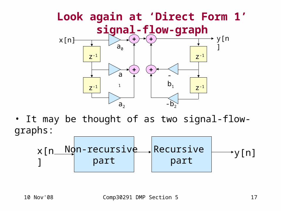
Look again at ‘Direct Form 1’ signal-flow-graph
• It may be thought of as two signal-flow-graphs:
z-1
z-1
z-1
z-1
+
+
+
+a0
a1
a2
x[n]
-b2
-b1
y[n]
Non-recursive part
Recursive part
x[n] y[n]
10 Nov'08 Comp30291 DMP Section 5 18
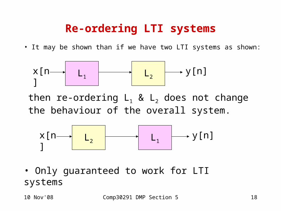
Re-ordering LTI systems
• It may be shown than if we have two LTI systems as shown:
L1 L2x[n] y[n]
L2 L1x[n] y[n]
then re-ordering L1 & L2 does not change the behaviour of the overall system.
• Only guaranteed to work for LTI systems
10 Nov'08 Comp30291 DMP Section 5 19
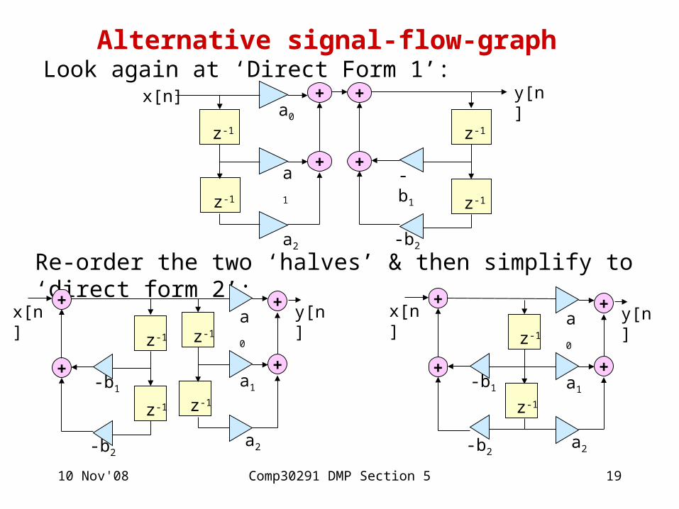
Alternative signal-flow-graph Look again at ‘Direct Form 1’:
Re-order the two ‘halves’ & then simplify to ‘direct form 2’:
x[n]
z-1
z-1
z-1
z-1
+
+
+
+a0
a1
a2 -b2
-b1
y[n]
a2
x[n]
z-1
z-1
+
+a0
a1
-b2
z-1
z-1
+
+
-b1
y[n]
a2
z-1
z-1
+
+a0
a1
y[n]x[n]
-b2
+
+
-b1

10 Nov'08 Comp30291 DMP Section 5 20
‘Direct Form II’ signal-flow-graph
Its difference equation is: y[n] = a 0 x[n] + a 1 x[n-1] + a 2 x[n-2] - b 1 y[n-1] - b 2 y[n-2]i.e. exactly the same as Direct Form 1
22
11
22
110
1)(
zbzb
zazaazH
It is a 2nd order (bi-quad) section whose system function is:a2
z-1
z-1
+
+a0
a1
y[n]x[n]
-b2
+
+
-b1
W
W1
W2
• Direct form II economises on ‘delay boxes’.
• Notice labels: W,W1 & W2

10 Nov'08 Comp30291 DMP Section 5 21
W1 = 0; W2 = 0; %For delay boxes while 1 X = input(‘X=’) ; % Input to X W =X - b1*W1 - b2*W2; % Recursive part Y = W*a0 + W1*a1 + W2*a2; % Non-rec. part W2 = W1; W1 = W; % For next time disp(sprintf(‘Y=%f’,Y)); % Output Y using disp end; % Back for next sample
Program to implement Direct Form II using normal arithmetic

10 Nov'08 Comp30291 DMP Section 5 22
K=1024;A0=round(a0*K); A1=round(a1*K); A2=round(a2*K); B1=round(b1*K); B2=round(b2*K);W1 = 0; W2 = 0; %For delay boxes while 1 X = input(‘X=’) ; % Assign X to input W =K*X - B1*W1 - B2*W2; % Recursive part W =round( W / K); % By arith right-shift Y = W*A0+W1*A1+W2*A2; % Non-rec. part W2 = W1; W1 = W; %For next time Y = round(Y/K); %By arith right-shift disp(sprintf( ‘Y=%f’, Y)); %Output Y using dispend; % Back for next sample
Direct Form II in fixed point arithmetic with shifting
10 Nov'08 Comp30291 DMP Section 5 23
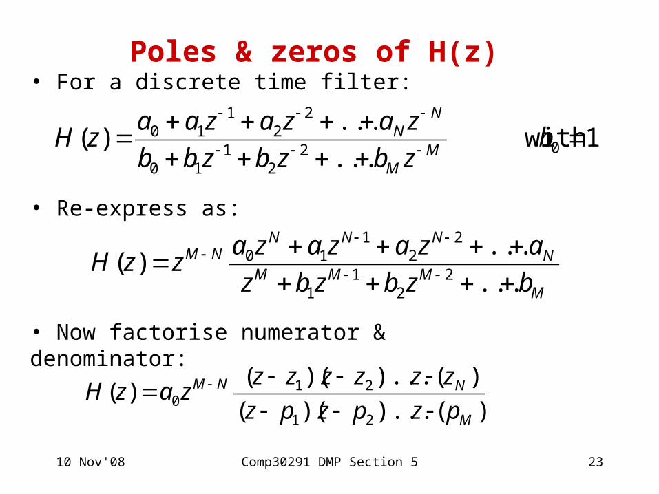
• Re-express as:
1 with ...
...)( 02
21
10
22
110
bzbzbzbb
zazazaazH
MM
NN
Poles & zeros of H(z)• For a discrete time filter:
MMMM
NNNN
NM
bzbzbz
azazazazzH
...
...)(
22
11
22
110
• Now factorise numerator & denominator:
))...()((
))...()(()(
21
210
M
NNM
pzpzpz
zzzzzzzazH
10 Nov'08 Comp30291 DMP Section 5 24
Poles & zeros of H(z) continued
• z 1 , z 2 ,..., z N , are ‘zeros’. p 1 ,p 2 ,..., p N , are ‘poles’.
• H(z) generally infinite with z equal to a pole.
• H(z) generally zero with z equal to a zero.
• For a causal stable system all poles must satisfy p i < 1.
i.e. on Argand diagram: poles must lie inside unit circle.
• No restriction on the positions of zeros.
10 Nov'08 Comp30291 DMP Section 5 25
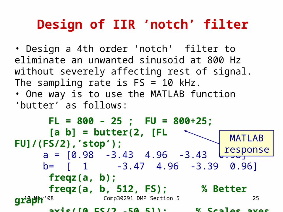
Design of IIR ‘notch’ filter
• Design a 4th order 'notch' filter to eliminate an unwanted sinusoid at 800 Hz without severely affecting rest of signal. The sampling rate is FS = 10 kHz.• One way is to use the MATLAB function ‘butter’ as follows:
FL = 800 – 25 ; FU = 800+25; [a b] = butter(2, [FL FU]/(FS/2),’stop’);
a = [0.98 -3.43 4.96 -3.43 0.98]b= [ 1 -3.47 4.96 -3.39 0.96]
freqz(a, b); freqz(a, b, 512, FS); % Better graph axis([0 FS/2 -50 5]); % Scales axes
• Notch has -3 dB frequency band: 25 + 25 = 50 Hz.
MATLAB response
10 Nov'08 Comp30291 DMP Section 5 26
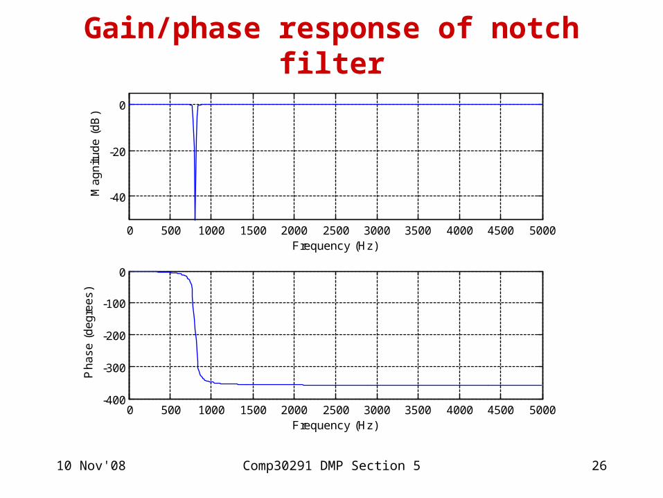
Gain/phase response of notch filter
0 500 1000 1500 2000 2500 3000 3500 4000 4500 5000-400
-300
-200
-100
0
Frequency (Hz)
Ph
as
e (
de
gre
es
)
0 500 1000 1500 2000 2500 3000 3500 4000 4500 5000
-40
-20
0
Frequency (Hz)
Ma
gn
itu
de
(d
B)
10 Nov'08 Comp30291 DMP Section 5 27
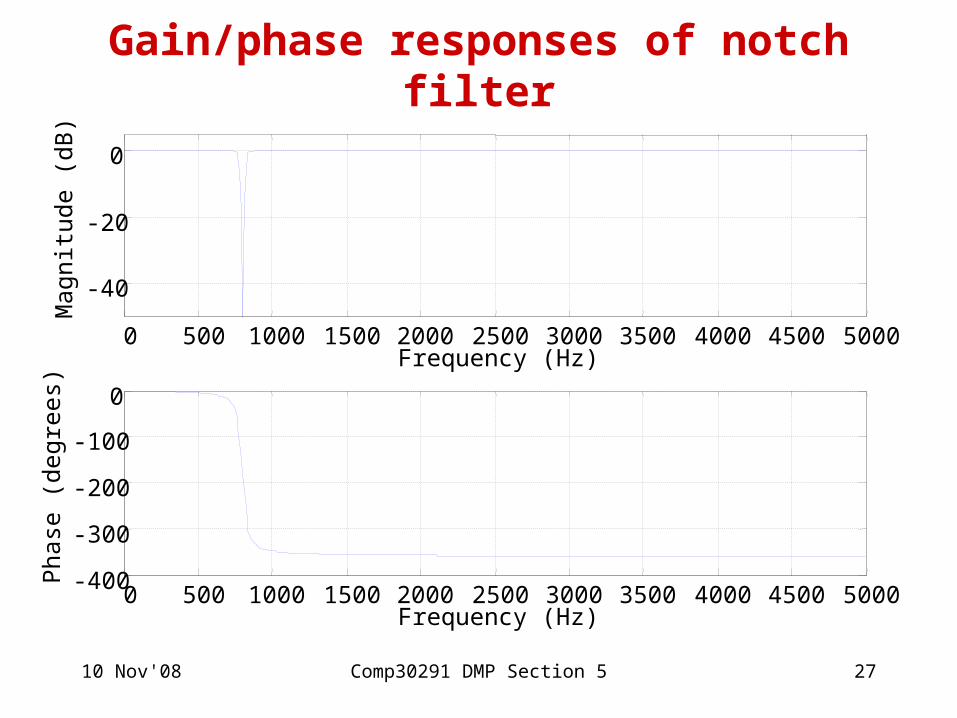
Gain/phase responses of notch filter
0 500 1000 1500 2000 2500 3000 3500 4000 4500 5000-400
-300
-200
-100
0
Frequency (Hz)
Pha
se (
degr
ees)
0 500 1000 1500 2000 2500 3000 3500 4000 4500 5000
-40
-20
0
Frequency (Hz)
Mag
nitu
de (
dB)
10 Nov'08 Comp30291 DMP Section 5 28
• How sharp is the notch? • Can answer this question by specifying notch’s -3 dB bandwidth.• Have just designed what Barry calls a 4th order band-stop filter.• MATLAB calls it a 2nd order band-stop filter. • For a sharper notch, decrease -3 dB bandwidth• But this will decrease its ‘depth’,
i.e. the attenuation at the ‘notch’ frequency.• If necessary, increase the order to 6 (3) or 8 (4).
Details
10 Nov'08 Comp30291 DMP Section 5 29
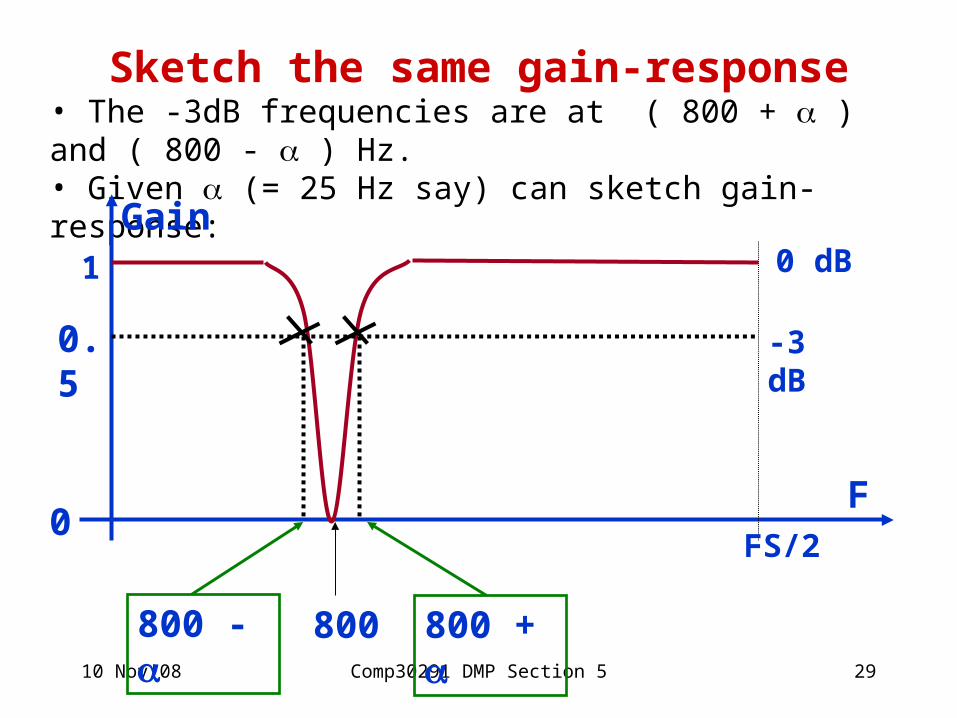
Sketch the same gain-response • The -3dB frequencies are at ( 800 + ) and ( 800 - ) Hz. • Given (= 25 Hz say) can sketch gain-response:
1
FS/2
F
Gain
0.5
0
800 800 + 800 -
0 dB
-3 dB

10 Nov'08 Comp30291 DMP Section 5 30
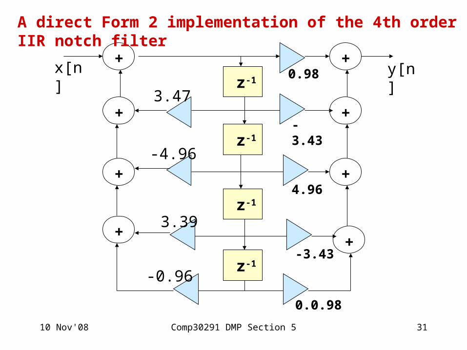
Implement the 4th order ‘notch’ filter
MATLAB function gave us:
a = [0.98 -3.43 4.96 -3.43 0.98]
b= [ 1 -3.47 4.96 -3.39 0.96]
Transfer (System) Function is:
4321
4321
96.039.396.447.31
98.043.396.443.398.0
zzzz
zzzzzH
10 Nov'08 Comp30291 DMP Section 5 31
z-1
z-1
z-1
z-1
+
+
+
+
+
+
+
+
0.98
3.47
-4.96
3.39
-0.96
0.0.98
x[n] y[n]
-3.43
4.96
-3.43
A direct Form 2 implementation of the 4th order IIR notch filter
10 Nov'08 Comp30291 DMP Section 5 32
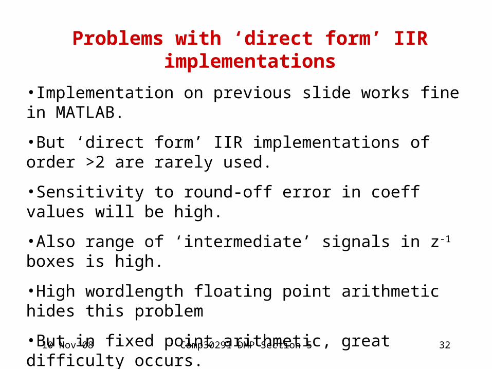
Problems with ‘direct form’ IIR implementations
•Implementation on previous slide works fine in MATLAB.
•But ‘direct form’ IIR implementations of order >2 are rarely used.
•Sensitivity to round-off error in coeff values will be high.
•Also range of ‘intermediate’ signals in z-1 boxes is high.
•High wordlength floating point arithmetic hides this problem
•But in fixed point arithmetic, great difficulty occurs.
•Instead we use ‘cascaded biquad sections’
10 Nov'08 Comp30291 DMP Section 5 33
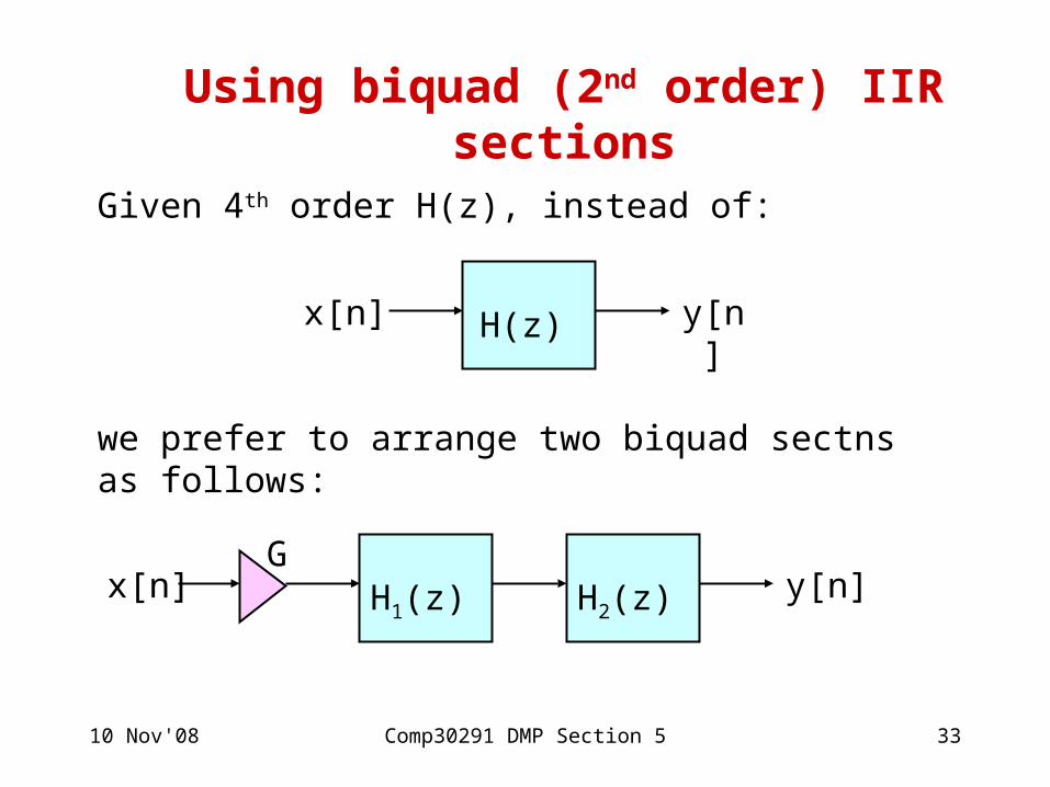
Using biquad (2nd order) IIR sections
H(z)x[n] y[n]
Given 4th order H(z), instead of:
we prefer to arrange two biquad sectns as follows:
H1(z) H2(z)x[n] y[n]G
10 Nov'08 Comp30291 DMP Section 5 34
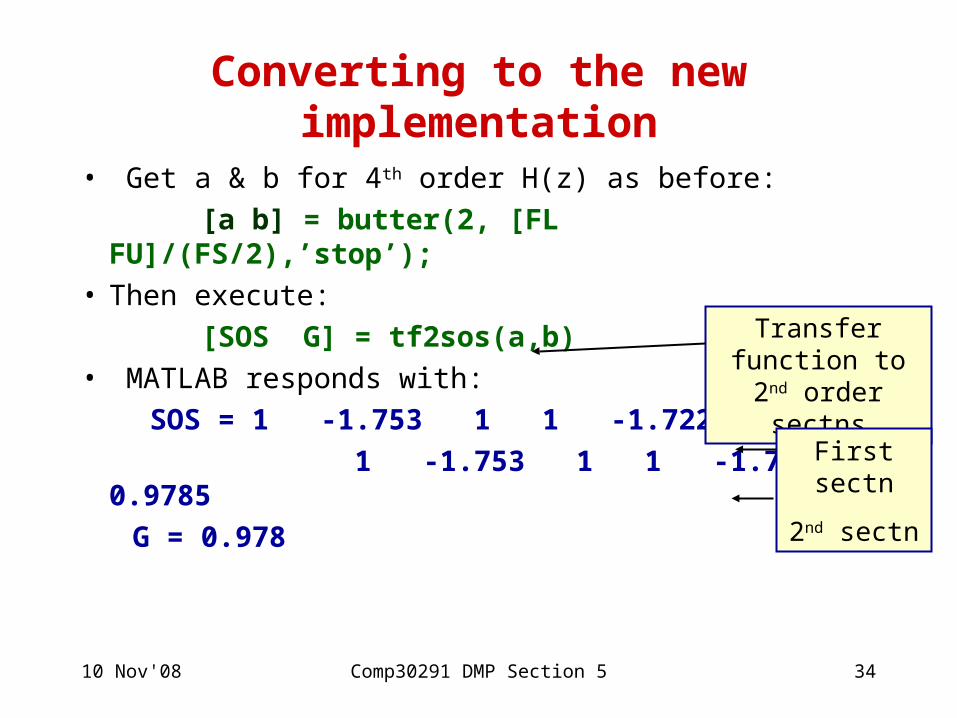
Converting to the new implementation
• Get a & b for 4th order H(z) as before:
[a b] = butter(2, [FL FU]/(FS/2),’stop’);• Then execute:
[SOS G] = tf2sos(a,b) • MATLAB responds with:
SOS = 1 -1.753 1 1 -1.722 0.9776
1 -1.753 1 1 -1.744 0.9785
G = 0.978
Transfer function to 2nd order sectns
First sectn
2nd sectn

10 Nov'08 Comp30291 DMP Section 5 35
H(z) may now be realised as:
x[n] 0.978
-1.753
1.722
-0.978
y[n]
-1.7531.744
-0.979
Fourth order IIR notch filter realised as two biquad (SOS) sections
10 Nov'08 Comp30291 DMP Section 5 36
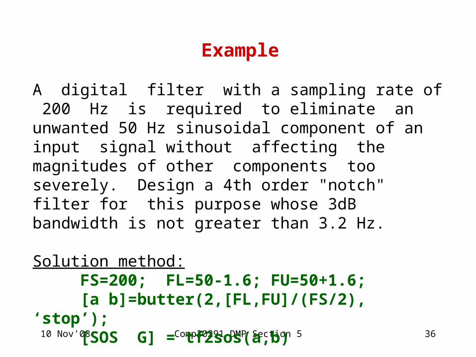
Example
A digital filter with a sampling rate of 200 Hz is required to eliminate an unwanted 50 Hz sinusoidal component of an input signal without affecting the magnitudes of other components too severely. Design a 4th order "notch" filter for this purpose whose 3dB bandwidth is not greater than 3.2 Hz.
Solution method:FS=200; FL=50-1.6; FU=50+1.6;[a b]=butter(2,[FL,FU]/(FS/2), ‘stop’);[SOS G] = tf2sos(a,b)
10 Nov'08 Comp30291 DMP Section 5 37
• Many design techniques for IIR digital filters have adopted ideas of analogue filters.
• Can transform analogue ‘prototype’ transfer function Ha(s) into H(z) for an IIR digital filter. • Analogue filters have infinite impulse-responses.
• Many gain-response approximations exist which are realisable by analogue filters
• e.g. Butterworth low-pass approximation which can be transformed to high-pass, band-pass & band-stop.
IIR digital filter design by bilinear transformation
10 Nov'08 Comp30291 DMP Section 5 38
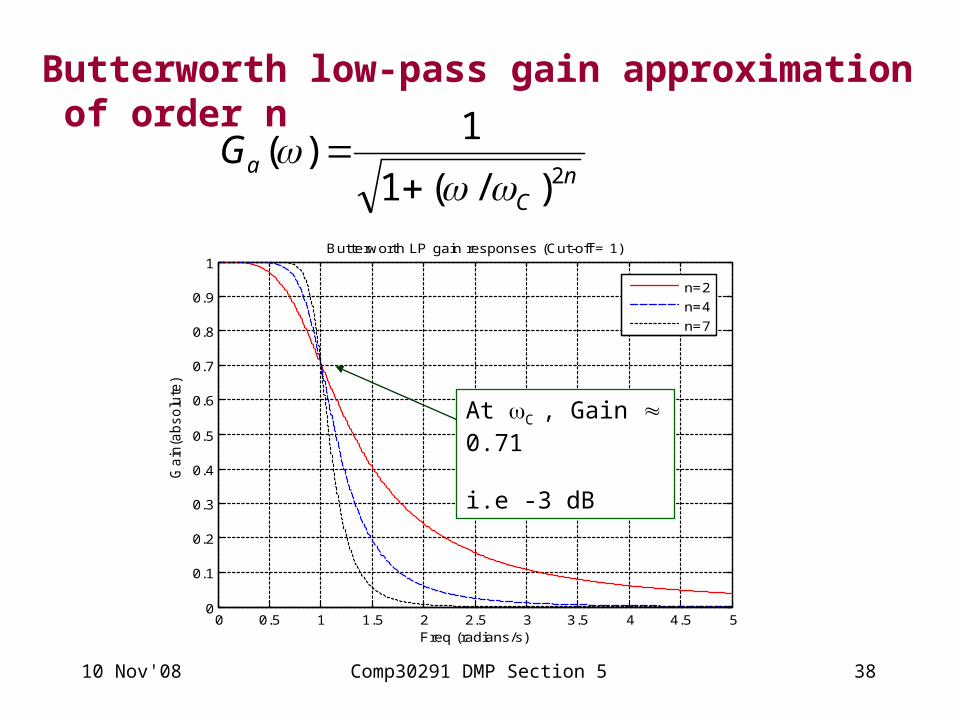
Butterworth low-pass gain approximation of order n
nC
aG2)/(1
1)(
0 0.5 1 1.5 2 2.5 3 3.5 4 4.5 50
0.1
0.2
0.3
0.4
0.5
0.6
0.7
0.8
0.9
1
Freq (radians/s)
Ga
in(a
bs
olu
te)
Butterworth LP gain responses (Cut-off = 1)
n=2
n=4
n=7
At C , Gain 0.71 i.e -3 dB
10 Nov'08 Comp30291 DMP Section 5 39
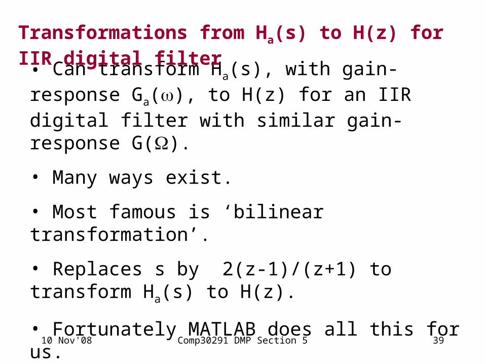
• Can transform Ha(s), with gain-response Ga(), to H(z) for an IIR digital filter with similar gain-response G().
• Many ways exist.
• Most famous is ‘bilinear transformation’.
• Replaces s by 2(z-1)/(z+1) to transform Ha(s) to H(z).
• Fortunately MATLAB does all this for us.
Transformations from Ha(s) to H(z) for IIR digital filter
10 Nov'08 Comp30291 DMP Section 5 40
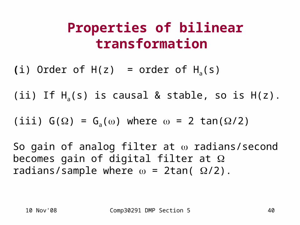
Properties of bilinear transformation
(i) Order of H(z) = order of Ha(s)
(ii) If Ha(s) is causal & stable, so is H(z).
(iii) G() = Ga() where = 2 tan(/2)
So gain of analog filter at radians/second becomes gain of digital filter at radians/sample where = 2tan( /2).
10 Nov'08 Comp30291 DMP Section 5 41
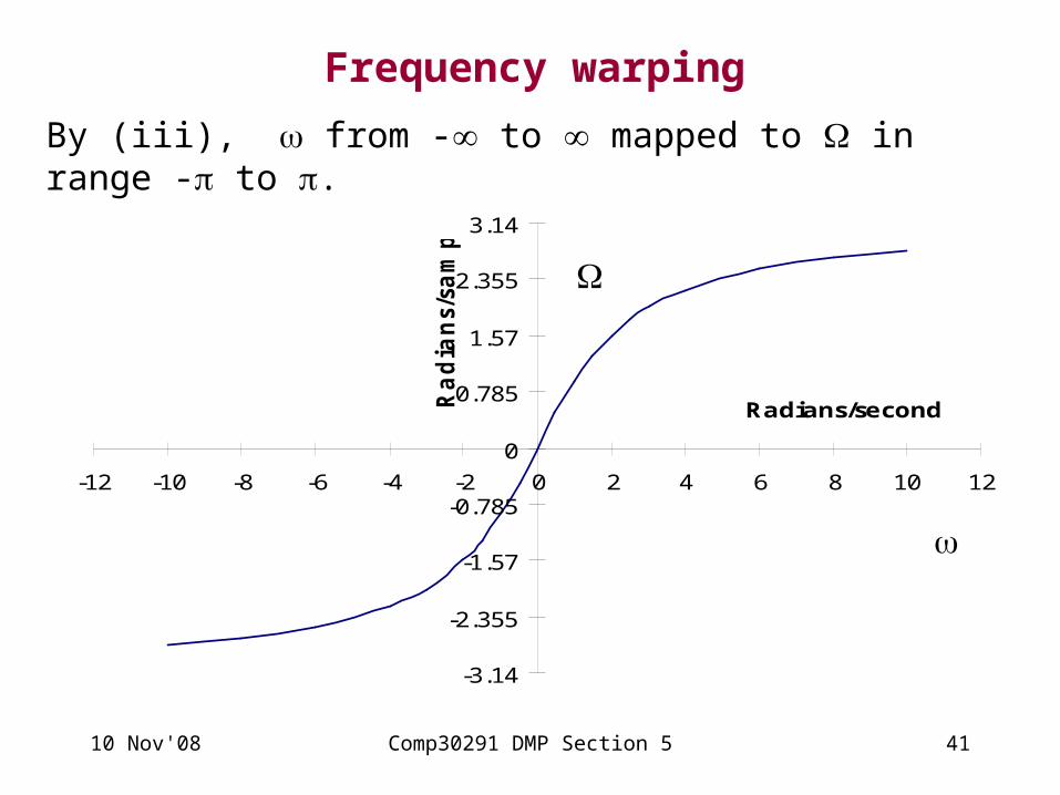
Frequency warping
By (iii), from - to mapped to in range - to .
-3.14
-2.355
-1.57
-0.785
0
0.785
1.57
2.355
3.14
-12 -10 -8 -6 -4 -2 0 2 4 6 8 10 12
Radians/secondRa
dia
ns/
sam
ple

10 Nov'08 Comp30291 DMP Section 5 42
• Shape of G() will change under the transformation.
• If Ga() is Butterworth, G() will not have exactly the same shape, but we still call it Butterworth.
• Mapping approx linear for in the range -2 to 2.
• As increases above 2 , a given increase in produces smaller and smaller increases in .
Frequency warping (cont)

10 Nov'08 Comp30291 DMP Section 5 43
• G() becomes more and more compressed as .
• Illustrate for an analog gain-response with ripples:
(a): Analogue gain response (b): Effect of bilinear transformation
Ga() G()
Comparing Ga() with G()

10 Nov'08 Comp30291 DMP Section 5 44
‘Prototype’ analogue transfer function
• Although the shape changes, we would like G() at its cut off C to the same as Ga() at its cut-off frequency.
• If Ga() is Butterworth, it is -3dB at its cut-off freq
• So we would like G() to be -3 dB at its cut-off C.
• Achieved if analogue prototype is designed to have its cut-off frequency at C = 2 tan(C/2).
C is the ‘pre-warped’ cut-off frequency.
• Designing analog prototype with cut-off freq 2 tan(C/2) guarantees that the digital filter will have its cut-off at C.
10 Nov'08 Comp30291 DMP Section 5 45
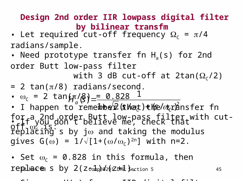
• Let required cut-off frequency C = /4 radians/sample.• Need prototype transfer fn Ha(s) for 2nd order Butt low-pass filter with 3 dB cut-off at 2tan(C/2) = 2 tan(/8) radians/second.• C = 2 tan(/8) = 0.828• I happen to remember that the transfer fn for a 2nd order Butt low-pass filter with cut-off C is:
2)/()/(21
1)(
CC
ass
sH
• If you don’t believe me, check that replacing s by j and taking the modulus gives G() = 1/[1+(/C)2n] with n=2.
• Set C = 0.828 in this formula, then replace s by 2(z-1)/(z+1).
• Gives us H(z) for an IIR digital filter. That’s it!
Design 2nd order IIR lowpass digital filter by bilinear transfm
10 Nov'08 Comp30291 DMP Section 5 46
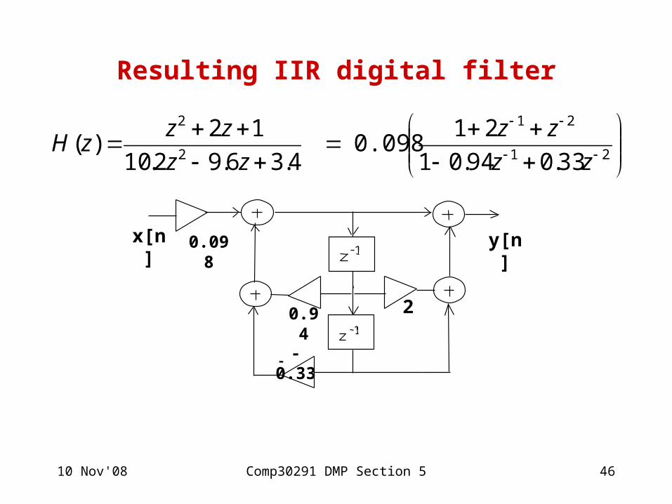
Resulting IIR digital filter
21
21
2
2
33.094.01
210.098
4.36.92.10
12)(
zz
zz
zz
zzzH
x[n] y[n]0.098
2 0.94
--0.33

10 Nov'08 Comp30291 DMP Section 5 47
Design of 2nd order IIR low-pass digital filter by bilinear transform using MATLAB
• If required cut-off freq is /4 radians/sample, type: [a b] = butter(2, 0.25)• MATLAB gives us:
a = [0.098 0.196 0.098]b = [1 -0.94 0.33]
The required expression for H(z) is therefore:
21
21
33.094.01
098.0196.0098.0)(
zz
zzzH
21
21
33.094.01
2 1 098.0 )(
zz
zzzH
To save multipliers it is a good idea to re-express this as:

10 Nov'08 Comp30291 DMP Section 5 48
Realise by ‘direct form 2’ signal-flow graph
21
21
33.094.01
21098.0
zz
zzzH
x[n] y[n] 0.098
2 0.94
-0.33
10 Nov'08 Comp30291 DMP Section 5 49
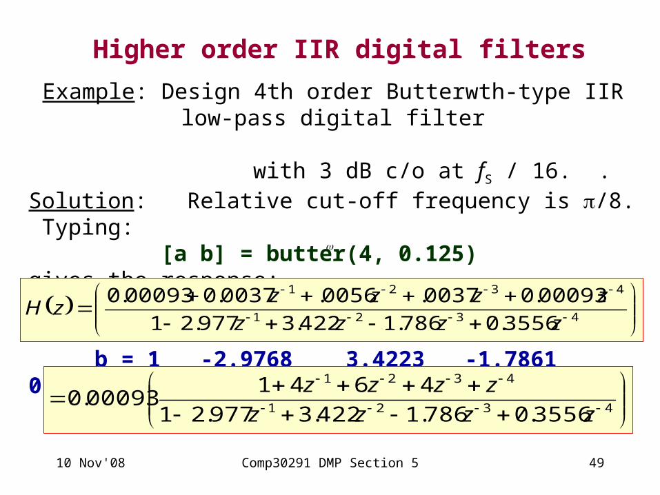
Higher order IIR digital filters
Example: Design 4th order Butterwth-type IIR low-pass digital filter with 3 dB c/o at fS / 16. .
Solution: Relative cut-off frequency is /8. Typing:[a b] = butter(4, 0.125)
gives the response:a = 0.0009 0.0037 0.0056 0.0037 0.0009b = 1 -2.9768 3.4223 -1.7861 0.3556
4321
4321
3556.0786.1422.3977.21
00093.00037.0056.0037.000093.0
zzzz
zzzzzH
4321
4321
3556.0786.1422.3977.21
464100093.0
zzzz
zzzz
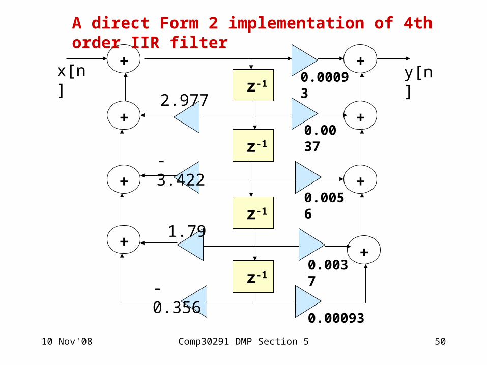
10 Nov'08 Comp30291 DMP Section 5 50
z-1
z-1
z-1
z-1
+
+
+
+
+
+
+
+
0.00093
2.977
-3.422
1.79
-0.356
0.00093
x[n] y[n]
0.0037
0.0056
0.0037
A direct Form 2 implementation of 4th order IIR filter

10 Nov'08 Comp30291 DMP Section 5 51
0.00093x[n]
z-1
z-1
z-1
z-1
+
+
+
+
+
+
+
+2.977
-3.422
1.79
-0.356
y[n]
4
6
4
Better ‘direct Form 2’ implementation of 4th order IIR filter
10 Nov'08 Comp30291 DMP Section 5 52
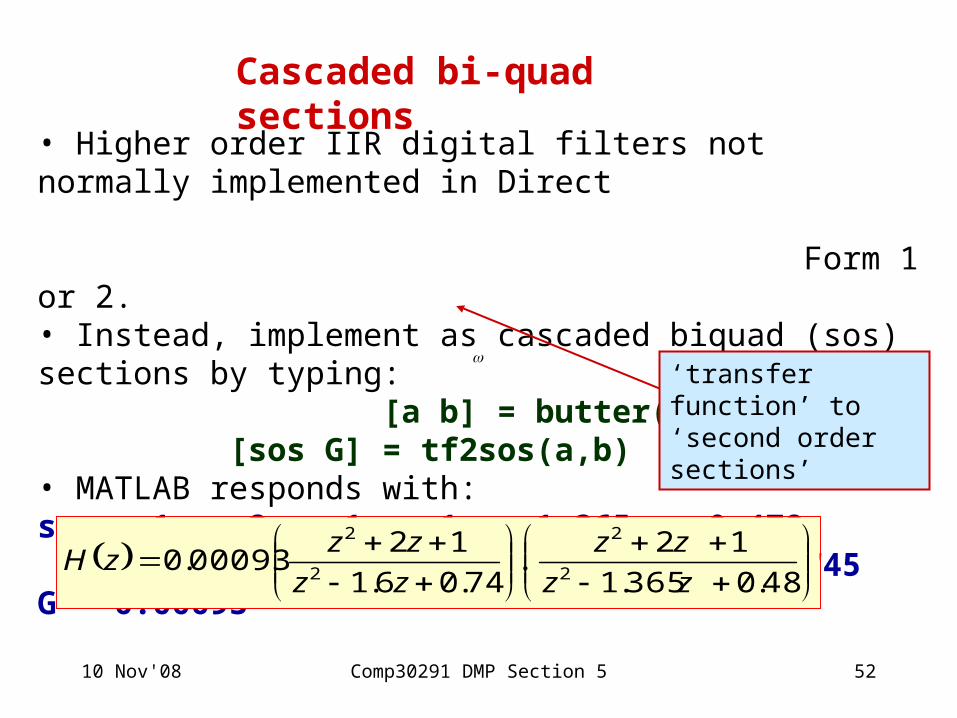
• Higher order IIR digital filters not normally implemented in Direct Form 1 or 2.• Instead, implement as cascaded biquad (sos) sections by typing: [a b] = butter(4, 0.125);
[sos G] = tf2sos(a,b) • MATLAB responds with:sos = 1 2 1 1 -1.365 0.478 1 2 1 1 -1.612 0.745G = 0.00093
48.0365.1
12.
74.06.1
1200093.0
2
2
2
2
zz
zz
zz
zzzH
Cascaded bi-quad sections
‘transfer function’ to ‘second order sections’

10 Nov'08 Comp30291 DMP Section 5 53
H(z) may be realised as:
x[n] 0.00093
2 1.6
-0.74
y[n]
2 1.36
-0.48
Fourth order IIR Butterworth filter with cut -off fs/16
10 Nov'08 Comp30291 DMP Section 5 54
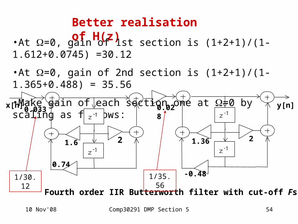
Better realisation of H(z)
•At =0, gain of 1st section is (1+2+1)/(1-1.612+0.0745) =30.12
•At =0, gain of 2nd section is (1+2+1)/(1-1.365+0.488) = 35.56
•Make gain of each section one at =0 by scaling as follows:
Fourth order IIR Butterworth filter with cut-off Fs/16
x[n] 0.033
2 1.6
-0.74
0.028 y[n]
2 1.36
-0.48
1/30.12 1/35.56

10 Nov'08 Comp30291 DMP Section 5 55
Analogue gain resp.
-0.1
0.1
0.3
0.5
0.7
0.9
1.1
0 0.5 1 1.5 2 2.5 3 3.5 4 4.5
Radians/second
Ga
in
Gain response of 4th order IIR filter
-0.1
0.1
0.3
0.5
0.7
0.9
1.1
0 0.785 1.57 2.355 3.14
Radians/sample
Ga
in
Gain-responses for 4th order analog & IIR digital filter
10 Nov'08 Comp30291 DMP Section 5 56
Compare gain-response of 4th order Butt low-pass transfer function used as a prototype, with that of derived digital filter.
• Both are 1 (0 dB) at zero frequency.• Both are 0.707 (-3 dB) at the cut-off frequency.
• Analogue gain approaches 0 as whereas digital filter gain becomes exactly zero at = .
• Shape of Butt gain response is "warped" by bilinear transfn.
• For digital filter, cut-off rate becomes sharper as because of the compression as .
10 Nov'08 Comp30291 DMP Section 5 57
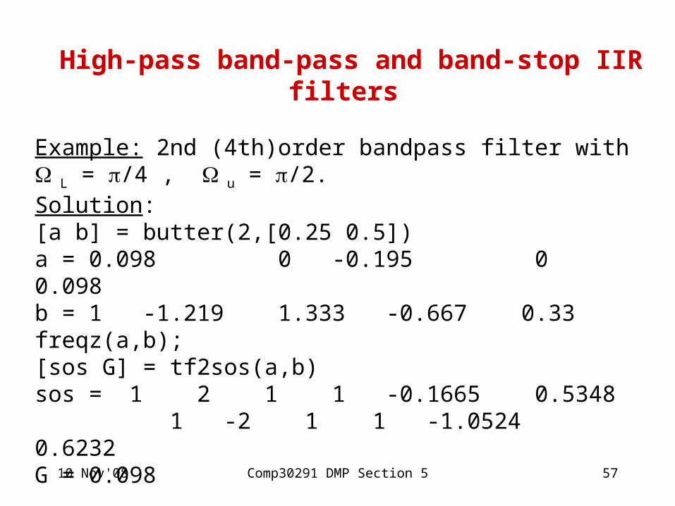
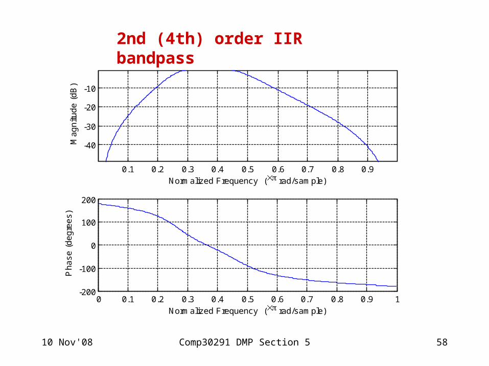
High-pass band-pass and band-stop IIR filters
Example: 2nd (4th)order bandpass filter with L = /4 , u = /2.Solution: [a b] = butter(2,[0.25 0.5])a = 0.098 0 -0.195 0 0.098b = 1 -1.219 1.333 -0.667 0.33freqz(a,b);[sos G] = tf2sos(a,b)sos = 1 2 1 1 -0.1665 0.5348 1 -2 1 1 -1.0524 0.6232G = 0.098
Many people call this 4th order - MATLAB calls it 2nd order.
10 Nov'08 Comp30291 DMP Section 5 58
0 0.1 0.2 0.3 0.4 0.5 0.6 0.7 0.8 0.9 1-200
-100
0
100
200
Normalized Frequency ( rad/sample)
Ph
as
e (
de
gre
es
)
0.1 0.2 0.3 0.4 0.5 0.6 0.7 0.8 0.9
-40
-30
-20
-10
Normalized Frequency ( rad/sample)
Ma
gn
itu
de
(d
B)
2nd (4th) order IIR bandpass

10 Nov'08 Comp30291 DMP Section 5 59
Arranged as 2 biquad sections
21
21
11
21
62.005.11
21
54.017.01
211.0)(
zz
zz
zz
zzzH
x[n] 0.1
-2 .17
-0.54
1 y[n]
2 1.05
-0.62
10 Nov'08 Comp30291 DMP Section 5 60
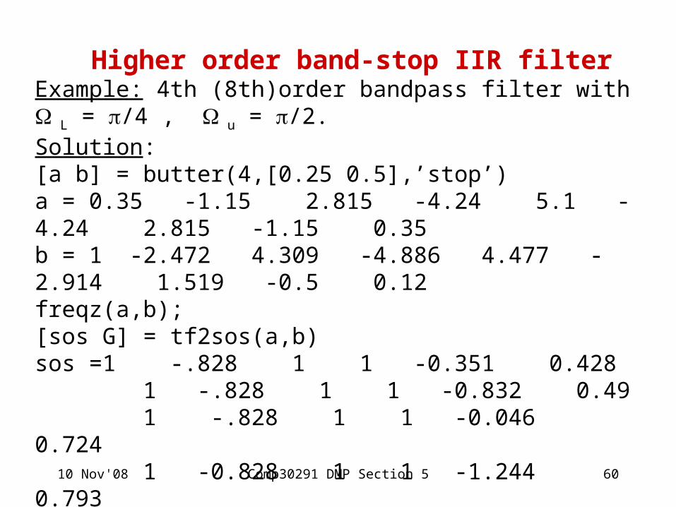
Higher order band-stop IIR filterExample: 4th (8th)order bandpass filter with L = /4 , u = /2.Solution: [a b] = butter(4,[0.25 0.5],’stop’)a = 0.35 -1.15 2.815 -4.24 5.1 -4.24 2.815 -1.15 0.35b = 1 -2.472 4.309 -4.886 4.477 -2.914 1.519 -0.5 0.12freqz(a,b);[sos G] = tf2sos(a,b)sos =1 -.828 1 1 -0.351 0.428 1 -.828 1 1 -0.832 0.49 1 -.828 1 1 -0.046 0.724 1 -0.828 1 1 -1.244 0.793G = 0.347

10 Nov'08 Comp30291 DMP Section 5 61
Gain & phase resp of IIR band-stop filter
0 0.1 0.2 0.3 0.4 0.5 0.6 0.7 0.8 0.9 1-800
-600
-400
-200
0
Normalized Frequency ( rad/sample)
Ph
as
e (
de
gre
es
)
0 0.1 0.2 0.3 0.4 0.5 0.6 0.7 0.8 0.9 1-40
-30
-20
-10
0
Normalized Frequency ( rad/sample)
Ma
gn
itu
de
(d
B)
10 Nov'08 Comp30291 DMP Section 5 62
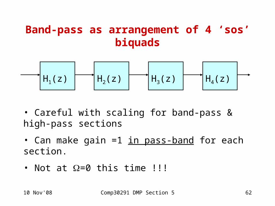
Band-pass as arrangement of 4 ‘sos’ biquads
H1(z) H2(z) H3(z) H4(z)
• Careful with scaling for band-pass & high-pass sections
• Can make gain =1 in pass-band for each section.
• Not at =0 this time !!!

10 Nov'08 Comp30291 DMP Section 5 63
•. Must use
[sos G] = tf2sos ([a4 a3 a2 a1 a0], [b4 … b0 ])
• ‘help tf2sos’ to find out abt this function
Transfer-function to second order sections: ‘tf2sos’
10 Nov'08 Comp30291 DMP Section 5 64
•Option of cascading high pass & low-pass digital filters to give band-pass or band-stop filters must be used with care.
•It is much simpler & avoids the factorisation problem.
•Then make sure that analogue prototype is wide-band
• High-pass IIR filters are designed by:
[a b] = butter(4,0.125,’high’);
Wide-band band-pass & band-stop filters
10 Nov'08 Comp30291 DMP Section 5 65
Comparison of IIR and FIR digital filters
Advantage of IIR type digital filters:
Economical in use of delays, multipliers and adders.
Disadvantages:
(1) Sensitive to coefficient round-off inaccuracies & effects of overflow in fixed point arith. These effects can lead to instability or serious distortion.
(2) An IIR filter cannot be exactly linear phase.
10 Nov'08 Comp30291 DMP Section 5 66
Advantages of FIR filters:
(1) may be realised by non-recursive structures which are simpler and more convenient for programming especially on devices specifically designed for DSP. (2) FIR structures are always stable.(3) Because there is no recursion, round-off and overflow errors are easily controlled. (4) An FIR filter can be exactly linear phase.
Disadvantage of FIR filters:
Large orders can be required to perform fairly simple filtering tasks.

10 Nov'08 Comp30291 DMP Section 5 67
Problems 1 Find H(z) for the following difference equations
(a) y[n] = 2x[n] - 3x[n-1] + 6x[n-4] (b) y[n] = x[n-1] - y[n-1] - 0.5y[n-2]
2 Show that passing {x[n]} thro’ H(z) = z - 1 produces {x[n-1]}.3. Give difference equation & give a signal-flow graph for: 1 + 3 z - 1 + 2z - 2
H(z) = 1 + 0.9z - 1
Plot poles & zeros & roughly sketch its gain response.4 Calculate the impulse response of the digital filter with
1 H(z) = 1 - 2 z - 1
Draw its signal flow graph, plot its poles and zeros and comment on them.5. Plot poles & zeros for the following difference equation: y[n] = x[n] - 0.9x[n-1] + 0.81x[n-2] + 0.95y[n-1] - 0.9025y[n-2] on z-plane and estimate gain and phase responses

10 Nov'08 Comp30291 DMP Section 5 68
6 Write high level language program, or give flow diagram to implement difference equation given in Prob. 2.6.7. Modify your program for prob 7 so that it uses only integers.8. If LTI systems L1 & L2, with imp-responses {h1[n]} & {h2[n]} are arranged as below, calculate overall impulse- response. Show that this is affected by interchanging L1 & L2 .
L 1 L 2 x[n] y[n]
{ h 1 [n] } { h 2 [n] }
9. A 3rd order low-pass IIR filter is required with 3 dB cut-off at f S /4. Apply bilinear transfn to design it & give its signal flow graph as 2nd & 1st order sections in cascade. 10. Give program to implement 3rd order IIR filter above in floating point arithmetic. Then do it in fixed point arithmetic.11. Low-pass IIR digital filter required with cut-off at f s/4 & stop-band attenuation at least 20 dB for all frequencies above 3f s /8 & below f s /2. Design by bilinear transfn using MATLAB.

10 Nov'08 Comp30291 DMP Section 5 69
12. Design a 4th order band-pass IIR digital filter with lower & upper cut-off frequencies at 300 Hz & 3400 Hz when fS = 8 kHz.13. Design a 4th order band-pass IIR digital filter with lower & upper cut-off frequencies at 2000 Hz & 3000 Hz when fS = 8 kHz.14. What limits how good a notch filter we can implement on a fixed point DSP processor? In theory we can make notch sharper & sharper by moving poles closer & closer to zeros. What limits us in practice. I wonder how sharp a notch we could get in 16-bit fixed pt arithmetic?15. What order of FIR filter would be required to implement a /4 notch approximately as good as a 2nd order IIR /4 notch with 3 dB bandwidth 0.2 radians/sample?16. What order of FIR low-pass filter would be required to be approx as good as the 2nd order IIR low-pass filter (/4 cut-off) designed in these notes?
Related Documents