1 Unit-01/Lecture-01 Introduction to Algorithms, Designing ...

UNIT – 1

Unit-01/Lecture-01

Introduction to Algorithms, Designing algorithms

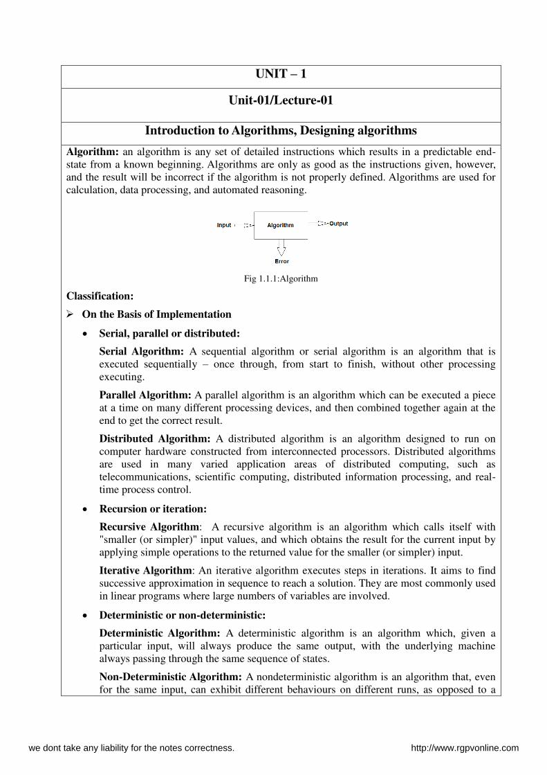
Algorithm: an algorithm is any set of detailed instructions which results in a predictable end-state from a known beginning. Algorithms are only as good as the instructions given, however, and the result will be incorrect if the algorithm is not properly defined. Algorithms are used for calculation, data processing, and automated reasoning.

Fig 1.1.1:Algorithm

Classification:

On the Basis of Implementation

Serial, parallel or distributed:

Serial Algorithm: A sequential algorithm or serial algorithm is an algorithm that is executed sequentially – once through, from start to finish, without other processing executing.

Parallel Algorithm: A parallel algorithm is an algorithm which can be executed a piece at a time on many different processing devices, and then combined together again at the end to get the correct result.

Distributed Algorithm: A distributed algorithm is an algorithm designed to run on computer hardware constructed from interconnected processors. Distributed algorithms are used in many varied application areas of distributed computing, such as telecommunications, scientific computing, distributed information processing, and real-time process control.

Recursion or iteration:

Recursive Algorithm: A recursive algorithm is an algorithm which calls itself with "smaller (or simpler)" input values, and which obtains the result for the current input by applying simple operations to the returned value for the smaller (or simpler) input.

Iterative Algorithm: An iterative algorithm executes steps in iterations. It aims to find successive approximation in sequence to reach a solution. They are most commonly used in linear programs where large numbers of variables are involved.

Deterministic or non-deterministic:

Deterministic Algorithm: A deterministic algorithm is an algorithm which, given a particular input, will always produce the same output, with the underlying machine always passing through the same sequence of states.

Non-Deterministic Algorithm: A nondeterministic algorithm is an algorithm that, even for the same input, can exhibit different behaviours on different runs, as opposed to a

we dont take any liability for the notes correctness. http://www.rgpvonline.com

deterministic algorithm. Exact or approximate

On the Basis of Design

Divide and conquer: A divide and conquer algorithm repeatedly reduces an instance of a problem to one or more smaller instances of the same problem (usually recursively) until the instances are small enough to solve easily.

Dynamic programming: It is a method for efficiently solving a broad range of search and optimization problems which exhibit the characteristics of overlapping sub problems and optimal substructure.

Greedy Algorithms: A greedy algorithm is a mathematical process that looks for simple, easy-to-implement solutions to complex, multi-step problems by deciding which next step will provide the most obvious benefit. Such algorithms are called greedy because while the optimal solution to each smaller instance will provide an immediate output, the algorithm doesn’t consider the larger problem as a whole. Once a decision has been made, it is never reconsidered.

Backtracking Algorithm: Backtracking is a general algorithm for finding all (or some) solutions to some computational problems, notably constraint satisfaction problems, that incrementally builds candidates to the solutions, and abandons each partial candidate c ("backtracks") as soon as it determines that c cannot possibly be completed to a valid solution.

Branch & Bound: Branch and bound algorithms are a variety of adaptive partition strategies have been proposed to solve global optimization models. These are based upon partition, sampling, and subsequent lower and upper bounding procedures

S.NO

RGPV QUESTIONS Year Marks

Q.1 Q.2

Unit-01/Lecture-02

Analyzing algorithms, Step Count and Complexity


Why Analyze an Algorithm?

The most straightforward reason for analyzing an algorithm is to discover its characteristics in order to evaluate its suitability for various applications or compare it with other algorithms for the same application. Moreover, the analysis of an algorithm can help us understand it better, and can suggest informed improvements. Algorithms tend to become shorter, simpler, and more elegant during the analysis process.

Computational Complexity:

The branch of theoretical computer science where the goal is to classify algorithms according to their efficiency and computational problems according to their inherent difficulty is known as computational complexity. Paradoxically, such classifications are typically not useful for predicting performance or for comparing algorithms in practical applications because they focus on order-of-growth worst-case performance. In this book, we focus on analyses that can be used to predict performance and compare algorithms.

Analysis of Algorithms:

A complete analysis of the running time of an algorithm involves the following steps:

Implement the algorithm completely.

Determine the time required for each basic operation.

Identify unknown quantities that can be used to describe the frequency of execution of the basic operations.

Develop a realistic model for the input to the program.

Analyze the unknown quantities, assuming the modelled input.

Calculate the total running time by multiplying the time by the frequency for each operation, then adding all the products.

Complexity of An Algorithm:

Time Complexity: The time complexity of an algorithm quantifies the amount of time taken by an algorithm to run. It is commonly estimated by counting the number of elementary operations performed by the algorithm, where an elementary operation takes a fixed amount of time to perform.

Space Complexity: This is essentially the number of memory cells which an algorithm needs to run. A good algorithm keeps this number as small as possible.

There is often a time-space trade-off involved in a problem, that is, it cannot be solved with few computing time and low memory consumption. One then has to make a compromise and to exchange computing time for memory consumption or vice versa, depending on which algorithm one chooses and how one parameterizes it.

Amortized analysis:

Sometimes we find the statement in the manual that an operation takes amortized time O(f(n)). This means that the total time for n such operations is bounded asymptotically from above by a function g(n) and that f(n)=O(g(n)/n). So the amortized time is (a bound for) the average time of an operation in the worst case.

Step Count:

• s/e is the number of steps per execution of the statement.


• Frequency is how often each statement is executed.

• The time complexity is estimated as Total steps.

Statement S/e Frequency Total

1. Algorithm Sum(a,n) 2.{ 3. S=0.0; 4. for I=1 to n do 5. s=s+a[I]; 6. return s; 7. }

0 0 1 1 1 1 0

- - 1

n+1 n 1 -

0 0 1

n+1 n 1 0

Total 2n+3

Table 1.2.1: Step Count of Sequential Search

Worst-case complexity: The worst-case complexity of the algorithm is the function defined by the maximum number of steps taken on any instance of size n. It represents the curve passing through the highest point of each column.

Best-case complexity: The best-case complexity of the algorithm is the function defined by the minimum number of steps taken on any instance of size n. It represents the curve passing through the lowest point of each column.

Average-case complexity: The average-case complexity of the algorithm is the function defined by the average number of steps taken on any instance of size n.

Asymptotic Notations:

The goal of computational complexity is to classify algorithms according to their performances.

Definition of "big Oh"

For any monotonic functions f(n) and g(n) from the positive integers to the positive integers, we say that f(n) = O(g(n)) when there exist constants c > 0 and n0 > 0 such that

f(n) ≤ c * g(n), for all n ≥ n0

Intuitively, this means that function f(n) does not grow faster than g(n), or that function g(n) is an upper bound for f(n), for all sufficiently large n→∞

Here is a graphic representation of f(n) = O(g(n)) relation:

Fig 1.2.1: Graph of Big Oh Notation


Examples:

Constant Time: O(1)

Linear Time: O(n)

Logarithmic Time: O(log n)

Quadratic Time: O(n2)

Definition of "big Omega":

We need the notation for the lower bound. A capital omega Ω notation is used in this case. We say that f(n) = Ω(g(n)) when there exist constant c that f(n) ≥ c*g(n) for for all sufficiently large n. Examples

Constant Time: Ω(1)

Linear Time: Ω(n)

Logarithmic Time: Ω(log n)

Quadratic Time: Ω(n2)

Definition of "big Theta":

To measure the complexity of a particular algorithm, means to find the upper and lower bounds. A new notation is used in this case. We say that f(n) = Θ(g(n)) if and only f(n) = O(g(n)) and f(n) = Ω(g(n)).

Examples

Constant Time: Θ(1)

Linear Time: Θ(n)

Logarithmic Time: Θ(log n)

Quadratic Time: Θ(n2)

S.NO


Q.1 What are different asymptotic notations used? Explain. 2014 2 Q.2 Describe the methods of analyzing an algorithm. What do you mean

by best case, average case and worst case time complexity of an

algorithm?

2013 7

Q.3

Unit-01/Lecture-03

Heap and Heap Sort


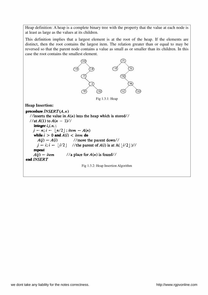
Heap definition: A heap is a complete binary tree with the property that the value at each node is at least as large as the values at its children.

This definition implies that a largest element is at the root of the heap. If the elements are distinct, then the root contains the largest item. The relation greater than or equal to may be reversed so that the parent node contains a value as small as or smaller than its children. In this case the root contains the smallest element.

Fig 1.3.1: Heap

Heap Insertion:

Fig 1.3.2: Heap Insertion Algorithm


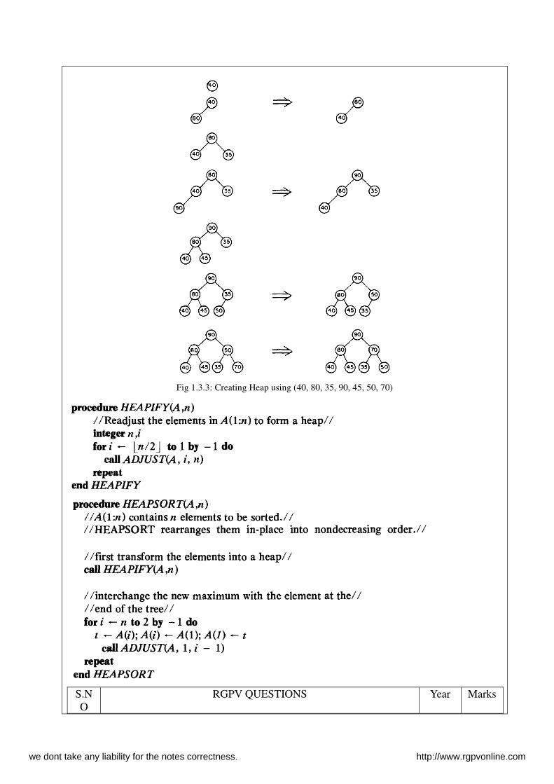
Fig 1.3.3: Creating Heap using (40, 80, 35, 90, 45, 50, 70)

S.NO



Q.1 Following nodes are inserted in empty tree to form minimum heap with neat sketches show how insertion will be done 8, 7, 11, 6, 2, 1, 5, 12.

2013 7

Q.2

Q.3

Unit-01/Lecture-04

Introduction to divide and conquer technique


DIVIDE AND CONQUER:

Given a function to compute on ‘n’ inputs the divide-and-conquer strategy suggests splitting the inputs into ‘k’ distinct subsets, 1<k<=n, yielding ‘k’ sub problems.

These sub problems must be solved, and then a method must be found to combine sub solutions into a solution of the whole.

If the sub problems are still relatively large, then the divide-and-conquer strategy can possibly be reapplied.

Often the sub problems resulting from a divide-and-conquer design are of the same type as the original problem.

For those cases the re application of the divide-and-conquer principle is naturally expressed by a recursive algorithm.

D And C(Algorithm) is initially invoked as D and C(P), where ‘p’ is the problem to be solved.

Small(P) is a Boolean-valued function that determines whether the i/p size is small enough that the answer can be computed without splitting.

If this so, the function ‘S’ is invoked.

Otherwise, the problem P is divided into smaller sub problems.

These sub problems P1, P2 …Pk are solved by recursive application of D And C.

Combine is a function that determines the solution to p using the solutions to the ‘k’ sub problems.

If the size of ‘p’ is n and the sizes of the ‘k’ sub problems are n1, n2 ….nk, respectively, then the computing time of D And C is described by the recurrence relation.

T(n)= g(n) n small

T(n1)+T(n2)+……………+T(nk)+f(n); otherwise.

Where T(n) is the time for D And C on any I/p of size ‘n’. g(n) is the time of compute the answer directly for small I/ps.

f(n) is the time for dividing P & combining the solution to sub problems.

Algorithm D And C(P)

{

if small(P) then return S(P);

else

{

divide P into smaller instances

P1, P2… Pk, k>=1; Apply D And C to each of these sub problems;

return combine (D And C(P1), D And C(P2),…….,D And C(Pk)); }

}


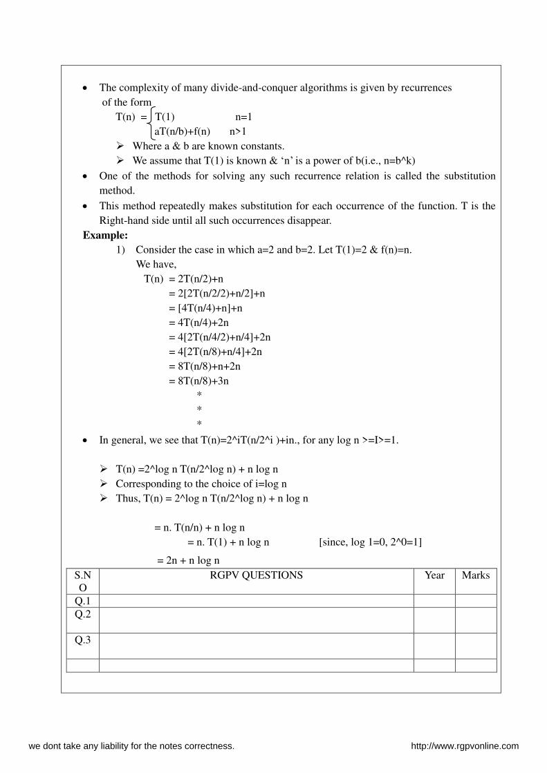
The complexity of many divide-and-conquer algorithms is given by recurrences

of the form

T(n) = T(1) n=1

aT(n/b)+f(n) n>1

Where a & b are known constants.

We assume that T(1) is known & ‘n’ is a power of b(i.e., n=b^k)

One of the methods for solving any such recurrence relation is called the substitution

method.

This method repeatedly makes substitution for each occurrence of the function. T is the

Right-hand side until all such occurrences disappear.

Example:

1) Consider the case in which a=2 and b=2. Let T(1)=2 & f(n)=n.

We have,

T(n) = 2T(n/2)+n

= 2[2T(n/2/2)+n/2]+n

= [4T(n/4)+n]+n

= 4T(n/4)+2n

= 4[2T(n/4/2)+n/4]+2n

= 4[2T(n/8)+n/4]+2n

= 8T(n/8)+n+2n

= 8T(n/8)+3n

*

*

*

In general, we see that T(n)=2^iT(n/2^i )+in., for any log n >=I>=1.

T(n) =2^log n T(n/2^log n) + n log n

Corresponding to the choice of i=log n

Thus, T(n) = 2^log n T(n/2^log n) + n log n

= n. T(n/n) + n log n

= n. T(1) + n log n [since, log 1=0, 2^0=1]

= 2n + n log n

S.NO


Q.1 Q.2

Q.3


Unit-01/Lecture-05

Recurrence Relation

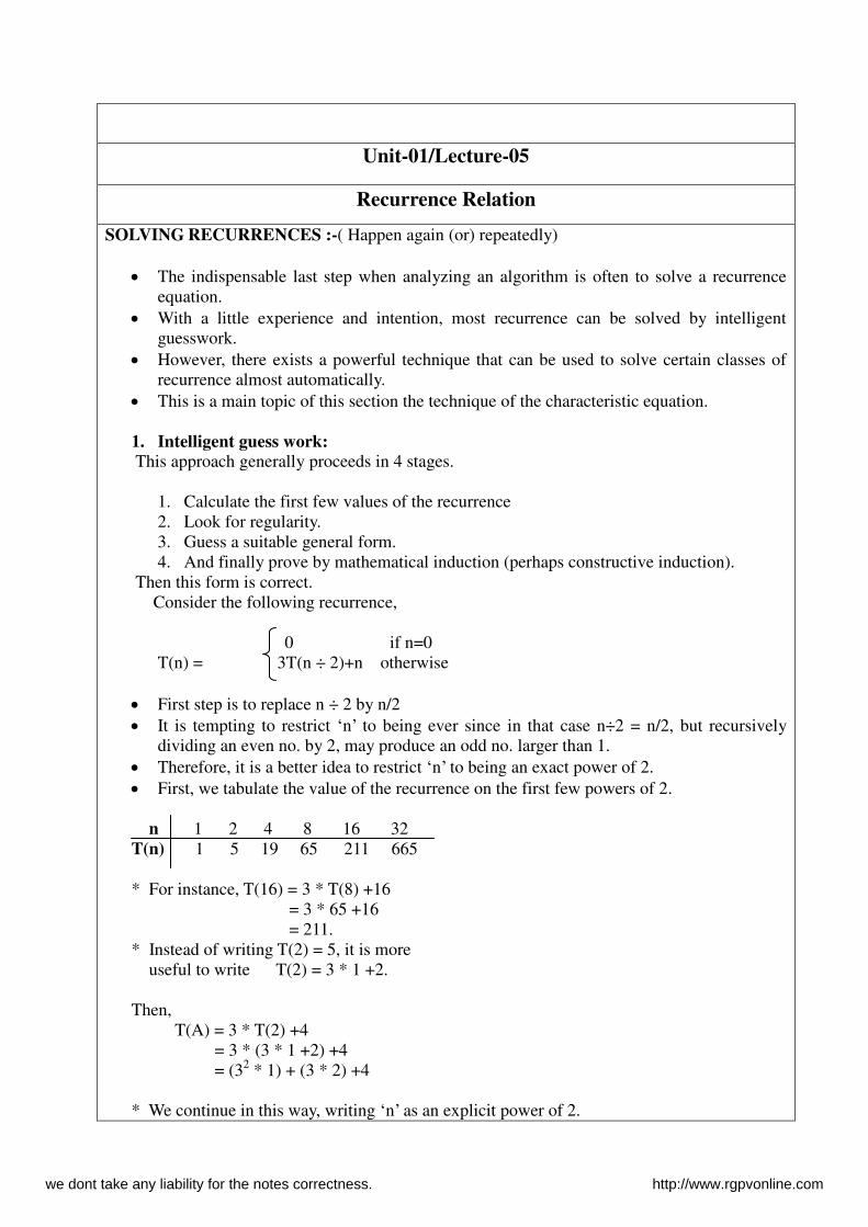
SOLVING RECURRENCES :-( Happen again (or) repeatedly)

The indispensable last step when analyzing an algorithm is often to solve a recurrence equation.

With a little experience and intention, most recurrence can be solved by intelligent guesswork.

However, there exists a powerful technique that can be used to solve certain classes of recurrence almost automatically.

This is a main topic of this section the technique of the characteristic equation. 1. Intelligent guess work:

This approach generally proceeds in 4 stages.

1. Calculate the first few values of the recurrence 2. Look for regularity. 3. Guess a suitable general form. 4. And finally prove by mathematical induction (perhaps constructive induction).

Then this form is correct. Consider the following recurrence, 0 if n=0 T(n) = 3T(n ÷ 2)+n otherwise

First step is to replace n ÷ 2 by n/2 It is tempting to restrict ‘n’ to being ever since in that case n÷2 = n/2, but recursively

dividing an even no. by 2, may produce an odd no. larger than 1. Therefore, it is a better idea to restrict ‘n’ to being an exact power of 2. First, we tabulate the value of the recurrence on the first few powers of 2. n 1 2 4 8 16 32 T(n) 1 5 19 65 211 665 * For instance, T(16) = 3 * T(8) +16 = 3 * 65 +16 = 211. * Instead of writing T(2) = 5, it is more useful to write T(2) = 3 * 1 +2. Then, T(A) = 3 * T(2) +4 = 3 * (3 * 1 +2) +4 = (32 * 1) + (3 * 2) +4 * We continue in this way, writing ‘n’ as an explicit power of 2.


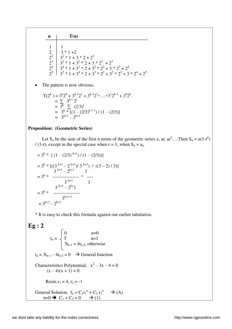
n T(n)

1 1 2 3 * 1 +2 22 32 * 1 + 3 * 2 + 22 23 33 * 1 + 32 * 2 + 3 * 22 + 23 24 34 * 1 + 33 * 2 + 32 * 22 + 3 * 23 + 24 25 35 * 1 + 34 * 2 + 33 * 22 + 32 * 23 + 3 * 24 + 25

The pattern is now obvious.

T(2k ) = 3k20 + 3k-121 + 3k-222+…+312k-1 + 302k. = ∑ 3k-i 2i = 3k ∑ (2/3)i = 3k * [(1 – (2/3)k + 1) / (1 – (2/3)] = 3k+1 – 2k+1

Proposition: (Geometric Series)

Let Sn be the sum of the first n terms of the geometric series a, ar, ar2….Then Sn = a(1-rn) / (1-r), except in the special case when r = 1; when Sn = an.

= 3k * [ (1 – (2/3) k+1) / (1 – (2/3))] = 3k * [((3 k+1 – 2 k+1)/ 3 k+1) / ((3 – 2) / 3)] 3 k+1 – 2k+1 3 = 3k * ----------------- * ---- 3 k+1 1 3 k+1 – 2k+1 = 3k * ----------------- 3k+1-1 = 3k+1 – 2k+1

* It is easy to check this formula against our earlier tabulation.

Eg : 2 0 n=0 tn = 5 n=1 3tn-1 + 4tn-2, otherwise tn = 3tn-1 – 4tn-2 = 0 General function Characteristics Polynomial, x2 – 3x – 4 = 0 (x – 4)(x + 1) = 0 Roots r1 = 4, r2 = -1 General Solution, fn = C1r1

n + C2 r2n (A)

n=0 C1 + C2 = 0 (1)


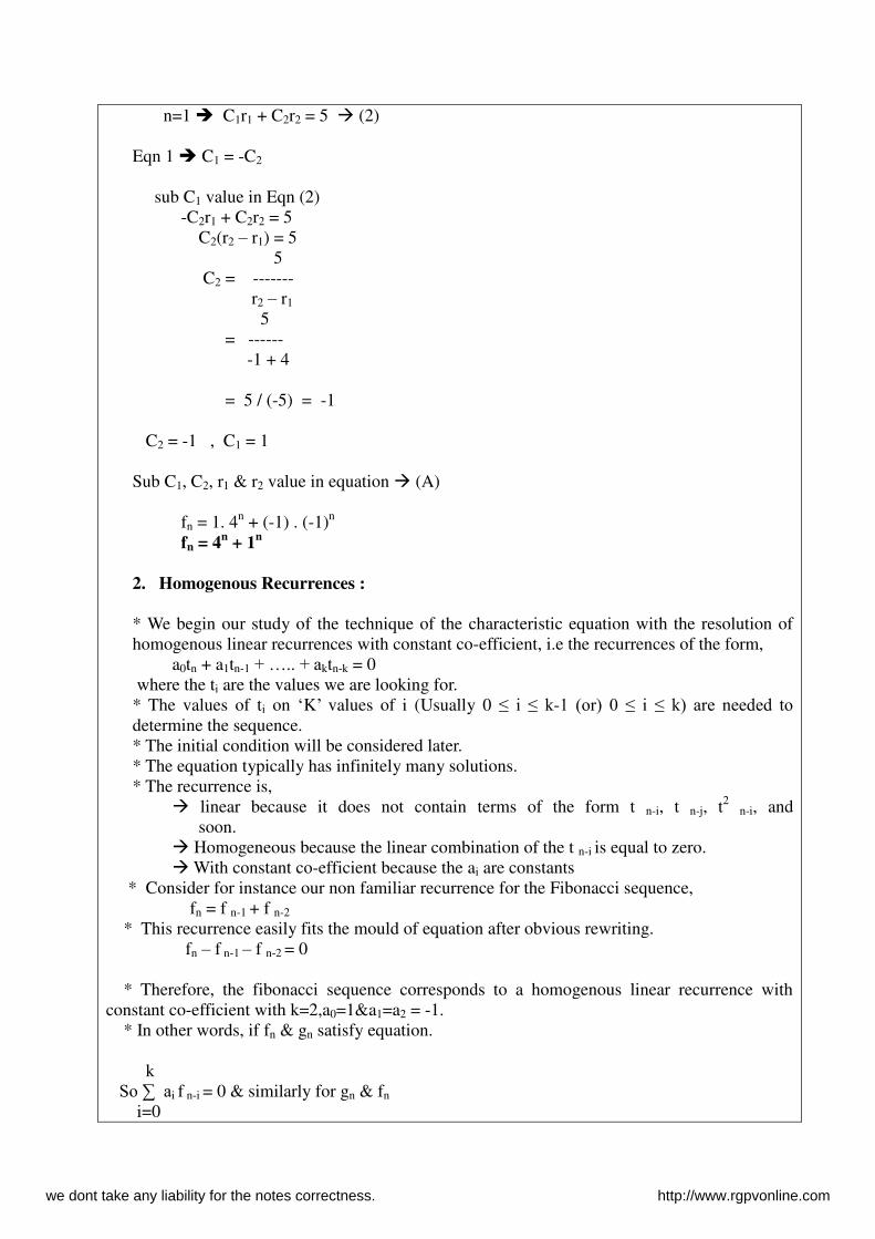
n=1 C1r1 + C2r2 = 5 (2) Eqn 1 C1 = -C2 sub C1 value in Eqn (2) -C2r1 + C2r2 = 5 C2(r2 – r1) = 5 5 C2 = ------- r2 – r1 5 = ------ -1 + 4 = 5 / (-5) = -1 C2 = -1 , C1 = 1 Sub C1, C2, r1 & r2 value in equation (A) fn = 1. 4n + (-1) . (-1)n fn = 4

n + 1

n

2. Homogenous Recurrences :

* We begin our study of the technique of the characteristic equation with the resolution of homogenous linear recurrences with constant co-efficient, i.e the recurrences of the form, a0tn + a1tn-1 + ….. + aktn-k = 0 where the ti are the values we are looking for. * The values of ti on ‘K’ values of i (Usually 0 ≤ i ≤ k-1 (or) 0 ≤ i ≤ k) are needed to determine the sequence. * The initial condition will be considered later.

* The equation typically has infinitely many solutions. * The recurrence is, linear because it does not contain terms of the form t n-i, t n-j, t2 n-i, and

soon. Homogeneous because the linear combination of the t n-i is equal to zero. With constant co-efficient because the ai are constants * Consider for instance our non familiar recurrence for the Fibonacci sequence, fn = f n-1 + f n-2

* This recurrence easily fits the mould of equation after obvious rewriting. fn – f n-1 – f n-2 = 0 * Therefore, the fibonacci sequence corresponds to a homogenous linear recurrence with constant co-efficient with k=2,a0=1&a1=a2 = -1. * In other words, if fn & gn satisfy equation. k So ∑ ai f n-i = 0 & similarly for gn & fn i=0


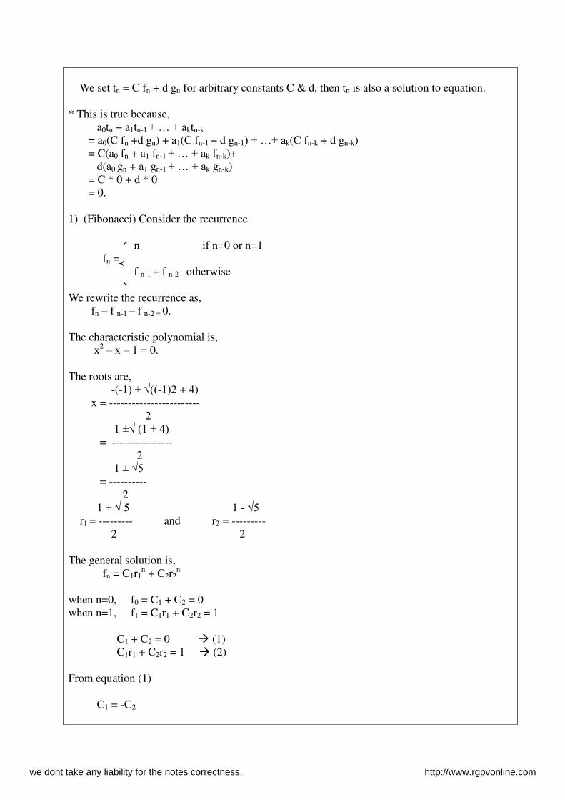
We set tn = C fn + d gn for arbitrary constants C & d, then tn is also a solution to equation. * This is true because, a0tn + a1tn-1 + … + aktn-k = a0(C fn +d gn) + a1(C fn-1 + d gn-1) + …+ ak(C fn-k + d gn-k) = C(a0 fn + a1 fn-1 + … + ak fn-k)+ d(a0 gn + a1 gn-1 + … + ak gn-k) = C * 0 + d * 0 = 0. 1) (Fibonacci) Consider the recurrence. n if n=0 or n=1 fn = f n-1 + f n-2 otherwise We rewrite the recurrence as, fn – f n-1 – f n-2 = 0. The characteristic polynomial is, x2 – x – 1 = 0. The roots are, -(-1) ± √((-1)2 + 4) x = ------------------------ 2 1 ±√ (1 + 4) = ---------------- 2 1 ± √5 = ---------- 2 1 + √ 5 1 - √5 r1 = --------- and r2 = --------- 2 2 The general solution is, fn = C1r1

n + C2r2n

when n=0, f0 = C1 + C2 = 0 when n=1, f1 = C1r1 + C2r2 = 1 C1 + C2 = 0 (1) C1r1 + C2r2 = 1 (2) From equation (1) C1 = -C2


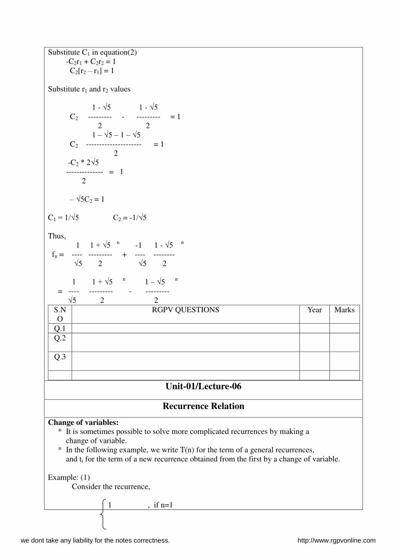
Substitute C1 in equation(2) -C2r1 + C2r2 = 1 C2[r2 – r1] = 1 Substitute r1 and r2 values 1 - √5 1 - √5 C2 --------- - --------- = 1 2 2 1 – √5 – 1 – √5 C2 --------------------- = 1 2 -C2 * 2√5 -------------- = 1 2 – √5C2 = 1 C1 = 1/√5 C2 = -1/√5 Thus, 1 1 + √5 n -1 1 - √5 n fn = ---- --------- + ---- -------- √5 2 √5 2 1 1 + √5 n 1 – √5 n = ---- --------- - --------- √5 2 2

S.NO


Q.1 Q.2

Q.3

Unit-01/Lecture-06

Recurrence Relation

Change of variables: * It is sometimes possible to solve more complicated recurrences by making a change of variable. * In the following example, we write T(n) for the term of a general recurrences, and ti for the term of a new recurrence obtained from the first by a change of variable. Example: (1) Consider the recurrence, 1 , if n=1


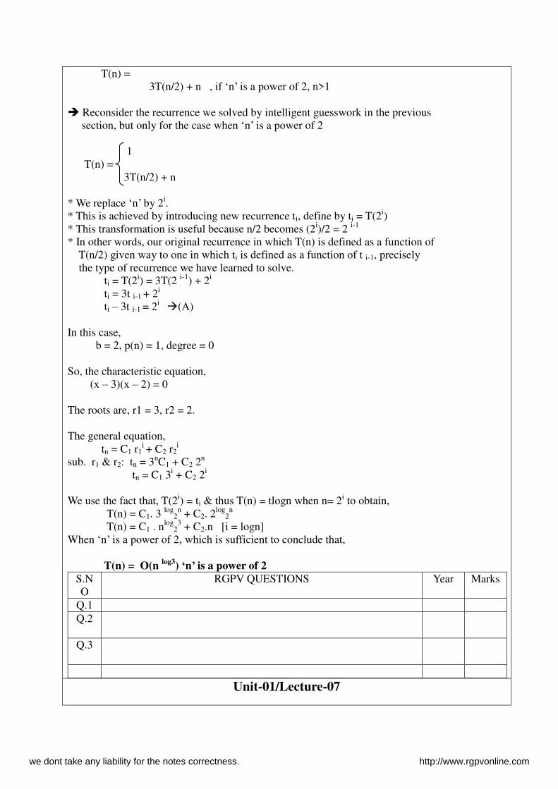
T(n) = 3T(n/2) + n , if ‘n’ is a power of 2, n>1 Reconsider the recurrence we solved by intelligent guesswork in the previous section, but only for the case when ‘n’ is a power of 2 1 T(n) = 3T(n/2) + n * We replace ‘n’ by 2i. * This is achieved by introducing new recurrence ti, define by ti = T(2i) * This transformation is useful because n/2 becomes (2i)/2 = 2 i-1 * In other words, our original recurrence in which T(n) is defined as a function of T(n/2) given way to one in which ti is defined as a function of t i-1, precisely the type of recurrence we have learned to solve. ti = T(2i) = 3T(2 i-1) + 2i ti = 3t i-1 + 2i ti – 3t i-1 = 2i (A) In this case, b = 2, p(n) = 1, degree = 0 So, the characteristic equation, (x – 3)(x – 2) = 0 The roots are, r1 = 3, r2 = 2. The general equation, tn = C1 r1

i + C2 r2i

sub. r1 & r2: tn = 3nC1 + C2 2n

tn = C1 3i + C2 2

i

We use the fact that, T(2i) = ti & thus T(n) = tlogn when n= 2i to obtain, T(n) = C1. 3 log

2n + C2. 2

log2

n T(n) = C1 . n

log2

3 + C2.n [i = logn] When ‘n’ is a power of 2, which is sufficient to conclude that, T(n) = O(n

log3) ‘n’ is a power of 2

S.NO


Q.1 Q.2

Q.3

Unit-01/Lecture-07


Binary search

Binary search:

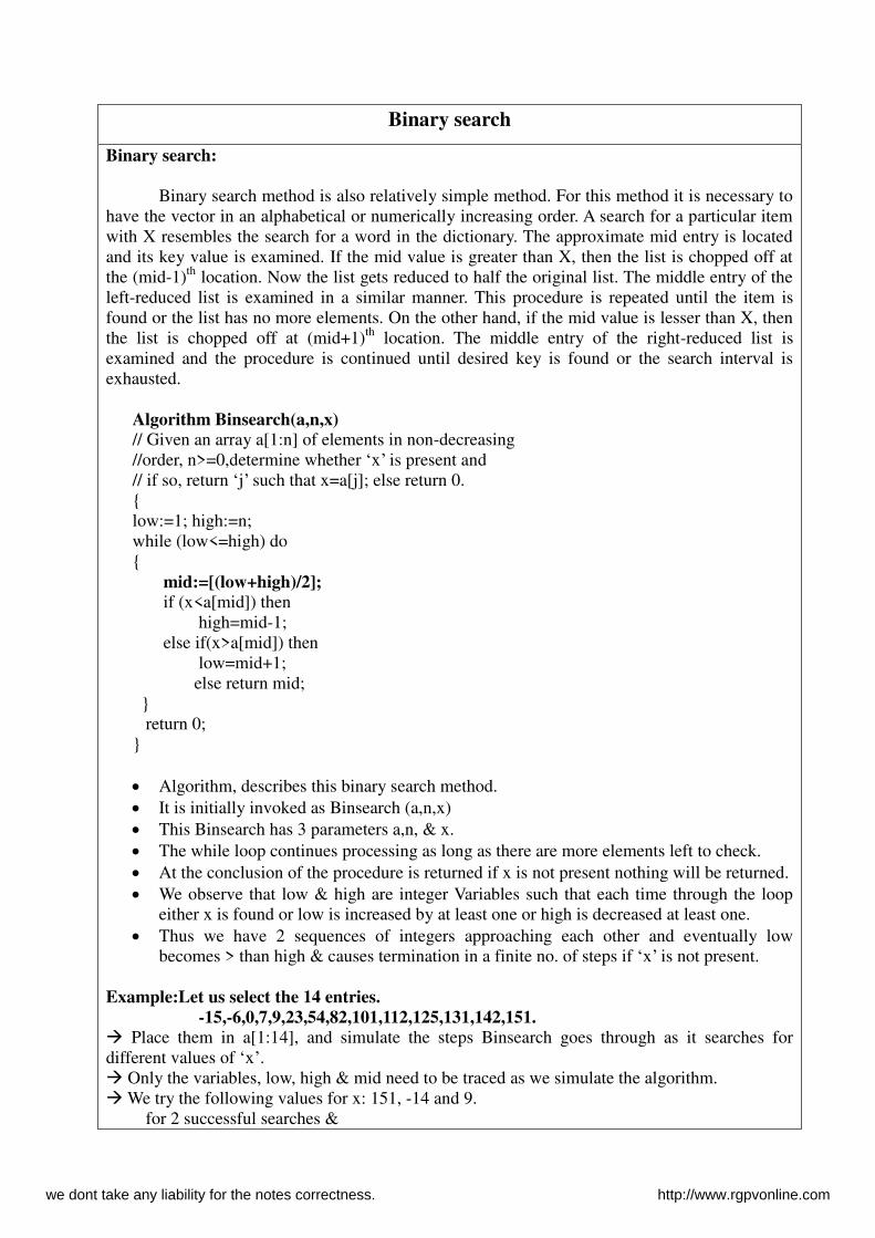
Binary search method is also relatively simple method. For this method it is necessary to have the vector in an alphabetical or numerically increasing order. A search for a particular item with X resembles the search for a word in the dictionary. The approximate mid entry is located and its key value is examined. If the mid value is greater than X, then the list is chopped off at the (mid-1)th location. Now the list gets reduced to half the original list. The middle entry of the left-reduced list is examined in a similar manner. This procedure is repeated until the item is found or the list has no more elements. On the other hand, if the mid value is lesser than X, then the list is chopped off at (mid+1)th location. The middle entry of the right-reduced list is examined and the procedure is continued until desired key is found or the search interval is exhausted.

Algorithm Binsearch(a,n,x)

// Given an array a[1:n] of elements in non-decreasing //order, n>=0,determine whether ‘x’ is present and // if so, return ‘j’ such that x=a[j]; else return 0. { low:=1; high:=n; while (low<=high) do { mid:=[(low+high)/2];

if (x<a[mid]) then high=mid-1; else if(x>a[mid]) then low=mid+1; else return mid; } return 0; } Algorithm, describes this binary search method. It is initially invoked as Binsearch (a,n,x) This Binsearch has 3 parameters a,n, & x. The while loop continues processing as long as there are more elements left to check. At the conclusion of the procedure is returned if x is not present nothing will be returned. We observe that low & high are integer Variables such that each time through the loop

either x is found or low is increased by at least one or high is decreased at least one. Thus we have 2 sequences of integers approaching each other and eventually low

becomes > than high & causes termination in a finite no. of steps if ‘x’ is not present. Example:Let us select the 14 entries.

-15,-6,0,7,9,23,54,82,101,112,125,131,142,151.

Place them in a[1:14], and simulate the steps Binsearch goes through as it searches for different values of ‘x’. Only the variables, low, high & mid need to be traced as we simulate the algorithm. We try the following values for x: 151, -14 and 9. for 2 successful searches &


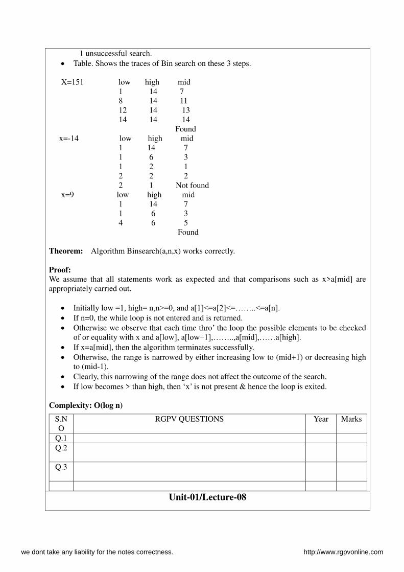
1 unsuccessful search. Table. Shows the traces of Bin search on these 3 steps. X=151 low high mid

1 14 7 8 14 11 12 14 13 14 14 14 Found x=-14 low high mid 1 14 7 1 6 3 1 2 1 2 2 2 2 1 Not found x=9 low high mid 1 14 7 1 6 3 4 6 5 Found

Theorem: Algorithm Binsearch(a,n,x) works correctly. Proof:

We assume that all statements work as expected and that comparisons such as x>a[mid] are appropriately carried out.

Initially low =1, high= n,n>=0, and a[1]<=a[2]<=……..<=a[n]. If n=0, the while loop is not entered and is returned. Otherwise we observe that each time thro’ the loop the possible elements to be checked

of or equality with x and a[low], a[low+1],……..,a[mid],……a[high]. If x=a[mid], then the algorithm terminates successfully. Otherwise, the range is narrowed by either increasing low to (mid+1) or decreasing high

to (mid-1). Clearly, this narrowing of the range does not affect the outcome of the search. If low becomes > than high, then ‘x’ is not present & hence the loop is exited.

Complexity: O(log n)

S.NO


Q.1 Q.2

Q.3

Unit-01/Lecture-08


Merge sort

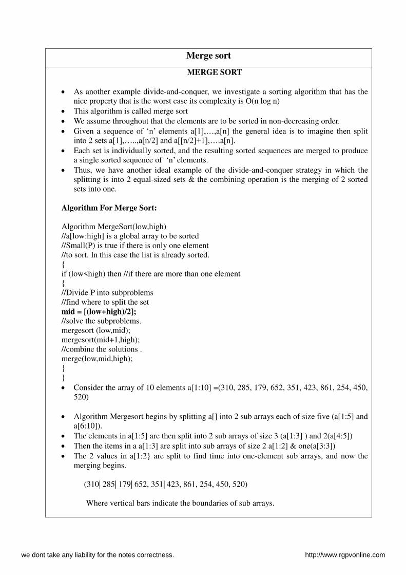
MERGE SORT

As another example divide-and-conquer, we investigate a sorting algorithm that has the nice property that is the worst case its complexity is O(n log n)

This algorithm is called merge sort We assume throughout that the elements are to be sorted in non-decreasing order. Given a sequence of ‘n’ elements a[1],…,a[n] the general idea is to imagine then split

into 2 sets a[1],…..,a[n/2] and a[[n/2]+1],….a[n]. Each set is individually sorted, and the resulting sorted sequences are merged to produce

a single sorted sequence of ‘n’ elements. Thus, we have another ideal example of the divide-and-conquer strategy in which the

splitting is into 2 equal-sized sets & the combining operation is the merging of 2 sorted sets into one.

Algorithm For Merge Sort:

Algorithm MergeSort(low,high) //a[low:high] is a global array to be sorted //Small(P) is true if there is only one element //to sort. In this case the list is already sorted. { if (low<high) then //if there are more than one element { //Divide P into subproblems //find where to split the set mid = [(low+high)/2];

//solve the subproblems. mergesort (low,mid); mergesort(mid+1,high); //combine the solutions . merge(low,mid,high); } } Consider the array of 10 elements a[1:10] =(310, 285, 179, 652, 351, 423, 861, 254, 450,

520) Algorithm Mergesort begins by splitting a[] into 2 sub arrays each of size five (a[1:5] and

a[6:10]). The elements in a[1:5] are then split into 2 sub arrays of size 3 (a[1:3] ) and 2(a[4:5]) Then the items in a a[1:3] are split into sub arrays of size 2 a[1:2] & one(a[3:3]) The 2 values in a[1:2} are split to find time into one-element sub arrays, and now the

merging begins.

(310| 285| 179| 652, 351| 423, 861, 254, 450, 520)

Where vertical bars indicate the boundaries of sub arrays.


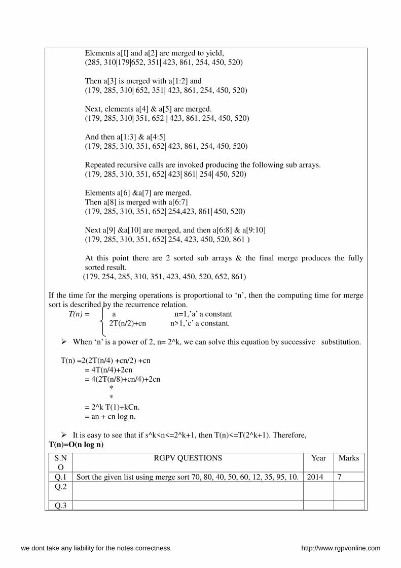
Elements a[I] and a[2] are merged to yield, (285, 310|179|652, 351| 423, 861, 254, 450, 520)

Then a[3] is merged with a[1:2] and (179, 285, 310| 652, 351| 423, 861, 254, 450, 520)

Next, elements a[4] & a[5] are merged. (179, 285, 310| 351, 652 | 423, 861, 254, 450, 520)

And then a[1:3] & a[4:5] (179, 285, 310, 351, 652| 423, 861, 254, 450, 520)

Repeated recursive calls are invoked producing the following sub arrays. (179, 285, 310, 351, 652| 423| 861| 254| 450, 520)

Elements a[6] &a[7] are merged. Then a[8] is merged with a[6:7] (179, 285, 310, 351, 652| 254,423, 861| 450, 520)

Next a[9] &a[10] are merged, and then a[6:8] & a[9:10] (179, 285, 310, 351, 652| 254, 423, 450, 520, 861 )

At this point there are 2 sorted sub arrays & the final merge produces the fully sorted result.

(179, 254, 285, 310, 351, 423, 450, 520, 652, 861) If the time for the merging operations is proportional to ‘n’, then the computing time for merge sort is described by the recurrence relation.

T(n) = a n=1,’a’ a constant 2T(n/2)+cn n>1,’c’ a constant.

When ‘n’ is a power of 2, n= 2^k, we can solve this equation by successive substitution.

T(n) =2(2T(n/4) +cn/2) +cn

= 4T(n/4)+2cn = 4(2T(n/8)+cn/4)+2cn

* *

= 2^k T(1)+kCn. = an + cn log n.

It is easy to see that if s^k<n<=2^k+1, then T(n)<=T(2^k+1). Therefore,

T(n)=O(n log n)

S.NO


Q.1 Sort the given list using merge sort 70, 80, 40, 50, 60, 12, 35, 95, 10. 2014 7 Q.2

Q.3


Unit-01/Lecture-09

Quick sort

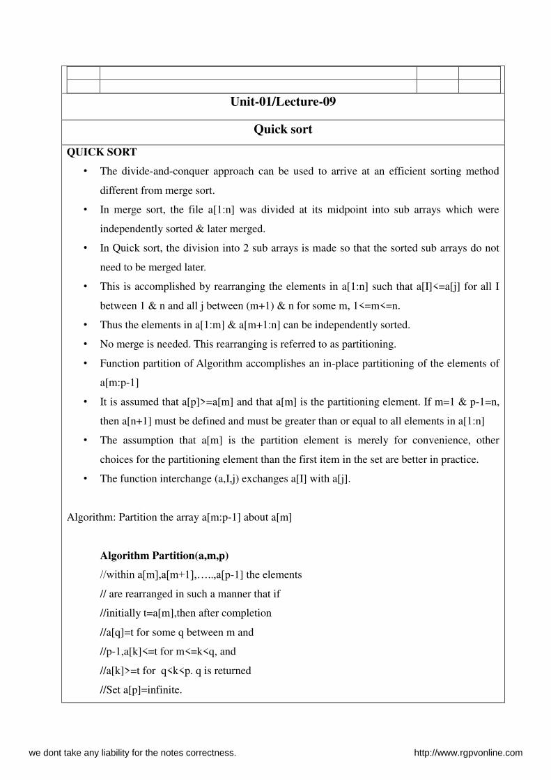
QUICK SORT

• The divide-and-conquer approach can be used to arrive at an efficient sorting method

different from merge sort.

• In merge sort, the file a[1:n] was divided at its midpoint into sub arrays which were

independently sorted & later merged.

• In Quick sort, the division into 2 sub arrays is made so that the sorted sub arrays do not

need to be merged later.

• This is accomplished by rearranging the elements in a[1:n] such that a[I]<=a[j] for all I

between 1 & n and all j between (m+1) & n for some m, 1<=m<=n.

• Thus the elements in a[1:m] & a[m+1:n] can be independently sorted.

• No merge is needed. This rearranging is referred to as partitioning.

• Function partition of Algorithm accomplishes an in-place partitioning of the elements of

a[m:p-1]

• It is assumed that a[p]>=a[m] and that a[m] is the partitioning element. If m=1 & p-1=n,

then a[n+1] must be defined and must be greater than or equal to all elements in a[1:n]

• The assumption that a[m] is the partition element is merely for convenience, other

choices for the partitioning element than the first item in the set are better in practice.

• The function interchange (a,I,j) exchanges a[I] with a[j].

Algorithm: Partition the array a[m:p-1] about a[m]

Algorithm Partition(a,m,p)

//within a[m],a[m+1],…..,a[p-1] the elements

// are rearranged in such a manner that if

//initially t=a[m],then after completion

//a[q]=t for some q between m and

//p-1,a[k]<=t for m<=k<q, and

//a[k]>=t for q<k<p. q is returned

//Set a[p]=infinite.


{

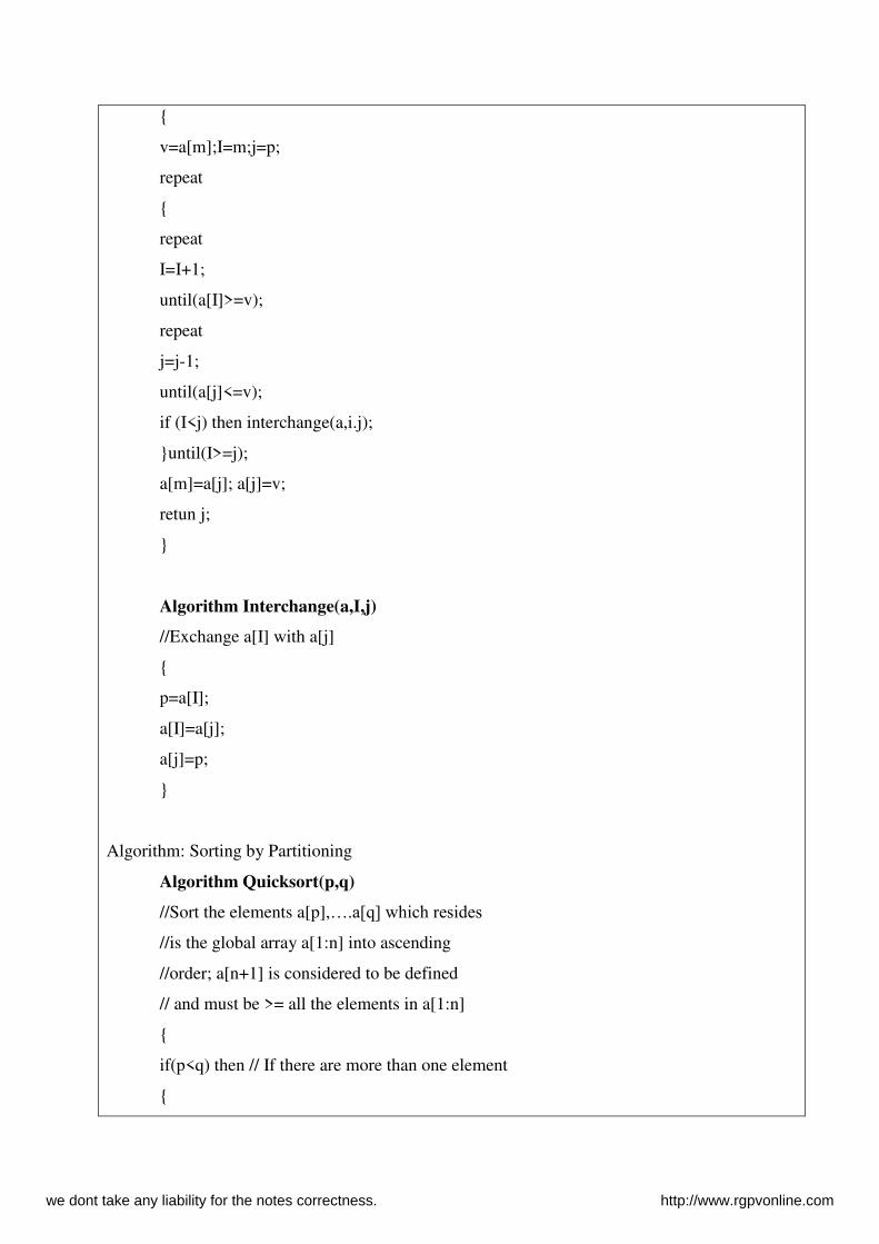
v=a[m];I=m;j=p;

repeat

{

repeat

I=I+1;

until(a[I]>=v);

repeat

j=j-1;

until(a[j]<=v);

if (I<j) then interchange(a,i.j);

}until(I>=j);

a[m]=a[j]; a[j]=v;

retun j;

}

Algorithm Interchange(a,I,j)

//Exchange a[I] with a[j]

{

p=a[I];

a[I]=a[j];

a[j]=p;

}

Algorithm: Sorting by Partitioning

Algorithm Quicksort(p,q)

//Sort the elements a[p],….a[q] which resides

//is the global array a[1:n] into ascending

//order; a[n+1] is considered to be defined

// and must be >= all the elements in a[1:n]

{

if(p<q) then // If there are more than one element

{


// divide p into 2 subproblems

j=partition(a,p,q+1);

//’j’ is the position of the partitioning element.

//solve the subproblems.

quicksort(p,j-1);

quicksort(j+1,q);

//There is no need for combining solution.

}

}

Complexity: O(n log n)- Best and Average case

O(n2) in worst case

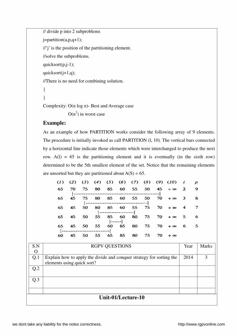
Example:

As an example of how PARTITION works consider the following array of 9 elements.

The procedure is initially invoked as call PARTITION (l, 10). The vertical bars connected

by a horizontal line indicate those elements which were interchanged to produce the next

row. A(l) = 65 is the partitioning element and it is eventually (in the sixth row)

determined to be the 5th smallest element of the set. Notice that the remaining elements

are unsorted but they are partitioned about A(S) = 65.

S.NO


Q.1 Explain how to apply the divide and conquer strategy for sorting the elements using quick sort?

2014 3

Q.2

Q.3

Unit-01/Lecture-10


Strassen’s matrix multiplication

STRASSON’S MATRIX MULTIPLICAION

Let A and B be the 2 n*n Matrix. The product matrix C=AB is calculated by using the formula, C (i ,j )= A(i,k) B(k,j) for all ‘i’ and and j between 1 and n.

The time complexity for the matrix Multiplication is O(n3). Divide and conquer method suggest another way to compute the product of n*n matrix. We assume that N is a power of 2 .In the case N is not a power of 2 ,then enough rows

and columns of zero can be added to both A and B .SO that the resulting dimension are the powers of two.

If n=2 then the following formula as a computed using a matrix multiplication operation for the elements of A & B.

If n>2,Then the elements are partitioned into sub matrix n/2*n/2..since ‘n’ is a power of 2 these product can be recursively computed using the same formula .This Algorithm will continue applying itself to smaller sub matrix until ‘N” become suitable small(n=2) so that the product is computed directly .

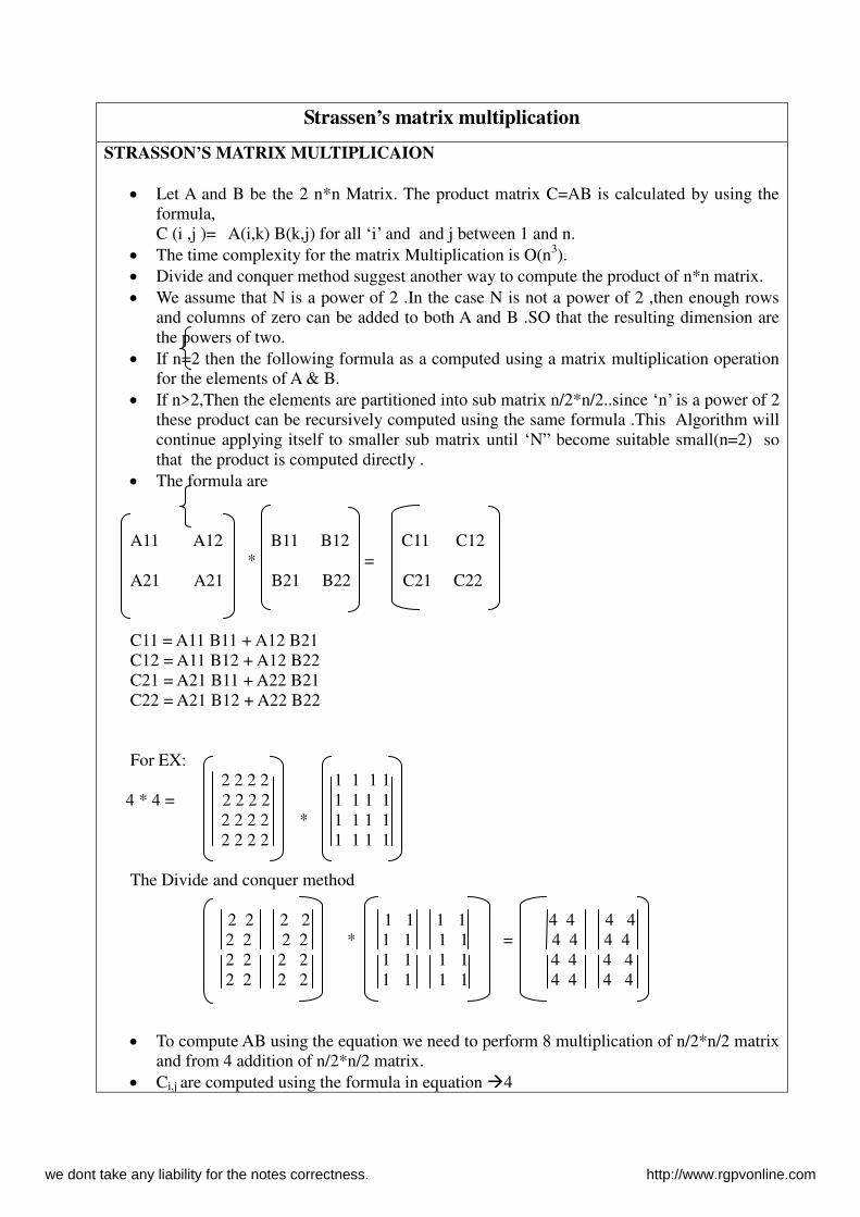
The formula are

A11 A12 B11 B12 C11 C12 * = A21 A21 B21 B22 C21 C22 C11 = A11 B11 + A12 B21 C12 = A11 B12 + A12 B22 C21 = A21 B11 + A22 B21 C22 = A21 B12 + A22 B22 For EX: 2 2 2 2 1 1 1 1

4 * 4 = 2 2 2 2 1 1 1 1 2 2 2 2 * 1 1 1 1 2 2 2 2 1 1 1 1

The Divide and conquer method 2 2 2 2 1 1 1 1 4 4 4 4 2 2 2 2 * 1 1 1 1 = 4 4 4 4 2 2 2 2 1 1 1 1 4 4 4 4 2 2 2 2 1 1 1 1 4 4 4 4 To compute AB using the equation we need to perform 8 multiplication of n/2*n/2 matrix

and from 4 addition of n/2*n/2 matrix. Ci,j are computed using the formula in equation 4


As can be sum P, Q, R, S, T, U, and V can be computed using 7 Matrix multiplication and 10 addition or subtraction.

The Cij are required addition 8 addition or subtraction. T(n)= b n<=2 a &b are 7T(n/2)+an2 n>2 constant Finally we get T(n) =O( nlog

27)

since n/2 * n/2 matrix can be can be added in Cn for some constant C, The overall computing time T(n) of the resulting divide and conquer algorithm is given by the sequence.

T(n)= b n<=2 a &b are 8T(n/2)+cn^2 n>2 constant

That is T(n)= O( nlog

28)=O(n3)

* Matrix multiplication are more expensive then the matrix addition O(n^3).We can attempt to reformulate the equation for Cij so as to have fewer multiplication and possibly more addition .

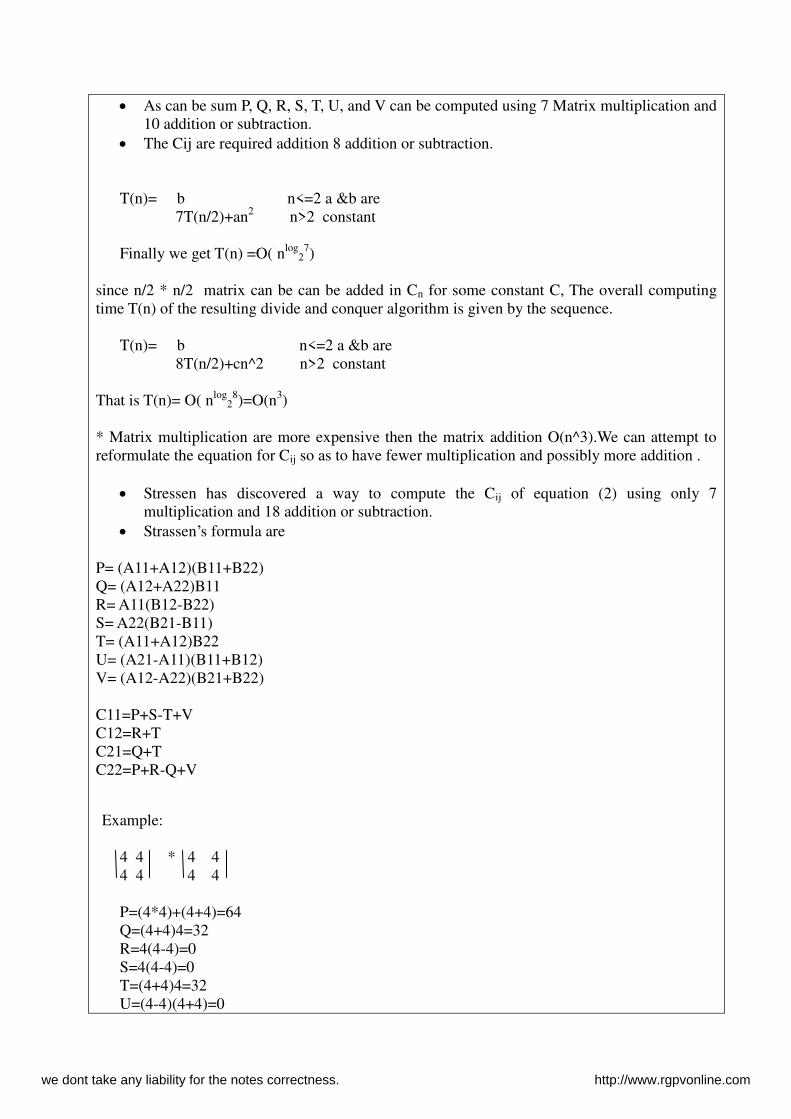
Stressen has discovered a way to compute the Cij of equation (2) using only 7 multiplication and 18 addition or subtraction.

Strassen’s formula are P= (A11+A12)(B11+B22) Q= (A12+A22)B11 R= A11(B12-B22) S= A22(B21-B11) T= (A11+A12)B22 U= (A21-A11)(B11+B12) V= (A12-A22)(B21+B22) C11=P+S-T+V C12=R+T C21=Q+T C22=P+R-Q+V

Example: 4 4 * 4 4

4 4 4 4 P=(4*4)+(4+4)=64 Q=(4+4)4=32 R=4(4-4)=0 S=4(4-4)=0 T=(4+4)4=32 U=(4-4)(4+4)=0


V=(4-4)(4+4)=0 C11=(64+0-32+0)=32 C12=0+32=32 C21=32+0=32 C22=64+0-32+0=32 So the answer c(i,j) is 32 32

32 32 S.NO


Q.1 Explain the Strassen’s multiplication technique? 2014 2 Q.2

Q.3


1 Unit-01/Lecture-01 Introduction to Algorithms, Designing ...

Documents