1-s2.0-S1476927115000547-main.pdf

Page 1

R

Og

CAa

b

c

d

e

f

g

h

a

ARRAA

KGDHQS

1

waiaatrmsao

M

d((

h1

Computational Biology and Chemistry 56 (2015) 98–108

Contents lists available at ScienceDirect

Computational Biology and Chemistry

journa l homepage: www.e lsev ier .com/ locate /compbio lchem

esearch Article

n the impact of discreteness and abstractions on modelling noise inene regulatory networks

hiara Bodeia, Luca Bortolussib,g,h, Davide Chiarugig,c,∗, Maria Luisa Guerrierod,lberto Policriti e, Alessandro Romanel f

Dip. di Informatica, Università di Pisa, ItalyDip. di Matematica e Geoscienze, Università di Trieste, ItalyMax Planck Institut of Colloids and Interfaces, Potsdam, GermanySystems Biology Ireland, University College Dublin, IrelandDip. di Matematica e Informatica, Università di Udine, Udine, ItalyCentre for Integrative Biology (CIBIO), University of Trento, ItalyCNR-ISTI, Pisa, ItalyModelling and Simulation Group, University of Saarland, Campus E 1 3, Saarbruecken, Germany

r t i c l e i n f o

rticle history:eceived 13 August 2014eceived in revised form 26 February 2015ccepted 7 April 2015vailable online 8 April 2015

a b s t r a c t

In this paper, we explore the impact of different forms of model abstraction and the role of discretenesson the dynamical behaviour of a simple model of gene regulation where a transcriptional repressor nega-tively regulates its own expression. We first investigate the relation between a minimal set of parametersand the system dynamics in a purely discrete stochastic framework, with the twofold purpose of provid-ing an intuitive explanation of the different behavioural patterns exhibited and of identifying the main

eywords:ene regulatory networksiscrete modellingybrid systemuasi-steady state approximation

sources of noise. Then, we explore the effect of combining hybrid approaches and quasi-steady stateapproximations on model behaviour (and simulation time), to understand to what extent dynamics andquantitative features such as noise intensity can be preserved.

© 2015 Elsevier Ltd. All rights reserved.

tochastic noise

. Introduction

Regulating gene expression is a complex work of orchestration,here the instruments play with improvised variations withoutfixed music sheet. Under this regard, the regulation process,

n which DNA drives the synthesis of cell products such as RNA,nd proteins, can be thought of as a stochastic process. Themount of RNA and proteins in living cells must be thoroughlyuned, both to manage effectively housekeeping functions and to

espond promptly to upcoming needs (e.g. to adapt to environ-ental changes). To this end, gene expression is equipped with

everal control mechanisms and strategies that grant both reli-bility and flexibility in terms of throughput. Nevertheless, whenbserved at the single cell level, the amount of molecules involved

∗ Corresponding author at: Max Planck Institute of Colloids and Interfaces, Amühlenberg 1, 14476 Potsdam, Germany. Tel.: +49 (331) 567 9617.

E-mail addresses: [email protected] (C. Bodei), [email protected] (L. Bortolussi),[email protected] (D. Chiarugi), [email protected]. Guerriero), [email protected] (A. Policriti), [email protected]. Romanel).

ttp://dx.doi.org/10.1016/j.compbiolchem.2015.04.004476-9271/© 2015 Elsevier Ltd. All rights reserved.

in gene expression and its regulation fluctuates randomly (Raj andvan Oudenaarden, 2009). This stochastic effect at the molecularlevel turns out to play important roles in conditioning cell-scalephenomena, e.g. cellular fate decision making, incomplete pene-trance or enhanced fitness through phenotypes variability (Raj andvan Oudenaarden, 2009).

Pioneering works (Novic and Weiner, 1957; Ross et al., 1994)showed that gene expression in populations of genotypically iden-tical cells (i.e. with the same genetic constitution) is highly variableeven when epigenetic conditions (i.e. the ones that result fromexternal rather than genetic influence) are kept constant. In Elowitzet al. (2002), the authors identified such a population variabilityand decomposed the extrinsic and intrinsic contributions therein.Also, in Murphy et al. (2010), it is shown that this variability it iscontrollable.

Recent developments in experimental techniques (see Raj andvan Oudenaarden (2009) for a review) have made it possible to

detect and count individual molecules and, therefore, to measurethe amount of mRNA and proteins in single cells. These measure-ments have clearly shown that the number of mRNA and proteinscan vary significantly from cell to cell. This variability is caused

Page 2

logy a

bii(m

aebbiett2o

gotAKrrwbubafpie

klbtrtt

ucaitflt(1

tEt(Hpicts

cac

C. Bodei et al. / Computational Bio

y the fundamentally stochastic nature of the biochemical eventsnvolved in gene expression (Raj and van Oudenaarden, 2009) ands studied, e.g., in Mantzaris (2007), Stamatakis and Zygourakis2010), Stamatakis and Zygourakis (2011), where population-level

athematical frameworks are introduced and applied.As a consequence, the phenotypical variability (i.e. the vari-

bility resulting from the interaction of the genotype with thenvironment) exhibited by populations of identical organisms cane directly caused by stochasticity at the single cell level. Thus, it isecoming clear that noise and stochasticity underlie critical events

n cell’s life such as differentiation and decision making (Balázsit al., 2011). Moreover, some authors suggest that random pheno-ypic switching can represent an efficient mechanism for adaptingo fluctuating environments (see, e.g., Balázsi et al., 2011; Raj et al.,010). These findings have raised new interest in analysing the rolef noise in gene expression.

The regulation process includes multiple steps leading fromene transcription to the translation of the resulting mRNA tobtain the encoded protein. Each step represents a possible con-rol point, where several biochemical mechanisms play a role (seelberts et al. (2002) for a comprehensive review and Lillacci andhammash (2010) for an application to model selection). Cha-acterising the contributions of each single control point in theegulation process of gene expression is a complex task. Identifyinghich strategies come into play in generating or dampening noisy

ehaviours is even more challenging. The extensively studied reg-lation paradigm represented by the feedback control strategy cane used to explain the mechanisms controlling gene transcriptionnd translation. In such mechanisms, the global intensity of theeedback depends on parameters related to every single controloint. Computational methods can significantly help investigat-

ng the synergistic mechanisms underlying the regulation of genexpression.

There are several modelling strategies that can lead to differentinds of computational models, depending on both the particu-ar purposes and on the features of the available data. Models ofiological systems proposed in the literature can vary in terms ofhe abstraction level used to represent molecular amounts (in thisegard a model can be either discrete or continuous) and in terms ofhe underlying paradigm used for describing the temporal evolu-ion of the system, which can be either deterministic or stochastic.

Ordinary Differential Equations (ODEs) have been extensivelysed over the years to describe the behaviour of biological pro-esses. They provide modellers with powerful and well assessednalysis and simulation techniques. Nevertheless, ODE modelsmplicitly assume continuous and deterministic change of concen-rations, abstracting away noise and randomness due to stochasticuctuations. This, for example, makes it difficult to capture quali-atively different outcomes arising from identical initial conditionse.g., Raj and van Oudenaarden, 2008; Hume, 2000; Ross et al.,994).

One way to represent noise is to couple a Gaussian noise termo the model equations, obtaining a set of Stochastic Differentialquations (SDEs). This approach succeeded in gaining insights onhe stochasticity of gene expression underlying circadian clocksChabot et al., 2007) and genetic switches (Becksei et al., 2001).owever, continuous methods still fail to properly describe varioushenomena arising from stochastic fluctuations in systems involv-

ng small copy numbers of molecules (Resat et al., 2009), as in thease of bimodal mRNA distributions generated by long transcrip-ional bursts, during which mRNA level approaches a new steadytate (Raj and van Oudenaarden, 2009).

The copy numbers of molecules and individual entities in theell space are discrete and the reactions in which they are involvedre stochastic events. Consequently, approaches based on a dis-rete and stochastic formulation, such as the ones built upon

nd Chemistry 56 (2015) 98–108 99

Continuous-Time Markov Chains (CTMCs) (McQuarrie, 1967;Bartholomay, 1958), have been successfully introduced to over-come the modelling limitations of continuous methods. Stochasticsystems are formally represented through a chemical master equa-tion and have also been studied, rather directly, in the form ofautocatalytic reactions systems, with approaches such as the onedescribed in Dauxois et al. (2009).

However, since the analytic solution of the underlying equationis often infeasible for real size systems, these models are usu-ally studied resorting to simulation approaches, mostly based on(variants of) Gillespie’s stochastic simulation algorithm (Gillespie,1977). Unfortunately, in some cases, even numerical simulationcan be computationally very expensive. A compromise betweenaccuracy and efficiency can be obtained by combining discreteand continuous evolution in so-called hybrid approaches (Pahle,2009; Bortolussi and Policriti, 2009, 2013). In this context, we recallalso (Salis and Kaznessis, 2005; Salis et al., 2006), where hybridapproaches for stochastic simulation of gene networks have beendeveloped.

In this work, we consider a simple model of gene regulation in atranscription/translation genetic network, where a transcriptionalrepressor negatively regulates its own expression. This modelhas been widely studied (e.g. Marquez Lago and Stelling, 2010;Stekel and Jenkins, 2008), because it is a minimal system thatexplicitly describes the processes of transcription and translationand because it is a basic component of many complex biolog-ical systems. Despite its apparent simplicity, understanding itsbehaviour is not easy, because this is governed in a non-trivial wayby several quantitative parameters. Actually, different parametercombinations lead to a range of qualitatively different dynamics.In particular, in Marquez Lago and Stelling (2010), the intensity ofnoise in this system is analysed in terms of various parameters, withspecial emphasis on the strength of the negative feedback. Thatpaper demonstrates how the application of engineering principlesto the role of feedbacks in a biological context could be mislead-ing. The authors show, indeed, that noise generally increases withfeedback strength, in contrast to the common knowledge. Theyalso relate the possible different dynamical regimes with the differ-ent regions of the parameter space. The overall behaviour emergesfrom the complex interaction between feedback strength and otherparameters of the system, governing the dynamics of the proteinand of the mRNA.

Starting from the analysis proposed in Marquez Lago andStelling (2010), we investigate the model with two goals in mind:(i) identifying the parameters that play a key role in the regulationprocess, by systematically studying the impact of parameters varia-tions on the global dynamics of the system. In this way, we establisha link between the parameter space and the observed temporalpatterns, i.e. the diverse behavioural phenotypes; (ii) quantifyingthe impact of each reaction of the modelled system on the over-all dynamics and on noise patterns. This allows us to identify thosereactions that, having a minor influence on the global noise pattern,can be safely approximated in a deterministic fashion.

At a higher level and on a longer term, we aim at setting upa systematic strategy for correctly building hybrid models of bio-chemical systems. In such models, only the most relevant sources ofnoise will be represented via a fully detailed stochastic description.

The handy dimension of our model of gene regulation allowsus to play with different models and techniques. On the one hand,we study a stochastic model of the negative feedback loop to con-struct an exact picture of its possible behavioural patterns and ofthe effects of noise. This precision comes with a high computational

cost, especially for certain parameter sets. On the other hand, wesystematically apply various forms of model abstraction, in orderto mitigate the inefficiency of exact stochastic simulation meth-ods. In particular, we abstract the discrete stochastic dynamics into

Page 3

1 logy and Chemistry 56 (2015) 98–108

cnsn(

sh

asof

2

Lns

ttlaickufa

ntfteasmt

obppetn

pfcp

TBf

Table 2Summary of the combinations of parameters considered and their respective initialvalues for XP and XM .

˛

0.0166 16.6 16600

ˇ100 L-H M-H H-H1 L-M M-M H-M0.01 L-L M-L H-L

00 C. Bodei et al. / Computational Bio

ontinuous deterministic dynamics for some of the model compo-ents, thus obtaining a stochastic hybrid model. Afterwards, weimplify the model structure reducing the number of model compo-ents and reactions, by applying quasi-steady state approximationsQSSAs).

These abstractions are not blindly applied, but are rather con-idered only in the regions of the parameter space for which theypotheses underlying these techniques are (reasonably) satisfied.

We believe that the methodology we adopt is a reliablepproach for modelling in systems biology, where too often inilico techniques based on abstractions or approximations are usedff-the-shelf, without any concern on their applicability and faith-ulness.

. The model

The model we consider, described among others in Marquezago and Stelling (2010), Stekel and Jenkins (2008), is a geneticetwork composed by the reactions reported in Table 1 andchematically represented in Fig. 1(a).

The model is a minimal system that describes the self-regulatedranscription/translation of a gene into a protein. The gene (G) isranscribed into an mRNA molecule (M), which in turn is trans-ated into a protein P. P regulates its own expression by means of

negative feedback loop: P can bind to G, making it switch fromts free active state to an inactive state (Gb). Finally, both M and Pan be degraded. All reactions are assumed to follow mass actioninetics, i.e. the speed of the reaction is proportional to the prod-ct of the amounts of each reactant and a kinetic constant. In theollowing, the amounts of P, M, G, and Gb are denoted by XP, XM, XG,nd XGb, respectively.

Similarly to Marquez Lago and Stelling (2010), we ignore copy-umber variations (CNVs) and assume to have a single copy ofhe gene. The reason for this assumption is that CNVs may riserom different structural rearrangements (e.g. deletions, duplica-ions, inversions) and can involve different genomic regions (e.g.nhancer, promoter, coding), hence having potentially differentnd sometimes unpredictable effects on the expression of theurrounding/overlapping genes. These effects may be difficult toodel and may introduce a level of variability that goes beyond

he aim of this work.In Marquez Lago and Stelling (2010), a very detailed phenomen-

logical description of the different behaviours of the model haseen carried out, changing parameters in order to explore a largeortion of the parameters’ space. The authors claim that this sim-le feedback network has a counter-intuitive behaviour: while, inngineering, negative feedbacks are assumed to be a mechanismo decrease noise, the authors show that in this network, instead,oise increases with feedback strength.

Following on from those results, in this section we provide a sim-ler picture of the possible behavioural patterns of the model; we

ound out, in fact, that the seemingly counter-intuitive behaviouran be explained by analysing a combination of a minimal set ofarameters.

able 1iochemical reactions of the self-repressing gene network considered. All reactions

ollow mass action kinetics and the units of their rate constants are s−1.

Rate constant Reaction Description

prod M G → G + M mRNA production (transcription)prod P M → M + P protein production (translation)deg M M →∅ mRNA degradationdeg P P →∅ protein degradationbind P G + P → Gb repressor bindingunbind P Gb → G + P repressor unbinding

XP0 86000 2700 86XM0 25 1 0

First of all, with a preliminary high level analysis of the stochasticdynamics of M, P, gene repression, and of the interactions betweendynamical regimes involved in the model (partly reported in theSupplementary Material, Appendix A), we identified the followingtwo key parameters:

(1) P binding/unbinding ratio ˛ = bindP/unbindP;(2) P/M degradation ratio ˇ = degP/degM.

The first parameter ˛ was used in Marquez Lago and Stelling(2010) as an indicator of the strength of the feedback regulation: thehigher the value of ˛, the stronger the repression and the smallerthe number of mRNA molecules on average. While in MarquezLago and Stelling (2010) the authors fix the binding rate and varythe unbinding rate (thus increasing feedback strength by increas-ing the binding strength), in our work we fix the unbinding rateand vary the binding rate (thus increasing feedback strength byincreasing the binding affinity), hence using a different mecha-nism to represent repression intensity. This choice has an impacton the dynamics of the network, in particular on the behaviour ofthe bursty protein regime and on the feasibility of the QSSA (seealso Section 3.3 and Appendix A in the Supplementary Material).

The second parameter ˇ is the ratio between the half-life of M andthe half-life of P. From a dynamical point of view, it describes thespeed at which production and degradation of the protein reachequilibrium, relative to the mRNA. Essentially, it captures how theprotein level reacts to fluctuations at the mRNA level: the higherthe value of ˇ, the faster P’s response. This means that XM and XP

will be highly correlated for high ˇ, and so noise at the level of XM

level will propagate more effectively to XP.The values of the stochastic rate constants we use are based

on those from Marquez Lago and Stelling (2010) and their unitsare s−1. After a prescreening in which we used several valuesaccording to Marquez Lago and Stelling (2010) for stochastic simu-lations, we identified the values that proved to be representative inreproducing the complete gamut of all the interesting observablephenotypes. Therefore, in this work we choose to vary ˛ in the set{0.0166, 16.6, 16600}, and ˇ in the set {0.01, 1, 100}. In the follow-ing, we refer to these three values for ˛ and ˇ as low (L), medium(M), and high (H), and we refer to the combinations of parameterswith the names listed in Table 2.

The parameter ˛ is varied by fixing the value for unbindP to 1 andmodifying bindP, defined as ˛ · unbindP. Similarly, we fixed the valuefor degM to 0.001 and vary degP = ˇ · degM while varying ˇ. Moreover,we define P production rate as the product of P degradation rate andthe steady state value for P per M molecules, i.e. prodP = degP · Psteadywith Psteady equal to 3500. We have chosen this value because itallows us to obtain biologically meaningful numbers of proteinsfor all the parameter combinations. However, reasonably chang-ing this parameter does not disrupt the observed behaviours. This

enables us to explore parameter combinations with a low degrada-tion rate, ensuring that translation rate does not become too largeconsidering a maximum rate constant of 108–1010 M−1 s−1 (Zhouand Zhong, 1982) (see Appendix B in the Supplementary Material

Page 4

C. Bodei et al. / Computational Biology and Chemistry 56 (2015) 98–108 101

F ection and of its variants with QSSAs described in Section 4. Arrows indicate the directiono s which are on both the left- and the right-hand side of the reaction) with, respectively,p

fa1ai

2

so2t

pvesw

amfr

rotXi

tsdw

utacaMaoP

Table 3Statistics for different abstractions of the explicit stochastic model, computed from1000 simulated trajectories, sampled at time t = 10000 (see footnote 1).

˛-ˇ mean(XP) CV(XP) mean(XM) CV(XM) cor(XP ,XM)

Stochastic model with explicit binding and unbindingL-L 85986.95 0.008 24.47 0.2037 0.196L-M 86693.14 0.1027 24.908 0.1807 0.5633L-H 85662.71 0.1527 24.49 0.1527 0.9926M-L 2707.262 0.0425 0.788 0.8865 0.2433M-M 3231.701 0.5176 0.936 0.8501 0.5904M-H 4440.153 0.4492 1.27 0.4492 0.9803H-L 84.058 0.2310 0.027 6.0061 0.2160H-M 441.398 1.7066 0.165 2.2507 0.6555H-H 2176.477 0.7728 0.622 0.7833 0.9824

Hybrid model with explicit binding and unbindingL-L 85857.524 0.0077 24.752 0.1970 0.2052L-M 86285.457 0.1048 24.667 0.1839 0.5815L-H 86956.046 0.1467 24.881 0.1479 0.9910M-L 2724.2987 0.0426 0.797 1.1114 0.2315M-M 3313.9473 0.5245 0.962 0.8841 0.5635M-H 4454.3658 0.4429 1.274 0.4504 0.9803H-L 84.8464 0.246 0.024 6.3802 0.2677H-M 433.6356 1.7359 0.128 2.6114 0.649H-H 2201.9696 0.7615 0.628 0.7733 0.9897

Stochastic model with QSSA on binding/unbindingL-L 85978.76 0.0079 25.539 0.2034 0.2178L-M 85991.76 0.102 24.688 0.1759 0.5939L-H 88768.61 0.14 25.37 0.1400 0.9847M-L 2705.874 0.0429 0.751 1.1683 0.2280M-M 3259.29 0.5105 0.921 0.9133 0.6054M-H 4369.297 0.4506 1.249 0.4538 0.9828H-L 85.423 0.2427 0.026 6.1236 0.1210H-M 576.304 1.9408 0.21 2.753 0.6294H-H 3386.57 0.3392 0.967 0.3553 0.9569

Hybrid model with QSSA on binding/unbindingL-L 85832.168 0.0077 24.457 0.2001 0.2124

ig. 1. Diagrammatic representation of the gene regulatory model described in this sf reactions; dot-headed and T-headed lines represent reaction catalysts (i.e. specieositive and negative roles.

or further details). We finally fix prodM to 35 considering an aver-ge RNA polymerase transcription rate of 24–79 nucleotides/s and100 base pairs as the average size of an mRNA molecule (Vogelnd Jensen, 1994), i.e. an mRNA molecule is produced (on average)n 14–46 s.

.1. Analysis of stochastic behaviour

We proceed now by building a fully stochastic model from ouret of reactions, in order to undertake a thorough stochastic analysisf its dynamics. The simulation tool we use is COPASI (Hoops et al.,006), a framework that provides us with all the algorithms neededo run stochastic, hybrid, and deterministic simulations.

In order to outline the possible dynamics, we partition ourarameter space into different regions, by creating nine differentersions of our model, one for each parameter combination. Forach model we then set the initial amounts of M and P to the corre-ponding steady state values and run 1000 stochastic simulationsith limit time 10,000 s.1

As listed in Table 2, for combinations having low ˛, the initial XP

nd XM are 86, 000 and 25, respectively. For combinations havingedium ˛, the initial XP and XM are 2700 and 1, respectively. Finally,

or combinations having high ˛, the initial XP and XM are 86 and 0,espectively.

Fig. 2 shows, for each of the nine versions of the model, one rep-esentative simulated trajectory of XP together with its coefficientf variation (CV) and the correlation between XP and XM at time= 10, 000. A comprehensive summary of population statistics ofP and XM is reported in Table 3 (top panel), and further details are

n the Supplementary Material.With L-L combination we have that, since repression is weak,

he average XM value is relatively high and, consequently, XP steadytate is also high. Moreover, since P degradation is slower than Megradation, XP dynamics are slower than XM’s, i.e. XP fluctuatesith a lower frequency than XM does; moreover, at steady state XP

1 We empirically identified 10,000 s as a limit time that is long enough to allows to observe the specific steady state dynamics of P and M in all the parame-ers combinations we considered. Moreover, we are taking the population averaget the chosen time 10,000, and not the time average along a single trajectory, asommonly done. However, in our context, these two approaches are equivalent asll the models we consider are ergodic. This is obvious for the Continuous-Timearkov Chain (CTMC) models, but it can be shown also for the hybrid models, by

pplying a result in (Costa and Dufour, 2008), characterising ergodicity in termsf a Discrete-Time Markov Chain (DTMC) obtained by sampling trajectories of theiecewise Deterministic Markov Process (PDMP) at random times.

L-M 86562.663 0.105 24.608 0.1784 0.5904L-H 85935.261 0.1397 24.55 0.141 0.99M-L 2727.1072 0.04431 0.799 1.1134 0.2287M-M 3266.9487 0.5245 0.894 0.9301 0.5913M-H 4503.4732 0.445 1.289 0.4482 0.9766H-L 84.8650 0.2343 0.019 7.1891 0.1727

H-M 526.3546 1.8783 0.199 2.5999 0.6442H-H 3407.6452 0.3234 0.972 0.3370 0.9689

behaves like a simple birth-death process with very low noise. Wecan say that XP is very close to its deterministic average behaviour.

It is not surprising that this is also the combination with the low-est XP − XM correlation and coefficient of variation for XP. In case ofM-L combination P dynamics are still slower than M’s but repres-sion is stronger than before, causing XM and XP steady state values

Page 5

102 C. Bodei et al. / Computational Biology and Chemistry 56 (2015) 98–108

Fig. 2. Sampled XP trajectories from the explicit stochastic model computed using the Gibson-Bruck stochastic simulation algorithm (Gibson and Bruck, 2000) using differentc dicatd d at tit ice of

twsssbtsMi0bs

tetXtntaisiitPvlpi

h

ombinations of ˛ and ˇ values. The coefficient of variation and correlation trends inescribed in Section 3, and are computed from 1000 simulated trajectories, sampleime (t = 50, 000 s) to better visualise the long term trends and to show that the cho

o be much lower. In particular, XM starts to take very low valuesith fluctuations between 0 and 4 (see Fig. S1 for instances of XM

imulated trajectories). This combination of discreteness and pos-ible absence of M is immediately reflected in P dynamics. Indeed,uch dynamics are still very close to a simple birth-death processut, as indicated also by the increment of the coefficients of varia-ion for XM and XP, with higher noise. Combination H-L generates atrong gene repression that causes XM to fluctuate between 0 and 1.oreover, since P degradation is very low, the effect of repression

s even amplified by the almost constant presence of P, hence XM ismost of the time. As a consequence, XP tends to slowly degrade

ut displays some small “steps” corresponding to those rare andhort intervals in which XM takes value 1.

By increasing ˇ to a medium value, we have that XM and XP starto show a correlation higher than 0.5. In this parameter regions,ach change in XM is followed by a change in XP, that is quanti-atively equivalent (when scaled on XM). With L-M combinationM fluctuates at steady state around a value of 25, but in this casehe coefficient of variation is higher, meaning that its dynamics areoisier. Since the number of P molecules varies in accordance withhe number of M ones, we have that the noise in XM is reflected andmplified at the level of XP, generating a behaviour that is nois-er than in L-L. With M-M combination we can observe that XP

tarts to present an irregular fluctuating-like behaviour till reach-ng, with combination H-M, a behaviour that exhibits bursts. Thiss evidently caused by the high degree of discreteness in XM (i.e. XM

akes very small values). In particular, bursts are emerging becausedegradation is fast enough to increase the frequency of the inter-als in which XM is equal to 1 and to allow XP to rapidly reach aow amount when XM is back to 0. Note that the system alternates

eriods in which P is degraded to periods in which M is produced

n few copies, and so XP increases.When ˇ is high, P fluctuates with a higher frequency than M,

ence it reaches stochastic equilibrium faster than M. This causes,

ed by the arrows and in the panels are reported in detail on the top panel of Table 3,me t = 10, 000 s (see footnote 1). Note that the trajectories are reported for a longertime t = 10, 000 for computing the statistics is valid.

for all three values of ˛, the correlation between XP and XM to bevery high (greater than 0.98). With combination L-H XP fluctuatesaround the mean value with high level of noise. This increase innoise in all combinations having low ˛ can be visually observedalso in the XP distributions in Fig. S2. With the intermediate com-bination M-H, the time course of P copy number starts to exhibit amulti-modal behaviour. This can be explained by observing that XM

fluctuates between 0 and 3 and considering that, for a high value ofˇ, XP is able to reach its steady state between successive changes inXM level. Hence, P dynamics look like M’s with discrete levels prop-erly rescaled. From Fig. S2 it is easy to see that we have three maindiscrete levels of XP situated around 0, 3500, 7000 and 10, 500. Byfurther increasing the repression with H-H combination, we endup with a bimodal behaviour. This is clearly the consequence of thefact that, for high values of ˛, XM fluctuates only between 0 and 1,a behaviour that is shown by XP, which mainly alternates betweentwo discrete levels. From Fig. S2 we can observe that these twolevels are 0 and 3500.

Our exploration of the parameter space is clearly model-specificand cannot be directly generalised to other models of gene regu-latory networks; however, from a methodological point of view,our results clearly illustrate that this kind of thorough explorationis essential when studying genetic networks, in order to under-stand the role of feedback loops in generating different patterns oftime courses of both mRNA and translated proteins. In particular,we showed that certain parameter combinations are responsiblefor bursty temporal patterns. While there is strong experimen-tal evidence supporting transcriptional bursts both in prokaryotes(Golding et al., 2005) and (especially) in eukaryotes (Raj et al.,2006), the underlying biological mechanism still remains unclear.

Even though many complex mechanisms, involving the biochemi-cal machinery of DNA transcription, seem to contribute to pulsatiletranscription (as suggested in Golding et al. (2005)), our study sup-ports the fact that gene regulation mechanisms themselves (and the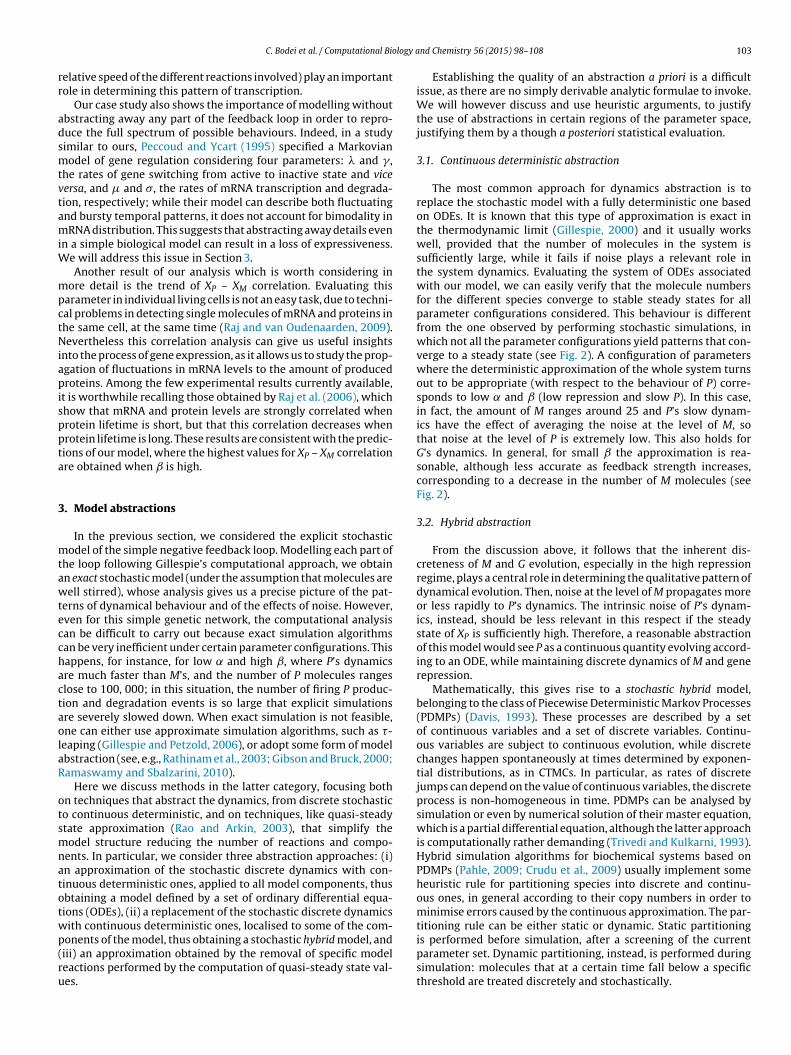

Page 6

logy a

rr

adsmtvtamiW

mpctNiapisppta

3

mtawtecchactaolaR

otsmnatotwp(ru

C. Bodei et al. / Computational Bio

elative speed of the different reactions involved) play an importantole in determining this pattern of transcription.

Our case study also shows the importance of modelling withoutbstracting away any part of the feedback loop in order to repro-uce the full spectrum of possible behaviours. Indeed, in a studyimilar to ours, Peccoud and Ycart (1995) specified a Markovianodel of gene regulation considering four parameters: � and � ,

he rates of gene switching from active to inactive state and viceersa, and � and �, the rates of mRNA transcription and degrada-ion, respectively; while their model can describe both fluctuatingnd bursty temporal patterns, it does not account for bimodality inRNA distribution. This suggests that abstracting away details even

n a simple biological model can result in a loss of expressiveness.e will address this issue in Section 3.Another result of our analysis which is worth considering in

ore detail is the trend of XP – XM correlation. Evaluating thisarameter in individual living cells is not an easy task, due to techni-al problems in detecting single molecules of mRNA and proteins inhe same cell, at the same time (Raj and van Oudenaarden, 2009).evertheless this correlation analysis can give us useful insights

nto the process of gene expression, as it allows us to study the prop-gation of fluctuations in mRNA levels to the amount of producedroteins. Among the few experimental results currently available,

t is worthwhile recalling those obtained by Raj et al. (2006), whichhow that mRNA and protein levels are strongly correlated whenrotein lifetime is short, but that this correlation decreases whenrotein lifetime is long. These results are consistent with the predic-ions of our model, where the highest values for XP – XM correlationre obtained when ˇ is high.

. Model abstractions

In the previous section, we considered the explicit stochasticodel of the simple negative feedback loop. Modelling each part of

he loop following Gillespie’s computational approach, we obtainn exact stochastic model (under the assumption that molecules areell stirred), whose analysis gives us a precise picture of the pat-

erns of dynamical behaviour and of the effects of noise. However,ven for this simple genetic network, the computational analysisan be difficult to carry out because exact simulation algorithmsan be very inefficient under certain parameter configurations. Thisappens, for instance, for low ˛ and high ˇ, where P’s dynamicsre much faster than M’s, and the number of P molecules rangeslose to 100, 000; in this situation, the number of firing P produc-ion and degradation events is so large that explicit simulationsre severely slowed down. When exact simulation is not feasible,ne can either use approximate simulation algorithms, such as �-eaping (Gillespie and Petzold, 2006), or adopt some form of modelbstraction (see, e.g., Rathinam et al., 2003; Gibson and Bruck, 2000;amaswamy and Sbalzarini, 2010).

Here we discuss methods in the latter category, focusing bothn techniques that abstract the dynamics, from discrete stochastico continuous deterministic, and on techniques, like quasi-steadytate approximation (Rao and Arkin, 2003), that simplify theodel structure reducing the number of reactions and compo-

ents. In particular, we consider three abstraction approaches: (i)n approximation of the stochastic discrete dynamics with con-inuous deterministic ones, applied to all model components, thusbtaining a model defined by a set of ordinary differential equa-ions (ODEs), (ii) a replacement of the stochastic discrete dynamicsith continuous deterministic ones, localised to some of the com-

onents of the model, thus obtaining a stochastic hybrid model, andiii) an approximation obtained by the removal of specific modeleactions performed by the computation of quasi-steady state val-es.

nd Chemistry 56 (2015) 98–108 103

Establishing the quality of an abstraction a priori is a difficultissue, as there are no simply derivable analytic formulae to invoke.We will however discuss and use heuristic arguments, to justifythe use of abstractions in certain regions of the parameter space,justifying them by a though a posteriori statistical evaluation.

3.1. Continuous deterministic abstraction

The most common approach for dynamics abstraction is toreplace the stochastic model with a fully deterministic one basedon ODEs. It is known that this type of approximation is exact inthe thermodynamic limit (Gillespie, 2000) and it usually workswell, provided that the number of molecules in the system issufficiently large, while it fails if noise plays a relevant role inthe system dynamics. Evaluating the system of ODEs associatedwith our model, we can easily verify that the molecule numbersfor the different species converge to stable steady states for allparameter configurations considered. This behaviour is differentfrom the one observed by performing stochastic simulations, inwhich not all the parameter configurations yield patterns that con-verge to a steady state (see Fig. 2). A configuration of parameterswhere the deterministic approximation of the whole system turnsout to be appropriate (with respect to the behaviour of P) corre-sponds to low ˛ and ˇ (low repression and slow P). In this case,in fact, the amount of M ranges around 25 and P’s slow dynam-ics have the effect of averaging the noise at the level of M, sothat noise at the level of P is extremely low. This also holds forG’s dynamics. In general, for small ˇ the approximation is rea-sonable, although less accurate as feedback strength increases,corresponding to a decrease in the number of M molecules (seeFig. 2).

3.2. Hybrid abstraction

From the discussion above, it follows that the inherent dis-creteness of M and G evolution, especially in the high repressionregime, plays a central role in determining the qualitative pattern ofdynamical evolution. Then, noise at the level of M propagates moreor less rapidly to P’s dynamics. The intrinsic noise of P’s dynam-ics, instead, should be less relevant in this respect if the steadystate of XP is sufficiently high. Therefore, a reasonable abstractionof this model would see P as a continuous quantity evolving accord-ing to an ODE, while maintaining discrete dynamics of M and generepression.

Mathematically, this gives rise to a stochastic hybrid model,belonging to the class of Piecewise Deterministic Markov Processes(PDMPs) (Davis, 1993). These processes are described by a setof continuous variables and a set of discrete variables. Continu-ous variables are subject to continuous evolution, while discretechanges happen spontaneously at times determined by exponen-tial distributions, as in CTMCs. In particular, as rates of discretejumps can depend on the value of continuous variables, the discreteprocess is non-homogeneous in time. PDMPs can be analysed bysimulation or even by numerical solution of their master equation,which is a partial differential equation, although the latter approachis computationally rather demanding (Trivedi and Kulkarni, 1993).Hybrid simulation algorithms for biochemical systems based onPDMPs (Pahle, 2009; Crudu et al., 2009) usually implement someheuristic rule for partitioning species into discrete and continu-ous ones, in general according to their copy numbers in order tominimise errors caused by the continuous approximation. The par-titioning rule can be either static or dynamic. Static partitioning

is performed before simulation, after a screening of the currentparameter set. Dynamic partitioning, instead, is performed duringsimulation: molecules that at a certain time fall below a specificthreshold are treated discretely and stochastically.

Page 7

104 C. Bodei et al. / Computational Biology a

Fig. 3. Comparison of multi-modal (medium ˛, high ˇ) and peak-like (high ˛,mtp

cnsTdcs

ar

mswacto(Tsmdt

td

aoee

we obtain a nice closed form for the production rate of mRNA. Infact, keeping XM and XP fixed, we get that Gsteady = 1 with probability1/(1 + ˛ · XP).4 Then, the two species describing the gene state (G andGb) and the binding and unbinding reactions can be removed from

edium ˇ) trajectories of P for three different abstractions. Results for the stochas-ic model with explicit binding and unbinding can be found in the correspondinganels in Fig. 2.

We applied dynamic partitioning to our system,2 setting theontinuous-to-discrete switching threshold to 10 (hence, when theumber of molecules falls below 10 we switch to a fully stochasticystem) and the discrete-to-continuous switching threshold to 20.he use of separate thresholds helps to avoid too many switchesue to noise effects. These two thresholds have been heuristi-ally selected to avoid unnecessary switching between discrete andtochastic models.

We expect this hybrid scheme to work well in most cases, withpossible loss of precision for high feedback repression (which

educes the overall number of P molecules).In Table 3 and Fig. 3 we compare the behaviour of the hybrid

odel with dynamic partitioning to the behaviour of the fullytochastic model. We can see that the hybrid simulation works veryell, and essentially all behaviours of the fully stochastic model

re qualitatively captured. In Fig. 3 we report the most interestingombinations. At the quantitative level, the hybrid model seemso be also able to capture quite accurately the first two momentsf the distribution as well as the correlation between XM and XP

Table 3), with some loss of precision for M and large values of ˛.his supports our initial conjecture that the inherent discrete andtochastic dynamics of G and M are what mainly determine noiseodes of protein expression. Intrinsic fluctuations of the protein

ue to stochastic production and degradation are less relevant inhis respect, hence can be safely abstracted away.

In terms of simulation time, the hybrid model outperformshe stochastic simulation in those parameter regions in which P’synamics are the bottleneck for stochastic simulation (Table S6),

2 We do not consider further static partitioning, as it turned out to be not veryccurate for high feedback values (data not shown). In this case, in fact, P trajectoriesften approach zero, and treating P as always continuous can introduce significantrrors. In particular, in such an extreme, feedback strength is increased, as now Pxerts a repression also when its value lies between 0 and 1.

nd Chemistry 56 (2015) 98–108

as expected (Crudu et al., 2009). In fact, since we are approxi-mating only P’s dynamics as continuous, our hybrid abstractionwill improve stochastic simulation only when the number of Pproduction and degradation events dominates the simulation cost.In all other cases, the overhead introduced by hybrid simulation3

can overcome the gain in computational efficiency. In our system,for instance, the hybrid approach is faster for high ˇ. Indeed, forlow ˛ and high ˇ, we obtain a 277-fold speed-up, while the per-formance is less appealing for larger feedback strength, as the Pnumber is reduced, hence so is the translation frequency and Pdegradation reactions in the stochastic model. However, notice thatthe execution time of the hybrid model is essentially constant forall parameter sets, allowing us to study the behaviour of the sys-tem for parameter combinations in which stochastic simulation iscomputationally unfeasible (e.g. for large values of ˇ).

We stress that the choice of which hybrid or ODE solver to use iscrucial. For large values of ˇ, e.g. P’s deterministic dynamics are stiff;in this case, a stiff solver (Burden and Faires, 2005) should be used.If a non-stiff integrator is employed (such as methods belongingto the explicit Runge-Kutta family Burden and Faires, 2005), thenno speed-up may be observed at all (data not shown) compared toexact stochastic simulation.

3.3. Quasi-steady state approximation

A different abstraction technique consists in reducing the num-ber of model variables and reactions, using the Quasi-Steady StateApproximation (QSSA) (Rao and Arkin, 2003; Cao et al., 2005;Mastny et al., 2007). The idea behind QSSA is that, if a set of reac-tions acting on one (or more) molecular species is very fast, thentheir dynamics will quickly reach an equilibrium. Therefore, onecan remove these reactions from the model, assuming that theentities involved only in these reactions are at their steady state.In practice, model variables are partitioned into fast and slow, andthe steady state of fast variables conditional on the slow ones beingconstant is computed. For a stochastic model, one obtains a steadystate distribution for fast variables (assuming ergodicity). Then, areduced system is constructed, containing only the slow species,averaging out the fast variables from the rate functions dependingon them according to the previously computed steady state distri-bution. Since analytical expressions are rarely obtained in this way,such averaged rates can be approximated either by stochastic sim-ulation (Mastny and S Liu, 2005, 2007), or using the deterministicsteady state distribution of fast variables, i.e. the one obtained fromthe ODE model.

In our model the binding and unbinding of the gene repressorturns out to be a natural candidate for QSSA due to the dynam-ics of the reaction. Indeed, QSSA of gene dynamics is assumed inthe majority of models of genetic networks. For the simple bind-ing/unbinding mechanism considered in our model, applying QSSA

3 In hybrid simulation, the ODE integration engine needs to be coupled with anevent detection mechanism (Burden and Faires, 2005) that requires to find the rootsof non-linear equations to identify the firing time of stochastic events (Pahle, 2009).This is because the stochastic part of the process in the hybrid system is time inhomo-geneous, with rates that depend on the continuous variables. Approximate hybridstrategies can avoid this overhead (Pahle, 2009; Hoops et al., 2006), at the priceof reducing the integration step of ODE solvers in order to avoid significant loss inaccuracy.

4 Conditional on XM and XP , the remaining Markov chain has two states,one for G = 1 and one for G = 0. The rate of going from G = 1 to G = 0 is then˛ · unbindP · XP , while the rate of going in the other direction is unbindP . The steady

Page 8

C. Bodei et al. / Computational Biology and Chemistry 56 (2015) 98–108 105

F lue line) and the QSSA stochastic model (dotted red line) for medium ˇ, different valueso of the references to color in this figure legend, the reader is referred to the web versiono

tacTasar

CttsQarˇidtttTdtat

eidafitlStma(

dtwˇ

Q

s˛

medium ˛. From a quantitative point of view, as well, if we com-pare the XM distributions for the full stochastic model and those forthis minimal model, we obtain that the two models are very similar

ig. 4. Comparison of P trajectories for the explicit stochastic model (continuous bf ˛, and variable unbinding rates (decreasing from left to right). (For interpretationf this article.)

he model, and the transcription rate, with the gene variable G aver-ged out, becomes prodM/(1 + ˛ · XP). In this case, this expressionoincides with the one that can be obtained from the ODE model.he resulting model contains only four reactions and two species,nd is schematically illustrated in Fig. 1(b). In Fig. 3 and Table 3, wehow the results of stochastic simulation of this reduced model,ssuming QSSA on binding and unbinding (also in this case Fig. 3eports the most interesting combinations).

A typical “rule of thumb” to apply QSSA (Crudu et al., 2009;ao et al., 2005; Mastny and S Liu, 2007) consists in comparing theime scales of the reactions that are to be removed by QSSA withhe time scales of the remaining reactions. If the former are muchmaller that the latter, i.e. the corresponding rates are faster, thenSSA is usually safe. Practically, we have to check if the bindingnd unbinding rates are a few orders of magnitude larger than theemaining rates. This is not always the case in our system: for large, the unbinding rate is comparable to P’s speed (more precisely,

t is only one order of magnitude larger). Therefore, QSSA is pre-icted to be valid only for medium to low ˇ. However, simulatinghe model we observed that the dynamics are qualitatively similaro those of the explicit model for all parameters and, in most cases,hey are in good agreement also from a quantitative point of view.his can be explained by observing that gene repression influencesirectly only M and that the dynamics of binding/unbinding reac-ions are much faster than those of production/degradation of Mnd, thus, the dynamics of gene repression reach equilibrium (inhe stochastic sense) much sooner than M’s.

If the unbinding rate is reduced then the QSSA assumption onquilibrium of gene repression will cease to be valid. In this case, its known that the QSSA can introduce large errors in the stochasticynamics (Cao et al., 2005), and this is indeed the case in our model,s observed also in (Marquez Lago and Stelling, 2010). This is con-rmed in Fig. 4, where we compare the behaviour of the full andhe QSSA models for different parameter combinations. In particu-ar, we fixed ˇ as medium and varied only ˛ but, differently fromection 2.1, we fixed the binding rate to bindP = 0.0166 and variedhe unbinding rate accordingly to unbindP = bindP/˛. Note how the

odel with QSSA severely underestimates noise and exhibits morend much lower peaks w.r.t. the full stochastic model for large ˛i.e. very low unbinding rate).

The application of QSSA is by no means restricted only to geneynamics: it can be applied to any variables and sets of reactionshat are sufficiently fast (with respect to the species they interactith). For instance, in our model we may apply it to P itself, when

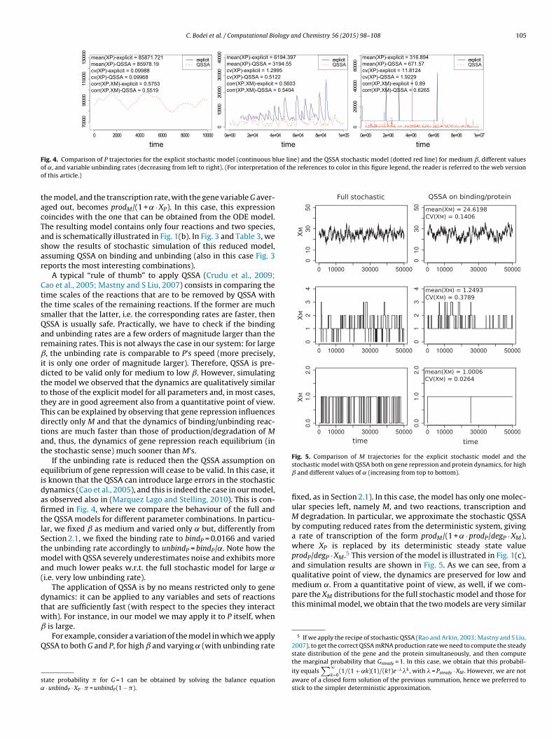
is large.For example, consider a variation of the model in which we apply

SSA to both G and P, for high ˇ and varying ˛ (with unbinding rate

tate probability � for G = 1 can be obtained by solving the balance equation· unbindP · XP · � = unbindP(1 − �).

Fig. 5. Comparison of M trajectories for the explicit stochastic model and thestochastic model with QSSA both on gene repression and protein dynamics, for highˇ and different values of ˛ (increasing from top to bottom).

fixed, as in Section 2.1). In this case, the model has only one molec-ular species left, namely M, and two reactions, transcription andM degradation. In particular, we approximate the stochastic QSSAby computing reduced rates from the deterministic system, givinga rate of transcription of the form prodM/(1 + ˛ · prodP/degP · XM),where XP is replaced by its deterministic steady state valueprodP/degP · XM.5 This version of the model is illustrated in Fig. 1(c),and simulation results are shown in Fig. 5. As we can see, from aqualitative point of view, the dynamics are preserved for low and

5 If we apply the recipe of stochastic QSSA (Rao and Arkin, 2003; Mastny and S Liu,2007), to get the correct QSSA mRNA production rate we need to compute the steadystate distribution of the gene and the protein simultaneously, and then computethe marginal probability that Gsteady = 1. In this case, we obtain that this probabil-

ity equals∑∞

k=0(1/(1 + ˛k)(1)/(k!)e−��k , with � = Psteady · XM . However, we are not

aware of a closed form solution of the previous summation, hence we preferred tostick to the simpler deterministic approximation.

Page 9

1 logy a

faP

btuiem

3

Pbdttm

Pa(stocIeat(fstda

eefModrc

4

hotii

cms

ttgh

06 C. Bodei et al. / Computational Bio

or low and medium ˛ (Table S5). We stress that QSSA on P can bepplied only for large values of ˇ, i.e. when the correlation betweenand M is close to 1.

It is clear that the hybrid abstraction and the QSSA can be com-ined together (Crudu et al., 2009). In Fig. 3 and Table 3, we showhe results of hybrid simulation of the reduced model where QSSA issed to abstract binding and unbinding. Also in this case the dynam-

cs are essentially similar to those of the explicit model. This can bexplained following and combining the considerations we alreadyade for the two abstractions separately.

.4. Some statistical insights

Looking at the histograms of the distribution of the amounts ofand M at time t = 10, 000 s (see Figs. S2, S3, S4, S5 for the distri-utions of P) for all the models considered, we can observe that theistributions look visually quite similar. This is confirmed by statis-ically testing the difference between the empirical distributions ofhe abstract models and the empirical distribution of the stochastic

odel.In particular, we computed the histogram distance (Cao and

etzold, 2006) and we performed both a Mann-Withney test (Mannnd Whitney, 1947) and a Kolmogorov-Smirnov test (Sheskin, 2004)Tables S1, S2, S3). The histogram distance is used in Monte Carloimulation to calculate the distance between histogram functionshat approximate probability density functions of different groupf samples. The Mann-Whitney test is a non-parametric test used toheck for a significant statistical dominance between two samples.ts two-sided version can be used to check for a significant differ-nce between two populations. It is also used as a test for detectingdifference between locations (means or medians), assuming that

he two samples come from distributions with the same shape. Thetwo-samples) Kolmogorov-Smirnov test, instead, is a classical testor goodness of fit between two samples, testing the null hypothe-is that the two samples come from the same distribution (for thewo-sided case). These three tests can detect different aspects ofifferences between distributions, hence we present the results ofll of them in the Supplementary Material.

All these tests reported no significant difference between thempirical distributions for most parameter combinations. How-ver, some statistically significant differences are detected, mainlyor large values of ˛ and in relation to the hybrid approach.

oreover, the tests give different results for some combinationsf parameters (with Kolmogorov–Smirnov and Mann–Whitneyetecting more significant differences). There could be severaleasons for these differences, related to the number of samplesonsidered, or to the particular shape of the density functions.

. Discussion

Aiming at defining a rigourous strategy for building correctybrid models of biochemical systems, we studied the dynamicsf a simple and paradigmatic gene regulatory network. In this con-ext, we set up a systematic investigation for evaluating the relativemportance of different sources of noise (i.e. the reactions compos-ng the model) in determining the overall behaviour.

The results of this analysis allowed us to identify which of theonsidered reactions can be specified through a deterministic for-alisms, while preserving the accuracy of the corresponding fully

tochastic model in reproducing the described dynamics.First, we identified two main parameters that govern the sys-

em’s behaviour, grounding on the fundamental information abouthe basic “building blocks” of the system (i.e. protein, mRNA, andene dynamics) and checking the validity of different plausibleypotheses. We also identified biologically reasonable ranges for

nd Chemistry 56 (2015) 98–108

the values of these parameters. Subsequently, in order to carryout numerical analysis, we considered several possible abstrac-tions of the exact discrete stochastic model, relating their validityto the possible values of parameters identified. The use of differ-ent abstract models also allowed us to identify the key species andinteractions that determine the overall behaviour of the system.Finally, we analysed the model quantitatively, also comparing theviability of different abstractions.

4.1. Different dynamic behaviours: role of parameters

A collection of distinct dynamic behaviours emerged, and wewere able to link (relative) values of model parameters withobserved behaviours, covering (to the best of our knowledge) thefull landscape of behaviours reported in the literature. This anal-ysis justified our assumption that feedback repression strengthand relative degradation speed are good descriptors of the net-work behaviour. We provided a quantitative analysis of the relativecontribution of various parameters to the global dynamics, cor-relating precise parameter combinations with a corresponding“behavioural phenotype”. For instance, low values of both ˛ andˇ yield the “continuous phenotype”, while high values of ˛ andˇ correspond to the “multi-modal phenotype”. It is interesting tonotice that gene expression dynamics switching from continuous tooscillating behaviours are common in biological systems and can beused as mechanisms to trigger alternative responses (Walker et al.,2010).

4.2. Different dynamic behaviours: emergence and relation tomodel abstraction

Analysing different abstract models allowed us to better clarifywhich interactions in the model are crucial for distinct behaviouralphenotypes to emerge. All the used abstractions are compared interms of computational cost and of the potential of the underlyingmodel to faithfully reproduce exact behaviours and on the deriv-ing cost/benefit ratio. We showed that while the fully continuousapproximation failed to capture relevant behaviours (as expected),a hybrid approximation scheme, where only the protein is treatedcontinuously, worked very well also for moderately low proteinnumbers. However, a discrete treatment of the protein was shownto be necessary for very small numbers in order to avoid significantloss in accuracy. We finally investigated the use of QSSAs on genedynamics and its interaction with hybrid abstraction, recoveringknown patterns in the accuracy of this approximation also for thehybrid case (Cao et al., 2005).

4.3. Noise sources

The hybrid and QSSA abstractions allowed us to selectively turnon and off the different (internal) noise sources of the system, i.e.the different reactions, by treating them as continuous or removingthem via QSSA. In this way, we were able to identify the reactionswhich are essential for producing the observed noise patterns. Ourexperimentation showed that the key reactions are those involvedin modifying the value of molecular species present in low numbersand that are slow (hence not amenable to QSSA). To analyse to whatextent noise patterns are correctly reproduced, a model describ-ing a negative feedback loop can be safely simplified abstractingaway the non-key reactions. Our methodology of screening andtargeting key reactions can be generalised to more complex mod-els. Hence, it is the intrinsic discreteness of the system (in terms of

low copy numbers of some molecular species) that drives the noisedynamics.

In summary, we systematically analysed a fully detailed discretestochastic model of a negative feedback loop, collecting interesting

Page 10

logy a

isSacto

ttburaagpa

•

•

•

•

•

apn(efitauuwaoTds

A

“CbhRC

C. Bodei et al. / Computational Bio

nsights on its dynamics; in this respect, our results can be con-idered an extension of the ones presented in (Marquez Lago andtelling, 2010). Furthermore, we precisely analysed the impact ofbstractions on the viability of model analysis. By systematicallyomparing the exact model with its abstractions, we highlightedhe key interactions that determine the different behavioural phen-types exhibited by the model.

We believe that our methodology, i.e. a preliminary computa-ional screening for identifying the key structural parameters andhe regions in which different abstractions are applicable, followedy an extensive computational analysis, allows us to gain a deepnderstanding of the model behaviour and, at the same time, iteduces the overall computational effort compared to a more blindnd extensive exploration of the parameter space. In this sense, ourpproach can be extended to a thorough analysis of more complexenetic networks. On a more general level, the methodology pro-osed here for the study of feedback loops is based on the followingssumptions and considerations:

fully discrete stochastic models are the most reliable and can beused as “benchmarks” for the evaluation of alternative models;a complete and detailed landscape of parameter values must bedetermined and tested for each proposed model;it is important to identify the “hot points” in control structures, i.e.the key points for the regulation dynamics. Furthermore, for eachcontrol point, it is crucial to investigate to which extent the dif-ferent approximations capture the emerging behaviours, possiblyusing deductive arguments;the best trade-off between computational costs and biologicalfaithfulness is to be found in hybrid models preserving such “hotpoints”;large genetic networks may be studied by exploiting an extensiveanalysis of the simpler modules composing them. In particular,the noise properties of simple feedback mechanisms of geneticnetworks and a precise characterisation of the validity of hybridand QSSAs can be used to construct accurate abstract models ina modular way.

An interesting extension of this work would be the definition of(semi)-automatic procedure which, following the analysis stepsresented here, will aid in building hybrid models of biologicaletworks. Such methodology should proceed with an attempt tosemi-)automate parameters and (especially) “hot points” searchxploiting modularity and it would have as ultimate goal the identi-cation of the “right” level of abstraction of a network, with respecto the fully discrete stochastic model. This approach should produceclassification of relevance/weight of each point in the overall eval-ation of the chosen level of abstraction: a classification certainlyseful from a biological point of view, but very difficult to realiseithout a systematic modus operandi. In this setting, it would be

lso interesting to investigate to what extent the proposed method-logy can be extended to preserve specific classes of behaviours.his would in principle allow to select for abstractions exhibiting aynamics that closely relates to the expected dynamics of the realystem under consideration.

cknowledgements

Davide Chiarugi acknowledges the support of the FlagshipInterOmics” project (PB.P05), supported by the Italian MIUR andNR organizations. Maria Luisa Guerriero was partially supported

y Science Foundation Ireland research grant SFI 13/IF/B2792;er current affiliation is AstraZeneca, Cambridge, UK. Alessandroomanel’s contribution was partially supported by the ABSTRACT-ELL ANR-Chair of Excellence.

nd Chemistry 56 (2015) 98–108 107

Appendix A. Supplementary data

Supplementary data associated with this article can be found,in the online version, at http://dx.doi.org/10.1016/j.compbiolchem.2015.04.004

References

Alberts, B., Johnson, A., Lewis, J., Raff, M., Roberts, K., Walter, P., 2002. Mole. Biol. Cell.Garland Science.

Balázsi, G., van Oudenaarden, A., Collins, J.J., 2011. Cellular decision making andbiological noise: from microbes to mammals. Cell 144 (6), 910–925.

Bartholomay, A.F., 1958. Stochastic models for chemical reactions. Bull. Math. Bio-phys. 20 (3), 175–190.

Becksei, A., Séraphin, B., Serrano, L., 2001. Positive feedback in eukaryotic genenetworks: cell differentiation by graded binary response conversion. EMBO J.20 (10), 2528–2535.

Bortolussi, L., Policriti, A., 2009. Hybrid semantics of stochastic programs withdynamic reconfiguration. In: Proceedings of CompMod’09, pp. 63–76.

Bortolussi, L., Policriti, A., 2013. (Hybrid) automata and (stochastic) programs: thehybrid automata lattice of a stochastic program. J. Logic Comput. 23 (4), 761–798.

Burden, R.L., Faires, J.D., 2005. Numerical Analysis. Thomson Brooks/Cole.Cao, Y., Petzold, L., 2006. Accuracy limitations and the measurement of errors in the

stochastic simulation of chemically reacting systems. J. Comput. Phys. 212 (1),6–24.

Cao, Y., Gillespie, D.T., Petzold, L.R., 2005. The slow-scale stochastic simulation algo-rithm. J. Chem. Phys. 122 (1), 014116.

Chabot, J.R., Pedraza, J.M., Luitel, P., van Oudenaarden, A., 2007. Stochastic geneexpression out-of-steady-state in the cyanobacterial circadian clock. Nature 450(7173), 1249–1252.

Costa, O.L.V., Dufour, F., 2008. Stability and Ergodicity of Piecewise DeterministicMarkov Processes. SIAM J. Control Optim. 47, 1053–1077.

Crudu, A., Debussche, A., Radulescu, O., 2009. Hybrid stochastic simplifications formultiscale gene networks. BMC Syst. Biol. 3, 89.

Dauxois, T., Di Patti, F., Fanelli, D., McKane, A.J., 2009. Enhanced stochastic oscilla-tions in autocatalytic reactions. Phys. Rev. E: Stat. Nonlinear Soft Matter Phys.79, 036112.

Davis, M.H.A., 1993. Markov Models and Optimization. Chapman & Hall.Elowitz, M.B., Levine, A.J., Siggia, E.D., Swain, P.S., 2002. Stochastic gene expression

in a single cell. Science 297 (5584), 1183–1186.Gibson, M., Bruck, J., 2000. Efficient exact simulation of chemical systems with many

species and many channels. J. Phys. Chem. 104 (9), 1876–1889.Gillespie, D.T., Petzold, L., 2006. Numerical simulation for biochemical kinetics. In:

Ch. System Modelling in Cellular Biology. MIT Press, pp. 1–29.Gillespie, D., 1977. Exact stochastic simulation of coupled chemical reactions. J. Phys.

Chem. 81 (25), 2340–2361.Gillespie, D.T., 2000. The chemical Langevin equation. J. Chem. Phys. 113 (1),

297–306.Golding, I., Paulsson, J., Zawilski, S.M., Cox, E.C., 2005. Real-time kinetics of gene

activity in individual bacteria. Cell 123 (6), 1025–1036.Hoops, S., Sahle, S., Gauges, R., Lee, C., Pahle, J., Simus, N., Singhal, M., Xu, L., Mendes,

P., Kummer, U., 2006. COPASI: a COmplex PAthway SImulator. Bioinformatics22 (24), 3067–3074.

Hume, D.A., 2000. Probability in transcriptional regulation and its implicationsfor leukocyte differentiation and inducible gene expression. Blood 96 (7),2323–2328.

Lillacci, G., Khammash, M., 2010. Parameter estimation and model selection in com-putational biology. PLoS Comput. Biol. 6 (3), e1000696.

Mann, H.B., Whitney, D.R., 1947. On a test of whether one of two random variablesis stochastically larger than the other. Ann. Math. Stat. 18 (1), 50–60.

Mantzaris, N.V., 2007. From single-cell genetic architecture to cell populationdynamics: quantitatively decomposing the effects of different population het-erogeneity sources for a genetic network with positive feedback architecture.Biophys. J. 92 (12), 4271–4288.

Marquez Lago, T.T., Stelling, J., 2010. Counter-intuitive stochastic behavior of simplegene circuits with negative feedback. Biophys. J. 98 (9), 1742–1750.

W.E., Liu, D., Vanden-Eijnden, E., 2005. Nested stochastic simulation algorithm forchemical kinetic systems with disparate rates. J. Chem. Phys. 123, 194107.

W.E., Liu, D., Vanden-Eijnden, E., 2007. Nested stochastic simulation algorithms forchemical kinetic systems with multiple time scales. J. Comput. Phys. 221 (1),158–180.

Mastny, E.A., Haseltine, E.L., Rawlings, J.B., 2007. Two classes of quasi-steady-statemodel reductions for stochastic kinetics. J. Chem. Phys. 127 (9), 094106.

McQuarrie, D., 1967. Stochastic approach to chemical kinetics. J. Appl. Probab. 4 (3),413–478.

Murphy, K.F., Adams, R.M., Wang, X., Balázsi, G., Collins, J.J., 2010. Tuning and con-trolling gene expression noise in synthetic gene networks. Nucleic Acids Res. 38(8), 2712–2726.

Novic, A., Weiner, M., 1957. Enzyme induction as an all-or-none phenomenon. Proc.

Natl. Acad. Sci. U. S. A. 43 (7), 553–566.

Pahle, J., 2009. Biochemical simulations: stochastic, approximate stochastic andhybrid approaches. Brief Bioinform. 10 (1), 53–64.

Peccoud, J., Ycart, B., 1995. Markovian modelling of gene-product synthesis. Theor.Popul. Biol. 48 (2), 222–234.

Page 11

1 logy a

R

R

R

R

R

R

R

R

R

08 C. Bodei et al. / Computational Bio

aj, A., van Oudenaarden, A., 2008. Nature, nurture, or chance: stochastic geneexpression and its consequences. Cell 135 (2), 216–226.

aj, A., van Oudenaarden, A., 2009. Single-molecule approaches to stochastic geneexpression. Annu. Rev. Biophys. 38, 255–270.

aj, A., Peskin, C.S., Tranchina, D., Vargas, D.Y., Tyagi, S., 2006. Stochastic mRNAsynthesis in mammalian cells. PLoS Biol. 4 (10), e309.

aj, A., Rifkin, S.A., Andersen, E., van Oudenaarden, A., 2010. Variabilityin gene expression underlies incomplete penetrance. Nature 463 (7283),913–918.

amaswamy, R., Sbalzarini, I., 2010. A partial-propensity variant of the composition-rejection stochastic simulation algorithm for chemical reaction networks. J.Chem. Phys. 132 (4), 044102.

ao, C.V., Arkin, A.P., 2003. Stochastic chemical kinetics and the quasi-steady stateassumption: application to the Gillespie algorithm. J. Chem. Phys. 118 (11),4999–5010.

athinam, M., Petzold, L.R., Cao, Y., Gillespie, D.T., 2003. Stiffness in stochastic chem-ically reacting systems: the implicit tau-leaping method. Journal of ChemicalPhysics 119 (24), 12784–12794.

esat, H., Petzold, L., Pettigrew, M.F., 2009. Kinetic modeling of biological systems.Methods Mol. Biol. 541 (10), 311–335.

oss, I.L., Browne, C.M., Hume, D.A., 1994. Transcription of individual genes ineukaryotic cells occurs randomly and infrequently. Immunol. Cell Biol. 72 (2),177–185.

nd Chemistry 56 (2015) 98–108

Salis, H., Kaznessis, Y., 2005. Accurate hybrid stochastic simulation of a system ofcoupled chemical or biochemical reactions. J. Chem. Phys. 122 (5), 54103.

Salis, H., Sotiropoulos, V., Kaznessis, Y.N., 2006. Multiscale Hy3S: hybrid stochasticsimulation for supercomputers. BMC Bioinform. 7, 93.

Sheskin, D.J., 2004. Handbook of Parametric and Nonparametric Statistical Proce-dures, 3rd ed. Chapman & Hall.

Stamatakis, M., Zygourakis, K., 2010. A mathematical and computational approachfor integrating the major sources of cell population heterogeneity. J. Theor. Biol.266 (1), 41–61.

Stamatakis, M., Zygourakis, K., 2011. Deterministic and stochastic population levelsimulations of an artificial lac operon genetic network. BMC Bioinform. 12, 301.

Stekel, D.J., Jenkins, D.J., 2008. Strong negative self regulation of prokaryotic tran-scription factors increases the intrinsic noise of protein expression. BMC Syst.Biol. 2, 6.

Trivedi, K.S., Kulkarni, V.G., 1993. FSPNs: fluid stochastic Petri nets. In: Applicationand Theory of Petri Nets., pp. 24–31.

Vogel, U., Jensen, K.F., 1994. The RNA chain elongation rate in Escherichia colidepends on the growth rate. J. Bacteriol. 176 (10), 2807–2813.

Walker, J.J., Terry, J.R., Tsaneva-Atanasova, K., Armstrong, S.P., McArdle, C.A., Light-man, S.L., 2010. Encoding and decoding mechanisms of pulsatile hormonesecretion. J. Neuroendocrinol. 22 (12), 1226–1238.

Zhou, G.-Q., Zhong, W.-Z., 1982. Diffusion-controlled reactions of enzymes. Eur. J.Biochem. 128 (2-3), 383–387.