1-s2.0-S0920410514000102-main

Author's Accepted Manuscript

Numerical Solution of the Nonlinear Diffusiv-ity Equation in Heterogeneous Reservoirswith Wellbore Phase Redistribution

Kourosh Khadivi, Mohammad Soltanieh

PII: S0920-4105(14)00010-2DOI: http://dx.doi.org/10.1016/j.petrol.2014.01.004Reference: PETROL2584

To appear in: Journal of Petroleum Science and Engineering

Received date: 22 January 2013Accepted date: 5 January 2014

Cite this article as: Kourosh Khadivi, Mohammad Soltanieh, NumericalSolution of the Nonlinear Diffusivity Equation in Heterogeneous Reservoirswith Wellbore Phase Redistribution, Journal of Petroleum Science and Engineering,http://dx.doi.org/10.1016/j.petrol.2014.01.004

This is a PDF file of an unedited manuscript that has been accepted forpublication. As a service to our customers we are providing this early version ofthe manuscript. The manuscript will undergo copyediting, typesetting, andreview of the resulting galley proof before it is published in its final citable form.Please note that during the production process errors may be discovered whichcould affect the content, and all legal disclaimers that apply to the journalpertain.

www.elsevier.com/locate/petrol

http://dx.doi.org/10.1016/j.petrol.2014.01.004






Numerical Solution of the Nonlinear Diffusivity Equation in Heterogeneous

Reservoirs with Wellbore Phase Redistribution

Kourosh Khadivi and Mohammad Soltanieh*

Department of Chemical and Petroleum Engineering

Sharif University of Technology, Azadi Ave., P.O. Box 11155-9465, Tehran, Iran.

* Corresponding author, Email: [email protected]

Abstract

We consider the application of the Finite Element Method (FEM) for numerical

pressure transient analysis under conditions where no reliable analytical solution is

available. Pressure transient analysis is normally based on various analytical solutions of

the linear one-dimensional diffusion equation under restrictive assumptions about the

formation and its boundaries. For example, the formation is either assumed isotropic or a

restrictive a priori assumption is made about its heterogeneity. The wellbore storage

effect is also often considered without regard to the possibility of phase redistribution. In

many practical situations such restrictions are not justified and analytical solutions do not

exist. Here we present a numerical solution of the nonlinear diffusion equation based on

the FEM that can be used without any restrictive a priori assumptions. Through the use

of the weak formulation of the FEM, solution can be obtained for a heterogeneous

medium with discontinuous or nonlinear properties. The weak formulation also enables

the handling of time dependent boundary conditions and hence problems involving

wellbore storage with significant phase redistribution. The speed and accuracy of the

numerical technique is first confirmed by comparison with simple test cases that admit an

analytical solution. The practical utility of the proposed method is then demonstrated for

a number of test cases that involve discontinuous and nonlinear formation properties

and/or wellbore storage with phase redistribution.

Keywords: Finite Element Method, Weak Formulation, Wellbore Storage, Phase

Redistribution, Heterogeneity, Pressure Transient Analysis.

1. Introduction

The pressure transient response of the reservoir is a widely used method for reservoir

characterization. However, the early time portion of such data sometimes is infected by

wellbore effects. To discriminate the reservoir portion from the wellbore portion and

extracting a true reservoir parameter, a wellbore model is required. Currently, there are

three types of flow models which can be used for modeling fluid flow in the wellbore;

empirical correlations, homogeneous models and mechanistic models (Shi et al. 2005a).

Empirical correlations are based on matching of experimental data and their range of

applicability are generally limited to the range of variables and the particular geometry

used in the experiments (Duns et al., 1963; Hagedorn and Brown, 1965; Orkiszewski,

1967; Aziz et al., 1972; and Beggs et al., 1973; Ansari et al., 1994). Homogeneous

models that sometimes are called drift-flux models, assume that a single-phase fluid

flows in the wellbore and the properties of this fluid is represented by a mixture of

properties (Shi et al. 2005a; Shi et al. 2005b). Both empirical correlations and

homogeneous models have been developed mainly for steady state multiphase flow in the

wellbore. However, during the well test, the wellbore condition is generally kept in

single-phase flow and pressure is always changing by time. Therefore, such wellbore

flow models are no longer applicable for pressure transient analysis. Mechanistic models;

however, are based on the fundamental conservation laws of mass and momentum

transfer e.g. Navier-Stokes differential equations. Although, they are accurate and reliable

models and can be used in transient condition; however, the computational burden is

significant to solve them and to get reliable solutions. They often encounter convergence

problems and the computation time is remarkably long. For instance, initializing Navier-

Stokes equations and establishing velocity field in the well, sometimes takes a longer

time than solving the diffusion equation in the reservoir. The computation time becomes

noticeable especially when the coupled wellbore-reservoir model should be executed for

many times to estimate reservoir parameters (Pourafshary et al. 2009; Khadivi et al.,

2013).

An alternative approach, which is often used for pressure transient analysis, is

considering the well as a boundary condition instead of a separate model. The accuracy

of this method in representing the wellbore dynamic depends on the equation that is used

as the boundary condition. This type of well modeling is fast and reliable to represent

wellbore dynamics in various well conditions. The overall goal of this work is developing

an efficient and fast numerical procedure to handle reservoir heterogeneity in the

presence of wellbore effects.

2. Problem Formulation

In this section, we briefly review the governing flow equations in the reservoir and

give the associated weak form.

2.1 Governing Equations

Most of the theoretical treatments of pressure transient analysis in well testing

consider a well situated in a porous medium of infinite radial extent and assume that the

fluids flow to a central cylinder (the well) that is normal to two parallel, impermeable

planar barriers. The theoretical analysis is based on simplified solutions of the continuity

equation in the porous medium:

. 0 (1)

where is the density of the formation fluid, is porosity, is the fluid velocity vector

and is time. Flow of the fluid in the porous media is assumed to follow the form of

D’Arcy’s law,

. (2)

Here, is the superficial Darcy velocity vector, is the reservoir pressure, and ρ

are the fluid viscosity and density, g is the magnitude of the acceleration due to gravity,

is a unit vector in the direction over which gravity acts and is the symmetric and

positive definite 3D permeability tensor, respectively. Substituting Eq. (2) into the

continuity equation yields,

. 0. (3)

Taking the fluid and rock compressibility as constant, and

, leads to a diffusion equation that describes the temporal and

spatial pressure changes in the 3D reservoir,

. 0, (4)

where is the total compressibility.

It is assumed that the top and bottom surfaces of the reservoir layer are sealed and a

uniform (either constant pressure or no flow) boundary condition is imposed at the outer

limit of the reservoir. It is further assumed that there is no variation in direction (radial

symmetry) and the reservoir is long enough to be assumed as a single thin layer reservoir.

Then with such boundary conditions, the problem geometrically and physically is a one-

dimensional symmetric problem.

10 5

The analysis of the measured pressure transient is based on the solution of Eq. (5)

subject to suitable boundary conditions. In the case of an isotropic reservoir the following

initial and boundary conditions are often adopted. As the initial condition, the pressure in

the reservoir is assumed to be uniform at a given initial value, , 0 . For the

outer boundary condition, the pressure gradient at the outer limit of the reservoir is zero

at all times, , 0 . This may mean that the pressure transient will not reach to

the end of the reservoir, the so-called infinite acting reservoir. Alternatively, for long

durations or small radius reservoirs it may mean that the reservoir is closed at its outer

limit, . 0 .

Depending on the assumptions made regarding behavior within the wellbore, three

major alternatives are used:

I) Negligible Wellbore Storage: accumulation of fluid within the wellbore is ignored all

together and the fluid issuing from the reservoir is withdrawn directly into the

wellbore, the so-called line source well

· 2 0 , 6

where is the wellbore radius and is the unit vector normal to the boundary. In the

simplest case of no wellbore storage, the diffusivity equation in a one-dimensional

homogeneous reservoir admits a closed form analytical solution based on exponential

integrals (Theis 1935; Crank 1975; Carslaw and Jeager, 1959; Bourdet, 2002).

II) Wellbore Storage: accumulation of fluid in the wellbore is considered and the flux is

assumed to consist of that coming from the well itself and that issuing from the

reservoir,

·1

2 0 7

where is the instantaneous bottom-hole flowing pressure and is the wellbore

storage coefficient. In case of wellbore storage with no phase redistribution, the

diffusivity equation remains linear and an analytical solution can be obtained in the

Laplace domain (Van Everdingen and Hurst 1949; Gringarten et al. 1979; Bourdet et

al. 1983 and Bourdet et al. 1989), which can be readily inverted with the aid of the

Stehfast algorithm (1970).

III) Wellbore Storage with Phase Redistribution: in many cases expansion and

contraction of the fluid in the wellbore is accompanied with redistribution of oil and

gas within the wellbore due to gravity effect. This highly nonlinear phase

redistribution effect occurs frequently in the build-up test because gas bubbles tend to

migrate upward and oil slugs tend to migrate downward under the action of gravity.

The inner-boundary condition in this case is taken as:

·1

2⁄ 0 8

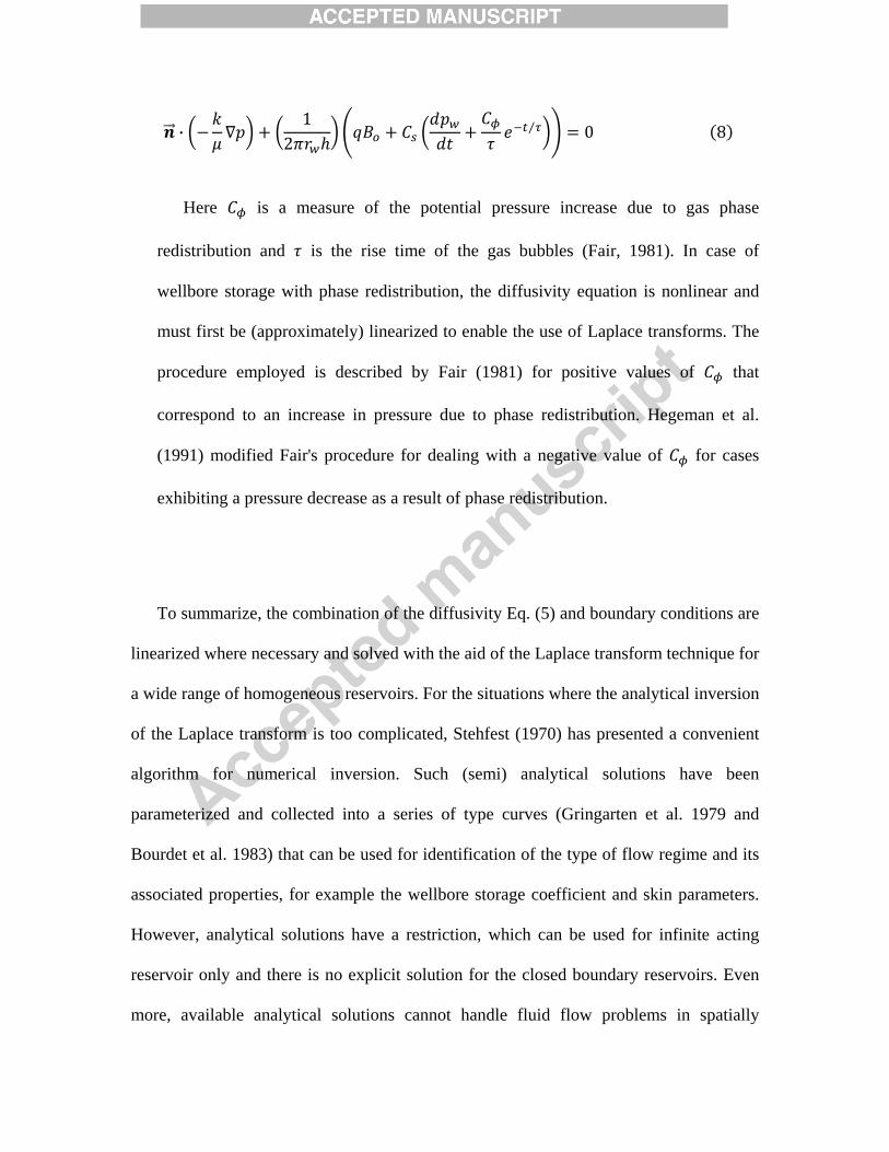
Here is a measure of the potential pressure increase due to gas phase

redistribution and is the rise time of the gas bubbles (Fair, 1981). In case of

wellbore storage with phase redistribution, the diffusivity equation is nonlinear and

must first be (approximately) linearized to enable the use of Laplace transforms. The

procedure employed is described by Fair (1981) for positive values of that

correspond to an increase in pressure due to phase redistribution. Hegeman et al.

(1991) modified Fair's procedure for dealing with a negative value of for cases

exhibiting a pressure decrease as a result of phase redistribution.

To summarize, the combination of the diffusivity Eq. (5) and boundary conditions are

linearized where necessary and solved with the aid of the Laplace transform technique for

a wide range of homogeneous reservoirs. For the situations where the analytical inversion

of the Laplace transform is too complicated, Stehfest (1970) has presented a convenient

algorithm for numerical inversion. Such (semi) analytical solutions have been

parameterized and collected into a series of type curves (Gringarten et al. 1979 and

Bourdet et al. 1983) that can be used for identification of the type of flow regime and its

associated properties, for example the wellbore storage coefficient and skin parameters.

However, analytical solutions have a restriction, which can be used for infinite acting

reservoir only and there is no explicit solution for the closed boundary reservoirs. Even

more, available analytical solutions cannot handle fluid flow problems in spatially

heterogeneous reservoirs with significant phase redistribution effect in the wellbore.

Spatial variation of porosity and permeability in the reservoir can result in a highly

nonlinear diffusivity equation. The problem is further complicated by the need to account

for non-ideal wellbore storage effects and phase redistribution. However, this problem

can be solved numerically and leads to the more modern topic of “numerical well

testing”, which is capable of dealing with heterogeneous reservoirs directly.

2.2 FEM and Weak Form

In pressure transient analysis, we seek the pressure response such that it satisfies the

pressure diffusivity equation, e.g. 0 in a ‘domain’ (volume or radius), Ω, together

with certain boundary conditions, e.g. 0, on the boundaries, Γ, of the domain.

The FEM is one of the numerical approximations that seeks the solution in the

approximation form. In the FEM, a complex region defining a continuum is discretized

into simple geometric shapes called elements. The properties and the governing

relationships are assumed in terms of, usually fairly simple, approximating shape

functions over the individual elements and expressed mathematically in terms of the

desired unknown values at specific points in the element called nodes. An assembly

procedure is then used to link the individual elements within a given region. The

assembly procedure relates the local nodes of an element to the global node scheme and

relates the solution on neighboring elements together. Since the shape functions are

usually defined locally for elements or subdomains, therefore, the properties of discrete

systems can be recovered if the approximating equations are cast in an integral form.

Therefore, we seek to cast the equations in the integral form. The pressure transient

response of a 3D reservoir can be obtained by integrating over the reservoir volume

Ω and across the boundaries, Γ.

Ω . Γ 0.Ω (9)

For a fixed (independent of ) volume and, under suitable conditions of smoothness

of the intervening quantities, we can apply the Gauss’ theorem:

· ΩΩ . Γ (10)

to obtain,

· Ω 0Ω (11)

For the integral expression to be zero for any volume Ω, the integrand must be zero.

· 0 (12)

This implies an excessive “smoothness” of the true solution. For this reason, it is

sometimes called the strong or differential form of the equation. The familiar finite

difference method (FDM) uses the strong or differential form of the governing equations,

which requires strict adhesion to the smoothness property of the variables and is ill suited

to heterogeneous media. In contrast, the finite volume and finite element methods deal

with the integral form directly and obviate the need for strict smoothness and spatial

continuity of the variables. An alternative integral form can be obtained by the method of

weighted residuals. Multiplying Eq. (11) by a weight function and integrating over

the reservoir volume Ω we obtain

· Ω 0Ω (13)

If Eq. (13) is satisfied for any weight function , then Eq. (13) is equivalent to the

differential form Eq. (12). The smoothness requirements on can be relaxed by

applying the Gauss’ theorem to Eq. (13) to obtain

· Ω . Γ 0Ω (14)

This is known as the weak form [Peir´o and Sherwin, 2005; Zienkiewicz et al., 2005]

of the diffusivity equation and does not demand the smoothness of the variables involved.

This is the essence of the finite element method and can be applied for any linear or

nonlinear partial differential equation (PDE), where the choice of the weight function

defines the type of finite element scheme used.

2.3 Model Characteristics

A schematic of numerical model is presented in Figure 1. The reservoir is assumed to

be one dimensional (vertically homogeneous) but it can be heterogeneous in radial

direction as shown in Figure 1. This behavior is observed in typical damaged reservoirs

due to near wellbore skin [Van Everdingen, 1953; Hawkins, 1956]. The reservoir is

divided into two zones; near wellbore damaged zone and undamaged zone. The wellbore

radius is 0.1 m, the outer reservoir radius is 1,000 m and the interior boundary between

the zones is 1.0 m. In a homogeneous case, permeability as well as porosity is similar in

either zone; however, in a heterogeneous case, they are different. The weak formulation

of the FEM enables the handling of porous medium with sharp (discontinuous) variations

in rock properties in heterogeneous reservoirs. Accurate and stable numerical results are

obtained by using a sufficiently fine mesh close to the perforations. The performance of

numerical model is verified in the next section by comparing with the analytical or semi-

analytical solutions.

3. Verification

In this section, the performance of the new numerical solution is demonstrated in

three cases. In addition, to verify the performance of numerical solution, the results are

compared with analytical or semi-analytical solutions.

3.1 Case 1: Homogeneous Reservoir without any Wellbore Storage and Skin

Effects

We consider a central well that is fully perforated over the reservoir layer with a

constant rate drawdown of 31.8 m3/day (200 stb/day). The reservoir is a very large

homogenous reservoir, where the pressure transient response does not reach the outer

boundary and acts as an infinite acting reservoir. The basic reservoir fluid and reservoir

characteristics for this model are summarized in Table 1. In order to validate the

numerical model, the numerical pressure transient response of a homogeneous reservoir

without any effects of wellbore storage and skin is compared with its analytical solution

as shown in Figure 2. Figure 2 compares the dimensionless pressure of a well in an

infinite acting reservoir. In this case, the numerical FEM solution using Eq. (6) at the

wellbore and the closed form analytical solution are virtually indistinguishable in middle

time and late time regions. There is a good match at the middle and late times; however,

pressure transient responses derived by analytical and numerical methods are different at

the early time region. The reason for this discrepancy is due to an unrealistic assumption

in deriving the analytical procedure, which assumes the well can be represented as a

point. The so-called well model is recognized as the line source. The line source

approximation assumes that the wellbore radius to be vanishingly small. Although

physically this is acceptable because the dimension of the wellbore is so small compared

to the radius of the volume drained by the well; however, in mathematical point of view,

it may not be true. The discrepancy of numerical and analytical solutions in the early time

is highlighted by using log-log plot of dimensionless pressure and dimensionless pressure

derivatives as shown in Figure 3. Mueller and Whitherspoon (1965) investigated the

validity of this solution in the case of finite wellbore radius and concluded that the line

source solution is an excellent approximation within one percent for all values of when

50 and for 20 then 0.5. As we will see later, generally during this time

the pressure transient response of the well is mainly affected by the wellbore storage

effect. Furthermore, the computation time required for the FEM solution is not so

different from that required for evaluating the closed form analytical solution.

3.2 Case 2: Homogeneous Reservoir with Wellbore Storage and Skin Effects

Next we consider a homogeneous reservoir with ideal wellbore storage. In this case

the well is open or closed on the surface and there is the possibility of expansion or

contraction of the wellbore fluid but no phase redistribution. This characteristic flow

regime, called pure wellbore storage effect, can last from a few seconds to a few minutes

(Bourdet, 2002) and appears like a hump at early times of the derivative plot. This case

admits a solution in the Laplace domain that can be inverted using the Stehfest algorithm

(1970). The FEM solution is obtained using Eq. (7) as the inner boundary condition. The

results are compared in Figure 4 and are practically indistinguishable. Furthermore, the

FEM solution is delivered with a computation time faster than that required by the

Stehfest algorithm (1970). The wellbore storage effect is observed in the early portions

of the pressure response and appears as a hump on the log-log plot that gradually

vanishes at later times where the flow becomes purely radial. In addition, the

dimensionless pressure obtained using the Stehfest method and the numerical solution are

compared with the data reported by Agarwal et al. (1970) for wells with different storage

coefficients and skin factors in Figure 5. Again, there is excellent agreement between the

semi-analytical and FEM solutions and both methods fit the data well.

3.3 Case 3: Homogeneous Reservoir with Phase Redistribution and Skin Effects

We now turn to an example involving non-ideal wellbore storage effects. In this case

the well is shut in on the surface and a phase redistribution phenomenon is assumed to

occur during wellbore storage. The inner boundary condition is now taken as Eq. (8) that

allows for phase redistribution. Again, the solution of the diffusivity equation in the

Laplace domain is too complicated for analytical inversion. The inverse Laplace

transforms were calculated numerically using the Stehfest algorithm (1970). The results

obtained are compared with the FEM solution in Figures 6 and 7 that show excellent

agreement. Depending on the value of and , the wellbore storage hump and its

duration on the log-log plot vary in the early stages of the pressure response. A number of

data also for buildup tests in wells exhibiting phase redistribution have been reported by

Fair (1981), which are superimposed on Figures 6 and 7 for comparison purposes.

4. Application

The results presented above confirm the accuracy and reliability of the FEM solution.

In this section, the application of the new numerical solution in pressure transient analysis

of heterogeneous reservoirs is highlighted. It is well understood that wellbore storage and

phase redistribution effects have major influences on the early time portion of the

pressure transient response. Skin, for example, can change the shape of dimensionless

pressure and dimensionless pressure derivative as depicted on Figure 8. Skin in fact

delays the establishment of radial flow in undamaged zone. Dimensionless wellbore

storage (CD) influences the shape of hump on both dimensionless pressure and

dimensionless derivative plots as shown in Figure 9. Dimensionless phase redistribution

pressure parameter ( ) and, dimensionless phase redistribution time parameter ( )

have distinct influences on both dimensionless pressure and dimensionless derivative

plots as shown on Figures 10 and 11, respectively. At large values of dimensionless

phase redistribution pressure parameter ( ), a "gas hump" appears on dimensionless

pressure (Fair, 1981) and at small values; the phase redistribution diminishes (Figure 10).

In contrast, the dimensionless phase redistribution time parameter ( ) dumps the phase

redistribution effect at large values and, induces oscillation and instability in the

dimensionless pressure at small values (Figure 11). As far as major differences are seen

on pressure transient responses by variations of the above parameters, the numerical

reservoir model is sensitive and such sensitivity can be used for parameter estimation.

Therefore, these parameters can be parameterized in the model and determined by

matching the pressure response of the numerical model with the experimental pressure

response using nonlinear regression technique [Gill et al., 1981].

Although the results presented above confirm the accuracy and reliability of the FEM

solution, they are obtained for simple and ideal cases, in which both the porosity and

permeability are spatially uniform (except that of skin case). Now let's see the FEM

performance in cases that there is no analytical solution for them.

4.1 Case 4: A Radially Heterogeneous Closed System with Phase Redistribution

and Skin Effects

Consider an important practical case of radial heterogeneity in a closed boundary

reservoir. In such a heterogeneous reservoir, porosity is assumed to be vertically

homogeneous but exhibits radial deterioration along the reservoir radius in undamaged

zone. In addition, permeability in correlation with porosity deteriorates exponentially

along the reservoir radius. A schematic of such heterogeneity is illustrated in Figure 12.

This behavior can be observed in typical channel bars in deltaic environment [Nichols

Gary, 2009; Gastaldo and Huc, 1992; Reading, 1996]. In particular, the porosity is

assumed to deteriorate linearly with radial distance from well center, also the

permeability is assumed to be locally isotropic, , and taken as an

exponential function of the local porosity,

0.20 1.010 4 ; 5.066 20 .

Skin factor is 1 and other properties of reservoir fluid and reservoir characteristics for

this example are summarized in Table 1. Consider a closed boundary reservoir with

heterogeneity mentioned in Figure 12, and the phase redistribution effect in the wellbore,

and then the reservoir is drawing down for 11.6 days at a constant rate of 31.8 m3/day

(200 bbl/day). Figures 13a and 13b show the semi-log and log-log plots of pressure and

pressure derivative of this well, respectively. They also show the sensitivity of pressure

and derivative of pressure with respect to variations of skin. Different shapes of pressure

and the derivative of pressure are observed by changing skin. Skin factor mainly affects

the early time region of pressure transient response of well; however, the middle time

region in this case, which is representation of the flow regime in undamaged zone does

not show a stable flow regime (Figure 13b). The pressure response of such a

heterogeneous reservoir is quite complicated and precludes the use of usual procedures

for detecting radial flow regions developed for homogeneous reservoirs. Evidently, the

pressure transient analysis in such heterogeneous reservoirs and the detection of the

spatial heterogeneity require the development of new techniques to solve highly

nonlinear inverse problems.

A numerical well test procedure capable of capturing the radial heterogeneity is

readily established. The porosity can be parameterized as, , and the

permeability can be parameterized as, exp . and are representing

porosity and permeability at the wellbore so they can readily be found from either core or

log data. The sensitivities of the numerical model to variations of and are

demonstrated in Figures 14 and 15, respectively. Figures 14 and 15 show the influences

of and on pressure and pressure derivative response of the well, respectively. In

contrast to skin factor, which affects the early time region, and have major

influences on the middle time region of the well pressure transient response.

The parameters and are key elements in spatial variations of porosity and

permeability in this type of heterogeneous reservoir. Therefore, reservoir characterization

in such cases can proceed by searching for and . However, finding and is not

an easy task because of inherent nonlinearity of this problem due to porosity-permeability

interrelationship, but the sensitivity of pressure transient response of the well with respect

to skin, and may offer a test procedure for finding skin, and simultaneously.

Therefore, the constant parameters of skin, and can be determined by matching the

pressure response of the numerical FEM model with the experimental pressure response

using a nonlinear regression technique [Gill et al., 1981]. This technique is a reliable

approach for solving highly nonlinear and often ill-posed inverse problems [Kenneth

Levenberg, 1944; Donald Marquardt, 1963].

5. Conclusions

We presented a numerical solution for the nonlinear diffusion equation based on the

finite element method (FEM) that can be used without any restrictive a priori

assumptions. Through the use of the weak formulation of the FEM, the solution can be

obtained for heterogeneous media with discontinuous or nonlinear properties. The weak

formulation also enables the handling of time dependent boundary conditions and hence

problems involving wellbore storage with significant phase redistribution. The weak

formulation of the finite element method offers an accurate, reliable and fast procedure

for analyzing the pressure response of complex heterogeneous reservoirs. The response of

such reservoirs is very complex and cannot be analyzed using conventional procedures

developed for homogeneous reservoirs. The speed and accuracy of the numerical

technique is first confirmed by comparing with simple test cases that admit an analytical

solution. The practical applicability of the proposed method is then demonstrated for test

cases that involve discontinuous and nonlinear formation properties and/or wellbore

storage with phase redistribution.

We also developed a parametric numerical wellbore-reservoir model, which is a

reliable numerical well test procedure that can handle the phase redistribution in

heterogeneous reservoirs. This model is sufficiently sensitive with respect to the

parameters of phase redistribution and porosity-permeability variations. The model has

potential to be used to extract phase redistribution parameters in the wellbore and to

evaluate the porosity-permeability distributions in the radially heterogeneous reservoir,

which currently is either difficult or there is no analytical solution for them. This could be

achieved by coupling a nonlinear regression method to the numerical model. The

parameters can be extracted by matching the pressure response of the numerical model

with the actual pressure response. The pressure transient analysis of heterogeneous

reservoirs in the presence of phase redistribution is of great value in this development.

6. Acknowledgement

The authors, in particular K. Khadivi express sincere thanks, to his the late thesis co-

supervisor, Dr. F.A. Farhadpour, whose guidance and support made this research possible.

7. Nomenclature

Dimensionlesswellbore storage coefficient,

Dimensionless phase redistribution pressure parameter,

Rock compressibility, Lt2/m, 1/Pa

Fluid compressibility, Lt2/m, 1/Pa

Total compressibility, , Lt2/m, 1/Pa

Wellbore storage coefficient, L4t2/m, m3/Pa

Unit vector in gravity direction, L, m

The acceleration of gravity, L/t2, m/s2

Reservoir thickness, L, m

Reservoir permeability, L2, m2

Symmetric and positive definite 3D permeability tensor

Reservoir pressure, m/Lt2, Pa

Wellbore pressure, m/Lt2, Pa

Dimensionless pressure

Dimensionless phase redistribution pressure,

Flow rate, L3/t, m3/s

Radius L, m

Dimensionless radius,

External radius of drainage area L, m

Wellbore radius L, m

Skin factor

Time, t, s

Dimensionless time,

Darcy velocity (superficial) vector, L/t, m/s

Greek letters

Porosity, %

Viscosity, m/Lt, Pa.s

Fluid density, m/L3, kg/m3

Phase redistribution time parameter, s

Dimensionless phase redistribution time,

Conversion Factors

bbl × 1.589 873 E–01 = m3

cp × 1.0 E- 03 = Pa·s

ft × 3.048 E–01 = m

psi × 6.894 757 E +3 = Pa

mD×9.86927574528 E-16 = m2

8. References

1. Agarwal, R.G., Rafi Al-Hussainy, and Ramey, H.J. Jr., 1970. An Investigation of

the Well Bore Storage and Skin Effect in Unsteady Liquid Flow - I. Analytical

Treatment, - Soc. Pet. Eng. J. 279-290; Trans., AIME, 249, (1970)

2. Ansari, A.M., Sylvester, N.D., Sarica, C., Shoham, O., and Brill, j.p., 1994. A

comprehensive mechanistic model for upward two-phase flow in wellbores. SPE

Production and Facilities, Volume 9, Number 2, pp. 143-151, May 1994.

3. Aziz, K., Govicr, G. W. and Forgarasi , M., 1972. Pressure Drop in Wells

Producing Oil and Gas, J. Cdn. Pet. Tech., July-Sept., 1972.

4. Beggs, H. D. and Brill, J. P., 1973. A Study of Two-Phase Flow in Inclined Pipes,

JPT, May, 1973.

5. Bourdet, D.P., Whittle T.M., Douglas, A.A. and Pirard, Y.M., 1983. A New Set of

Type Curves Simplifies Well Test Analysis, World Oil, 95-106.

6. Bourdet D., Ayoub J.A. and Pirard Y.M., 1989. “Use of Pressure Derivative in Well

Test Interpretation”, SPEFE4 (2): 293-302. SPE-12777-P.A.

7. Bourdet, D., Well Test Analysis: The Use of Advanced Interpretation Models -

(Handbook of petroleum exploration and production), First Edition, Amsterdam,

Elsevier Science B.V., 2002.

8. Carslaw H.S. and Jaeger, J.C. 1959. The conduction of Heat in Solids, Second

Edition, Oxford, Clarendon Press.

9. Crank J., 1975. The Mathematics Of Diffusion, Second Edition, Uxbridge, Oxford,

Clarendon Press.

10. Theis C.V., 1935. The relationship between the lowering of the piezometric surface

and the rate and duration of discharge of a well using ground-water storage,”

Transactions American Geophysical Union, vol. 16, 1935.

11. Duns, H. and Ros, N.C.J., 1963. Vertical flow of gas and liquid mixtures in wells.

Proceedings of the 6th World Petroleum Congress, Frankfurt, Germany, 1963.

12. Fair Jr., Walter B, 1981. Pressure Buildup Analysis With Wellbore Phase

Redistribution. Soc. Pet Eng. J. 259-270, (SPE 8206), (1981).

13. Gastaldo Robert A. and Huc Alain-Yves, 1992. “Sediment Facies, Depositional

Environments, and Distribution of Phytoclasts in the Recent Mahakam River Delta,

Kalimantan, Indonesia”, PALAIOS, 1992, V. &, p. 574-590.

14. Gill, P.E., W. Murray, and M.H. Wright, 1981. Practical Optimization, London,

Academic Press, 1981.

15. Gringarten A.C., Bourdet D.P., Landel P.A., and Kniazeff V.J. 1979. A Comparison

Between Different Skin and Wellbore Storage Type-Curves for Early-Time

Transient Analysis. Paper SPE 8205 presented at the SPE Annual Technical

Conference and Exhibition, Las Vegas, Nevada, 23-26 September 1979.

16. Hagedorn A.R., Brown K.E., 1965. Experimental study of pressure gradients

occurring during continuous two-phases flow in small diameter vertical conduits,

Journal of Petroleum Technology, pp. 475-484, April, 1965.

17. Hawkins, M., 1956. A note on the skin factor. Trans. AIME, 207, 356–357.

18. Hegeman, P.S., Hallford, D.L. and Joseph, J.A., 1991. Well Test Analysis with

Changing Wellbore Storage, Low Permeability Reservoir Symposium, Denver,

Colorado, SPE 21829, (1991).

19. Khadivi k., Soltanieh M., Farhadpour F. A., 2013. A Coupled Wellbore-Reservoir

Flow Model For Numerical Pressure Transient Analysis in Vertically

Heterogeneous Reservoirs, Journal of Porous Media, Volume 16, 2013, Issue 5,

pages 395-409, DOI: 10.1615.

20. Levenberg Kenneth , 1944. A Method for the Solution of Certain Non-Linear

Problems in Least Squares. The Quarterly of Applied Mathematics 2: 164–168.

21. Marquardt Donald, 1963. "An Algorithm for Least-Squares Estimation of Nonlinear

Parameters". SIAM Journal on Applied Mathematics 11 (2): 431–441. DOI:

10.1137/0111030.

22. Mueller, T.D and Witherspoon, P.A., 1965. Pressure Interference Effects Within

Reservoirs and Aquifers, JPT (April 1965) 471-474.

23. Nichols Gary, 2009. “Sedimentology and Stratigraphy”, Second Edition, John

Wiley & Sons Ltd, West Sussex, UK.

24. Orkiszewski, J., 1967. Predicting Two-Phase Pressure Drops in Vertical Pipe, JPT,

June:, 1967.

25. Peir´o, Joaquimand Sherwin, Spencer, 2005. Handbook of Materials Modeling,

Volume I: Methods and Models, 1–32, Springer, Netherlands 2005.

26. Pourafshary, P., Varavei, A., Sepehrnoori, K. and Podio, A. L., 2009. A

Compositional Wellbore/Reservoir Simulator to Model Multiphase Flow and

Temperature Distribution,” Journal of Petroleum Science and Engineering, 2009,

69(1-2), 40-52.

27. Reading H.G., 1996. “Sedimentary Environments: Processes, Facies, Stratigraphy”,

Third Edition, Chapter 3, Alluvial Sediment, p. 45.

28. Shi, H., Holmes, J.A., Durlofsky, L.J., Aziz, K., Diaz, L.R., Alkaya, B., and Oddie,

G., 2005. Drift-Flux Modeling of Two-Phase Flow in Wellbores, Paper SPE Journal

84228-PA, Volume 10, Number 1, pp. 24-33, March 2005.

29. Shi, H., Holmes, J.A. Diaz, L.R. Durlofsky, L.J. and Aziz, K., 2005. Drift-Flux

Parameters for Three-Phase Steady-State Flow in Wellbores, Paper SPE Journal

89836-PA , Volume 10, Number 2, pp. 130-137, June 2005.

30. Stehfest, H., 1970. Algorithm 368: Numerical inversion of Laplace transform.

Communication of the ACM, vol. 13 no. 1, p. 47-49 (1970).

31. Van Everdingen , A. F. and Hurst , W., 1949. The Application of the Laplace

Transformation to Flow Problems in Reservoirs, Trans AIME (1949), 186, 305-324.

32. Van Everdingen, A.F., 1953. The Skin Effect and Its Impediment to Fluid Flow into

a Wellbore. Trans. AIME, 198: 171-176.

33. Zienkiewicz O.C., Taylor R.L. and Zhu J.Z., 2005. The Finite Element Method: Its

Basis and Fundamentals, Sixth edition, Oxford, Elsevier Butterworth-Heinemann.

9. Table

Table 1: Basic reservoir and fluid characteristics.

Variable Value SI Units Description

1.200 std. m3/res m3 Oil formation volume factor

7.252E-09 1/Pa Total compressibility (5.0E-5 psi-1)

15.00 m Formation thickness

0.010 Pa*s Viscosity

913.050 kg/m3 Density

0.100 m Wellbore radius

1.000 m Damage radius

1000.000 m Reservoir radius

4.482E+07 Pa Initial reservoir pressure (6500 psia)

3.680E-04 m3/sec Production Rate (200 bbl/day)

0.200 [m^3/m^3] Porosity (20%)

7.200E-14 m2 Permeability of undamaged formation (~73mD)

3.602E-14 m2 Permeability of damaged formation (~36.5mD)

1.366E-07 [m^3/Pa] Wellbore storage coefficient

6.510E+06 Pa Phase redistribution pressure parameter

20.144 seconds Phase redistribution time parameter

100.000

Dimensionless wellbore storage coefficient,

10.000

Dimensionless phase redistribution pressure

parameter,

2.300

Skin factor, 1 , Hawkins,

Formula

10.000

Dimensionless phase redistribution time,

10. Figures

Figure 1: Schematic of a 1D axial symmetry reservoir model with a central well.

0.1 1 10 100 1000

Radial Distance [m]

Inner BoundaryWellbore

Outer BoundaryReservoir

Interior BoundaryContinuity

Damaged Zone (ks) Undamaged Zone (k)

Figure 2: Comparison of pressure transient

response of the numerical FEM model with the

analytical solutions. It is shown on the semi-log

plot of dimensionless pressure versus

dimensionless time.

Figure 3: Comparison of the numerical FEM

model with the analytical solutions (Stehfest

Method). It is shown on the log-log plot of

dimensionless pressure and dimensionless

derivative of pressure versus dimensionless

time.

0.0

1.0

2.0

3.0

4.0

5.0

6.0

7.0

8.0

9.0

1.0E‐01 1.0E+01 1.0E+03 1.0E+05 1.0E+07

Dim

enssionless Pressure, p

D

Dimenssionless Time, tD

Pressure (Analytical)

Pressure (Numerical)Numerical

Analytical1.0E‐04

1.0E‐03

1.0E‐02

1.0E‐01

1.0E+00

1.0E+01

1.0E‐01 1.0E+01 1.0E+03 1.0E+05 1.0E+07

Dim


D,

Dim

enssionless Pressure Derivative, p

D'


Pressure (Analytical)

Pressure (Numerical)

Derivative (Analytical)

Derivative (Numerical)

Figure 4: Comparison of numerical FEM

model with analytical solutions (Stehfest

Method). It is shown on the log-log plot of

dimensionless pressure and dimensionless

derivative of pressure versus dimensionless

time.

Figure 5: Comparison of numerical and

analytical solutions with the real field data

(Agarwal et al., 1970). It is shown on the log-

log plot of dimensionless pressure versus

dimensionless time.


analytical solutions with the data quoted by

Fair (1981) for the case of Non-Ideal Wellbore


analytical solutions with the data quoted by

Fair (1981) for the case of Non-Ideal Wellbore

1.0E‐03

1.0E‐02

1.0E‐01

1.0E+00

1.0E+01

1.0E‐01 1.0E+01 1.0E+03 1.0E+05 1.0E+07

Dim


D, P

ressure

Derivative, p

D'


pD Stehfest Algorithm

pD Numerical FEM

pD' Stehfest Algorithm

pD ' Numerical FEM1.0E‐03

1.0E‐02

1.0E‐01

1.0E+00

1.0E+01

1.0E+02

1.E+00 1.E+01 1.E+02 1.E+03 1.E+04 1.E+05 1.E+06 1.E+07

Dim


D


Weak Formulation

Stehfest Algorithm

Agarwal et al. Data

Skin = 20

Skin = 0

1.0E‐03

1.0E‐02

1.0E‐01

1.0E+00

1.0E+01

1.0E+02

1.0E+00 1.0E+01 1.0E+02 1.0E+03 1.0E+04 1.0E+05 1.0E+06 1.0E+07

Dim


D


Weak Formulation

Stehfest Algorithm

Walter B. Fair Jr.1.0E‐02

1.0E‐01

1.0E+00

1.0E+01

1.0E+02

1.0E+03

1.0E+00 1.0E+01 1.0E+02 1.0E+03 1.0E+04 1.0E+05 1.0E+06 1.0E+07

Dim


D


Weak Formulation

Stehfest Algorithm

Walter B. Fair Jr.

τD = 100

Storage.

Storage.

(a) Dimensionless pressure plot (b) Dimensionless pressure derivative plot

Figure 8: Pressure and pressure derivative plots of a heterogeneous reservoir for different skin

effects.

1.0E‐01

1.0E+00

1.0E+01

1.0E+02

1.0E‐01 1.0E+01 1.0E+03 1.0E+05 1.0E+07

Dim


D


1.0E+03

1.0E+04

1.0E+05

1.0E+06

1.0E+07

1.0E+08

1.0E‐01 1.0E+01 1.0E+03 1.0E+05 1.0E+07

Pressure Derivative, p'


S = 5S = 2S = 0

S = ‐2

(a) Dimensionless pressure plot (b) Pressure derivative plot

Figure 9: Pressure and pressure derivative plots of a homogeneous reservoir without skin with

different values of wellbore storage.


Figure 10: Pressure and pressure derivative plots of a homogeneous reservoir without skin for

different values of the dimensionless phase redistribution pressure parameter.

1.0E‐01

1.0E+00

1.0E+01

1.0E+02

1.0E‐01 1.0E+01 1.0E+03 1.0E+05 1.0E+07

Dim


D


CD = 10 100 1,000 10,000

1.0E+03

1.0E+04

1.0E+05

1.0E+06

1.0E+07

1.0E+08

1.0E‐01 1.0E+01 1.0E+03 1.0E+05 1.0E+07



CD=10 100 1,000 10,000

1.0E‐02

1.0E‐01

1.0E+00

1.0E+01

1.0E+02

1.0E+03

1.0E‐01 1.0E+01 1.0E+03 1.0E+05 1.0E+07

Dim


D


CφD= 100

CφD = 10

CφD= 1

1.0E+03

1.0E+04

1.0E+05

1.0E+06

1.0E+07

1.0E+08

1.0E‐01 1.0E+01 1.0E+03 1.0E+05 1.0E+07



CφD =1 10 100


Figure 11: Pressure and pressure derivative plots of a homogeneous reservoir without skin for

different values of the dimensionless phase redistribution time parameter.

Figure 12: Radial variations of porosity and permeability in the reservoir.

1.0E‐03

1.0E‐02

1.0E‐01

1.0E+00

1.0E+01

1.0E+02

1.0E‐01 1.0E+01 1.0E+03 1.0E+05 1.0E+07

Dim


D


1.0E+03

1.0E+04

1.0E+05

1.0E+06

1.0E+07

1.0E+08

1.0E‐01 1.0E+01 1.0E+03 1.0E+05 1.0E+07



τD= 1 10

1001000

0 20 40 60 80 100

0.0

50.0

100.0

150.0

200.0

250.0

300.0

10.0%

15.0%

20.0%

25.0%

0 20 40 60 80 100

Perm

eability, m

d

Porosity, fraction

Radial Distance, m

Porosity

Permeability

(a) Semi-log pressure plot (b) Log-log pressure derivative plot

Figure 13: Pressure and pressure derivative plots of the closed boundary heterogeneous reservoir

with phase redistribution effect for different values of the skin factors.



with phase redistribution effect for different values of the factor.

0.0

100.0

200.0

300.0

400.0

500.0

1.0E‐01 1.0E+01 1.0E+03 1.0E+05 1.0E+07

Pressure, [Ba

r]

Time, [seconds]

S = ‐2.0

S = 1.0

S = 5.0

1.0E‐03

1.0E‐02

1.0E‐01

1.0E+00

1.0E+01

1.0E+02

1.0E+03

1.0E‐01 1.0E+01 1.0E+03 1.0E+05 1.0E+07

‐dp/dLn(t), [Ba

r]

Time, [seconds]

S = ‐2.0 , 1.0 , 5.0

200

250

300

350

400

450

500

1.0E‐01 1.0E+01 1.0E+03 1.0E+05 1.0E+07

Pressure, [Ba

r]

Time, [seconds]

C1 = +1.010E‐03

C1 = 0.0

C1 = ‐1.010E‐03

1.0E‐04

1.0E‐03

1.0E‐02

1.0E‐01

1.0E+00

1.0E+01

1.0E+02

1.0E‐01 1.0E+01 1.0E+03 1.0E+05 1.0E+07

‐dp/dLn(t), [Ba

r]

Time, [seconds]



with phase redistribution effect for different values of the factor.

200

250

300

350

400

450

500

1.0E‐01 1.0E+01 1.0E+03 1.0E+05 1.0E+07

Pressure, [Ba

r]

Time, [seconds]

C2 = 20C2 = 5

C2 = 0

1.0E‐03

1.0E‐02

1.0E‐01

1.0E+00

1.0E+01

1.0E+02

1.0E‐01 1.0E+01 1.0E+03 1.0E+05 1.0E+07

‐dp/dLn(t), [Bar]

Time, [seconds]

C2 = 0

C2 = 5

C2 = 20

Conversion Factors

bbl × 1.589 873 E–01 = m3

cp × 1.0 E- 03 = Pa·s

ft × 3.048 E–01 = m

psi × 6.894 757 E +3 = Pa

mD ×9.86927574528 E-16 = m2

Highlights

A numerical model is developed to analyze pressure transient response of well.

The model is based on the finite element method and uses the weak formulation.

It is utilized under conditions where no reliable analytical solution is available.

It enables us to evaluate wellbore phase redistribution in heterogeneous reservoirs.

A numerical procedure is developed to capture porosity-permeability distributions.

1-s2.0-S0920410514000102-main

Documents