1-s2.0-S0360132399000475-main

A systematic approach to describe the air terminal device inCFD simulation for room air distribution analysis

Y. Huoa, F. Haghighata,*, J.S. Zhangb, C.Y. Shawb

aDepartment of Building, Civil and Environmental Engineering, Concordia University, 1445 de Maisooneuve Blvd W, Montreal, CanadabInstitute for Research in Construction, National Research Council, Canada

Received 22 January 1999; received in revised form 7 April 1999; accepted 12 July 1999

Abstract

Proper speci®cation of air terminal device boundary conditions is the essential element in accurate prediction of the airdistribution in a ventilated room. The conventional method of describing the air terminal device boundary conditions requires

large computing time, and some of the assumptions made are far from reality.This paper proposes a systematic approach that correctly and simply describes the air terminal device boundary conditions for

CFD simulation. Based on the detailed study of the air terminal device characteristics, the speci®cation of complicated airterminal device boundary conditions is transferred to the speci®cation of a volume around the di�user. One surface of the

volume will be located inside the jet main region. The boundary conditions of the volume are calculated using the di�user jetcharacteristic equations. This method was proved to be easy to use, more e�cient, applicable to any type of di�users and, aboveall, can correctly predict the air¯ow in a ventilated room.

The predictions of the newly proposed method were compared with the predictions of the conventional model as well as withthe measured data. It is shown that the prediction of the new model is signi®cantly more accurate than the prediction of theconventional model. 7 2000 Elsevier Science Ltd. All rights reserved.

Keywords: Di�user; CFD; Air distribution; Indoor air quality

1. Introduction

Recent advances in computational ¯uid dynamics(CFD) and computer power have provided tools thatcan be used to accurately predict some features of air-¯ow within ventilated spaces [2]. The CFD method hasbeen successfully applied for air¯ow analysis in rela-tively complicated conditions, like non-isothermal,three-dimensional and with furniture inside the room.Haghighat et al. [12] numerically studied the e�ect ofdoor locations in a partition on contaminant removale�ciency and thermal comfort in a two-zone enclo-sure. Haghighat et al. [13] also numerically studied the

indoor air quality in a newly painted o�ce and

assessed the e�ects of ventilation air¯ow rate and par-

tition layout on the pre-ventilation time required for

the contaminant concentration level to drop to an

acceptable level. Zhang et al. [26] evaluated a numeri-

cal simulation model for predicting room air velocity,

turbulence kinetic energy and temperature. Chen et al.

[7] numerically studied the indoor air quality and ther-

mal comfort in a classroom ®lled with people and fur-

niture. In a ventilated room, the supply air ¯ow

condition and type of di�user is an essential parameter

a�ecting the contaminant distribution in the room [14].

Experts have successfully applied commercial and

non-commercial CFD codes to analyze practical pro-

blems in a research environment. Conversely, HVAC

engineers do not generally ®nd these codes useful in

supporting alternative design assessments. Particularly

Building and Environment 35 (2000) 563±576

0360-1323/00/$ - see front matter 7 2000 Elsevier Science Ltd. All rights reserved.

PII: S0360-1323(99 )00047 -5

www.elsevier.com/locate/buildenv

* Corresponding author. Tel.: +1-514-848-3192; fax: +1-514-848-

7965.

E-mail address: [email protected] (F. Haghighat).

limiting are the di�culties in modeling the complexgeometry of the air terminal device in a room for IAQanalysis. The geometry of some air terminal device ina room is extremely complicated and it is hard todescribe the boundary condition of the air terminaldevice properly (boundary conditions) in numericalmethods. The inaccurate simpli®cation of the air term-inal boundary conditions could lead to errors.

The conventional method for describing the airterminal device (i.e. air supply di�user) boundary con-ditions is as follows:

1. Consider the supply di�user as a simple free open-ing.

2. The supply velocity component perpendicular to thefree opening plane is calculated as the ratio of thesupply air ¯ow rate and the area of the free open-ing, Qs/Ac.

3. The supply velocity component parallel to the freeopening plane is neglected or calculated based onmanufacturer's data.

Although many validations of the conventionalmethod have been performed, the cases studied usedonly di�users with a simple geometry, that is the freeopening area equals to the e�ective di�user area. Thismethod may cause errors for di�users that have acomplicated geometry.

The complicated geometry of the supply air di�usersmay have a louvered or perforated face, with vanes,curved surfaces, etc. Fig. 1 shows a typical supply airdi�user [24]. As shown in Fig. 1, the e�ective supplyair di�user area, A0, is smaller than the di�user open-ing area, Ac. While the indoor air¯ow in a ventilatedroom is simulated using the CFD method, the supplyarea is usually assumed as the di�user opening area,Ac, instead of the di�user e�ective area, A0. Since Ac isbigger than A0, some problems can occur whiledescribing the supply air conditions (di�user boundary

conditions) in CFD simulation. The supply air¯owrate, Qs, equals the supply air velocity, V0, multipliedby the supply area, A0. i.e., Qs=V0

�A0. When thesupply air ¯ow rate equals to the actual amount, thesupply air velocity calculated based on V0=Qs/Ac willbe smaller than in reality. When the supply air velocityequals to the actual speed, the supply air¯ow rate cal-culated based on Qs=V0

�Ac will be bigger than in rea-lity. Both of these two conditions can lead to thewrong prediction of the air velocity in the whole room.

Kurabuchi et al. [18] studied the air¯ow pattern in aventilated room. The complicated geometry di�userwas simpli®ed as an opening using the conventionalmethod. The measured supply velocity was used in thesimulation. The supply area was considered as the areaof the free opening. The simulation results showedthat the supply air went straight to the opposite wall.Contrary to the measurement result that showed, theair¯ow started to turn back in the middle of the room.The reason for this di�erence is that a higher supplyair¯ow rate was used in the simulation than whatoccurred in reality.

Heikkinen [15] simulated a complex di�user with 84round nozzles. When the di�user opening area wasused, the simulation result was far from the measureddata since the e�ective di�user area was much smallerthan the di�user opening area in this case. He devel-oped a so-called basic model for such a di�user; thedi�user was modeled as a rectangular slot that has thesame e�ective ¯ow area as the complex di�user. Thebasic model provides reasonably good predictions ofthe air¯ow pattern in a room under isothermal con-ditions. Chen and Moser [5] found that this approachis not suitable for non-isothermal ¯ow.

The problem of di�user boundary simpli®cationdoes not only occur for a di�user whose supply open-ing is di�erent from its e�ective supply area. Theboundary conditions for square di�users with compli-cated geometry, widely used in o�ce buildings, arealso di�cult to specify. Furthermore, the connectingduct to the square di�user could be di�erent for thesame di�user in di�erent applications. This means thatthe same di�user under the same ¯ow rate could havedi�erent supply conditions. From di�user manufac-turer's catalogues, we can ®nd two di�user's air¯owrate and supply faces are exactly the same while theconnecting duct size, e�ective supply air velocity andtheir directions are di�erent. The conventional methodde®nitely cannot handle this kind of di�user.

The swirl di�user is also widely used in o�cebuildings. Christianson et al. [9] found that the baf-¯e, placed in either the lower or the upper positionfor the same di�user, could cause the di�erent air-¯ow patterns. It also indicated that the same supplydi�user could have di�erent supply conditions. Atthe same time, the round geometry of the swirl dif-Fig. 1. A supply di�user with vanes.

Y. Huo et al. / Building and Environment 35 (2000) 563±576564

fuser increases the complexity of boundary conditionspeci®cations, especially when simpli®ed rectangulargrids are used.

Several simpli®ed modeling methods have beendeveloped to describe the complicated supply di�u-ser boundary conditions in recent years.

Nielsen [20,21] proposed a box method (boxlocated around the di�user), in which the descrip-tion of the di�user boundary conditions is trans-ferred to the description of the box boundaryconditions. The boundary conditions at the box sur-face parallel to the supply-opening surface weremeasured data. The boundary conditions at the boxsurface perpendicular to the supply opening surfacewere considered as @F/@n zero. In this equation, nis the direction parallel to the studied surface, F isvelocity u, v, kinetic energy k and the dissipationrate of kinetic energy e etc. Compared with themeasured data good results were obtained, neverthe-less detailed measurements are needed for each dif-fuser. Therefore, this method is not very practical.

Nielsen [19] proposed another method called thevelocity prescription method. In this method, thedi�user boundary conditions were speci®ed usingthe conventional method; nevertheless, one com-ponent of the velocity was measured inside theassumed box area. The velocity component valuesinside the box were prescribed as extra boundaryconditions to correct the predicted velocity aroundthe di�user area. The results were good for the dif-fuser studied. Applying this method, measurementsfor each di�user studied is still needed. The descrip-tion of boundary conditions for the complicatedsupply di�user cannot be avoided.

Chen and Moser [5] proposed a new momentummethod in which the velocity vector was calculatedbased on the e�ective area, not the opening area, tohave the correct velocity description. To keep theappropriate supply air¯ow rate and to introduce thesame amount of air into the room, the boundary con-ditions for the continuity equation and the momentumequations are separately described. Chen et al. [6] andJiang et al. [17] simulated di�users with complicatedgeometry using the momentum method. The resultsshowed that this method is applicable for the di�usersstudied. Most of the commercial CFD software doesnot support the separate description of boundary con-ditions for continuity and momentum equations. Thismethod also needs to be validated for more di�users.

Chen and Jiang [8] simulated a two-dimensional dif-fuser with complex geometry. The di�user was pre-sented in detail in the simulation. They used the ®nitevolume method, tried di�erent coordinates and gridsystems and demonstrated that it is possible todescribe in detail the boundary of a complex di�userusing state-of-the-art techniques. They also reported

the di�culties of this kind of di�user presentation inCFD simulation and the great demand for computercapacity.

Emvin and Davidson [10] reviewed the di�erent dif-fuser description methods, and found that the full rep-resentation of the supply di�user is useful butexpensive and very time consuming. The momentummethod can give qualitative results but cannot prop-erly represent the entrainment of the supply di�userand may only work on coarse meshes. The box modelis consistent and supposes to perform as well as thefull representation, but it requires measurements.

2. Model development

This paper begins by providing a brief overview ofthe di�user characteristic, classi®cation, and character-istic equations. It then describes a simple method fordescribing the supply air di�user boundary conditionsfor CFD simulation using the di�user characteristic jetequations. Finally, it examines the relative merit of thenewly proposed method compared with the conven-tional method as well as the measured data.

2.1. Di�user characteristics and air jet classi®cation

In a ventilated room, turbulent air jets distribute theair supplied into the room through various types ofdi�users (e.g., grille-like, ceiling di�users, and perfo-rated panels). These air jets are the primary factorsa�ecting room air motion [3].

The supply air di�user's characteristics need to becarefully studied and summarized before trying to cor-rectly and practically describe its boundary conditionsin CFD simulation.

Di�user air jets have di�erent characteristics whenthey are supplied from di�erent types of di�users orunder di�erent conditions (initial air temperature,room geometry and size, supply direction, etc.). Whenthe temperature of the supplying air jet is equal to thetemperature of the air in the room, the jet is called anisothermal jet. When there is a temperature di�erencebetween the incoming air jet and the room air, the airjet is called a non-isothermal jet. When the jet is dis-charged into a large open space and not in¯uenced bywalls and ceilings, the jet is called a free jet. Whereas,when the incoming air jet is attached to a ceiling orwall, it is called an attached jet. Furthermore, if theincoming air jet is in¯uenced by the reverse air¯ow inthe room caused by the jet itself; it is called a con®nedjet.

Depending on the types of di�users, di�user air jetscan be classi®ed as follows [3].

Linear jets: formed by slots or rectangular openingswith a large aspect ratio. These jet ¯ows are approxi-

Y. Huo et al. / Building and Environment 35 (2000) 563±576 565

mately two-dimensional. Air velocity is symmetric inthe plane at which maximum air velocities are in thecross section area.

Compact jets: formed by cylindrical tubes, rectangu-lar or square openings with a small aspect ratio. Com-pact air jets are three-dimensional and axis-symmetric.The maximum velocity occurs on the axis.

Radial jets: formed by the ceiling cylindrical orother air di�users with the air horizontally directed inall directions.

There are other jets called conical jets, incompleteradial jets and swirling jets, etc.

2.2. Di�user air jet expansion regions

The full length of an air jet (compact, radial, linear,or conical), can be divided into four regions in termsof the maximum or centerline velocity and temperaturedi�erential at the cross section [3].

Initial region: A short core region. The maximumvelocity (temperature) of the air stream remains practi-cally unchanged.

Transition region: A short region. The centerline vel-ocity and temperature are predictable. The pro®le ofthe velocity in this region cannot be normalized. Nopredictable velocity and temperature pro®les can beobtained in this region.

Main region: A region of fully established turbulent¯ow with velocity pro®le similarity. The velocity andthe temperature can be determined with accuracy from

the characteristic equations. The velocity and the tem-perature pro®le can be expressed by a single curve interms of dimensionless coordinates. Temperature anddensity di�erences have little e�ect on cross-sectionalvelocity pro®les [3].

Terminal region: A region of di�user jet degra-dation. It is relatively far from the di�user and it willnot be considered in the di�user boundary conditionsof this study.

The initial and transitional regions are small. Thefocus of the study in this paper is on the main region.The characteristic equations of the main region are dis-cussed next. It is adequate to apply the di�user charac-teristic equations only in the jet main region for thenewly proposed di�user description method in CFDsimulation. Fig. 2 shows the ®rst three regions [1].

2.3. Di�user characteristic equations

2.3.1. Velocity decay of isothermal free jetsThe centerline velocity decay of linear jets in the

main region can be described by Eq. 1, and the vel-ocity decay of compact and radial jets can be describedby Eq. 2 [23]:

Vm

V0� K1

��H0

x

r�1�

Fig. 2. Di�user jet regions.


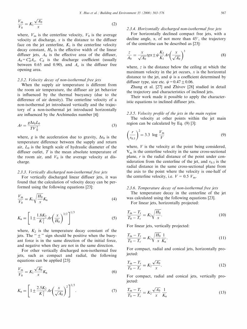
Vm

V0� K1

��A0

px

�2�

where, Vm is the centerline velocity, V0 is the averagevelocity at discharge, x is the distance to the di�userface on the jet centerline, K1 is the centerline velocitydecay constant, H0 is the e�ective width of the lineardi�user jets, A0 is the e�ective area of the di�user,A0=Cd

�Ac, Cd is the discharge coe�cient (usuallybetween 0.65 and 0.90), and Ac is the di�user freeopening area.

2.3.2. Velocity decay of non-isothermal free jetsWhen the supply air temperature is di�erent from

the room air temperature, the di�user air jet behavioris in¯uenced by the thermal buoyancy (due to thedi�erence of air density). The centerline velocity of anon-isothermal jet introduced vertically and the trajec-tory of a non-isothermal jet introduced horizontallyare in¯uenced by the Archimedes number [4]:

Ar � gDt0L0

TV 20

�3�

where, g is the acceleration due to gravity, Dt0 is thetemperature di�erence between the supply and returnair, L0 is the length scale of hydraulic diameter of thedi�user outlet, T is the mean absolute temperature ofthe room air, and V0 is the average velocity at dis-charge.

2.3.3. Vertically discharged non-isothermal free jetsFor vertically discharged linear di�user jets, it was

found that the calculation of velocity decay can be per-formed using the following equations [23]:

Vm

V0� K1

��H0

x

rKn �4�

Kn �"12

1:8K2

K 21

Ar

�x

H0

�3=2#1=3

�5�

where, K2 is the temperature decay constant of thejets. The ``2 '' sign should be positive when the buoy-ant force is in the same direction of the initial force,and negative when they are not in the same direction.

For other vertically discharged non-isothermal freejets, such as compact and radial, the followingequations can be applied [23]:

Vm

V0� K1

��A0

px

Kn �6�

Kn �"12

2:5K2

K 21

Ar

�x��A0

p�2#1=3

: �7�

2.3.4. Horizontally discharged non-isothermal free jetsFor horizontally declined compact free jets, with a

decline angle, a, of not more than 458, the trajectoryof the centerline can be described as [23]:

z

A0� x��

A0

p tga2cK2

K1Ar

�x��A0

p�3

�8�

where, z is the distance below the ceiling at which themaximum velocity in the jet occurs, x is the horizontaldistance to the jet, and c is a coe�cient determined bydi�user type, size etc. c=0.4720.06.

Zhang et al. [27] and Zhivov [28] studied in detailthe trajectory and characteristics of inclined jets.

Their work made it possible to apply the character-istic equations to inclined di�user jets.

2.3.5. Velocity pro®le of the jets in the main regionThe velocity at other points within the jet main

region can be calculated by Eq. (9) [3]:�r

r0:5

�2

� 3:3 logVm

V�9�

where, V is the velocity at the point being considered,Vm is the centerline velocity in the same cross-sectionalplane, r is the radial distance of the point under con-sideration from the centerline of the jet, and r0.5 is theradial distance in the same cross-sectional plane fromthe axis to the point where the velocity is one-half ofthe centerline velocity, i.e. V=0.5 Vm.

2.3.6. Temperature decay of non-isothermal free jetsThe temperature decay in the centerline of the jet

was calculated using the following equations [23].For linear jets, horizontally projected:

Tm ÿ Tr

T0 ÿ Tr

� K2

��H0

x

r: �10�

For linear jets, vertically projected:

Tm ÿ Tr

T0 ÿ Tr

� K2

��H0

x

r1

Kn

: �11�

For compact, radial and conical jets, horizontally pro-jected:

Tm ÿ Tr

T0 ÿ Tr

� K2

��A0

px: �12�

For compact, radial and conical jets, vertically pro-jected:

Tm ÿ Tr

T0 ÿ Tr

� K2

��A0

px

1

Kn

�13�


where, T0 is the supply temperature at the di�user, Tr

is the return air temperature, Tm is the temperaturealong the centerline of the jet main region, and K2 isthe temperature decay constant. Kn is a coe�cient cal-culated using Eqs. 5 and 7.

2.3.7. Temperature pro®le in the jet main regionThe relation between the velocity distribution and

temperature distribution in the cross section of non-isothermal jets is expressed by [3]:�

r

r0:5

�2

� 4:7 logTm ÿ Tr

Tÿ Tr

�14�

where, T is the actual air temperature at the pointbeing considered, Tm is the centerline air temperaturein the same cross-sectional plane, and Tr is the returnair temperature.

2.3.8. E�ects of ceilings and wallsJets discharge parallel to a surface with one edge of

the outlet coinciding with the surface take the form ofone-half of an axial jet discharging from an outlettwice as large, similar to radial jets from ceiling pla-ques. Entrainment takes place almost only along thesurface of a half cone, and the maximum velocityremains close to the surface [3].

Ceiling jets were found to attach to the ceiling and¯ow along it due to the ``Coanda'' e�ect if the initialjet axis was close to the ceiling [25]. The spread of thejet in the traversing direction was reduced when theaxis of a long jet was too close to the ceiling and par-allel to it. The angle of divergence of the jet awayfrom the wall was slightly less than one-half the angleof a free conical jet [25].

It was found that if an edge of the nozzle was incontact with the plane, as long as the axis of the noz-zle formed an angle less than 408±458 with the plane,the jet would cling to the plane and spread over it.However, if the edge of the jet was shifted away fromthe plane, air entrainment would occur on all sides ofthe jet, and the jet did not cling anymore [4]. If the jetattached to a ceiling or a wall, K1 became larger thanfree jets. The values of K1 were those of the free jetsmultiplied by 1.4 [3]. When the temperature of theattached air jet is lower than the temperature of theambient air, this jet will remain attached to the ceilinguntil the downward buoyancy force becomes greaterthan the upward static pressure (``Coanda'' force).

2.3.9. E�ect of con®nementThe con®ned centerline velocity Vmc and the tem-

perature di�erential Dtmc caused by the reverse ¯ow inthe room can be modi®ed using the coe�cient Kc [11]:

Vmc � Vm � Kc �15�

Dtmc � Dtm � 1

Kc

�16�

Where Vm is the centerline velocity calculated fromEqs. 1, 2, 4 or 6, and Dtm is the temperature di�erencebetween the jet centerline and the occupied region cal-culated from Eqs. 10±12 or 13. The values of Kc areavailable from graphs [11].

2.4. Di�user characteristic equation application

All these above equations are developed for themain region of the di�user jet. Since the ®rst tworegions are very small, the beginning of the mainregion is still close to the jet surface compared to theroom size. The parameters such as the e�ective supplyarea A0 and the average air supply velocity u0 can beobtained from the di�user's manufacturer product in-formation data. The velocity and temperature decaycoe�cient K1 and K2 for di�erent di�users are given inASHRAE Fundamentals. As long as the supply air-¯ow rate and the supply air temperature are given, thevelocity and temperature in the jet main region can becalculated using the di�user jet characteristicequations.

2.5. The new proposed di�user speci®cation method

The newly proposed di�user boundary conditionsspeci®cation method is a jet main region speci®cationmethod. It takes advantage of the existing di�usercharacteristic equations. The speci®cation of the com-plicated di�user boundary is transferred to the speci®-cation of the surfaces of a volume around the di�user.One volume surface is located inside the main regionof the di�user jet [16].

Fig. 3 shows the boundary conditions considered forthe di�user using the new proposed method. A two-dimensional air jet (linear air jets can be consideredtwo-dimensional) is applied in this ®gure. The air isintroduced into the room at an angle a to the verticaldirection. A1B1 is the jet opening. O1 is the center ofthe jet opening and O1O2 is the centerline of the sup-plying jet. A1A2 and B1B2 are the jet region borders.B2 is selected such that it is located at the beginning ofthe jet main region. A2 is chosen to make A2B2 paral-lel to the ceiling. Points C and D are selected to makeCA2DB1 a rectangular volume.

Point B2 dictates the height of the volume andpoints B1 and A2 specify the width of the volume. Aslong as A2B2 is located inside the jet main region, thevolume should be selected as small as possible to mini-mize the inaccuracy caused by the simpli®cation.

For three-dimensional di�users (radial, compactetc.), the volume can be selected in a similar manner.The approach is that, part of the volume surfaces need


to be located at the beginning of the jet main regionand the other part of the volume surfaces should beselected to make the volume as small as possible. Thiswill reduce the inaccuracy of the simpli®cation.

The uniqueness of the volume selection is that thejet main region concept is introduced and applied. Thesurfaces of the volume around the di�user are dividedinto two parts, inside the jet main region (A2B2) andoutside the jet main region (CA2, B2D and B1D), forthe boundary conditions speci®cation. One surface ofthe volume (A2D) could be partly inside the jet regionand partly outside the jet region (Fig. 3).

2.5.1. Boundary conditions of the selected volume

2.5.1.1. Velocity boundary conditions. The velocityboundary conditions of the volume surface inside thejet main region will be calculated using the jet mainregion characteristic equations.

For two-dimensional cases, as shown in Fig. 3, thevelocity components, temperature, k and E must bede®ned at the boundary. The velocity on the bound-ary, such as point E on line A2B2 (inside the jet mainregion), is obtained by determining the velocity of itsorthogonal projection point, OE, on the centerlineusing the velocity decay equations (Eqs. 1, 2 or 4). Theaverage velocity at discharge, V0, is obtained based onthe supply conditions and the di�user data from man-ufacturer's catalogue.

The velocity VE, then is calculated using the velocitypro®le equations based on the centerline velocity atpoint OE using Eq. 9. The velocity direction for thepoints on A2B2 is considered the same as the velocitydirection of the centerline since the velocity componentperpendicular to the centerline is very small compared

with the velocity component parallel to the centerline[4].

For the three dimensional cases, the velocity on thesurface located inside the jet main region can be calcu-lated in a similar manner. When the velocity of a pointon that surface, V, is needed, the velocity of its orthog-onal projection point on the centerline, Vm, is calcu-lated ®rst using Eqs. 2 or 6. Then the velocity, u, canbe calculated using Eq. 9. The distance, r, should be athree dimensional distance in Eq. 9.

When considering the boundary conditions of theother part of the volume surfaces, a zero gradient isassumed based on the fact that the velocity outside thejet main region does not have big changes [21]. Thevelocity component parallel to the volume surfaces isassumed as:

@V

@n� 0 �17�

where, n is the direction perpendicular to the volumesurface; and V is the velocity component parallel tothe volume surface. The velocity component perpen-dicular to the volume surface is determined by usingthe continuity equation in the simulation. Fig. 3 showsthe equations for a two dimensional case. The velocityof a three dimensional case can be similarly derived.

2.5.1.2. Temperature boundary conditions. Like the vel-ocity boundary conditions, the temperature boundaryconditions are also decided depending on whether thesurface of the volume is located inside or outside thejet main region.

The jet main region temperature characteristicequations are used for the temperature boundary con-ditions of the volume surface inside the jet main

Fig. 3. Boundary conditions in the jet main region.


region. The temperature on the di�user centerline iscalculated ®rst according to the supply air temperatureand the di�user type. When the temperature at a pointon the surface inside the jet main region, T, is needed,the temperature of that point's orthogonal projectionon the centerline, Tm, is calculated ®rst using Eqs. 10±12 or 13, depending on the di�user type. Then thetemperature at the point, T, can be calculated usingthe temperature pro®le (Eq. 14).

Zero temperature gradient is also assumed for thetemperature boundary conditions of the volume sur-faces outside the jet main region; considering that thetemperature variation between the inside and outsidejet main region is negligible.

@y@n� 0 �18�

where, y is the temperature di�erence, and n is thedirection perpendicular to the volume surface.

2.5.1.3. Boundary conditions for k and EE. The k and Eboundary conditions for the volume surface inside thejet region can be determined based on Rodi and Spald-ing's [20] work. For the same type of di�users, thesame dimensionless curve can be obtained in the jetmain region. They also suggested that E could be calcu-lated using the following equation:

E � CDk3=2

L�19�

where, CD is a constant, equal to 0.09 for a plane jetand 0.06 for a round jet; L is a length scale. Its valueapproximately equals to 0.075 d for a radial jet, 0.052 dfor a plane jet and 0.033 d for a round jet [22]. d is thedistance from the jet centerline to the edge of the jetregion at the location where E is speci®ed.

The boundary conditions, k and E, for the other partof the volume surfaces are described in a similar man-ner as the velocity and temperature boundary con-ditions. They are assumed as:

@k

@n� 0,

@E@n� 0 �20�

where, n is the direction perpendicular to the volumesurface, as shown in Fig. 3.

3. Validation of the proposed method

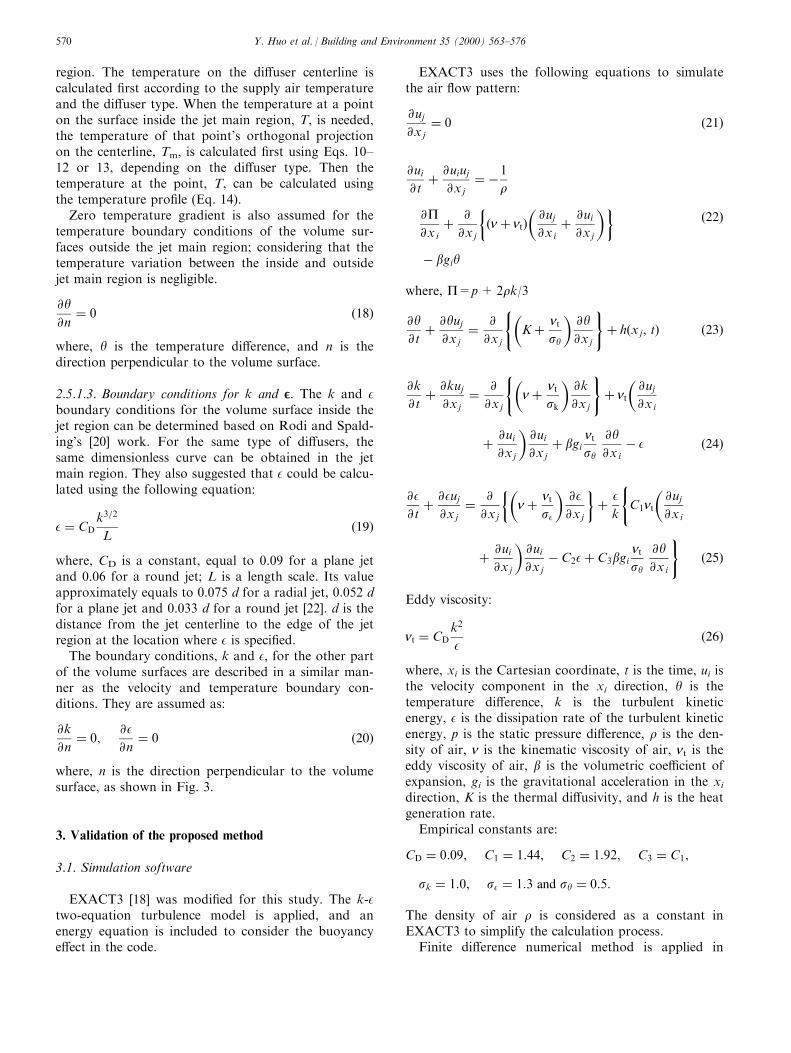
3.1. Simulation software

EXACT3 [18] was modi®ed for this study. The k-Etwo-equation turbulence model is applied, and anenergy equation is included to consider the buoyancye�ect in the code.

EXACT3 uses the following equations to simulatethe air ¯ow pattern:

@uj@xj� 0 �21�

@ui@t� @uiuj@xj� ÿ1

r

@P@xi� @

@xj

��n� nt�

�@uj@xi� @ui@xj

��ÿ bgiy

�22�

where, P=p+2rk/3

@y@t� @yuj@xj� @

@xj

(�K� nt

sy

�@y@xj

)� h�xj, t� �23�

@k

@ t� @kuj@xj� @

@xj

(�n� nt

sk

�@k

@xj

)� nt

�@uj@xi

� @ui@xj

�@ui@xj� bgi

nt

sy

@y@xiÿ E �24�

@E@ t� @Euj@xj� @

@xj

��n� nt

sE

�@E@xj

�� E

k

(C1nt

�@uj@xi

� @ui@xj

�@ui@xjÿ C2E� C3bgi

nt

sy

@y@xi

)�25�

Eddy viscosity:

nt � CDk2

E�26�

where, xi is the Cartesian coordinate, t is the time, ui isthe velocity component in the xi direction, y is thetemperature di�erence, k is the turbulent kineticenergy, E is the dissipation rate of the turbulent kineticenergy, p is the static pressure di�erence, r is the den-sity of air, n is the kinematic viscosity of air, nt is theeddy viscosity of air, b is the volumetric coe�cient ofexpansion, gi is the gravitational acceleration in the xidirection, K is the thermal di�usivity, and h is the heatgeneration rate.

Empirical constants are:

CD � 0:09, C1 � 1:44, C2 � 1:92, C3 � C1,

sk � 1:0, sE � 1:3 and sy � 0:5:

The density of air r is considered as a constant inEXACT3 to simplify the calculation process.

Finite di�erence numerical method is applied in


EXACT3, and the ``Marker and Cell'' (MAC) methodis implemented to solve these equations [18]. A pseudotime step is used and the simulation reaches a steadystate result when the accumulated time step converges.

EXACT3 can only be used to simulate a rectangularregion. To apply the new di�user description method,the boundary condition subroutine of the EXACT3code was modi®ed to assign the boundary conditionsof the volume around the di�user.

3.2. Case studies

Three cases were studied to verify the validity of thenew proposed jet main region speci®cation method fordi�user boundary conditions description in CFD simu-lation. The ®rst two cases were designed to validatewhether the new method is applicable and whether thenew method can improve the prediction and conver-gence. The third case was designed to compare the per-formance of the new method with the experimentalresults and with the prediction of conventionalmethod.

3.2.1. First caseIn the ®rst case, a simple linear di�user under a two

dimensional isothermal condition was studied. Sincethe conventional method provides correct predictions

for simple geometry di�users, such as the one appliedin this case, the prediction of the conventional method

was treated as a correct solution.

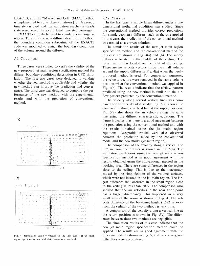
The simulation results of the new jet main region

speci®cation method and the conventional method forthis case are shown in Fig. 4(a) and (b). The supply

di�user is located in the middle of the ceiling. Thereturn air grill is located on the right of the ceiling.

There are no velocity vectors inside the small volumearound the supply di�user in Fig. 4(a) when the newly

proposed method is used. For comparison purposes,the velocity vectors were removed in the same volume

position when the conventional method was applied inFig. 4(b). The results indicate that the air¯ow pattern

predicted using the new method is similar to the air-¯ow pattern predicted by the conventional method.

The velocity along several vertical lines was com-pared for further detailed study. Fig. 5(a) shows the

comparison along a vertical line at the supply position.Fig. 5(a) also shows the air velocity along the same

line using the di�user characteristic equations. The®gure indicates that there is a good agreement between

the prediction using the conventional method and withthe results obtained using the jet main region

equations. Acceptable results were also observedbetween the prediction made by the conventional

model and the new model (jet main region).

The comparison of the velocity along a vertical line0.75 m from the di�user is shown in Fig. 5(b). The

simulation predictions using the new jet main regionspeci®cation method is in good agreement with the

results obtained using the conventional method in the

working area. There are some di�erences in the regionclose to the ceiling. This is due to the inaccuracy

caused by the simpli®cation of the volume surfaces,which were not located in the jet main region. The lar-

gest di�erence that occurred in the small region closeto the ceiling is less than 20%. The comparison also

showed that the air velocities in the near ¯oor pointhas a bigger discrepancy. This happened in a very

small area of the room as shown in Fig. 4. The vel-ocity di�erence at the breathing height (1.5±2 m away

from the ceiling) of the two methods is very little.

A comparison of the velocity along a vertical line atthe return position is shown in Fig. 5(c). The di�er-

ences between these two methods are negligible.

The simulation results of this case indicate that the

new jet main region speci®cation method could beapplied. The results are in good agreement with the

other methods as shown in Fig. 5, and no convergencedi�culties were encountered.

Fig. 4. Simulation velocity vectors in the ®rst case: (a) jet main

region speci®cation method; (b) conventional method.


3.2.2. Second caseThe second case was similar to the ®rst one and the

only di�erence was that the direction of the supply airwas not perpendicular to the ceiling but at an angle of608. In such a condition, there is di�culty in selectingthe volume around the di�user as well as setting theappropriate boundary conditions for the selectedvolume. If such a situation can be simulated correctly,we will know how to simulate supply di�users, whichsupply air neither horizontally or vertically. This casewas designed to examine whether the simpli®cationsunder this critical condition would cause any pro-blems. In this case, two and a half edges of the volume

were located outside the jet main region. Simpli®cationof the boundary conditions had to be applied to allthese edges. Furthermore, the simpli®cations wereapplied to more than one direction. The boundaryconditions of two edges perpendicular to the ceilingand one edge parallel to the ceiling all needed to besimpli®ed. In the simpli®ed part of the volume bound-aries, the air may move out the volume in one positionand move into the volume in another position (seeFig. 3). In short, many more simpli®cations wererequired for this case.

The velocity vector distribution of the simulationusing the new jet main region speci®cation method is

Fig. 5. Detailed velocity comparison of the ®rst case: (a) air velocity in a vertical line (supply position); (b) air velocity in a vertical line (0.75 m

from the supply); (c) air velocity in a vertical line (return position).


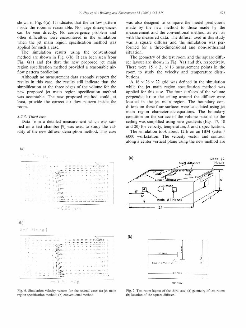
shown in Fig. 6(a). It indicates that the air¯ow patterninside the room is reasonable. No large discrepanciescan be seen directly. No convergence problem andother di�culties were encountered in the simulationwhen the jet main region speci®cation method wasapplied for such a case.

The simulation results using the conventionalmethod are shown in Fig. 6(b). It can been seen fromFig. 6(a) and (b) that the new proposed jet mainregion speci®cation method provided a reasonable air-¯ow pattern prediction.

Although no measurement data strongly support theresults in this case, the results still indicate that thesimpli®cation at the three edges of the volume for thenew proposed jet main region speci®cation methodwas acceptable. The new proposed method could, atleast, provide the correct air ¯ow pattern inside theroom.

3.2.3. Third caseData from a detailed measurement which was car-

ried on a test chamber [9] was used to study the val-idity of the new di�user description method. This case

was also designed to compare the model predictionsmade by the new method to those made by themeasurement and the conventional method, as well aswith the measured data. The di�user used in this studywas a square di�user and the simulation was per-formed for a three-dimensional and non-isothermalsituation.

The geometry of the test room and the square di�u-ser layout are shown in Fig. 7(a) and (b), respectively.There were 15 � 21 � 16 measurement points in theroom to study the velocity and temperature distri-butions.

A 16 � 26 � 22 grid was de®ned in the simulationwhile the jet main region speci®cation method wasapplied for this case. The four surfaces of the volumeperpendicular to the ceiling around the di�user werelocated in the jet main region. The boundary con-ditions on these four surfaces were calculated using jetmain region characteristic-equations. The boundarycondition on the surface of the volume parallel to theceiling was simpli®ed using zero gradients (Eqs. 17, 18and 20) for velocity, temperature, k and E speci®cation.

The simulation took about 12 h on an IBM system/6000 workstation. The velocity vector and contouralong a center vertical plane using the new method are

Fig. 7. Test room layout of the third case: (a) geometry of test room;

(b) location of the square di�user.

Fig. 6. Simulation velocity vectors for the second case: (a) jet main

region speci®cation method; (b) conventional method.


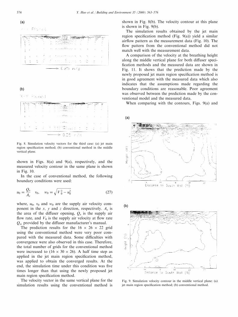
shown in Figs. 8(a) and 9(a), respectively, and themeasured velocity contour in the same plane is shownin Fig. 10.

In the case of conventional method, the followingboundary conditions were used:

u0 � Qs

Ac

v0, w0 ��V 2

0 ÿ u20

q�27�

where, u0, v0 and w0 are the supply air velocity com-ponent in the x, y and z direction, respectively. Ac isthe area of the di�user opening, Qs is the supply air¯ow rate, and V0 is the supply air velocity at ¯ow rateQs, provided by the di�user manufacturer's manual.

The prediction results for the 16 � 26 � 22 gridusing the conventional method were very poor com-pared with the measured data. Some di�culties withconvergence were also observed in this case. Therefore,the total number of grids for the conventional methodwere increased to (16 � 30 � 26). A half time step asapplied in the jet main region speci®cation method,was applied to obtain the converged results. At theend, the simulation time under this condition was ®vetimes longer than that using the newly proposed jetmain region speci®cation method.

The velocity vector in the same vertical plane for thesimulation results using the conventional method is

shown in Fig. 8(b). The velocity contour at this planeis shown in Fig. 9(b).

The simulation results obtained by the jet mainregion speci®cation method (Fig. 9(a)) yield a similarair¯ow pattern as the measurement data (Fig. 10). The¯ow pattern from the conventional method did notmatch well with the measurement data.

A comparison of the velocity at the breathing heightalong the middle vertical plane for both di�user speci-®cation methods and the measured data are shown inFig. 11. It shows that the prediction made by thenewly proposed jet main region speci®cation method isin good agreement with the measured data which alsoindicates that the assumptions made regarding theboundary conditions are reasonable. Poor agreementwas observed between the prediction made by the con-ventional model and the measured data.

When comparing with the contours, Figs. 9(a) and

Fig. 8. Simulation velocity vectors for the third case: (a) jet main

region speci®cation method; (b) conventional method in the middle

vertical plane.

Fig. 9. Simulation velocity contour in the middle vertical plane: (a)

jet main region speci®cation method; (b) conventional method.


10, air velocity di�erences between the newly proposedmethod and the measured data exist if the entire roomis considered. The air velocity in the jet main region,calculated using the jet characteristic equations was alittle higher than the measured data. This might causesome inaccuracy. It could be improved by developingmore accurate jet characteristic equations. In spite ofthis, the predicted results using the new jet main regionspeci®cation method was much better than the conven-tional method when compared to the measured data.

4. Conclusions

It can be concluded from the case studies that, thenewly proposed jet main region speci®cation methodhas proved to be an applicable approach and a more

accurate way to study the air¯ow pattern in a venti-

lated room.

The jet main region speci®cation method is devel-

oped based on the box method. However, they are not

the same. The main di�erences are as follows.

1. The use of the jet main region concept: the jet main

region speci®cation method applies the analytical

data only to the volume boundaries inside the jet

main region. The volume boundary could be fully

or partially located inside the jet main region. In

Nielson's box method [19], the boundary conditions

of the box use fully analytical data or fully

measured data.

2. The selection of the box: the jet main region speci®-

cation method accurately describes how to select a

volume around the di�user. The volume boundary

is accurately set after the di�user is located and its

jet main region is calculated. The original box

method did not specify how to improve the accu-

racy by selecting the box. Recently, Nielson [20]

suggested a procedure for selecting the box, result-

ing in a suggested range of possible selection rather

than a unique selection.

3. The ®tting for di�erent kinds of di�users and room

situations: the jet main region speci®cation method

can be applied conveniently to di�erent kind of dif-

fusers and room situations. For example, when the

air jet has an angle with the di�user, the volume

boundary can be partially located inside the jet

main region. Such a situation will be a problem in

the box method. There is no analytical data avail-

able on any side of the box.

The advantages of the newly proposed method are as

follows.

1. The user can avoid describing the complicated di�u-

ser geometry by using data from manufacturer's cat-

alogs.

2. It provides an accurate prediction of the air ¯ow

patterns in a ventilated room.

3. The method is applicable for di�erent di�users.

4. It reduces the simulation time appreciably since a

lower grid density is required.

It should also be noted that, when the new jet main

region speci®cation method is applied, it is very im-

portant to ®nd the suitable di�user characteristic

equations. Calculation is required for the jet main

region boundary conditions speci®cation.

Although the new method is not a perfect one, it

leads to a much better air¯ow pattern prediction in

air-conditioned rooms than the conventional method,

while a complicated geometry supply air di�user is

presented. This method can be enhanced with the

development of more accurate di�user characteristic

Fig. 10. Measurement velocity contour in the middle vertical plane.

Fig. 11. Detailed velocity comparison of the third case.


equations and the development of the CFD simulationsoftware.

Acknowledgements

Dr Zhenhai Li of the University of Illinois kindlyprovided the measured data. His support is highly ap-preciated

References

[1] Abramovich GN. The theory of turbulent jets. Moscow:

Fizmatgiz, 1960.

[2] Albright LD. Research needs. In: Christianson LL, editor.

Building system: room air and air contaminant distribution.

USA: ASHRAE, 1989. p. 8±10.

[3] ASHRAE Fundamentals. Space air di�usion. USA: ASHRAE,

1993 Chapter 31.

[4] Baturin VV. Fundamentals of industrial ventilation, 3rd ed.

New York: Pergamon Press, 1972.

[5] Chen Q, Moser A. Simulation of a multiple nozzle di�user. In:

Proceedings of the Twelfth AIVC Conference, Ottawa, Canada,

1991a. Vol. 2. p. 1±14.

[6] Chen Q, Suter P, Moser A. A database for assessing indoor air

¯ow, air quality and draught risk. ASHRAE Transactions

1991;97(2):150±63.

[7] Chen Q, Jiang Z. Evaluation of air supply method in a class-

room with a low ventilation rate. In: Proceedings of Indoor Air

Quality, Ventilation and Energy Conservation Conference,

Montreal, Canada, 1992. p. 412±9.

[8] Chen Q, Jiang Z. Simulation of a complex air di�user with

CFD technique. In: Fifth International Conference on Air

Distribution in Rooms, RoomVent'96, Yokohama, Japan, 1996.

Vol. 1. p. 227±34.

[9] Christianson LL et al. Low temperature air distribution: jet of

low temperature air, Final Report for ASHRAE Project ]]705,ASHRAE, USA, 1994.

[10] Emvin P, Davidson L. A numerical comparison of three inlet

approximations of the di�user in Case E1 Annex20. In: Fifth

International Conference on Air Distribution in Rooms,

RoomVent'96, Yokohama, Japan, 1996. Vol. 1. p. 219±26.

[11] Grimitlyn M, Pozin G. Determination of parameters for the jet

in a con®ned space following blocked or through ¯ow pattern.

In: Proceedings of Research Institutes for Labor Protection

VTsSPS 91, Moscow: Pro®zdat, 1973.

[12] Haghighat F, Jiang Z, Wang JCY. A CFD analysis of venti-

lation e�ectiveness in a partitioned room. Indoor Air

1991;1(3):606±15.

[13] Haghighat F, Jiang J, Zhang Y. The impact of ventilation rate

and partition layout on the VOC emission rate: time-dependent

contaminant removal. Indoor Air 1994;4:276±83.

[14] Haghighat F, Huo Y, Zhang J, Shaw CY. The in¯uence of

o�ce furniture, workstation layouts, di�user types and location

on indoor air quality and thermal comfort at workstations.

Indoor Air 1996;6:188±203.

[15] Heikkinen J. Modeling of a supply air terminal for room air

¯ow simulation. In: Twelfth AIVC Conference, Ottawa,

Canada, 1991. Vol. 3. p. 213±30.

[16] Huo Y, Zhang JS, Shaw CY, Haghighat F. A new method to

specify the di�user boundary conditions in CFD simulation. In:

Fifth International Conference on Air Distribution in Rooms,


[17] Jiang Z, Chen Q, Moser A. Comparison of displacement and

mixing di�users. Indoor Air 1992;2(3):168±79.

[18] Kurabuchi T, Fang JB, Rechard AG. A numerical method for

calculating indoor air ¯ows using a turbulence model, US

Department of Commerce, NISTIR 89-4211, 1989.

[19] Nielsen PV. Description of supply openings in numerical models

for room air distribution. ASHRAE Transaction

1992;98(1):963±71.

[20] Nielsen PV. The box Method Ð a Practical procedure for intro-

duction of an air terminal device in CFD calculation, Institute

for Bygningsteknik, Aaborg University, Denmark, 1997.

[21] Nielsen PV, Restivo A, Whitelaw JH. The velocity character-

istics of ventilated rooms. Journal of Fluid Engineering

1978;100:291±8.

[22] Rodi W, Spalding DB. A two-parameter model of turbulence

and its application to free jets. In: Numerical prediction of ¯ow,

heat transfer, turbulence, and combustion: selected works of

Professor D. Brian Spalding. Oxford; New York: Pergamon

Press, 1983. p. 22±32.

[23] Shepelev I. Air supply ventilation jets and air fountains. In:

Proceedings of the Academy of Construction and Architecture

of the USSR 4, Moscow, 1961.

[24] Skovgaard M, Nielsen PV. Modeling complex inlet geometry in

CFD ± applied to air ¯ow in ventilated rooms. In: Proceedings

of the Twelfth AIVC Conference, Ottawa, Canada, 1991. Vol.

3. p. 183±200.

[25] Tuve GL. Air velocity in ventilating jets, ASHRAE researches

report No. 1467, ASHRAE Transaction Vol. 59, p. 261, 1953.

[26] Zhang JS, Christianson LL, Wu GJ, Zhang RH. An experimen-

tal evaluation of a numerical simulation model for prediction

room air motion. In: Proceedings of Indoor Air Quality,

Ventilation and Energy Conservation Conference, Montreal,

Canada, 1992. p. 360±71.

[27] Zhang G, Strom JS, Morsing S. Jet drop models for control of

cold air jet trajectories in ventilated livestock buildings. In:

Fifth International Conference on Air Distribution in Rooms,


[28] Zhivov A. Theory and practice of air distribution with inclined

jets. ASHRAE Transaction 1993;99(1):1152±9.


1-s2.0-S0360132399000475-main

Documents

features of air

room air velocity

ventilated room

theindoor air quality

supply air flowcondition

contaminant distribution

conventional method

cfd method hasbeen