1 RL for Large State Spaces: Value Function Approximation Alan Fern * Based in part on slides by Daniel Weld.

1

RL for Large State Spaces: Value Function Approximation

Alan Fern

* Based in part on slides by Daniel Weld

2

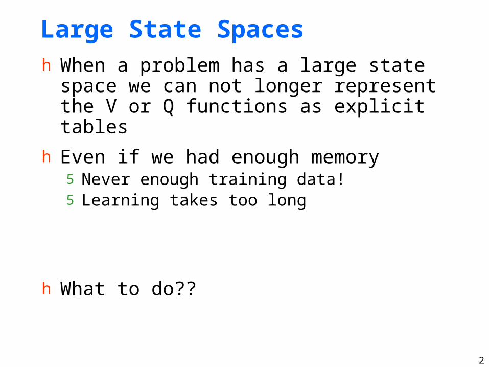
Large State Spacesh When a problem has a large state space we

can not longer represent the V or Q functions as explicit tables

h Even if we had enough memory 5 Never enough training data!5 Learning takes too long

h What to do??

3

Function Approximation

h Never enough training data!5 Must generalize what is learned from one situation to other

“similar” new situations

h Idea: 5 Instead of using large table to represent V or Q, use a

parameterized functiong The number of parameters should be small compared to

number of states (generally exponentially fewer parameters)

5 Learn parameters from experience5 When we update the parameters based on observations in

one state, then our V or Q estimate will also change for other similar states

g I.e. the parameterization facilitates generalization of experience

4

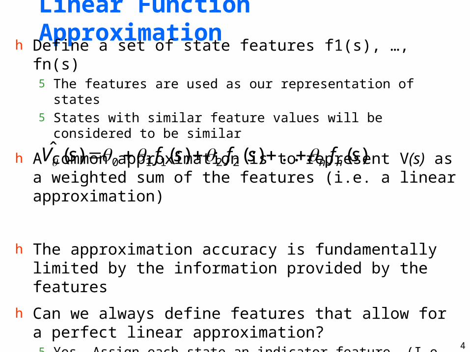
Linear Function Approximationh Define a set of state features f1(s), …, fn(s)

5 The features are used as our representation of states5 States with similar feature values will be considered to be similar

h A common approximation is to represent V(s) as a weighted sum of the features (i.e. a linear approximation)

h The approximation accuracy is fundamentally limited by the information provided by the features

h Can we always define features that allow for a perfect linear approximation?5 Yes. Assign each state an indicator feature. (I.e. i’th feature is 1 iff i’th

state is present and i represents value of i’th state)

5 Of course this requires far too many features and gives no generalization.

)(...)()()(ˆ 22110 sfsfsfsV nn

5

Exampleh Grid with no obstacles, deterministic actions U/D/L/R, no

discounting, -1 reward everywhere except +10 at goalh Features for state s=(x,y): f1(s)=x, f2(s)=y (just 2 features)h V(s) = 0 + 1 x + 2 yh Is there a good linear

approximation?5 Yes. 5 0 =10, 1 = -1, 2 = -15 (note upper right is origin)

h V(s) = 10 - x - ysubtracts Manhattan dist.from goal reward

10

0

0

6

6

6

But What If We Change Reward …

h V(s) = 0 + 1 x + 2 y

h Is there a good linear approximation?5 No.

10

0

0

7

But What If…

h V(s) = 0 + 1 x + 2 y

10

+ 3 z

h Include new feature z5 z= |3-x| + |3-y|

5 z is dist. to goal location

h Does this allow a

good linear approx?

5 0 =10, 1 = 2 = 0,

3 = -1

0

0

3

3

8

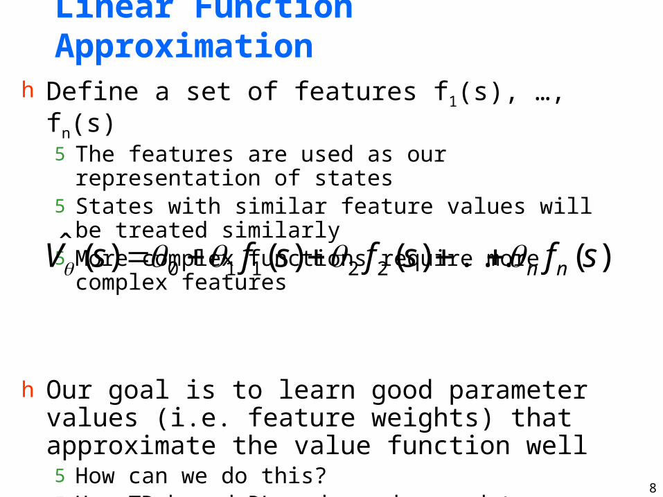
Linear Function Approximation

h Define a set of features f1(s), …, fn(s)5 The features are used as our representation of states5 States with similar feature values will be treated

similarly5 More complex functions require more complex features

h Our goal is to learn good parameter values (i.e. feature weights) that approximate the value function well5 How can we do this?5 Use TD-based RL and somehow update parameters

based on each experience.

)(...)()()(ˆ 22110 sfsfsfsV nn

9

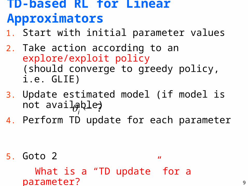
TD-based RL for Linear Approximators

1. Start with initial parameter values

2. Take action according to an explore/exploit policy(should converge to greedy policy, i.e. GLIE)

3. Update estimated model (if model is not available)

4. Perform TD update for each parameter

5. Goto 2

What is a “TD update” for a parameter?

?i

10

Aside: Gradient Descenth Given a function E(1,…, n) of n real values =(1,…, n) suppose

we want to minimize E with respect to

h A common approach to doing this is gradient descent

h The gradient of E at point , denoted by E(), is an n-dimensional vector that points in the direction where f increases most steeply at point

h Vector calculus tells us that E() is just a vector of partial derivatives

where

h Decrease E by moving in negative gradient direction

)(),,,,,(lim

)( 111

0

EEE niii

i

n

EEE

)(,,

)()(

1

11

Aside: Gradient Descent for Squared Error

h Suppose that we have a sequence of states and target values for each state5 E.g. produced by the TD-based RL loop

h Our goal is to minimize the sum of squared errors between our estimated function and each target value:

h After seeing j’th state the gradient descent rule tells us that we can decrease error wrt by updating parameters by:

2)()(ˆ2

1)( jjj svsVE

squared error of example j our estimated valuefor j’th state

learning rate

target value for j’th state

,)(,,)(, 2211 svssvs

i

jii

E

12

Aside: continued

i

j

j

ji

i

jii

sV

sV

EE

)(ˆ

)(ˆ

• For a linear approximation function:

• Thus the update becomes:

• For linear functions this update is guaranteed to converge to best approximation for suitable learning rate schedule

)(...)()()(ˆ 22111 sfsfsfsV nn

)()(ˆ)( jijjii sfsVsv

)()(ˆ

jii

j sfsV

depends on form of approximator

2)()(ˆ2

1)( jjj svsVE )

13

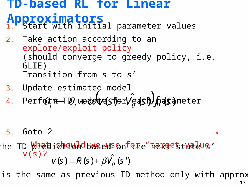
TD-based RL for Linear Approximators1. Start with initial parameter values

2. Take action according to an explore/exploit policy (should converge to greedy policy, i.e. GLIE) Transition from s to s’

3. Update estimated model

4. Perform TD update for each parameter

5. Goto 2

What should we use for “target value” v(s)?

)()(ˆ)( sfsVsv iii

• Use the TD prediction based on the next state s’

this is the same as previous TD method only with approximation

)'(ˆ)()( sVsRsv

14

TD-based RL for Linear Approximators1. Start with initial parameter values

2. Take action according to an explore/exploit policy(should converge to greedy policy, i.e. GLIE)

3. Update estimated model

4. Perform TD update for each parameter

5. Goto 2

)()(ˆ)'(ˆ)( sfsVsVsR iii

• Step 2 requires a model to select greedy action

• For some applications (e.g. Backgammon ) it is easy to get a compact model representation (but not easy to get policy), so TD is appropriate.

• For others it is difficult to small/compact model representation

15

Q-function Approximation

h Define a set of features over state-action pairs: f1(s,a), …, fn(s,a)5 State-action pairs with similar feature values will be

treated similarly5 More complex functions require more complex features

h Just as for TD, we can generalize Q-learning to update the parameters of the Q-function approximation

),(...),(),(),(ˆ 22110 asfasfasfasQ nn Features are a function of states and actions.

16

Q-learning with Linear Approximators

1. Start with initial parameter values

2. Take action a according to an explore/exploit policy(should converge to greedy policy, i.e. GLIE) transitioning from s to s’

3. Perform TD update for each parameter

4. Goto 2

),(),(ˆ)','(ˆmax)('

asfasQasQsR ia

ii

• TD converges close to minimum error solution

• Q-learning can diverge. Converges under some conditions.

estimate of Q(s,a) based on observed transition

17

Defining State-Action Featuresh Often it is straightforward to define features of

state-action pairs (example to come)

h In other cases it is easier and more natural to define features on states f1(s), …, fn(s)5 Fortunately there is a generic way of deriving state-

features from a set of state features

h We construct a set of n x |A| state-action features

otherwise

aaifsfasf ki

ik ,0

),(),( |}|,..,1{},,..,1{ Akni

18

Defining State-Action Featuresh This effectively replicates the state features

across actions, and activates only one set of features based on which action is selected

h h Each action has its own set of parameters

19

20

Example: Tactical Battles in Wargus

h Wargus is real-time strategy (RTS) game5 Tactical battles are a key aspect of the game

h RL Task: learn a policy to control n friendly agents in a battle against m enemy agents5 Policy should be applicable to tasks with different sets and

numbers of agents

5 vs. 5 10 vs. 10

21

Example: Tactical Battles in Wargus

h States: contain information about the locations, health, and current activity of all friendly and enemy agents

h Actions: Attack(F,E) 5 causes friendly agent F to attack enemy E

h Policy: represented via Q-function Q(s,Attack(F,E))5 Each decision cycle loop through each friendly agent F and select

enemy E to attack that maximizes Q(s,Attack(F,E))

h Q(s,Attack(F,E)) generalizes over any friendly and enemy agents F and E5 We used a linear function approximator with Q-learning

h RL Task: learn a policy to control n friendly agents in a battle against m enemy agents5 Policy should be applicable to tasks with different sets and numbers of

agents5 That is, policy should be relational

22

Example: Tactical Battles in Wargus

h Engineered a set of relational features {f1(s,Attack(F,E)), …., fn(s,Attack(F,E))}

h Example Features: 5 # of other friendly agents that are currently attacking E5 Health of friendly agent F5 Health of enemy agent E5 Difference in health values5 Walking distance between F and E5 Is E the enemy agent that F is currently attacking?5 Is F the closest friendly agent to E? 5 Is E the closest enemy agent to E? 5 …

h Features are well defined for any number of agents

),(...),(),(),(ˆ 22111 asfasfasfasQ nn

23

Example: Tactical Battles in Wargus

Initial random policy

24

Example: Tactical Battles in Wargush Linear Q-learning in 5 vs. 5 battle

-100

0

100

200

300

400

500

600

700

Dam

age

Diffe

rent

ial

Episodes

25

Example: Tactical Battles in Wargus

Learned Policy after 120 battles

26

Example: Tactical Battles in Wargus

10 vs. 10 using policy learned on 5 vs. 5

27

Example: Tactical Battles in Wargush Initialize Q-function for 10 vs. 10 to one learned

for 5 vs. 55 Initial performance is very good which demonstrates

generalization from 5 vs. 5 to 10 vs. 10

28

Q-learning w/ Non-linear Approximators

1. Start with initial parameter values

2. Take action according to an explore/exploit policy(should converge to greedy policy, i.e. GLIE)

3. Perform TD update for each parameter

4. Goto 2

i

aii

asQasQasQsR

),(ˆ

),(ˆ)','(ˆmax)('

),(ˆ asQ

• Typically the space has many local minima and we no longer guarantee convergence

• Often works well in practice

is sometimes represented by a non-linearapproximator such as a neural network

calculate closed-form

29

~Worlds Best Backgammon Player

h Neural network with 80 hidden units

h Used TD-updates for 300,000 games of self-play

h One of the top (2 or 3) players in the world!