1 Review – Biological Neuron The Neuron - A Biological Information Processor dentrites - the receivers soma - neuron cell body (sums input signals) axon.

1

Review – Biological NeuronReview – Biological Neuron

The Neuron - A Biological Information Processor• dentrites - the receivers• soma - neuron cell body (sums input signals)• axon - the transmitter• synapse - point of transmission• neuron activates after a certain threshold is met

Learning occurs via electro-chemical changes in effectiveness of synaptic junction.

2

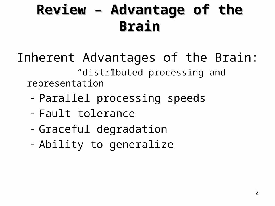
Review – Advantage of the BrainReview – Advantage of the Brain

Inherent Advantages of the Brain: “distributed processing and representation”

– Parallel processing speeds– Fault tolerance– Graceful degradation– Ability to generalize

3

OUTLINE

• Features of Neural Nets

• Learning in Neural Nets

• McCulloch/Pitts Neuron

• Hebbian Learning

4

Features of Neural Nets Neural Net Characteristics 1

• Neural nets have many unique features:

Massive Parallel Processing:

Computers calculate in sequenceNeural Nets update in parallel

5

Neural Net Characteristics 2

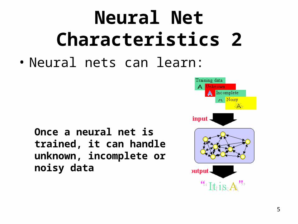
• Neural nets can learn:

Once a neural net is trained, it can handle unknown, incomplete or noisy data

6

Neural Net Characteristics 3

• Unlike computer memory, information is distributed over the entire network, so a failure in one part of the network does not prevent the system for producing the correct output.

7

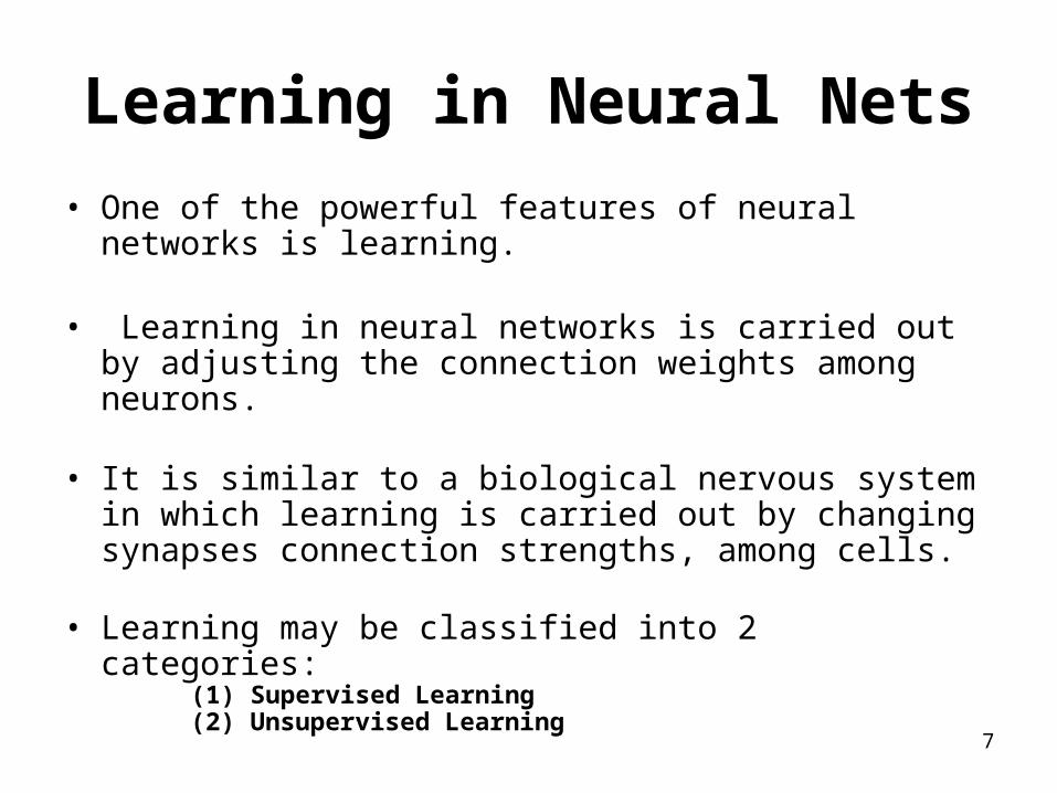
Learning in Neural Nets

• One of the powerful features of neural networks is learning.

• Learning in neural networks is carried out by adjusting the connection weights among neurons.

• It is similar to a biological nervous system in which learning is carried out by changing synapses connection strengths, among cells.

• Learning may be classified into 2 categories: (1) Supervised Learning (2) Unsupervised Learning

8

OUTLINE

• Introduction to Learning

• Learning Methods

• Introduction to Learning by Induction

9

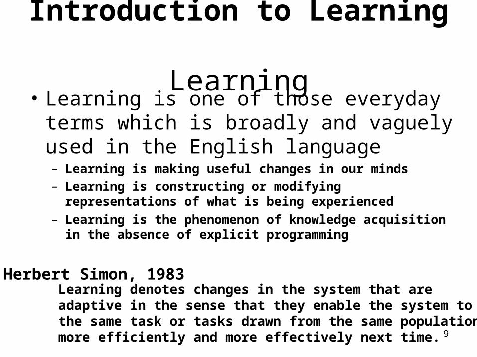
Introduction to Learning Learning

• Learning is one of those everyday terms which is broadly and vaguely used in the English language– Learning is making useful changes in our minds

– Learning is constructing or modifying representations of what is being experienced

– Learning is the phenomenon of knowledge acquisition in the absence of explicit programming

Herbert Simon, 1983Learning denotes changes in the system that areadaptive in the sense that they enable the system to dothe same task or tasks drawn from the same populationmore efficiently and more effectively next time.

10

Learning is . . .

• Learning involves the recognition of patterns in data or experience and then using that information to improve performance on another task

11

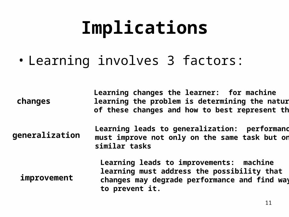
Implications

• Learning involves 3 factors:

changes

generalization

improvement

Learning changes the learner: for machinelearning the problem is determining the natureof these changes and how to best represent them

Learning leads to generalization: performancemust improve not only on the same task but on similar tasks

Learning leads to improvements: machine learning must address the possibility that changes may degrade performance and find waysto prevent it.

12

Learning Methods

• There are two different kinds of information processing which must be considered in a machine learning system– Inductive learning is concerned with determining

general patterns, organizational schemes, rules, and laws from raw data, experience or examples.

– Deductive learning is concerned with determination of specific facts using general rules or the determination of new general rules from old general rules.

13

Learning Framework

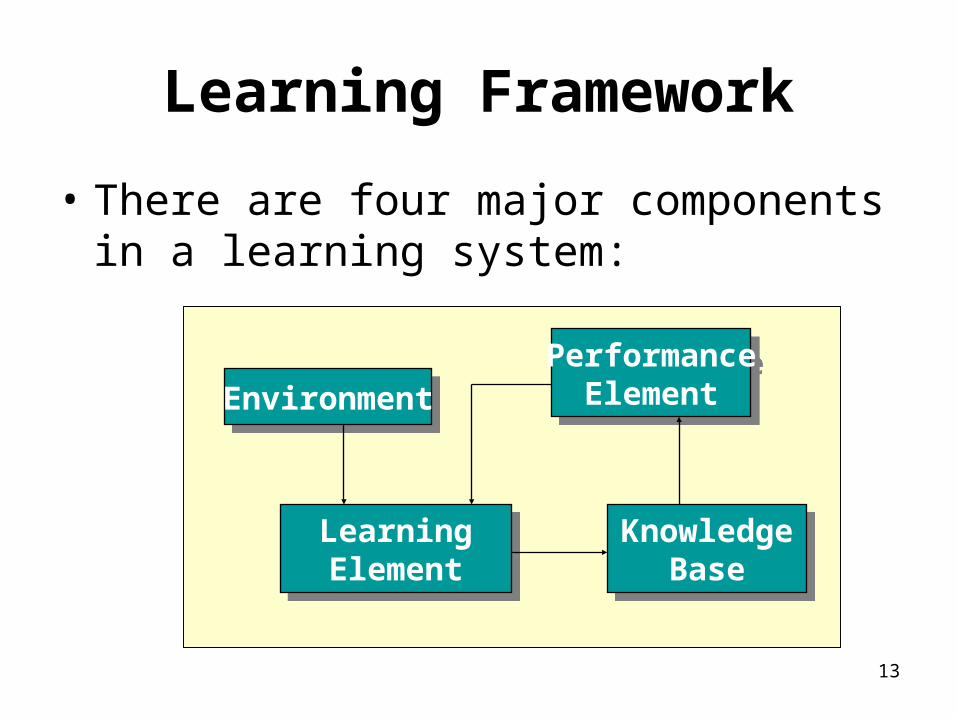
• There are four major components in a learning system:

EnvironmentEnvironment

LearningElement

LearningElement

PerformanceElement

PerformanceElement

KnowledgeBase

KnowledgeBase

14

The Environment

• The environment refers the nature and quality of information given to the learning element

• The nature of information depends on its level (the degree of generality wrt the performance element)– high level information is abstract, it deals with a broad class of

problems– low level information is detailed, it deals with a single problem.

• The quality of information involves– noise free– reliable– ordered

15

Learning Elements

• Four learning situations– Rote Learning

• environment provides information at the required level

– Learning by being told• information is too abstract, the learning element must

hypothesize missing data

– Learning by example• information is too specific, the learning element must

hypothesize more general rules

– Learning by analogy• information provided is relevant only to an analogous task,

the learning element must discover the analogy

16

Knowledge Base

• Expressive– the representation contains the relevant knowledge in

an easy to get to fashion

• Modifiable– it must be easy to change the data in the knowledge

base

• Extendibility– the knowledge base must contain meta-knowledge

(knowledge on how the data base is structured) so the system can change its structure

17

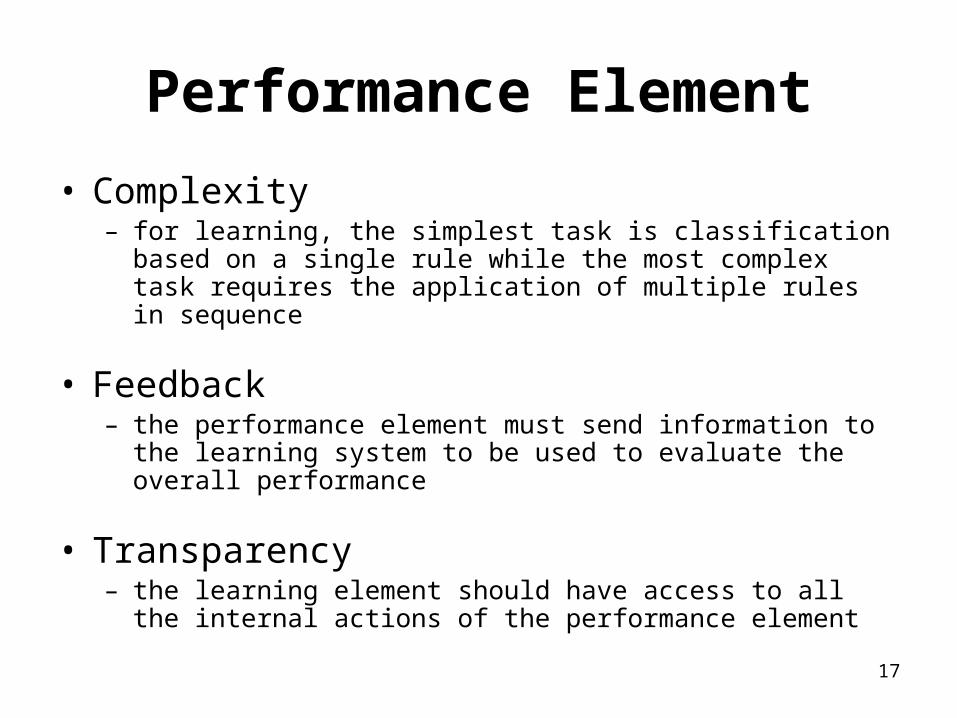
Performance Element

• Complexity– for learning, the simplest task is classification based on a single

rule while the most complex task requires the application of multiple rules in sequence

• Feedback– the performance element must send information to the learning

system to be used to evaluate the overall performance

• Transparency– the learning element should have access to all the internal

actions of the performance element

18

Rote Learning

• Memorization - saving new knowledge to be retrieved when needed rather than calculated

• Works by taking problems that the performance element has solved and memorizing the problem and the solution

• Only useful if it takes less time to retrieve the knowledge than it does to recompute it

19

Checkers Example

• A.L. Samuels Checkers Player (1959-1967)

• The program knows and follows the rules of checkers

• It memorizes and recalls board positions it has encountered in previous games

20

MinMax Game Tree• Checkers

used a minmax game tree with a 3 move lookahead and a static evaluation function:

A Your play from position A There are 3 possible moves

B C DFor your opponent - there are 2 moves out of B, 1 out of C and 2 out of D

E F G H I Your play has several choices

J K L M N O P Q

Evaluate the boards8 3 1 3 9 2 5 3

Move the maximum values up when it is your move

8 3 3 9 5

Move the minimum values up when it is your opponents move

3 35

Finally, move the maximum up on your move

5

21

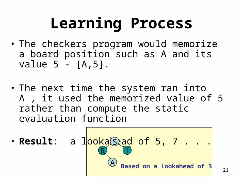
Learning Process• The checkers program would memorize a board

position such as A and its value 5 - [A,5].

• The next time the system ran into A , it used the memorized value of 5 rather than compute the static evaluation function

• Result: a lookahead of 5, 7 . . .

SR T

A Based on a lookahead of 3

22

Introduction to Learning by Induction

Learning by Example• Learning by induction is a general learning strategy

where a concept is learned by drawing inductive inferences from a set of facts

• AI systems that learn by example can be viewed as searching a concept space by means of a decision tree

• The best known approach to constructing a decision tree is called ID3

Iterative Dichotomizer 3 - developed byJ. Ross Quinlan in 1975

23

ID3 Process

• ID3 begins with a set of examples (known facts)

• It ends with a set of rules in the form of a decision tree which may then be applied to unknown cases

• It works by recursively splitting the example set into smaller sets in the most efficient manner possible.

24

Possible QuizPossible QuizWhat is inductive learning?

How does rote learning work?

What is ID3?

Summary•Introduction to Learning

•Learning Methods

•Introduction to Learning by Induction

25

Review – Learning by ExampleReview – Learning by Example

• Learning by induction is a general learning strategy where a concept is learned by drawing inductive inferences from a set of facts

• AIl systems that learn by example can be viewed as searching a concept space by means of a decision tree

• The best known approach to constructing a decision tree is called ID3

26

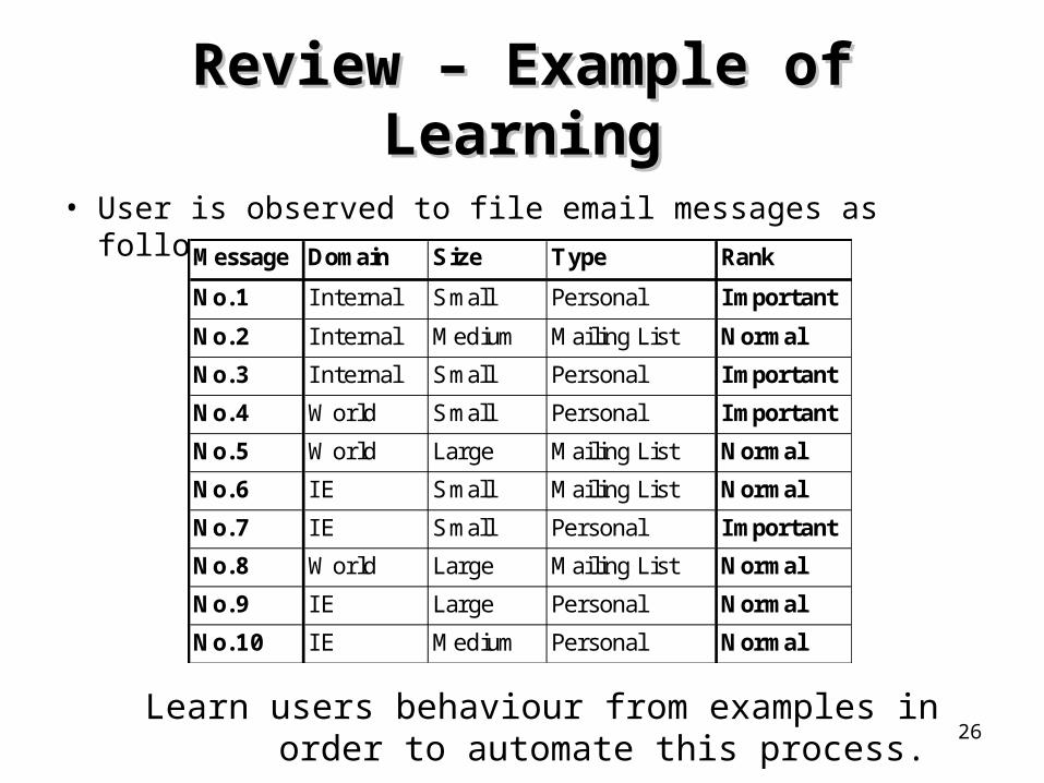
Review – Example of LearningReview – Example of Learning

• User is observed to file email messages as follows:-Message Domain Size Type Rank

No.1 I nternal Small Personal Important

No.2 I nternal Medium Mailing List Normal

No.3 I nternal Small Personal Important

No.4 World Small Personal Important

No.5 World Large Mailing List Normal

No.6 I E Small Mailing List Normal

No.7 I E Small Personal Important

No.8 World Large Mailing List Normal

No.9 I E Large Personal Normal

No.10 I E Medium Personal Normal

Learn users behaviour from examples in order to automate this process.

27

OUTLINE

• Background

• Decision Trees

• ID3

28

Background

• We are interested in datasets consisting of a number of records

• Each record has:– A set of attribute-value pairs

E.g. “Color: green, Temperature: 120oC”– A classification

E.g. “Risk: Low”

• We assume that the classification is dependent on the attributes– We are assuming that the dataset “makes sense”

29

Inductive Learning

• Interesting problem: Can we find the mapping between the attributes and the classifications only using the dataset?

• This is the purpose of an inductive learning algorithm

• In practice, we can only find an approximation to the true mapping– Only a hypothesis, but still useful:

• Classification of new records (prediction)• Identifying patterns in the dataset (data mining)

30

Classification Problem

• We model each record as a pair (x, y), where x is the set of attributes and y is the classification

• We are trying to find a function f which models the data:– We want to find f such that f(x) = y for as many

records in the dataset as possible

• To make things easier, we will use a fixed set of attributes and discrete classes

31

Choosing a Classifier

• Some issue to consider:– Construction time– Runtime performance– Transparency– Updateability– Scalability

• All these rest on how f is represented by the model

32

Common Classifiers

• Analytical (mathematical) models

• Nearest-neighbor classifiers

• Neural networks

• Genetic programming

• Genetic algorithms (classifier systems)

• Decision trees

33

Decision Trees

• What is a Decision Tree?– it takes as input the description of a situation as a set

of attributes (features) and outputs a yes/no decision (so it represents a Boolean function)

– each leaf is labeled "positive” or "negative", each node is labeled with an attribute (or feature), and each edge is labeled with a value for the feature of its parent node

• Attribute-value language for examples– in many inductive tasks, especially learning decision

trees, we need a representation language for examples

• each example is a finite feature vector• a concept is a decision tree where nodes are features

34

History

• Independently developed in the 60’s and 70’s by researchers in ...– Statistics: L. Breiman & J. Friedman - CART

(Classification and Regression Trees)– Pattern Recognition: Uof Michigan - AID,

G.V. Kass - CHAID (Chi-squared Automated Interaction Detection)

– AI and Info. Theory: R. Quinlan - ID3, C4.5 (Iterative Dichotomizer)

35

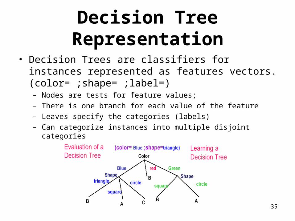
Decision Tree Representation

• Decision Trees are classifiers for instances represented as features vectors. (color= ;shape= ;label=)– Nodes are tests for feature values;

– There is one branch for each value of the feature

– Leaves specify the categories (labels)

– Can categorize instances into multiple disjoint categories

36

Example

• Problem: How do you decide to leave a restaurant?

• Variables:

Alternative Whether there is a suitable alternative restaurant nearby. Bar Is there a comfortable bar area?Fri/Sat True on Friday or Saturday nights.Hungary How hungry is the subject?Patrons How many people in the restaurant?Price Price range.Raining Is it raining outside?Reservation Does the subject have a reservation?Type Type of Restaurant.Stay? Stay or Go

37

38

39

How?

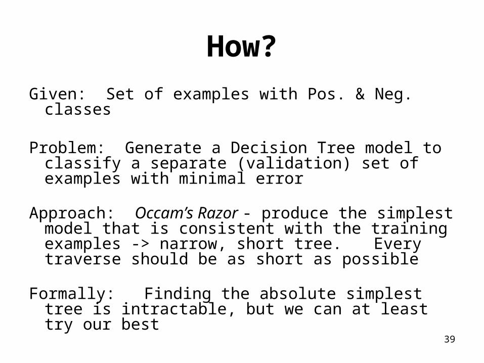
Given: Set of examples with Pos. & Neg. classes

Problem: Generate a Decision Tree model to classify a separate (validation) set of examples with minimal error

Approach: Occam’s Razor - produce the simplest model that is consistent with the training examples -> narrow, short tree. Every traverse should be as short as possible

Formally: Finding the absolute simplest tree is intractable, but we can at least try our best

40

Exhaustive Search

• We could try to build every possible tree and the select the best one

• How many trees are there for a specific problem?– Given a dataset with 5 different binary

attributes– How many trees are there in this case?

41

Answer

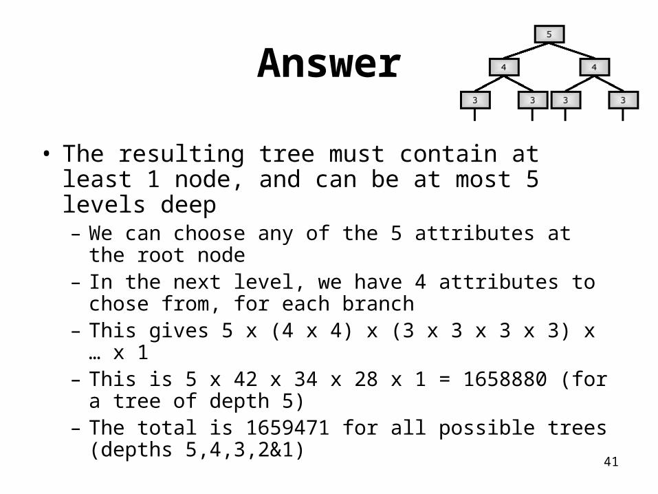
• The resulting tree must contain at least 1 node, and can be at most 5 levels deep– We can choose any of the 5 attributes at the root

node– In the next level, we have 4 attributes to chose from,

for each branch– This gives 5 x (4 x 4) x (3 x 3 x 3 x 3) x … x 1– This is 5 x 42 x 34 x 28 x 1 = 1658880 (for a tree of

depth 5)– The total is 1659471 for all possible trees (depths

5,4,3,2&1)

42

Producing the Best DT

Heuristic (strategy) 1: Grow the tree from the top down. Place the most important variable test at the root of each successive subtree

The most important variable: – the variable (predictor) that gains the most ground in

classifying the set of training examples – the variable that has the most significant relationship

to the response variable– to which the response is most dependent or least

independent

43

ID3 Process

• ID3 begins with a set of examples (known facts)

• It ends with a set of rules in the form of a decision tree which may then be applied to unknown cases

• It works by recursively splitting the example set into smaller sets in the most efficient manner possible.

44

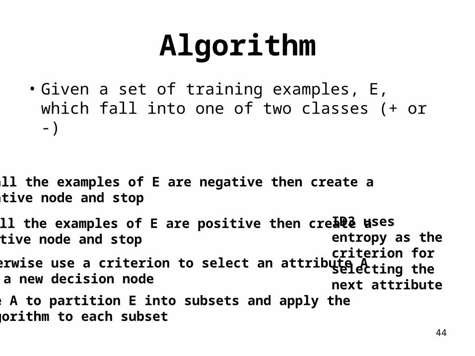
Algorithm

• Given a set of training examples, E, which fall into one of two classes (+ or -)

If all the examples of E are negative then create anegative node and stop

If all the examples of E are positive then create apositive node and stop

Otherwise use a criterion to select an attribute Afor a new decision node

Use A to partition E into subsets and apply thealgorithm to each subset

ID3 uses entropy as the criterion for selecting thenext attribute

45

Aside: Entropy

• Entropy is the basis of Information Theory

• Entropy is a measure of randomness, hence the smaller the entropy the greater the information content

• Given a message with n symbols in which the ith symbol has probability pi of appearing, the entropy of the message is:

H = - (pilog2pi)i=1

n

46

Entropy in ID3

• For a selected attribute value A = vi, determine the number of examples with vi that are negative (Nn) and the number of examples with vi that are positive (Np).

H =-i=1

n

[Nplog2(Np + Nn

Np ) + Nnlog2(Np + Nn

Nn )]

47

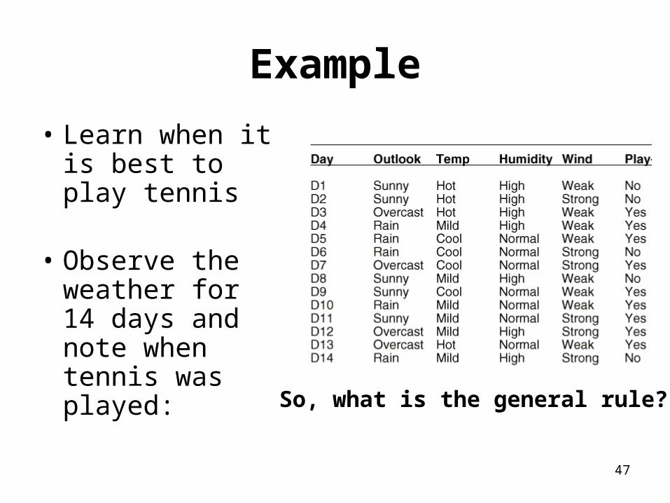
Example

• Learn when it is best to play tennis

• Observe the weather for 14 days and note when tennis was played: So, what is the general rule?

48

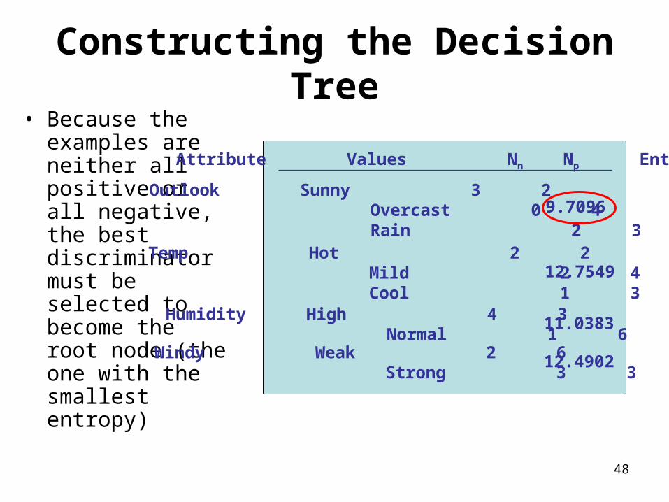
Constructing the Decision Tree• Because the

examples are neither all positive or all negative, the best discriminator must be selected to become the root node (the one with the smallest entropy)

Outlook Sunny 3 2 Overcast 0 4 Rain 2 3

Attribute Values Nn Np Entropy

Temp Hot 2 2 Mild 2 4 Cool 1 3 Humidity High 4 3 Normal 1 6Windy Weak 2 6 Strong 3 3

9.7096

12.7549

11.0383

12.4902

49

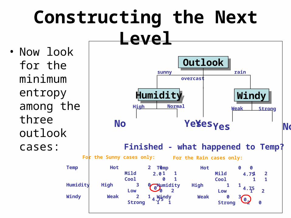
Constructing the Next Level• Now look for

the minimum entropy among the three outlook cases:

OutlookOutlooksunny

overcastrain

For the Sunny cases only:

Temp Hot 2 0 Mild 1 1 Cool 0 1Humidity High 3 0 Low 0 2Windy Weak 2 1 Strong 1 1

2.0

0

4.75

HumidityHumidityHigh Normal

No Yes Yes

For the Rain cases only:

Temp Hot 0 0 Mild 1 2 Cool 1 1Humidity High 1 1 Low 1 2Windy Weak 0 3 Strong 2 0

4.75

4.75

0

WindyWindyWeak Strong

Yes No

Finished - what happened to Temp?

50

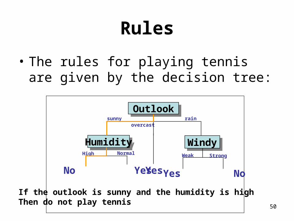
Rules

• The rules for playing tennis are given by the decision tree:

OutlookOutlooksunny

overcastrain

HumidityHumidityHigh Normal

No Yes Yes

WindyWindyWeak Strong

Yes No

If the outlook is sunny and the humidity is highThen do not play tennis

51

Possible QuizPossible Quiz

What is the purpose of an inductive learning algorithm?

What is Entropy?

What variable is placed at the root node of a Decision Tree?

Summary•Background

•Decision Trees

•ID3

52

Review – Decision TreesReview – Decision Trees

• What is a Decision Tree?– it takes as input the description of a situation as a set

of attributes (features) and outputs a yes/no decision (so it represents a Boolean function)

– each leaf is labeled "positive” or "negative", each node is labeled with an attribute (or feature), and each edge is labeled with a value for the feature of its parent node

• ID3 is one example of an algorithm that will create a Decision Tree

53

Review – AdvantagesReview – Advantages

• Proven modeling method for 20 years

• Provides explanation and prediction

• Useful for non-linear mappings

• Generalizes well given sufficient examples

• Rapid training and recognition speed

• Has inspired many inductive learning algorithms using statistical regression

54

Review - Disadvantages

• Only one response variable at a time• Different significance tests required for

nominal and continuous responses• Discriminate functions are often

suboptimal due to orthogonal decision hyperplanes

• No proof of ability to learn arbitrary functions

• Can have difficulties with noisey data

55

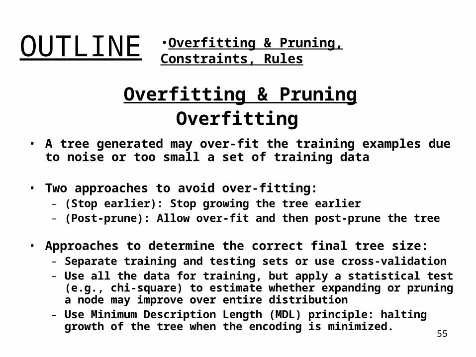
Overfitting & Pruning Overfitting

• A tree generated may over-fit the training examples due to noise or too small a set of training data

• Two approaches to avoid over-fitting:– (Stop earlier): Stop growing the tree earlier– (Post-prune): Allow over-fit and then post-prune the tree

• Approaches to determine the correct final tree size:– Separate training and testing sets or use cross-validation– Use all the data for training, but apply a statistical test

(e.g., chi-square) to estimate whether expanding or pruning a node may improve over entire distribution

– Use Minimum Description Length (MDL) principle: halting growth of the tree when the encoding is minimized.

OUTLINE •Overfitting & Pruning, Constraints, Rules

56

Overfitting Effects

• The effect of overfitting is that it produces a tree that works very well on the training set but produces a lot of errors on the test set

Accuracy on training and test data

57

Avoiding Overfitting

• Two basic approaches– Prepruning: Stop growing the tree at some point

during construction when it is determined that there is not enough data to make reliable choices.

– Postpruning: Grow the full tree and then remove nodes that seem not to have sufficient evidence.

• Methods for evaluating subtrees to prune: – Cross-validation: Reserve hold-out set to evaluate

utility– Statistical testing: Test if the observed regularity can

be dismissed as likely to be occur by chance – Maximum Description Length: Is the additional

complexity of the hypothesis smaller than remembering the exceptions

58

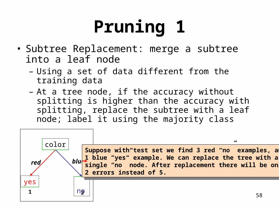
Pruning 1• Subtree Replacement: merge a subtree into

a leaf node– Using a set of data different from the training

data– At a tree node, if the accuracy without splitting is

higher than the accuracy with splitting, replace the subtree with a leaf node; label it using the majority class

color

yes no

red blue

1 2

Suppose with test set we find 3 red “no” examples, and1 blue “yes” example. We can replace the tree with a single “no” node. After replacement there will be only2 errors instead of 5.

Suppose with test set we find 3 red “no” examples, and1 blue “yes” example. We can replace the tree with a single “no” node. After replacement there will be only2 errors instead of 5.

59

Pruning 2

• A post-pruning, cross validation approach– Partition training data into “grow” set and “validation”

set.– Build a complete tree for the “grow” data– Until accuracy on validation set decreases, do:

• For each non-leaf node in the tree • Temporarily prune the tree below; replace it by majority vote.• Test the accuracy of the hypothesis on the validation set• Permanently prune the node with the greatest increase in

accuracy on the validation test

60

Constraints Motivation

• Necessity of Constraints– Decision tree can be

• Complex with hundreds or thousands of nodes• Difficult to comprehend

– Users are only interested in obtaining an overview of the patterns in their data

• A simple, comprehensible, but only approximate decision tree is much more useful

• Necessity of Pushing constraints into the tree-building phase – In tree-building phase, may waste I/O on building tree

which will be pruned by applying constraints

61

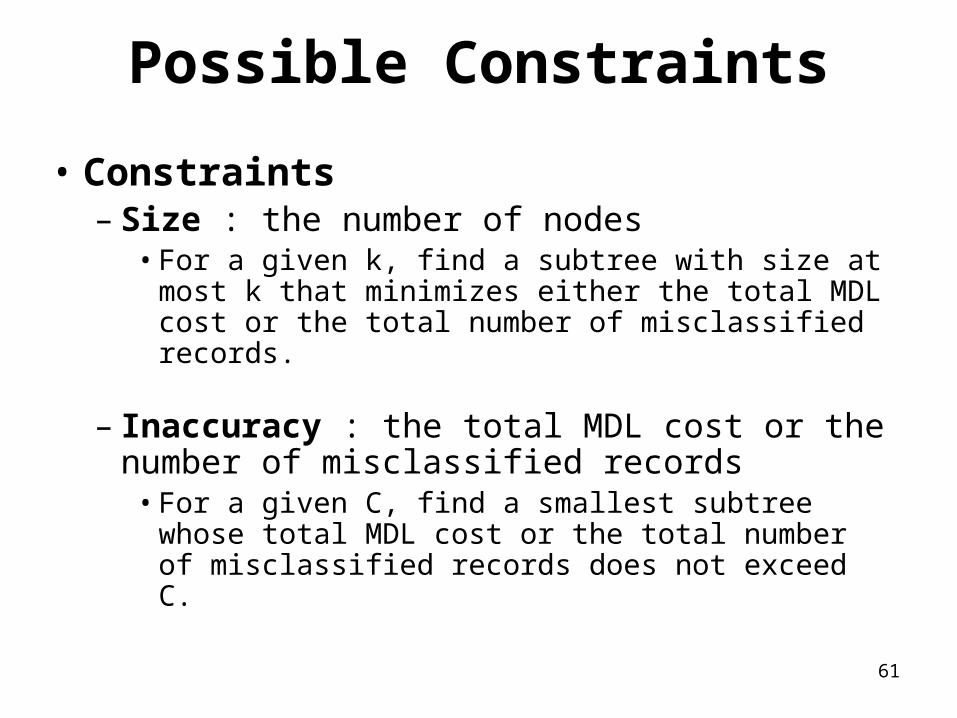
Possible Constraints

• Constraints– Size : the number of nodes

• For a given k, find a subtree with size at most k that minimizes either the total MDL cost or the total number of misclassified records.

– Inaccuracy : the total MDL cost or the number of misclassified records

• For a given C, find a smallest subtree whose total MDL cost or the total number of misclassified records does not exceed C.

62

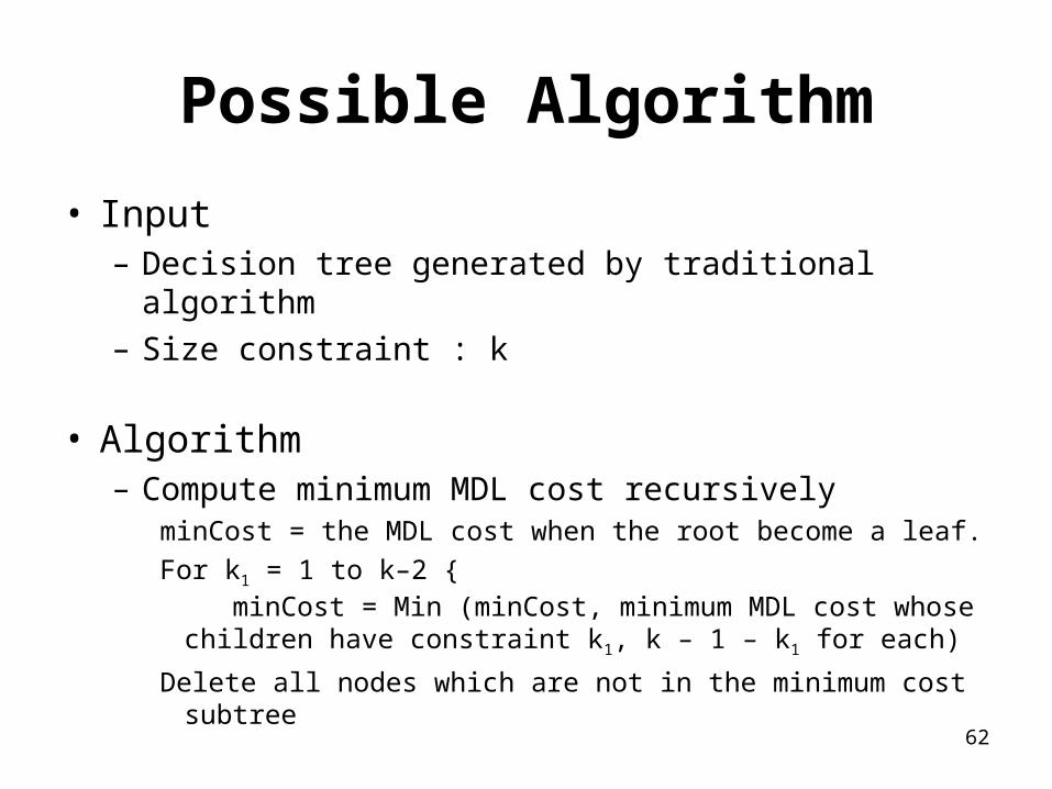
Possible Algorithm

• Input– Decision tree generated by traditional algorithm– Size constraint : k

• Algorithm– Compute minimum MDL cost recursively

minCost = the MDL cost when the root become a leaf.

For k1 = 1 to k–2 { minCost = Min (minCost, minimum MDL cost whose children have constraint k1, k – 1 – k1 for each)

Delete all nodes which are not in the minimum cost subtree

63

RULES DT to Rules

• A Decision Tree can be converted into a rule set– Straightforward conversion: rule set overly complex– More effective conversions are not trivial

• Strategy for generating a rule set directly: for each class in turn find rule set that covers all instances in it (excluding instances not in the class)

• This approach is called a covering approach because at each stage a rule is identified that covers some of the instances

64

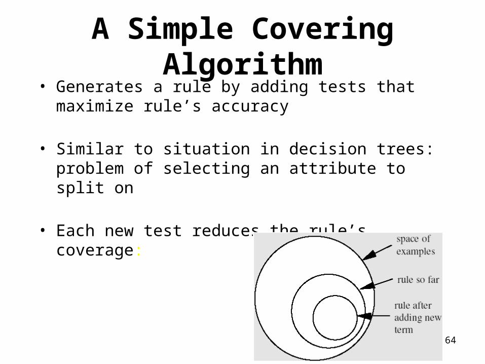
A Simple Covering Algorithm• Generates a rule by adding tests that maximize rule’s

accuracy

• Similar to situation in decision trees: problem of selecting an attribute to split on

• Each new test reduces the rule’s coverage:

65

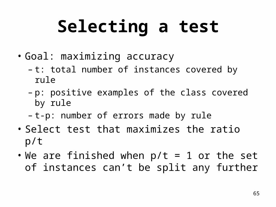
Selecting a test

• Goal: maximizing accuracy– t: total number of instances covered by rule– p: positive examples of the class covered by

rule– t-p: number of errors made by rule

• Select test that maximizes the ratio p/t

• We are finished when p/t = 1 or the set of instances can’t be split any further

66

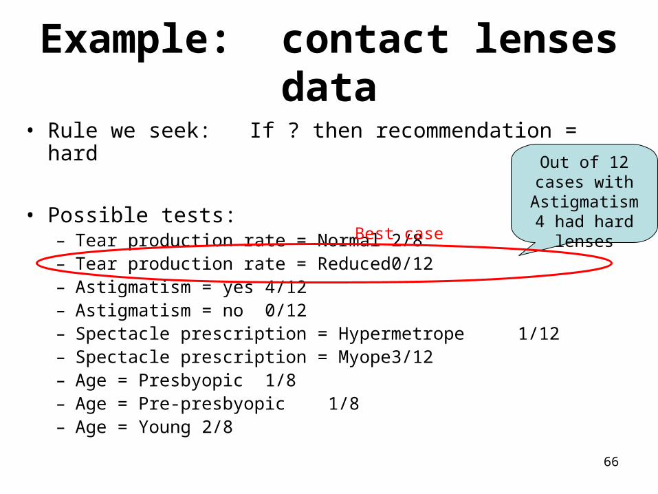
Example: contact lenses data

• Rule we seek: If ? then recommendation = hard

• Possible tests:– Tear production rate = Normal 2/8– Tear production rate = Reduced 0/12– Astigmatism = yes 4/12– Astigmatism = no 0/12– Spectacle prescription = Hypermetrope 1/12– Spectacle prescription = Myope 3/12– Age = Presbyopic 1/8– Age = Pre-presbyopic 1/8– Age = Young 2/8

Out of 12 cases with

Astigmatism 4 had hard lenses

Best case

67

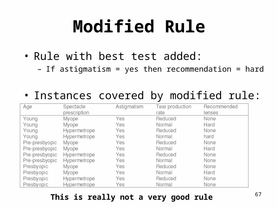
Modified Rule

• Rule with best test added:– If astigmatism = yes then recommendation = hard

• Instances covered by modified rule:

This is really not a very good rule

68

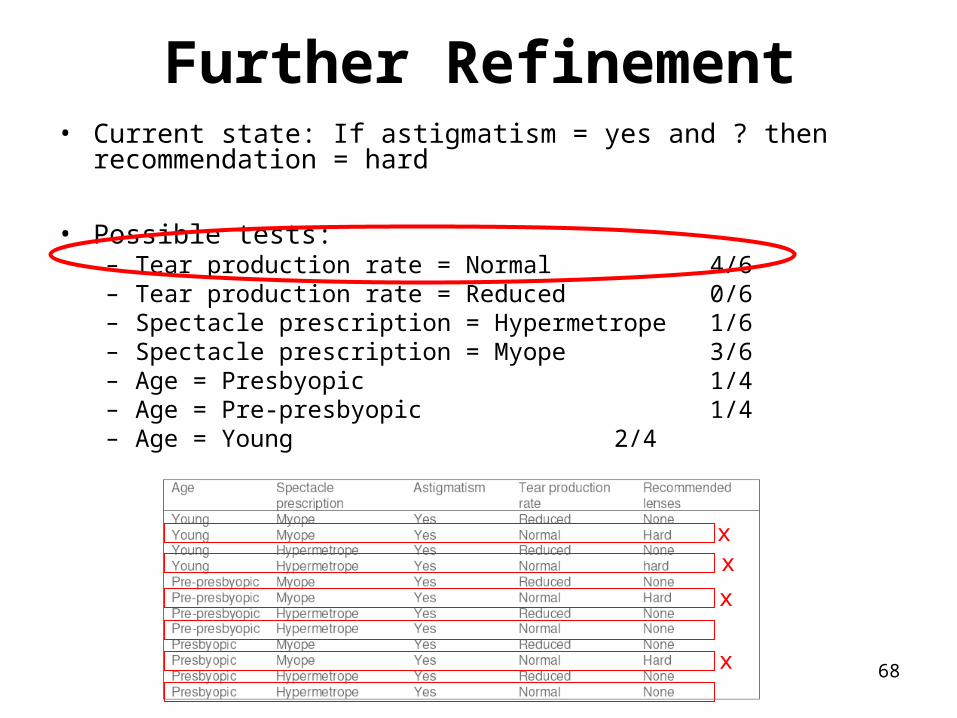
Further Refinement• Current state: If astigmatism = yes and ? then recommendation =

hard

• Possible tests:– Tear production rate = Normal 4/6– Tear production rate = Reduced 0/6– Spectacle prescription = Hypermetrope 1/6– Spectacle prescription = Myope 3/6– Age = Presbyopic 1/4– Age = Pre-presbyopic 1/4– Age = Young 2/4

xx

x

x

69

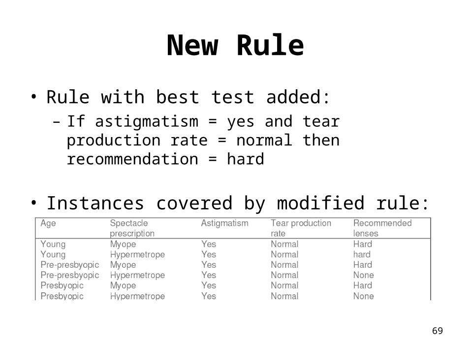
New Rule

• Rule with best test added:– If astigmatism = yes and tear production rate =

normal then recommendation = hard

• Instances covered by modified rule:

70

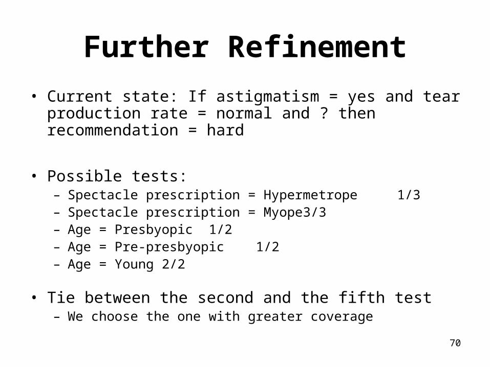
Further Refinement

• Current state: If astigmatism = yes and tear production rate = normal and ? then recommendation = hard

• Possible tests:– Spectacle prescription = Hypermetrope 1/3– Spectacle prescription = Myope 3/3– Age = Presbyopic 1/2– Age = Pre-presbyopic 1/2– Age = Young 2/2

• Tie between the second and the fifth test– We choose the one with greater coverage

71

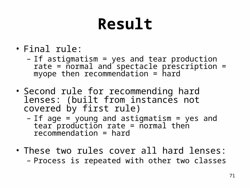
Result

• Final rule:– If astigmatism = yes and tear production rate =

normal and spectacle prescription = myope then recommendation = hard

• Second rule for recommending hard lenses: (built from instances not covered by first rule)– If age = young and astigmatism = yes and tear

production rate = normal then recommendation = hard

• These two rules cover all hard lenses:– Process is repeated with other two classes

72

Possible QuizPossible QuizWhat is overfitting?

What is pruning?

Name one possible constraint.

SUMMARY•Overfitting & Pruning

•Constraints

•Rules

73

Supervised Learning

• In supervised learning, the network is presented with inputs together with the target (teacher signal) outputs.

• Then, the neural network tries to produce an output as close as possible to the target signal by adjusting the values of internal weights.

• The most common supervised learning method is the “error correction method”

74

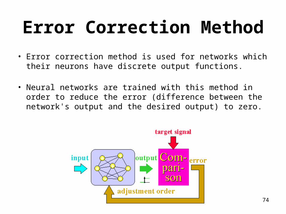
Error Correction Method

• Error correction method is used for networks which their neurons have discrete output functions.

• Neural networks are trained with this method in order to reduce the error (difference between the network's output and the desired output) to zero.

75

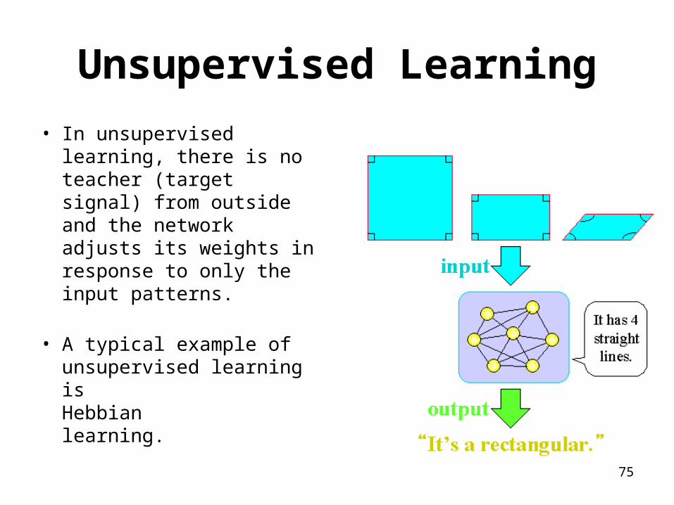
Unsupervised Learning

• In unsupervised learning, there is no teacher (target signal) from outside and the network adjusts its weights in response to only the input patterns.

• A typical example of unsupervised learning is Hebbian learning.

76

Common NN Features

• “weight” = strength of connection

• threshold = value of weighted input below which no response is produced

• signals may be:– real-valued, or– binary-valued:

• “unipolar” {0, 1}• “bipolar” {-1, 1}

77

McCulloch/Pitts Neuron

• One of the first neuron models to be implemented

• Its output is 1 (fired) or 0

• Each input is weighted with weights in the range -1 to + 1

• It has a threshold value, T

Tw1

w2

w3

x1

x2

x3

The neuron fires if the followinginequality is true:

x1w1 + x2w2 + x3w3 > T

78

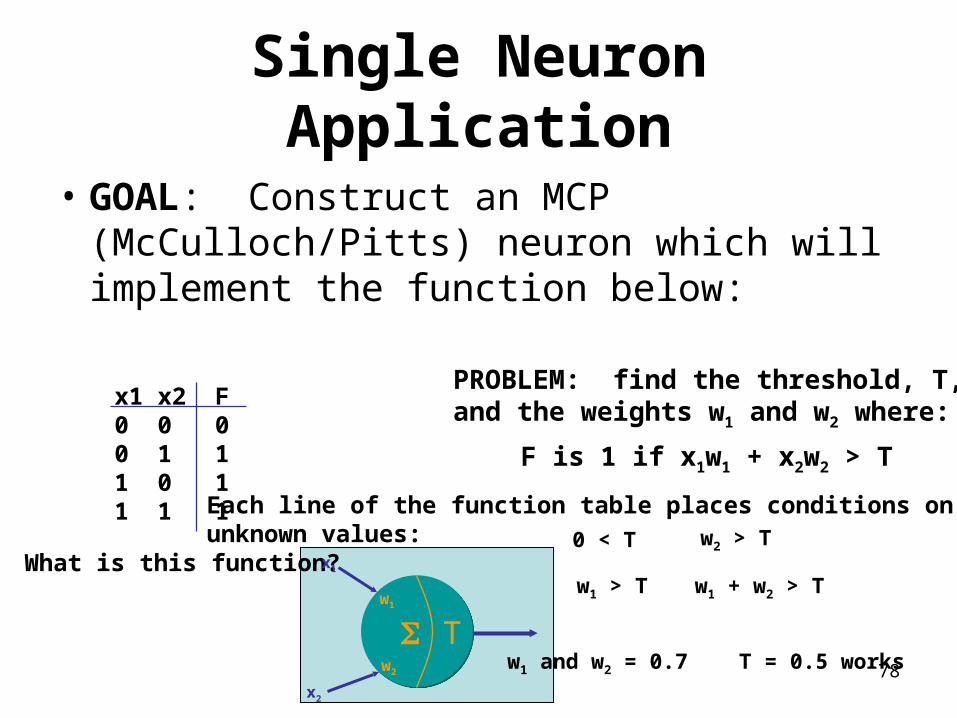
Single Neuron Application

• GOAL: Construct an MCP (McCulloch/Pitts) neuron which will implement the function below:

x1 x2 F0 0 00 1 11 0 11 1 1

What is this function?

Tw1

w2

x1

x2

PROBLEM: find the threshold, T, and the weights w1 and w2 where:

F is 1 if x1w1 + x2w2 > T

Each line of the function table places conditions on theunknown values: 0 < T

w1 > T

w2 > T

w1 + w2 > T

w1 and w2 = 0.7 T = 0.5 works

79

NN Development

• There is no single methodology for NN development– A suggested

approach is:

Data Selection, Preparation,

Preprocessing

Determine Best-SuitedAlgorithm

Define Problem

Train Network

Trained Successfully?

Test Network

Tested Successfully?

Run/Use Network

80

Learning in Neural Nets (again)

• The operation of a neural network is determined by the values of the interconnection weights– There is no algorithm that determines how the

weights should be assigned in order to solve a specific problems

– Hence, the weights are determined by a learning process

81

Hebbian Learning

• The oldest and most famous of all learning rules is Hebb’s postulate of learning:

“When an axon of cell A is near enough to excite a cell Band repeatedly or persistently takes part in firing it, somegrowth process or metabolic changes take place in one orboth cells such that A’s efficiency as one of the cells firingB is increased”

Application to artificial neurons:

If two interconnected neurons are both “on” at the sametime, then the weight between them should be increased

82

Hebb’s Algorithm

• Step 0: initialize all weights to 0

• Step 1: Given a training input, s, with its target output, t, set the activations of the input units: xi = si

• Step 2: Set the activation of the output unit to the target value: y = t

• Step 3: Adjust the weights: wi(new) = wi(old) + xiy

• Step 4: Adjust the bias (just like the weights): b(new) = b(old) + y

83

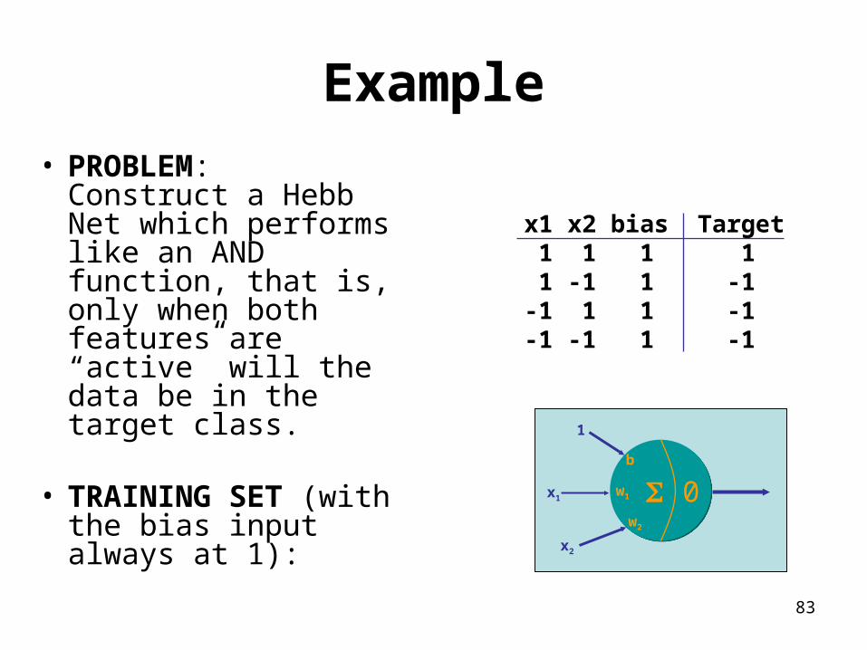
Example

• PROBLEM: Construct a Hebb Net which performs like an AND function, that is, only when both features are “active” will the data be in the target class.

• TRAINING SET (with the bias input always at 1):

x1 x2 bias Target 1 1 1 1 1 -1 1 -1-1 1 1 -1-1 -1 1 -1

0w1

w2

x1

x2

1

b

84

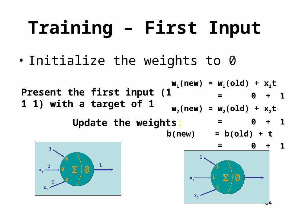
Training – First Input

• Initialize the weights to 0

00

0

x1

x2

1

0

Present the first input (1 1 1) with a target of 1

Update the weights:

w1(new) = w1(old) + x1t

w2(new) = w2(old) + x2t

= 0 + 1 = 1

= 0 + 1 = 1

b(new) = b(old) + t

= 0 + 1 = 1

01

1

x1

x2

1

11

1

1

85

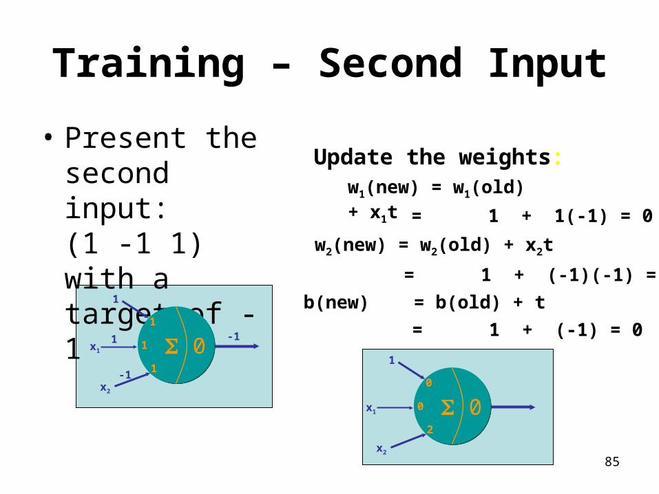
Training – Second Input

• Present the second input: (1 -1 1) with a target of -1

01

1

x1

x2

1

1

00

2

x1

x2

1

0

Update the weights:w1(new) = w1(old) + x1t

w2(new) = w2(old) + x2t

= 1 + 1(-1) = 0

= 1 + (-1)(-1) = 2

b(new) = b(old) + t

= 1 + (-1) = 0 -1

-1

1

86

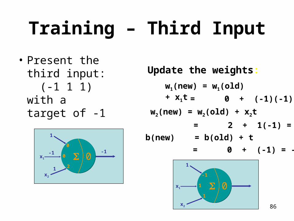
Training – Third Input

• Present the third input: (-1 1 1) with a target of -1

00

2

x1

x2

1

0

01

1

x1

x2

1

-1

Update the weights:

w1(new) = w1(old) + x1t

w2(new) = w2(old) + x2t

= 0 + (-1)(-1) = 1

= 2 + 1(-1) = 1

b(new) = b(old) + t

= 0 + (-1) = -1 -1

1

-1

87

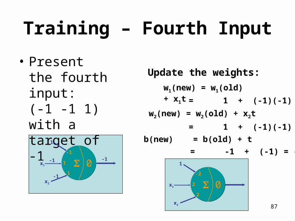
Training – Fourth Input

• Present the fourth input: (-1 -1 1) with a target of -1

01

1

x1

x2

1

-1

02

2

x1

x2

1

-2

Update the weights:

w1(new) = w1(old) + x1t

w2(new) = w2(old) + x2t

= 1 + (-1)(-1) = 2

= 1 + (-1)(-1) = 1

b(new) = b(old) + t

= -1 + (-1) = -2 -1

-1

-1

88

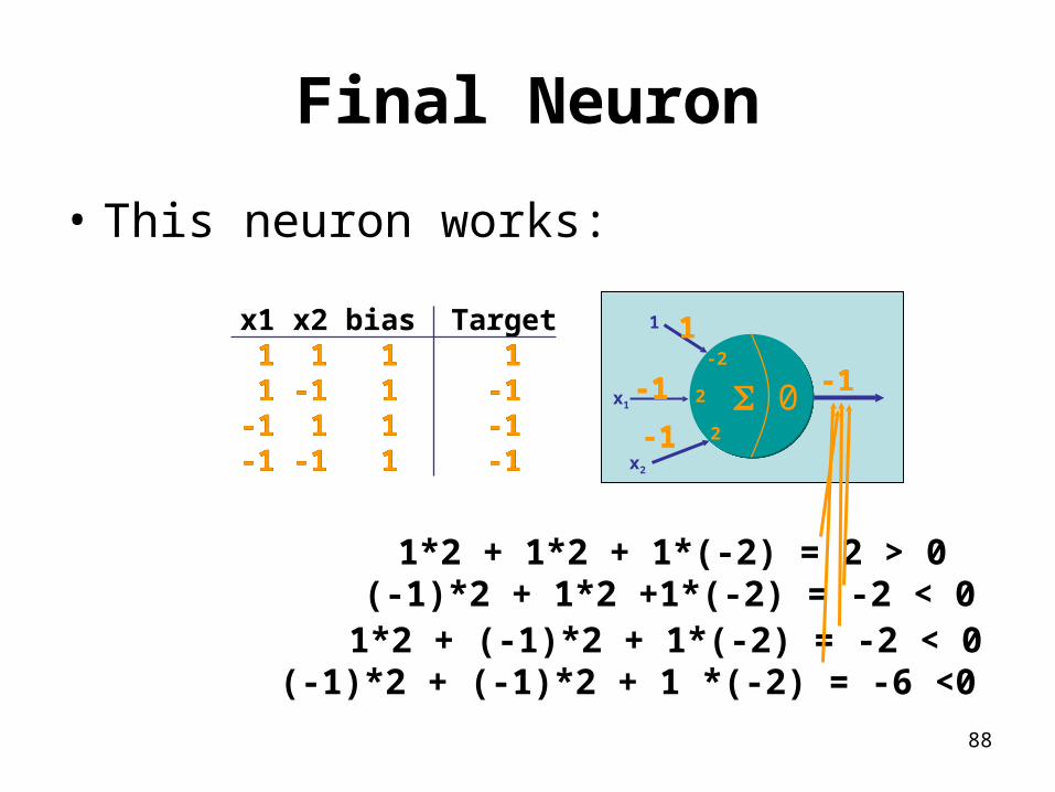
Final Neuron

• This neuron works:

02

2

x1

x2

1

-2

x1 x2 bias Target 1 1 1 1 1 -1 1 -1-1 1 1 -1-1 -1 1 -1

1 1 1 11

1

1

1*2 + 1*2 + 1*(-2) = 2 > 0

11 -1 1 -1

1

1

-1

-1

(-1)*2 + 1*2 +1*(-2) = -2 < 0

-1-1 1 1 -1

-1

1

1

1*2 + (-1)*2 + 1*(-2) = -2 < 0(-1)*2 + (-1)*2 + 1 *(-2) = -6 <0

-1

1

-1

-1

-1 -1 1 -1

89

Possible QuizPossible QuizWhat is the difference between supervised andunsupervised learning?

What is the principle behind Hebbian learning?

Describe a MP Neuron.

SUMMARYFeatures of Neural Nets

Learning in Neural Nets

McCulloch/Pitts Neuron

Hebbian Learning