1 Regular singular points of differential equa- tions ...

1 Regular singular points of differential equa-tions, nondegenerate case

Consider the system

w′ =1zBw + A1(z)w (1)

where B is a constant matrix and A1 is analytic at zero. Assume no two eigen-values of B differ by an positive integer. Let J be the Jordan normal form of B.As usual, by a linear change of variables, we can bring (1) to the normal form

y′ =1zJy + A(z)y (2)

where A(z) is analytic.

Theorem 1. Under the assumptions above, (1) has a fundamental matrix so-lution in the form M(z) = Y (z)zB, where Y (z) is a matrix analytic at zero.

Proof. Clearly, it is enough to prove the theorem for (2). We look for a solutionof (2) in the form M = Y zJ , where

Y (z) = J + zY1 + z2Y2 + · · · (3)

we get

Y ′zJ +1zY JzJ =

1zJY zJ + AY zJ (4)

Multiplying by z−J we obtain

Y ′ +1zY J =

1zJY + AY (5)

orY ′ =

1z

(JY − Y J

)+ AY (6)

Expanding out, we get

Y1 + 2zY2 + 3z2Y3 + · · · =[(JY1 − Y1J) + z(JY2 − Y2J) + · · ·

]+ A0J + zA1J + · · ·+ zA0Y1 + z2(A0Y2 + A1Y1) + · · · (7)

The associated system of equations, after collecting the powers of z is

kYk = (JYk − YkJ) + AkJ +k−2∑l=0

AlYk−1−l; k ∈ N (8)

or

VkYk = Ak−1J +k−2∑l=0

AlYk−1−l; k ∈ N (9)

1

whereVkM := kM − (JM −MJ) (10)

is a linear operator on matrices M ∈ Rn2. As a linear operator on a finite

dimensional space, VkX = Y has a unique solution for every Y iff detVk 6= 0or, which is the same, VkX = 0 implies X = 0.

We show that this is the case.Let v be one of the eigenvectors of J . If VkX = 0 we obtain,

k(Xv)− J(Xv) + Xλv = 0 (11)

ork(Xv)− J(Xv) + Xλv = 0 (12)

J(Xv) = (λ + k)(Xv) (13)

Since λ + k is not an eigenvalue of J , this forces Xv = 0. We take the nextgeneralized eigenvector, w, in the same Jordan block as v, if any.

We remind that we have the following relations between these generalizedeigenvectors:

Jvi = λvi + vi−1 (14)

where v0 = v is an eigenvector and 1 ≤ i ≤ m− 1 where m is the dimension ofthe Jordan block.

We havek(Xw)− J(Xw) + X(λw + v) = 0 (15)

and since Xv = 0 we get

J(Xw) = (λ + k)(Xw) (16)

and thus Xw = 0. Inductively, we see that Xv = 0 for any generalized eigen-vector of J , and thus X = 0.

Now, we claim that V −1k ≤ Ck−1 for some C. We let C be the commutator

operator, CX = JX −XJ Now ‖JX −XJ‖ ≤ 2‖J‖‖X‖ and thus

V −1k = k−1

(I − k−1C

)−1= k−1(1 + o(1)); (k →∞) (17)

Therefore, the function kVk is bounded for k ∈ R+.We rewrite the system (8) in the form

Yk = V −1k Ak−1J + V −1

k

k−2∑l=0

AlYk−1−l; k ∈ N (18)

or, in abstract form, with Y = {Yj}j∈N, (LY)k := V −1k

∑k−2l=0 AlYk−1−l, where

we regard Y as a function defined on N with matrix values, with the norm

‖Y‖ = supn∈N

‖µ−nY(n)‖; µ > 1 (19)

we haveY = Y0 + LY (20)

2

Exercise 1. Show that (20) is contractive for µ sufficiently large, in an appro-priate ball that you will find.

2 Changing the eigenvalue structure of J by trans-formations

Assume we want to make a transformation so that all eigenvalues of the newsystem are unchanged, except for one of them which we would like to decreaseby one. We write J in the form (

J1 00 J2

)(21)

where J1 is the Jordan block we care about, dim(J1) = m ≥ 1, while J2 isa Jordan matrix, consisting of the remaining blocks. Suppose for now thatthe assumptions of Theorem1 are satisfied. The fundamental solution of y′ =z−1Jy+A(z)y is of the form M = Y (z)zJ . Suppose we make the transformation

M1 = M

(z−I 00 I

)= MS

S =(

z−1I 00 I

)(22)

with the diagonal block sizes, counting from above, m and n−m. Then,

MS =(

Y11 Y12

Y13 Y14

)(zJ1 00 zJ2

)(z−I 00 I

)=(

Y11 Y12

Y13 Y14

)(zJ1−I 0

0 zJ2

)(23)

where Yij are matrices, dim(Y11) = dim(Y21) = m, dim(Y12) = dim(Y22) =n−m. The modified matrix, MS, has a structure that would correspond to theJordan matrix (

J1 − I 00 J2

)(24)

and thus to a new B with eigenvalues as described at the beginning of thesection. The change of variable Sy = w, or y = S−1w = Uw where, clearly,

U = S−1 =(

zI 00 I

)(25)

is natural, the only question is whether the new equation is of the same type.So, let’s check. Let y = Uw. Then, we have

U ′w + Uw′ =1zJUw + AUw (26)(

I 00 0

)w +

(zI 00 I

)w′ =

1zJUw + AUw (27)

3

w′ =(

z−1I 00 I

)(J1 − I

0 J2

)1z

(zI 00 I

)w

+(

z−1I 00 I

)(A11 A12

A21 A21

)(zI 00 I

)(28)

or

w′ =1z

(J1 − I A12(0)

0 J2

)+ A1w =

1zB1w + A1w (29)

where Aik are matrices of the same dimensions as Yik. The eigenvalues of B1

are now λ1 − 1, λ2, ....

Exercise 1. Use this procedure repeatedly to reduce any resonant system to anonresonant one. That is done by arranging that the eigenvalues that differ bypositive integers become equal.

Exercise 2. Use Exercise 1 to prove the following result.

Theorem 2. Any system of the form

y′ =1zB(z)y (30)

where B is an analytic matrix at zero, has a fundamental solution of the form

M(z) = Y (z)zB′(31)

where B′ is a constant matrix, and Y is analytic at zero. In the nonresonantcase, B′ = B(0).

Note that this applies even if B(0) = 0.

Exercise 3. Find B′ in the case where only two eigenvalues differ by a positiveinteger, where the integer is 1.

3 Scalar n−th order linear equations

These are equations of the form

y(n) + a1(z)y(n−1) + · · ·+ an(z)y = 0 (32)

Such an equation can always be transformed into a system of the form w′ =A(x)w, and viceversa. There are many ways to do that. The simplest is to takev0 = y, ..., vk = y(k), ... and note that (32) is equivalent to

v0

v1

· · ·vn−1

′

=

0 1 0 · · · 00 0 1 · · · 0

· · ·−an(z) −an−1(z) −an−2(z) · · · −a1(z)

v0

v1

· · ·vn−1

(33)

4

In the other direction, to simplify notation assume n = 2. The system is then

y′ = a(x)y + b(x)ww′ = c(x)y + d(x)w (34)

We differentiate one more time say, the second equation, and get

w′′ = dw′ + (bc + d′)w + (ac + c′)y (35)

If c ≡ 0, then (35) is already of the desired form. Otherwise, we write

y =1cw′ − d

cw (36)

and substitute in (35). The result is

w′′ =(

a + d +c′

c

)w′ +

(c

(d

c

)′+ [cb− ad]

)w (37)

Note that a and c, by assumptions, have at most first order poles, while c′/c hasat most simple poles for any analytic function. Therefore, the emergent secondorder equation has the general form

w′′ + a1(x)w′ + a2(x)w = 0

where ai has a pole of order at most i.

Exercise 1. Generalize this transformation procedure to nth order systems.Show that the resulting nth order equation is of the general form

y(n) + a1y(n−1) + · · ·+ any = 0 (38)

where the coefficients ai are analytic in Dρ \ {0} and have a pole of order atmost i at zero.

Definition 1. An equation of the form (38) has a singularity of the first kindat zero if the conditions of Exercise 1 are met.

Definition 2. An equation of the form (38) has a regular singularity at zero ifthere exists a fundamental set of solutions in the form of finite combinations offunctions of the form

yi = zλi(ln z)mifi(z); (by convention, fi(0) 6= 0) (39)

where fi are analytic, mi ∈ N ∪ {0}

Theorem 3 (Frobenius). An equation of the form (38) has a regular singularityat zero iff the singular point is of the first kind. (Clearly, a similar statementholds at any point.)

5

Proof. In one direction, we show that there is a reformulation of (38) as a systemof the form (30). The “if” part follows from this and Theorem 2. Clearly, thetransformation leading to (33) produces a system of equations with a singularityof order n.

Exercise 2. If y = yi is of the form (39), then near zero we have y′/y =λz−1(1 + o(1)), y′′/y′ = (λ− 1)z−1(1 + o(1)) etc.

By Exercise 2 we see that in the solution of (33), vk roughly behaves likez−kzλ ln(z)mFm(z)(1 + o(1)) with Fm analytic. Instead, if it was a result ofsolving an equation of the form (30) we should have vj ∼ cjz

λ ln(z)m(1 + o(1)).Then, the natural substitution to attempt is

ϕk = zk−1y(k−1), k = 1, 2, ..., n (40)

We then have y(k−1) = z−k+1ϕk−1 and

ϕl+1 = zly(l) = zl(z−l+1ϕl

)′= (1− l)ϕl + zϕ′l (41)

orzϕ′l = (l − 1)ϕl + ϕl+1 (42)

while

ϕ′n = zny(n) = −n−1∑k=0

znz−k+1ϕk−1an−k+1(z) = −n−1∑k=0

bn−k+1(z)ϕk−1 (43)

where bn−k+1(z) are analytic. n matrix form, the end result is the system

ϕ′ = z−1Bϕ (44)

where

B =

0 1 0 0 · · · 00 1 1 1 · · · 00 0 2 1 · · · 00 0 0 3 · · · 0

· · ·−bn(z) −bn−1(z) −bn−2(z) −bn−3(z) · · · (n− 1)− b1(z)

(45)

which is exactly of the type (33). From the type of solutions of (33) and back-ward substitution, the “if” part follows immediately.

3.0.1 Examples of behavior of solutions for first versus higher kindsingular equations

Consider the following simple examples.(1) f ′′ + (1 + 1/z)f ′ − 2f/z2 = 0; (2) f ′′ + (1 + 1/z2)f ′ − 2f/z3 = 0.What is the expected behavior of the solutions? If we try f(z) = zm + · · ·

in (1) we get (m2 − 2)z−2 + · · · = 0 thus m = ±√

2.

6

We try a solution of the form f(z) = z√

2∑∞

k=0 ckzk = z√

2g(z), and get c0

arbitrary, so we take, say, c0, then c1 = −√

2/(1 + 2√

2), and in general,

cm = − m +√

2− 1m(m + 2

√2)

cm−1 (46)

It is easy to show that cm are bounded (in fact |cm| ∼ 1/(m + 1)!, and then gis analytic.

Let us consider, instead, (2). The same substitution, zm + · · · now givesm = 2.

We try a power series solution of the form f(z) =∑∞

k=2 ckzk Again c0 isundetermined, say we take it to be one, and in general we have

cm = −(m + 1)cm−1 − cm−2 (47)

This time, it is not hard to show, |c(m)| ∼ (m + 1)!, and the series diverges.

3.1 Indicial equation

Consider again equation (32). We know from Theorem 3 that there is a solutionof the form y = zλyλ(z) where yλ(z) is analytic at zero, and we can assume,without loss of generality that yλ(0) = 1. On the other hand, we easily checkthat y(m) = zλ−mϕm(z) where ϕ is analytic at zero. Thus, inserting zλyλ(z)in (32) and dividing by zλ−n we get an integer power series identity. Thecoefficient of the highest power of z clearly depends on λ and it is called theindicial equation. It is also clear that, insofar as this highest power of z isconcerned, we would have obtained the same equation if we had substitutedinstead of zλyλ(z) simply zλ, as higher powers in the series of yλ contributewith higher powers of z in the final equation. The contribution of y(n) to thefinal equation is simply λ(λ − 1) · · · (λ − n + 1). The contribution of y(n−1) isλ(λ− 1) · · · (λ−n + 1)(za1(0) = λ(λ− 1) · · · (λ−n + 1)b1(0). Thus, the indicialequation is

bn(0) +n−1∑j=0

λ(λ− 1) · · · (λ− (n− j) + 1)bj(0) = 0 (48)

3.1.1 Relation to the matrix form

Let’s look at the eigenvalue problem for the matrix form of (32):

B(0)

x1

x2

x3

x4

· · ·xn

= λ

x1

x2

x3

x4

· · ·xn

(49)

7

where B is given in (45). This amounts to the system:

x2 = λx1

x2 + x3 = λx2

2x3 + x4 = λx3

· · ·−bnx1 − bn−1x2 − ...− b1xn = (λ− (n− 1))xn

(50)

Inductively we see that xl = (λ− (l − 2))xl−1 and thus, taking x1 = 1 we have

xj = λ(λ− 1) · · · (λ− (j − 2)) (51)

Inserting (51) into the last equation in (50) we obtain exactly (48). Thus, everysolution λ of the indicial equation gives rise to a solution of (38) in the formzλyλ(z) with yλ(z) analytic. Check that, provided the eigenvalues of B(0) do notdiffer by integers, the other solutions are combinations of the form zλyλ;l(z) lnl zwhere l ≤ m − 1 and m is the size of the Jordan block corresponding to λ. Ifthey do differ by integers, then for any root λ of (48) such that λ + m is nota root of (48), we still get a family of solutions of the form mentioned. Othersolutions are obtained by first arranging nonresonance, or by reduction of order,as shown below.

3.2 Reduction of order

Let λ1 be a characteristic root such that λ1+n is not a characteristic root. Then,there is a solution of (38) of the form y1 = zλ1ϕ(z), where ϕ(z) is analytic andwe can take ϕ(0) = 1.

We can assume without loss of generality that λ1 = 0. Indeed, otherwise wefirst make the substitution y = zλ1w and divide the equation by zλ1 .

The general term of the new equation is of the form

z−λ1blz−l(zλ1w)n−l = z−λ1blz

−ln−l∑j=0

(n− l

j

)w(j)(zλ1)(n−l−j)

= z−λ1blz−l

n−l∑j=0

(n− l

j

)w(j)zλ1−n+l+j = bl

n−l∑j=0

(n− l

j

)w(j)z−(n−j) (52)

which is of the same type as (38).Thus we assume λ1 = 0 and take y = ϕw. As discussed, we can assume

ϕ(0) = 1. The equation for w is

n∑l=0

z−lbl

n−l∑j=0

(n− l

j

)w(j)ϕ(n−l−j) = 0 (53)

orn∑

j=0

w(j)

n−j∑l=0

z−lbl

(n− l

j

)ϕ(n−l−j) = 0 (54)

8

or alson∑

j=0

w(n−j)

j∑l=0

z−lbl

(n− l

j

)ϕ(j−l) = 0 (55)

We note that this equation, after division by ϕ (recall that 1/ϕ is analytic) isof the same form as (38). However, now the coefficient of w is

n∑l=0

z−lbl

(n− l

0

)ϕ(n−l) =

n∑l=0

z−lblϕ(n−l) = 0 (56)

since this is indeed the equation ϕ is solving.We divide the equation by ϕ (once more, remember ϕ(0) = 1), and we get

n−1∑j=0

w(1+(n−1−j))bj = 0 (57)

where

bj =j∑

l=0

z−lbl

(n− l

j

)ϕ(j−l)

ϕ(58)

has a pole of order at most j, or

n−1∑j=0

g(n−1−j)bj = 0 (59)

with w′ = g. This is an (n− 1)th order equation for g, and solving the equationfor w reduced to solving a lower order equation, and one integration, w =

∫g.

Thus, by knowing, or assuming to know, one solution of the nth order equa-tion, we can reduce the order of the equation by one. Clearly, the characteristicroots for the g equation are λi − λ1 − 1, i 6= 1. We can repeat this procedureuntil the equation for g becomes of first order, which can be explicitly solved.This shows what to do in the degenerate case, other than, working in a similar(in some sense) way with the equivalent nth order system.

3.2.1 Reduction of order in a degenerate case: an example

Consider the equationz(z − 1)y′′ + y = 0 (60)

This equation can be solved in terms of hypergeometric functions, but it iseasier to understand the solutions, at least locally, from the equation. Theindicial equation is r(r−1) = 0 (a resonant case: the roots differ by an integer).Substituting y0 =

∑∞k=1 ckzk in the equation and identifying the powers of z

yields the recurrence

ck+1 =k2 − k + 1k(k + 1)

ck (61)

9

with c1 arbitrary, which of course we can take to be 1. By induction we see that0 < ck < 1. Thus the power series has radius of convergence at least 1. Theradius of convergence is in fact exactly one as it can be seen applying the ratiotest and using (61); the series converges exactly up to the nearest singularityof (60). We knew that we must get an analytic solution, by the general theory.We let y0 = y0

∫g(s)ds and get, after some calculations, the equation

g′ + 2y′0y0

g = 0 (62)

and, by the previous discussion, 2y′0/y0 = 2/z+A(z) with A(z) is analytic. Thepoint z = 0 is a regular singular point of (62) and in fact we can check thatg(z) = C1z

−2B(z) with C1 an arbitrary constant and B(z) analytic at z = 0.Thus

∫g(s)ds = C1(a/z+b ln(z)+A1(z))+C2 where A1(z) is analytic at z = 0.

Undoing the substitutions we see that we have a fundamental set of solutionsin the form {y0(z), B1(z) ln z + B2(z)} where B1 and B2 are analytic.

3.2.2 Singularities at infinity

An equation has a singularity of first kind at infinity, if after the change ofvariables z = 1/ζ, the equation in ζ has a singularity of first kind at zero.

For instance, (60) changes into

y′′ +2ζy +

y

ζ2(1− ζ)= 0 (63)

As a result, we see that (60) only has singularities of the first kind on theRiemann sphere, C∞.

Exercise 3. (i) Show that any nonzero solution of (60) has at least one branchpoint in C. (Hint: Examine the indicial equations at: 0, 1 and ∞. Alternatively,you can use the indicial equation at ∞ and (61).)

(ii) Use the substitution (50) to bring the equation to a system form. Whatis the matrix B′

0, the matrix B′ in the notation of Theorem 2 at z = 0? Whatis its Jordan normal form?

(iii) If we write the B′1 corresponding to the singular point z = 1, can B′

0

and B′1 commute?

4 General isolated singularities

We now take a system of the form

y′ = By (64)

Interpreted as as a matrix equation, we write

Y ′ = BY (65)

10

where, for some ρ > 0 the matrix B(z) is analytic in Dρ\{0}. We do not assumeanymore that the singularity is a pole. It is clear that (65) has, at any point z0 ∈Dρ\{0}, a fundamental matrix solution Y0, and that the general matrix solutionof (65) is Y0K where K is an invertible constant matrix. Indeed, Y0 is invertible,and if Y is any solution we can thus always write Y = Y0K, clearly, for K =Y −1

0 Y . Then, we can check that Y0K′ = 0, or K ′ = 0 which is what we claimed.

By our general arguments, Y0 is analytic (at least) in a disk of radius |z0|. Ifwe take a point z1 = z0e

iφ, with φ small enough, then the disk D|z0|(z0) andthe disk D|z0|(z1) overlap nontrivially, and then Y0 = Y1K1 for some constantmatrix K. We see that Y0 is analytic in D|z0|(z1). It follows that Y0 is analyticon the Riemann surface of the log at zero, that is, it can be continued along anycurve in D not crossing zero: Y0 → Y1K1 → Y2K1K2 · · · . Does this mean that

Figure 1:

Y0 is analytic in D \ {0}? Absolutely not. This is because after one full loop,we may return at z0 with YnKn · · ·K1 = Y0K for some nontrivial K. To seethat, we can just recall the general solution M(z)zB′

valid when zB is analytic,or simply look at the solution of the equation y′ =

√2y/z, y = z

√2. However,

note that K is invertible, and thus it can be written in the form eC . Indeed,the Jordan form J of K is of the type D + N , where D is diagonal with allelements on the diagonal nonzero, and N is a nilpotent commuting with D.We then write D + N = D(1 + D−1N) and note that N1 := D−1N is alsonilpotent. We define log(D + N) = log D +

∑mj=1(−1)j−1N1j/j where m is the

size of the largest Jordan block in J . We define lnK = U−1 ln JU where U isthe matrix that brings K to its Jordan form. We can check that eln J = J andconsequently eln K = K. If we write K = e2πiP we note that the matrix Y0z

−P

is single-valued, thus analytic in Dρ \ {0}. Thus we have proved,

11

Theorem 4. The matrix equation (65), under the assumptions there, has afundamental solution of the form A(z)zP where A is analytic in Dρ \ {0}.

4.1 Converse of Frobenius’ theorem

For the proof, we note that we can always change coordinates so that P = Jis in Jordan normal form. Then, the equation (38) has the general solution inthe form A(x)xJK where K is a constant matrix. Then, check that there is asolution of the form xλy1(x) where y1 is analytic in Dρ \ {0}. By performing areduction of order on the associated nth order equation and rewriting that as asystem, check that we get a system of order n− 1, otherwise of the same form(38).

Exercise 1. Use induction on n to complete the proof.

5 Nonlinear systems

A point, say z = 0 is a singular point of the first kind of a nonlinear system ifthe system can be written in the form

y′ = z−1h(z, y) = z−1(L(z)y + f(z, y)) (66)

where h is analytic in z, y in a neighborhood of (0, 0). We will not analyzethese systems in detail, but much is known about them, [3] [2]. The problem,in general, is nontrivial and the most general analysis to date for one singularpoint is in [3], and utilizes techniques beyond the scope of our course now. Wepresent, without proofs, some results in [2], which are more accessible. Theyapply to several singular points, but we will restrict our attention to just one, inthe setting of (66). In the nonlinear case, a “nonlinear nonresonance” conditionis needed, namely: if λi are the eigenvalues of L(0), we need a diophantinecondition: for some ν > 0 we have

inf{

(|m|+ k)ν |k +m ·λ−λi|∣∣∣m ∈ Nn, |m| > 1, k ∈ N∪{0}; i ≤ n

}> 0 (67)

Furthermore, L(0) is assumed to be diagonalizable. (In [3] a weaker nonreso-nance condition is imposed, known as the Brjuno condition, which is known tobe optimal.)

Proposition 3. Under these assumptions, There is a change of coordinatesy = Φ(z)u(z) where Φ is analytic with analytic inverse, so that the systembecomes

u′ = z−1h(z, u) = z−1(Bu + f(z, u)) (68)

where B is a constant matrix.

Proposition 4. The system (68) is analytically equivalent in a neighborhoodof (0, 0), that is for small u as well as small z, to its linear part, namely to thesystem

w′ = z−1Bw (69)

12

In terms of solutions, it means that the general small solution of (66) can bewritten as

y = H(z, Φ(z)zBC) (70)

where H(u, v) is analytic as a function of two variables, C is an arbitrary con-stant vector. The diophantine, and more generally, Brjuno condition is gener-ically satisfied. If the Brjuno condition fails, equivalence is still possible, butunlikely. The structure of y in (70) is

yj(z) =∑m,k

ck,mzkzm·λ (71)

i.e., a convergent multiseries in powers of z, zλ1 , ..., zλn .

6 Variation of parameters

As we discussed, a linear nonhomogeneous equation can be brought to a linearhomogeneous one, of higher order. While this is useful in a theoretical quest,in practice, it is easier to solve the associated homogeneous system and obtainthe solution to the nonhomogeneous one by integration. Indeed, if the matrixequation

Y ′ = B(z)Y (72)

has the solution Y = M(z), then in the equation

Y ′ = B(z)Y + C(z) (73)

we seek solutions of the form Y = M(z)W (z). We get

M ′W + MW ′ = B(z)MW + C(z) or M(z)W ′ = C(z) (74)

giving

Y = M(z)∫ z

a

M−1(s)C(s)ds (75)

7 Equilibria

We start with the simple example of the harmonic oscillator. It is helpful in anumber of ways, since we have a good intuitive understanding of the system.Yet, the ideal (frictionless) oscillator has nongeneric features.

We can use conservation of energy to write

12mv2 + mgl(1− cos x) = const (76)

where x is the angle and v = dx/dt, so with l = 1 we get

x′′ = − sin x (77)

13

7.1 Exact solutions

This equation can be solved exactly, in terms of Weierstrass elliptic functions.Integration could be based on (78), and also by multiplication by x′ and inte-gration, which leads to the same.

12x′

2 − cos x = C (78)∫ x

0

ds√C + 2 cos s

= t + t0 (79)

With the substitution tan(x/2) = u we get∫ tan(x/2)

0

du√1 + u2

√C + 1 + (C − 1)u2

= t + t0 (80)

On the other hand, by definition the elliptic integral of the first kind, F (z, k) isdefined as

F (z, k) =∫ z

0

ds√1− s2

√1− k2s2

(81)

and we get, with K =√

2/√

1 + C,

iKF (cos(z/2), K)∣∣∣x0

= t + t0 (82)

At this point, we should study elliptic functions to proceed. They are in factvery interesting and worthwhile studying, but we’ll leave that for later. Fornow, it is easier to gain insight on the system from the equation than from theproperties of elliptic functions.

7.2 Discussion and qualitative analysis

Written as a system, we have

x′ = v (83)v′ = − sin x (84)

The point (0, 0) is an equilibrium, and x = 0, v = 0 is a solution. So are thepoints x = nπ, y = 0, n ∈ N.

Note that (83) is a Hamiltonian system, i.e., it is of the form

x′ =∂H(x, v)

∂y(85)

v′ = −∂H(x, v)∂x

(86)

where H(x, v) = 12v2 + 1 − cos x. In all such cases, we see that is a conserved

quantity, that is H(x(t), y(t)) = const along a given trajectory {(x(t), y(t)) : t ∈R}. The trajectories are thus the level lines of H, that is

H(x, y) =12y2 + 1− cos x = C (87)

14

the trajectories (we artificially added 1, since H is defined up to an additiveconstant, to make H ≥ 0.

We now see the importance of critical points: If H is analytic (in our case,it is entire), at all points where the right side of (85) is nonzero, either x(y) ory(x) are locally analytic, by the implicit function theorem, whereas otherwise,in general, the curves are nonuniquely defined and possibly singular.

We have H(0, 0) = 0 and we see that H(x, y) = h for 0 < h < 2 are closedcurves.

Indeed, we have in this case,

|v| ≤√

2h (88)1− cos x < h (89)

and thus both x and v are bounded, (x, v) ∈ K, in particular x ∈ (−π/2, π/2).Then, H(x, y) ≤ h is compact, and since, if C < 2 we have ∇H = 0 only at theorigin, where H is zero, and H is positive otherwise, its maximum occurs onthe boundary of {(x, y) : H(x, y) ≤ h}. Furthermore, H(x, y) = h is an analyticcurve, in the sense above, since ∇H 6= 0 in this region.

Physically, for initial conditions close to zero, the pendulum would periodi-cally swing around the origin, with amplitude limited by the total energy.

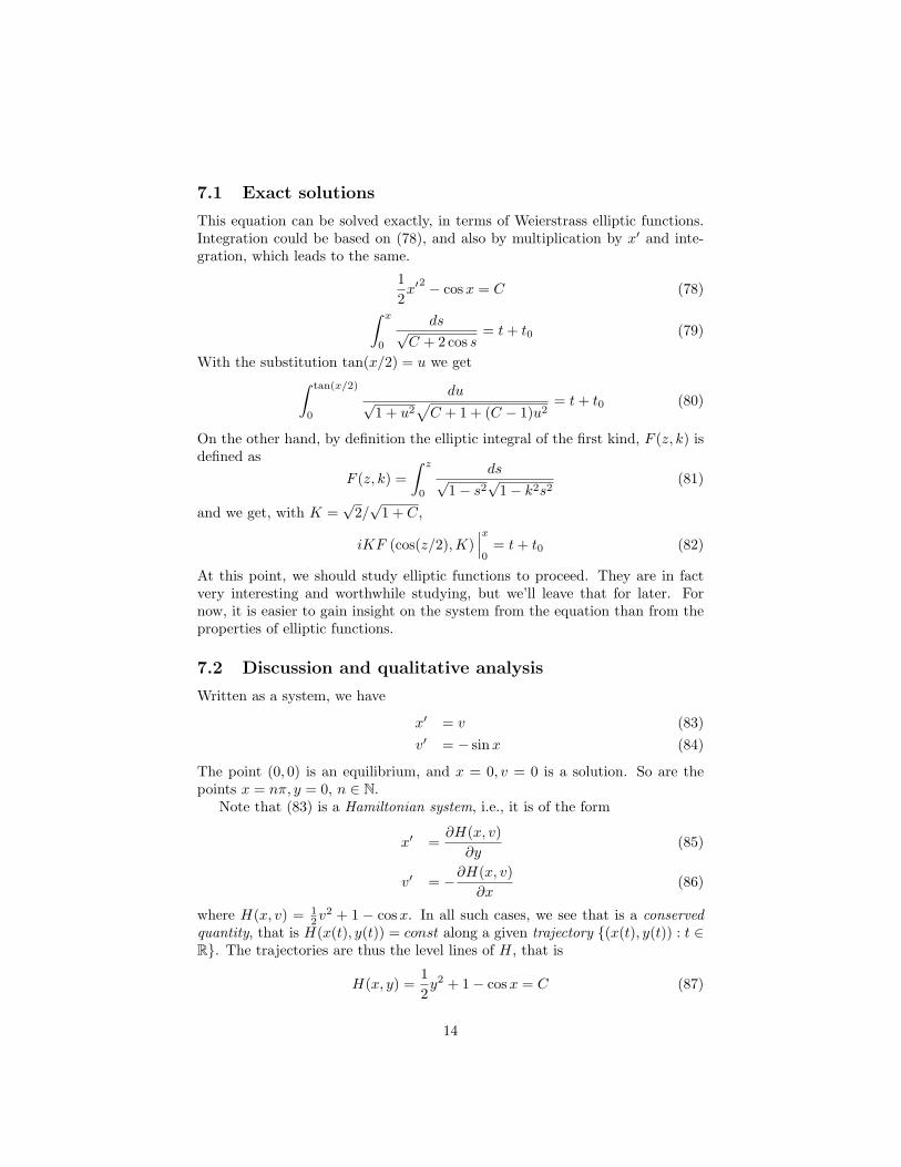
Fig. 8 represents a numerical contour plot of y2/2 − cos x. If we zoom in,we see that the program had difficulties at the critical points ±π, showing oncemore that there is something singular there.

7.3 Linearization of the phase portrait

Take(1− u2/2) = cosx; u ∈ [−2, 2] (90)

We can write this asu2 = 4 sin(x/2)2 (91)

which defines two holomorphic changes of coordinates

u = ±2 sin(x/2) (92)

These are indeed biholomorphic changes of variables until sin(x/2)′ = 0 that is,x = ±π. With any of these changes of coordinates we get

u

sin xu′ = v (93)

v′ = − sin x (94)

or

uu′ = v sin x (95)v′ = − sin x (96)

15

Figure 2: Contour plot of y2/2− cos x

which would give the same trajectories family as

u′ = v (97)v′ = −u (98)

for which the exact solution, A sin t, A cos t gives rise to circles. The same couldhave been seen easily seen by making the same substitution, (101) in (87). Wenote again that in (101) we have u2 ∈ [0, 4], so the equivalence does not holdbeyond u = ±2.

What about the other equilibria, x = (2k + 1)π? It is clear, by periodicityand symmetry that it suffices to look at x = π. If we make the change of variablex = π + s we get

s′ = v (99)v′ = sin s (100)

In this case, the same change of variable, u = 2 sin(s/2) gives

u′ = v (101)v′ = u (102)

16

implying v2−u2 = C as long as the change of variable is meaningful, that is, foru < 2, or |s| < π. So the curves associated to (99) are analytically conjugatedto the hyperbolas v2 − u2 = C. The equilibrium is unstable, points startingnearby necessarily moving far away. The point π, 0 is a saddle point.

The trajectories starting at π are heteroclinic: they link different saddles ofthe system. In general, they do not necessarily exist.

In our case, these trajectories correspond to H = 2 and this gives

v2 = 2(1 + cos(x)) (103)

orv2 = 4 cos(x/2)2 (104)

that is, the trajectories are given explicitly by

v = ±2 cos(x/2) (105)

This is a case where the elliptic function solution reduces to elementary func-tions: The equation

dx

dt= 2 cos(x/2) (106)

has the solutionx = 2arctan(sinh(t + C)) (107)

We see that the time needed to move from one saddle point to the next one isinfinite.

7.4 Connection to regularly perturbed equations

Note that at the equilibrium point (π, 0) the system of equations is analyticallyequivalent, insofar as trajectories go, to the system(

xv

)′=(

0 11 0

)(xv

)(108)

The eigenvalues of the matrix are ±1 with (unnormalized) eigenvectors (1, 1)and (−1, 1). Thus, the change of variables to bring the system to a diagonalform is x = ξ + η, v = ξ − η. We get

ξ′ + η′ = ξ − η (109)ξ′ − η′ = ξ + η (110)

By adding and subtracting these equations we get the diagonal form

ξ′ = ξ (111)η′ = −η (112)

ordξ

dη= − ξ

η; or ξη +

1ηξ = 0 (113)

17

a standard regularly perturbed equation. Clearly the solutions of (113) areξ = C/η with C ∈ (−∞,∞), and insofar as the phase portrait goes, we couldhave written ηξ + 1

ξ η = 0, which means that the trajectories are the curvesξ = C/η with C ∈ [−∞,∞], hyperbolas and the coordinate axes. In the originalvariables, the whole picture is rotated by 45◦.

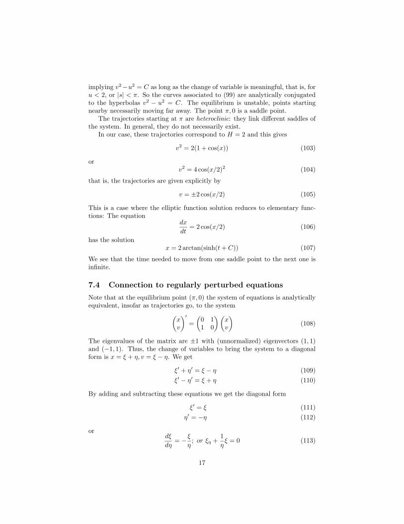
7.5 Completing the phase portrait

We see that, for H > 2 we have

v = ±√

2h + 2 cos(x) (114)

where now h > 2. With one choice of branch of the square root (the solutions areanalytic, after all), we see that |v| is bounded, and it is an open curve, definedon the whole of R. Note that the explicit form of the trajectories, given by(87) does not, in general, mean that we can solve the second order differentialequation. The way the pendulum position depends on time, or the way thepoint moves along these trajectories, is still transcendental.

Figure 3: Contour plot of y2/2− cos x

7.6 Local and asymptotic analysis

Near the origin, for C = a2 small, we have

x′ = v (115)v′ = x− x3/6 + ... (116)

implying

x′ = v (117)v′ ≈ x (118)

18

which means

x ≈ a sin t (119)v ≈ a cos t (120)

For C very large, we have

dx√C + cos x

= dx(C + cos x)−1/2 = dxC−1/2(1 + cos x/C)−1/2

= dx(C−1/2 − 12

cos x/C−3/2 + · · · ) (121)

which meansC−1/2x +

12

sin x/C−3/2 + · · · = t + t0 (122)

orx = C1/2(t + t0)−

12

sin(C1/2t)/C−3/2 + · · · = (123)

The solutions near the critical point (π, 0) can be analyzed similarly.Local and asymptotic analysis often give sufficient qualitative, and some-

times quantitative information about all solutions of the equation.

8 Equilibria, more examples and results

8.1 Flows

Consider the systemdx

dt= X(x) (124)

where X is smooth enough. Such equations can be considered in Rn or, moregenerally, in Banach spaces.

The initial condition x0 is mapped, by the solution of the differential equation(124) into x(t) where t ∈ (−a, b).

The map x(0) → x(t) written as f t(x0) is the flow associated to X.For t ≥ 0 we note the semigroup property f0 = I, fs+t = fsf t.

Fixed points, hyperbolic fixed points in Rn. Example. If X(x) = Bxwhere B does not depend on x, then the general solution is

x = eBtx0 (125)

where x0 is the initial condition at t = 0. (Note again that a simple exponentialformula does not exist, in general, if M depended on t.)

In this case, the flow f is given by the linear map

f t(x0) = eBtx0 (126)

Note that (Dxf)(0) = eBt. This is the case in general, as we will see.

19

Note 1. Check also (for instance from the power series of the exponential) thatthe eigenvalues of eBα are eλiα where λi are the eigenvalues of B.

Definition 5. The point x0 is a fixed point of f if f t(x0) = x0 for all t.

Proposition 6. If f is associated to X, then x0 is a fixed point of f iff X(x0) =0.

Proof. Indeed, we have x(t + ∆t) = x(t) + X(x0)∆t + O((∆t)2) for small ∆t.Then x(t + ∆t) = x(t) implies X(x0) + O(∆t) = 0, or, X(x0) = O(∆t), that is,X(x0) = 0. Conversely, it is obvious that X(x0) = 0 implies that x(t) = x0 is asolution of (124).

Proposition 7. If f is associated to X, and 0 is a fixed point of f , thenDxf t|x=0 = eDX(0)t.

Proof. Let t be fixed and take x0 small enough. Let DX(0) = B. We havex′ = Bx + O(x2), and thus, by taking x = eBtu we get

eBtu′ + BeBtu = BeBtu + g(eBtu) (127)

where g(s) = O(s2). Thus

u = x0 + e−Bt

∫ t

0

g(eBsu(s))ds (128)

We can check that for given t and x0 small enough, this equation is contractivein the sup norm, in the ball |u| < 2x0. Then, we see that

u = u0 + O(C(t)u20) (129)

where we emphasized that the correction depends on t too. Then,

x = eBtx0 + O(C(t)x20) (130)

proving the statement.

Definition 8. • The fixed point x = 0 is hyperbolic if the matrix Dxf |x=0 hasno eigenvalue on the unit circle.

• Equivalently, if f is associated with X, the fixed point 0 is hyperbolic if thematrix DX(0) has no purely imaginary eigenvalues.

8.2 The Hartman-Grobman theorem

The following result generalizes to Banach space settings.Let U and V be open subsets of Rn. Let f be a diffeomorphism between

U and V with a hyperbolic fixed point, that is there is x ∈ U ∩ V so thatf(x) = x. Without loss of generality, we may assume that x = 0.

20

Theorem 5 (Hartman-Grobman for maps). Under these assumptions, f andDf(0) are topologically conjugate, that is, there are neighborhoods U1, V1 of zero,and a homeomorphism h from U1 to V1 so that h−1 ◦ f ◦ h = Df(0).

The proof is not very difficult, but it is preferable to leave it for later.

Theorem 6 (Hartman-Grobman for flows, [5]). Let consider x′ = X(t) overa Banach space, where X is a C1 vector field defined in a neighborhood of theorigin 0 of E. Suppose that 0 is a hyperbolic fixed point of the flow described byX. Then there is a homeomorphism between the flows of X and DX(0), that isa homeomorphism between a neighborhood of zero into itself so that

f t = h ◦ etDX(0) ◦ h−1 (131)

See also [4].The more regularity is needed, the more conditions are required.

Differentiable linearizations

Theorem 7 (Sternberg-Siegel, see [5]). Assume f is differentiable, with a hy-perbolic fixed point at zero, and the derivative Df is Holder continuous nearzero. Assume further that DX(0) is such that its eigenvalues satisfy

Reλi 6= Reλj + Reλk (132)

when Reλj < 0 < Reλk. Then the functions h in Theorems 5 and 6 can betaken to be diffeomorphisms.

Smooth linearizations

Theorem 8 (Sternberg-Siegel, see [5]). Assume f ∈ C∞ and the eigenvaluesof Df(0) are nonresonant, that is

λi − kλ 6= 0 (133)

for any k with |k| > 1. Then the functions h in Theorems 5 and 6 can be takento be C∞ diffeomorphisms.

We will prove, in simpler settings, the Hartman-Grobman theorem for flows.

For the analytic case, see Proposition 3.

8.3 Bifurcations

Bifurcations occur in systems depending on a parameter (or more), call it s.Thus, the system is

d

dtx(t; s) = X(x; s) (134)

A local bifurcation at an equilibrium, say x = 0, X(0) = 0, may occur when atleast one of the eigenvalues of DX(0) becomes purely imaginary. (Otherwise,

21

the linearization theorem shows that the phase portrait is locally similar to thatof the linearized system. In this case, the topology does not change unless weindeed go through purely imaginary eigenvalues.) We will explore bifurcationtypes and prove theorems about some of them, but before that let’s see whattypes of equilibria are possible in linear systems. Those that are associated tohyperbolic fields represent, again by the linearization theorem, the local behaviorof general hyperbolic systems.

9 Types of equilibria of linear systems with con-stant coefficients in 2d

The equation is nowx′ = Bx (135)

where B is a 2× 2 matrix with constant coefficients.

9.1 Distinct eigenvalues

In this case, the system can be diagonalized, and it is equivalent to a pair oftrivial first order ODEs

x′ = λ1x (136)y′ = λ2y (137)

9.1.1 Real eigenvalues

The change of variables that diagonalizes the system has the effect of rotatingand rescaling the phase portrait of (136). The phase portrait of (136) can befully described, since we can solve the system in closed form, in terms of simplefunctions:

x = x0eλ1t (138)

y = y0eλ2t (139)

On the other hand, we have

dy

dx=

λ2

λ1

y

x= a

y

x⇒ y = C|x|a (140)

where we also have as trajectories the coordinate axes: y = 0 (C = 0) and x = 0(”C = ∞”). These trajectories are generalized parabolas. If a > 0 then thesystem is either (i) a sink, when both λ’s are negative, in which case, clearly,the solutions converge to zero. See Fig. 4, or (ii) a source, when both λ’s arepositive, in which case, the solutions go to infinity.

The other case is that when a < 0; then the eigenvalues have oppositesign. Then, we are dealing with a saddle. The trajectories are generalizedhyperbolas,

y = C|x|−|a| (141)

22

Figure 4: All types of linear equilibria in 2d, modulo euclidian transformationsand rescalings: sink, source, spiral sink, saddle, nontrivial Jordan form, centerresp. In the last two cases, the arrows point according to the sign of λ or ω,resp.

23

Say λ1 > 0. In this case there is a stable manifold the y axis, along whichsolutions converge to zero, and an unstable manifold in which trajectories goto zero as t → −∞. Other trajectories go to infinity both forward and backwardin time. In the other case, λ1 < 0, the figure is essentially rotated by π/2.

9.1.2 Complex eigenvalues

In this case we just keep the system as is,

x′ = ax + by (142)y′ = cx + dy (143)

We solve for y, assuming b 6= 0 (check the case b = 0!), introduce in the secondequation and we obtain a second order, constant coefficient, differential equationfor x:

x′′ − (a + d)x′ + (ad− bc)x = 0 or (144)x′′ − tr(B)x′ + det(B)x = 0 (145)

If we substitute x = eλt in (144) we obtain

λ2 − tr(B)λ + det(B) = 0 (146)

and, evidently, since λ1 + λ2 = tr(B) and λ1λ2 = det(B), this is the sameequation as the one for the eigenvalues of B. The eigenvalues of B have beenassumed complex, and since the coefficients we are working with are real, theroots are complex conjugate:

λi = α± iω (147)

The real valued solutions are

x = Aeαt sin(ωt + ϕ) (148)

where A and ϕ are free constants. Substituting in

y = b−1x′ − ab−1x (149)

we gety(t) = Aeαtb−1[(α− 1) cos(ωt + ϕ)− ω sin(ωt + ϕ) (150)

which can be written, as usual,

y(t) = A1eαt sin(ωt + ϕ1) (151)

If λ < 0, then we get the spiral sink. If α > 0 then we get a spiral source,where the arrows are reverted.

A special case is that when α = 0. This is the only non-hyperbolic fixedpoint with distinct eigenvalues. In this case, show that for some c we havex2 +cy2 = A2, and thus the trajectories are ellipses. In this case, we are dealingwith a center.

24

9.2 Repeated eigenvalues

In 2d this case there is exactly one eigenvalue, and it must be real, since itcoincides with its complex conjugate. Then the system can be brought to aJordan normal form; this is either a diagonal matrix, in which case it is easy tosee that we are dealing with a sink or a source, or else we have(

xy

)′=(

λ 10 λ

)(xy

)(152)

In this case, we obtaindx

dy=

x

y+

1λ

(153)

with solutionx = ay + λ−1y ln |y| (154)

As a function of time, we can write

(xy

)= e

0@λ 10 λ

1At

= eλt[I +

(0 10 0

)t](x0

y0

)(155)

x(t) = (At + B)eλt (156)y(t) = Aeλt (157)

We see that, in this case, only the x axis is a special solution (the y axis is not),and thus, all solutions approach (as t → ∞ or t → −∞ for λ < 0 or λ > 0respectively) the x axis.

Note 2. The eigenvalues of a matrix depend continuously on the coefficients ofthe matrix. In two dimensions you can see this by directly solving λ2−Tr(A)λ+det(A) = 0. Thus, if a linear or nonlinear system depends on a parameter α(scalar or not) and the equilibrium is hyperbolic when α = α0, then the realpart of the eigenvalues will preserve their sign in a neighborhood of α = α0. Thetype of equilibrium is the same and of local phase portrait changes smoothlyunless the real part of an eigenvalue goes through zero.

Note 3. When conditions are met for a diffeomorphic local linearization at anequilibrium, then we have (

xy

)= ϕ

(uv

)(158)

where the equation in (u, v) is linear and the matrix ϕ is a diffeomorphism. Wethen have (

xy

)= (Dϕ)

(uv

)+ o(u, v) (159)

which implies, in particular that the phase portrait very near the equilibrium ischanged through a linear transformation.

25

9.3 Further examples, [4]

Consider the system

x′ = x + y2 (160)y′ = −y (161)

The linear part of this system is

x′ = x (162)y′ = −y (163)

The associated matrix is simply (1 00 −1

)(164)

with eigenvalues 1 and −1, and the conditions of a differentiable homeomor-phism are satisfied.

Locally, near zero, the phase portrait of the system (164) is thus the proto-typical saddle.

We will see that, again insofar as the field lines are concerned, this systemcan be globally linearized too.

How about the global behavior? In this case, we can completely solve thesystem. First, insofar as the field lines go, we have

dx

dy= −x

y+ y (165)

a linear inhomogeneous equation that can be solved by variation of parameters,or more easily noting that, by homogeneity, x = ay2 must be a particularsolution for some a, and we check that a = −1/3. The general solution of thehomogeneous equation is clearly xy = C. It is interesting to make it into ahomogeneous second order equation by the usual method. We write

1y

dx

dy= − x

y2+ 1 (166)

and differentiate once more to get

d2x

dy2= −2

x

y2(167)

which is an Euler equation, with indicial equation (λ− 2)(λ + 1) = 0, and thusthe general solution is

x(y) = ay2 +b

y(168)

where the constants are not arbitrary yet, since we have to solve the morestringent equation (165). Inserting (168) into (165) we get a = −1/3. Thus, thegeneral solution of (166) is

3xy + y3 = C (169)

26

Figure 5: Phase portrait of (160)

which can be, of course, solved for x. The phase can be obtained in the followingway: we note that near the origin, the system is diffeomorphic to the linear part,thus we have a saddle there. There is a particular solution with x = −1/3y2

and the field can be completed by analyzing the field for large x and y. Thisseparates the initial conditions for which the solution ends up in the right halfplane from those confined to the left half plane.

Global linearization. This is another case of “accidental” analytic lin-earizability since we can write the conserved quantity 3xy(1+ y2/3) = C, whichor (x + y2/3)y = C and thus passing to the variables u = x + y2/3, v = y thesystem (160) becomes linear, of the form (162) (check!)

Note 4. The change of coordinates is thus(uv

)=(

I +(

0 y2/30 0

))(xy

)(170)

and in particular we see that the transformation is, to leading order, the identity.

Exact solution of the time dependent system. Due to the very specialnature of the equation, an exact solution is possible too: we note that the secondequation contains y alone, and it gives immediately

y = y(0)e−t

while x can be either solved from the first equation or, more simply, from (176):

x(t) =c

y(0)et − 1

3y(0)e−2t (171)

In the nonlinear system, y = 0 is still a solution, but x = 0 is not; x = 0 is“deformed” into the parabola x = (−1/3)y2.

27

9.4 Stable and unstable manifolds in 2d

Assume that ϕ is differentiable, and that the system(xy

)′= ϕ

(xy

)(172)

has an equilibrium at zero, which is a saddle, that is, the eigenvalues of (Dϕ)(0)are −µ and λ, where λ and µ are positive. We can make a linear change ofvariables so that (Dϕ)(0) = diag(−µ, λ). Consider the linearization tangent tothe identity, that is, with Dϕ(0) = I. We call the linearized variables (u, v).

Theorem 9. Under these assumptions, in a disk of radius ε > 0 near the originthere exist two functions y = f+(x) and x = f−(y) passing through the origin,tangent to the axes at the origin and so that all solutions with initial conditions(x0, f+(x0)) converge to zero as t →∞, while the initial conditions (f−(y0), y0)converge to zero as t → −∞. The graphs of these functions are called the stableand unstable manifolds, resp. All other initial conditions necessarily leavethis disk as time increases, or decreases.

Proof. We show the existence of the curve f+, the proof for f− being the same,by reverting the signs. We have

x(t) = ϕ1(u(t), v(t))y(t) = ϕ2(u(t), v(t)) (173)

Consider a point (ϕ1(u0, 0), ϕ2(u0, 0)). There is a unique solution passingthrough this point, namely (ϕ1(u+(t), 0), ϕ2(0+(t), 0)) where u+(0) = u0, v+(0) =0. Since u+(t) → 0 as t →∞ and ϕ is continuous, we have

(ϕ1(u+(t), 0), ϕ2(u+(t), 0)) → 0

as t → ∞. Since ϕ = I + o(1), we have ∂ϕ2/∂y = 1 at (0, 0), and the implicitfunction theorem shows that ϕ2(x, y) = 0 defines a differentiable function y =f(x) near zero, and y′(0) = 0 (check). For other solutions we have, from (173),that x, y exits any small enough disk (check).

9.5 A limit cycle

We follow again [4], but with a different starting point. Let’s look at the simplesystem

r′ = r(1− r2)/2 (174)θ′ = 1 (175)

Obviously, we can solve this in closed form. The flow clearly has no fixed point,since the field never vanishes. To solve the first equation, note that if we multiplyby 2r we get

2rr′ = r2(1− r2) (176)

28

or, with u = r2,u′ = u(1− u) (177)

The exact solution is

r = ±(1 + Ce−t)−1/2; or r = 0; ±1 are special constant solutions (178)θ = t + t0 (179)

We see that all solutions that start away from zero converge to one as t → ∞.What if interpret r and θ as polar coordinates and write the equations for x

Figure 6: Phase portrait of (174)

and y? We get

x′ = r′ cos θ − r sin θθ′ =12r(1− r2) cos θ − r sin θ

=12x− y − 1

2(x3 + xy2) (180)

y′ = r′ sin θ + r cos θθ′ =12r(1− r2) sin θ + r cos θ

= x +12y − 1

2(x2y + y3) (181)

thus the system

x′ =12x− y − 1

2(x3 + xy2) (182)

y′ = x +12y − 1

2(x2y + y3) (183)

which looks rather hopeless, but we know that it can be solved in closed form.

29

To analyze this system, we see first that at the origin the matrix is(12 −11 1

2

)(184)

with eigenvalues 1/2± i. Thus the origin is a spiral source. There are no otherequilibria (why?)

Now we know the solution globally, by looking at the solution of (174) and/orits phase portrait. We note that r = 1 is a solution of (174), thus the unit circle

Figure 7: Phase portrait of (174)

is a trajectory of the system (182). It is a closed curve, all trajectories tend toit asymptotically. This is a limit cycle.

9.6 Application: constant real part, imaginary part of an-alytic functions

Assume for simplicity that f is entire. The transformation z → f(z) is associ-ated with the planar transformation (x, y) → (u(x, y), v(x, y)) where f = u+ iv.The grid x = const, y = const is transformed into the grid u = const, v = const.We can first look at what this latter grid is transformed back into, by the trans-formation. The analysis is more general though, nothing below requires u + ivto be analytic. We use only use this information to shortcut through somecalculations.

30

We take first u(x(t), y(t)) = const. We have

∂u

∂xx′(t) +

∂u

∂yy′(t) = 0 (185)

which we can write, for instance, as the system

x′ =∂u

∂y(186)

y′ = −∂u

∂x(187)

which, in particular, is a Hamiltonian system. We have a similar system forv. We can draw the curves u = const, v = const either by solving this implicitequation, or by analyzing (186), or even better, by combining the informationfrom both. Let’s take, for example f(z) = z3− 3z2. Then, v = 3x2y− y3− 6xy.It would be rather awkward to solve v = c for either x or y. The system ofequations reads

x′ = −6x + 3x2 − 3y2 (188)y′ = 6y − 6xy (189)

Note that ∇u = 0 or ∇v = 0 are equivalent to z′ = 0. For equilibria, we thussolve 3z2 − 6z = 0 which gives z = 0; z = 2. Near z = 0 we have

Figure 8: Phase portrait of (188) near (0, 0).

x′ = −6x + o(x, y) (190)y′ = 6y + o(x, y) (191)

31

which is clearly a saddle point, with x the stable direction and y the unstableone. At x = 2, y = 0 we have, denoting x = 2 + s,

s′ = 6s + o(s, y) (192)y′ = −6y + o(s, y) (193)

another saddle, where now y = 0 is the unstable direction. We note that y = 0 is,

Figure 9: Phase portrait of (188) near (0, 2).

in fact, a special trajectory, and it is in the nonlinear unstable/stable manifoldat the equilibrium points. Note also that a nonlinear stable manifold existslocally. In this case it changes character as it happens to pass through anotherequilibrium.

We draw the phase portraits near x = 0, near x = 2, mark the specialtrajectory, and look at the behavior of the phase portrait at infinity. Then we“link” smoothly the phase portraits at the special points, and this should sufficefor having the phase portrait of the whole system.

For the behavior at infinity, we note that if we write

dy

dx=

y(1− 6x)−6x + 3x2 − 3y2

(194)

we have the special solution y = 0, and otherwise the nonlinear terms dominateand we have

dy

dx≈ −6yx

3x2 − 3y2(195)

By homogeneity, we look for special solutions of the form y = ax (which would

32

be asymptotes for the various branches of y(x). We get, to leading order,

a =−6a

3− 3a2(196)

We obtaina = 0, a = ±

√3 (197)

We also see that, if x = o(y), then y′ = o(1) as well. This would give usinformation about the whole phase portrait, at least qualitatively.

Figure 10: Phase portrait of (188), v = const.

Exercise 1. Analyze the phase portrait of u(x, y) = const.

The two phase portraits, plotted together give Note how the fields intersectat right angles, except at the saddle points. The reason, of course, is that f(z)is a conformal mapping wherever f ′ 6= 0.

33

Figure 11: Phase portrait of u = const

Figure 12: Phase portrait of u = const, and v = const.

References

[1] E.A. Coddington and N. Levinson, Theory of Ordinary Differential Equa-tions, McGraw-Hill, New York, (1955).

[2] R.D. Costin, Nonlinear perturbations of Fuchsian systems, Nonlinearity 9,

34

pp. 2073–2082 (2008).

[3] J. Ecalle and B. Valet Correction and linearization of resonant vector fieldsand diffeomorphisms, Mathematische Zeitschrift, 229, 2, pp. 249–318 (1998)

[4] M.W.Hirsch, S. Smale and R.L. Devaney, Differential Equations, Dynami-cal Systems & An Introduction to Chaos, Academic Press, New York (2004).

[5] D. Ruelle, Elements of Differentiable Dynamics and Bifurcation theory,Academic Press, Ney York , (1989)

35