1. Principles of VPE

Virtual Plankton Ecology by Woods & Vallerga - 11 -

VIRTUAL PLANKTON ECOLOGY CH.1.docx Last printed 27/08/2009 09:36

1 Principles of Virtual Plankton Ecology

Contents

1.1 Modelling in biological oceanography

1.2 Quantifying complexity 1.3 Philosophy of virtual ecology

1.4 Primitive equation modelling 1.5 The Lagrangian Ensemble metamodel

1.6 External forcing 1.7 Integration

1.8 The virtual ecosystem 1.9 Intra-population variability

1.10 Emergent demography and biofeedback 1.11 Information flow from DNA to Prediction

1.12 Comparison with population-based modelling 1.13 Scientific analysis

1.14 Prediction 1.15 Error analysis and control

1.16 Comparison with observations 1.17 Virtual Ecology Workbench

1.18 Conclusion



1.1 Modelling in biological oceanography

Biological oceanographers are ambivalent about modelling (Miller 2004). Many are

concerned that mathematical simulation over-simplifies the natural plankton

ecosystem. That is not contested. However modelling can still contribute to biological

oceanography. The goal of this book is to justify that claim. It does so in two ways.

1. By establishing the scientific integrity of a new method for mathematical

simulation called Virtual Plankton Ecology. Theory and practice are presented

in Parts 1 and 2 respectively.

2. By demonstrating how this new method can contribute to biological

oceanography. This is done in Part 3 by using virtual ecology to investigate

the classical paradigms of biological oceanography. The proof of the pudding

lies in the eating.

Chapter 1 opens the discussion on the first theme: scientific integrity. It introduces the

key ideas of virtual plankton ecology. It is like the overture of an opera, which brings

together themes that will be developed in full later. It presents in brief form the pre-

requisites for best practice in modelling the plankton ecosystem. They are the

Principles of Virtual Ecology.

But first we need to address the issue of over-simplification, which causes biological

oceanographers to worry about the value of modelling, even when performed well. To

do so we quantify the complexity of first the natural ecosystem and then a typical

virtual ecosystem.

1.2 Quantifying complexity

We compare the information contents of natural and simulated ecosystems, both

located in mid-ocean off the Azores. They are contained in a water column that has

the form of a vertical tube extending from the sea surface to a depth of one kilometre

with a horizontal cross-section of one square metre. They are both computationally

complex.3 Their descriptions of the environment contain about the same information.

3 Computational complexity is an expression used by information theorists to describe the inherent complexity of a system (Traub, J. F. and A. G. Werschulz (1998). Complexity and



The difference lies in the number of plankters and, more importantly, in the number of

species.

1.2.1 The natural ecosystem

We divide the ecosystem into two parts: the environment and the plankton. The

physical environment can be described by vertical profiles of solar radiation,

temperature, density, horizontal currents, upwelling and turbulence. These profiles all

contain fine structure that is ecologically important. The spectrum of this fine

structure extends to about one decimeter. The same is true for the profiles of dissolved

chemical concentrations. The spectral limit is set by molecular conduction and

diffusion. We may need to include the profiles of ten or more dissolved chemicals. So

a synoptic description of the physical and chemical properties of the environment in

the mesoscosm requires about one million values.

But the complexity of the environment is tiny compared with that of the plankton.

(Miller 2004) and (Longhurst 1998) estimate that a thousand species of plankton

might be encountered in the water column.4 The same authors estimate the minimum

number of plankters in one thousand cubic metres of our water column: 105

macroplankters and 1015 bacteria. The numbers vary seasonally. And the distribution

of plankton in the ocean is observed to be patchy with two orders of magnitude

variation in concentration within a 100km area. But the values cited above will serve

our purpose of highlighting the difference in complexity between natural and

simulated ecosystems.

1.2.2 The virtual ecosystem

Now we assess the complexity of a virtual ecosystem in the same water column off

the Azores. The data come from the case study in chapter 10. The environmental

fields are resolved to one-metre, which is an order of magnitude coarser than the fine

structure in the natural ecosystem. However it is feasible to increase the vertical

information. Cambridge, Cambridge University Press.). It does not refer to the efficiency of a computer program used to model the system, although we shall see later that VPE codes are indeed complex (Chapter 7). 4 One plankton net tow can sample the 1000 m3 volume of the water column used in this discussion, but it may take many tows at the same site to encounter all 1000 species.



resolution to match that in nature. So the difference in complexity does not depend

critically on how the environment is modelled.

The plankton are described by computer agents, each of which follows an

independent trajectory through the water and carries two kinds of information. The

first describes the number of identical plankters in its sub-population. The second

describes the biological state of those plankters. The virtual ecosystem in chapter 10

uses about one million agents. Summing the sub-populations gives the total number of

plankters in the water column. That sum is performed separately for each species. The

number of agents determines the demographic complexity of the simulation. It is three

orders of magnitude less than the number of plankters in the natural ecosystem.

However, we shall see in chapter two that this is not a limiting factor, provided the

number of agents is sufficient to simulate the statistics of intra-population variability

with an acceptable signal-to-noise ratio.

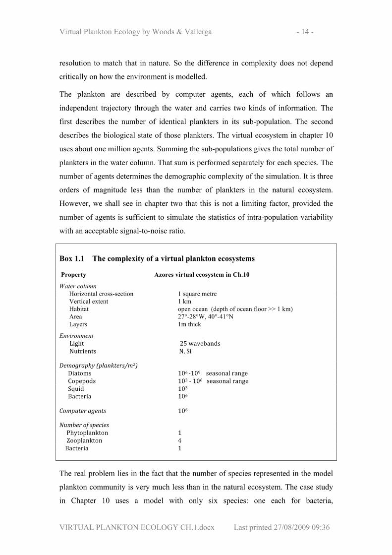
Box 1.1 The complexity of a virtual plankton ecosystems

Property Azores virtual ecosystem in Ch.10

Water column Horizontal cross-section 1 square metre Vertical extent 1 km Habitat open ocean (depth of ocean floor >> 1 km) Area 27°-28°W, 40°-41°N Layers 1m thick

Environment Light 25 wavebands Nutrients N, Si

Demography (plankters/m2) Diatoms 106 ‐109 seasonal range Copepods 103 ‐ 106 seasonal range Squid 103 Bacteria 106

Computer agents 106

Number of species Phytoplankton 1 Zooplankton 4 Bacteria 1

The real problem lies in the fact that the number of species represented in the model

plankton community is very much less than in the natural ecosystem. The case study

in Chapter 10 uses a model with only six species: one each for bacteria,



phytoplankton, herbivorous and carnivorous zooplankton, and two for top predators.

More species are used in the numerical experiments reported in other chapters. For

example, chapter 18 models competition between 16 species of phytoplankton.

However, in all the simulations described in this book the number of model species is

orders of magnitude lower than those observed in the natural ecosystem. As modellers

gain access to more powerful computers they will be able to create models with more

species, but it is unlikely that the diversity gap between model and reality will ever be

closed. That is true regardless of the metamodel used to generate the simulation.

Classical population-based modelling (PBM) is computationally cheaper than agent-

based modelling like VPE. But even complex PB models like ERSEM (Baretta-

Bekker and Baretta 1997) uses only 16 species.

1.2.3 The way ahead

It is this diversity gap that leads biological oceanographers to doubt the value of

computer simulation. There is no procedure that can close it. The usual compromise is

to design model plankton communities that minimize the impact of inadequate

diversity. They can do so by concentrating on the most abundant species, and adding

functional groups to represent the remaining species. We shall explore these options

in Chapter 6. It goes without saying that the modelling procedure must avoid

unnecessary loss of information, for example neglecting intra-population variability

(see §1.9 below). Whatever the procedure, the model complexity will always be

woefully inadequate when it comes to species diversity.

However, that does not necessarily mean that computer simulation has no value. It

means that we have to demonstrate its value by comparison with the results of

observations (see §1.16 below). There will always be a diversity gap, but we shall

show that many of the predictions of virtual ecosystems are not particularly sensitive

to that shortcoming.

1.2.4 Sensitivity of predictions to species diversity

In general, we expect some ecological predictions to be more sensitive than others to

a lack of species diversity. For example, the numerical experiment of (Liu and Woods

2004) showed that increasing the number of phytoplankton species from one to three

eliminated the gap between predicted and observed timing of the annual maximum



perturbation of ocean colour, a surrogate for the annual maximum concentration of

chlorophyll in the mixed layer (see below §1.16.9). That procedure might be applied

to other ecological phenomena identified in virtual ecosystems. In each case the

sensitivity to species diversity can be assessed by a batch of experiments with

progressively increasing diversity. We expect that the benefit of adding more species

to the model will eventually decrease until it becomes lost in the noise of those

properties used to define the phenomenon. They are normally time series of the values

of environmental fields. Furthermore, adding more species to the model becomes

redundant when the gap is closed between prediction and observation of those

defining properties.

When the biological model includes sufficient species for the VE to pass the

Ecological Turing Test (see §1.16 below) we are confident that the VE simulation of

this particular ecological phenomenon is not contaminated by lack of species

diversity. Following this procedure we can rank the various ecological phenomena in

terms of their sensitivity to species diversity. That will guide us in deciding how many

species are needed to qualify an ecological phenomenon for analysis by virtual

ecology. We can then use the power of audit trails to improve understanding of these

ecological phenomena. The procedure is demonstrated in Part 3, where we use virtual

ecology to re-examine classical paradigms of biological oceanography. Part 4 goes

further by considering how qualifying ecological phenomena might provide a secure

basis for prediction in operational oceanography. In conclusion, while all models of

the plankton ecosystem have many fewer species than in nature, we have a rational

procedure for discovering how many species are needed in a virtual ecosystem for it

to make predictions that are useful for biological and operational oceanography.

1.2.5 Success with other complex systems

One reason for being cautiously optimistic is that mathematical simulations of many

other complex systems do yield useful predictions. That is the case in weather

forecasting, ocean circulation and climate prediction. The same approach is used in an

increasing range of engineering applications. It is becoming normal practice to rely on

mathematical simulation rather than live action. Examples include virtual tests of

nuclear bombs, aero-engines and motorcar crashes. Models based on quantum

mechanics are used to design complicated molecules needed by the pharmaceutical



industry. Licensing authorities increasingly accept the evidence of mathematical

simulation. Pilots can obtain licences to fly new planes by demonstrating their skills

on simulators.

Most of these practical applications of mathematical simulation of complex systems

use equations that describe the laws of physics.5 In this chapter we explore the

prospect for extending this approach to the plankton ecosystem. This requires multi-

disciplinary models comprising equations for processes in marine physics, chemistry

and biology. The main challenge is to describe the biological processes of plankton.

1.2.6 Complexity science

A new scientific discipline, complexity science, has been built on these practical

applications of mathematical simulation on high performance computers. Initially

applications tended to focus on models with physical equations, but scientists at the

Santa Fe institute and elsewhere have extended the subject into the world of social

sciences, economics and business (Waldrop 1992). They have published SWARM, a

rich library of computer routines designed to ease building models of complex

systems. SWARM is particularly effective in rapid prototyping. Woods et al (2007)

used it for Container World, which simulates the global freight system. (Grimm and

Railsback 2005) used SWARM to model ecosystems. McLane (2001) used it to build

an individual-based model of the plankton ecosystem. But SWARM is cumbersome

and slow. Projects needing many numerical experiments are better written in purpose-

build code. Java is well suited to agent-based modelling. It runs on any personal

computer with a Java compiler. Container World was re-written in Java. The Virtual

Ecology Workbench is written in Java and it automatically writes runtime code in

Java (§1.16).

We now have a broad theoretical understanding of complex system simulations. Let

us mention two examples. The first concerns the nature of stability in complex

systems. Many are chaotic with limited predictability; they are described by strange

attractors (Lorenz 1993). There has been a lively debate about whether or not the

plankton ecosystem is intrinsically chaotic in a way that would place a limit on

5 In this book we define a model as a set of equations, and a simulation as the data set that results from integrating the model with prescribed initial and boundary conditions.



prediction, like the one-week limit on weather forecasting (see references cited in

Woods et al. 2005). The second example concerns optimal procedures for

assimilating observations into simulations (Lorenc 2002); we shall discuss this below

(§1.14). This new understanding helps us to simulating the plankton ecosystem,

which is even more complex than the examples mentioned above. It will inform the

discussions throughout this book; and it is highlighted in chapter 8 (stability) and

chapters 10 and 32 (observations and predictions). The success of complexity science

depends on adopting a metamodel drawn from physics to address inter-disciplinary

problems. Virtual ecology uses the Lagrangian Ensemble metamodel (Ch.2).

1.3 The philosophy of virtual plankton ecology

Now we turn to the main theme of this chapter, the unique features of VPE that make

it different from other modelling techniques. Some techniques concentrate on a single

ecological process. They follow Occam’s razor and eliminate all other processes. A

well-known early example is (Sverdrup 1953)’s model of the spring bloom. Others

provide basic biological functions in operational oceanography. A recent example is

the NOCS-Met. Office Medusa model (New 2009).

VPE is designed to provide theoretical support for biological oceanography. It

produces simulations, Virtual Ecosystems (VEs), that are very much more complex

than those created by other methods. The extra complexity allows each VE to include

many interacting ecological processes. The aim is to create realistic simulations. Two

aspects require further attention:

• The present generation of VEs are one-dimensional and therefore do not

simulate the patchiness created by mesoscale turbulence. This deficiency is

being addressed (see Ch. 30).

• Virtual ecosystems have a much smaller number of species than are found at

the same site in the ocean. They typically have about 1% of the macro-

plankton species, and a much smaller fraction of the bacteria. However many

ecological processes are insensitive to species diversity (§1.2.4 above) and the

deficiency can be dealt by a modest increase in the number of species.



VPE is an extended version of individual-based modelling (Grimm and Railsback

2005). It simulates the life history of every plankter in the ecosystem contained in a

virtual mesocosm. That information is used to compute the demography of each

population, and its influence on the environment (biofeedback). That is the

quintessence of VPE. However its success depends on having rethought all aspects of

plankton ecology modelling.

The philosophy of VPE is not merely an extension of previous modelling practice. It

has been built up from first principles, from a tabula rasa. The result is a distinct

approach to every aspect of the subject. In some cases VPE practice echoes classical

modelling, but in others it is new. A notable example is the emphasis on assessing and

controlling errors in emergent properties. That leads to a new way to compare model

predictions with observations. Another example is the need to balance a virtual

ecosystem, so that it settles on a stable attractor, before embarking on scientific

analysis. That changes the practice of data assimilation and prediction.

This philosophy has but one aim. It is to ensure that VPE is fit for purpose: that it is a

reliable tool in theoretical plankton ecology, and therefore useful for biological

oceanography. This demands scientific integrity. The philosophy will be explored in

detail in the next ten chapters. The rest of this opening chapter will be devoted to a

quick overview to show the scope of the philosophy before getting into detail. The

topics selected for treatment here all contribute to making the new method

trustworthy. Together they constitute the principles of virtual plankton ecology.

1.4 Primitive equation modelling

We start by identifying one of the principal differences between virtual ecology and

other methods used to simulate the plankton ecosystem. It concerns the nature of the

equations used to describe physical, chemical and biological processes in the

ecosystem. These equations make up the model. The goal of VPE is to base the

equations on the results of reproducible experiments performed under laboratory

conditions. If that can be achieved the virtual ecosystem created by integrating the

model under the conditions of external forcing will have secure scientific foundations.

Modern weather forecasting depends on using such equations for physical processes

in the atmosphere. Meteorologists call them “primitive equations”, and refer to



primitive equation modelling.6 Virtual plankton ecology depends on using primitive

equations for biological as well as physical and chemical processes (Woods 2002).

1.4.1 Biological primitive equations

What are biological primitive equations? They describe the physiological or

behavioural response of a plankter to the combination of (1) its own biological state,

and (2) the environment at its location. The latter is called the plankter’s ambient

environment. It is defined as the values that all the environmental fields7 have at its

precise location (latitude, longitude and depth) at a given time. Such equations are

called phenotypic. Phenotypic equations are derived by curve fitting to the results of

reproducible experiments with plankton cultures. That gives them the same scientific

stature as physical primitive equations.

1.4.2 Individual‐based modelling

Phenotypic equations describe the biological functions of an individual plankter. It

follows that primitive equation modelling of the plankton ecosystem must adopt the

procedures of individual-based modelling (DeAngelis and Gross 1992), (McGlade

1999), (Grimm and Railsback 2005). The aim is to compute the life history of every

plankter in the virtual ecosystem. Each plankter responds to its ambient environment,

which has physical, chemical and biological components. The ambient biological

environment is determined by the concentration of predators and prey in the

plankter’s immediate vicinity. The local concentration of competitors of the same or

different species influences the rates of depletion of shared resources. The response to

predators often involves avoidance reaction (Kiørboe 2008). The response to prey

involves foraging, capture and ingestion. These behavioural responses are described

by phenotypic equations in the model. Other phenotypic equations describe the

plankter’s physiological response to ingestion of prey (by zooplankters) or uptake of

nutrients and light (by phytoplankters). These equations are discussed in chapter 6.

6 Primitive equations in physics go back to Galileo’s investigation of acceleration. 7 The fields describe the continuous variation of environment properties like solar irradiance, seawater temperature, chemical concentrations, and turbulent kinetic energy. They also include the concentration of each species of plankton present in the virtual ecosystem. In most cases, the plankton concentrations are categorized by the biological state, which includes growth stage of living plankton, the corpses of dead plankton and fæcal pellets of zooplankton.



1.4.3 Phenotypic rules

Phenotypic equations are normally published as differential equations, implying that a

plankter responds continuously to its ambient environment. In fact many biological

processes are better described in terms of discrete events. There may be one or more

such event in one time step of numerical integration. Reproduction and

metamorphosis between growth stages are examples of biological events that are

likely to occur only once in a half-hour time step. Other processes involve several

events in one time step; for example, a plankter captures and ingests a number of prey

in half an hour. Event-based biological processes are often better described by rules

rather than differential equations. Inward looking rules state how to compute the new

location or physiological state of a plankter. Outward looking rules describe the

plankter’s impact on the environment. This biological requirement is consistent with

expressing differential equations in finite difference form for numerical integration. In

their textbook on individual-based modelling (Grimm and Railsback 2005)

recommend that biological functions should be expressed as rules rather than

equations. The typical imperative in biology is not “Thou shalt ….” but “If … then

… else … (Pinker 1997). So the phenotypic rule is often expressed as a Boolean

statement. That practice is followed in virtual plankton ecology. The graphical

interface of the Virtual Ecology Workbench makes it easy to enter biological

functions in terms of such rules (Ch.7).

1.5 The Lagrangian Ensemble metamodel

Individual-based models are integrated by a technique developed in computer science

called agent-based modelling (Billari, Fent et al. 2006). Each plankter is associated

with a computer agent. The computation focuses on the changing properties of the

agents. The final data set contains the life history of every agent, and the plankter it

represents. (Grimm and Railsback 2005) describe how that procedure can be used to

simulate ecosystems. It works well if the number of organisms in the ecosystem does

not exceed the number of agents that can be computed. Modern computers can

integrate models with several hundred thousand agents per processor. A dual-core

laptop computer with two gigabytes of memory can simulate an ecosystem with

approaching one million agents. That might suffice for modelling all the trees in a



wood. But it is inadequate for handling the plankton ecosystem in a mesoscosm

containing one thousand cubic metres of water. There may be a billion

macroplankters in that water column. So we cannot use classical agent-based

modelling, with one agent per organism, to compute a virtual ecosystem.

1.5.1 Lagrangian Ensemble modelling

A key goal of virtual plankton ecology is to use the life histories of the individual

plankters to compute demography and biofeedback as emergent properties. That only

works if the virtual ecosystem contains the life histories of all the plankters featured in

the model. So we have a problem. Personal computers may be able to compute

models with a million agents, but we need to compute the life histories of billions of

plankters. And the latter number is on the low side: it refers to a simple, one-

dimensional virtual ecosystem, such as that described in chapter 10.

(Woods and Onken 1982) solved this problem by extending individual-based

modelling to allow each computer agent to represent many plankters. They called this

the Lagrangian Ensemble (LE) method.8 It has since been refined and extended to

become a comprehensive metamodel for virtual ecology (Woods 2005). The

metamodel involves a number of procedures. For example, LE modelling computes

the rate of predation from the agent’s ambient concentration of prey. (i.e. it does not

compute agent-agent interaction.) This and other aspects of the LE modelling will be

detailed in chapter 2. Here we briefly introduce the main features.

1.5.2 Lagrangian Ensemble agents

In LE modelling each computer agent behaves like one plankter, as in classical

individual-based modelling. It also carries demographic information about a sub-

population of plankters, all identical to that individual. So the agent carries three kinds

of information: positional, biological and demographic.

1. Its position, which changes in response to advection by the water, plus the

plankter’s motion through (i.e. relative to) the water. Advection is computed

from data on the local current vector and the intensity of turbulence (an

8 Many years later Scheffer, M., D. L. Baveco, et al. (1995). "A simple solution for modelling large populations on an individual basis." Ecological modelling 80: 161-170. rebranded LE modelling under the name “super particle”.



emergent property of the VE). Motion through the water is computed from the

plankter’s behaviour: sinking or swimming.

2. The biological state of every plankter in the agent’s sub-population is updated

each time step using the phenotypic rules in the model.

3. The number of plankters in the agent’s sub-population increases when the

plankters in the sub-population reproduce and their offspring remain in the

parent sub-population. (That is the case for phytoplankton; the offspring of

zooplankton are allocated to a new agent because the infants behave

differently from their mother.) The number decreases when a predator eats

some of the plankters in the sub-population, or when the plankters suffer from

a disease that causes some to die while others recover (Ch.22). Finally, some

causes of death (starvation, reproduction, senility) eliminate all the plankters

in a sub-population simultaneously. When that happens the sub-population

becomes empty and its agent is removed from the computation.

The demography of a population is computed by summing the plankters in all the

agents used to describe that species. Biofeedback is computed by summing over all

agents.

1.5.3 Trajectories

All the plankters in a sub-population follow the trajectory of its agent. They therefore

experience the same history of ambient environment, which causes every member to

develop in exactly the same way. All members of the sub-population experience life

events such as metamorphosis, reproduction and death by starvation. But predation

(including cannibalism) kills only a fraction of plankters in the sub-population in one

time step.

The LE metamodel accounts for all the plankters in a virtual ecosystem. But the

number of independent trajectories is several orders of magnitude smaller than the

number of plankters. That difference leads to a sampling error in computed

demography. The error decreases as we use more agents for each species. For the case

study in chapter 10 it is only a few percent of the signal if the number of agents

exceeds 100,000 for the diatom population and 1000 each for copepod and squid

populations. But many more agents are needed to avoid significant error in numerical



experiments that involve competition between species (Ch.18). In that case the

demographic error must be less than the demographic difference between the

competing populations, which may be less than 1%.

1.6 External forcing

Mathematical simulation starts with a model: a set of equations that describe all the

processes controlling the inner working of the ecosystem. That is the endogenous part.

The model is integrated forward in time under the influence of initial conditions,

boundary conditions, ocean circulation and trophic closure. These four properties

make up the exogenous part. We shall have more to say about the model (§1.3) and

the method of integration (§1.4). Here we want to comment on best practice, and then

to expand on the exogenous part.

1.6.1 Best practice in modelling

Best practice separates the endogenous and exogenous components. This starts in the

flow chart that provides an overview of the procedure, and it continues in the program

used to compute the simulation. The Virtual Ecology Workbench (1.17) embodies this

discipline.

1.6.2 The exogenous part

The exogenous part comprises large data sets structured in space and time. Often the

data are derived statistically from observations (such as the NOAA world ocean

climate, (Levitus 1982)). In other cases they are emergent properties of models into

which the observations have been assimilated (this is the case for weather and ocean

circulation). A third group is derived from theory: for example, solar elevation and

top predator demography. Exogenous data and equations are, by definition, unaffected

by changes in the state variables of the ecosystem model; in other words they are

insensitive to biofeedback. We now consider the four components.

1.6.3 Initial conditions

The initial conditions specify the values of all state variables at the start of the

integration. These data may be derived from observations (synoptic or climatic) or

they may be hypothetical (e.g. for What-if? Prediction, see chapter 8). In chapter 11

we shall divide the initial conditions into two classes: those like nutrients that



influence the state of the ecosystem when it has adjusted to a balanced state (i.e.

settled onto an attractor), and those that do not. Errors in the former are critical to the

success of a prediction, but errors in the latter category automatically decay as the

integration proceeds.

1.6.4 Boundary conditions

The boundary conditions provide external forcing at each time step in the integration.

In virtual plankton ecology, the forcing comprises fluxes through the sea surface

(momentum, solar radiation, net thermal radiation, heat, water, gases and dust). These

fluxes are prescribed by exogenous equations (for astronomy) and data sets (for the

atmosphere). It is assumed that changes in the ecosystem do not affect the

atmosphere. Its variation with time is specified in the exogenous data set, which is

prepared before the model is integrated (see Chapter 3).

1.6.5 Ocean circulation

The name plankton was coined to denote the fact that they drift with the ocean

currents. Horizontal advection by the large-scale9 ocean circulation does change a

plankter’s ambient environment sufficiently rapidly to affect its life history. In an

extreme example, a copepod hatched off Florida may die off Scotland after being

advected there by the Gulf Stream. The influence of ocean circulation on a virtual

ecosystem is modelled by Geographically-Lagrangian integration (Ch.12). The virtual

mesoscosm containing the VE drifts with the ocean circulation. Its geographical track

is computed by Lagrangian integration of a four-dimensional array of vectors

describing the ocean circulation. This exogenous data set is derived from an ocean

general circulation model. The surface fluxes are computed at each location along the

track by space-time interpolation of the three-dimensional (latitude, longitude and

time) boundary layer data set.

1.6.6 Trophic closure

All models of the plankton ecosystem require trophic closure. It describes the

depletion of zooplankton in the endogenous plankton community by top predators.

The properties of top predators are described by exogenous equations and data sets,

9 We distinguish the large-scale permanent circulation (which may exhibit seasonal variation) from the transient eddies and jets that make up mesoscale turbulence.



which are unaffected by their ingestion of prey. This VPE procedure differs

significantly from the endogenous closure rule used in most other modelling (Steele

and Henderson 1995). The advantage is that it cleanly separates endogenous and

exogenous predation. It also avoids artificial instability due to endogenous trophic

closure (Caswell and Neubert 1998).

1.7 Integration

Virtual ecosystems are created by numerical integration of the model under the

constraints of prescribed forcing. We use the Euler method of time-stepping

integration in which the complete state of virtual ecosystem is updated at regular

intervals. The default time step is half-an-hour. Forty-eight time steps per day

normally provide adequate resolution of the diurnal cycle. However, some numerical

experiments use a shorter time step: for example Barkmann & Woods (1996) used

five-minute steps to simulate the flickering of ambient irradiance experienced by a

phytoplankter displaced randomly by turbulence.

VPE integration is deterministic. It does not depend on Monte Carlo modelling

(Mangel and Clark 1988) or on fuzzy logic (Yager and Filev 1994), (McGlade and

Novello-Hogarth 1997). However, there are two exceptions. The first applies to all

virtual ecosystems: a random number generator is used to compute the displacement

of plankters by turbulence. The second is Monte Carlo simulation of the vertical

distribution of solar irradiance (Liu and Woods 2004).

1.7.1 One‐dimensional modelling

The numerical experiments described in this book simulate the plankton ecosystem in

a one-dimensional virtual mesoscosm. All fluxes and particle motion are constrained

to the vertical direction. So it is not possible to simulate the response of the plankton

ecosystem to mesoscale turbulence. That requires a three-dimensional virtual

ecosystem (see chapter 30). Meanwhile there is much to be learnt from one-

dimensional modelling. In fact, with the exception of mesoscale turbulence, one-

dimensional virtual mesocosms contain most of the ecological processes of interest in

biological oceanography. There are two reasons. The first is that the plankton live

mainly in the seasonal boundary layer of the ocean, where vertical transport processes



control the structure of the environment. The second is that by definition, plankton

cannot usefully change their ambient environment by swimming horizontally. The

horizontal scales of environmental variation are too large for their swimming speed.

Virtual ecology ignores the small scale horizontal movements known to exist in

foraging and mating ((Kiørboe 2008).

1.8 The Virtual Ecosystem

Integrating the model under prescribed external forcing produces the virtual

ecosystem. This is a large data set. It contains several gigabytes per simulated year.

The VE comprises a time series of the complete state of the simulated ecosystem

every half hour (or other time step). The state of the ecosystem at any instant is

defined by its geographical location plus values of all its state variables. These are the

primary emergent properties. The state variables include physical and chemical

properties of the environment, and the depth of each computer agent, plus the

biological state of its plankters, and the number of plankters in its sub-population.

The virtual ecosystem also contains secondary emergent properties. These are

computed on the fly during model integration; that is not essential, but it speeds up

analysis later. The secondary properties include:

• Audit trails for each computer agent. These combine the agent’s primary

properties with its ambient environment (the values of the environmental fields at

the agent’s precise location).

• Demography of each population, classified by the biological state of its plankters

(e.g. growth stage when alive, dead, and associated detritus including fæcal

pellets). The demography includes (1) the number of plankters in the agent’s sub-

population, (2) the rate of increase due to reproduction, (3) the rate of decrease

due to each cause of death (starvation, mortal disease, being eaten, etc.). These

demographic properties are computed by polling all the agents of a given species.

• Register for each species in the virtual ecosystem. This is a chronological record

of successive births, deaths (classified by cause of death) and incidences of

emigration or immigration. The register is the equivalent in virtual ecology of the

parish register used as raw material by human demographers. When the



integration has been completed the register is analysed automatically to compute

secondary demographic properties, notably time series of life expectancy for each

species.

A virtual ecosystem is designed to simulate the natural ecosystem realistically, so far

as that is possible within the constraints of a limited set of species and (for the

present) a one-dimensional mesoscosm. The aim is to provide a broad scope with

many degrees of freedom in the freely emergent properties of the environment and

plankton. That allows the investigator to identify and quantify ecological processes

that theorists use to explain the bulk properties of the plankton ecosystem. These

processes underlie the paradigms investigated in Part 3 (chapters 13-24). The canvas

is wide enough for many such processes to co-exist in one virtual ecosystem. That

makes the philosophy of virtual ecology different from that of process modelling,

which is deliberately designed to have a narrow scope so that one ecological process

emerges in isolation.

1.9 Intra‐population variability

(Lomnicki 1988), (Lomnicki 1992) has drawn attention to errors in classical

population-based modelling because the demographic state variables cannot resolve

intra-population variability. That is not a problem in virtual ecology, which simulates

the life history of every plankter living in the ecosystem. Each phenotypic equation

that describes the response of each plankter to its ambient environment includes a

factor describing the plankter’s biological state. Plankters following different

trajectories experience different histories of ambient environment, and therefore

develop at different rates. It is normal to initialize the simulation with every plankter

in a population having the same biological state. Turbulence displaces the agents

randomly, producing significant differences in their trajectories. That soon leads to

inter-agent variability in biological state. The phenotypic equations governing

plankter behaviour (swimming speed, and procedures for foraging, migrating, etc.) all

depend in part on the plankter’s biological state. Soon there develops inter-agent

variability in behaviour. Although it was initialized by turbulence, the differences in

behaviour add to the growing diversity of trajectories. So the generation of intra-

population variability in a virtual ecosystem is accelerated by positive feedback



between trajectory and biological state. Having started in the turbulent surface layer,

that positive feedback continues in the non-turbulent thermocline.

Intra-population variability is computed from the inter-agent variability, weighted by

sub-population size. The existence of intra-population variability is easily revealed by

plotting the audit trails of a selection of plankton agents. Woods (2005) illustrated

emergent intra-population variability in a VE created with a simple food chain model

comprising populations of diatoms, copepods and visual top predators. Chapter 10

illustrates the phenomenon for a complex plankton community. Part 3 (Ch. 13-24)

shows how intra-population diversity affects a number of familiar ecological

phenomena. These results support Lomnicki’s theory about the importance of intra-

population variability in population ecology.

1.10 Emergent demography and biofeedback

Demography and biofeedback are the quintessential phenomena of ecology. Classical

population ecology computes these properties with models that have demographic

state variables (May 1977). VPE models are very different. They use phenotypic

equations, which describe the biological functions of individual plankters. The state

variables used in these equations define the plankter’s location and its biological

condition, including its growth stage and biochemical properties. The demography of

each plankton population is computed from the life histories of all its plankters. The

impact of the plankton on the environment in their mesoscosm is also computed by

summing the contributions of all the plankters. So demography and biofeedback are

emergent diagnostic properties of a virtual ecosystem.

1.10.1 No constraint on emergent properties

VPE does not accept prescribed constraint on these emergent properties, or on any

other endogenous property of the virtual ecosystem such as the depth of the mixed

layer. That is not common practice in classical population modelling, where key

environmental properties are often treated as exogenous.10 For example (Popova,

Fasham et al. 1997) deliberately fixed the annual cycle of mixed layer depth; treating

it as an exogenous property. That caused the simulation to adjust to a strange attractor 10 The justification is an over enthusiastic application of Occam’s razor.



with unpredictable inter-annual variation. Avoiding constraints allows virtual

ecosystems to adjust to a stable attractor with useful predictability (Ch.11).

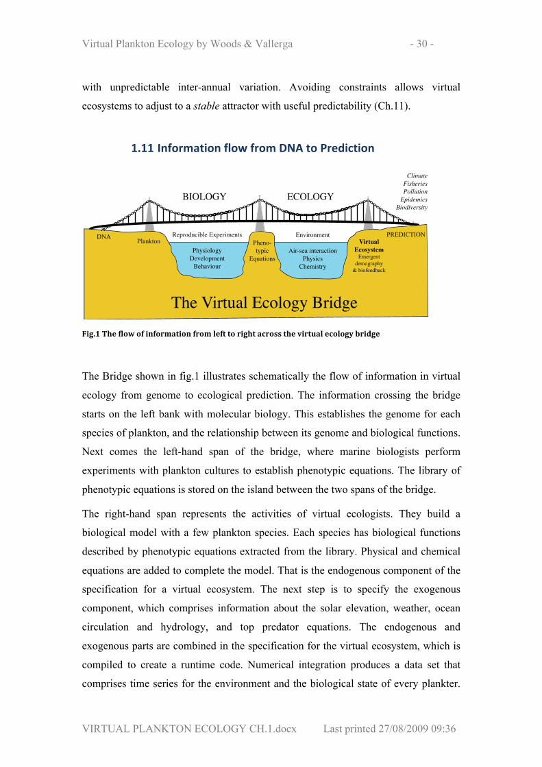
1.11 Information flow from DNA to Prediction

Fig.1 The flow of information from left to right across the virtual ecology bridge

The Bridge shown in fig.1 illustrates schematically the flow of information in virtual

ecology from genome to ecological prediction. The information crossing the bridge

starts on the left bank with molecular biology. This establishes the genome for each

species of plankton, and the relationship between its genome and biological functions.

Next comes the left-hand span of the bridge, where marine biologists perform

experiments with plankton cultures to establish phenotypic equations. The library of

phenotypic equations is stored on the island between the two spans of the bridge.

The right-hand span represents the activities of virtual ecologists. They build a

biological model with a few plankton species. Each species has biological functions

described by phenotypic equations extracted from the library. Physical and chemical

equations are added to complete the model. That is the endogenous component of the

specification for a virtual ecosystem. The next step is to specify the exogenous

component, which comprises information about the solar elevation, weather, ocean

circulation and hydrology, and top predator equations. The endogenous and

exogenous parts are combined in the specification for the virtual ecosystem, which is

compiled to create a runtime code. Numerical integration produces a data set that

comprises time series for the environment and the biological state of every plankter.

Reproducible Experiments

PhysiologyDevelopment

Behaviour

DNAPheno-typic

Equations

BIOLOGY ECOLOGY

VirtualEcosystem

Emergentdemography

& biofeedback

PREDICTION

ClimateFisheriesPollutionEpidemics

Biodiversity

The Virtual Ecology Bridge

PlanktonEnvironment

Air-sea interactionPhysics

Chemistry



The demography and biofeedback are diagnosed from those raw data. Together they

are the emergent properties of the simulation. Finally, on the right bank we see

predictions derived from these emergent properties. Some predictions help advance

the science of biological oceanography. Others serve applications in fisheries,

pollution, health and climate.

This schematic presentation emphasizes two important points made earlier. First, the

scientific integrity of virtual plankton ecology rests on the biological primitive

equations (phenotypic equations). And, second, the quintessential properties of the

ecosystem, demography and biofeedback, are emergent properties of virtual ecology.

These two properties are diagnosed from the primary emergent properties (values of

the state variables of the model). They are not in themselves state variables: the

specification for the virtual ecosystem contains no equations that have terms in

demography or biofeedback. So the virtual ecosystem develops freely without prior

assumption or constraint concerning those diagnostic properties. That is what

distinguishes virtual ecology from population ecology, in which the state variables are

demographic. We shall now comment further on that fundamental difference.

1.12 Comparison with population‐based modelling

The models of population ecology use demographic state variables. It is difficult to

understand the logic of that practice, which has dominated theoretical population

ecology since Lotka and Volterra (Murray 2003). Demography is a diagnostic

property of an ecosystem, and virtual ecology treats it as such. It lies on the right hand

side of the Bridge in fig.1. Population-based modelling uses inherently diagnostic

properties as state variables in prognostic equations.

Demography is an emergent diagnostic property of virtual ecosystems. We shall show

later that it is highly volatile (Ch. 20). Emergent properties respond significantly to

even quite small changes in the exogenous conditions that force the ecosystem. So

empirical relationships between them have limited validity. They refer to the attractor

of the virtual ecosystem when forced by a particular instance of exogenous forcing.

This led (Sutherland 1996) to comment, “Population ecology has usually been based

upon empirical relationships. This has the disadvantage that if the environment

changes it is necessary to re-determine those relationships.”



1.12.1 Prediction when the forcing changes The predictions of classical population ecology use population-based models that

contain empirical relationships (Sutherland 1996). The predictions rely on the method

of induction (Bacon 1620), which has been challenged by (Popper 1972). The method

fails when the exogenous conditions change making the ecosystem shift to a new

attractor, which has different relationships between emergent properties. It is not

logical to predict ecosystem response to climate change by models that depend on

empirical relations established in the past. Similar problems affect financial and

business modelling in time of rapid economic adjustment. For example, it is unwise to

use empirical relationships established in the past to plan a shipping business in

today’s changing global trade. The method of induction gives useful predictions only

in a stationary world. It’s strength lies in diagnosis, not in prognosis. Virtual ecology

does not depend on empirical relationships. It accurately tracks the change in attractor

as an ecosystem adjusts to changing forcing by exogenous factors including climate,

release of ballast water containing alien species, changing top predators by fishing,

accidental or purposeful fertilization of the ecosystem.

1.12.2 Bayesian comparison of LEM and PBM

Bayes’s theorem provides a way to assess the relative credibility of the two methods:

LEM and PBM. The comparison focuses on a well-observed ecological phenomenon

that each can simulate. The Bayesian approach assesses the credibility of each method

in terms of two probabilities: prior and posterior. The prior is generic: it depends on

the metamodel. The posterior is specific for a particular prediction: it depends on the

observational evidence exploited by the Ecological Turing Test, which requires

knowledge of the errors in the predictions (see §1.16 below). ETT alone satisfies the

statistical needs of Bayes’s method.

Table 1.12 compares significant features of the two methods that affect the prior and

posterior probabilities. Let us start by comparing the prior probability for each

method. Apart from the limited number of species, which is common to both

methods, the comparison of features all favour predictions by Lagrangian Ensemble

modelling over those by population-based modelling. In fact the list could have been

extended to include all the principles of virtual plankton ecology. We conclude that

we have a prior expectation that the LE metamodel is more likely to deliver



predictions that are useful for biological oceanography. In other words, it is more fit

for purpose.

Turning to posterior probability, we find that the PBM strange attractor gives large

errors to it’s predictions. That source of error is absent in the LEM. And the errors in

LEM predictions due to internal noise in the computation are much smaller. They are

estimated from the method of ensembles, which cannot be used in PBM. So it cannot

be used meaningfully in verification by the Ecological Turing test. In passing we note

that the ensemble method of estimating errors in predictions can be used in Monte

Carlo modelling, which is a version of PBM, but it is not commonly used in

biological oceanography.

To conclude, Bayesian assessment shows that LEM prediction is more likely to be

credible than PBM prediction of the same ecological phenomenon.

Table 1.12 Comparison of predictions by the LE and PB methods

Metamodel Lagrangian Ensemble Population-based

Prior probability Primitive equations

Intra-population variability

Exogenous closure

Stable attractor

Limited number of species

Diagnostic state variables

-

Endogenous closure

Strange attractor

Limited number of species

Posterior probability

Based on the

Ecological Turing test

Errors in predictions estimated from ensembles.

Errors in predictions estimated from inter-annual variability associated with the strange attractor. Note: Ensembles can be used to estimate errors in Monte Carlo modelling, but it is rare in biological oceanography.



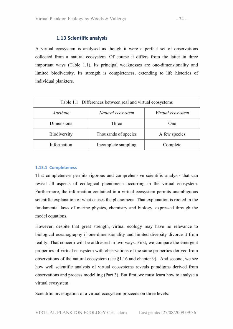
1.13 Scientific analysis

A virtual ecosystem is analysed as though it were a perfect set of observations

collected from a natural ecosystem. Of course it differs from the latter in three

important ways (Table 1.1). Its principal weaknesses are one-dimensionality and

limited biodiversity. Its strength is completeness, extending to life histories of

individual plankters.

Table 1.1 Differences between real and virtual ecosystems

Attribute Natural ecosystem Virtual ecosystem

Dimensions Three One

Biodiversity Thousands of species A few species

Information Incomplete sampling Complete

1.13.1 Completeness

That completeness permits rigorous and comprehensive scientific analysis that can

reveal all aspects of ecological phenomena occurring in the virtual ecosystem.

Furthermore, the information contained in a virtual ecosystem permits unambiguous

scientific explanation of what causes the phenomena. That explanation is rooted in the

fundamental laws of marine physics, chemistry and biology, expressed through the

model equations.

However, despite that great strength, virtual ecology may have no relevance to

biological oceanography if one-dimensionality and limited diversity divorce it from

reality. That concern will be addressed in two ways. First, we compare the emergent

properties of virtual ecosystem with observations of the same properties derived from

observations of the natural ecosystem (see §1.16 and chapter 9). And second, we see

how well scientific analysis of virtual ecosystems reveals paradigms derived from

observations and process modelling (Part 3). But first, we must learn how to analyse a

virtual ecosystem.

Scientific investigation of a virtual ecosystem proceeds on three levels:



1. Time series analysis, 2. Identification and documentation of ecological phenomena,

3. Scientific explanation of those time series and phenomena.

1.13.2 Time series analysis

Examples of time series analysis will be presented in chapter 10, which applies the

method illustrated in (Woods 2005) to a more complex plankton community.

Examples of emergent ecological phenomena are the spring bloom, or the transition

from seasonal to permanent oligotrophy. They are the included in the Twelve

paradigms of biological oceanography (Part 3; chapters 13-24).

1.13.3 Scientific explanation Here we consider the third level of analysis: scientific explanation. The goal is to

understand the temporal variations and ecological phenomena revealed in analysis at

levels 1 & 2. In general, scientific explanation involves relating observed phenomena

to the fundamental laws of nature. In virtual ecology that translates into relating

emergent phenomena revealed by level 1 & 2 analysis to the model equations that

were integrated to produce the virtual ecosystem. These equations have a special

status in virtual ecology. They are the primitive equations that represent the

fundamental laws of marine physics, chemistry and biology. The equations are

trustworthy because they were derived from reproducible experiments performed

under controlled experiments in the laboratory. They provide the scientific bedrock of

virtual ecology. The biological processes of individual plankters are described by

phenotypic equations. So scientific explanation stops digging at the properties of the

organism, its behaviour and physiology. Virtual ecology does not seek to explain

ecological phenomena in terms of biological processes inside the cell.

1.13.4 Audit trails A virtual ecosystem contains the life history of every biological particle in the virtual

mesoscosm, including living plankters, the corpses of dead plankters and planktogenic

detritus (fæcal pellets, etc.). Each life history is expressed as an audit trail comprising

time series of the biochemical state of the particle, and its ambient environment. The

audit trail is an emergent property of the virtual ecosystem that is directly controlled

by the phenotypic equations. Audit trails are the micro properties of the virtual



ecosystem. Scientific explanation involves establishing the causal link between an

emergent ecological phenomenon and audit trails.

1.13.5 Biofeedback The link comes from biofeedback, whereby each particle modifies its ambient

environment. Here are some examples. A phytoplankter affects the physical

environment by growing chlorophyll, which absorbs photons; that changes not only

the profile of solar irradiance but also the profile of turbulence. The phytoplankter

also changes the chemical environment by taking up nutrients. A zooplankter changes

the biological environment when it ingests prey, and changes the chemical

environment by excretion and egestion. Bacteria attached to a fæcal pellet

progressively release its chemicals into solution. Such influences on the physical,

chemical and biological environment can easily be computed from the audit trails of

individual plankters.

Summing the actions of individual plankters reveals the total biofeedback. That

allows us to explain the biological causes of macro changes in the environmental

fields. Ecological phenomena are usually expressed in terms of those fields.

Remember that the biological environment comprises fields of demographic variables

for each species featured in the virtual mesocosm. The demography of each species

includes the following emergent properties: its number density, the rate of increase

due to reproduction, and the rate of reduction due to each causes of death, including

starvation, being eaten, mortal disease, childbirth and old age.

1.13.6 Summary

To summarize, an ecological phenomenon is a bulk property. It is normally described

in terms of the evolving fields of physical, chemical and biological environment. The

plankton influence these fields by biofeedback. The magnitude of that biofeedback

can be computed by statistical analysis of audit trails, which record the life histories

of individual plankters. Each audit trail is controlled directly by the phenotypic

equations in the model used to create the virtual ecosystem. So analysis of audit trails

makes it possible to explain ecological phenomena in terms of the fundamental laws

of marine physics, chemistry and biology contained in the model equations.



In conclusion, it is worth noting that a virtual ecosystem is complete. It contains all

the information needed to explain ecological phenomena detected in it. There is no

need to invoke exogenous hypotheses. The explanation in terms of audit trails is

unambiguous (assuming the signal-to-noise ratio is fit for purpose, see §1.15).

Scientific analysis in terms of audit trails can always eliminate the mystery from an

unexpected phenomenon. Finally, we must remember that the scientific explanation

occurs within the context of the virtual ecosystem, which has far fewer species than

the natural ecosystem. Nevertheless, the completeness and lack of ambiguity of

virtual ecology are quite refreshing when compared with alternative methods

commonly used for scientific explanation in plankton ecology.

1.14 Prediction

Every virtual ecosystem is a prediction about how the environment and plankton will

change when the model equations are integrated under the constraints of the

exogenous conditions. We classify predictions in three ways: forecasting, hindcasting

and what-if? prediction.

1.14.1 Forecasting A forecast looks into the future. The pre-requisite is a method of forecasting future

development of the exogenous data used to force the simulation. For the atmospheric

boundary conditions that method is weather forecasting. In practice weather forecasts

are useful for about one week. That sets the limit of predictability in plankton

ecology.

1.14.2 Hindcasting Many ecological phenomena, including the twelve paradigms investigated in Part 3,

have intrinsic time scales that are much longer than the one-week limit of forecasting.

Investigating the annual growing season requires simulations lasting several years.

Chapter 6 simulates natural selection occurring over decades. And chapter 25 explores

the ecological response to climate change over one hundred years. To predict how the

ecosystem changes on these extended time scales we integrate the model with forcing

by exogenous data collected in the past. This procedure is called hindcasting. It

predicts how the virtual ecosystem would have developed during some specified



period in the past. This procedure was made possible by the recent compilation of “re-

analysis” data sets that describe the synoptic state of the atmosphere every six hours

during the last forty years (ERA40, see chapter 3). Integrating the model with

atmospheric forcing described by these “re-analysis” data creates a hindcast virtual

ecosystem.

1.14.3 What‐if? prediction

Operational oceanography supports planning of remedial actions to deal with marine

hazards such as pollution, toxic blooms and plankton-borne human diseases. Most of

the hazards have intrinsic time scales beyond the limits of predictability of weather

and therefore of the plankton ecosystem. So planning depends on hindcasts. The

strategy is to create virtual ecosystems that exhibit the hazard as an emergent

property. The nature of this hazard is likely to depend on (1) the details of the model

(including the model plankton community), and (2) on the exogenous forcing.

Sensitivity studies can map how the emergent hazard varies as these endogenous and

exogenous properties are altered. Having established the scope of the problem under

natural conditions, the next step is to see how it would change when remedial action is

taken. This involves introducing controlled events that modify the exogenous forcing.

The aim of What-if? prediction is to discover the effectiveness of candidate remedial

actions, and to establish which works best under different natural conditions. The

result is a plan that can guide the choice of action when the hazard occurs, taking

account of natural variations, such as the season and weather.

1.14.4 Initialization The success of prediction depends on first establishing a balanced virtual ecosystem.

Weather forecasting uses sophisticated mathematics for initialization (Lorenc 2002).

An early attempt at weather forecasting by (Richardson 1922) failed because it

omitted this crucial balancing step (Lynch 2006). It is equally important to achieve a

balanced state in a virtual ecosystem before attempting to diagnose ecological

processes occurring in it, or to make predictions. The feasibility of such balancing

was first demonstrated by (Woods, Perilli et al. 2005). They showed that a virtual

ecosystem spontaneously adjusts to a balanced state, a stable attractor, which is

independent of initial biological conditions.



During the transition from (exogenous) initial state to (emergent) attractor the

unbalanced components follow a damped oscillation. The oscillations of emergent

properties can have large amplitude, so it is essential that no conclusion be drawn

before they have decayed. The oscillations arise from interactions between biological

production in the plankton populations represented in the virtual ecosystem, and their

biofeedback to the environment.

Most biological production occurs in a brief growing season. It can be thought of as

an annual event. Adjustment to the attractor requires three or more such events.11 So

the balanced state is achieved only after the virtual ecosystem has existed for several

years. It is not possible to prevent the damped oscillation by basing initial conditions

on observations of just one component of the ecosystem such as mixed layer

chlorophyll estimated from ocean colour (Liu and Woods 2004). This important

subject will be considered further in chapters 11, 12 and 30.

1.15 Error analysis and control

Virtual ecology proceeds by a series of numerical experiments; each designed to

clarify some aspect of the plankton ecosystem, or to make a useful prediction. The

emergent properties, including environmental fields and life histories of plankters, are

the raw information of the simulation. Each synoptic value of an emergent property

has an associated uncertainty. Using the terminology of information theory, we call

the value “signal”, and the uncertainty “noise”. The quality of the emergent property

is measured by the signal-to-noise ratio. It is pointless to proceed with detailed

analysis of the virtual ecosystem if the raw emergent properties have a signal-to-noise

ratio of less than ten. The numerical experiments of virtual ecology are designed to

ensure that this criterion is achieved. This involves three tasks.

1. To identify the sources of error. 2. To measure the signal-to-noise ratio.

3. To control the error. Here we introduce them briefly. See Chapter 11 for more detail. We follow normal

practice in classifying errors as either systematic or random.

11 It is reminiscent of the three shots in naval gunnery: overshoot, undershoot, hit target.



1.15.1 Systematic errors

Systematic errors can arise in a virtual ecosystem from errors in the exogenous data

used to create the model or for forcing. They have an impact on the emergent

properties of the virtual ecosystem. The systematic error in a given emergent property

caused by the uncertainty in a particular source value can be assessed by classical

sensitivity analysis on a set of virtual ecosystems. Each simulation must last long

enough for the virtual ecosystem to adjust to the new attractor. We noted earlier that

virtual ecosystems are remarkably taut, so all emergent properties adjust to new

values when an exogenous source value is changed.

1.15.2 Random errors

Random errors in a virtual ecosystem arise from the Monte Carlo simulation of

plankter displacement by turbulence.

1.15.3 Measuring signal‐to‐noise

We use ensemble modelling to estimate the random errors in a virtual ecosystem. The

ensemble comprises a set of instances of the same virtual ecosystem. The model and

exogenous forcing are identical for each instance, with one exception. Each instance

is initialized with a different seed value for the random number generator. So a

different sequence of random numbers is used to compute successive turbulent

displacements of the plankton agent. In each instance the agent follows a different

trajectory, and therefore samples the environment differently and its plankters develop

differently. The set of trajectories in each instance produces a slightly different

demography for each population. Biofeedback creates a difference in the

environment. The result is that, while each instance in the ensemble is an equally

valid solution to the specified model and forcing, it settles on a slightly different

attractor. Statistical analysis reveals the ensemble mean values of the emergent

properties, and the inter-instance variability. The former is the signal; the latter is the

random noise due to turbulence. A worked example is presented in (Woods, Perilli et

al. 2005); see also chapter 11.

1.15.4 Controlling random errors

Using more computer agents to represent the plankton reduces the random errors in a

virtual ecosystem. It is good practice to ensure that the number of agents for each



biological state of a species does not fall below some prescribed number. This

criterion can be extended usefully to specifying a minimum number of agents in each

layer of the mesoscosm mesh. (Layers are typically one metre thick.) That is because

the rate of ingestion by a predator depends on the concentration of prey in the layer

where it resides. Experience suggests that the number of phytoplankton should be

represented by at least 200 agents per layer. A lower number leads to unacceptable

noise in all emergent properties.

The initial conditions are specified to exceed that minimum acceptable number of

agents per layer. However, as the integration proceeds, some agents have to be

removed from the computation because all the plankters in their sub-populations have

died or been eaten. In most virtual ecosystems there is a progressive decline in the

number of agents representing each species. The decline is faster in some layers. The

noise in the system rises as the number of agents (i.e. the number of independent

trajectories) declines. The rise in noise is countered by replacing the lost agents. That

is achieved automatically by adding new agents whenever the number falls below the

specified minimum. As each new agent is added it receives half the plankters of the

agent with the biggest sub-population. The plankton population remains unchanged

by this transfer, but the number of agents, and therefore the number of independent

trajectories is increased.

Splitting the largest sub-populations has the added benefit of narrowing the range of

sub-population sizes. That reduces the chance of a few exceptionally large sub-

populations biasing the estimate of demography.

1.16 Comparison with observations

Successful comparison with observations increases the credibility of a virtual

ecosystem. Here we consider how that comparison can be made. The starting point is

to recognize that there is uncertainty not only in an emergent property of a VE, but

also in an observation of the same property. We need to establish the noise in each

case before comparing the two signals.



1.16.1 Spatial resolution The comparison will be based on estimates of the average value of the chosen

property in a 1°x1° box. That area is determined by the spatial resolution of the

exogenous properties used to force the simulation (nutrients, weather, ocean

circulation, top predators, etc.). It is also the spatial resolution of the NOAA

climatology used to initialize the integration.

1.16.2 Temporal resolution

It is common practice to bin observations collected in the same month of the year

(NOAA), or to make time series of repeated observations at monthly intervals

(BATS). If they are collected during one year each monthly value may be treated as

synoptic. In that case the simulation must be computed using external forcing by the

actual weather in that year (e.g. from ERA40). On the other hand, the observations

may be climatic values calculated by averaging data collected in the same month of

the year over several years (e.g. NOAA Atlas). In that case the simulation can be

based on climatic forcing (e.g. from ERA40 and NOAA nutrient climate).

1.16.3 Strategy for comparison

Normally the comparison is based on existing observations, so the modeller must try

to create a virtual ecosystem that has the same space-time characteristics as the

observations. Perhaps in the future the order will be reversed, and experimental data

will be collected to test an existing prediction by a virtual ecosystem (see Ch.33).

Either way, it is likely that there will be a mismatch between the space-time

characteristics of observation and simulation. That will certainly be the case when

both are designed to represent the average conditions during one month (or less) in a

1°x1° box in the ocean. In that case the first task is to estimate the likely sampling

errors in two signals.

1.16.4 Choice of test variable We have noted earlier, that a virtual ecosystem is complete. It contains values of all

the state variables in the computation, plus derived properties such as demography.

Many of the state variables cannot be observed in nature: for example, the life

histories of individual plankters. That limits the choice of variable for comparison to



field properties. These include synoptic profiles of environmental properties such as

temperature, turbulence, chemical concentrations and demography.12

The list of observed properties is often quite limited. The modeller must extract

emergent properties that match the available observations. That may seem to limit the

value of the comparison. But it is not the case if the virtual ecosystem is in a balanced

state, i.e. on attractor. Then every property has a value that depends on the others.

Any change in forcing that directly perturbs one property soon leads to adjustment of

all the others, and the VE moves to a new attractor. This means we can choose to test

the virtual ecosystem by comparing any of its properties with observation. This is

why satellite ocean colour measurements of chlorophyll concentration in the surface

layer can be used to test the virtual ecosystem as a whole (Liu 2003; Liu and Woods

2004).

1.16.5 Comparing the timing of events

When the comparison is concerned with the timing of ecological events, the data

comprise time series of such properties sampled at the chosen location. That is an

eulerian time series based on samples of different bodies of water passing through the

site. It does not describe temporal changes in the same plankton community. The

water sampled on one day is likely to have drifted outside the 1°x1° box within a

month or so. In Ch.12 we shall see how the modeller can synthesize such an eulerian

time series from a large number of geographically-lagrangian simulations.

1.16.6 The Ecological Turing Test (Woods 2002) proposed a procedure for comparing observations with model

predictions. The aim is to see whether they could be representatives of the same

ecosystem. The approach echoes Turing’s well-known paper in which he looked into

the future when computing had become so sophisticated that one could not tell

whether one was addressing a person or a computer. That day has now arrived in call

centres that use computer-generated voices to answer customer queries. In our case

the quest is to discover whether the computer simulation could be describing the same

12 A virtual ecosystem is not discredited because it cannot predict a particular observed property; for example species that are not featured in the model plankton community. The aim of verification is to identify weaknesses that might be corrected.



ecosystem as the observations. The real benefit comes when it does not. If there is a

statistically significant gap between simulation and observations, then there must be

something wrong with the simulation. That gap becomes the spur for improvement.

How can one be sure that the difference between simulation and observation is

statistically significant? It depends on the uncertainty in each. The test succeeds if we

can be sure that despite the uncertainties, there is clear blue water between simulation

and observation. We need to quantify those uncertainties in the context of the space-

time conditions discussed above.

1.16.7 Uncertainty in the virtual ecosystem

The estimate of signal is based on the one-dimensional simulation; it does not take

account of patchiness caused by mesoscale turbulence. Furthermore, the model

plankton community has a tiny fraction of the species living in the 1°x1° box. The

shortcomings in modelling patchiness and species diversity are potential causes of

error. The VE contains no information about those errors; they are the unknown

uncertainty.

However we saw in §1.14 that we can use ensemble simulations to quantify the

internal errors due to using far fewer computer agents than the number of plankters in

the ecosystem. That is the known noise in the VE.

1.16.8 Uncertainty in the observation Assuming that the measurement errors are negligible, the uncertainty in an observed

property of the ecosystem lies in how well it represents the average value in the

1°x1°x1 month box. Ideally there would be sufficient observations in that box reliably

to estimate the mean value (the signal) and the standard deviation (the noise). That is

easier for variables that can be sampled continuously from a towed vehicle, such as a

batfish or Hardy-Longhurst continuous plankton recorder. However it is necessary to

bear in mind the fact that mesoscale turbulence produces a very patchy ecosystem. A

plankton net tow may sample a million litres of seawater, but that is only one part in

ten billion of the water in the top kilometre of the 1°x1° box. What is the chance that

the analysed concentrations of the top ten species of zooplankton deviate from the

actual mean values in the box by, say 50%?



1.16.9 A case study (Liu and Woods 2004) used the Ecological Turing Test (ETT) to compare the date of

the annual maximum concentration of chlorophyll in the mixed layer with SeaWifs

observations of ocean colour. They calculated the signal and noise from the mean and

standard deviation of a hundred SeaWifs pixels sampled in a 1°x1° box centred on

27°W 40°N. The intra-box variability was attributed to mesoscale patchiness. Ocean

colour was simulated by Monte Carlo optics with one billion photons in 64

wavebands. The photons were scattered/absorbed by the plankton profile simulated in

a virtual ecosystem. Ocean colour was computed from the photons that were scattered

up towards the satellite, using the action spectrum of the satellite radiometer. The

computation was repeated for each day of the year.

The test was to compare the dates of annual maximum surface chlorophyll

concentration. The result was a statistically significant difference. The virtual

ecosystem was then upgraded in two ways. First by switching from one population of

diatoms to an allometric set of three, which exhibited a seasonal succession (Nogueira

et al 2005).13 The second upgrade was to use a better algorithm for cloud radiation

interaction. The result of these two changes, one endogenous the other exogenous,

was to close the gap between observation and simulation. That exploited all the

information that SeaWifs had to offer for this test.

1.16.10 The value of comparing virtual ecosystems with observations

Historically modellers have used observations in two ways:

1. To tune model parameters.

2. To verify a model. Actually to find its deficiencies.

The first use is not applicable to virtual plankton ecology, which is based on primitive

equations. The values of parameters are determined from experiments. It is

inappropriate to change them to fit emergent properties to observations. Furthermore,

tuning is unwise in general, because it is valid only for a very limited set of 13 The three species were all diatoms, which contributed strongly to the mixed layer chlorophyll during the spring bloom off the Azores. Adding other species, such as dinoflagellates, which concentrate in the deep chlorophyll maximum, would have little impact on the comparison. The annual maximum of mixed layer chlorophyll is an example of a phenomenon that is relatively insensitive to species diversity. See the discussion at §1.2.4 above).



circumstances. And it squanders scarce observations that can better be used for

verification. It is much better to use observations to eliminate the shortcomings of the

model and the exogenous parametrizations used to force it. We have seen in the case

study above that verification and error correction quickly strips the value from

observations.

The specification of a virtual ecosystem leaves open many details that can be adjusted

without compromising the fundamental integrity that comes from using primitive

equations. The case study quoted above highlighted two adjustable features. The first

was the choice of species in the model plankton community. The second was the

algorithm used to compute the influence of clouds on insolation entering the ocean.

We saw that adjusting these, within a credible range, led to a better match between

predicted and observed dates of the annual maximum surface chlorophyll

concentration. That represents an effective use of observations to improve the virtual

ecosystem.

1.17 The Virtual Ecology Workbench

The computer programs used to create virtual ecosystems are complex. They are

difficult to write and to maintain. A typical investigation requires a sequence of

virtual ecosystems each having a slightly different specification. Each new version

needs to be tested and debugged before using. This can be time-consuming for such

complex programs. A full-time computer programmer is needed to support such

investigations. Or rather it used to be when the programming was done by hand. That

has now been replaced by a software tool, the Virtual Ecology Workbench (VEW),

which automates the programming and routine analysis of virtual ecosystems. The

user enters data and equations/rules through the graphical interface. When the

specification of a new virtual ecosystem is complete, the VEW automatically writes

executable code in Java, which can run on any personal computer that has a Java

compiler. (They almost all do.) Using the VEW reduces the turnaround time for

computing by a factor of one hundred, as compared with programming by hand. The

design and use of the VEW is described in Ch.7. The user handbook is included in the

DVD.



1.18 Summary

This chapter has opened discussion on two issues in modelling the plankton

ecosystem. The first concerns complexity, the second best practice.

1.18.1 Complexity

We started by comparing the computational complexity of a typical virtual ecosystem

with that of the natural ecosystem, focusing on three properties: environment,

demography, and biodiversity. This led to the following conclusions:

• The environment is very similar to the natural ecosystem, with one exception.

Current practice concentrates on one-dimensional simulations, which neglect

mesoscale turbulence. As the result the environment in a VE is much less complex

than in nature. Upgrading to three-dimensional virtual ecosystems will eliminate

this shortcoming. The complexity of the environment will then be comparable in

simulation and nature.

• Demography is computed from the life histories of individual plankters. The

virtual ecosystem uses agent-based modelling to simulate the plankton as

individuals. The limited power of computers restricts the number of agents to a

tiny fraction of the number of plankters. So the virtual ecosystem has many fewer

independent trajectories than the natural ecosystem. In that sense it is much less

complex. However, demography is computed from the statistics of the agents’

properties. The errors are acceptably low provided the simulation contains about

one million agents. That also applies to two other important ecological properties,

biofeedback and intra-population variability. For all these properties diagnosed

from agent data, the virtual and natural ecosystems have similar complexity.

• A virtual ecosystem has far fewer species than the natural ecosystem. There is no

way to eliminate this lack of complexity. So virtual ecosystems might provide a

misleading guide to the natural ecosystem. However many ecological phenomena

are insensitive to species diversity. Focusing on them, the strategy is to design

models that contain the species that most affect the phenomenon, and to

parametrize the others by functional groups. The magnitude of the error can be

assessed by sensitivity studies involving models that have different plankton

communities. The credibility of virtual plankton ecology ultimately rests on



demonstrating that it performs well in simulating ecological phenomena that have

been documented well by observations. The comparison uses the Ecological

Turing Test.

To summarize, virtual ecosystems are computationally complex, more so than

simulations created by population-based modelling, but less so than natural ecosystem

because they have many fewer species. Some ecological phenomena are insensitive to

that lack of species diversity.

1.18.2 Best modelling practice

The probability of success in simulating the plankton ecosystem is improved by

adopting best modelling practice. That was the second issue addressed in this chapter.

The subject is so big that it will occupy the next eleven chapters of this book. Chapter

1 briefly introduced fifteen topics, which we call the principles of virtual plankton

ecology. The aim was to show the scope of the subject before getting down to detail.

The starting point was primitive equation modelling, which has proved successful in

simulating other complex systems. The biological primitive equations are phenotypic:

they describe the functions of individual plankters. That led to individual based

modelling, and then to the Lagrangian Ensemble metamodel, which makes it possible

to compute demography and biofeedback as emergent properties. Mapping the

information flow from DNA to ecological prediction revealed the fundamental

difference between this practice and population-based modelling. The focus then

turned to downstream activities: scientific analysis and prediction, assessing and

controlling errors, and comparison with observations. The last topic introduced the

Virtual Ecology Workbench, which automates the main operations in virtual ecology,

thereby eliminating the need for computer programmers and experts in model

engineering for day-to-day research.

Taken together, these principles provide the scientific integrity that is essential for

creating trustworthy simulations of the plankton ecosystem. They ensure that

emergent properties have sound foundations in the laws of marine physics, chemistry

and biology; that the virtual ecosystem is on a stable attractor before we draw

conclusions from it; and that the signal-to-noise ratios of emergent properties are fit

for purpose.



1.18.3 Virtual Experiments

One last point: quite apart from its scientific value, virtual plankton ecology is great

fun. The Virtual Ecology Workbench takes away the chores associated with budgeting

and particle management, programming and data visualization. VEW Builder makes it

easy to create a new model with a selection of plankton species, plus functional

groups for those not represented. You can run the VEW on your laptop computer, but

the integration really flies if you use a quad-core desktop. Integration took less than

an hour per simulated year for the six-species virtual ecosystem in Chapter 10. The

VEW automatically documents each VE for future reference. This file is too large to

publish in the traditional way as an appendix to a scientific paper, but it can be made

available on the web. See examples on www.virtualecology.org. The documentation

of the Ch.10 VE is included in this book’s DVD.

One is likely to spend one hundred times longer exploring a virtual ecosystem than

creating it. So the VEW contains a powerful tool VEW Analyser to speed up selection

and plotting of emergent properties. When you load a new virtual ecosystem VEW

Analyser automatically configures the graphical user interface to display the time

series of its emergent properties tagged by geographical location, date and time. The

properties include environmental fields, demography and an audit trail for every

plankton agent. The graphical interface includes pull-down lists that make it easy to

select emergent properties with defined sampling in space and time. Analysing a

scientific phenomenon involves a sequence of data selections. At each step in that

analysis trail VEW Analyser automatically creates a file with the selected data, and

plots them as a time series, profile, space-time contour plot, or higher order products

such as a Poincaré map. The most fascinating aspect of scientific analysis comes from

audit trails, which show how individual plankters are contributing to the phenomenon.

(Yes, one starts to think in the present tense when exploring a virtual ecosystem.)

The images created on the screen by VEW Analyser provide vivid insights into how

the virtual ecosystem is working. One soon becomes immersed in its virtual world. It

seems very real. And if the virtual experiment (VEx) was carefully designed it

provides a realistic surrogate of nature. So what one discovers has a direct bearing on

scientific issues in biological oceanography. That is the joy of Virtual Experiments.



1.18.4 Conclusion We have chipped away at the objections commonly given for rejecting mathematical

simulation as a scientific contribution to biological oceanography.

1. The first step is to use best modelling practice. We have shown how that is

achieved by applying the principles of virtual plankton ecology. In passing we

noted that population-based modelling is less satisfactory for three reasons: it

neglects intra-population variability, and more importantly it uses intrinsically

diagnostic properties of the ecosystem as state variables in prognostic models,

furthermore it depends on empirical relationships that need to be revised if the

exogenous conditions change.

2. Today’s virtual ecosystems are one-dimensional and cannot therefore simulate

mesoscale turbulence, which causes patchiness in the plankton ecosystem.

Introducing three-dimensional virtual ecosystems will remove that objection.

3. The final objection is common to all methods of modelling the plankton

ecosystem. It is that the model plankton community has very few species

compared with the ocean. That objection is countered by demonstrating that

most ecological phenomena simulated in virtual ecosystems are not

particularly sensitive to such lack of species diversity. A modest increase in

the number of species is often sufficient to close the gap between prediction

and observation. The ecological phenomenon can then safely be analysed in

the virtual ecosystem. That produces improved understanding of the

phenomenon, which is the contribution virtual ecology makes to biological

oceanography.

The VEW provides the software technology to exploit this potential effectively.



References

Bacon, F. (1620). Novum Organum. Oxford, Clarendon Press. Baretta‐Bekker, J. G. and J. W. Baretta (1997). "European Regional Seas

Ecosystem Model (ERSEM II)." Journal of Sea Research.

Billari, F. C., T. Fent, et al., Eds. (2006). Agent‐based Computational Modelling: Applications in Demography, Social, Economic and Environmental Sciences Heidelberg, Physica‐Verlag Heidelberg.

Caswell, H. and M. G. Neubert (1998). "Chaos and closure terms in plankton food chain models." Journal of Plankton Research 20: 1837–1845.

DeAngelis, D. L. and L. J. Gross, Eds. (1992). Individual‐based models and approaches in ecology ‐ populations, communities and ecosystems. New York, Chapman & Hall.

Grimm, V. and S. G. Railsback (2005). Individual‐based Modeling and Ecology. Princeton, Princeton University press.

Kiørboe, T. (2008). A mechanistic approach to plankton ecology. Princeton, Princeton University Press.

Levitus, S. (1982). Climatological Atlas of the World Ocean, US Government Printing Office: 173.

Liu, C.‐C. (2003). Using seawifs ocean colour data to test a plankton ecosystem model, T.H. Huxley School for Environment, Earth Sciences and Engineering, Imperial College, London 2000.

Liu, C.‐C. and J. D. Woods (2004). "Prediction of ocean colour: Monte Carlo simulation in a virtual ecosystem based on the Lagrangian Ensemble method." International Journal of Remote Sensing 25: 921‐936.

Lomnicki, A. (1988). Population ecology of individuals. Princeton, Princeton University Press.

Lomnicki, A. (1992). Population ecology from an individual perspective. Individual‐based models and approaches in ecology. D. L. DeAngelis and L. J. Gross. New York, Chapman and Hall: 3‐17.

Longhurst, A. (1998). Ecological Geography of the Sea. San Diego, Academic Press.

Lorenc, A. C. (2002). Atmospheric data assimilation and quality control. Ocean forecasting. N. Pinardi and J. D. Woods. Berlin, Springer‐Verlag: 72‐96.

Lorenz, E. N. (1993). The essence of chaos. London, UCL Press.

Lynch, P. (2006). The emergence of Numerical Weather Prediction: Richardson's dream. Cambridge, Cambridge University Press.

Mangel, M. and C. W. Clark (1988). Dynamic modeling in behavioural ecology. Princeton, NJ, Princeton University Press.



May, R. M. (1977). Theoretical ecology: principles and applications. Oxford, Blackwell.

McGlade, J. M. (1999). Individual‐based models in ecology. Advanced ecological theory. J. M. McGlade. Oxford, Blackwell: 1‐22.

McGlade, J. M. and A. Novello‐Hogarth (1997). "Sustainable management of coastal resources: SimCoast a fuzzy logic rule based expert system." Hydro International 1: 6‐9.

Miller, C. B. (2004). Biological Oceanography. Oxford, Blackwell.

New, A. (2009). Developments in ocean, ice and ecosystem modelling at NOCS. Forecasting the state of our seas: the work of the National Centre for ocean forecasting. London, Royal Meteorological Society.

Pinker, S. (1997). How the mind works. London, Allen Lane. Popova, E. E., M. J. R. Fasham, et al. (1997). "Chaotic behaviour of an ocean

ecosystem model under seasonal external forcing." Journal of Plankton Research 19(10): 1495–1515.

Popper, K. (1972). Objective Knowledge: An Evolutionary Approach. Oxford, Oxford University Press.

Richardson, L. F. (1922). Weather prediction by numerical process. Cambridge, Cambridge Unicersity Press.

Scheffer, M., D. L. Baveco, et al. (1995). "A simple solution for modelling large populations on an individual basis." Ecological modelling 80: 161‐170.

Steele, J. H. and E. W. Henderson (1995). "Predation control of zooplankton demography." ICES Journal of Marine Science: 565‐573.

Sutherland, W. J. (1996). From individual behaviour to population ecology. Oxford, Oxford University Press.

Sverdrup, H. U. (1953). "On conditions for the vernal blooming of phytoplankton." Journal du Conseil international pour l"explration de la mer. 18: 287‐295.

Traub, J. F. and A. G. Werschulz (1998). Complexity and information. Cambridge, Cambridge University Press.

Waldrop, M. M. (1992). Complexity: the emerging science at the edge of order and chaos. New York, Simon and Schuster.

Woods, J. D. (2002). Primitive equation modelling of plankton ecosystems. Ocean Forecasting. N. Pinardi and J. D. Woods. Berlin, Springer‐Verlag: 377‐472.

Woods, J. D. (2005). "The Lagrangian Ensemble metamodel for simulating plankton ecosystems." Progress in Oceanography 7: 84‐159.

Woods, J. D. and R. Onken (1982). "Diurnal variation and primary production in the ocean – preliminary results of a Lagrangian ensemble model." Journal of Plankton Research 4: 735‐756.



Woods, J. D., A. Perilli, et al. (2005). "Stability and Predictability of a Virtual Plankton Ecosystem created with an individual‐based model." Progress in Oceanography 67: 43‐83.

Yager, R. R. and D. P. Filev (1994). Essentials of Fuzzy Modeling and Control. New York, John Wiley.

1. Principles of VPE

Documents