1 Particle Filtering for Multisensor Data Fusion with Switching Observation Models. Application to Land Vehicle Positioning Franc ¸ois Caron, Manuel Davy ? , Emmanuel Duflos and Philippe Vanheeghe INRIA-FUTURS ”SequeL” Laboratoire d’Automatique, G´ enie Informatique et Signal, UMR CNRS 8146 Ecole Centrale de Lille BP 48, Cit´ e Scientifique, 59651 Villeneuve d’Ascq Cedex [email protected], [email protected] [email protected], Philippe.Vanheeghe.fr Abstract This paper concerns the sequential estimation of a hidden state vector from noisy observations delivered by several sensors. Different from the standard framework, we assume here that the sensors may switch autonomously between different sensor states, that is, between different observation models. This includes sensor failure or sensor functioning conditions change. In our model, sensor states are represented by discrete latent variables, which prior probabilities are Markovian. We propose a family of efficient particle filters, for both synchronous and asynchronous sensor observations, as well as for important special cases. Moreover, we discuss connections with previous works. Finally, we study thoroughly a wheel land vehicle positioning problem where the GPS information may be unreliable because of multipath/masking effects. EDICS: SEN - FUS Index Terms Sequential Monte Carlo Methods, Particle Filter, Multisensor System, Data Fusion, Global Positioning System, Switching Observation Model, Fault Detection. I. I NTRODUCTION Statistical Bayesian filtering aims at computing the posterior probability density function (pdf) of a state vector x t ∈X from sequentially obtained sensor measurements, called observations. It relies, in the state-space formulation, on a state evolution model x t = f (x t-1 , v t ) (1) July 12, 2006 DRAFT

Welcome message from author
This document is posted to help you gain knowledge. Please leave a comment to let me know what you think about it! Share it to your friends and learn new things together.
Transcript

1
Particle Filtering for Multisensor Data Fusion
with Switching Observation Models.
Application to Land Vehicle PositioningFrancois Caron, Manuel Davy?, Emmanuel Duflos and Philippe Vanheeghe
INRIA-FUTURS ”SequeL”
Laboratoire d’Automatique, Genie Informatique et Signal, UMR CNRS 8146
Ecole Centrale de Lille
BP 48, Cite Scientifique, 59651 Villeneuve d’Ascq Cedex
[email protected], [email protected]
[email protected], Philippe.Vanheeghe.fr
Abstract
This paper concerns the sequential estimation of a hidden state vector from noisy observations delivered by
several sensors. Different from the standard framework, we assume here that the sensors may switch autonomously
between different sensor states, that is, between different observation models. This includes sensor failure or sensor
functioning conditions change. In our model, sensor states are represented by discrete latent variables, which prior
probabilities are Markovian. We propose a family of efficient particle filters, for both synchronous and asynchronous
sensor observations, as well as for important special cases. Moreover, we discuss connections with previous works.
Finally, we study thoroughly a wheel land vehicle positioning problem where the GPS information may be unreliable
because of multipath/masking effects.
EDICS: SEN - FUS
Index Terms
Sequential Monte Carlo Methods, Particle Filter, Multisensor System, Data Fusion, Global Positioning System,
Switching Observation Model, Fault Detection.
I. INTRODUCTION
Statistical Bayesian filtering aims at computing the posterior probability density function (pdf) of a state vector
xt ∈ X from sequentially obtained sensor measurements, called observations. It relies, in the state-space formulation,
on a state evolution model
xt = f(xt−1,vt) (1)
July 12, 2006 DRAFT

2
where f is a nonlinear function and vt is a white noise. In the following, the time index t is assumed to be an
integer, that is, t ∈ {1, 2, 3, . . .}. Eq. (1) can be equivalently written in terms of the conditional pdf xt ∼ p(xt|xt−1),
where ∼ means ’statistically distributed according to’. The state xt is assumed to evolve in a very general state
space X , which might be continuous and/or discrete1.
In complex problems, a single sensor is usually unable to provide full knowledge about the hidden state. It is then
necessary to achieve the fusion of several observations zk,t (k = 1, . . . , n) provided by n sensors. Each observation
is related to the hidden state by an observation probability law p(zk,t|xt).
Sensors delivering observations are generally assumed to be in their nominal state of work (i.e., a nominal
observation pdf pk,1(zk,t|xt) for each sensor k = 1, .., n). For example, the observation pdf of a camera may be
identified during a bright and non-smoggy day. However, in realistic contexts, the sensor functioning conditions may
change, resulting in an observation pdf that is quite different from the nominal one. This usually happen because
of, e.g., external environment changes or sensor damage. In such cases, it is necessary to detect that the sensor
is no more in its nominal state of work and, whenever possible, identify the true state of work of each sensor in
order to avoid dramatic state estimation errors. In our framework, this comes down to selecting an observation pdf
pk,j(zk,t|xt) in a list. In the camera example discussed above, the statistical relationship between the state xt and
an observation zk,t (k = 1, . . . , n) may undergo changes along the day, due to smog, dust or dawn. Other such
examples are provided in the Results Section below. The case of fatal sensor failure is also considered as a major
sub-case in the following.
A. Problem statement
In this paper, we address sequential estimation problems where a sensor may switch between states of work,
using Bayesian filtering. These states of work are denoted by discrete variables ck,t, where we adopt the convention
ck,t ∈ {0, . . . , dk} for k = 1, . . . , n. In the following, the ck,t’s are also referred to as latent variables, or sensor
states. Of course, the observation model is determined by ck,t. More precisely, for each sensor k = 1, . . . , n, there
are dk possible observation models, denoted (for sensor state ck,t ∈ {1, . . . , dk})
zk,t = hk,ck,t,t(xt) + wk,ck,t,t (2)
where hk,ck,t,t and wk,ck,t,t are the (nonlinear) observation function and observation noise of the observation model
ck,t of sensor k at time t. We adopt the following convention for the definition of the latent variables ck,t:
ck,t = 0 if the observation zk,t is independent of xt
ck,t = 1 if the sensor k is in its nominal state of work
ck,t = j, j ∈ {2, .., dk} if the sensor k is in
its jth state of work
1For the sake of clarity, we use a slight abuse of notation throughout the paper: though the state/observations may contain discrete components,
we denote the state probability distribution as a pdf with p(·|·).
July 12, 2006 DRAFT

3
When a sensor undergoes fatal failure, that is, when zk,t is statistically independent of xt, zk,t follows a vague pdf
denoted pk,0(zk,t). In the general case, the joint observation pdf for all the n sensors is written compactly as
zt ∼ p(zt|xt, ct) (3)
where
p(zt|xt, ct) =n∏
k=1
p(zk,t|xt, ck,t) (4)
and
p(zk,t|xt, ck,t) = δ0(ck,t)pk,0(zk,t) +dk∑
j=1
δj(ck,t)pk,j(zk,t|xt) (5)
with zt = {z1,t, . . . , zn,t} and ct = {c1,t, . . . , cn,t}. δa is the Dirac delta function centered on a.
The state transition equation (1) and the observation equation (3) being defined, the sequential Bayesian filtering
model is almost completely set. In order to make it complete, the prior probability that ck,t (for k = 1, . . . , n) is
in a given state j (j = 0, . . . , dk) is denoted αk,j,t. The αk,j,t’s represent the confidence we have in each sensor to
be in a given state, as
Pr(ck,t = j) = αk,j,t, 0 ≤ j ≤ dk (6)
where αk,j,t ≥ 0 and∑dk
j=0 αk,j,t = 1.
Let αt be the vector built from the individual αk,j,t’s for k = 1, . . . , n, and j = 0, . . . , dk. These confidence
variables are, in practice, quite difficult to tune a priori, because the sensors external conditions may change rapidly
and unexpectedly. In order to tune them adaptatively, we propose to define Markov evolution model for the vector
of probabilities αt, as follows
αt ∼ p(αt|αt−1) (7)
Of course, the pdf p(αt|αt−1) is defined so that the αk,j,t’s are probabilities for all t (i.e., they are positive and
sum up to one for each sensor k).
B. Estimation objectives and algorithms
Bayesian filtering aims at estimating the posterior pdf p(x0:t, c1:t, α0:t|z1:t) with a special interest in the marginal
posterior p(xt|z1:t). (The notation at1:t2 denotes all the elements of a vector a between times t1 and t2.) In general,
p(xt|z1:t) has a very complex shape, and cannot be calculated in closed-form. Sequential Monte Carlo methods
for Bayesian filtering [1], [2], [3], [4], [5] (also called particle filters) provide a numerical approximation of this
marginal pdf using a set of weighted random samples, called particles. More precisely, the particles x(i)0:t, with
weights w(i)t , approximate the posterior pdf p(x0:t|z1:t) thanks to the empirical distribution PN (dx0:t)
PN (dx0:t) 'N∑
i=1
w(i)t δex(i)
0:t(dx0:t) (8)
July 12, 2006 DRAFT

4
(for the sake of notational simplicity, we assume that the state reduces to xt, up to the end of this subsection).
This empirical distribution can be used to compute Bayesian estimates of the state vector x0:t. For example the
minimum mean squared error (MMSE) estimate is
Ep(x0:t|z1:t) [x0:t] =∫
X t+1x0:tp(x0:t|z1:t)dx0:t
≈∫
X t+1x0:tPN (dx0:t) =
N∑
i=1
w(i)t x(i)
0:t (9)
This approximation becomes more precise as the number N of particles increases [6]. Particle filters have many
good properties that make them attractive for practical problems.
• As opposed to Kalman filters-based algorithms (Extended [7] or Unscented [8] Kalman filters), they do not
assume Gaussian distribution. They can be implemented for arbitrary (multimodal or highly skewed) posterior
pdf, which arise in particular when faced with nonlinear observation and evolution models or non-Gaussian
noises [3]
• They can deal with hybrid state vector (both continuous and discrete), see e.g. [9]
• The tradeoff between estimation accuracy and computational load comes down to adjusting the number of
particles [3]
The standard particle filter algorithm is based on sequential importance sampling, with weight normalization. It
is presented in Algorithm 1 below.
Algorithm 1: Standard Particle filter
% Step 1.1 Initialization
• For particles i = 1, .., N , do
– Sample the initial state according to some initial distribution π0, that is x(i)0 ∼ π0(x0)
– Compute the initial weights w(i)0 = p(x
(i)0 )
π0(x(i)0 )
• Normalize the weights so that∑N
i=1 w(i)0 = 1
• For t = 1, 2, ... do
% Step 1.2 Iterations
– For particles i = 1, .., N do
∗ Sample the state at time t using the importance distribution q, that is x(i)t ∼ q(xt|x(i)
t−1, z1:t)
∗ Update the weight
w(i)t ∝w
(i)t−1
p(zt|x(i)t )p(x(i)
t |x(i)t−1)
qt(x(i)t |x(i)
t−1)
where the proportionality constant is such that∑N
i=1 w(i)t = 1
% Step 1.3 Resampling
– Compute
Neff =
[N∑
i=1
(w
(i)t
)2]−1
(10)
July 12, 2006 DRAFT

5
– If Neff ≤ η then resample the particles: duplicate particles with large weights and suppress particles with
low weights. The resulting particles are denoted x(i)t and their weights are w
(i)t = 1
N . (η is a threshold set
to, e.g., 0.8×N .)
– Otherwise, rename particles, that is, set x(i)t ← x(i)
t .
C. Main contributions and paper organization
This paper proposes several contributions. First, in Section II, we present the general framework, and the statistical
models chosen. Second, the switching sensor states model presented above is fully explored, and a family of
particle filtering algorithms especially designed for this model are presented, see Section III. In particular, we
propose efficient importance distributions for the state xt, the latent variables ct and the probabilities αt. Third, we
consider the important case where the sensors deliver their observations in an asynchronous way. Indeed, in practice,
there might be a different sampling device for each sensor, and these devices may not have the same sampling
frequencies, nor the same clocks, and the observations are collected at different times for different sensors. We also
discuss several important subcases:
• Binary valid/fail sensor states. In most applications, users have one observation model for each sensor,
corresponding to the nominal state of work. The important matter concerns possible sensor failures. In this
case, the state variable of sensor k is binary, i.e., ck,t ∈ {0, 1} for all t.
• A Rao-Blackwellized algorithm [3] is proposed, for cases where the state evolution and observation models are
linear and Gaussian. This enables easy sensor failure detection in already existing Kalman filter-based systems.
• Switching variance observation models are investigated, i.e. when the statistics of the additive noise wk,j,t
switch between different values, while the observation function hk,j,t = hk,t remains the same. These noise
characteristics changes may be caused by, e.g., external environment conditions which bring supplementary
noise.
In Section IV, we propose a survey of related approaches. In particular, the connections of our approach to Jump
systems with fixed priors, Jump Markov (Linear) Systems, and that of Hue et. al. [10] are discussed, as well as the
differences and relevance of our statistical jump model with respect to these models. Simulations concerning two
academic, synthetic data where sensors have two or three states of work, including sensor fatal failure are presented in
order to show the accuracy of the method. Comparisons are provided with Jump systems with fixed priors and Jump
Markov Systems. Various interpretations and possible extensions are also proposed. In Section V, a real example
is fully addressed. It concerns the localization of a land wheel vehicle where the sensors provide measurements
of steering, speed and GPS position, potentially corrupted due to multipath or mask effects. Several state-of-the-
art Bayesian estimation methods are tested, and our particle filtering approach, together with an unscented-based
approximation shows to have the best performance.
July 12, 2006 DRAFT

6
zt−1
αt−1
ct−1
xt−1
zt
αt
σt
ct
xt
σt−1
Observable
Non observable
Fig. 1. Overall Bayesian sequential model for multisensor fusion with switching observation models. The discrete vector ct indicates the
observation model of each sensor, with prior probabilities αt. The evolution of the hidden state xt and αt is tuned by the hyperparameter
vector σt which also evolves. The aim of this model is to estimate accurately the hidden state xt from the sensor measurements zt even though
the sensor state of work may be switching.
II. SEQUENTIAL BAYESIAN MODELS
In this section, we give details about the switching observation model. Moreover, we propose several explicit
evolution pdfs for the probabilities αt, and prior pdfs over the observations.
The parameters to be estimated are essentially the state vector xt and the discrete variables ct. We propose to
apply sequential Bayesian estimation of these parameters, based on the following evolution models
xt ∼ p(xt|xt−1, σt) (11)
ct ∼ Pr(ct|αt) (12)
αt ∼ p(αt|αt−1, σt) (13)
σt ∼ p(σt|σt−1) (14)
This general dynamic model is summarized in Fig. 1. It should be noted that, through the incorporation of the
Markov prior over αt, the sensor states ct are not i.i.d.. Actually, ct depends on the past values c0, . . . , ct−1 by
marginalizing out the α0, . . . , αt. These evolution models (also called prior pdfs) are:
• p(xt|xt−1,σt) is the state evolution model, defined in Eq. (1) for t = 1, 2, . . .. At time 0, it is assumed that
x0 ∼ p0(x0).
• Pr(ct|αt) is the prior over the sensor state variables ck,t, k = 1, . . . , n. It is defined as
Pr(ct|αt) =n∏
k=1
Pr(ck,t|αk,t) (15)
with
Pr(ck,t|αk,t) =dk∑
j=0
δj(ck,t)αk,j,t (16)
July 12, 2006 DRAFT

7
where αk,t = {αk,0,t...αk,dk,t}. The choice of probabilities αk,j,t is extremely sensitive for the correct
estimation of sensors state of work. Moreover, the αk,j,t’s might evolve, because sensor reliability decreases as
the sensor becomes older, for example. Consequently, these probabilities are considered as unknown parameters
with a Markov prior, and they are also estimated.
• The evolution model p(αt|αt−1) for αt is as a Dirichlet distribution for each sensor k = 1, . . . , n
(αk,0,t, . . . , αk,dk,t) ∼ D(σαk,tαk,0,t−1, . . . , σ
αk,tαk,dk,t−1) (17)
where σαk,t is a sensor specific coefficient which adjusts the spread of the αk,j,t’s. We recall the definition of
a Dirichlet distribution for a set of random variables (b0, .., bp) ∼ D(a0, .., ap)
D(a0, .., ap) =Γ(
∑pl=0 al)∏p
l=0 Γ(al)
p∏
l=0
bal−1l δ1(
p∑
l=1
bl) (18)
where Γ is the gamma function. In the important special case where ck,t ∈ {0, 1} (dk = 1), the Dirichlet
distribution reduces then to a beta distribution.
At time t = 0, we assume that αk,0 ∼ p0(αk,0). The coefficient σαk,t tunes the evolution of αk,t. In order
to avoid setting a fixed value for σαk,t (and thus fixed dynamics for αk,t) this coefficient is also estimated, as
explained below, Eq (19).
• p(σt|σt−1) is the hyperparameter transition equation. In many problems, it is assumed that the evolution
noise vt is Gaussian. In this case, each scalar component of vt is assumed to have variance (σvt )2. As these
variances have an important influence on the Bayesian filter behavior, it may be important to consider them
as unknowns. For each of these variances, the evolution model may be
log(σvt ) = log(σv
t−1) + λv (19)
where λv is a zero mean white Gaussian noise with fixed and known variance. The log function is used to ensure
that the variances remain positive. This can also be applied to the hyperparameter that tunes the evolution of αt,
denoted σαk,t above. A similar hyperparameter evolution model may be found in [9] where it is shown that letting
the hyperparameters follow this model robustifies the estimation. The shorthand σt = {σvt , σα
k,t|k = 1, .., n}denotes the full set of hyperparameters. In the following, the hyperparameter σv
t will be assumed as known
and fixed (considering that it is not the central point of this article) and the shorthand σt = {σαk,t|k = 1, .., n}.
The model defined above allows, in theory, the estimation of the augmented state composed of the state vector xt,
the discrete latent variables ct, the confidence coefficients αt and the hyperparameters σt. In the general case, it is
not possible to calculate the posterior p(x0:t, c1:t, α0:t,σ0:t|z1:t) in closed form at each time step. Particle filters [3]
are widely used and provide the most convincing approach to tackle such problems. In the following section, we
present several algorithms for synchronous/asynchronous sensor measurements, and for important special cases.
III. PARTICLE FILTERING ALGORITHMS FOR SWITCHING OBSERVATION MODELS
In this section, we present several particle filtering algorithms for switching observation models. The cases of
synchronous and asynchronous measurements are resp. addressed in Subsections III-A and III-B, where dedicated
July 12, 2006 DRAFT

8
algorithms are presented. In Subsection III-C, importance distributions are presented, some being designed for
the general switching observation model framework, and some especially for the special cases a) Binary case
valid/failing (ck,t ∈ {0, 1}), b) conditionally linear and Gaussian System and c) Switching observation variances.
A. SISR algorithm for synchronous sensors
In some cases, the measurements provided by the n sensors are synchronous, that is, all the sensors have the
same sampling frequency and the measurements from all the sensors arrive at the same time. The corresponding
algorithm is presented in Algorithm 2 below.
Algorithm 2: Particle filter for switching
observation models – Synchronous case
% Step 2.1 Initialization
• For particles i = 1, .., N sample2 x(i)0 ∼ p0(x0)
• For particles i = 1, .., N , sample σ(i)0 ∼ p0(σ0)
• For particles i = 1, .., N , sample α(i)0 ∼ p0(α0|σ(i)
0 )
• Set the initial weights w(i)0 ← 1
N
% Step 2.2 Iterations
• For t=1,2,... do
– For particles i = 1, .., N , do
∗ Sample the sensor state variable c(i)t ∼ q(ct|x(i)
t−1, α(i)t−1, zt)
∗ Sample the state vector x(i)t ∼ q(xt|x(i)
t−1, c(i)t , zt)
∗ Sample the probabilities α(i)t ∼ q(αt|α(i)
t−1, c(i)t , σ
(i)t−1)
∗ Sample the hyperparameter vector σ(i)t ∼ q(σt|σ(i)
t−1, α(i)t ,α
(i)t−1)
– For particles i = 1, .., N , update the weights
w(i)t ∝ w
(i)t−1
p(zt|x(i)t , c(i)
t )p(x(i)t |x(i)
t−1)
q(x(i)t |x(i)
t−1, c(i)t , zt)q(c
(i)t |x(i)
t−1, α(i)t−1, zt)
× p(c(i)t |α(i)
t )p(α(i)t |α(i)
t−1, σ(i)t )p(σ(i)
t |σ(i)t−1)
q(α(i)t |α(i)
t−1)q(σ(i)t |σ(i)
t−1, α(i)t ,α
(i)t−1)
(20)
– Normalize the weights so that∑N
i=1 w(i)t = 1
% Step 2.3 Resampling
– Compute Neff as in Eq. (10) and perform particle resampling whenever Neff < η , see Step 1.3 in
Algorithm 1.
The importance distributions q(·) used in Algorithm 2 are presented in Subsection III-C below.
2The pdfs p0(·) used in the initialization can be any pdf over the state space, e.g., uniform or derived from some heuristics.
July 12, 2006 DRAFT

9
B. SISR algorithm for asynchronous sensors
In many cases, the sensors are equipped with individual sampling devices which do not have the same sampling
frequencies nor the same clock. As a result, the measurements originating from each of the sensors are available
at different times. This requires a specific particle filtering algorithm, which is presented in Algorithm 3 below.
Algorithm 3: Particle filter for switching
observation models – Asynchronous case
% Step 3.1: Initialization
• This step is similar to Step 2.1 in Algorithm 2.
% Step 3.2: Iterations
• For t=1,2,... do
– Await the arrival of a new measure zk,t, delivered by sensor k, k = 1, . . . , n and, for particles i = 1, .., N ,
do
∗ Sample the state of sensor k as c(i)k,t ∼ q(ck,t|x(i)
t−1,α(i)k,t−1, zk,t)
∗ Sample the state variable x(i)t ∼ q(xt|x(i)
t−1, c(i)k,t, zk,t)
∗ Sample the sensor state probabilities α(i)k,t ∼ q(αk,t|α(i)
k,t−1, c(i)k,t, σ
(i)t−1) for sensor k
∗ Sample the relevant hyperparameters σα (i)k,t ∼ q(σα
k,t|σα (i)k,t−1, α
(i)k,t,α
(i)k,t−1)
– For particles i = 1, .., N , update the weights
w(i)t ∝ w
(i)t−1
p(zk,t|x(i)t , c
(i)k,t)p(x(i)
t |x(i)t−1)
q(x(i)t |x(i)
t−1, c(i)k,t, zk,t)
× p(c(i)k,t|α(i)
k,t)p(α(i)k,t|α(i)
k,t−1, σα (i)k,t )
q(c(i)k,t|x(i)
t−1,α(i)k,t−1, zk,t)q(α
(i)k,t|α(i)
k,t−1)
× p(c(i)k,t|α(i)
k,t)p(σα (i)k,t |σα (i)
k,t−1)
q(σα (i)k,t |σα (i)
k,t−1, α(i)t , α
(i)t−1)
(21)
Normalize the weights so that∑N
i=1 w(i)t = 1
% Step 3.3 Resampling
– This step is similar to Step 2.3 in Algorithm 2.
The principle of this algorithm is quite close to that of Algorithm 2. In the latter algorithm, however, the state
vector xt is updated each time a new observation arrives from one of the sensors. In practice, Algorithm 3 is more
likely to be used, as many new sensors incorporate a sampling/pre-processing unit.
The importance distributions used in Algorithm 3, as well as those of Algorithm 2, are described in the next
subsection.
July 12, 2006 DRAFT

10
C. Importance distributions
In Algorithms 2 and 3, particles are extended from time t−1 to time t using importance distributions denoted q(·).We have defined one for each of the variables, namely q(ct|x(i)
t−1,α(i)t−1, zt), q(xt|x(i)
t−1, c(i)t , zt), q(αt|α(i)
t−1, c(i)t ,σ
(i)t−1)
and q(σt|σ(i)t−1, α
(i)t , α
(i)t−1). Their choice is of paramount importance for particle filtering algorithm efficiency [2].
The selection of the state importance distribution q(xt|x(i)t−1, c
(i)t , zt) is not specific to our framework, i.e., it may be
one of the standard choices [2], [3]: the optimal importance distribution q(xt|x(i)t−1, c
(i)t , zt) = p(xt|x(i)
t−1, c(i)t , zt),
or approximations of it obtained by applying Extended/Unscented Kalman filtering [2], [11].
The choice of the importance distribution q(ct|x(i)t−1, α
(i)t−1, zt) is crucial and it is specific to our framework. A
first remark is that the number of possible values of vector ct isn∏
k=1
(1 + dk), and testing each possible combination
is not realistic. For optimal efficiency, it is necessary that the distribution q(ct|x(i)t−1,α
(i)t−1, zt) proposes the most
probable configurations, that is, the most probable states ck,t for each sensor, k = 1, . . . , n. Since the sensors are
likely to switch state independently of the other sensors, this importance distribution is written
q(ct|x(i)t−1, α
(i)t−1, zt) =
n∏
k=1
q(ck,t|x(i)t−1, α
(i)k,t−1, zk,t) (22)
where the individual importance distributions q(ck,t|x(i)t−1, α
(i)k,t−1, zk,t) are also used in Algorithm 3. The optimal
importance distribution is q(ck,t|x(i)t−1, α
(i)k,t−1, zk,t) = Pr(ck,t|x(i)
t−1,α(i)k,t−1, zk,t), defined by
Pr(ck,t|x(i)t−1, α
(i)k,t−1, zk,t) =
α(i)k,ck,t,t−1p(zk,t|ck,t,x
(i)t−1)∑dk
j=0 α(i)k,j,t−1p(zk,t|j,x(i)
t−1)(23)
As this optimal importance distribution cannot be computed analytically, we use an approximation of it as
importance function. Using an EKF step, the pdfs p(zk,t|j,x(i)t−1) for j = 0, . . . , dk are approximated by
p(zk,t|j,x(i)t−1) ' N (hk,j,t(x
(i)t|t−1), S
(i)k,j,t)
where x(i)t|t−1 = f(x(i)
t−1) is the state prediction and S(i)k,j,t is the approximated innovation covariance matrix defined
by
S(i)k,j,t = ∇h
(i)k,j,tQ
(i)t ∇h
(i)k,j,t
T + R(i)k,j,t
where R(i)k,j,t is the covariance matrix of the additive noise w(i)
k,j,t for sensor k and particle i (which reduces to
σ(i)k,j,t in case of scalar observations), Q
(i)t is the covariance matrix of the state evolution noise vt (which reduces
to its diagonal components {σv (i)t } in case of independent state components evolution) and
∇h(i)k,j,t =
∂hk,j,t(x)∂x
∣∣∣∣x=bx(i)
t|t−1
(24)
The importance distribution q(ck,t|x(i)t−1,α
(i)k,t−1, zk,t) is thus defined by
q(ck,t|x(i)t−1,α
(i)k,t−1, zk,t) =
α(i)k,ck,t,t−1N (hk,ck,t,t(x
(i)t|t−1), S
(i)k,ck,t,t
)∑dk
j=0 α(i)k,j,t−1N (hk,j,t(x
(i)t|t−1), S
(i)k,j,t)
(25)
The importance distributions q(αt|α(i)t−1, c
(i)t ,σ
(i)t−1) and q(σt|σ(i)
t−1, α(i)k,t,α
(i)k,t−1) can be chosen as the optimal
importance distributions, that is those that minimize the variance of the weights, conditional on the observations [3].
July 12, 2006 DRAFT

11
Actually, these can be computed in closed-form, and reject sampling [12] may be implemented whenever direct
sampling is not possible. Considering that the Dirichlet distribution is conjugate to the multinomial distribution, the
optimal importance distributions q(αk,t|α(i)k,t−1, c
(i)k,t, σ
α (i)k,t ) for each sensor are given by
q(αk,t|α(i)k,t−1, c
(i)k,t, σ
α (i)k,t ) = D(σ′ α (i)
k,t α′(i)k,t−1) (26)
where σ′ α (i)k,t = σ
α (i)k,t + 1 and α
′(i)k,j,t−1 =
σα (i)k,t
σα (i)k,t +1
α(i)k,j,t−1 + 1
σα (i)k,t +1
δc(i)k,t
(j) for j = 1, . . . , dk. For the full set
of sensors,
q(αt|α(i)t−1, c
(i)t ,σ
α (i)t ) =
n∏
k=1
q(αk,t|α(i)k,t−1, c
(i)k,t, σ
α (i)k,t ) (27)
Concerning the hyperparameter σαk,t−1, the optimal importance distribution is
q(log(σαk,t)|α(i)
k,t,α(i)k,t−1, σ
α (i)k,t−1) =
D(α(i)k,t; σ
αk,tα
(i)k,t−1)
D(α(i)k,t; σ
α (i)k,t−1α
(i)k,t−1)
×N (log(σαk,t); log(σα (i)
k,t−1), λα) (28)
D. Important special cases
In this subsection, we present additional details for three special cases, which have some importance in applica-
tions.
1) Binary valid/failing sensor states: The binary valid/failing sensor states case is of great importance. For
example, in the chemical industry, sensors are immersed into reagents which may be quite corrosive, making sensor
faults likely, and difficult to check on-site. Another example is that of autonomous vehicles, which need to check
the information from the sensors are valid in order to avoid dramatic state estimation errors which would result in
vehicle crash. For this case, we present the specific choices of the importance distributions q(ck,t|x(i)t−1, α
(i)k,t−1, zk,t)
and q(xt|x(i)t−1, c
(i)t , zt).
Here, the sensor states may be either j = 0 or j = 1. The importance distribution, q(ck,t|x(i)t−1, α
(i)k,t−1, zk,t)
reduces to
q(ck,t|x(i)t−1,α
(i)k,t−1, zk,t) ∝ (1− α
(i)k,1,t−1)p0(zk,t)δ0(ck,t)
+α(i)k,1,t−1N (hk,1(x
(i)t|t−1), S
(i)k,1,t)δ1(ck,t) (29)
Once c(i)k,t has been sampled in Algorithm 2 or in Algorithm 3, the state x(i)
t is sampled using q(xt|x(i)t−1, c
(i)t , zt),
which is a Gaussian distribution whose mean and covariance matrix are given by the multisensor extended Kalman
filter, as follows: First, compute the estimate
x(i)t|t = x(i)
t|t−1 +n∑
k=1
c(i)k,tK
(i)k,tν
(i)k,t (30)
where ν(i)k,t = zk,t − hk,1,t(x
(i)t|t−1) and the Kalman gain is
K(i)k,t = Σ(i)
t|t(∇h
(i)k,1,t
)T
R(i)k,1,t
−1 (31)
July 12, 2006 DRAFT

12
Finally, let
Σ(i)t|t =
[Σ−1
t|t−1 +n∑
k=1
c(i)k,t
(∇h
(i)k,1,t
)T
R−1k,1,t∇h
(i)k,1,t
]−1
(32)
and set q(xt|x(i)t−1, c
(i)t , zt) = N (xt; x
(i)t|t , Σ
(i)t|t). The advantage of this approach is that the extended Kalman filter
quantities are used to sample both c(i)k,t and x(i)
t , which saves computations. The other importance distributions are
as explained above.
2) Conditionally linear and Gaussian model: Another important special case is when the Bayesian model is
linear and Gaussian, conditional on the sensor state variable ct (and on the hyperparameters σt):
xt = Ftxt−1 + Gtvt (33)
zk,t = Hk,j,txt + wk,j,t (34)
with Ft the state matrix, Gt the noise transition matrix, vt a zero mean white Gaussian noise of covariance matrix
Qt, Hk,j,t the observation matrix for the sensor k in state j and wk,j,t the zero mean white Gaussian noise with
covariance matrix Rk,j,t. This case is important when we have an already existing Kalman filter working for a
given sensor state j, and we want to add the extra possibility of detecting sensor faults, or state of work switch. The
corresponding algorithm implements a bank of interacting Kalman filters, known as a Rao-Blackwellized particle
filter, or a Mixture Kalman Filter, see [13], [14], [15], [16], [17] for examples. The algorithm below concerns the
asynchronous case. The proposal distributions are those described in Subsection III-C.
Algorithm 4: Rao-Blackwellized particle filter for
switching observation models – Asynchronous case
% Step 4.1 Initialisation
• For particles i = 1, .., N sample x(i)0|0 ∼ p0(x0|0)
• For particles i = 1, .., N , sample Σ(i)0|0 ∼ p0(Σ0|0)
• For particles i = 1, .., N , sample σ(i)0 ∼ p0(σ0)
• For particles i = 1, .., N , sample α(i)0 ∼ p0(α0|σ(i)
0 )
• Set the initial weights w(i)0 ← 1
N
% Step 4.2 Iterations
• For t=1,2,... do
– Await the arrival of a new measure zk,t, delivered by sensor k, k = 1, . . . , n and, for particles i = 1, .., N ,
do
∗ Sample the sensor state variable c(i)k,t ∼ q(ck,t|x(i)
t−1|t−1, Σ(i)t−1|t−1, α
(i)k,t−1, zk,t)
∗ Sample the probabilities α(i)k,t ∼ q(αk,t|α(i)
k,t−1, c(i)k,t,σ
(i)t−1)
∗ Sample the hyperparameter vector σ(i)t ∼ q(σt|σ(i)
t−1, α(i)k,t, α
(i)k,t−1)
∗ Update mean and covariance matrix with a Kalman filter step (x(i)t|t ,Σ
(i)t|t) =KF(x(i)
t−1|t−1, Σ(i)t−1|t−1, c
(i)k,t, zk,t)
July 12, 2006 DRAFT

13
– For particles i = 1, .., N , update the weights
w(i)t ∝ w
(i)t−1
p(zk,t|c(i)1:t, z1:t−1)p(c(i)
k,t|α(i)k,t)
q(c(i)k,t|x(i)
t−1|t−1,Σ(i)t−1|t−1,α
(i)k,t−1, zk,t))
× p(α(i)k,t|α(i)
k,t−1)p(σ(i)t |σ(i)
t−1)
q(α(i)k,t|α(i)
k,t−1, c(i)k,t,σ
(i)t−1)q(σ
(i)t |σ(i)
t−1, α(i)t , α
(i)t−1)
(35)
– Normalize the weights so that∑N
i=1 w(i)t = 1
% Step 4.3 Resampling
– Compute Neff as in Eq. (10) and perform particle resampling whenever Neff < η , see Step 1.3 in
Algorithm 1.
3) Switching observation variances: A last important case is when the observation model hk, j, t in Eq. (2) of a
given sensor k does not change, but the additive white noise pdf may switch between pre-defined distributions [18].
The additive noise of the jth pdf is denoted wk,j,t. An interesting case is when all the wk,j,t, j = 1, . . . , dk are
zero-mean and monomodal, with different variances (we assume the noises are sorted so that wk,1,t has the smallest
variance whereas wk,dk,t the largest). Similar to the above cases, the importance distribution q(ct|x(i)t−1, α
(i)t−1, zt)
can be computed from the approximated optimal pdf using an EKF step.
An alternative solution consist of defining an evolution model for the variance of wk,t under the sensor state
j = 1. This simple solution, however, does not enable switching between discrete variance states, as there is a
continuity across the noise variances. An attractive solution consists of setting an upper bound on the variance of
wk,t and switching to the state j = 0 whenever the variance becomes too large, thus detecting sensor failure.
IV. DISCUSSION
In this section, we first survey previous related works, and we discuss their connection with our approach. Then,
we present an alternative interpretation and possible extensions. Some simulation results for synthetic data showing
the efficiency of the approach are proposed in Subsection IV-C (the real example of land vehicle positioning is
presented in the next section).
A. Previous works
Switching state-space models, or jump state-space models, have been widely studied in the literature. Such models
are composed of
• A discrete random indicator variable ct, with some statistical structure, which governs the behavior of the
statistical state-space model that switches from one model to another
• A state vector xt that evolves according to a stochastic evolution model p(xt|xt−1, ct)
• An observation vector zt that is related to the state vector xt through a stochastic observation model p(zt|xt, ct)
July 12, 2006 DRAFT

14
Different ways of defining the statistical structure of the indicator variable ct have been investigated3
• The ct’s may be defined as random iid variables with (known or unknown) fixed prior Pr(ct). In that case we
have
Pr(ct|c1:t−1) = Pr(ct)
• The ct’s may be defined as a discrete-time homogeneous Markov chain with (known or unknown) fixed
transition matrix, and then
Pr(ct|c1:t−1) = Pr(ct|ct−1)
These last models, known as Jump Markov Systems (JMS), have been widely studied in the literature, especially
when the state-space models are conditionnally linear and Gaussian (Jump Markov Linear Systems, JMLS) [19],
[20], [21]. Many algorithms have been defined to solve this estimation problem, mainly based on Gaussian mixture
approximations, like the Interacting Multiple Model (IMM) algorithm [22], [23], or the Generalized Pseudo-Bayes
(GPB) algorithms [24]. Efficient sequential Monte Carlo algorithms have then been defined for both JMS [9],
[25], [26] and JMLS [27], [15]. These algorithms have been successfully applied in various area like digital
communications [28], [29], multitarget tracking [30], [31], [32], fault diagnosis [13], [33], [34], geoscience [35] or
image processing [18].
In our model, we do not make such a Markovian assumption for the indicator variable ct, but for its prior αt.
By doing this, one has
Pr(ct|c1:t−1) =∫
Pr(ct|αt) Pr(αt|c1:t−1)dαt
and, through αt, ct is a priori dependent of the whole trajectory c1:t−1, which is more likely for the problem we
are considering. Our model thus introduces a memory over the past sensor states, rather than simply considering the
last one. This memory is tuned by the hyperparameters σαk,t (a high value results in a long memory and conversely).
This is of particular interest when considering sensor failures. For example, in chemical industry, the confidence in
a sensor will generally decrease with time. In land vehicle positioning, the confidence in the GPS should decrease
when GPS failures have occurred recently, because it indicates the vehicle is in an area where it is subjected to
multipath effects (an urban canyon for example). Our approach is compared to both iid and Markovian indicator
variable models in the Section IV-C where it is shown that our non stationary approach is more robust in case of
a change of statistical properties of the indicator variables.
Hue et. al. work [10] is the closest to our approach. They used a prior over the probabilities of the latent state
(the data association variable in [10], which is the counterpart of ct in this paper), and this prior could evolve.
However, its evolution model is defined implicitly, whereas we handle it explicitly with the reliability coefficients
αk,t. Moreover, in [10], a Gibbs sampler is used to update these quantities, whereas we have a computationally
cheaper, and efficient, importance distributions, see simulations below.
3As pointed out by a reviewer, a possible statistical structure could be an m-order Markov model where Pr(ct|c1:t−1) = Pr(ct|ct−m:t−1).
As we found no reference using such a model for jump systems, we didn’t provide a comparison of our approach with this potentially interesting
model.
July 12, 2006 DRAFT

15
B. Interpretations and possible extensions
An interesting interpretation of our model is that of mixture of pdfs. More precisely, for a sensor k, the
switching observation model with latent variable ck,t can also be interpreted as a single observation equation
denoted p(zk,t|xt,αk,t, σt) whose pdf is the mixture of the individual sensor state pdfs,
p(zk,t|xt, αk,t, σt) =dk∑
j=0
αk,j,tp(zk,t|xt, ck,t = j, σt) (36)
In this interpretation, the variable ck,t is the mixture latent variable, and the weights αk,j,t evolve with time,
as well as the individual pdf parameters xt and σt. A direct extension of our algorithm concerns unsupervised
sequential classification using time-varying mixtures of Gaussian.
C. Illustrating examples
In this subsection, we present simulations for two scenarios: The first one concerns a widely used academic
model with two sensors, one of which switches state. The second example concerns a conditionally linear and
Gaussian model where the two sensors may fail.
1) First example: Consider the following nonlinear model from [3], [36], [37]
xt+1 =12xt + 25
xt
1 + x2t
+ 8 cos(1, 2(t + 1)) + vt (37)
with vt ∼ N (0, 10) and x0 ∼ N (0, 10). We assume that two sensors deliver observations. Sensor #1 has two valid
and one faulty states of work, given by the following three observation models
z1,t =
xt + w1,0,t w1,0,t ∼ U([−25, 25]) if c1,t = 0x2
t
20 + w1,t w1,1,t ∼ N (0, 1) if c1,t = 1(xt−10)2
20 + w1,2,t w1,1,t ∼ N (0, 3) if c1,t = 2
(38)
where U([a, b]) is the uniform pdf on the interval [a, b]. The second sensor has only one nominal and one faulty
states of work corresponding to the following observation models
z2,t =
xt + w2,0,t w2,0,t ∼ U([−25, 25]) if c2,t = 0
xt + w2,1,t w2,1,t ∼ N (0, 2) if c2,t = 1(39)
Both sensor are assumed not totally reliable and thus may be faulty. Observations from sensors #1 and #2 are
synchronous. Algorithm 2 is applied over 100 time iterations with N = 500 particles. The importance distribution
for q(xt|x(i)t−1, c
(i)t , zt) is chosen to be based on an Extended Kalman Filter step. Sensor #1 follows the second
observation model in Eq. (38) for t ∈ T1 ∪ T2 with T1 = [10, 30] and T2 = [50, 70] and is faulty for t ∈ T4
where T4 = [70, 80]. For other time instants, Sensor #1 follows the first observation model in Eq. (38). Sensor
#2 is faulty for t ∈ T3 where T3 = [20, 50]. These faults are simulated by adding a random offset sampled from
U([−20, 20]) to the observations z1,t and z2,t.
In Fig.’s 2-6, we have reported the MAP/MMSE estimates at each time t of c1,t, c2,t, αt and the error et, where
et = xt −N∑
i=1
w(i)t x
(i)t (40)
July 12, 2006 DRAFT

16
The empirical standard deviation used to compute the 2-sigma bounds in Fig.’s 5 and 9 is computed by
σe =
√√√√ N∑
i=1
w(i)t
(x
(i)t −
N∑
i=1
w(i)t x
(i)t
)2
(41)
As can be seen, the sensor states are accurately estimated, and the mean squared error is kept low, thanks to the
ability to accurately switch from one observation model to another.
10 30 50 70 80 100
c=0
c=1
c=2
Time
Latent variable c1,t
of sensor 1
10 30 50 70 80 100
c=0
c=1
c=2
Time
Round Latent variable c1,t
of sensor 1
Fig. 2. (Top) Posterior probability of each state c1,t ∈ {0, 1, 2} at each iteration t = 1, . . . , 100. Black corresponds to a zero probability,
whereas white corresponds to probability one. (Bottom) MAP estimate of the sensor state c1,t ∈ {0, 1, 2} (white = estimated state). During
time intervals T1 = [10, 30] and T2 = [50, 80], the true state is c1,t = 2, during the time interval T4 = [70, 80] the true state is c1,t = 0,
and c1,t = 1 for any other time instants. The sensor states are accurately estimated.
20 50 100
c=0
c=1
Time
Latent variable c2,t
of sensor 2
20 50 100
c=0
c=1
Time
Round latent variable c2,t
of sensor 2
Fig. 3. (Top) Posterior probability of each state c2,t ∈ {0, 1} at each iteration t = 1, . . . , 100. Black corresponds to a zero probability,
whereas white corresponds to probability one. (Bottom) MAP estimate of the sensor state c2,t ∈ {0, 1} (white = estimated state). During the
time interval T3 = [20, 50], the sensor if faulty, and it is valid for any other time instant. The sensor state is correctly estimated.
July 12, 2006 DRAFT

17
10 30 50 70 80 1000
0.2
0.4
0.6
0.8
1
Time
Evolution of α1,1,t
and α1,2,t
Observation model n°1 of sensor 1Observation model n°2 of sensor 1Faulty model of sensor 1
20 50 1000
0.2
0.4
0.6
0.8
1
Time
Evolution of α2,1,t
Observation model of sensor 2Faulty observation model of sensor 2
Fig. 4. (Top) MMSE estimate of α1,0,t, α1,1,t and α1,2,t. During time intervals T1 = [10, 30] and T2 = [50, 80], the confidence in state 2
(that is α1,2,t) increases, while α1,1,t decreases. The opposite happens outside T1, T2 and T4. Both coefficients α1,1,t and α1,1,t decrease
during the interval T4. During the interval T3 = [20, 50], the α2,1,t decreases because the sensor is estimated to be faulty. It increases outside
of T3, because the sensor is estimated as valid. (Bottom) MMSE estimate of α2,0,t and α2,1,t. During the interval T3 = [20, 50], the α2,1,t
decreases because the sensor is estimated to be faulty. It increases outside of T3, because the sensor is estimated as valid.
0 20 40 60 80 100−30
−20
−10
0
10
20
30
Time
Error between estimate and true state2−sigma bound of the empirical distribution
Fig. 5. Evolution of the error et computed as in Eq. (40) (solid line). In dashed lines, the 2-sigma bounds are plotted. The 2-sigma bounds
increase and decrease, depending on the observation model used (some are less informative than others). In particular, when t ∈ T3 = [20, 50],
sensor 2 is estimated as faulty, and it does not provide information about the hidden state xt. Overall, the estimation accuracy is good, even
though the sensors models switch.
For this particular example, our approach has been compared to the approach when the prior probabilities of the
July 12, 2006 DRAFT
18
10 30 50 70 80 1000
0.5
1
1.5
Hyperparameter σ1,t
Time
σ 1,t
20 50 1000
2
4
6
Hyperparameter σ2,t
Time
σ 2,t
Fig. 6. (Top) Evolution of the hyperparameter σα1,t. This hyperparameter tunes the dynamics of the reliability coefficient α1,t. More precisely, the
value of σ1,t decreases at times t=30, 50, 70 80, to allow the reliability coefficients to quickly change. (Bottom) Evolution of the hyperparameter
σα2,t. This hyperparameter tunes the dynamics of the reliability coefficients α2,t.
ct are assumed fixed and known. These prior probabilities are set according to the relative frequencies of the states
on the interval [0, 100], thus α′1 =[
0.1 0.5 0.4]
and α′2 =[
0.3 0.7]
where
Pr(ck,t|ck,1:t−1) = Pr(ck,t) = α′k(ck,t + 1)
The importance function for the ck,t’s remain the same as for our approach, except that it priors are then time-
invariant and fixed to α′k. Results of this method for the same simulation are shown in Fig.’s 7-9. Similar simulations
has been performed 500 times. They showed that our method provides an absolute mean error that is 21% less than
the absolute mean error of the fixed prior approach.
2) Second example: Consider the following linear model [7], [14].
xt+1 =
1 T
0 1
xt +
12T 2
T
γt (42)
with γt ∼ N (0, 10) and T = 0.1 is the sampling period. Two synchronous sensors deliver observations, each of
them having one observation model only:
z1,t =[
1 0]xt + w1,t (43)
z2,t =[
0 1]xt + w2,t (44)
Both sensors are assumed potentially faulty. When the sensors are in their nominal state of work, it is assumed
that the noises have pdfs w1,t ∼ N (0, 2) and w2,t ∼ N (0, 1). Whenever these sensors become faulty, the variances
are assumed to follow the vague pdfs w1,t ∼ N (0, 100) and w2,t ∼ N (0, 100). This is a conditionally linear and
Gaussian model, which can be implemented with the Rao-Blackwellized algorithm similar to Algorithm 4, for the
synchronous case, however.
July 12, 2006 DRAFT
19
10 30 50 70 80 100
c=0
c=1
c=2
Time
Latent variable c1,t
of sensor 1
10 30 50 70 80 100
c=0
c=1
c=2
Time
Round Latent variable c1,t
of sensor 1
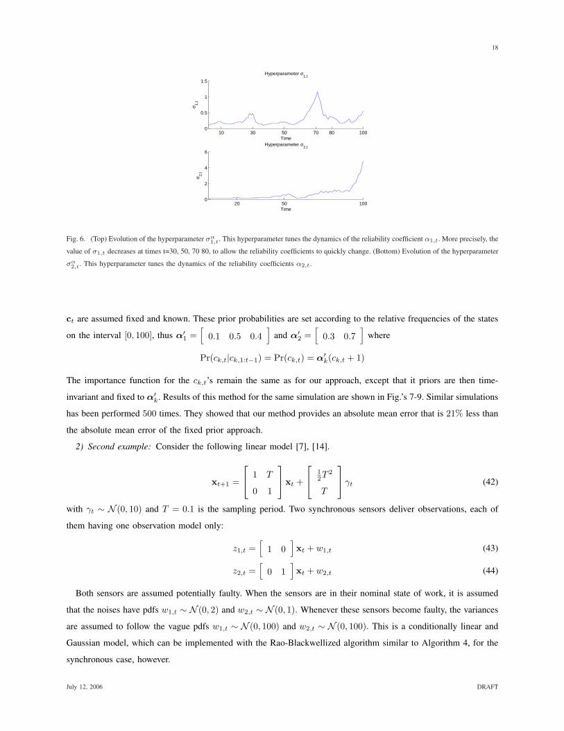
Fig. 7. (Top) Posterior probability of each state c1,t ∈ {0, 1, 2} at each iteration t = 1, . . . , 100 for the switching model with fixed priors. Black
corresponds to a zero probability, whereas white corresponds to probability one. (Bottom) MAP estimate of the sensor state c1,t ∈ {0, 1, 2}(white = estimated state). The sensor states are less accurately estimated, especially the sensor failure (c1,t = 0) during the time interval
T4 = [70, 80]
20 50 100
c=0
c=1
Time
Latent variable c2,t
of sensor 2
20 50 100
c=0
c=1
Time
Round latent variable c2,t
of sensor 2
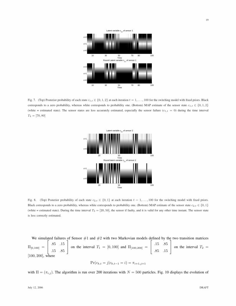
Fig. 8. (Top) Posterior probability of each state c2,t ∈ {0, 1} at each iteration t = 1, . . . , 100 for the switching model with fixed priors.
Black corresponds to a zero probability, whereas white corresponds to probability one. (Bottom) MAP estimate of the sensor state c2,t ∈ {0, 1}(white = estimated state). During the time interval T3 = [20, 50], the sensor if faulty, and it is valid for any other time instant. The sensor state
is less correctly estimated.
We simulated failures of Sensor #1 and #2 with two Markovian models defined by the two transition matrices
Π[0,100] =
.85 .15
.15 .85
on the interval T1 = [0, 100] and Π[100,200] =
.15 .85
.85 .15
on the interval T2 =
[100, 200], where
Pr(ck,t = j|ck,t−1 = i) = πi+1,j+1
with Π = (πi,j). The algorithm is run over 200 iterations with N = 500 particles. Fig. 10 displays the evolution of
July 12, 2006 DRAFT

20
0 20 40 60 80 100−30
−20
−10
0
10
20
30
Time
Error between estimate and true state2−sigma bound of the empirical distribution
Fig. 9. Evolution of the error et computed as in Eq. (40) (solid line) for the switching model with fixed priors. In dashed lines, the 2-sigma
bounds are plotted. The 2-sigma bounds increase and decrease, depending on the observation model used (some are less informative than others).
In particular, when t ∈ T3 = [20, 50], sensor 2 is estimated as faulty, and it does not provide information about the hidden state xt. The
absolute mean error is 20% higher than the error with our model.
the two components xt(1) and xt(2) of xt, as well as the observations z1(t) and z2(t). The MAP/MMSE estimates
of ct, αt and σt are displayed in Fig.’s 11–13, where the errors of position and velocity are defined by Eq. 40 for
each component of the vector xt.
As can be seen, the true sensor states are estimated very accurately, in spite of sensor failures. Simulations performed
with the same observations and a standard model (that is, the same model as in Eq.’s (42)–(44), without defining
a faulty sensor state) show a much higher error each time the sensors fail (for the sake of brevity this simulations
are not reported here ; see also the results in the following section).
Our model has been compared with a Jump Markov Linear System. The transition matrix of the JMLS is set to
Π = Π[0,100] =
.85 .15
.15 .85
. The algorithm employed is the optimal Rao-Blackwellised particle filter algorithm
provided by Doucet et al. [27]. Simulations have been run 500 times and the absolute mean position errors are
given in Tab. I for both models.
TABLE I
COMPARISON OF OUR MODEL WITH A JMLS
Model/Interval T1 T2 T1 ∪ T2
Abs. mean error of our model 0.6767 0.6241 0.6504
Abs. mean error of the JMLS 0.6149 0.7870 0.7070
Improvement −10.05% 20.70% 7.21%
The JMLS model provides better results on the first interval where the indicator variables are sampled according
to the fixed transition matrix Π, which was expected as the data are generated according to the evolution model.
July 12, 2006 DRAFT

21
0 50 100 150 200−60
−50
−40
−30
−20
−10
0
10Position
Time
Pos
ition
Estimated positionz
1 data
0 50 100 150 200−20
−15
−10
−5
0
5
10Velocity
Time
Vel
ocity
Estimated velocity
z2 data
Fig. 10. (Top) Evolution of the MMSE estimate of the first component xt(1) of xt as well as the observation z1(t) provided by sensor #1.
(Bottom) Evolution of the MMSE estimate of the first component xt(2) of xt as well as the observation z2(t) provided by sensor #2.
20 40 60 80 100 120 140 160 180 200
c=1
Time
True Latent variable c1,t
20 40 60 80 100 120 140 160 180 200
c=1
Time
MAP estimate of c1,t
20 40 60 80 100 120 140 160 180 2000
0.5
1
Reliability coefficient α1,t
Time
α 1,t
Fig. 11. (Top) True sensor state c1,t. Its evolution model follows the Markov transition matrix Π[0, 100] on the interval T1 = [0, 100] and
the Markov transition matrix Π[100, 200] on the interval T2 = [100, 200]. (Middle) MAP estimate of the the nominal sensor state c1,t = 1
(white = estimated state). (Bottom) MMSE estimate of the reliability coefficient α1,1,t. This coefficient decreases when the sensor is faulty.
However, on the second interval T2, our model outperforms the JMLS model, although it doesn’t define a Markov
structure on the indicator variables. As it is more realistic to consider that the dynamics of the indicator variables
may evolve with time, our algorithm provides a more robust estimation algorithm.
In the following section, we present an application of our framework to wheel land vehicle positioning.
July 12, 2006 DRAFT

22
20 40 60 80 100 120 140 160 180 200
c=1
Time
True latent variable c2,t
20 40 60 80 100 120 140 160 180 200
c_{2,t}=1
Time
MAP estimate of c2,t
20 40 60 80 100 120 140 160 180 2000
0.5
1
Reliability coefficient α2,t
Time
α 2,t
Fig. 12. (Top) True sensor state c2,t. Its evolution model follows the Markov transition matrix Π[0, 100] on the interval T1 = [0, 100] and
the Markov transition matrix Π[100, 200] on the interval T2 = [100, 200]. (Middle) MAP estimate of the the nominal sensor state c2,t = 1
(white = estimated state). (Bottom) MMSE estimate of the reliability coefficient α2,1,t. This coefficient decreases when the sensor is faulty.
20 40 60 80 100 120 140 160 180 200−4
−2
0
2
4
Time
Horizontal position error
Error between position estimate and true position2−sigma bound
20 40 60 80 100 120 140 160 180 200−4
−2
0
2
4
Time
Velocity error
Error between velocity estimate and true position2−sigma bound
Fig. 13. (Top) Evolution of the position error (solid line). In dashed lines, the 2-sigma bounds are plotted. The 2-sigma bounds increase and
decrease, depending on the observation model used (some are less informative than others). (Bottom) Evolution of the velocity error (solid line).
In dashed lines, the 2-sigma bounds are plotted. Overall, the estimation accuracy is good, even though the sensors models switch.
V. APPLICATION TO MULTISENSOR FUSION FOR LAND VEHICLE POSITIONING
The framework and algorithms presented above are well adapted to Mobile Robotics problems. Developing
autonomous vehicles such as drones or automated taxi cabs, is quite important for goods/people transportation
or operation in hostile environments (martian exploration, land mines removal). In order to ensure high accuracy
positioning and external environment mapping, many sensors, possibly redundant, are required. Typical positioning
sensors are GPS, inertial units, magnetic compasses. For obstacle detection, sensors may be radars or cameras.
An important characteristics of mobile robotics is that the observations delivered by some sensors may be easily
July 12, 2006 DRAFT

23
North
East
Speed encoder
a
North
H L
b
GPS sensor
P (X, Y )
β
ψ
Pc(Xc, Yc)
Fig. 14. Nomenclature of the vehicle. ψ is the angle between true North and longitudinal axis of the land vehicle and β is the steering angle.
Position is calculated at point P (X, Y ). Speed encoder is situated on the left rear wheel and GPS sensor on the front right side of the vehicle.
Position of the vehicle is calculated in the North-East coordinate frame.
blurred because of hard external conditions. For example, a camera lens may become dirty because of a sand
storm on Mars, and a radar may have additional noise due to snowfalls. Other sensors, like GPS are subject to
multipath phenomena in urban canyons and magnetic compass are sensitive to parasite electromagnetic fields: they
may deliver totally erroneous measurements in some conditions.
Several previous works apply sequential particle filtering to land vehicle positioning. Yang et al. [38] made
a comparative comparison between EKF and particle filter, showing the interest of the latter for the problem
considered. Giremus et al. [39] and Gustafsson et al. [16], [17] used a Rao-Blackwellized bootstrap filter. Giremus
et al. [40] proposed a fixed-lag Rao-Blackwellised particle filter to estimate multipath biases associated to the GPS
measurements. They used a switching observation model whose indicator variables have fixed priors.
In this section, we address the positioning of a land vehicle with four wheels, two of which may steer. The state
evolution model is presented in the next subsection.
A. State model based on land vehicle kinematics
The land vehicle considered is depicted in Fig. 14. Its kinematic model is inspired from [41] and [42]. The
differential equations governing the kinematics of the vehicle at point Pc are based on an Ackerman steering model
of simplified bicycle model (the variables are presented in Tab. II, here taken at point C):
Xc(t) = Vc(t) cos ψ(t)
Yc(t) = Vc(t) sin ψ(t)
ψ(t) = Vc(t)L tan β(t)
Let P (X, Y ) be the position of the vehicle at the GPS antenna (point P ). At point P , X and Y are expressed
July 12, 2006 DRAFT

24
TABLE II
STATE VARIABLES USED IN THE LAND WHEEL VEHICLE MODEL.
X , Y North and East positions of the vehicle at point P
V Speed of the vehicle at point PC
ψ Heading of the vehicle
β Steering angle
T Sampling time
as functions of Xc and Yc byX(t) = Xc(t) + a cos ψ(t) + b sinψ(t)
Y (t) = Yc(t) + a sin ψ(t)− b cosψ(t)
We adopt the following discrete first order approximation (where we note Vt = Vc(t))
Xt+1 = Xt + T
[Vt cosψt + (−a sin ψt + b cos ψt)
Vt
Ltan βt
]
Yt+1 = Yt + T
[Vt sinψt + (a cos ψt + b sin ψt)
Vt
Ltan βt
]
Vt+1 = Vt + T Vt
ψt+1 = ψt + TVt
Ltan(βt)
βt+1 = βt + T βt
βt+1 = βt + T βt
These equations may be rewritten as the following nonlinear model
xt+1 = f1(xt) + Gt · vt (45)
where f1 is the state transition function, Gt is the noise transfer matrix, the state vector is
xt = [Xt, Yt, Vt, ψt, βt, βt, ]T and vt = [Vt, βt]T . The state noise vt = [Vt, βt]T is assumed zero mean
white Gaussian with known covariance matrix Qt = E[vtvTt ].
B. Observation models
The vehicle is equipped with three sensors, see Fig. 14. These sensors are:
• A centimeter-level precision DGPS receiver, providing North and East position of the vehicle
• A speed sensor
• A steering sensor
Speed and steering measurements are synchronous. However, the GPS measurements are asynchronous w.r.t.
these other two sensors. The GPS measurements frequency is low (5 Hz) when compared to the Speed/Steering
measurement frequency (40 Hz). We detail below the sensor observation equations.
July 12, 2006 DRAFT

25
1) GPS sensor model: The observation model for the GPS is given by
z1,t = h1(xt) + w1,t =
Xt
Yt
+ w1,t
with w1,t a zero mean white Gaussian noise of known covariance matrix R1,t =
0.002 0
0 0.002
. When the
sensor is non-faulty, the likelihood is written as p(z1,t|xt) = N (h1(xt), R1,t).
The GPS receiver cannot be assumed fully reliable due to multipath, diffraction and mask phenomena likely to
alter the measurements, especially in urban areas [43]. It is supposed that the GPS sensor has two classes of work:
• A nominal state of work corresponding to the measurement model defined above
• A faulty state of work when data are corrupted by multipath. In that case we define a vague pdf p0(z1,t),
uniform on a large interval centered about the last position estimate
This is thus a sensor for which the discrete variable c1,t is in {0, 1} (binary case). The evolution pdf for α1,t is
that of Eq. (17).
2) Speed and Steering sensors: The observation models of the speed and steering sensors are respectively
z2,t = h2(xt) + w2,t = (1 + tan(βt)H
L)vt + w2,t
and
z3,t = h3(xt) + w3,t = βt + w3,t
with w2,t and w3,t zero mean white Gaussian noises of assumed known covariances matrix R2,t = 0.1 and
R3,t = 0.002. These sensors are not supposed to be faulty.
C. Estimation objectives and algorithm
Given the model and assumptions about the sensors, the estimation objective is as follows: each time the
speed/steering measurements are collected, we estimate xt by MMSE. Whenever a GPS measurement is collected,
we estimate xt, α1,t and σα1,t by MMSE and c1,t by MAP.
In this model, components of the state evolution noise have a negligible variance (almost deterministic evolution).
This makes the design of an efficient importance distribution q(xt|x(i)t−1, c
(i)t , zt) quite difficult: on the one hand,
using the state evolution pdf p(xt|x(i)t−1) as q(xt|x(i)
t−1, c(i)t , zt) (bootstrap filter choice) is not efficient. On the other
hand, UKF and EKF based approaches cannot be applied because the evolution model is highly informative and
the particle states x(i)t sampled from such importance pdfs are very likely to have very small weights.
Here, however, the posterior distribution p(xt, ct, αt, σt|z1:t) is almost always monomodal and little skewed.
We propose to use an approximate particle filtering approach, whose computational load is reduced, and which
is very accurate. This approach, proposed in [44] under the name of Rao-Blackwellised UKF, is inspired by the
Rao-Blackwellized particle filter, where the Kalman filters are replaced by Unscented Kalman filters [8], [45], [46],
[11]. Here, the state xt is estimated by a bank of UKFs, whereas the other parts of the full state (that is, ct, αt, σt)
July 12, 2006 DRAFT

26
are updated using the importance distributions described in Section III, for variables c1:t, α0:t, σ0:t are as explained
in Section III. The algorithm is presented below.
Algorithm 5: Rao-Blackwellized UKF particle filter
for switching observation models – Asynchronous case
% Step 5.1 Initialisation
• For particles i = 1, .., N sample x(i)0|0 ∼ p0(x0|0)
• For particles i = 1, .., N , sample Σ(i)0|0 ∼ p0(Σ0|0)
• For particles i = 1, .., N , sample σα (i)1,0 ∼ p0(σα
1,0)
• For particles i = 1, .., N , sample α(i)1,0 ∼ p0(α1,0|σ(i)
1,0)
• Set the initial weights w(i)0 ← 1
N
% Step 5.2 Iterations
• For t=1,2,... do
– Await the arrival of new measure zk,t, delivered by sensor #k, k = 1, 2, 3 and, for particles i = 1, .., N ,
do
% If arrival of measures z2,t and z3,t
∗ Update mean x(i)t|t and covariance matrix Σ(i)
t|t with a Unscented Kalman filter step, that
is (x(i)t|t , Σ
(i)t|t) = UKF(x(i)
t−1|t−1, Σ(i)t−1|t−1, z2,t, z3,t)
∗ update of variables related to the GPS sensor
∗ set c(i)1,t ← c
(i)1,t−1
∗ set α(i)1,t ← α
(i)1,t−1
∗ set σα (i)1,t ← σ
α (i)1,t−1
– For particles i = 1, .., N , update the weights
w(i)t = w
(i)t−1p(z2,t|z1:t−1)p(z3,t|z1:t−1)
% If arrival of a GPS measure z1,t
∗ Sample the sensor state variable c(i)1,t ∼ q(c1,t|x(i)
t−1|t−1,Σ(i)t−1|t−1, α
(i)1,t−1, z1,t)
∗ Sample the probabilities α(i)1,t ∼ q(α1,t|α(i)
1,t−1, c(i)1,t, σ
α (i)1,t−1)
∗ Sample the hyperparameter vector σα (i)1,t ∼ q(σα
1,t|σα (i)1,t−1, α
(i)1,t, α
(i)1,t−1)
∗ Update mean x(i)t|t and covariance matrix Σ(i)
t|t with a Unscented Kalman filter step, that
is (x(i)t|t , Σ
(i)t|t) =UKF(x(i)
t−1|t−1,Σ(i)t−1|t−1, c
(i)1,t, z1,t)
– For particles i = 1, .., N , update the weights
w(i)t ∝ w
(i)t−1
p(z1,t|c(i)1,1:t, z1:t−1)p(c(i)
1,t|α(i)1,t)
q(c(i)1,t|x(i)
t−1|t−1, Σ(i)t−1|t−1, α
(i)1,t−1, z1,t)
× p(α(i)1,t|α(i)
1,t−1, σα (i)1,t )p(σα (i)
1,t |σα (i)1,t−1)
q(α(i)1,t|α(i)
1,t−1, c(i)1,t, σ
α (i)1,t−1)q(σ
α (i)1,t |σα (i)
1,t−1, α(i)1,t,α
(i)1,t−1)
(46)
July 12, 2006 DRAFT

27
– Normalize the weights so that∑N
i=1 w(i)t = 1
% Step 5.3 Resampling
– Compute Neff as in Eq. (10) and perform particle resampling whenever Neff < η , see Step 1.3 in
Algorithm 1.
D. Results
Algorithm 5 is applied to real sensor measurements. These observations have been collected by the Australian
Center for Field Robotics (ACFR)4. These very clean data were not altered by the standard observations errors.
Two types of errors have been added to GPS signal to test the algorithm:
• Simulation of multipath and diffraction, by addition of a piecewise constant random offset to the real, non
altered data, see Fig. 15. Multipath are simulated at times in T1 = [50, 60], T2 = [62, 68] and T3 = [75, 80]
(time instants corresponds to GPS data indexes, i.e., it is increased by t ← t + 1 each time a GPS observation
is collected).
• Simulation of side-slipping of the vehicle, simulated by replacing the real steering angle observations by
erroneous ones, over the interval T4 = [12, 14] (see Fig. 16).
−4 −2 0 2 4 6 8−25
−20
−15
−10
−5
0
5Trajectory of the land vehicle
Y East (m)
X N
orth
(m
)
UKF+PF estimated positionGPS data
Multipath
Fig. 15. MMSE Estimation of the trajectory of the vehicle obtained using our algorithm. Squares represent the GPS data. Both are plotted in
the North-East coordinate frame. GPS failures occur due to multipath effects, these have been simulated by adding a piecewise constant random
bias to the true GPS observation.
The state estimation results of Algorithm 5 have been compared to those obtained by two Unscented Kalman
filters. In the first UKF, the ability to detect sensor failures is not implemented. In the second UKF, sensor failures
are detected from the normalized quadratic innovation, as detailed in Appendix A.
4These data may be found at the Internet address http://www.acfr.usyd.edu.au/homepages/academic/enebot/dataset.
htm.
July 12, 2006 DRAFT

28
4.5 4.6 4.7 4.8 4.9 5−2.5
−2
−1.5
−1
−0.5
0
0.5
Zoom on the side−slip
Y East (m)
X N
orth
(m
)
UKF+PF estimated positionUKF(with rejection) estimated positionGPS data
Fig. 16. MMSE Estimation of the trajectory of the vehicle, obtained with our algorithm and with a UKF algorithm which rejects invalid
measures. The segment of the trajectory represented here is a magnified view of Fig. 15. Vehicle side-slip is simulated by adding a random
offset to the steering measurement angle. In this case, the UKF algorithm rejects GPS data and fails in tracking again the true vehicle trajectory.
Our algorithm first rejects GPS data, but comes back to the true trajectory.
Fig. 17 represents the evolution of the posterior probability of c1,t for the GPS sensor. It also shows the MMSE
estimate of α1,t (which is here interpreted as a reliability coefficient). During intervals T1, T2 and T3, our algorithm
succeeds at detecting GPS failure and c1,t is estimated close to 0. The parameter α1,t drops during these intervals
from 80% to 40% GPS reliability.
Fig. 18 compares the positioning of our algorithm and that of the first UKF (which does not enable GPS
failure detection). Of course, this UKF performs poorly whenever erroneous measurements arrive, because they are
integrated in the fusion process, resulting in large errors during time intervals T1, T2 and T3. Our algorithm, on
the other hand, keeps good performance, though the error increases slightly over T1, T2 and T3. The error increase
is due to the lack of GPS information, and not to the algorithm itself.
Fig. 19 is similar to Fig. 18. In Fig. 19, however, our algorithm is compared to the UKF with erroneous
observations detection, see Appendix A. The latter algorithm considers the GPS measurements as erroneous (steering
measurements are assumed reliable), however, it fails at coming back to the true trajectory. This can be explained
as follows: due to side-slip, GPS measurements disagree with the evolution model during time interval T4 and they
are rejected by the UKF algorithm. As a consequence, the estimated vehicle trajectory diverges from the true one
as time increases, involving rejection of all the following GPS measurements: the UKF algorithm assumes wrongly
that the GPS is failing. The same phenomenon happens in case of GPS errors due to multipath problems in time
intervals T1, T2 and T3 (see Fig. 19). On the contrary, our algorithm tests all the sensor valid/failure hypotheses.
For example, at time t = 12, the most likely hypothesis is ”the GPS is faulty”, but at t = 13, the most likely
hypothesis becomes ”the GPS is valid” because the new GPS observation is coherent with the evolution model.
This explains that the position estimated by our algorithm follows the true trajectory (see Fig. 16).
July 12, 2006 DRAFT

29
20 40 50 60 68 75 80 100
c=0
c=1
Time
GPS latent variable c1,t
20 40 50 60 68 75 80 1000
0.5
1
GPS Time index
α 1,t
GPS reliability coefficient α1,t
Fig. 17. (Top) Posterior probability of the GPS state c1,t = 1. During time intervals T1 = [50, 60], T2 = [62, 68] and T3 = [75, 80], the
true state of GPS sensor is c1,t = 0 (faulty), and c1,t = 1 for any other time instants. The sensor states are accurately estimated. (Bottom)
MMSE estimate of the GPS reliability coefficient α1,1,t. During the intervals T1 = [50, 60], T2 = [62, 68] and T3 = [75, 80], GPS reliability
coefficient α1,1,t decreases because the GPS is detected to be faulty. Outside of these intervals, GPS reliability coefficient increases because
GPS is detected to be valid.
20 40 50 60 68 75 80 1000
0.2
0.4
0.6
0.8
1
1.2
1.4
GPS time index
Hor
izon
tal p
ositi
on e
rror
(m
)
Horizontal position error
UKF+PFUKF(without rejection)
Fig. 18. Comparison of the mean square positioning error between our algorithm and UKF algorithm (without detection of sensor failures).
UKF algorithm gives large errors during time intervals T1 = [50, 60], T2 = [62, 68] and T3 = [75, 80] (GPS failures) because it uses these
data into the fusion algorithm, as if they were reliable. Our algorithm largely outperforms UKF algorithm.
VI. CONCLUSION AND PERSPECTIVES
In this paper, we have proposed new model and algorithm for sensor failure detection and, more generally,
to switching observation models. We propose a family of algorithms for situations where the sensors deliver
measurements in a synchronous way, or in an asynchronous way. We proposed an alternative interpretation of our
model in terms of mixture of pdfs. Simulation results for two academic problems, and for a real wheel land vehicle
positioning problem show the interest of our model, and the efficiency of the proposed particle filter algorithms.
Extensions of this work will concern sequential unsupervised data classification. Further applications are in chemical
processes monitoring and visual tracking.
July 12, 2006 DRAFT

30
20 40 50 60 68 75 80 1000
0.2
0.4
0.6
0.8
1
1.2
1.4
GPS time index
Hor
izon
tal p
ositi
on e
rror
(m
)
Horizontal position error
UKF+PFUKF(with rejection)
Fig. 19. Comparison of the mean square positioning error between our algorithm and UKF algorithm (with detection of sensor failures). First
drift of UKF estimated position (t = 12) is due to the rejection of GPS data when side-slip occurs. Our algorithm better performs in this case
and also in presence of GPS sensor failures during time intervals T1 = [50, 60], T2 = [62, 68] and T3 = [75, 80]: UKF algorithm first rejects
GPS data, but UKF estimate quickly drift and is then unable to follow the good trajectory.
ACKNOWLEDGEMENT
We would like to sincerely thank the anonymous reviewers for the very accurate comments and recommendations
that helped us to improve the overall quality of this article, and the Australian Center for Field Robotics (ACFR)
for providing their data online. This work is partially supported by the Centre National de la Recherche Scientifique
(CNRS) and the Region Nord-Pas de Calais.
REFERENCES
[1] N. Gordon, D. Salmond, and A. Smith, “A novel approach to nonlinear/non-Gaussian Bayesian state estimation,” in Proc. Inst. Elect. Eng.
Radar Signal Process., vol. 140, 1993, pp. 107–113.
[2] A. Doucet, S. Godsill, and C. Andrieu, “On sequential Monte Carlo sampling methods for Bayesian filtering,” Statistical Computing,
vol. 10, no. 3, pp. 197–208, 2000.
[3] A. Doucet, N. de Freitas, and N. Gordon, Sequential Monte Carlo Methods in practice. Springer-Verlag, 2001.
[4] B. Ristic, S. Arulampalam, and N. Gordon, Beyond the Kalman Filter: Particle Filters for Tracking Applications. Artech House, 2004.
[5] A. Doucet and X. Wang, “Monte Carlo methods for signal processing: a review in the statistical signal processing context,” IEEE Signal
Processing Magazine, vol. 22, no. 6, pp. 152–170, 2005.
[6] D. Crisan and A. Doucet, “A survey of convergence results on particle filtering for practitioners,” IEEE Transactions on signal processing,
vol. 50, no. 3, 2002.
[7] Y. Bar-Shalom, X. R. Li, and T. Kirubajan, Estimation with applications to tracking and navigation. Editions Wiley-Interscience, 2001.
[8] S. Julier and J. Uhlmann, “A new extension of the Kalman filter to nonlinear systems,” in Int. Symp. Aerospace/Defense Sensing, Simul.
and Controls, Orlando, FL, 1997, 1997.
[9] C. Andrieu, M. Davy, and A. Doucet, “Efficient particle filtering for jump Markov systems. Application to time-varying autoregressions.”
IEEE Transactions on signal processing, vol. 51, no. 7, 2003.
[10] C. Hue, J.-P. Le Cadre, and P. Perez, “Sequential Monte Carlo methods for multiple target tracking and data fusion,” IEEE Transactions
on signal processing, vol. 50, no. 2, 2002.
[11] R. V. der Merwe, A. Doucet, N. de Greitas, and E. Wan, “The unscented particle filter,” in Advances in Neural Information Processing
Systems (NIPS13), 2000.
[12] C. Robert and G. Casella, Monte Carlo Statistical Methods. New York, USA: Springer, 2000.
July 12, 2006 DRAFT

31
[13] N. de Freitas, “Rao-Blackwellised particle filtering for fault diagnosis,” in Proc. Aerospace Conference, 2002.
[14] T. Schon, F. Gustafsson, and P.-J. Nordlund, “Marginalized particle filters for mixed linear/nonlinear state-space models,” IEEE Transactions
on Signal Processing, vol. 53, no. 7, 2005.
[15] R. Chen and J. Liu, “Mixture Kalman filters,” J. R. Statist. Soc. B, vol. 62, no. 3, pp. 493–508, 2000.
[16] F. Gustafsson, F. Gunnarsson, N. Bergman, U. Forssell, J. Jansson, R. Karlsson, , and P.-J. Nordlund, “Particle filters for positioning,
navigation and tracking,” IEEE Transactions on Signal Processing, vol. 50, no. 2, 2002.
[17] P.-J. Nordlund and F. Gustafsson, “Sequential Monte Carlo filtering techniques applied to integrated navigation systems,” in American
control conference, Arlington, VA, 2001.
[18] Y. Wu, G. Hua, and T. Yu, “Switching observation models for contour tracking in clutter,” in Proc. Aerospace Conference, 2002.
[19] G. Ackerson and K. Fu, “On state estimation in switching environments,” IEEE Transactions on Automatic Control, vol. 15, pp. 10–17,
1970.
[20] H. Akashi and H. Kumamoto, “Random sampling approach to state estimation in switching environments,” Automatica, vol. 13, pp.
429–434, 1977.
[21] J. Tugnait, “Adaptive estimation and identification for discrete systems with Markov jump parameters,” IEEE Transactions on Automatic
Control, vol. 27, no. 5, pp. 1054–1065, 1982.
[22] H. Blom and Y. Bar-Shalom, “The interacting multiple model algorithm for systems with Markovian switching coefficients,” IEEE
Transactions on Automatic Control, vol. 33, no. 8, pp. 780–783, 1988.
[23] E. Mazor, A. Averbuch, Y. Bar-Shalom, and J. Dayan, “Interacting multiple model methods in target tracking: a survey,” IEEE Transactions
on Aerospace and Electronic Systems, vol. 34, no. 1, pp. 103–123, 1998.
[24] Y. Bar-Shalom and X. R. Li, Multitarget-multisensor tracking: principles and techniques. YBS publishing, 1995.
[25] A. Doucet and B. Ristic, “Recursive state estimation for multiple switching models with unknown transition probabilities,” IEEE
Transactions on Automatic Control, vol. 38, no. 3, pp. 1098–1104, 2002.
[26] V. Jilkov and X. R. Li, “Online Bayesian estimation of transition probabilities for Markovian jump systems,” IEEE Transactions on Signal
Processing, vol. 52, no. 6, pp. 1620–1630, 2004.
[27] A. Doucet, N. Gordon, and V. Krishnamurthy, “Particle filters for state estimation of jump Markov linear systems,” IEEE Transactions on
Signal Processing, vol. 49, no. 3, pp. 613–624, 2001.
[28] R. Chen, X. Wang, and J. Liu, “Adaptive joint detection and decoding in flat-fading channels via mixture Kalman filtering,” IEEE
Transactions on Information Theory, vol. 46, no. 6, pp. 2079–2094, 2000.
[29] X. Wang, R. Chen, and D. Guo, “Delayed-pilot sampling for mixture Kalman filter with application in fading channels,” IEEE Transactions
on Signal Processing, vol. 50, no. 2, pp. 241–254, 2002.
[30] S. Sarkka, A. Vehtari, and J. Lampinen, “Rao-Blackwellized Monte Carlo data association for multiple target tracking,” in Proceedings of
the seventh conference on Information Fusion, Stockholm, Sweden, 2004.
[31] A. Doucet, B. Vo, C. Andrieu, and M. Davy, “Particle filtering for multi-target tracking and sensor management,” in Proceedings of the
fifth conference on Information Fusion, vol. 1, Annapolis, Maryland, USA, 2002, pp. 474–481.
[32] J. Vermaak, S. Godsill, and P. Perez, “Monte Carlo filtering for multi-target tracking and data association,” IEEE Transactions on Aerospace
and Electronic systems, vol. 41, no. 1, pp. 309–332, 2005.
[33] V. Verma, G. Gordon, R. Simmons, and S. Thrun, “Particle filters for rover fault diagnosis,” IEEE Robotics & Automation Magazine
special issue on Human Centered Robotics and Dependability, 2004.
[34] J. Flores-Quintanilla, R. Morales-Menendez, R. Ramirez-Mendoza, L. Garza-Castanon, and F. Cantu-Ortiz, “Toward a new fault diagnosis
system for electric machines based on dynamic probabilistic models,” in American Control Conference, Portland, USA, 2005.
[35] E. Baziw, “Real-time seismic signal enhancement utilizing a hybrid Rao-Blackwellized particle filter and hidden Markov model filter,”
IEEE Geoscience and Remote Sensing Letters, vol. 2, no. 4, pp. 418–422, 2005.
[36] S. Arulampalam, S. Maskell, N. Gordon, and T. Clapp, “A tutorial on particle filters for on-line non-linear/non-Gaussian Bayesian tracking,”
IEEE Transactions on Signal Processing, vol. 50, no. 2, 2002.
[37] B. Carlin, N. Polson, and D. Stoffer, “A Monte Carlo approach to nonnormal and nonlinear state-space modeling,” Journal of the American
Statistical Association, vol. 87, pp. 493–500, 1992.
July 12, 2006 DRAFT

32
[38] N. Yang, W. F. Tian, Z. H. Jin, and C. B. Zhang, “Particle filter for sensor fusion in a land vehicle navigation system,” Measurement
science and technology, vol. 16, pp. 677–681, 2004.
[39] A. Giremus, A. Doucet, V. Calmettes, and J.-Y. Tourneret, “A Rao-Blackwellized particle filter for INS/GPS integration,” in IEEE
International Conference on Acoustics, Speech, and Signal Processing (ICASSP’04), Montreal, Canada, 2001.
[40] A. Giremus and J.-Y. Tourneret, “Joint detection/estimation of multipath effects for the global positioning system,” in IEEE International
Conference on Acoustics, Speech and Signal Processing (ICASSP’05), Philadelphia, USA, 2005.
[41] J. Guivant, F. Masson, and E. Nebot, “Simultaneous localization and map building using natural features and absolute information,”
International journal of Robotics and Autonomous Systems, vol. 40, pp. 79–90, 2002.
[42] J. Guivant, E. Nebot, and S. Baiker, “Autonomous navigation and map building using laser range sensors in outdoor applications,” Journal
of Robotic Systems, vol. 17, no. 10, pp. 565–583, 2000.
[43] M. Grewal, L. Weill, and A. Andrews, Global Positioning Systems, Inertial Navigation, and Integration. John Wiley-Son, 2001.
[44] M. Briers, S. Maskell, and R. Wright, “A Rao-Blackwellised unscented Kalman filter,” in International conference on Information Fusion,
Cairns, Queensland, Australia, 2003.
[45] E. Wan and R. van der Merwe, “The Unscented Kalman Filter for Nonlinear Estimation,” in Proc. of IEEE Symposium 2000 (AS-SPCC),
Lake Louise, Alberta, Canada, Oct. 2000, 2000.
[46] S. Julier, J. Uhlmann, and H. Durrant-Whyte, “A new method for the nonlinear transformation of means and covariances in filters and
estimators,” IEEE Transactions on Automatic Control, vol. 45, no. 3, 2000.
APPENDIX
A. UKF based sensor failure detection
The innovation νt, which measures the difference between the observation and the predicted observations follows,
if Kalman filters assumptions are verified, a zero mean Gaussian pdf of covariance matrix St.
νt ∼ N (0, St)
The quadratic normalized innovation rt, defined by
rt = νTt S−1
t νt
then follows a χ2 pdf with l = dim νt degrees of freedom [7]. A study of the value of rt permits, if this value is
very high and improbable compared to χ2 tables, to detect a conflict between the new observation and the predicted
observation (given by the last estimate and the evolution model). If the last estimate and the evolution model are
supposed correct, then the sensor is supposed failing and the measure is rejected. This study permits to avoid to
integrate failed data in the Kalman filter, causing long term damages.
July 12, 2006 DRAFT
Related Documents