1. Overview of Quantum Mechanics A. Schrödinger Equation B. Example: Free Particle (1D) C. Example: Infinite Potential Well (1D) D. Example: Harmonic Oscillator (1D) E. Example: Hydrogen Atom (3D) F. Multielectron Atoms and Periodic Table G. Example: Tunneling (1D) H. Mathematical Foundation of Quantum Mechanics (Bube Chap. 5) 1

Welcome message from author
This document is posted to help you gain knowledge. Please leave a comment to let me know what you think about it! Share it to your friends and learn new things together.
Transcript
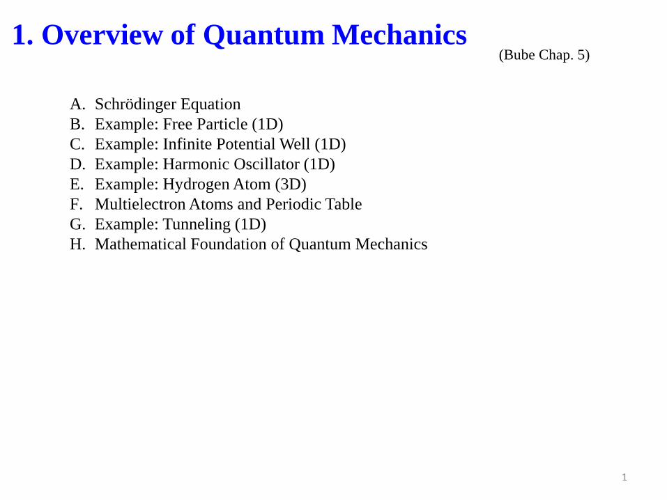
1. Overview of Quantum Mechanics
A. Schrödinger Equation
B. Example: Free Particle (1D)
C. Example: Infinite Potential Well (1D)
D. Example: Harmonic Oscillator (1D)
E. Example: Hydrogen Atom (3D)
F. Multielectron Atoms and Periodic Table
G. Example: Tunneling (1D)
H. Mathematical Foundation of Quantum Mechanics
(Bube Chap. 5)
1
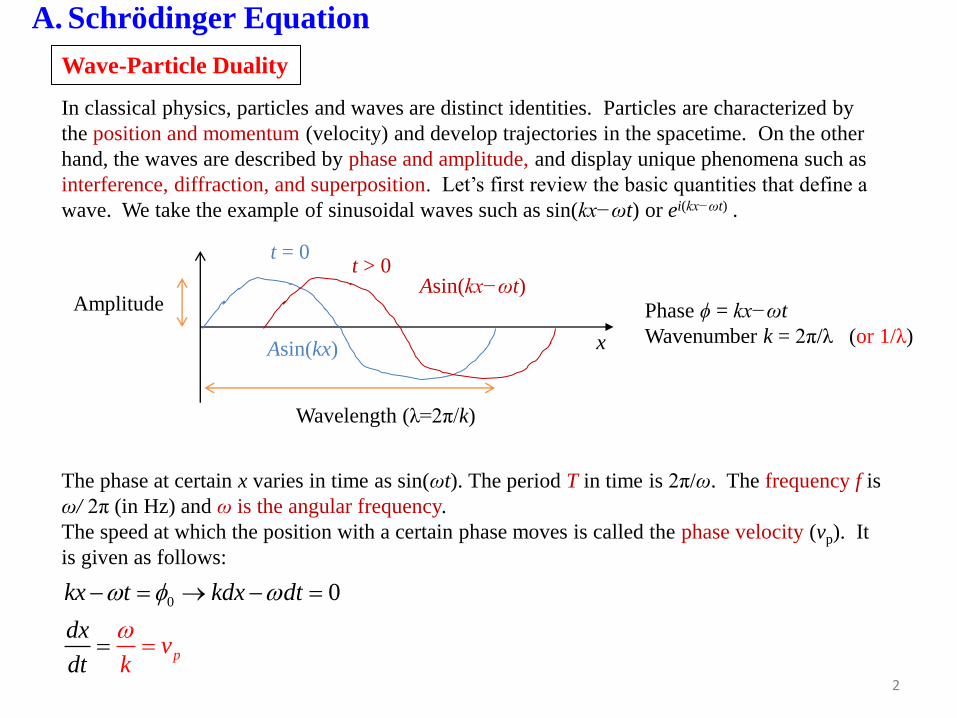
In classical physics, particles and waves are distinct identities. Particles are characterized by
the position and momentum (velocity) and develop trajectories in the spacetime. On the other
hand, the waves are described by phase and amplitude, and display unique phenomena such as
interference, diffraction, and superposition. Let’s first review the basic quantities that define a
wave. We take the example of sinusoidal waves such as sin(kx−ωt) or ei(kx−ωt) .
Wave-Particle Duality
Phase ϕ = kx−ωt
Wavenumber k = 2π/λ (or 1/λ)
The phase at certain x varies in time as sin(ωt). The period T in time is 2π/ω. The frequency f is
ω/ 2π (in Hz) and ω is the angular frequency.
The speed at which the position with a certain phase moves is called the phase velocity (vp). It
is given as follows:
t = 0
Amplitude
Wavelength (λ=2π/k)
Asin(kx)
t > 0Asin(kx−ωt)
0 0
p
kx t kdx d
xv
k
t
d
dt
− = →
= =
− =
A. Schrödinger Equation
x
2

It was Planck (1900) who first noticed the wave-particle
duality. He discovered from the research on blackbody
radiation that the energy of light waves with angular
frequency ω (=2πf) is quantized by ħω (= hf or hν), where ħ is
the Planck constant (h = 4.1357×10⁻¹⁵ eV·s) divided by 2π.
Each quantized light is called the photon. Therefore, light is a
stream of photons. In fact, any waves oscillating with ω have
discrete energy levels separated by ħω. Einstein used the
Planck’s postulate to explain the photoelectric effect, for
which he received the Nobel prize.
One of the greatest finding in modern physics is the wave-particle duality: particles show
wave properties such as interference while the classical waves sometimes have granularity
(discreteness) of particles with certain momentum.
Light as
electromagnetic
waves
Light as a
stream of
photons
3
The emission of electrons
from a metal plate caused by
light quanta – photons.
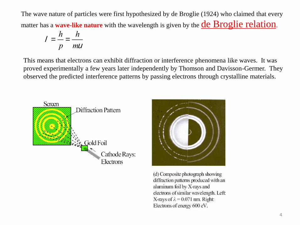
The wave nature of particles were first hypothesized by de Broglie (1924) who claimed that every
matter has a wave-like nature with the wavelength is given by the de Broglie relation.
l =h
p=
h
mu
This means that electrons can exhibit diffraction or interference phenomena like waves. It was
proved experimentally a few years later independently by Thomson and Davisson-Germer. They
observed the predicted interference patterns by passing electrons through crystalline materials.
4
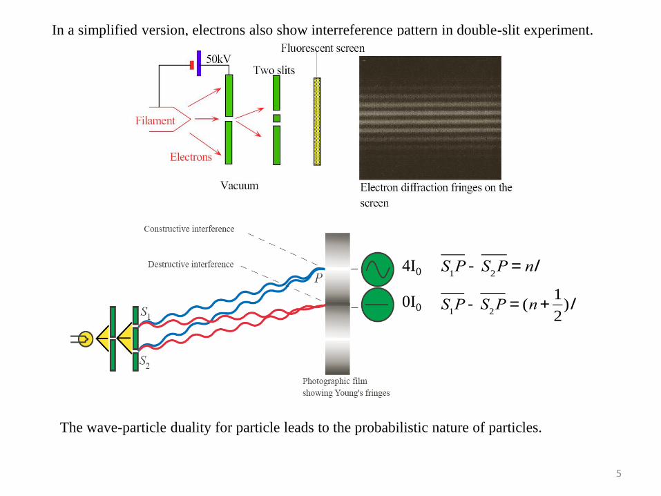
4I0
0I0
S
1P - S
2P = nl
S
1P - S
2P = (n +
1
2)l
In a simplified version, electrons also show interreference pattern in double-slit experiment.
The wave-particle duality for particle leads to the probabilistic nature of particles.
5
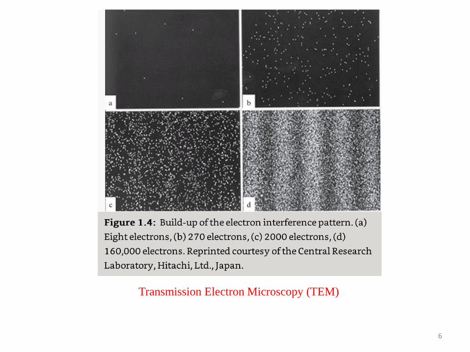
Transmission Electron Microscopy (TEM)
6
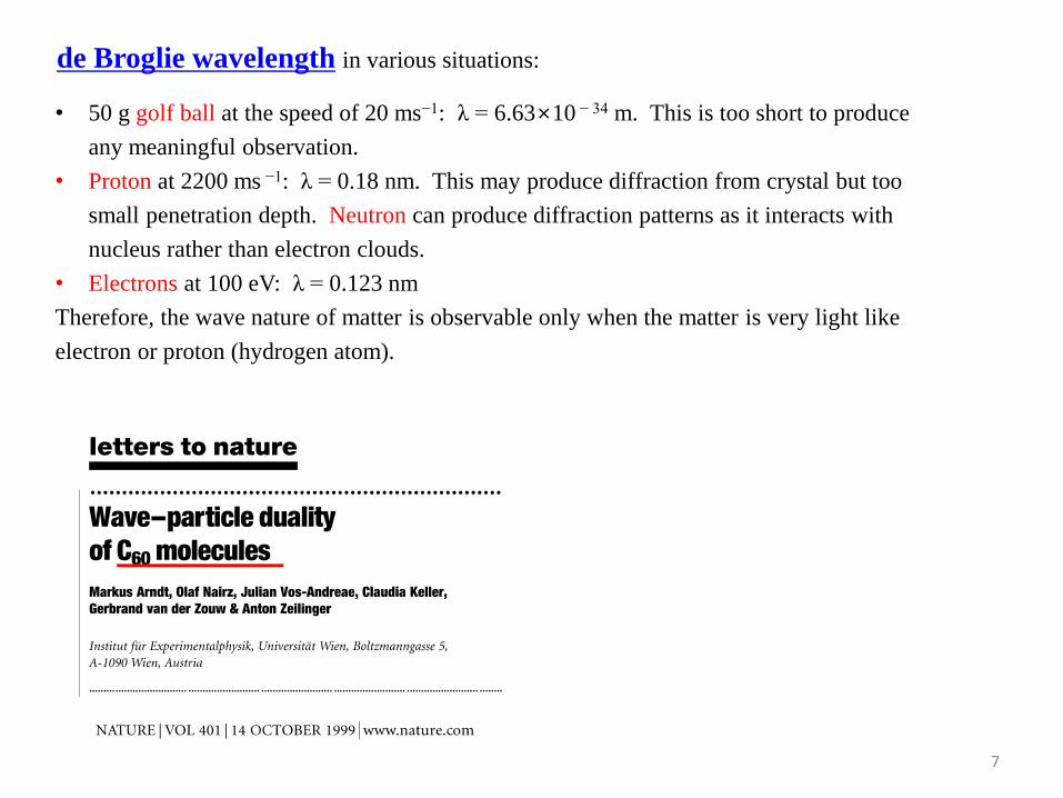
• 50 g golf ball at the speed of 20 ms−1: λ = 6.63×10 − 34 m. This is too short to produce
any meaningful observation.
• Proton at 2200 ms −1: λ = 0.18 nm. This may produce diffraction from crystal but too
small penetration depth. Neutron can produce diffraction patterns as it interacts with
nucleus rather than electron clouds.
• Electrons at 100 eV: λ = 0.123 nm
Therefore, the wave nature of matter is observable only when the matter is very light like
electron or proton (hydrogen atom).
de Broglie wavelength in various situations:
7
_______
Schrödinger Equation
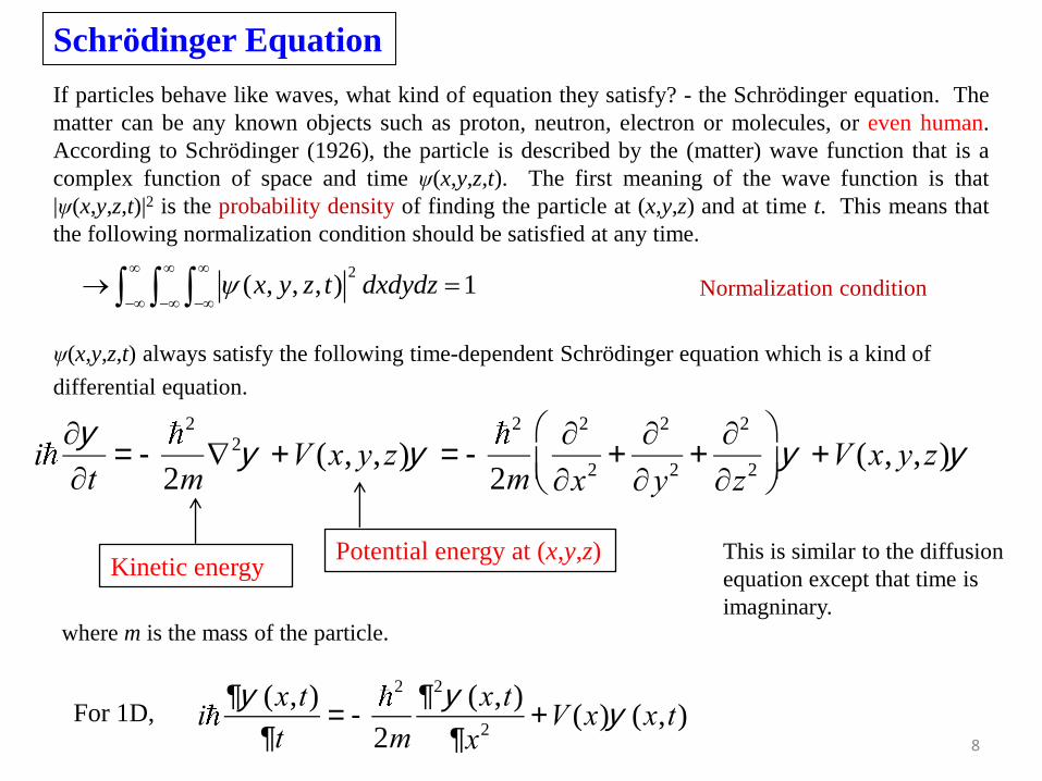
ψ(x,y,z,t) always satisfy the following time-dependent Schrödinger equation which is a kind of
differential equation.
i¶y
¶t= -
2
2mÑ2y +V (x, y,z)y = -
2
2m
¶2
¶x2+
¶2
¶y2+¶2
¶z2
æ
èç
ö
ø÷y +V (x, y,z)y
Potential energy at (x,y,z)
For 1D,
i
¶y (x,t)
¶t= -
2
2m
¶2y (x,t)
¶x2+V (x)y (x,t)
2( , , , ) 1x y z t dxdydz
− − −→ =
Kinetic energy
Normalization condition
If particles behave like waves, what kind of equation they satisfy? - the Schrödinger equation. The
matter can be any known objects such as proton, neutron, electron or molecules, or even human.
According to Schrödinger (1926), the particle is described by the (matter) wave function that is a
complex function of space and time ψ(x,y,z,t). The first meaning of the wave function is that
|ψ(x,y,z,t)|2 is the probability density of finding the particle at (x,y,z) and at time t. This means that
the following normalization condition should be satisfied at any time.
where m is the mass of the particle.
This is similar to the diffusion
equation except that time is
imagninary.
8

There are mathematical conditions that should be satisfied by the wave functions: single-valued,
function and first derivatives are continuous
(At the point where V diverges, the first derivative can be discontinuous.)
Superposition principle: Since the Schrodinger equation is linear, if ψ1 and ψ2 are solutions to
the Schrodinger equation, ψ1+ ψ2 is also a valid solution.
9
No kinks in natureNot in nature

( , , , ) ( , , ) ( , , )E
i ti tx y z t x y z e x y z e
−−= =
-
2
2m
d 2
dx2y (x) +Vy (x) = Ey (x)
This is called time-independent Schrödinger equation or simply Schrödinger equation. Note that this
is mathematically an eigenvalue problem. With proper boundary conditions, the solution to this
equation produces a set of energy eigenvalues and corresponding energy eigenstates.
E: total energy = ħω
(similar to photon)
A special solution is the steady state or constant-energy state for which
In this special case, the time-dependent Schrödinger equation becomes time-independent as follows:
For 1D,
10
________________
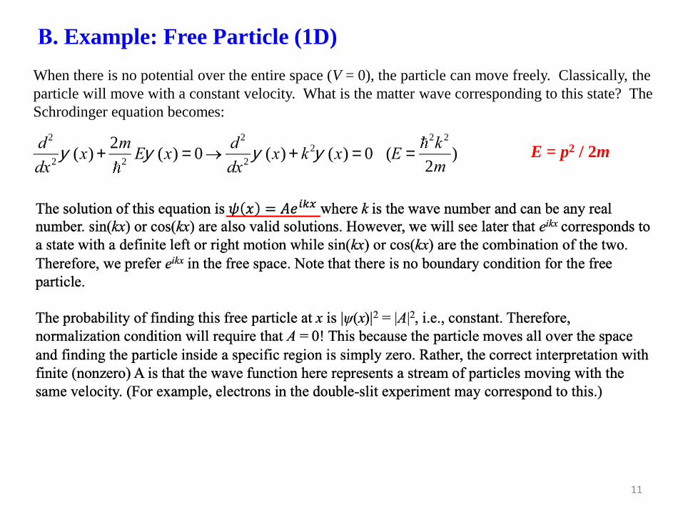
Β. Example: Free Particle (1D)
d 2
dx2y (x) +
2m2
Ey (x) = 0®d 2
dx2y (x) + k 2y (x) = 0 (E =
2k 2
2m)
When there is no potential over the entire space (V = 0), the particle can move freely. Classically, the
particle will move with a constant velocity. What is the matter wave corresponding to this state? The
Schrodinger equation becomes:
11
___________
E = p2 / 2m
y (x,t) =y (x)e- i
Et
= Aei(kx-wt )
The full wave function ψ(x,t) is given by
Wavelength λ = 2π/k. According to the de Broglie relation, λ = h/p. Therefore, p = ħk. This is
consistent with
In addition,
Such relation between frequency and wavenumber (ω=ω(k)) is called the dispersion relation .
For the light or photons, ω = ck.
12
ppt 1-10
Free Particle (1D)______
_____
Dispersion Relation: electron, phonon, photon, etc.
ex. Free electron model
v
g=
dw
dk=
k
m=
p
m
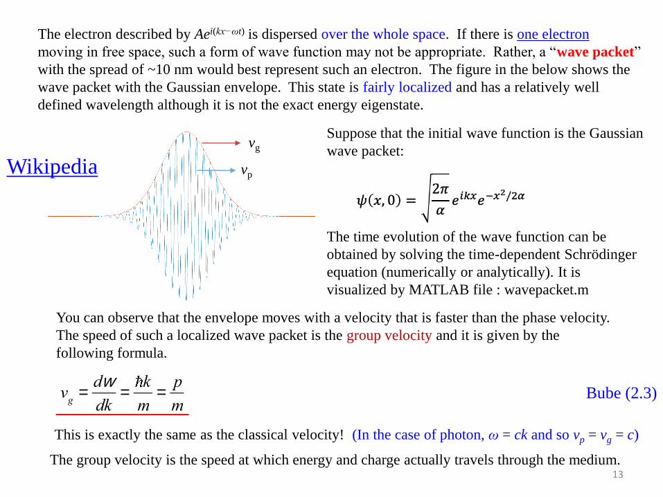
The electron described by Aei(kx−ωt) is dispersed over the whole space. If there is one electron
moving in free space, such a form of wave function may not be appropriate. Rather, a “wave packet”
with the spread of ~10 nm would best represent such an electron. The figure in the below shows the
wave packet with the Gaussian envelope. This state is fairly localized and has a relatively well
defined wavelength although it is not the exact energy eigenstate.
You can observe that the envelope moves with a velocity that is faster than the phase velocity.
The speed of such a localized wave packet is the group velocity and it is given by the
following formula.
This is exactly the same as the classical velocity! (In the case of photon, ω = ck and so vp = vg = c)
Suppose that the initial wave function is the Gaussian
wave packet:
The time evolution of the wave function can be
obtained by solving the time-dependent Schrödinger
equation (numerically or analytically). It is
visualized by MATLAB file : wavepacket.m
vg
vp
The group velocity is the speed at which energy and charge actually travels through the medium.13
Bube (2.3) ________________
Wikipedia
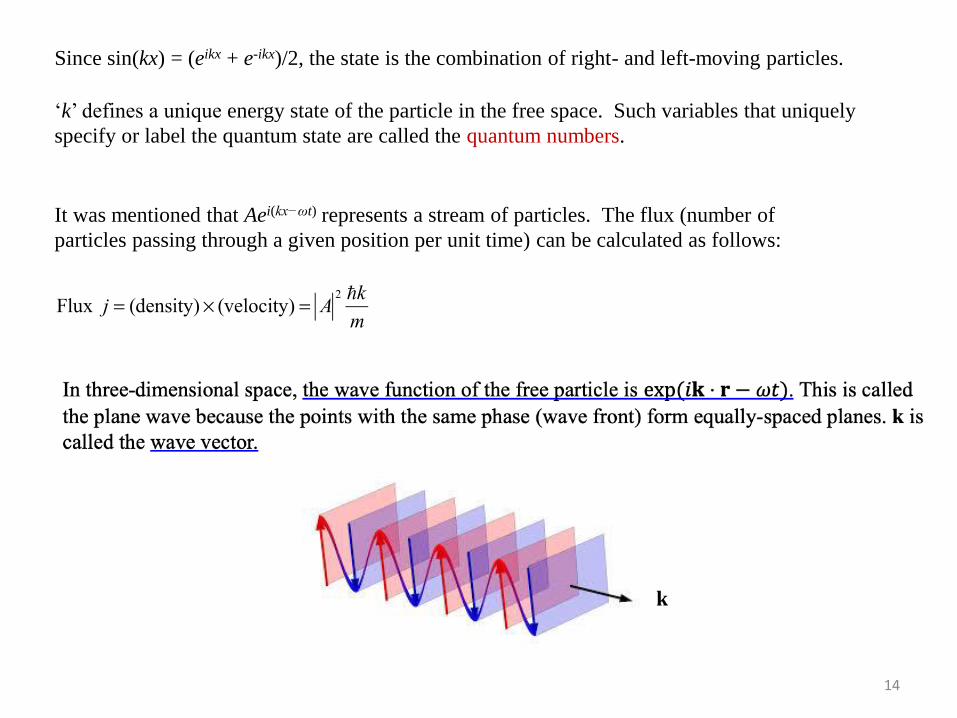
‘k’ defines a unique energy state of the particle in the free space. Such variables that uniquely
specify or label the quantum state are called the quantum numbers.
Since sin(kx) = (eikx + e-ikx)/2, the state is the combination of right- and left-moving particles.
It was mentioned that Aei(kx−ωt) represents a stream of particles. The flux (number of
particles passing through a given position per unit time) can be calculated as follows:
k
14
_________________________________________
_________
-
2
2m
d 2
dx2y (x) = Ey (x)®
d 2
dx2y (x) +
2m2
Ey (x) = 0
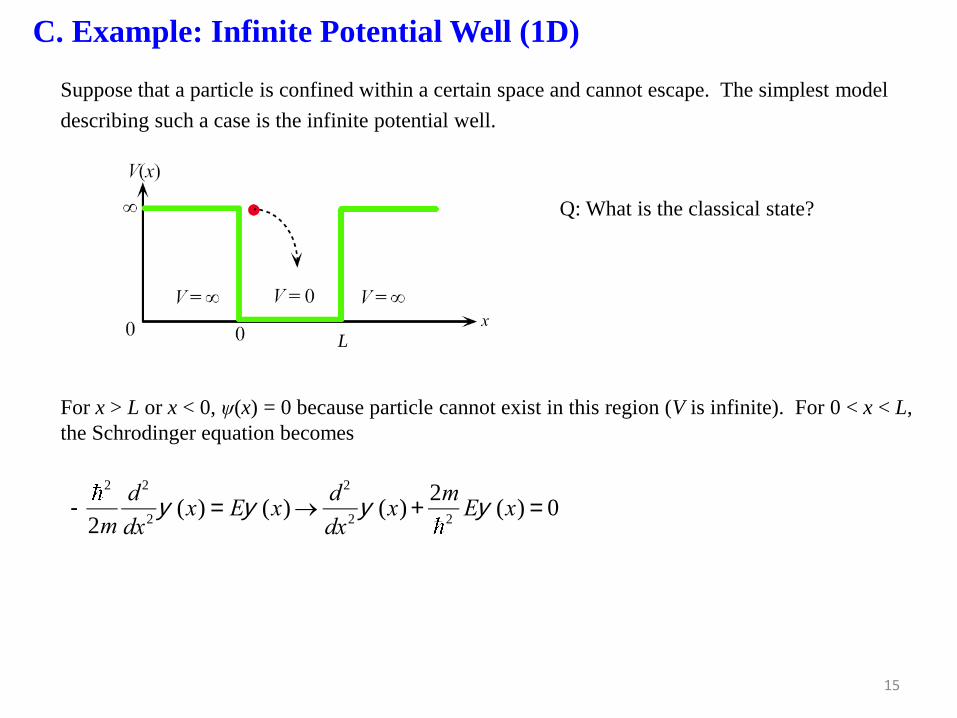
C. Example: Infinite Potential Well (1D)
Q: What is the classical state?
Suppose that a particle is confined within a certain space and cannot escape. The simplest model
describing such a case is the infinite potential well.
For x > L or x < 0, ψ(x) = 0 because particle cannot exist in this region (V is infinite). For 0 < x < L,
the Schrodinger equation becomes
L
15
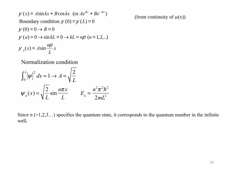
y (x) = Asin kx + Bcoskx (or Aeikx + Be- ikx )
Boundary condition y (0) =y (L) = 0
y (0) = 0® B = 0
y (a) = 0® sin kL = 0® kL = np (n = 1,2,..)
yn(x) = Asin
np
Lx
(from continuity of ψ(x))
Since n (=1,2,3…) specifies the quantum state, it corresponds to the quantum number in the infinite
well.
16

17

Bound state (localized state)
Ground state (n=1)
1st excited state (n=2)
2nd excited state (n=3)
L L
L
(Note that ψ′(x) is discontinuous at x = 0 and
L because V is infinite at those points)
18

Remarks on the solution of infinite potential well.
i) Energy is quantized. (Note that it is only kinetic energy.) Classically, energy can be any
non-negative real number. Let’s calculate the energy interval (Δε) between 1st and 2nd states.
First, a 1-kg object in a macroscopic system with L = 1 m, Δε ~ 10−67 J ~ 10−48 eV. This is too
small energy to be observed. Therefore, the energy is effectively continuous.
Next, if the electron is confined within an atom, L is about 2 Å . In this case, Δε ~ 10 eV
which is substantial. Therefore, quantum effects (energy quantization) are expected for
electrons bound within the scale of atoms or molecules. This is also known as the quantum
confinement effect in nanoscience. (The energy was not quantized in the free particle because
the electron was not confined there.) For this reason, the nanoscale potential well is often
called the “quantum well”.
ii) “Going faster” in classical mechanics → increase n in quantum mechanics. Wavefunction is
more oscillatory with shorter wave lengths as the quantum number goes up. Therefore, shorter
wave length means higher kinetic energy. Mathematically, this is because the kinetic energy
corresponds to the second derivative of the wave functions.
iii) Probability is not uniform but effectively uniform at large n. (Q: what is the probability in
the classical mechanics?)
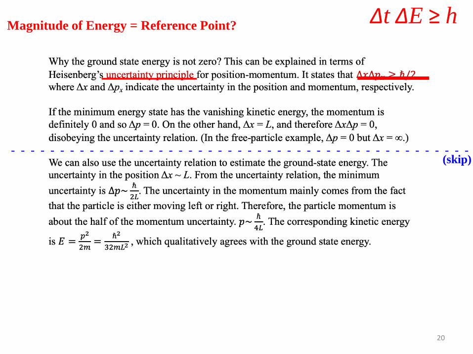
iv) There is a minimum energy (zero-point energy): see uncertainty relation.
v) Parity or symmetry: even parity for n = 1,3,5,.. & odd parity for n = 2,4,6,..
19-Tue/9/1/20
20
Magnitude of Energy = Reference Point?
________ ___
- - - - - - - - - - - - - - - - - - - - - - - - - - - - - - - - - - - - - - - - - - - - - - -(skip)
Δt ΔE ≥ h
D. Example: Harmonic Oscillator (1D)
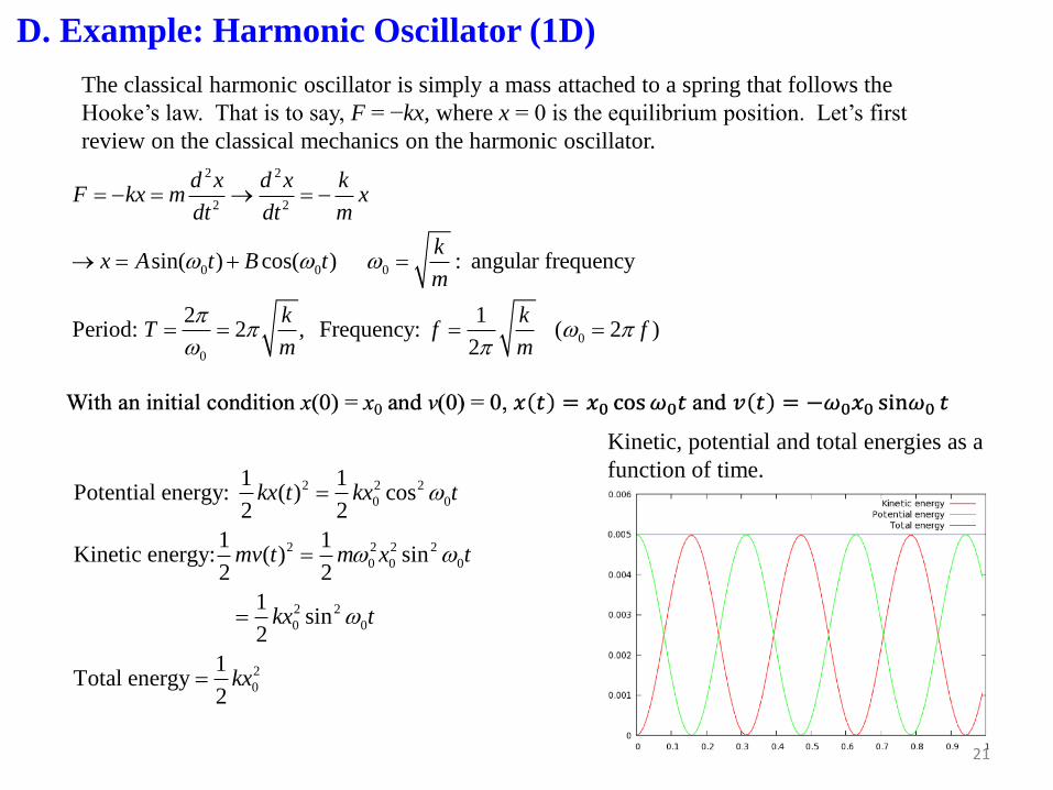
The classical harmonic oscillator is simply a mass attached to a spring that follows the
Hooke’s law. That is to say, F = −kx, where x = 0 is the equilibrium position. Let’s first
review on the classical mechanics on the harmonic oscillator.
2 2
2 2
0 0 0
0
0
sin( ) cos( ) : angular frequency
2 1Period: 2 , Frequency: ( 2 )
2
d x d x kF kx m x
dt dt m
kx A t B t
m
k kT f f
m m
= − = → = −
→ = + =
= = = =
2 2 2
0 0
2 2 2 2
0 0 0
2 2
0 0
2
0
1 1Potential energy: ( ) cos
2 2
1 1Kinetic energy: ( ) sin
2 2
1 sin
2
1Total energy
2
kx t kx t
mv t m x t
kx t
kx
=
=
=
=
Kinetic, potential and total energies as a
function of time.
21
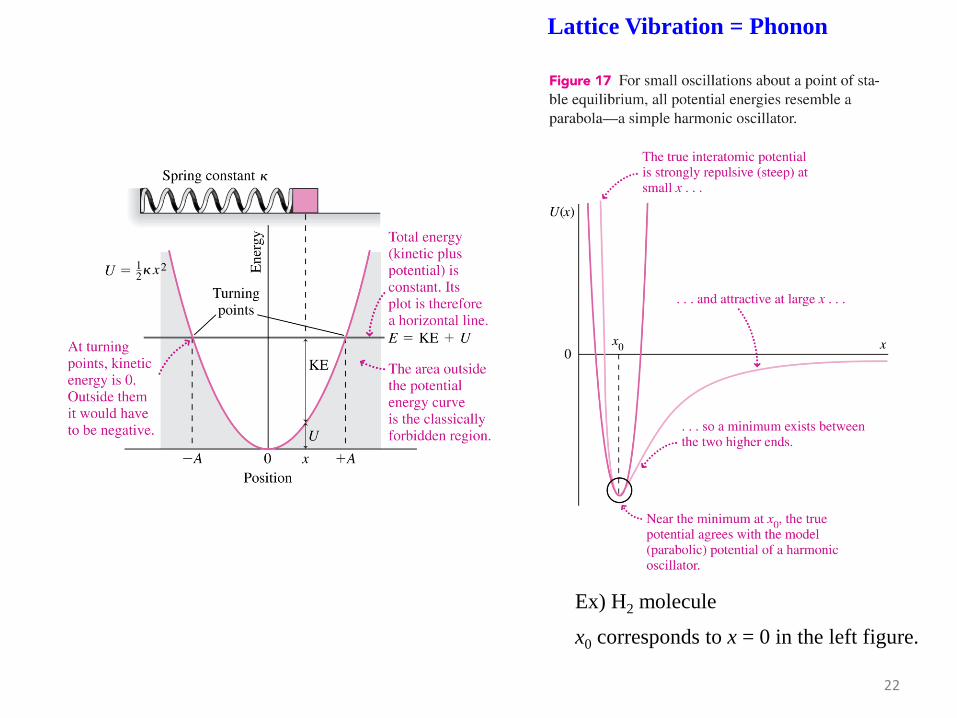
Ex) H2 molecule
x0 corresponds to x = 0 in the left figure.
22
Lattice Vibration = Phonon
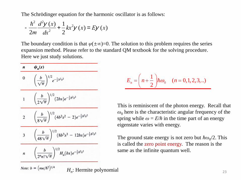
The Schrödinger equation for the harmonic oscillator is as follows:
-2
2m
d 2y (x)
dx2+
1
2kx2y (x) = Ey (x)
The boundary condition is that ψ(±∞)=0. The solution to this problem requires the series
expansion method. Please refer to the standard QM textbook for the solving procedure.
Here we just study solutions.
Hn: Hermite polynomial
0
1( 0,1,2,3,..)
2nE n n
= + =
This is reminiscent of the photon energy. Recall that
ω0 here is the characteristic angular frequency of the
spring while ω = Ε/ħ in the time part of an energy
eigenstate varies with energy.
The ground state energy is not zero but ħω0/2. This
is called the zero point energy. The reason is the
same as the infinite quantum well.
23
________________

Shorter wavelength
→ higher speed
Particle exists beyond turning points
due to the tunneling effect.24
14
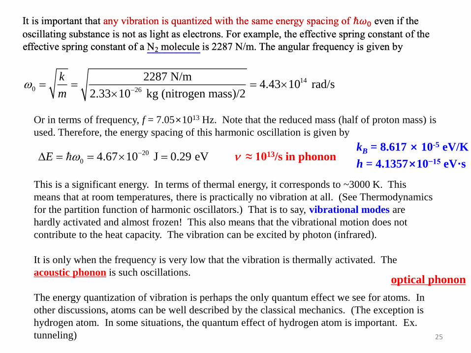
0 26
2287 N/m4.43 10 rad/s
2.33 10 kg (nitrogen mass)/2
k
m
−= = =
20
0 4.67 10 J 0.29 eVE − = = =
Or in terms of frequency, f = 7.05×10¹³ Hz. Note that the reduced mass (half of proton mass) is
used. Therefore, the energy spacing of this harmonic oscillation is given by
This is a significant energy. In terms of thermal energy, it corresponds to ~3000 K. This
means that at room temperatures, there is practically no vibration at all. (See Thermodynamics
for the partition function of harmonic oscillators.) That is to say, vibrational modes are
hardly activated and almost frozen! This also means that the vibrational motion does not
contribute to the heat capacity. The vibration can be excited by photon (infrared).
It is only when the frequency is very low that the vibration is thermally activated. The
acoustic phonon is such oscillations.
The energy quantization of vibration is perhaps the only quantum effect we see for atoms. In
other discussions, atoms can be well described by the classical mechanics. (The exception is
hydrogen atom. In some situations, the quantum effect of hydrogen atom is important. Ex.
tunneling) 25
_________
kB = 8.617 × 10⁻⁵ eV/K
h = 4.1357×10⁻¹⁵ eV·sn ≈ 1013/s in phonon
optical phonon

26
Acoustic and Optical Phonons in a Crystal
Phonon Wavevector k
n ≈ 1013/s
0
1( 0,1,2,3,..)
2nE n n
= + =
ppt 1-23
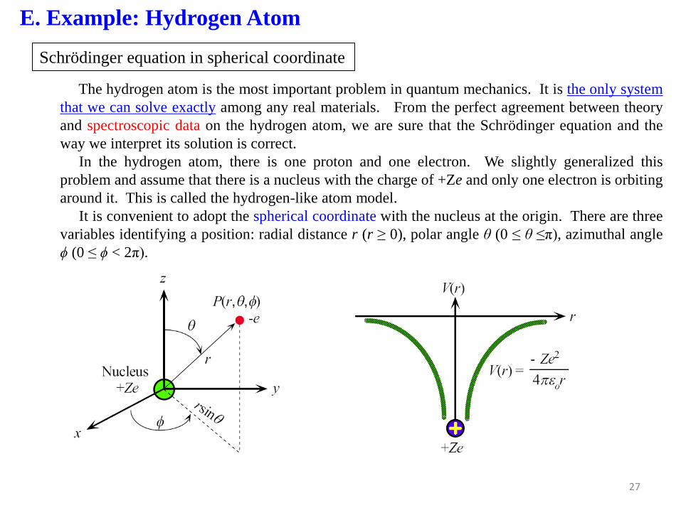
The hydrogen atom is the most important problem in quantum mechanics. It is the only system
that we can solve exactly among any real materials. From the perfect agreement between theory
and spectroscopic data on the hydrogen atom, we are sure that the Schrödinger equation and the
way we interpret its solution is correct.
In the hydrogen atom, there is one proton and one electron. We slightly generalized this
problem and assume that there is a nucleus with the charge of +Ze and only one electron is orbiting
around it. This is called the hydrogen-like atom model.
It is convenient to adopt the spherical coordinate with the nucleus at the origin. There are three
variables identifying a position: radial distance r (r ≥ 0), polar angle θ (0 ≤ θ ≤π), azimuthal angle
ϕ (0 ≤ ϕ < 2π).
Schrödinger equation in spherical coordinate
E. Example: Hydrogen Atom
27
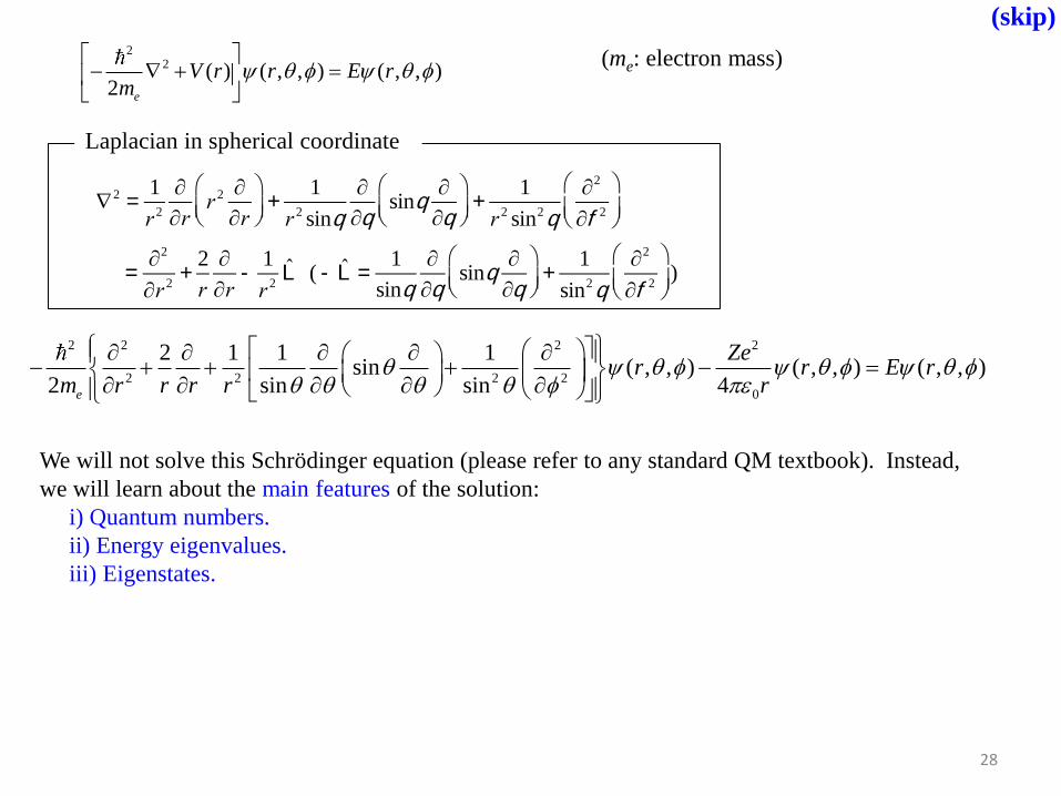
Laplacian in spherical coordinate
Ñ2 =1
r 2
¶rr 2 
¶r
æ
èçö
ø÷+
1
r 2 sinq
¶qsinq
¶q
æ
èçö
ø÷+
1
r 2 sin2q
¶2
¶f 2
æ
èç
ö
ø÷
=¶2
¶r 2+
2
r
¶r-
1
r 2L ( - L =
1
sinq
¶qsinq
¶q
æ
èçö
ø÷+
1
sin2q
¶2
¶f 2
æ
èç
ö
ø÷ )
2 2 2 2
2 2 2 2
0
2 1 1 1sin ( , , ) ( , , ) ( , , )
2 sin sin 4e
Zer r E r
m r r r r r
− + + + − =
22 ( ) ( , , ) ( , , )
2 e
V r r E rm
− + =
We will not solve this Schrödinger equation (please refer to any standard QM textbook). Instead,
we will learn about the main features of the solution:
i) Quantum numbers.
ii) Energy eigenvalues.
iii) Eigenstates.
(me: electron mass)
28
(skip)

Quantum Numbers
0
0
−1 0 1
0
−1 0 1
−1 0 1 2−2
n=1
(K shell)
n=2
(L shell)
n=3
(M shell)
ℓ=0 ℓ=1
ℓ=0
ℓ=2
ℓ=1
ℓ=0subshells
(or ↑, ↓)
0: s 1: p 2: d 3: f ...
( )
(n, ℓ, mℓ, ms)
29
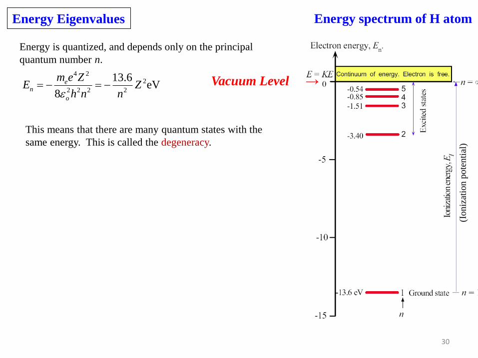
4 22
2 2 2 2
13.6eV
8
en
o
m e ZE Z
h n n= − = −
Energy spectrum of H atom
(Io
niz
atio
n p
ote
nti
al)
This means that there are many quantum states with the
same energy. This is called the degeneracy.
Energy is quantized, and depends only on the principal
quantum number n.
Energy Eigenvalues
30
Vacuum Level →
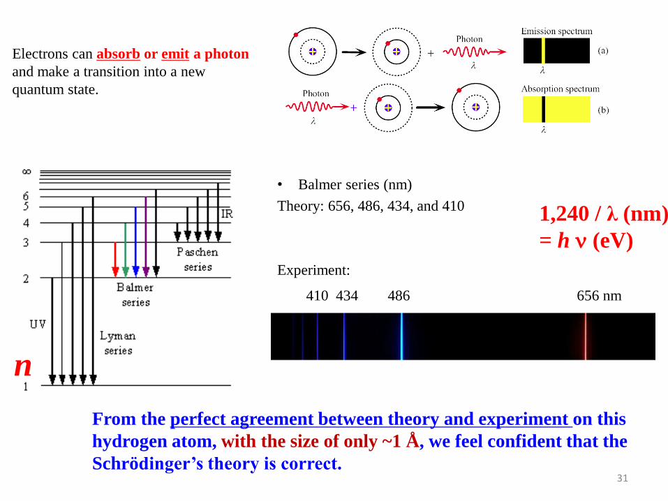
• Balmer series (nm)
Theory: 656, 486, 434, and 410
Experiment:
410 434 486 656 nm
From the perfect agreement between theory and experiment on this
hydrogen atom, with the size of only ~1 Å , we feel confident that the
Schrödinger’s theory is correct.
Electrons can absorb or emit a photon
and make a transition into a new
quantum state.
31
1,240 / λ (nm)
= h n (eV)
n
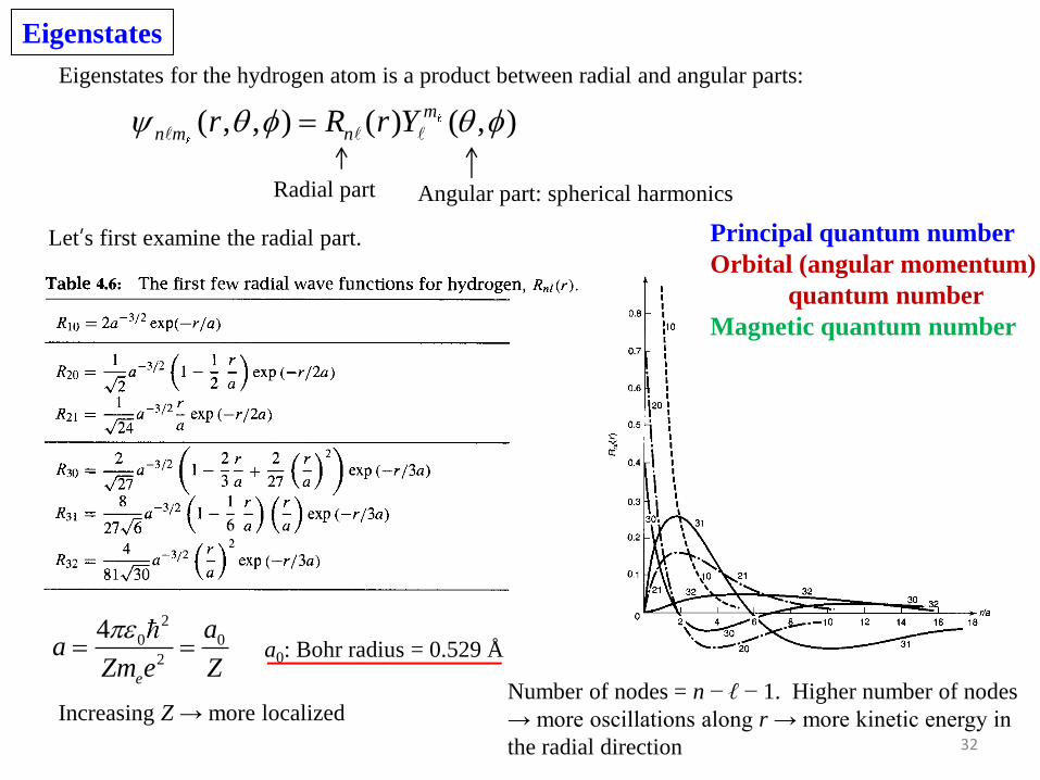
( , , ) ( ) ( , )m
n m nr R r Y =
a0: Bohr radius = 0.529 Å
Angular part: spherical harmonicsRadial part
2
0 0
2
4
e
aa
Zm e Z
= =
Eigenstates for the hydrogen atom is a product between radial and angular parts:
Number of nodes = n − ℓ − 1. Higher number of nodes
→ more oscillations along r → more kinetic energy in
the radial direction
Increasing Z → more localized
Let’s first examine the radial part.
Eigenstates
32
Principal quantum number
Orbital (angular momentum)
quantum number
Magnetic quantum number
__________________

• Increasing n pushes the
distribution outward.
• Electron is more localized for
higher ℓ values for the same n.
33
_
_
_
Transition Metal
ex. Co27 = [Ar]3d74s2
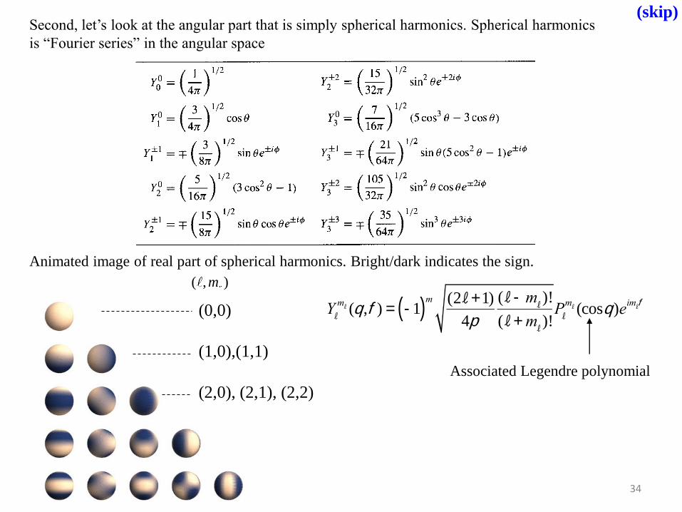
Second, let’s look at the angular part that is simply spherical harmonics. Spherical harmonics
is “Fourier series” in the angular space
Animated image of real part of spherical harmonics. Bright/dark indicates the sign.
( , )m
(0,0)
(1,0),(1,1)
(2,0), (2,1), (2,2)
Yℓ
mℓ (q ,f) = -1( )m (2ℓ+1)
4p
(ℓ- mℓ)!
(ℓ+ mℓ)!
Pℓ
mℓ (cosq )eimℓf
Associated Legendre polynomial
34
(skip)
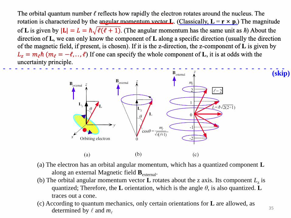
(a) The electron has an orbital angular momentum, which has a quantized component L
along an external Magnetic field Bexternal.
(b) The orbital angular momentum vector L rotates about the z axis. Its component Lz is
quantized; Therefore, the L orientation, which is the angle θ, is also quantized. L
traces out a cone.
(c) According to quantum mechanics, only certain orientations for L are allowed, as determined by and m
35
__________ ________________
(skip) - - - - - - - - - - - - - - - - - - - - - - - - - - - - - - - - - - - - - - - - - - - - - - -

When an electron in the hydrogen-like atom absorbs or emits a photon by changing its quantum
state, the transition should satisfy the Selection Rules of Δℓ = ±1 and Δm = 0, ±1. This is
because photon itself has an angular momentum with the magnitude of ħ. The figure
below shows the possible transition for emission of one photon.
36
H atom

Another representation of p and d orbtials
0
1
1 1
1 1
1 1
1 1
cos orbital
sin ( ) sin cos orbital
sin ( ) sin sin orbital
z
i i
x
i i
y
Y z p
Y Y e e x p
Y Y e e y p
− −
− −
→
+ + →
− − →
p orbital d orbital37
__
_ _
(skip)
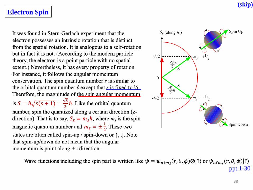
Electron Spin
38
______________________
ppt 1-30
(skip)

Magnetic Dipole Moment of Electron
Likewise, the spinning electron can be imagined to be
equivalent to a current loop. This current loop behaves
like a bar magnet, just as in the orbital case. This
produces the spin magnetic moment (μspin).
The orbiting electron is equivalent to a current loop
that behaves like a bar magnet. The resulting
magnetic moment is called the orbital magnetic
moment (μorbital) is given by
orbital2 e
e
m= −μ L
spin
e
e
m= −μ S
The total magnetic moment is
tot orbital spin ( 2 )2 e
e
m= + = − +μ μ μ L S
We will come back to this formula when discussing on the magnetic properties. 39
(skip)
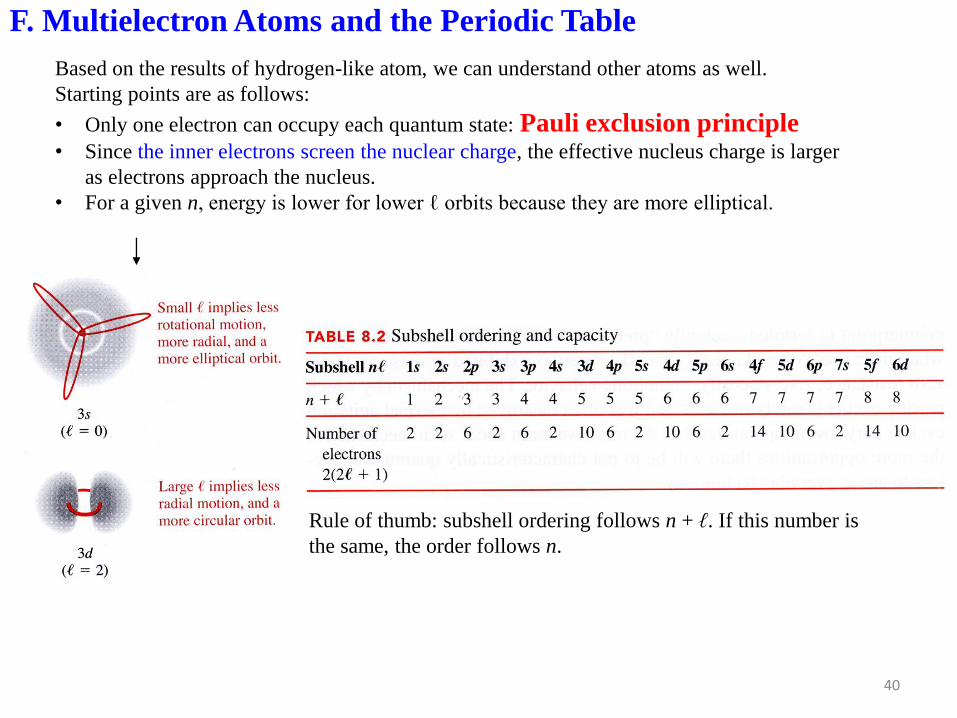
F. Multielectron Atoms and the Periodic Table
Based on the results of hydrogen-like atom, we can understand other atoms as well.
Starting points are as follows:
• Only one electron can occupy each quantum state: Pauli exclusion principle • Since the inner electrons screen the nuclear charge, the effective nucleus charge is larger
as electrons approach the nucleus.
• For a given n, energy is lower for lower ℓ orbits because they are more elliptical.
Rule of thumb: subshell ordering follows n + ℓ. If this number is
the same, the order follows n.
40
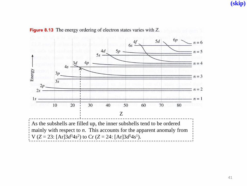
As the subshells are filled up, the inner subshells tend to be ordered
mainly with respect to n. This accounts for the apparent anomaly from
V (Z = 23: [Ar]3d34s2) to Cr (Z = 24: [Ar]3d54s1).
Z
41
(skip)
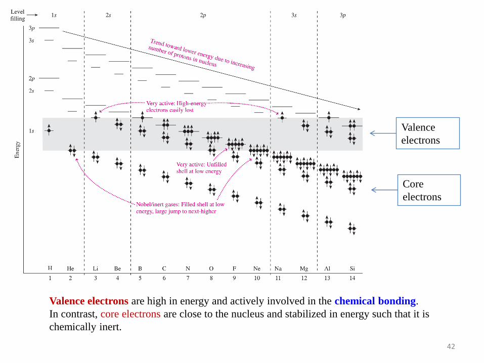
Valence
electrons
Core
electrons
Valence electrons are high in energy and actively involved in the chemical bonding.
In contrast, core electrons are close to the nucleus and stabilized in energy such that it is
chemically inert.
42
• He: the 1s electrons are too tightly bound with large energy so it does not engage in
chemical reactions. → Noble gas. 1s shell in He is closed.
• Li: high energy electron is easily lost.
• Be: 2s subshell is filled. However, since its energy is relatively high, it is still chemically
active.
• B, C, N: electrons in 2p subshell favors high-spin configuration : Hund’s rule (principle of
maximum spin multiplicity)– main origin is the reduction in screening of nuclear charges
by occupying different orbitals + exchange effects
• O, F, Ne: electron in the downward directions are occupied.
• B-F: 2p subshell is partially occupied and therefore chemically active
• B-N: 2s subshell, albeit filled up, is chemically active → s-p hybridization
• O, F: strongly attracts electrons (O2-, F-) → high electron affinity or electronegativity
• Ionic bonding is formed between Li and F
• Ne is inert or noble gas because closed shell is chemically inert – due to energy and wave
function range.
• Chemical behavior of Na and Li (Mg and Be) are similar. (Sizes are bigger.)
43
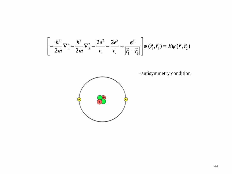
+antisymmetry condition
44
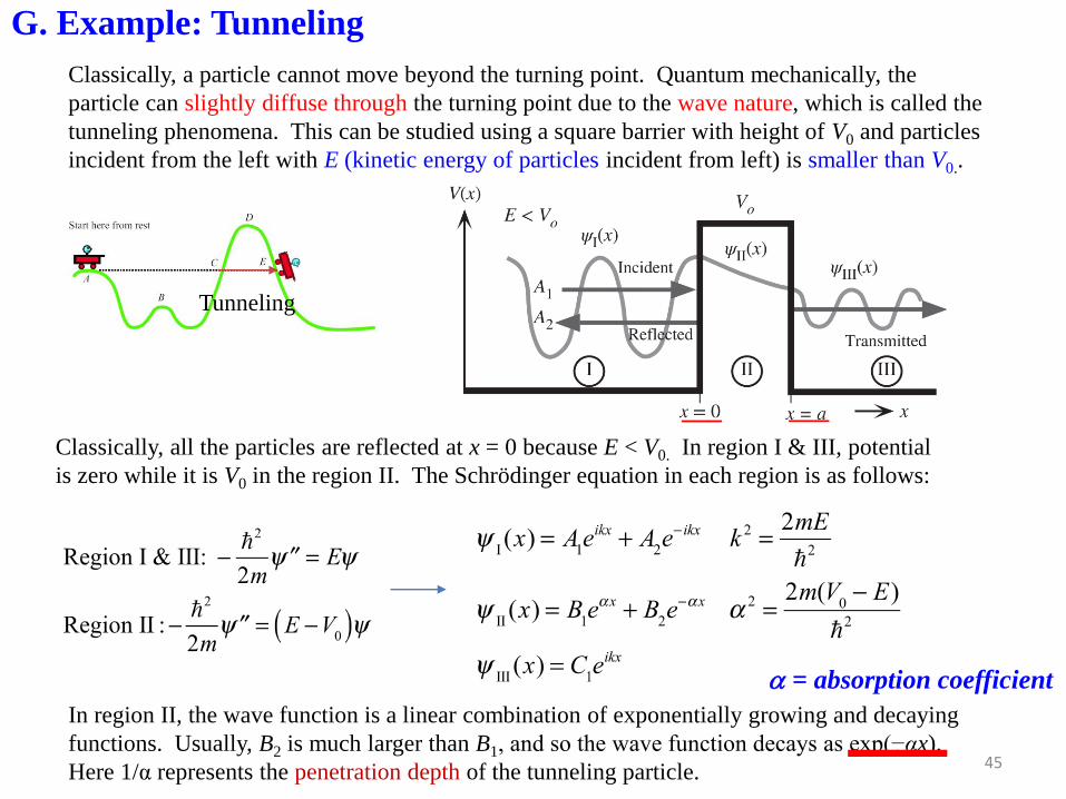
G. Example: Tunneling
Classically, a particle cannot move beyond the turning point. Quantum mechanically, the
particle can slightly diffuse through the turning point due to the wave nature, which is called the
tunneling phenomena. This can be studied using a square barrier with height of V0 and particles
incident from the left with E (kinetic energy of particles incident from left) is smaller than V0..
Tunneling
Classically, all the particles are reflected at x = 0 because E < V0. In region I & III, potential
is zero while it is V0 in the region II. The Schrödinger equation in each region is as follows:
In region II, the wave function is a linear combination of exponentially growing and decaying
functions. Usually, B2 is much larger than B1, and so the wave function decays as exp(−αx).
Here 1/α represents the penetration depth of the tunneling particle.45
___
__a = absorption coefficient
___
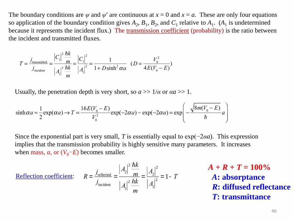
The boundary conditions are ψ and ψ′ are continuous at x = 0 and x = a. These are only four equations
so application of the boundary condition gives A2, B1, B2, and C1 relative to A1. (A1 is undetermined
because it represents the incident flux.) The transmission coefficient (probability) is the ratio between
the incident and transmitted fluxes.
Usually, the penetration depth is very short, so a >> 1/α or αa >> 1.
Since the exponential part is very small, T is essentially equal to exp(−2αa). This expression
implies that the transmission probability is highly sensitive many parameters. It increases
when mass, a, or (V0−E) becomes smaller.
Reflection coefficient:
R =jreflected
jincident
=A
2
2 k
m
A1
2 k
m
=A
2
2
A1
2= 1- T
46
A + R + T = 100%
A: absorptance
R: diffused reflectance
T: transmittance

Examples of Quantum Tunneling
i) Electron spill-over in finite quantum well
V0
E < V0
Exponentially decaying tails
In solid-state, electrons feel the band-gap region as the classically forbidden area with certain energy
barrier of V0.
AlAs/GaAs superlattice
Note that as the energy goes up, the penetration depth increases because (V0−E) is
smaller.
For E > V0, unbound state will appear and energy levels are continuous (think
about free particles).
47
Conduction Band
Valence Band
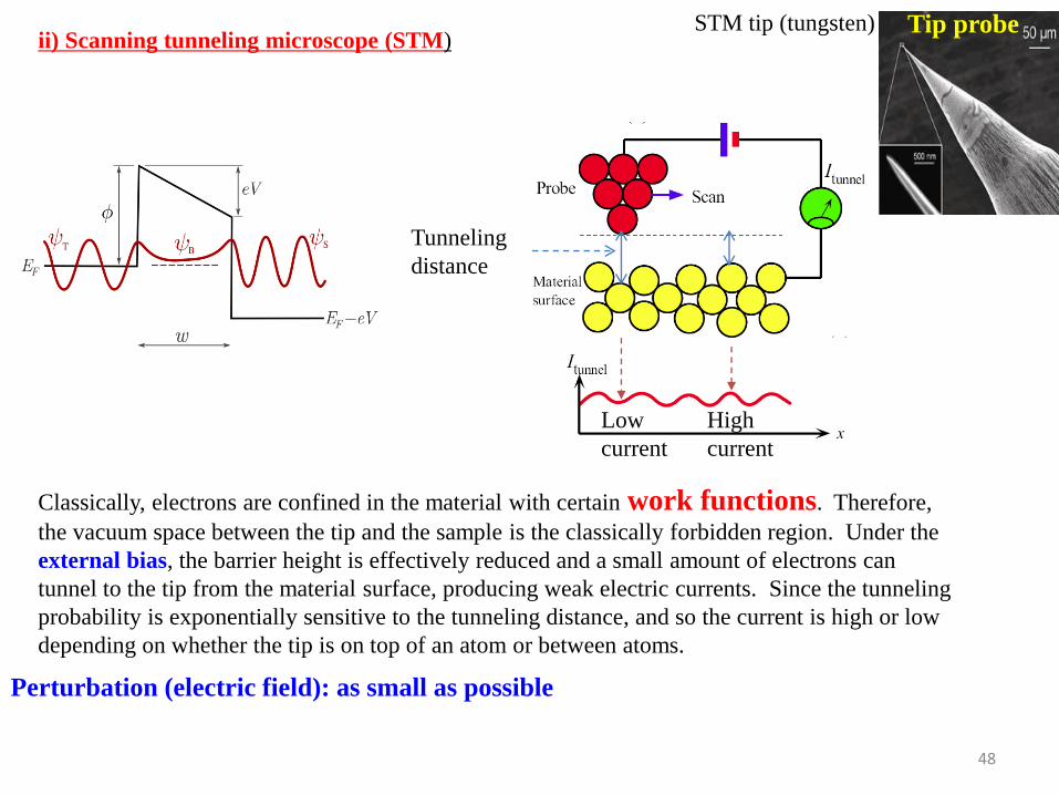
ii) Scanning tunneling microscope (STM)STM tip (tungsten)
Low
current
High
current
Classically, electrons are confined in the material with certain work functions. Therefore,
the vacuum space between the tip and the sample is the classically forbidden region. Under the
external bias, the barrier height is effectively reduced and a small amount of electrons can
tunnel to the tip from the material surface, producing weak electric currents. Since the tunneling
probability is exponentially sensitive to the tunneling distance, and so the current is high or low
depending on whether the tip is on top of an atom or between atoms.
Tunneling
distance
48
Perturbation (electric field): as small as possible
Tip probe

Graphene
Pt(111) surface
STM detects “electron cloud”
rather than atom itself.
49
Ball-and-Stick Model
Hard-Sphere Model
sp2 bond
Experiment
Experiment
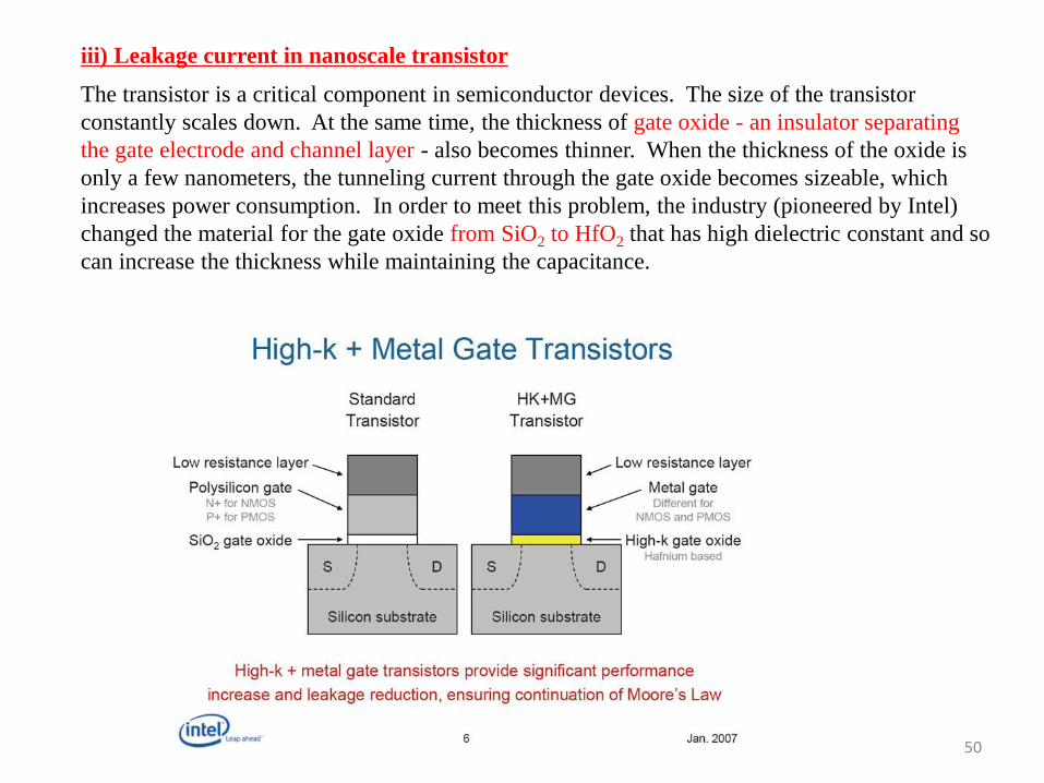
iii) Leakage current in nanoscale transistor
The transistor is a critical component in semiconductor devices. The size of the transistor
constantly scales down. At the same time, the thickness of gate oxide - an insulator separating
the gate electrode and channel layer - also becomes thinner. When the thickness of the oxide is
only a few nanometers, the tunneling current through the gate oxide becomes sizeable, which
increases power consumption. In order to meet this problem, the industry (pioneered by Intel)
changed the material for the gate oxide from SiO2 to HfO2 that has high dielectric constant and so
can increase the thickness while maintaining the capacitance.
50
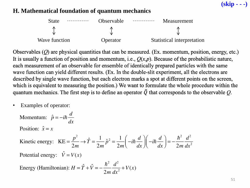
H. Mathematical foundation of quantum mechanics
State Observable Measurement
Wave function Operator Statistical interpretation
• Examples of operator:
51
(skip - - -)
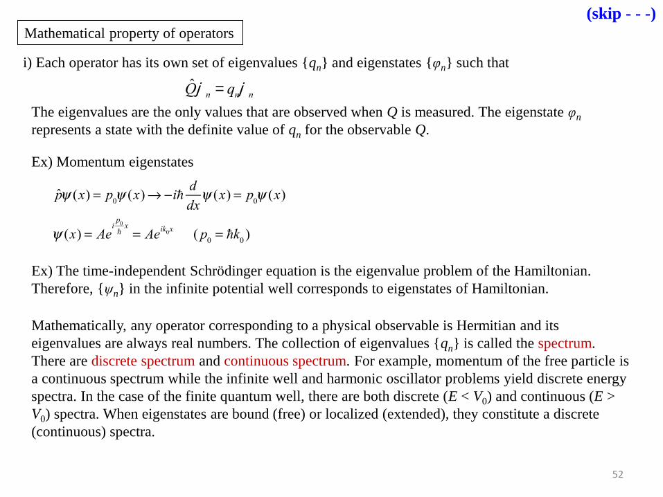
i) Each operator has its own set of eigenvalues {qn} and eigenstates {φn} such that
Qjn = qnjn
Ex) Momentum eigenstates
Ex) The time-independent Schrödinger equation is the eigenvalue problem of the Hamiltonian.
Therefore, {ψn} in the infinite potential well corresponds to eigenstates of Hamiltonian.
Mathematical property of operators
Mathematically, any operator corresponding to a physical observable is Hermitian and its
eigenvalues are always real numbers. The collection of eigenvalues {qn} is called the spectrum.
There are discrete spectrum and continuous spectrum. For example, momentum of the free particle is
a continuous spectrum while the infinite well and harmonic oscillator problems yield discrete energy
spectra. In the case of the finite quantum well, there are both discrete (E < V0) and continuous (E >
V0) spectra. When eigenstates are bound (free) or localized (extended), they constitute a discrete
(continuous) spectra.
The eigenvalues are the only values that are observed when Q is measured. The eigenstate φn
represents a state with the definite value of qn for the observable Q.
52
(skip - - -)

iii) Any wave function can be represented as a linear combination of eigenstates (completeness).
Mathematically, eigenstates can expand any function in the Hilbert space.
y (x) = anjn
n
å an = jn
*(x)y (x)dx-¥
¥
ò
ii) Eigenstates are orthonormal to each other
jn
*(x)jm(x)dx-¥
¥
ò = dn,m
Ex) Eigenstates in infinite quantum well
2
Lsin
np x
Lsin
mp x
Ldx
0
L
ò = dn,m
(δn,m: Kronecker delta)
y *yò = an
*jn
*amj
mòm
ån
å = an
*am
jn
*jmò
m
ån
å = an
2
n
å = 1
Cf. For continuous spectra, Dirac orthonormality holds: j p
* (x)jq(x)dx-¥
¥
ò = d (p - q)
53
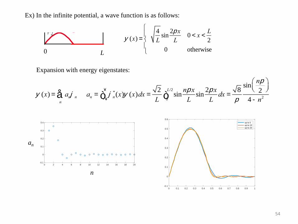
Ex) In the infinite potential, a wave function is as follows:
0 L
y (x) =
4
Lsin
2p x
L0 < x <
L
2
0 otherwise
ì
íï
îï
Expansion with energy eigenstates:
y (x) = anjn
n
å an = jn
*(x)y (x)dx-¥
¥
ò =2
Lsin
np x
Lsin
2p x
Ldx
0
L/2
ò =8
p
sinnp
2
æ
èçö
ø÷
4 - n2
0 2 4 6 8 10 12 14 16 18 20-0.1
0
0.1
0.2
0.3
0.4
0 0.1 0.2 0.3 0.4 0.5 0.6 0.7 0.8 0.9 1-0.1
0
0.1
0.2
0.3
0.4
0.5
0.6
up to 5
up to 10
up to 20
n
an
54
Q = y *Qyò = an
*jn
*Qamj
mòm
ån
å = an
*amq
mj
n
*jmò
m
ån
å = qn
an
2
n
å
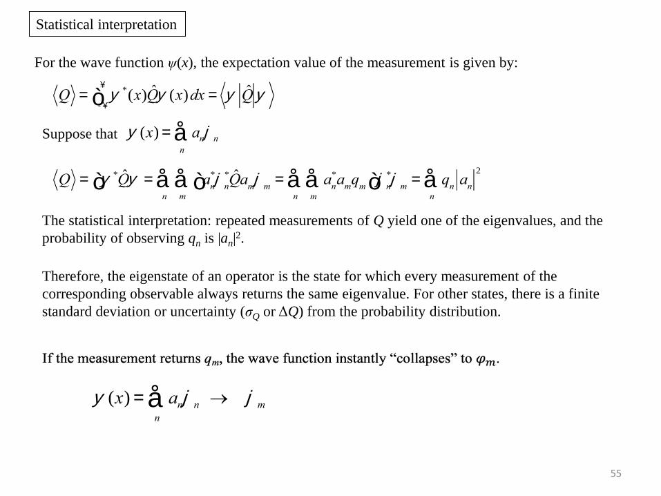
For the wave function ψ(x), the expectation value of the measurement is given by:
Q = y *(x)Qy (x)dx-¥
¥
ò = y Qy
Statistical interpretation
Suppose that y (x) = anjn
n
å
The statistical interpretation: repeated measurements of Q yield one of the eigenvalues, and the
probability of observing qn is |an|2.
Therefore, the eigenstate of an operator is the state for which every measurement of the
corresponding observable always returns the same eigenvalue. For other states, there is a finite
standard deviation or uncertainty (σQ or ΔQ) from the probability distribution.
y (x) = anjn
n
å ® jm
55
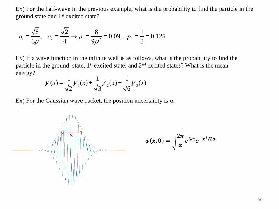
Ex) If a wave function in the infinite well is as follows, what is the probability to find the
particle in the ground state, 1st excited state, and 2nd excited states? What is the mean
energy?
y (x) =1
2y
1(x) +
1
3y
2(x) +
1
6y
3(x)
Ex) For the half-wave in the previous example, what is the probability to find the particle in the
ground state and 1st excited state?
a1 =8
3p, a2 =
2
4® p1 =
8
9p 2= 0.09, p2 =
1
8= 0.125
Ex) For the Gaussian wave packet, the position uncertainty is α.
α
56
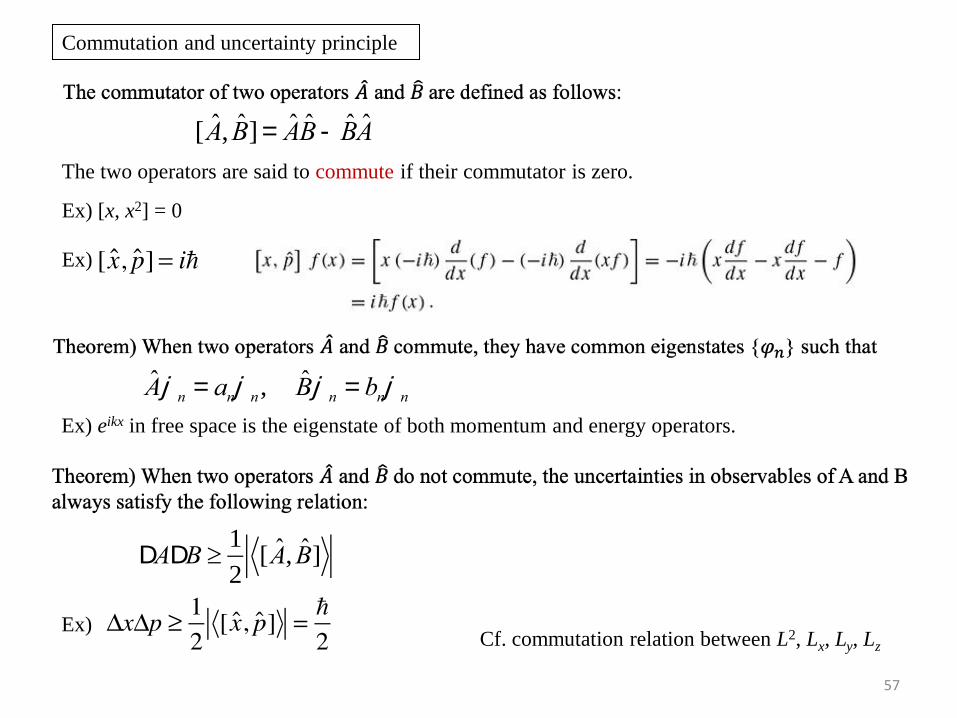
Commutation and uncertainty principle
[A, B] = AB - BA
The two operators are said to commute if their commutator is zero.
Ex) [x, x2] = 0
Ajn = anjn, Bjn = bnjn
Ex) eikx in free space is the eigenstate of both momentum and energy operators.
Ex)
DADB ³1
2[A, B]
Ex)Cf. commutation relation between L2, Lx, Ly, Lz
57
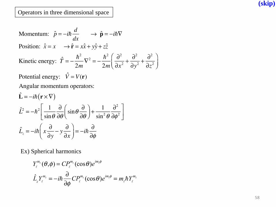
Operators in three dimensional space
Ex) Spherical harmonics
58
(skip)

Problems from Chap. 1
5-22
5-25
5-26
59-Thu/9/3/20
Related Documents