1 On Single-look Multivariate G Distribution for PolSAR Data Salman Khan, Student Member, IEEE, and Raffaella Guida, Member, IEEE Abstract For many applications where High Resolution (HR) Synthetic Aperture Radar (SAR) images are required, like urban structures detection, road map detection, marine structures and ship detection etc., single-look processing of SAR images may be desirable. The G family of distributions have been known to fit homogeneous to extremely heterogeneous Polarimetric SAR (PolSAR) data very well and can be very useful for processing single-look images. The multi-look polarimetric G distribution has a limitation that it does not reduce to single-look form for (multivariate) PolSAR data. This paper presents the new single-look polarimetric G distribution, which reduces to its two well-known special forms, the single- look K p and G 0 p distributions, when the domain of its parameters are restricted. The significance of this distribution becomes evident as it fits X- & S-band sub-meter resolution (< 1m 2 ) PolSAR data (acquired over the same scene at the same time in X- & S-bands) better than the G 0 p & K p distributions, while it fits the X-band decameter resolution (≈ 10m 2 ) PolSAR data as good as the G 0 p distribution. Numerical Maximum Likelihood Estimation (MLE) method for parameter estimation of multivariate G, G 0 p , and K p distributions is proposed. Simulated PolSAR data has been generated to validate the convergence and accuracy of maximum likelihood parameter estimates to values corresponding to globally maximum likelihood. A new iterative algorithm for accurate estimation of speckle covariance matrix is also proposed. Index Terms radar polarimetry, synthetic aperture radar, data models I. I NTRODUCTION Statistical models have been widely used for Synthetic Aperture Radar (SAR) data analysis as these data are inherently probabilistic. These models offer a wide variety of applications

Welcome message from author
This document is posted to help you gain knowledge. Please leave a comment to let me know what you think about it! Share it to your friends and learn new things together.
Transcript
1
On Single-look MultivariateG Distribution for
PolSAR Data
Salman Khan,Student Member, IEEE,and Raffaella Guida,Member, IEEE
Abstract
For many applications where High Resolution (HR) SyntheticAperture Radar (SAR) images are
required, like urban structures detection, road map detection, marine structures and ship detection etc.,
single-look processing of SAR images may be desirable. TheG family of distributions have been known
to fit homogeneous to extremely heterogeneous PolarimetricSAR (PolSAR) data very well and can be
very useful for processing single-look images. The multi-look polarimetricG distribution has a limitation
that it does not reduce to single-look form for (multivariate) PolSAR data. This paper presents the new
single-look polarimetricG distribution, which reduces to its two well-known special forms, the single-
look Kp andG0p
distributions, when the domain of its parameters are restricted. The significance of this
distribution becomes evident as it fits X- & S-band sub-meterresolution (< 1m2) PolSAR data (acquired
over the same scene at the same time in X- & S-bands) better than theG0p
& Kp distributions, while it
fits the X-band decameter resolution (≈ 10m2) PolSAR data as good as theG0p
distribution. Numerical
Maximum Likelihood Estimation (MLE) method for parameter estimation of multivariateG, G0p, andKp
distributions is proposed. Simulated PolSAR data has been generated to validate the convergence and
accuracy of maximum likelihood parameter estimates to values corresponding to globally maximum
likelihood. A new iterative algorithm for accurate estimation of speckle covariance matrix is also
proposed.
Index Terms
radar polarimetry, synthetic aperture radar, data models
I. INTRODUCTION
Statistical models have been widely used for Synthetic Aperture Radar (SAR) data analysis
as these data are inherently probabilistic. These models offer a wide variety of applications

2
including image classification, segmentation, filtering, and physical feature extraction.
It is well known in literature that, under certain assumptions, the complex return from a single-
look SAR image follows a zero-mean complex Gaussian distribution, which results in a Rayleigh
distributed amplitude, and an exponential distributed intensity [1]. With the recent advent of High
Resolution (HR) space-borne SARs, the complex Gaussian assumption of the return is not always
true. In particular, regions in the SAR image with high degree of heterogeneity (e.g. urban areas)
deviate from, while the homogeneous areas adhere to, the complex Gaussian assumption. As a
result new methods and techniques need to be identified for modeling such HR data.
SAR images have been consistently analysed and processed using the product model [2]. This
model proposes that, under certain assumptions, the complex return from a single-look SAR
image can be modeled as the product of zero-mean complex Gaussian distributed speckle and
a texture random variable [2]. In the case of homogeneous areas the texture random variable
is considered a constant which leads to a Rayleigh distributed amplitude and an exponentially
distributed intensity. In contrast to this, for heterogeneous areas the texture can be modeled
by some Probability Density Function (PDF). The choice of PDF depends on the degree of
heterogeneity of the image area, and various PDFs have thus been proposed to model texture.
These include Gamma, inverse Gaussian, Generalized Inverse Gaussian (GIG), inverse Gamma,
Beta, and Fisher distributions among others [3]–[6]. When the texture variable is Gamma,
reciprocal of Gamma, Fisher distributed the observed signal follows the K, G, Kummer-U
distributions, respectively [3]–[6]. This paper deals with a particular family of distributions of
the returned signal called theG family of distributions, which are obtained by assuming a GIG
distributed texture [5], [6]. The univariate-complex, -amplitude and -intensityG distributions
have been derived and analysed in [5]. It is important to notehere that theG0I distribution,
derived in [5], is the same as the Fisher distribution, except that the former was derived for
the return [5] while the latter was proposed for modeling thebackscatter [4]. The multivariate
(polarimetric) extension of theG distribution for multi-look PolSAR images has been presented
in [6]. A detailed bibliography of texture PDFs and the resulting distributions of the return signal
can be obtained in [7].
Many applications of SAR imagery require Very HR (VHR) data.This is usually dictated by
the size of the target to be detected. Some of the most prominent application areas where VHR
data are essential are urban structures detection [8], roadmap detection [9], marine structures

3
and ship detection [10] etc. For such applications single look complex data with the highest
possible spatial resolution are essential and multi-looking is not an option. Single-look images,
thus, need to be processed and analysed. Unfortunately, themathematical basis on which the
multi-look polarimetricG distribution has been derived does not hold for the special case of
single-look PolSAR data. In this paper, the single-look polarimetricG distribution is presented
to fill this gap. The single-look polarimetricKp andG0p distributions, listed in Table I in [11],
resulting from Gamma and reciprocal of Gamma distributed texture, are the two special forms
of the single-look polarimetricG distribution, as shown in section IV.
The utility of G distribution is demonstrated by fittingG, G0p , & Kp to amplitude histograms
of sub-meter resolution X- & S-band PolSAR data, and also to decameter resolution X-band
PolSAR data for homogeneous, moderately heterogeneous, and extremely heterogeneous areas.
The sub-meter resolution X- & S-band data have been acquiredover the same scene at the
same time. Further, a scheme to numerically estimate parameters of multivariate distributions
using Maximum Likelihood Estimation (MLE) is proposed. This scheme is also compared to
the estimation method proposed in [6], which averages MLEs of univariate (single channel)
distributions to find multivariate MLEs. Further, PolSAR data has been simulated using GIG
Gaussian texture and zero-mean complex Gaussian speckle. The convergence of numerical MLE
to global maxima and the validation of Maximum Likelihood Parameter Estimates (MLEs) has
been done using simulated PolSAR data. Also, a new iterativealgorithm for accurate estimation
of speckle covariance matrix is proposed.
The paper is organized as follows: Section II presents the speckle statistics of SAR images,
elaborates the product model describing the modeling of speckle noise and texture, and also
explains the estimation of speckle covariance matrix and the limitation of the multi-look model;
Section III introduces the GIG distribution and proves its two special forms, the Gamma and
reciprocal of Gamma distributions; Section IV presents thesingle-look polarimetricG distribu-
tion and its two special forms,Kp and G0p ; Section V explains parameter estimation of these
distributions, the speckle covariance matrix estimation algorithm and the convergence/validation
of MLEs using simulated PolSAR data; Section VI contains theapplication of the proposed
distributions to X- & S-band sub-meter resolution and X-band decameter resolution real PolSAR
data; finally, Section VII summarises the conclusions and future work.
4
II. POLARIMETRIC SAR SPECKLE STATISTICS
SAR images are characterized by a granular pattern called speckle. Speckle appears when
electromagnetic waves, emitted by a coherent source, illuminate a surface with many elementary
scatterers causing the reflected wavelets from each of thesescatterers to reach back at the point of
observation with different delays [12]. These de-phased wavelets interfere constructively at some
points and destructively at others, depending on the surface and the geometry of observation,
resulting in chaotic bright and dark spots, and also intermediate levels of brightness in the final
SAR image.
Speckle appears very unordered with no obvious relationship with the macroscopic features of
the surface and is best described by statistical methods. Inorder to understand the information
content in SAR images, it is therefore essential to study their speckle characteristics.
A. Product Model
The product model suggests that the observed speckle is composed of a product of two
statistically independent random variables; the square root of a positive random variable (scene
backscattering intensity texture)X and the speckle noiseY . The former is generally considered
to be a positive real number whereas the latter may either be complex if the SAR image is in
complex format or positive real if the image is in amplitude format. For polarimetric SAR, the
speckle noise random variable is ap-dimensional vector Yp, wherep = 3 for a mono-static SAR
and p = 4 for a bi-static configuration. For the mono-static case thep-dimensional complex
observation vector, Zp, can be represented as:
Zp =[
Shh
√2Shv Svv
]T
(1)
whereShh, Shv, andSvv are the complex polarimetric channels andSxy hasx as transmit andy
as receive electromagnetic polarization (h-horizontal,v-vertical). In terms of the product model
the p-dimensional complex observation can be written as:
Zp =√XYp (2)
The product model for one-dimensional SAR data can be written as [13]:
S =√σm (3)

5
whereS is the observed complex data,σ is the observed local Radar Cross Section (RCS),
andm is a zero-mean and unit variance complex Gaussian random variable. For a monostatic
polarimetric SAR, thep-dimensional complex observation can be written as:
Zp =[ √
σhhmhh
√2σhvmhv
√σvvmvv
]T
=
√σhh 0 0
0√2σhv 0
0 0√σvv
mhh
mhv
mvv
(4)
which shows that the backscattering texture should be modeled as the square root of a matrix,
with RCSs of the channels along its diagonal.
It must be noted that in this paper, contrary to (4), the backscattering texture has been modeled
as the square root of a positive random variable. Consequently, this analysis is based on the
assumptions that the scene presents the same texture in all channels, the texture is a function of
the backscattering power only, and it is spatially uncorrelated to speckle.
B. Modeling Speckle Noise
The speckle noise, Yp, is ap-tuple of complex random variables whose real and imaginaryparts
are2p-variate zero mean Gaussian distributed. It has been shown in literature that, under certain
assumptions [1], such ap-tuple vector follows the zero mean complex Gaussian distribution [14]:
fYp(y) =
1
πp|C| exp(
−y∗tC−1y)
(5)
where C is ap× p Hermitian covariance matrix given by C= E[YpY∗tp ], with ’y∗t’ representing
the transposed complex conjugate of y, while|.| is a symbol for calculating the determinant.
The covariance matrix C contains useful information about the covariance between different
polarimetric channels and represents their second order moments of fluctuations. It must be
noted that:
E[ZpZ∗tp ] = E[X ]E[YpY
∗tp ] (6)
6= E[YpY∗tp ] (7)
as E[X ] is not always unity. However, the C matrix can be indirectly estimated using the
observation vector, Zp. If the texture is considered deterministic, the Approximate Maximum

6
Likelihood (AML) estimator of the normalized covariance matrix is the Fixed Point (FP) solution
of the following recursive equation [11], [15]–[17]:
CAML = fAML
(
CAML
)
=p
N
N∑
i=1
ziz∗ti
z∗ti C−1
AML zi(8)
⇒ CAML (i+ 1) = fAML
(
CAML (i))
(9)
such thatTr(
CAML
)
= 1. It has also been established in [16], that the AML estimatorof
the normalized covariance matrix is not only unique, but also the algorithm always converges
irrespective of the initialization. The convergence can beanalyzed using the following criteria
[16], [17]:
c(i+ 1) =
∣
∣
∣
∣
∣
∣CAML (i+ 1)− CAML (i)
∣
∣
∣
∣
∣
∣
F∣
∣
∣
∣
∣
∣CAML (i)
∣
∣
∣
∣
∣
∣
F
(10)
where||.||F represents the Frobenius norm. Equation (9) is iterated till c becomes smaller than
a predefined value.
On the other hand, when the texture is a random variable, the FP estimator of the normalized
covariance matrix is not an ML estimator, it is an AML estimator [16]. If the PDF of texture
is given byfX(x), then the ML estimator of the normalized covariance matrix,associated with
the PDF generating functionhp(q), is given by [11], [15], [17], [18]:
CML = fML
(
CML
)
=1
N
N∑
i=1
hp+1
(
z∗ti C−1
ML zi)
hp
(
z∗ti C−1
ML zi) ziz
∗ti (11)
⇒ CML (i+ 1) = fML
(
CML(i))
(12)
wherehp(q) has the expression:
hp(q) =
∫ +∞
0
1
xpexp
(
− q
x
)
fX(x)dx (13)
In [18], it has not only been shown that (12) admits a unique solution, but also that the recursive
algorithm converges to a fixed point solution for any initialization. If the PDF of the texture,
fX(x), is known, the PDF generating function,hp(q), can be analytically computed. Ifhp(q)
has a closed form, the ML estimator can be recursively computed using (12). However, if
hp(q) does not have a closed form, the ML estimator,CML , cannot be computed and the AML
estimator,CAML , should be used. It must be noted that, in [15], [16], [18], anadditional step

7
to normalize the covariance matrix estimation at each iteration has been introduced, which
guarantees improvement in estimation accuracy at each iteration. For both the AML and ML
estimators, this normalization step can be generally represented as [15], [16], [18]:
C(i) =1
Tr(
C(i))C(i) (14)
Practical intricacies in computing ML estimator of the normalized covariance matrix will be
discussed further in section V with the proposal of a new iterative estimation algorithm.
C. Limitation of Multi-look Model
The speckle noise in SAR images can be reduced at the expense of decreased spatial resolution
by a process called multi-looking [1]. This is achieved by averagingn independent estimates of
reflectivity obtained by dividing the synthetic aperture length inton segments each of which is
called a look. The averaging ofn independent looks reduces the standard deviation of speckle
by a factor of√n [1].
If y 1, y2, . . ., yn is a sample ofn complex valued vectors following the complex Gaussian
distribution (5), then the sample Hermitian covariance matrix, Σy
Σy =1
n
n∑
j=1
yjy∗tj (15)
is a maximum likelihood estimator and a sufficient statisticfor the Hermitian covariance matrix
C [14]. Let
A = nΣy. (16)
The joint distribution of the distinct elements of matrix A is called a complex Wishart distribution
[14] and is given by:
fA(A) =|A|n−p exp
(
−Tr(
C−1A))
K(n, p)|C|n (17)
where K(n, p) = πp(p−1)/2
p∏
j=1
Γ(n− j + 1) (18)
wherep is the dimension of the observation vector,n is the number of looks,Tr(.) represents
matrix trace,Γ(.) is the Gamma function, andK(n, p) is a scaling function which is similar to
the definition of a multivariate Gamma function [19].

8
The distribution,fΣy(Σy), of the sample Hermitian covariance matrix,Σy, can be obtained
using (16), and (17) [20]:
fnΣy(nΣy) =
nnp|Σy|n−p exp(
−nTr(
C−1Σy
))
np2K(n, p)|C|n (19)
fΣy(Σy) = np2fnΣy
(nΣy) (20)
fΣy(Σy) =
nnp|Σy|n−p exp(
−nTr(
C−1Σy
))
K(n, p)|C|n (21)
In circumstances where retaining high spatial resolution becomes important, multi-look process-
ing may not be desirable, and single-look data can be directly used for SAR image analysis.
Therefore, multivariate distributions for single-look PolSAR data are of interest. Unfortunately,
the multi-look multivariate distribution of covariance matrix, fΣy(Σy) (21), does not reduce to
the single-look(n = 1) multivariate case because of an inherent limitation present in the scaling
functionK(n, p) (18) [19] as:
K(n, p) → ∞, if n ≤ p− 1
⇒ fΣy(Σy) → 0 (22)
For single-look SAR data(n = 1), and a mono-static SAR configuration(p = 3), n < p − 1,
which limits the use of (21) for modeling the speckle noise ofsingle-look multivariate Pol-
SAR data. Therefore in this paper, the speckle noise, Yp, has been modeled by the zero-mean
multivariate complex Gaussian distribution (5). It is interesting to mention here that the relaxed
Wishart (RW) distribution [21], whose functional form is identical to (21) except that the number
of looks,n, is replaced by a variable parametern ≤ n, is also not usable for modeling single-
look multivariate PolSAR data for the same reasons mentioned above, although for modeling
multi-look unfiltered PolSAR dataRW has been shown to compete well with Wishart,G0 and
K distributions [21] and actually performs better than thesedistributions for speckle filtered
PolSAR data [21].
D. Modeling Texture
The scene backscattering textureX is a positive random variable. It represents the fluctuations
of radar intensity backscatter, which depend on the heterogeneity of the scene under observation.
As a result, different probability distributions can be used to model the texture for various levels of

9
heterogeneity. For a highly homogeneous scene, the texturehas been modeled as a constant, so the
observation vector Zp simply follows the zero mean multivariate complex Gaussiandistribution
(5) [22].
Some authors have modeled the texture as a Gamma distributedvariable for slightly het-
erogeneous areas, resulting in the well knownK distribution [11], [23]–[26]. Although theKdistribution models slightly heterogeneous and homogeneous areas very well, it fails to model
extremely heterogeneous areas e.g. urban areas.
To find a general distribution which models extremely heterogeneous areas as well, in [5]
the texture was modeled as a generalized inverse Gaussian (GIG) distribution with Gamma and
reciprocal of Gamma as its two special cases. While the Gammadistributed texture resulted
in theK distribution, the reciprocal of Gamma distributed textureresulted in the univariateG0
distribution [5], which was successfully applied to singlechannel SAR data. TheG0 distribution
has been experimentally shown to be very flexible, capable ofmodeling from very homogeneous
to extremely heterogeneous areas [5]. Another group of researchers have proposed the univariate
Fisher distribution for texture modeling [4]. It must be reiterated here that theG0I [5] and Fisher
are the same laws, one derived for the return [5] and the otherproposed for the backscattering
texture [4], respectively. It has also been shown in [27] that Fisher distribution can not only
model the backscattering amplitude statistics more accurately than the classical distributions like
Nakagami, log-normal,K, Nakagami-Rice, and Weibull, but it can also model homogeneous to
extremely heterogeneous backscatter very well.
As the univariateG distributions have successfully modeled varying degrees of heterogeneity
in the data, a logical next step has been the extension to the multivariate (polarimetric) case. In
[4], [6], the multivariate, multi-lookG and KummerU distributions have been obtained modeling
the texture as GIG and Fisher distributions, respectively,while the speckle noise, in both cases,
follows a complex Wishart distribution. Since these multi-look distributions cannot be used to
model single-look polarimetric SAR data directly for reasons mentioned in the previous section,
it is desirable to formulate closed forms of these distributions for the single-look case. Recently,
in [11] the single-look multivariate KummerU distributionhas been derived assuming Fisher
distributed texture and zero-mean multivariate complex Gaussian distributed speckle noise. Also,
the closed form of single-look multivariateG0 distribution, assuming inverse Gamma distributed
texture has been listed in [11]. Further, it has also been shown that the KummerU distribution
10
asymptotically converges toK andG0 distributions.
In this paper the single-look multivariateG distribution, assuming a GIG distributed texture
and zero-mean multivariate complex Gaussian distributed speckle noise, is derived. Also the
single-look multivariate closed forms of the two special cases of GIG distribution, Gamma and
reciprocal of Gamma distributions, are shown to present thesame expressions as the ones given
in [11].
III. GENERALIZED INVERSE GAUSSIAN DISTRIBUTED TEXTURE
The GIG distribution is here used to model the intensity texture random variable. The GIG
distribution, denoted asN−1(α, γ, λ), is defined as [28]:
fX(x) =(λ/γ)α/2
2Kα(2√λγ)
xα−1 exp(
−γx− λx
)
, x > 0 (23)
where Kν is the modified Bessel function of the second kind and orderν. The domain of
parameters of GIG distribution are given by:
γ > 0, λ ≥ 0 if α < 0
γ > 0, λ > 0 if α = 0
γ ≥ 0, λ > 0 if α > 0
(24)
It must be noted that the definition of GIG distribution in (23) is not the same as the one given in
[6]. In an earlier paper of the same author [5], the square root of the GIG distribution modeling
amplitude backscatter is given, from which the GIG distribution, modeling intensity, can be
derived by using the transformationfX(x) =fXA
(√x)
2√x
. This transformation results in (23) instead
of the equation given in [6].
Two special cases of the GIG distribution are the Gamma and reciprocal of Gamma distribu-
tions. In order to derive these special cases let us examine (23) and the following relations of
modified Bessel functions [6]:
Kν(µ) = 2ν−1Γ(ν)µ−ν , µ ≃ 0, ν > 0, (25)
Kν(µ) = K−ν(µ). (26)
The Gamma distributionΓ(α, λ) can be derived by assumingα > 0 andγ → 0 and using (25)
11
in (23):
fX(x) =(λ/γ)α/2xα−1
2× 2α−1Γ(α)(2√λγ)−α
exp (−λx)
=λαxα−1
Γ(α)exp (−λx), x > 0 (27)
The reciprocal of Gamma distributionΓ−1(α, γ) can be derived by assumingα < 0 andλ→ 0
and using (25), (26) in (23):
fX(x) =(λ/γ)α/2xα−1
2× 2−α−1Γ(−α)(2√λγ)α exp(
−γx
)
=xα−1
γαΓ(−α) exp(
−γx
)
, x > 0 (28)
IV. SINGLE-LOOK POLARIMETRIC G DISTRIBUTION
In this section, the single-look polarimetricG distribution has been derived using the product
model (2), assuming GIG distributed texture (23) and zero-mean multivariate complex Gaussian
speckle noise (5). Also, the special cases of Gamma and reciprocal of Gamma distributed texture
have been considered.
The marginal distributionfZp(z) can be calculated by the formula [29]:
fZp(z) =
∫ ∞
0
fZp(z|X)fX(x)dx (29)
wherefX(x) is given in (23) andfZp(z|X), the PDF of observation vector Zp given textureX,
can be calculated using the following formula [29]:
fZp(z|X) =
fYp(y|X)
∣
∣
∣
∂g(X,Yp)∂Yp
∣
∣
∣
∣
∣
∣
∣
∣
∣
y= z√
X
(30)
whereg(X,Yp) =√XYp. SinceX and Yp are statistically independent,fYp
(y|X) = fYp(y),
and the Jacobian of transformation∣
∣
∣
∂g(X,Yp)∂Yp
∣
∣
∣= xp [30]. Considering this and the expression in
(5) fZp(z|X) becomes:
fZp(z|X) =
1
πp|C|xpexp
(−z∗tC−1zx
)
(31)
Replacing (23) and (31) in (29):
fZp(z) =
(λ/γ)α/2
πp|C|2Kα(2√λγ)
∫ ∞
0
xα−p−1
× exp(
−(γ
x+ λx
)
− q
x
)
dx (32)

12
whereq = z∗tC−1z. Using the following integral definition of modified Besselfunctions [6],
Kν(2√ab) =
(a/b)ν/2
2
∫ ∞
0
xν−1 exp (−b/x− ax) dx (33)
(32) becomes:
fZp(z) =
λp/2(γ + q)(α−p)/2
γα/2πp|C|Kα
(
2√λγ)Kα−p
(
2√
λ(γ + q))
(34)
which is the single-look multivariateG distribution for PolSAR data, denoted byGp(α, λ, γ,C),and is the 1-look counterpart of the multi-lookG distribution given in [6].
Two special cases of theGp(α, λ, γ,C) distribution can be derived. The first case models single-
look multivariate polarimetric clutter, varying from homogeneous to slightly heterogeneous, and
is obtained by assumingα > 0, λ > 0, γ → 0 and also using (25) in (34):
fZp(z) =
λp/2q(α−p)/2
γα/2πp|C|2α−1Γ(α)(2√λγ)−α
Kα−p
(
2√
λq)
=2λ(α+p)/2q(α−p)/2
πp|C|Γ(α) Kα−p
(
2√
λq)
(35)
which is the single-look multivariateK distribution for PolSAR data, denoted byKp(α, λ,C)
and presented for the bivariate case in [31] and for the multivariate case in [11]. This distribution
can also be derived using the product model by modeling texture as Gamma distributed variable
and speckle noise as zero-mean multivariate complex Gaussian distributed.
The second case models single-look multivariate polarimetric clutter, varying from homoge-
neous to extremely heterogeneous, and is obtained by assuming α < 0, γ > 0, λ→ 0, and also
using (25), (26) in (34):
fZp(z) =
λp/2(γ + q)(α−p)/2
γα/2πp|C|2−α−1Γ(−α)(
2√λγ)α
× 2p−α−1Γ(p− α)(
2√
λ(γ + q))α−p
=Γ(p− α)(γ + q)(α−p)
γαπp|C|Γ(−α) (36)
which is the single-look multivariateG0 distribution for PolSAR data, denoted byG0p(α, γ,C),and has been recently introduced in [11]. This distributioncan also be derived using the product
model by modeling texture as reciprocal of Gamma distributed variable and speckle noise as
zero-mean multivariate complex Gaussian distributed. A comparison of (35) and (36) shows that
the G0p does not depend on modified Bessel functions.

13
One of the desirable features ofG0p distribution is that it can be used to model from homo-
geneous to extremely heterogeneous clutter. However, thispaper shows the significance of the
more generalG distribution as, for sub-meter resolution PolSAR data, theG0p distribution poorly
fits some areas whereas theG distribution fits the data much more accurately.
V. PARAMETER ESTIMATION
Numerical maximization of likelihood is used here for parameter estimation ofG, G0p , andKp
distributions. Given the training data Z= {z1, z2, z3 . . . , zN} for a particular class, the likelihood
functions for theG, G0p , andKp distributions according to the ML theory can be written as:
L(α, λ, γ|Z,C) =λp/2
γα/2πp|C|Kα
(
2√λγ)
N∏
i=1
(γ + qi)(α−p)/2Kα−p
(
2√
λ(γ + qi))
, (37)
L(α, γ|Z,C) =Γ(p− α)
πp|C|γαΓ(−α)N∏
i=1
(γ + qi)α−p, and (38)
L(α, λ|Z,C) =2λ(α+p)/2
πp|C|Γ(α)N∏
i=1
q(α−p)/2i Kα−p
(
2√
λqi
)
(39)
whereqi = z∗ti C−1zi. Note that forp = 1 the above equations result in univariate (single-channel)
likelihood functions.
Matlab’s ”mle” method in the Statistics Toolbox has been used for MLE of parameters. This
method has been tuned to use the Nelder-Mead Simplex algorithm as described in [32]. The
Simplex algorithm is a well known direct search method for multidimensional minimization of
an objective function (negative log likelihood function).It attempts to minimize the real valued
objective function without utilizing any derivative information (derivative-free).
Three important challenges in parameter estimation of the univariateG0A law and polarimet-
ric (multivariate)G distributions have been noted in [33]: 1) for a small sample size (n ∈{9, 25, 49, 81, 121}) the conventional algorithms like Simplex (and also Broyden-Fletcher-Goldfarb-
Shanno (BFGS)) fail to converge in obtaining parameters ofG0A law about 11% of the time,
2) the negative log-likelihood function of theG0A law has ”almost” flat likelihood regions
around the minimum, which makes finding the minimum a difficult task, and 3) polarimetric
distributions are indexed by matrices of complex values, and their computation is prone to
severe numerical instabilities. However, in this paper thesample size of the training data is

14
approximately of the order of1.5×105, and the convergence criterion is a change in the likelihood
value or a change in the step size of the parameter vector (norm of the difference) less than
10−9. Even with such a strict convergence criterion, the Simplexalgorithm, which is known
to perform worse than BFGS [33] and is only granted to converge to a global minimum in
one dimension [32], always converges with sample sizes of this order for both univariate and
multivariateG distributions. Also, it was observed that the negative log likelihood functions
of both univariate and multivariateG distributions showed ”almost” flat regions around the
minimum as presented in [33], however, the convergence criterion was small enough to avoid
”pre-mature” convergence. Some experimental evidence showing the convergence of Simplex
algorithm on simulated multivariate PolSAR data will be shown in the next subsection.
It is important to note that this parameter estimation method differs from the one used in
[6] for two reasons. Firstly, in [6] the authors used the firstand second moments of the multi-
look univariate intensityG0I distribution for single channel parameter estimation. Secondly, in
[6] the parameters of the multivariate distribution were inferred by averaging the single channel
parameter estimates of the three polarimetric channels (averaging method). The averaging method
MLEs will also be compared to the multivariate MLEs in the later subsection, however, instead
of using a moment based approach, MLE will be used for single channel estimates. This method
of MLE will be referred to as the averaging MLE method, in contrast to the multivariate MLE
method which utilizes the polarimetric likelihood function in eq. (37).
Prior to estimating the parameters ofG, G0p , andKp distributions, the normalized covariance
matrix, C, needs to be estimated following the procedure described in section II-B. The AML
estimator of C can be computed using (8). However, as the texture PDF is known (23) and the
PDF generating function,hp(q) (13), reduces to an analytical form given in (34), it is desirable
to find the ML estimator of normalized covariance matrix. In the case of theG distribution, the
ratio cp(q) =hp+1(q)
hp(q)is given by:
cp(q) =1
π
√
λ
γ + q
Kα−p−1
(
2√
λ (λ+ q))
Kα−p
(
2√
λ (λ+ q)) (40)
Equation (40) shows that to find the ML estimator of normalized covariance matrixα, λ, andγ
must be known, which subsequently requires an initial estimation of the normalized covariance
matrix. Algorithm V.1, which uses the AML estimate as an initial guess, has been used to compute

15
the ML estimator of normalized covariance matrix. It must benoted that in the algorithm shown,
fML andfAML have some additional arguments contrary to their respective equations (11) and (8).
This has been done to depict procedure calls with all the required parameters as input arguments.
Algorithm V.1: ESTIMATECOVARIANCEMATRIX (I0,Z)
procedure ESTIMATEEXACTCOVARIANCEMATRIX (C0, α, λ, γ,Z)
repeat
comment: EstimateCML using (11) & (40)
CML ← fML (C0, α, λ, γ,Z)
comment: Calculate MLE ofα, λ, γ usingCML in (37)
α, λ, γ ← mle(
L(α, λ, γ|Z, CML ))
comment: Calculate convergence criteria
c← ||CML−C0||F
||C0||Fcomment: Set inputs for next iteration
C0 ← CML α, λ, γ ← α, λ, γ
comment: ǫ is an arbitrary constant
until c < ǫ
return (CML , α, λ, γ)
main
comment: EstimateCAML using (8)
CAML ← fAML (I0,Z)
comment: Calculate MLE ofα, λ, γ usingCAML in (37)
α, λ, γ ← mle(
L(α, λ, γ|Z, CAML ))
CML , α, λ, γ ← ESTIMATEEXACTCOVARIANCEMATRIX (CAML , α, λ, γ,Z)
return (CML , α, λ, γ)

16
TABLE I
SPECKLE COVARIANCE MATRIX FOR ALL TEXTURES.
[C]11 [C]22 [C]33 [C]12 [C]13 [C]23
0.317 0.100 0.323 −0.012 − 0.028i 0.179 + 0.018i −0.021 − 0.0036
0.5 1 1.5 2 2.5 3 3.50
0.02
0.04
0.06
0.08
0.1
0.12
0.14
0.16
0.18
Texture
Pb
α = 0.25,λ = 0.75,γ = 1.00α = 0.75,λ = 0.50,γ = 1.25α = 1.50,λ = 2.50,γ = 0.75α = 2.50,λ = 3.00,γ = 2.00α = 5.00,λ = 7.00,γ = 4.00α = 0.50,λ = 8.00,γ = 1.00
Fig. 1. GIG texture PDFs used for simulation.
Convergence ofG Distribution Parameters using Simulated PolSAR Data
In this section the convergence of polarimetricG distribution MLEs is analyzed using simulated
PolSAR data. The data is generated using a simulation procedure similar to the one detailed in
[34], [35] for known PDFs. A summary of steps for simulated PolSAR data generation are listed
here:
1) Compute C1/2 for a given covariance matrix C, where C1/2(C1/2)∗t = C, by using a unitary
transformation U to diagonalize C,
U∗tCU = Λ⇒ C1/2 = UΛ1/2. (41)
2) Generate zero-mean complex Gaussian vectors, V, with identity covariance matrix.
3) The single-look speckle vector Yp is obtained by
Yp =(
C1/2V)∗
. (42)
4) Generate the backscattering texture,X, using a GIG random number generator presented
in [36], with the limitation that the parameterα > 0.

17
0 10 20 30 40 50 60−5
0
5
10
Scenarios
α
GIGSimplex
mul
Simplexavg
(a)
0 10 20 30 40 50 600
1
2
3
4
5
6
7
8
9
10
Scenarios
λ
GIGSimplex
mul
Simplexavg
(b)
0 10 20 30 40 50 600
1
2
3
4
5
6
7
8
9
10
Scenarios
γ
GIGSimplex
mul
Simplexavg
(c)
Fig. 2. MLEs of (a)α, (b) λ, and (c)γ using the multivariate MLE method ’×’ and single channel MLE averaging method
’◦’, compared to the original parameter values ’-’ for all 60 scenarios.
5) Obtain the simulated PolSAR observation vector Zp as:
Zp =√XYp (43)
The PolSAR data is generated with six different realizations of GIG textures, while the zero-
mean complex Gaussian speckle is generated with the same covariance matrix (Table I) for each
type of texture. The GIG parameters for the six textures are listed in Fig. 1, which shows the
PDFs corresponding to these textures.
In order to analyze the convergence properties of the Simplex algorithm, MLE of parameters
for the six textures using the Simplex algorithm is comparedto the MLEs obtained using a global

18
1 2 3 4 5 6
−1
0
1
2
3
4
5
6
7
Texture Realization
α
Simplex
mul
SIMPSASimplex
avg.
GIG
(a)
1 2 3 4 5 60
1
2
3
4
5
6
7
8
9
Texture Realization
λ
Simplex
mul
SIMPSASimplex
avg.
GIG
(b)
1 2 3 4 5 60
1
2
3
4
5
6
7
8
Texture Realization
γ
Simplex
mul
SIMPSASimplex
avg.
GIG
(c)
Fig. 3. Mean MLEs and standard deviations of (a)α, (b) λ, and (c)γ using multivariate MLE method ’◦’, single channel
MLE averaging method ’�’ and SIMPSA estimates ’×’ for both methods. The original texture parameters are alsoshown ’+’.
optimization algorithm, the Simplex Simulated Annealing (SIMPSA) approach presented in [37].
This is done for both multivariate MLE method and for averaging MLE method mentioned
earlier. Each texture realization is repeated 10 times making a total of 60 scenarios and each
time 0.1 million pixels of PolSAR data are generated. Figure2(a)-(c) shows the parameter
estimates using the multivariate MLE method ’×’ and averaging MLE method ’o’ compared
to the original texture estimates ’-’. The MLEs are considerably close to the original texture
estimates for lower values ofα, λ, andγ, however they deviate significantly for higher values
as shown. Also, the MLEs obtained using the averaging MLE method show higher deviations
than the multivariate MLE method.

19
0.5 1 1.5 2 2.5 3 3.5 40
0.01
0.02
0.03
0.04
0.05
Texture
Pb
MSE(GIG,Gp):1.3e−006
MSE(GIG,Gavg.
):5.9e−009
GIG: α=0.26,λ=0.75,γ=1.00G
p: α=0.21,λ=0.66,γ=0.99
Gavg.
: α=0.30,λ=0.77,γ=0.98
(a)
0.5 1 1.5 2 2.5 3 3.5 4 4.50
0.005
0.01
0.015
0.02
0.025
0.03
0.035
0.04
Texture
Pb
MSE(GIG,Gp):7.7e−007
MSE(GIG,Gavg.
):3.8e−009
GIG: α=0.74,λ=0.50,γ=1.26G
p: α=0.59,λ=0.42,γ=1.32
Gavg.
: α=0.69,λ=0.49,γ=1.31
(b)
0.4 0.6 0.8 1 1.2 1.4 1.6 1.8 2 2.20
0.01
0.02
0.03
0.04
0.05
0.06
0.07
0.08
Texture
Pb
MSE(GIG,Gp):7e−006
MSE(GIG,Gavg.
):1.9e−008
GIG: α=1.50,λ=2.50,γ=0.75G
p: α=1.11,λ=2.01,γ=0.79
Gavg.
: α=1.40,λ=2.44,γ=0.78
(c)
0.5 1 1.5 20
0.01
0.02
0.03
0.04
0.05
0.06
0.07
0.08
0.09
Texture
Pb
MSE(GIG,Gp):1.5e−005
MSE(GIG,Gavg.
):2e−008
GIG: α=2.50,λ=3.00,γ=2.01G
p: α=1.75,λ=2.28,γ=1.98
Gavg.
: α=2.40,λ=2.98,γ=2.09
(d)
0.6 0.8 1 1.2 1.4 1.6 1.80
0.02
0.04
0.06
0.08
0.1
0.12
0.14
Texture
Pb
MSE(GIG,Gp):7e−005
MSE(GIG,Gavg.
):5.5e−007
GIG: α=5.01,λ=7.01,γ=4.00G
p: α=2.73,λ=4.54,γ=3.66
Gavg.
: α=2.83,λ=6.19,γ=5.33
(e)
0.4 0.6 0.8 1 1.20
0.02
0.04
0.06
0.08
0.1
0.12
0.14
0.16
Texture
Pb
MSE(GIG,Gp):5.2e−005
MSE(GIG,Gavg.
):6.8e−008
GIG: α=0.46,λ=7.96,γ=1.01G
p: α=0.44,λ=6.39,γ=0.87
Gavg.
: α=0.63,λ=8.13,γ=0.97
(f)
Fig. 4. Fittings of texture PDFs using MLEs from multivariate MLE method ’Gp’ and single channel MLE averaging method
’Gavg’ to texture realization (a) 1, (b) 2, (c) 3, (d) 4, (e) 5, and (f) 6.
The MLEs of parameters are also averaged over the 10 repetitions of each texture realization
of PolSAR data for both Simplex and SIMPSA algorithms. Figure 3(a)-(c) shows the mean
and standard deviation ofα, λ, and γ parameter MLEs obtained by the Simplex (’o’ and
’�’) minimization algorithm using the multivariate MLE and the averaging MLE methods,
respectively. Also, the MLEs obtained using the SIMPSA algorithm ’×’ are shown for both
the methods. Further, the original texture parameter ’+’ isalso shown. It is evident from the
figures that the MLEs obtained using Simplex algorithm for both estimation methods are exactly
aligned with the ones obtained using the global minimization algorithm, SIMPSA. In fact, it was
observed that the Simplex algorithm always converged to global minimum MLEs for each of the
60 scenarios. It is therefore reasonable to assume that the Simplex algorithm not only converges
for PolSAR data of the order of 0.1 million pixels, but it alsoobtains MLEs corresponding to
global minimum values of the negative log likelihood function. It is interesting to note in Fig.
3(a)-(c) that for bothα andλ, the averaging MLE method mean estimates are mostly closer to
the original values than the multivariate MLE method, specially for higher values, although the

20
standard deviation is higher as well. Forγ both methods provide similar estimates except for
texture realization 5, where multivariate MLE method givesa closer estimate. In order to verify
if the averaging MLE method provides better parameter estimates than the multivariate MLE
method, the original texture PDFs were compared to those obtained using the mean MLEs of
the two methods and the fittings corresponding to the six textures are shown in Fig. 4(a)-(f). In
each of the six cases the PDF from the MLEs obtained using the averaging MLE method shows
a much better fitting to the original texture PDF, corroborated by a Mean Squared Error (MSE)
approximately 2 to 3 orders of magnitude less (χ2 test is not used to avoid using averaged
texture histograms as the MLEs are averages over 10 repetitions). Even for the5th texture
realization, where the MLEs from the averaging MLE method were not clearly closer to the
original estimates, the PDF from averaging MLE method fits significantly better. In fact this
was observed to hold true for each of the 60 scenarios. It is, therefore, recommended that the
averaging MLE method should be used for the MLE of the multivariateG distribution parameters.
VI. A PPLICATION TO REAL POLSAR DATA
The G, G0p , andKp distributions have been applied to two different categories of datasets
acquired by two different SAR sensors with different spatial resolution (decameter & sub-meter)
and frequency. The coarser decameter resolution X-band PolSAR data has been acquired in
April, 2009 using the space-borne sensor TerraSAR-X (TSX) over Wallerfing, Germany. TSX
is an X-band SAR operating at a frequency of 9.65 GHz. This acquisition has been done at
an incidence angle of approximately32.68◦ at the centre coordinates of the scene. The spatial
resolution of this image is approximately 1.17 m x 6.59 m (slant range x azimuth). On the
other hand, the fine sub-meter resolution X- & S-band (9.65 & 3.2 GHz, respectively) PolSAR
data has been acquired in the summer of 2010 using Astrium UK airborne SAR demonstrator
(Astrium demonstrator) over Baginton, Southern England. Also, both X- and S-bands have used
the same bandwidth (200 MHz) resulting in the same range resolution, which is approximately
0.835 m, while the azimuth resolution is 0.35 m. Astrium demonstrator’s capability to acquire
SAR imagery simultaneously in X- & S-band has been utilized for this dataset. This is very
significant as it suggests that all the imaging geometry parameters are the same and the difference
in the radar backscatter can be attributed only to frequencychange.
The goodness-of-fit of the data to the proposed distributionis examined by using univariate

21
Rg
Az
Rg
Az
(a)
Rg
Az
Rg
Az
Rg
Az
(b)
Fig. 5. (a) Two portions of TSX pauli color coded image over Wallerfing c© DLR (2010) and (b) three portions of Astrium
demonstrator image over Bagintonc© EADS Astrium Ltd. showing the training areas: urban (red), trees (orange), and fields
(green).
amplitude distributions for each polarimetric channel as the PDF is multivariate and it is hard
to examine it using multidimensional histograms.χ2 test, MSE and coefficient of correlation
(ρ) have been used to examine the goodness-of-fit of univariateamplitude PDFs to amplitude
data histograms (the higher the p value ofχ2 test and the closer the values of MSE to zero and
those ofρ to unity, the better the PDF fitting to amplitude histograms). Finally, the proposed
Gp distribution is used as the underlying statistical model for three training classes (urban, trees
and fields) to classify an independent S-band test data from Astrium demonstrator using a naıve
Maximum Aposteriori Probability (MAP) classifier. It must be pointed out here that although a
careful statistical modeling of the data is desirable, other sources of statistical information, e.g.
multifrequency acquisitions and contextual knowledge, lead to improved classification products
[38]. Also, if a choice is to be made between improving classification by either enhancing the
signal modeling or by incorporating multifrequency acquisitions and contextual information, the
latter should be preferred [38]. However, this paper concentrates on an improved statistical model
for single-look PolSAR data and therefore incorporating other sources of statistical evidence for
improving classification products is beyond its objective.
22
0.1 0.2 0.3 0.4 0.5 0.6 0.7 0.80
0.005
0.01
0.015
0.02
0.025
0.03
0.035
0.04
Amplitude
Pb
HHG: α = 7.4349,λ =4.0e+01,γ = 1.3211
G0: α =−18.3482,γ = 5.2159
K: α =16.7528,λ =55.7223HVG: α =−2.7556,λ = 4.3130,γ = 1.0423
G0: α =−6.1136,γ = 1.5772
K: α = 5.1962,λ =55.7223VVG: α =−19.3442,λ =2.5e−07,γ = 5.5079
G0: α =−19.3442,γ = 5.5079
K: α =17.8915,λ =59.5902
(a)
0.2 0.4 0.6 0.8 1 1.20
0.005
0.01
0.015
0.02
AmplitudeP
b
HHG: α =−4.8456,λ =6.8e−12,γ = 2.4791
G0: α =−4.8456,γ = 2.4791
K: α = 3.9253,λ = 6.1008HVG: α = 3.7673,λ = 8.4492,γ = 0.8141
G0: α =−8.1537,γ = 4.4735
K: α = 6.8705,λ = 6.1008VVG: α =−6.6601,λ =4.0e−10,γ = 3.5769
G0: α =−6.6601,γ = 3.5769
K: α = 5.4677,λ = 8.6604
(b)
0.5 1 1.5 2 0
0.005
0.01
0.015
0.02
Amplitude
Pb
HHG: α =−0.7901,λ =3.2e−04,γ = 0.2715
G0: α =−0.8106,γ = 0.2807
K: α = 0.5562,λ = 0.2369HVG: α =−0.8333,λ = 0.0001,γ = 0.2850
G0: α =−0.8414,γ = 0.2888
K: α = 0.5740,λ = 0.2369VVG: α =−0.8140,λ =5.7e−04,γ = 0.2885
G0: α =−0.8415,γ = 0.3011
K: α = 0.5884,λ = 0.2719
(c)
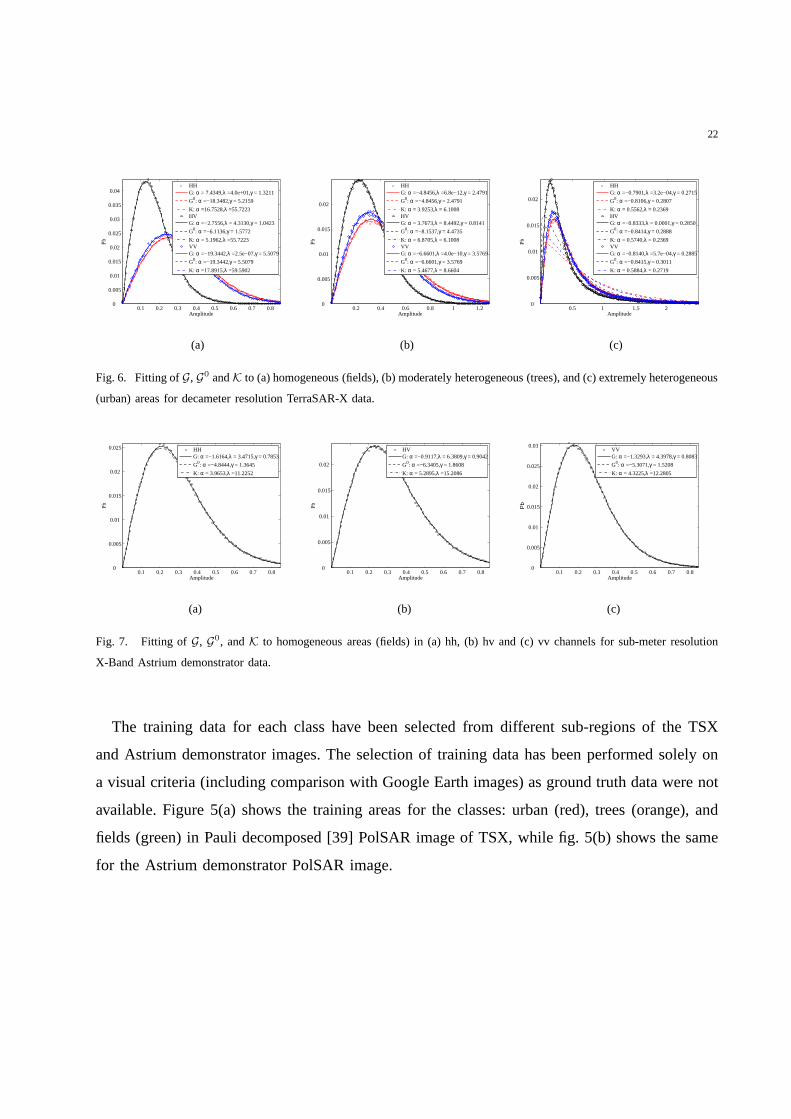
Fig. 6. Fitting ofG, G0 andK to (a) homogeneous (fields), (b) moderately heterogeneous (trees), and (c) extremely heterogeneous
(urban) areas for decameter resolution TerraSAR-X data.
0.1 0.2 0.3 0.4 0.5 0.6 0.7 0.80
0.005
0.01
0.015
0.02
0.025
Amplitude
Pb
HHG: α =−1.6164,λ = 3.4715,γ = 0.7853
G0: α =−4.8444,γ = 1.3645
K: α = 3.9653,λ =11.2252
(a)
0.1 0.2 0.3 0.4 0.5 0.6 0.7 0.80
0.005
0.01
0.015
0.02
Amplitude
Pb
HVG: α =−0.9117,λ = 6.3809,γ = 0.9042
G0: α =−6.3405,γ = 1.8608
K: α = 5.2895,λ =15.2086
(b)
0.1 0.2 0.3 0.4 0.5 0.6 0.7 0.80
0.005
0.01
0.015
0.02
0.025
0.03
Amplitude
Pb
VVG: α =−1.3293,λ = 4.3978,γ = 0.8083
G0: α =−5.3071,γ = 1.5208
K: α = 4.3225,λ =12.2805
(c)
Fig. 7. Fitting ofG, G0, andK to homogeneous areas (fields) in (a) hh, (b) hv and (c) vv channels for sub-meter resolution
X-Band Astrium demonstrator data.
The training data for each class have been selected from different sub-regions of the TSX
and Astrium demonstrator images. The selection of trainingdata has been performed solely on
a visual criteria (including comparison with Google Earth images) as ground truth data were not
available. Figure 5(a) shows the training areas for the classes: urban (red), trees (orange), and
fields (green) in Pauli decomposed [39] PolSAR image of TSX, while fig. 5(b) shows the same
for the Astrium demonstrator PolSAR image.

23
0.2 0.4 0.6 0.8 1 1.2 1.40
0.002
0.004
0.006
0.008
0.01
0.012
0.014
0.016
Amplitude
Pb
HHG: α = 0.5344,λ = 0.7874,γ = 0.0736
G0: α =−1.5903,γ = 0.6985
K: α = 1.1734,λ = 1.2402
(a)
0.2 0.4 0.6 0.8 1 1.2 1.40
0.002
0.004
0.006
0.008
0.01
0.012
0.014
0.016
AmplitudeP
b
HVG: α = 1.1088,λ = 1.5321,γ = 0.0843
G0: α =−2.2769,γ = 1.1576
K: α = 1.6673,λ = 1.9559
(b)
0.2 0.4 0.6 0.8 1 1.2 1.40
0.002
0.004
0.006
0.008
0.01
0.012
0.014
0.016
0.018
0.02
Amplitude
Pb
VVG: α = 0.6366,λ = 0.8469,γ = 0.0554
G0: α =−1.5695,γ = 0.6826
K: α = 1.1708,λ = 1.2428
(c)
Fig. 8. Fitting ofG, G0, andK distributions to moderately heterogeneous areas (trees) in (a) hh, (b) hv and (c) vv channels
for sub-meter resolution X-Band Astrium demonstrator data.
A. Goodness-of-fit to Amplitude Histograms
The marginal intensity distributions ofG, G0p , andKp can be obtained by puttingp = 1 in
(34), (35), and (36), respectively, which reduce to the following intensity distributions:
fZI(zj) =
√λ(
γ +|zj |2σ2j
)(α−1)/2
γα/2πσ2jKα
(
2√λγ) Kα−1
(
2
√
λ
(
γ +|zj |2σ2j
)
)
(44)
fZI(zj) =
2λ(α+1)/2
πσ2jΓ(α)
( |zj|2σ2j
)(α−1)/2
Kα−1
(
2
√
λ|zj|2σ2j
)
(45)
fZI(zj) =
Γ(1− α)(
γ +|zj |2σ2j
)α−1
γαπσ2jΓ(−α)
(46)
wherezj is the j th complex polarimetric channel,j ∈ {hh, hv, vv}, andσ2j is the j th diagonal
element of the ML estimator of normalized covariance matrix, CML , corresponding to thej th
polarimetric channel. The marginal univariate amplitude distributions can be derived by using
the transformationfZA(√zj) = 2fZI
(zj)√zj , resulting in the following closed forms:
fZA(zj) =
2√λ(
γ +|zj|2σ2j
)(α−1)/2
γα/2πσ2jKα
(
2√λγ) Kα−1
(
2
√
λ
(
γ +|zj|2σ2j
)
)
|zj | (47)
fZA(zj) =
4λ(α+1)/2
πσ2jΓ(α)
( |zj |2σ2j
)(α−1)/2
Kα−1
(
2
√
λ|zj |2σ2j
)
|zj | (48)
fZA(zj) =
2Γ(1− α)(
γ +|zj |2σ2j
)α−1
γαπσ2jΓ(−α)
|zj| (49)

24
0.5 1 1.5 2 2.50
0.005
0.01
0.015
0.02
Amplitude
Pb
HHG: α =−0.8655,λ = 0.0000,γ = 0.2090
G0: α =−0.8668,γ = 0.2095
K: α = 0.5601,λ = 0.3591
(a)
0.5 1 1.5 2 2.50
0.002
0.004
0.006
0.008
0.01
0.012
0.014
0.016
0.018
0.02
AmplitudeP
b
HVG: α =−0.6257,λ = 0.0175,γ = 0.1317
G0: α =−0.8079,γ = 0.1745
K: α = 0.6288,λ = 0.5073
(b)
0.5 1 1.5 2 2.50
0.005
0.01
0.015
0.02
0.025
Amplitude
Pb
VVG: α =−0.9469,λ = 0.0000,γ = 0.2437
G0: α =−0.9487,γ = 0.2443
K: α = 0.6487,λ = 0.5090
(c)
Fig. 9. Fitting ofG, G0, andK distributions to extremely heterogeneous areas (urban) in(a) hh, (b) hv and (c) vv channels
for sub-meter resolution X-Band Astrium demonstrator data.
0.2 0.4 0.6 0.8 1 1.20
0.002
0.004
0.006
0.008
0.01
0.012
0.014
0.016
Amplitude
Pb
HHG: α =−2.9121,λ = 0.0000,γ = 1.3689
G0: α =−2.9146,γ = 1.3600
K: α = 2.1827,λ = 3.1132
(a)
0.2 0.4 0.6 0.8 1 1.20
0.005
0.01
0.015
0.02
0.025
0.03
Amplitude
Pb
HVG: α =−2.1488,λ = 0.0000,γ = 0.9079
G0: α =−2.1566,γ = 0.9138
K: α = 1.6342,λ = 2.1965
(b)
0.2 0.4 0.6 0.8 1 1.20
0.002
0.004
0.006
0.008
0.01
0.012
0.014
0.016
Amplitude
Pb
VVG: α =−3.2720,λ = 0.0000,γ = 1.5660
G0: α =−3.2720,γ = 1.5660
K: α = 2.5231,λ = 3.6882
(c)
Fig. 10. Fitting ofG, G0, andK to homogeneous areas (fields) in (a) hh, (b) hv and (c) vv channels for sub-meter resolution
S-Band Astrium demonstrator data.
It must be noted that (48) and (49) are the single-look counterparts of the multi-look marginal
amplitude distributions (KA and G0A) presented in [5], and are thus called the single-lookKA
andG0A distributions, respectively, while (47) is the single-look GA distribution.
Analysis of Results:Figures 6-12 show the fitting ofG, G0, and K distributions to the
histograms of the training classes (urban areas, trees and fields) for each polarimetric channel
of the images considered along with corresponding parameter MLEs listed in the plot legend.
Figure 6 shows this fitting to decameter resolution TSX amplitude histograms for each channel
and each training class. It is evident from the figure that both theG andG0 distributions fit the
data equally good for all classes, while theK distribution fails to fit the data for urban areas.
Figures 7-9 and Figs. 10-12 show theG, G0, andK distribution fittings to the sub-meter

25
TABLE II
MSE AND ρ OF FITTED UNIVARIATE G , G0 , AND K DISTRIBUTIONS FOR SUB-METER RESOLUTIONASTRIUM
DEMONSTRATOR DATA.
Class Pol.pχ2 MSE ρ
G G0 K G G0 K G G0 K
S-band
Urban
hh 0.53 5.9e-5 0.00 7.99e-9 1.48e-8 4.50e-7 0.9991 0.9984 0.9501
hv 0.66 0.00 0.00 9.72e-9 8.36e-8 6.71e-7 0.9992 0.9940 0.9467
vv 0.60 2.0e-3 0.00 8.49e-9 1.44e-8 3.36e-7 0.9991 0.9986 0.9651
Trees
hh 0.39 0.00 0.00 9.41e-9 1.29e-7 1.16e-7 0.9992 0.9906 0.9909
hv 0.30 0.00 0.00 3.95e-8 2.81e-7 3.33e-7 0.9978 0.9861 0.9821
vv 0.11 0.00 0.00 7.66e-9 1.17e-7 1.14e-7 0.9994 0.9921 0.9917
Fields
hh 0.81 0.83 2.4e-3 1.38e-8 1.38e-8 4.55e-8 0.9996 0.9996 0.9988
hv 0.89 0.90 0.00 2.96e-8 2.96e-8 1.83e-7 0.9996 0.9996 0.9976
vv 0.87 0.87 0.00 7.43e-9 7.44e-9 4.77e-8 0.9998 0.9998 0.9987
X-band
Urban
hh 0.61 0.64 0.00 1.08e-8 1.07e-8 9.18e-7 0.9994 0.9994 0.9482
hv 0.69 4.3e-8 0.00 2.41e-8 2.36e-8 8.05e-7 0.9985 0.9984 0.9485
vv 0.69 0.72 0.00 4.19e-9 4.15e-9 7.72e-7 0.9998 0.9998 0.9632
Trees
hh 0.29 0.00 0.00 6.46e-9 2.05e-7 4.53e-8 0.9997 0.9927 0.9983
hv 0.13 0.00 0.00 5.84e-9 1.05e-7 1.51e-8 0.9998 0.9963 0.9994
vv 0.18 0.00 0.00 7.58e-9 2.80e-7 6.77e-8 0.9998 0.9918 0.9979
Fields
hh 0.97 0.11 2.6e-5 7.23e-9 8.63e-9 2.01e-8 0.9999 0.9998 0.9997
hv 0.89 0.05 0.06 5.84e-9 6.80e-9 9.96e-9 0.9999 0.9999 0.9998
vv 0.89 9.5e-5 0.07 8.97e-9 1.46e-8 1.57e-8 0.9999 0.9998 0.9998
resolution X- and S- band Astrium demonstrator data, respectively, for each channel and each
training class. Table II lists the goodness-of-fit measures(χ2, MSE andρ) for these fittings. The
pχ2 values have been used to assess the goodness-of-fit but in some casespχ2 = 0 was obtained
for visually reasonable fittings due to the test’s high dependency on the histogram binning. When
this is the case MSE andρ can be used to further examine the goodness-of-fit. It can be noticed
from the figures and the goodness-of-fit measures in Table II that theG distribution fits the X-
and S-band data very accurately for all the polarimetric channels in all the training classes (high
pχ2 values). TheG0 distribution does not fit trees areas as well as theG distribution (pχ2 = 0,
MSE≈ 1e-7 andρ ≈ 0.990) in both S- and X-band. The same can also be observed for theK

26
0.5 1 1.5 2 2.5 3 0
0.001
0.002
0.003
0.004
0.005
0.006
0.007
0.008
0.009
0.01
Amplitude
Pb
HHG: α =−0.0581,λ = 0.1010,γ = 0.3508
G0: α =−1.2088,γ = 1.3599
K: α = 0.9317,λ = 0.2914
(a)
0.5 1 1.5 2 2.5 3 0
0.002
0.004
0.006
0.008
0.01
0.012
0.014
AmplitudeP
b
HVG: α = 0.1681,λ = 0.1064,γ = 0.1479
G0: α =−0.9880,γ = 0.9527
K: α = 0.8151,λ = 0.2383
(b)
0.5 1 1.5 2 2.5 3 0
0.001
0.002
0.003
0.004
0.005
0.006
0.007
0.008
0.009
0.01
Amplitude
Pb
VVG: α =−0.1074,λ = 0.0986,γ = 0.3865
G0: α =−1.2284,γ = 1.3774
K: α = 0.9434,λ = 0.3009
(c)
Fig. 11. Fitting ofG, G0, andK distributions to moderately heterogeneous areas (trees) in (a) hh, (b) hv and (c) vv channels
for sub-meter resolution S-Band Astrium demonstrator data.
0.5 1 1.5 2 2.5 3 3.5 4 0
0.002
0.004
0.006
0.008
0.01
0.012
Amplitude
Pb
HHG: α =−0.7203,λ = 0.0015,γ = 0.4137
G0: α =−0.8006,γ = 0.4716
K: α = 0.5839,λ = 0.1573
(a)
0.5 1 1.5 2 2.5 3 3.5 4 0
0.002
0.004
0.006
0.008
0.01
0.012
0.014
0.016
0.018
Amplitude
Pb
HVG: α =−0.3954,λ = 0.0113,γ = 0.1889
G0: α =−0.6920,γ = 0.3412
K: α = 0.5402,λ = 0.1404
(b)
0.5 1 1.5 2 2.5 3 3.5 4 0
0.002
0.004
0.006
0.008
0.01
0.012
Amplitude
Pb
VVG: α =−0.8085,λ = 0.0015,γ = 0.5049
G0: α =−0.8775,γ = 0.5589
K: α = 0.6406,λ = 0.1940
(c)
Fig. 12. Fitting ofG, G0, andK distributions to extremely heterogeneous areas (urban) in(a) hh, (b) hv and (c) vv channels
for sub-meter resolution S-Band Astrium demonstrator data.
distribution. However, theG0 distribution fits the fields areas much better (better in S-band than
in X-band) and also fits urban areas reasonably well (better in X-band than in S-band) but still
not better than theG distribution (lowerpχ2 values). Note that there are some cases whereG0
shows slightly higherpχ2 values than theG distribution e.g. S-band fields hh, hv and X-band
urban hh, vv but the∆pχ2 is very small and can be ignored, so these cases can be treatedas
equally good fittings. In addition to this, theK distribution, as expected, fails to model urban
areas and performs reasonably well for fields (better in X-band than in S-band), although the
pχ2 values are very close to zero.
A direct comparison of the heterogeneity of the observed scene can also be made between
the X- and S-bands data to see the effect of frequency change when all other radar parameters
are the same. For this purpose, the PDFs fitting to amplitude histograms of homogeneous areas

27
TABLE III
MULTIVARIATE & AVERAGED UNIVARIATE MLES OFG DISTRIBUTION PARAMETERS FOR SUB-METER RESOLUTION
ASTRIUM DEMONSTRATOR DATA.
Classα, λ, γ
Multivariate MLE Averaging MLE
Astrium demonstrator S-band
Urban -0.5955, 0.0040, 0.3221 -0.6414, 0.0048, 0.3692
Trees 0.0312, 0.1035, 0.2696 8.95e-4 0.1020, 0.2951
Fields -2.4995, 3.92e-14, 1.1226 -2.7777, 9.58e-13, 1.2809
Astrium demonstrator X-band
Urban -0.8725, 8.59e-5, 0.2148 -0.8127, 0.0058, 0.1948
Trees 0.7506, 1.0967, 0.0924 0.7599, 1.0555, 0.0711
Fields -2.6967, 3.6935, 1.1520 -1.2858, 4.7501, 0.8326
TSX X-band
Urban -0.8120, 3.14e-4, 0.2870 -0.8125, 3.27e-4, 0.2817
Trees -6.2319, 4.02e-12, 3.3217 -2.5794, 2.8164, 2.2900
Fields -7.1559, 2.6592, 2.1587 -4.8883, 14.8534, 2.6238
between X- and S-bands can be compared between Fig. 7 and Fig.10, respectively. It can be
readily distinguished that the amplitude histogram of S-band data shown in Fig. 10 shows a
deviation from the K-distribution fitting (representing the Rayleigh distributed amplitude case),
while, in contrast to this, the amplitude histogram of X-band data in Fig. 7 shows nearly full
agreement with the K-distribution fitting. This shows that the observed scene is slightly more
heterogeneous in S-band than in X-band at the above mentioned radar parameters.
B. Naıve MAP Classification of S-band PolSAR Image
The MLEs of the more accurateG distribution have been numerically computed over fields,
trees, and urban areas by using the multivariate MLE method and the averaging MLE method
described in section V. These parameter estimates have beenlisted in Table III. A comparison of
the corresponding MLEs from multivariate MLE method and averaging MLE method in Table
III shows that both provide very close parameter estimates for lower values of the parameters
as observed earlier for simulated PolSAR data, but deviate considerably from each other for
higher parameter values. The MLEs obtained from the averaging MLE method have been used

28
Az
Rg
(a) (b)
Fig. 13. (a) Portion of the pauli color coded Astrium demonstrator Baginton S-band image (750× 1000 pixels) used as an
independent test data for MAP classificationc© EADS Astrium Ltd., and (b) the corresponding optical imagec© 2011 Infoterra
Ltd.
for classification as it has been noticed in section V that they are more accurate than the ones
obtained using multivariate MLE method.
A simple MAP classifier can be used to classify an independenttest data (750× 1000
pixels) extracted from Astrium demonstrator Baginton S-band image shown in Fig. 13 alongside
its optical counterpart. The MAP classifier can be conveniently represented by the following
expression:
z → ωi if
P (ωi|z) =m
maxj=1
P (z|ωj)P (ωj) (50)
whereωj represents thej th class, and the input vector z is assigned the classωi with the maximum
aposteriori probability.
Analysis of Results:Figure 14 shows the image after applying the MAP classifier using the
G distribution with MLEs from averaging MLE method listed in Table III for each class. Also,
the color codes of different classes have been listed in the figure.
A visual comparison of Fig. 14 and its optical counterpart inFig. 13 shows that the clas-
sification identifies urban areas, trees, and fields considerably well. Some of the errors could
be attributed to inaccurate training data, as manual procedures have been used for selection of
training data. Further, the temporal difference between the acquisition of radar and optical images
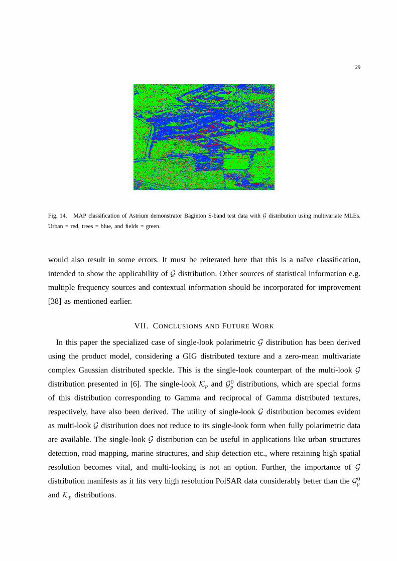
29
Fig. 14. MAP classification of Astrium demonstrator Baginton S-band test data withG distribution using multivariate MLEs.
Urban = red, trees = blue, and fields = green.
would also result in some errors. It must be reiterated here that this is a naıve classification,
intended to show the applicability ofG distribution. Other sources of statistical information e.g.
multiple frequency sources and contextual information should be incorporated for improvement
[38] as mentioned earlier.
VII. CONCLUSIONS AND FUTURE WORK
In this paper the specialized case of single-look polarimetric G distribution has been derived
using the product model, considering a GIG distributed texture and a zero-mean multivariate
complex Gaussian distributed speckle. This is the single-look counterpart of the multi-lookGdistribution presented in [6]. The single-lookKp andG0p distributions, which are special forms
of this distribution corresponding to Gamma and reciprocalof Gamma distributed textures,
respectively, have also been derived. The utility of single-look G distribution becomes evident
as multi-lookG distribution does not reduce to its single-look form when fully polarimetric data
are available. The single-lookG distribution can be useful in applications like urban structures
detection, road mapping, marine structures, and ship detection etc., where retaining high spatial
resolution becomes vital, and multi-looking is not an option. Further, the importance ofGdistribution manifests as it fits very high resolution PolSAR data considerably better than theG0pandKp distributions.

30
The proposedG distribution has been found to fit sub-meter resolution X- & S-band Astrium
demonstrator PolSAR data better than, and decameter resolution X-band TerraSAR-X PolSAR
data as good as theG0p distribution. Under the given radar parameters it has also been observed
that the scene shows more heterogeneity in S-band compared to X-band. Although the proposed
distribution is computationally expensive as it has three parameters, it out performs the fitting
accuracy ofG0p & Kp distributions. The fitting of these distributions to PolSARdata has been
presented by using univariate fitting to amplitude histograms. TheG distribution fits the ampli-
tude histograms of homogeneous, moderately heterogeneous, and extremely heterogeneous areas
accurately even where theG0p andKp perform relatively poorly. The application ofG distribution
to statistically model PolSAR data has also been shown by using a naıve MAP classifier on an S-
band PolSAR image. A qualitative visual evaluation of the classification shows thatG distribution
can be used as an effective underlying statistical model as all the three classes of urban, trees,
and fields areas are reasonably identified.
Maximum Likelihood Estimation (MLE), using Matlab’s Simplex algorithm, has been used for
parameter estimation. The convergence of the Simplex algorithm to globally maximum likelihood
function values has been shown by using simulated PolSAR data and comparing the results
with a global maximization algorithm based on Simulated Annealing and Simplex algorithms
(SIMPSA). It has been found that the Simplex algorithm always converges to globally maximum
values of likelihood function for data of the order of 0.1 million points. It has also been shown
that the parameter estimates of the multivariateG distribution can be computed more accurately
by using the average of single-channel estimates instead ofcomputing estimates from multivariate
PolSAR data. This has been shown on simulated PolSAR data fora variety of backscattering
textures. Also, a new algorithm for accurate estimation of speckle covariance matrix has been
proposed.
One of the drawbacks of the current analysis is that the texture has been modeled as the
square root of a positive random variable instead of more accurately modeling it as the square
root of a diagonal matrix variate with the texture of each polarimetric channel separated along
the diagonal. Such a technique has been very recently adopted in [40], and is one of the areas
of future work. Also, the GIG texture in simulated PolSAR data was generated withα > 0 only,
due to limitation of the used GIG random number generator. A GIG random number generator
with α ∈ R would be desirable. Another area of improvement is the selection of accurate training

31
data for fitting analysis instead of a visual selection approach. Nevertheless, the superior fitting
accuracy of the proposed single-lookG distribution, especially in the case of sub-meter resolution
PolSAR data, will be significant in improving classification, segmentation, and feature extraction
algorithms for VHR single-look PolSAR data in various applications including but not limited
to urban structures detection, road mapping, marine structures and ship detection.
ACKNOWLEDGMENT
The authors would like to kindly thank DLR (German AerospaceCenter) and EADS Astrium
Ltd. for providing the datasets.
REFERENCES
[1] J.-S. Lee and E. Pottier,Polarimetric Radar Imaging: From Basics to Applications. Boca Raton, FL: CRC Press, Taylor
& Francis Group, 2009, ch. 4, pp. 101–107.
[2] C. Oliver and S. Quegan,Understanding Synthetic Aperture Radar Images, 2nd ed. Raleigh, NC: SciTech Publishing,
2004, ch. 5, pp. 130–135.
[3] A. Doulgeris and T. Eltoft, “Scale mixture of Gaussians modelling of polarimetric SAR data,”EURASIP J. Adv. Signal
Process, vol. 2010, no. 874592, pp. 1–12, Jan. 2010.
[4] L. Bombrun and J.-M. Beaulieu, “Fisher distribution fortexture modeling of polarimetric SAR data,”IEEE Geosci. Remote
Sens. Lett., vol. 5, no. 3, pp. 512–516, Jul. 2008.
[5] A. Frery, H.-J. Muller, C. Yanasse, and S. Sant’Anna, “A model for extremely heterogeneous clutter,”IEEE Trans. Geosci.
Remote Sens., vol. 35, no. 3, pp. 648–659, May 1997.
[6] C. Freitas, A. Frery, and A. Correia, “The polarimetricG distribution for SAR data analysis,”Environmetrics, vol. 16,
no. 1, pp. 13–31, Feb. 2005.
[7] G. Gao, “Statistical modeling of SAR images: A survey,”Sensors, vol. 10, no. 1, pp. 775–795, Jan. 2010.
[8] V. Amberg, M. Coulon, P. Marthon, and M. Spigai, “Structure extraction from high resolution SAR data on urban areas,”
in Proc. IGARSS, Anchorage, AK, 2004, vol. 3, Sep. 2004, pp. 1784–1787.
[9] ——, “Improvement of road extraction in high resolution SAR data by a context-based approach,” inProc. IGARSS, Seoul,
Korea, 2005, vol. 1, Jul. 2005, pp. 490–493.
[10] M. Migliaccio, A. Gambardella, and F. Nunziata, “Ship detection over single-look complex SAR images,” inIEEE/OES
US/EU-Baltic International Symposium, 2008, May 2008, pp. 1–4.
[11] L. Bombrun, G. Vasile, M. Gay, and F. Totir, “Hierarchical segmentation of polarimetric SAR images using heterogeneous
clutter models,”IEEE Trans. Geosci. Remote Sens., vol. 49, no. 2, pp. 726–737, Feb. 2011.
[12] J. W. Goodman, “Some fundamental properties of speckle,” J. Opt. Soc. Am., vol. 66, no. 11, pp. 1145–1150, Nov. 1976.
[13] C. Oliver and S. Quegan,Understanding Synthetic Aperture Radar Images, 2nd ed. Raleigh, NC: SciTech Publishing,
2004, ch. 11, pp. 326–327.
[14] N. R. Goodman, “Statistical analysis based on a certainmultivariate complex Gaussian distribution (an introduction),” Ann.
Math. Stat., vol. 34, no. 1, pp. 152–177, Mar. 1963.

32
[15] F. Gini and M. Greco, “Covariance matrix estimation forCFAR detection in correlated heavy tailed clutter,”Signal Process.,
vol. 82, no. 12, pp. 1847–1859, Dec. 2002.
[16] F. Pascal, Y. Chitour, J.-P. Ovarlez, P. Forster, and P.Larzabal, “Covariance structure maximum-likelihood estimates in
compound Gaussian noise: Existence and algorithm analysis,” IEEE Trans. Signal Process., vol. 56, no. 1, pp. 34–48, Jan.
2008.
[17] G. Vasile, J.-P. Ovarlez, F. Pascal, and C. Tison, “Coherency matrix estimation of heterogeneous clutter in high-resolution
polarimetric SAR images,”IEEE Trans. Geosci. Remote Sens., vol. 48, no. 4, pp. 1809–1826, Apr. 2010.
[18] Y. Chitour and F. Pascal, “Exact maximum likelihood estimates for SIRV covariance matrix: Existence and algorithm
analysis,”IEEE Trans. Signal Process., vol. 56, no. 10, pp. 4563–4573, Oct. 2008.
[19] R. Muirhead,Aspects of multivariate statistical theory. Hohoken, NJ: John Wiley and Sons, Inc., 1982, ch. 2, pp. 61–62.
[20] J.-S. Lee and E. Pottier,Polarimetric Radar Imaging: From Basics to Applications. Boca Raton, FL: CRC Press, Taylor
& Francis Group, 2009, ch. 3, pp. 113–114.
[21] S. Anfinsen, T. Eltoft, and A. Doulgeris, “A relaxed Wishart model for polarimetric SAR data,” inProc. PolInSAR, Frascati,
Italy, 2009.
[22] H. H. Lim, A. A. Swartz, H. A. Yueh, J. A. Kong, R. T. Shin, and J. J. van Zyl, “Classification of earth terrain using
polarimetric Synthetic Aperture Radar images,”J. Geophys. Res., vol. 94, no. B6, pp. 7049–7057, 1989.
[23] S. Quegan, I. Rhodes, and R. Caves, “Statistical modelsfor polarimetric SAR data,” inProc. IGARSS, Pasadena, CA,
1994, vol. 3, Aug. 1994, pp. 1371–1373.
[24] J. Lee, D. Schuler, R. Lang, and K. Ranson, “K-distribution for multi-look processed polarimetric SAR imagery,” inProc.
IGARSS, Pasadena, CA, 1994, vol. 4, Aug. 1994, pp. 2179–2181.
[25] J.-M. Beaulieu and R. Touzi, “Segmentation of texturedpolarimetric SAR scenes by likelihood approximation,”IEEE
Trans. Geosci. Remote Sens., vol. 42, no. 10, pp. 2063–2072, Oct. 2004.
[26] S. H. Yueh, J. A. Kong, J. K. Jao, R. T. Shin, and L. M. Novak, “K-distribution and polarimetric terrain radar clutter,” J.
Electrom. Waves Appl., vol. 3, pp. 747–768, Aug. 1989.
[27] C. Tison, J.-M. Nicolas, F. Tupin, and H. Maitre, “A new statistical model for Markovian classification of urban areas in
high-resolution SAR images,”IEEE Trans. Geosci. Remote Sens., vol. 42, no. 10, pp. 2046–2057, Oct. 2004.
[28] C.-W. Chou and W.-J. Huang, “On characterizations of the Gamma and Generalized Inverse Gaussian distributions,”Stat.
Probab. Lett., vol. 69, no. 4, pp. 381–388, 2004.
[29] L. Andrews and R. Phillips,Mathematical Techniques for Engineers and Scientists. New Delhi-110001: Prentice-Hall of
India, 2005, ch. 13, p. 677.
[30] D. Cross, “On the relation between real and complex Jacobian determinants.” May 2008, unpublished. [Online]. Available:
http://www.brynmawr.edu/physics/DJCross/docs/papers/jacobian.pdf
[31] R. Tough, D. Blacknell, and S. Quegan, “Estimators and distributions in single and multi-look polarimetric and
interferometric data,” inProc. IGARSS, Pasadena, CA, 1994, vol. 4, Aug. 1994, pp. 2176–2178.
[32] J. Lagarias, J. Reeds, M. Wright, and P. Wright, “Convergence properties of the Nelder-Mead Simplex method in low
dimensions,”SIAM Journal of Optimization, vol. 9, pp. 112–147, 1998.
[33] A. Frery, F. Cribari-Neto, and M. Souza, “Analysis of minute features in speckled imagery with maximum likelihood
estimation,”EURASIP J. Appl. Signal Process., vol. 2004, no. 16, pp. 2476–2491, Jan. 2004.
[34] M. Rangaswamy, D. Weiner, and A. Ozturk, “Computer generation of correlated non-Gaussian radar clutter,”IEEE Trans.
Aerosp. Electron. Syst., vol. 31, no. 1, pp. 106–116, Jan. 1995.

33
[35] J.-S. Lee and E. Pottier,Polarimetric Radar Imaging: From Basics to Applications. Boca Raton, FL: CRC Press, Taylor
& Francis Group, 2009, ch. 4, pp. 114–115.
[36] J. Dagpunar, “An easily implemented generalized inverse Gaussian generator,”Commun. Statist. -Simula., vol. 18, no. 2,
pp. 703–710, 1989.
[37] M. Cardoso, R. Salcedo, and S. Feyo de Azevedo, “The simplex-simulated annealing approach to continuous non-linear
optimization,” Computers Chem. Eng., vol. 20, no. 9, pp. 1065–1080, 1996.
[38] A. Frery, A. Correia, and C. da Freitas, “Classifying multifrequency fully polarimetric imagery with multiple sources of
statistical evidence and contextual information,”IEEE Trans. Geosci. Remote Sens., vol. 45, no. 10, pp. 3098–3109, Oct.
2007.
[39] J.-S. Lee and E. Pottier,Polarimetric Radar Imaging: From Basics to Applications. Boca Raton, FL: CRC Press, Taylor
& Francis Group, 2009, ch. 4, pp. 63–65.
[40] T. Eltoft, S. Anfinsen, and A. Doulgeris, “A multitexture model for multilook polarimetric radar data,” inProc. IGARSS,
Vancouver, BC, 2011, Jul. 2011, pp. 1048–1051.
Salman Khan was born in Lahore, Pakistan in 1982. He received B.S. degreein Computer Sciences from
National University of Computer and Emerging Sciences, Pakistan in 2004, the M.S. degree in Electrical
Engineering as a Fulbright scholar from University of Central Florida, Orlando, U.S.A. in 2009, and is
currently in the second year of Ph.D. in Electronics Engineering (Remote Sensing) at the Surrey Space
Centre, University of Surrey in Guildford, U.K.
His research interests include statistical and physical model based analysis of polarimetric SAR images,
and pattern recognition.
Related Documents